Embed Size (px)
Citation preview

Financial Intermediation, International Risk Sharing,
and Reserve Currencies
Matteo Maggiori∗
Job Market Paper
November 2011
Abstract
I provide a framework for understanding the global financial architecture as an
equilibrium outcome of the risk sharing between countries with different levels of
financial development. The country that has the most developed financial sector
takes on a larger proportion of global fundamental and financial risk because its
financial intermediaries are better able to deal with funding problems following
negative shocks. This asymmetric risk sharing has real consequences. In good times,
and in the long run, the more financially developed country consumes more, relative
to other countries, and runs a trade deficit financed by the higher financial income
that it earns as compensation for taking greater risk. During global crises, it suffers
heavier capital losses than other countries, exacerbating its fall in consumption. This
country’s currency emerges as the world’s reserve currency because it appreciates
during crises and so provides a good hedge. The model is able to rationalize these
facts, which characterize the role of the US as the key country in the global financial
architecture.
JEL classification: E44, F31, F32, F33, G01, G15, G21.
Keywords: Global Liquidity, International Portfolios, Exorbitant Privilege,Global Imbalances, Global Saving Glut.
∗Haas School of Business, Finance Department, University of California, Berkeley.matteo [email protected]. Tel: +1 510 501 4497. Website: faculty.haas.berkeley.edu/Maggiori.I would like to thank the members of my PhD committee for advice well beyond their duties: NicolaeGarleanu, Pierre-Olivier Gourinchas, Martin Lettau, Maurice Obstfeld, and Andrew Rose. I would alsolike to thank: Mark Gertler, Nobuhiro Kiyotaki, Hanno Lustig, Helene Rey, Johan Walden, and seminarparticipants at UC Berkeley (international macroeconomics, macro lunch, finance) and the LondonBusiness School (economics). I gratefully acknowledge the financial support of the White Foundationand the UC Berkeley Institute for Business and Economics Research.
The global financial architecture is characterized by the existence of a key country.
This role has been fulfilled by the United States of America (US) since the Second World
War; prior to the First World War it was fulfilled by the United Kingdom (UK). An
important characteristic of the key country is the depth of its financial markets and, in
particular, of its funding markets. The empirical literature has highlighted stylized facts
that characterize the US international position: its external portfolio is characterized
by riskier assets than liabilities; it runs a persistent trade deficit; it transfers wealth to
the rest of the world (RoW) during global crises; and its currency is the world’s reserve
currency and earns a safety premium.
Despite extensive debates on the factors underpinning the global financial architecture,
as well as its sustainability, there are few formal models that analyze its economic
foundations. I provide a theoretical framework based on financial frictions that
rationalizes the role of the key country in the global financial architecture and jointly
explains the stylized facts that characterize the US external position.
The key country has the most developed financial sector and takes on a larger
proportion of global fundamental and financial risk because its financial intermediaries
are better able to deal with funding problems following negative shocks. In good times
and in the long run it consumes more, relative to other countries, and runs a trade deficit
financed by the higher financial income that it earns as compensation for taking greater
risk. During global crises, however, capital losses on its external portfolio lead to a wealth
transfer to the RoW. This increases the wealth loss suffered by the key country as a result
of the crisis and exacerbates the fall in its consumption.
The key country’s currency emerges as the reserve currency because it appreciates
during crises, thus representing a global safe asset. This occurs, despite the key country’s
wealth losses, because of shifts in the relative demand for goods. The increase in the
RoW’s relative demand for RoW goods, which originates from the wealth transfer from
the key country to the RoW, is more than offset by the fall in the key country’s relative
demand for RoW goods, which originates from increased RoW export costs.
The model not only provides a theoretical framework that jointly makes sense of the
empirical stylized facts; its main contribution is to do so by providing the underlying
1
economic foundations through the explicit modeling of financial intermediation and its
frictions. The model recognizes the importance of financial intermediation from the key
country as both the means of sharing risks globally and a potential source of risk and
instability for the global financial architecture.
The model shows that the global financial architecture is affected by endogenous
financial instability, with negative fundamental shocks being amplified by the financial
system. The amplification occurs because financial intermediaries are levered and invest
in similar risky assets; the resulting systemic risk exacerbates the effects of adverse shocks
through a fire-sale mechanism.
I summarize the empirical evidence that motivates this paper in four stylized facts:
Fact 1: The US external balance sheet is characterized by risky assets, mainly
denominated in foreign currencies, and safer liabilities, mainly denominated in US dollars.
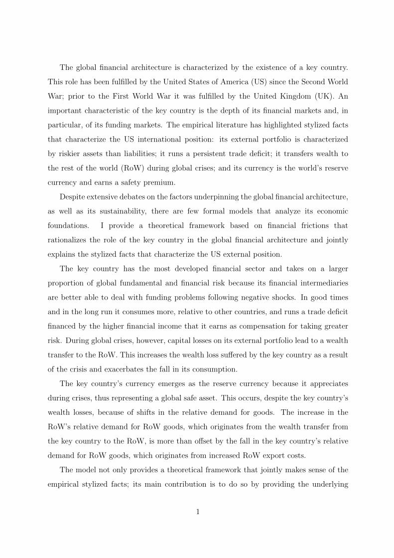
Figure 1 shows the US external balance sheet, as of year-end 2007. US residents’ holdings
of foreign assets were focused on riskier assets, such as equity and foreign direct investment
(FDI), which together accounted for 56% of total US assets. By contrast, foreign residents’
holdings of US assets were concentrated in safer assets such as debt, which accounted for
69% of total US liabilities.1 Figure 2 confirms this by plotting the above percentages for
1970-2010. Figure 3 highlights that the majority of US external assets, 64% on average,
are denominated in foreign currencies. US external liabilities are instead predominantly
denominated in US dollars, 90% on average.2
Fact 2: The US runs a persistent trade deficit. The US has run a trade deficit every
year since 1976; in 2010, its trade deficit was 3.4% of GDP.3
Fact 3: During global crises, the US transfers substantial amounts of wealth to the
RoW. The US net foreign asset position deteriorated by $1.4 trillion in 2008. This
corresponds to a transfer of 10% of US GDP to the RoW over that year.4
Fact 4: The US dollar is the world reserve currency and earns a safety premium.
1Source: Balance of Payment Statistics. The percentages are computed as (Equity+FDI)/(Total Assets-Derivatives) and (Debt+Other Investments)/(Total Liabilities-Derivatives).2Source: Lane and Shambaugh (2010). The average is for the period 1990-2004.3Source: IMF.4Source: Balance of Payment Statistics and author’s calculations. The deterioration is due in part tochanges in the US external portfolio positions and in part to capital losses. I calculate that the capitallosses alone constitute a transfer of 7.5% of US GDP. See also Gourinchas, Rey, and Truempler (2011).
2

Institutions around the world, both private and governmental, hold reserves of US dollars.5
Figure 4 shows the estimated6 compensation required by investors for holding a basket of
foreign currencies while funding themselves in US dollars: the US dollar safety premium.
The annualized premium is, on average, 1%; however, it increases significantly in times
of crisis. At the height of the recent financial crisis in October 2008, the US dollar safety
premium was as high as 53%.
To make sense of these facts I introduce three successive models. In Section II, I
introduce a general-equilibrium model of financial intermediation in a closed economy.
This autarky model highlights the mechanisms that play an important role in the open
economy case; however, its implications for asset pricing are of independent interest. In
Section III, I introduce a simple open economy model with two countries and a single
world endowment. This model highlights the core result of the paper: the asymmetric
risk sharing between the key country and the RoW, from which Facts 1-3 emerge. This
model cannot account for Fact 4 because, by design, no exchange rate is present. In
Section IV, I allow each country to have an endowment of a differentiated good. In
addition to considering how financial frictions affect demand for financial assets, I also
consider how they affect demand for goods by introducing trade costs. This final model
not only allows me to analyze the exchange rate, but also generalizes the results from the
previous section.
In the autarky model in Section II, savings are deposited with financial intermediaries,
which in turn invest in risky assets. Since financial intermediaries may choose not to
repay their depositors, their funding is potentially credit constrained. When financial
intermediaries are well capitalized, the high level of capital acts as a safety buffer against
potential investment losses; they can therefore easily raise funding and invest in risky
assets. When financial intermediaries are poorly capitalized, concerns over their viability
restrict their funding and therefore curtail their ability to invest in risky assets. Financial
intermediaries are concerned about two sources of risk: fundamental risk and financial5Eichengreen (2011, page 64) shows that 63% of world official reserves were held in US dollars at year-end2009, a figure close to the average for the period 1965-2009.6See Maggiori (2010) for details of the estimation. Lustig, Roussanov, and Verdhelan (2010) provideevidence of a counter-cyclical US dollar currency premium.
3
risk. The former stems from variations in output, while the latter results from variations in
the aggregate capital of financial intermediaries. In equilibrium, the presence of financing
frictions induces intermediaries to discount risky assets more than in a frictionless model.
In the open economy model in Section III, the greater depth of the US’s financial
development is represented by the key country’s financial intermediaries being better able
to raise funding for investment purposes, even when they are poorly capitalized. This, in
turn, induces the key country’s financial intermediaries to be less concerned about taking
leveraged risk: in equilibrium, they take more risk. On the other hand, RoW financial
intermediaries accumulate precautionary long positions in safer assets in order to insulate
their capital from negative shocks. The asymmetric US balance sheet (Fact 1 ) emerges
from this asymmetric risk sharing. The US trade deficit (Fact 2 ) emerges from the higher
consumption that it enjoys in good times and in the long run, as compensation for the
greater risks that it takes. Similarly, wealth transfers occur in bad times (Fact 3 ) because
of the heavier losses suffered by the key country following negative shocks.
The role of the US dollar as a global safe asset is challenging to explain within
traditional models. These would predict that a transfer of wealth from the US to the
RoW during crises would result in a US dollar depreciation, because the wealth transfer
would increase the relative demand for RoW goods, as long as the RoW residents were
spending a higher proportion of the wealth that they received on RoW goods than on
US goods. If this were the case, the US dollar would represent a risky asset for RoW
residents, since it would pay low in bad states of the world.
The tension between the wealth transfer from the US to the RoW and the role of
the US dollar as a global safe asset creates a “reserve currency paradox”. In Section IV,
I rationalize these seemingly contradictory forces by showing that the paradox can be
resolved if, in addition to the channel described above, the US relative demand for US
goods also increases during crises. I directly model a set-up where RoW export costs
increase whenever RoW financial intermediaries lose capital and decrease the availability
of credit to RoW exporters. A less literal interpretation of the model also accommodates
frameworks where US and RoW exports are differentiated and, in particular, where the
demand for US goods is more resilient to global downturns.
4

I Related Literature
The closed economy model contributes to the study of the implications of the financial
sector for macroeconomics and finance, in the tradition7 of Bernanke and Gertler (1989)
and Kiyotaki and Moore (1997). In particular, it adapts the modeling of financial
intermediation of Gertler and Kiyotaki (2010)8 to a continuous-time endowment-economy
framework. These modifications allow me to provide global solutions,9 analyze risk
premia, and characterize both the stochastic steady state and the stationary distribution
of wealth. The global solutions, which are analytical up to the solution of a system
of two ordinary differential equations (ODEs), show that the equilibrium has substantial
non-linearities that cannot be readily analyzed by log-linearizing around the deterministic
steady state. This solution method also allows me to exactly characterize the international
portfolios in the open economy model.
The key assumption of greater financial development10 of the US compared to the
RoW is in the spirit of Caballero, Farhi, and Gourinchas (2008) and Mendoza, Quadrini,
and Rıos Rull (2009). Kindleberger (1965) and Despres, Kindleberger, and Salant (1966)
were among the first to argue that the asymmetric external balance sheet of the US, and
previously of the UK, could be due to differences in financial development. Caballero
et al. (2008) analyze a deterministic model where the US’s greater ability to supply
tradable assets rationalizes the emergence of global imbalances, the US trade deficit,
and low long-term interest rates. Mendoza et al. (2009) analyze a production economy
with idiosyncratic risk and limited contract enforceability, where the US’s greater ability
to enforce contracts leads to a lower US interest rate and an asymmetric US balance
7For a sample of this literature see: Bernanke, Gertler, and Gilchrist (1999), Fostel and Geanakoplos(2008), Simsek (2009), Kurlat (2009), He and Krishnamurthy (2010), Brunnermeier and Sannikov (2010),Garleanu and Pedersen (2011).8This paper builds on the work of Gertler and Karadi (2011) and Kiyotaki and Moore (2008).9“Global” refers to solving the equations that characterize the equilibrium of the model for the entirerange of the state variables, rather than solving them by a log-linear approximation of the model aroundthe non-stochastic steady state.10I am not suggesting that financial development is the only characteristic. Recent literature, for example,has emphasized the importance of country size for currency returns (Hassan (2010), Martin (2011)). Mygoal is to isolate the role of one important characteristic, financial development, and to analyze itsequilibrium implications.
5

sheet. The most closely related work is that of Gourinchas, Govillot, and Rey (2010),11
who study the role of the US as an insurance provider to the RoW in a representative
agent framework with complete markets, where agents differ in the coefficient of relative
risk aversion.
I add to this literature not only by providing a risk-based view of the role of the key
country, which differs from the traditional macroeconomic view; more importantly, I do
so by providing the underlying economic foundations through the explicit modeling of
financial sector frictions and aggregate risk. The former is important to understanding
the characteristics that distinguish the key country and its role, while the latter allows
me to analyze the benefits and the costs of asymmetric risk sharing, especially during
financial crises.
I also analyze exchange rate dynamics, which are important to understanding why
the RoW considers US-dollar-denominated short-term debt to be safe. Previous papers
do not model the role of the US dollar as a reserve currency or its safety premium. In
addition, the risk-based view of the key currency that I provide is in contrast to Krugman
(1980) and Matsuyama, Kiyotaki, and Matsui (1993), who instead stress the vehicle role
of the key currency for international trade.
II Autarky: the Banking Economy
The output of the economy is determined by a tree with stochastic dividend process
dY (t)
Y (t)= µ dt+ σ dz(t), (1)
where z(t) is a standard Brownian motion,12 and µ and σ are constant.
The set-up of financial intermediation is a continuous time adaptation of Gertler and
Kiyotaki (2010). The economy is populated by a continuum of measure one of households.
11The paper also provides evidence that the US earns positive excess returns on its external portfolio.See Curcuru, Dvorak, and Warnock (2008) for a contrarian view.12The Brownian motion is defined on a complete probability space and generates a filtration F .Throughout the paper, “adapted process” means F (t) adapted. For brevity, I state all results withoutexplicitly referencing the regularity conditions necessary for the applications of stochastic calculus in thispaper. Where necessary, some regularity conditions are explicitly verified in the proofs in Appendix A.
6
Each household consists of a continuum of measure one of family members, or agents, of
which a fraction β ∈ (0, 1) are savers and a fraction 1 − β are financiers. All agents,
both savers and financiers, have logarithmic utility and identical rate of time preferences.
Each financier within a household manages a financial intermediary; these are all, in turn,
owned by the household. Savers deposit funds with these financial intermediaries.
By assumption, there is perfect consumption insurance within each household because
all agents pay out their earnings to be shared equally across the entire household. This
assumption, combined with an application of the law of large numbers across households,
allows for the construction of the representative agent.
In order to create a meaningful role for financial intermediation, I assume that
only financiers, through their financial intermediaries, can hold shares in the output
tree.13 Savers can only deposit funds with financial intermediaries and they receive a
pre-determined return rd(t).
The saver’s problem, therefore, is to choose how much to consume and how much to
deposit with the financial intermediaries:
maxC(u)∞u=t
Et
[∫ ∞
t
e−ρ(u−t)log(C(u))du
](2)
s.t. dD(t) = [rd(t)D(t)− C(t)]dt+ Π(t)dt,
where D is the aggregate savers’ deposits and Π is the aggregate net transfers from the
financiers, described later. Because the economy has a representative agent, I directly
write the saver’s optimization problem in terms of aggregate quantities. Throughout
the paper, upper-case letters denote aggregate quantities, while lower-case letters denote
individual agents’ quantities. In addition, I use the equilibrium outcome of no default on
deposits to directly write the dynamics of the deposit account as being risk free.
Financiers can use their own capital and the deposits that they have raised to invest
in the risky asset. The balance sheet of a financial intermediary is Q(t)s(t) = n(t) + d(t),
where s(t) is the number of shares of the output tree owned by the financial intermediary,
13A number of papers motivate this assumption by developing micro-foundations where monitoringproblems make it inefficient for savers to directly hold assets. These papers delegate the asset managementproblem to financial intermediaries in equilibrium. I follow Gertler and Kiyotaki (2010) in directlyassuming that an unmodelled monitoring problem prevents savers from directly holding assets.
7
Q(t) is the price of the output tree, and n(t) is the financial intermediary’s net worth.
The stock price dynamics follow the continuous diffusion process
dQ(t)
Q(t)+
Y (t)
Q(t)dt = µQ(t)dt+ σQ(t)dZ(t).
The drift and volatility terms need to be solved for in equilibrium.
Financiers face a credit constraint, which requires that the value of the financial
intermediary that they manage remains positive. To motivate this constraint, I introduce
an incentive compatibility problem. Financiers can walk away from their financial
intermediary; if this occurs, the financial intermediary is wound down and its depositors
recover the value of the financial intermediary’s assets: s(t)Q(t).14
Savers only deposit funds with financial intermediaries owned by other households.
In particular, they spread their deposits sufficiently across the financial intermediaries
owned by the various households to allow the law of large numbers to hold.15 This allows
a simple aggregation of the model, while still maintaining a meaningful incentive for
financiers to walk away from negative net worth financial intermediaries. In short, the
incentive compatibility problem provides the micro foundations for a credit constraint.
Since financiers and savers have identical utility functions, there are no incentives for
financiers to pay dividends from their financial intermediaries. Instead, financiers would
choose to accumulate capital and their financial intermediaries would “grow out” of the
credit constraint. To prevent this outcome, I assume that financiers and savers switch
roles based on exponential probability functions with intensity λ and λ1−ββ , respectively.16
When a financier switches role, she pays all her accumulated net worth to her household.
14More precisely, savers receive min(s(t)Q(t), d(t), with excess funds, if any, being returned to thefinancier’s household. In equilibrium, however, the financier has no incentive to walk away from thefinancial intermediary if its deposits can be fully recovered, so the simplified formulation is adopted inthe main text.15To motivate this assumption one can think of a set-up with idiosyncratic risk in each intermediary, suchthat savers want to diversify their deposits across intermediaries, and then let this risk shrink to zero.16The different intensities maintain the populations of savers and financiers constant.
8

The financier’s optimization problem is, therefore, to maximize the value of the
financial intermediary that she manages, subject to the credit constraint:
maxd(u),s(u)∞u=t
Λλ(t)V (t) = Et
[∫ ∞
t
Λλ(u) λ n(u)du
](3)
s.t. dn(t) = s(t)(dQ(t) + Y (t)dt)− rd(t)d(t)dt
V (t) ≥ 0,
where Λλ(t) ≡ e−(ρ+λ)t 1C(t) is the agents’ marginal utility modified for the intensity
with which financiers change roles, and V (t) is the value of the financial intermediary.
Intuitively, the value of the intermediary is the expected discounted value of its
dividends.17 The first constraint is the evolution of the financial intermediary’s net worth,
while the second is the credit constraint.
When a saver becomes a financier, she needs capital with which to operate. I assume
that this start-up capital is received from the household. In particular, I assume that
each new financier is endowed with a fraction δλ(1−β) of the existing financiers’ assets.
Therefore, the aggregate net worth of the financial sector evolves according to:
dN(t) = (rd(t)− λ)N(t)dt+ S(t)Q(t)[(µQ(t) + δ − rd(t))dt+ σQ(t)dz(t)].
Similarly, the sum of net transfers from financiers to households is
Π(t) = λN(t)− δS(t)Q(t).
The market clearing conditions are
C(t) = Y (t); S(t) = 1.
The number of shares in the output tree is normalized to one.
17The appropriate discount factor is the marginal value of consumption of the agent receiving thedividends. The financier pays a dividend only once, when she is selected to switch role. The terme−λuλ is the probability density function for this exponentially distributed event.
9

The micro-foundations of the model are intended to capture an array of financial
intermediaries, spanning from traditional retail banks to investment banks and the shadow
banking system. Despite the heterogeneity of these players, I emphasize their common
characteristic: a balance-sheet transmission channel. They are funded by a combination
of equity capital and short-term borrowing, while their assets are long term and risky.
Financial intermediaries’ risky assets are represented in the model by shares in the output
tree. The paper focuses on the debt funding of financial intermediaries, with the savers’
deposits intended to capture not only retail deposits but also other common debt-funding
sources. In particular, interbank debt contracts are formally introduced in Sections III
and IV when discussing the model of an open economy. He and Krishnamurthy (2010)
study an endowment economy with a financial sector under equity funding.
A Optimal Consumption and Investment
Throughout the paper, I scale variables by the value of current output, with a tilde
denoting the scaled version of the corresponding variable.18 I restrict my attention to
the class of Markovian equilibria. The concept of equilibrium is the standard Walrasian
one.19 I suppress the time notation of stochastic processes throughout the rest of the
paper, except where necessary to clarify formulas.
A.1 The Saver’s Problem
Savers choose how much to consume and how much to deposit with financial
intermediaries, as a fraction of the economy’s current output. I conjecture that the
saver’s value function, denoted U , only depends on deposits and the financial sector’s net
transfers, both scaled by output: (D, Π). The marginal saver is atomistic and therefore
does not take into account the effect of her saving decision on the financial sector’s net
transfers.
18In the current autarky setting, the consumption good is the numeraire and scaling by the value ofoutput is achieved by dividing variables by Y .19Consumption and investment decisions are adapted processes such that the financier’s and saver’soptimization problems are satisfied and markets clear.
10
Lemma 1. The optimality conditions for the saver’s optimization in equation (2) imply
that the saver prices risk-free deposits according to
− rd dt = Et
[dΛ
Λ
], where Λ ≡ e−ρt 1
C. (4)
This and all other proofs are reported in Appendix A. The saver’s Euler equation is
unaffected by frictions and has the standard intuition of the optimal trade-off between
consumption and savings, given the interest rate.
A.2 The Financier’s Problem
Since each financier is atomistic and, therefore, does not affect expected returns in
equilibrium, the value of a financial intermediary is scale invariant: an intermediary with
ten times more net worth has a value that is ten times higher. Consequently, I conjecture
that the financier’s value function is linear in the individual financial intermediary’s net
worth: V (N , n) = Ω(N) n.
I also conjecture that the marginal value of net worth, Ω, only depends on the aggregate
financial sector net worth, scaled by output. Aggregate net worth affects the incentives
for financiers to walk away from their financial intermediaries; consequently, it intuitively
also determines the tightness of the credit constraint and, in turn, expected returns to
financial capital.
Lemma 2. The optimality conditions for the financier’s optimization in equation (3)
imply that the financier prices risk-free deposits and shares in the tree according to:
0 = λΛQ(1− Ω)dt+ ΛΩY dt+ Et [d(ΛΩQ)] (5)
0 = λΛDa(1− Ω)dt+ Et [d(ΛΩDa)] , (6)
where Da is the deposit asset with dynamics dDaDa
= rd dt.
The financier is concerned about two risks: consumption risk and financial risk.20
20In Appendix A, I show that the financier’s Euler equations imply that assets are priced according to amulti-factor asset pricing model, where the two factors are consumption and aggregate scaled net worth.This model extends the Consumption Capital Asset Pricing Model (CCAPM) to account for financialrisk.
11
The financier dislikes assets with low returns when aggregate consumption is low and
when her financial intermediary has low net worth. The former, which is consistent
with standard consumption-based asset pricing models, is captured by the term Λ. The
latter, which would result in a tightening of the credit constraint, is captured by the
multiplicative term Ω. If financial risk and consumption risk are positively correlated, as
they are in equilibrium, financiers discount the risky asset more than an investor with
equal consumption but logarithmic utility, hereafter referred to as the log investor.
Ω can be interpreted as the “q price” of installed financial capital. Capital outside
the financial sector is worth its purchase value of 1, since the consumption good is the
numeraire. However, installed capital inside the financial sector is worth more than 1
because financial intermediaries earn, from the perspective of a log investor, abnormal
risk-adjusted returns. Intuitively, the term λ(1−Ω) in the above Euler equations accounts
for the probability λdt with which a financier switches role in the next dt units of time
and the fact that, upon switching, capital is only worth 1 rather than Ω.
B Equilibrium
B.1 The Lucas Economy
Assume that there are no frictions, so that financiers always have to repay all deposits.
In this case, the equilibrium is equivalent21 to that of a standard Lucas endowment
economy (Lucas (1978)), where the endowment is given by equation (1) and there exists a
representative agent with logarithmic preferences who can trade both shares in the output
tree and a risk-free bond. I refer to this economy in short as the Lucas Economy.22
Intuitively, the distribution of wealth between deposits and financial capital does not
affect the equilibrium; this is because financiers can always raise sufficient deposits to
achieve the desired investment in the risky asset.23 It follows that the marginal value of
21See Appendix A.22It is well known that the equilibrium of this economy features a constant risk-free rate and a constantand low risk premium. Assets are priced according to the CCAPM, with consumption as the only riskfactor.23Following investment losses, and even in the case where net worth becomes negative, depositors arealways repaid in full because financiers can roll over deposits. Furthermore, if a financier with negativenet worth is selected to switch roles, she pays negative net worth out to her household; that is, thehousehold repays in full the selected financier’s depositors.
12

net worth, Ω, is constant at 1. Consequently, the pricing equations in equations (5-6)
simplify to the classic Lucas equations.
B.2 The Banking Economy
The equilibrium of the economy with frictions is affected by the wealth distribution,
that is, the amount of capital inside the financial sector. When financial intermediaries
have low capital, financiers are concerned about losing further capital; consequently,
financial intermediation becomes disrupted and wealth cannot readily be invested in the
risky asset. By contrast, when financial intermediaries are better capitalized there is a
buffer against investment losses, leading to an investment allocation closer to the one in
the Lucas Economy.
Proposition 1. The financier’s and saver’s optimization problems can be written in terms
of a single state variable: the aggregate financial sector net worth scaled by output N .
Furthermore, the state variable is a strong Markov process with dynamics
dN
N= [ρ− λ+ φ(µQ − rd + δ − σσQ)] dt+ (φσQ − σ)dz
≡ µNdt+ σNdz, (7)
where φ ≡ QN is the financial sector leverage. The equilibrium is characterized by a system
of two coupled second-order ODEs for the price-dividend ratio, Q(N), and the marginal
value of net worth, Ω(N):
0 = µQ − rd − σσQ + σΩσQ (8)
0 = λ1− Ω
Ω+ µΩ − σσΩ, (9)
where dΩΩ = µΩdt+ σΩdz.
I conjecture, and it is the case in equilibrium, that the state variable is pro-cyclical:
σN ≥ 0. This occurs because financiers are levered and raise risk-free funding while
investing in the risky asset; consequently, a positive dividend shock increases net worth
on more than a one-for-one basis.
13
The system of ODEs24 has an intuitive interpretation, though a formal analysis of the
boundary conditions and the numerical solution method are also included in Appendix
B. The ODE (8) implies that the Sharpe ratio is higher than in the Lucas Economy;
this occurs because financiers are worried about losses of capital that could restrict their
investment opportunity set. To see this, re-write equation (8) as
µQ − rdσQ
= σ − σΩ.
The Sharpe ratio has two components. The first, the volatility of consumption, which in
equilibrium is equal to σ, is the same as in the Lucas Economy. The second, σΩ, accounts
for financiers’ required compensation, measured per unit of risk, to take on risk that is
correlated with their net worth. In equilibrium, σΩ < 0 because the marginal value of net
worth increases when financiers lose capital. The ODE (9) is a restriction on the dynamics
of Ω; it ensures that financiers and savers agree on the pricing of risk-free deposits.25
Endogenously, financiers cut their risky investments sufficiently quickly following losses
that a default never occurs and the credit constraint never binds. Therefore, other than
fundamental risk σ, all risk in the model is liquidity risk. This arises because the financial
sector engages in maturity-risk-liquidity transformation26 by borrowing in instantaneous
fixed-rate deposits and investing in long-term risky assets.
The equilibrium dynamics are illustrated in Figure 5. A quantitative analysis is beyond
the scope of this paper; the equilibria described in this and the following sections are
numerical examples rather than calibrations.
24Here and in subsequent propositions the ODEs (8-9) are expressed implicitly since the drifts andvolatilities are themselves only functions of N and the level and first two derivatives of the functions Ωand Q. The explicit form of the ODEs is provided in Appendix A.25The saver’s Euler equation (4) and the fact that, in equilibrium, consumption equals output togetherimply that the risk-free deposit rate equals the risk-free rate in the Lucas Economy. For financiers toagree on the pricing of the risk-free rate, the ODE (9) requires that the intertemporal (elasticity ofsubstitution) and intratemporal (precautionary) effects of financial risk (Ω) on the risk-free rate exactlyoffset each other. See Appendix A for details.26The concepts of maturity, risk, and liquidity transformation have been defined in various ways in theliterature. I follow here the definitions in Brunnermeier, Eisenbach, and Sannikov (2010), accordingto whom: the maturity transformation occurs because debt funding is instantaneous while the asset isinfinitely lived; the risk transformation occurs because debt funding is risk-free while the asset is risky;and the liquidity transformation occurs because debt, being instantaneous, is continuously regeneratedin the liquid consumption good, while equity sales have different price impacts depending on the level ofthe state variable.
14
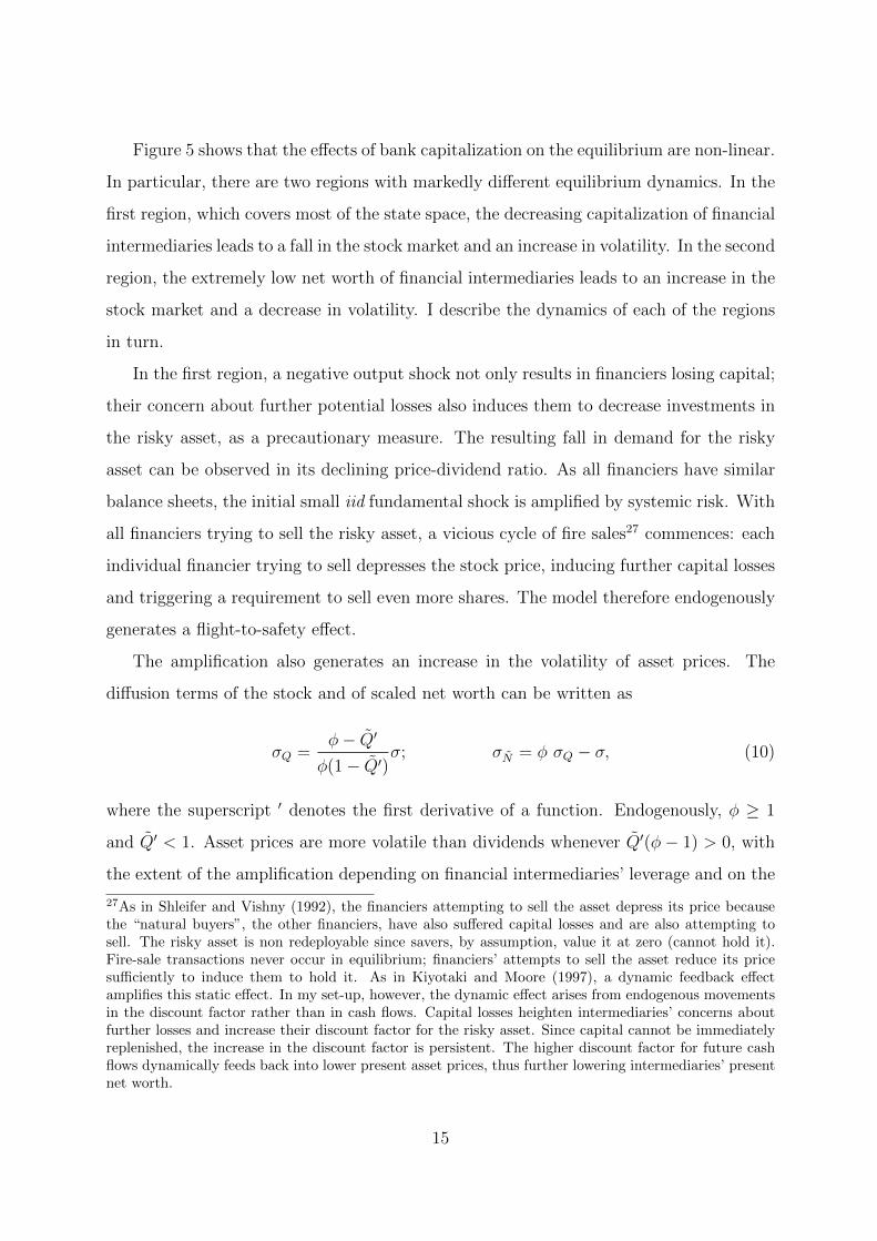
Figure 5 shows that the effects of bank capitalization on the equilibrium are non-linear.
In particular, there are two regions with markedly different equilibrium dynamics. In the
first region, which covers most of the state space, the decreasing capitalization of financial
intermediaries leads to a fall in the stock market and an increase in volatility. In the second
region, the extremely low net worth of financial intermediaries leads to an increase in the
stock market and a decrease in volatility. I describe the dynamics of each of the regions
in turn.
In the first region, a negative output shock not only results in financiers losing capital;
their concern about further potential losses also induces them to decrease investments in
the risky asset, as a precautionary measure. The resulting fall in demand for the risky
asset can be observed in its declining price-dividend ratio. As all financiers have similar
balance sheets, the initial small iid fundamental shock is amplified by systemic risk. With
all financiers trying to sell the risky asset, a vicious cycle of fire sales27 commences: each
individual financier trying to sell depresses the stock price, inducing further capital losses
and triggering a requirement to sell even more shares. The model therefore endogenously
generates a flight-to-safety effect.
The amplification also generates an increase in the volatility of asset prices. The
diffusion terms of the stock and of scaled net worth can be written as
σQ =φ− Q′
φ(1− Q′)σ; σN = φ σQ − σ, (10)
where the superscript ′ denotes the first derivative of a function. Endogenously, φ ≥ 1
and Q′ < 1. Asset prices are more volatile than dividends whenever Q′(φ− 1) > 0, with
the extent of the amplification depending on financial intermediaries’ leverage and on the
27As in Shleifer and Vishny (1992), the financiers attempting to sell the asset depress its price becausethe “natural buyers”, the other financiers, have also suffered capital losses and are also attempting tosell. The risky asset is non redeployable since savers, by assumption, value it at zero (cannot hold it).Fire-sale transactions never occur in equilibrium; financiers’ attempts to sell the asset reduce its pricesufficiently to induce them to hold it. As in Kiyotaki and Moore (1997), a dynamic feedback effectamplifies this static effect. In my set-up, however, the dynamic effect arises from endogenous movementsin the discount factor rather than in cash flows. Capital losses heighten intermediaries’ concerns aboutfurther losses and increase their discount factor for the risky asset. Since capital cannot be immediatelyreplenished, the increase in the discount factor is persistent. The higher discount factor for future cashflows dynamically feeds back into lower present asset prices, thus further lowering intermediaries’ presentnet worth.
15

reaction of the price-dividend ratio to changes in net worth.28 There is no amplification
only if financial intermediaries are not levered (φ = 1) or if the price-dividend ratio does
not react to changes in intermediary capital (Q′ = 0). In the first region, amplification
is positive since intermediaries are levered (φ > 1) and the price-dividend ratio falls
whenever intermediaries lose capital (Q′ > 0).
The equilibrium dynamics in this first region illustrate common characteristics of
financial crises. These dynamics change as further negative shocks push financial
intermediaries into the second region, where their capital is close to zero. Recall that, in
aggregate, the credit constraint takes the form ΩN ≥ 0. The tightness of the constraint
is determined by the balance of two opposing effects: losses of capital, reflected in a lower
N , induce increases in the value of capital, represented by a higher Ω.
In the first region, losses of capital outweigh the effect of increases in the value of capital
and tighten the constraint almost linearly. As financial intermediaries’ capital decreases
further and we enter the second region, the increase in the value of capital alleviates
the losses of capital and the constraint tightens more slowly. Intuitively, the higher
Sharpe ratio mitigates the incentives of financiers to walk away from poorly capitalized
financial intermediaries. This causes the price-dividend ratio to increase whenever there
are intermediary capital losses (Q′ < 0). In this case, equation (10) shows that capital
gains have a stabilizing effect on losses of net worth and dampen the volatility of asset
prices. The risky asset begins to mimic the risk-free one and, in the limit as net worth
approaches zero, the risky asset is locally risk less.29
28This emphasizes, as in Brunnermeier and Pedersen (2008), the interaction of market liquidity, i.e. theprice impact of transactions in the risky asset (Q′), and funding liquidity, i.e. the ability of financialintermediaries to raise capital for investment (φ).29This second region of the state space provides an endowment economy equivalent to financialdepressions, such as the one experienced in Japan starting in the early 1990s. Following the most acutephase of a crisis, where the stock market crashes and volatility increases, further losses of capital lead toa depression region. Here, stock prices are so high compared to dividends that risky investment returnsare low. Consequently, financiers are not able to quickly escape this region by accumulating net worththrough positive returns on investments. Figure 7 confirms the intuition by showing a fall in the driftand volatility of aggregate financial net worth. In the limit, as N ↓ 0, the drift approaches δQ and can beset arbitrarily close to zero, and the volatility goes to zero. Brunnermeier and Sannikov (2010) providea similar “area of attraction” in the low region of the state space. In my model, the main difference isthat the depression is caused solely by endogenous changes in the discount factor, while cash flows areexogenous.
16
Under the restriction δ = λ − ρ, the economy eventually converges to the Lucas
Economy equilibrium. Intuitively, financiers accumulate net worth sufficiently quickly
to reach a state where the entire supply of risky investments can be bought with the
financial intermediaries’ capital.30 In this state, the absence of leverage induces the
financial intermediaries’ capital to move one-for-one with stock prices, and financiers are
no longer concerned about losing their net worth. The equilibrium dynamics of this case
are illustrated in Figure 5. In contrast, under the restriction δ < λ− ρ financiers do not
converge to the frictionless equilibrium. In this case, deposits are always strictly positive
and the levered financiers are forever concerned about potential losses of net worth. The
resulting equilibrium dynamics are illustrated in Figure 6.
In both cases, the stochastic steady state31 is the point in Figure 7 where the drift of
scaled net worth equals zero. In the first case, the stochastic steady state is the upper
boundary of the state space: NSS = 1ρ . The limiting distribution of scaled net worth is
degenerate, with the entire probability mass concentrated at the stochastic steady state.
In the second case, the stochastic steady state is in the interior of the state space; the
stationary distribution of scaled net worth is reported in Figure 8. The distribution has
a fat left tail, since negative shocks are amplified more than positive shocks. Therefore,
while fundamental shocks are iid Gaussian, the banking economy suffers from endogenous
financial disasters.
The autarky model shows that agents are concerned about both fundamental
and financial risk. Furthermore, this concern creates lower demand for risky assets,
particularly during bad times, and an endogenous amplification of shocks. These elements
play a crucial role in the open economy that is analyzed in the next section.
30The balance of three effects regulates the asymptotic accumulation of aggregate net worth: financiersaccumulate capital at the rate of time preference ρ, start-up capital allocated to new financiers increasesaggregate net worth by δ, and net worth paid out by exiting financiers reduces aggregate net worth by λ.31The stochastic steady state is defined as the point to which the state variable converges if shocks arepossible but are not ever realized. This is in contrast to the most commonly analyzed deterministicsteady state, which is defined as the point of convergence if the model features no shocks (σ = 0).
17
III Open Banking Economy: Single World Tree
To understand the role of the US in the global financial architecture, I introduce a
simple model with two countries, Home and Foreign, which are symmetric other than
the extent to which their respective financial systems are developed. This stylized model
isolates the role of the asymmetry in the countries’ financial sectors and describes the
main result of this paper: the asymmetric risk sharing between the US and the RoW.
The empirical Facts 1-3 emerge from the implementation of this risk sharing.
The US, which acts as the key country in the global financial architecture, is
characterized by the greater extent of its financial development and, in particular, the
greater depth of its funding markets. This asymmetry is in the spirit of Kindleberger
(1965), Caballero et al. (2008), and Mendoza et al. (2009), who were among the first
to emphasize differences in financial development as a key driver of global imbalances.32
Eichengreen (2011, pages 17-33) emphasizes how the development of funding markets for
trade in New York in the 1920s was an important driver of the key country role switching
from the UK to the US.
One can think of a general form of the credit constraint, where financiers have different
abilities to divert assets or to walk away from their obligations. The less financiers are able
to divert assets or to walk away from their obligations, the greater financial development
is. This is meant to capture both the legal framework that is essential for the emergence
of financial markets, and the broader institutional and regulatory design that affects the
cost and efficiency of transactions in financial markets.
For simplicity I assume that Home financiers are unconstrained, while Foreign
financiers face the limited-liability constraint described in the previous section.33
32The assumption is also supported by the literature on comparative financial and institutionaldevelopment. Rajan and Zingales (1998), for example, motivate their empirical work, which assumesa frictionless financial market for the US, by noting that “capital markets in the United States are amongthe most advanced in the world”.33The choice of frictionless Home financial intermediation is one of convenience. It allows the model tobe analyzed with a single state variable. More generally, one can think of Home intermediaries facingfrictions, albeit lower than those faced by Foreign intermediaries. One-period and two-period versions ofthe model, which allow for frictions in both countries, yield similar qualitative results.
18
The global output of the sole good is generated by the process in equation (1); each
country is endowed with half of the output. Almost the entire set-up of each of the two
economies is identical to the autarky case, so I only describe the differences. I describe
the model for the Foreign country, and only specify the corresponding Home country
equations where necessary. Foreign variables are denoted by the superscript ∗.
Savers can only deposit funds with their domestic financial intermediaries; conse-
quently, they solve a problem identical to equation (2). This restriction emphasizes the
fact that private savings primarily enter the global financial system through domestic
financial institutions.34
In addition to raising deposits domestically and investing in the risky asset, financiers
can also lend and borrow in an international market for interbank35 loans. These
instantaneous interbank loans are promises to pay one unit of the consumption good. Both
interbank loans and deposits are risk free in equilibrium, so I directly use this outcome to
write their dynamics. The balance sheet of an individual financier is Qs∗ = n∗ + d∗ + b∗,
where b∗ is the amount that the financier has borrowed in the interbank market.
In a technical simplification36 from the autarky case, the exiting financiers have the
option to reinvest their net worth with the incoming financiers. Since financiers maximize
the value to their households of the intermediaries that they manage, they choose to
reinvest the net worth whenever Ω∗ > 1 and to pay it out whenever Ω∗ = 1, where
Ω∗, by analogy with the previous section, is the Foreign financier’s marginal value of
net worth. The representative financier problem is, therefore, equivalent to one for an
intermediary not paying any net worth out to the household until a stopping time
t′ ≡ inft : Ω∗(N∗(t)) = 1. After that point is reached, exiting financiers pay their net
34While off-shore accounts certainly exist, they are a small phenomenon compared to on-shore savings.35Literally, this market should be referred to as “inter-intermediary” rather than “interbank”. In practice,various types of financial intermediaries participate in the interbank funding market, so it is commonlyunderstood that it is not merely a market for banks.36This assumption allows for the simplification of the equilibrium risk sharing between Home and Foreignwithout altering the economic implications of the model. In particular, it allows the equilibrium to beexpressed as a function of a single state variable. See Appendix A for details.
19

worth to their households.37 The representative financier’s optimization problem is:
maxd∗(u),b∗(u),s∗(u)∞u=t
Λ∗(t)V ∗(t) = Et
[∫ ∞
t′Λ∗(u)e−λ(u−t′)λn∗(u)du
](11)
s.t. dn∗ = s∗(dQ+ Y dt)− r∗d d∗ dt− rb b∗ dt
V ∗ ≥ 0.
The Home financier’s problem is symmetric, but without the last constraint. I assume
that the start-up capital provided by households to new financiers is a function of the
stochastic steady state38 holdings of the risky asset in each country: S and S∗, respectively.
Consequently, new Home financiers receive δSQ and new Foreign financiers receive δS∗Q.
The aggregate net worth dynamics follow:
dN∗ = r∗dN∗dt+QS∗[(µQ − r∗d)dt+ σQdz] + δS∗dt
+B∗(r∗d − rb)dt.
An extra outflow of λN∗dt is detracted from the dynamics for all times after t′. The net
transfers from financiers to their households are:
Π∗ = −δS∗Q.
An extra inflow of λN∗dt is added to the dynamics for all times after t′.
The Foreign trade balance is the difference between the Foreign share of world output
and Foreign consumption. Foreign Net Foreign Assets (NFA) are the difference between
the wealth owned in Home by Foreign residents and the wealth owned in Foreign by Home
37For this to be an equilibrium, the state where Ω∗ = 1 needs to be absorbing. As with the autarky case,this is guaranteed by the restriction δ = λ − ρ, which is imposed in both this section and the next. SeeAppendices A and B for details.38The assumption is meant to capture the fact that the household uses both the current value of assetsand the long-run financial size of its country to judge how much start-up capital its new financiers needin order to operate. The specific functional form has been chosen to simplify the boundary analysis, anddoes not substantially affect the equilibrium.
20

residents.39 Finally, the change in Foreign NFA is the Foreign Current Account (CA).
Home definitions are symmetric. Thus, I have:
NX∗ ≡ Y
2− C∗; NFA∗ ≡
(S∗ − 1
2
)Q− B∗. (12)
The market clearing conditions are:
C + C∗ = Y ; S + S∗ = 1
B = −B∗; N∗ = S∗Q−D∗ − B∗.
A Optimal Consumption and Investment
The Home country has no frictions; consequently, the Home marginal value of net
worth is equal to one and the Home financiers’ value function takes the form V = n.
Foreign financiers instead value financial capital above one; as with the autarky case, their
value function is V ∗ = Ω∗(N∗)n∗. Since the Home and Foreign dynamic programming
problems of both savers and financiers are extensions of those in the autarky case, they
are reported in Appendix A. Here, I only include the corresponding Euler equations.
Lemma 3. The optimality conditions for Home savers and financiers imply that they
price assets according to:
0 = ΛY dt+ Et [d(ΛQ)] (13)
0 = Et [d(ΛDa)] (14)
0 = Et [d(ΛBa)] . (15)
The optimality conditions for Foreign savers and financiers imply that they price assets
39Proportionally to their capital, all financial intermediaries within each country are identical. Equilibriawith non-zero domestic interbank activity are possible, but are not materially different from theequilibrium where all interbank activity occurs across countries. Consequently, I focus on this lastequilibrium and therefore include the interbank loans in the NFA position.
21
according to:
0 = Λ∗Ω∗Y dt+ Et [d(Λ∗Ω∗Q)] (16)
0 = Et [d(Λ∗Da)] = Et [d(Λ
∗Ω∗Da)] (17)
0 = Et [d(Λ∗Ba)] = Et [d(Λ
∗Ω∗Ba)] , (18)
where Da is the deposit asset and Ba is the interbank asset.
Equations (13-15) show that the frictionless Home country only cares about
consumption risk: the Home representative agent prices assets as though it had
logarithmic preferences. By contrast, equations (16-18) show that the potentially
constrained Foreign country also cares about financial risk, in addition to consumption
risk. The Foreign representative agent discounts the stock more than an agent with
logarithmic preferences if, as is the case in equilibrium, it has low returns when financial
intermediaries have low capital. An immediate consequence of both deposits and
interbank loans being risk free is that, to prevent arbitrage, their rates of return are
equal: rb = rd = r∗d.
B Equilibrium
B.1 Open Lucas Economy
Consider a Lucas open endowment economy (Lucas (1982)) with two symmetric
countries, a single good generated by equation (1), and a representative agent with
logarithmic preferences in each country, both of whom can trade claims to the tree and a
risk-free bond. I refer to this economy in short as the Open Lucas Economy. If there are
no frictions in the Foreign financial system, then the equilibrium of my model is equivalent
to that of the Open Lucas Economy.40
Intuitively, the two countries are symmetric and the Foreign country is not affected by
frictions, so that agents only care about consumption risk. Consequently, the international
risk sharing and pricing equations reduce to the classic Lucas analysis. The equilibrium
40Details of the equilibrium are provided in Appendix A.
22

features of this economy are well known: symmetric equity portfolios, with each country
owning half of the shares; no trading in the risk-free interbank market; equal Home and
Foreign consumption state-by-state; and zero NFA, CA and NX. These results are a far
cry from the stylized facts of the global financial system in Facts 1-3.
B.2 Open Banking Economy
The equilibrium of the open economy with frictions is affected by the wealth
distribution, that is, the amount of capital inside the financial sector. However, only
Foreign financial intermediaries are affected by frictions; consequently, the key variable is
the fraction of the world’s wealth that is held as capital by Foreign financial intermediaries.
Proposition 2. The financier’s and saver’s optimization problems in the Home and
Foreign countries can be written in terms of a single state variable: the aggregate Foreign
financial sector net worth scaled by output N∗. Furthermore, the state variable is a strong
Markov process with dynamics given by
dN∗
N∗=
[(rd − λ− µ+ σ2) + φ∗(µQ − rd − σσQ) + δ
S∗Q
N∗
]dt+ (φ∗σQ − σ)dz
≡ µN∗dt+ σN∗dz,
where φ∗ ≡ S∗QN∗ . The equilibrium is characterized by a system of two coupled second-order
ODEs for the price-dividend ratio, Q(N∗), and the marginal value of Foreign net worth,
Ω∗(N∗):
0 = µQ − rd − σCσQ (19)
0 = µΩ∗ − σC∗σΩ∗ , (20)
where dCC = µCdt+ σCdz and dC∗
C∗ = µ∗Cdt+ σ∗
Cdz.
The system of ODEs has an intuitive interpretation; a formal analysis of the boundary
conditions and the numerical solution method is included in Appendix B. The ODE (19) is
a standard pricing equation: it shows that expected stock excess returns depend positively
on the covariance between Home consumption and stock returns. The ODE (20) ensures
23

that Foreign financiers and savers agree upon the price of risk-free deposits.41
The equilibrium allocation leads to an intuitive risk-sharing condition:
C∗
C=
Ω∗
ξ, (21)
where ξ is a scaling constant that depends on the initial conditions and is akin to the
relative weight of the Home country in a complete-market central-planner problem. The
risk sharing is asymmetric: an increase in the marginal value of Foreign financial capital
is associated with a relative increase in Foreign consumption over Home consumption. As
Ω∗ is counter-cyclical in equilibrium, this provides the foundations of the risk sharing that
underpins the global financial architecture.
In bad times, the consumption of the more financially developed country falls more
than that of the rest of the world.42 This occurs because Home financial intermediaries are
always able to achieve their desired investments in the risky asset by funding themselves
in the deposit or interbank markets; this makes them less concerned than Foreign financial
intermediaries about losses of capital. Consequently, the optimal risk sharing is for
Home financial intermediaries to increase their investments in the risky asset by levering
themselves in the international interbank market. Foreign financial intermediaries do
exactly the opposite: they accumulate precautionary long positions in risk-free interbank
deposits and decrease their investments in the risky asset. The portfolio implementation of
the risk sharing condition therefore generates the asymmetric Net Foreign Asset portfolio
of the Home and Foreign countries or, in actuality, of the US and the RoW (Fact 1 ).43
41In constrast to the autarky case, the restriction only imposes that the direct intra-temporal and inter-temporal effects of Ω∗ on the risk-free rate offset each other. In both ODEs, there are also indirect effectsof Ω∗, because consumption endogenously depends on Ω∗. See Appendix A for details.42The assumption that the Home financial system is frictionless, while simplifying the analysis, inevitablyproduces a Home consumption path that is volatile. In a quantitative analysis, however, it is theoreticallypossible to extend the model to a case where Home also faces frictions, albeit lower than those faced byForeign. In that case, the Home SDF would also feature an additional multiplicative term, like Ω, andthis extra degree of freedom would allow the main results of the paper to be generated with a lowervolatility of the Home consumption path.43The equilibrium portfolio can be interpreted in the language of comparative advantage, as applied totrade in assets (Helpman and Razin (1978), Svensson (1988)). In autarky, Home’s comparative advantagein financial markets results in higher Foreign than Home prices for “down state” Arrow securities. Oncethe two economies open for trade, Foreign will buy “down state” and sell “up state” Arrow securitiesfrom Home in order to achieve a safer portfolio overall.
24
The risk sharing condition has dynamic implications that emphasize the crucial role of
the Home country during financial crises. Figures 9-10 show the equilibrium of the Open
Banking Economy. Negative shocks cause capital losses in Foreign financial intermediaries
and a fall in the stock market. As in the autarky case, a vicious cycle of fire sales sets
in due to the systemic risk generated by the fact that all financial intermediaries hold
the same risky asset. As Foreign financial intermediaries try to sell the risky asset, they
further depress its price and, in turn, tighten their own credit constraints. Their increased
concern for their net worth also heightens the Foreign financial intermediaries’ desire to
invest with Home financial intermediaries in the risk-free interbank market. In turn, Home
financiers are willing to use the interbank funds that the Foreign financiers are providing
to buy the stock that Foreign financiers are trying to sell. However, Home financiers
require extra compensation for taking on this additional leveraged risk; this is achieved
through a combination of an increase in the expected stock excess returns and a decrease
in the interbank rate.
The global financial architecture is endogenously unstable. Since intermediaries are
levered and invest in the same risky asset, negative shocks are amplified. The model
endogenously generates a global flight to safety during crises, whereby Foreign financial
intermediaries demand Home intermediaries’ safe liabilities and Home’s external portfolio
loads more heavily on global risk. Part of the flight to safety occurs through a quantity
adjustment of countries’ portfolios, while the rest results from the price adjustment of
assets. In the limit, as Foreign financial intermediaries lose all their net worth,44 they
only own Home financial intermediaries’ safe liabilities.
The dynamic portfolio rebalancing of Home and Foreign is consistent with the
empirical evidence in Curcuru, Dvorak, and Warnock (2010), who find that the RoW
switches from equities to US safe assets precisely at times when the future performance
44The non-linear effects that occur in the autarky case when intermediaries’ net worth is close to zeroare no longer present. Their absence rests on the assumption that Home financiers are unconstrainedand can therefore always help clear the market for the risky asset, provided that it offers an appropriaterisk-return trade-off.
25
of these safe assets is poor compared to equities.45
In response to negative shocks, the static asymmetric Home and Foreign external
portfolios and the dynamic effects combine to generate a wealth transfer from Home to
Foreign (Fact 3 ). The wealth transfer supports the risk-sharing allocation by financing
the relatively higher Foreign consumption in these states of the world. This is evident
in Figure 9, where the value of the Home NFA portfolio falls in response to negative
shocks and Home and Foreign consumption shares and trade balances move in opposite
directions.46
On average, the Home country earns an expected compensation for the extra risk that
it takes on in the global financial system. This stream of income finances higher Home
consumption, and the Home country runs a trade deficit (Fact 2 ).47
The external adjustment of the US happens through both the traditional trade-balance
channel and unrealized valuation effects on its NFA. Consistent with the empirical
evidence of Gourinchas and Rey (2007), there are expected valuation effects on the NFA
portfolio. These valuation effects are generated in my model by time-varying risk premia.
In the long run, Foreign financial intermediaries eventually accumulate sufficient
capital to achieve their desired stock positions without raising deposits or borrowing or
lending in the interbank market. The restriction δ = λ− ρ ensures that this upper state
is absorbing. The stochastic steady state is one where Foreign financial intermediaries are
no longer concerned about losses of net worth. The Home country runs an asymptotic
trade deficit in the stochastic steady state. It does so not because it continues to earn
higher risk compensation, but because the asymmetric risk sharing that occurred before
reaching the steady state has allowed it to accumulate a positive NFA position.
45Curcuru et al. (2010) interpret the evidence in terms of bad timing of the purchase of US safe assetsfrom RoW investors. In a consistent but alternative explanation, I interpret the empirical evidence interms of risk compensation. RoW investors buy US safe assets during bad times because of their increasedconcern about fundamental and financial risk and their willingness to earn lower, or even negative, excessreturns as compensation for the safety of the asset.46In the figure, the trade balance is the difference between the country’s consumption share and the reddotted line at 0.5. If a country’s consumption share is more than 0.5, i.e. the country’s share of theendowment, then it runs a trade deficit.47In contrast to the Rueff (1971) interpretation of the US deficit as being “without tears”, I emphasizethat the US deficit is in fact financed by the “tears” of wealth transfers in bad states of the world.
26
In the data, the US NFA position is actually negative, but the US still runs a trade
deficit. The model helps to rationalize this seemingly puzzling outcome: despite being
a net debtor the US earns, on average, positive financial income since its assets, while
lower, are riskier than its liabilities. This income finances the trade deficit. The model,
however, cannot generate a long-run debtor position for the US because the stochastic
steady state is one where risk taking is symmetric.48 The stochastic steady state can be
interpreted as a “very long run” outcome in which the RoW financial development and
accumulation of capital make credit concerns irrelevant.
The model offers the view that some of the observed patterns in the data, including
the global imbalances, are the outcome of equilibrium risk sharing. However, it stresses
the substantial risks involved: the US benefits, on average, from positive financial income
on its external portfolio only because it takes greater risks. The model also makes clear
that the greater financial development of the US is not inconsistent with the 2008 crisis
and its negative effects on the US banking system. In the model, it is precisely because
US intermediaries are more efficient that they take more risk ex ante and, once a crisis
hits, suffer the most severe losses.
While the motivational evidence for this paper is focused on the US, the same
theoretical framework also sheds light on the role of the UK as the key country before the
First World War. London’s funding markets were then the deepest in the world; this was
a key factor in determining Britain’s financial dominance (Bagehot (1873)). My model is
related to Kindleberger’s (1965) hypothesis that the asymmetric external balance sheet
of Britain, with respect to its colonies, was due to differences in “demand for liquidity”
and did not necessarily represent a form of exploitation.49
My model also explains the global flight to safety toward the London funding markets,
described by Bagehot (1873) for the financial crises of the nineteenth century. In contrast
48An extension of the paper could introduce mean reversion in the state variable, as was done in theclosed economy, so that the US has a permanent advantage in financial intermediation. Logic suggeststhat this would allow the US, in extreme cases, to run both an asymptotic trade deficit and a negativeNFA position.49The similar claim of exploitation, or “exorbitant privilege”, that was later directed at the US by theFrench Finance Minister Valery Giscard d’Estaing, is often mentioned in connection with the stylized factsthat concern my main analysis. I have shown how this can be demystified as the outcome of equilibriumrisk sharing.
27

to the recent US history, however, Britain ran a sizable trade surplus at the time. In order
to reconcile this with my framework recall that, though it is the focus of my model, I am
not suggesting that financial development is the only determinant of the trade balance.
Instead, my framework indicates that the key country runs either more of a trade deficit
or less of a trade surplus than it would have otherwise done, if differences in the extent
of financial development were not present. This allows other facts, such as Britain’s
industrial base, to also play a role in determining the overall trade balance.
The above shows how a simple asymmetry in the global financial system can explain
the first three stylized facts (Facts 1-3 ) about the role of the US in the global financial
architecture and provide meaningful foundations for its economic analysis. To analyze
the missing stylized fact, the role of the US dollar as a reserve currency, I next extend the
open economy to feature an exchange rate by introducing differentiated goods.
IV Open Banking Economy: Two Trees
I maintain the assumption from the previous section that the Home financial system
is more developed than the Foreign one. In addition to applying this asymmetry to trade
in assets, I also let financial frictions affect international trade in goods by introducing
trade costs that are related to the state of the financial sector in each country. The
model emphasizes that shifts in demand for Home and Foreign goods are important to
understanding the dynamics of the exchange rate, particularly in times of global financial
stress. As will become clear, both financial sector frictions and trade costs play an
important role in determining these demand shifts.
There are two differentiated goods, one produced by Home and the other by
Foreign. The output of the two goods is given by processes
dY (t)
Y (t)= µ dt+ σ d(z(t);
dY ∗(t)
Y ∗(t)= µ dt+ σ∗ d(z(t), (22)
where σ = [σz 0], σ∗ = [0 σ∗z ], and (z is a vector of two independent standard Brownian
motions.
28

In both countries, agents have logarithmic preferences50 over a basket of the two goods,
with the Home and Foreign baskets given by, respectively:
C = CαHC
1−αF ; C∗ = C∗1−α
H C∗αF , (23)
where α ∈ [12 , 1) potentially allows for bias in each country’s preferences toward its
domestic good. I set a basket of the two goods, consisting of θ ∈ (0, 1) units of the Home
good and 1 − θ units of the Foreign good, as the numeraire. All prices are expressed in
this common unit.
To model trade costs I assume, for simplicity, iceberg transport costs: if one unit of
a good is shipped internationally, only 1τ units reach the destination, where τ ≥ 1. The
most literal interpretation of the model, and the one that I follow, is that the relative
variation in Home versus Foreign transport costs is due to the availability of credit. This
can be directly modeled within my framework. A less literal interpretation is that Home
and Foreign specialize in producing goods, the demand for which is affected differently
during global crises.51 Trade costs then need to be interpreted as reduced form demand
shifts according to economic conditions.52 As will become clear, both interpretations lead
to a Home shift in demand toward its own good during bad times; therefore, both have
similar equilibrium outcomes.
In keeping with the simplification that the Home country is unconstrained, I assume
that there are no transport costs for Home exports. Foreign export transport costs are a
function of the state of Foreign intermediaries. When intermediaries are well capitalized,
50In the models in Sections II and III, logarithmic preferences were mainly a matter of convenience. In thepresent section, logarithmic preferences permit one further simplification as agents have no desire to hedgetheir purchasing power risk (movements in the real exchange rate), thus allowing the model to be solvedwithout introducing the ratio of the two trees as a state variable (see Coeurdacier and Gourinchas (2008),Pavlova and Rigobon (2007)). The downside of this simplification is that the equilibrium portfolios donot reflect this extra hedging demand, which would occur under general CRRA preferences. The centralresults of the paper, however, focus on how the portfolios are affected by the demand to hedge financialrisk, which is not materially affected by the simplification to logarithmic preferences.51The production specialization could actually be due to the development of the financial system, as inAntras and Caballero (2009). This cannot be modeled directly here due to the assumption of exogenousendowments in the two countries.52An alternative set-up is one where the coefficient of Home bias is not constant. A shift in Home demandin bad times toward its own good can be represented by an α that depends positively on Ω∗. The mainimplications of the model for the exchange rate and global portfolios carry over to this set-up. For amodel of demand shocks that affect domestic bias see Pavlova and Rigobon (2010a).
29
Foreign exporters can easily access credit and trade costs are, therefore, low. By contrast,
in periods of financial stress, Foreign exporters’ access to credit dries up and trade costs
increase correspondingly. This is modeled in reduced form by: τ = Ω∗ε, where Ω∗, in line
with the previous section, is the Foreign marginal value of net worth and ε ≥ 0.
A long-standing literature has highlighted the importance of trade costs for
international finance (Samuelson (1954), Dumas (1992), Obstfeld and Rogoff (2001),
Coeurdacier (2009)), while a fast-growing literature is analyzing the collapse in trade
during the 2008 crisis. Chor and Manova (2011) find evidence that credit plays an
important role in explaining the dynamics of exports during the 2008 crisis: countries
that saw a more severe shutdown of their credit markets exported less to the US. Amiti
and Weinstein (2011) and Paravisini, Rappoport, Schnabl, and Wolfenzon (2011) also find
that credit conditions contribute to explaining the fall in exports for both Peru and Japan
during the 2008 crisis. Another strand of the literature has emphasized the importance
of both shifts in demand of tradables and global supply chains in explaining the 2008
collapse in trade (Eaton, Kortum, Neiman, and Romalis (2011), Levchenko, Lewis, and
Tesar (2010)).
Since the focus of this paper is not on explaining the collapse in trade during a crisis,
I want to clarify which elements of the empirical literature are relevant. I am interested
in the relative variation in demand, according to the state of the economy, between the
two countries for Home and Foreign goods. An overall symmetric increase in trade costs
or a fall in world demand, while quantitatively interesting, are not the focus of this paper.
Standard static optimization of the consumption baskets gives the Home and Foreign
demand for the two goods:53
CH = α( p
P
)−1
C; CF = (1− α)
(p∗τ
P
)−1
C (24)
C∗H = (1− α)
( p
P ∗
)−1
C∗; C∗F = α
(p∗
P ∗
)−1
C∗, (25)
where p and p∗ are the prices of the Home and Foreign good, respectively, and P and P ∗
are the prices of one unit of the Home and Foreign consumption baskets, respectively.
53See Appendix A.
30
The terms of trade (ToT) are defined as the ratio of Foreign to Home goods prices, such
that an increase in ToT represents a deterioration in the Home ToT. The real exchange
rate (E) is expressed as the Home price of Foreign currency and is given by the ratio of
Foreign to Home price indices.54 Thus, I have:
ToT ≡ p∗
p; E ≡ P ∗
P= (ToT )2α−1 τα−1. (26)
I denote the exchange rate dynamics by dEE = µEdt+σEd(z. Absent domestic bias (α = 0.5),
the exchange rate is only driven by movements in transport costs. In this case, an increase
in transport costs generates a Home currency appreciation. In the presence of domestic
bias (α > 0.5) and barring changes in transport costs, the real exchange rate and the ToT
are positively related.
Savers can only make deposits with domestic financial institutions. Deposits are
instantaneous promises to pay one unit of the domestic consumption basket. Deposits
are risk free for domestic agents because there is no default in equilibrium and deposits
pay the consumption basket. The saver’s problem is, therefore, identical to those in the
previous sections and is reported in Appendix A.
Financiers in each country can raise domestic deposits, invest in any of the two
stocks, and borrow or lend in an international interbank market. Interbank loans can be
denominated in either Home or Foreign currency and are instantaneous promises to pay
one unit of either the Home or Foreign consumption basket, respectively. The Foreign
financier’s balance sheet is s∗HQE + s∗FQ
∗ = n∗ + d∗ + b∗H + b∗F , where s∗H and s∗F are
the Foreign equity holdings of Home and Foreign stocks, Q and Q∗ are the prices of
the Home and Foreign stocks, both expressed in local currencies, and b∗H and b∗F are the
amounts borrowed in the interbank market in Home and Foreign currency, both expressed
in Foreign currency. As in the previous section, financiers who are selected to switch roles
are allowed to reinvest their net worth with incoming financiers.
54An increase in the exchange rate equates to a Home currency depreciation.
31

The Foreign financier’s optimization problem is:
maxd∗(u),b∗H(u),b∗F (u),s∗H(u),s∗F (u)∞u=t
Λ∗(t)V ∗(t) = Et
[∫ ∞
t′Λ∗(u)e−λ(u−t′)λn∗(u)du
](27)
s.t. dn∗ = s∗H
(d
(Q
E
)+
pY
P ∗ dt
)+ s∗F
(dQ∗ +
p∗Y ∗
P ∗ dt
)+
−r∗d d∗ dt− (rb dt− dE) b∗H − r∗b b∗F dt
V ∗ ≥ 0,
where Λ∗ ≡ e−ρt 1C∗ and t′ ≡ inft : Ω∗(N∗(t)) = 1. The Home financier’s problem is
entirely similar, but without the last constraint.
As a generalization of the previous section, I assume that the start-up capital provided
by households to new financiers is a function of the stochastic steady state holdings of
the two stocks: S∗H , S
∗F. Consequently, new Home financiers receive δ[SHQ + SFEQ∗]
and new Foreign financiers receive δ[S∗H
QE + S∗
FQ∗].
The definitions of the Foreign trade balance and the NFA are generalizations of those
in equation (12):
NX∗ ≡ p∗
P ∗Y∗ − C∗; NFA∗ ≡ S∗
H
Q
E − SFQ∗ − B∗
H − B∗F .
The market clearing conditions are:
CH + C∗H = Y ; τCF + C∗
F = Y ∗
SH + S∗H = 1; SF + S∗
F = 1
BH = −EB∗H ; BF = −EB∗
F
N∗ = S∗H
Q
E + S∗F Q∗ −D∗ − B∗
H − B∗F .
A Optimal Consumption and Investment
In line with Section III.A, the Home financier’s value function takes the form V = n
and that of the Foreign financier takes the form V ∗ = Ω∗(N∗)n∗. The Home and Foreign
dynamic programming problems of both savers and financiers and the corresponding Euler
32
equations, which are extensions of those in Lemma 3, are reported in Appendix A. Here I
want to emphasize the Home financier’s Euler equation for the optimal trade-off between
interbank loans denominated in Home and Foreign currency:
r∗b − rb + µE = −Covt
(dΛ
Λ,dEE
)= σC σT
E , (28)
where the superscript T denotes the vector transpose. The Home currency safety premium,
the compensation required to invest in Foreign currency by shorting Home currency, is
determined by the covariance between Home consumption and the real exchange rate. If
the Home currency appreciates (↓ E) whenever Home consumption is low, then the Home
currency has a positive safety premium. Intuitively, Home interbank loans are safer than
their Foreign counterparts because they pay more in bad states of the world.
Since deposits and interbank loans are risk-free in their local currency, no arbitrage
implies that rb = rd and r∗b = r∗d.
B Equilibrium
B.1 Cole and Obstfeld Economy
In their classic analysis of the irrelevance of asset markets for international risk sharing,
Cole and Obstfeld (1991) show that in an open economy with differentiated goods, agents
with logarithmic preferences, and no trade costs, the central-planner’s allocation can be
achieved even without trade in asset markets.55 I refer in brief to this economy as the
Cole and Obstfeld Economy.
If there are no frictions, then the equilibrium of my model reduces to that of the Cole
and Obstfeld Economy. Intuitively, if Foreign financiers face no frictions then: Ω∗(t) = 1,
so that the Euler equations and the demand equations for goods simplify to those in the
frictionless world of Cole and Obstfeld.55This occurs because the endogenous response of the ToT to supply shocks to the two goods is sufficientto implement the international wealth transfers that support the central planner’s consumption allocation.
33
As is well known, the Cole and Obstfeld equilibrium features: perfectly correlated
Home and Foreign stock markets, symmetric aggregate stock market portfolio holdings,56
zero holdings of risk-free bonds,57 equal consumption state by state, zero NX, and
indeterminate58 NFA and CA. The exchange rate is either constant (α = 0.5) or positively
related to the ToT (α > 0.5). These results are a far cry from the stylized facts in Facts
1-4.
B.2 Open Banking Economy: Two Trees
In line with Section III.B.2, the equilibrium is characterized by a single state variable,
the aggregate scaled59 net worth of Foreign financiers, and a system of three ODEs.
Proposition 3. The equilibrium is characterized by a system of three coupled second-order
ODEs for the Home price-dividend ratio, Q(N∗), the Foreign price-dividend ratio, Q∗(N∗),
and the marginal value of Foreign net worth, Ω∗(N∗):
0 = µQ − rb − σCσTQ (29)
0 = µQ∗ + µE + σEσTQ∗ − rb − σC(σQ∗ + σE)
T (30)
0 = µΩ∗ − σC∗σTΩ∗ . (31)
The risk sharing allocations are a generalization of equation (21):
P ∗C∗
PC=
Ω∗
ξ(32)
56Individual stock market positions are indeterminate since the two stocks are perfectly correlated, buteach country’s holding of the aggregate stock market is determinate.57In my setting there are zero holdings in the interbank market, which is the equivalent of the risk-freeinternational bonds in Cole and Obstfeld (1991), but the deposit market is still active. However, notethat without frictions the trading in the deposit market is merely a matter of internal accounting betweensavers and financiers in each country, without any real effects. In this sense the Cole and Obstfeld (1991)result on the irrelevance of international asset markets for risk sharing holds in my set-up when there areno frictions.58The NFA indeterminacy is a consequence of the indeterminacy of the portfolio holdings of each stock.The CA is indeterminate because it is the change in NFA.59Consistently with the previous sections, I normalized by the value of world output expressed in theappropriate currency. Consequently, Home variables are scaled by pY+p∗Y ∗
P and Foreign variables bypY+p∗Y ∗
P∗ .
34

C∗H =
(1− α)Ω∗
αξ + (1− α)Ω∗Y ; CH =αξ
αξ + (1− α)Ω∗Y (33)
C∗F =
αΩ∗
(1− α)ξ + αΩ∗Y∗; CF =
1
τ
(1− α)ξ
(1− α)ξ + αΩ∗Y∗. (34)
Equation (32) is the risk sharing condition that underpins the global financial architecture.
It states that the value of Foreign consumption increases relative to that of Home whenever
the Foreign marginal value of net worth increases. Since in equilibrium Ω∗ is counter-
cyclical, this occurs in bad economic times.
The terms of trade and the exchange rate can also be understood in terms of
movements in Ω∗. The risk sharing conditions above and the definitions in equation
(26) imply that:
ToT =ξ(1− α) + αΩ∗
αξ + (1− α)Ω∗Y
Y ∗ ; E = (ToT )2α−1 Ω∗ε(α−1).
The ToT are determined by two effects. Movements in the ratio of the two trees affect
the ToT by altering the relative supply of the two goods. If the Home good becomes
relatively more scarce, then it also becomes relatively more expensive, and the Home
ToT improve. This effect is present irrespective of domestic bias. In addition, if there is
domestic bias (α > 0.5), an increase in Ω∗ weakens the Home ToT. This happens because
an increase in Ω∗, according to equation (32), increases the relative consumption of Foreign
residents. If the preferences of agents are biased toward the Foreign good (α > 0.5), this
induces a relative increase in the demand for the Foreign good. To clear the market,
its price increases relative to the Home good. If these agents have no preference bias
(α = 0.5), then the ToT are unaffected.
The exchange rate is determined by the combination of three effects. The first two
effects derive from the movement in the ToT analyzed above. If α = 0.5, these two
effects disappear because the Home and Foreign consumption baskets are identical and
movements in the ToT have no effect on the exchange rate. The third effect is caused by
variations in trade costs. An increase in Ω∗ induces an increase in Foreign export costs.
The higher costs increase the prices Home residents pay for the Foreign good (see equation
(34)), thus relatively increasing the Home price index and causing the Home currency to
35

appreciate.60 The effect is absent in the limit α ↑ 1, because countries only consume their
own good and never export their good.
The effects on the ToT and exchange rate can be understood in terms of the classic
Keynes and Ohlin debate on the “transfer problem”.61 In my setting, an increase in Ω∗
is associated with a wealth transfer from Home to Foreign. The reaction of the exchange
rate depends on what Foreign (Home) residents do with the additional (reduced) wealth.62
Traditional international macroeconomic models predict that a transfer of wealth from
the US to the RoW results in a US dollar depreciation. This prediction derives from the
second channel described above: the increased relative demand for RoW goods due to the
relatively higher wealth of RoW residents. If the US, in fulfilling its role as the key country
in the global financial architecture, takes more risk in equilibrium than other countries,
the wealth transfer occurs during bad economic times (Fact 3 ). Traditional models would
then predict a US dollar depreciation in such times.63 If this were the case, however,
the US dollar would be a risky asset for RoW residents, since it would pay low in bad
states of the world. The role of the US dollar as a reserve currency (Fact 4 ), therefore, is
inconsistent with this traditional mechanism. This is the “reserve currency paradox”: the
key country’s currency appreciates during a crisis despite the country suffering heavier
wealth losses relative to other countries.
The model rationalizes this paradox by noting that in normal times, or even for mild
negative shocks, the combination of the various effects produces an ambiguous exchange-
rate response. However, for sufficiently large adverse shocks, such as global crises, the
relative shift in demand toward the Home good, caused by an increase in τ , dominates and
60The trade cost does not affect the ToT, because in a Cobb-Douglas aggregator the unit elasticity ofdemand of the two goods implies that the wealth and substitution effects originating from trade costsexactly offset each other. In a more general CES aggregator, one could argue that an increase in Foreigntrade costs reduces Home demand for Foreign goods and tends to improve the Home terms of trade.61Following World War I, the Dawes committee imposed reparation payments from Germany to France.Keynes argued that, in addition to the primary burden of the wealth transfer, Germany would suffer asecondary burden due to the deterioration in its terms of trade (Keynes (1929)). Ohlin, on the contrary,argued that no secondary burden would occur as long as French people spent the transfer on Germangoods (Ohlin (1929)).62The effect of trade costs on the “transfer problem” was analyzed by Samuelson (1952, 1954).63This is reminiscent of “Triffin’s dilemma”. Triffin (1960) postulated that in running large trade deficitsdue to its effort to provide the world reserve currency, the US would suffer heavier losses, and potentiallya run on its currency, during global crises.
36
the Home currency appreciates. This non-linearity allows for rich exchange rate dynamics.
While it is consistent with the traditional view, with the exchange rate behaving much
as predicted by traditional models in normal times, it extends this mechanism in order to
make sense of the behavior of the exchange rate during extreme events.
Figures 11-12 isolate the role of the Home currency as a global safe asset by presenting
the equilibrium of the model under no domestic bias (α = 0.5). In this case, the exchange
rate is entirely driven by movements in trade costs. Since the Home currency appreciates
whenever intermediaries lose capital, it provides a hedge for the global financial system.
Correspondingly, Figure 12 shows that the Home currency has a safety premium (Fact
4 ): global financial intermediaries are willing to earn negative expected excess returns as
compensation for holding this safe currency.
Figure 11 shows how the equilibrium risk sharing allocation between Home and Foreign
is implemented via the financial intermediaries’ portfolios. First, note that for the case
where α = 0.5 the returns of the two stocks in the same currency are perfectly correlated,
as in Cole and Obstfeld (1991), because changes in the ToT exactly offset the dividend
shocks.64 Therefore, I focus on intermediaries’ holdings of the aggregate world stock
market. The insight from Cole and Obstfeld (1991) on the relevance of asset markets
for risk sharing has one further implication for my model (for the case α = 0.5): despite
the presence of two sources of fundamental risk, the two dimensional Brownian motion
(z, two independent assets are sufficient to achieve the equilibrium risk sharing.65 Figure
11 presents the case where intermediaries can trade the world stock market and lend or
borrow in the Home-currency interbank market.
Foreign intermediaries invest in the risky asset, the stock market, and hold
precautionary long positions in Home currency in the interbank market. Following a
negative shock, Foreign intermediaries lose capital and their heightened concern for further
64See Appendix A for details. The drawback is that in this case, as in Cole and Obstfeld (1991), the NFAand CA are indeterminate. See Pavlova and Rigobon (2007, 2010a,b) for a discussion of how the resultof Cole and Obstfeld (1991) affects a set-up with domestic bias and demand shocks.65International markets’ completeness requires three independent traded assets. Recall from SectionIV.B.1 that in the Cole and Obstfeld Economy international asset markets are completely unnecessaryto implement the risk sharing. Here the difference is that international asset markets are necessary toimplement the asymmetric risk sharing, but an international asset market structure that falls short ofthe complete one is sufficient for the implementation.
37
losses leads to a fall in their investments in the risky asset and an increased demand for
the Home currency. This global flight toward the Home currency leads to an increase in
its safety premium through both an expected Home currency depreciation and a more
pronounced fall in the Home interest rate than in the Foreign one. Even in the limit, as
Foreign intermediaries lose all capital, their long positions in Home currency allow them
to hedge the risk deriving from their long stock positions and, in contrast with Section
III.B.2, Foreign intermediaries maintain a long position in the stock.66
I offer a view of the international role of the US dollar as a reserve currency based
on risk. This contrasts with previous models of the key currency that had focused on its
role as a vehicle currency, that is, a medium of exchange, in international transactions
(Krugman (1980), Matsuyama, Kiyotaki, and Matsui (1993)).
The model provides a rationale for the “Global Saving Glut”, the hypothesis
formulated by Bernanke (2005) that the RoW demand for US safe assets lowered US
interest rates and contributed to large US trade deficits. In the spirit of Caballero
and Krishnamurthy (2009), the model stresses how Home safe liabilities are demanded
by global financial intermediaries as a precautionary investment. More technically, the
combination of the Home safe asset and the risky assets, the two stocks, allows Foreign
intermediaries to replicate the Foreign risk-free asset, which might not be directly available
to trade. Following negative shocks, the increased Foreign demand for the Home safe
asset accentuates the fall in the Home risk-free rate. In contrast to the previous papers,
however, I emphasize the importance of the exchange rate. Even the safest US assets, such
as Treasuries and short term liabilities of the banking system, would not be particularly
safe for RoW investors if the US dollar were to systematically depreciate during crises.67
A dimension along which the model could be extended is the heterogeneity of
66The equilibrium for the case that allows financial intermediaries to trade the stocks and the Foreign-currency denominated interbank deposits features identical allocations and asset prices. The portfolios,however, are different: Foreign intermediaries are long the stocks and lend in the interbank market in theForeign currency. As the Foreign intermediaries lose capital they decrease their positions in the stock andincrease their lending in the Foreign currency. In the limit, as Foreign intermediaries have no net worth,they own no stocks and only lend in the Foreign currency. These portfolios are not consistent with thoseobserved in the data (Fact 1 ).67Notable exceptions are countries with currencies that are (quasi-)pegged to the US dollar, such as China.The accumulation of precautionary reserves in US dollars, however, extends well beyond countries withpegged currencies.
38
financial intermediaries. Bernanke, Bertaut, DeMarco, and Kamin (2011) and Shin (2011)
provide empirical evidence that there is heterogeneity in the portfolios of RoW financial
intermediaries. For example, the evidence suggests that intermediaries based in Asia and
other emerging markets have long positions in US safe assets, while some of the larger
European banks are both funding themselves in the US and investing these funds in a
wider spectrum of US assets, including bond and equities. In short, these European
intermediaries are providing off-shore financial intermediation to the US, which Bernanke
et al. (2011) and Shin (2011) suggest is related to lower capital requirements for European
banks.68
Since the focus of my paper is on explaining the aggregate US international position,
I have grouped the RoW intermediaries into one homogenous class. This simplification
allows the model to sharpen its focus on aggregate flows, and leaves it to future research
to also model the heterogeneity of the RoW intermediaries.
V Conclusion
A simple asymmetry in the global financial system, heterogeneity in financial
development, can rationalize the economic role of the US in the global financial
architecture. I have shown how the greater depth of financial development of the US
leads to its role as the global risk taker with respect to both fundamental and financial
risk. The four stylized facts that motivated my analysis emerge as consequences of the
asymmetric risk taking that characterizes the global financial architecture.
The model not only provides a theoretical framework that jointly makes sense of these
facts; its main contribution is to have done so by providing the underlying economic
foundations through the explicit modeling of financial intermediation and its frictions.
These foundations have highlighted the risks that affect the global financial system, as
well as the costs and rewards for each country. The tractability of the foundations and
the almost analytical solution method provide a base for future research.
68This is a form of regulatory or tax arbitrage. Similarly, one could argue that Switzerland and Singapore,countries with high financial development, also provide off-shore intermediation. The role of thesefinancial centers in the global financial architecture seems to be mainly related to these regulatory andtax advantages.
39
ReferencesAlvarez, F. and U. J. Jermann (2000). Efficiency, equilibrium, and asset pricing with riskof default. Econometrica 68 (4), 775–797.
Amiti, M. and D. E. Weinstein (2011). Exports and financial shocks. Quarterly Journalof Economics .
Antras, P. and R. J. Caballero (2009). Trade and capital flows: A financial frictionsperspective. Journal of Political Economy 117 (4), pp. 701–744.
Bagehot, W. (1873). Lombard Street: A Description of the Money Markets. Henry S.King and Co., London.
Bernanke, B. (2005). The global saving glut and the U.S. current account deficit.Sandridge Lecture, Virginia Association of Economists.
Bernanke, B., C. Bertaut, L. DeMarco, and S. Kamin (2011). International capital flowsand the returns to safe assets in the United States, 2003-2007. International FinanceDiscussion Papers, Board of Governors of the Federal Reserve.
Bernanke, B. and M. Gertler (1989). Agency costs, net worth, and business fluctuations.American Economic Review 79 (1), 14–31.
Bernanke, B., M. Gertler, and S. Gilchrist (1999). The financial accelerator in aquantitative business cycle framework. Volume 1 of Handbook of Macroeconomics,Chapter 21, pp. 1341–1393. Elsevier.
Brunnermeier, M., T. Eisenbach, and Y. Sannikov (2010). Macroeconomics with financialfrictions: A survey. In Proceedings of the Econometric Society World Congress.
Brunnermeier, M. and L. J. Pedersen (2008). Market liquidity and funding liquidity.Review Finanial Studies , 2201–2238.
Brunnermeier, M. and Y. Sannikov (2010). A macroeconomic model with a financialsector. Unpublished manuscript, Princeton University .
Caballero, R., E. Farhi, and P. O. Gourinchas (2008). An equilibrium model of globalimbalances and low interest rates. American Economic Review 98 (1), 358–93.
Caballero, R. and A. Krishnamurthy (2009). Global imbalances and financial fragility.American Economic Review: Papers & Proceedings 99, 584–88.
Chor, D. and K. Manova (2011). Off the cliff and back? Credit conditions andinternational trade during the global financial crisis. Journal of InternationalEconomics .
Coeurdacier, N. (2009). Do trade costs in goods market lead to home bias in equities?Journal of International Economics 77 (1), 86–100.
Coeurdacier, N. and P. O. Gourinchas (2008). When bonds matter. Unpublishedmanuscript, UC Berkeley, Sciences Po.
Cole, H. L. and M. Obstfeld (1991). Commodity trade and international risk sharing:how much do financial markets matter? Journal of Monetary Economics 28 (1), 3–24.
Cox, J., J. Ingersoll, and S. Ross (1985). An intertemporal general equilibrium model ofasset prices. Econometrica, 363–384.
Curcuru, S. E., T. Dvorak, and F. E. Warnock (2008). Cross-Border returns differentials.Quarterly Journal of Economics 123 (4), 1495–1530.
Curcuru, S. E., T. Dvorak, and F. E. Warnock (2010). Decomposing the U.S. externalreturns differential. Journal of International Economics 80 (1), 22 – 32.
Despres, E., C. Kindleberger, and W. Salant (1966). The dollar and world liquidity: aminority view. The Economist (February 5), 526–529.
Duffie, D. (2001). Dynamic Asset Pricing Theory, Third Edition. (3 ed.). PrincetonUniversity Press.
Dumas, B. (1992). Dynamic equilibrium and the real exchange rate in a spatially separated
40

world. Review of financial studies 5 (2), 153.Eaton, J., S. Kortum, B. Neiman, and J. Romalis (2011). Trade and the global recession.National Bureau of Economic Research Working Paper Series No. 16666.
Eichengreen, B. (2011). Exorbitant Privilege: the rise and fall of the Dollar and the futureof the international monetary system. Oxford University Press.
Fostel, A. and J. Geanakoplos (2008). Leverage cycles and the anxious economy. AmericanEconomic Review 98 (4), 1211–44.
Garleanu, N. and L. Pedersen (2011). Margin-based asset pricing and deviations from thelaw of one price. Review of Financial Studies 24 (6), 1980.
Gertler, M. and P. Karadi (2011). A model of unconventional monetary policy. Journalof Monetary Economics 58 (1), 17 – 34.
Gertler, M. and N. Kiyotaki (2010). Financial intermediation and credit policy in businesscycle analysis. Volume 3 of Handbook of Monetary Economics, Chapter 11, pp. 547–599.Elsevier.
Gourinchas, P. O., N. Govillot, and H. Rey (2010). Exorbitant privilege and exorbitantduty. Unpublished manuscript, UC Berkeley, LBS and Ecole de Mines.
Gourinchas, P. O. and H. Rey (2007). International financial adjustment. Journal ofPolitical Economy 115 (4), 665–703.
Gourinchas, P. O., H. Rey, and K. Truempler (2011). The financial crisis and thegeography of wealth transfers. Unpublished manuscript, UC Berkeley, London BusinessSchool .
Hassan, T. (2010). Country size, currency unions, and international asset returns.Unpublished manuscript, University of Chicago GSB .
He, Z. and A. Krishnamurthy (2010). Intermediary asset pricing. Unpublished manuscript,University of Chicago and Northwestern University .
Helpman, E. and A. Razin (1978). A theory of international trade under uncertainty.Academic Press, NY.
Karlin, S. and H. M. Taylor (1981). A Second Course in Stochastic Processes. New York:Academic Press.
Keynes, J. (1929). “The german transfer problem”; “The reparation problem: adiscussion. II. A rejoinder”;“Views on the transfer problem. III. A reply”. The EconomicJournal .
Kindleberger, C. (1965). Balance-of-payments deficits and the international market forliquidity. Number 46. International Finance Section, Princeton University.
Kiyotaki, N. and J. Moore (1997). Credit cycles. The Journal of Political Economy 105 (2),211–248.
Kiyotaki, N. and J. Moore (2008). Liquidity, business cycles, and monetary policy.Unpublished manuscript, Princeton University and Edinburgh University .
Krugman, P. R. (1980). Vehicle currencies and the structure of international exchange.Journal of Money, Credit and Banking 12, 513–526.
Krugman, P. R. (1984). The international role of the dollar: Theory and prospect. NBERAnnual: Exchange rate theory and practice, 261–278.
Kurlat, P. (2009). Lemons, market shutdowns and learning. Unpublished manuscript,Stanford University .
Lane, P. and G. Milesi-Ferretti (2007). The external wealth of nations mark II: revised andextended estimates of foreign assets and liabilities, 1970-2004. Journal of InternationalEconomics 73 (2), 223 – 250.
Lane, P. and J. Shambaugh (2010). Financial exchange rates and international currencyexposures. American Economic Review 100 (1), 518–540.
Levchenko, A. A., L. T. Lewis, and L. L. Tesar (2010). The collapse of internationaltrade during the 2008-2009 crisis: In search of the smoking gun. National Bureau of
41
Economic Research Working Paper Series No. 16006.Lucas, R. (1978). Asset prices in an exchange economy. Econometrica, 1429–1445.Lucas, R. (1982). Interest rates and currency prices in a two-country world. Journal ofMonetary Economics 10 (3), 335–359.
Lustig, H., N. Roussanov, and A. Verdhelan (2010). Countercyclical currency risk premia.Unpublished manuscript, UCLA, Wharton and MIT .
Maggiori, M. (2010). The U.S. dollar safety premium. Unpublished manuscript, UCBerkeley .
Martin, I. (2011). The forward premium puzzle in a two country world. Unpublishedmanuscript, Stanford University .
Matsuyama, K., N. Kiyotaki, and A. Matsui (1993). Toward a theory of internationalcurrency. The Review of Economic Studies 60 (2), 283–307.
Mendoza, E. G., V. Quadrini, and J. V. Rıos Rull (2009). Financial integration, financialdevelopment, and global imbalances. Journal of Political Economy 117 (3), pp. 371–416.
Obstfeld, M. and K. Rogoff (2001). The six major puzzles in international macroeco-nomics: is there a common cause? Unpublished manuscript, UC Berkeley and HarvardUniversity .
Ohlin, B. (1929). “The reparation problem: A discussion. I. Transfer difficulties, real andimagined”; “Mr. Keynes’ views on the transfer problem. II. a rejoinder”. EconomicJournal .
Øksendal, B. (2003). Stochastic differential equations: an introduction with applications(6 ed.). Springer.
Paravisini, D., V. Rappoport, P. Schnabl, and D. Wolfenzon (2011). Dissecting the effectof the credit supply on trade: evidence from matched credit-export data. Unpublishedmanuscript, Columbia GSB, NYU Stern.
Parlour, C., R. Stanton, and J. Walden (2011). Financial flexibility, bank capital flows,and asset prices. Unpublished manuscript UC Berkeley .
Pavlova, A. and R. Rigobon (2007). Asset prices and exchange rates. Review FinancialStudies 20 (4), 1139–1180.
Pavlova, A. and R. Rigobon (2010a). An asset-pricing view of external adjustment.Journal of International Economics 80 (1), 144 – 156.
Pavlova, A. and R. Rigobon (2010b). Equilibrium portfolios and external adjustmentunder incomplete markets. Unpublished manuscript LBS and MIT .
Rajan, R. G. and L. Zingales (1998). Financial dependence and growth. AmericanEconomic Review 88 (3), pp. 559–586.
Rueff, J. (1971). The monetary sin of the West. London: Macmillan.Samuelson, P. (1952). The transfer problem and transport costs: the terms of trade whenimpediments are absent. The Economic Journal 62 (246), 278–304.
Samuelson, P. (1954). The transfer problem and transport costs, II: analysis of effects oftrade impediments. The Economic Journal 64 (254), 264–289.
Shin, H. (2011). Global banking glut and loan risk premium. Mundell-Fleming Lecture,International Monetary Fund .
Shleifer, A. and R. Vishny (1992). Liquidation values and debt capacity: A marketequilibrium approach. Journal of Finance, 1343–1366.
Simsek, A. (2009). Belief disagreements and collateral constraints. Unpublishedmanuscript, Harvard University .
Svensson, L. E. O. (1988). Trade in risky assets. American Economic Review 78 (3),375–394.
Triffin, R. (1960). Gold and the dollar crisis; the future of convertibility. Yale UniversityPress, New Haven.
42

Appendix A: Proofs
Lemma 1. Given the conjecture that the saver’s value function only depends on scaleddeposits and scaled net transfers, U(D, Π), the optimization problem is solved by thefollowing Hamilton-Jacobi-Bellman (HJB) equation:
0 = supC
log(C)dt− ρU(D, Π)dt+ Et
[dU(D, Π)
]
s.t. dD = D(rd − µ+ σ2)dt+ (Π− C)dt− Dσdz
dΠ = Nλ(rd − λ) + Q[λ(µQ + δ − rd)− δµQ − σσQ(λ− δ)] +
+Π(σ2 − µ) + δdt+ [QσQ(λ− δ)− Πσ]dz.
The first order condition (FOC) is: C−1 = U ′D, where the left hand side (LHS) is the
first derivative of U with respect to the scaled deposits. The verification that the valuefunction only depends on D, Π follows by substituting the FOC back into the HJBequation, and from the fact that:
N =Π+ δD
λ− δ
Q =Π+ λD
λ− δ,
and from the fact that Q, µQ, σQ, rd are going to only be functions of N and can thereforebe recovered by knowing D, Π. The sufficiency of the HJB equation for the solutionof the optimization problem follows standard steps from the Verification Theorem.69 Anexplicit verification is omitted here and in the following proofs.
To establish the claim that −rd dt = Et
[dΛΛ
], I employ the approach in Cox, Ingersoll,
and Ross (1985). I take the difference between two expressions. The first expression is
obtained by using the FOC above to write Λ = e−ρt U′DY , and by applying Ito’s lemma to
this function. The second expression is obtained by taking the partial derivative of theHJB equation above with respect to D and by then multiplying it by e−ρt
Y . Taking thedifference between the two expression establishes, after tedious but standard algebra, theclaim.
Lemma 2. Given the conjecture that the financier’s value function depends on aggregatescaled net worth and the individual financier’s net worth, V (N , n), the optimizationproblem is solved by the following HJB equation:
0 = sups
λΛλndt+ Et
[d(ΛλV (N , n))
]+ χ(t)dt V (N , n)
s.t. dn = s(dQ+ Y dt)− rd d dt
dN =[N(rd − λ− µ+ σ2) + Q(µq − rd + δ − σσQ)
]dt+ (QσQ − Nσ)dz,
69See Øksendal (2003, page 241).
43
where χ is the Lagrange multiplier. The FOC is:
µQ − rd = σCσQ − σΩσQ. (35)
When substituting the FOC back into the HJB equation, I obtain a restriction that thefunction Ω has to satisfy for the conjecture of the value function to be valid:
0 = λ(1− Ω)
Ω+ µΩ − σCσΩ. (36)
As long as Q, µQ, σQ, rd only depend on N in equilibrium, then the conjecture that Ωonly depends on N is verified.
Using the saver’s Euler equation in equation (4) and equation (36), algebraicmanipulations yield the result in equation (6). The additional use of the financier’s FOCyields the result in equation (5).
Proposition 1. The proofs of Lemma 1 and 2 state that to solve the saver’s and financier’soptimization problems one only needs to know the variable N , as long as Q, µQ, σQ, rdonly themselves depend on that variable. The saver’s Euler equation, equation (4), andthe market clearing condition C = Y together imply that the deposit rate is constant inequilibrium and is given by rd = ρ+ µ− σ2. Applying Ito’s lemma to Q = Q
Y and to the
conjecture Q(N) and matching the corresponding drift and diffusion terms yields:
µQ(t) =1 + Q[µ+ Q′(δ − µ− ρ)] + NQ′(ρ− λ)
Q(1− Q′)+
(Q− N)Q′σ2
Q(1− Q′)+
(Q− N)2Q′′σ2
2Q(1− Q′)3
σQ(t) =Q− NQ′
Q(1− Q′)σ.
Substituting these expressions into the financier’s FOC (equation (35)) yields the ODEfor Q(N), reported in implicit form in equation (9), thus verifying that N is the onlystate variable. The proof that the state variable is a strong Markov process follows fromits dynamics in equation (7), where the drift and diffusion terms only depend on N itself.
Equation (36) is the ODE for Ω reported in equation (9). The ODEs in equations(8-9) are implicit and I report here their explicit expressions:
Q′′ =2(−1 + Q′)
−(−1 + Q′)[1 + Q(Q′δ − ρ) + NQ′(−λ+ ρ)]Ω+ (−N + Q′)(Q− NQ′)σ2Ω′
(N − Q)2σ2Ω(37)
Ω′′ =2(−1 + Q′)2λΩ(−1 + Ω+ NΩ′) + 2Ω′
−(−1 + Q′)
[(−1 + Q′)(Qδ + Nρ) + (−N + Q)σ2
]Ω
(N − Q)2σ2Ω+
+2Ω′(−N + Q)(Q− NQ′)σ2Ω′
(N − Q)2σ2Ω, (38)
where the superscript ′′ denotes the second derivative of a function.
44
Lucas Economy: Equilibrium DetailsAssume that there are no frictions, so that the constraint V (t) ≥ 0 is no longer present
in the financier’s optimization problem. Since financiers are unconstrained in raisingdeposits, Ω(N) = 1 and Q(N) = 1
ρ . These constant functions satisfy the ODEs in (37-38).
The risk premium is constant and is given by µQ − rd = σ2. Note that financiers canmake arbitrary large losses on their investment strategy because they are raising risk-freedeposits with a positive interest rate, and investing in a risky asset with a positive (andfinite) risk premium. As a technical condition, to ensure that the financier’s optimizationproblem is well defined, I rule out the “doubling portfolio strategy” by restricting the setof admissible investment strategies to those that are square integrable.70
To confirm that the underlying micro-foundations of the model are economicallysensible, I analyze the dynamics of N ≡ N
Q :
dN = (λ− ρ)(δ
λ− ρ− N)dt+ σ(1− N)dz.
Under the restriction δ < λ − ρ, the above stochastic process is mean-reverting and liesin the interval (−∞, 1).71 The stochastic steady state is NSS = δ
λ−ρ . Note that depositsare always positive.
Under the restriction δ = λ − ρ the process, started at N(t = 0) < 1, will eventuallydrift to the absorbing upper boundary72 of 1. Consequently, the stochastic steady stateis NSS = 1. In this scenario, financiers eventually accumulate enough capital to purchaseall shares in the output tree without having to raise deposits.
Asset Pricing in the Banking Economy: Equilibrium DetailsThe financier’s FOC yields:
µQ−rd = −Covt
[dΛ
Λ,dQ
Q
]−Covt
[dΩ
Ω,dQ
Q
]= Covt
[dC
C,dQ
Q
]− Ω′
ΩN Covt
[dN
N,dQ
Q
].
This implies that assets are priced according to a two factor asset pricing model, wherethe risk factors are consumption and the financial system’s net worth:
µQ(t)− rd = λCβC(t) + λN(t)βN(t),
70See Duffie (2001, 6.c) for details.71A precise proof of the boundary behavior is beyond the scope of this paper. I only note that, giventhat financiers’ starting net worth is less than the price of the risky asset, in the limit of financiersaccumulating sufficient net worth for deposits to shrink to zero (i.e. N ↑ 1) the diffusion term of Napproaches zero and the drift term is negative. See Karlin and Taylor (1981) for a precise proof of theboundary behavior.72This occurs because the drift of the process approaching the upper boundary is positive and decreasesto zero in the limit, while the diffusion term converges to zero. See Karlin and Taylor (1981) for a rigorousdescription.
45

and where the prices of risk and betas are defined as:
βC(t) ≡Covt
[dCC , dQQ
]
V art[dCC
] ; βN(t) ≡Covt
[dNN, dQQ
]
V art[dNN
]
λC ≡ V art
[dC
C
]; λN(t) ≡ −V art
[dN
N
]Ω
′
ΩN .
The first term on the RHS of equation (39) is the CCAPM, where assets are risky iftheir returns covary positively with consumption. Compared to the CCAPM in the LucasEconomy, the volatility of asset prices varies endogenously and, consequently, the beta inthe Banking Economy is time-varying. The second term implies that assets are riskier ifthey covary positively with the financial system’s net worth. Both the market price andthe beta of the financial risk factor are time-varying.
The risk-free deposit rate is constant and equal to the one in the Lucas Economy:
rd = ρ+ µ− σ2 − λ(1− Ω)− Ω′µN − 1
2Ω′′σ2
N+ Ω′σσN
︸ ︷︷ ︸=0 by ODE (9)
.
The ODE (9) imposes that the increase in the risk-free rate that occurs because of theinter-temporal drift in the value of capital (µN) and the role switching of financiers andsavers (λ(1−Ω)) is exactly offset by the precautionary motive to save that is induced byintra-temporal financial risk (σ2
N) and the covariance between consumption and financial
risk (σσN). The result rests on two features of my set-up: firstly that savers are atomistic,and secondly that equilibrium consumption is exogenous. In the autarky model, thereis no tension between a higher equity premium and a low and stable risk-free rate, thusaccommodating the risk-free rate puzzle.
Even if dividends are a random walk, the model endogenously generates persistenteffects of iid shocks and forecastable equity excess returns. This occurs because excessreturns are a function of aggregate net worth, which in turn is persistent and pro-cyclical.For example, a negative shock results in a capital loss for financiers and increases therisk premium;73 the only way to rebuild net worth is to earn the expected risk premiumover time. Therefore, on impact, expected returns increase and then gradually decreaseas financiers rebuild the stock of net worth.
Lemma 3. Since the Home country is unconstrained, the proofs for the autarky case makeclear that its consumption and portfolio problems are identical to those of a representativeagent with logarithmic utility. The Euler equations in (13-15) are standard for such anagent. Λ is the Home SDF. I focus here only on the optimization problems of Foreignagents.
Foreign savers solve a problem analogous to Lemma 1, so an entirely similar proof
73I refer here to the region of the equilibrium away from zero net worth. The sign of predictability, i.e.that a low price-dividend ratio predicts high excess stock returns, is also maintained in the region closeto zero net worth. However, the relationship between net worth and the price-dividend ratio is inverted.
46
applies. Consider the problem of the representative financier in equation (11) for t < t′.Since the financier pays no net worth to the household for any t < t′, the discountedvalue of her intermediary needs to be a local martingale along the optimal path. TheHJB equation is:
0 = supb∗(u),s∗(u)
Et[d(Λ∗V ∗)] + χ(t)dt V ∗,
where χ is the Lagrange multiplier. Conjecture that the value of the intermediary onlydepends on its capital and aggregate Foreign scaled net worth: V (N∗, n∗) = Ω∗(N∗)n∗.The FOCs are:
µQ − r∗d = σC∗σQ − σΩ∗σQ (39)
rb = r∗d. (40)
Substituting the FOCs in the HJB equation leads to a restriction that Ω∗ has to satisfy:
0 = µΩ∗ − σC∗σΩ∗ . (41)
Now consider the problem of the financier for t > t′. I conjecture that in this caseΩ∗ = 1 and the financier will pay out net worth when selected to switch roles. The HJBequation is:
0 = supb∗(u),s∗(u)
λΛ∗λn
∗dt+ Et[d(Λ∗λV
∗)] + χ(t)dt V ∗ ,
where Λ∗λ = e−(ρ+λ)t 1C∗ . The FOCs are analogous to those above for the case t < t′,
except that σΩ∗ = 0. Plugging the FOCs back into the HJB equation verifies the guessthat Ω∗ = 1. However, for this conjecture to be an equilibrium, the upper boundary ofthe state space needs to be absorbing. This restriction is verified in Proposition 2.
It remains to be verified that for t < t′ an individual financier will not want todeviate from the HJB problem described above for the representative financier. Anindividual financier faces the possibility that at some time tA, where t < tA < t′,she will switch jobs and the net worth of her intermediary will be reinvested with anincoming financier. Consider intermediary A with capital n∗A(t) that is liquidated attime tA, the capital of which is inherited by intermediary B. At time tA, the value ofintermediary B is a linear function of its net worth. The linearity allows me to onlyconcentrate on the capital inherited by intermediary A and, without loss of generality, toignore the start up capital injected in intermediary B by the household. It follows thatV ∗B(tA) = Ω∗(N∗(tA))n∗A(tA). Using the definition of the value of the intermediary andthe law of iterated expectations one has:
V ∗A(t) = Et
[Λ∗(tA)
Λ∗(t)V ∗B(tA)
]= Et
[Λ∗(tA)
Λ∗(t)EtA
[∫ ∞
t′
Λ∗(s)
Λ∗(tA)n∗B(s)λe−λ(s−t′)ds
]]
= Et
[∫ ∞
t′
Λ∗(s)
Λ∗(t)n∗A(s)λe−λ(s−t′)ds
].
Since the chosen timing of the liquidation tA is arbitrary, this argument holds fora generic intermediary. This proves that the maximization problem for an individual
47
intermediary is equivalent to the problem of the representative intermediary.Using the Foreign saver’s Euler equation and the restriction on the dynamics of Ω∗ in
equation (41) yields the financier’s pricing equation for the deposit rate in equation (17).Using equation (40) gives the result in equation (18). Equation (39), equation (17), andequation (41) together yield equation (16). One concludes that the Foreign SDF is Λ∗Ω∗.
Proposition 2. The pricing equations for the Open Banking Economy (13-18) and thefact that bankers can trade both the risk-less interbank rate and the stock together imposethat:
dΛ∗Ω∗
ΛΩ∗ = −rb dt−µQ − rb
σQdz
dΛ
Λ= −rb dt−
µQ − rbσQ
dz.
This in turn, yields:
C∗
C=
Ω∗
ξ, where ξ is a scaling constant to be determined.
The verification that the equilibrium can be solved as a function of a single statevariable, the scaled net worth of Foreign intermediaries, requires solving a system ofequations. As for the autarky case, this is straightforward but algebra intensive. I providehere the steps of the substitutions that I follow, although the substitutions can clearly bemade in different orders. To solve for the equilibrium I have normalized all variables forthe size of the output tree, so that in the resulting system Y is no longer a state-variable.The equilibrium risk sharing condition in equation (21) shows that the ratio of the twocountries’ consumption is fully summarized by Ω∗. This relationship and the fact that theHome country is unconstrained together allow me to further reduce the number of statevariables, since keeping track of Ω∗ is sufficient to keep track of the ratio of net-wealth inthe two countries W ∗
W .
The conjecture that Ω∗ only depends on N∗ remains to be verified. The steps are asfollows. Use the risk sharing condition and goods market clearing to derive expressionsfor the drift and diffusion of consumption in each country. To compute the stock andinternational bond portfolio for each country use the standard derivation, as in frictionlessopen economies with complete markets a la Lucas. The Home country net wealth isW (t) = SQ− B and the consumption optimality condition and budget constraint implyW (t) = 1
ρC(t). Applying Ito’s lemma to both sides of this last equality and requiringthe equality of the resulting LHS drift and diffusion terms with those of the dynamicHome net wealth budget constraint yields two equations linear in two unknowns: thestock position S, and the international borrowing B. The market clearing condition forstock and international bond (interbank loans) markets yield S∗ and B∗.
Use the Home saver pricing equation (14) to derive an expression for the risk-free rate.Finally, use the conjecture that Q,Ω∗ only depend on N∗ to derive expressions for thedrift and diffusion of these processes using similar steps to those in the proof of Proposition1. These operations produce a system of equations in µQ, σQ, rb, S, B, S∗, B∗; its solution
48
expresses these variables as functions of N∗ and the level and first two derivatives of thefunctions Q,Ω∗. Finally, substitute the variables in equations (39) and (41), the implicitODEs reported in the main text, to obtain two coupled second order ODEs for Q,Ω∗,thus verifying the conjecture. I report here the extensive form of the ODEs:
Q′′ = −2(−1 + Q′S∗)2((1 + ξ)(1 + NQ′ρ) + Q(Q′δ − (1 + ξ)ρ))
(N − QS∗)2(1 + ξ)σ2+ (42)
−2(Q− NQ′)(−1 + Q′S∗)Ω∗′
(N − QS∗)(ξ + Ω∗)− 2(Q− NQ′)ξΩ∗′2
Ω(ξ + Ω∗)2
Ω∗′′ =2(−1 + Q′S∗)
(N − QS∗ − (−1+Q′S∗)(Qδ+N(1+ξ)ρ)
(1+ξ)σ2
)Ω∗′
(N − QS∗)2+ (43)
+2(−QS∗(ξ + Ω∗) + N(ξ + Q′S∗Ω∗))Ω∗′2
(N − QS∗)Ω∗(ξ + Ω∗)+
2NξΩ∗′3
Ω∗(ξ + Ω∗)2.
The scaling constant ξ is pinned down by requiring that the initial net wealth in eachcountry equals the present value of future consumption. For the Home country, thisimplies the restriction W (0) = 1
ρC(0). The starting conditions, S(0) = 1/2, S∗(0) =1/2, B(0) = 0, B∗(0) = 0, Y (0), N∗(0), D∗(0), are chosen so that countries are symmetric.Each country starts with half of the shares in the stock and no interbank loans. Withineach country, the shares are held by its intermediaries, which have a starting balancesheet composed of N(0) net worth and D(0) deposits (where 1/2 Q(0) = N(0) +D(0)).Using the starting conditions and consumption rule for the Home country I have:
1
2Q(0) =
ξ
(ξ + Ω∗(0))ρ. (44)
Given N∗(0), the above equation pins down the value of ξ. As discussed in Appendix B,the solution for ξ is unique for all the numerical solutions of the model.
For the equilibrium to be well defined it remains to be verified that, having startedthe state variable such that N∗(0) < N∗SS = 1
ρ(1+ξ) , the stochastic steady state (i.e. the
upper boundary) is reached and is absorbing, and that V ∗ exists and is strictly positivefor every N∗(t) with t < t′. The imposed parameter restriction δ = λ− ρ, as discussed inAppendix B, ensures that this is the case.
Open Lucas Economy: Equilibrium DetailsAssume that there are no frictions in the Foreign financial sector, so that the constraint
V ∗(t) ≥ 0 is no longer present in the Foreign financier’s optimization problem. SinceForeign financiers are unconstrained in raising deposits, Ω∗(N∗) = 1 and Q(N∗) = 1
ρ .These constant functions satisfy the ODEs in equations (42-43). The risk sharingcondition in equation (21) now simplifies to the statement that consumption in the twocountries is equal in every state (the equality follows from ξ = 1 since the two countriesare symmetric). The risk premium is constant and equal to µQ−rd = σ2. The equilibriumallocation is supported by international portfolios, where each country’s financiers ownhalf of the stock and no interbank loans.
49

The stochastic steady steady state is N∗SS = 12ρ , which is also the absorbing upper
boundary of the state space.
Open Economy, Two Trees: Static Optimization for Consumption BasketsConsider the problem for the Home country:
maxCH ,CF
CαH C1−α
F
s.t. CH p+ CF p τ = C P,
where CP , aggregate expenditure, is given. Substituting the budget constraint for CF ,and re-arranging the FOC for CH yields the results in equations (24-25). The price indicesfor each country are derived by substituting equations (24-25) in the consumption basket,imposing C = 1, and rearranging to yield:
P = pα(p∗τ)1−α α−α(1− α)α−1; P ∗ = p1−αp∗α α−α(1− α)α−1.
Simple algebra then yields the expression for the exchange rate as a function of the termsof trade reported in equation (26).
Open Economy, Two Trees: The Home and Foreign Optimal Consumptionand Investment Problems
As in the proof of Lemma 3, since Home agents do not face financial frictions theiroptimization problem is equivalent to that of a Home representative agent with logarithmicpreferences. Since such an optimization problem is standard, I only report here thecorresponding Euler equations:
0 = ΛpY
Pdt+ Et [d(ΛQ)] (45)
0 = Λp∗Y ∗
Pdt+ Et [d(ΛEQ∗)] (46)
0 = Et [d(ΛDa)] (47)
0 = Et [d(ΛBa)] (48)
0 = Et [d(ΛEB∗a)] , (49)
where Λ ≡ e−ρt 1C , Da is the Home-currency deposit asset, Ba is the Home-currency
interbank asset, and B∗a is the Foreign-currency deposit asset with dynamics, respectively:
dDa
Da= rd dt;
dBa
Ba= rb dt;
dB∗a
B∗a
= r∗b dt.
The no arbitrage condition implies: rd = rb. Equation (28) is derived by rearrangingequations (48-49) and using the dynamics of the exchange rate.
The Foreign saver solves a problem identical to that in the previous sections and thecorresponding Euler equation is: 0 = Et [d(Λ∗D∗
a)].The representative Foreign financier’s optimization problem in equation (27) is solved
analogously to the proof of Lemma 3, so I only describe here the differences. For t < t′
50
the HJB equation is:
0 = supb∗(u),b(u),s∗(u),s(u)
Et[d(Λ∗V ∗)] + χ(t)dt V ∗
where χ is the Lagrange multiplier. Conjecture that the value of the intermediary has theform: V (N∗, n∗) = Ω∗(N∗)n∗. The FOCs are:
µQ∗ − r∗d = σC∗σTQ∗ − σΩ∗σT
Q∗ (50)
µQ − µE + σEσTE − σQσ
TE − r∗d = σC∗(σQ − σE)
T − σΩ∗(σQ − σE)T (51)
(r∗b − rb + µE) = σC∗σTE − σΩ∗σT
E (52)
rb = r∗d. (53)
Substituting the FOCs in the HJB equation leads to a restriction that Ω∗ has to satisfy:
0 = µΩ∗ − σC∗σTΩ∗ . (54)
The problem for t > t′ follows the same logic as in the proof of Lemma 3 and requiresΩ∗ = 1. Using the FOCs and the Foreign saver’s Euler equation I obtain the Foreignrepresentative financier’s Euler equations:
0 = Λ∗Ω∗pY
P ∗ dt+ Et
[d(Λ∗Ω∗Q
E )
](55)
0 = Λ∗Ω∗p∗Y ∗
P ∗ dt+ Et [d(Λ∗Ω∗Q∗)] (56)
0 = Et [d(Λ∗Ω∗D∗
a)] (57)
0 = Et
[d(Λ∗Ω∗Ba
E )
](58)
0 = Et [d(Λ∗Ω∗B∗
a)] . (59)
The above Euler equations show that Λ and Λ∗Ω∗ are the Home and Foreign SDFsrespectively.
Proposition 3. The pricing equations (45-49,55-59) and the fact that bankers can tradeat least three independent assets imply that Λ = Λ∗Ω∗
ξE and therefore:
P ∗ C∗
P C=
Ω∗
ξ, where ξ is a scaling constant to be determined.
Substituting the demand functions for the consumption of each individual good inequations (24-25), and using the goods’ market clearing conditions, CH + C∗
H = Y andτCF + C∗
F = Y ∗, yield the consumption allocations in equations (33-34).The proof that the equilibrium can be solved as a function of a single state variable, the
scaled net worth of Foreign intermediaries, follows steps similar to the proof of Proposition2. The substitutions are algebra intensive but straightforward and are omitted in theinterest of space. The ODEs, reported in implicit form in Proposition 3, are obtained by
51

using: the Home Euler equations (45,48) to derive the Home financier’s trade off betweenthe Home stock and the Home interbank interest rate, which is the ODE in equation (29);the Home Euler equations (46,48) to derive the Home financier’s trade off between theForeign stock and the Home interbank rate, which is the ODE in equation (30); and therestriction on Ω∗ in equation (54), which is the ODE in equation (31). The explicit formof the ODEs is omitted here because of the length of the expressions, but can be derivedbased on the information provided in this proof and is available on request.
The international asset market structure of the model includes, by design, redundantassets. Since the fundamental source of risk is the two-dimensional vector of Brownianmotions (z, three assets with linearly independent returns are sufficient for a completeinternational asset market. For α > 0.5 the two stocks are linearly independent and,therefore, the addition of either the Home or Foreign interbank asset is potentiallysufficient to implement the equilibrium risk sharing. Various combinations aretheoretically possible. The implementation that is of interest for this paper is the onewhere agents are not allowed to short-sell arbitrary large positions in the stocks and wherethe Foreign interbank market is shut-off. To derive the portfolio implementation of theequilibrium risk sharing recall that since the Home representative agent has logarithmicpreferences one has: W (t) = 1
ρC(t). Applying Ito’s Lemma to both sides of this equationand using the Home dynamic budget constraint one has:
[QσT
Q, Q∗E(σe + σQ∗)T ,−σTE][SH , SF , BF ]
T =C
ρσC , (60)
and BH can be obtained as the residual term in the Home budget constraint. Theportfolios are derived by solving this linear system of equations and by imposingrestrictions on SH , SF , BF , BH.
The scaling constant ξ is pinned down in a fashion similar to the proof of Proposition2. Recall that for the Home country one has W (0) = 1
ρC(0). The starting conditions,SH(0) = 1, S∗
F (0) = 1, BH(0) = 0, BF (0) = 0, Y (0) = Y ∗(0), N∗(0), D∗(0), arechosen so that countries are symmetric. Each country starts with all the shares in thedomestic-tree stock and no interbank loans. Within each country, the shares are heldby its intermediaries, which have a starting balance sheet composed of N(0) net worthand D(0) deposits (where Q(0) = N(0) + D(0)). Using the starting conditions and theconsumption allocation for the Home country I have:
Q(0) =ξ
(αξ + (1− α)Ω∗(0))ρ. (61)
Given N∗(0), the above equation pins down the value of ξ. The solution for ξ is uniquefor all the numerical solutions of the model.
The stochastic steady state of this economy is N∗SS 1ρ(1+ξ) . Given the restriction δ =
λ− ρ, Appendix B verifies that this is the absorbing upper bound of the state space. Thesteady state stock positions SH , SF are defined as the limits of the positions approachingthe steady state.
52
Case α = 0.5The price-dividend ratios are given by
Q(t) =1
p(t)Y (t)P (t)
Et
[∫ ∞
t
Λ(u)
Λ(t)
p(u)
P (u)Y (u)du
]= Et
[∫ ∞
t
e−ρ(u−t)αξ + (1− α)Ω∗(u)
αξ + (1− α)Ω∗(t)du
]
Q∗(t) =1
E(t)p∗(t)Y ∗(t)P ∗(t)
Et
[∫ ∞
t
Λ(u)
Λ(t)
p∗(u)
P (u)Y ∗(u)du
]= Et
[∫ ∞
t
e−ρ(u−t) (1− α)ξ + αΩ∗(u)
(1− α)ξ + αΩ∗(t)du
],
so that if α = 0.5, one has Q = Q∗. It follows that Q = Q∗E pp∗
YY ∗ , and since in this case
ToT = YY ∗ , one concludes Q = Q∗E . This establishes the claim in the main text that
in the case α = 0.5 stock returns, in the same currency, are perfectly correlated. Theportfolio implementation of the equilibrium risk sharing can be derived using equations(60) and by imposing BF = 0 and collapsing SH , SF into a single world stock marketposition S. Equations (60), in this case, are a system of two equations in one unknown(S), but they admit a unique solution since the two equations are linearly dependent.This proves the claim in the main text that two assets are sufficient to implement theequilibrium allocation.
Cole and Obstfeld Economy: Equilibrium DetailsAssume that there are no frictions in the Foreign financial sector, so that the constraint
V ∗(t) ≥ 0 is no longer present in the Foreign financier’s optimization problem. SinceForeign financiers are unconstrained in raising deposits, Ω∗(N∗) = 1 and Q(N∗) =Q∗(N∗) = 1
ρ . These constant functions satisfy the ODEs in equations (29-31). Therisk sharing condition in equation (32) now simplifies to the statement that consumptionin the two countries is equal in every state (the equality follows from ξ = 1 since the twocountries are symmetric). The two stocks have perfectly correlated returns: Q = Q∗E .The equilibrium allocation can be implemented with no trading in the stock and in theinterbank market, and trading only in the deposit and goods markets.
The stochastic steady steady state is N∗SS = 12ρ , which is also the absorbing upper
boundary of the state space.
53

Appendix B: Numerical Solution Methods
The systems of ODEs in this paper are solved as boundary value problems (BVP)using the Matlab routine bvp4c.
Section II: Autarky
The system of coupled second order ODEs in equations (37-38) is to be solved over
the interval (0, ¯N), where ¯N is unknown. The ODEs are singular at both boundaries ofthe interval. To deal with the singularity, I use asymptotic approximations to derive theboundary conditions. The boundary conditions are:74
Q(¯N)= ¯N (62)
Q(¯N)=
1
ρ+ Q′(¯N)(λ− δ − ρ)
(63)
Ω(¯N)=
λ+ Ω′(¯N)Q(¯N)(δ + ρ− λ)
λ(64)
Q(ε) = a−√
aσ2
δε12 (65)
Q′(ε) = −1
2
√aσ2
δε−
12 (66)
Ω(ε) = 1 +e[1− a(ρ− σ2)]
λ√
aσ2
δ
+ e ε12 (67)
Ω′(ε) =1
2e ε
12 , (68)
where a, e are unknown parameters, and ε is “small”. The boundary condition in
equation (62) is obtained by imposing that σN(¯N) = 0. The boundary conditions
in equations (63-64) are obtained by imposing that limN→ ¯N
Q′′(Q − N) = 0 and
limN→ ¯N
Ω′′(Q − N) = 0. Intuitively, these conditions are requiring ¯N to be an upperbound for the state space and, since intermediaries are highly capitalized, the solutionsto change “smoothly” approaching this upper bound.
The boundary conditions in equations (65-68) are obtained by using Laurentasymptotic approximations of the ODEs75 in the limit as N approaches zero and byrequiring zero to be a reflective boundary.
To adapt the problem to the the Matlab routine bvp4c, I re-write the system of ODEs
74Intuitively, seven boundary conditions are required to solve the system: four boundary conditionsbecause it is a system of two second order ODEs, one boundary condition to pin down the unknown
parameter ¯N , and two boundary conditions to pin down the unknown parameters a, e introduced bythe asymptotic approximations of the ODEs at the lower boundary.75I report here the first two terms of the approximations, which I found to be sufficient in practice for anaccurate numerical solution. I have also experimented with including higher order terms.
54

by changing variables. Letting x = N¯N, I solve for the functions Q(x),Ω(x) on the
interval[ε, 1− ε].Note that simpler boundary conditions can be used under the parameter restriction
δ = λ − ρ. In this case, ¯N = 1ρ and the upper boundary conditions are Q(1ρ) = 1
ρ and
Ω(1ρ) = 1. Intuitively, in this case the upper bound of the state space is absorbing andcoincides with the Lucas Economy equilibrium.
The upper boundary conditions impose that σN(¯N) = 0; it remains to be verified that
µN(¯N) ≤ 0. An inspection of the dynamics of N in equation (7) confirms that under the
parameter restriction δ = λ− ρ one has µN(¯N) = 0, and under the restriction δ < λ− ρ
one has µN(¯N) < 0.
Section III: Open Economy Single TreeThe system of coupled second order ODEs in equations (42-43) is to be solved over
the interval (0, 1ρ(1+ξ) ]. The ODEs are singular at both boundaries of the interval. To deal
with the singularity, I use asymptotic approximations to derive the boundary conditions.The boundary conditions are:76
Q
(1
ρ(1 + ξ)
)=
1
ρ(69)
Ω∗(
1
ρ(1 + ξ)
)= 1 (70)
Q′′(ε) ε
Q′(ε)= −1
2(71)
Ω∗′′(ε) ε
Ω∗′(ε)= −1
2, (72)
where ε is “small”. The boundary conditions in equations (69-70) are the equilibriumsolutions for the Open Lucas Economy. Intuitively, the upper bound of the state space isabsorbing and coincides with the Lucas Economy equilibrium. The boundary conditions inequations (71-72) are obtained by using Laurent asymptotic approximations of the ODEsin the limit as N∗ approaches zero and by requiring zero to be a reflective boundary.77
The upper boundary conditions impose that σN∗( 1ρ(1+ξ)) = 0; it remains to be verified
that the upper bound of the state space is the absorbing stochastic steady state of themodel. This is achieved by requiring that δ = λ−ρ. Under this restriction, the numericalsolution shows that µN∗ > 0 on the open interval (0, 1
ρ(1+ξ)) and that µN∗( 1ρ(1+ξ)) = 0.
Intuitively the state variable, having started at N∗(0) < N∗SS, drifts toward the upperbound of the state space and remains there once it has been reached. Finally, the numericalsolution shows that Ω∗(t) > 1 ∀ t < t′, thus confirming that V ∗ exists and is non-zero.
76Intuitively, four boundary conditions are required to solve the system of two second order ODEs.77In contrast with the autarky model, where the first two terms of the approximations are used asboundary conditions, it is sufficient for an accurate numerical solution to provide the numerical solverwith information about the rate at which the solutions move approaching zero (i.e. the exponent of theseries expansion, which I find to be equal to 1
2 ).
55
In analogy with the autarky case, to deal with the singularities I solve the system onthe interval [ε, 1
ρ(1+ξ) − ε].
For simplicity, instead of selecting a starting value N∗(0), I guess a value for ξ, solvethe ODE system, and then back out the implied value for N∗(0) using equation (44). Inall my numerical trials the implied value for N∗(0) is unique.
Section IV: Open Economy Two TreesThe system of coupled second order ODEs in equations (29-31) is to be solved over
the interval (0, 1ρ(1+ξ) ]. The ODEs are singular at both boundaries of the interval. To deal
with the singularity, I use asymptotic approximations to derive the boundary conditions.The boundary conditions are:78
Q
(1
ρ(1 + ξ)
)=
1
ρ
Q∗(
1
ρ(1 + ξ)
)=
1
ρ
Ω∗(
1
ρ(1 + ξ)
)= 1
Q′′(ε) ε
Q′(ε)= −1
2
Q∗′′(ε) ε
Q∗′(ε)= −1
2
Ω′′(ε) ε
Ω′(ε)= −1
2,
where ε is “small”. The intuition for the boundary conditions, the solution method, andthe verification of the stochastic steady state are analogous to those for the Open BankingEconomy with a single tree in the previous section.
78Intuitively, six boundary conditions are required to solve the system of three second order ODEs.
56

Figure 1: US External Balance Sheet: 2007
Equity
$5.2tr
NFA
-$2.0tr
Debt
$12.1tr
Derivatives
$2.5tr
FDI
$2.3tr
Equity
$3.2tr
FDI
$3.6tr
Derivatives
$2.6tr
Debt
$6.8tr
Assets Liabilities
FX reserves $0.06tr
Source: Balance of Payment Statistics. US external balance sheet at year-end 2007. US external assets:
US residents’ holdings of assets abroad, by asset class. US external liabilities: RoW residents’ holdings
of assets in the US, by asset class. Debt assets and liabilities are (debt + other investments). The NFA
position is reported in red and as a negative number on the asset side, to stress that it is the amount owed
by the US to the RoW. See source for details on dataset construction.
Figure 2: Asset Class Composition of US External Assets and Liabilities
30
40
50
60
70
80
1970 1975 1980 1985 1990 1995 2000 2005 2010
(%) Riskier Assets Safer Liabilities
Source: Lane and Milesi-Ferretti (2007) and Balance of Payment Statistics. The data are annual
1970-2010. The percentages are computed as: (Equity+FDI)/(Total Assets-Derivatives) for assets and
(Debt+Other Investments)/(Total Liabilities-Derivatives) for liabilities. Derivatives positions are excluded
in order to avoid possible issues associated with the netting of contracts. In any case, data on derivatives
held in the external portfolio are only available for the years 2005-10. See source for details on dataset
construction.
57

Figure 3: Currency Composition of US External Assets and Liabilities
50
60
70
80
90
100
1990 1992 1994 1996 1998 2000 2002 2004
(%) % Assets in Foreign Currency % Liabilities in US Dollar
Source: Lane and Shambaugh (2010). The data are annual 1990-2004. Shares of total US external assets
denominated in foreign currency and total US liabilities denominated in US dollars. See source for details
on dataset construction.
Figure 4: US Dollar Safety Premium
Source: Maggiori (2010). The data are monthly January 1975-March 2010. The estimated annualized
compensation that an investor would require at each point in time to invest in a basket of foreign currency
while shorting the US dollar. For example, the estimate of 53% for October 2008 is interpreted as investors
requiring an annualized expected return of 53% to invest in foreign currency instead of the US dollar. The
basket of foreign currency is weighted using the MSCI (All Country) World Index market capitalization.
See source for details on dataset construction and estimation.
58

Figure 5: Autarky Equilibrium: Converges to Lucas Equilibrium
0 20 40 60 80 1000
1
2
3
4
5
6
Marginal Value of Net-Worth: Ω
Scaled Net-worth: N
Banking EconomyLucas Economy
0 20 40 60 80 10060
65
70
75
80
85
90
95
100
Price Div. Ratio: Q
Scaled Net-worth: N
0 20 40 60 80 1000
1
2
3
4
5
6
7Equity Excess Return: µQ − rd
%
Scaled Net-worth: N0 20 40 60 80 100
0
5
10
15
20Equity Volatility: σQ
%
Scaled Net-worth: N
0 20 40 60 80 1000
0.5
1
1.5
2Deposit (Risk-free) Rate: rd
%
Scaled Net-worth: N0 20 40 60 80 100
0
0.1
0.2
0.3
0.4
0.5
0.6
0.7Sharpe Ratio: µQ−rd
σQ
Scaled Net-worth: N
Numerical solution for the equilibrium in Section II for the case δ = λ − ρ: the Banking Economy eventually
converges to the Lucas Economy. Parameter values: ρ = 0.01, δ = 0.022, µ = 0.01, σ = 0.1. Note that the
graphs plot the solution for the state space of the Banking Economy, the range of the state variable N . The
Lucas Economy solution is plotted over the same state space for comparison purposes, but the state space of the
Lucas Economy extends beyond the one of the Banking Economy. The state space of the Banking Economy is
(0, 1ρ ], and the stochastic steady state is 1
ρ .
59
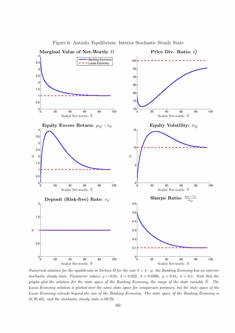
Figure 6: Autarky Equilibrium: Interior Stochastic Steady State
0 20 40 60 80 1000
0.5
1
1.5
2
2.5
3
3.5
4Marginal Value of Net-Worth: Ω
Scaled Net-worth: N
Banking EconomyLucas Economy
0 20 40 60 80 10070
75
80
85
90
95
100
Price Div. Ratio: Q
Scaled Net-worth: N
0 20 40 60 80 1000
0.5
1
1.5
2
2.5
3
3.5
4Equity Excess Return: µQ − rd
%
Scaled Net-worth: N0 20 40 60 80 100
0
5
10
15Equity Volatility: σQ
%
Scaled Net-worth: N
0 20 40 60 80 1000
0.5
1
1.5
2Deposit (Risk-free) Rate: rd
%
Scaled Net-worth: N0 20 40 60 80 100
0
0.1
0.2
0.3
0.4
0.5
0.6Sharpe Ratio: µQ−rd
σQ
Scaled Net-worth: N
Numerical solution for the equilibrium in Section II for the case δ < λ−ρ: the Banking Economy has an interior
stochastic steady state. Parameter values: ρ = 0.01, δ = 0.022, λ = 0.0398, µ = 0.01, σ = 0.1. Note that the
graphs plot the solution for the state space of the Banking Economy, the range of the state variable N . The
Lucas Economy solution is plotted over the same state space for comparison purposes, but the state space of the
Lucas Economy extends beyond the one of the Banking Economy. The state space of the Banking Economy is
(0, 95.43), and the stochastic steady state is 69.76.
60
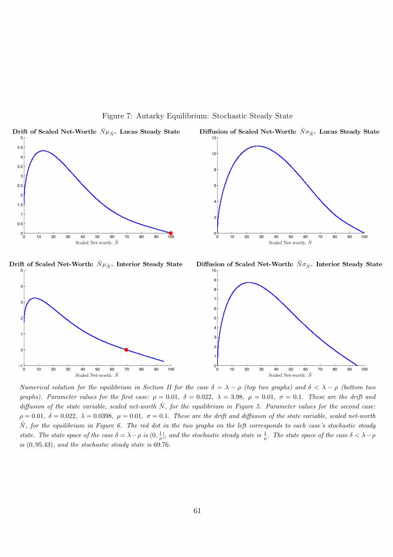
Figure 7: Autarky Equilibrium: Stochastic Steady State
0 10 20 30 40 50 60 70 80 90 1000
2
4
6
8
10
12Diffusion of Scaled Net-Worth: NσN . Lucas Steady State
Scaled Net-worth: N0 10 20 30 40 50 60 70 80 90 1000
0.5
1
1.5
2
2.5
3
3.5
4
4.5
5Drift of Scaled Net-Worth: NµN . Lucas Steady State
Scaled Net-worth: N
0 10 20 30 40 50 60 70 80 90 1000
1
2
3
4
5
6
7
8
9
10Diffusion of Scaled Net-Worth: NσN . Interior Steady State
Scaled Net-worth: N0 10 20 30 40 50 60 70 80 90 100
−1
0
1
2
3
4
5Drift of Scaled Net-Worth: NµN . Interior Steady State
Scaled Net-worth: N
Numerical solution for the equilibrium in Section II for the case δ = λ − ρ (top two graphs) and δ < λ − ρ (bottom two
graphs). Parameter values for the first case: ρ = 0.01, δ = 0.022, λ = 3.98, µ = 0.01, σ = 0.1. These are the drift and
diffusion of the state variable, scaled net-worth N , for the equilibrium in Figure 5. Parameter values for the second case:
ρ = 0.01, δ = 0.022, λ = 0.0398, µ = 0.01, σ = 0.1. These are the drift and diffusion of the state variable, scaled net-worth
N , for the equilibrium in Figure 6. The red dot in the two graphs on the left corresponds to each case’s stochastic steady
state. The state space of the case δ = λ−ρ is (0, 1ρ ], and the stochastic steady state is 1
ρ . The state space of the case δ < λ−ρ
is (0, 95.43), and the stochastic steady state is 69.76.
61

Figure 8: Autarky Equilibrium: Stationary Distribution
0 10 20 30 40 50 60 70 80 900
1
2
3
4
5
6
7
8
9
10
11
Freq
uenc
y %
Scaled Net-worth: NPlot of the limiting stationary distribution of the state variable, scaled net-worth N , for the equilibrium in
Section II for the case δ < λ− ρ. Parameter values: ρ = 0.01, δ = 0.022, λ = 0.0398, µ = 0.01, σ = 0.1. This
is the stationary distribution for the equilibrium in Figure 6. The state space is (0, 95.43), and the stochastic
steady state is 69.76. The approximation to the stationary distribution is obtained by simulating 5,000 paths for
100 years at daily frequency (36,500 periods) for the process N .
62
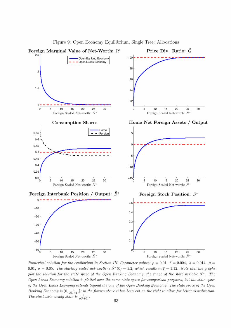
Figure 9: Open Economy Equilibrium, Single Tree: Allocations
0 5 10 15 20 25 301
1.5
2
2.5Foreign Marginal Value of Net-Worth: Ω∗
Foreign Scaled Net-worth: N∗
Open Banking EconomyOpen Lucas Economy
0 5 10 15 20 25 30
92
94
96
98
100
Price Div. Ratio: Q
Foreign Scaled Net-worth: N∗
0 5 10 15 20 25 300.3
0.35
0.4
0.45
0.5
0.55
0.6
0.65
Consumption Shares
Foreign Scaled Net-worth: N∗
HomeForeign
0 5 10 15 20 25 30−15
−10
−5
0
5
Home Net Foreign Assets / Output
Foreign Scaled Net-worth: N∗
0 5 10 15 20 25 30−60
−50
−40
−30
−20
−10
0
Foreign Interbank Position / Output: B∗
Foreign Scaled Net-worth: N∗0 5 10 15 20 25 30
0
0.1
0.2
0.3
0.4
0.5
Foreign Stock Position: S∗
Foreign Scaled Net-worth: N∗
Numerical solution for the equilibrium in Section III. Parameter values: ρ = 0.01, δ = 0.004, λ = 0.014, µ =
0.01, σ = 0.05. The starting scaled net-worth is N∗(0) = 5.2, which results in ξ = 1.12. Note that the graphs
plot the solution for the state space of the Open Banking Economy, the range of the state variable N∗. The
Open Lucas Economy solution is plotted over the same state space for comparison purposes, but the state space
of the Open Lucas Economy extends beyond the one of the Open Banking Economy. The state space of the Open
Banking Economy is (0, 1ρ(1+ξ) ]; in the figures above it has been cut on the right to allow for better visualization.
The stochastic steady state is 1ρ(1+ξ) .
63

Figure 10: Open Economy Equilibrium, Single Tree: Asset Prices
0 5 10 15 20 25 30
0.5
1
1.5
2
2.5Equity Excess Return: µQ − rb
%
Foreign Scaled Net-worth: N∗
Open Banking EconomyOpen Lucas Economy
0 5 10 15 20 25 304.5
5
5.5
6
6.5
7
7.5
8
8.5
9
9.5
10Equity Volatility: σQ
%
Foreign Scaled Net-worth: N∗
0 5 10 15 20 25 300
0.2
0.4
0.6
0.8
1
1.2
1.4
1.6
1.8
2Interbank (Risk-free) Rate: rb
%
Foreign Scaled Net-worth: N∗0 5 10 15 20 25 30
0
0.05
0.1
0.15
0.2
0.25
0.3Sharpe Ratio: µQ−rb
σQ
Foreign Scaled Net-worth: N∗
Numerical solution for the equilibrium in Section III. Parameter values: ρ = 0.01, δ = 0.004, λ = 0.014, µ =
0.01, σ = 0.05. The starting scaled net-worth is N∗(0) = 5.2, which results in ξ = 1.12. Note that the graphs
plot the solution for the state space of the Open Banking Economy, the range of the state variable N∗. The
Open Lucas Economy solution is plotted over the same state space for comparison purposes, but the state space
of the Open Lucas Economy extends beyond the one of the Open Banking Economy. The state space of the Open
Banking Economy is (0, 1ρ(1+ξ) ]; in the figures above it has been cut on the right to allow for better visualization.
The stochastic steady state is 1ρ(1+ξ) .
64
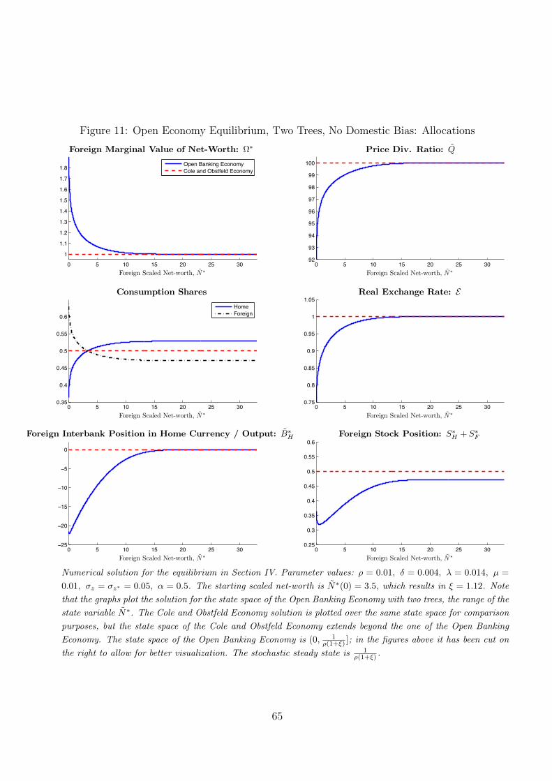
Figure 11: Open Economy Equilibrium, Two Trees, No Domestic Bias: Allocations
0 5 10 15 20 25 301
1.1
1.2
1.3
1.4
1.5
1.6
1.7
1.8
Foreign Marginal Value of Net-Worth: Ω∗
Foreign Scaled Net-worth, N∗
Open Banking EconomyCole and Obstfeld Economy
0 5 10 15 20 25 3092
93
94
95
96
97
98
99
100
Price Div. Ratio: Q
Foreign Scaled Net-worth, N∗
0 5 10 15 20 25 300.35
0.4
0.45
0.5
0.55
0.6
Consumption Shares
Foreign Scaled Net-worth, N∗
HomeForeign
0 5 10 15 20 25 300.75
0.8
0.85
0.9
0.95
1
1.05Real Exchange Rate: E
Foreign Scaled Net-worth, N∗
0 5 10 15 20 25 30−25
−20
−15
−10
−5
0
Foreign Interbank Position in Home Currency / Output: B∗H
Foreign Scaled Net-worth, N∗0 5 10 15 20 25 30
0.25
0.3
0.35
0.4
0.45
0.5
0.55
0.6Foreign Stock Position: S∗
H + S∗F
Foreign Scaled Net-worth, N∗
Numerical solution for the equilibrium in Section IV. Parameter values: ρ = 0.01, δ = 0.004, λ = 0.014, µ =
0.01, σz = σz∗ = 0.05, α = 0.5. The starting scaled net-worth is N∗(0) = 3.5, which results in ξ = 1.12. Note
that the graphs plot the solution for the state space of the Open Banking Economy with two trees, the range of the
state variable N∗. The Cole and Obstfeld Economy solution is plotted over the same state space for comparison
purposes, but the state space of the Cole and Obstfeld Economy extends beyond the one of the Open Banking
Economy. The state space of the Open Banking Economy is (0, 1ρ(1+ξ) ]; in the figures above it has been cut on
the right to allow for better visualization. The stochastic steady state is 1ρ(1+ξ) .
65
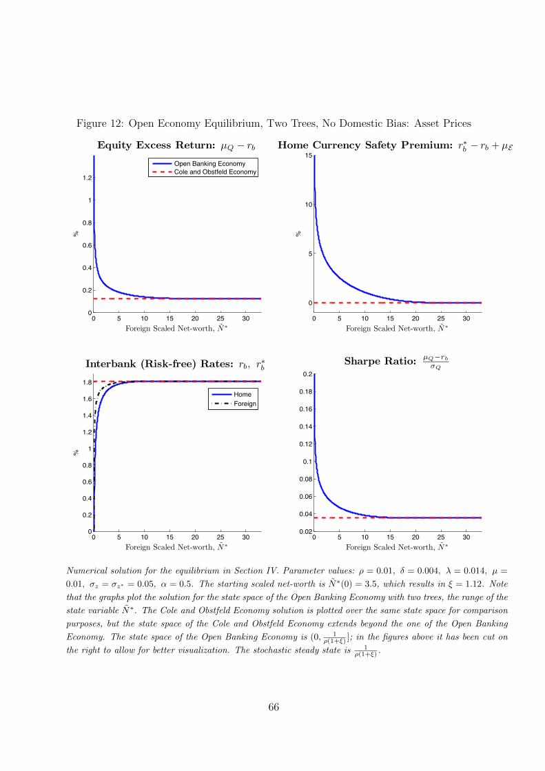
Figure 12: Open Economy Equilibrium, Two Trees, No Domestic Bias: Asset Prices
0 5 10 15 20 25 300
0.2
0.4
0.6
0.8
1
1.2
Equity Excess Return: µQ − rb
%
Foreign Scaled Net-worth, N∗
Open Banking EconomyCole and Obstfeld Economy
0 5 10 15 20 25 30
0
5
10
15Home Currency Safety Premium: r∗b − rb + µE
%
Foreign Scaled Net-worth, N∗
0 5 10 15 20 25 300
0.2
0.4
0.6
0.8
1
1.2
1.4
1.6
1.8
Interbank (Risk-free) Rates: rb, r∗b
%
Foreign Scaled Net-worth, N∗
HomeForeign
0 5 10 15 20 25 300.02
0.04
0.06
0.08
0.1
0.12
0.14
0.16
0.18
0.2Sharpe Ratio: µQ−rb
σQ
Foreign Scaled Net-worth, N∗
Numerical solution for the equilibrium in Section IV. Parameter values: ρ = 0.01, δ = 0.004, λ = 0.014, µ =
0.01, σz = σz∗ = 0.05, α = 0.5. The starting scaled net-worth is N∗(0) = 3.5, which results in ξ = 1.12. Note
that the graphs plot the solution for the state space of the Open Banking Economy with two trees, the range of the
state variable N∗. The Cole and Obstfeld Economy solution is plotted over the same state space for comparison
purposes, but the state space of the Cole and Obstfeld Economy extends beyond the one of the Open Banking
Economy. The state space of the Open Banking Economy is (0, 1ρ(1+ξ) ]; in the figures above it has been cut on
the right to allow for better visualization. The stochastic steady state is 1ρ(1+ξ) .
66