Embed Size (px)
Citation preview

1
No. 09‐13
Financial Leverage, Corporate Investment,
and Stock Returns
Ali K. Ozdagli
Abstract:
This paper presents a dynamic model of the firm with risk‐free debt contracts, investment
irreversibility, and debt restructuring costs. The model fits several stylized facts of corporate
finance and asset pricing: First, book leverage is constant across different book‐to‐market
portfolios, whereas market leverage differs significantly. Second, changes in market leverage
are mainly caused by changes in stock prices rather than by changes in debt. Third, when the
model is calibrated to fit the cross‐sectional distribution of book‐to‐market ratios, it explains
the return differences across different firms. The model also shows that investment
irreversibility alone cannot generate the cross‐sectional patterns observed in stock returns and
that leverage is the main source of the value premium.
JEL Classifications: G1, G3
Ali Ozdagli is an economist in the research department of the Federal Reserve Bank of Boston. His e‐mail address is
This paper, which may be revised, is available on the web site of the Federal Reserve Bank of Boston at
http://www.bos.frb.org/economic/wp/index.htm.
This paper is a modified and improved version of my Ph.D. thesis with the same title. I am grateful to Fernando
Alvarez, Lars Hansen, Anil Kashyap, and Robert Lucas for their support. I also thank Federico Diez, Sergey Kulaev,
Christina Wang, and the seminar participants at the University of Chicago, in particular, Gene Fama and Jarda
Borovicka, for helpful comments, and Sarojini Rao for excellent research assistance. The usual disclaimer applies.
The views and opinions expressed in this paper are those of the author and do not necessarily represent the views
of the Federal Reserve Bank of Boston or the Federal Reserve System.
This version: November 13, 2009

1 Introduction
Firms with a high ratio of book value of equity to market value of equity (value �rms) earnhigher expected stock returns than �rms that have low book-to-market equity ratio (growth�rms). However, as Grinblatt and Titman (2001) point out, conventional wisdom tells usthat growth options should be riskier than assets-in-place:
Consider Wal-Mart, for example. The value of this �rm's assets can be re-garded as the value of the existing Wal-Mart outlets in addition to the valueof any outlets that Wal-Mart may open in the future. The option to open newstores is known as a growth option. Because growth options tend to be mostvaluable in good times and have implicit leverage they contain a great deal ofsystematic risk.
Therefore, as Zhang (2005) stresses, conventional wisdom suggests that growth �rms,which derive their value from growth options, should have higher expected stock returnsthan value �rms, which derive their value from assets-in-place.To add insult to injury, Fama and French (1992) show that portfolios of stocks with
different book-to-market ratios have similar riskiness as measured by the standard CapitalAsset Pricing Model (CAPM) of Sharpe (1964), Lintner (1965), and Black (1972). Thisphenomenon, known as the �value premium puzzle,� helped the Fama and French modelreplace the CAPM as the benchmark in the asset pricing literature.This paper explains the differences between the stock returns of value and growth �rms.
For this purpose, I extend the investment irreversibility model of Abel and Eberly (1996)by incorporating investors' risk preferences, risk-free debt contracts, and debt adjustmentcosts. Using this framework, I show that �nancial leverage can explain the major shareof the value premium, while investment irreversibility alone generates a growth premiumrather than a value premium. However, investment irreversibility is still an important in-gredient that improves the model's �t with the data, by generating a wide range of book-to-market values.The �nancing decisions in this model are similar, but not identical, to those of Fischer,
Heinkel, and Zechner (1989) and Gomes and Schmid (2009). Those papers add debt re-structuring costs to the standard tradeoff theory of capital structure whereby a �rm choosesits �nancing policy by balancing the costs of bankruptcy against the bene�ts of debt, suchas tax shields due to interest payments. My paper also assumes that �rms bene�t from thetax shield of debt as in the tradeoff theory and that they face additional costs at the time ofdebt restructuring. However, in this paper, debt has two properties distinct from its proper-
2

ties in previous papers: it is risk-free and endogenously limited by the lenders to a certainfraction of capital.The choice of risk-free debt serves simplicity, conformity to data, and consistency:
First, it simpli�es the analysis of the model by removing the need to keep track of themarket value of leverage separately. Second, it �ts the facts, presented in Fama and French(1993), that the book-to-market factor does not affect bond returns and that �average excessbond returns are close to zero� so that �the hypothesis that all the corporate and governmentbond portfolios have the same long-term expected returns cannot be rejected�(6). Finally,because we do not observe the market value of debt, many studies that relate risky debtto returns use book value of leverage as a proxy for market value of leverage. However,this contradicts the assumption of risky debt, and so the approach defeats the purpose.Therefore, for the sake of consistency, I stick to risk-free debt.The debt limit of a �rm is determined endogenously in the following way: Since interest
payments are tax deductible, the �rm prefers debt �nancing to equity �nancing and wouldrather have an in�nite amount of debt. However, this leads to negative equity value insome states, so that the �rm would rather go bankrupt than pay its debt. Therefore, fordebt to remain risk-free, lenders will limit the amount of debt. They can accomplish thisby accepting the resale value of capital as collateral and ensuring that this value is notlower than the amount of debt, so that they can recover their money in case of bankruptcy.1
Alternatively, lenders may limit the amount of debt in order to ensure that the market valueof equity is always non-negative and that bankruptcy is suboptimal for the �rm. I showthat the market value of equity is strictly positive when the debt capacity equals the resalevalue of capital. Therefore, the market value of equity would still be non-negative if thelenders would lend the �rm more than the resale value of its capital. Thus, the latter policyprovides the �rm with a higher debt capacity and the �rm prefers this latter debt policy,while the lenders are indifferent.An important property of the model is that the �rm's book leverage, that is, the fraction
of total capital supplied by lenders, is not state-dependent. The book leverage is determinedin a manner that ensures that the �rm value is non-negative even in the worst-case scenario,to avoid bankruptcy. I show that this worst-case scenario is independent of the state vari-ables and hence a revision of the debt agreement at a later date would lead to the samelevel of leverage. As a result, it is not optimal for a �rm to change its book leverage onceit is set, and the book leverage remains the same across �rms with different ratios of book-to-market equity, whereas market leverage differs signi�cantly. Figure 1 plots averages of
1This is a common assumption in the papers that model risk-free debt. A recent example is Livdan,Sapriza, and Zhang (2009).
3

Figure 1: Book leverage and market leverage across different book-to-market value portfo-lios created using the method in Fama and French (1992). The numbers on the horizontalaxis give the average book-to-market equity value in each portfolio. The numbers on thevertical axis give the average market and book leverage in each portfolio. Source: TheCenter for Research in Security Prices, CRSP-COMPUSTAT merged database, and au-thor's calculations.
book and market leverage within different book-to-market portfolios and provides supportfor this argument.2 Moreover, because the level of debt is constant in the inaction region(when the �rm does not invest) the �rm's market debt-to-equity ratio varies closely with�uctuations in its own stock price. This implication of the model is in line with the resultsof Welch (2004), who �nds that U.S. corporations do little to counteract the in�uence ofstock price changes on their capital structures.My analysis shows that the investment irreversibility alone causes a growth premium
rather than a value premium. The �rm's investment opportunity is a call option, becausethe �rm has the right but not the obligation, to buy a unit of capital at a predeterminedprice. As we know from the �nancial options literature, when the price of the underlyingsecurity rises and falls, the price of the call option rises and falls at a greater rate. Thissuggests that the value of a growth option, that is, the call option to invest, should be moreresponsive to economic shocks than the assets-in-place. Therefore, growth options increasethe riskiness of the �rm. Similarly, the disinvestment opportunity is a put option, because
2This further supports the choice of risk-free debt over risky debt. In a tradeoff model, it is optimalfor more productive �rms to have greater book leverage, since debt is less costly for them, which wouldcontradict the data.
4

the �rm has the right, but not the obligation, to sell a unit of capital at a predeterminedprice. The value of this put option is negatively related to the value of the underlyingasset, because the gain from exercising it is higher for less productive �rms. Therefore,the disinvestment option provides the value �rms that have low productivity with insuranceagainst downside risk and hence reduces their riskiness. This proposition is contrary to thewisdom of recent literature, for example, Zhang (2005) and Cooper (2006), which presentsinvestment irreversibility as the source of the value premium.In my model, �nancial leverage affects stock returns directly, through its effect on eq-
uity risk à la Modigliani and Miller (1958), and indirectly, through its effect on businessrisk, by in�uencing investment decisions. I �nd that these two channels have opposingeffects on the relationship between book-to-market ratios and stock returns. However, theModigliani-Miller effect strongly dominates the investment channel and explains the majorshare of the value premium.The Modigliani-Miller (1958) effect of debt comes from the fact that the book-to-
market ratio and market leverage are closely related when book leverage is constant aswe observe within the context of this model. In particular, if we let BE;ME, BL, andML be book value of equity, market value of equity, book leverage, and market leverage,respectively, and use the fact that the market value of debt is equal to the book value of debtwhen debt is risk-free, we have
BE
ME=
ML
1�ML1�BLBL
:
Because book value is constant across value and growth �rms, this equation implies thatvalue �rms have higher market leverage than growth �rms. Therefore, they have greaterequity risk according to the Modigliani and Miller theorem.Financial leverage also affects investment and hence the business risk, because it in-
�uences the effective degree of investment irreversibility faced by the owners of the �rm.When investment can be �nanced with leverage, the effective price of capital is reducedby the tax savings associated with debt �nancing at the time of investment. On the otherhand, at the time of disinvestment, the �rm has to pay back its debt, in line with the debtagreement and therefore has to give up the tax savings associated with the debt �nancing ofthat particular investment. Because the purchase price is greater than the resale price andboth should be adjusted by the same value of tax savings, their ratio increases as a resultof debt �nancing. This increases the effective irreversibility perceived by the owners of the�rm. Since irreversibility reduces the value premium, so, too, does the investment channelof leverage.
5

This paper is closely related to the growing literature that tries to link corporate deci-sions to asset returns. In addition to Zhang (2005) and Cooper (2006) discussed above,Carlson, Fisher, and Giammarino (2004) link the value premium to operating leverage.Livdan, Sapriza, and Zhang (2009) look at the effect of exogenous risk-free debt capacityon stock returns, and Gomes and Schmid (2009) link leverage and growth options to assetreturns. The paper contributes to this literature in many ways. First, the closed-form solu-tion of the model identi�es explicitly how investment irreversibility, �nancial leverage, andtheir interaction affect the cross-section of stock returns. Second, the debt capacity of the�rm is endogenously determined. Third, the paper does not need to rely on a high degreeof irreversibility in order to generate a sizable variation in stock returns, because of theinteraction of �nancial leverage and irreversibility.3 Fourth, the paper calibrates the modelusing maximum likelihood to capture the distribution of book-to-market values instead ofplugging in parameter values in an ad hoc manner and the calibrated model captures thedistribution of market leverage reasonably well.4 Finally, the paper shows that �nancialleverage can explain the value premium.The next section presents the problem of the �rm in a continuous time setting. The
third section then discusses the optimal investment policy and the market value of equity.The fourth section presents optimal �nancing policy and its relationship with investment.The �fth section links stock returns with investment irreversibility and �nancial leverage.The two sections thereafter present the calibration of the model and the comparison ofsimulation results with the data. The section thereafter provides an extension of the model,introducing the time varying-price of capital to account for the failure of the CAPM, andthe last section concludes.
2 The Model
My model extends the investment irreversibility model of Abel and Eberly (1996) withcorporate taxes, debt, and a stochastic discount factor to capture investors' risk preference.While debt capacity and investment and �nancing decisions are endogenous, investors'
3The degree of irreversibility assumed by the cited papers implies that the net value generated by disin-vestment is non-positive after adjustment costs are included. However, Hall (2004) estimates the adjustmentcost parameter for capital in a quadratic adjustment cost model without debt and �nds that adjustment costsare relatively small and are not an important part of the explanation of the large movements in companyvalues.
4To the best of my knowledge, no other paper in the literature makes an effort to match the distribution ofbook-to-market values and leverage, although this distribution is important in generating the cross-sectionaldistribution of returns. The implications of omitting this fact are crucial and are discussed in the Calibrationsection.
6
preferences are captured by an exogenous discount factor, as in Zhang (2005), Cooper(2006), and Carlson, Fisher, and Giammarino (2004), among others.The �rms choose their investment and �nancing policy in order to maximize the market
value of equity. Investment is subject to partial irreversibility, that is, the purchase price ofone unit of capital is 1 and the resale price is � < 1. Each �rm produces output at time tusing capital,Kt, and takes the level of productivity, Xt, and the stochastic discount factorof investors, St, as exogenously given. BothXt and St follow geometric Brownian motions
dXtXt
= �Xdt+ �AdwA + �idwi = �Xdt+ �dw
dStSt
= �rdt� �SdwA;
where Et[�dSt=St] = rdt is the interest rate and �S is the price of risk.5 The Brownianincrements dwA and dwi represent systematic and idiosyncratic shocks and are independentof each other. They can be aggregated using � =
p�2i + �
2A and dw = (�i=�) dwi +
(�A=�) dwA. Moreover, if we let Ut and Lt denote total capital purchases and total capitalsales, respectively, up to time t, we can write the net change in the stock of capital as
dKt = dUt � dLt;
where dUt � 0 and dLt � 0.The net income of the �rm is given by the operating cash �ows net of the cost of
maintenance and cash �ows to debtholders plus tax shields from depreciation and interestpayments:
�� (Kt; Xt; bt) = (1� �)�
h
1� X t K
1� t � �Kt � rbtKt
�;
where � is the tax on corporate income, h > 0 is the productivity multiplier, and 0 < < 1is the returns-to-scale parameter of the production function.6 On the cash out�ow side, � isthe maintenance cost per unit of capital, r is the risk-free rate on debt, and bt is the fractionof the capital provided by the lenders, or book leverage.I model �nancial leverage as risk-free debt extended through a credit line where the5This stochastic discount factor can be derived as the result of time-separable constant relative risk aver-
sion utility with a constant discount rate, where consumption follows a geometric Brownian motion, or linearutility with a time-varying discount rate.
6This functional form nests a Cobb-Douglas production function with an isoelastic demand curve and ageometric Brownian motion technology process in which variable inputs, such as labor, have been optimizedout.
7

debtholders agree to �nance a certain fraction of operating capital. Intuitively, the lenderscan keep the debt risk-free by a collateralized debt agreement and can limit the amount ofdebt by the resale price of capital so that � � b. Alternatively, they can set a limit on debtthat guarantees that the �rm always has non-negative market equity and hence honors itsdebt rather than going bankrupt. The �rm has the option to renegotiate this fraction later,but debt restructuring requires that the existing debt be retired altogether and that the newdebt be issued at a cost proportional to the amount of new debt, c, as in Fisher, Heinkel,and Zechner (1989).As a result of this credit line, the �rm will invest when the marginal value of capital
to equity holders is 1 � b, as this is the fraction of new investment that should be �nancedwith equity. Moreover, the �rm will disinvest when the marginal value of capital is � � b,because the �rm gets � for each unit of capital sold but has to give back b to debtholdersin order to keep the book leverage constant, in accord with the debt agreement. In thefollowing analysis, XU (K; b) denotes the investment boundary along which the marginalvalue of capital is 1� b, while XL (K; b) denotes the disinvestment boundary along whichthe marginal value of capital is � � b. These two boundaries enclose the inaction regionwhere the marginal value of capital is between 1� b and � � b and net investment is zero.This investment policy will be discussed in more detail in the next section.7
The following proposition establishes that the �rm will never go bankrupt under a col-lateralized debt agreement.
Proposition 1 The market value of equity is strictly positive if debt is limited by the resaleprice of capital and the marginal value of capital is right-continuous at the investmentboundary.
Proof. We have � � b if debt is limited by the resale price of capital. The market valueof equity is bounded by (� � b)K � 0, because this is what the shareholders will getafter paying the lenders if they decide to dissolve the �rm. Let J (X;K; b) be the marketvalue of equity and KU (X; b) be the inverse of the investment boundary XU (K; b) withrespect to capital. Then J (X;KU (X; b) ; b) > (� � b)K must hold, since otherwise the�rm would dissolve immediately, leaving the shareholders with capital (� � b)K in returnto their investment (1� b)K. Therefore, J (X;KU (X; b) ; b) > 0. Finally, we can writethe market value of equity as
J (X;K; b) = J (X;KU (X; b) ; b) +
Z K
KU (X;b)
JK (X; k; b) dk;
7I assume that the accounting salvage value of the capital is the same as the actual salvage value, for thesake of simplicity so that the �rm does not pay any taxes on resale price of capital.
8

where 1 � b � JK (X;K; b) � (� � b) � 0, because the marginal value of capital isbounded due to investment and disinvestment options. Moreover, JK (X;KU (X; b) ; b) =
1 � b > 0 because b � � < 1. Because the marginal value of capital is right-continuous,this implies that JK (K;X; b) > 0 for values of K arbitrarily close to KU (X; b). We alsohave K � KU (X; b) for any given X and b, because the �rm will invest to prevent thevalue of capital from falling below KU (X; b). Therefore, the integral on the right side ofthis equation should be positive. Since sum of the two positive terms is positive, we haveJ (X;K; b) > (� � b)K � 0, and this completes our proof.This proposition essentially tells us that even if the �rm had the option to go bankrupt, it
would never exercise this option when debt is limited by the resale price of capital, becausethe disinvestment boundary would be hit before bankruptcy becomes optimal.8 It followsimmediately that the debt agreement with a no-bankruptcy condition is less restrictive. Inparticular, it should provide a greater debt limit because the market value of equity wouldstill be non-negative if the lenders lent the �rm more than the resale value of its capital.Since bankruptcy is suboptimal under both lending policies, I omit bankruptcy in the restof the paper.The �rm maximizes shareholder value by choosing its investment and �nancing plans:
J (Kt; Xt; bt) = maxfdUt+s;dLt+s;dbt+sg
Z 1
0
St+sSt
[��t+sds� (1� bt+s)dUt+s + (� � bt+s) dLt+s]
+1X
s2fs:dbt+s 6=0g
St+sSt
[dbt+s � c(bt+s + dbt+s)]Kt+s;
where the term dbt+s is the change in book leverage after debt adjustment, andR10dUt+s
andR10dLt+s are Stieltjes integrals. Note that the stochastic discount factor does not ap-
pear as a state variable in the value function J because St+s=St is log-normally distributedwith parameters rt and �2St and this distribution does not depend on any state variable.The debt limit imposed by the lenders adds an additional constraint to the problem. If
debt is limited by the resale value of capital, then this constraint is simply bt+s � �.9 If, onthe other hand, debt is limited by the no-bankruptcy condition then we have
0 � J (Kt+s; Xt+s; bt+s) for all Kt+s; Xt+s; bt+s:
8Note that, in order to minimize the burden on the reader, the proof does not depend on any functionalassumptions regarding the market value of equity and does not require modeling the bankruptcy option ex-plicitly. However, the calculations for the �rm with the bankruptcy option are available upon request.
9Although I have shown that the debt policy with the no-bankruptcy condition provides a greater debtcapacity than the collateralized debt policy, I still cannot rule out the latter until I show that debt �nancing ispreferred to equity �nancing, which I show in the next section.
9

Because of investment and debt adjustment costs, it is not optimal for the �rm to adjustcapital and debt frequently. The Hamilton-Jacobi-Bellman equation (HJB) in the inactionregion where the �rm does not make any adjustments is given by
rJ (K;X; b) = �� (K;X; b) + �XJX (K;X; b) +1
2�2X2JXX (K;X; b) ; (1)
where � = �X � �S�A is the risk-adjusted drift of the productivity process.10 When wedivide both sides of this equation by the market value of equity, J , this equation tells usthat the required rate of return from buying the �rm should be equal to the dividend yield(the �rst term) plus capital appreciation (the second and third terms).The boundary conditions11 at the investment boundary, XU (K; b), are
JK (K;XU (K; b) ; b) = 1� bJKK (K;XU (K; b) ; b) = 0
JKX (K;XU (K; b) ; b) = 0
JKb (K;XU (K; b) ; b) = �1;
while the boundary conditions at the disinvestment boundary, XL (K; b), are given by
JK (K;XL (K; b) ; b) = � � bJKK (K;XL (K; b) ; b) = 0
JKX (K;XL (K; b) ; b) = 0
JKb (K;XL (K; b) ; b) = �1:
Finally, if we denote the book leverage after adjustment as b0, the boundary conditions atthe debt adjustment boundary are given by
J (K;XB (K; b) ; b) = J (K;XB (K; b) ; b0) + (b0 � b)K � cb0K
JK (K;XB (K; b) ; b)� cb = JK (K;XB (K; b) ; b0) + (b0 � b)� cb0
JX (K;XB (K; b) ; b) = JX (K;XB (K; b) ; b0)
Jb (K;XB (K; b) ; b) = �K�(1� c)K � Jb (K;XB (K; b) ; b
0) :
10This is essentially the same as substituting the stochastic discount factor with the risk-free rate and takingexpectations under the risk-neutral measure.11These conditions are known as value-matching and smooth pasting conditions that guarantee the con-
tinuity and optimality of the value function. Dixit (1993) is a good introduction for the derivation of theseconditions.
10
The last of these conditions is the �rst order condition with respect to after-adjustmentleverage, b0 under debt constraint. Hence it holds as an equality if the new book leveragesatis�es b0 < � or J (K;X; b0) > 0, depending on the constraint imposed by the lender. Themarket value of equity, J (X;K; b), should be homogeneous of degree one in K and X ,because the cash�ows and the adjustment costs on debt and investment are homogeneousin K and X .12
3 Optimal Investment Policy and the Valuation of Equity
Since equation (1) holds identically in K, we can take the derivative of both sides withrespect to K to get
rJK (K;X; b) = ��K (K;X; b) + �XJKX (K;X; b) +1
2�2X2JKXX (K;X; b) :
Because all terms in the �rm's problem are homogeneous of degree one in X and K, thevalue of the �rm should also be homogeneous of degree one in X and K. As a result, themarginal value of capital should be homogeneous of degree zero in X and K. Therefore,we can de�ne y � X=K and q (y; b) � JK (K;X; b) to express the last equation as
rq (y; b) = �hy � �m+ �yqy (y; b) +1
2�2y2qyy (y; b) ; (2)
where �h = (1� �)h and �m (b) = (1� �) (� + rb) is the marginal cost of maintenance and�nancing. Then, the boundary conditions at the upper and lower investment bounds aregiven by the following equations.13
q (yL (b) ; b) = � � b and qy (yL (b) ; b) = 0 (3)
q (yU (b) ; b) = 1� b and qy (yU (b) ; b) = 0: (4)
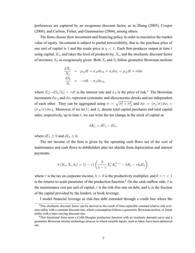
This reduces the original HJB equation to an ordinary differential equation; solving this in-volves �nding two constants of integration and the boundary values for y. Figure 2 displaysthe projection of the investment and inaction regions implied by the boundary conditions12This argument is similar to the one in Abel and Eberly (1996) and Cooper (2006). To justify this homo-
geneity property and hence that X=K is a suf�cient statistic to describe the solution of the model, the readercan directly substitute in V (y; b) � V (X=K; b) = J (X;K; b) =K and see that both the HJB equation andthe boundary conditions can be expressed in terms of V (y; b) and its derivatives.13We can see that the additional smooth pasting conditions for b, that is, qb (yL (b) ; b) = qb (yL (b) ; b) =
�1 are automatically satis�ed once we take the derivative of the value-matching equations and apply thesmooth pasting conditions for y. Therefore, we omit these conditions for the rest of the analysis.
11

X
K
Slope = yU(b)
Slope = yL(b)
disinvestmentregion
investmentregion
inaction region
bqb −<<− 1η
bq −=1
bq −=η
Figure 2: Projection of investment and inaction regions on the K-X plane. The line withslope yU (b) gives the investment boundary, while the line with slope yL (b) gives the dis-investment boundary. These two boundaries enclose the inaction region for investment.Source: Author's calculations.
on the (K;X) plane.The appendix shows that solving these equations and integrating the marginal value of
capital leads to
J (K;X; b) = �HX K1� + �DP (b)X�PK1��P + �DN (b)X
�NK1��N � �m (b)
rK; (5)
where �P > 1 > > 0 > �N , �DP (b), and �DN (b) are functions of book leverage that takeonly positive values.14 The four terms are the value of assets in place (before costs), growthoptions, disinvestment options, and the present value of operating and �nancing costs.
4 Financial Leverage and Investment
We now turn our attention to optimal �nancing policy and its relationship with investment.The following proposition shows that the tax advantage of leverage makes the �rm chooseits investment policy as if it faced greater irreversibility. Then I will show that the optimal14Note that the derivation of the market value of equity does not make use of the boundary conditions for
debt restructuring.
12

�nancing policy for the �rm is to exhaust its debt capacity. Therefore, the �rm prefers theno-bankruptcy condition because it provides greater debt capacity. Finally, I show that thedebt capacity under the no-bankruptcy condition is independent of state variables.
Proposition 2 When interest payments are tax deductible, the gap between the investmentboundary and the disinvestment boundary as measured byG (b) � yU (b) =yL (b) increaseswith book leverage b.
Proof. See appendixIntuitively, the gap between the investment and disinvestment boundaries increases as
the ratio of the purchase to the resale price increases, because it is this discrepancy betweenprices that creates investment irreversibility. Then, we should answer why the purchaseprice increases relative to the resale price. When investment is �nanced with leverage, theshareholders care not only about the actual price of capital but also about the �nancingcosts. At the time of investment, the net purchase price of capital from the shareholders'perspective is the actual price net of any tax savings due to debt �nancing. At the timeof disinvestment, the net resale price of capital is the actual price minus the loss of taxdeductions due to debt repayment. Since the purchase and resale prices of capital increaseby the same amount of tax savings, their ratio should increase. This increases the effectiveirreversibility perceived by the shareholders.The next two propositions show that the optimal behavior for the �rm is to use all of its
debt capacity at once if the cost of issuing debt is suf�ciently small so that the tax savingsdue to interest payments dominate the cost of debt �nancing and never to adjust its bookleverage after that. I assume that the cost of issuing debt is below this limit.
Proposition 3 Let G (b) � yU (b) =yL (b) > 1. Then, there is a critical level for the cost ofissuing debt, given by
c� = �
�1� 1
1� �N
�> 0
below which the �rm strictly prefers debt to equity.
Proof. See appendix
Proposition 4 It is never optimal to readjust debt.
Proof. The appendix shows that Jb (X;K; b) + K � 0. Therefore, the smooth pastingconditions required at the disinvestment boundary are not satis�ed.The following proposition shows that the leverage limit set by the debtholders is the
same for all �rms regardless of their productivity and capital levels.
13

Proposition 5 The debt limit implied by the no-bankruptcy condition is not state-dependent.
Proof. Using equation (5) we can write the no-bankruptcy condition J (K;X; b) � 0 asJ (K;X; b) =K = J (1; y; b) � 0, that is
J (1; y; b) = Hy +DP (b) y�P +DN (b) y
�N � �m
r� 0:
Moreover, J (1; y; b) should be increasing in y because, given capital and leverage, moreproductive �rms should have higher market value, that is, JX (K;X; b) > 0. Therefore,J (K;X; b) � 0 for all (X;K; b) if and only if J (1; yL (b) ; b) � 0. As a result, the debtlimit is given by the equation J (1; yL (b) ; b) = 0, whose solution is independent of statevariables.
This proposition tells us that the book leverage in this model should not be state-dependent because the debt limit is determined by the worst-case scenario, which is alsonot state-dependent due to the homogeneity of the �rm's value. This result is importantfor two reasons: First, it strengthens the result that it is not optimal to adjust debt once itis set because it is costly to adjust and the new limit would be the same as the old one.Second, because the debt limit as a fraction of total capital is the same for all �rms, bookleverage is the same across �rms with different book-to-market ratios. Figure 1 shows thatthis implication of the model �ts the data.
5 Stock Returns
5.1 Investment Irreversibility and Stock Returns
In order to isolate the pure effect of investment irreversibility of stock returns, I focus on a�rm that does not have any operating costs and �nancial leverage. In this case, the marketvalue of �rm's equity is given by
J (K;X) = HX K1� +DPX�PK1��P +DNX
�NK1��N ;
where �P > 1 > > 0 > �N and H ,DP , and DN are positive constants. These threeterms capture market value of the assets-in-place, the growth options, and the disinvestmentoptions, which I denote JAP ; JG, and JD respectively.Using Ito calculus and some algebra we can derive the (conditional) expected excess
14

stock return as
1
dtE (dR)� r =
1
dtE
��dt+ dJ
J
�� r = �S�A
JXX
J
= �S�A
�JAP
J +
JG
J�P +
JD
J�N
�= �S�A (sAP + sG�P + sD�N) :
Therefore, the excess stock return is a value-weighted average of excess returns that comefrom the three sources of value. Since the book-to-market ratio can be expressed asK=J (K;X) =1=J (1; y), the ratio of productivity to capital is a suf�cient statistic that is negatively re-lated to the book-to-market ratio. It is then straightforward to show that the stock returnincreases in y and hence decreases in book-to-market values, producing a growth premiumrather than a value premium.15
The result presented in this section is intuitive, once we realize the similarities of growthand disinvestment options with �nancial options. The �rm's investment opportunity is acall option because the �rm has the right, but not the obligation, to buy a unit of capital ata predetermined price. As we know from the �nancial options literature, as the price of theunderlying security rises and falls, the price of the call option rises and falls at a greater ratethan the underlying security.16 This suggests that the value of the growth option, that is, thecall option to invest, should be more responsive to pro�tability shocks, and hence riskier,than the assets-in-place. This is captured by �P > in this model. As a result, growth�rms, which derive their value mainly from growth options should have higher expectedreturns than value �rms.Similarly, the disinvestment opportunity is a put option, because the �rm has the right,
but not the obligation, to sell a unit of capital at a predetermined price. The value of thisput option is negatively related to the value of the underlying asset, because the gain fromexercising the option, that is, disinvestment, is higher for less productive �rms. Therefore,the disinvestment option provides the value �rms with insurance against downside risk andhence reduces their riskiness. In this model, this is captured via �N < 0.This result is in contrast with the intuition of several recent papers, such as Zhang
(2005) and Cooper (2006), that present investment irreversibility as the source of the valuepremium. These papers argue that investment adjustment costs make it harder for value15Intuitively, the assets-in-place and growth options build a higher fraction of market value for �rms with
a higher productivity-to-capital ratio. This fact, combined with the arithmetic signs of the parameters, leadsto a positive derivative of stock returns with respect to y. The appendix provides the calculus.16The call option is implicitly leveraged: If we denote the underlying security price with S and the strike
price with K, the payoff of the call options is S-K, which has the elasticity d ln(S �K)=d lnS > 1, wherethe strike price,K, is the leverage.
15

�rms to deploy their excess capital when the economy faces bad shocks, whereas growth�rms do not face the same problem, as they do not have too much excess capital. As aresult, assets-in-place should be riskier than growth options and hence value �rms shouldbe riskier than growth �rms. However, these papers include �xed operating costs in thepro�t function of the �rm, which would affect the business risk, possibly creating a valuepremium as Carlson, Fisher, and Giammarino (2004) suggest. Unfortunately, these papersdo not provide an analysis of how much of the difference in returns is accounted for by theirreversibility and operating leverage.17
The following proposition generalizes the argument that growth options are riskier thanassets-in-place, by providing a proof that does not depend on the properties of the ad-justment cost or of the processes for productivity or the stochastic discount factor. Theproposition focuses on total irreversibility of investment because, if the irreversibility werethe main reason for value premium, it should create the greatest value premium if �rmswere not able to disinvest.
Proposition 6 In the absence of leverage and under perfect investment irreversibility, growthoptions are riskier than assets-in-place.
Proof. In case of perfect irreversibility the �rm does not have a disinvestment option.Therefore, the market value of equity consists of value of growth options and assets-in-place only. If we let rAP be the return on assets in place and rG be the return on the growthoption, we can write the expected returns to equity as
rE =JAP (K;X)
J (K;X)rAP +
JG (K;X)
J (K;X)rG;
where
J (K;X) = JAP (K;X) + JG (K;X)
rE =JXJ
����cov�dX; dSS�����
rAP =JAPXJAP
����cov�dX; dSS�����
rG =JGXJG
����cov�dX; dSS����� :
17Zhang (2005) provides (in Table IV) a sensitivity analysis that shows that a 10 percent reduction in �xedcosts reduces the difference between stock returns of the �rms in the highest and lowest book deciles by 1percent. Unfortunately, there is no analysis about how the model performs when the �xed costs are set tozero. However, if we assume that the elasticity of return differences to �xed costs is constant, eliminatingoperating leverage should lead to a 10 percent decrease in the value premium between highest and lowestdeciles and hence nullify the stock return differences.
16

Moreover, given capital, �rms with higher productivity have lower book-to-market values,and hence are growth �rms, for which the growth options constitute a greater share ofmarket value. Therefore, we should have
@JG (K;X) =J (K;X)
@X> 0:
With a little algebra, we can show that
@JG (K;X) =J (K;X)
@X=JG (K;X) =J (K;X)��cov �dX; dS
S
��� (rG � rE) ;
which together with previous inequality implies that rG > rE > rAP . Therefore, growthoptions are risker than assets-in-place.It follows, from this proposition, that growth �rms that derive their value from growth
options should have higher expected returns so that we have a growth premium rather thana value premium under investment irreversibility without leverage.Despite the negative relationship of value premium and investment irreversibility, I keep
irreversibility in my model because it is useful to generate a wide range of book-to-marketvalues, and market leverage, and hence variation in stock returns. In particular, note that inthe absence of irreversibility, the excess returns would be the same for all �rms and equalto �S�A.
5.2 Financial Leverage and Stock Returns
Using Ito calculus and the Hamilton-Jacobi-Bellman equation (1) from the previous sec-tion, we can write the excess stock returns as
dRi�rdt =�� (Ki; Xi) dt+ dJ (Ki; Xi)
J (Ki; Xi)�rdt = �S�A
XiJiX (Ki; Xi)
Ji (Ki; Xi)dt+
XiJiX (Ki; Xi)
Ji (Ki; Xi)�dw;
(6)where �S is the price of risk, �AXiJiX(Ki;Xi)
Jiis the risk exposure, and �dw = �AdwA +
�idwi. The appendix shows that we can rewrite excess stock returns as
1
dtE (dRi)� r =
�1 +
�m (b) =rK
J
�( sAP + �P sG + �NsD)�S�A; (7)
where the �rst factor captures the Modigliani-Miller effect, and the second factor decom-poses the total business risk (as if the �rm were all equity �nanced) into assets-in-place, agrowth option, and a disinvestment option.
17

Financial leverage affects returns in two ways. The �rst effect, the Modigliani-Millerchannel, is obvious in equation (7). Firms with higher market leverage, bK=J , also havehigher book-to-market values, (1� b)K=J , when book leverage, b, is constant. This makesthe equity of �rms with higher book-to-market value riskier.The second effect comes from the interaction of �nancial leverage and investment. We
have seen that �nancial leverage increases the effective degree of irreversibility faced bythe owners of the �rm and that irreversibility causes a growth premium, rather than a valuepremium. Therefore, the effect of leverage on business risk, which is captured by thesecond factor in equation (7), counteracts the Modigliani and Miller effect.The net effect of leverage on stock returns depends on the parameterization of the
model, which we will focus on next.
6 Calibration
Some parameters of the model have direct counterparts in the data. Accordingly, the taxrate is taken to be 35 percent from Taylor (2003). The risk-free rate is taken to be 2 percent,using a time series average of Fama's monthly T-bill returns from the CRSP database from1963 to 2007. The yearly value of �S is set to 0:11 in order to match the average monthlySharpe ratio of the excess market return, using the excess market return series fromKennethFrench's webpage, again from 1963 to 2007. Finally, the book leverage is set equal to0:50.18
The remaining parameters for which we do not have direct observations are estimatedvia maximum likelihood, using the long-run stationary distribution of the book-to-marketvalues from Compustat. I could calibrate all the parameters using a collection of numbersfrom other papers such as Zhang (2005), Cooper (2006), or Gomes and Schmid (2009),or I could estimate the parameters that �t the distribution of returns, as in Carlson, Fisher,and Giammarino (2004). Instead I make use of the distribution of book-to-market values,because explaining the cross-section of returns consists of two important steps: gettingthe relationship between returns and book-to-market values right and getting getting thedistribution of book-to-market values right. If the model fails any of these steps, it cannotproduce the correct distribution of returns. Even worse, a model can claim to explain thecross-section of returns correctly although it fails in both steps. Therefore, starting theanalysis with the distribution of the book-to-market values provides a consistency check.18Because of the interaction between resale price of capital and book leverage, it is enough to preset only
one of these parameters. Since there is no consensus regarding the exact value of the resale price of capital,whereas we actually observe the book values from Compustat, I preset book leverage and estimate the impliedresale value of capital.
18

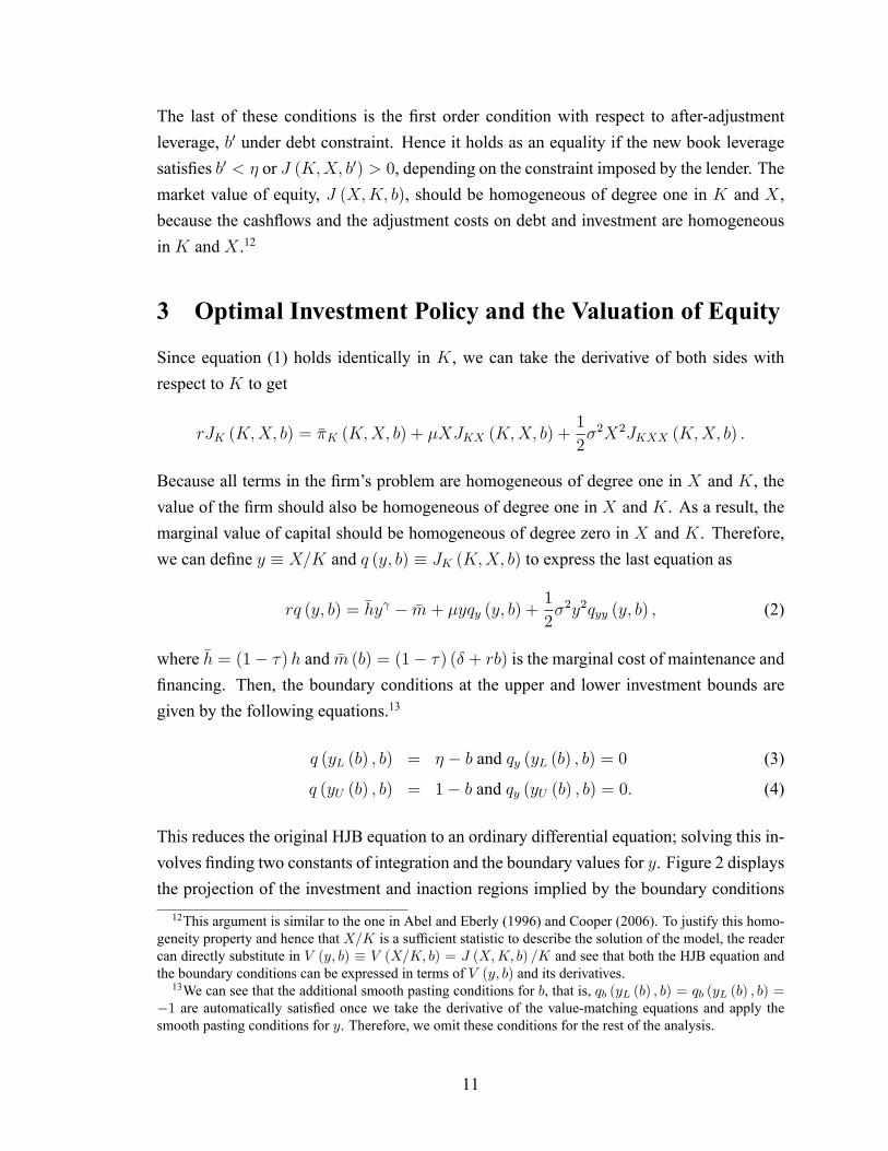
Figure 3: Expected returns vs. book-to-market ratio using the estimated parameters.Source: Author's calculations
r �S �X �A �i � � �0.02 0.38 -0.028 0.05 0.15 0.20 0.40 0.35 0.07
Table 1: Calibration of model parameters. Source: Author's calculations.
The appendix shows the derivation of the closed-form solution for the long-run station-ary distribution of book-to-market values implied by the model. For estimation purposes,I make the counterfactual assumption that book-to-market values are serially and cross-sectionally independent and identically distributed, because the complex nature of the fullinformation maximum likelihood function would require resorting to simulated maximumlikelihood, which would be computationally expensive. Hayashi (2000) shows that the re-sulting quasi-maximum likelihood estimator is indeed consistent, and it is a safe approach,given the high number of �rm-year observations in Compustat.The resulting estimation values are presented in Table 1, while Figure 3 gives the rela-
tionship between conditional expected stock returns and the book-to-market values impliedby the calibration.The standard errors are to be calculated using a bootstrap procedure andignored for now. Indeed, we see that the Modigliani and Miller channel of leverage dom-inates the investment channel, because the equity returns are increasing in book-to-marketvalues.Using this calibration we can also immediately decompose the contribution of lever-
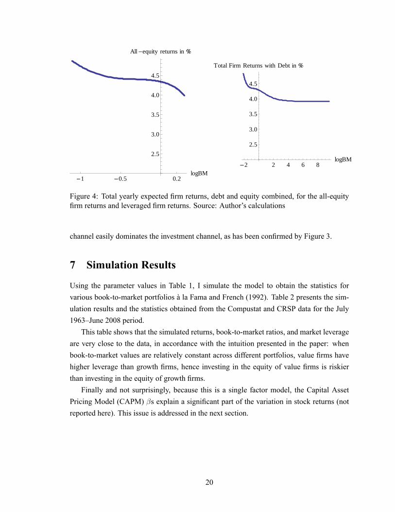
age to stock returns through investment and Modigliani-Miller channels. Figure 4 showsthat introducing debt has hardly any effect on business risk; hence the Modigliani-Miller
19
1 0.5 0.2logBM
2.5
3.0
3.5
4.0
4.5
All equity returns in
2 2 4 6 8logBM
2.5
3.0
3.5
4.0
4.5
Total Firm Returns with Debt in
Figure 4: Total yearly expected �rm returns, debt and equity combined, for the all-equity�rm returns and leveraged �rm returns. Source: Author's calculations
channel easily dominates the investment channel, as has been con�rmed by Figure 3.
7 Simulation Results
Using the parameter values in Table 1, I simulate the model to obtain the statistics forvarious book-to-market portfolios à la Fama and French (1992). Table 2 presents the sim-ulation results and the statistics obtained from the Compustat and CRSP data for the July1963�June 2008 period.This table shows that the simulated returns, book-to-market ratios, and market leverage
are very close to the data, in accordance with the intuition presented in the paper: whenbook-to-market values are relatively constant across different portfolios, value �rms havehigher leverage than growth �rms, hence investing in the equity of value �rms is riskierthan investing in the equity of growth �rms.Finally and not surprisingly, because this is a single factor model, the Capital Asset
Pricing Model (CAPM) �s explain a signi�cant part of the variation in stock returns (notreported here). This issue is addressed in the next section.
20

Portfolio Return BE/ME ML. BL. Return BE/ME ML. BL.1 8.48 0.16 0.17 0.48 9.48 0.19 0.14 0.502 10.61 0.32 0.24 0.45 11.44 0.37 0.24 0.503 12.14 0.45 0.31 0.47 12.38 0.53 0.31 0.504 12.51 0.57 0.38 0.49 12.64 0.58 0.36 0.505 14.12 0.70 0.43 0.51 14.68 0.83 0.41 0.506 15.51 0.83 0.48 0.53 15.26 0.86 0.45 0.507 17.14 0.99 0.51 0.52 17.96 1.19 0.50 0.508 17.72 1.19 0.55 0.52 18.06 1.36 0.54 0.509 19.93 1.51 0.58 0.51 20.30 1.53 0.60 0.50
10 24.27 2.85 0.66 0.51 28.56 3.29 0.74 0.50
Data Model
Table 2: Data versus simulation results with estimated parameters. The simulation resultsare the average of 25 simulations with 4000 �rms and 2500 periods each. The �rst 1500 pe-riods have been discarded to allow the system to converge to its steady state. The portfoliosare sorted according to their book-to-market values in order to form 10 portfolios everymonth, as done by Cooper (2006), instead of every year, as in Fama and French (1992).Yearly sorting does not change the results in a signi�cant way. The results are averagesacross simulations. Simulated returns are adjusted upwards for in�ation. Source: CRSPand Compustat merged database and author's calculations.
8 Time-Varying Price of Capital
One property of the model is that there is only a single systematic shock, and hence theconditional CAPM holds. Although the unconditional version of the CAPM cannot explainperfectly the differences in stock returns, it still explains a signi�cant fraction�more thanwhat is predicted by the data. This is a common property of the production-based modelsthat try to explain cross-sectional variation in stock returns with only one shock.19 However,one reason the value premium is a puzzle is that it cannot be explained by the CAPM.Many investor-based models like the inter-temporal capital asset pricing model (ICAPM),as studied by Merton (1973), Campbell and Vuolteenaho (2004), and Lettau and Wachter(2007), suggest that the CAPM fails because it does not price a risk factor correctly�inparticular the shocks to discount rate.Following their footsteps, in order to facilitate the violation of the conditional CAPM,
this section introduces an additional systematic shock. In my case, this shock affects pricesof capital goods. I show that this extended model can be reduced to a version of the originalmodel where the CAPM does not capture correctly the risk prices for capital goods price19Examples are Carlson, Fisher, and Giammarino (2004), Zhang (2005) and Berk, Green, and Naik (1999),
among others.
21

and productivity risk. As a result, the conditional CAPM betas do not line up with cross-sectional stock returns and, even more interestingly, conditional betas may be negativelyrelated to book-to-market ratios in some periods.I assume that the price of capital follows a geometric Brownian motion,20 that is,
dPtPt
= �Pdt+ �PdwP :
For this process, �P < 0 implies that increasing the capacity becomes cheaper over time,creating a vintage capital effect. We can write the problem of the �rm as
W (Kt; X̂t; Pt) = maxfdUt+s;dLt+s;dbt+sg
Et
ZSt+sSt��Kt+s; X̂t+s; Pt+s
�ds
+
ZSt+sSt
[(1� b)Pt+sdUt+s + (� � b)Pt+sdLt+s]
+1X
s2fs:dbt+s 6=0g
St+sSt
[dbt+s � c(bt+s + dbt+s)]Pt+sKt+s
subject to
dKt = dUt � dLtdStSt
= �rdt� �SAdwA;t + �SPdwP;t
dX̂t
X̂t
= �Adt+ �AdwA;t + �idwi;t
dPtPt
= �Pdt+ �PdwP ;
where
��Kt; X̂t; Pt
�� (1� �)
�h
1� X̂tK1� t � �PtKt � rbPtKt
�+ �̂P bPtKt:
The new term �̂P bPtKt appears because of the changes in the amount of debt as a result ofchanges in the price of capital, where �̂P = �P + �SP�P is the risk-adjusted drift of theprice process. Intuitively, operating capital acts as an asset that provides an instantaneousreturn of dP=P as a result of the debt agreement and price movements and �̂P is the risk-adjusted value of this return. I assume that the risk prices of X̂ and P have opposite signs,because good times are characterized by higher productivity and lower input prices.20For example, this process may come from a perfectly competitive industry that produces capital goods,
with a linear production function subject to technology shocks that follow a geometric Brownian motion.
22
Note that this problem is linearly homogeneous in X̂t and Pt, since both variablesfollow a geometric Brownian motion and enter linearly into the problem. Therefore, Ican divide everything by Pt and de�ne X
t � X̂=Pt, � (K;X) � �(K; X̂; P )=P andJ (K;X) � W (K; X̂; P )=P . This will give us the following Hamilton-Jacobi-Bellmanequation in the inaction region
(r � �̂P ) J = � (K;X) + �XJX +1
2�2X2JXX ;
where
� =1
(�̂A � �̂P ) +
1
2
�1
� 1�1
��2P + �
2A + �
2i
��2 =
1
2��2P + �
2A + �
2i
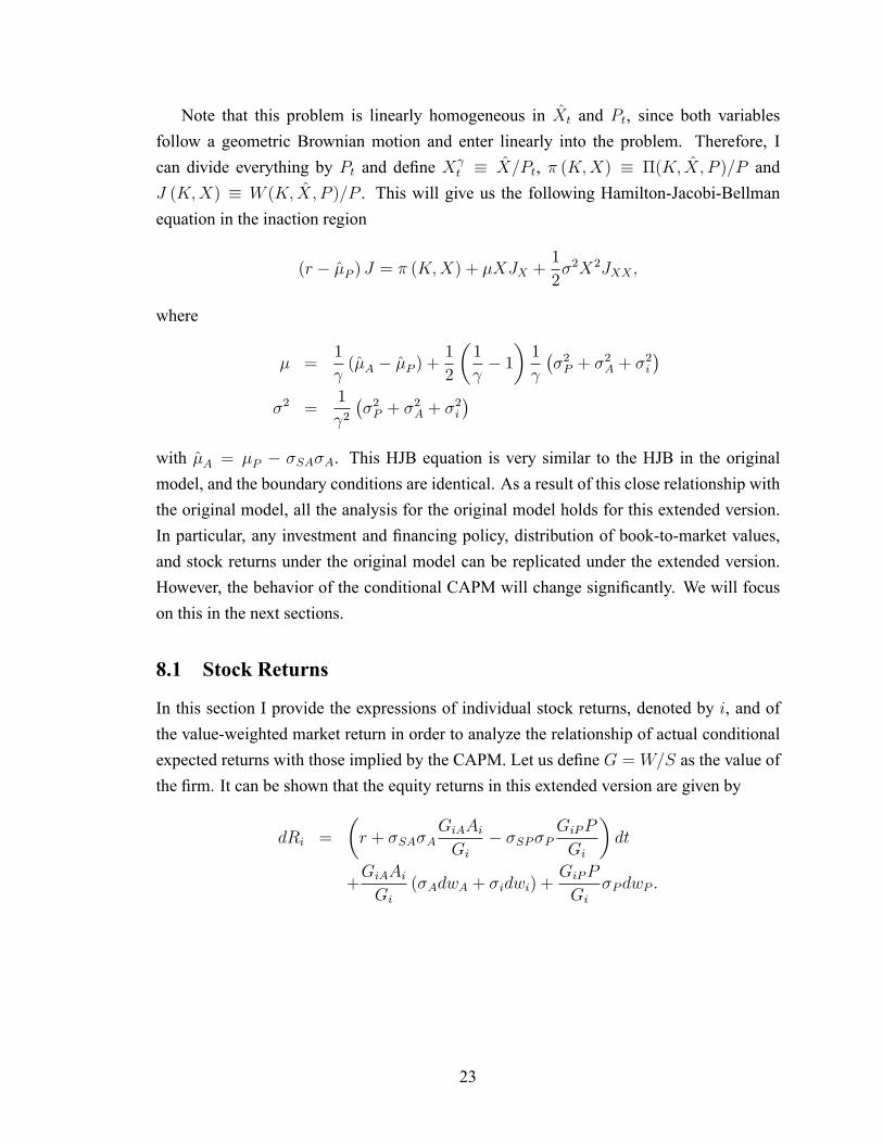
�with �̂A = �P � �SA�A. This HJB equation is very similar to the HJB in the originalmodel, and the boundary conditions are identical. As a result of this close relationship withthe original model, all the analysis for the original model holds for this extended version.In particular, any investment and �nancing policy, distribution of book-to-market values,and stock returns under the original model can be replicated under the extended version.However, the behavior of the conditional CAPM will change signi�cantly. We will focuson this in the next sections.
8.1 Stock Returns
In this section I provide the expressions of individual stock returns, denoted by i, and ofthe value-weighted market return in order to analyze the relationship of actual conditionalexpected returns with those implied by the CAPM. Let us de�ne G = W=S as the value ofthe �rm. It can be shown that the equity returns in this extended version are given by
dRi =
�r + �SA�A
GiAAiGi
� �SP�PGiPP
Gi
�dt
+GiAAiGi
(�AdwA + �idwi) +GiPP
Gi�PdwP :
23

Due the homogeneity of G (K;A; P ) in A and P , we have GiPPGi
=�1� GiAAi
Gi
�. Using
this and the de�nition of J , we can write the last equation as
dRi =
�r + �SA�A
JiXXi
Ji� �SP�P
�1� JiXXi
Ji
��dt
+JiXXi
Ji(�AdwA + �idwi) +
�1� JiXXi
Ji
��PdwP :
Note that, similar to the original model, the effect of book-to-market value is captured bythe elasticity of the market value of equity with respect to productivity shocks JiXXi=Ji.Using individual stock returns, we can derive the market return as
dRm =
�r + �SA�A
RiXiJiX (Ki; Xi) di
RiJi (Ki; Xi) di
� �SP�P�1�
RiXiJiX (Ki; Xi) di
RiJi (Ki; Xi) di
��dt
+
RiXiJiX (Ki; Xi) di
RiJi (Ki; Xi) di
�AdwA +
�1�
RiXiJiX (Ki; Xi) di
RiJi (Ki; Xi) di
��PdwP :
8.2 Market Beta and Failure of the Conditional CAPM
Using the individual �rm and value-weighted market returns presented above, I will showthe failure of the conditional CAPM. For the sake of simplifying the notation, de�ne
�m =
RiXiJiX (Ki; Xi) di
RiJi (Ki; Xi) di
�i =JiXXi
Ji:
Using the formulas above, we can calculate the conditional market beta as
�i =cov (dRm; dRi)
var (dRm)
=�i�m�
2A + (1��i) (1��m)�
2P
�2m�
2A + (1��m)
2 �2P:
Then, the expected instantaneous return implied by the conditional CAPM is not equal toconditional expected returns, that is,
�iE [dRm � rdt] =�i�m�
2A + (1��i) (1��m)�
2P
�2m�
2A + (1��m)
2 �2P[�m (�SA�A + �SP�P )� �SP�P ] dt
6= [�i (�SA�A + �SP�P )� �SP�P ] dt = E [dRi � rdt] ;
24

which implies the failure of the conditional CAPM.More interestingly, it is possible that a �rm with higher returns has a lower beta. To see
this, rewrite beta as
�i =�i [�m (�
2A + �
2P )� �2P ] + (1��m)�
2P
�2m�
2A + (1��m)
2 �2P:
While the expected return is increasing in �i (which leads to a value premium) we have@�i=@�i < 0 if �2A=�2P < (1��m) =�m, which holds when �m is suf�ciently small.Note that
RiXiJiX(Ki;Xi)diRi Ji(Ki;Xi)di
= 1 �RiKiJiK(Ki;Xi)diRi Ji(Ki;Xi)di
, due to homogeneity, and hence �m issmall when JK is particularly high, that is, during good times. This implies that the excessmarket return and the conditional market betas are countercyclical.In this model, the CAPM fails because there is a systematic factor that the CAPM does
not price correctly; that is, the shocks to the price of capital goods. The bottom line isthat we can generate the failure of the CAPM with relative ease compared with the effortinvolved in generating the correct cross-sectional distribution of stock returns and book-to-market values simultaneously.
9 Conclusion
This paper presents a dynamic model of the �rm with limited capital irreversibility and in-complete debt contracts in order to analyze the effects of �nancial leverage on investmentand explain the cross-sectional differences in equity returns. This model can capture sev-eral regularities in the corporate �nance and asset pricing literature in a parsimonious andtractable way.Introducing debt into production-based asset pricing models opens several possibilities.
For example, the model presented here could be extended with time-varying interest rates ina similar framework toMerton's (1973) intertemporal capital asset pricing model (ICAPM).This would serve two purposes. First, it would decrease the explanatory power of theconditional market beta for stock returns and get us one step closer to solving the valuepremium puzzle. Second, because �rms with a high book-to-market ratio also have higherleverage, they will have greater exposure to interest rate shocks, further reinforcing thevalue premium. I hope that this paper will stimulate future research in this direction.
25

10 References
Abel, Andrew B. and Janice C. Eberly. 1995. �Optimal Investment with Costly Reversibil-ity.� Working Paper 5091. Cambridge, MA: National Bureau of Economic Research.Abel, Andrew B. and Janice C. Eberly. 1996. �Optimal Investment with Costly Reversibil-ity.� Review of Economic Studies 63(4): 581�593.Berk, Jonathan B., Richard C. Green, and Vasant Naik. 1999. �Optimal investment, growthoptions and security returns.� Journal of Finance (54):1153�1607.Bertola, Giuseppe and Ricardo J. Caballero. 1990. �Kinked Adjustment Costs and Aggre-gate Dynamics.� NBER Macroeconomics Annual 1990 5: 237�288.Black, Fischer. 1972. �Capital Market Equilibrium with Restricted Borrowing.� Journal ofBusiness 45(3): 444�455.Campbell, John Y. and Tuomo Vuolteenaho. 2004. �Bad Beta, Good Beta.� AmericanEconomic Review 94(5): 1249�1275.Carlson, Murray D., Adlai J. Fisher, and Ron Giammarino. 2004. �Corporate Investmentand Asset Price Dynamics: Implications for the Cross Section of Returns.� Journal ofFinance 59(6): 2577�2603.Cooper, Ilan. 2006. �Asset Pricing Implications of Nonconvex Adjustment Costs andIrreversibility of Investment.� Journal of Finance 61(1): 139�170.Dixit, Avinash K. 1993. The Art of Smooth Pasting. Chur, Switzerland: Harwood Acad-emic Publishers.Fischer, Edwin O., Robert Heinkel, and Josef Zechner. 1989. �Dynamic Capital StructureChoice: Theory and Tests.� The Journal of Finance 44(1): 19�40.Fama, Eugene F. and Kenneth R. French. 1992. �The Cross-Section of Expected StockReturns.� Journal of Finance 47: 427�465.Fama, Eugene F. and Kenneth R. French. 1993. �Common Risk Factors in the Returns onStocks and Bonds.� Journal of Financial Economics 33: 3�56.Gomes, Joao F. and Lukas Schmid. 2009. �Levered Returns.� Working Paper, Universityof Pennsylvania.Grinblatt, Mark and Sheridan Titman. 2001. Financial Markets and Corporate Strategy,2nd Edition. McGraw-Hill.Hall, Robert E. 2004. �Measuring Factor Adjustment Costs.� Quarterly Journal of Eco-nomics 119(3): 899�927.Hayashi, Fumio. 2000. Econometrics. Princeton, NJ: Princeton University Press.Lintner, John. 1965. �The Valuation of Risk Assets and the Selection of Risky Investmentsin Stock Portfolios and Capital Budgets.� Review of Economics and Statistics 47(1): 221�245.
26

Livdan, Dmitry, Horacio Sapriza, and Lu Zhang. 2009. �Financially Constrained StockReturns.� Journal of Finance, forthcoming.Lettau, Martin, and Jessica A. Wachter. 2007. �Why is Long-Horizon Equity Less Risky?A Duration-Based Explanation of the Value Premium.� Journal of Finance 62: 55�92.Merton, Robert C. 1973. �An Intertemporal Capital Asset Pricing Model.� Econometrica41(5): 867�887.Modigliani, Franco andMerton H.Miller. 1958. �The Cost of Capital, Corporation Financeand the Theory of Investment.� The American Economic Review 48(3): 261�297.Sharpe, William F. 1964. �Capital Asset Prices: A Theory of Market Equilibrium underConditions of Risk.� Journal of Finance 19(3): 425�442.Taylor, Jack. 2003. �Corporation Income Tax Brackets and Rates,1909�2002.� StatisticsIncome Bulletin, Fall.(http://www.irs.gov/pub/irs-soi//99corate.pdf).Welch, Ivo. 2004. �Capital Structure and Stock Returns.� Journal of Political Economy112(1): 106�131.Zhang, Lu. 2005. �The Value Premium.� Journal of Finance 60(1): 67�103.
11 Appendix
11.1 Market Value and Stock Returns with Irreversibility and Finan-cial Leverage
We can simplify our problem by de�ning ~q (y; b) � q (y; b) + �m=r. Therefore, equations(2), (3), and (4) can be rewritten as
r~q (y; b) = �hy + �y~qy (y; b) +1
2�2y2~qyy (y; b)
~q (yL (b) ; b) = � � b+ �m (b) =r � l (b) and ~qy (yL (b) ; b) = 0~q (yU (b) ; b) = 1� b+ �m (b) =r � u (b) and ~qy (yU (b) ; b) = 0:
This makes the solution of the differential equation similar to the one in Abel and Eberly(1996), which is a special case of my model that excludes leverage and the risk preferencesof investors. Following their analysis, I de�ne the following functions
� (x) = �12�2x2 �
��� 1
2�2�x+ r
� (x) =x�P � x x�P � x�N
� (x) =1
� ( )
�1�
�N� (x)�
�P[1� � (x)]
�;
27

where �P and �N are the roots of the quadratic equation � (x) = 0 and satisfy �P > 1 > > 0 > �N . Then, the solution of this differential equation should be of the form
~q (y; b) = Hy + CP (b) y�P + CN (b) y
�N :
The reason is that b appears only in the boundary conditions for ~q but not in the differentialequation.De�ne H ( ) � �h=� ( ) and G (b) � yU (b) =yL (b). Then, the solution of the differen-
tial equation for ~q (y; b) is given by21
~q (y; b) = H ( ) yL (b)
���
y
yL (b)
� �
�P[1� � (G (b))]
�y
yL (b)
��P�
�N� (G (b))
�y
yL (b)
��N�;
where G (b) is implicitly de�ned by
u (b)
l (b)� (G (b))�G (b) � (1=G (b)) = 0 (8)
and the values of boundaries are given by
�hyU (b) =
u (b)
� (1=G (b))and �hyL (b) =
l (b)
� (1=G (b)):
Using this solution, the value function can be found by simply integrating q (X=K)over K to get22
J (K;X; b)
= H ( ) y L
�1
1� X K1�
yL (b) �
�P
1� � (G)1� �P
X�PK1��P
yL (b)�P �
�N
� (G)
1� �NX�NK1��N
yL (b)�N
�� �m (b)
rK
= JAP + JG + JD � �m (b)
rK:
Now we focus on stock returns. Apply Ito's Lemma to equity value in the inaction21The solution is identical to that of Abel and Eberly (1996) once the purchase and resale prices of capital
in their model are substituted with u (b) and l (b), respectively. Therefore, I omit the lengthy details of thecalculus that leads to the solution, but they are available upon request.22Direct integration of q (y) would yield a constant of integration that should have the formDX (b)X , due
to the homogeneity property of the value function. However, direct substitution of J (X;K) into the HJBequation shows immediately that DX (b) should be zero.
28

region, J (K;X)
dJ =
��XXJX +
1
2�2X2JXX
�dt+ �XJXdw:
Use the relationship � = �X��S�A and the HJB equation rJ = �+�XJX+ 12�2X2JXX
to get1
dtE
�dJ
J
�= ��
J+ r + �S
JXX
J:
Plugging this expression into the return formula gives the excess returns
1
dtE (dR)� r = 1
dtE
��dt+ dJ
J
�� r = �S�A
JXX
J:
To show that the returns are increasing in y, �rst note that we can write the excessreturns as
1
dtE (dR)� r =
�
JAP
J + �m=rK+ �P
JG (K;X)
J + �m=rK+ �N
JD (K;X)
J + �m=rK
��1 +
�m=rK
J
��S�A
= ( sAP + �P sG + �NsD)
�1 +
�m=rK
J
��S�A;
where the �rst term decomposes the total business risk into assets-in-place, the growthoption and the disinvestment option, while the second term captures the Modigliani-Millereffect.
11.2 Proof of Proposition 2
From the previous section, we know that the following equation builds the connectionbetween the investment and disinvestment boundary and �nancial leverage
u (b)
l (b)� (G (b))�G (b) � (1=G (b)) = 0; (9)
which we can rewrite asu (b)
l (b)=G (b) � (1=G (b))
� (G (b)):
It is easy to show that the left side of this equation is increasing in b, and hence the rightside of the equation should be increasing in b. Abel and Eberly (1995) show in a lengthyand tedious proof that G
�(1=G)�(G)
is increasing in G. Suppose G0 (b) � 0. Then, the left sidewould be weakly decreasing in b, causing a contradiction.
29
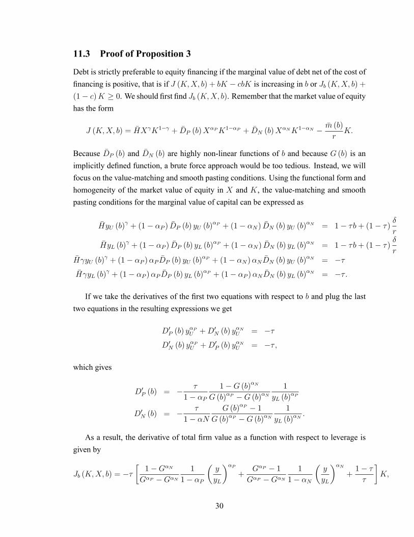
11.3 Proof of Proposition 3
Debt is strictly preferable to equity �nancing if the marginal value of debt net of the cost of�nancing is positive, that is if J (K;X; b) + bK � cbK is increasing in b or Jb (K;X; b) +(1� c)K � 0. We should �rst �nd Jb (K;X; b). Remember that the market value of equityhas the form
J (K;X; b) = �HX K1� + �DP (b)X�PK1��P + �DN (b)X
�NK1��N � �m (b)
rK:
Because �DP (b) and �DN (b) are highly non-linear functions of b and because G (b) is animplicitly de�ned function, a brute force approach would be too tedious. Instead, we willfocus on the value-matching and smooth pasting conditions. Using the functional form andhomogeneity of the market value of equity in X and K, the value-matching and smoothpasting conditions for the marginal value of capital can be expressed as
�HyU (b) + (1� �P ) �DP (b) yU (b)
�P + (1� �N) �DN (b) yU (b)�N = 1� �b+ (1� �) �
r
�HyL (b) + (1� �P ) �DP (b) yL (b)
�P + (1� �N) �DN (b) yL (b)�N = 1� �b+ (1� �) �
r�H yU (b)
+ (1� �P )�P �DP (b) yU (b)�P + (1� �N)�N �DN (b) yU (b)
�N = ���H yL (b)
+ (1� �P )�P �DP (b) yL (b)�P + (1� �P )�N �DN (b) yL (b)
�N = �� :
If we take the derivatives of the �rst two equations with respect to b and plug the lasttwo equations in the resulting expressions we get
D0P (b) y
�PU +D0
N (b) y�NU = ��
D0N (b) y
�PU +D0
P (b) y�NU = �� ;
which gives
D0P (b) = � �
1� �P1�G (b)�N
G (b)�P �G (b)�N1
yL (b)�P
D0N (b) = � �
1� �NG (b)�P � 1
G (b)�P �G (b)�N1
yL (b)�N :
As a result, the derivative of total �rm value as a function with respect to leverage isgiven by
Jb (K;X; b) = ���1�G�NG�P �G�N
1
1� �P
�y
yL
��P+
G�P � 1G�P �G�N
1
1� �N
�y
yL
��N+1� ��
�K;
30

where b has been dropped in G (b) for the sake of brevity. Therefore the marginal value ofdebt is given by
Jb + (1� c)K = �
�1� 1�G�N
G�P �G�N1
1� �P
�y
yL
��P� G�P � 1G�P �G�N
1
1� �N
�y
yL
��N�K
�cK:
Since G > 1 and �P > 1 > 0 > �N , the term in square brackets is decreasing in y.Therefore, debt is the preferred for of �nancing at every state if Jb + (1� c)K > 0 aty = yL. Substituting y = yL above reduces our condition to
c < c� (b) = �
�1� 1�G�N
G�P �G�N1
1� �P� G�P � 1G�P �G�N
1
1� �N
�:
Since G > 1 and �P > 1 > 0 > �N , the second term is on the right side is negative andthe third term is less than 1. Moreover, the right side of this equation is decreasing in G,and we already know from the proof of the previous proposition thatG0 (b) > 0. Therefore,c� (b) > 0 and c�0 (b) < 0. The minimum for c� (b) is then attained when G ! 1, that is,c� = 1�1= (1� �N). So, if c < 1�1= (1� �N), then debt is always preferable regardlessof state and degree of irreversibility.
11.4 Proof of Proposition 4
Using the results from the last section we have
Jb +K = �
�1� 1�G�N
G�P �G�N1
1� �P
�y
yL
��P� G�P � 1G�P �G�N
1
1� �N
�y
yL
��N�K;
which attains its minimum value for y = yL. So, it is enough to show that this value ispositive once we substitute y = yL, i.e. that
�
�1� 1�G�N
G�P �G�N1
1� �P� G�P � 1G�P �G�N
1
1� �N
�> 0:
Again, since G > 1 and �P > 1 > 0 > �N , the second term is on the right side is negativeand the third term is less than 1. Therefore, the term in square brackets should be positive.Since Jb+K > 0, one of the smooth pasting conditions at debt adjustment is not satis�ed,and hence it is not optimal to readjust debt.
31

11.5 Market Value and Stock Returns with Investment IrreversibilityOnly
The market value of equity under this setting is the same, except that we should set b = � =0. Let H ( ) � h=� ( ) and G � yU=yL. Then, the solution of the differential equation forq (y) where y � X=K is given by
q (y) = H ( ) y L
��y
yL
� �
�P[1� � (G)]
�y
yL
��P�
�N� (G)
�y
yL
��N�;
where G is the solution of1
�� (G)�G �
�G�1
�= 0:
Using this solution, the value function can be found by simply integrating q (X=K) overKto get23
J (K;X)
= H ( ) y L
�1
1� X K1�
y L�
�P
1� � (G)1� �P
X�PK1��P
y�PL�
�N
� (G)
1� �NX�NK1��N
y�NL
�= JAP + JG + JD:
To show that the returns are increasing in y, �rst note that we can write the excessreturns as
1
dtE (dR)� r =
� JAP (K;X)
J (K;X)+ �P
JG (K;X)
J (K;X)+ �N
JD (K;X)
J (K;X)
��S�A
=
� JAP (1; y)
J (1; y)+ �P
JG (1; y)
J (1; y)+ �N
JD (1; y)
J (1; y)
��S�A
=
� + (�P � )
JG (1; y)
J (1; y)+ (�N � )
JD (1; y)
J (1; y)
��S�A:
Now, it is easy to show that JG (1; y) =J (1; y) is increasing in y and JD (1; y) =J (1; y) isdecreasing in y by taking the derivatives. Since �P � > 0 and �N � < 0, this lastexpression should be increasing in y.23Direct integration of q (y) would yield a constant of integration that should depend linearly on X due
to the homogeneity property of the value function. However, direct substitution of J (X;K) in to the HJBequation shows immediately that this term should be zero.
32
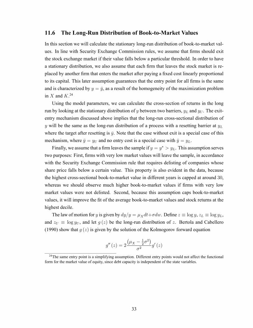
11.6 The Long-Run Distribution of Book-to-Market Values
In this section we will calculate the stationary long-run distribution of book-to-market val-ues. In line with Security Exchange Commission rules, we assume that �rms should exitthe stock exchange market if their value falls below a particular threshold. In order to havea stationary distribution, we also assume that each �rm that leaves the stock market is re-placed by another �rm that enters the market after paying a �xed cost linearly proportionalto its capital. This later assumption guarantees that the entry point for all �rms is the sameand is characterized by y = �y, as a result of the homogeneity of the maximization problemin X and K.24
Using the model parameters, we can calculate the cross-section of returns in the longrun by looking at the stationary distribution of y between two barriers, yL and yU . The exit-entry mechanism discussed above implies that the long-run cross-sectional distribution ofy will be the same as the long-run distribution of a process with a resetting barrier at yLwhere the target after resetting is �y. Note that the case without exit is a special case of thismechanism, where �y = yU and no entry cost is a special case with �y = yL.Finally, we assume that a �rm leaves the sample if y = y� > yL. This assumption serves
two purposes: First, �rms with very low market values will leave the sample, in accordancewith the Security Exchange Commission rule that requires delisting of companies whoseshare price falls below a certain value. This property is also evident in the data, becausethe highest cross-sectional book-to-market value in different years is capped at around 30,whereas we should observe much higher book-to-market values if �rms with very lowmarket values were not delisted. Second, because this assumption caps book-to-marketvalues, it will improve the �t of the average book-to-market values and stock returns at thehighest decile.The law of motion for y is given by dy=y = �Xdt+�dw. De�ne z � log y, zL � log yL,
and zU � log yU , and let g (z) be the long-run distribution of z. Bertola and Cabellero(1990) show that g (z) is given by the solution of the Kolmogorov forward equation
g00 (z) = 2
��X � 1
2�2�
�2g0 (z)
24The same entry point is a simplifying assumption. Different entry points would not affect the functionalform for the market value of equity, since debt capacity is independent of the state variables.
33

separately for the regions [zL; �z) and (�z; zU ] with the following boundary conditions
g0��z��= g
��z+�+ g0
�z+L�
g0 (zU) = 2
��X � 1
2�2�
�2g (zU)
g (z�) = 0;
where g (z+) is the right limit and g (z�) is the left limit of the distribution function. Wealso have the integral condition Z zU
zL
g (z) dz = 1:
Once we �nd g (z), we can �nd the distribution of y using the transformation ' (y) =g (ln y). A little algebra shows that the long-run distribution of y is given by
' (y) =
8>><>>:�A1y
(2�X��2)=�2 +B1
�=y if y� < y < �y
A2y(2�X��2)=�2�1 if �y � y < yU
0 otherwise;
where A1; A2 and B1 satisfy
(y�)(2�X��2)=�2 A1 +B1 = 0�
�y(2�X��2)=�2 � (y�)(2�X��
2)=�2�A1 � �y(2�X��
2)=�2A2 = 0
�y(2�X��2)=�2 � (y�)(2�X��
2)=�2
(2�X � �2) =�2A1 +
y(2�X��2)=�2U � �y(2�X��2)=�2
(2�X � �2) =�2A2 + ln
��y
y�
�B1 = 1:
Then, we can write market-to-book values as J= (1� b)K = V (y) = (1� b). Oncewe de�ne the function ! (y) = V (y) = (1� b), the long-run distribution of market-to-bookvalues,mb, is given by
f (mb) = '�!�1 (mb)
� ����d!�1 (mb)d (mb)
����for V (yU) = (1� b) � mb � V (yL) = (1� b), and zero otherwise.Once we have the long-run distribution of book-to-market values, I use the long-run dis-
tribution derived from the data in order to estimate the model parameters using maximumlikelihood.
34