Embed Size (px)
Citation preview
Contents
Overview 1
1. The Global Financial Environment 5 Box A: Ongoing Financial Regulatory Reform in China 19
2. Household and Business Finances 23 Box B: The Impact of Lending Standards on Loan Sizes 32
Box C: Vulnerable Households and Financial Stress 37
3. The Australian Financial System 41 Box D: Cyber Risk 55
4. Regulatory Developments 59 Box E: The Council of Financial Regulators 69
5. Assessing the Effects of Housing Lending Policy Measures 75
Copyright and Disclaimer Notices 89
O C TO BER 2018
Financial Stability Review

The material in this Financial Stability Review was finalised on 11 October 2018 and uses data through to 10 October.
The Review is published semiannually and is available on the Reserve Bank’s website (www.rba.gov.au). The next Review is due for release in April 2019. For copyright and disclaimer notices relating to data in the Review, see page 89 and the Bank’s website.
The graphs in this publication were generated using Mathematica.
Financial Stability Review enquiries:
Secretary’s DepartmentTel: +61 29551 8111Fax: +61 2 9551 8033Email: [email protected]
ISSN 1449-3896 (Print)ISSN 1449-5260 (Online)
F I N A N C I A L S TA B I L I T Y R E V I E W | O C TO B E R 2018 1
Overview
Global economic and financial conditions are generally positiveGrowth has been above trend rates in the major advanced economies and in most of Australia’s major trading partners. Central banks in the United States and some other advanced economies have begun to remove the exceptional monetary policy stimulus. But monetary policy has remained very expansionary in the euro area and Japan. Overall, global financial conditions remain highly accommodative. The tightening in the United States and divergent monetary policies have not disrupted financial markets as central banks have been careful to clearly communicate their expected paths for policy. Overall, positive economic and stable financial market conditions have supported financial stability. However, the extended period of low interest rates has seen some financial stability risks emerge. Notably compensation for risk is very low with asset prices in a range of markets at high levels, underpinned by low long-term interest rates. Household, corporate and sovereign debt has also risen to high levels in some jurisdictions. For emerging market economies – especially those with structural or cyclical vulnerabilities – there are concerns about the implications of a tightening in financial conditions in the advanced economies.
The Australian economy is improving while the housing market has slowedIn Australia, economic growth has been strong, with unemployment falling. Wages growth has been low, but strong employment growth has helped to support household incomes. Similarly, businesses are earning solid profits. Given most businesses have low gearing, few have difficulty in servicing their debt.
Conditions in the housing market have eased, reflecting shifts in both supply and demand. Sentiment towards the housing market has become more cautious and this has been reflected in a slowing in demand for housing finance, particularly from investors. This has been reinforced by stricter lending conditions as a result of actions by regulators over the past few years, notably on investor, interest-only and high loan-to-valuation loans. The prudential measures were introduced because of concerns about the growth of riskier types of housing lending, particularly given that the level of household debt was already high. The banks have also applied their own lending standards more diligently. Most borrowers do not take out the maximum loan possible and so the vast majority of prospective borrowers have not been affected by these changes. However, some existing borrowers may find they do not meet new lending standards and so have difficulty refinancing. Similarly, while most borrowers with loans transitioning from interest-only to principal and interest payments are well placed
R E S E R V E B A N K O F AU S T R A L I A2
to meet the higher payments, a small share could struggle. There has been only a small uptick in non-performing housing loans, primarily in Western Australia; overall, rates of non-performing loans remain very low. For non-residential commercial property, valuations continue to rise in the eastern states and yields have fallen further, in line with high global asset prices underpinned by low long-term interest rates.
There are some vulnerabilities for Australian financial stability
External exposure
Australia would be sensitive to a sharp contraction in global growth or dislocation in global financial markets because of the importance of trade and capital inflows. A worsening in external conditions could see a downturn in the domestic economy, reduced availability and higher cost of offshore funding and falls in asset prices, with a resulting deterioration in the performance of borrowers and lenders. In the current environment, a range of possible triggers could precipitate a global economic downturn. An escalation of trade protection could see a sharp fall in trade, business confidence and investment. A fall in economic growth in China, possibly stemming from the high level of debt and the complex and obscure linkages in the financial system, would spread to many economies, including those in Asia with strong economic links to Australia. Global financial market volatility and risk premia could rise for a range of reasons. Contagion among emerging market economies could spread from Argentina and Turkey, or banking and sovereign debt problems in Europe could escalate from Italy. And an increase in risk aversion could see a jump in premia in long-term interest rates undermining high asset valuations.
Household debt
The level of household debt in Australia is high relative to its history and to other countries. Directly, this does not appear to be a large risk to the financial system. The majority of this debt is well secured, with only a small portion having a high loan-to-valuation ratio. Further, most of the debt is owed by households that appear well placed to repay the debt. Rather, the risks of high household debt appear to be to the economy. Highly indebted households could cut back their consumption if their financial position were to be less secure. Given high household debt, these effects could potentially be substantial for the aggregate economy, indirectly affecting the financial system.
The housing slowdown and credit supply
The housing market has slowed in part reflecting policy measures over the past few years. After the substantial rise in housing debt and prices over the past decade, this is a positive development for financial stability. But if the housing market were to contract sharply, this would result in some borrowers having negative equity. It is possible, although not likely, that an excessive tightening in lending standards could exacerbate the current housing slowdown. Most of the tightening in lending standards prompted by regulators is already in place, however, banks are further adjusting their own lending standards. A tightening in banks’ risk appetite could particularly affect housing developers and so construction.
Bank culture and operational risk
In the past year inquiries into the Australian banks have exposed deficiencies in operational risk management stemming from poor culture. The response of financial institutions will, over time, contribute to a more resilient financial
F I N A N C I A L S TA B I L I T Y R E V I E W | O C TO B E R 2018 3
system. But the evidence presented highlights the deficiencies that can arise with insufficient control of operational risk. To date, the financial implications for banks have been small, but the consequences of reputational damage could impair banks’ profitability and resilience. Cyber risk is an operational risk that warrants particular attention. Australian financial entities have not experienced significant losses or disruption from cyber attacks, but they are targets. The likelihood of a cyber attack having systemic consequences seems small, but the implications could be severe.
Financial system resilience has improvedThe resilience of Australian banks has increased over the past decade. Banks’ capital ratios are now around their ‘unquestionably strong’ prudential benchmarks. They are also around 50 per cent higher than they were a decade earlier and well within the range that has historically helped to withstand financial crises. Banks have also substantially strengthened their liquidity management in recent years, switching to more stable funding and increasing holdings of liquid assets. The strengthening of capital positions and liquidity management has reduced banks’ return on equity (ROE) relative to its historical average. However, their ROE appears to have stabilised at a level that is still high by international standards (around 12 per cent, compared with 8 per cent for large US banks).
The tightening in housing lending standards in recent years has improved the quality of the household sector’s balance sheet (see the special chapter, ‘Assessing the Effects of Housing Lending Policy Measures’). Some borrowers who would have been more likely to experience difficulty repaying their debt are now constrained
to borrow more manageable amounts. In response, lending by non-prudentially regulated lenders has picked up, but they must still comply with responsible lending laws and are too small to fully offset the tightening from other lenders. Tighter lending standards mean there should be fewer households that will struggle to service their debt if they experience falls in income or other adverse conditions. This has alleviated some of the risks from the continued rise in household indebtedness. R

R E S E R V E B A N K O F AU S T R A L I A4
F I N A N C I A L S TA B I L I T Y R E V I E W | O C TO B E R 2018 5
Australia has long been sensitive to global economic and financial trends. This sensitivity arises from trade, investment and capital flows, as well as the broader integration of the Australian financial system with global markets. Consequently, the Review pays particular attention to risks emanating from the largest economies and regions, which also dominate global financial markets, as well as those that have significant trade or financial links with Australia. These include the United States, Europe, China, Japan and New Zealand.
Recent growth in the global economy has been both solid and widespread, which is supporting global financial stability. But increasing trade protectionism poses a threat to the outlook. Asset prices in a range of markets are high and compensation for risk is low. An adverse shock could result in a broad fall in asset prices, exposing vulnerabilities that have built up in the low interest rate, low volatility environment.
High global debt levels leave households, corporates and sovereigns in a range of countries vulnerable to adverse shocks. In a number of countries, household debt levels are at historical highs relative to income, although an orderly slowdown in housing markets is underway in some cases. Debt in China is particularly high, with a large share financed through opaque non-bank lending channels. Chinese authorities’ efforts to address the associated financial stability risks are showing noticeable results, but risks remain elevated. Sovereign debt levels remain especially high in Europe, and debt sustainability concerns could quickly re-escalate. This could
1. The Global Financial Environment
undermine financial and economic stability, including by exacerbating banking sector vulnerabilities.
Ongoing external borrowing, macroeconomic imbalances and policy uncertainty have raised concerns about sovereign and corporate credit risks in some emerging market economies (EMEs). However, contagion has been limited so far, with the shift in market sentiment mostly affecting those countries with the greatest vulnerabilities.
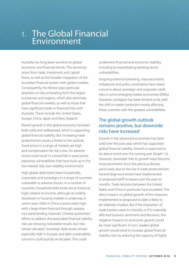
The global growth outlook remains positive, but downside risks have increasedGrowth in the advanced economies has been solid over the past year, which has supported global financial stability. Growth is expected to be above trend over the coming year (Graph 1.1). However, downside risks to growth have become more prominent since the previous Review, particularly due to the rise in trade protectionism. Several large economies have implemented or proposed tariff increases over the past six months. Trade tensions between the United States and China in particular have escalated. The direct impact on global growth of the measures implemented or proposed to date is likely to be relatively modest. But if the imposition of trade barriers were to intensify, or if it materially affected business sentiment and decisions, the negative impacts on economic growth could be more significant. In turn, weaker global growth would tend to increase global financial stability risks by reducing the capacity of highly
R E S E R V E B A N K O F AU S T R A L I A6
Evolution of GDP Forecasts*Year-average
2018
2017 20180.5
1.5
2.5
%
US
Euro area
2019
2017 20180.5
1.5
2.5
%
Japan
* Dashed lines represent the average estimates of potential growthfor 2018-19
Sources: Consensus Economics; national sources
10-year Government Bond YieldsMonthly averages
20112004 2018-150
0
150
300
450
600
bps
US
US term premium
20112004 2018-150
0
150
300
450
600
bps
UK
Germany
Japan
Sources: Bloomberg; RBA
Graph 1.1 Graph 1.2
Corporate Bond SpreadsTo government bonds with equivalent maturity
Investment grade
20112004 20180
200
400
600
bps
US dollar
Non-investment grade
20112004 20180
750
1 500
2 250
bps
Euro
Sources: ICE Data is used with permission; RBA
Graph 1.3
leveraged borrowers to service their debt. A reassessment of the global growth outlook and risk more generally could also trigger a broad fall in asset prices.
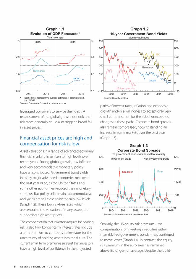
Financial asset prices are high and compensation for risk is lowAsset valuations in a range of advanced economy financial markets have risen to high levels over recent years. Strong global growth, low inflation and very accommodative monetary policy have all contributed. Government bond yields in many major advanced economies rose over the past year or so, as the United States and some other economies reduced their monetary stimulus. But policy still remains accommodative and yields are still close to historically low levels (Graph 1.2). These low risk-free rates, which are central to the valuation of many assets, are supporting high asset prices.
The compensation that investors require for bearing risk is also low. Longer-term interest rates include a term premium to compensate investors for the uncertainty of holding assets into the future. The current small term premiums suggest that investors have a high level of confidence in the projected
paths of interest rates, inflation and economic growth and/or a willingness to accept only very small compensation for the risk of unexpected changes to those paths. Corporate bond spreads also remain compressed, notwithstanding an increase in some markets over the past year (Graph 1.3).
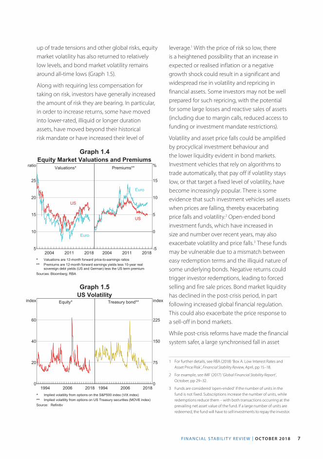
Similarly, the US equity risk premium – the compensation for investing in equities rather than risk-free government bonds – has continued to move lower (Graph 1.4). In contrast, the equity risk premium in the euro area has remained above its longer-run average. Despite the build-
F I N A N C I A L S TA B I L I T Y R E V I E W | O C TO B E R 2018 7
leverage.1 With the price of risk so low, there is a heightened possibility that an increase in expected or realised inflation or a negative growth shock could result in a significant and widespread rise in volatility and repricing in financial assets. Some investors may not be well prepared for such repricing, with the potential for some large losses and reactive sales of assets (including due to margin calls, reduced access to funding or investment mandate restrictions).
Volatility and asset price falls could be amplified by procyclical investment behaviour and the lower liquidity evident in bond markets. Investment vehicles that rely on algorithms to trade automatically, that pay off if volatility stays low, or that target a fixed level of volatility, have become increasingly popular. There is some evidence that such investment vehicles sell assets when prices are falling, thereby exacerbating price falls and volatility.2 Open-ended bond investment funds, which have increased in size and number over recent years, may also exacerbate volatility and price falls.3 These funds may be vulnerable due to a mismatch between easy redemption terms and the illiquid nature of some underlying bonds. Negative returns could trigger investor redemptions, leading to forced selling and fire sale prices. Bond market liquidity has declined in the post-crisis period, in part following increased global financial regulation. This could also exacerbate the price response to a sell-off in bond markets.
While post-crisis reforms have made the financial system safer, a large synchronised fall in asset
1 For further details, see RBA (2018) ‘Box A: Low Interest Rates and Asset Price Risk’, Financial Stability Review, April, pp 15–18.
2 For example, see IMF (2017) ‘Global Financial Stability Report ’, October, pp 29–32.
3 Funds are considered ‘open-ended’ if the number of units in the fund is not fixed. Subscriptions increase the number of units, while redemptions reduce them – with both transactions occurring at the prevailing net asset value of the fund. If a large number of units are redeemed, the fund will have to sell investments to repay the investor.
US VolatilityEquity*
20061994 20180
20
40
60
index Treasury bond**
20061994 20180
75
150
225
index
* Implied volatility from options on the S&P500 index (VIX index)** Implied volatility from options on US Treasury securities (MOVE index)Source: Refinitiv
Graph 1.5
Equity Market Valuations and PremiumsValuations*
20112004 20185
10
15
20
25
ratio
US
Euro
Premiums**
20112004 2018-5
0
5
10
15
%
US
Euro
* Valuations are 12-month forward price-to-earnings ratios** Premiums are 12-month forward earnings yields less 10-year realsovereign debt yields (US and German) less the US term premium
Sources: Bloomberg; RBA
Graph 1.4
up of trade tensions and other global risks, equity market volatility has also returned to relatively low levels, and bond market volatility remains around all-time lows (Graph 1.5).
Along with requiring less compensation for taking on risk, investors have generally increased the amount of risk they are bearing. In particular, in order to increase returns, some have moved into lower-rated, illiquid or longer duration assets, have moved beyond their historical risk mandate or have increased their level of
R E S E R V E B A N K O F AU S T R A L I A8
prices may test this resilience. In addition to the signs of increased risk-taking discussed above, the visibility of exposures, leverage and interconnections within the global financial system, particularly beyond banks, remains imperfect. Pockets of significant vulnerability may have been building unobserved in the low interest rate, low volatility environment. These could subsequently be exposed with increased stress in the financial system.
Corporate debt has risen to historically high levels in some countriesNon-financial corporate debt, relative to GDP, has been little changed in advanced economies in aggregate over the past few years. But in some countries, such as the United States and Canada, it has been rising strongly. The debt-servicing ratio has also risen in these countries, though the increase has been mitigated somewhat by recent low interest rates. Firms with higher debt are more vulnerable to negative shocks; with a larger share of their profits used to pay their debt obligations, they are less able to withstand adverse shocks to profitability or interest rates.
In the United States, riskier commercial borrowers are among those to have increased their debt. In particular, leveraged loan issuance (loans to non-investment grade or already highly levered firms) has risen faster than aggregate debt in recent years, while high-yield bond issuance has remained at a high level. There has been particularly strong demand for leveraged loans from special purpose vehicles that repackage them into collateralised loan obligations (CLOs) to sell to investors. More than half of total leveraged loan issuance is purchased by CLOs. This may pose some additional risks, as securitised loans can be opaque for investors. Growth in leveraged loans has also been
accompanied by some weakening in non-price lending standards. The proportion of leveraged loans that have weaker contractual protections (‘covenant-lite’) has increased significantly in recent years. Leveraged loans, however, are secured obligations and are senior to unsecured bonds, mitigating some of the risks to investors. Recent vintages of CLOs, which make up most of the market, also conform to stricter regulatory standards than earlier vintages.
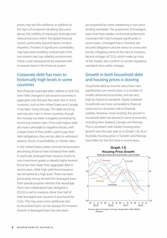
Growth in both household debt and housing prices is slowingHousehold debt-to-income ratios have risen significantly over recent years in a number of smaller advanced economies, and are very high by historical standards. Highly indebted households are more vulnerable to financial stress and so can pose a risk to financial stability. However, more recently, the growth in household debt has slowed in some economies, including New Zealand, Canada, and Norway. This is consistent with slower housing price growth over the past year or so (Graph 1.6). As in Australia, housing prices in Sweden and Norway have fallen for the first time in recent years,
M M M MJ J J JS S S SD D D D2016 2017 20182015
-10
0
10
%
-10
0
10
%
Housing Price GrowthSelected advanced economies, year-ended
Australia
Sweden
Norway
Canada
NZ
Sources: Bank of Canada; CoreLogic; Norges Bank; RBA; REINZ;Riksbank
Graph 1.6
F I N A N C I A L S TA B I L I T Y R E V I E W | O C TO B E R 2018 9
attributed in part to macroprudential policies designed to limit higher-risk lending. To date, these price falls have been orderly and imply an easing in longer-term risks.
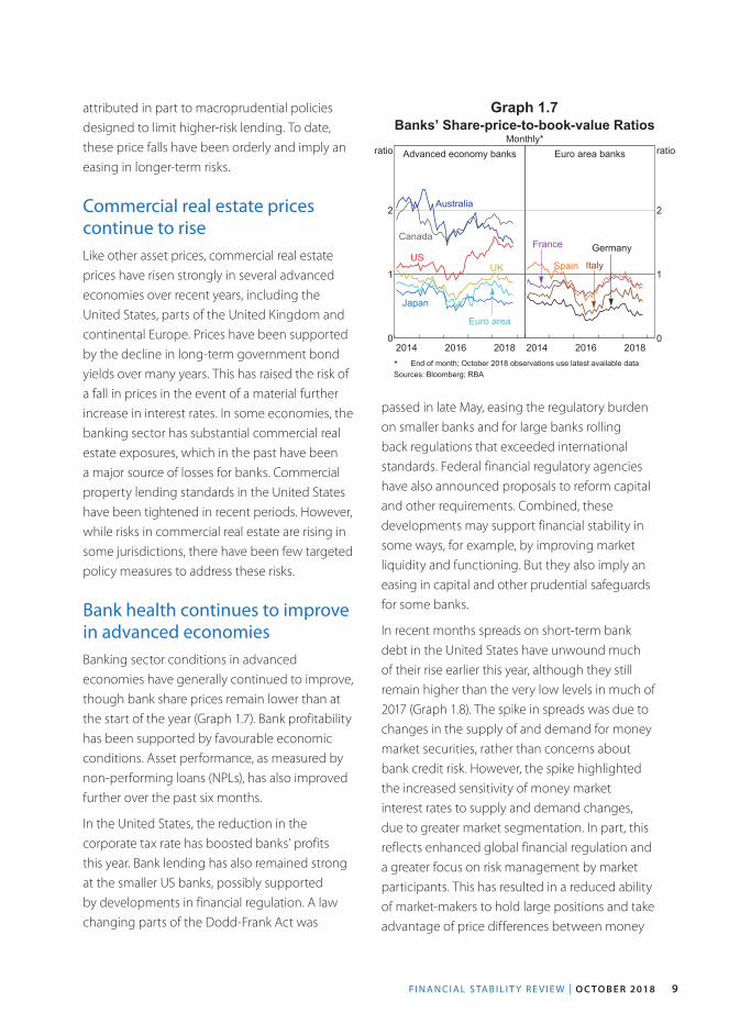
Commercial real estate prices continue to riseLike other asset prices, commercial real estate prices have risen strongly in several advanced economies over recent years, including the United States, parts of the United Kingdom and continental Europe. Prices have been supported by the decline in long-term government bond yields over many years. This has raised the risk of a fall in prices in the event of a material further increase in interest rates. In some economies, the banking sector has substantial commercial real estate exposures, which in the past have been a major source of losses for banks. Commercial property lending standards in the United States have been tightened in recent periods. However, while risks in commercial real estate are rising in some jurisdictions, there have been few targeted policy measures to address these risks.
Bank health continues to improve in advanced economiesBanking sector conditions in advanced economies have generally continued to improve, though bank share prices remain lower than at the start of the year (Graph 1.7). Bank profitability has been supported by favourable economic conditions. Asset performance, as measured by non-performing loans (NPLs), has also improved further over the past six months.
In the United States, the reduction in the corporate tax rate has boosted banks’ profits this year. Bank lending has also remained strong at the smaller US banks, possibly supported by developments in financial regulation. A law changing parts of the Dodd-Frank Act was
passed in late May, easing the regulatory burden on smaller banks and for large banks rolling back regulations that exceeded international standards. Federal financial regulatory agencies have also announced proposals to reform capital and other requirements. Combined, these developments may support financial stability in some ways, for example, by improving market liquidity and functioning. But they also imply an easing in capital and other prudential safeguards for some banks.
In recent months spreads on short-term bank debt in the United States have unwound much of their rise earlier this year, although they still remain higher than the very low levels in much of 2017 (Graph 1.8). The spike in spreads was due to changes in the supply of and demand for money market securities, rather than concerns about bank credit risk. However, the spike highlighted the increased sensitivity of money market interest rates to supply and demand changes, due to greater market segmentation. In part, this reflects enhanced global financial regulation and a greater focus on risk management by market participants. This has resulted in a reduced ability of market-makers to hold large positions and take advantage of price differences between money
Banks’ Share-price-to-book-value RatiosMonthly*
Advanced economy banks
20162014 20180
1
2
ratio
USUK
Canada
Australia
Japan
Euro area
Euro area banks
20162014 20180
1
2
ratio
France Germany
ItalySpain
* End of month; October 2018 observations use latest available dataSources: Bloomberg; RBA
Graph 1.7
R E S E R V E B A N K O F AU S T R A L I A1 0
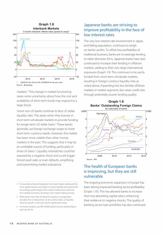
markets.4 This change in market functioning raises some uncertainty about how the cost and availability of short-term funds may respond to a large shock.
Some non-US banks continue to face US dollar liquidity risks. This arises when they borrow in short-term wholesale markets to provide funding for longer-term US dollar loans.5 These banks generally use foreign exchange swaps to meet short-term currency needs. However, this market has been more volatile than other money markets in the past. This suggests that it may be an unreliable source of funding, particularly in times of stress.6 Liquidity mismatches could be exposed by a negative shock and could trigger forced asset sales or even defaults, amplifying and transmitting market turbulence.
4 For example, enhanced regulation has made market-making activity more capital intensive and subject to stricter liquidity risk requirements. Accordingly, profit margins from market-making have declined from already low levels, resulting in less market-making activity.
5 While banks may meet the Basel III Liquidity Coverage Ratio standard, this is measured on an all-currency basis, so liquidity ratios for specific currencies may be significantly lower.
6 For further analysis, see IMF (2018) Global Financial Stability Report, April, pp 38–46.
201620142012 2018-25
0
25
50
75
100
bps
-25
0
25
50
75
100
bps
Interbank Markets3-month interbank offered rates spread to swap*
Euro area
US
UK
* LIBOR for the US and UK; EURIBOR for the euro areaSource: Bloomberg
201420102006 20180
1
2
3
4
US$tr
0
1
2
3
4
US$tr
Banks’ Outstanding Foreign ClaimsBy nationality of banks
GermanyJapanUK
Australia
CanadaUS
France
Source: BIS
Graph 1.8
Graph 1.9
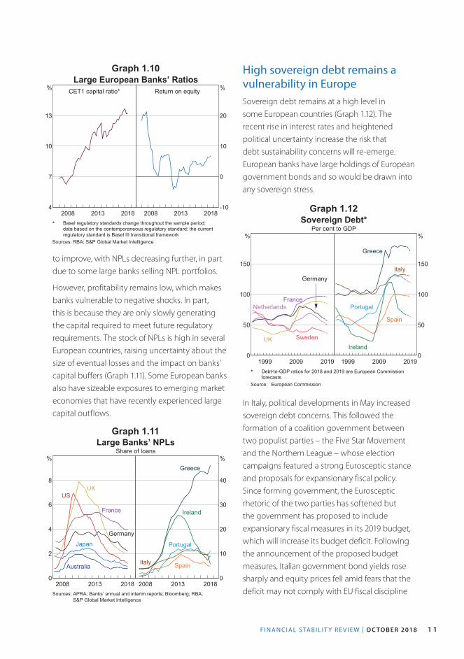
The health of European banks is improving, but they are still vulnerable The ongoing economic expansion in Europe has been driving improved banking sector profitability (Graph 1.10). This has allowed banks to increase their loss-absorbing capital ratios, enhancing their resilience to negative shocks. The quality of banking sector loan portfolios has also continued
Japanese banks are striving to improve profitability in the face of low interest ratesThe very low interest rate environment in Japan, and falling population, continues to weigh on banks’ profits. To offset low profitability of traditional business, banks are increasingly lending to riskier domestic firms. Japanese banks have also continued to increase their lending in offshore markets, adding to their very large international exposures (Graph 1.9). This continues to be partly funded from short-term wholesale markets, resulting in foreign currency liquidity risks as noted above. Expanding into less familiar offshore markets or market segments also raises credit risks through potentially poorer lending quality.
F I N A N C I A L S TA B I L I T Y R E V I E W | O C TO B E R 2018 1 1
Large European Banks’ RatiosCET1 capital ratio*
20132008 20184
7
10
13
% Return on equity
20132008 2018-10
0
10
20
%
* Basel regulatory standards change throughout the sample period;data based on the contemporaneous regulatory standard; the currentregulatory standard is Basel III transitional framework
Sources: RBA; S&P Global Market Intelligence
Large Banks’ NPLsShare of loans
20132008 20180
2
4
6
8
%
Australia
Japan
Germany
France
USUK
20132008 20180
10
20
30
40
%Greece
Portugal
Italy Spain
Ireland
Sources: APRA; Banks’ annual and interim reports; Bloomberg; RBA;S&P Global Market Intelligence
Sovereign Debt*Per cent to GDP
20091999 20190
50
100
150
%
Germany
FranceNetherlands
SwedenUK
20091999 20190
50
100
150
%
Ireland
Italy
Spain
Portugal
Greece
* Debt-to-GDP ratios for 2018 and 2019 are European Commissionforecasts
Source: European Commission
Graph 1.10
Graph 1.11
Graph 1.12
High sovereign debt remains a vulnerability in EuropeSovereign debt remains at a high level in some European countries (Graph 1.12). The recent rise in interest rates and heightened political uncertainty increase the risk that debt sustainability concerns will re-emerge. European banks have large holdings of European government bonds and so would be drawn into any sovereign stress.
to improve, with NPLs decreasing further, in part due to some large banks selling NPL portfolios.
However, profitability remains low, which makes banks vulnerable to negative shocks. In part, this is because they are only slowly generating the capital required to meet future regulatory requirements. The stock of NPLs is high in several European countries, raising uncertainty about the size of eventual losses and the impact on banks’ capital buffers (Graph 1.11). Some European banks also have sizeable exposures to emerging market economies that have recently experienced large capital outflows.
In Italy, political developments in May increased sovereign debt concerns. This followed the formation of a coalition government between two populist parties – the Five Star Movement and the Northern League – whose election campaigns featured a strong Eurosceptic stance and proposals for expansionary fiscal policy. Since forming government, the Eurosceptic rhetoric of the two parties has softened but the government has proposed to include expansionary fiscal measures in its 2019 budget, which will increase its budget deficit. Following the announcement of the proposed budget measures, Italian government bond yields rose sharply and equity prices fell amid fears that the deficit may not comply with EU fiscal discipline
R E S E R V E B A N K O F AU S T R A L I A1 2
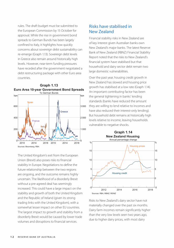
rules. The draft budget must be submitted to the European Commission by 15 October for approval. While the rise in government bond spreads to German Bunds has been largely confined to Italy, it highlights how quickly concerns about sovereign debt sustainability can re-emerge (Graph 1.13). Sovereign debt levels in Greece also remain around historically high levels. However, near-term funding pressures have receded after the government negotiated a debt restructuring package with other Euro area countries.
Risks have stabilised in New Zealand Financial stability risks in New Zealand are of key interest given Australian banks own New Zealand’s major banks. The latest Reserve Bank of New Zealand (RBNZ) Financial Stability Report noted that the risks to New Zealand’s financial system have stabilised but that household and dairy sector debt remain two large domestic vulnerabilities.
Over the past year, housing credit growth in New Zealand has slowed and housing price growth has stabilised at a low rate (Graph 1.14). An important contributing factor has been the general tightening in banks’ lending standards (banks have reduced the amount they are willing to lend relative to incomes and have also reduced their interest-only lending). But household debt remains at historically high levels relative to income, leaving households vulnerable to negative shocks.
Euro Area 10-year Government Bond SpreadsTo German Bunds
20142010 20180
200
400
600
bps
France
Spain
Italy
20142010 20180
1 000
2 000
3 000
bps
Portugal
Greece
Sources: Bloomberg; RBA
Graph 1.13
201620142012 2018-5
0
5
10
15
%
-5
0
5
10
15
%
New Zealand HousingAnnual percentage change
Housing prices
Housing credit
Sources: RBA; RBNZ; REINZ
Graph 1.14
The United Kingdom’s exit from the European Union (Brexit) also poses risks to financial stability in Europe. Negotiations to define the future relationship between the two regions are ongoing, and the outcome remains highly uncertain. The likelihood of a disorderly Brexit without a pre-agreed deal has seemingly increased. This could have a large impact on the stability and growth of both the United Kingdom and the Republic of Ireland (given its strong trading links with the United Kingdom), with a somewhat lesser impact on other EU countries. The largest impact to growth and stability from a disorderly Brexit would be caused by lower trade volumes and disruptions to financial services.
Risks to New Zealand’s dairy sector have not materially changed over the past six months. Dairy farm incomes remain significantly higher than the very low levels seen two years ago, due to higher dairy prices, with most dairy
F I N A N C I A L S TA B I L I T Y R E V I E W | O C TO B E R 2018 1 3
farms currently profitable. The stock of debt has stabilised, but it remains historically high relative to income. Debt is concentrated among more highly leveraged dairy farms, and these farms remain vulnerable to negative shocks, such as a fall in sometimes volatile dairy prices.
In light of reviews in Australia, the RBNZ, together with the New Zealand Financial Markets Authority, is conducting a review into the Australian banks’ New Zealand subsidiaries to assess whether conduct and culture problems are present. The results of the review are expected to be released by November.
Chinese authorities continue to address financial stability risksSince the last Review, Chinese authorities have continued with their efforts to address financial stability risks. A wide range of reforms and policy actions have been implemented or proposed (see ‘Box A: Ongoing Financial Regulatory Reform in China’). The authorities have focused on measures to tackle high debt levels and to reduce risks related to non-bank financial institutions’ (NBFIs) activities. These reforms are helping to contain the build-up of financial stability risks in China.
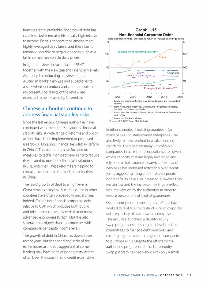
The rapid growth of debt to a high level in China remains a key risk. Such build-ups in other countries have often preceded financial crises. Indeed, China’s non-financial corporate debt relative to GDP, which includes both public and private enterprises, exceeds that of most advanced economies (Graph 1.15). It is also several times higher than in economies with comparable per capita income levels.
The growth of debt in China has slowed over recent years. But the speed and scale of the earlier increase in debt suggests that some lending may have been of poor quality, as has often been the case in rapid credit expansions
2015201220092006 20180
50
100
150
%
0
50
100
150
%
Non-financial Corporate Debt*Selected economies, per cent to GDP at market exchange rates
China
Advanced
Emerging Latin America****
Asia**(excl. China and Japan)
Selected other emerging markets***
* Loans and other debt funding provided by domestic and non-residentsources** Hong Kong, India, Indonesia, Malaysia, the Philippines, Singapore,South Korea, Taiwan and Thailand*** Czech Republic, Hungary, Poland, Russia, Saudi Arabia, South Africaand Turkey**** Argentina, Brazil and Mexico
Sources: BIS; CEIC Data; RBA; Refinitiv
Graph 1.15
in other countries. Implicit guarantees – for many banks and state-owned enterprises – are also likely to have resulted in weaker lending standards. There remain many unprofitable companies in parts of the industrial sector, given excess capacity, that are highly leveraged and rely on loan forbearance to survive. The flow of new NPLs has increased noticeably over recent years, suggesting rising credit risks. Corporate bond defaults have also increased. However, they remain low and the increase may largely reflect less intervention by the authorities in order to reduce perceptions of implicit guarantees.
Over recent years, the authorities in China have worked to facilitate the restructuring of corporate debt, especially of state-owned enterprises. This includes launching a debt-to-equity swap program, establishing firm-level creditor committees to manage debt workouts, and creating regional asset management companies to purchase NPLs. Despite the efforts by the authorities, progress on the debt-to-equity swap program has been slow, with only a small
R E S E R V E B A N K O F AU S T R A L I A1 4
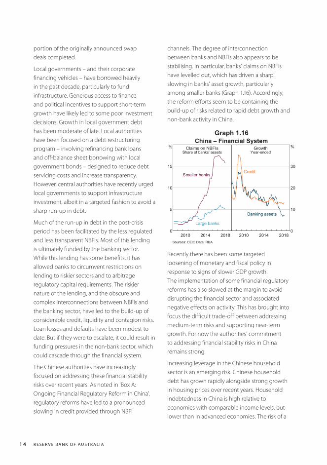
channels. The degree of interconnection between banks and NBFIs also appears to be stabilising. In particular, banks’ claims on NBFIs have levelled out, which has driven a sharp slowing in banks’ asset growth, particularly among smaller banks (Graph 1.16). Accordingly, the reform efforts seem to be containing the build-up of risks related to rapid debt growth and non-bank activity in China.
portion of the originally announced swap deals completed.
Local governments – and their corporate financing vehicles – have borrowed heavily in the past decade, particularly to fund infrastructure. Generous access to finance and political incentives to support short-term growth have likely led to some poor investment decisions. Growth in local government debt has been moderate of late. Local authorities have been focused on a debt restructuring program – involving refinancing bank loans and off-balance sheet borrowing with local government bonds – designed to reduce debt servicing costs and increase transparency. However, central authorities have recently urged local governments to support infrastructure investment, albeit in a targeted fashion to avoid a sharp run-up in debt.
Much of the run-up in debt in the post-crisis period has been facilitated by the less regulated and less transparent NBFIs. Most of this lending is ultimately funded by the banking sector. While this lending has some benefits, it has allowed banks to circumvent restrictions on lending to riskier sectors and to arbitrage regulatory capital requirements. The riskier nature of the lending, and the obscure and complex interconnections between NBFIs and the banking sector, have led to the build-up of considerable credit, liquidity and contagion risks. Loan losses and defaults have been modest to date. But if they were to escalate, it could result in funding pressures in the non-bank sector, which could cascade through the financial system.
The Chinese authorities have increasingly focused on addressing these financial stability risks over recent years. As noted in ‘Box A: Ongoing Financial Regulatory Reform in China’, regulatory reforms have led to a pronounced slowing in credit provided through NBFI
China – Financial SystemClaims on NBFIs
Share of banks’ assets
20142010 20180
5
10
15
%
Large banks
Smaller banks
GrowthYear-ended
20142010 20180
10
20
30
%
Banking assets
Credit
Sources: CEIC Data; RBA
Graph 1.16
Recently there has been some targeted loosening of monetary and fiscal policy in response to signs of slower GDP growth. The implementation of some financial regulatory reforms has also slowed at the margin to avoid disrupting the financial sector and associated negative effects on activity. This has brought into focus the difficult trade-off between addressing medium-term risks and supporting near-term growth. For now the authorities’ commitment to addressing financial stability risks in China remains strong.
Increasing leverage in the Chinese household sector is an emerging risk. Chinese household debt has grown rapidly alongside strong growth in housing prices over recent years. Household indebtedness in China is high relative to economies with comparable income levels, but lower than in advanced economies. The risk of a
F I N A N C I A L S TA B I L I T Y R E V I E W | O C TO B E R 2018 1 5
sharp decline in housing prices, which would also negatively affect property developers and local governments, is mitigated by the authorities’ active management of the housing market using a variety of tools.
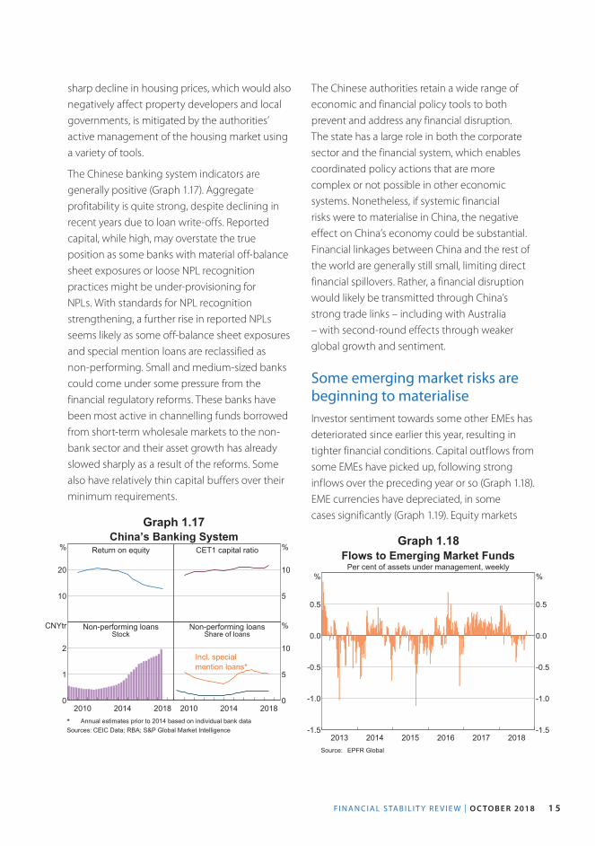
The Chinese banking system indicators are generally positive (Graph 1.17). Aggregate profitability is quite strong, despite declining in recent years due to loan write-offs. Reported capital, while high, may overstate the true position as some banks with material off-balance sheet exposures or loose NPL recognition practices might be under-provisioning for NPLs. With standards for NPL recognition strengthening, a further rise in reported NPLs seems likely as some off-balance sheet exposures and special mention loans are reclassified as non-performing. Small and medium-sized banks could come under some pressure from the financial regulatory reforms. These banks have been most active in channelling funds borrowed from short-term wholesale markets to the non-bank sector and their asset growth has already slowed sharply as a result of the reforms. Some also have relatively thin capital buffers over their minimum requirements.
The Chinese authorities retain a wide range of economic and financial policy tools to both prevent and address any financial disruption. The state has a large role in both the corporate sector and the financial system, which enables coordinated policy actions that are more complex or not possible in other economic systems. Nonetheless, if systemic financial risks were to materialise in China, the negative effect on China’s economy could be substantial. Financial linkages between China and the rest of the world are generally still small, limiting direct financial spillovers. Rather, a financial disruption would likely be transmitted through China’s strong trade links – including with Australia – with second-round effects through weaker global growth and sentiment.
Some emerging market risks are beginning to materialiseInvestor sentiment towards some other EMEs has deteriorated since earlier this year, resulting in tighter financial conditions. Capital outflows from some EMEs have picked up, following strong inflows over the preceding year or so (Graph 1.18). EME currencies have depreciated, in some cases significantly (Graph 1.19). Equity markets
China’s Banking SystemReturn on equity
10
20
% CET1 capital ratio
5
10
%
Non-performing loansStock
20142010 20180
1
2
CNYtr Non-performing loansShare of loans
20142010 20180
5
10
%
Incl. specialmention loans*
* Annual estimates prior to 2014 based on individual bank dataSources: CEIC Data; RBA; S&P Global Market Intelligence
Graph 1.17
20172016201520142013 2018-1.5
-1.0
-0.5
0.0
0.5
%
-1.5
-1.0
-0.5
0.0
0.5
%
Flows to Emerging Market FundsPer cent of assets under management, weekly
Source: EPFR Global
Graph 1.18
R E S E R V E B A N K O F AU S T R A L I A1 6
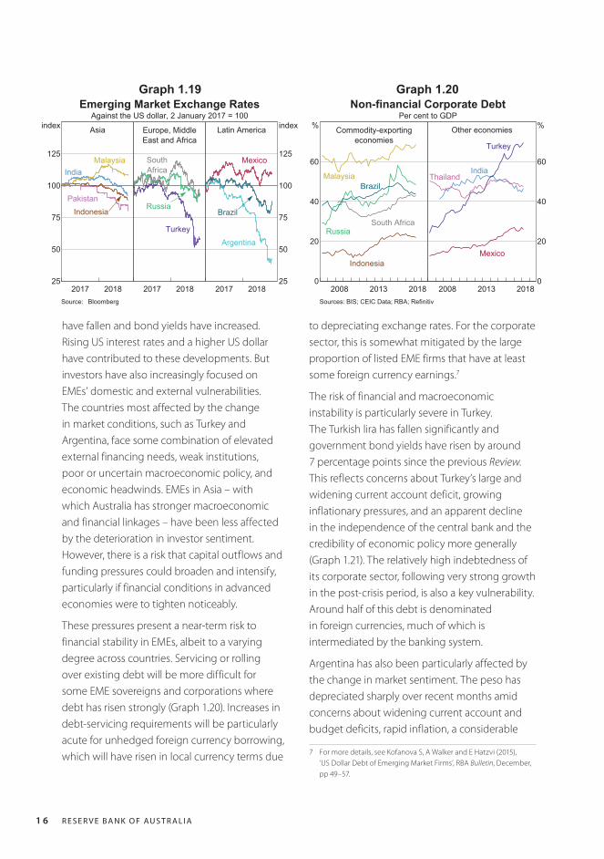
have fallen and bond yields have increased. Rising US interest rates and a higher US dollar have contributed to these developments. But investors have also increasingly focused on EMEs’ domestic and external vulnerabilities. The countries most affected by the change in market conditions, such as Turkey and Argentina, face some combination of elevated external financing needs, weak institutions, poor or uncertain macroeconomic policy, and economic headwinds. EMEs in Asia – with which Australia has stronger macroeconomic and financial linkages – have been less affected by the deterioration in investor sentiment. However, there is a risk that capital outflows and funding pressures could broaden and intensify, particularly if financial conditions in advanced economies were to tighten noticeably.
These pressures present a near-term risk to financial stability in EMEs, albeit to a varying degree across countries. Servicing or rolling over existing debt will be more difficult for some EME sovereigns and corporations where debt has risen strongly (Graph 1.20). Increases in debt-servicing requirements will be particularly acute for unhedged foreign currency borrowing, which will have risen in local currency terms due
to depreciating exchange rates. For the corporate sector, this is somewhat mitigated by the large proportion of listed EME firms that have at least some foreign currency earnings.7
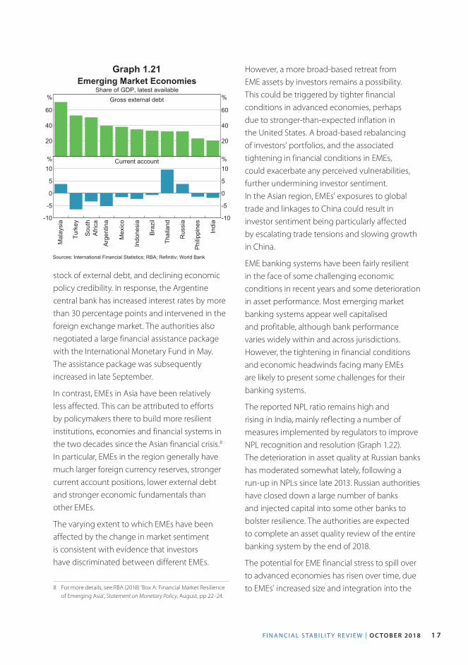
The risk of financial and macroeconomic instability is particularly severe in Turkey. The Turkish lira has fallen significantly and government bond yields have risen by around 7 percentage points since the previous Review. This reflects concerns about Turkey’s large and widening current account deficit, growing inflationary pressures, and an apparent decline in the independence of the central bank and the credibility of economic policy more generally (Graph 1.21). The relatively high indebtedness of its corporate sector, following very strong growth in the post-crisis period, is also a key vulnerability. Around half of this debt is denominated in foreign currencies, much of which is intermediated by the banking system.
Argentina has also been particularly affected by the change in market sentiment. The peso has depreciated sharply over recent months amid concerns about widening current account and budget deficits, rapid inflation, a considerable
7 For more details, see Kofanova S, A Walker and E Hatzvi (2015), ‘US Dollar Debt of Emerging Market Firms’, RBA Bulletin, December, pp 49–57.
Emerging Market Exchange RatesAgainst the US dollar, 2 January 2017 = 100
Asia
2017 201825
50
75
100
125
index
MalaysiaIndia
PakistanIndonesia
Europe, MiddleEast and Africa
2017 2018
Turkey
Russia
SouthAfrica
Latin America
2017 201825
50
75
100
125
index
Argentina
Brazil
Mexico
Source: Bloomberg
Non-financial Corporate DebtPer cent to GDP
Commodity-exportingeconomies
20132008 20180
20
40
60
%
Russia
Brazil
South Africa
Indonesia
Malaysia
Other economies
20132008 20180
20
40
60
%
Turkey
India
Mexico
Thailand
Sources: BIS; CEIC Data; RBA; Refinitiv
Graph 1.19 Graph 1.20
F I N A N C I A L S TA B I L I T Y R E V I E W | O C TO B E R 2018 1 7
stock of external debt, and declining economic policy credibility. In response, the Argentine central bank has increased interest rates by more than 30 percentage points and intervened in the foreign exchange market. The authorities also negotiated a large financial assistance package with the International Monetary Fund in May. The assistance package was subsequently increased in late September.
In contrast, EMEs in Asia have been relatively less affected. This can be attributed to efforts by policymakers there to build more resilient institutions, economies and financial systems in the two decades since the Asian financial crisis.8 In particular, EMEs in the region generally have much larger foreign currency reserves, stronger current account positions, lower external debt and stronger economic fundamentals than other EMEs.
The varying extent to which EMEs have been affected by the change in market sentiment is consistent with evidence that investors have discriminated between different EMEs.
8 For more details, see RBA (2018) ‘Box A: Financial Market Resilience of Emerging Asia’, Statement on Monetary Policy, August, pp 22–24.
However, a more broad-based retreat from EME assets by investors remains a possibility. This could be triggered by tighter financial conditions in advanced economies, perhaps due to stronger-than-expected inflation in the United States. A broad-based rebalancing of investors’ portfolios, and the associated tightening in financial conditions in EMEs, could exacerbate any perceived vulnerabilities, further undermining investor sentiment. In the Asian region, EMEs’ exposures to global trade and linkages to China could result in investor sentiment being particularly affected by escalating trade tensions and slowing growth in China.
EME banking systems have been fairly resilient in the face of some challenging economic conditions in recent years and some deterioration in asset performance. Most emerging market banking systems appear well capitalised and profitable, although bank performance varies widely within and across jurisdictions. However, the tightening in financial conditions and economic headwinds facing many EMEs are likely to present some challenges for their banking systems.
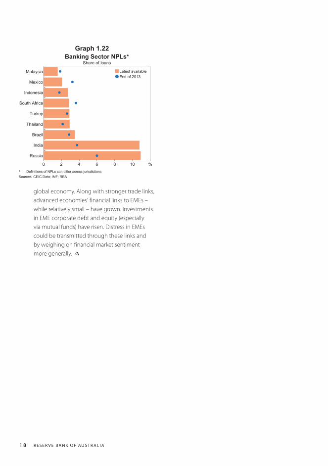
The reported NPL ratio remains high and rising in India, mainly reflecting a number of measures implemented by regulators to improve NPL recognition and resolution (Graph 1.22). The deterioration in asset quality at Russian banks has moderated somewhat lately, following a run-up in NPLs since late 2013. Russian authorities have closed down a large number of banks and injected capital into some other banks to bolster resilience. The authorities are expected to complete an asset quality review of the entire banking system by the end of 2018.
The potential for EME financial stress to spill over to advanced economies has risen over time, due to EMEs’ increased size and integration into the
Emerging Market EconomiesShare of GDP, latest available
Gross external debt
20
40
60
%
20
40
60
%
Current account
Mal
aysi
a
Turk
ey
Sou
thA
frica
Arg
entin
a
Mex
ico
Indo
nesi
a
Bra
zil
Thai
land
Rus
sia
Phi
lippi
nes
Indi
a-10
-5
0
5
10%
-10
-5
0
5
10%
Sources: International Financial Statistics; RBA; Refinitiv; World Bank
Graph 1.21
R E S E R V E B A N K O F AU S T R A L I A1 8
global economy. Along with stronger trade links, advanced economies’ financial links to EMEs – while relatively small – have grown. Investments in EME corporate debt and equity (especially via mutual funds) have risen. Distress in EMEs could be transmitted through these links and by weighing on financial market sentiment more generally. R
Latest availableEnd of 2013
0 2 4 6 8 10 %
Russia
India
Brazil
Thailand
Turkey
South Africa
Indonesia
Mexico
Malaysia
Banking Sector NPLs*Share of loans
* Definitions of NPLs can differ across jurisdictionsSources: CEIC Data; IMF; RBA
Graph 1.22
F I N A N C I A L S TA B I L I T Y R E V I E W | O C TO B E R 2018 19
Box A
Ongoing Financial Regulatory Reform in China
Financial stability risks remain a key focus for the authorities in China. President Xi Jinping has characterised the management of financial stability risks as a national security issue. To address the build-up of risks, the Chinese authorities have announced a series of reforms in recent years. These have focused on reducing indirect lending undertaken through the non-bank sector, simplifying complex interconnections within the financial system, reducing high levels of corporate leverage, and improving banking system resilience. This box focuses on the reforms undertaken over the past year. It discusses the effect of reforms to date on lending and considers some implications for growth. Over the past year: regulatory oversight has been consolidated; existing regulations have been enhanced and more strictly enforced; and sweeping asset management sector reforms have been finalised. Several indicators suggest that the reforms are gaining traction; for example, measures of non-bank lending growth have slowed. However, the regulatory tightening appears to be resulting in tighter financing conditions for businesses and is weighing on growth in parts of the economy.
Reforms up to mid 2017 focused on lending through the non-bank sectorRegulatory reform to address financial stability risks has been an ongoing process that started in earnest several years ago.1 Reforms in recent
1 For a more extensive discussion of the reforms up to mid 2017, see RBA (2017), ‘Box B: Recent Developments in Chinese Financial Regulations,’ Statement on Monetary Policy, August, pp 27–29.
years focused on reducing ‘channel lending’. Channel lending is where banks lend or invest using non-bank financial institutions (NBFIs) to intermediate between the bank and the borrower. Banks typically fund this lending using short-term funds raised from other banks or retail investors. This form of regulatory arbitrage has raised significant credit, liquidity and contagion risks. Reforms in recent years have included: measures to reduce banks’ ability and incentive to engage in channel lending; proposals to improve the transparency and risk management of asset management products (AMPs) issued and used by banks and NBFIs to facilitate channel lending; and restrictions on short-term interbank lending and borrowing. These reforms were complemented by the People’s Bank of China (PBC) revising its macroprudential assessment (MPA) program to include off-balance sheet assets, such as AMPs, in banks’ prudential assessments.
Regulation has tightened further since 2017, especially for the asset management sectorOver the past year, authorities have more strictly enforced existing regulation and finalised additional reforms that focused on: consolidating regulatory oversight; further reducing channel lending by implementing the asset management reforms; and increasing resilience in the banking sector. The consolidation of regulatory oversight should reduce regulatory arbitrage (by revealing regulatory gaps and fostering similar regulation of similar activities). A new Financial Stability
R E S E R V E B A N K O F AU S T R A L I A20
and Development Committee, chaired by a Vice Premier, was established under the State Council. This committee aims to boost coordination between the main Chinese financial regulators and increase their authority. The banking and insurance regulators were also merged to form the China Banking and Insurance Regulatory Commission (CBIRC). At the same time, the role of the PBC was expanded to give it greater influence in the setting of financial regulatory policy. The State Council has also suggested that it will build a national database to consolidate and expand the collection of data on the entire financial system. This would improve regulators’ visibility of financial stability risks and the effects of reforms.
At the start of 2018, the PBC began phasing in the asset management sector reforms that were foreshadowed in the previous year. The regulations seek to address a range of risks related to non-bank financial intermediation, including regulatory arbitrage, implicit guarantees, interconnectedness and liquidity risks. The rules focus on AMPs, which refer to a broad range of financial products that offer the holder the right to the income stream from underlying assets (which can include loans as well as other financial assets). There are often complex layers of cross-investment between AMPs, which makes it difficult to see the ultimate exposures. The new measures aim to reduce contagion risks by reducing complex interconnections between financial products. They prohibit cross-investment by banks and asset managers in one another’s AMPs.
To address credit and liquidity risks, the new regulations place restrictions on the extent to which AMPs can invest in non-standardised debt assets (NSDAs). NSDA is a term used by Chinese financial regulators to describe debt assets that are not traded in a liquid market. This includes trust loans, entrusted loans and bank-accepted
bills.2 To address regulatory arbitrage, issuers of AMPs that are allowed to invest in NSDAs will be subject to capital and liquidity requirements. Since NSDAs are key assets used for channel lending, these changes will reduce banks’ ability and incentive to engage in such lending.
The asset management reforms also address explicit guarantees, which can result in risky lending practices and contingent liabilities for financial institutions. Under the new rules, AMP issuers are prohibited from providing principal and income guarantees and will need to frequently report a floating Net Asset Value to investors. The rules also prohibit borrowing to invest in AMPs. AMPs had been used to circumvent regulations on leveraged investing. Together, these measures should discourage risky lending and investing practices.
Despite the extensive reforms, financial innovation to circumvent regulation continues. For example, as regulations targeting AMPs were tightened, banks increased their use of ‘structured deposits’ to boost funding. These are on-balance sheet investment products with a principal guarantee, and investment returns linked to asset prices through derivatives exposure. In response, the CBIRC released guidance requiring banks offering structured deposits to be qualified to engage in derivatives transactions. This burden is prohibitive for many small and medium-sized banks, and has resulted in a decline in the issuance of structured deposits. However, the
2 Trust companies make investments (including writing loans) and manage assets on behalf of clients, and are the largest type of NBFI in China. Entrusted loans are inter-company loans facilitated by a financial institution. Bank-accepted bills are short-term tradeable debt instruments used by banks and companies to lend to other companies. Other types of NSDAs include: letters of credit; accounts receivable; securitised bank loans or other non-standard forms of debt. For more details on non-bank financing in China, see Bowman J, M Hack and M Waring (2018), ‘Non-bank Financing in China’, RBA Bulletin, March, viewed 9 October 2018. Available at <https://www.rba.gov.au/publications/bulletin/2018/mar/non-bank-financing-in-china.html>.
F I N A N C I A L S TA B I L I T Y R E V I E W | O C TO B E R 2018 21
Graph A2
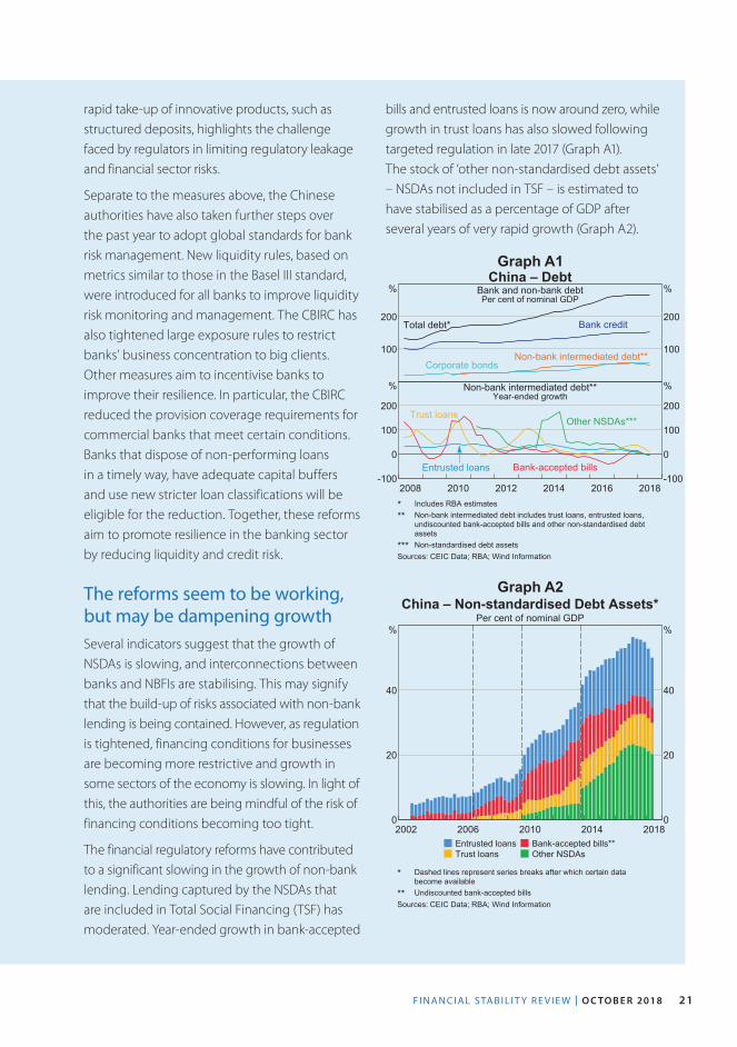
rapid take-up of innovative products, such as structured deposits, highlights the challenge faced by regulators in limiting regulatory leakage and financial sector risks.
Separate to the measures above, the Chinese authorities have also taken further steps over the past year to adopt global standards for bank risk management. New liquidity rules, based on metrics similar to those in the Basel III standard, were introduced for all banks to improve liquidity risk monitoring and management. The CBIRC has also tightened large exposure rules to restrict banks’ business concentration to big clients. Other measures aim to incentivise banks to improve their resilience. In particular, the CBIRC reduced the provision coverage requirements for commercial banks that meet certain conditions. Banks that dispose of non-performing loans in a timely way, have adequate capital buffers and use new stricter loan classifications will be eligible for the reduction. Together, these reforms aim to promote resilience in the banking sector by reducing liquidity and credit risk.
The reforms seem to be working, but may be dampening growthSeveral indicators suggest that the growth of NSDAs is slowing, and interconnections between banks and NBFIs are stabilising. This may signify that the build-up of risks associated with non-bank lending is being contained. However, as regulation is tightened, financing conditions for businesses are becoming more restrictive and growth in some sectors of the economy is slowing. In light of this, the authorities are being mindful of the risk of financing conditions becoming too tight.
The financial regulatory reforms have contributed to a significant slowing in the growth of non-bank lending. Lending captured by the NSDAs that are included in Total Social Financing (TSF) has moderated. Year-ended growth in bank-accepted
Graph A1
bills and entrusted loans is now around zero, while growth in trust loans has also slowed following targeted regulation in late 2017 (Graph A1). The stock of ‘other non-standardised debt assets’ – NSDAs not included in TSF – is estimated to have stabilised as a percentage of GDP after several years of very rapid growth (Graph A2).
2014201020062002 20180
20
40
%
0
20
40
%
China – Non-standardised Debt Assets*Per cent of nominal GDP
Entrusted loansTrust loans
Bank-accepted bills**Other NSDAs
* Dashed lines represent series breaks after which certain databecome available** Undiscounted bank-accepted bills
Sources: CEIC Data; RBA; Wind Information
China – DebtBank and non-bank debtPer cent of nominal GDP
100
200
%
100
200
%
Bank credit
Corporate bonds
Total debt*
Non-bank intermediated debt**
Non-bank intermediated debt**Year-ended growth
20162014201220102008 2018-100
0
100
200
%
-100
0
100
200
%
Entrusted loans
Trust loans
Bank-accepted bills
Other NSDAs***
* Includes RBA estimates** Non-bank intermediated debt includes trust loans, entrusted loans,undiscounted bank-accepted bills and other non-standardised debtassets*** Non-standardised debt assets
Sources: CEIC Data; RBA; Wind Information
R E S E R V E B A N K O F AU S T R A L I A22
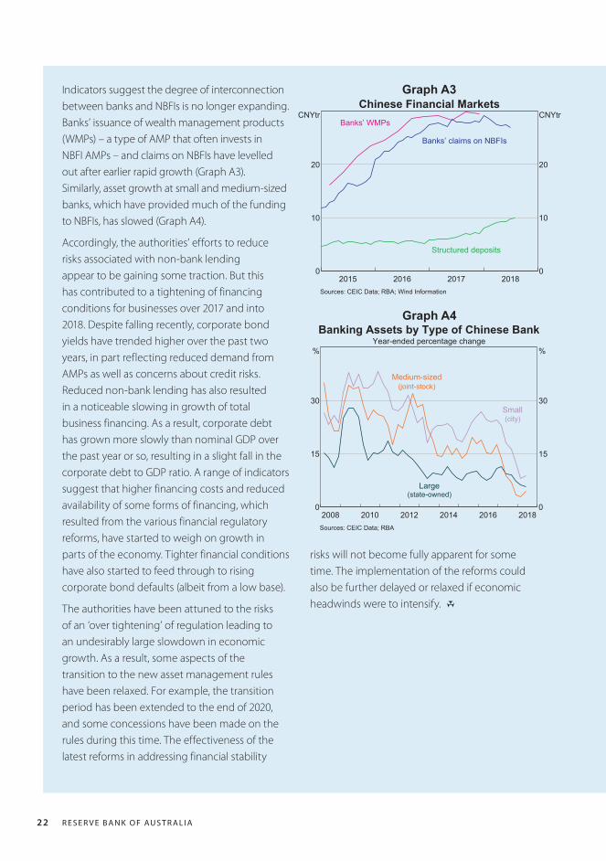
Indicators suggest the degree of interconnection between banks and NBFIs is no longer expanding. Banks’ issuance of wealth management products (WMPs) – a type of AMP that often invests in NBFI AMPs – and claims on NBFIs have levelled out after earlier rapid growth (Graph A3). Similarly, asset growth at small and medium-sized banks, which have provided much of the funding to NBFIs, has slowed (Graph A4).
Accordingly, the authorities’ efforts to reduce risks associated with non-bank lending appear to be gaining some traction. But this has contributed to a tightening of financing conditions for businesses over 2017 and into 2018. Despite falling recently, corporate bond yields have trended higher over the past two years, in part reflecting reduced demand from AMPs as well as concerns about credit risks. Reduced non-bank lending has also resulted in a noticeable slowing in growth of total business financing. As a result, corporate debt has grown more slowly than nominal GDP over the past year or so, resulting in a slight fall in the corporate debt to GDP ratio. A range of indicators suggest that higher financing costs and reduced availability of some forms of financing, which resulted from the various financial regulatory reforms, have started to weigh on growth in parts of the economy. Tighter financial conditions have also started to feed through to rising corporate bond defaults (albeit from a low base).
The authorities have been attuned to the risks of an ‘over tightening’ of regulation leading to an undesirably large slowdown in economic growth. As a result, some aspects of the transition to the new asset management rules have been relaxed. For example, the transition period has been extended to the end of 2020, and some concessions have been made on the rules during this time. The effectiveness of the latest reforms in addressing financial stability
Graph A4
Graph A3
risks will not become fully apparent for some time. The implementation of the reforms could also be further delayed or relaxed if economic headwinds were to intensify. R
201720162015 20180
10
20
CNYtr
0
10
20
CNYtrChinese Financial Markets
Banks’ claims on NBFIs
Banks’ WMPs
Structured deposits
Sources: CEIC Data; RBA; Wind Information
20162014201220102008 20180
15
30
%
0
15
30
%
Banking Assets by Type of Chinese BankYear-ended percentage change
(state-owned)Large
(joint-stock)Medium-sized
Small(city)
Sources: CEIC Data; RBA
F I N A N C I A L S TA B I L I T Y R E V I E W | O C TO B E R 2018 2 3
2. Household and Business Finances
In Australia, financial risks to the household sector remain elevated given the high level of household debt. However, the quality of banks’ housing lending has continued to improve in response to tighter lending standards. This is strengthening the resilience of household and bank balance sheets. The changes to lending standards are affecting the borrowers least able to afford a loan but to date have not had a large impact on the supply of credit to most borrowers. Risks in housing markets are evolving as the sector absorbs the impact of tighter lending standards alongside weaker demand, which has been reflected in slower credit growth. Housing market conditions have eased, particularly in Sydney and Melbourne, with a shift in the underlying supply and demand dynamics playing an important role. The easing in prices is small relative to the very large increase in the preceding years and is taking place within a positive macroeconomic environment. However, this adjustment raises some risks – such as possible negative equity for some very recent purchasers, or a reduction in wealth weighing on consumption. A large or rapid correction in housing prices could be disruptive for the financial system and household balance sheets.
The pace of increase in household indebtedness has slowed. In aggregate, households appear well placed to manage their debt obligations, given currently low interest rates and the improvement in lending standards. However, some households are experiencing financial stress, especially in Western Australia. Most households continue to accumulate prepayments, although at a slower pace than in recent years. Household wealth has fallen a little, mainly due to falls in housing prices.
The risks from residential development have eased. These risks arose from the construction of a large number of new apartments. These new apartments are being purchased with only isolated instances of large falls in valuations at settlement compared with the purchase price. Settlement failures remain low. The stock of apartments under construction is lower than it was a couple of years ago. Apartment market conditions remain challenging in Perth, though the size of the Perth apartment market is small relative to the eastern states.
For non-residential commercial property, valuations continue to rise rapidly in the eastern states and yields have fallen further. There is a risk that if these valuations prove unsustainable then price falls could see highly leveraged investors breach their loan covenants. This could trigger sales and further price falls. The risks appear greatest for retail commercial property owners given challenging trading conditions for their tenants. Foreign banks and non-bank lenders have continued to increase their exposures to commercial property, while the domestic banks’ exposures have remained steady.
The financial health of the business sector is generally good, supported by positive economic conditions and low interest rates. The resources sector’s earnings have increased, consistent with higher commodity prices. However, some sectors are experiencing more difficult conditions. These include the drought-affected agricultural sector in the eastern states, and some bricks-and-mortar retailers in the consumer discretionary sector.
R E S E R V E B A N K O F AU S T R A L I A2 4
Banks have improved the quality of mortgagesImprovements in the quality of banks’ mortgage lending have occurred in response to a range of regulatory measures implemented by the Australian Prudential Regulation Authority (APRA) and the Australian Securities and Investments Commission (ASIC) over recent years (for further detail, see the special chapter, ‘Assessing the Effects of Housing Lending Policy Measures’). Loans with a high loan-to-valuation ratio (LVR), especially those with an LVR exceeding 90 per cent, remain a low share of new lending. The share of new interest-only (IO) lending has fallen sharply to 17 per cent of new loan approvals, well below the regulatory cap. In addition, the stock of IO loans is down by 10 percentage points since June 2017 to just under 30 per cent of outstanding loans. A large number of borrowers have switched their IO loans to principal and interest loans (to avoid the higher interest rates on IO loans).
While the largest changes to lending standards have already occurred, various factors could result in some further adjustments. APRA announced in April 2018 that banks can apply to have the 10 per cent investor lending benchmark lifted subject to meeting certain conditions. Among other things, bank boards will be expected to attest that their lending policies meet APRA’s guidance on serviceability and their lending practices will be strengthened where necessary. Bank boards have also been asked to set limits (not prohibitions) on lending with debt-to-income (DTI) ratios exceeding six. This approach recognises that some high DTI lending meets prudential standards and can be justified on a risk basis. The introduction of comprehensive credit reporting over the next 12 months will improve banks’ ability to know about all the debt obligations of borrowers. ASIC’s recent legal settlement with Westpac on compliance with responsible lending laws may
improve understanding about responsible lending requirements for all housing lenders.
The banks, in conjunction with APRA, have been working to improve how living expenses are estimated in loan applications. Banks are scrutinising expenses more closely and this is leading to some loan approvals taking more time. The Royal Commission into Misconduct in the Banking, Superannuation and Financial Services Industry could prompt further changes to lending practices. The cumulative effect of past, and prospective, changes will be to reduce the maximum loan size available to many households. In practice, however, most households will be relatively unaffected since only a small share borrow close to the maximum amount. The prospective borrowers most affected will be those who are least able to afford the loan and these borrowers account for only a small share of new credit. Overall these changes should improve the resilience of borrowers taking out their maximum loan, without having a material effect on aggregate credit availability and growth (See ‘Box B: The Impact of Lending Standards on Loan Sizes’).
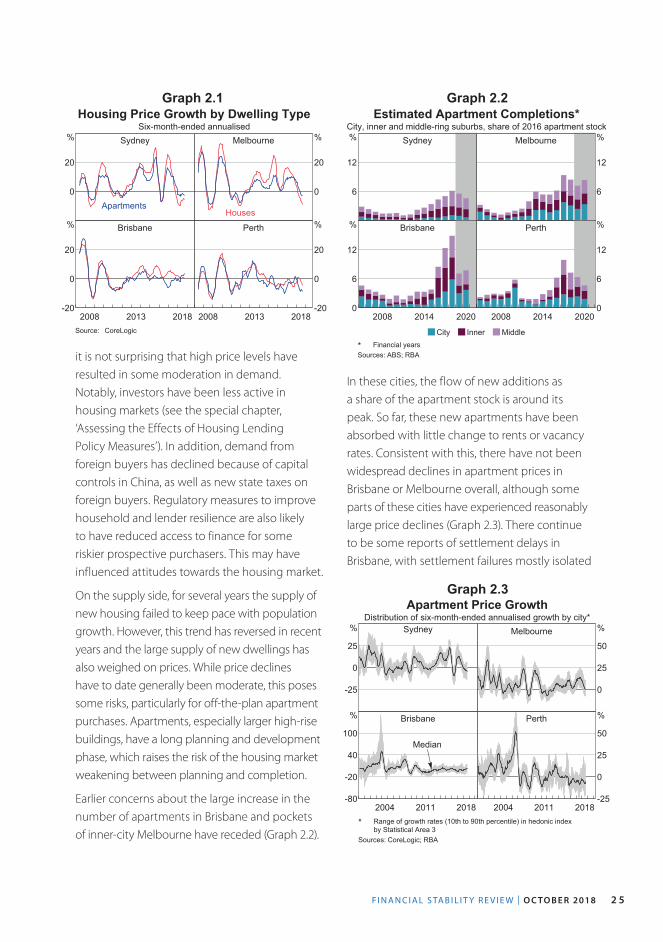
Conditions in housing markets have eased Nationwide, housing prices fell at an annual rate of around 3½ per cent over the six months to September driven mostly by prices in Sydney and Melbourne (Graph 2.1). The largest decline in prices in these cities has been for more expensive properties. Despite the recent price declines, prices in Sydney and Melbourne remain around 50–60 per cent higher than in 2012. In Brisbane, housing prices have been fairly stable over the past year, while conditions in Perth remain weak.
There are a number of demand-side explanations for the recent easing in housing prices. Following the strong price growth between 2012 and 2017,
F I N A N C I A L S TA B I L I T Y R E V I E W | O C TO B E R 2018 2 5
Graph 2.1Housing Price Growth by Dwelling Type
Six-month-ended annualisedSydney
0
20
%
Apartments
Melbourne
0
20
%
Houses
Brisbane
20132008 2018-20
0
20
% Perth
20132008 2018-20
0
20
%
Source: CoreLogic
it is not surprising that high price levels have resulted in some moderation in demand. Notably, investors have been less active in housing markets (see the special chapter, ‘Assessing the Effects of Housing Lending Policy Measures’). In addition, demand from foreign buyers has declined because of capital controls in China, as well as new state taxes on foreign buyers. Regulatory measures to improve household and lender resilience are also likely to have reduced access to finance for some riskier prospective purchasers. This may have influenced attitudes towards the housing market.
On the supply side, for several years the supply of new housing failed to keep pace with population growth. However, this trend has reversed in recent years and the large supply of new dwellings has also weighed on prices. While price declines have to date generally been moderate, this poses some risks, particularly for off-the-plan apartment purchases. Apartments, especially larger high-rise buildings, have a long planning and development phase, which raises the risk of the housing market weakening between planning and completion.
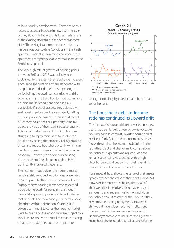
Earlier concerns about the large increase in the number of apartments in Brisbane and pockets of inner-city Melbourne have receded (Graph 2.2).
In these cities, the flow of new additions as a share of the apartment stock is around its peak. So far, these new apartments have been absorbed with little change to rents or vacancy rates. Consistent with this, there have not been widespread declines in apartment prices in Brisbane or Melbourne overall, although some parts of these cities have experienced reasonably large price declines (Graph 2.3). There continue to be some reports of settlement delays in Brisbane, with settlement failures mostly isolated
Graph 2.2Estimated Apartment Completions*
City, inner and middle-ring suburbs, share of 2016 apartment stockSydney
6
12
% Melbourne
6
12
%
Brisbane
20142008 20200
6
12
% Perth
20142008 20200
6
12
%
City Inner Middle* Financial yearsSources: ABS; RBA
Graph 2.3Apartment Price Growth
Distribution of six-month-ended annualised growth by city*Sydney
-25
0
25
% Melbourne
0
25
50
%
Brisbane
20112004 2018-80
-20
40
100
%
Median
Perth
20112004 2018-25
0
25
50
%
* Range of growth rates (10th to 90th percentile) in hedonic indexby Statistical Area 3
Sources: CoreLogic; RBA
R E S E R V E B A N K O F AU S T R A L I A2 6
to lower-quality developments. There has been a recent substantial increase in new apartments in Sydney although this accounts for a smaller share of the existing stock than in the other east coast cities. The easing in apartment prices in Sydney has been gradual to date. Conditions in the Perth apartment market remain more challenging, but apartments comprise a relatively small share of the Perth housing stock.
The very high rate of growth of housing prices between 2012 and 2017 was unlikely to be sustained. To the extent that rapid price increases encourage speculation and are associated with rising household indebtedness, a prolonged period of rapid growth can contribute to risks accumulating. The transition to more sustainable housing market conditions also has risks, particularly if a shock accentuates a slowdown and housing prices decline very rapidly. Falling housing prices increase the chance that recent purchasers could see their property value fall below the value of their loan (negative equity). This would make it more difficult for borrowers struggling to repay their loans to resolve the situation by selling the property. Falling housing prices also reduce household wealth, which can weigh on consumption and affect the broader economy. However, the declines in housing prices have not been large enough to have significantly increased these risks.
The near-term outlook for the housing market remains fairly subdued. Auction clearance rates in Sydney and Melbourne remain at low levels. Supply of new housing is expected to exceed population growth for some time, although low or falling vacancy rates and broadly stable rents indicate that new supply is generally being absorbed without disruption (Graph 2.4). If adverse sentiment towards the housing market were to build and the economy were subject to a shock, there would be a small risk that escalating or rapid price declines could prompt more
selling, particularly by investors, and hence lead to further falls.
The household debt-to-income ratio has continued its upward drift The increase in household debt over the past few years has been largely driven by owner-occupier housing debt. In contrast, investor housing debt has been fairly flat relative to income (Graph 2.5). Notwithstanding the recent moderation in the growth of debt and change in its composition, households’ high outstanding stock of debt remains a concern. Households with a high debt burden could cut back on their spending if economic conditions were to deteriorate.
For almost all households, the value of their assets greatly exceeds the value of their debt (Graph 2.6). However, for most households, almost all of their wealth is in relatively illiquid assets, such as housing and superannuation. An individual household can ultimately sell their house if they have trouble making repayments. However, this would have wider negative implications if repayment difficulties were widespread, if unemployment were to rise substantially, and if many households needed to sell at once. Further,
Graph 2.4Rental Vacancy RatesQuarterly, seasonally adjusted*
3
6
%
Sydney
3
6
%
Melbourne**
200819981988 20180
3
6
%
Brisbane
200819981988 20180
3
6
%
Perth
* 12-month moving average** Series break December quarter 2002Sources: RBA; REIA; REIVA
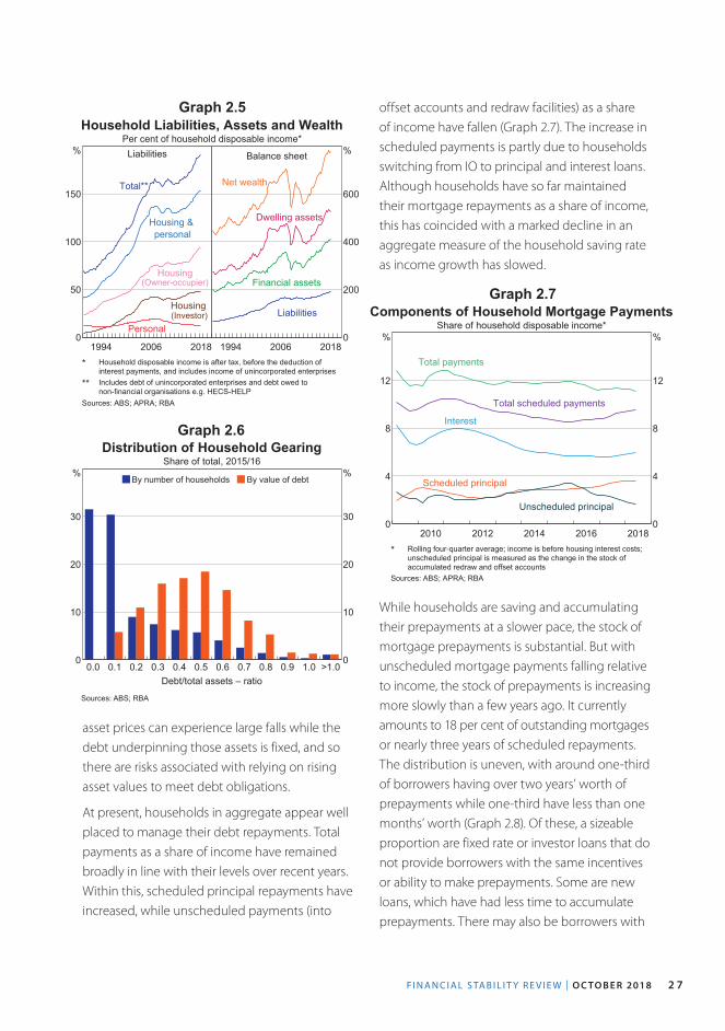
F I N A N C I A L S TA B I L I T Y R E V I E W | O C TO B E R 2018 2 7
asset prices can experience large falls while the debt underpinning those assets is fixed, and so there are risks associated with relying on rising asset values to meet debt obligations.
At present, households in aggregate appear well placed to manage their debt repayments. Total payments as a share of income have remained broadly in line with their levels over recent years. Within this, scheduled principal repayments have increased, while unscheduled payments (into
Graph 2.5Household Liabilities, Assets and Wealth
Per cent of household disposable income*Liabilities
20061994 20180
50
100
150
%
Housing(Investor)
Total**
Personal
Housing(Owner-occupier)
Housing &personal
Balance sheet
20061994 20180
200
400
600
%
Financial assets
Net wealth
Liabilities
Dwelling assets
* Household disposable income is after tax, before the deduction ofinterest payments, and includes income of unincorporated enterprises** Includes debt of unincorporated enterprises and debt owed tonon-financial organisations e.g. HECS-HELP
Sources: ABS; APRA; RBA
Graph 2.7
2016201420122010 20180
4
8
12
%
0
4
8
12
%
Components of Household Mortgage PaymentsShare of household disposable income*
Scheduled principal
Interest
Total payments
Total scheduled payments
Unscheduled principal
* Rolling four-quarter average; income is before housing interest costs;unscheduled principal is measured as the change in the stock ofaccumulated redraw and offset accounts
Sources: ABS; APRA; RBA
offset accounts and redraw facilities) as a share of income have fallen (Graph 2.7). The increase in scheduled payments is partly due to households switching from IO to principal and interest loans. Although households have so far maintained their mortgage repayments as a share of income, this has coincided with a marked decline in an aggregate measure of the household saving rate as income growth has slowed.
Graph 2.6
By number of households By value of debt
0.0 0.1 0.2 0.3 0.4 0.5 0.6 0.7 0.8 0.9 1.0 >1.00
10
20
30
%
0
10
20
30
%
Debt/total assets – ratio
Distribution of Household GearingShare of total, 2015/16
Sources: ABS; RBA
While households are saving and accumulating their prepayments at a slower pace, the stock of mortgage prepayments is substantial. But with unscheduled mortgage payments falling relative to income, the stock of prepayments is increasing more slowly than a few years ago. It currently amounts to 18 per cent of outstanding mortgages or nearly three years of scheduled repayments. The distribution is uneven, with around one-third of borrowers having over two years’ worth of prepayments while one-third have less than one months’ worth (Graph 2.8). Of these, a sizeable proportion are fixed rate or investor loans that do not provide borrowers with the same incentives or ability to make prepayments. Some are new loans, which have had less time to accumulate prepayments. There may also be borrowers with
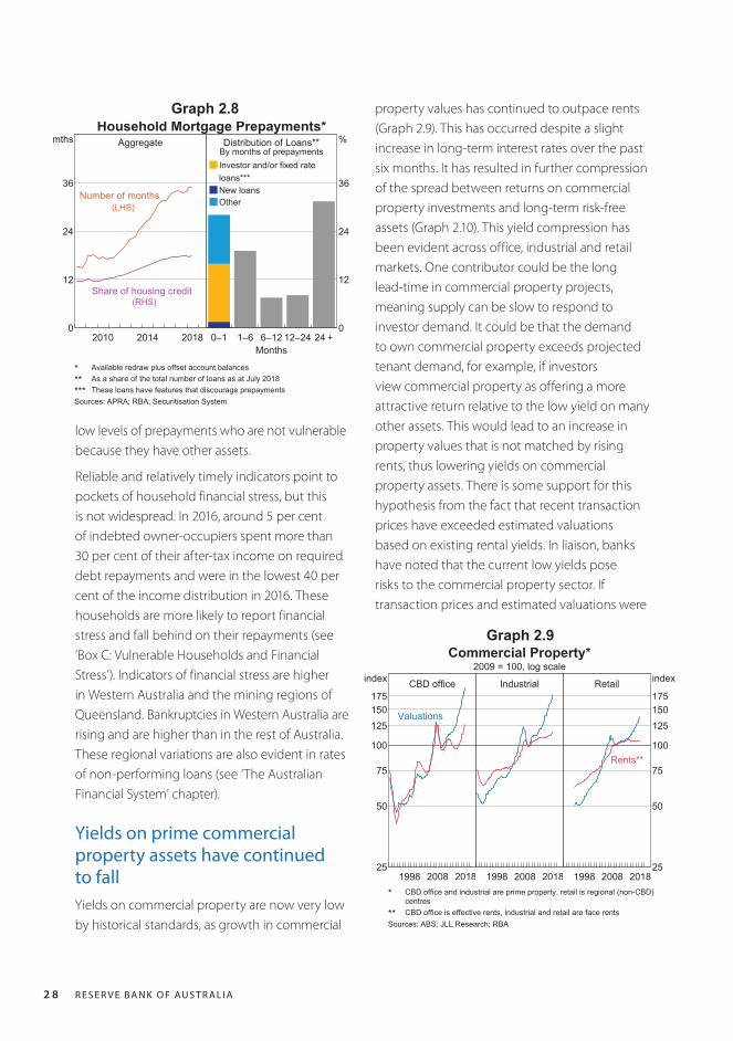
R E S E R V E B A N K O F AU S T R A L I A2 8
low levels of prepayments who are not vulnerable because they have other assets.
Reliable and relatively timely indicators point to pockets of household financial stress, but this is not widespread. In 2016, around 5 per cent of indebted owner-occupiers spent more than 30 per cent of their after-tax income on required debt repayments and were in the lowest 40 per cent of the income distribution in 2016. These households are more likely to report financial stress and fall behind on their repayments (see ‘Box C: Vulnerable Households and Financial Stress’). Indicators of financial stress are higher in Western Australia and the mining regions of Queensland. Bankruptcies in Western Australia are rising and are higher than in the rest of Australia. These regional variations are also evident in rates of non-performing loans (see ‘The Australian Financial System’ chapter).
Yields on prime commercial property assets have continued to fallYields on commercial property are now very low by historical standards, as growth in commercial
property values has continued to outpace rents (Graph 2.9). This has occurred despite a slight increase in long-term interest rates over the past six months. It has resulted in further compression of the spread between returns on commercial property investments and long-term risk-free assets (Graph 2.10). This yield compression has been evident across office, industrial and retail markets. One contributor could be the long lead-time in commercial property projects, meaning supply can be slow to respond to investor demand. It could be that the demand to own commercial property exceeds projected tenant demand, for example, if investors view commercial property as offering a more attractive return relative to the low yield on many other assets. This would lead to an increase in property values that is not matched by rising rents, thus lowering yields on commercial property assets. There is some support for this hypothesis from the fact that recent transaction prices have exceeded estimated valuations based on existing rental yields. In liaison, banks have noted that the current low yields pose risks to the commercial property sector. If transaction prices and estimated valuations were
Graph 2.9Commercial Property*
2009 = 100, log scale
CBD office
20081998 201825
50
75
100
125150175
index
Valuations
Industrial
20081998 2018
Retail
20081998 201825
50
75
100
125150175
index
Rents**
* CBD office and industrial are prime property, retail is regional (non-CBD)centres** CBD office is effective rents, industrial and retail are face rents
Sources: ABS; JLL Research; RBA
Graph 2.8Household Mortgage Prepayments*
Aggregate
20142010 20180
12
24
36
mths
(LHS)Number of months
(RHS)Share of housing credit
Distribution of Loans**By months of prepaymentsInvestor and/or fixed rateloans***New loansOther
0–1 1–6 6–12 12–24 24 +0
12
24
36
%
Months* Available redraw plus offset account balances** As a share of the total number of loans as at July 2018*** These loans have features that discourage prepaymentsSources: APRA; RBA; Securitisation System
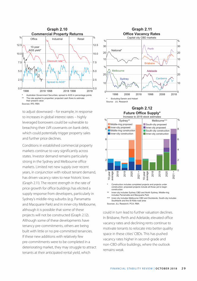
F I N A N C I A L S TA B I L I T Y R E V I E W | O C TO B E R 2018 2 9
Graph 2.10Commercial Property Returns
Office
1998 20180.0
2.5
5.0
7.5
10.0
12.5
%
10-yearAGS yield*
Industrial
1998 2018
Discount rate**
Spread to AGS*
Retail
1998 20180.0
2.5
5.0
7.5
10.0
12.5
%
* Australian Government Securities; spread to AGS in percentage points** The rate applied to properties’ projected cash flows to estimatetheir present value
Sources: IPD; RBA
to adjust downward – for example, in response to increases in global interest rates – highly leveraged borrowers could be vulnerable to breaching their LVR covenants on bank debt, which could potentially trigger property sales and further price declines.
Conditions in established commercial property markets continue to vary significantly across states. Investor demand remains particularly strong in the Sydney and Melbourne office markets. Limited net new supply over recent years, in conjunction with robust tenant demand, has driven vacancy rates to near historic lows (Graph 2.11). The recent strength in the rate of price growth for office buildings has elicited a supply response from developers, particularly in Sydney’s middle-ring suburbs (e.g. Parramatta and Macquarie Park) and in inner-city Melbourne, although it is possible that some of these projects will not be constructed (Graph 2.12). Although some of these developments have tenancy pre-commitments, others are being built with little or no pre-committed tenancies. If these new additions with relatively few pre-commitments were to be completed in a deteriorating market, they may struggle to attract tenants at their anticipated rental yield, which
Graph 2.11Office Vacancy Rates
Capital city CBD markets
10
20
30
%
National*
10
20
30
%
Brisbane
Perth
20081998 20180
10
20
%Melbourne
Sydney
20081998 20180
10
20
%Adelaide
Canberra
* Excluding Darwin and HobartSource: JLL Research
Graph 2.12Future Office Supply*Increase to 2018 stock estimates
Sydney**Middle-ring proposedInner-city proposedMiddle-ring constructionInner-city construction
10-y
ear
aver
age
2018
2019
2020
2021
+0
2
4
6
8
% Melbourne***South-city proposedInner-city proposedSouth-city constructionInner-city construction
10-y
ear
aver
age
2018
2019
2020
2021
+ 0
2
4
6
8
%
* Construction includes completed projects and projects underconstruction; proposed projects include all those yet to beginconstruction** Inner-city includes Sydney CBD and North Sydney; Middle-ringincludes Parramatta and Macquarie Park*** Inner-city includes Melbourne CBD and Docklands; South-city includesSouthbank and the St Kilda road area
Sources: JLL Research; PCA; RBA
could in turn lead to further valuation declines. In Brisbane, Perth and Adelaide, elevated office vacancy rates and declining rents continue to motivate tenants to relocate into better quality space in these cities’ CBDs. This has pushed vacancy rates higher in second-grade and non-CBD office buildings, where the outlook remains weak.
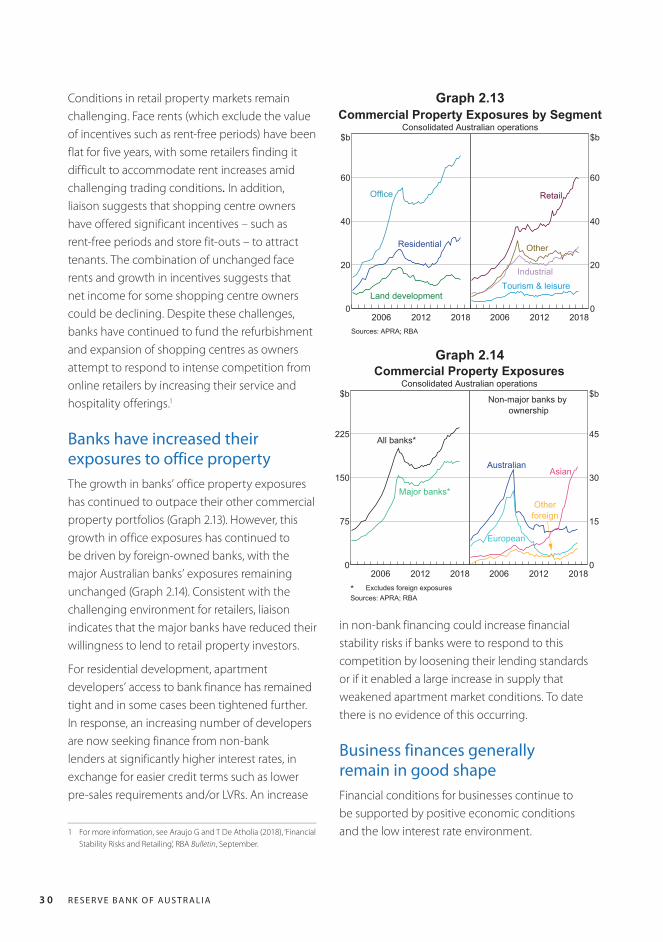
R E S E R V E B A N K O F AU S T R A L I A3 0
Conditions in retail property markets remain challenging. Face rents (which exclude the value of incentives such as rent-free periods) have been flat for five years, with some retailers finding it difficult to accommodate rent increases amid challenging trading conditions. In addition, liaison suggests that shopping centre owners have offered significant incentives – such as rent-free periods and store fit-outs – to attract tenants. The combination of unchanged face rents and growth in incentives suggests that net income for some shopping centre owners could be declining. Despite these challenges, banks have continued to fund the refurbishment and expansion of shopping centres as owners attempt to respond to intense competition from online retailers by increasing their service and hospitality offerings.1
Banks have increased their exposures to office propertyThe growth in banks’ office property exposures has continued to outpace their other commercial property portfolios (Graph 2.13). However, this growth in office exposures has continued to be driven by foreign-owned banks, with the major Australian banks’ exposures remaining unchanged (Graph 2.14). Consistent with the challenging environment for retailers, liaison indicates that the major banks have reduced their willingness to lend to retail property investors.
For residential development, apartment developers’ access to bank finance has remained tight and in some cases been tightened further. In response, an increasing number of developers are now seeking finance from non-bank lenders at significantly higher interest rates, in exchange for easier credit terms such as lower pre-sales requirements and/or LVRs. An increase
1 For more information, see Araujo G and T De Atholia (2018), ‘Financial Stability Risks and Retailing’, RBA Bulletin, September.
in non-bank financing could increase financial stability risks if banks were to respond to this competition by loosening their lending standards or if it enabled a large increase in supply that weakened apartment market conditions. To date there is no evidence of this occurring.
Business finances generally remain in good shapeFinancial conditions for businesses continue to be supported by positive economic conditions and the low interest rate environment.
Graph 2.13Commercial Property Exposures by Segment
Consolidated Australian operations
20122006 20180
20
40
60
$b
Office
Residential
Land development
20122006 20180
20
40
60
$b
Industrial
Other
Tourism & leisure
Retail
Sources: APRA; RBA
Graph 2.14Commercial Property Exposures
Consolidated Australian operations
20122006 20180
75
150
225
$b
All banks*
Major banks*
Non-major banks byownership
20122006 20180
15
30
45
$b
European
Australian
Otherforeign
Asian
* Excludes foreign exposuresSources: APRA; RBA
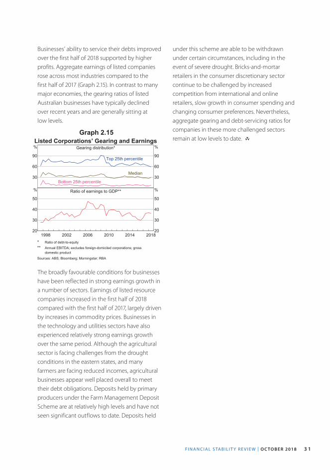
F I N A N C I A L S TA B I L I T Y R E V I E W | O C TO B E R 2018 3 1
Businesses’ ability to service their debts improved over the first half of 2018 supported by higher profits. Aggregate earnings of listed companies rose across most industries compared to the first half of 2017 (Graph 2.15). In contrast to many major economies, the gearing ratios of listed Australian businesses have typically declined over recent years and are generally sitting at low levels.
Graph 2.15Listed Corporations’ Gearing and Earnings
Gearing distribution*
30
60
90
%
30
60
90
%
Top 25th percentile
Median
Bottom 25th percentile
Ratio of earnings to GDP**
20142010200620021998 201820
30
40
50
%
20
30
40
50
%
* Ratio of debt-to-equity** Annual EBITDA; excludes foreign-domiciled corporations; grossdomestic product
Sources: ABS; Bloomberg; Morningstar; RBA
The broadly favourable conditions for businesses have been reflected in strong earnings growth in a number of sectors. Earnings of listed resource companies increased in the first half of 2018 compared with the first half of 2017, largely driven by increases in commodity prices. Businesses in the technology and utilities sectors have also experienced relatively strong earnings growth over the same period. Although the agricultural sector is facing challenges from the drought conditions in the eastern states, and many farmers are facing reduced incomes, agricultural businesses appear well placed overall to meet their debt obligations. Deposits held by primary producers under the Farm Management Deposit Scheme are at relatively high levels and have not seen significant outflows to date. Deposits held
under this scheme are able to be withdrawn under certain circumstances, including in the event of severe drought. Bricks-and-mortar retailers in the consumer discretionary sector continue to be challenged by increased competition from international and online retailers, slow growth in consumer spending and changing consumer preferences. Nevertheless, aggregate gearing and debt-servicing ratios for companies in these more challenged sectors remain at low levels to date. R
R E S E R V E B A N K O F AU S T R A L I A32
Box B
The Impact of Lending Standards on Loan Sizes
To determine the maximum amount they are willing to lend to a prospective borrower, lenders consider the borrower’s cash flows. Historically, a commonly used metric for this purpose was the debt servicing ratio (DSR), under which lenders would generally set maximum loan sizes such that the required repayments did not exceed 30 per cent of pre-tax household income. While simple to calculate and explain, such an approach did not factor in many of the specific circumstances of borrowers.
Since around the mid 2000s, lenders have refined their assessments of borrowers’ cash flow that is available to make their debt repayments. This better accounts for variations in household income and family circumstances (recognising, for instance, that some borrowers can comfortably accommodate DSRs greater than 30 per cent). The methodology and definitions used in undertaking these calculations had varied substantially across lenders. However, in 2015 the Australian Prudential Regulation Authority (APRA) standardised many of the elements of these mortgage loan assessments, bringing tighter standards and greater consistency to the industry. This has tended to reduce the maximum amount that a lender will extend to a new borrower. However, most households choose to borrow much less than the maximum amount offered by lenders. Hence, for the majority of borrowers, this tightening in lending standards will not have had a material effect on their actual access to finance.
This box outlines how lenders’ cash-flow-based calculations interact with the DSR and
other simple serviceability metrics. It also uses household survey data to calculate hypothetical maximum loan sizes of past borrowers and compares these estimates to the amount that they actually borrowed. This enables an assessment of how binding the progressive tightening of the procedures used by lenders has been in practice.
Serviceability tests are now more tailored than in the pastLenders calculate a ‘net income surplus’ (NIS) to help determine the maximum mortgage that could be offered to a potential borrower. Under this approach, a borrower’s estimated living expenses and other existing financial commitments (excluding rental payments) are subtracted from their disposable (i.e. after-tax) income. This determines their ‘net income’, which is the amount available to make debt repayments. The largest possible loan that could be made would leave the borrower with no spare cash after taking account of living expenses and the required annual loan repayments. This maximum loan amount would leave the borrower with a NIS equal to zero. In practice though, lenders incorporate a number of buffers and detail about the borrowers’ circumstances into this calculation, so that a NIS of zero would not mean the borrower had no spare cash flow after repayments (as outlined below).
Unlike the simple DSR, the NIS is tailored for the specific characteristics of each borrower. For example, it allows for the fact that high-income households are usually better able
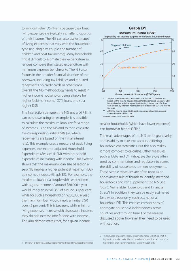
F I N A N C I A L S TA B I L I T Y R E V I E W | O C TO B E R 2018 33
to service higher DSR loans because their basic living expenses are typically a smaller proportion of their income. The NIS can also use estimates of living expenses that vary with the household type (e.g. single vs couple, the number of children and post-tax income). Many households find it difficult to estimate their expenditure so lenders compare their stated expenditure with minimum expense benchmarks. The NIS also factors in the broader financial situation of the borrower, including tax liabilities and required repayments on credit cards or other loans. Overall, the NIS methodology tends to result in higher income households being eligible for higher ‘debt-to-income’ (DTI) loans and so a higher DSR.
The interaction between the NIS and a DSR limit can be shown using an example. It is possible to calculate the maximum loan size for a range of incomes using the NIS and to then calculate the corresponding initial DSRs (i.e. where repayments are based on the initial interest rate). This example uses a measure of basic living expenses, the income-adjusted Household Expenditure Measure (HEM), with household expenditure increasing with income. This exercise shows that the maximum loan size based on a zero NIS implies a higher potential maximum DSR as incomes increase (Graph B1).1 For example, the maximum loan for a couple with two children with a gross income of around $80,000 a year would imply an initial DSR of around 30 per cent while for such a household on $200,000 a year, the maximum loan would imply an initial DSR over 45 per cent. This is because, while minimum living expenses increase with disposable income, they do not increase one for one with income. This also demonstrates that, for a given income,
1 The DSR is defined as actual repayments divided by disposable income.
smaller households (which have lower expenses) can borrow at higher DSRs.2
The main advantages of the NIS are its granularity and its ability to take into account differing household characteristics. But this also makes it more complex to calculate. Other measures, such as DSRs and DTI ratios, are therefore often used by commentators and regulators to assess the ability of households to meet repayments. These simple measures are often used as an approximate rule of thumb to identify stretched households and can supplement the NIS (see ‘Box C: Vulnerable Households and Financial Stress’). In addition, they can be easily estimated for a whole economy, such as a national household DTI. This enables comparisons of aggregate household indebtedness across countries and through time. For the reasons discussed above, however, they need to be used with caution.
2 The NIS also implies the same observations for DTI ratios. That is, higher income households and smaller households can borrow at higher DTIs than lower income or larger households.
40 80 120 160 2000
15
30
45
%
0
15
30
45
%
Gross household income – ($’000/year)
Maximum Initial DSR*Implied by net income surplus for different household types
Single no children
Couple with two children**
* 30-year loan assessed at an interest rate floor of 7.3 per cent andbased on the income-adjusted Household Expenditure Measure; DSRis calculated as initial repayments at starting interest rate of 4.1 percent divided by after-tax income; tax liability based on 2017/18 incometax rates** After-tax income calculated based on each adult earning an equalshare of household income
Sources: Melbourne Institute; RBA
Graph B1
R E S E R V E B A N K O F AU S T R A L I A34
• Applying a ‘haircut’ or discount to income from certain less reliable sources. For example, income earned from overtime or bonuses is typically discounted by 20 per cent. If this income falls, borrowers are then less likely to be caught short. Rental income attracts a similar discount to account for possible tenant vacancies and variability of property management costs and maintenance.
• Minimum expense benchmarks are used as a backstop, such as in situations where borrower-reported expenses are implausibly low.4 Since early 2016, most banks have introduced an upward adjustment to these benchmarks for higher-income borrowers.
• In the case of interest-only loans, the NIS is calculated based on the principal and interest payments that will apply when the interest-only period ends. This buffer alone results in the maximum loan being around 6 per cent lower for a five-year interest-only period within a 30-year loan.
• The NIS test also factors in potential repayment obligations from the full credit limits of existing credit cards (rather than just outstanding balances). More generally, the introduction of the comprehensive credit reporting regime over 2018 and 2019 will give lenders greater visibility of borrowers’ other credit facilities, including credit cards.
4 APRA has outlined instances where lending practices have fallen short of these standards, including an over-reliance on expense benchmarks (which historically have reflected a very basic standard of living) in loan applications. APRA is working with lenders to make improvements, in particular by making more detailed inquiries about borrower expenses and reducing the number of applications based on benchmark expenses.
The NIS incorporates many buffers …Over recent years, APRA has required that banks improve the calculation of the NIS in order to ensure households have an adequate buffer in the event of a shock. In practice, this means that even borrowers who take out the largest loan available and so have a ‘zero NIS’ would initially have spare income after basic living expenses and loan repayments. The effect of these changes, introduced since 2015, has been to reduce the maximum loan size available to borrowers. The buffers include:
• Large interest rate buffers to ensure borrowers can afford to make their repayments if interest rates rise.3 These buffers substantially reduce maximum loan sizes (relative to having no interest rate buffer) and provide a significant amount of spare cash flow. Currently, most loans are assessed at an interest rate of around 7.3 per cent. For a new loan of $500,000 at the current average interest rate of 4.1 per cent repayments would be $950 per month lower than they would be at the buffer interest rate used to calculate the maximum loan size. This amount represents initial cash flow the household could use to make excess repayments or for discretionary consumption, but would be reduced by any future interest rate increases. The maximum loan size available to households is around 30 per cent lower than if there were no buffer.
3 Interest rate buffers were used by lenders before 2015, however there was a wide range used. The APRA measures standardised industry practices by setting the minimum interest rate buffer at 2 percentage points with a further requirement to use an interest rate floor of at least 7 per cent should interest rates be below 5 per cent (as they currently are). Lenders have opted to use buffers a little above the minimum required. Interest rate buffers are also required to be applied to any other existing debts, which had the largest impact on maximum loan sizes for investors with multiple properties.
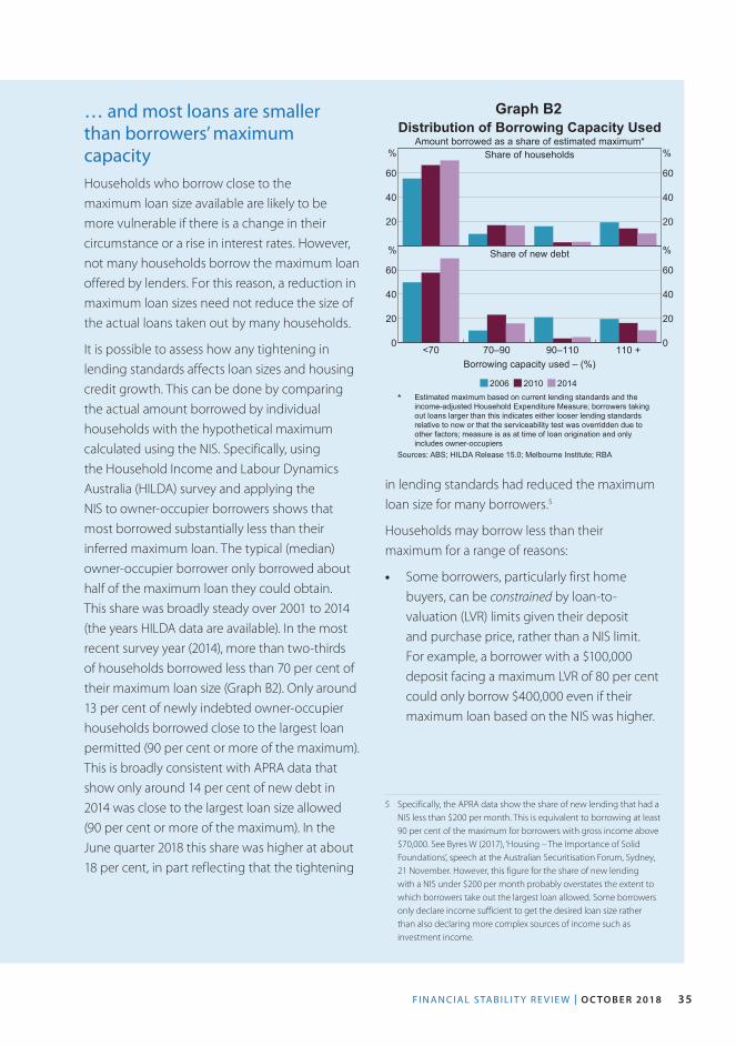
F I N A N C I A L S TA B I L I T Y R E V I E W | O C TO B E R 2018 35
in lending standards had reduced the maximum loan size for many borrowers.5
Households may borrow less than their maximum for a range of reasons:
• Some borrowers, particularly first home buyers, can be constrained by loan-to-valuation (LVR) limits given their deposit and purchase price, rather than a NIS limit. For example, a borrower with a $100,000 deposit facing a maximum LVR of 80 per cent could only borrow $400,000 even if their maximum loan based on the NIS was higher.
5 Specifically, the APRA data show the share of new lending that had a NIS less than $200 per month. This is equivalent to borrowing at least 90 per cent of the maximum for borrowers with gross income above $70,000. See Byres W (2017), ‘Housing – The Importance of Solid Foundations’, speech at the Australian Securitisation Forum, Sydney, 21 November. However, this figure for the share of new lending with a NIS under $200 per month probably overstates the extent to which borrowers take out the largest loan allowed. Some borrowers only declare income sufficient to get the desired loan size rather than also declaring more complex sources of income such as investment income.
… and most loans are smaller than borrowers’ maximum capacity Households who borrow close to the maximum loan size available are likely to be more vulnerable if there is a change in their circumstance or a rise in interest rates. However, not many households borrow the maximum loan offered by lenders. For this reason, a reduction in maximum loan sizes need not reduce the size of the actual loans taken out by many households.
It is possible to assess how any tightening in lending standards affects loan sizes and housing credit growth. This can be done by comparing the actual amount borrowed by individual households with the hypothetical maximum calculated using the NIS. Specifically, using the Household Income and Labour Dynamics Australia (HILDA) survey and applying the NIS to owner-occupier borrowers shows that most borrowed substantially less than their inferred maximum loan. The typical (median) owner-occupier borrower only borrowed about half of the maximum loan they could obtain. This share was broadly steady over 2001 to 2014 (the years HILDA data are available). In the most recent survey year (2014), more than two-thirds of households borrowed less than 70 per cent of their maximum loan size (Graph B2). Only around 13 per cent of newly indebted owner-occupier households borrowed close to the largest loan permitted (90 per cent or more of the maximum). This is broadly consistent with APRA data that show only around 14 per cent of new debt in 2014 was close to the largest loan size allowed (90 per cent or more of the maximum). In the June quarter 2018 this share was higher at about 18 per cent, in part reflecting that the tightening
Distribution of Borrowing Capacity UsedAmount borrowed as a share of estimated maximum*
Share of households
20
40
60
%
20
40
60
%
Share of new debt
<70 70–90 90–110 110 +0
20
40
60
%
0
20
40
60
%
Borrowing capacity used – (%)
2006 2010 2014* Estimated maximum based on current lending standards and theincome-adjusted Household Expenditure Measure; borrowers takingout loans larger than this indicates either looser lending standardsrelative to now or that the serviceability test was overridden due toother factors; measure is as at time of loan origination and onlyincludes owner-occupiers
Sources: ABS; HILDA Release 15.0; Melbourne Institute; RBA
Graph B2
R E S E R V E B A N K O F AU S T R A L I A36
HILDA data indicate that households who borrowed close to the largest amount they could were almost entirely at the lower end of the income distribution of mortgagor households. There were very few borrowers in the top two income quintiles who borrowed close to their maximum. This could be because lower and middle income households had to borrow the most they could in order to enter the housing market, whereas higher income households were less compelled to do so.
However, this analysis overlooks the impact on demand of tighter lending standards, which is hard to quantify. For example, in response to being offered a smaller loan, prospective borrowers may purchase a cheaper dwelling, or save for longer and delay their purchase, or even exit the market entirely. Further, tighter lending standards and greater public scrutiny of lending practices could also weigh on sentiment and reduce demand.
Hence, the calibrated adjustments to lending standards introduced to improve the resilience of households appear to have had the most impact on households choosing to borrow close to their limit. Reducing the risk these borrowers and their lenders were taking on has been desirable from a financial stability perspective. In contrast, the majority of borrowers have not been constrained by the tightening in lending standards. This is consistent with the fact that, to date, owner-occupier credit growth has only slowed modestly. R
• Some households may not need the maximum loan to purchase the dwelling they want.
• Other households, especially ‘trade-up’ buyers, may take a smaller loan to avoid being overleveraged. For example, they may want to be able to make prepayments on their mortgage or have a larger buffer than the minimum required to cover adverse events. Alternatively, they may anticipate future drops in income (for example, time out from the workforce to have children).
So tighter lending standards do not constrain most borrowers, but do affect someMost households in the HILDA sample borrowed well under the maximum implied by the NIS. This behaviour has been reasonably stable over the 14 years of the HILDA surveys, and if households have continued to borrow conservatively, then most households would not have been constrained by the tightening in lending standards over recent years. If households continued to borrow well under their maximum, this implies that even fairly large reductions in maximum loan sizes would have only a modest effect on the supply of new lending. This is consistent with loan approvals data showing that the average owner-occupier loan size has increased from around $350,000 in the first half of 2015 to $410,000 in June 2018, even though lending standards have tightened. Indeed, current lending standards suggest that the maximum loan size that would be offered to the median borrower is between $530,000 and $630,000, well above the typical actual loan taken.
Lower income households would have been more affected than others because more of them borrow close to their maximum. The
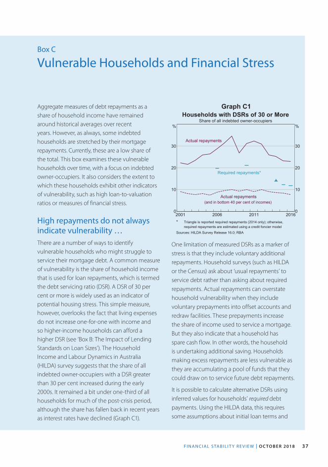
F I N A N C I A L S TA B I L I T Y R E V I E W | O C TO B E R 2018 37
Box C
Vulnerable Households and Financial Stress
Aggregate measures of debt repayments as a share of household income have remained around historical averages over recent years. However, as always, some indebted households are stretched by their mortgage repayments. Currently, these are a low share of the total. This box examines these vulnerable households over time, with a focus on indebted owner-occupiers. It also considers the extent to which these households exhibit other indicators of vulnerability, such as high loan-to-valuation ratios or measures of financial stress.
High repayments do not always indicate vulnerability …There are a number of ways to identify vulnerable households who might struggle to service their mortgage debt. A common measure of vulnerability is the share of household income that is used for loan repayments, which is termed the debt servicing ratio (DSR). A DSR of 30 per cent or more is widely used as an indicator of potential housing stress. This simple measure, however, overlooks the fact that living expenses do not increase one-for-one with income and so higher-income households can afford a higher DSR (see ‘Box B: The Impact of Lending Standards on Loan Sizes’). The Household Income and Labour Dynamics in Australia (HILDA) survey suggests that the share of all indebted owner-occupiers with a DSR greater than 30 per cent increased during the early 2000s. It remained a bit under one-third of all households for much of the post-crisis period, although the share has fallen back in recent years as interest rates have declined (Graph C1).
One limitation of measured DSRs as a marker of stress is that they include voluntary additional repayments. Household surveys (such as HILDA or the Census) ask about ‘usual repayments’ to service debt rather than asking about required repayments. Actual repayments can overstate household vulnerability when they include voluntary prepayments into offset accounts and redraw facilities. These prepayments increase the share of income used to service a mortgage. But they also indicate that a household has spare cash flow. In other words, the household is undertaking additional saving. Households making excess repayments are less vulnerable as they are accumulating a pool of funds that they could draw on to service future debt repayments.
It is possible to calculate alternative DSRs using inferred values for households’ required debt payments. Using the HILDA data, this requires some assumptions about initial loan terms and
2001 2006 2011 20160
10
20
30
%
0
10
20
30
%
Households with DSRs of 30 or MoreShare of all indebted owner-occupiers
Actual repayments
Required repayments*
Actual repayments(and in bottom 40 per cent of incomes)
* Triangle is reported required repayments (2014 only); otherwise,required repayments are estimated using a credit foncier model
Sources: HILDA Survey Release 16.0; RBA
Graph C1
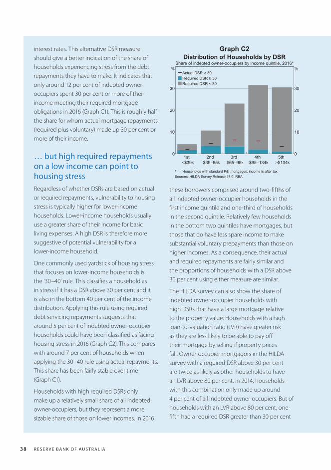
R E S E R V E B A N K O F AU S T R A L I A38
interest rates. This alternative DSR measure should give a better indication of the share of households experiencing stress from the debt repayments they have to make. It indicates that only around 12 per cent of indebted owner-occupiers spent 30 per cent or more of their income meeting their required mortgage obligations in 2016 (Graph C1). This is roughly half the share for whom actual mortgage repayments (required plus voluntary) made up 30 per cent or more of their income.
… but high required repayments on a low income can point to housing stressRegardless of whether DSRs are based on actual or required repayments, vulnerability to housing stress is typically higher for lower-income households. Lower-income households usually use a greater share of their income for basic living expenses. A high DSR is therefore more suggestive of potential vulnerability for a lower-income household.
One commonly used yardstick of housing stress that focuses on lower-income households is the ‘30–40’ rule. This classifies a household as in stress if it has a DSR above 30 per cent and it is also in the bottom 40 per cent of the income distribution. Applying this rule using required debt servicing repayments suggests that around 5 per cent of indebted owner-occupier households could have been classified as facing housing stress in 2016 (Graph C2). This compares with around 7 per cent of households when applying the 30–40 rule using actual repayments. This share has been fairly stable over time (Graph C1).
Households with high required DSRs only make up a relatively small share of all indebted owner-occupiers, but they represent a more sizable share of those on lower incomes. In 2016
these borrowers comprised around two-fifths of all indebted owner-occupier households in the first income quintile and one-third of households in the second quintile. Relatively few households in the bottom two quintiles have mortgages, but those that do have less spare income to make substantial voluntary prepayments than those on higher incomes. As a consequence, their actual and required repayments are fairly similar and the proportions of households with a DSR above 30 per cent using either measure are similar.
The HILDA survey can also show the share of indebted owner-occupier households with high DSRs that have a large mortgage relative to the property value. Households with a high loan-to-valuation ratio (LVR) have greater risk as they are less likely to be able to pay off their mortgage by selling if property prices fall. Owner-occupier mortgagors in the HILDA survey with a required DSR above 30 per cent are twice as likely as other households to have an LVR above 80 per cent. In 2014, households with this combination only made up around 4 per cent of all indebted owner-occupiers. But of households with an LVR above 80 per cent, one-fifth had a required DSR greater than 30 per cent
Actual DSR ≥ 30Required DSR ≥ 30Required DSR < 30
1st<$39k
2nd$39–65k
3rd$65–95k
4th$95–134k
5th>$134k
0
10
20
30
%
0
10
20
30
%
Distribution of Households by DSRShare of indebted owner-occupiers by income quintile, 2016*
* Households with standard P&I mortgages; income is after taxSources: HILDA Survey Release 16.0; RBA
Graph C2
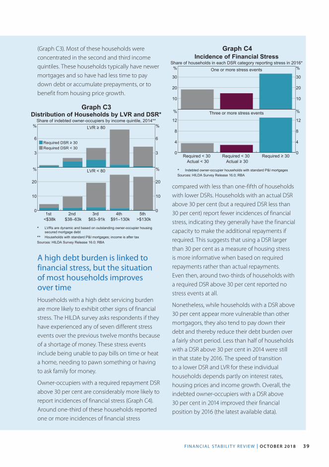
F I N A N C I A L S TA B I L I T Y R E V I E W | O C TO B E R 2018 39
compared with less than one-fifth of households with lower DSRs. Households with an actual DSR above 30 per cent (but a required DSR less than 30 per cent) report fewer incidences of financial stress, indicating they generally have the financial capacity to make the additional repayments if required. This suggests that using a DSR larger than 30 per cent as a measure of housing stress is more informative when based on required repayments rather than actual repayments. Even then, around two-thirds of households with a required DSR above 30 per cent reported no stress events at all.
Nonetheless, while households with a DSR above 30 per cent appear more vulnerable than other mortgagors, they also tend to pay down their debt and thereby reduce their debt burden over a fairly short period. Less than half of households with a DSR above 30 per cent in 2014 were still in that state by 2016. The speed of transition to a lower DSR and LVR for these individual households depends partly on interest rates, housing prices and income growth. Overall, the indebted owner-occupiers with a DSR above 30 per cent in 2014 improved their financial position by 2016 (the latest available data).
A high debt burden is linked to financial stress, but the situation of most households improves over time Households with a high debt servicing burden are more likely to exhibit other signs of financial stress. The HILDA survey asks respondents if they have experienced any of seven different stress events over the previous twelve months because of a shortage of money. These stress events include being unable to pay bills on time or heat a home, needing to pawn something or having to ask family for money.
Owner-occupiers with a required repayment DSR above 30 per cent are considerably more likely to report incidences of financial stress (Graph C4). Around one-third of these households reported one or more incidences of financial stress
Distribution of Households by LVR and DSR*Share of indebted owner-occupiers by income quintile, 2014**
LVR ≥ 80
Required DSR ≥ 30Required DSR < 30
3
6
%
3
6
%
LVR < 80
1st<$38k
2nd$38–63k
3rd$63–91k
4th$91–130k
5th>$130k
0
10
20
%
0
10
20
%
* LVRs are dynamic and based on outstanding owner-occupier housingsecured mortgage debt** Households with standard P&I mortgages; income is after tax
Sources: HILDA Survey Release 16.0; RBA
Graph C3
Incidence of Financial StressShare of households in each DSR category reporting stress in 2016*
One or more stress events
10
20
30
%
10
20
30
%
Three or more stress events
Required < 30Actual < 30
Required < 30Actual ≥ 30
Required ≥ 300
4
8
12
%
0
4
8
12
%
* Indebted owner-occupier households with standard P&I mortgagesSources: HILDA Survey Release 16.0; RBA
Graph C4(Graph C3). Most of these households were concentrated in the second and third income quintiles. These households typically have newer mortgages and so have had less time to pay down debt or accumulate prepayments, or to benefit from housing price growth.

R E S E R V E B A N K O F AU S T R A L I A40
Although median outstanding mortgage debt only declined marginally, household income rose by around one-fifth, and the median required DSR fell by the same degree.1 However, as the debt burden of these households declines, a new cohort of borrowers come along with new mortgages, a small number of whom have a high DSR and high LVR at loan origination and hence can be potentially vulnerable to economic shocks. R
1 Income for these households may grow strongly because a household member earns a promotion, or a second income-earner re-enters the workforce.
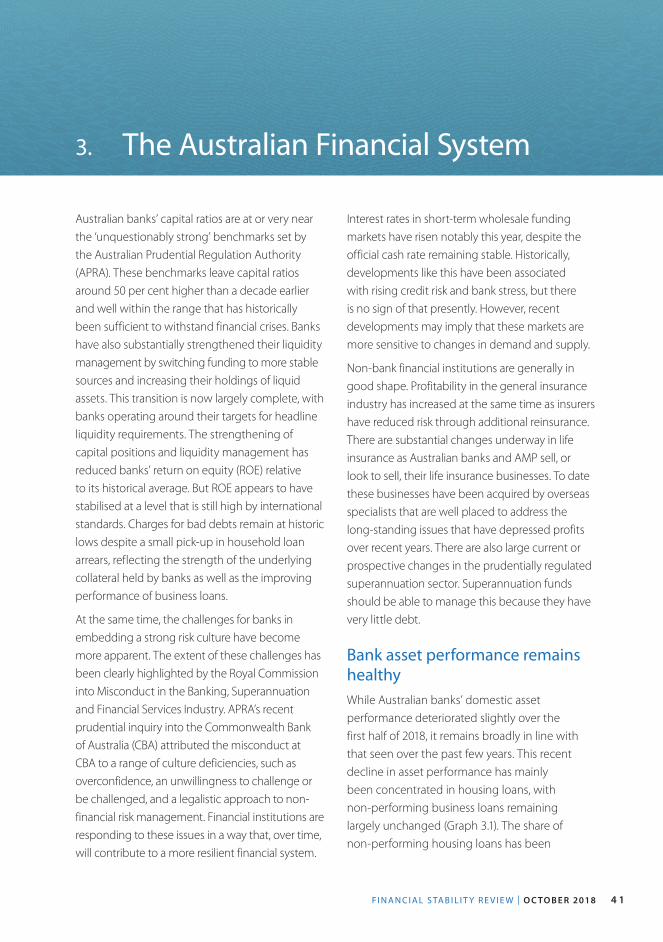
F I N A N C I A L S TA B I L I T Y R E V I E W | O C TO B E R 2018 4 1
3. The Australian Financial System
Australian banks’ capital ratios are at or very near the ‘unquestionably strong’ benchmarks set by the Australian Prudential Regulation Authority (APRA). These benchmarks leave capital ratios around 50 per cent higher than a decade earlier and well within the range that has historically been sufficient to withstand financial crises. Banks have also substantially strengthened their liquidity management by switching funding to more stable sources and increasing their holdings of liquid assets. This transition is now largely complete, with banks operating around their targets for headline liquidity requirements. The strengthening of capital positions and liquidity management has reduced banks’ return on equity (ROE) relative to its historical average. But ROE appears to have stabilised at a level that is still high by international standards. Charges for bad debts remain at historic lows despite a small pick-up in household loan arrears, reflecting the strength of the underlying collateral held by banks as well as the improving performance of business loans.
At the same time, the challenges for banks in embedding a strong risk culture have become more apparent. The extent of these challenges has been clearly highlighted by the Royal Commission into Misconduct in the Banking, Superannuation and Financial Services Industry. APRA’s recent prudential inquiry into the Commonwealth Bank of Australia (CBA) attributed the misconduct at CBA to a range of culture deficiencies, such as overconfidence, an unwillingness to challenge or be challenged, and a legalistic approach to non-financial risk management. Financial institutions are responding to these issues in a way that, over time, will contribute to a more resilient financial system.
Interest rates in short-term wholesale funding markets have risen notably this year, despite the official cash rate remaining stable. Historically, developments like this have been associated with rising credit risk and bank stress, but there is no sign of that presently. However, recent developments may imply that these markets are more sensitive to changes in demand and supply.
Non-bank financial institutions are generally in good shape. Profitability in the general insurance industry has increased at the same time as insurers have reduced risk through additional reinsurance. There are substantial changes underway in life insurance as Australian banks and AMP sell, or look to sell, their life insurance businesses. To date these businesses have been acquired by overseas specialists that are well placed to address the long-standing issues that have depressed profits over recent years. There are also large current or prospective changes in the prudentially regulated superannuation sector. Superannuation funds should be able to manage this because they have very little debt.
Bank asset performance remains healthyWhile Australian banks’ domestic asset performance deteriorated slightly over the first half of 2018, it remains broadly in line with that seen over the past few years. This recent decline in asset performance has mainly been concentrated in housing loans, with non-performing business loans remaining largely unchanged (Graph 3.1). The share of non-performing housing loans has been
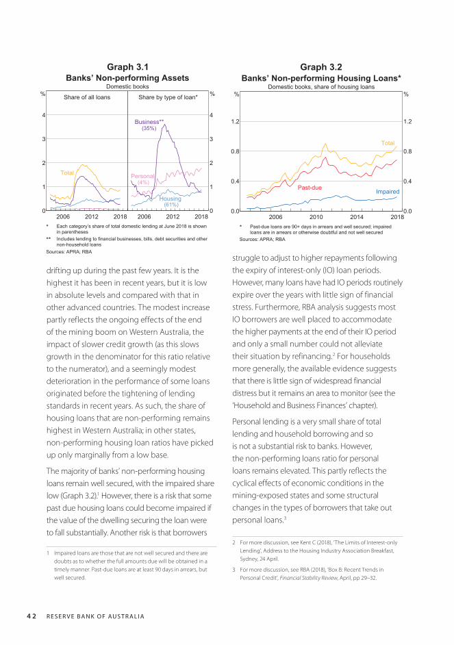
R E S E R V E B A N K O F AU S T R A L I A4 2
drifting up during the past few years. It is the highest it has been in recent years, but it is low in absolute levels and compared with that in other advanced countries. The modest increase partly reflects the ongoing effects of the end of the mining boom on Western Australia, the impact of slower credit growth (as this slows growth in the denominator for this ratio relative to the numerator), and a seemingly modest deterioration in the performance of some loans originated before the tightening of lending standards in recent years. As such, the share of housing loans that are non-performing remains highest in Western Australia; in other states, non-performing housing loan ratios have picked up only marginally from a low base.
The majority of banks’ non-performing housing loans remain well secured, with the impaired share low (Graph 3.2).1 However, there is a risk that some past due housing loans could become impaired if the value of the dwelling securing the loan were to fall substantially. Another risk is that borrowers
1 Impaired loans are those that are not well secured and there are doubts as to whether the full amounts due will be obtained in a timely manner. Past-due loans are at least 90 days in arrears, but well secured.
struggle to adjust to higher repayments following the expiry of interest-only (IO) loan periods. However, many loans have had IO periods routinely expire over the years with little sign of financial stress. Furthermore, RBA analysis suggests most IO borrowers are well placed to accommodate the higher payments at the end of their IO period and only a small number could not alleviate their situation by refinancing.2 For households more generally, the available evidence suggests that there is little sign of widespread financial distress but it remains an area to monitor (see the ‘Household and Business Finances’ chapter).
Personal lending is a very small share of total lending and household borrowing and so is not a substantial risk to banks. However, the non-performing loans ratio for personal loans remains elevated. This partly reflects the cyclical effects of economic conditions in the mining-exposed states and some structural changes in the types of borrowers that take out personal loans.3
2 For more discussion, see Kent C (2018), ‘The Limits of Interest-only Lending’, Address to the Housing Industry Association Breakfast, Sydney, 24 April.
3 For more discussion, see RBA (2018), ‘Box B: Recent Trends in Personal Credit’, Financial Stability Review, April, pp 29–32.
Graph 3.1 Graph 3.2Banks’ Non-performing Assets
Domestic books
Share of all loans
20122006 20180
1
2
3
4
%
Total
Share by type of loan*
20122006 20180
1
2
3
4
%
Personal
Housing
(4%)
Business**(35%)
(61%)
* Each category’s share of total domestic lending at June 2018 is shownin parentheses** Includes lending to financial businesses, bills, debt securities and othernon-household loans
Sources: APRA; RBA
201420102006 20180.0
0.4
0.8
1.2
%
0.0
0.4
0.8
1.2
%
Banks’ Non-performing Housing Loans*Domestic books, share of housing loans
Past-due
Total
Impaired
* Past-due loans are 90+ days in arrears and well secured; impairedloans are in arrears or otherwise doubtful and not well secured
Sources: APRA; RBA
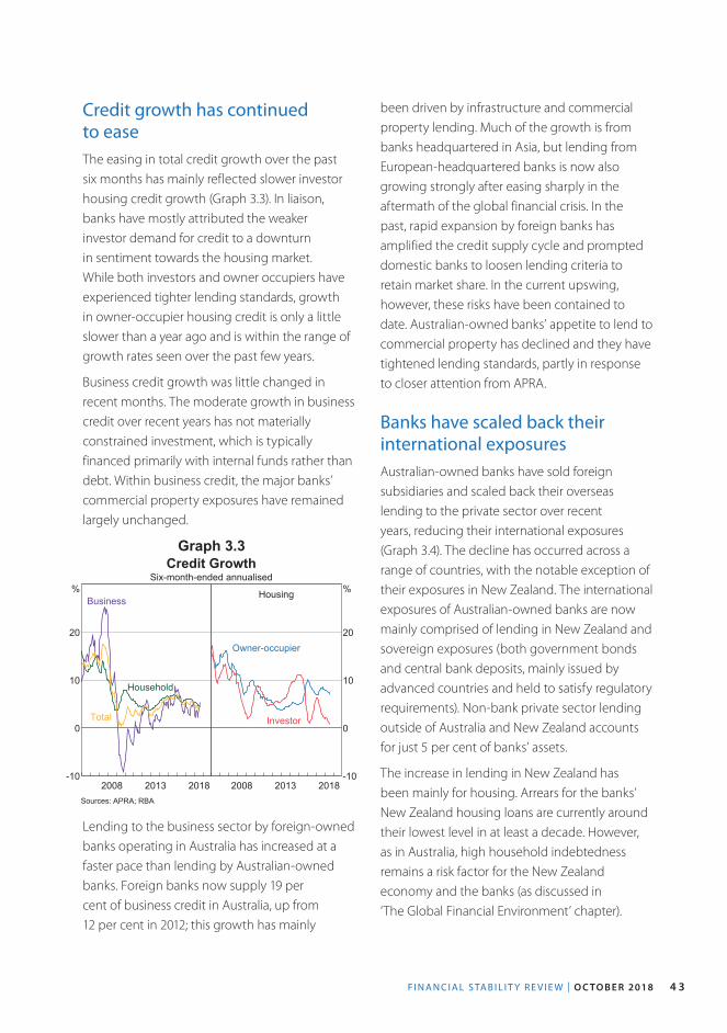
F I N A N C I A L S TA B I L I T Y R E V I E W | O C TO B E R 2018 4 3
Credit growth has continued to easeThe easing in total credit growth over the past six months has mainly reflected slower investor housing credit growth (Graph 3.3). In liaison, banks have mostly attributed the weaker investor demand for credit to a downturn in sentiment towards the housing market. While both investors and owner occupiers have experienced tighter lending standards, growth in owner-occupier housing credit is only a little slower than a year ago and is within the range of growth rates seen over the past few years.
Business credit growth was little changed in recent months. The moderate growth in business credit over recent years has not materially constrained investment, which is typically financed primarily with internal funds rather than debt. Within business credit, the major banks’ commercial property exposures have remained largely unchanged.
been driven by infrastructure and commercial property lending. Much of the growth is from banks headquartered in Asia, but lending from European-headquartered banks is now also growing strongly after easing sharply in the aftermath of the global financial crisis. In the past, rapid expansion by foreign banks has amplified the credit supply cycle and prompted domestic banks to loosen lending criteria to retain market share. In the current upswing, however, these risks have been contained to date. Australian-owned banks’ appetite to lend to commercial property has declined and they have tightened lending standards, partly in response to closer attention from APRA.
Banks have scaled back their international exposuresAustralian-owned banks have sold foreign subsidiaries and scaled back their overseas lending to the private sector over recent years, reducing their international exposures (Graph 3.4). The decline has occurred across a range of countries, with the notable exception of their exposures in New Zealand. The international exposures of Australian-owned banks are now mainly comprised of lending in New Zealand and sovereign exposures (both government bonds and central bank deposits, mainly issued by advanced countries and held to satisfy regulatory requirements). Non-bank private sector lending outside of Australia and New Zealand accounts for just 5 per cent of banks’ assets.
The increase in lending in New Zealand has been mainly for housing. Arrears for the banks’ New Zealand housing loans are currently around their lowest level in at least a decade. However, as in Australia, high household indebtedness remains a risk factor for the New Zealand economy and the banks (as discussed in ‘The Global Financial Environment’ chapter).
Graph 3.3Credit Growth
Six-month-ended annualised
20132008 2018-10
0
10
20
%
Total
Household
BusinessHousing
20132008 2018-10
0
10
20
%
Owner-occupier
Investor
Sources: APRA; RBA
Lending to the business sector by foreign-owned banks operating in Australia has increased at a faster pace than lending by Australian-owned banks. Foreign banks now supply 19 per cent of business credit in Australia, up from 12 per cent in 2012; this growth has mainly
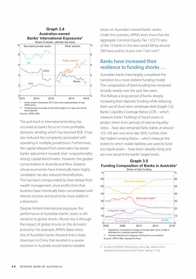
R E S E R V E B A N K O F AU S T R A L I A4 4
The pull-back in international lending has occurred as banks focus on more profitable domestic lending, which has boosted ROE. It has also reduced the complexity associated with operating in multiple jurisdictions. Furthermore, the capital released from asset sales has eased banks’ adjustment towards their ‘unquestionably strong’ capital benchmarks. However, the greater concentration in Australia and New Zealand, whose economies have historically been highly correlated, has also reduced diversification. This has been compounded by their retreat from wealth management, since profits from that business have historically been uncorrelated with interest income and tend to be more stable in a downturn.
Despite limited international exposure, the performance of Australian banks’ assets is still sensitive to global shocks. Mostly this is through the impact of global shocks on the domestic economy. For example, APRA’s latest stress test of Australian banks showed that a sharp downturn in China that resulted in a severe recession in Australia would lead to sizeable
losses on Australian-owned banks’ assets. Under this scenario, APRA’s tests show that the aggregate Common Equity Tier 1 (CET1) ratio of the 13 banks in the test would fall by around 300 basis points, to just over 7 per cent.4
Banks have increased their resilience to funding shocks …Australian banks have largely completed the transition to a more resilient funding model. The composition of bank funding has remained broadly steady over the past few years. This follows a long period of banks sharply increasing their deposits funding while reducing their use of short-term wholesale debt (Graph 3.5). Banks’ Liquidity Coverage Ratios (LCR) – which measure banks’ holdings of liquid assets to protect them from periods of intense liquidity stress – have also remained fairly stable, at around 125–135 per cent since late 2016. Further, their Net Stable Funding Ratios – which measure the extent to which stable liabilities are used to fund less liquid assets – have been steadily rising and are now around the banks’ target levels.
4 See Byres W (2018), ‘Preparing for a rainy day,’ speech at the Australian Business Economists’ Forum, Sydney, 11 July.
Graph 3.4Australian-owned
Banks’ International Exposures*Share of assets, ultimate risk basis
Non-bank private sector
20142010 20180
2
4
6
8
%
Asia
Other
NZ
Other sectors
2014 20180
2
4
6
8
%
Banks
Public sector**
* Series break in December 2017 due to the implementation of newAPRA forms** Predominantly sovereign bonds held outright or on repo and centralbank deposits
Sources: APRA; RBA
Graph 3.5
2014201020062002 20180
10
20
30
40
50
60
%
0
10
20
30
40
50
60
%
Funding Composition of Banks in Australia*Share of total funding
Securitisation Equity
Long-term debt
Domestic deposits
Short-term debt**
* Adjusted for movements in foreign exchange rates; tenor of debt isestimated on a residual maturity basis** Includes deposits and intragroup funding from non-residents
Sources: APRA; RBA; Standard & Poors
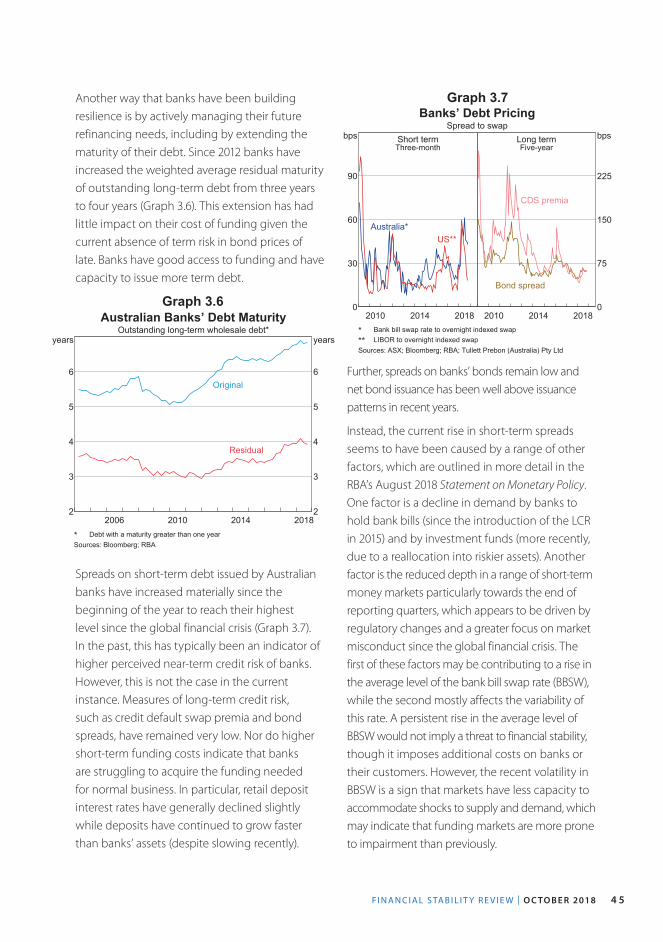
F I N A N C I A L S TA B I L I T Y R E V I E W | O C TO B E R 2018 4 5
Another way that banks have been building resilience is by actively managing their future refinancing needs, including by extending the maturity of their debt. Since 2012 banks have increased the weighted average residual maturity of outstanding long-term debt from three years to four years (Graph 3.6). This extension has had little impact on their cost of funding given the current absence of term risk in bond prices of late. Banks have good access to funding and have capacity to issue more term debt.
Graph 3.6
Graph 3.7
201420102006 20182
3
4
5
6
years
2
3
4
5
6
years
Australian Banks’ Debt MaturityOutstanding long-term wholesale debt*
Residual
Original
* Debt with a maturity greater than one yearSources: Bloomberg; RBA
Banks’ Debt PricingSpread to swap
Short termThree-month
20142010 20180
30
60
90
bps
Australia*US**
Long termFive-year
20142010 20180
75
150
225
bps
CDS premia
Bond spread
* Bank bill swap rate to overnight indexed swap** LIBOR to overnight indexed swapSources: ASX; Bloomberg; RBA; Tullett Prebon (Australia) Pty Ltd
Spreads on short-term debt issued by Australian banks have increased materially since the beginning of the year to reach their highest level since the global financial crisis (Graph 3.7). In the past, this has typically been an indicator of higher perceived near-term credit risk of banks. However, this is not the case in the current instance. Measures of long-term credit risk, such as credit default swap premia and bond spreads, have remained very low. Nor do higher short-term funding costs indicate that banks are struggling to acquire the funding needed for normal business. In particular, retail deposit interest rates have generally declined slightly while deposits have continued to grow faster than banks’ assets (despite slowing recently).
Further, spreads on banks’ bonds remain low and net bond issuance has been well above issuance patterns in recent years.
Instead, the current rise in short-term spreads seems to have been caused by a range of other factors, which are outlined in more detail in the RBA’s August 2018 Statement on Monetary Policy. One factor is a decline in demand by banks to hold bank bills (since the introduction of the LCR in 2015) and by investment funds (more recently, due to a reallocation into riskier assets). Another factor is the reduced depth in a range of short-term money markets particularly towards the end of reporting quarters, which appears to be driven by regulatory changes and a greater focus on market misconduct since the global financial crisis. The first of these factors may be contributing to a rise in the average level of the bank bill swap rate (BBSW), while the second mostly affects the variability of this rate. A persistent rise in the average level of BBSW would not imply a threat to financial stability, though it imposes additional costs on banks or their customers. However, the recent volatility in BBSW is a sign that markets have less capacity to accommodate shocks to supply and demand, which may indicate that funding markets are more prone to impairment than previously.
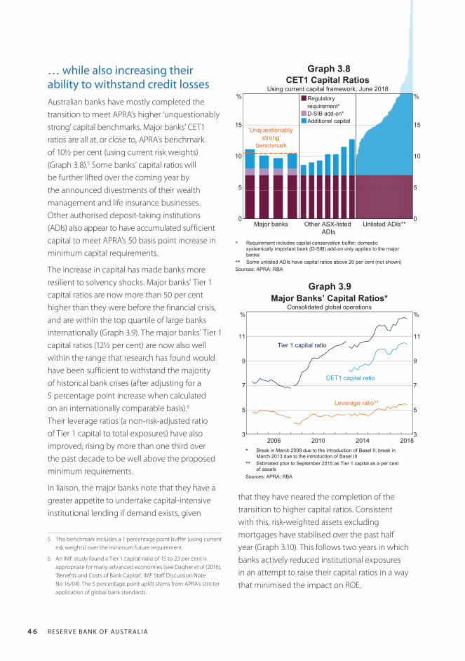
R E S E R V E B A N K O F AU S T R A L I A4 6
… while also increasing their ability to withstand credit lossesAustralian banks have mostly completed the transition to meet APRA’s higher ‘unquestionably strong’ capital benchmarks. Major banks’ CET1 ratios are all at, or close to, APRA’s benchmark of 10½ per cent (using current risk weights) (Graph 3.8).5 Some banks’ capital ratios will be further lifted over the coming year by the announced divestments of their wealth management and life insurance businesses. Other authorised deposit-taking institutions (ADIs) also appear to have accumulated sufficient capital to meet APRA’s 50 basis point increase in minimum capital requirements.
The increase in capital has made banks more resilient to solvency shocks. Major banks’ Tier 1 capital ratios are now more than 50 per cent higher than they were before the financial crisis, and are within the top quartile of large banks internationally (Graph 3.9). The major banks’ Tier 1 capital ratios (12½ per cent) are now also well within the range that research has found would have been sufficient to withstand the majority of historical bank crises (after adjusting for a 5 percentage point increase when calculated on an internationally comparable basis).6 Their leverage ratios (a non-risk-adjusted ratio of Tier 1 capital to total exposures) have also improved, rising by more than one third over the past decade to be well above the proposed minimum requirements.
In liaison, the major banks note that they have a greater appetite to undertake capital-intensive institutional lending if demand exists, given
5 This benchmark includes a 1 percentage point buffer (using current risk weights) over the minimum future requirement.
6 An IMF study found a Tier 1 capital ratio of 15 to 23 per cent is appropriate for many advanced economies (see Dagher et al (2016), ‘Benefits and Costs of Bank Capital’, IMF Staff Discussion Note No 16/04). The 5 percentage point uplift stems from APRA’s stricter application of global bank standards.
that they have neared the completion of the transition to higher capital ratios. Consistent with this, risk-weighted assets excluding mortgages have stabilised over the past half year (Graph 3.10). This follows two years in which banks actively reduced institutional exposures in an attempt to raise their capital ratios in a way that minimised the impact on ROE.
Graph 3.8
Graph 3.9
CET1 Capital RatiosUsing current capital framework, June 2018
0
5
10
15
%
Major banks
‘Unquestionablystrong’
benchmark
Regulatoryrequirement*D-SIB add-on*Additional capital
Other ASX-listedADIs
0
5
10
15
%
Unlisted ADIs**
* Requirement includes capital conservation buffer; domesticsystemically important bank (D-SIB) add-on only applies to the majorbanks** Some unlisted ADIs have capital ratios above 20 per cent (not shown)
Sources: APRA; RBA
201420102006 20183
5
7
9
11
%
3
5
7
9
11
%
Major Banks’ Capital Ratios*Consolidated global operations
Tier 1 capital ratio
CET1 capital ratio
Leverage ratio**
* Break in March 2008 due to the introduction of Basel II; break inMarch 2013 due to the introduction of Basel III** Estimated prior to September 2015 as Tier 1 capital as a per centof assets
Sources: APRA; RBA
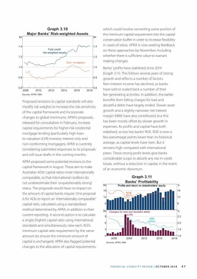
F I N A N C I A L S TA B I L I T Y R E V I E W | O C TO B E R 2018 4 7
which could involve converting some portion of the minimum capital requirement into the capital conservation buffer in order to increase flexibility in cases of stress. APRA is now seeking feedback on these approaches by November, including whether there is sufficient value to warrant making changes.
Banks’ profits have stabilised since 2014 (Graph 3.11). This follows several years of strong growth and reflects a number of factors. Non-interest income has declined, as banks have sold or scaled back a number of their fee-generating activities. In addition, the earlier benefits from falling charges for bad and doubtful debts have largely ended. Slower asset growth and a slightly narrower net interest margin (NIM) have also contributed, but this has been mostly offset by slower growth in expenses. As profits and capital have both stabilised, so too has banks’ ROE. ROE is now a few percentage points lower than its historical average, as capital levels have risen. But it remains high compared with international peers. These strong profit levels give banks considerable scope to absorb any rise in credit losses, without a reduction in capital, in the event of an economic downturn.
Graph 3.10
20162014201220102008 20180.6
0.8
1.0
1.2
1.4
$tr
0.6
0.8
1.0
1.2
1.4
$trMajor Banks’ Risk-weighted Assets
Total creditrisk-weighted assets
Excl. mortgages
Sources: APRA; RBA
Proposed revisions to capital standards will also modify risk weights to increase the risk-sensitivity of the capital framework and incorporate changes to global minimums. APRA’s proposals, released for consultation in February, increase capital requirements for higher-risk residential mortgage lending (particularly high-loan-to-valuation (LVR) investor, interest only and non-conforming mortgages). APRA is currently considering submitted responses to its proposals and will issue drafts in the coming months.
APRA proposed some potential revisions to the capital framework in August. These aim to make Australian ADIs’ capital ratios more internationally comparable, so that international creditors do not underestimate their ‘unquestionably strong’ status. The proposals would have no impact on the amount of capital banks require. One proposal is for ADIs to report an ‘internationally comparable’ capital ratio, calculated using a standardised method determined by APRA, in addition to their current reporting. A second option is to calculate a single (higher) capital ratio using international standards and simultaneously raise each ADI’s minimum capital ratio requirement by the same amount (to ensure the minimum amount of capital is unchanged). APRA also flagged potential changes to the allocation of capital requirements,
Graph 3.11Banks’ Profitability
Profits and return on shareholders’ equityProfits and return on shareholders’ equity
6
12
18
$b
6
12
18
%
(RHS)ROE
2015201220092006 20180
3
6
9
$b
1.6
1.8
2.0
2.2
%
NIM
Charges for bad and doubtful debts(LHS)
(RHS)
Sources: APRA; RBA
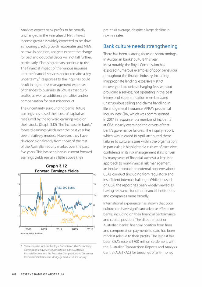
R E S E R V E B A N K O F AU S T R A L I A4 8
Analysts expect bank profits to be broadly unchanged in the year ahead. Net interest income growth is widely expected to be slow as housing credit growth moderates and NIMs narrow. In addition, analysts expect the charge for bad and doubtful debts will not fall further, particularly if housing arrears continue to rise. The financial impact of the various inquiries into the financial services sector remains a key uncertainty.7 Responses to the inquiries could result in higher risk management expenses or changes to business structures that curb profits, as well as additional penalties and/or compensation for past misconduct.
The uncertainty surrounding banks’ future earnings has raised their cost of capital, as measured by the forward earnings yield on their stocks (Graph 3.12). The increase in banks’ forward earnings yields over the past year has been relatively modest. However, they have diverged significantly from those of the rest of the Australian equity market over the past five years. This has seen banks’ current forward earnings yields remain a little above their
7 These inquiries include the Royal Commission, the Productivity Commission’s Inquiry into Competition in the Australian Financial System, and the Australian Competition and Consumer Commission’s Residential Mortgage Products Price Inquiry.
pre-crisis average, despite a large decline in risk-free rates.
Bank culture needs strengtheningThere has been a strong focus on shortcomings in Australian banks’ culture this year. Most notably, the Royal Commission has exposed numerous examples of poor behaviour throughout the finance industry, including: inappropriate lending; excessively strict recovery of bad debts; charging fees without providing a service; not operating in the best interests of superannuation members; and unscrupulous selling and claims handling in life and general insurance. APRA’s prudential inquiry into CBA, which was commissioned in 2017 in response to a number of incidents at CBA, closely examined the drivers of that bank’s governance failures. The inquiry report, which was released in April, attributed these failures to cultural issues within the organisation. In particular, it highlighted a culture of excessive confidence in its risk management skills (driven by many years of financial success), a legalistic approach to non-financial risk management, an insular approach to external concerns about CBA’s conduct (including from regulators) and insufficient internal challenge. While focused on CBA, the report has been widely viewed as having relevance for other financial institutions and companies more broadly.
International experience has shown that poor culture can have significant adverse effects on banks, including on their financial performance and capital position. The direct impact on Australian banks’ financial position from fines and compensation payments to date has been modest relative to their profits. The largest has been CBA’s recent $700 million settlement with the Australian Transactions Reports and Analysis Centre (AUSTRAC) for breaches of anti-money
Graph 3.12
2015201220092006 20184
6
8
10
12
%
4
6
8
10
12
%Forward Earnings Yields
ASX 200
ASX 200 Banks
(excl. banks)
Sources: RBA; Refinitiv
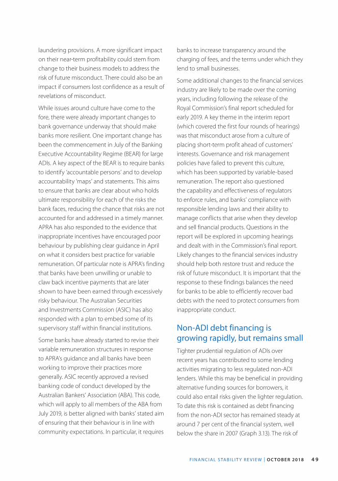
F I N A N C I A L S TA B I L I T Y R E V I E W | O C TO B E R 2018 4 9
laundering provisions. A more significant impact on their near-term profitability could stem from change to their business models to address the risk of future misconduct. There could also be an impact if consumers lost confidence as a result of revelations of misconduct.
While issues around culture have come to the fore, there were already important changes to bank governance underway that should make banks more resilient. One important change has been the commencement in July of the Banking Executive Accountability Regime (BEAR) for large ADIs. A key aspect of the BEAR is to require banks to identify ‘accountable persons’ and to develop accountability ‘maps’ and statements. This aims to ensure that banks are clear about who holds ultimate responsibility for each of the risks the bank faces, reducing the chance that risks are not accounted for and addressed in a timely manner. APRA has also responded to the evidence that inappropriate incentives have encouraged poor behaviour by publishing clear guidance in April on what it considers best practice for variable remuneration. Of particular note is APRA’s finding that banks have been unwilling or unable to claw back incentive payments that are later shown to have been earned through excessively risky behaviour. The Australian Securities and Investments Commission (ASIC) has also responded with a plan to embed some of its supervisory staff within financial institutions.
Some banks have already started to revise their variable remuneration structures in response to APRA’s guidance and all banks have been working to improve their practices more generally. ASIC recently approved a revised banking code of conduct developed by the Australian Bankers’ Association (ABA). This code, which will apply to all members of the ABA from July 2019, is better aligned with banks’ stated aim of ensuring that their behaviour is in line with community expectations. In particular, it requires
banks to increase transparency around the charging of fees, and the terms under which they lend to small businesses.
Some additional changes to the financial services industry are likely to be made over the coming years, including following the release of the Royal Commission’s final report scheduled for early 2019. A key theme in the interim report (which covered the first four rounds of hearings) was that misconduct arose from a culture of placing short-term profit ahead of customers’ interests. Governance and risk management policies have failed to prevent this culture, which has been supported by variable-based remuneration. The report also questioned the capability and effectiveness of regulators to enforce rules, and banks’ compliance with responsible lending laws and their ability to manage conflicts that arise when they develop and sell financial products. Questions in the report will be explored in upcoming hearings and dealt with in the Commission’s final report. Likely changes to the financial services industry should help both restore trust and reduce the risk of future misconduct. It is important that the response to these findings balances the need for banks to be able to efficiently recover bad debts with the need to protect consumers from inappropriate conduct.
Non-ADI debt financing is growing rapidly, but remains smallTighter prudential regulation of ADIs over recent years has contributed to some lending activities migrating to less regulated non-ADI lenders. While this may be beneficial in providing alternative funding sources for borrowers, it could also entail risks given the lighter regulation. To date this risk is contained as debt financing from the non-ADI sector has remained steady at around 7 per cent of the financial system, well below the share in 2007 (Graph 3.13). The risk of
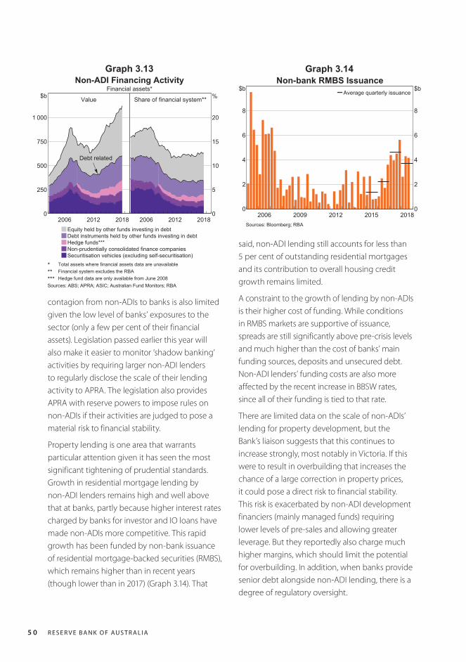
R E S E R V E B A N K O F AU S T R A L I A5 0
contagion from non-ADIs to banks is also limited given the low level of banks’ exposures to the sector (only a few per cent of their financial assets). Legislation passed earlier this year will also make it easier to monitor ‘shadow banking’ activities by requiring larger non-ADI lenders to regularly disclose the scale of their lending activity to APRA. The legislation also provides APRA with reserve powers to impose rules on non-ADIs if their activities are judged to pose a material risk to financial stability.
Property lending is one area that warrants particular attention given it has seen the most significant tightening of prudential standards. Growth in residential mortgage lending by non-ADI lenders remains high and well above that at banks, partly because higher interest rates charged by banks for investor and IO loans have made non-ADIs more competitive. This rapid growth has been funded by non-bank issuance of residential mortgage-backed securities (RMBS), which remains higher than in recent years (though lower than in 2017) (Graph 3.14). That
Graph 3.13Non-ADI Financing Activity
Financial assets*
Value
20122006 20180
250
500
750
1 000
$b
Debt related
Share of financial system**
20122006 20180
5
10
15
20
%
Equity held by other funds investing in debtDebt instruments held by other funds investing in debtHedge funds***Non-prudentially consolidated finance companiesSecuritisation vehicles (excluding self-securitisation)* Total assets where financial assets data are unavailable** Financial system excludes the RBA*** Hedge fund data are only available from June 2008
Sources: ABS; APRA; ASIC; Australian Fund Monitors; RBA
Graph 3.14
Average quarterly issuance
2015201220092006 20180
2
4
6
8
$b
0
2
4
6
8
$bNon-bank RMBS Issuance
Sources: Bloomberg; RBA
said, non-ADI lending still accounts for less than 5 per cent of outstanding residential mortgages and its contribution to overall housing credit growth remains limited.
A constraint to the growth of lending by non-ADIs is their higher cost of funding. While conditions in RMBS markets are supportive of issuance, spreads are still significantly above pre-crisis levels and much higher than the cost of banks’ main funding sources, deposits and unsecured debt. Non-ADI lenders’ funding costs are also more affected by the recent increase in BBSW rates, since all of their funding is tied to that rate.
There are limited data on the scale of non-ADIs’ lending for property development, but the Bank’s liaison suggests that this continues to increase strongly, most notably in Victoria. If this were to result in overbuilding that increases the chance of a large correction in property prices, it could pose a direct risk to financial stability. This risk is exacerbated by non-ADI development financiers (mainly managed funds) requiring lower levels of pre-sales and allowing greater leverage. But they reportedly also charge much higher margins, which should limit the potential for overbuilding. In addition, when banks provide senior debt alongside non-ADI lending, there is a degree of regulatory oversight.
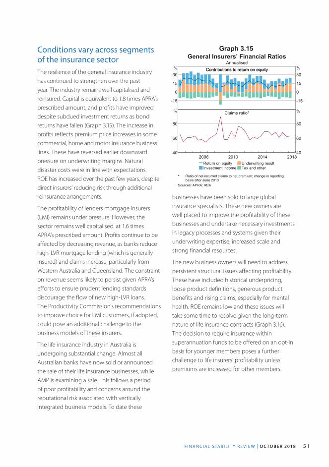
F I N A N C I A L S TA B I L I T Y R E V I E W | O C TO B E R 2018 5 1
Conditions vary across segments of the insurance sectorThe resilience of the general insurance industry has continued to strengthen over the past year. The industry remains well capitalised and reinsured. Capital is equivalent to 1.8 times APRA’s prescribed amount, and profits have improved despite subdued investment returns as bond returns have fallen (Graph 3.15). The increase in profits reflects premium price increases in some commercial, home and motor insurance business lines. These have reversed earlier downward pressure on underwriting margins. Natural disaster costs were in line with expectations. ROE has increased over the past few years, despite direct insurers’ reducing risk through additional reinsurance arrangements.
The profitability of lenders mortgage insurers (LMI) remains under pressure. However, the sector remains well capitalised, at 1.6 times APRA’s prescribed amount. Profits continue to be affected by decreasing revenue, as banks reduce high-LVR mortgage lending (which is generally insured) and claims increase, particularly from Western Australia and Queensland. The constraint on revenue seems likely to persist given APRA’s efforts to ensure prudent lending standards discourage the flow of new high-LVR loans. The Productivity Commission’s recommendations to improve choice for LMI customers, if adopted, could pose an additional challenge to the business models of these insurers.
The life insurance industry in Australia is undergoing substantial change. Almost all Australian banks have now sold or announced the sale of their life insurance businesses, while AMP is examining a sale. This follows a period of poor profitability and concerns around the reputational risk associated with vertically integrated business models. To date these
businesses have been sold to large global insurance specialists. These new owners are well placed to improve the profitability of these businesses and undertake necessary investments in legacy processes and systems given their underwriting expertise, increased scale and strong financial resources.
The new business owners will need to address persistent structural issues affecting profitability. These have included historical underpricing, loose product definitions, generous product benefits and rising claims, especially for mental health. ROE remains low and these issues will take some time to resolve given the long-term nature of life insurance contracts (Graph 3.16). The decision to require insurance within superannuation funds to be offered on an opt-in basis for younger members poses a further challenge to life insurers’ profitability unless premiums are increased for other members.
Graph 3.15General Insurers’ Financial Ratios
AnnualisedContributions to return on equityContributions to return on equity
-15
0
15
30%
-15
0
15
30%
Claims ratio*
201420102006 201840
60
80
%
40
60
80
%
Return on equityInvestment income
Underwriting resultTax and other
* Ratio of net incurred claims to net premium; change in reportingbasis after June 2010
Sources: APRA; RBA
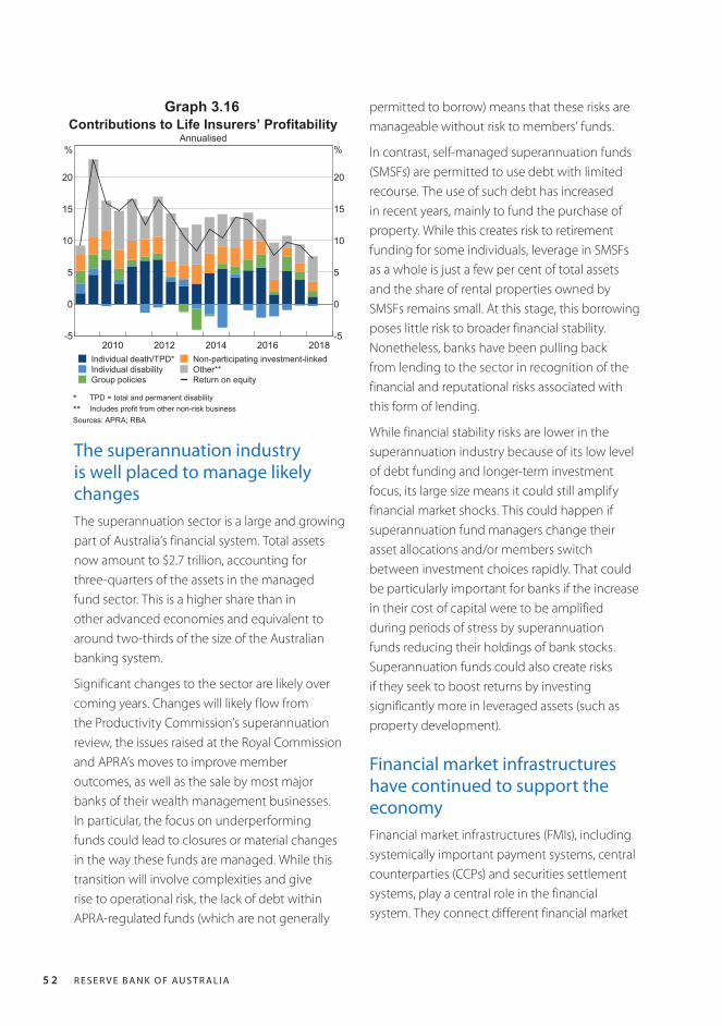
R E S E R V E B A N K O F AU S T R A L I A5 2
The superannuation industry is well placed to manage likely changesThe superannuation sector is a large and growing part of Australia’s financial system. Total assets now amount to $2.7 trillion, accounting for three-quarters of the assets in the managed fund sector. This is a higher share than in other advanced economies and equivalent to around two-thirds of the size of the Australian banking system.
Significant changes to the sector are likely over coming years. Changes will likely flow from the Productivity Commission’s superannuation review, the issues raised at the Royal Commission and APRA’s moves to improve member outcomes, as well as the sale by most major banks of their wealth management businesses. In particular, the focus on underperforming funds could lead to closures or material changes in the way these funds are managed. While this transition will involve complexities and give rise to operational risk, the lack of debt within APRA-regulated funds (which are not generally
permitted to borrow) means that these risks are manageable without risk to members’ funds.
In contrast, self-managed superannuation funds (SMSFs) are permitted to use debt with limited recourse. The use of such debt has increased in recent years, mainly to fund the purchase of property. While this creates risk to retirement funding for some individuals, leverage in SMSFs as a whole is just a few per cent of total assets and the share of rental properties owned by SMSFs remains small. At this stage, this borrowing poses little risk to broader financial stability. Nonetheless, banks have been pulling back from lending to the sector in recognition of the financial and reputational risks associated with this form of lending.
While financial stability risks are lower in the superannuation industry because of its low level of debt funding and longer-term investment focus, its large size means it could still amplify financial market shocks. This could happen if superannuation fund managers change their asset allocations and/or members switch between investment choices rapidly. That could be particularly important for banks if the increase in their cost of capital were to be amplified during periods of stress by superannuation funds reducing their holdings of bank stocks. Superannuation funds could also create risks if they seek to boost returns by investing significantly more in leveraged assets (such as property development).
Financial market infrastructures have continued to support the economyFinancial market infrastructures (FMIs), including systemically important payment systems, central counterparties (CCPs) and securities settlement systems, play a central role in the financial system. They connect different financial market
Graph 3.16
2016201420122010 2018-5
0
5
10
15
20
%
-5
0
5
10
15
20
%
Contributions to Life Insurers’ ProfitabilityAnnualised
Individual death/TPD*Individual disabilityGroup policies
Non-participating investment-linkedOther**Return on equity
* TPD = total and permanent disability** Includes profit from other non-risk businessSources: APRA; RBA
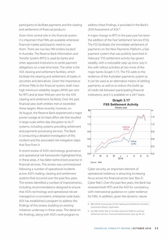
F I N A N C I A L S TA B I L I T Y R E V I E W | O C TO B E R 2018 5 3
participants to facilitate payments and the clearing and settlement of financial products.
Given their central role in the financial system it is important that FMIs are available whenever financial market participants need to use them. There are two key FMI entities located in Australia. The Reserve Bank Information and Transfer System (RITS) is used by banks and other approved institutions to settle payment obligations on a real-time basis. The other is the ASX clearing and settlement facilities, which facilitate the clearing and settlement of trades in securities and derivatives. Given the importance of these FMIs to the financial system, both have high minimum reliability targets (99.95 per cent for RITS and at least 99.8 per cent for the ASX clearing and settlement facilities). Over the past financial year, both entities met or exceeded these targets. More recently, however, on 30 August, the Reserve Bank experienced a major power outage at its head office site that resulted in large-scale within-day disruption to its IT systems, including systems providing settlement and payments processing services. The Bank is conducting a detailed investigation of this incident and the associated risk-mitigation steps that flow from it.
A recent review of ASX’s technology governance and operational risk frameworks highlighted that, in these areas, it has fallen behind best practice in financial services. This review was commissioned following a number of operational incidents across ASX’s trading, clearing and settlement systems that occurred over the past few years. The review identified a number of improvements, including recommendations designed to ensure that ASX’s technology and operational risk are managed on a consistent, enterprise-wide basis. ASX has established a program to address the findings of this review, building on existing initiatives underway in these areas. The detail on the findings, along with ASX’s work program to
address these findings, is provided in the Bank’s 2018 Assessment of ASX.8
A major change to RITS in the past year has been the addition of the Fast Settlement Service (FSS). The FSS facilitates the immediate settlement of payments on the New Payments Platform, a fast payment system that was publicly launched in February.9 FSS settlement activity has grown steadily, with a noticeable step-up since July in line with rollout activities at two more of the major banks (Graph 3.17). The FSS adds to the resilience of the Australian payments system as it can be used as an alternative means of settling payments, as well as to reduce the build-up of credit risk between participating financial institutions, and it is available on a 24/7 basis.
Cyber security, an important element of operational resilience, is attracting increasing focus across the financial sector (see ‘Box D: Cyber Risk’). Over the past few years, the Bank has reviewed both RITS and the ASX for consistency with international guidance on cyber resilience for FMIs. In addition, given the dynamic nature
8 RBA (2018), ‘Assessment of ASX Clearing and Settlement Facilities’, Assessment Report, September.
9 See RBA (2018), ‘Box D: The New Payments Platform and Fast Settlement Service’, Financial Stability Review, April, pp 49–52.
Graph 3.17
F M A M J J A S O2018
0.0
0.3
0.6
0.9
1.2
1.5
$b
0.0
0.3
0.6
0.9
1.2
1.5
m
FSS Settlement ActivityWeekly total
(LHS)Value
(RHS)Volume
Source: RBA
R E S E R V E B A N K O F AU S T R A L I A5 4
of cyber threats, the Bank has a program of ongoing work to strengthen RITS’ security controls and recovery planning. As part of this work RITS has recently undergone two external reviews, which assessed it as being compliant with all Society for Worldwide Interbank Finanical Telecommunication (SWIFT) mandatory security controls and with an international information security standard (ISO 27001).
While operational resilience is key for all FMIs, the role of CCPs is to manage financial risk. Given this, global standard setters have developed an international CCP workplan to promote CCP financial resilience, recovery planning and resolvability. The Bank uses the international guidance developed under this workplan in its supervision of CCPs. It has recently concluded an assessment of the ASX CCPs against the guidance and is in the process of assessing LCH Ltd’s SwapClear service. The Bank has concluded that ASX’s practices are consistent or broadly consistent with the international guidance, and ASX has a plan in place to address the gaps that have been identified. Further details are provided in the Bank’s 2018 Assessment of ASX. In addition to the work on CCP resilience and recovery arrangements, the Council of Financial Regulators agencies are developing a resolution regime for CCPs and other FMIs. R
F I N A N C I A L S TA B I L I T Y R E V I E W | O C TO B E R 2018 55
Box D
Cyber Risk
Over recent years regulators and financial institutions have increasingly focused on cyber risk. Cyber risk refers to the threat of financial losses, disruption and/or reputational damage from a malicious breach of an entity’s information systems. It is one component of operational (or technological) risk more broadly. The potential for cyber attacks is rising due to the growing use of information technology among businesses and consumers. The increasing presence and sophistication of cyber adversaries is also contributing to the growing threat.
Globally, the financial services and energy sectors account for the largest share of cyber incidents involving nationally important systems.1 The risk of cyber attacks in the financial system has increased due to a rapid rise in the digitalisation of services and use of third-party providers has increased the sector’s online footprint. Increased use of technology and digital records in banking, such as the introduction of open banking over the coming year, could raise additional cyber risks. As a result, cyber security will be a core challenge for the financial system for years to come.
There are different types of cyber attacksPerpetrators of cyber attacks are usually motivated by financial gains or a desire for notoriety. Malice can also be a driver. Attacks generally occur in one of four ways:
1 For an Australian perspective on this, see ACSC (2016), ‘Threat Report’, October. Available at <https://www.acsc.gov.au/publications/ACSC_Threat_Report_2016.pdf>.
• data breaches – where attackers aim to steal sensitive data. An example was an attack on Equifax where sensitive information from 147 million customers was obtained
• system disruptions – where attackers disrupt the availability of critical systems or websites, most commonly using a denial-of-service attack, such as during the 2016 Australian Census
• integrity of data attacks – when attackers modify information, often with the aim of rendering critical information unusable. Examples include the attack and release of altered medical records stored by the World Anti-Doping Agency in 2016
• financial attacks – where adversaries attack for financial gain and/or sabotage, either through fraud or ransom (often using ransomware). An example was the theft of US$81 million from Bangladesh Bank by an attack on their Society for Worldwide Interbank Financial Telecommunication (SWIFT) connected systems.
The incidence of cyber attack is risingThere is a lack of comprehensive data on cyber attack incidents or costs, in part because institutions and governments are reluctant to share this information. However, it is clear that financial institutions have increased their focus on cyber risk over recent years. One simple measure of this is that mentions of ‘cyber’ in the Australian major banks’ annual reports have risen
R E S E R V E B A N K O F AU S T R A L I A56
rapidly. Surveys of financial institutions show that cyber risk was considered one of the highest risks they faced in 2017, having not even been considered a top ten risk four years earlier.
There are some estimates of the extent of cyber attacks. An Accenture cybercrime report, based on a sample of 254 companies (across all industries) in seven advanced economies (including Australia), found a 27 per cent increase in successful breaches of company information security infrastructure in 2017 compared with a year earlier. This report also estimated that the average annual cost for each financial services entity to manage and recover from cyber attacks was US$18 million. The International Monetary Fund has estimated that direct losses from cyber attacks could be as large as 9 per cent of total bank net income globally.2 It estimated that this cost could rise to about one-third of income if the frequency of attacks and interconnectedness among institutions were to rise as per its ‘severe’ scenario. These estimates exclude indirect costs, such as the loss of reputation, which could make the potential losses even larger.
In Australia, no financial institution regulated by the Australian Prudential Regulation Authority (APRA) has yet recorded a significant financial or data loss from a cyber attack. However, half of the financial institutions surveyed by APRA in 2015/16 reported at least one cyber security incident that was material enough to report to executive management over the prior 12 months.
Some types of attacks could have financial stability impacts …Globally, successful cyber attacks have generally only affected a specific institution, but an attack could potentially spread to have systemic
2 Lagarde C (2018), ‘Estimating Cyber Risk for the Financial Sector’, IMF Blog, 22 June. Available at <https://blogs.imf.org/2018/06/22/estimating-cyber-risk-for-the-financial-sector/>.
implications. While the likelihood of an attack with severe financial stability implications is very low, the costs could be very large. The channels through which an attack on one institution could become systemic include operational dependencies (such as third-party providers), financial interconnectedness and the impact on confidence (including consumers and creditors).
The direct financial costs from a cyber attack can arise from fraud or ransom attacks and include the costs of lost data and/or the need to investigate and repair assets affected by the attack. However, it seems unlikely that an attack would have a large impact on the capital positions of Australia’s major banks.3 It is unlikely, for example, that a fraudulent attack that is large enough to directly threaten a bank’s viability could be disguised. Further, it is not credible to demand a ransom large enough to force a bank to fail.
A cyber attack that disrupts the payments system, particularly the wholesale payments network, could have more systemic implications. Disruption to the Reserve Bank Information and Transfer System (RITS) – which settles real-time high-value payments across Exchange Settlement Accounts held at the Reserve Bank – could prevent or delay a wide range of economic activity from occurring by stopping the final settlement of interbank payments. These include payments by governments (such as pensions and social security payments), corporations and between major banks and the Reserve Bank. Significant economic and financial stability consequences could develop if the disruption were not resolved in a timely manner.4 An outage of RITS could also result in a build-up of credit risk in the financial system until interbank obligations were settled.
3 These banks have around $170 billion in CET1 capital.4 International guidelines indicate that such systems should aim to be
operating again within two hours, and should complete settlement by the end of the day, even in extreme (but plausible) scenarios.
F I N A N C I A L S TA B I L I T Y R E V I E W | O C TO B E R 2018 57
… so supervisors and institutions are working to increase resilienceSupervisors and central banks globally have been increasing their focus on the growing threat from cyber attacks. The issue has been raised as a key risk in financial stability reports in numerous countries and is a focus for several international standard setters.
A key challenge for regulating cyber risk is accurately quantifying it, particularly given the rapidly evolving nature of cyber threats. Standard analytical tools cannot easily be used to quantify vulnerabilities, unlike in other parts of banks’ risk frameworks. In addition, cyber threats are dynamic in nature, meaning that current requirements may quickly become insufficient. For these reasons, regulators usually take a principles-based approach to regulating cyber threats.
The response by regulators to manage cyber risk varies and is at early stages compared with other risk frameworks (such as credit). A small number of jurisdictions have specific regulatory measures for managing cyber risks at banks, including Singapore, the United Kingdom and the United States.5 Cyber risk regulatory requirements in these jurisdictions are typically based on the framework set by the CPMI-IOSCO.6
This framework encourages entities to focus on strengthening five risk management categories: governance; identification; protection; detection; and response and recovery. It also encourages entities to continually test their systems and evolve their frameworks as key lessons are discovered. This requires firms to stay informed
5 For more information, see Crisanto J C and J Prenio (2017), ‘Regulatory approaches to enhance banks’ cyber-security frameworks’, FSI Insights on Policy Implementation No 2. Available at <https://www.bis.org/fsi/publ/insights2.pdf>.
6 The Committee on Payments and Market Infrastructure (CPMI) and the International Organization of Securities Commissions (IOSCO). While this framework was established for FMIs, its application is general enough to be extended to other financial institutions. For more details, see <https://www.bis.org/cpmi/publ/d146.pdf>.
A significant disruption to a retail payment system is likely to have a broad impact and could prevent customers from paying bills and/or transferring funds. This could create difficulties for some households. But unless it widely restricted access to, or damaged the perceived security of, deposits, it would be unlikely to adversely affect financial stability. The potential disruption caused by such an attack has risen as consumers have switched to digital payment methods, but cash is still a viable means of conducting most retail transactions.
A cyber attack involving a breach of data integrity in the financial system could have the most severe financial stability implications. For example, an attack that had implications for the integrity of banks’ record of their assets and liabilities could impede their ability to disburse funds to customers or collect on monies due. In the extreme it could raise questions about the institution’s solvency status. This could force directors to withdraw the bank from trading while investors may pull back on capital market funding.
Any type of material attack is also likely to have an impact on customers and creditors’ confidence that could amplify the shock. For example, there could be a marked deterioration in financial stability if creditors (both depositors and wholesale funders) lost confidence in the accessibility or security of the funds they have placed with banks. Australian banks could face liquidity issues if this resulted in creditors withdrawing funds or refusing to roll them over. In these circumstances, alternative funding sources would need to be accessed by banks, including as a last resort from the Reserve Bank’s liquidity provision mechanisms. A loss of confidence could also see consumers pull back from electronic transactions and towards cash.
R E S E R V E B A N K O F AU S T R A L I A58
and the Australian Securities and Investments Commission (ASIC) have powers to ensure that FMIs have effective controls to manage cyber threats and that they report cyber breaches to their supervisors in a timely manner. Indeed, cyber security has been a priority in the Reserve Bank’s supervision of FMIs and RITS in recent years. As part of this, the Reserve Bank recently reviewed the ASX against international guidance on cyber resilience, concluding that the ASX’s practices are consistent or broadly consistent with the guidance. A similar review of RITS in 2017 found no significant issues with its cyber security arrangements. As part of its continuous review of security practices, the Reserve Bank has in recent years made enhancements that further strengthen the resiliency of RITS to cyber attacks and its ability to recover from a successful attack within a short time frame. In recognition of this, RITS has recently been assessed as being compliant with various international standards. More broadly, ASIC has been strategically reviewing the cyber resilience of the financial sector firms it regulates, using standards-based surveillance tools, structured self-assessments and targeted interviews and follow ups.
The financial services sector is also responding to increasing cyber attack threats. SWIFT has introduced a ‘customer security program’ that establishes mandatory controls for security, guidelines for monitoring network breaches, and a protocol for sharing information on attacks. Private sector reports on cyber security also suggest that large financial institutions are investing heavily to strengthen defences against attacks. However, cyber security will need to continue to evolve as attackers increase their sophistication and ability. R
of developments in cyber security and to enhance their ability to pre-empt and manage cyber threats.
As supervisors strengthen guidance around cyber security, one consideration is ensuring that guidance is broadly harmonised across jurisdictions. In addition to reducing costs for banks that are active across several jurisdictions, harmonisation would recognise that cyber attacks affect financial institutions without regard to location and usually have cross-border implications. However, a mandated harmonised approach to cyber risk could also mean that vulnerabilities are common across countries and institutions. These issues are currently pertinent as over 70 per cent of supervisors expect to announce cyber security initiatives in the coming year.7
In Australia, APRA announced earlier this year that it will introduce its first prudential standard for information security management.8 Key objectives of the proposed prudential standard are for all APRA-regulated institutions and industries to maintain information security management controls that are commensurate with their size and the extent of the threat to information assets, and to have appropriate mechanisms in place to detect and respond to breaches in a timely manner. These principles-based proposed standards are expected to be finalised later this year and implemented by mid 2019.
Through their roles as supervisors of financial market infrastructures (FMIs), the Reserve Bank
7 See Financial Stability Board (2017), ‘Summary Report on Financial Cybersecurity Regulations, Guidance and Supervisory Practices’, October. Available at <http://www.fsb.org/2017/10/summary-report-on-financial-sector-cybersecurity-regulations-guidance-and-supervisory-practices/>.
8 For details, see APRA (2018), ‘APRA to introduce first prudential standard aimed at tackling growing threat of cyber attacks’, Media Release No 18.10, 7 March. Available at <https://www.apra.gov.au/media-centre/media-releases/apra-introduce-first-prudential-standard-aimed-tackling-growing-threat>.
F I N A N C I A L S TA B I L I T Y R E V I E W | O C TO B E R 2018 5 9
4. Regulatory Developments
At its recent meetings, the Council of Financial Regulators (CFR) continued its focus on risks stemming from housing lending. In particular, the CFR discussed and supported the decision by the Australian Prudential Regulation Authority (APRA) to begin to remove the investor loan benchmark. It considered several other areas of interest in recent meetings, including the ongoing work by APRA to develop a loss-absorbing capacity framework for Australian banks. The Reserve Bank of Australia (RBA) and other CFR agencies have been engaging extensively with the International Monetary Fund (IMF) as part of its Financial Sector Assessment Program (FSAP) review of Australia. The CFR has also been continuing its discussions on ways to enhance its transparency.
Internationally, the Financial Stability Board (FSB) and other global bodies have focused recently on two main tasks related to the post-crisis financial reforms. They have been assessing, and assisting, the implementation of key standards applying to the banking sector, and to global systemically important banks (G-SIBs) in particular. They have also been evaluating the effects of the reforms. Notably, the FSB published for consultation evaluations of the impact of the reforms on infrastructure finance and on incentives to centrally clear over-the-counter (OTC) derivatives.
Efforts to enhance or replace interest rate benchmarks are ongoing. This is important given concerns that existing key global benchmarks may not be sustainable. The RBA and the Australian Securities and Investments
Commission (ASIC) have worked with industry to enhance the robustness of the bank bill swap rate (BBSW), a key domestic interest rate benchmark. Financial technology, or ‘fintech’, has also remained on the agenda of many international and national bodies. Regulators recognise the potential benefits of innovation but remain alert to risks. A particular focus recently has been the potential risks posed by ‘crypto-assets’.
The CFR continues to be an effective coordinating bodyThe CFR is a forum for collaboration and coordination of Australia’s main financial regulatory agencies – APRA, ASIC, the RBA and the Australian Treasury. Its primary role is to contribute to the efficiency and effectiveness of financial regulation, and to promote the stability of the Australian financial system (see ‘Box E: The Council of Financial Regulators’). The CFR is supported by a number of inter-agency working groups, which conduct policy-related analysis and provide recommendations to the CFR as appropriate.
Over the past six months, the CFR has continued to closely monitor housing lending and the housing market. Discussions have covered mortgage lending practices, competition among different types of lenders, and the impact of various regulatory measures. This work has been supported by the Housing Market Risk Working Group, which provides analysis to the CFR on risks related to housing debt and potential policy options to limit these risks. In
R E S E R V E B A N K O F AU S T R A L I A6 0
April, following consultation with the CFR, APRA announced plans to remove the investor loan growth benchmark for authorised deposit-taking institutions (ADIs) that meet specific requirements (see the ‘Household and Business Finances’ chapter for further information). Relaxation of the benchmark has been made possible by more permanent measures to strengthen lending standards.
CFR members have also discussed options for the adoption of a loss-absorbing capacity (LAC) framework in Australia. LAC comprises internal resources that are intended to absorb losses and be used to support actions that help facilitate the orderly resolution of a distressed bank. APRA intends to release soon a discussion paper on a proposed approach for Australian banks for consultation.
The CFR also discussed a number of other issues at its meetings in June and September 2018, as noted below.
• APRA kept the CFR informed of its work on recovery and resolution planning. It provided an update on the outcome of its latest review of the recovery plans of large and medium-sized ADIs. These plans focus on the actions an ADI could take to respond to significant stress and restore itself to a financially sound position. APRA also provided an update on its resolution planning work for ADIs. Following the passing of the Financial Sector Legislation Amendment (Crisis Resolution Powers and Other Measures) Act 2018 earlier this year, APRA is working towards formalising its prudential framework for resolution over the coming years.
• The Climate Change Working Group provided an update on the work of CFR agencies to address climate-related risks to the financial system, highlighting in particular efforts to improve risk management and disclosure in
the sector. The Working Group noted that some meaningful change has already been observed among major institutions.
• The CFR began work on reviewing the regulatory arrangements for retail payment products. A particular focus is the arrangements for stored-value facilities, which were viewed by both the Financial System Inquiry and the Productivity Commission (PC) as complex and subject to potential regulatory overlap. An issues paper was released by the CFR in September to seek public input on the existing regulatory framework and possible approaches to reform.
• The CFR considered the final report of the PC’s inquiry into competition in the Australian financial system. Discussions focused on the recommendations related to the CFR – for instance, the inclusion of a ‘competition champion’ on the CFR and the release of CFR minutes – along with initial consideration of the PC’s other recommendations. CFR members supported the current composition of the CFR and arrangements for regular engagement with the Australian Competition and Consumer Commission (ACCC). They noted that the Treasury effectively played the role of ‘competition champion’. They also noted that the establishment of the ACCC’s Financial Services Unit had increased the level of engagement between individual CFR agencies and the ACCC on financial sector competition issues.
• Related to this, recognising the importance of transparency, the CFR considered possible approaches to further enhancing its external communications. The focus included finding the right balance between providing the public with an insight into the policy discussions at the CFR and maintaining confidentiality of sensitive regulatory
F I N A N C I A L S TA B I L I T Y R E V I E W | O C TO B E R 2018 6 1
matters. The approach to communications will also need to recognise that regulatory responsibilities rest with individual agencies, rather than the CFR itself. The CFR expects to provide information on any changes in its approach later in the year.
• The CFR also considered the issues that have arisen to date from the Royal Commission into Misconduct in the Banking, Superannuation and Financial Services Industry, along with cyber security risks and developments.
In addition to its regular meetings and agendas, the CFR engages with other regulatory bodies as appropriate to discuss issues of common interest.
• In 2017, the CFR held its first scheduled meeting with a broad group of domestic agencies that have an interest in financial sector developments. The second of these annual meetings was held in June 2018, involving the ACCC, the Australian Taxation Office and the Australian Transaction Reports and Analysis Centre (AUSTRAC). Topics discussed included the implications of recent reports and inquiries related to the financial sector, along with developments in distributed ledger technology (DLT) and its regulation.
• CFR agencies continued to work with their New Zealand counterparts via the Trans-Tasman Council on Banking Supervision (TTBC) to further strengthen the cross-border crisis management framework. Most recently, the TTBC has been carrying out follow-up work to the cross-border crisis simulation conducted in September 2017.
• In September, the CFR met with representatives of the IMF to discuss the preliminary findings of its FSAP review of the Australian financial system and regulatory framework (see below).
The IMF’s FSAP review of Australia is underwayThe RBA and other CFR agencies have been working closely with the IMF as part of its 2018 FSAP review of Australia. The FSAP is conducted every five years or so in jurisdictions with systemically important financial sectors (Australia’s previous FSAP was in 2012). In addition to assessing financial sector vulnerabilities, the IMF is focusing on the overall framework for systemic risk oversight. The FSAP includes an assessment of Australia’s banking regulatory and supervisory framework and practices. It is also reviewing the regulation of financial market infrastructures (FMIs) and the insurance sector, along with crisis management arrangements and Australia’s anti-money laundering and counter-terrorism financing regime. The FSAP has also involved an extensive ‘top down’ banking sector stress testing exercise. The IMF FSAP team has conducted two sets of meetings in recent months with the RBA and other CFR agencies, other government bodies, regulated institutions such as banks, ratings agencies, research houses and other organisations in forming its views. The RBA and other CFR agencies have participated in almost 100 meetings with the IMF FSAP team. Reports covering the above topics are expected to be published by the IMF in early 2019.
Internationally, efforts continue to address risks posed by globally systemic banks …Work to address the risks posed by systemically important financial institutions (SIFIs) is ongoing. SIFIs are institutions whose size, complexity and/or interconnectedness means their distress could disrupt the broader financial system and the wider economy. One core G20 post-crisis reform aimed at addressing this ‘too-big-to-fail’ issue was to enhance resolution regimes – these
R E S E R V E B A N K O F AU S T R A L I A6 2
are the legal and operational arrangements for managing a failing institution. The FSB’s 2011 standard, the Key Attributes of Effective Resolution Regimes for Financial Institutions (Key Attributes) aims to ensure the orderly resolution of a SIFI in financial stress to limit wider contagion. Since that time, the FSB has been monitoring global implementation of the standard. In June, the FSB launched its third peer review of resolution regimes. This peer review is focusing on the implementation of the resolution planning standard set out in the Key Attributes and the guidance relating to banks.
The FSB has also recently released two documents to guide authorities in applying the Key Attributes to the G-SIBs. These aim to enhance regulators’ ability to manage an orderly resolution of a G-SIB, though it is important to note that these arrangements have not yet been tested in the resolution of a large or systemic bank.
• Principles on Bail-in Execution. With bail-in, a bank is effectively recapitalised by write-downs and/or conversion of specific liabilities into equity. This aims to minimise the impact of a G-SIB resolution on financial stability, by ensuring the continuity of critical functions, while avoiding costs for taxpayers. The guidance sets out principles for authorities to consider as they make bail-in resolution strategies operational. The principles cover a range of issues surrounding bail-ins, including: disclosures on the instruments and liabilities affected; valuations; and communications to creditors and the market at large.
• Funding Strategy Elements of an Implementable Resolution Plan. This covers the development of a resolution funding plan for G-SIBs. It describes the home authority’s strategy and actions that would be used to address liquidity
stress. Areas covered include: the ability of G-SIBs to monitor, report on and estimate their funding needs in resolution and execute the funding strategy; the development of resolution funding plans by authorities; and access to temporary public-sector backstop funding and ordinary central bank facilities.
Related to this, the FSB issued in 2015 a standard on G-SIBs’ total loss-absorbing capacity (TLAC). TLAC aims to ensure that G-SIBs have sufficient liabilities (or capacity) suitable for absorbing losses. The standard starts to come into force from 2019. The FSB is currently preparing a report on the extent to which jurisdictions have implemented the TLAC standard, as well as reviewing G-SIB issuance strategies and overall progress in meeting TLAC requirements. The report, due to be published in the first half of 2019, will seek to identify any technical issues or challenges relating to the implementation of TLAC.
In July, the Basel Committee on Banking Supervision (BCBS) issued revisions to the assessment methodology for identifying G-SIBs. This methodology is based on a wide range of indicators. These cover banks’ size, interconnectedness and complexity as well as available substitutes for their services, and their cross-border activity. The core methodology was largely unchanged but the BCBS agreed on several modifications. The main revisions include: extending consolidation to include insurance subsidiaries; introducing a new trading volume indicator (addressing substitutability); and measuring cross-border activity with new consolidated international banking statistics from the Bank for International Settlements. The changes are to be implemented by 2021 when the next review of the G-SIB assessment methodology is also due to be completed.
F I N A N C I A L S TA B I L I T Y R E V I E W | O C TO B E R 2018 6 3
… as well as the wider banking sectorFollowing the final agreement on Basel III capital reforms in late 2017, the BCBS is focusing more on monitoring the implementation of its post-crisis reforms and changes to banking standards. As part of its monitoring, the BCBS released several reports over the past six months:
• A progress report found that the implementation of Basel III reforms was advancing.
– All jurisdictions have risk-based capital rules, Liquidity Coverage Ratio regulations and capital conservation buffers in place. In addition, all jurisdictions home to G-SIBs have final rules in force regarding G-SIB requirements.
– Most jurisdictions now enforce the leverage ratio, and most have final rules in force for the countercyclical capital buffer and for domestic systemically important banks.
– Jurisdictions made progress in implementing a number of other standards, broadly in line with their implementation deadlines. This includes the Net Stable Funding Ratio.
• Only marginal progress was made over the past year on banks’ implementation of the Principles for Effective Risk Data Aggregation and Risk Reporting according to a progress report. These principles aim to enhance banks’ risk management by improving their recording and reporting of risks. The BCBS noted that implementing the required improvements is complex. It made additional recommendations to assist and promote further adoption of the principles.
The BCBS has also continued its work to enhance standards for the regulation and oversight of the
banking sector. In May, it issued a standard on the capital treatment for simple, transparent and comparable (STC) short-term securitisations. This standard provides guidance for banks acting as investors or sponsors of such securitisations. Also, the BCBS and the International Organization of Securities Commissions (IOSCO) issued criteria for identifying short-term STC securitisations. These build on earlier criteria for identifying STC securitisations issued by the BCBS and IOSCO in July 2015, and incorporate feedback from public consultation.
Evaluating the effects of reforms is a major ongoing focus of global bodiesThe FSB and other international bodies are continuing to evaluate the effects of the core post-crisis reforms. They aim to assess whether the reforms are meeting their intended objectives and identify any material unintended consequences that may warrant an adjustment to the current approach. Any adjustments arising from FSB-coordinated evaluations would be made by the body that issued the standard. This would be done in a way that does not compromise the original objectives of the reforms or the agreed level of resilience.
Two FSB-led evaluations are currently underway. The first is on the incentives for market participants to centrally clear OTC derivatives. The second is on the effects of the reforms on financial intermediation, initially focusing on the cost and availability of infrastructure finance. Early findings from both evaluations have been presented at recent G20 meetings, and final reports will be delivered to the G20 Summit later this year.
• OTC derivatives markets were a core area of post-crisis reforms and so an early focus for evaluation. The reforms in this area aimed to reduce systemic risk and make derivatives
R E S E R V E B A N K O F AU S T R A L I A6 4
markets safer, for example, by reducing complexity and improving transparency. Clearing standardised OTC derivatives through a central counterparty was seen as key to achieving these aims. Several reforms provided incentives to centrally clear, either directly or indirectly. The FSB and relevant standard-setting bodies released a consultation paper in July providing an initial assessment of how the post-crisis reforms interact and affect incentives to centrally clear.
– The changes observed in OTC derivatives markets were found to be consistent with the G20 aim of promoting central clearing, especially for the most systemic market participants. In particular, the capital, margin and clearing reforms combine to create an incentive to centrally clear OTC derivatives, at least for dealers and larger and more active clients. In addition, non-regulatory factors, such as market liquidity and counterparty credit risk management, can interact with regulatory factors to affect incentives to centrally clear. It was also found that the provision of client clearing services is concentrated in a relatively small number of bank-affiliated clearing firms. This can make access to central clearing difficult and costly for some smaller clients.
– One particular concern relates to the calculation of the Basel III leverage ratio. Initial margin paid by clients to a clearing service provider cannot be used by that provider to offset its potential future exposures when calculating its leverage ratio. Survey data indicate that this may be a disincentive for banks to offer or expand client clearing services. The consultation paper suggested that additional analysis would be useful to further assess these effects.
• Also in July, the FSB issued a consultation paper on the effects of financial regulatory reforms on infrastructure finance. The report focused on infrastructure finance that is provided in the form of corporate and project debt financing (loans and bonds). It noted that the effect of the G20 reforms on infrastructure finance is of a second order relative to other factors, such as the macrofinancial environment, government policy and institutional factors. It also noted that the analysis to date does not identify material negative effects of key reforms (such as Basel III) on the provision and cost of infrastructure finance.
The FSB has agreed on two new evaluations, to be launched in coming months. One will assess the effects of the reforms on the financing of small and medium-sized enterprises. This is part of the financial intermediation evaluation noted above, and is to be completed in 2019. The other evaluation will review the reforms addressing ‘too-big-to-fail’ and is to be completed in 2020.
Interest rate benchmarks are being enhanced and made more robust …Efforts to enhance the integrity of major interest rate benchmarks continue. These benchmarks, or reference rates, support the smooth functioning of the financial system. They are referenced in a wide range of financial contracts, including derivatives, loans and securities. In response to instances of manipulation in the past, reforms have focused on increasing the extent to which benchmark rates are based on actual transactions, and on developing benchmarks based on (near) risk-free rates. Risk-free rates are typically based on overnight interbank markets where there are large volumes of transactions
F I N A N C I A L S TA B I L I T Y R E V I E W | O C TO B E R 2018 6 5
by many participants. This makes them more difficult to manipulate and means that sufficient transactions to produce benchmark rates are available more consistently. The development and adoption of new benchmarks has become more important given questions about the sustainability of the London Interbank Offered Rate (LIBOR). LIBOR is the key benchmark interest rate for several major currencies, but there are too few transactions for its reliable calculation.
One issue with moving to new benchmark rates is that many existing financial contracts refer to existing benchmark rates, such as the US dollar (USD) LIBOR. Many of these contracts have ‘fallback’ clauses if LIBOR were to cease, but these would be cumbersome to apply and could lead to significant market disruption. To address this risk, the FSB has encouraged the International Swaps and Derivatives Association (ISDA) to work with market participants to develop a more suitable fallback methodology – using the risk-free rate benchmarks that have been identified in particular jurisdictions. In July, ISDA launched a consultation on technical issues related to new benchmark fallbacks for derivatives contracts in several major non-USD currencies, as well as the BBSW in Australia. The consultation sets out options for adjustments that would apply to the fallback rate in the event that one of these benchmarks was permanently discontinued. And, in September, ISDA released its ‘benchmarks supplement’, which gives firms the ability to improve the contractual robustness of derivatives that reference certain benchmarks. By including this supplement into the terms of their derivatives contracts, market participants will be able to ensure that a cessation or material change to a benchmark is taken into account in their contracts and specify the fallback arrangements that would apply.
The United States in particular has made progress on this front. As noted in the previous Review, the Federal Reserve Bank of New York began publishing three new benchmark rates in April. One of these, the secured overnight financing rate (SOFR), was recommended by the Alternative Reference Rates Committee (ARRC) as the alternative to USD LIBOR.1 To facilitate its adoption by market participants, the ARRC released guiding principles in July for referencing SOFR.
European bodies are also continuing to work on two fronts. First, they are seeking to identify an appropriate risk-free rate to replace a current benchmark (the euro overnight index average (EONIA)). Second, they are enhancing the robustness of another current euro benchmark rate (EURIBOR), as well as developing a possible replacement rate.
• In June, the European Central Bank announced the methodology for calculating its new unsecured overnight rate, which it plans to publish by October 2019. The new euro short-rerm rate (ESTER) will be based entirely on money market statistical reporting. It will complement existing benchmark rates and serve as a backstop reference rate. Related to this, in September, a working group of key European bodies recommended ESTER as the new risk-free rate for the euro. In particular, ESTER is recommended as a replacement for EONIA given that EONIA will not meet the criteria of the European Union’s benchmarks regulation when it comes into force in 2020.
• With only limited transactions by a limited number of contributors, it is proving difficult to base EURIBOR on actual transactions. In response, its administrator (the European Money Markets Institute (EMMI)) has developed a hybrid model for the EURIBOR
1 The ARRC is a public-private body convened by the US Federal Reserve.
R E S E R V E B A N K O F AU S T R A L I A6 6
that will combine transactions, related market data and expert judgement. Industry feedback received during a consultation showed broad support for EMMI’s proposal. EMMI recently undertook in-depth testing of the proposed methodology, with another consultation scheduled soon to provide further technical detail on the hybrid approach.
In Australia, the implementation of changes to a key benchmark rate is more advanced. Unlike LIBOR, Australia’s main interest rate benchmark (BBSW) is generated from a market (the bank bill market) where there are considered to be enough transactions to calculate a robust benchmark. Nonetheless, the RBA and ASIC have been working with industry over recent years to enhance the robustness and longevity of BBSW. A number of important steps have been taken in recent months. In May, the BBSW methodology was strengthened to enable the benchmark to be calculated directly from a wider set of market transactions. The new methodology involves calculating BBSW as the volume-weighted average price of bank bill transactions during the morning rate set window. Further, in June, ASIC published rules for benchmark administrators (which, in the case of BBSW, is the ASX) based on new powers contained in legislation passed earlier this year. While BBSW is expected to remain a robust benchmark, it is prudent for users of BBSW to also have fallback arrangements in place in the event that BBSW was to be permanently discontinued. To address this risk, BBSW was included in the ISDA consultation noted above on benchmark fallbacks, with the relevant fallback for BBSW being the cash rate published by the RBA.2
The new legislation also gave ASIC the power to compel submissions to a ‘significant benchmark’
2 For more information on interest rate benchmarks, and especially the new BBSW methodology, see Alim S and E Connolly (2018), ‘Interest Rate Benchmarks for the Australian Dollar’, RBA Bulletin, September.
in the rare circumstances where the benchmark would otherwise cease to be published. It has also made the manipulation of financial benchmarks an offence. This new regulatory framework has reduced the uncertainty that institutions faced when participating in the BBSW rate-setting process. The RBA has also been encouraging the industry to consider whether risk-free interest rate benchmarks (such as the cash rate) are more appropriate for some financial contracts than credit-based benchmarks.
… as part of broader work to address misconduct in the financial sectorEnhancing the resilience of interest rate benchmarks is part of broader international and national efforts to address misconduct within financial institutions. In May, the FSB issued a consultation document on recommendations for consistent national reporting of data on the use of compensation tools to address misconduct risk. This is part of its Workplan on Measures to Reduce Misconduct Risk. If implemented, the recommendations would enhance supervisory authorities’ capacity to consider and monitor the effectiveness of compensation tools and other mechanisms in addressing misconduct risk. The recommendations include: reporting on incentive and compensation systems, including training, promotion and disciplinary systems; the inclusion of conduct in individual goals, and the linking of performance ratings to compensation; and specifying how misconduct is identified.
Domestically, the Banking Executive Accountability Regime (BEAR) commenced on 1 July 2018 for large ADIs and will apply to other ADIs from 1 July 2019. As discussed in ‘The Australian Financial System’ chapter, the BEAR aims to enhance transparency and accountability in ADIs by ensuring that they are
F I N A N C I A L S TA B I L I T Y R E V I E W | O C TO B E R 2018 6 7
clear about who holds ultimate responsibility for each part or aspect of their business. It imposes certain obligations on ADIs and their ‘accountable persons’ (senior executives and directors). Under the BEAR, courts can impose civil penalties on ADIs for breaches of these obligations, while APRA now has strengthened powers to disqualify accountable persons when they fail to meet their obligations. The BEAR also seeks to ensure that accountable persons face appropriate incentives for long-term decision-making by imposing minimum deferred remuneration requirements. More broadly, the CFR agencies regularly monitor developments related to culture within financial institutions.
Fintech and crypto-assets are attracting ongoing regulatory attentionFintech continues to be closely watched by international bodies and national regulators. These efforts typically recognise the benefits of fintech such as increased financial inclusion, enhanced competition and increased efficiencies. However, there is also a need to manage risks as fintech grows. One type of fintech that has attracted particular interest by global bodies recently is crypto-assets (including what are sometimes referred to as cryptocurrencies and other digital tokens). In July, the FSB released a report detailing its work on crypto-assets, as well as that of standard-setting bodies. This work includes the following:
• The FSB concluded that crypto-assets do not pose a material risk to global financial stability at this time. However, there is a need to protect consumers and investors, and prevent their use for illicit activities such as money laundering. Given the speed of development of crypto-asset markets, the FSB, in collaboration with the Committee on
Payments and Market Infrastructures (CPMI), has developed a framework for monitoring the financial stability implications of crypto-asset markets. The FSB will monitor the size and growth of crypto-asset markets. It will also monitor the use of leverage and financial institution exposures to crypto-asset markets.
• Given its mandate, the CPMI has paid particular attention to innovations in payments. It has conducted work on the use of DLT in payment, clearing and settlement activities, and on central bank digital currencies (CBDCs). The CPMI’s current workplan for innovation includes analysing the use of digital currencies in wholesale settlement, including possible safety and efficiency considerations. This involves digital currencies where access is limited to a predefined group of users, in contrast to general purpose digital currencies which would be widely accessible. The workplan also includes monitoring of developments in CBDCs across a range of countries.
• IOSCO has established an initial coin offering (ICO) Consultation Network.3 This will provide a forum for members to discuss their experiences with ICOs and bring their concerns, including any cross-border issues, to the attention of fellow regulators. It is also developing a framework to help members address domestic and cross-border investor protection issues arising from ICOs.
The UK Financial Conduct Authority (FCA) recently announced, in collaboration with ASIC and several other regulators and related organisations, the creation of the Global Financial Innovation Network (GFIN). The network aims
3 An ICO is a form of fundraising, used by a business or individual, to raise capital online. ICOs generally operate by allowing investors to use crypto-assets to purchase ‘coins’ that may offer some entitlement to future services. The ICOs are often global offerings that can be created anonymously and/or accepted anonymously.
R E S E R V E B A N K O F AU S T R A L I A6 8
to provide a more efficient way for innovative firms to interact with regulators, helping them navigate between countries as they look to test and develop new ideas. It will also create a new framework for cooperation between financial services regulators on innovation-related topics, sharing different experiences and approaches. The network is especially relevant for emerging technologies and business models that have cross-border application. The GFIN follows on from the FCA’s proposal in February to create a global ‘regulatory sandbox’. This would enable businesses to test products, services and business models for a limited time while subject to less stringent regulatory requirements.
Domestically, the RBA has continued to monitor fintech developments, including via the CFR Working Group on Distributed Ledger Technology. This monitoring in part focuses on fintech innovations in critical areas, such as FMIs, to make sure any vulnerabilities are managed and relevant systems and firms are resilient. Notably, the ASX has announced that it is replacing its core system for clearing, settlement and other post-trade services with a new system that uses DLT. The ASX released in September its implementation plan for the replacement, following public consultation earlier in the year.
The RBA has concluded that, at this stage, fintech developments do not raise major issues for monetary policy, payments system policy or its financial stability mandate. However, as in other countries, and as noted above, there are issues related to consumer and investor protection, and money laundering. Other Australian regulators have taken action in recent months in relation to crypto-assets:
• Legislation came into force in April that requires digital currency exchange (DCE) services to register with AUSTRAC and have a program to identify, mitigate and manage
money laundering and terrorism financing risks. DCE providers exchange money (whether Australian or foreign currency) for digital currency (or vice versa).
• Also in April, ASIC received delegated powers from the ACCC in relation to crypto-assets.4 These powers enable ASIC to take action against misleading or deceptive conduct in the marketing or selling of ICOs, even if the ICO does not involve a financial product. R
4 ASIC has also issued guidance on crypto-assets, see ASIC (May 2018)Information Sheet 225: Initial coin offerings and crypto-currency.
F I N A N C I A L S TA B I L I T Y R E V I E W | O C TO B E R 2018 69
Box E
The Council of Financial Regulators
The Council of Financial Regulators (CFR) is the coordinating body for Australia’s main financial regulatory agencies. There are four members: the Australian Prudential Regulation Authority (APRA), the Australian Securities and Investments Commission (ASIC), the Reserve Bank of Australia (RBA) and the Australian Treasury. The Reserve Bank Governor chairs the CFR and the RBA provides secretariat support. The CFR’s objectives, as set out in its Charter, are to contribute to the efficiency and effectiveness of financial regulation, and to promote stability of the Australian financial system.1
The CFR is a non-statutory body, unlike similar bodies in the United Kingdom and the United States. It does not have regulatory or policy decision-making powers of its own. Those powers reside with its members under their respective legislation. Instead, the CFR operates as a means for cooperation and coordination among member agencies. This box discusses the origins, processes and functions of the CFR.
History and governanceThe CFR was established in 1998 as the successor to the Council of Financial Supervisors (CFS), which had been in operation from 1992. The CFR’s collaborative, non-statutory structure was recommended by the 1997 report of the Financial System Inquiry (Wallis Committee). The Wallis Committee did not favour creating a statutory charter for the CFR as this could suggest that the CFR had regulatory functions
1 The Charter is available on the CFR’s website <https://www.cfr.gov.au>.
separate from those of its members. Instead, the Wallis Committee argued that the CFR, as a replacement to the CFS, should have the aim of facilitating close cooperation among its members. It saw the CFR as the collaborative dimension of the regulatory agencies’ activity. It did not see the CFR as a separate body with the ability to force cooperation among regulatory agencies.
The CFR was originally established with only three members: APRA, ASIC and the RBA. In 2003, the Treasurer announced that the Australian Treasury would join the CFR. This followed major changes to Australia’s financial regulatory structure brought about by the recommendations of the Royal Commission into the failure of HIH Insurance. At that time, the CFR Charter was also revised to provide a stronger focus on stability issues, including the promotion of coordination arrangements between regulators for handling episodes of financial instability. In March 2004, the RBA began publishing a semi-annual Financial Stability Review. Alongside the RBA’s assessment of the state of the financial system, each Review discusses activities of the CFR.
The CFR meets quarterly, or more often if required. At these meetings the four member agencies share views and information, and discuss regulatory reforms or issues where responsibilities overlap. They also coordinate responses to any threats to financial stability. This provides a flexible approach to coordination among the main financial regulatory agencies. Where appropriate, the CFR also provides joint
R E S E R V E B A N K O F AU S T R A L I A70
advice to the Government on current regulatory issues. As the secretariat, the RBA works to ensure the CFR operates effectively and within its mandate. This includes liaising with members to determine the agenda for CFR meetings and reaching out to non-member government agencies for their participation as appropriate.
The CFR’s focus on cooperation and coordination between the agencies is supported by multiple Memorandums of Understanding (MoUs) and bilateral coordination arrangements between member agencies. The MoUs cover such matters as information sharing, prompt notification of any regulatory decisions likely to impact other agencies’ responsibilities, and consultation arrangements in the event of financial disturbances. Given the CFR’s central role in crisis management, a specific MoU on financial distress management was agreed by the CFR members in 2008. This close cooperation is complemented by the Secretary to the Treasury sitting on the Reserve Bank Board and APRA having representation on the Bank’s Payments System Board.
OrganisationThe CFR comprises two representatives – the agency head and another senior representative – from each of the four member agencies. For the RBA, these representatives are the Governor and the Assistant Governor (Financial System). For the other agencies they are: the Chairman and Executive General Manager (Policy and Advice Division), APRA; the Chair and a Commissioner, ASIC; and the Secretary to the Treasury and Deputy Secretary (Markets Group), Treasury. Agencies may invite other internal specialists to speak on particular topics if required. Other regulatory bodies, such as the Australian Competition and Consumer Commission (ACCC) and the Australian Transaction Reports and
Analysis Centre (AUSTRAC), are invited to attend discussions relevant to their respective mandates.
Between quarterly meetings, the work of the CFR is facilitated through various working groups (see Figure E1). These groups progress work on specific topics or policy reforms. They develop papers for discussion that may include working-group-level advice on whether the CFR should support a particular position. The working groups are established either on an ongoing or temporary basis. Typically, each working group carries out work based on an agreed terms of reference, which sets out the group’s scope of work, objectives and timeline. Groups usually consist of representatives from each of the four CFR agencies, though non-member agencies with appropriate expertise participate in some groups; both the ACCC and AUSTRAC are currently participating in CFR working groups.
Some of the activities of these working groups include the following:
• The Financial Market Infrastructure Steering Committee (FMI SC) monitors, coordinates and prioritises interagency policy work in relation to FMIs and ‘over-the-counter’ (OTC) derivatives market regulation. It also provides policy direction and options to the CFR. In 2017, the FMI SC coordinated a joint CFR-ACCC public consultation on possible implications of competition in the settlement of cash equities in Australia for the functioning of markets, financial stability and access. This consultation, as with all public consultations and related announcements by the CFR, are made available on the CFR website <http://www.cfr.gov.au>.
• The Crisis Management Working Group (CMWG) was established in 2006 to set out policies and cross-agency processes to ensure the effective management of distressed financial institutions. As part of
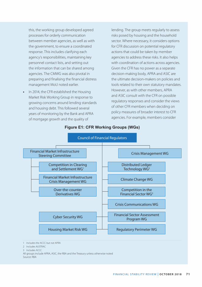
F I N A N C I A L S TA B I L I T Y R E V I E W | O C TO B E R 2018 71
this, the working group developed agreed processes for orderly communication between member agencies, as well as with the government, to ensure a coordinated response. This includes clarifying each agency’s responsibilities, maintaining key personnel contact lists, and setting out the information that can be shared among agencies. The CMWG was also pivotal in preparing and finalising the financial distress management MoU noted earlier.
• In 2014, the CFR established the Housing Market Risk Working Group in response to growing concerns around lending standards and housing debt. This followed several years of monitoring by the Bank and APRA of mortgage growth and the quality of
lending. The group meets regularly to assess risks posed by housing and the household sector. Where necessary, it considers options for CFR discussion on potential regulatory actions that could be taken by member agencies to address these risks. It also helps with coordination of actions across agencies. Given the CFR has no power as a separate decision-making body, APRA and ASIC are the ultimate decision-makers on policies and tools related to their own statutory mandates. However, as with other members, APRA and ASIC consult with the CFR on possible regulatory responses and consider the views of other CFR members when deciding on policy measures of broader interest to CFR agencies. For example, members consider
Council of Financial Regulators
Distributed Ledger Technology WG2
Climate Change WG
Cyber Security WG
Competition in the Financial Sector WG3
Crisis Communications WG
Financial Sector Assessment Program WG
Regulatory Perimeter WGHousing Market Risk WG
Figure E1: CFR Working Groups (WGs)
Financial Market Infrastructure Steering Committee Crisis Management WG
1 Includes the ACCC but not APRA2 Includes AUSTRAC3 Includes ACCCAll groups include APRA, ASIC, the RBA and the Treasury unless otherwise notedSource: RBA
Competition in Clearing and Settlement WG1
Financial Market Infrastructure Crisis Management WG
Over-the-counter Derivatives WG
R E S E R V E B A N K O F AU S T R A L I A72
the need to balance competition and stability when discussing possible policy actions.
Other working groups cover issues such as distributed ledger technology, competition, cyber security and the implications of climate change on the Australian financial system. A temporary working group is currently coordinating agency engagement with the International Monetary Fund as part of its Financial Sector Assessment Program (FSAP) review of Australia (for more information, see the ‘Regulatory Developments’ chapter).
Enhancing Australia’s crisis management arrangementsThe CFR also plays a central role in coordinating and advancing Australia’s framework for managing a major disruption to the financial system. This has included establishing arrangements to deal with potential threats to financial stability. Relevant examples include:
• In November 2005, the CFR advised the government on a package of measures for dealing with distressed financial institutions. This included the proposal for a Financial Claims Scheme (FCS) that would provide depositors in a failed authorised deposit-taking institution (ADI) and policyholders in a failed insurer with timely access to their funds up to a certain limit.
• In late 2008, the CFR played a critical role at the height of the global financial crisis, providing advice to the government on improving Australia’s crisis management arrangements. This included advice on the introduction of the FCS as well as a Guarantee Scheme for Large Deposits and Wholesale Funding. Both arrangements became operational in November 2008.
• At the request of the government, the CFR undertook an assessment in 2010 of whether the structure of the FCS was suitable for the post-crisis environment. Its advice informed the government’s revised arrangements for the FCS, including a lowering of the cap, which were subject to a public consultation process before their finalisation in 2011.
The CFR has also committed to regularly testing Australia’s crisis management framework, including the preparedness of the CFR to manage the failure of a financial institution. Crisis simulations are an effective means to test such arrangements and help identify areas that require further attention. In order to test cross-border arrangements, simulations are sometimes also carried out under the auspices of the Trans-Tasman Council on Banking Supervision (TTBC). The four CFR members are on the TTBC, along with the New Zealand Treasury, the Reserve Bank of New Zealand and the New Zealand Financial Markets Authority.
Accountability and membershipAs it does not determine or make policy, the CFR itself does not have explicit or formal accountability arrangements, beyond those already applying to its individual members. For example, all four agencies are subject to, and adhere to, the Public Governance, Performance and Accountability Act 2013. CFR members have been seeking ways to enhance the transparency of the CFR’s work. The CFR has a website and, starting from October 2017, each Financial Stability Review includes an expanded discussion of recent CFR activities. The final report of the Productivity Commission’s inquiry into competition in the Australian financial system also recommended the CFR further increase its transparency. The CFR is currently considering how this could best be achieved.

F I N A N C I A L S TA B I L I T Y R E V I E W | O C TO B E R 2018 73
The 2014 report of The Financial System Inquiry (Murray Committee) concluded no fundamental change to institutional arrangements related to financial stability policy was required. The Inquiry also concluded there was no need to expand the permanent membership of the CFR given other agencies attend meetings when appropriate. In contrast, more recently, the Productivity Commission recommended that membership be expanded to include the ACCC on the basis it could act as a ‘competition champion’. CFR members considered this recommendation, but concluded that the appropriate competition champion was the Treasury and that the CFR should continue to consult with the ACCC where appropriate. A separate annual meeting of CFR members and other regulatory agencies with an interest in the financial sector was instigated in 2017, including representatives of the ACCC, AUSTRAC and the Australian Taxation Office. R

R E S E R V E B A N K O F AU S T R A L I A74
F I N A N C I A L S TA B I L I T Y R E V I E W | O C TO B E R 2018 7 5
5. Assessing the Effects of Housing Lending Policy Measures
Since late 2014, regulators have implemented a suite of policy measures in an effort to mitigate the risks associated with certain forms of housing lending. The Australian Prudential Regulation Authority (APRA) imposed benchmarks on the lending of authorised deposit-taking institutions (ADIs) to investors and to borrowers taking out interest-only (IO) loans. APRA’s policy response also included measures to strengthen lending standards, with a greater focus on lending that involves higher risks, including high loan-to-valuation ratios (LVRs) and high debt-to-income lending. In addition, the Australian Securities and Investments Commission (ASIC) increased its scrutiny of lenders’ compliance with responsible lending obligations, with a particular focus on the appropriateness of IO lending.
Collectively, these measures have helped to reduce the riskiness of new borrowing. In turn, this has stemmed the increase in household sector vulnerabilities and improved the resilience of the economy to future shocks. The policy measures have required some borrowers and lenders to adjust their behaviour. However, there is little evidence to suggest that the measures have excessively constrained aggregate credit supply or had a significant impact on housing construction or competition for lending. This chapter outlines the policy measures and their impact on the riskiness of housing lending. It also presents quantitative analysis of the effect these measures have had on housing lending and the housing market more broadly.
Policy responded to the increase in housing debt vulnerabilities In 2014, a growing risk to household balance sheets was judged to be coming from the rapid increase in the share of housing lending to investors, alongside high housing debt that was rising considerably faster than incomes. This followed almost a decade in which household debt had grown broadly in line with income. The strong growth in investor borrowing when prices were rising rapidly was increasing the risk that investor activity could be excessively boosting housing prices and construction and so increasing the probability of a subsequent sharp unwinding. In turn, this constituted a downside risk for economic activity because highly indebted households could sharply reduce their consumption in the event of falls in incomes or house prices.1 An increase in higher risk and IO housing lending added to the concerns about household balance sheets. The regulatory measures implemented over several years sought to address these risks (Table 5.1). These measures were targeted at the risks surrounding housing lending, not at housing prices.
1 See, for example, RBA (2014), Financial Stability Review, September.
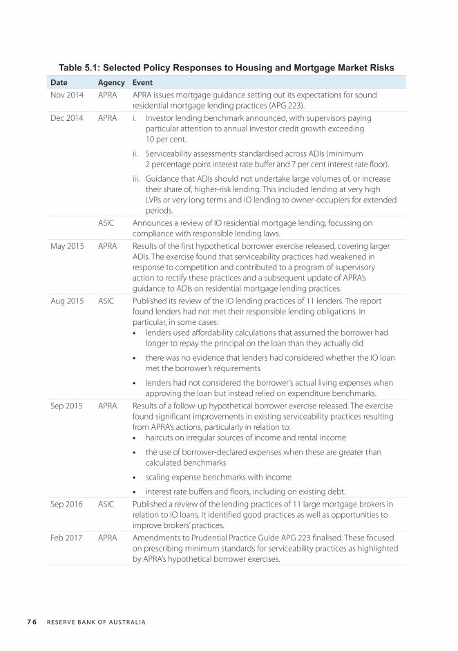
R E S E R V E B A N K O F AU S T R A L I A7 6
Date Agency EventNov 2014 APRA APRA issues mortgage guidance setting out its expectations for sound
residential mortgage lending practices (APG 223).Dec 2014 APRA i. Investor lending benchmark announced, with supervisors paying
particular attention to annual investor credit growth exceeding 10 per cent.
ii. Serviceability assessments standardised across ADIs (minimum 2 percentage point interest rate buffer and 7 per cent interest rate floor).
iii. Guidance that ADIs should not undertake large volumes of, or increase their share of, higher-risk lending. This included lending at very high LVRs or very long terms and IO lending to owner-occupiers for extended periods.
ASIC Announces a review of IO residential mortgage lending, focussing on compliance with responsible lending laws.
May 2015 APRA Results of the first hypothetical borrower exercise released, covering larger ADIs. The exercise found that serviceability practices had weakened in response to competition and contributed to a program of supervisory action to rectify these practices and a subsequent update of APRA’s guidance to ADIs on residential mortgage lending practices.
Aug 2015 ASIC Published its review of the IO lending practices of 11 lenders. The report found lenders had not met their responsible lending obligations. In particular, in some cases: • lenders used affordability calculations that assumed the borrower had
longer to repay the principal on the loan than they actually did
• there was no evidence that lenders had considered whether the IO loan met the borrower’s requirements
• lenders had not considered the borrower’s actual living expenses when approving the loan but instead relied on expenditure benchmarks.
Sep 2015 APRA Results of a follow-up hypothetical borrower exercise released. The exercise found significant improvements in existing serviceability practices resulting from APRA’s actions, particularly in relation to: • haircuts on irregular sources of income and rental income
• the use of borrower-declared expenses when these are greater than calculated benchmarks
• scaling expense benchmarks with income
• interest rate buffers and floors, including on existing debt.Sep 2016 ASIC Published a review of the lending practices of 11 large mortgage brokers in
relation to IO loans. It identified good practices as well as opportunities to improve brokers’ practices.
Feb 2017 APRA Amendments to Prudential Practice Guide APG 223 finalised. These focused on prescribing minimum standards for serviceability practices as highlighted by APRA’s hypothetical borrower exercises.
Table 5.1: Selected Policy Responses to Housing and Mortgage Market Risks
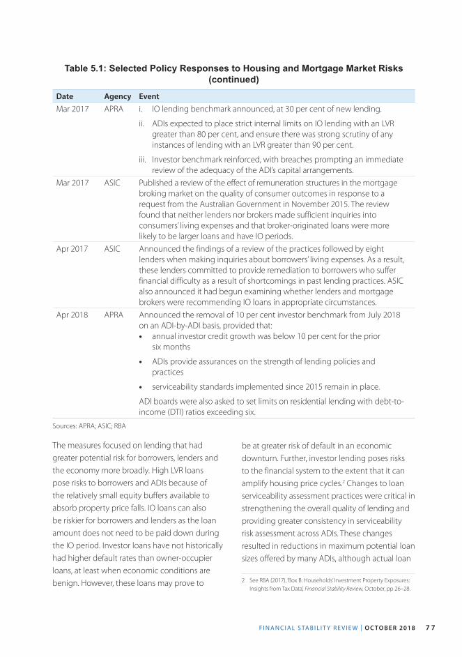
F I N A N C I A L S TA B I L I T Y R E V I E W | O C TO B E R 2018 7 7
Date Agency EventMar 2017 APRA i. IO lending benchmark announced, at 30 per cent of new lending.
ii. ADIs expected to place strict internal limits on IO lending with an LVR greater than 80 per cent, and ensure there was strong scrutiny of any instances of lending with an LVR greater than 90 per cent.
iii. Investor benchmark reinforced, with breaches prompting an immediate review of the adequacy of the ADI’s capital arrangements.
Mar 2017 ASIC Published a review of the effect of remuneration structures in the mortgage broking market on the quality of consumer outcomes in response to a request from the Australian Government in November 2015. The review found that neither lenders nor brokers made sufficient inquiries into consumers’ living expenses and that broker-originated loans were more likely to be larger loans and have IO periods.
Apr 2017 ASIC Announced the findings of a review of the practices followed by eight lenders when making inquiries about borrowers’ living expenses. As a result, these lenders committed to provide remediation to borrowers who suffer financial difficulty as a result of shortcomings in past lending practices. ASIC also announced it had begun examining whether lenders and mortgage brokers were recommending IO loans in appropriate circumstances.
Apr 2018 APRA Announced the removal of 10 per cent investor benchmark from July 2018 on an ADI-by-ADI basis, provided that: • annual investor credit growth was below 10 per cent for the prior
six months
• ADIs provide assurances on the strength of lending policies and practices
• serviceability standards implemented since 2015 remain in place.
ADI boards were also asked to set limits on residential lending with debt-to-income (DTI) ratios exceeding six.
Sources: APRA; ASIC; RBA
The measures focused on lending that had greater potential risk for borrowers, lenders and the economy more broadly. High LVR loans pose risks to borrowers and ADIs because of the relatively small equity buffers available to absorb property price falls. IO loans can also be riskier for borrowers and lenders as the loan amount does not need to be paid down during the IO period. Investor loans have not historically had higher default rates than owner-occupier loans, at least when economic conditions are benign. However, these loans may prove to
be at greater risk of default in an economic downturn. Further, investor lending poses risks to the financial system to the extent that it can amplify housing price cycles.2 Changes to loan serviceability assessment practices were critical in strengthening the overall quality of lending and providing greater consistency in serviceability risk assessment across ADIs. These changes resulted in reductions in maximum potential loan sizes offered by many ADIs, although actual loan
2 See RBA (2017), ‘Box B: Households’ Investment Property Exposures: Insights from Tax Data’, Financial Stability Review, October, pp 26–28.
Table 5.1: Selected Policy Responses to Housing and Mortgage Market Risks (continued)
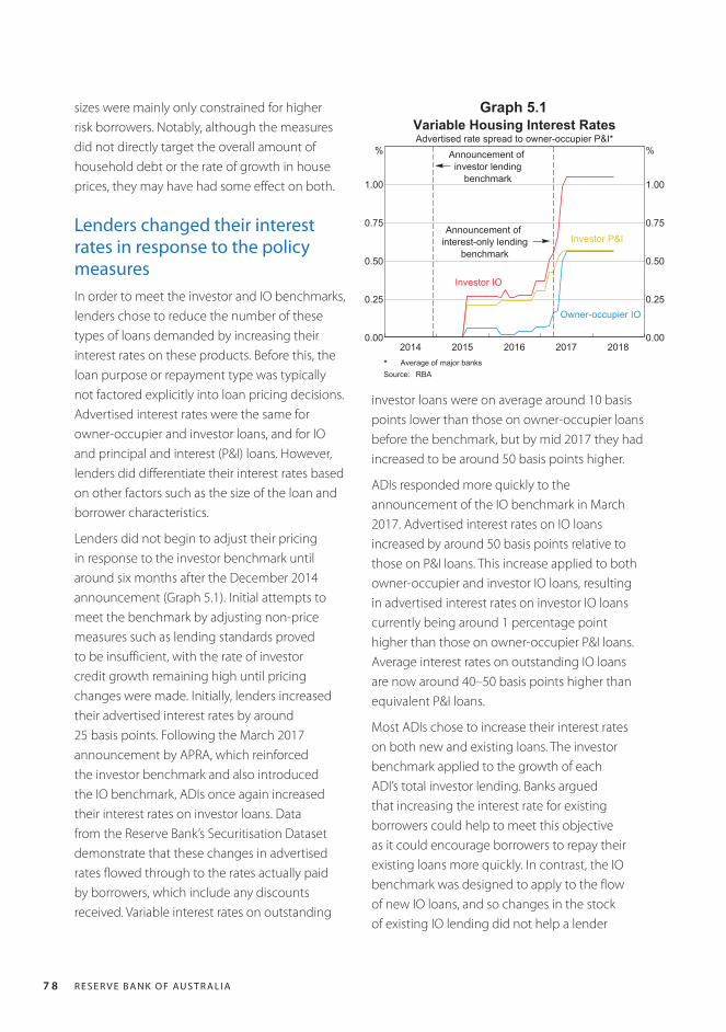
R E S E R V E B A N K O F AU S T R A L I A7 8
sizes were mainly only constrained for higher risk borrowers. Notably, although the measures did not directly target the overall amount of household debt or the rate of growth in house prices, they may have had some effect on both.
Lenders changed their interest rates in response to the policy measuresIn order to meet the investor and IO benchmarks, lenders chose to reduce the number of these types of loans demanded by increasing their interest rates on these products. Before this, the loan purpose or repayment type was typically not factored explicitly into loan pricing decisions. Advertised interest rates were the same for owner-occupier and investor loans, and for IO and principal and interest (P&I) loans. However, lenders did differentiate their interest rates based on other factors such as the size of the loan and borrower characteristics.
Lenders did not begin to adjust their pricing in response to the investor benchmark until around six months after the December 2014 announcement (Graph 5.1). Initial attempts to meet the benchmark by adjusting non-price measures such as lending standards proved to be insufficient, with the rate of investor credit growth remaining high until pricing changes were made. Initially, lenders increased their advertised interest rates by around 25 basis points. Following the March 2017 announcement by APRA, which reinforced the investor benchmark and also introduced the IO benchmark, ADIs once again increased their interest rates on investor loans. Data from the Reserve Bank’s Securitisation Dataset demonstrate that these changes in advertised rates flowed through to the rates actually paid by borrowers, which include any discounts received. Variable interest rates on outstanding
investor loans were on average around 10 basis points lower than those on owner-occupier loans before the benchmark, but by mid 2017 they had increased to be around 50 basis points higher.
ADIs responded more quickly to the announcement of the IO benchmark in March 2017. Advertised interest rates on IO loans increased by around 50 basis points relative to those on P&I loans. This increase applied to both owner-occupier and investor IO loans, resulting in advertised interest rates on investor IO loans currently being around 1 percentage point higher than those on owner-occupier P&I loans. Average interest rates on outstanding IO loans are now around 40–50 basis points higher than equivalent P&I loans.
Most ADIs chose to increase their interest rates on both new and existing loans. The investor benchmark applied to the growth of each ADI’s total investor lending. Banks argued that increasing the interest rate for existing borrowers could help to meet this objective as it could encourage borrowers to repay their existing loans more quickly. In contrast, the IO benchmark was designed to apply to the flow of new IO loans, and so changes in the stock of existing IO lending did not help a lender
2017201620152014 20180.00
0.25
0.50
0.75
1.00
%
0.00
0.25
0.50
0.75
1.00
%
Variable Housing Interest RatesAdvertised rate spread to owner-occupier P&I*
Investor IO
Investor P&I
Owner-occupier IO
Announcement ofinvestor lending
benchmark
Announcement ofinterest-only lending
benchmark
* Average of major banksSource: RBA
Graph 5.1
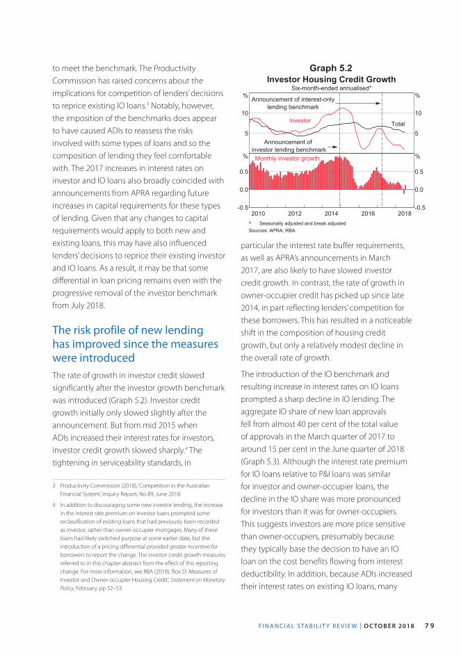
F I N A N C I A L S TA B I L I T Y R E V I E W | O C TO B E R 2018 7 9
to meet the benchmark. The Productivity Commission has raised concerns about the implications for competition of lenders’ decisions to reprice existing IO loans.3 Notably, however, the imposition of the benchmarks does appear to have caused ADIs to reassess the risks involved with some types of loans and so the composition of lending they feel comfortable with. The 2017 increases in interest rates on investor and IO loans also broadly coincided with announcements from APRA regarding future increases in capital requirements for these types of lending. Given that any changes to capital requirements would apply to both new and existing loans, this may have also influenced lenders’ decisions to reprice their existing investor and IO loans. As a result, it may be that some differential in loan pricing remains even with the progressive removal of the investor benchmark from July 2018.
The risk profile of new lending has improved since the measures were introducedThe rate of growth in investor credit slowed significantly after the investor growth benchmark was introduced (Graph 5.2). Investor credit growth initially only slowed slightly after the announcement. But from mid 2015 when ADIs increased their interest rates for investors, investor credit growth slowed sharply.4 The tightening in serviceability standards, in
3 Productivity Commission (2018), ‘Competition in the Australian Financial System’, Inquiry Report, No 89, June 2018.
4 In addition to discouraging some new investor lending, the increase in the interest rate premium on investor loans prompted some reclassification of existing loans that had previously been recorded as investor, rather than owner-occupier mortgages. Many of these loans had likely switched purpose at some earlier date, but the introduction of a pricing differential provided greater incentive for borrowers to report the change. The investor credit growth measures referred to in this chapter abstract from the effect of this reporting change. For more information, see RBA (2018), ‘Box D: Measures of Investor and Owner-occupier Housing Credit’, Statement on Monetary Policy, February, pp 52–53.
particular the interest rate buffer requirements, as well as APRA’s announcements in March 2017, are also likely to have slowed investor credit growth. In contrast, the rate of growth in owner-occupier credit has picked up since late 2014, in part reflecting lenders’ competition for these borrowers. This has resulted in a noticeable shift in the composition of housing credit growth, but only a relatively modest decline in the overall rate of growth.
The introduction of the IO benchmark and resulting increase in interest rates on IO loans prompted a sharp decline in IO lending. The aggregate IO share of new loan approvals fell from almost 40 per cent of the total value of approvals in the March quarter of 2017 to around 15 per cent in the June quarter of 2018 (Graph 5.3). Although the interest rate premium for IO loans relative to P&I loans was similar for investor and owner-occupier loans, the decline in the IO share was more pronounced for investors than it was for owner-occupiers. This suggests investors are more price sensitive than owner-occupiers, presumably because they typically base the decision to have an IO loan on the cost benefits flowing from interest deductibility. In addition, because ADIs increased their interest rates on existing IO loans, many
Investor Housing Credit GrowthSix-month-ended annualised*
5
10
%
5
10
%
Investor Total
Announcement ofinvestor lending benchmark
Announcement of interest-onlylending benchmark
2016201420122010 2018-0.5
0.0
0.5
%
-0.5
0.0
0.5
%Monthly investor growth
* Seasonally adjusted and break adjustedSources: APRA; RBA
Graph 5.2
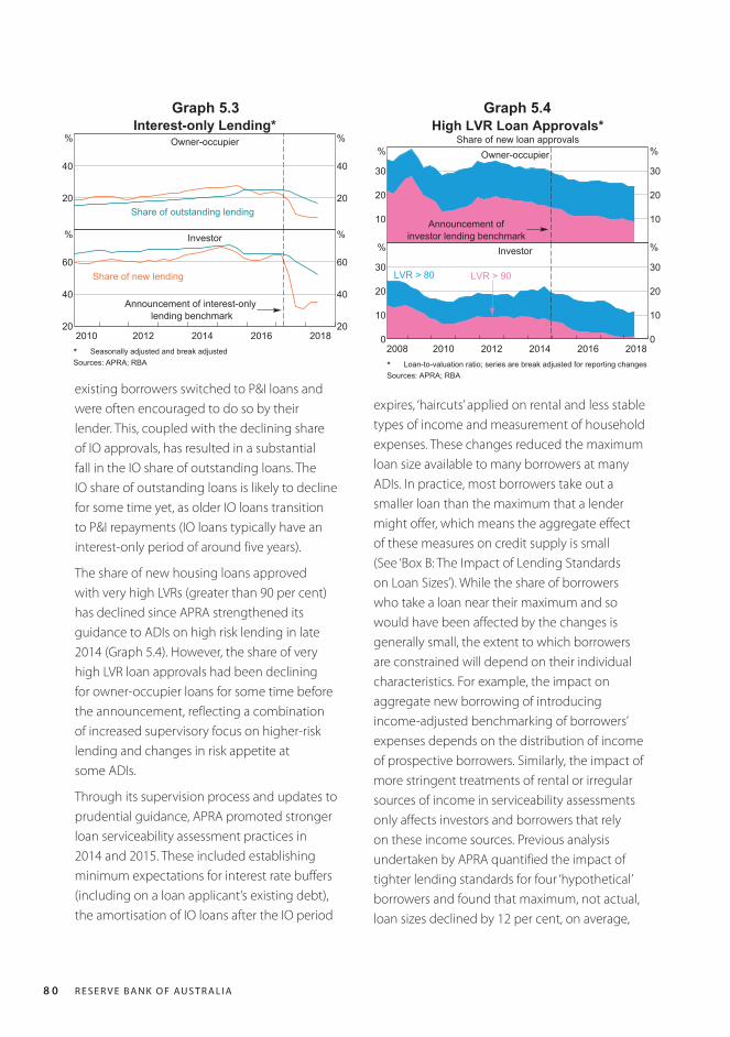
R E S E R V E B A N K O F AU S T R A L I A8 0
existing borrowers switched to P&I loans and were often encouraged to do so by their lender. This, coupled with the declining share of IO approvals, has resulted in a substantial fall in the IO share of outstanding loans. The IO share of outstanding loans is likely to decline for some time yet, as older IO loans transition to P&I repayments (IO loans typically have an interest-only period of around five years).
The share of new housing loans approved with very high LVRs (greater than 90 per cent) has declined since APRA strengthened its guidance to ADIs on high risk lending in late 2014 (Graph 5.4). However, the share of very high LVR loan approvals had been declining for owner-occupier loans for some time before the announcement, reflecting a combination of increased supervisory focus on higher-risk lending and changes in risk appetite at some ADIs.
Through its supervision process and updates to prudential guidance, APRA promoted stronger loan serviceability assessment practices in 2014 and 2015. These included establishing minimum expectations for interest rate buffers (including on a loan applicant’s existing debt), the amortisation of IO loans after the IO period
Interest-only Lending*Owner-occupier
20
40
%
20
40
%
Share of outstanding lending
Investor
2010 201620142012 201820
40
60
%
20
40
60
%
Share of new lending
Announcement of interest-onlylending benchmark
* Seasonally adjusted and break adjustedSources: APRA; RBA
Graph 5.3
expires, ‘haircuts’ applied on rental and less stable types of income and measurement of household expenses. These changes reduced the maximum loan size available to many borrowers at many ADIs. In practice, most borrowers take out a smaller loan than the maximum that a lender might offer, which means the aggregate effect of these measures on credit supply is small (See ‘Box B: The Impact of Lending Standards on Loan Sizes’). While the share of borrowers who take a loan near their maximum and so would have been affected by the changes is generally small, the extent to which borrowers are constrained will depend on their individual characteristics. For example, the impact on aggregate new borrowing of introducing income-adjusted benchmarking of borrowers’ expenses depends on the distribution of income of prospective borrowers. Similarly, the impact of more stringent treatments of rental or irregular sources of income in serviceability assessments only affects investors and borrowers that rely on these income sources. Previous analysis undertaken by APRA quantified the impact of tighter lending standards for four ‘hypothetical’ borrowers and found that maximum, not actual, loan sizes declined by 12 per cent, on average,
High LVR Loan Approvals*Share of new loan approvals
Owner-occupier
10
20
30
%
10
20
30
%
Announcement ofinvestor lending benchmark
Investor
2008 2016201420122010 20180
10
20
30
%
0
10
20
30
%
LVR > 90LVR > 80
* Loan-to-valuation ratio; series are break adjusted for reporting changesSources: APRA; RBA
Graph 5.4
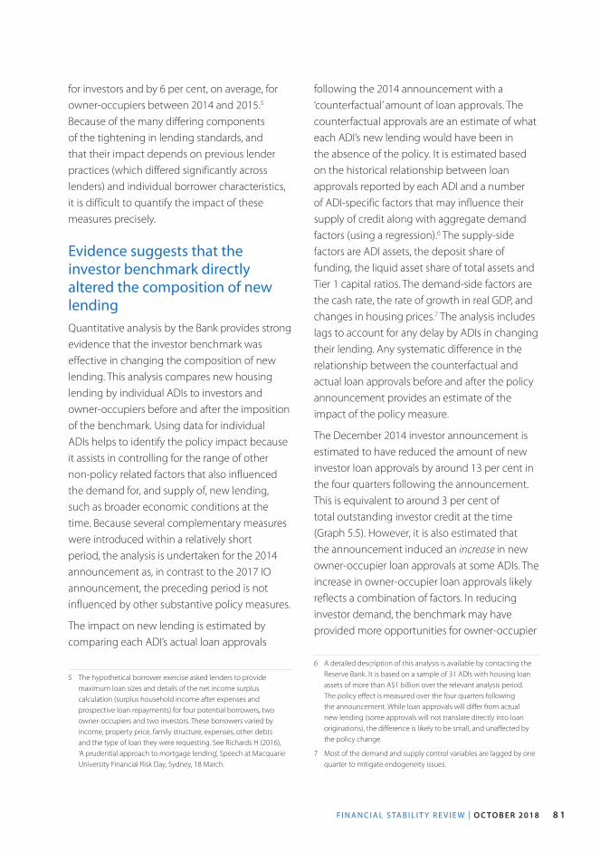
F I N A N C I A L S TA B I L I T Y R E V I E W | O C TO B E R 2018 8 1
for investors and by 6 per cent, on average, for owner-occupiers between 2014 and 2015.5 Because of the many differing components of the tightening in lending standards, and that their impact depends on previous lender practices (which differed significantly across lenders) and individual borrower characteristics, it is difficult to quantify the impact of these measures precisely.
Evidence suggests that the investor benchmark directly altered the composition of new lendingQuantitative analysis by the Bank provides strong evidence that the investor benchmark was effective in changing the composition of new lending. This analysis compares new housing lending by individual ADIs to investors and owner-occupiers before and after the imposition of the benchmark. Using data for individual ADIs helps to identify the policy impact because it assists in controlling for the range of other non-policy related factors that also influenced the demand for, and supply of, new lending, such as broader economic conditions at the time. Because several complementary measures were introduced within a relatively short period, the analysis is undertaken for the 2014 announcement as, in contrast to the 2017 IO announcement, the preceding period is not influenced by other substantive policy measures.
The impact on new lending is estimated by comparing each ADI’s actual loan approvals
5 The hypothetical borrower exercise asked lenders to provide maximum loan sizes and details of the net income surplus calculation (surplus household income after expenses and prospective loan repayments) for four potential borrowers, two owner-occupiers and two investors. These borrowers varied by income, property price, family structure, expenses, other debts and the type of loan they were requesting. See Richards H (2016), ‘A prudential approach to mortgage lending’, Speech at Macquarie University Financial Risk Day, Sydney, 18 March.
following the 2014 announcement with a ‘counterfactual’ amount of loan approvals. The counterfactual approvals are an estimate of what each ADI’s new lending would have been in the absence of the policy. It is estimated based on the historical relationship between loan approvals reported by each ADI and a number of ADI-specific factors that may influence their supply of credit along with aggregate demand factors (using a regression).6 The supply-side factors are ADI assets, the deposit share of funding, the liquid asset share of total assets and Tier 1 capital ratios. The demand-side factors are the cash rate, the rate of growth in real GDP, and changes in housing prices.7 The analysis includes lags to account for any delay by ADIs in changing their lending. Any systematic difference in the relationship between the counterfactual and actual loan approvals before and after the policy announcement provides an estimate of the impact of the policy measure.
The December 2014 investor announcement is estimated to have reduced the amount of new investor loan approvals by around 13 per cent in the four quarters following the announcement. This is equivalent to around 3 per cent of total outstanding investor credit at the time (Graph 5.5). However, it is also estimated that the announcement induced an increase in new owner-occupier loan approvals at some ADIs. The increase in owner-occupier loan approvals likely reflects a combination of factors. In reducing investor demand, the benchmark may have provided more opportunities for owner-occupier
6 A detailed description of this analysis is available by contacting the Reserve Bank. It is based on a sample of 31 ADIs with housing loan assets of more than A$1 billion over the relevant analysis period. The policy effect is measured over the four quarters following the announcement. While loan approvals will differ from actual new lending (some approvals will not translate directly into loan originations), the difference is likely to be small, and unaffected by the policy change.
7 Most of the demand and supply control variables are lagged by one quarter to mitigate endogeneity issues.
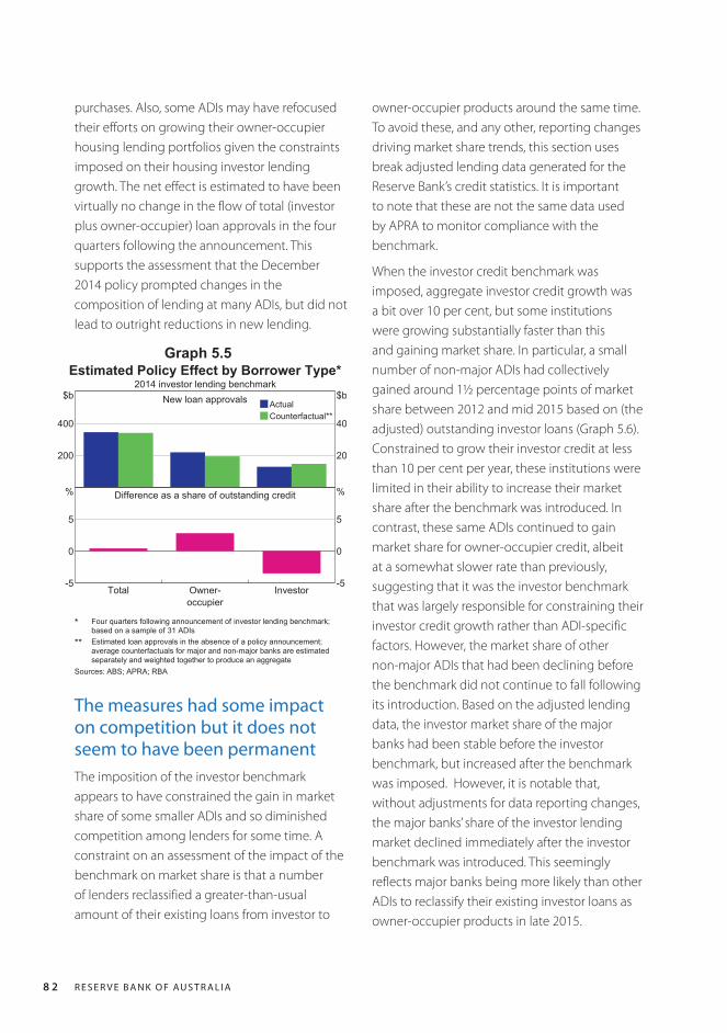
R E S E R V E B A N K O F AU S T R A L I A8 2
purchases. Also, some ADIs may have refocused their efforts on growing their owner-occupier housing lending portfolios given the constraints imposed on their housing investor lending growth. The net effect is estimated to have been virtually no change in the flow of total (investor plus owner-occupier) loan approvals in the four quarters following the announcement. This supports the assessment that the December 2014 policy prompted changes in the composition of lending at many ADIs, but did not lead to outright reductions in new lending.
Graph 5.5Estimated Policy Effect by Borrower Type*
2014 investor lending benchmarkNew loan approvals Actual
Counterfactual**
200
400
$b
200
400
$b
Difference as a share of outstanding credit
Total Owner-occupier
Investor-5
0
5
%
-5
0
5
%
* Four quarters following announcement of investor lending benchmark;based on a sample of 31 ADIs** Estimated loan approvals in the absence of a policy announcement;average counterfactuals for major and non-major banks are estimatedseparately and weighted together to produce an aggregate
Sources: ABS; APRA; RBA
The measures had some impact on competition but it does not seem to have been permanentThe imposition of the investor benchmark appears to have constrained the gain in market share of some smaller ADIs and so diminished competition among lenders for some time. A constraint on an assessment of the impact of the benchmark on market share is that a number of lenders reclassified a greater-than-usual amount of their existing loans from investor to
owner-occupier products around the same time. To avoid these, and any other, reporting changes driving market share trends, this section uses break adjusted lending data generated for the Reserve Bank’s credit statistics. It is important to note that these are not the same data used by APRA to monitor compliance with the benchmark.
When the investor credit benchmark was imposed, aggregate investor credit growth was a bit over 10 per cent, but some institutions were growing substantially faster than this and gaining market share. In particular, a small number of non-major ADIs had collectively gained around 1½ percentage points of market share between 2012 and mid 2015 based on (the adjusted) outstanding investor loans (Graph 5.6). Constrained to grow their investor credit at less than 10 per cent per year, these institutions were limited in their ability to increase their market share after the benchmark was introduced. In contrast, these same ADIs continued to gain market share for owner-occupier credit, albeit at a somewhat slower rate than previously, suggesting that it was the investor benchmark that was largely responsible for constraining their investor credit growth rather than ADI-specific factors. However, the market share of other non-major ADIs that had been declining before the benchmark did not continue to fall following its introduction. Based on the adjusted lending data, the investor market share of the major banks had been stable before the investor benchmark, but increased after the benchmark was imposed. However, it is notable that, without adjustments for data reporting changes, the major banks’ share of the investor lending market declined immediately after the investor benchmark was introduced. This seemingly reflects major banks being more likely than other ADIs to reclassify their existing investor loans as owner-occupier products in late 2015.
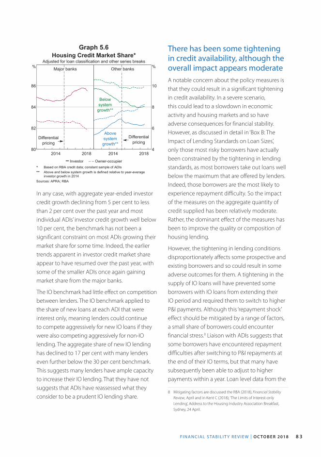
F I N A N C I A L S TA B I L I T Y R E V I E W | O C TO B E R 2018 8 3
Graph 5.6Housing Credit Market Share*
Adjusted for loan classification and other series breaks
Major banks
2014 201880
82
84
86
%
Differentialpricing
Other banks
2014 20184
6
8
10
%
Differentialpricing
Abovesystem
growth**
Belowsystem
growth**
Investor – – Owner-occupier* Based on RBA credit data; constant sample of ADIs** Above and below system growth is defined relative to year-averageinvestor growth in 2014
Sources: APRA; RBA
In any case, with aggregate year-ended investor credit growth declining from 5 per cent to less than 2 per cent over the past year and most individual ADIs’ investor credit growth well below 10 per cent, the benchmark has not been a significant constraint on most ADIs growing their market share for some time. Indeed, the earlier trends apparent in investor credit market share appear to have resumed over the past year, with some of the smaller ADIs once again gaining market share from the major banks.
The IO benchmark had little effect on competition between lenders. The IO benchmark applied to the share of new loans at each ADI that were interest only, meaning lenders could continue to compete aggressively for new IO loans if they were also competing aggressively for non-IO lending. The aggregate share of new IO lending has declined to 17 per cent with many lenders even further below the 30 per cent benchmark. This suggests many lenders have ample capacity to increase their IO lending. That they have not suggests that ADIs have reassessed what they consider to be a prudent IO lending share.
There has been some tightening in credit availability, although the overall impact appears moderate A notable concern about the policy measures is that they could result in a significant tightening in credit availability. In a severe scenario, this could lead to a slowdown in economic activity and housing markets and so have adverse consequences for financial stability. However, as discussed in detail in ‘Box B: The Impact of Lending Standards on Loan Sizes’, only those most risky borrowers have actually been constrained by the tightening in lending standards, as most borrowers take out loans well below the maximum that are offered by lenders. Indeed, those borrowers are the most likely to experience repayment difficulty. So the impact of the measures on the aggregate quantity of credit supplied has been relatively moderate. Rather, the dominant effect of the measures has been to improve the quality or composition of housing lending.
However, the tightening in lending conditions disproportionately affects some prospective and existing borrowers and so could result in some adverse outcomes for them. A tightening in the supply of IO loans will have prevented some borrowers with IO loans from extending their IO period and required them to switch to higher P&I payments. Although this ‘repayment shock’ effect should be mitigated by a range of factors, a small share of borrowers could encounter financial stress.8 Liaison with ADIs suggests that some borrowers have encountered repayment difficulties after switching to P&I repayments at the end of their IO terms, but that many have subsequently been able to adjust to higher payments within a year. Loan level data from the
8 Mitigating factors are discussed the RBA (2018), Financial Stability Review, April and in Kent C (2018), ‘The Limits of Interest-only Lending’, Address to the Housing Industry Association Breakfast, Sydney, 24 April.
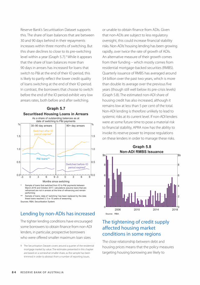
R E S E R V E B A N K O F AU S T R A L I A8 4
Reserve Bank’s Securitisation Dataset supports this. The share of loan balances that are between 30 and 90 days behind in their repayments increases within three months of switching. But this share declines to close to its pre-switching level within a year (Graph 5.7).9 While it appears that the share of loan balances more than 90 days in arrears has increased for loans that switch to P&I at the end of their IO period, this is likely to partly reflect the lower credit quality of loans switching at the end of their IO period. In contrast, the borrowers that choose to switch before the end of the IO period exhibit very low arrears rates, both before and after switching.
Lending by non-ADIs has increasedThe tighter lending conditions have encouraged some borrowers to obtain finance from non-ADI lenders, in particular, prospective borrowers who were offered smaller maximum loan sizes
9 The Securitisation Dataset covers around a quarter of the residential mortgage market by value. The estimates presented in this chapter are based on a somewhat smaller share, as the sample has been trimmed in order to abstract from a number of reporting issues.
Graph 5.7Securitised Housing Loans in Arrears
As a share of outstanding balances as atdate of switching to P&I payments
30–90 day arrears
-3 0 3 6 90.0
0.5
1.0
1.5
%
P&I loans**
Switched after IOperiod expired*
90+ day arrears
-3 0 3 6 90.0
0.5
1.0
1.5
%
Switched before IOperiod expired*
Months since switching* Sample of loans that switched from IO to P&I payments betweenMarch 2016 and October 2017; calculations assume loans that arerefinanced are not in arrears at the time of refinancing and remainperforming** Sample of loans; date of ‘switching’ has been replaced by the datethese loans reached 3, 5 or 10 years of seasoning
Sources: RBA; Securitisation System
or unable to obtain finance from ADIs. Given that non-ADIs are subject to less regulatory oversight, this could increase financial stability risks. Non-ADIs’ housing lending has been growing rapidly, over twice the rate of growth of ADIs. An alternative measure of their growth comes from their funding – which mostly comes from residential mortgage-backed securities (RMBS). Quarterly issuance of RMBS has averaged around $4 billion over the past two years, which is more than double its average over the previous five years (though still well below its pre-crisis levels) (Graph 5.8). The estimated non-ADI share of housing credit has also increased, although it remains low at less than 5 per cent of the total. Non-ADI lending is therefore unlikely to lead to systemic risks at its current level. If non-ADI lenders were at some future time to pose a material risk to financial stability, APRA now has the ability to invoke its reserve power to impose regulations on these lenders in order to manage these risks.
Graph 5.8
201420102006 20180
2
4
6
8
$b
0
2
4
6
8
$bNon-ADI RMBS Issuance
Source: RBA
The tightening of credit supply affected housing market conditions in some regionsThe close relationship between debt and housing prices means that the policy measures targeting housing borrowing are likely to
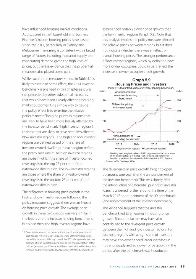
F I N A N C I A L S TA B I L I T Y R E V I E W | O C TO B E R 2018 8 5
have influenced housing market conditions. As discussed in the ‘Household and Business Finances’ chapter, housing prices have eased since late 2017, particularly in Sydney and Melbourne. The easing is consistent with a broad range of factors, including increased supply and moderating demand given the high level of prices, but there is evidence that the prudential measures also played some part.
While each of the measures set out in Table 5.1 is likely to have had some effect, the 2014 investor benchmark is analysed in this chapter as it was not preceded by other substantial measures that would have been already affecting housing market outcomes. One simple way to gauge the policy effect is to examine the relative performance of housing prices in regions that are likely to have been more heavily affected by the investor benchmark (‘high investor regions’) to those that are likely to have been less affected (‘low investor regions’). The high and low investor regions are defined based on the share of investor-owned dwellings in each region before the policy measure.10 The high investor regions are those in which the share of investor-owned dwellings is in the top 25 per cent of the nationwide distribution. The low investor regions are those where the share of investor-owned dwellings is in the bottom 25 per cent of the nationwide distribution.
The difference in housing price growth in the high and low investor regions following the policy measures suggests there was an impact on housing price growth. The average price growth in these two groups was very similar in the lead-up to the investor lending benchmark, but since then, the high investor regions have
10 Census data are used to calculate the share of rental properties in each region, which is taken to be the share of the dwelling stock owned by investors. Although dated, the 2011 data provide the best estimate of high investor regions prior to the implementation of the policies (whereas the 2016 data will have been affected by the policy measure and therefore not allow the policy effect to be identified).
experienced notably slower price growth than the low investor regions (Graph 5.9). Note that this analysis implies the policy measure affected the relative prices between regions, but it does not indicate whether there was an effect on overall housing prices. The stronger performance of low investor regions, which by definition have more owner-occupiers, could in part reflect the increase in owner-occupier credit growth.
Graph 5.9
201620142012 201880
90
100
110
120
index
80
90
100
110
120
index
Housing Prices and InvestorsIndex = 100 at introduction of investor lending benchmark
Differential pricingfor investor loans
Announcement ofinvestor lending benchmark
Announcement ofinterest-only lending
benchmark
High investor regions* Low investor regions*
* Dwelling stock weighted indices of SA3 regions where the rental shareof the dwelling stock is in the top (high investor) and bottom (lowinvestor) quartiles of the nationwide distribution in the 2011 Census
Sources: ABS; CoreLogic; RBA
The divergence in price growth began to open up around one year after the announcement of the investor benchmark. This was shortly after the introduction of differential pricing for investor loans. It widened further around the time of the March 2017 announcement of the IO benchmark (and reinforcement of the investor benchmark).
This evidence suggests that the investor benchmark led to an easing in housing price growth. But, other factors may have also contributed to the divergent price growth between the high and low investor regions. For example, regions with a high share of investors may have also experienced larger increases in housing supply and so slower price growth in the period after the benchmark was introduced.
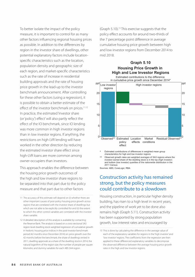
R E S E R V E B A N K O F AU S T R A L I A8 6
To better isolate the impact of the policy measure, it is important to control for as many other factors influencing regional housing prices as possible. In addition to the differences by region in the investor share of dwellings, other potential explanatory factors include location-specific characteristics such as the location, population density and geographic size of each region, and market-specific characteristics such as the rate of increase in residential building approvals and the rate of housing price growth in the lead-up to the investor benchmark announcement. After controlling for these other factors (using a regression), it is possible to obtain a better estimate of the effect of the investor benchmark on prices.11,12 In practice, the estimated ‘investor share (or ‘policy’) effect’ will also partly reflect the effect of the IO benchmark, since IO lending was more common in high investor regions than in low investor regions. If anything, the restrictions on high LVR lending will have worked in the other direction by reducing the estimated investor share effect since high-LVR loans are more common among owner-occupiers than investors.
This approach enables the difference between the housing price growth outcomes of the high and low investor share regions to be separated into that part due to the policy measure and that part due to other factors
11 The accuracy of this estimate will depend on (i) whether there are other important causes of post-policy housing price growth across regions that are correlated with the investor share of dwellings but which are not able to be explicitly controlled for and (ii) the extent to which the other control variables are correlated with the investor share variable.
12 A detailed description of this analysis is available by contacting the Reserve Bank. The analysis is based on a cross-sectional SA3 region-level dwelling stock weighted regression of cumulative growth in hedonic housing price indices in the post-investor benchmark period (42 months since December 2014) on: price growth over the 42 months before the benchmark; the share of dwellings rented in 2011; dwelling approvals as a share of the dwelling stock in 2014; the natural logarithm of the region size; the number of people per square kilometre; and dummy variables for each ABS SA4 region.
(Graph 5.10).13 This exercise suggests that the policy effect accounts for around two-thirds of the 7 percentage point difference in average cumulative housing price growth between high and low investor regions from December 2014 to mid 2018.
Construction activity has remained strong, but the policy measures could contribute to a slowdownHousing construction, in particular higher density building, has risen to a high level in recent years, and the pipeline of work yet to be done also remains high (Graph 5.11). Construction activity has been supported by strong population growth, low interest rates and encouraged by
13 This is done by calculating the difference in the average value of each of the explanatory variables for regions in the ‘high investor’ and ‘low investor’ regions. The coefficients from the regression are then applied to these differenced explanatory variables to decompose the observed difference between the average housing price growth rates in the high and low investor regions.
Graph 5.10Housing Price Growth in
High and Low Investor RegionsEstimated contributions to the difference
in cumulative price growth since December 2014*
Low investorregions
Observed**0
5
10
15
20
ppt High investor regions
Estimatedpolicyeffect
Locationeffects
Marketconditions
Residual Observed**0
5
10
15
20
ppt
* Estimated contributions of differences in weighted mean groupcharacteristics for high and low investor regions** Observed growth rates are weighted averages of SA3 regions where theinvestor-owned share of the dwelling stock is in the top (high investor)and bottom (low investor) quartiles of the nationwide distribution in the2011 Census
Sources: ABS; CoreLogic; RBA
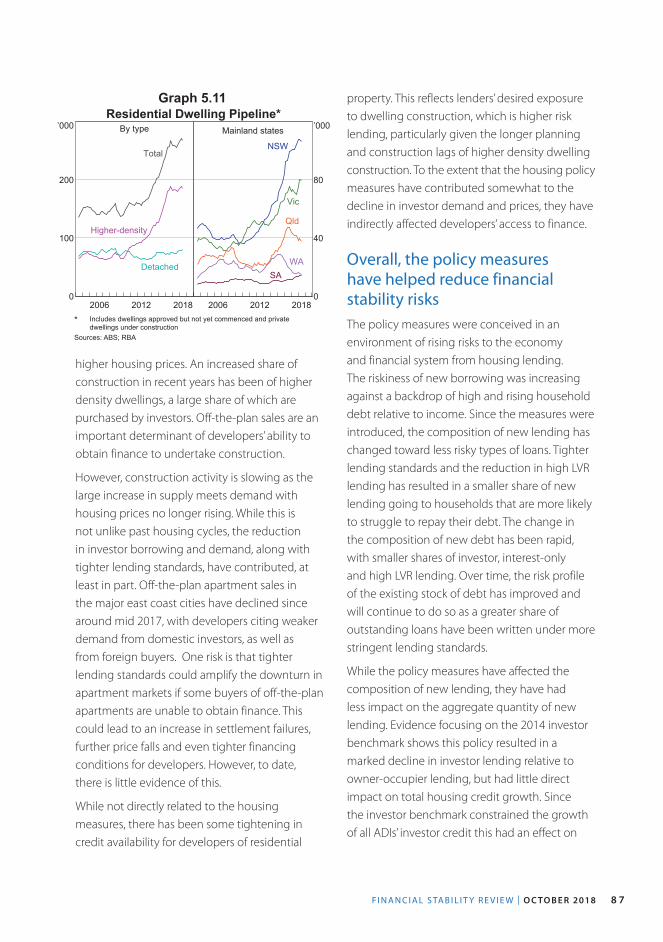
F I N A N C I A L S TA B I L I T Y R E V I E W | O C TO B E R 2018 8 7
property. This reflects lenders’ desired exposure to dwelling construction, which is higher risk lending, particularly given the longer planning and construction lags of higher density dwelling construction. To the extent that the housing policy measures have contributed somewhat to the decline in investor demand and prices, they have indirectly affected developers’ access to finance.
Overall, the policy measures have helped reduce financial stability risksThe policy measures were conceived in an environment of rising risks to the economy and financial system from housing lending. The riskiness of new borrowing was increasing against a backdrop of high and rising household debt relative to income. Since the measures were introduced, the composition of new lending has changed toward less risky types of loans. Tighter lending standards and the reduction in high LVR lending has resulted in a smaller share of new lending going to households that are more likely to struggle to repay their debt. The change in the composition of new debt has been rapid, with smaller shares of investor, interest-only and high LVR lending. Over time, the risk profile of the existing stock of debt has improved and will continue to do so as a greater share of outstanding loans have been written under more stringent lending standards.
While the policy measures have affected the composition of new lending, they have had less impact on the aggregate quantity of new lending. Evidence focusing on the 2014 investor benchmark shows this policy resulted in a marked decline in investor lending relative to owner-occupier lending, but had little direct impact on total housing credit growth. Since the investor benchmark constrained the growth of all ADIs’ investor credit this had an effect on
Graph 5.11Residential Dwelling Pipeline*
By type
20122006 20180
100
200
’000
Total
Higher-density
Detached
Mainland states
20122006 20180
40
80
’000
NSW
Vic
Qld
SAWA
* Includes dwellings approved but not yet commenced and privatedwellings under construction
Sources: ABS; RBA
higher housing prices. An increased share of construction in recent years has been of higher density dwellings, a large share of which are purchased by investors. Off-the-plan sales are an important determinant of developers’ ability to obtain finance to undertake construction.
However, construction activity is slowing as the large increase in supply meets demand with housing prices no longer rising. While this is not unlike past housing cycles, the reduction in investor borrowing and demand, along with tighter lending standards, have contributed, at least in part. Off-the-plan apartment sales in the major east coast cities have declined since around mid 2017, with developers citing weaker demand from domestic investors, as well as from foreign buyers. One risk is that tighter lending standards could amplify the downturn in apartment markets if some buyers of off-the-plan apartments are unable to obtain finance. This could lead to an increase in settlement failures, further price falls and even tighter financing conditions for developers. However, to date, there is little evidence of this.
While not directly related to the housing measures, there has been some tightening in credit availability for developers of residential
R E S E R V E B A N K O F AU S T R A L I A8 8
competition among lenders, but this does not appear to have been permanent. There is also evidence that, by affecting the composition of lending, the measures have influenced housing market conditions in those regions that were most affected by the change. In dampening investor demand, the measures are likely to have affected housing prices and construction dynamics in some locations, and so likely been stabilising for the housing market over the longer run. However, the measures have likely only had a moderate effect on aggregate housing prices given the evidence that at least the investor measure did not affect aggregate credit growth.
Overall, the available evidence suggests that the policies have meaningfully reduced vulnerabilities associated with riskier household lending and so increased the resilience of the economy to future shocks. However, the overall stock of household debt is high relative to income, suggesting that the associated risks remain. R
F I N A N C I A L S TA B I L I T Y R E V I E W | O C TO B E R 2018 8 9
Copyright and Disclaimer Notices
HILDAThe following Disclaimer applies to data obtained from the HILDA Survey and used in the chapter on ‘Household and Business Finances’ and reported in ‘Box B: The Impact of Lending Standards on Loan Sizes’ and ‘Box C: Vulnerable Households and Financial Stress’ in this issue of the Review.
Disclaimer
This Review uses unit record data from the Household, Income and Labour Dynamics in Australia (HILDA) Survey. The unit record data from the HILDA Survey was obtained from the Australian Data Archive, which is hosted by The Australian National University. The HILDA Survey was initiated and is funded by the Australian Government Department of Social Services (DSS) and is managed by the Melbourne Institute of Applied Economic and Social Research (Melbourne Institute). The findings and views reported in this Review, however, are those of the author and should not be attributed to the Australian Government, DSS, the Melbourne Institute, the Australian Data Archive or The Australian National University and none of those entities bears any responsibility for the analysis or interpretation of the unit record data from the HILDA Survey contained in this Review.

R E S E R V E B A N K O F AU S T R A L I A9 0