Financial Intermediation, House Prices, and the Welfare Effects of

the U.S. Great Recession∗

Dominik Menno† and Tommaso Oliviero‡

October 19, 2017

Abstract

This paper quantifies the welfare costs of the U.S. Great Recession and its distribution across

borrowing and saving households. We use a calibrated dynamic general equilibrium model with

shocks to aggregate income and to the financial intermediation sector. The model matches the

boom-bust cycle in house prices, the dynamics of household leverage, and the increase in wealth

inequality observed in the U.S. after 2007. We find large welfare costs of the Great Recession

for financially constrained households, the borrowers. Savers benefit from a redistribution of

housing wealth due to the de-leveraging of borrowers caused by falling house prices, which is

exacerbated by the financial intermediation shock. We also show the size of the welfare costs for

borrowers would have been lower if aggregate leverage would have remained at pre-2001 levels.

Keywords: Housing Wealth, Heterogeneous Agents, Welfare, Leverage

JEL Classification Numbers: D31, D58, D90, E21, E30, E44∗We thank Arpad Abraham, Alastair Ball, Almut Balleer, Christian Bayer, Alberto Bisin, Fabrice Collard, Antonia

Diaz, Marc Francke, Piero Gottardi, Nikolay Hristov, Thomas Hintermaier, Tim Kehoe, Sang Yoon (Tim) Lee, GuidoLorenzoni, Nicola Pavoni, Fabrizio Perri, Franck Portier, Sergio Rebelo, Victor Rios-Rull, Vincenzo Quadrini andseminar participants at the EUI Macro Working Group, the XVII Workshop on Dynamic Macro in Vigo 2012, theWorkshop on Institutions, Individual Behavior and Economic Outcomes in Argentiera 2012, the European Workshopin Macroeconomics 2013 at LSE, RWTH Aachen University 2012, Bocconi University 2012, University of Milan- Bicocca 2013, Federal Reserve Board of Governors 2013, the Ifo Institute Munich 2013, Bonn University 2013,the EEA Annual Congress in Gothenburg 2013, the Workshop on Macroeconomics, Financial Frictions and AssetPrices in Pavia 2013, the tenth CSEF-IGIER Symposium on Economics and Institutions in Capri 2014, Universityof Montreal 2014, Frankfurt-Mannheim-Macro-Workshop 2014, 7th ReCapNet Conference in Mannheim 2015, forhelpful comments on various drafts of this paper.†Corresponding author. Affiliation: Aarhus University. E-mail: dmenno@econ.au.dk‡Affiliation: University of Naples Federico II and CSEF, Italy. E-mail: tommaso.oliviero@unina.it

1

"When house prices in the aggregate collapse by 20 percent, the losses are concentrated on the

borrowers in the economy. [...] Given such a massive hit, the net worth of homeowners obviously

suffered. But what was the distribution of those losses: how worse off were borrowers actually?"

(Mian A. and Sufi A., House of Debt, University of Chicago Press, 2015)

1 Introduction

The U.S. Great Recession has been characterized by a large fall in GDP and an unprecedented

collapse of the housing market. The drop in aggregate house prices from 2007 onwards affected a

large number of U.S. households, potentially impacting on their consumption and, ultimately, their

welfare.1

During the last decade, the financial intermediation sector played a major role for the aggregate

dynamics of U.S. economy. First, the financial sector fueled funds to the U.S. households and

caused an unprecedented increase in aggregate leverage from the late 90’s.2 Second, the financial

intermediation sector has witnessed large short-run fluctuations in the last phase of the credit boom

(2004-2007), when financial innovation led to underpricing of credit risk and, after the start of the

financial crisis (2007-2010), when the large capital losses of intermediaries and the illiquidity in the

interbank market lowered the risk-bearing capacity of the banking sector.

These facts have stimulated the debate among economists and policy-makers on the distributive

impacts of the US Great Recession and on the role played by the financial intermediation sector.

This paper contributes to the literature by estimating the welfare costs of changes in the financial

intermediation sector on housing wealth and consumption of the U.S. households in the Great

Recession. In particular, we quantify to what extent the losses have been concentrated among

borrowing relative to saving households.1Iacoviello (2011) shows that housing wealth represents about half of total household net worth in 2008 and almost

two thirds of median household total wealth.2The literature has advocated different reasons behind the increase in the supply of credit such as the inflow of

foreign capital into the U.S. economy (Justiniano, Primiceri, and Tambalotti, 2014), the banking industry trends insecuritization practices which led to reduced lending standards(Brunnermeier, 2009; Dell’Ariccia, Igan, and Laeven,2012), and the rise in income inequality starting from the 80’s (Kumhof, Rancière, and Winant, 2015).

2

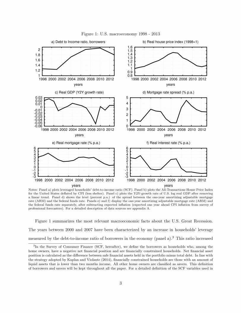
Figure 1: U.S. macroeconomy 1998 - 2013

1

1.2

1.4

1.6

1.8

2

1998 2000 2002 2004 2006 2008 2010 2012

years

a) Debt to Income ratio, borrowers

0.8 0.9

1 1.1 1.2 1.3 1.4 1.5 1.6

1998 2000 2002 2004 2006 2008 2010 2012

years

b) Real house price index (1998=1)

-0.06-0.05-0.04-0.03-0.02-0.01

0 0.01 0.02 0.03

1998 2000 2002 2004 2006 2008 2010 2012

years

c) Real GDP (Y2Y growth rate)

0

1

2

3

4

5

1998 2000 2002 2004 2006 2008 2010 2012

years

d) Mortgage rate spread (% p.a.)

-3-2-1 0 1 2 3 4 5 6

1998 2000 2002 2004 2006 2008 2010 2012

years

e) Real mortgage rate (% p.a.)

-3-2-1 0 1 2 3 4 5 6

1998 2000 2002 2004 2006 2008 2010 2012

years

f) Real interest rate (% p.a.)

Notes: Panel a) plots leveraged households’ debt-to-income ratio (SCF). Panel b) plots the All-Transactions House Price Indexfor the United States deflated by CPI (less shelter). Panel c) plots the Y2Y-growth rate of U.S. log real GDP after removinga linear trend. Panel d) shows the level (percent p.a.) of the spread between the one-year amortizing adjustable mortgagerate (ARM) and the federal funds rate. Panels e) and f) display the one-year amortizing adjustable mortgage rate (ARM) andthe federal funds rate separately, after subtracting expected inflation (expected one year ahead CPI inflation from survey ofprofessional forecasters). For a detailed description of data sources see appendix A.

Figure 1 summarizes the most relevant macroeconomic facts about the U.S. Great Recession.

The years between 2000 and 2007 have been characterized by an increase in households’ leverage

measured by the debt-to-income ratio of borrowers in the economy (panel a).3 This ratio increased3In the Survey of Consumer Finance (SCF, hereafter), we define the borrowers as households who, among the

home owners, have a negative net financial position and are financially constrained households. Net financial assetposition is calculated as the difference between safe financial assets held in the portfolio minus total debt. In line withthe strategy adopted by Kaplan and Violante (2014), financially constrained households are those with an amount ofliquid assets that is lower than two months income. All other home owners are classified as savers. This definitionof borrowers and savers will be kept throughout all the paper. For a detailed definition of the SCF variables used in

3

from about 1.2 in 2001 to a peak of more than 2 in 2010, and started to decline afterwards. The

increase in household leverage has been intertwined with an increase in house prices (panel b) of

about 30% between 2000-2006; this boom was followed by a quantitative similar drop after the

start of the Great Recession in 2007 when we observe a contemporaneous large drop in real GDP

of around 5.4% (panel c). Albuquerque, Baumann, and Krustev (2015) find that, different to

other recessions, the years following the Great Recession have been characterized by a reduction

in aggregate leverage, as observed in panel (a) from 2010 to 2013. We link such peculiarity of

this recession to the contemporaneous collapse of the financial market. The negative shock in the

financial intermediation sector is reflected by the increase of the mortgage rate spread after 2007

(panel d). The spread between the mortgage interest rate (panel e) and the federal funds rate

(panel f) reached a value of close to 0% between 2003 and 2006; in those years the interest rate on

mortgages remained stable despite the increase in the federal funds rate. Between 2007 and 2010,

however, the spread jumped to a level of about 4.5% and returned only slowly to pre-crisis levels in

subsequent years.4 When interpreting the dynamics of the mortgage rate spread, we share the view

of Gilchrist and Zakrajšek (2012) that the short-run increase and decrease of the spreads largely

reflect cyclical behavior in the risk-bearing capacity of the financial intermediation sector.

The dynamics of households’ leverage, house prices, GDP and spreads over the last decade nat-

urally raise the question of who bore the costs of this cycle. The collapse in house prices obviously

affected home owners. On the other hand, in line with the view of Mian and Sufi (2015), the welfare

losses from the aggregate collapse may have affected more the indebted home owners. Consistently

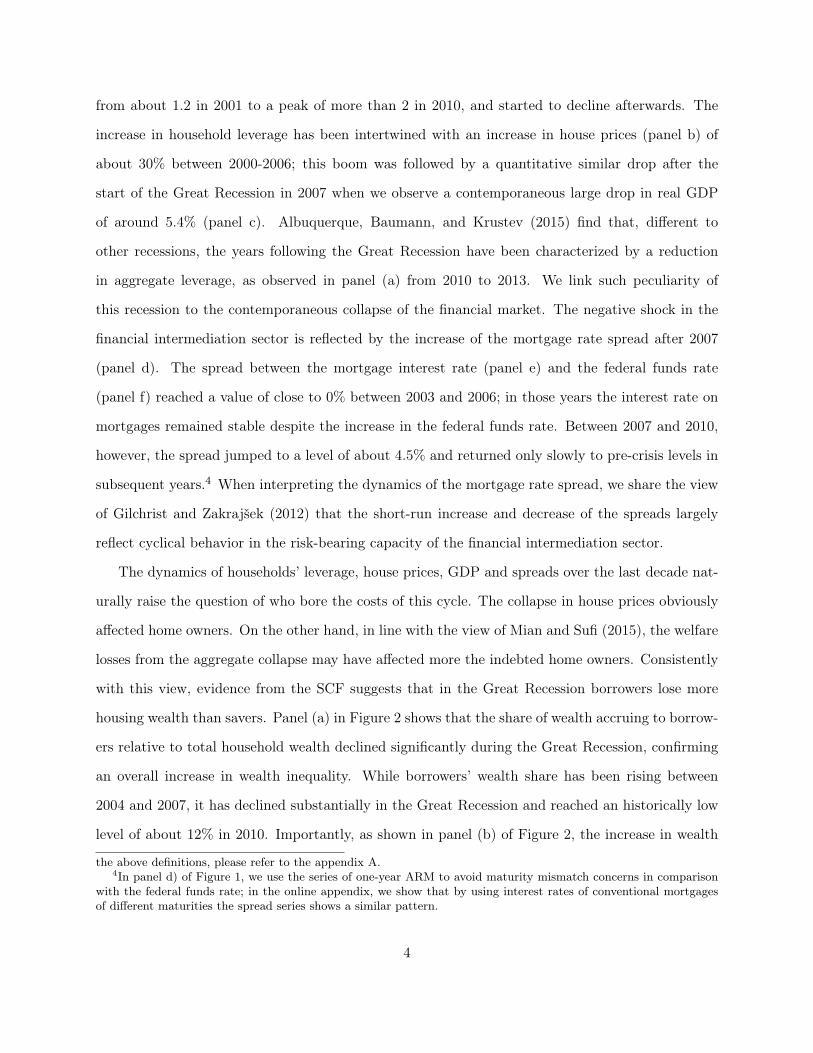
with this view, evidence from the SCF suggests that in the Great Recession borrowers lose more

housing wealth than savers. Panel (a) in Figure 2 shows that the share of wealth accruing to borrow-

ers relative to total household wealth declined significantly during the Great Recession, confirming

an overall increase in wealth inequality. While borrowers’ wealth share has been rising between

2004 and 2007, it has declined substantially in the Great Recession and reached an historically low

level of about 12% in 2010. Importantly, as shown in panel (b) of Figure 2, the increase in wealth

the above definitions, please refer to the appendix A.4In panel d) of Figure 1, we use the series of one-year ARM to avoid maturity mismatch concerns in comparison

with the federal funds rate; in the online appendix, we show that by using interest rates of conventional mortgagesof different maturities the spread series shows a similar pattern.

4

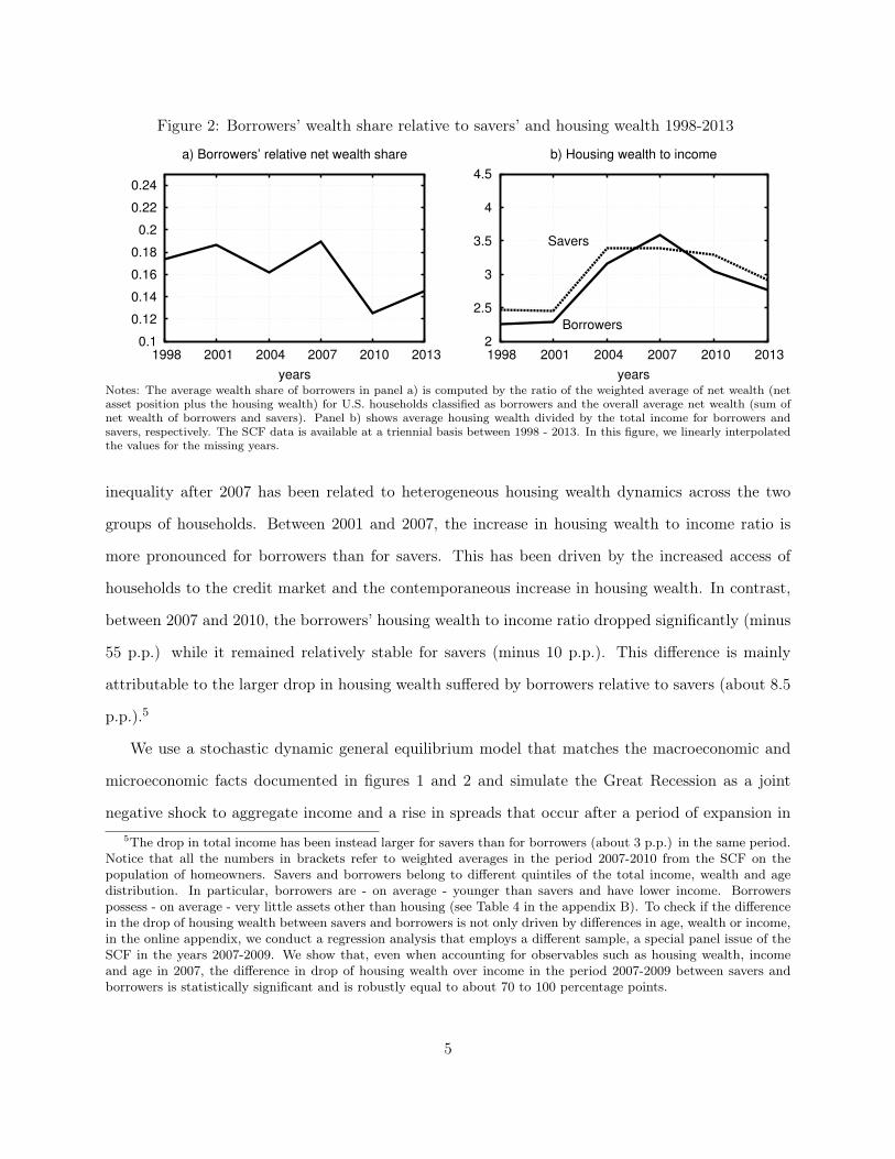
Figure 2: Borrowers’ wealth share relative to savers’ and housing wealth 1998-2013

0.1

0.12

0.14

0.16

0.18

0.2

0.22

0.24

1998 2001 2004 2007 2010 2013

years

a) Borrowers’ relative net wealth share

2

2.5

3

3.5

4

4.5

1998 2001 2004 2007 2010 2013

years

b) Housing wealth to income

Savers

Borrowers

Notes: The average wealth share of borrowers in panel a) is computed by the ratio of the weighted average of net wealth (netasset position plus the housing wealth) for U.S. households classified as borrowers and the overall average net wealth (sum ofnet wealth of borrowers and savers). Panel b) shows average housing wealth divided by the total income for borrowers andsavers, respectively. The SCF data is available at a triennial basis between 1998 - 2013. In this figure, we linearly interpolatedthe values for the missing years.

inequality after 2007 has been related to heterogeneous housing wealth dynamics across the two

groups of households. Between 2001 and 2007, the increase in housing wealth to income ratio is

more pronounced for borrowers than for savers. This has been driven by the increased access of

households to the credit market and the contemporaneous increase in housing wealth. In contrast,

between 2007 and 2010, the borrowers’ housing wealth to income ratio dropped significantly (minus

55 p.p.) while it remained relatively stable for savers (minus 10 p.p.). This difference is mainly

attributable to the larger drop in housing wealth suffered by borrowers relative to savers (about 8.5

p.p.).5

We use a stochastic dynamic general equilibrium model that matches the macroeconomic and

microeconomic facts documented in figures 1 and 2 and simulate the Great Recession as a joint

negative shock to aggregate income and a rise in spreads that occur after a period of expansion in5The drop in total income has been instead larger for savers than for borrowers (about 3 p.p.) in the same period.

Notice that all the numbers in brackets refer to weighted averages in the period 2007-2010 from the SCF on thepopulation of homeowners. Savers and borrowers belong to different quintiles of the total income, wealth and agedistribution. In particular, borrowers are - on average - younger than savers and have lower income. Borrowerspossess - on average - very little assets other than housing (see Table 4 in the appendix B). To check if the differencein the drop of housing wealth between savers and borrowers is not only driven by differences in age, wealth or income,in the online appendix, we conduct a regression analysis that employs a different sample, a special panel issue of theSCF in the years 2007-2009. We show that, even when accounting for observables such as housing wealth, incomeand age in 2007, the difference in drop of housing wealth over income in the period 2007-2009 between savers andborrowers is statistically significant and is robustly equal to about 70 to 100 percentage points.

5

household leverage. We use the model to study the dynamics of housing and non-durable consump-

tion to ultimately estimate their welfare implications. The model features heterogeneous households

and collateral constraints tied to housing wealth. In the model, households differ in their level of

patience, so that there are two types of households: borrowers - potentially financially constrained

- and savers. Agents are fully rational and derive utility from both the consumption of perishable

goods and of housing services coming from housing stock. Housing is the only physical asset in

the economy and it is fixed in supply.6 Borrowers collateralize debt by a fraction of their housing

wealth. Within this standard model, we introduce a competitive financial intermediation sector. All

saving and borrowing is conducted through this sector whose transformation technology, subject to

shocks, generates a time-varying spread between borrowing and lending rate.7 Financial intermedi-

ation shocks affect the amount of debt supplied to borrowers for a given level of aggregate savings

and collateral value. The second exogenous aggregate disturbance is a standard aggregate income

shock that affects the households’ endowment of the perishable good. It may be interpreted as a

reduced form way to capture the cyclical behavior of productivity shocks.

In order to study the transition towards high levels of households’ leverage and the subsequent

Great Recession, we introduce into the model a lending constraint that limits the total amount

of savings that is intermediated from savers to borrowers. In the spirit of Justiniano, Primiceri,

and Tambalotti (2015), a relaxation of this constraint captures the banking sector’s increase in

credit supply to the households that we observe in the data since the late 90’s. We calibrate the

model under the following two assumptions: (i) until the late 90’s, the U.S. economy was lending

constrained so that interest rates were high and aggregate mortgage debt was relatively low; (ii)

after 2001, the U.S. economy was no longer lending constrained and was converging towards a new

steady state where the households debt-to-income ratio was growing to historically high levels and,

at the same time, interest rates were falling. The presence of the lending constraint in the model

allows us to study one counterfactual scenario where we keep mortgage debt-to-income at pre-20016This assumption is motivated by the fact that before and during the Great Recession, house prices were most

volatile in geographical areas where the supply of houses was relatively fixed. See Figure IV in Mian and Sufi (2009).7We consider a simple model for the financial intermediation in the spirit of Cooper and Ejarque (2000) and

Cúrdia and Woodford (2010). Otherwise, the link to these studies is limited as the former looks at the business cycleproperties of financial shocks within a representative agent framework, while the latter studies the implications ofspread shocks for the optimal conduct of monetary policy.

6

levels (hence, there is no boom in debt-to-income) and feed into the simulated economy the same

shock sequence as observed in the Great Recession.

We highlight three main findings. First, borrowers suffer significantly more than savers in terms

of welfare from the Great Recession. Second, the negative financial intermediation shock, by directly

affecting the supply of debt to borrowers, generates a de-leveraging process even when the collateral

constraint is binding; the opposite is true for savers, who relatively benefit from the increase in

the mortgage spreads. Third, in the restricted lending counterfactual, we find the welfare effects of

financial intermediation shocks to be less (more) harmful for borrowers (savers). This finding points

to the combination of high pre-crisis leverage and the collapse in collateralized housing as the main

cause of the larger welfare loss for the leveraged households in the Great Recession.

The mechanism behind these findings is the following. A negative income shock leads to a

reduction in the aggregate demand for (both durable and non-durable) consumption goods and a

deflation pressure on house prices. The drop in the collateralized housing wealth generates a credit

contraction for borrowers who have access only to collateralized debt as a source of external financ-

ing. If the reduction is sufficiently large, the collateral constraint becomes binding and borrowers

reduce their housing stock. For a given supply of housing, house prices decrease further.8 Similarly,

savers suffer from the aggregate drop in house prices (negative wealth effect). However, given that

they are unconstrained and relatively more patient than borrowers and, given they expect house

prices to rise again in the future (shocks are mean-reverting in the model), they smooth their con-

sumption by buying houses when prices are low. The overall result of a negative income shock is

that both type of households suffer in terms of both wealth and expected lifetime utility, but the

welfare costs is significantly smaller for the savers.

When the income contraction is coupled with a negative financial intermediation shock, the

supply of loans to borrowers shrinks and they are forced to de-leverage by further selling the housing

stock at depreciated value to savers. This makes the housing wealth drop even larger, tightens the

collateral constraint further, and exacerbates the redistribution of the housing wealth from borrowers

to savers. Therefore, savers gain relatively more in terms of housing consumption and suffer less than8This mechanism is along the line of the debt-deflation mechanism in Bianchi and Mendoza (2010).

7

borrowers in terms of expected lifetime utility compared to a recession where financial intermediation

shocks do not occur. We finally show that the welfare impact of the financial intermediation shock,

resulting from the endogenous decline in households’ leverage, is larger the higher the level of

indebtedness when entering the recession.

The present study is related to different strands of the macroeconomic literature. First, this

paper relates to the recent literature that explores the effects of financial markets on the U.S.

macroeconomy in the Great Recession (Hall, 2011; Quadrini and Urban, 2012). Huo and Ríos-

Rull (2014) study the quantitative power of financial frictions in explaining the drop in housing

and stock prices; Justiniano, Primiceri, and Tambalotti (2015) highlight that credit supply shocks

played a pre-eminent role in qualitatively explaining the dynamics of house prices before and after

the Great Recession; although similar in spirit, our contribution is the focus on welfare implications

of changes in the financial intermediation sector. Guerrieri and Lorenzoni (2011) find that a shock

to the spread between the interest rate on borrowings and the interest rate on savings, in the

presence of a collateral constraint that links debt to the level of durables, generates a decrease in

the borrowers’ consumption; however their analysis abstracts from the wealth and collateral effects

that result from movements in aggregate house prices.

Second, we complement the work by Campbell and Hercowitz (2009) who study the welfare

implications of increasing leverage for the U.S. households in the mid 1980s to 2001. That paper does

not speak to the boom in household debt observed after 2001. Finally, our paper relates to recent

studies on the welfare effects of the Great Recession. Compared to Glover, Heathcote, Krueger, and

Ríos-Rull (2014) - a study on intergenerational redistribution during the Great Recession - we focus

on a different dimension of agent heterogeneity, namely the redistribution between leveraged and

un-leveraged households in a setting that accounts for financial frictions. Similarly to Hur (2016),

we find that constrained agents lose more than unconstrained agents.9 Both of the aforementioned

studies are silent about the inherent redistributive nature of financial shocks and the role of leverage,

which is instead the focus of this paper.10

9Hur (2016) considers an overlapping generations model with collateral constraints; he finds that the constrainedagents are mostly from the young cohort, and that these households suffer the most during a recession.

10Another distinguishing element of our analysis to Hur (2016) and Guerrieri and Lorenzoni (2011), is that thesestudies consider the recession as an unanticipated event while, in our economy, agents take into account the probability

8

The remainder of the paper is structured as follows. In section 2, we present the model. Section

3 presents the calibration and the quantitative analysis and section 4 concludes.

2 Model

The modeling framework is a heterogeneous agents environment with borrowing constraints similar

to the one studied by Kiyotaki and Moore (1997) and extended to a stochastic setting, for example,

by Iacoviello (2005). Time is discrete. There are two types of atomistic agents, impatient and

patient households; impatient households discount the future more than patient agents, so that

there are gains from borrowing and lending between the two groups. Both types of households

demand non-durable consumption and housing services that stem from real estate which also serves

as collateral for negative asset positions (loans). We assume that the aggregate supply of houses

is fixed. In addition, there are financial intermediaries that collect savings and can give out loans;

the intermediaries’ ability to transform savings into loans is subject to shocks and drives a wedge

between the real interest rate on savings and the mortgage interest rate.

Households. There are two types of households which differ with respect to the rate at which

they discount the future. The different discounting implies that impatient agents - in equilibrium -

are borrowing from the patient households. We therefore refer to the impatient agents as ‘borrowers’

and to the patient agents as ‘savers’. Savers, denoted with a subscript s, represent a share ns of

the total population; borrowers are denoted by a subscript b and represent a share nb = 1 − ns of

the total population. There is no population growth and we normalize the total population size

to one. The respective discount factors satisfy βs > βb, where βi ∈ (0, 1). At time 0, each type’s

representative household i = b, s maximizes her expected life time utility

maxcit,hit∞t=0

E0

∞∑t=0

βtiui(cit, hit)

where cit is per capita consumption of the perishable consumption good and hit is type i’s stock of

houses chosen in period t; hit units of houses entitles the owner to a service stream of 1 ·hit. Houses

of negative aggregate shocks when making decisions today that also affect future consumption levels.

9

do not yield any dividend payments, other than the service stream.

Houses are the only physical asset in the economy and are in fixed net supply. This assumption

gives rise to a variable relative price of housing and is motivated by the fact that (i) the share of

new houses is small relative to the total housing stock and (ii) - in the years 2005 to 2009 - house

prices in the U.S. were most volatile in metropolitan areas where the supply of houses was relatively

fixed (Mian and Sufi, 2010).

Aggregate income is denoted by yt, in units of the perishable consumption good; we assume

that income is exogenous and subject to an aggregate shock (i.e. the same shock for both types of

households). For calibration purposes, we assume that total income is composed of capital income,

αyt, and labor income, (1−α)yt, where α ∈ [0, 1] is a constant. In the SCF data, borrowers possess,

on average, very little financial assets other than housing and therefore have very little capital

income relative to their wage income. In contrast, savers’ capital income accounts for almost half

of their total income.11 To accommodate this heterogeneity in the data, we assume that borrowers

do not own any claim to capital income, so borrowers’ per capita wage income is equal to (1−α)yt.

For simplicity, we assume that all capital income belongs to savers, so their per-capita income is

equal to (1−α+α/ns)yt.12 As outlined below, the share α will be calibrated to match the relative

total incomes of the two household groups in the SCF data.

Denote by qt the relative housing price. Households’ savings stock is denoted by sit ≥ 0.

Households with outstanding savings si,t−1 are entitled to an interest income of Rt−1si,t−1, where

Rt−1 is the return on savings between t− 1 and t. Similarly, households can take up a loan lit ≤ 0

and pay back RLt−1lit−1, where RLt−1 is return on loans between t − 1 and t. We treat savings

and loans as different assets because - as will become clear below - the interest rates on savings

and loans, respectively, differ in equilibrium. Anticipating that - in equilibrium - borrowers hold

a negative net savings position and savers a positive net savings position, we set without loss of

generality sbt = 0 and lst = 0 for all t. The per-capita flow of funds for borrowers is then given by11See appendix B.12More precisely, we assume that agents can purchase shares to dividend claims in unit net supply. Denote by θi

i = b, s the per-capita share borrowers and savers own in form of claims dividends. Market clearing for shares requiresnbθb + nsθs = 1. Alongside the assumption that borrowers do not hold any claims to dividends, θb = 0 in all timeperiods, we have the per-capita share holdings of savers are given by θs = 1/ns.

10

cbt + qthbt + lbt + Ψb(hbt) = (1− α)yt + qthbt−1 +RLt−1lbt−1 + Υbt (1)

where Ψb(hbt) is a housing adjustment cost as a function of the housing stock owned by bor-

rowers and Υbt are lump-sum transfers to borrowers as specified below. The presence of housing

adjustment costs capture, in a reduced form way, the empirical fact that housing markets in the

U.S. are segmented among households that belong to different quantiles of the wealth distribution,

see Landvoigt, Piazzesi, and Schneider (2015).13

Analogously, the per-capita flow of funds for savers reads as

cst + qthst + sst + Ψs(hst) =

(1− α+

α

ns

)yt + qthst−1 +Rt−1sst−1 + Υst (2)

where Ψs(hst) is a housing adjustment cost as a function of the housing stock owned by savers and

Υst are lump-sum transfers to savers as specified below. Notice that the subscript in the housing

adjustment cost indicate that the parameters for borrowers and savers are allowed to differ. We

will describe the functional form and the calibration procedure in detail in the calibration section

below.

Financial Frictions. There are three key financial frictions. First, as in Kiyotaki and Moore

(1997) we assume limits on debt obligations. Houses differ from other assets by the fact that they

are used as collateral for debt obligations (mortgages). We assume that agents can borrow at most

a fraction m of the value of the housing stock they own, so the constraint takes the following form:14

13A similar strategy has been adopted by Justiniano, Primiceri, and Tambalotti (2015). They assume that housingmarkets of borrowers and savers are fully separated and there is a completely rigid housing demand of savers, so thatborrowers face fixed supply of housing. Our model specification nests their setup as a special case when assuming ahousing adjustment cost of infinity for savers (and none for borrowers), so that they do not want deviate from theirpreferred housing level at all. The more general specification used here allows the model to match observed changesin housing wealth in the SCF data.

14This constraint is motivated by the evidence of presence of maximum loan-to-value ratio imposed by lendersof mortgages or home equity loans. A more widespread formulation implies that the promised debt value (interestplus principal) does not exceed the expected housing value (collateral). However, in order to avoid problems withmultiplicity of equilibria when expectations in the collateral constraints are involved, we choose the contemporaneousformulation such that the maximum value of promised repayment of debt does not exceed a fraction of the actualvalue of the collateral.

11

RLtlbt +mqthbt ≥ 0. (3)

Second, we follow Justiniano, Primiceri, and Tambalotti (2015) and assume that savers face the

following lending constraint:

sst ≤ s. (4)

The level of s limits the amount of savers’ supply of savings due to frictions in the financial

markets; when s increases, these frictions are potentially removed and there is an increase in the

supply of savings that, in equilibrium, translates into an increase of the provision of mortgages

to borrowers. In our quantitative exercise, we calibrate s to match the debt-to-income ratio of

borrowing households in the data before 2001. We then lift s and show that the simulated economy

generates an increase in mortgage debt-to-income while interest rates on savings and borrowing

are falling, consistent with the evidence in the data after 2001. This dynamic aims to capture the

secular change in the U.S. households’ leverage.

Third, in order to capture empirically observed cyclical fluctuations in the mortgage rate spread,

we introduce a stylized financial intermediation sector that transforms savings into debt in the spirit

of Cooper and Ejarque (2000).15 Shocks to the intermediation technology generate fluctuations in

the mortgage spread. We introduce this friction through an intermediation sector for expositional

reasons. An alternative but isomorphic way would be to assume that borrowers pay an exogenous

time-varying premium on their outstanding debt, for example due to shocks to relative impatience

of the households like in Smets and Wouters (2007) and Alpanda and Ueberfeldt (2016). The

advantage in terms of exposition in our setting is that we interpret financial intermediation shocks

as changes in the risk-bearing capacity of the financial sector, which we calibrate to the series of

the mortgage rate spread. While we do not model the primitive determinants of the changes in the

mortgage rate spread, its fluctuations can be motivated either by cyclical changes in the value of

equity associated with a risky asset portfolio or in the liquidity of the interbank market in the years15Another example for the inclusion of a supply-sided friction in the banking sector into an international macro

model is Kalemli-Ozcan, Papaioannou, and Perri (2012).

12

around the financial crisis.

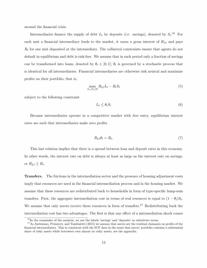
Intermediaries finance the supply of debt Lt by deposits (i.e. savings), denoted by St.16 For

each unit a financial intermediary lends to the market, it earns a gross interest of RLt and pays

Rt for one unit deposited at the intermediary. The collateral constraints ensure that agents do not

default in equilibrium and debt is risk-free. We assume that in each period only a fraction of savings

can be transformed into loans, denoted by θt ∈ [0, 1]; θt is governed by a stochastic process that

is identical for all intermediaries. Financial intermediaries are otherwise risk neutral and maximize

profits on their portfolio, that is,

maxLt,St≥0

RLtLt −RtSt (5)

subject to the following constraint

Lt ≤ θtSt (6)

Because intermediaries operate in a competitive market with free entry, equilibrium interest

rates are such that intermediaries make zero profits

RLtθt = Rt. (7)

This last relation implies that there is a spread between loan and deposit rates in this economy.

In other words, the interest rate on debt is always at least as large as the interest rate on savings,

or RLt ≥ Rt.

Transfers. The frictions in the intermediation sector and the presence of housing adjustment costs

imply that resources are used in the financial intermediation process and in the housing market. We

assume that these resources are redistributed back to households in form of type-specific lump-sum

transfers. First, the aggregate intermediation cost in terms of real resources is equal to (1− θt)St.

We assume that only savers receive these resources in form of transfers.17 Redistributing back the

intermediation cost has two advantages. The first is that any effect of a intermediation shock comes16In the remainder of the analysis, we use the labels ’savings’ and ’deposits’ as substitute terms.17As Justiniano, Primiceri, and Tambalotti (2015) we assume that savers are the residual claimants on profits of the

financial intermediaries. This is consistent with the SCF data in the sense that savers’ portfolio contains a substantialshare of risky assets while borrowers own almost no risky assets, see the appendix.

13

through general equilibrium effects, and is not generated by an aggregate loss of resources. The

second advantage is computational, as the re-distribution of resources makes sure that aggregate

consumption is a function of aggregate endowment only, an essential requirement for the application

of the concept of wealth recursive equilibria proposed by Kubler and Schmedders (2003) to our

framework.18

Second, realized housing adjustment costs are redistributed directly to the households who bear

them. This avoids externalities across household types due to the presence of housing adjustment

costs and makes sure that housing adjustment costs affect the housing demand for each household

type only at the margin.

To provide a formal summary of the discussion above, we set the per-capita household type

specific transfers equal to Υbt = Ψb(hbt) for borrowers and Υst = (1− θt)St/ns + Ψs(hst) for savers.

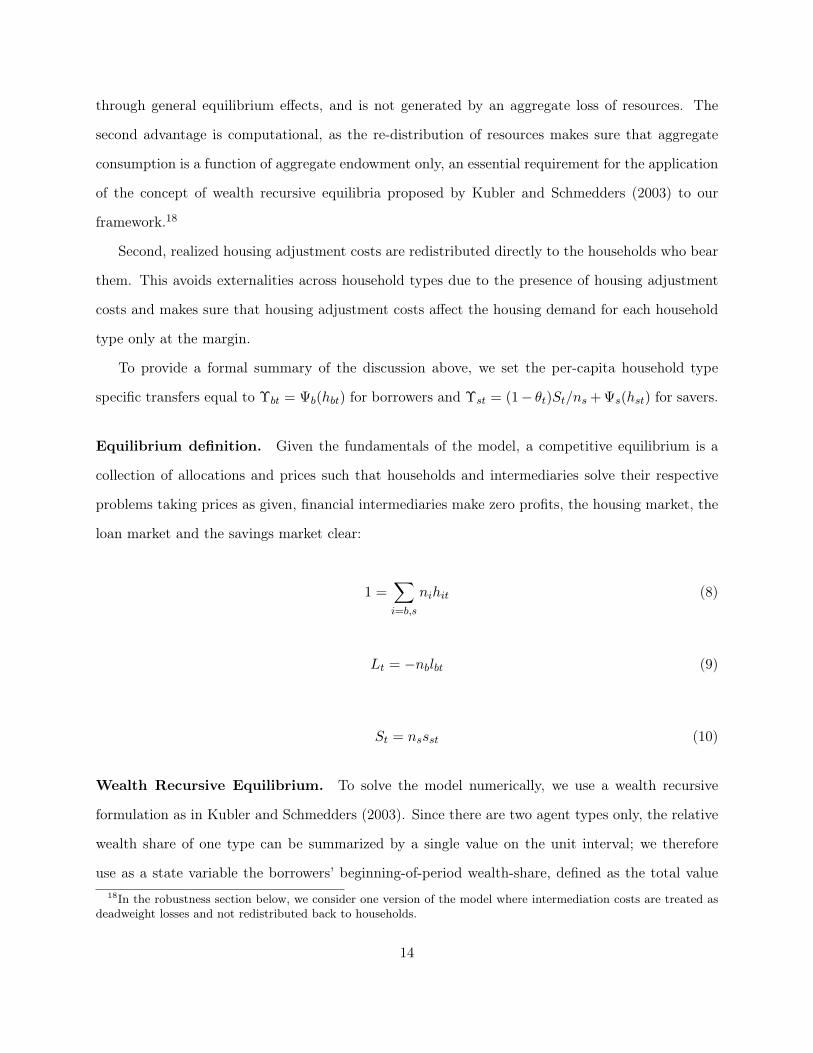
Equilibrium definition. Given the fundamentals of the model, a competitive equilibrium is a

collection of allocations and prices such that households and intermediaries solve their respective

problems taking prices as given, financial intermediaries make zero profits, the housing market, the

loan market and the savings market clear:

1 =∑i=b,s

nihit (8)

Lt = −nblbt (9)

St = nssst (10)

Wealth Recursive Equilibrium. To solve the model numerically, we use a wealth recursive

formulation as in Kubler and Schmedders (2003). Since there are two agent types only, the relative

wealth share of one type can be summarized by a single value on the unit interval; we therefore

use as a state variable the borrowers’ beginning-of-period wealth-share, defined as the total value18In the robustness section below, we consider one version of the model where intermediation costs are treated as

deadweight losses and not redistributed back to households.

14

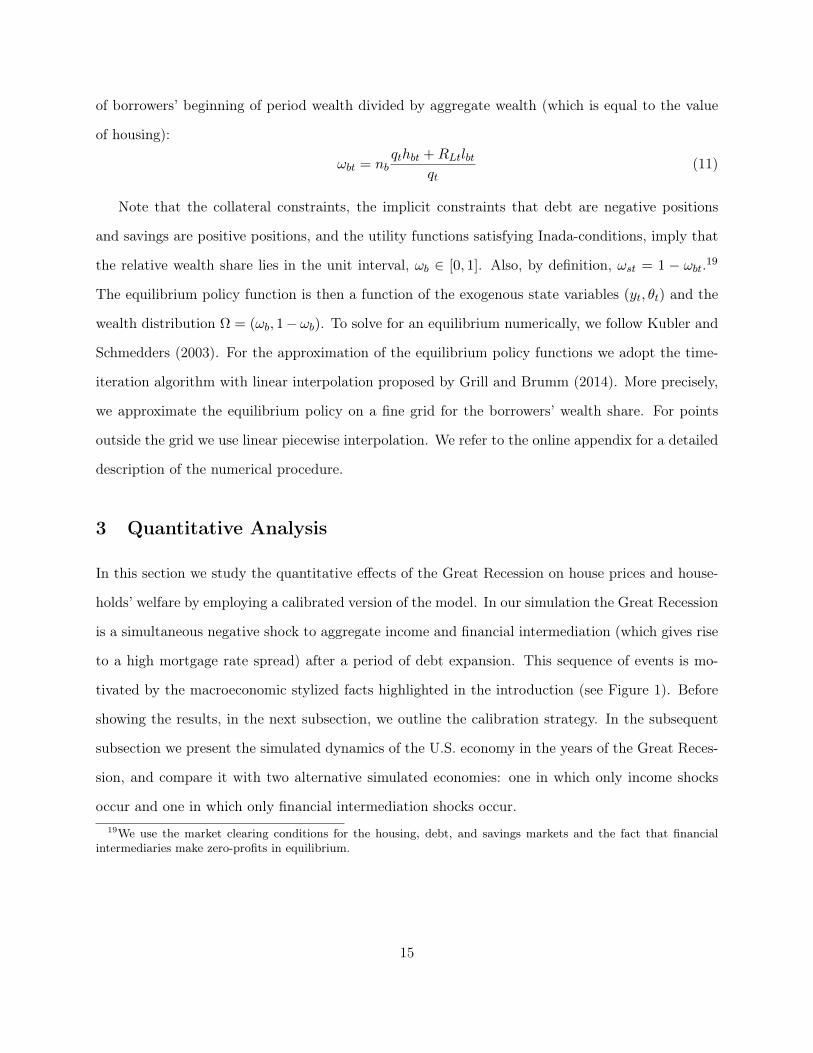
of borrowers’ beginning of period wealth divided by aggregate wealth (which is equal to the value

of housing):

ωbt = nbqthbt +RLtlbt

qt(11)

Note that the collateral constraints, the implicit constraints that debt are negative positions

and savings are positive positions, and the utility functions satisfying Inada-conditions, imply that

the relative wealth share lies in the unit interval, ωb ∈ [0, 1]. Also, by definition, ωst = 1 − ωbt.19

The equilibrium policy function is then a function of the exogenous state variables (yt, θt) and the

wealth distribution Ω = (ωb, 1−ωb). To solve for an equilibrium numerically, we follow Kubler and

Schmedders (2003). For the approximation of the equilibrium policy functions we adopt the time-

iteration algorithm with linear interpolation proposed by Grill and Brumm (2014). More precisely,

we approximate the equilibrium policy on a fine grid for the borrowers’ wealth share. For points

outside the grid we use linear piecewise interpolation. We refer to the online appendix for a detailed

description of the numerical procedure.

3 Quantitative Analysis

In this section we study the quantitative effects of the Great Recession on house prices and house-

holds’ welfare by employing a calibrated version of the model. In our simulation the Great Recession

is a simultaneous negative shock to aggregate income and financial intermediation (which gives rise

to a high mortgage rate spread) after a period of debt expansion. This sequence of events is mo-

tivated by the macroeconomic stylized facts highlighted in the introduction (see Figure 1). Before

showing the results, in the next subsection, we outline the calibration strategy. In the subsequent

subsection we present the simulated dynamics of the U.S. economy in the years of the Great Reces-

sion, and compare it with two alternative simulated economies: one in which only income shocks

occur and one in which only financial intermediation shocks occur.19We use the market clearing conditions for the housing, debt, and savings markets and the fact that financial

intermediaries make zero-profits in equilibrium.

15

3.1 Calibration

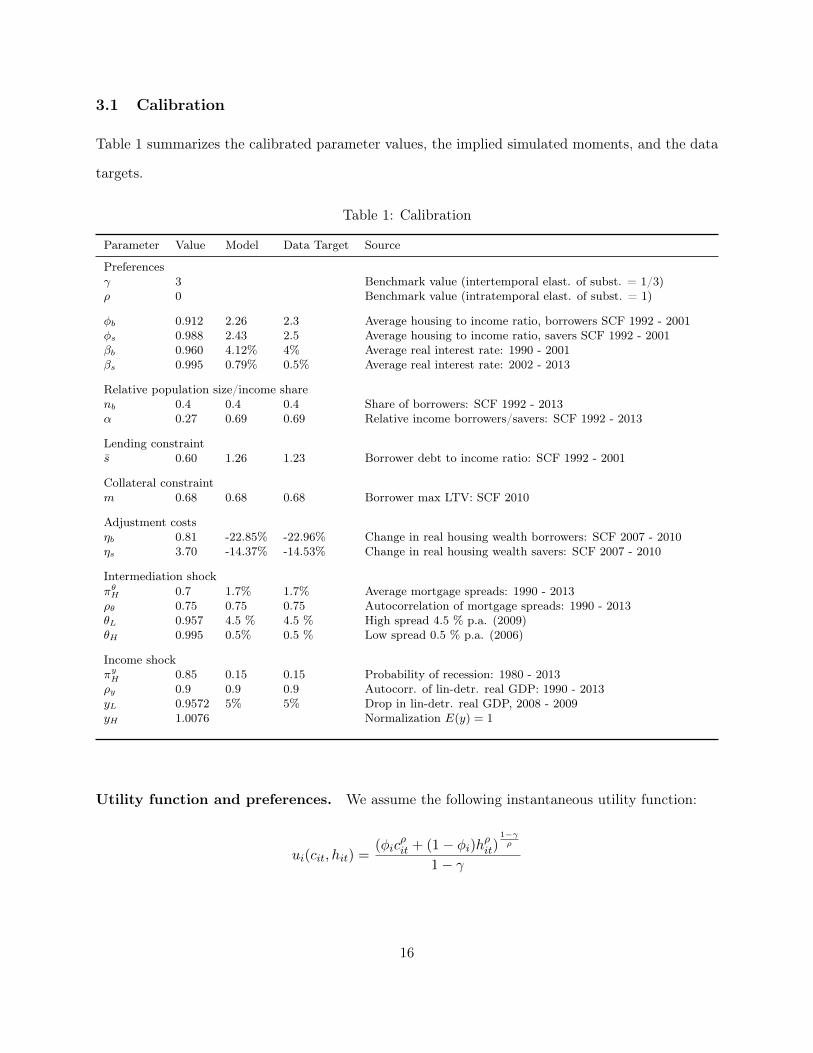
Table 1 summarizes the calibrated parameter values, the implied simulated moments, and the data

targets.

Table 1: Calibration

Parameter Value Model Data Target Source

Preferencesγ 3 Benchmark value (intertemporal elast. of subst. = 1/3)ρ 0 Benchmark value (intratemporal elast. of subst. = 1)

φb 0.912 2.26 2.3 Average housing to income ratio, borrowers SCF 1992 - 2001φs 0.988 2.43 2.5 Average housing to income ratio, savers SCF 1992 - 2001βb 0.960 4.12% 4% Average real interest rate: 1990 - 2001βs 0.995 0.79% 0.5% Average real interest rate: 2002 - 2013

Relative population size/income sharenb 0.4 0.4 0.4 Share of borrowers: SCF 1992 - 2013α 0.27 0.69 0.69 Relative income borrowers/savers: SCF 1992 - 2013

Lending constraints 0.60 1.26 1.23 Borrower debt to income ratio: SCF 1992 - 2001

Collateral constraintm 0.68 0.68 0.68 Borrower max LTV: SCF 2010

Adjustment costsηb 0.81 -22.85% -22.96% Change in real housing wealth borrowers: SCF 2007 - 2010ηs 3.70 -14.37% -14.53% Change in real housing wealth savers: SCF 2007 - 2010

Intermediation shockπθH 0.7 1.7% 1.7% Average mortgage spreads: 1990 - 2013ρθ 0.75 0.75 0.75 Autocorrelation of mortgage spreads: 1990 - 2013θL 0.957 4.5 % 4.5 % High spread 4.5 % p.a. (2009)θH 0.995 0.5% 0.5 % Low spread 0.5 % p.a. (2006)

Income shockπyH 0.85 0.15 0.15 Probability of recession: 1980 - 2013ρy 0.9 0.9 0.9 Autocorr. of lin-detr. real GDP: 1990 - 2013yL 0.9572 5% 5% Drop in lin-detr. real GDP, 2008 - 2009yH 1.0076 Normalization E(y) = 1

Utility function and preferences. We assume the following instantaneous utility function:

ui(cit, hit) =(φic

ρit + (1− φi)hρit)

1−γρ

1− γ

16

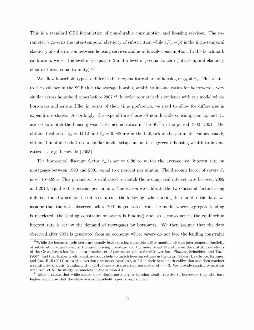
This is a standard CES formulation of non-durable consumption and housing services. The pa-

rameter γ governs the inter-temporal elasticity of substitution while 1/(1− ρ) is the intra-temporal

elasticity of substitution between housing services and non-durable consumption. In the benchmark

calibration, we set the level of γ equal to 3 and a level of ρ equal to zero (intratemporal elasticity

of substitution equal to unity).20

We allow household types to differ in their expenditure share of housing or φb 6= φs. This relates

to the evidence in the SCF that the average housing wealth to income ratios for borrowers is very

similar across household types before 2007.21 In order to match this evidence with our model where

borrowers and savers differ in terms of their time preference, we need to allow for differences in

expenditure shares. Accordingly, the expenditure shares of non-durable consumption, φb and φs,

are set to match the housing wealth to income ratios in the SCF in the period 1992- 2001. The

obtained values of φb = 0.912 and φs = 0.988 are in the ballpark of the parameter values usually

obtained in studies that use a similar model setup but match aggregate housing wealth to income

ratios, see e.g. Iacoviello (2005).

The borrowers’ discount factor βb is set to 0.96 to match the average real interest rate on

mortgages between 1990 and 2001, equal to 4 percent per annum. The discount factor of savers βs

is set to 0.995. This parameter is calibrated to match the average real interest rate between 2002

and 2013, equal to 0.5 percent per annum. The reason we calibrate the two discount factors using

different time frames for the interest rates is the following: when taking the model to the data, we

assume that the data observed before 2001 is generated from the model where aggregate lending

is restricted (the lending constraint on savers is binding) and, as a consequence, the equilibrium

interest rate is set by the demand of mortgages by borrowers. We then assume that the data

observed after 2001 is generated from an economy where savers do not face the lending constraint20While the business cycle literature usually features a log-separable utility function with an intertemporal elasticity

of substitution equal to unity, the asset pricing literature and the more recent literature on the distributive effectsof the Great Recession focus on a broader set of parameter values for risk aversion. Piazzesi, Schneider, and Tuzel(2007) find that higher levels of risk aversions help to match housing returns in the data. Glover, Heathcote, Krueger,and Ríos-Rull (2014) use a risk aversion parameter equal to γ = 2.5 in their benchmark calibration and then conducta sensitivity analysis. Similarly, Hur (2016) uses a risk aversion parameter of γ = 3. We provide sensitivity analysiswith respect to the utility parameters in the section 3.4.

21Table 4 shows that while savers show significantly higher housing wealth relative to borrowers they also havehigher income so that the share across household types is very similar.

17

anymore due to secular changes in the financial intermediation sector. Due to the additional funds

provided by savers, borrowers expand increase their demand for mortgages up to the borrowing

limit (given by the collateral constraint) and the equilibrium interest rate is determined by the

unconstrained supply of funds by savers.22

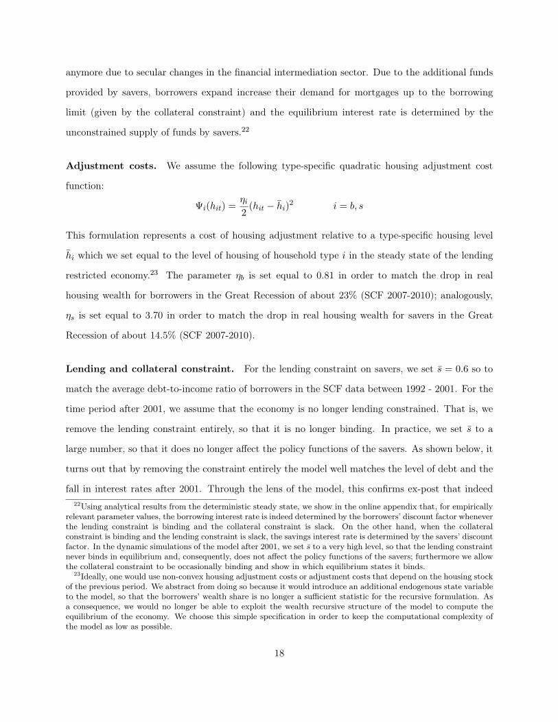
Adjustment costs. We assume the following type-specific quadratic housing adjustment cost

function:

Ψi(hit) =ηi2

(hit − hi)2 i = b, s

This formulation represents a cost of housing adjustment relative to a type-specific housing level

hi which we set equal to the level of housing of household type i in the steady state of the lending

restricted economy.23 The parameter ηb is set equal to 0.81 in order to match the drop in real

housing wealth for borrowers in the Great Recession of about 23% (SCF 2007-2010); analogously,

ηs is set equal to 3.70 in order to match the drop in real housing wealth for savers in the Great

Recession of about 14.5% (SCF 2007-2010).

Lending and collateral constraint. For the lending constraint on savers, we set s = 0.6 so to

match the average debt-to-income ratio of borrowers in the SCF data between 1992 - 2001. For the

time period after 2001, we assume that the economy is no longer lending constrained. That is, we

remove the lending constraint entirely, so that it is no longer binding. In practice, we set s to a

large number, so that it does no longer affect the policy functions of the savers. As shown below, it

turns out that by removing the constraint entirely the model well matches the level of debt and the

fall in interest rates after 2001. Through the lens of the model, this confirms ex-post that indeed22Using analytical results from the deterministic steady state, we show in the online appendix that, for empirically

relevant parameter values, the borrowing interest rate is indeed determined by the borrowers’ discount factor wheneverthe lending constraint is binding and the collateral constraint is slack. On the other hand, when the collateralconstraint is binding and the lending constraint is slack, the savings interest rate is determined by the savers’ discountfactor. In the dynamic simulations of the model after 2001, we set s to a very high level, so that the lending constraintnever binds in equilibrium and, consequently, does not affect the policy functions of the savers; furthermore we allowthe collateral constraint to be occasionally binding and show in which equilibrium states it binds.

23Ideally, one would use non-convex housing adjustment costs or adjustment costs that depend on the housing stockof the previous period. We abstract from doing so because it would introduce an additional endogenous state variableto the model, so that the borrowers’ wealth share is no longer a sufficient statistic for the recursive formulation. Asa consequence, we would no longer be able to exploit the wealth recursive structure of the model to compute theequilibrium of the economy. We choose this simple specification in order to keep the computational complexity ofthe model as low as possible.

18

the economy was no longer lending constrained after 2001.

The parameter in the collateral constraint, governing the maximum loan to value ratio m is

calibrated to match the observed LTV of 0.68 for borrowers in 2010 according to SCF data. The

implicit assumption here is that between 2007 and 2010 - when the average leverage ratio of bor-

rowers in the data was at its peak - the collateral constraint for borrowers was binding. This allows

to pin down m. The obtained value for the maximum LTV of m = 0.68 is slightly lower than the

loan to value ratio for the mortgages of new home buyers that has been documented to be around

80% (e.g. Lee, Mayer, and Tracy, 2012). However, within our setting, higher values of this param-

eter, for instance m = 0.8, would imply an equilibrium leverage ratio that is not compatible with

micro and macro evidence. The reasons are two: first, aggregate leverage in our model coincides

with the leverage position of only a portion of the total population of households, the borrowers;

second, we abstract from mortgages at different maturity; accordingly, we average among new and

older home owners who have already paid back part of their mortgage. Keeping these reasons into

consideration, both in macro and micro data leverage ratios are lower than 80%.

Relative population size and income share of borrowers. We define borrowers in the SCF

data as financially constrained households with a negative net financial asset position.24 Following

Kaplan and Violante (2014), we define financially constrained households as those with an amount

of liquid assets that is lower than two months income.25 We find that 40 percent of all home owners

are borrowers, while the remaining are savers. We therefore set nb = 0.4. We set the non-labor

income share equal to α = 0.29 so to match the fact that on average the total income of borrowers

in the SCF data is 62 percent relative to the average total income of savers.26

24Net financial asset position is calculated as the difference between safe financial assets held in the portfolio minustotal debt. Safe financial assets are defined as the sum of savings bonds, directly held bonds, the cash value of lifeinsurances, certificates of deposits, quasi-liquid retirement accounts and all other financial assets. Total debt is thesum of debt secured by primary residence, the debt secured by other residential property, credit card debt balance,debt lines on primary residences and all other forms of debt.

25Liquid assets are the sum of money market, checking, savings and call accounts, directly held mutual funds,stocks, bonds, and T-Bills, net of credit card debt

26In the model, the ratio of average incomes is given by nb(1−α)(1−α)ns+α

; given the value for nb this ratio is uniquelydetermined by α. Also notice that qualitatively the results on welfare do not depend on the value of α; it just helpsto improve the fit of the model to the data.

19

Exogenous shocks. The stochastic processes for the exogenous state variables yt and θt are

assumed to be statistically independent.27

We assume that both the aggregate income and the intermediation spread shock follow each

a two-state Markov process with realizations yt = yL, yH and θt = θL, θH, respectively. The

transition probabilities are given by:

πsij = (1− ρs)πsj + δijρs for i, j = H,L; s = θ, y

where δij = 1 if i = j and 0 otherwise; πsj > 0 is the unconditional probability of shock s being

in state j, and by definition we have∑

j πsj = 1. The parameter ρs governs the persistence of the

shock s = θ, y.28

For the financial intermediation shock, we set θL = 0.957, θH = 0.995, and ρθ = 0.75 so to

match the autocorrelation, the average spread, and a high spread of 4.5 percent, in line with the

data. Given these values, we set the unconditional probability of a high intermediation efficiency,

P (θ = θH), to 0.75, so to match the average spread in the data between 1990 - 2013 (equal to 1.7

percent per annum).

For the income shock, we choose yH and yL to match a normalized average of E(y) = 1 and an

average peak-to-trough drop in GDP of 5% during a recession. We set ρy = 0.9 so to match the

autocorrelation of yearly log real GDP after removing a linear trend between 1990 - 2013.

To summarize, the exogenous state space is given by Σ = (yH , θH), (yL, θH), (yH , θL), (yL, θL)

and - given the assumption that income and intermediation processes are uncorrelated - the tran-

sition matrix for the exogenous process is the Kronecker product of the individual transition prob-

ability matrices for the income shock and the intermediation shock, respectively.

Matching the moments. It is worth pointing out that there is not a one-to-one mapping between

the parameters in the utility and adjustment cost function and their targets. Hence we follow an27We conducted a VAR analysis for GDP growth and spreads for different lag-lengths and orderings and found

only weak evidence for significant spillover terms and no evidence for a contemporaneous correlation between GDPinnovations and innovations to mortgage spreads. Only in one specification, the null of Granger-causality of outputgrowth on spreads is rejected, for spreads the Null is never rejected.

28See Backus, Gregory, and Zin (1989) and Mendoza (1991).

20

iterative procedure to jointly find values for βb, βs, φb, φs, ηb, ηs, and s so to minimize the distance

between simulated and data moments. That is, given the relative population and income shares,

and given the calibration of the exogenous processes, we first guess values for the above parameters,

solve and simulate the model, and then compare the computed moments to their counterparts in the

data. If they do not match, we change the values and repeat until they do. Overall, this calibration

procedure leads to a quite satisfactorily match between model and data moments, as shown in Table

1. The numerical details (solution method, simulation, and calibration) are explained in detail in

the online appendix.

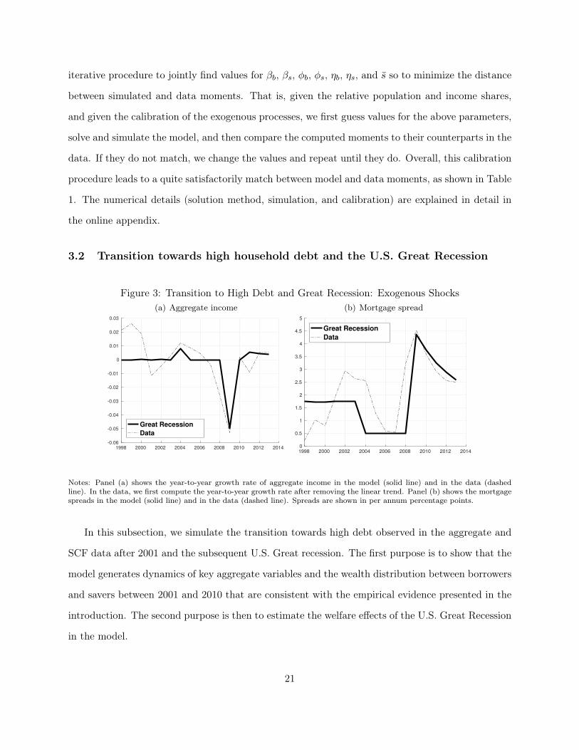
3.2 Transition towards high household debt and the U.S. Great Recession

Figure 3: Transition to High Debt and Great Recession: Exogenous Shocks(a) Aggregate income

1998 2000 2002 2004 2006 2008 2010 2012 2014

-0.06

-0.05

-0.04

-0.03

-0.02

-0.01

0

0.01

0.02

0.03

Great Recession

Data

(b) Mortgage spread

1998 2000 2002 2004 2006 2008 2010 2012 2014

0

0.5

1

1.5

2

2.5

3

3.5

4

4.5

5

Great Recession

Data

Notes: Panel (a) shows the year-to-year growth rate of aggregate income in the model (solid line) and in the data (dashedline). In the data, we first compute the year-to-year growth rate after removing the linear trend. Panel (b) shows the mortgagespreads in the model (solid line) and in the data (dashed line). Spreads are shown in per annum percentage points.

In this subsection, we simulate the transition towards high debt observed in the aggregate and

SCF data after 2001 and the subsequent U.S. Great recession. The first purpose is to show that the

model generates dynamics of key aggregate variables and the wealth distribution between borrowers

and savers between 2001 and 2010 that are consistent with the empirical evidence presented in the

introduction. The second purpose is then to estimate the welfare effects of the U.S. Great Recession

in the model.

21

In detail, we simulate the lending restricted economy (low s) for a long time series so that the

model converges to its ergodic wealth distribution. This corresponds to the situation previous to

2001 when mortgage debt-to-income is low. Then, we assume that in date 2004 (the first year

in the SCF data where borrowers debt-to-income ratio increased dramatically), households learn

unexpectedly that the limit on deposits s is removed so that the lending constraint is no longer

binding.29 This change in s represents the un-bounding of credit limits that lead to an increase

in supply of mortgages and, eventually, to an increase in household mortgage debt. Following this

change, savers are no longer savings-constrained, re-optimize and therefore the economy converges to

the new stationary equilibrium without lending constraints. Along this transition path, we feed into

the model the sequences of the exogenous income shocks and financial intermediation shocks that

are consistent with aggregate income and mortgage rate spreads in the data, as shown in Figure 3.

Panel (a) shows the evolution of aggregate income. As in the data, income slightly increases around

2004 and then drops by 5 percent in 2009 when the recession is at its peak. Similarly, as shown

in panel (b), we impose a series for the mortgage spread such that the mortgage spread falls to its

lowest level in the years preceding the recession and then jumps to 4.5 percent in 2009.30 Because

the exogenous processes are both two-state stationary Markov processes, we average over many

economies, so that for the periods before 2004 and after 2010 income and spreads have converged

already or return to their respective average values.

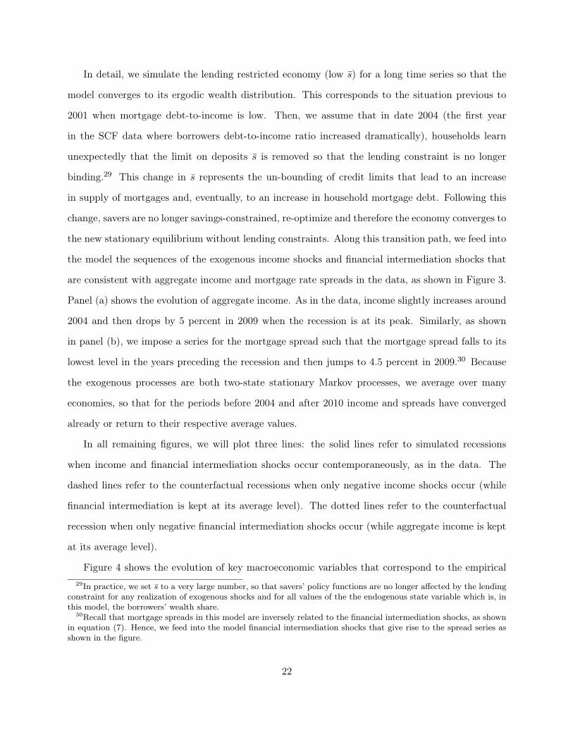
In all remaining figures, we will plot three lines: the solid lines refer to simulated recessions

when income and financial intermediation shocks occur contemporaneously, as in the data. The

dashed lines refer to the counterfactual recessions when only negative income shocks occur (while

financial intermediation is kept at its average level). The dotted lines refer to the counterfactual

recession when only negative financial intermediation shocks occur (while aggregate income is kept

at its average level).

Figure 4 shows the evolution of key macroeconomic variables that correspond to the empirical29In practice, we set s to a very large number, so that savers’ policy functions are no longer affected by the lending

constraint for any realization of exogenous shocks and for all values of the the endogenous state variable which is, inthis model, the borrowers’ wealth share.

30Recall that mortgage spreads in this model are inversely related to the financial intermediation shocks, as shownin equation (7). Hence, we feed into the model financial intermediation shocks that give rise to the spread series asshown in the figure.

22

Figure 4: Transition to High Debt and Great Recession in the Model: Debt, House Price, InterestRates

(a) debt-to-income ratio, borrowers

1998 2000 2002 2004 2006 2008 2010 2012 2014

1

1.2

1.4

1.6

1.8

2

Great Recession

Income shock

Fin. Int. shock

(b) House price

1998 2000 2002 2004 2006 2008 2010 2012 2014

0.8

0.9

1

1.1

1.2

1.3

1.4

1.5

1.6

Great Recession

Income shock

Fin. Int. shock

(c) Mortgage interest rate

1998 2000 2002 2004 2006 2008 2010 2012 2014

-3

-2

-1

0

1

2

3

4

5

6

Great Recession

Income shock

Fin. Int. shock

(d) Real interest rate

1998 2000 2002 2004 2006 2008 2010 2012 2014

-3

-2

-1

0

1

2

3

4

5

6

Great Recession

Income shock

Fin. Int. shock

series displayed in Figure 1. Panel (a) plots the behavior of borrowers’ debt-to-income ratio. The

model can account for the tremendous increase in borrowers’ debt-to-income ratio as observed in

the data between 2001 and 2007. In the model, this increase is mainly driven by the increase in

aggregate lending after the removal of the lending constraint. Low mortgage spreads in the years

2004-2007 only partially explain the increase in leverage in the years that precede the recession.

When the recession hits, the de-leveraging process is mainly explained by the negative financial

intermediation shock; in fact, in the income only counterfactual where the spread remains at its

average level, we observe that borrowers’ leverage drops very little.

Panel (b) shows the dynamics of the house price; the model can account for a large fraction

of both the increase and decrease in aggregate house prices, although some part of the boom-bust

23

cycle remains unexplained by the model. Our quantitative results suggest that the increase in house

prices is explained by the increase in credit supply after 2001, while the drop is largely explained

by the drop in aggregate income and, to some extent, by the high mortgage spreads.

Panels (c) and (d) show the dynamics of mortgage and real interest rates. In 2004, the increase

in aggregate lending generates a decrease in interest rates. In the recession, the real interest rate

drops, on impact, by about 4.26 percentage points, as a result of both income and financial inter-

mediation shocks. The economic mechanism is the following: in the recession, borrowers and savers

experience a negative income shock which induces a drop in their non-durable consumption and

leading to a drop in house prices. As a result the collateral constraint tightens. The financial inter-

mediation shock, on top of the income shock, drives a wedge between borrowing and lending interest

rate. Ceteris paribus, this leads borrowers to de-leverage and sell their housing, leading to further

deflationary pressure on house prices. This mechanism tightens the collateral constraint even more

and induces a further downward spiral in de-leveraging and in cutting consumption. Therefore, the

drop in housing and non-durable consumption is stronger for the borrowers. Savers, on the other

hand, cut on non-durable consumption while increasing housing, exploiting low aggregate prices as

we will discuss in more detail below. The drop in borrowing due to the tightening of the collateral

constraint generates a drop in the real interest rates. Because of the increase in the spreads, while

the real interest rate declines, the mortgage interest rate remains virtually constant on impact (-0.08

percentage points), in line with the dynamics we observe in the data between 2007 and 2009.

Figure 5 shows the dynamics of variables introduced in Figure 2 implied by the simulations of

the model. The solid lines in panels (a) and (b) show the simulated dynamics of housing wealth to

income ratio in the Great Recession for borrowers and savers, respectively, in the model defined as

q · hi/yi i = b, s. The solid line in panel (c) show the simulated dynamics of the borrowers’ wealth

share as defined in equation (11). The model replicates the increase in housing wealth over income

ratio for both borrowers and savers after 2001 and the larger decline for the borrowers in the Great

Recession. This translates into a decline of wealth share accruing to borrowers relative to savers in

the Great Recession comparable with the evidence from the SCF in Figure 2.

Figure 6 shows the implied model dynamics for consumption of borrowers and savers, respec-

24

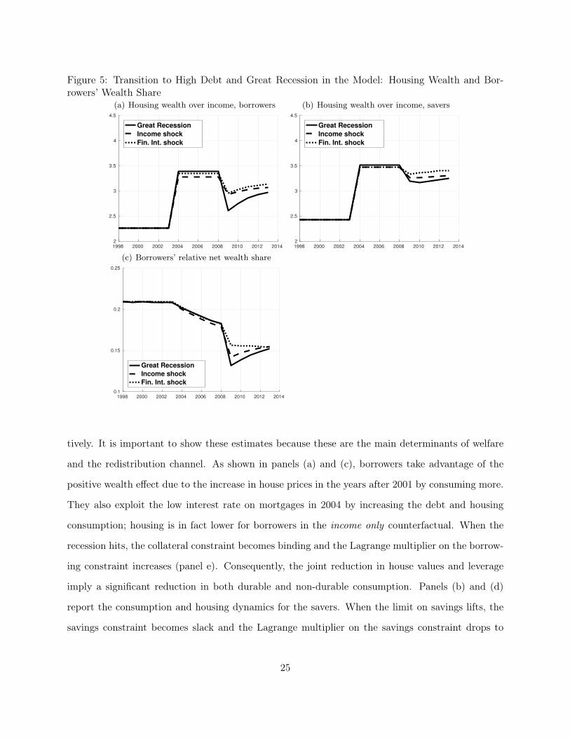
Figure 5: Transition to High Debt and Great Recession in the Model: Housing Wealth and Bor-rowers’ Wealth Share

(a) Housing wealth over income, borrowers

1998 2000 2002 2004 2006 2008 2010 2012 2014

2

2.5

3

3.5

4

4.5

Great Recession

Income shock

Fin. Int. shock

(b) Housing wealth over income, savers

1998 2000 2002 2004 2006 2008 2010 2012 2014

2

2.5

3

3.5

4

4.5

Great Recession

Income shock

Fin. Int. shock

(c) Borrowers’ relative net wealth share

1998 2000 2002 2004 2006 2008 2010 2012 2014

0.1

0.15

0.2

0.25

Great Recession

Income shock

Fin. Int. shock

tively. It is important to show these estimates because these are the main determinants of welfare

and the redistribution channel. As shown in panels (a) and (c), borrowers take advantage of the

positive wealth effect due to the increase in house prices in the years after 2001 by consuming more.

They also exploit the low interest rate on mortgages in 2004 by increasing the debt and housing

consumption; housing is in fact lower for borrowers in the income only counterfactual. When the

recession hits, the collateral constraint becomes binding and the Lagrange multiplier on the borrow-

ing constraint increases (panel e). Consequently, the joint reduction in house values and leverage

imply a significant reduction in both durable and non-durable consumption. Panels (b) and (d)

report the consumption and housing dynamics for the savers. When the limit on savings lifts, the

savings constraint becomes slack and the Lagrange multiplier on the savings constraint drops to

25

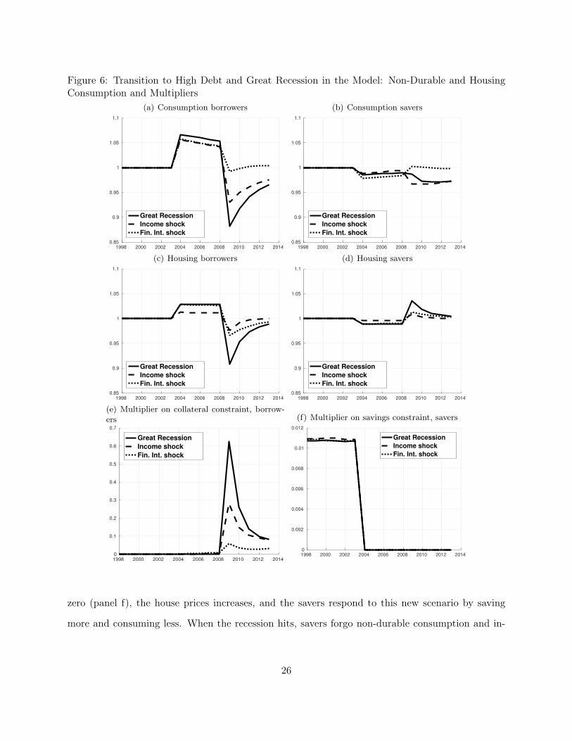
Figure 6: Transition to High Debt and Great Recession in the Model: Non-Durable and HousingConsumption and Multipliers

(a) Consumption borrowers

1998 2000 2002 2004 2006 2008 2010 2012 2014

0.85

0.9

0.95

1

1.05

1.1

Great Recession

Income shock

Fin. Int. shock

(b) Consumption savers

1998 2000 2002 2004 2006 2008 2010 2012 2014

0.85

0.9

0.95

1

1.05

1.1

Great Recession

Income shock

Fin. Int. shock

(c) Housing borrowers

1998 2000 2002 2004 2006 2008 2010 2012 2014

0.85

0.9

0.95

1

1.05

1.1

Great Recession

Income shock

Fin. Int. shock

(d) Housing savers

1998 2000 2002 2004 2006 2008 2010 2012 2014

0.85

0.9

0.95

1

1.05

1.1

Great Recession

Income shock

Fin. Int. shock

(e) Multiplier on collateral constraint, borrow-ers

1998 2000 2002 2004 2006 2008 2010 2012 2014

0

0.1

0.2

0.3

0.4

0.5

0.6

0.7

Great Recession

Income shock

Fin. Int. shock

(f) Multiplier on savings constraint, savers

1998 2000 2002 2004 2006 2008 2010 2012 2014

0

0.002

0.004

0.006

0.008

0.01

0.012

Great Recession

Income shock

Fin. Int. shock

zero (panel f), the house prices increases, and the savers respond to this new scenario by saving

more and consuming less. When the recession hits, savers forgo non-durable consumption and in-

26

crease their level of housing, exploiting the low level of house prices. This induces a redistribution

which persistently affects the welfare of the households. However, as shown in panel (b), the spread

and the income shocks imply different dynamics of non-durable consumption for the savers with

respect to the borrowers. While the spread shock implies a drop in consumption for the borrowers,

it instead, implies an increase for the savers. The de-leveraging process for the borrowers due to

the financial intermediation shock implies a wealth redistribution process which allows savers to

increase their net wealth and, finally, their non-durable consumption. In the next subsection we

report the welfare implications of these dynamics.

3.3 Welfare effects of the Great Recession

This section summarizes the welfare implications of the Great Recession for borrowers and savers.

We compute the welfare gains of the recession as the compensation - in percent of total consumption

(i.e. the aggregate of housing services and non-durable consumption) - needed each period for all

future periods to make agents indifferent between the expected life-time utility in 2007 (i.e. the

year just before the recession hits) and the expected life-time utility in 2009 (i.e. the year where

output growth is minus 5 percent and mortgage spread is at 4.5%). Formally, the total consumption

equivalent welfare gains for household type i = b, s are implicitly defined:

Vi(yL, θL, ω2009) = Vi(yH , θH , ω2007, λi)

where Vi(y, θ, ω) is the value function of household type i as a function of the exogenous processes

and the wealth distribution ω. Given the assumptions about the instantaneous utility function we

can write the welfare gain for household type i = b, s explicitly as

λi =

exp(1− βi)(Vi(yL, θL, ω2009)− Vi(yH , θH , ω2007)) − 1 γ = 1(Vi(yL,θL,ω2009)Vi(yH ,θH ,ω2007)

) 11−γ − 1 γ 6= 1

(12)

We refer to these estimates as ‘welfare gains’. Negative numbers therefore reflect the welfare

losses. The formula (12) clarifies where the transition dynamics matter for the estimated welfare

27

gains: through the dynamics of the wealth share of borrowers, ωt, as shown in panel (c) of Figure 5.

After the transition from the lending restricted to the unrestricted economy the wealth distribution

only converges slowly to the new ergodic wealth distribution. Therefore, the actual level of the

wealth share along the transition path affects the estimated welfare gains.

The main results on welfare are summarized in Table 2. The first six columns of the table show,

respectively, the percent change in housing wealth averaged over all households, labeled ∆q, the

percent change of housing wealth for borrowers and savers, labeled ∆(qhi) for i = b, s, and the

absolute percentage point change in the relative wealth share of borrowers, denoted by ∆ωb. The

relative wealth share is a direct measure of wealth distribution in the data and the model. The

trough-to-peak changes in the real interest rates on mortgages and savings are shown in columns

labeled ∆(RL) and ∆(R) between 2007 and 2009 (trough relative to pre-recession peak). In the last

two columns of the table we show the welfare gains of the recession in 2009 relative to the pre-crisis

peak in 2007, denoted by λb for borrowers and λs for savers. In the first row of the table we show

data moments. In the panel of the table labeled ’Benchmark model’ we report the welfare impact

of the Great Recession and compare these results to two counter-factual scenarios: when there is

only aggregate income shocks and when there is only a financial intermediation shock.

We find that the borrowers’ welfare loss in the Great Recession is significantly larger than that

of the savers. This result says that, when there is a drop in aggregate house prices, borrowers

are less able to cushion the wealth loss and de-leverage. Because of the de-leveraging, they reduce

consumption and the amount of housing which allows savers to buy housing when it is cheap; as a

result savers can buffer the negative welfare effects of the housing wealth drop.

We decompose the total effect into the effect that stems from the negative income and financial

intermediation shock, respectively, by feeding into the model one shock at the time while leaving

the other shock at its average level. The results for these counterfactuals are shown in the rows

labeled income shock and financial intermediation shock. We have the following results: i) about

70% of the drop in house prices in the Great Recession is due to the income shock, while the 30%

is caused by the financial intermediation shock; ii) the financial intermediation shock, although

causing an on-impact drop of housing wealth for borrowers and savers, implies an overall positive

28

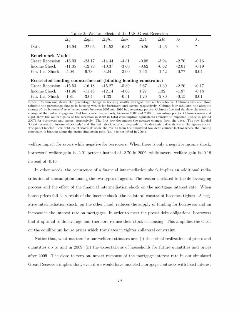
Table 2: Welfare effects of the U.S. Great Recession∆q ∆qhb ∆qhs ∆ωb ∆RL ∆R λb λs

Data -16.94 -22.96 -14.53 -6.37 -0.26 -4.26 ? ?

Benchmark ModelGreat Recession -16.93 -23.17 -14.44 -4.81 -0.08 -3.94 -2.70 -0.16Income Shock -11.05 -12.79 -10.37 -3.60 -0.62 -0.62 -2.01 -0.19Fin. Int. Shock -5.08 -9.73 -3.24 -3.00 2.46 -1.52 -0.77 0.04

Restricted lending counterfactual (binding lending constraint)Great Recession -15.53 -16.18 -15.27 -5.39 2.67 -1.39 -2.20 -0.17Income Shock -11.96 -11.48 -12.14 -4.06 1.27 1.32 -1.97 -0.18Fin. Int. Shock -1.81 -3.04 -1.33 -0.51 1.20 -2.80 -0.15 0.01

Notes: Column one shows the percentage change in housing wealth averaged over all households. Columns two and threetabulate the percentage change in housing wealth for borrowers and savers, respectively. Column four tabulates the absolutechange of the borrowers’ relative net worth between 2007 and 2010 in percentage points. Columns five and six show the absolutechange of the real mortgage and Fed funds rate, respectively, between 2007 and 2009 in percentage points. Columns seven andeight show the welfare gains of the recession in 2009 in total consumption equivalents (relative to expected utility in period2007) for borrowers and savers, respectively. The first row documents the average changes from the data. The row labeled’Great recession’, ’income shock only’ and ’fin. int. shock only’ corresponds to the dynamic paths shown in the figures above.The panel labeled ’Low debt counterfactual’ show the results from the simulated low debt counter-factual where the lendingconstraint is binding along the entire simulation path (i.e. s is not lifted in 2004).

welfare impact for savers while negative for borrowers. When there is only a negative income shock,

borrowers’ welfare gain is -2.01 percent instead of -2.70 in 2009, while savers’ welfare gain is -0.19

instead of -0.16.

In other words, the occurrence of a financial intermediation shock implies an additional redis-

tribution of consumption among the two types of agents. The reason is related to the de-leveraging

process and the effect of the financial intermediation shock on the mortgage interest rate. When

house prices fall as a result of the income shock, the collateral constraint becomes tighter. A neg-

ative intermediation shock, on the other hand, reduces the supply of funding for borrowers and an

increase in the interest rate on mortgages. In order to meet the preset debt obligations, borrowers

find it optimal to de-leverage and therefore reduce their stock of housing. This amplifies the effect

on the equilibrium house prices which translates in tighter collateral constraint.

Notice that, what matters for our welfare estimates are: (i) the actual realizations of prices and

quantities up to and in 2009; (ii) the expectations of households for future quantities and prices

after 2009. The close to zero on-impact response of the mortgage interest rate in our simulated

Great Recession implies that, even if we would have modeled mortgage contracts with fixed interest

29

rates (the most common mortgage contract in the USA as shown in Calza, Monacelli, and Stracca,

2013), the welfare gain caused by the actual realizations of the prices and quantities would have

been unaffected by this assumption. However, since both exogenous shock processes are persistent

but mean reverting, households assume that all variables will eventually return to their stationary

levels after the Great Recession. To the extent that fixed interest rates on outstanding mortgages

affect the households’ expectations about the future levels of prices and quantities, they could have

impacted our welfare estimates. The direction of the bias naturally depends on the expectations

about the wealth share and the sensitivity of equilibrium borrowing and house prices to the financial

intermediation shock under this assumption.

As a second counterfactual exercise, we replicate the simulation of the Great Recession in the

lending constrained economy, that is, s is kept at the value of 0.60 so that it is binding in equi-

librium. We want to study to which extent the Great Recession would have impacted households’

welfare if we would have not observed the large increase in aggregate household mortgage debt in

the years that preceded the recession. The results are shown in the second panel of the Table 2

labeled Restricted lending counterfactual. When aggregate credit (and therefore mortgage debt) is

restricted to be low, the welfare impact of the Great Recession is significantly smaller for borrow-

ers while bigger for savers. This difference is mainly related to the different quantitative impact

of financial intermediation shocks when aggregate leverage is lower. The redistribution related to

the de-leveraging process is, in fact, significantly smaller when the level of mortgage supply and

households’ indebtedness in the economy is lower. This finding provides quantitative support for

the hypothesis of Mian and Sufi (2015) that the combination of high debt with a collapse in housing

values represents one of the main cause of the larger welfare losses for leveraged households in the

U.S. Great Recession.

Overall, our results lead to the conclusion that, while both types of agents experienced a welfare

loss in the Great Recession, savers were able to cushion themselves from the negative impact of

the negative aggregate shocks. This conclusion, while qualitatively comparable with the findings in

Hur (2016), highlights a different mechanism that comes from a negative financial intermediation

shock coupled with high level of outstanding households’ leverage. Regarding the size of the welfare

30

losses of the Great Recession, our estimates are in the same order of magnitude of large recessions

as found by Krueger, Mitman, and Perri (2016).

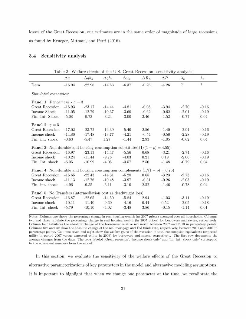
3.4 Sensitivity analysis

Table 3: Welfare effects of the U.S. Great Recession: sensitivity analysis∆q ∆qhb ∆qhs ∆ωb ∆RL ∆R λb λs

Data -16.94 -22.96 -14.53 -6.37 -0.26 -4.26 ? ?

Simulated economies:

Panel 1: Benchmark - γ = 3Great Recession -16.93 -23.17 -14.44 -4.81 -0.08 -3.94 -2.70 -0.16Income Shock -11.05 -12.79 -10.37 -3.60 -0.62 -0.62 -2.01 -0.19Fin. Int. Shock -5.08 -9.73 -3.24 -3.00 2.46 -1.52 -0.77 0.04

Panel 2: γ = 5Great Recession -17.02 -23.72 -14.39 -5.40 2.56 -1.40 -2.94 -0.16Income shock -14.80 -17.48 -13.77 -4.21 -0.54 -0.56 -2.28 -0.19Fin. int. shock -0.63 -5.47 1.27 -1.44 2.93 -1.05 -0.62 0.04

Panel 3: Non-durable and housing consumption substitutes (1/(1− ρ) = 4.55)Great Recession -16.97 -23.13 -14.47 -5.56 0.68 -3.21 -2.74 -0.16Income shock -10.24 -11.44 -9.76 -4.03 0.21 0.19 -2.06 -0.19Fin. Int. shock -6.05 -10.99 -4.05 -3.57 2.50 -1.48 -0.79 0.04

Panel 4: Non-durable and housing consumption complements (1/(1− ρ) = 0.75)Great Recession -16.65 -22.43 -14.31 -5.28 0.65 -3.23 -2.73 -0.16Income shock -11.13 -12.76 -10.48 -3.97 -0.31 -0.26 -2.03 -0.19Fin. int. shock -4.96 -9.55 -3.11 -3.10 2.52 -1.46 -0.78 0.04

Panel 5: No Transfers (intermediation cost as deadweight loss)Great Recession -16.87 -22.65 -14.50 -5.84 2.94 -1.03 -3.11 -0.19Income shock -10.11 -11.40 -9.60 -4.16 0.44 0.52 -2.05 -0.18Fin. Int. shock -5.79 -10.10 -4.02 -3.48 3.86 -0.15 -1.14 0.01

Notes: Column one shows the percentage change in real housing wealth (at 2007 prices) averaged over all households. Columnstwo and three tabulate the percentage change in real housing wealth (in 2007 prices) for borrowers and savers, respectively.Column four tabulates the absolute change of the borrowers’ relative net worth between 2007 and 2010 in percentage points.Columns five and six show the absolute change of the real mortgage and Fed funds rate, respectively, between 2007 and 2009 inpercentage points. Columns seven and eight show the welfare gains of the recession in total consumption equivalents (expectedutility in period 2007 versus expected utility in 2009) for borrowers and savers, respectively. The first row documents theaverage changes from the data. The rows labeled ’Great recession’, ’income shock only’ and ’fin. int. shock only’ correspondto the equivalent numbers from the model.

In this section, we evaluate the sensitivity of the welfare effects of the Great Recession to

alternative parameterizations of key parameters in the model and alternative modeling assumptions.

It is important to highlight that when we change one parameter at the time, we recalibrate the

31

adjustment cost parameters as well, so that the alternative economy matches, as close as possible,

the drop in housing wealth in the Great Recession for both household types. The results are

summarized in in Table 3. For convenience, the table also repeats the benchmark results in the top

panel. Notice that, the direct comparison of all simulated economies confirms that the benchmark

version outperform the other versions in matching the data targets.

Intertemporal elasticity of substitution. In our benchmark calibration we set γ = 3, so that

the intertemporal elasticity of substitution (IES), given by 1/γ, is one third. Panel 2 of Table 3

reports the welfare estimates for γ = 5, i.e. a lower IES than in the benchmark equal to 1/5.31

With respect to the benchmark calibration, the new parametrization of γ = 5 leads to a higher

housing adjustment cost for borrowers (from 0.81 in the benchmark to 1.65) and lower adjustment

costs for savers (from 3.7 in the benchmark to 1.7) in order to match the observed drop in housing

wealth for the two types of households in the Great Recession. With this calibration (Panel 2 of

Table 3), we find that income shocks explain a larger share of the house price drop than the financial

intermediation shock, in contrast to the benchmark. With lower IES, in a recession, housing demand

drops more for both household types as a result of the income shock, and house prices have to fall

more so that households still want to consume the housing. This is a standard mechanism in

the consumption based asset price model, see Piazzesi, Schneider, and Tuzel (2007) and Glover,

Heathcote, Krueger, and Ríos-Rull (2014). However, when a financial intermediation shock hits,

the higher housing adjustment costs on borrowers increases their cost of selling the house, while

the opposite is true for the savers. This means there is less supply and higher demand for housing

after the financial intermediation shock, relative to the benchmark model, which translate into

less movement in prices. The relatively smaller effect of financial intermediation shock on house

prices implies the collateral constraint to be relatively less tight and therefore a smaller interaction

effect in the Great Recession when both shocks hit together; as a result, the saving interest rate

goes down by less in the Great Recession with respect to the benchmark, implying a on-impact31We also conducted robustness for lower values of γ = 1. However, for values of γ lower than 3 the model generates

a drop in aggregate housing wealth in the recession that is too low when compared to the data. Hence, given ourcalibration strategy, the algorithm could not find adjustment cost parameters to match the observed drop in housingwealth.

32

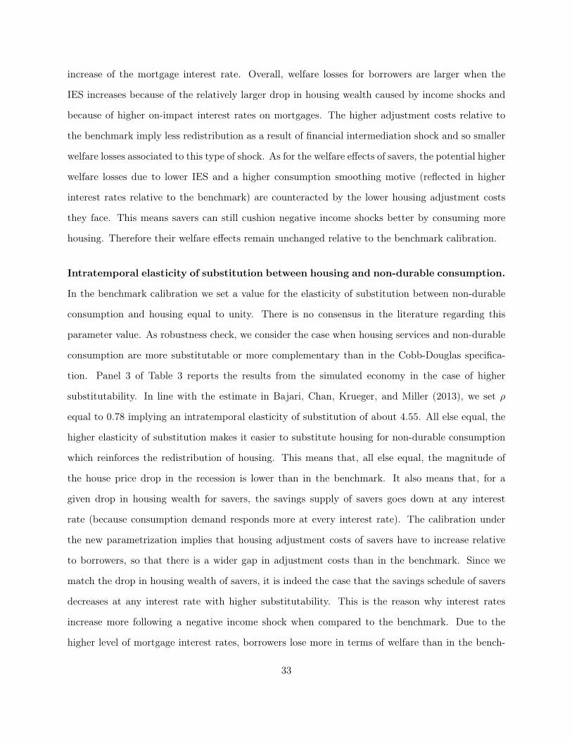
increase of the mortgage interest rate. Overall, welfare losses for borrowers are larger when the

IES increases because of the relatively larger drop in housing wealth caused by income shocks and

because of higher on-impact interest rates on mortgages. The higher adjustment costs relative to

the benchmark imply less redistribution as a result of financial intermediation shock and so smaller

welfare losses associated to this type of shock. As for the welfare effects of savers, the potential higher

welfare losses due to lower IES and a higher consumption smoothing motive (reflected in higher

interest rates relative to the benchmark) are counteracted by the lower housing adjustment costs

they face. This means savers can still cushion negative income shocks better by consuming more

housing. Therefore their welfare effects remain unchanged relative to the benchmark calibration.

Intratemporal elasticity of substitution between housing and non-durable consumption.

In the benchmark calibration we set a value for the elasticity of substitution between non-durable

consumption and housing equal to unity. There is no consensus in the literature regarding this

parameter value. As robustness check, we consider the case when housing services and non-durable

consumption are more substitutable or more complementary than in the Cobb-Douglas specifica-

tion. Panel 3 of Table 3 reports the results from the simulated economy in the case of higher

substitutability. In line with the estimate in Bajari, Chan, Krueger, and Miller (2013), we set ρ

equal to 0.78 implying an intratemporal elasticity of substitution of about 4.55. All else equal, the

higher elasticity of substitution makes it easier to substitute housing for non-durable consumption

which reinforces the redistribution of housing. This means that, all else equal, the magnitude of

the house price drop in the recession is lower than in the benchmark. It also means that, for a

given drop in housing wealth for savers, the savings supply of savers goes down at any interest

rate (because consumption demand responds more at every interest rate). The calibration under

the new parametrization implies that housing adjustment costs of savers have to increase relative

to borrowers, so that there is a wider gap in adjustment costs than in the benchmark. Since we

match the drop in housing wealth of savers, it is indeed the case that the savings schedule of savers

decreases at any interest rate with higher substitutability. This is the reason why interest rates

increase more following a negative income shock when compared to the benchmark. Due to the

higher level of mortgage interest rates, borrowers lose more in terms of welfare than in the bench-

33

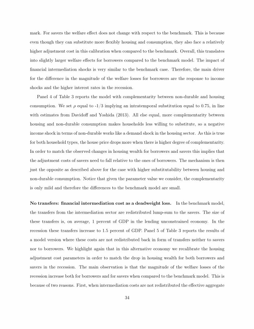
mark. For savers the welfare effect does not change with respect to the benchmark. This is because

even though they can substitute more flexibly housing and consumption, they also face a relatively

higher adjustment cost in this calibration when compared to the benchmark. Overall, this translates

into slightly larger welfare effects for borrowers compared to the benchmark model. The impact of

financial intermediation shocks is very similar to the benchmark case. Therefore, the main driver

for the difference in the magnitude of the welfare losses for borrowers are the response to income

shocks and the higher interest rates in the recession.

Panel 4 of Table 3 reports the model with complementarity between non-durable and housing

consumption. We set ρ equal to -1/3 implying an intratemporal substitution equal to 0.75, in line

with estimates from Davidoff and Yoshida (2013). All else equal, more complementarity between

housing and non-durable consumption makes households less willing to substitute, so a negative

income shock in terms of non-durable works like a demand shock in the housing sector. As this is true

for both household types, the house price drops more when there is higher degree of complementarity.

In order to match the observed changes in housing wealth for borrowers and savers this implies that

the adjustment costs of savers need to fall relative to the ones of borrowers. The mechanism is then

just the opposite as described above for the case with higher substitutability between housing and

non-durable consumption. Notice that given the parameter value we consider, the complementarity

is only mild and therefore the differences to the benchmark model are small.

No transfers: financial intermediation cost as a deadweight loss. In the benchmark model,

the transfers from the intermediation sector are redistributed lump-sum to the savers. The size of

these transfers is, on average, 1 percent of GDP in the lending unconstrained economy. In the

recession these transfers increase to 1.5 percent of GDP. Panel 5 of Table 3 reports the results of

a model version where these costs are not redistributed back in form of transfers neither to savers

nor to borrowers. We highlight again that in this alternative economy we recalibrate the housing

adjustment cost parameters in order to match the drop in housing wealth for both borrowers and

savers in the recession. The main observation is that the magnitude of the welfare losses of the

recession increase both for borrowers and for savers when compared to the benchmark model. This is

because of two reasons. First, when intermediation costs are not redistributed the effective aggregate

34

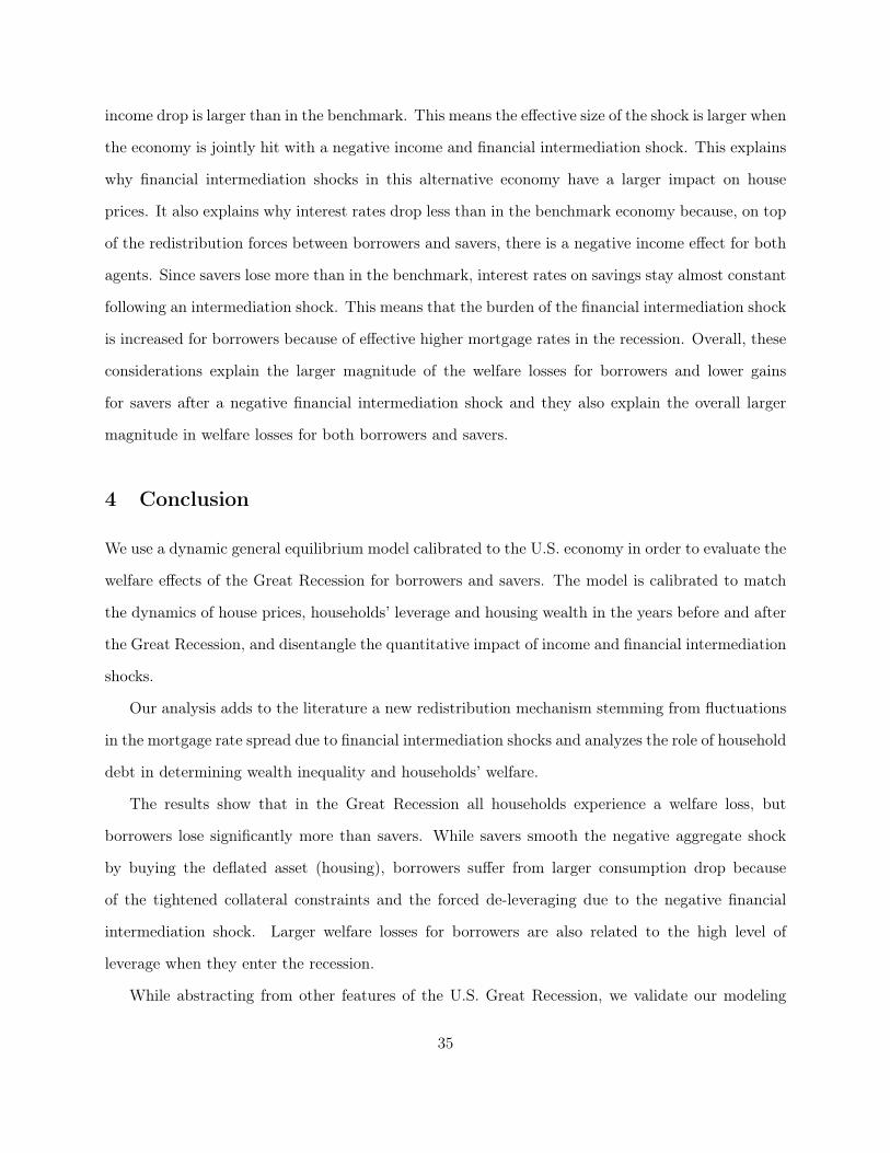
income drop is larger than in the benchmark. This means the effective size of the shock is larger when

the economy is jointly hit with a negative income and financial intermediation shock. This explains

why financial intermediation shocks in this alternative economy have a larger impact on house

prices. It also explains why interest rates drop less than in the benchmark economy because, on top

of the redistribution forces between borrowers and savers, there is a negative income effect for both

agents. Since savers lose more than in the benchmark, interest rates on savings stay almost constant

following an intermediation shock. This means that the burden of the financial intermediation shock

is increased for borrowers because of effective higher mortgage rates in the recession. Overall, these

considerations explain the larger magnitude of the welfare losses for borrowers and lower gains

for savers after a negative financial intermediation shock and they also explain the overall larger

magnitude in welfare losses for both borrowers and savers.

4 Conclusion

We use a dynamic general equilibrium model calibrated to the U.S. economy in order to evaluate the

welfare effects of the Great Recession for borrowers and savers. The model is calibrated to match

the dynamics of house prices, households’ leverage and housing wealth in the years before and after

the Great Recession, and disentangle the quantitative impact of income and financial intermediation

shocks.

Our analysis adds to the literature a new redistribution mechanism stemming from fluctuations

in the mortgage rate spread due to financial intermediation shocks and analyzes the role of household

debt in determining wealth inequality and households’ welfare.

The results show that in the Great Recession all households experience a welfare loss, but

borrowers lose significantly more than savers. While savers smooth the negative aggregate shock

by buying the deflated asset (housing), borrowers suffer from larger consumption drop because

of the tightened collateral constraints and the forced de-leveraging due to the negative financial

intermediation shock. Larger welfare losses for borrowers are also related to the high level of

leverage when they enter the recession.

While abstracting from other features of the U.S. Great Recession, we validate our modeling

35

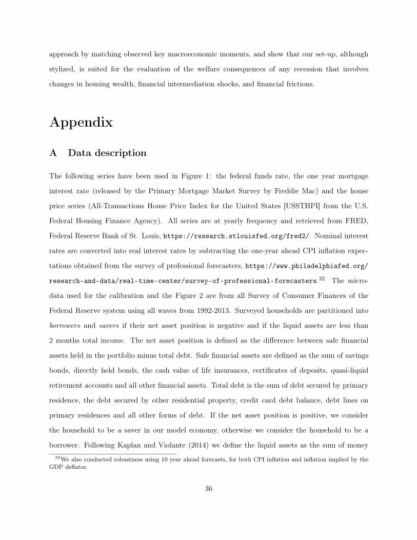
approach by matching observed key macroeconomic moments, and show that our set-up, although

stylized, is suited for the evaluation of the welfare consequences of any recession that involves

changes in housing wealth, financial intermediation shocks, and financial frictions.

Appendix

A Data description

The following series have been used in Figure 1: the federal funds rate, the one year mortgage

interest rate (released by the Primary Mortgage Market Survey by Freddie Mac) and the house

price series (All-Transactions House Price Index for the United States [USSTHPI] from the U.S.

Federal Housing Finance Agency). All series are at yearly frequency and retrieved from FRED,

Federal Reserve Bank of St. Louis, https://research.stlouisfed.org/fred2/. Nominal interest

rates are converted into real interest rates by subtracting the one-year ahead CPI inflation expec-

tations obtained from the survey of professional forecasters, https://www.philadelphiafed.org/

research-and-data/real-time-center/survey-of-professional-forecasters.32 The micro-

data used for the calibration and the Figure 2 are from all Survey of Consumer Finances of the

Federal Reserve system using all waves from 1992-2013. Surveyed households are partitioned into

borrowers and savers if their net asset position is negative and if the liquid assets are less than

2 months total income. The net asset position is defined as the difference between safe financial

assets held in the portfolio minus total debt. Safe financial assets are defined as the sum of savings

bonds, directly held bonds, the cash value of life insurances, certificates of deposits, quasi-liquid

retirement accounts and all other financial assets. Total debt is the sum of debt secured by primary

residence, the debt secured by other residential property, credit card debt balance, debt lines on

primary residences and all other forms of debt. If the net asset position is positive, we consider

the household to be a saver in our model economy, otherwise we consider the household to be a

borrower. Following Kaplan and Violante (2014) we define the liquid assets as the sum of money32We also conducted robustness using 10 year ahead forecasts, for both CPI inflation and inflation implied by the

GDP deflator.

36

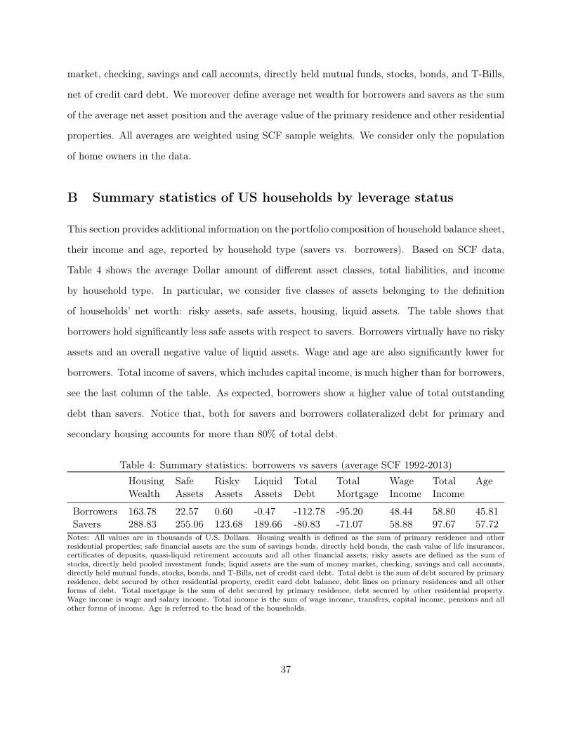
market, checking, savings and call accounts, directly held mutual funds, stocks, bonds, and T-Bills,

net of credit card debt. We moreover define average net wealth for borrowers and savers as the sum

of the average net asset position and the average value of the primary residence and other residential

properties. All averages are weighted using SCF sample weights. We consider only the population

of home owners in the data.

B Summary statistics of US households by leverage status

This section provides additional information on the portfolio composition of household balance sheet,

their income and age, reported by household type (savers vs. borrowers). Based on SCF data,

Table 4 shows the average Dollar amount of different asset classes, total liabilities, and income

by household type. In particular, we consider five classes of assets belonging to the definition

of households’ net worth: risky assets, safe assets, housing, liquid assets. The table shows that

borrowers hold significantly less safe assets with respect to savers. Borrowers virtually have no risky

assets and an overall negative value of liquid assets. Wage and age are also significantly lower for

borrowers. Total income of savers, which includes capital income, is much higher than for borrowers,

see the last column of the table. As expected, borrowers show a higher value of total outstanding

debt than savers. Notice that, both for savers and borrowers collateralized debt for primary and

secondary housing accounts for more than 80% of total debt.

Table 4: Summary statistics: borrowers vs savers (average SCF 1992-2013)Housing Safe Risky Liquid Total Total Wage Total AgeWealth Assets Assets Assets Debt Mortgage Income Income

Borrowers 163.78 22.57 0.60 -0.47 -112.78 -95.20 48.44 58.80 45.81Savers 288.83 255.06 123.68 189.66 -80.83 -71.07 58.88 97.67 57.72

Notes: All values are in thousands of U.S. Dollars. Housing wealth is defined as the sum of primary residence and otherresidential properties; safe financial assets are the sum of savings bonds, directly held bonds, the cash value of life insurances,certificates of deposits, quasi-liquid retirement accounts and all other financial assets; risky assets are defined as the sum ofstocks, directly held pooled investment funds; liquid assets are the sum of money market, checking, savings and call accounts,directly held mutual funds, stocks, bonds, and T-Bills, net of credit card debt. Total debt is the sum of debt secured by primaryresidence, debt secured by other residential property, credit card debt balance, debt lines on primary residences and all otherforms of debt. Total mortgage is the sum of debt secured by primary residence, debt secured by other residential property.Wage income is wage and salary income. Total income is the sum of wage income, transfers, capital income, pensions and allother forms of income. Age is referred to the head of the households.

37

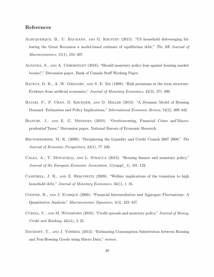
References

Albuquerque, B., U. Baumann, and G. Krustev (2015): “US household deleveraging fol-

lowing the Great Recession–a model-based estimate of equilibrium debt,” The BE Journal of

Macroeconomics, 15(1), 255–307.

Alpanda, S., and A. Ueberfeldt (2016): “Should monetary policy lean against housing market

booms?,” Discussion paper, Bank of Canada Staff Working Paper.

Backus, D. K., A. W. Gregory, and S. E. Zin (1989): “Risk premiums in the term structure:

Evidence from artificial economies,” Journal of Monetary Economics, 24(3), 371–399.

Bajari, P., P. Chan, D. Krueger, and D. Miller (2013): “A Dynamic Model of Housing

Demand: Estimation and Policy Implications,” International Economic Review, 54(2), 409–442.

Bianchi, J., and E. G. Mendoza (2010): “Overborrowing, Financial Crises and’Macro-

prudential’Taxes,” Discussion paper, National Bureau of Economic Research.

Brunnermeier, M. K. (2009): “Deciphering the Liquidity and Credit Crunch 2007–2008,” The

Journal of Economic Perspectives, 23(1), 77–100.

Calza, A., T. Monacelli, and L. Stracca (2013): “Housing finance and monetary policy,”

Journal of the European Economic Association, 11(suppl_1), 101–122.

Campbell, J. R., and Z. Hercowitz (2009): “Welfare implications of the transition to high

household debt,” Journal of Monetary Economics, 56(1), 1–16.

Cooper, R., and J. Ejarque (2000): “Financial Intermediation and Aggregate Fluctuations: A

Quantitative Analysis,” Macroeconomic Dynamics, 4(4), 423–447.

Cúrdia, V., and M. Woodford (2010): “Credit spreads and monetary policy,” Journal of Money,

Credit and Banking, 42(s1), 3–35.

Davidoff, T., and J. Yoshida (2013): “Estimating Consumption Substitution between Housing

and Non-Housing Goods using Macro Data,” mimeo.

38

Dell’Ariccia, G., D. Igan, and L. U. Laeven (2012): “Credit booms and lending standards:

Evidence from the subprime mortgage market,” Journal of Money, Credit and Banking, 44(2-3),

367–384.

Gilchrist, S., and E. Zakrajšek (2012): “Credit Spreads and Business Cycle Fluctuations,”

American Economic Review, 102(4), 1692–1720.

Glover, A., J. Heathcote, D. Krueger, and J.-V. Ríos-Rull (2014): “Intergenerational

Redistribution in the Great Recession,” Mimeo.

Grill, M., and J. Brumm (2014): “Computing Equilibria in Dynamic Models with Occasionally

Binding Constraints,” Journal of Economic Dynamics and Control, 38, 142–160.

Guerrieri, V., and G. Lorenzoni (2011): “Credit Crises, Precautionary Savings, and the Liq-

uidity Trap,” NBER Working Papers 17583, National Bureau of Economic Research, Inc.

Hall, R. E. (2011): “The High Sensitivity of Economic Activity to Financial Frictions,” The

Economic Journal, 121, 351–378.

Huo, Z., and J.-V. Ríos-Rull (2014): “Financial Frictions, Asset Prices, and the Great Reces-

sion,” Mimeo.

Hur, S. (2016): “The lost generation of the Great Recession,” Mimeo.

Iacoviello, M. (2005): “House Prices, Borrowing Constraints, and Monetary Policy in the Busi-

ness Cycle,” American Economic Review, 95(3), 739–764.

(2011): “Housing wealth and consumption,” International Encyclopedia of Housing and

Home, Elsevier.

Justiniano, A., G. E. Primiceri, and A. Tambalotti (2014): “The effects of the saving and

banking glut on the US economy,” Journal of International Economics, 92, S52–S67.

(2015): “Credit supply and the housing boom,” Discussion paper, National Bureau of

Economic Research.

39

Kalemli-Ozcan, S., E. Papaioannou, and F. Perri (2012): “Global banks and crisis transmis-

sion,” Journal of International Economics, 87(5), 495–510.

Kaplan, G., and G. L. Violante (2014): “A model of the consumption response to fiscal stimulus

payments,” Econometrica, 82(4), 1199–1239.

Kiyotaki, N., and J. Moore (1997): “Credit Cycles,” Journal of Political Economy, 105(2),

211–248.

Krueger, D., K. Mitman, and F. Perri (2016): “On the distribution of the welfare losses of

large recessions,” Discussion paper, National Bureau of Economic Research.

Kubler, F., and K. Schmedders (2003): “Stationary Equilibria in Asset-Pricing Models with

Incomplete Markets and Collateral,” Econometrica, 71(6), 1767–1793.

Kumhof, M., R. Rancière, and P. Winant (2015): “Inequality, leverage, and crises,” The

American Economic Review, 105(3), 1217–1245.

Landvoigt, T., M. Piazzesi, and M. Schneider (2015): “The housing market (s) of San Diego,”

American Economic Review, 105(4), 1371–1407.

Lee, D., C. J. Mayer, and J. Tracy (2012): “A new look at second liens,” Discussion paper,

National Bureau of Economic Research.

Mendoza, E. G. (1991): “Real Business Cycles in a Small Open Economy,” American Economic

Review, 81(4), 797–818.

Mian, A., and A. Sufi (2009): “The Consequences of Mortgage Credit Expansion: Evidence frome

the U.S. Mortgage Default Crisis,” Quarterly Journal of Economics, pp. 1499–1496.

(2010): “The Great Recession: Lessons from Microeconomic Data,” American Economic

Review: Papers and Proceedings, 100, 51–56.

(2015): House of Debt: How They (and You) Caused the Great Recession, and How We

Can Prevent It from Happening Again. University of Chicago Press.

40

Piazzesi, M., M. Schneider, and S. Tuzel (2007): “Housing, consumption and asset pricing,”

Journal of Financial Economics, 83(3), 531 – 569.

Quadrini, V., and J. J. Urban (2012): “Macroeconomic Effects of Financial Shocks,” American

Economic Review, 102(1), 238–71.

Smets, F., and R. Wouters (2007): “Shocks and frictions in US business cycles: A Bayesian

DSGE approach,” The American Economic Review, 97(3), 586–606.

41