Find and Replace: R&D Investment Following the Erosion of Existing Products Joshua L. Krieger Xuelin Li Richard T. Thakor

Working Paper 19-058

Working Paper 19-058

Copyright © 2020 by Joshua L. Krieger, Xuelin Li, and Richard T. Thakor.

Working papers are in draft form. This working paper is distributed for purposes of comment and discussion only. It may not be reproduced without permission of the copyright holder. Copies of working papers are available from the author.

Funding for this research was provided in part by Harvard Business School.

Find and Replace: R&D Investment Following the Erosion of Existing Products

Joshua L. Krieger Harvard Business School

Xuelin Li University of Minnesota

Richard T. Thakor University of Minnesota

Find and Replace: R&D Investment Following

the Erosion of Existing Products*

Joshua L. Krieger,† Xuelin Li,‡ and Richard T. Thakor§

April 21, 2021

Abstract

How do innovative firms react when existing products experience negative shocks? Weexplore this question with detailed project-level data from drug development firms. Us-ing FDA Public Health Advisories as idiosyncratic negative shocks to approved drugs, weexamine how drug makers react through investment decisions. Following these shocks,affected firms increase R&D expenditures, driven by a higher likelihood of acquiring ex-ternal innovations, rather than developing novel projects internally. Such acquisitionactivities are concentrated in firms with weak research pipelines. We also find that com-peting developers move resources away from the affected therapeutic areas. Our resultsshow how investments in specialized commercialization capital create path dependenciesand alter the direction of R&D investments.

Keywords: R&D Investments, Drug Development, Product Shocks, M&A, Biopharma-ceutical Industry, FDA

*For helpful comments and discussions, we thank Hengjie Ai, Ashish Arora (the editor), Pierre Azoulay,Frederico Belo, Daniel Carpenter, Lauren Cohen, Nuri Ersahin (discussant), Joshua Feng, Murray Frank,Craig Garthwaite (discussant), Sabrina Howell, Manuel Hermosilla, Pinar Karaca-Mandic, Anne MarieKnott (discussant), Danielle Li, Song Ma, Jeff Macher (discussant), Mahka Moeen (discussant), RamanaNanda, Dimitris Papanikolaou, Merih Sevilir (discussant), Myles Shaver, Andrei Shleifer, Ariel Stern, An-jan Thakor, Raj Vasu (discussant), Tracy Wang, Andy Winton, Yu Xu, Xintong Zhan (discussant), an AEand three anonymous referees, and seminar participants at University of Minnesota, Nanyang Techno-logical University, National University of Singapore, City University of Hong Kong, University of HongKong, and MIT Sloan, University of Utah Eccles School of Business, and participants at the MinnesotaCorporate Finance Conference, 2019 American Economic Association Meetings, Utah-BYU Winter StrategyConference, Duke-UNC Entrepreneurship Research Conference, Northwestern Kellogg Annual HealthcareMarkets Conference, 2019 Financial Intermediation Research Society Conference, 12th Annual Northwest-ern/USPTO Conference on Innovation Economics, 2019 ASHEcon Conference, and 2019 CICF Conference.Any remaining errors are ours alone.

†Harvard Business School, jkrieger@hbs.edu‡University of South Carolina, Moore School of Business, xuelin.li@moore.sc.edu§University of Minnesota, Carlson School of Management, and MIT LFE, rthakor@umn.edu

1 IntroductionCreative destruction relies on a diverse pipeline of new research and development

(R&D) opportunities, as well as a robust market for technologies. However, firms do not

make their R&D investment decisions in a vacuum. Anecdotally, the performance of ex-

isting products shapes upstream investment activities—both within and across firms.1

Yet, to understand how downstream performance influences upstream R&D requires a

systematic analysis of how firms reshuffle their project porfolio following shocks to ex-

isting products. As research pipelines are the primary fuel for an R&D-driven firm’s

survival, portfolio allocations across markets and sources of innovation (e.g., internal vs.

external) are crucial managerial decisions. Studying how downstream shocks shake up

these R&D priorities sheds light on how product outcomes (more generally) shape the

direction of innovative activity and demand in markets for technology.

This paper uses detailed project-level data to investigate how negative shocks to ex-

isting products impact firms’ R&D investments. To motivate our hypotheses, we first de-

velop a stylized theoretical model of staged firm R&D investment. Different from other

innovator “dilemmas,” we focus on “commercialization capital” investment and realloca-

tion decisions, and how they influence R&D pipeline decisions under the specter of neg-

ative product-market shocks.2 Commercialization capital includes investments in man-

ufacturing and distribution centers in the supply chain, advertising and relationships

with industry leaders (i.e., physicians) for marketing, and scientists for post-marketing

research.

In our model, a firm engages in staged R&D and may be affected by a negative profit

1For recent examples, see the media narratives around pharma mega mergers such as theBristol-Myers Squibb acquisition of biotechnology firm Celgene for $74 billion, and AbbVie’s pur-chase of Allergan for $63 billion, both on the heels of struggling R&D pipelines. https:

//www.wsj.com/articles/bristol-myers-squibb-to-acquire-celgene-11546517754; https://www.

wsj.com/articles/plan-on-more-pharma-megamergers-11562421600.2Examples of prior theories that highlight the incumbent disadvantages in innovating include Arrow’s

replacement effect (?), Christensen’s theory of disruptive innovation (?), uneven technology spillovers (?),and trapped factors (?).

1

shock to one of its products. The firm endogenously chooses the scale of its research port-

folio and its investment into commercialization capital, accounting for the possibility of a

negative shock. The specialization of this commercialization capital creates path depen-

dencies and alters the direction of R&D investments as firms seek to efficiently redeploy

commercialization capital. These dynamics generate the following main theoretical pre-

dictions. First, after experiencing a negative shock to existing products, affected firms

will increase R&D expenditures through acquisitions. Second, the acquisition activities

are concentrated among the affected firms with weaker research pipelines. Lastly, com-

peting firms do not make such acquisitions.

We provide empirical results consistent with these predictions. Specifically, we esti-

mate firms’ investment responses to the US Food and Drug Administration’s (FDA) Pub-

lic Health Advisories (PHAs) for approved drugs. We use detailed project-level data from

competitive intelligence databases to track PHA disclosures for approved drugs, as well

as internal and external R&D project investments and progress.3 The PHAs are based on

new adverse information about a company’s commercialized drug, such as previously-

unknown negative side effects. PHAs are plausibly exogenous and idiosyncratic events

for a specific drug—allowing us to identify the effects of a shock to existing products that

are distinct from other firm-specific or industry-wide developments.4 Our analysis con-

firms that PHAs lead to a reduction in the focal firm’s revenue, even when the event does

not involve a full product recall.

We employ a differences-in-differences approach to measuring the PHA response, us-

3The drug development industry provides an ideal context for studying the link between downstreamproduct shocks and upstream R&D investment choice because the regulatory structure and patent sys-tem allow the researcher to observe the full landscape of project investments. Other attractive features ofthis setting include the existence of an active “market for ideas” (??), and how firms often manage R&Dportfolios across multiple markets (diseases), technologies (drug targets), and development stages.

4Importantly, these shocks are specific to a particular drug and do not reveal new information aboutregulatory standards. Previous studies have generally used industry-level shocks to explore the effect ofthe product market on innovation outcomes. The potential shortcoming of such an approach is that suchshocks make it difficult to analyze competitor behavior. For example, recent papers by ? and ? find oppositeeffects in terms of the relationship between competitive shocks and innovation. Since the shocks we employare product-specific, they allow us to overcome the potential shortcomings of industry-level shocks. Section3.1 describes PHAs in more detail.

2

ing a three-year window around the PHA events and a control group of public drug com-

panies without PHAs. Our results imply that firms whose products experience a PHA

respond with a statistically significant 21% increase in R&D spending as a percentage of

total assets, relative to firms who do not experience PHA events in the same window. We

show these investments are primarily comprised of “external” R&D (acquisitions) rather

than “internal” R&D (new initiations). While the unconditional probability of acquisi-

tion is 11%, it increases dramatically to 39% in the post-PHA treatment window. After

controlling for firm characteristics and time trends, the main empirical results show a

significant 8 percentage point increase in the probability of external drug acquisitions

following PHA events, relative to control firms. In line with the replacement motive, the

new acquisition targets are in the same therapeutic areas as the PHA drug. By contrast,

we find no significant effect of PHAs on the propensity to initiate new internal projects.

These results are consistent with the story that wounded incumbents, with their ex-

isting base of “commercialization capital” in place (e.g., clinical trial operations, sales

teams, etc.), have a strategic incentive to continue operating in the areas in which they

hold a comparative advantage (e.g., ???). Rather than replenish their pipeline through

their own exploratory and early-stage R&D, they acquire drugs already in trials for the

very same diseases, for which they had already built up specialized assets.5

To establish the channels behind our model and results, we examine heterogeneity

across types of firms. Consistent with our model, we find that the focal firm acquisition

effects are stronger when the PHA involves drugs with relatively higher sales, and when

the affected firm has a weaker internal pipeline. Furthermore, our theory suggests that

firms will attempt to reallocate commercialization capital within the same therapeutic

areas, and we provide evidence of this reallocation using physician marketing payments

as an example of specialized downstream investments.

Next, we address alternative explanations for the post-PHA acquisition patterns using

5This is in line with empirical evidence that has shown an increase in innovative activity and abnormalreturns following acquisitions (e.g., ??).

3

competitor responses and a battery of robustness checks. We first show that competing

firms, which are contemporaneously developing drugs but have no approved products in

the PHA warned area, adjust their project investments along different lines.6 Rather than

increasing expenditures aimed at replacing the beleaguered PHA drug, these research

competitors re-shuffle their R&D portfolios away from the PHA area. In particular, they

are less likely to initiate new internal projects or trials, and are more likely to shut down

projects in the affected PHA area. These competitor spillovers help rule out the story that

PHA events trigger a race to fill the new product-market gap.

To test the robustness of our results, we conduct a number of additional analyses.

These tests include the re-specifying the window surrounding the PHA events, propensity-

score matching between treated and control firms, falsification/placebo tests that vary the

timing of PHA events, regressions including private firms, and accounting for timing of

the PHA relative to loss of marketing exclusivity. Our results survive these tests.

This paper is related to the internal capital markets literature on how shocks influence

investment across business lines (?????). R&D investment choices are not only horizon-

tal (across business lines), but also vertical (upstream in early-stage research and down-

stream in sales and marketing) and path-dependent.7 Our project level data allow us to

examine not only how a firm responds to the shock, but how that response depends on

organizational subdivisions within the firm. In contrast to much of the internal capital

markets literature, we find that rather than cutting expenditures after a negative shock,

pharmaceutical firms increase R&D spending in the affected therapeutic areas, and use

acquisitions to produce a replacement quickly.

Our paper also contributes to the literature on financing of innovation,8 and the de-

6In supplemental analyses, we also explore the affected firm’s product market competitors.7See ??? for examples of how a firm’s absorptive capacity, its ability to assimilate external knowledge,

changes the return to different types of R&D investments.8This literature evaluates how market conditions affect firm R&D investment and innovative output (??),

the productivity and direction of R&D efforts (????), and choice of financing instruments (???). Our paperis related to recent work on how a firm’s productivity in internal innovation affects decisions to invest inexternal ventures (??).

4

terminants of mergers and acquisitions.9 ? is particularly relevant, as they document that

greater “desperation” in a firm’s R&D pipeline is positively associated with engaging in

mergers and acquisitions. Along similar lines, ? show that firms in the pharmaceutical

and biotechnology industries tend to do mergers in response to deteriorating R&D condi-

tions. Like those prior papers, we also examine the R&D portfolio strength of innovative

firms. By evaluating the investment responses to unanticipated shocks, and comparing

how the response differs by portfolio strength, we supply micro-foundations and causal

evidence behind the desperation channel of acquisition and investment behavior.

We add to these various literatures in three distinct ways. First, our detailed portfo-

lio data allow us to track pipeline investments at the project level, and characterize their

source (in-house vs. in-licensed) and disease applications.10 Second, as plausibly exoge-

nous shocks to firms, PHAs help us overcome endogenous firm “quality” concerns (i.e.,

bad firms are bad at R&D so they turn to R&D acquisition). The idiosyncratic nature of

these PHAs also allows us to isolate the effect of shocks that are distinct from broader

changes in the market or economic conditions.11 Third, we account for the spillover ef-

fects by measuring how relevant competitors adjust their R&D investments in the wake

of PHAs.12

9This literature posits various explanations for engaging in acquisitions (e.g., ???). While these papersfocus on the acquisitions of whole firms, our data allow us to examine acquisitions of projects, and provideevidence of specific channels that motivate them.

10A set of recent papers use similar data to address related questions in drug development. ? use detailedpipeline data to measure how a positive financial shock (the introduction of Medicare Part D) impactsinvestments in molecular novelty; ? evaluates licensing choices and outcomes in the wake of clinical trialfailures; and ? study “killer acquisitions,” the practice of acquiring drug candidates in order to terminatepotential rivals. In contrast, this paper’s primary investment distinction is between internal and externalR&D expenditures in the wake of a negative, product-specific shock to approved drugs.

11Similar to prior work on product recalls (???), we use PHAs as shocks to both product areas and firmrevenues. ? and ? also use a related empirical strategy—black box warnings for prescription drugs, whichare a common follow-on to a PHA—to study regulatory events and their impact on demand and marketingactivity. ? uses a different type of FDA action, drug rejections, to study subsequent product abandonmentdecisions.

12Outside of the drug industry, these types of knowledge and market spillover have been measured atthe firm level, using patents (??). Project-specific spillover outcomes have proven more elusive in othersettings.

5

2 Conceptual FrameworkIn this section, we provide a description of our theoretical model and the main hy-

potheses it generates. We include the formal development of the model in the Online

Appendix.

Consider a firm that engages in staged R&D across three time periods. In the first

period, the firm makes an endogenous choice of the number of products to develop. It

incurs a fixed research infrastructure cost that is independent of product portfolio size

and also a per-product R&D cost. R&D then proceeds in the first period and the outcome

of is uncertain. At the end of the first period only some of the products survive.

Having observed how many products survived, the firm makes a second endogenous

choice—this time of how much to invest in commercialization capital to develop down-

stream assets for each of the surviving products. These downstream assets can be inter-

preted as investments for facilitating the commercialization of new products. This may

consist of knowledge stock and investments made in the sales, marketing, supply chain,

and clinical research teams that specialize in the area.13 The assumption is that such

assets are specialized at the product-market level, but are not effective outside of that

market. For example, while the infrastructure built to support a blockbuster cholesterol

drug might not be easily transferred to oncology markets, that capital should maintain

most of its value when being repurposed for another heart disease drug. We assume

that the firm’s investment payoff is a concavely increasing function of its investment in

commercialization capital.

The outcome of commercialization is also uncertain. At the end of the second period,

the firm observes how many products survived this phase. Then one of the surviving

13More specifically, late-stage and post-marketing clinical trials need experienced scientists and physi-cians to design trials, recruit certain patient groups and run large-scale studies. Drugs with different ex-pected volumes, modalities and formulation techniques (e.g., small molecules vs. biologics) might requiredifferent manufacturing capacity and know-how. Sales & marketing teams develop therapeutic area ex-pertise and form relationships with specialist doctors, who are seen as critical to the dissemination andadoption of new drugs.

6

products receives a PHA shock, which reduces its payoff to zero. The PHA shock also

creates slack commercialization capital that is vacated from the affected product, which

the firm can then reallocate to its existing products or to a new product it can acquire.

Given this, the firm then makes a third endogenous choice at the start of the third period

about whether to replace the product lost due to the PHA shock by acquiring a similar

product from another firm, or to simply proceed with one less product. If it chooses to

acquire a product from another firm, the price is endogenously solved for as well. We

assume that the firm has sufficient internal funds to make the acquisition.

Thus, the base model has four endogenous variables: (i) the initial product portfolio

size; (ii) the investment in and reallocation of commercialization capital; (iii) the decision

to replace a PHA-shocked product with a product acquired from another firm; and (iv)

and the price paid in the acquisition.

We then extend the base model in a number of ways. First, we relax our assumption

that the firm has sufficient internal funds available to acquire a product, and examine

the effect of financial frictions induced by adverse selection. Second, we discuss how an

affected firm would also choose to not internally initiate a new project in response to a

PHA, and furthermore how competitor firms would not engage in the same behavior as

affected firms. Finally, we describe how our results could also be micro-founded through

incomplete contracting.

The model generates a number of results in the form of testable hypotheses, which we

examine in our empirical results. First, after experiencing a negative shock to existing

products, our model predicts that affected firms will increase R&D expenditures through

acquisitions. The intuition is that, given its prior investment into commercialization cap-

ital, it is optimal for the firm to re-deploy the slack commercialization capital from the

PHA-afflicted product onto an externally-acquired project in the same therapeutic area

rather than under-utilizing that capital in its remaining project portfolio. This decision

is further made optimal due to gains from trade between the buying and selling firms.

7

Second, the acquisition decisions are concentrated among the affected firms with weaker

research pipelines. The intuition is that weaker firms have a relatively stronger incentive

to deploy their excess commercialization capital to serve a newly acquired project as op-

posed to their existing project lines. These illiquid downstream assets become the com-

parative advantage for the firm in markets for technology. When firms need to fund their

acquisitions using external financing, then it is only the weaker firms that find it optimal

to bear the cost of doing so that stems from financial frictions.14 Third, competing firms

not directly affected by the PHA will choose to abandon their research in the same area,

either by selling to the affected firm or potentially moving to other areas. Together, these

predictions provide a microfoundation for why firms may ramp up investments and pur-

sue “desperation” mergers and acquisitions after losing an existing revenue stream (?).

2.1 Managerial Implications

Our model carries the following managerial implications for R&D investments deci-

sions under the specter of product market shocks:

1. When faced with the possibility of future product market shocks, decisions about the level

of investment in commercialization capital should take into account how likely a firm’s

products are to be faced with such a shock. Frictions in reallocation of commercial-

ization capital lead to path-dependencies in R&D portfolios. If the firm targets

markets with non-trivial rates of negative product shocks (regulatory or otherwise),

then options for reallocating downstream assets in the event of a shock should play

prominently in valuing the initial product development opportunity. That is, man-

agers should recognize the gains from product market focus.

2. It may be optimal to replace negatively affected products via acquisitions of (same-market)

products from other firms. Thus, investments in commercialization capital connect

with a firm’s optimal source of R&D. This incentive will also vary across firms. Firms

14The assumption that such R&D-intensive firms need to rely on external financing to fund their opera-tions, given the large costs they face, is well-documented in the empirical literature. See ? for a review.

8

that have greater slack commercialization capital generated by a product shock—

such as a product with a high level of sales—will generate a stronger incentive to do

an acquisition.

3. Firms with weaker product portfolios should plan more on acquisitions The poorer the

firm’s R&D portfolio, the greater should be the firm’s interest in replacing the shocked

product. There are potential gains from trade—in other words, other firms operat-

ing in the same area may find it optimal to sell their products to a firm affected

by a negative product shock. Thus, firms with poorer product portfolios should

be more prepared—i.e. have unused debt capacity, excess cash, or other sources of

funding—to undertake such acquisitions.

4. R&D competitors may benefit indirectly from the reshuffling of products and pipelines.

Firms with related pipeline projects enjoy two upstream benefits of competitors’

negative product shocks: 1) the potential acquisition value of their projects may

go up significantly if the affected firm becomes a motivated buyer for a replace-

ment product, and 2) the shock may contain critical information about underlying

scientific, health and regulatory risks. That information can allow competitors to

reorganize their existing R&D investments efficiently (before sinking too much into

less flexible commercialization capital), or update their beliefs about how risky a

product area may be prior to R&D entry decisions.

Our model therefore provides implications both for how managers should respond

to negative product shocks, and also optimal investment decisions if such shocks are a

possibility. These responses will also depend on the realization of the firm’s R&D, and

the frictions the firm faces in the market.

9

3 Empirical Approach and Data

3.1 FDA Public Health Advisories

All drugs marketed to consumers in the United States are required to have completed

the Food and Drug Administration (FDA) drug approval process, which typically entails

three phases of human clinical trials and a final application review prior to approval.

Upon approval of a drug, the developing firm must update the drug’s prescription in-

formation for risk warnings and guidance discovered in the approval process. However,

serious safety issues may be discovered after patients widely use the product with con-

current diseases or other drugs.15 As a result, the FDA undertakes routine safety analyses

and surveillance of commercialized products by collecting information from the follow-

ing two sources. First, healthcare professionals and consumers can submit adverse events

and medication errors to the FDA.16 Second, drug development firms are sometimes re-

quired to conduct post-market clinical studies for risk-benefit evaluations.

When new concerns about a given drug or class of drugs appear, the FDA will promptly

undertake a systematic review of the safety data from medical claim databases and re-

search evidence. At the end of the review process, the FDA typically convenes a panel

of experts (Advisory Committee) to determine whether further regulatory actions are

needed. If so, the FDA will announce the decision through a Public Health Advisory

(PHA, renamed as Drug Safety Communications after 2010). PHAs generally include (i)

a summary of the safety issue and risks, (ii) recommended actions for healthcare profes-

sionals and patients, and (iii) data and evidence reviewed by the FDA.

PHAs are available on the FDA’s website, and attract intensive media coverage. We

15For example, the FDA approved Erythropoiesis-Stimulating Agents (ESAs) such as Procrit, Epogen, andAranesp as early as 1989 for stimulating bone marrow to produce more red blood cells. In November 2006,the FDA revealed that patients with cancer had a higher chance of severe and life-threatening side effectsand even death when using ESAs.

16Practitioners or patients who experience adverse reactions to drugs may voluntarily report this infor-mation either to the FDA directly or to companies. Companies are required to inform the FDA of any newcomplaints within 15 days of receiving them, and 88% of cases are reported within this window (See ?).

10

argue that PHAs represent negative shocks to the profitability of warned drugs. Regu-

latory actions include forcing the drug makers to revise the product labeling with black

box warnings for new risks.17 In other cases, the FDA may request that a manufacturer

remove the drug from the marketplace. Firms may also voluntarily do so due to lost prof-

itability and reputation concerns.18 The general effect is that the demand for an affected

drugs drops substantially.

For our empirical strategy, an important aspect of PHAs is that they are largely unan-

ticipated, since they involve regulatory actions on drug effects that were not known dur-

ing drug trials. PHAs are arguably exogenous due to key features of the safety review

process. First, FDA safety reviews for marketed drugs are performed frequently, and most

reviews lead to no regulatory action. For example, in 2017, the FDA Office of Surveillance

and Epidemiology (OSE) “supported 7,446 safety reviews, of which 2,860 were part of bi-

weekly surveillance,” but only 11 cases rose to the level of a PHA.19 While firms may be

aware of adverse effects and ongoing reviews, firms do not have not clarity about the reg-

ulatory outcomes until the process concludes.20 Second, PHAs are the first formal and

authorized analysis of the issue conducted by the FDA. Absent this action, patients and

practitioners typically have few avenues to systematically learn about any new adverse

effects of a specific drug.

3.2 Data Description

We use the BioMedTracker (BMT) database to collect detailed drug information from

firms that develop products in the U.S. market. BMT obtains its data from public records,

such as clinical trial registries, FDA announcements, patent filings, company press re-

17This reduces profits in many ways. For example, ? show that Medicare plans became more restrictivefor a sample of drugs with new FDA black box warnings.

18For example, in April 2005, the FDA issued a PHA in which it asked Pfizer to withdraw Bextra fromthe marketplace voluntarily, and Pfizer agreed. This regulatory action’s potential impact was non-trivial,as Bextra was ranked No.31 in 2004 drug sales ($1.053 billion).

19See “2017 Drug Safety Communications” and “2017 Drug Safety Communications” from FDA.20In untabulated results, we find that affected firms are not significantly more likely to be involved in

trial fraud, off-label marketing, regulatory fines, and class-action lawsuits.

11

leases, and financial filings. Our dataset includes information at the project level, where

each project represents a specific drug’s progress through the FDA trials for testing a

drug’s safety and efficacy when targeting a specific indication (disease or medical con-

dition). If a drug targets two diseases simultaneously, the FDA requires separate tri-

als for each disease, and independently approves the product for each disease. We ob-

serve events for each project such as trial initiation, result updates, project suspension,

regulatory announcements, marketing decisions, partnerships, and acquisitions for each

project. For each event, BMT includes the drug’s current approval phase and likelihood

of eventual approval (LOA).21

We identify PHAs through BMT by examining “regulatory” events for each project,

through which “FDA Public Health Advisory” is listed as a distinct regulatory event.

When the FDA announces a PHA for a drug, it discloses the risk of using that specific

drug for certain indications. In other words, a PHA is a project-level event. It is also

possible for one drug to receive multiple PHAs for a single indication due to new safety

concerns. Since our empirical strategy rests on the events being “unanticipated” for each

drug, we focus on the first occurrence of a PHA and eliminate repetitions at the indication

level.

For our outcome variables, we utilize information on product marketing discontinu-

ations, drug acquisitions, trial initiations, and suspensions. We also create two control

variables using data on each firm’s number of active projects and average approval prob-

ability across projects. In additional tests, we utilize information on drug sales, which

we extract from the Cortellis Investigational Drugs database and match to our sample of

drugs in BMT.

In order to investigate granular innovation activities in different areas within a given

firm, we map each project into groups based on disease similarity classified by the Centers

21The estimation of LOA by BMT follows two steps (see ? for details). In the first step, a “baseline” LOAis established based on historical approval rates from similar drugs in the same phase. In the second step,analysts review and adjust the LOA either upwards or downwards based on information content specific tothe drug’s development events.

12

for Medicare & Medicaid Services (CMS) International Classification of Diseases, 10th

Revision (ICD-10). We use the second level of the ICD classification (first subchapter),

and denote these groups as “therapeutic areas” or “drug categories.” This provides us

with 161 distinct categories. Examples of categories are “malignant neoplasms of breast”

and “disorders of gallbladder, biliary tract, and pancreas.”

Finally, we manually match companies in BMT to Compustat for investment and fi-

nancial information. The final sample covers 607 public drug development firms from

2000 to 2016. Among them, 54 are affected by at least one of the 175 PHA events in our

sample.22 While the number of control firms is larger than the number of treated firms,

our results are robust to using a more restricted sample or a propensity-matched sample,

which we show in Section 5.

3.3 Empirical Approach

We employ a difference-in-differences (diff-in-diff) approach to examine the effects

of product market shocks. Ideally, one would measure revenues, profits, R&D spending

and acquisition decisions at the same level that the PHA shock occurs: the firm-indication

level. However, financial reporting requirements and existing data sources do not break

all those categories down by therapeutic area (for example, balance sheet items are aggre-

gated at the firm level). Our approach is to first examine how a PHA affects earnings and

R&D response at the firm level, and then to use the firm-indication level project portfolio

analyses to decompose that firm-level response.

Our first set of regressions investigate firm level effects. More specifically, we estimate

the following regression:

Yi,t = α + βPHAi,t +γControlsi,t +µi +λt + εi,t. (1)

In regression (1), Yi,t is the outcome variable for firm i in year t. For the firm level anal-

yses, we begin by examining earnings, R&D expenditures, and product withdrawals as

22For robustness, we also run our results with private firms (and thus excluding Compustat variables).By doing so, our sample increases to 2,078 firms, with 114 companies affected by 276 PHAs in total.

13

outcome variables.23 Our main explanatory variable is PHAi,t, which takes a value of 1 if

firm i has experienced a PHA either in year t or within 3 years prior to it, and 0 otherwise.

We impose a three-year treatment window after PHAs for two reasons. First, it allows us

to capture the effects from individual warnings since an affected firm may receive mul-

tiple PHAs for different approved products over time. Second, it alleviates the concerns

related to autocorrelation stemming from a long event window (e.g. ?).24 With the in-

clusion of firm and time fixed effects, equation 1 is a diff-in-diff regression with multiple

events, as in ?. Intuitively, this design means that “treated" observations are those that

recently experienced a PHA, while “control" observations are similar firms that have not

recently (or not yet) undergone a PHA warning. Thus, the treatment effect estimates the

marginal impact of PHA events on outcomes.

We include a variety of control variables to account for differences between the treat-

ment and control groups, including lagged values of capital expenditures (Capex), cash

holdings (Cash), dividends (Div), earnings (EBIT ), assets-in-place (property, plant, and

equipment P P E), R&D expenditures (R&D), and Debt (the sum of long-term and short-

term debt), all scaled by total assets (TA). We also include the logarithm of total assets to

control for firm size. We further include lagged aspects of the firm’s R&D portfolio: the

number of drug projects (P rojectNumber) for portfolio size, and the average likelihood

of approval (AvgApproval P rob) for portfolio risk. µi represents firm fixed effects to con-

trol for time-invariant heterogeneity between firms, and λt represents year fixed effects

to control for common shocks happening to all firms at each period. Finally, we cluster

standard errors at the firm level.

For our next set of analyses, we investigate detailed R&D activities by firms. Many

R&D decisions are made at a particular therapeutic area level, which are often distinct

R&D unit within firms (?). As a result, we run our next regressions at the firm-therapeutic

23We scale financial variables by total assets and market capitalization to account for the size differences.24Our results are robust to dropping any treated firm-year observations that are more than three years

after the PHA, or extending the event window.

14

area level, which allows us to capture decisions made within firms. More specifically, we

allocate each firm’s projects to different ICDs based on therapeutic classifications. We

then estimate equation (2) at the firm-ICD level using the following regression specifica-

tion:

Yi,j,t = α + βPHA ICDi,j,t +γControlsi,j,t +µi +λj,t + εi,j,t. (2)

In equation (2), Yi,j,t measures firm i’s development decisions in ICD j at year t. We

explore drug acquisitions, drug trial initiations, and drug trial suspensions as outcome

variables.25 PHA ICDi,j,t takes a value of 1 if firm i has experienced a PHA in ICD j

either in year t or in the 3 years prior to it, and 0 otherwise. We continue to include firm

fixed effects µi , and also add granular ICD-Year fixed effects λj,t to adjust for unobserved

time-varying differences across markets. Regression (2) thus compares an affected firm

i’s development activities in the warned ICD j to that same firm’s development activities

in unaffected ICD groups, as well as to the activities of unaffected firms operating in the

same market. For control variables, since financial information at such a granular level is

unavailable, we include details on firm i’s R&D portfolio in ICD j. More specifically, we

include: AvgApprovalP rob, the average probability of success for the firm’s development

portfolio, as a control for risk; P 1, P 2, and P 3, which represent the number of active Phase

I, II, and III projects, respectively, as controls for portfolio size; and CulApproval, the

cumulative number of approved drugs, to represent the size of the portfolio potentially

exposed to PHA shocks.26 We cluster standard errors at the firm level.

3.4 Summary Statistics

We include summary statistics for the main variables in Table 1 at both the firm level

and the firm-ICD level. As the table shows, earnings are negative for the average firm

in the sample, which is consistent with previous evidence that most pharma and biotech

firms produce losses (e.g., ?). Consistent with the industry being R&D-intensive, R&D

25For robustness, we also show that are effects are consistent if we examine these outcomes aggregated atthe firm-year level, as in regression (1).

26All control variables are lagged by one year.

15

spending is substantial, averaging roughly 59% as a percentage of total assets. In terms of

development activities, the average yearly probability of doing a drug acquisition is 6%,

and a typical firm initiates 0.9 new projects every year. While the means are relatively

small, these sample averages are also influenced by the presence of a number of smaller

biotech companies, and there is heterogeneity across firms. For example, firms in the top

decile of total assets in our sample undertook drug acquisitions 29.2% of the time, and

started an average of 4.66 new projects in a given year. Finally, firms have a drug portfolio

that consists of an average of 10 projects, and the average likelihood of eventual approval

for a firm’s R&D portfolio, AvgApproval P rob, has a mean of 21% and a median of 17%;

this underscores how risky the drug development process is.

There are 175 PHAs during our sample period, affecting 113 drugs and 54 public com-

panies. Drugs affected by PHAs are in a variety of therapeutic categories, such as nervous

system diseases, mental disorders, nutritional and metabolic diseases, infectious diseases,

and neoplasms. Treated companies in our sample receive 3.063 PHAs on average, while

roughly 44% of companies are affected only once.27

Figure 1 shows the distribution of PHA timing relative to the drug’s FDA approval

date (Panel A) and marketing exclusivity period (Panel B). PHAs are fairly evenly dis-

tributed across the first ten years following FDA approval, with a slightly higher propor-

tion of PHAs occurring in the first five years (Panel A). In Panel B, we do not see any

clear clustering around the loss of exclusivity dates—however, slightly more than half of

PHAs occur after loss of exclusivity. We further explore how heterogeneity in PHA timing

impacts our main regression results in Section 4.3.

27Large pharmaceutical companies, such as Merck & Co., Inc. and Novartis AG, receive the largest num-ber of PHAs, since they have more approved drugs. However, the effects are heterogenous in size—50% ofthe affected companies are smaller than $400 million in total assets. We control directly for size in all ofour empirical specifications.

16

4 Main Results

4.1 The Effects of PHAs

We start by validating that PHAs generate significant negative shocks to the affected

firm. In Table 2, focusing on the firm-level outcomes first, we show the estimation re-

sults of regression (1). Column (1) examines the marketing discontinuation decision:

P rodW ithdraw is defined as a dummy variable equal to 1 if a company suspends the

production of at least one marketed drug. The results show that affected firms are signif-

icantly more likely to withdraw their products compared to other firms—the magnitudes

indicate that a firm that experiences a PHA is 7.7% more likely to do a product with-

drawal, which is around 5.5 times larger than the unconditional average (1.4%). This

occurs either through the firm voluntarily pulling the drug from the marketplace or

through the FDA mandating such an action. Column (2) shows that affected firms ex-

perience a significant and economically large reduction in earnings of 17.8% as a fraction

of total assets. This result is consistent with a reduction in demand for the affected drug,

as shown by ?, who demonstrate that FDA drug relabeling due to safety concerns leads to

a significant sales decline of 16.1%. Overall, our evidence supports the interpretation of

a PHA as a negative product market shock.

Having established the effect of PHAs on earnings, we now turn to how affected firms

react. In column (3), we find that they significantly increase R&D investments by 21.4%

as a fraction of total assets relative to the control group after PHA shocks. This sug-

gests that affected companies increase their investment in R&D in an effect to replace

the PHA-affected drugs.28 A potential concern with our outcome variables is that scaling

by total assets may distort the size of our estimates, since R&D intensive firms contain a

large amount of intangible assets. To account for this, in columns (4) and (5) we again

examine the effects on the financial variables, but instead scale those outcomes by market

28In untabulated results, we find that capital expenditures, CapEx/T A, and the level of fixed assets,P P&E/TA, do not change after the PHAs.

17

capitalization. In these alternative specifications, we find a significant reduction in prof-

its for affected firms of 7.2% as a percentage of market capitalization, and a significant

increase in R&D expenditures of 4.2% as a percentage of market capitalization. The av-

erage market-to-book ratio is 5.65 in our sample, which is consistent with the difference

in magnitudes between columns (3)-(4) and columns (4)-(5).

While the increase in R&D expenditures following PHA shocks is suggestive of how

firms react in terms of their investment in innovation, the effects are aggregated at the

firm level and further does not provide insight as to the source of R&D investment or

how firms are making individual project decisions. In particular, our model predicts

that, due to residual commercialization capital stemming from the PHA-affected drugs,

firms will find it optimal to to undertake acquisitions in the same therapeutic area from

other firms in an effort to replace the affected drug.

In order to explore this, Table 3 examines acquisitions of drug projects from other

firms.29 Column (1) shows that at the firm level, a company is significantly more likely to

acquire drug projects after receiving a PHA. The increase is substantial—relative to the

control group, affected firms increase the propensity of acquisition by 8.3% every year

during the treatment window, which is larger than the 6.0% unconditional yearly prob-

ability of acquisition. For the treatment group, the average unconditional probability of

acquisition is 10.5% before shocks, but it dramatically increases to 38.6% in the treatment

window.30

In column (2), we investigate the allocation of acquisitions across different therapeutic

29BMT documents two separate types of acquisitions. The first type is drug acquisition, where the ac-quirer fully takes over the property rights and future development of a target project. The second type isasset acquisition, which has a more liberal definition including instances of co-development rights or assetspurchase. Throughout the paper, we use the first category as our definition of acquisition since we are inter-ested in “whole-project” purchases as a replacement for existing projects. However, our results are robustto using the second, broader definition. Drug acquisitions from 2000 to 2002 are incomplete. Therefore werestrict the sample period from 2003 in all regressions with acquisition-related outcome variables.

30An event study analysis of the acquisition announcements suggests that they are a value-enhancingresponse to PHAs. In Online Appendix Table A.1 and Figure A.1, we examine the cumulative abnormalreturns (CARs) for drug acquisitions that are made within a year of receiving a PHA. We find that theaverage CARs around the announcement of drug acquisitions following PHAs are positive, and are alsosignificantly higher than typical drug acquisitions that do not follow PHAs.

18

areas by estimating regression (2), which is run at the firm-therapeutic area (ICD)-year

level.31 The outcome variable Acqi,j,t is dummy variable that indicates whether firm i

acquires a project in area j at year t. We find that an affected firm has a 7.8% greater

chance of acquiring a project in the same therapeutic area as the PHA-affected product,

compared to other unaffected firms in the same area. Furthermore, Column (3) shows

that the additional acquisitions tend to be in the later phases of development (phase

II trials and above), consistent with the need for a quicker, closer-to-commercialization

replacement.

The increase in late-stage acquisitions in the therapeutic area of the affected product

might reflect a general urgency to replace lost profits which is agnostic to the disease

market. To determine whether these acquisitions are somehow constrained by therapeu-

tic area (as our model suggests), we investigate whether the affected firm diversifies and

thus acquires in an unaffected therapeutic area. In columns (4) and (5), we define a differ-

ent explanatory variable PHA Firmi,−j,t, which takes a value of 1 if firm i has experienced

a PHA in at least one ICD −j other than j, either in year t or within 3 years prior to it,

and 0 otherwise. For example, if firm i develops drug projects for diabetes as well as in-

fluenza (flu), and it receives a PHA on an approved flu drug in 2009, then PHA Firmi,j,t

will be 1 for the flu area and PHA Firmi,−j,t will be 1 for the diabetes area (both for the

three year period 2009 to 2012). Therefore, the coefficient of PHA Firmi,−j,t captures the

spillover effects of PHAs within an affected firm across different R&D units. When exam-

ining these outcomes, we find insignificant results for both outcome variables. In these

same specifications, the coefficients of PHA Firmi,j,t are almost identical to the firm level

economic magnitude.

The finding that marginal acquisition activity is concentrated in the affected areas

suggests that the acquisitions are driven by the desire to redeploy existing commercial-

ization capital in the PHA market, consistent with our model. These results present a

31On average, each drug company undertakes research in 7.3 therapeutic areas.

19

micro-foundation for the idea that desperation drives R&D acquisitions (?). Rather than

looking anywhere to score a quick win, firms appear to focus efforts in areas where they

have newly gained comparative advantage.

We also evaluate the possibility that the R&D expenditure reactions are driven by new

internal project decisions (such as new project initiations), rather than external acquisi-

tions. In Online Appendix Table A.2, we show how PHAs affect firms’ internal pipeline

decisions. Using outcome variables at both the firm level and the firm-area level, we

document null results on internal new project initiations.

In Online Appendix Table A.3, we investigate how the additional acquisitions are fi-

nanced. We find that they are associated with higher corporate leverage and more debt

issuance, while finding no significant changes on cash holdings. 32 The reliance on exter-

nal financing for replacement highlights the importance of how financing frictions like

borrowing costs moderate the acquisition effects, as predicted by our model (see Section

2).

4.2 Parallel Trends

The validity of our diff-in-diff framework hinges on the parallel trends assumption:

that the treatment and control group have no divergent trends for the relevant outcome

variables before the PHA shock. To verify this, we examine the dynamics of regression

coefficients around the PHA date by estimating the following equation:

Yi,t = α +3∑

k=−4

βkPHAk′i,t +γControlsi,t +µi +λt + εi,t.

In the above equation, PHAk′i,t is a dummy variable indicating whether firm i experi-

enced a PHA in year t−k. The coefficient βk therefore captures the difference between the

treatment and control group before (k < 0) or after (k ≥ 0) the PHA. Figure 2 graphs the

regression coefficients with confidence interval bands for earnings, R&D expenditures,

and acquisitions. Parallel trends correspond to small and insignificant coefficients before

32It is common for companies to issue debt during M&As, as they can use the acquired assets as collateral.Existing empirical evidence suggests that debt is in fact frequently used to fund R&D. For example, ?provides evidence that firms frequently use associated patents as collateral.

20

t = 0.

For all the three outcome variables, the coefficients are insignificant prior to the PHA

year and do not appear to exhibit any trends.33 In other words, affected firms do not

appear to adjust their investments in anticipation of a PHA, and therefore PHAs can be

treated as “shocks.” The coefficient dynamics also shed light on the timing of effects and

responses. First, earnings steadily decrease after the shock, suggesting that the negative

effects of PHAs are persistent. Second, acquisition reactions are immediate, concentrating

in the same year as the PHA and the two following years. Lastly, as the affected firms

gradually internalize the acquired projects, R&D expenditures increase over time. This is

consistent with the replacement incentive of acquisitions, as the urgency of the earnings

loss requires immediate investment responses.

4.3 Heterogeneous Effects

Our model describes how reduced utilization of downstream assets generated by prod-

uct shocks increase innovation and acquisition activities—the affected company has ac-

cumulated commercialization capital when producing and promoting drugs, which then

becomes under-utilized after PHAs. These excess downstream assets become the com-

parative advantage for the affected firm, but only in the shocked area, since they are less

effective outside that drug market. The affected firms rely on acquisitions to quickly bring

in new products and redeploy the excess commercialization assets.

In this section, we provide additional supporting evidence for the commercialization

capital channel through two different angles of heterogeneity, as predicted by the model.

We expect the increase in R&D expenditures and acquisition activities to be stronger

in the “treated” subgroup if (i) the warned drug generates more residual downstream

assets, or (ii) the affected firm has a weaker internal late-stage project pipeline in same

therapeutic area.

33The diff-in-diff coefficient’s significance is from a joint test of the average effects in the years followingthe shock. As a result, each individual coefficient may not be significant after year 0.

21

In Table 4, we investigate the first source of heterogeneity. We begin by using the no-

tion that if an affected drug is a blockbuster product with high sales, then the affected

drug maker would have likely accumulated assets and relationships involving manufac-

turing, promotional activities and post-market clinical trials, which are all necessary for

maintaining a large supply and market share. Therefore, the residual downstream as-

sets should be positively associated with the product’s sales before a PHA. In columns (1)

an (2), we use drug sales data from the Clarivate Cortellis database, and split the treat-

ment group by the portion of company sales affected by PHA.34 We find strong evidence

that the increased innovation activities are driven by PHA-affected drugs that make up a

relatively large proportion of a firm’s total sales (above-median, denoted by HSales).

In columns (3) to (5), we take a different approach that utilizes heterogeneity in R&D-

units within firms, and examines whether the PHA-affected drugs are the only recently

approved products by the treated firms in a specific therapeutic area. If the affected firm

can partially reallocate the slack commercialization capital to promote and produce other

unaffected products in the same therapeutic area, then the urgency to acquire a product

to replace the affected product is smaller, as implied by our model. Consistent with

this prediction, R&D expenditures increase by a smaller magnitude if the affected firm

has existing products in the same therapeutic area as the PHA-affected drug (denoted by

PHAi,t ×OtherDrugs, results in column 3). Furthermore, acquisitions are more likely to

occur if the firm has no other products in the same therapeutic area as the PHA-affected

drug, both in the firm level (column 4) and the firm-area level (column 5).

In Table 5, we investigate the second source of heterogeneity, related to the strength

of the affected firm’s pipeline. As predicted by our model, the incentive for a firm to

acquire new projects externally depends on the strength of the firm’s internal develop-

ment pipeline. More specifically, our model implies that firms with recent trial success

34This is defined as the total sales of affected drugs divided by company sales from Compustat in theyear right before PHA. We note that we can only split the treatment group by sales at the firm level. Thisis because drugs sales are reported at a firm-year frequency. Thus, if a single drug is approved for multipletherapeutic areas, we cannot estimate the portion of sales from each individual market.

22

should feel less pressure to replace a negatively-affected product with a newly-acquired

one; these firms can reallocate the excess commercialization assets to other promising in-

ternal candidates, making it suboptimal to bear the costs related to doing an acquisition.

To test this hypothesis, we split the treatment group based on the number of active phase

III trials the affected firm has at the time of the PHA. Columns (1) to (3) confirm that only

the treatment group firms with relatively weak internal pipelines (denoted by LowP 3)

subsequently increase their R&D spending and acquisitions.

A potential concern with using the number of phase III trials is that larger firms tend

to have more drugs under development, and so our measure may capture innovation

quantity instead of quality. To address this, we design a firm-level score that measures

recent pipeline development performance, similar in spirit to the “desperation” index

in ?. Specifically, for each firm, we track the number of new drug launches (regulatory

approvals) and number of projects that progressed from phase II to phase III over the

prior two years, less the number of recent phase II and III failures.35 A treated firm is

classified as “winning” (“losing”) if it had a performance score that was above (below)

the median at the time of the PHA. Consistent with our previous results, we find that the

R&D expenditure and acquisition effects are stronger for the firms with weaker recent

pipeline performance (“losing” firms).

4.4 Redeploying Downstream Assets

As described in our model, the key underlying mechanism behind our results is the

allocation of commercialization capital, or downstream assets, in anticipation and in re-

sponse to a PHA shock. In this section, we provide additional evidence that is consistent

with our results being driven by this channel.

Our strategy is to use financial connections between firms and physicians as a mea-

35We downweight Phase II progress and discontinuation because they have a smaller financial impactthan Phase III success (approval) and failure. We also consider alternative measures of recent performance,including only counting project launches, only counting project launches and late-stage phase transitions,and only counting project launches less failed NDAs. Our results are robust to using these different mea-sures.

23

sure of downstream assets to illustrate the how redeployment of such assets may occur.

Pharmaceutical firms frequently make monetary or in-kind payments to physicians for

promotion of their drugs. For example, more than 76% of marketing expenditures by

pharmaceutical firms are targeted at influencing physician prescriptions.36 Consistent

with this, the existing literature documents that such payments are effective at increasing

drug sales (???). However, these payments will only be effective in promoting drugs that

are limited to each physician’s specialty: for example, an endocrinologist will not begin

to prescribe arthritis drugs after a diabetes drug is rendered too dangerous after a PHA.

We collect data on financial connections between firms and physicians from the Open

Payments database, which provides information on any payment or in-kind “transfer of

value” to physicians.37 The database contains information beginning in August 2013,

and we utilize data until December 2017 to match with our sample. Open Payments

records the company and physician information, the referenced drug, the dollar amount,

and the payment date. We aggregate the total payments from a specific company to a

physician for each drug at a monthly frequency, and restrict our sample such that (i) the

payment is from a public company in our sample, (ii) the physician has been receiving

payments associated with at least one PHA-affected drug before the PHA occurs, and (iii)

the physician has a long-term promotional relationship related to the drug.38 Of the 62

drugs hit with a PHA after 2013 in our sample, 46 of them are identified in the Open

Payments data. 4,538 physicians promoted an eventual-PHA-affected drug before the

PHA occurred, and each physician received payments from an average of 3.74 drugs.

We first categorize the drugs that physicians received payments from into three types:

PHA-affected drugs, unaffected drugs from the PHA-affected firm (the “reallocation group”),

and unaffected drugs from unaffected firms (the “clean group”). We then aggregate each

36See “Persuading the Prescribers: Pharmaceutical Industry Marketing and its Influence on Physiciansand Patients” by Pew Prescription Project (November 11, 2013).

37Under the Affordable Care Act, drug firms must report these types of payments to the Open Paymentsdatabase.

38For each drug-physician combination, we require the average payment per encounter is above $200and the physician must have received payments in at least 6 different months.

24

physician’s total monthly payments from drugs in each group.39 Redeployment of down-

stream capital entails that, after PHAs, physicians will switch from promoting PHA-

affected drugs to promoting drugs in the reallocation group, and hence receive more

benefits from them. We estimate the following regression for each drug group k:

P aymentm,k,t = α + βP ost PHAm,t + ηm +λt + εm,k,t. (3)

In regression (3), P aymentm,k,t represents physician m’s total payments from drug group

k in month t. P ost PHAm,t takes a value of 1 if physician m’s promoted drug has received

a PHA before time t, and 0 otherwise. We include physician fixed effects ηm and time

fixed effects λt. Standard errors are clustered at the physician level. β therefore captures

payment changes after a PHA, and our hypothesis is it will be significantly negative for

the PHA-affected drug group and positive for the reallocation drug group.

Table 6 confirms our predictions. Column (1) shows that affected firms significantly

reduce their promotion expenditures on PHA-affected drugs. The magnitude indicates

that they reduce payments to each physician by $846 dollars each month, which is around

37% of the average payment ($2290) in this group. Column (2) shows that affected firms

partially substitute this loss by paying those same doctors $290 more to promote their

non-PHA-affected products.

The relatively lower payments for the non-PHA-affected (reallocation group) drugs is

likely due to diminishing marginal returns to payments for each drug, since the physi-

cians were likely already promoting those drugs to some extent. Thus, additional pay-

ments for existing drugs have limited effectiveness in boosting sales and replacing the

loss from PHA drugs. This is a potential reason why the affected firms cannot fully re-

place the loss without having newly approved products. This shift is akin to reallocating

commercialization capital within the firm-therapeutic area, since these same-doctor pay-

ments are typically for drugs in the same specialty area. Column (3), which examines

promotion expenditures by unaffected companies (the clean drug group), shows no sig-

39If there is no payment in a given month, we consider the payment to be zero to make the panel balanced.We do so from each physician’s first non-zero payment month until the last payment month.

25

nificant effect. This asymmetry means that affected firms seek to maintain their relation-

ships with physicians using the newly slack marketing budget. Meanwhile, the fact that

unaffected firms marketing the “clean group” drugs don’t increase spending with those

same physicians runs counter to stories about a “land grab” for market (or mind) share in

the specialty area following a PHA.40

Overall, these results provide evidence showing how firms reallocate their commer-

cialization capital, as estimated by physician connections. When the physician connec-

tions become underutilized following a PHA shock, firms then seek to deploy resources to

those same physicians for other drugs. The results are consistent with firms redeploying

commercialization capital to similar areas with minimal adjustment costs.

5 Alternative Channels and Robustness Checks

5.1 Competitor Responses and Market Opportunity

Our model argues that firms desire to bring in new products and utilize excess down-

stream assets with acquisitions. Our main results comport with that story, as PHA-

afflicted firms show a higher propensity to acquire new late-stage projects within the

affected therapeutic area. We now investigate alternative explanations. One conspicu-

ous alternative is that affected firms are simply seizing the opportunity to fill the fresh

product-market gap created by the PHA drug’s loss of market share. If this market op-

portunity exists, then we should expect to see more innovation activities by competitors

as well. We are particularly interested in the R&D competitors, which are the firms devel-

oping drugs that have no commercialized products in the PHA-warned therapeutic areas.

Our model implies that, since these firms have not built up the commercialization capi-

tal, they do not have a comparative advantage in acquiring new products. However, an

alternative hypothesis is that as the negatively-shocked products lose sales, the available

40Affected firms can adjust the payments by both reducing the payment frequencies and reward amount.We find that payments for PHA drugs significantly decrease by $947 per encounter, and payments for the“reallocation group” drugs increase by $483.

26

market share for entrants will increase. Therefore, examining the competitors’ responses

provides an empirical test of the alternative channel.

To examine this alternative, we first identify the R&D competitors of the PHA affected

firms. Suppose a PHA directly affects firm i’s approved drugs in therapeutic area j at

year t. Then an R&D competitor of firm i′ is another firm that: (a) is actively developing

a drug candidate targeting therapeutic area j at t, and (b) has no drugs ever approved

in area j before t. For example, suppose that at t, Firm A is researching insomnia and

has no drugs approved and commercialized for this disease. Meanwhile, a PHA notes the

safety issues related to Firm B’s approved drug for insomnia. Then Firm A is an R&D

competitor of Firm B. Since R&D competitors have no existing drugs approved on the

market, they compete as potential entrants and their investment decisions provide a test

of the increased competition channel.

In order to empirically evaluate competitor response, we define a new variable PHAAreai,t,

which takes a value of 1 if firm i is an R&D competitor of at least one company affected

by PHAs in year t or within the 3 years prior to it, and 0 otherwise. We also define

PHAAreaICDi,j,t in a similar manner and replicate the analysis at the firm-therapeutic

area level. We then re-run our main regressions (1) and (2) including these as additional

explanatory variables. Table 7 provides the estimation results. Column (1) shows that

R&D competitors do not seize market share from the affected firms as their earnings are

not significantly higher after the shock. In contrast to the directly-affected firms, they do

not increase R&D expenditures (Column 2). Furthermore, we do not find any evidence

that these competitors increase acquisitions (Columns 3 and 4). The magnitudes of esti-

mated coefficients are close to 0 in either the firm level or the firm-ICD level estimations.

These results are consistent with the implications of our model.

However, firms could re-balance their R&D portfolio without changing overall R&D

spending or acquisitions. Indeed, we document that these competitor firms exhibit a

strong propensity to reshuffle projects internally following PHAs. We find that R&D

27

competitors are more likely to decrease project initiations and late-stage trials within

the PHA areas, while showing a small increase in suspending current projects (“Hold

Rate”, Column 8). In other words, R&D competitors move investment away from the

affected drug categories. This pattern of reshuffling away from the PHA area aligns with

an information or learning mechanism, rather than crowding out of competitors, since

we find the same pattern when we limit PHA events to those not followed by a focal firm

acquisition.41

In the Appendix, we show that the earnings of product market competitors, who have

approved and unaffected drugs in the warned market, do not tend to increase either.42

This is consistent with ?, who document that PHAs generate a 5.1% sales decline in the

4-digit ATC code drug class as consumers leave the market due to safety concerns. In

Online Appendix Table A.4, we supplement their analysis by showing that PHAs lead

to an overall effect of more project suspensions, fewer project development initiations,

and fewer entrants (aggregated at the therapeutic area level). Put together, these results

indicate that firms respond to a competitor’s PHAs by diversifying their drug categories

and “experimenting” in new areas. By redirecting investments away from the therapeutic

areas involved in PHAs, R&D competitors’ innovation activity is not consistent with a

market opportunity story (i.e., PHAs creating a valuable market gap worth racing to fill

with new products).

5.2 Robustness

In this section, we provide various robustness tests related to timing, sample compo-

sition, and other competing channels.

Drug Life Cycles. If PHAs tend to cluster at a specific times during an approved drug’s

life cycle, then our estimation results may pick up responses to other events, such as

the expiration of marketing exclusivity or the so-called patent cliff. We note that this is

41Regressions not displayed for brevity.42A product market competitor is a firm with at least one approved products, but has no active drug in

development, in the PHA-shocked area. For detailed results, see Online Appendix Table A.9.

28

not likely to be the case giving that the timing of our effects shown in Figure 1 do not

show any particular pattern. However, to more formally confirm this, we explore how

our results differ based on heterogeneity in the life cycle of PHA-affected drugs.

In Online Appendix Table A.5, we first focus on the loss of marketing exclusivity. To

examine this, we split our treatment variable into two groups based on whether the PHA-

affected drug has more than 6 quarters left in its exclusivity period at the time the PHA

arrived, or not. We find that the baseline results are stronger, in terms of coefficient mag-

nitudes and statistical significance, for the treatment group if their PHA-affected drugs

are further away from the expiration of marketing exclusivity. Second, we compare cases

in which a PHA occurred earlier versus later in a marketed drug’s lifecycle. We find

that the effects are concentrated in the PHAs that occurred closer in time to the drug’s

approval. Together, these tests dispel the notion that our results are driven by firm be-

havior around patent expiration, loss of exclusivity, or anticipation of a natural drop-offs

in sales.

Falsification/Placebo Test. The validity of our approach hinges on the parallel trends

assumption. While we previously provided graphs suggesting that this assumption is

valid in our setting, we further confirm this with placebo tests, where we include indi-

cator variables for one or two years before the PHA event time to allow us to examine

potential pre-PHA dynamics. If there is no difference between the treatment and control

group related to pre-trends or other contemporaneous events, then the coefficients in our

regressions for the event indicators before the PHA date should be insignificant. We find

this to be the case; our results are provided in Online Appendix Table A.6.

Propensity Score Matching. In all of our specifications, we include fixed effects and

control variables to account for differences between the treatment and control groups.

Furthermore, we provided evidence that our treatment and control groups exhibit par-

allel trends before PHA events, a key requirement for our diff-in-diff setting. Neverthe-

less, in this section, we further address potential concerns about the comparability of the

29

treatment and control firms by re-running our main specifications after constructing our

control group using propensity score matching. This narrows down the number of con-

trol firms while also helping to ensure that the treatment and control groups are similar

in terms of observable characteristics.

At the firm level, we generate the propensity of treatment by matching on lagged

values of log(TA), R&D/TA, IndicationNumber and AvgApprovalProb. We implement

nearest-neighbor propensity score matching with replacement, using Probit regressions

and a caliper value of 0.01 and allowing up to two unique matches per treated firm. This

results in successful matches between 32 treated firms and 63 control firms.43 At the

firm-therapeutic area level, we replicate the same process, except that we only use Indi-

cationNumber and AvgApprovalProb in each firm-therapeutic area as our matching char-

acteristics, since we do not have the financial information for different R&D units within

firms.

Our results are provided in Online Appendix Table A.7, and are consistent with our

main regression results.

Sample Composition A related concern is that composition effects may drive our re-

sults. For example, technological breakthroughs in certain therapeutic areas face greater

uncertainties and drugs approved in these areas tend to have safety issues afterwards.

Incumbent firms in such areas may be more aggressive in acquisitions to overcome de-

velopment difficulties, and furthermore large pharma firms are more likely than small

biotech firms to engage in acquisitions, because acquisitions enable them to overcome

development difficulties (?). In other words, it is possible that the treatment and control

groups are not comparable and the estimated effects of PHAs simply capture structural

43The two groups are comparable outside of the treatment window. In the years without a treatment(PHA), the treated group’s mean log(TA) is 5.276 and mean R&D/TAt−1 is 0.262, and the control group’sis 5.828 and 0.311 respectively. Our result is robust to either using alternative covariates in the Probit esti-mation, or sorting firms into subgroups based on average log(TA) and R&D/TA. An example of matchedpair is the following. In 2012, Mallinckrodt Plc was treated by a PHA, and its matched pair is Dr Reddy’sLaboratories Ltd. In 2011, Mallinckrodt was developing 12 projects, and its log(1 + TA) was 7.94 andR&D/TA was 0.05. In the same year, Dr Reddy’s was developing 17 projects, and its log(1 + TA) was 7.76and R&D/TA was 0.05.

30

differences between them.

We note that this is not likely to be a concern for our analysis. If the operational dif-

ferences between firms are persistent, then they will be absorbed by firm fixed effects.

We also include granular ICD × Y ear fixed effects to capture potential time-varying dif-

ferences in therapeutic areas. Furthermore, we impose a short event window after a PHA

arrives, rather than defining the diff-in-diff variable in an absorbing way.44 As long as the

PHA timing is arguably exogenous, our estimates should not capture group differences.

We provide additional evidence in support of this in Online Appendix Table A.8,

where we only include the 51 therapeutic areas that have ever been affected by PHAs.

The goal here is to eliminate “apples to oranges” comparisons of PHA-affected firms to

“control” firms that operate in areas that never experienced any drug PHAs. Notably,

there are still 557 companies working in at least one of the PHA-affected areas. In other

words, a large and diverse set of firms work in the PHA-targeting areas. Even restricting

our results to this more restricted sample, the results confirm our previous findings.

6 ConclusionThis paper evaluates the effects of lost profits from existing products on R&D portfolio

investments. We present a model of R&D investment, in which frictions in reallocating

downstream assets (“commercialization capital”) create path dependencies that shape

project investment decisions. The model predicts that firms will be more likely to turn

to acquiring R&D projects in the same therapeutic areas after experiencing a negative

product shock, and that this propensity is stronger for firms with weak R&D pipelines.

Competing firms do not exhibit these same incentives.

Using novel project-level data and FDA Public Health Advisories, we find that firms

experiencing a PHA on one of their marketed products respond by increasing their R&D

expenditures. These additional expenditures are primarily used on project acquisitions

44Our results are robust to defining the diff-in-diff variable in an absorbing way, i.e., “post-PHA” ratherthan using a three year window, and including subsequent PHAs other than the initial one for an affecteddrug.

31

from other companies, focused within the same therapeutic area as the PHA drug and

concentrated among firms with weaker R&D portfolios. This evidence is consistent with

companies looking to quickly redeploy their (relatively) inflexible commercialization cap-

ital within the same therapeutic area—bolstering their late-stage portfolios and utilizing

their existing downstream assets and relationships. We further find evidence of com-

petitive spillovers, as developers operating in the same product market respond to the

PHA news by reshuffling their own investments away from the PHA-affected therapeutic

area. This competitor divestment rules out the “land grab” market opportunity story, and

suggests that competing firms learn about diminished prospects in the affected area, but

without the same incentive as the PHA firm to reallocate commercialization capital.

At a high level, our theoretical and empirical analyses inform R&D managers in plan-

ning for and reacting to negative product shocks. In markets with new technologies,

substantial technological and market uncertainty make such product shocks inevitable.

Given the high capital-intensity and long timelines in many R&D settings, managers need

a data-driven understanding of competitive dynamics across a range of success and fail-

ure scenarios. Unexpected product issues can have drastic effects on firm cash flows,

especially in settings like biopharma where innovative firms rely on just a handful of

products to fund expensive R&D operations. Our paper documents how focal firms and

their competitors respond to such shocks, focusing on the ripple effects for upstream

R&D pipelines.

More specifically, our paper demonstrates path-dependencies in R&D project invest-

ments. In the presence of markets for technology, firms must decide whether to invest

in the commercialization capital to bring a new product to market or hand it off to other

developers via out-licensing and acquisitions. Prior research has focused on the strategic

advantages of the option to out-license, including the gains from (vertical) specializing

in upstream vs. downstream activities (??). However, few have studied the demand for

external technology and how capital investments distort that demand (?).

32

Our model and acquisition results show how the initial choice to invest in commer-

cialization capital can limit firms’ flexibility, especially in exploring (horizontally) across

product market opportunities, and increase their demand for acquiring technology. Fur-

thermore, our pipeline strength heterogeneity results suggest that commercializing firms

see gains from maintaining pipeline “depth.” Taken together, the implication is that tech-

nology firms can benefit from product market focus. The choice to build up commercial-

ization capital should be made with an eye towards the possibility of redeploying that

capital to adjacent projects (if products do not sell as planned). If such reallocation poses

a major burden, then the developer might be better off out-licensing its technology.

As our understanding of the connections between downstream outcomes and R&D

improves, firms and policy-makers will be able to better manage risk in their innovation

portfolios. Moreover, while these product shocks do not catalyze a “gale of creative de-

struction” (?) in their product markets, they still provide salient learning opportunities—

hopefully leading to new knowledge and cures down the road.

33

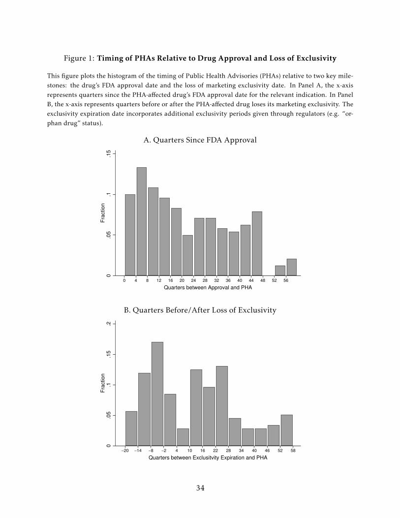
Figure 1: Timing of PHAs Relative to Drug Approval and Loss of Exclusivity

This figure plots the histogram of the timing of Public Health Advisories (PHAs) relative to two key mile-stones: the drug’s FDA approval date and the loss of marketing exclusivity date. In Panel A, the x-axisrepresents quarters since the PHA-affected drug’s FDA approval date for the relevant indication. In PanelB, the x-axis represents quarters before or after the PHA-affected drug loses its marketing exclusivity. Theexclusivity expiration date incorporates additional exclusivity periods given through regulators (e.g. “or-phan drug” status).

A. Quarters Since FDA Approval

0.0

5.1

.15

Fra

ction

0 4 8 12 16 20 24 28 32 36 40 44 48 52 56

Quarters between Approval and PHA

B. Quarters Before/After Loss of Exclusivity

0.0

5.1

.15

.2F

raction

−20 −14 −8 −2 4 10 16 22 28 34 40 46 52 58

Quarters between Exclusitvity Expiration and PHA

34

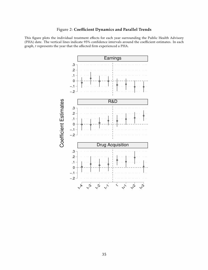
Figure 2: Coefficient Dynamics and Parallel Trends

This figure plots the individual treatment effects for each year surrounding the Public Health Advisory(PHA) date. The vertical lines indicate 95% confidence intervals around the coefficient estimates. In eachgraph, t represents the year that the affected firm experienced a PHA.

−.2

−.1

0

.1

.2

.3

−.2

−.1

0

.1

.2

.3

−.2

−.1

0

.1

.2

.3

t−4

t−3

t−2

t−1 t

t+1

t+2

t+3

Earnings

R&D

Drug AcquisitionCo

eff

icie

nt

Estim

ate

s

35

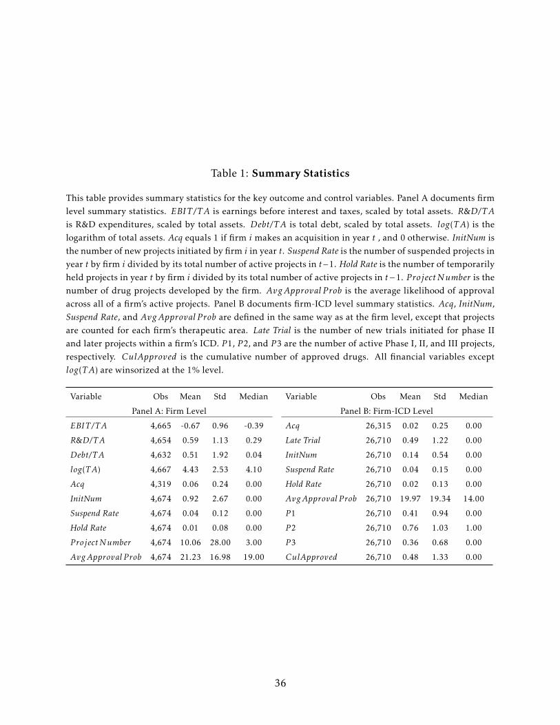
Table 1: Summary Statistics

This table provides summary statistics for the key outcome and control variables. Panel A documents firmlevel summary statistics. EBIT /T A is earnings before interest and taxes, scaled by total assets. R&D/TAis R&D expenditures, scaled by total assets. Debt/T A is total debt, scaled by total assets. log(TA) is thelogarithm of total assets. Acq equals 1 if firm i makes an acquisition in year t , and 0 otherwise. InitNum isthe number of new projects initiated by firm i in year t. Suspend Rate is the number of suspended projects inyear t by firm i divided by its total number of active projects in t−1. Hold Rate is the number of temporarilyheld projects in year t by firm i divided by its total number of active projects in t−1. P rojectNumber is thenumber of drug projects developed by the firm. AvgApproval P rob is the average likelihood of approvalacross all of a firm’s active projects. Panel B documents firm-ICD level summary statistics. Acq, InitNum,Suspend Rate, and AvgApproval P rob are defined in the same way as at the firm level, except that projectsare counted for each firm’s therapeutic area. Late Trial is the number of new trials initiated for phase IIand later projects within a firm’s ICD. P 1, P 2, and P 3 are the number of active Phase I, II, and III projects,respectively. CulApproved is the cumulative number of approved drugs. All financial variables exceptlog(TA) are winsorized at the 1% level.

Variable Obs Mean Std Median Variable Obs Mean Std Median

Panel A: Firm Level Panel B: Firm-ICD Level

EBIT /T A 4,665 -0.67 0.96 -0.39 Acq 26,315 0.02 0.25 0.00

R&D/TA 4,654 0.59 1.13 0.29 Late Trial 26,710 0.49 1.22 0.00

Debt/T A 4,632 0.51 1.92 0.04 InitNum 26,710 0.14 0.54 0.00

log(TA) 4,667 4.43 2.53 4.10 Suspend Rate 26,710 0.04 0.15 0.00

Acq 4,319 0.06 0.24 0.00 Hold Rate 26,710 0.02 0.13 0.00

InitNum 4,674 0.92 2.67 0.00 AvgApproval P rob 26,710 19.97 19.34 14.00

Suspend Rate 4,674 0.04 0.12 0.00 P 1 26,710 0.41 0.94 0.00

Hold Rate 4,674 0.01 0.08 0.00 P 2 26,710 0.76 1.03 1.00

P rojectNumber 4,674 10.06 28.00 3.00 P 3 26,710 0.36 0.68 0.00

AvgApproval P rob 4,674 21.23 16.98 19.00 CulApproved 26,710 0.48 1.33 0.00

36

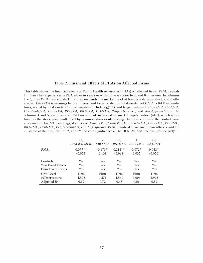
Table 2: Financial Effects of PHAs on Affected Firms

This table shows the financial effects of Public Health Advisories (PHAs) on affected firms. PHAi,t equals1 if firm i has experienced a PHA either in year t or within 3 years prior to it, and 0 otherwise. In columns1 – 3, P rodW ithdraw equals 1 if a firm suspends the marketing of at least one drug product, and 0 oth-erwise. EBIT /T A is earnings before interest and taxes, scaled by total assets. R&D/TA is R&D expendi-tures, scaled by total assets. Control variables include log(TA), and lagged values of: Capex/T A, Cash/T A,Dividends/T A, EBIT /T A, P P E/T A, R&D/TA, Debt/T A, P rojectNumber, and AvgApproval P rob. Incolumns 4 and 5, earnings and R&D investment are scaled by market capitalization (MC), which is de-fined as the stock price multiplied by common shares outstanding. In these columns, the control vari-ables include log(MC), and lagged values of: Capex/MC, Cash/MC, Dividends/MC, EBIT /MC, P P E/MC,R&D/MC, Debt/MC, P rojectNumber, and AvgApproval P rob. Standard errors are in parentheses, and areclustered at the firm level. *, **, and *** indicate significance at the 10%, 5%, and 1% level, respectively.

(1) (2) (3) (4) (5)P rodW ithdraw EBIT /T A R&D/TA EBIT /MC R&D/MC

PHAi,t 0.077*** -0.178** 0.214*** -0.072** 0.042**(0.024) (0.138) (0.068) (0.035) (0.020)

Controls Yes Yes Yes Yes YesYear Fixed Effects Yes Yes Yes Yes YesFirm Fixed Effects Yes Yes Yes Yes YesUnit Level Firm Firm Firm Firm Firm#Observations 4,573 4,571 4,560 4,006 3,995Adjusted R2 0.12 0.72 0.48 0.56 0.52

37

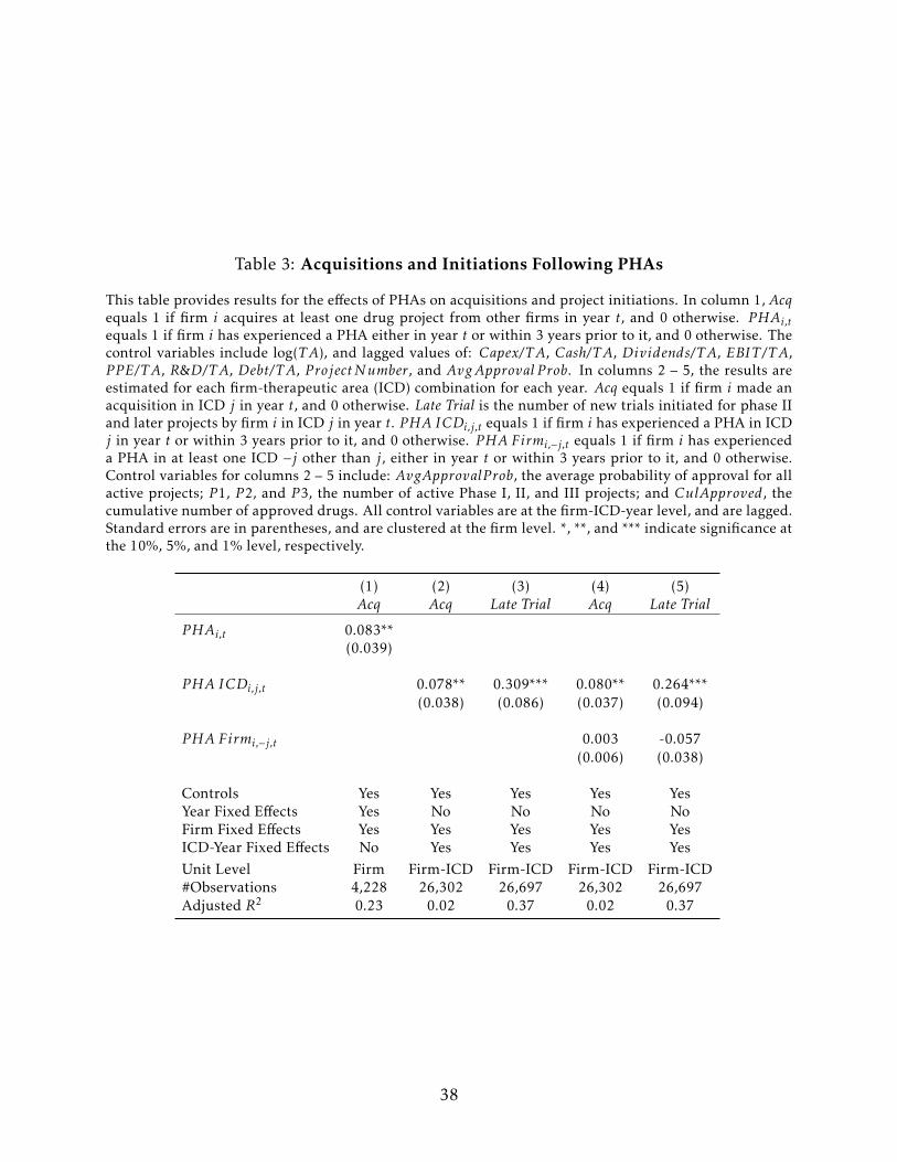
Table 3: Acquisitions and Initiations Following PHAs

This table provides results for the effects of PHAs on acquisitions and project initiations. In column 1, Acqequals 1 if firm i acquires at least one drug project from other firms in year t, and 0 otherwise. PHAi,tequals 1 if firm i has experienced a PHA either in year t or within 3 years prior to it, and 0 otherwise. Thecontrol variables include log(TA), and lagged values of: Capex/T A, Cash/T A, Dividends/T A, EBIT /T A,P P E/T A, R&D/TA, Debt/T A, P rojectNumber, and AvgApproval P rob. In columns 2 – 5, the results areestimated for each firm-therapeutic area (ICD) combination for each year. Acq equals 1 if firm i made anacquisition in ICD j in year t, and 0 otherwise. Late Trial is the number of new trials initiated for phase IIand later projects by firm i in ICD j in year t. PHA ICDi,j,t equals 1 if firm i has experienced a PHA in ICDj in year t or within 3 years prior to it, and 0 otherwise. PHA Firmi,−j,t equals 1 if firm i has experienceda PHA in at least one ICD −j other than j, either in year t or within 3 years prior to it, and 0 otherwise.Control variables for columns 2 – 5 include: AvgApprovalP rob, the average probability of approval for allactive projects; P 1, P 2, and P 3, the number of active Phase I, II, and III projects; and CulApproved, thecumulative number of approved drugs. All control variables are at the firm-ICD-year level, and are lagged.Standard errors are in parentheses, and are clustered at the firm level. *, **, and *** indicate significance atthe 10%, 5%, and 1% level, respectively.

(1) (2) (3) (4) (5)Acq Acq Late Trial Acq Late Trial

PHAi,t 0.083**(0.039)

PHA ICDi,j,t 0.078** 0.309*** 0.080** 0.264***(0.038) (0.086) (0.037) (0.094)

PHA Firmi,−j,t 0.003 -0.057(0.006) (0.038)

Controls Yes Yes Yes Yes YesYear Fixed Effects Yes No No No NoFirm Fixed Effects Yes Yes Yes Yes YesICD-Year Fixed Effects No Yes Yes Yes YesUnit Level Firm Firm-ICD Firm-ICD Firm-ICD Firm-ICD#Observations 4,228 26,302 26,697 26,302 26,697Adjusted R2 0.23 0.02 0.37 0.02 0.37

38

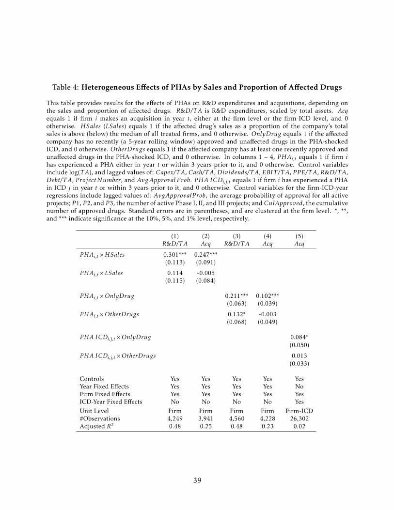
Table 4: Heterogeneous Effects of PHAs by Sales and Proportion of Affected Drugs

This table provides results for the effects of PHAs on R&D expenditures and acquisitions, depending onthe sales and proportion of affected drugs. R&D/TA is R&D expenditures, scaled by total assets. Acqequals 1 if firm i makes an acquisition in year t, either at the firm level or the firm-ICD level, and 0otherwise. HSales (LSales) equals 1 if the affected drug’s sales as a proportion of the company’s totalsales is above (below) the median of all treated firms, and 0 otherwise. OnlyDrug equals 1 if the affectedcompany has no recently (a 5-year rolling window) approved and unaffected drugs in the PHA-shockedICD, and 0 otherwise. OtherDrugs equals 1 if the affected company has at least one recently approved andunaffected drugs in the PHA-shocked ICD, and 0 otherwise. In columns 1 – 4, PHAi,t equals 1 if firm ihas experienced a PHA either in year t or within 3 years prior to it, and 0 otherwise. Control variablesinclude log(TA), and lagged values of: Capex/T A, Cash/T A, Dividends/T A, EBIT /T A, P P E/T A, R&D/TA,Debt/T A, P rojectNumber, and AvgApproval P rob. PHA ICDi,j,t equals 1 if firm i has experienced a PHAin ICD j in year t or within 3 years prior to it, and 0 otherwise. Control variables for the firm-ICD-yearregressions include lagged values of: AvgApprovalP rob, the average probability of approval for all activeprojects; P 1, P 2, and P 3, the number of active Phase I, II, and III projects; andCulApproved, the cumulativenumber of approved drugs. Standard errors are in parentheses, and are clustered at the firm level. *, **,and *** indicate significance at the 10%, 5%, and 1% level, respectively.

(1) (2) (3) (4) (5)R&D/TA Acq R&D/TA Acq Acq

PHAi,t ×HSales 0.301*** 0.247***(0.113) (0.091)

PHAi,t ×LSales 0.114 -0.005(0.115) (0.084)

PHAi,t ×OnlyDrug 0.211*** 0.102***(0.063) (0.039)

PHAi,t ×OtherDrugs 0.132* -0.003(0.068) (0.049)

PHA ICDi,j,t ×OnlyDrug 0.084*(0.050)

PHA ICDi,j,t ×OtherDrugs 0.013(0.033)

Controls Yes Yes Yes Yes YesYear Fixed Effects Yes Yes Yes Yes NoFirm Fixed Effects Yes Yes Yes Yes YesICD-Year Fixed Effects No No No No YesUnit Level Firm Firm Firm Firm Firm-ICD#Observations 4,249 3,941 4,560 4,228 26,302Adjusted R2 0.48 0.25 0.48 0.23 0.02

39

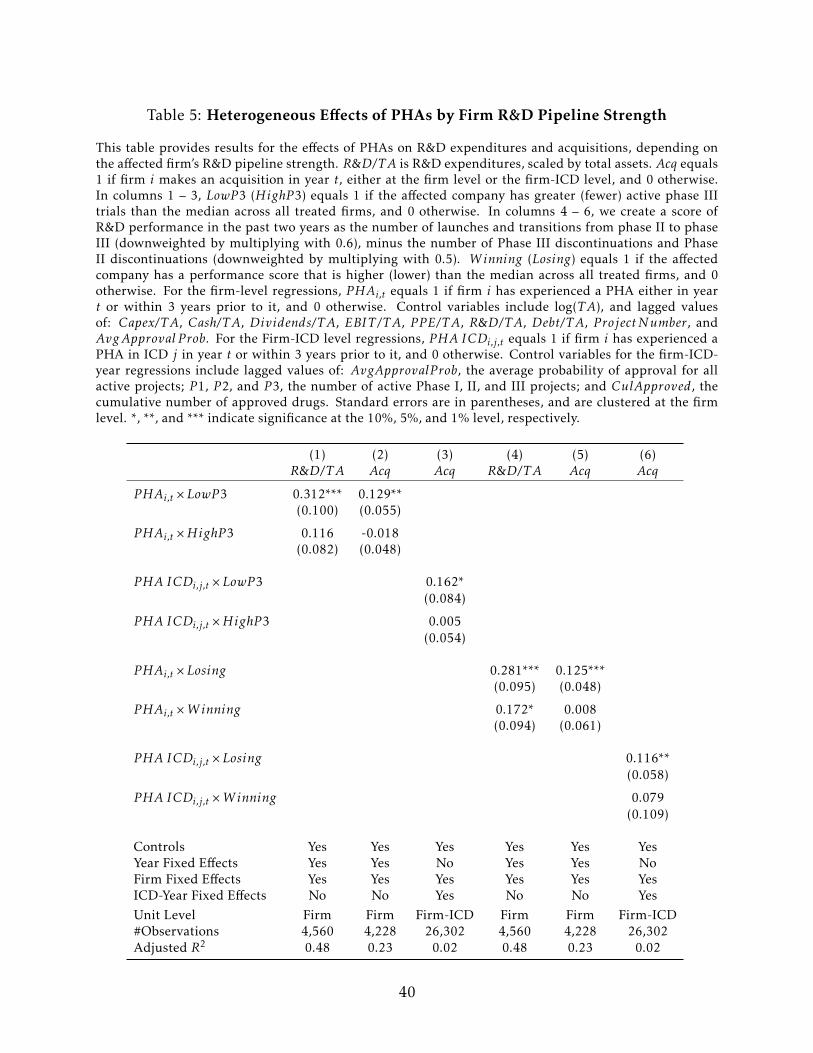
Table 5: Heterogeneous Effects of PHAs by Firm R&D Pipeline Strength

This table provides results for the effects of PHAs on R&D expenditures and acquisitions, depending onthe affected firm’s R&D pipeline strength. R&D/TA is R&D expenditures, scaled by total assets. Acq equals1 if firm i makes an acquisition in year t, either at the firm level or the firm-ICD level, and 0 otherwise.In columns 1 – 3, LowP 3 (HighP 3) equals 1 if the affected company has greater (fewer) active phase IIItrials than the median across all treated firms, and 0 otherwise. In columns 4 – 6, we create a score ofR&D performance in the past two years as the number of launches and transitions from phase II to phaseIII (downweighted by multiplying with 0.6), minus the number of Phase III discontinuations and PhaseII discontinuations (downweighted by multiplying with 0.5). Winning (Losing) equals 1 if the affectedcompany has a performance score that is higher (lower) than the median across all treated firms, and 0otherwise. For the firm-level regressions, PHAi,t equals 1 if firm i has experienced a PHA either in yeart or within 3 years prior to it, and 0 otherwise. Control variables include log(TA), and lagged valuesof: Capex/T A, Cash/T A, Dividends/T A, EBIT /T A, P P E/T A, R&D/TA, Debt/T A, P rojectNumber, andAvgApproval P rob. For the Firm-ICD level regressions, PHA ICDi,j,t equals 1 if firm i has experienced aPHA in ICD j in year t or within 3 years prior to it, and 0 otherwise. Control variables for the firm-ICD-year regressions include lagged values of: AvgApprovalP rob, the average probability of approval for allactive projects; P 1, P 2, and P 3, the number of active Phase I, II, and III projects; and CulApproved, thecumulative number of approved drugs. Standard errors are in parentheses, and are clustered at the firmlevel. *, **, and *** indicate significance at the 10%, 5%, and 1% level, respectively.

(1) (2) (3) (4) (5) (6)R&D/TA Acq Acq R&D/TA Acq Acq

PHAi,t ×LowP 3 0.312*** 0.129**(0.100) (0.055)

PHAi,t ×HighP 3 0.116 -0.018(0.082) (0.048)

PHA ICDi,j,t ×LowP 3 0.162*(0.084)

PHA ICDi,j,t ×HighP 3 0.005(0.054)

PHAi,t ×Losing 0.281*** 0.125***(0.095) (0.048)

PHAi,t ×Winning 0.172* 0.008(0.094) (0.061)

PHA ICDi,j,t ×Losing 0.116**(0.058)

PHA ICDi,j,t ×Winning 0.079(0.109)

Controls Yes Yes Yes Yes Yes YesYear Fixed Effects Yes Yes No Yes Yes NoFirm Fixed Effects Yes Yes Yes Yes Yes YesICD-Year Fixed Effects No No Yes No No YesUnit Level Firm Firm Firm-ICD Firm Firm Firm-ICD#Observations 4,560 4,228 26,302 4,560 4,228 26,302Adjusted R2 0.48 0.23 0.02 0.48 0.23 0.02

40

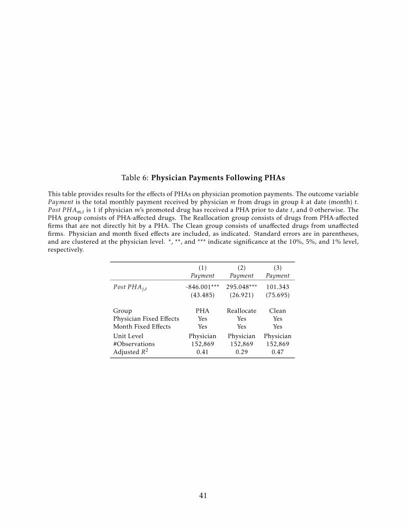
Table 6: Physician Payments Following PHAs

This table provides results for the effects of PHAs on physician promotion payments. The outcome variableP ayment is the total monthly payment received by physician m from drugs in group k at date (month) t.P ost PHAm,t is 1 if physician m’s promoted drug has received a PHA prior to date t, and 0 otherwise. ThePHA group consists of PHA-affected drugs. The Reallocation group consists of drugs from PHA-affectedfirms that are not directly hit by a PHA. The Clean group consists of unaffected drugs from unaffectedfirms. Physician and month fixed effects are included, as indicated. Standard errors are in parentheses,and are clustered at the physician level. *, **, and *** indicate significance at the 10%, 5%, and 1% level,respectively.

(1) (2) (3)Payment Payment Payment

P ost PHAj,t -846.001*** 295.048*** 101.343(43.485) (26.921) (75.695)

Group PHA Reallocate CleanPhysician Fixed Effects Yes Yes YesMonth Fixed Effects Yes Yes YesUnit Level Physician Physician Physician#Observations 152,869 152,869 152,869Adjusted R2 0.41 0.29 0.47

41

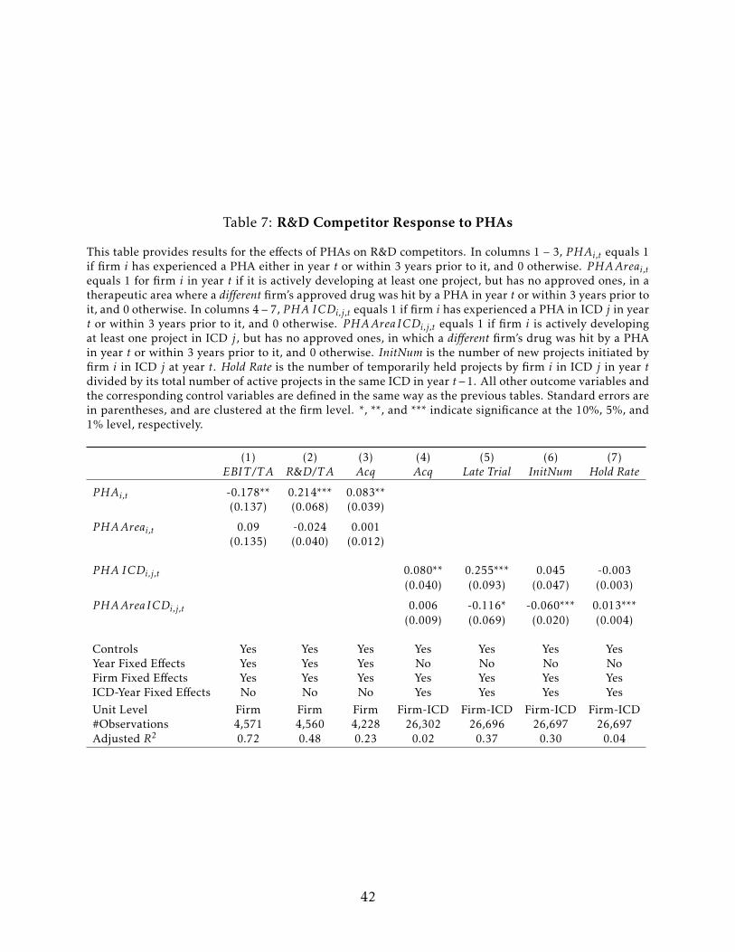
Table 7: R&D Competitor Response to PHAs

This table provides results for the effects of PHAs on R&D competitors. In columns 1 – 3, PHAi,t equals 1if firm i has experienced a PHA either in year t or within 3 years prior to it, and 0 otherwise. PHAAreai,tequals 1 for firm i in year t if it is actively developing at least one project, but has no approved ones, in atherapeutic area where a different firm’s approved drug was hit by a PHA in year t or within 3 years prior toit, and 0 otherwise. In columns 4 – 7, PHA ICDi,j,t equals 1 if firm i has experienced a PHA in ICD j in yeart or within 3 years prior to it, and 0 otherwise. PHAAreaICDi,j,t equals 1 if firm i is actively developingat least one project in ICD j, but has no approved ones, in which a different firm’s drug was hit by a PHAin year t or within 3 years prior to it, and 0 otherwise. InitNum is the number of new projects initiated byfirm i in ICD j at year t. Hold Rate is the number of temporarily held projects by firm i in ICD j in year tdivided by its total number of active projects in the same ICD in year t−1. All other outcome variables andthe corresponding control variables are defined in the same way as the previous tables. Standard errors arein parentheses, and are clustered at the firm level. *, **, and *** indicate significance at the 10%, 5%, and1% level, respectively.

(1) (2) (3) (4) (5) (6) (7)EBIT /T A R&D/TA Acq Acq Late Trial InitNum Hold Rate

PHAi,t -0.178** 0.214*** 0.083**(0.137) (0.068) (0.039)

PHAAreai,t 0.09 -0.024 0.001(0.135) (0.040) (0.012)

PHA ICDi,j,t 0.080** 0.255*** 0.045 -0.003(0.040) (0.093) (0.047) (0.003)

PHAAreaICDi,j,t 0.006 -0.116* -0.060*** 0.013***(0.009) (0.069) (0.020) (0.004)

Controls Yes Yes Yes Yes Yes Yes YesYear Fixed Effects Yes Yes Yes No No No NoFirm Fixed Effects Yes Yes Yes Yes Yes Yes YesICD-Year Fixed Effects No No No Yes Yes Yes YesUnit Level Firm Firm Firm Firm-ICD Firm-ICD Firm-ICD Firm-ICD#Observations 4,571 4,560 4,228 26,302 26,696 26,697 26,697Adjusted R2 0.72 0.48 0.23 0.02 0.37 0.30 0.04

42

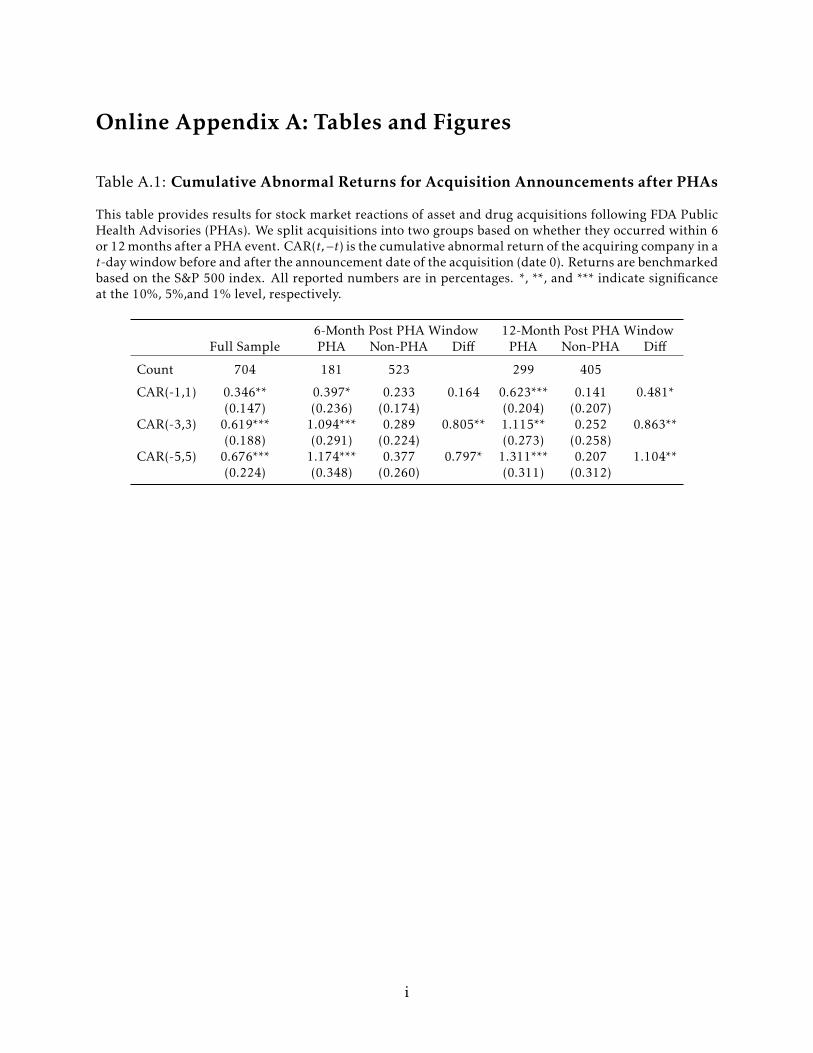
Online Appendix A: Tables and Figures

Table A.1: Cumulative Abnormal Returns for Acquisition Announcements after PHAs

This table provides results for stock market reactions of asset and drug acquisitions following FDA PublicHealth Advisories (PHAs). We split acquisitions into two groups based on whether they occurred within 6or 12 months after a PHA event. CAR(t,−t) is the cumulative abnormal return of the acquiring company in at-day window before and after the announcement date of the acquisition (date 0). Returns are benchmarkedbased on the S&P 500 index. All reported numbers are in percentages. *, **, and *** indicate significanceat the 10%, 5%,and 1% level, respectively.

6-Month Post PHA Window 12-Month Post PHA WindowFull Sample PHA Non-PHA Diff PHA Non-PHA Diff

Count 704 181 523 299 405

CAR(-1,1) 0.346** 0.397* 0.233 0.164 0.623*** 0.141 0.481*(0.147) (0.236) (0.174) (0.204) (0.207)

CAR(-3,3) 0.619*** 1.094*** 0.289 0.805** 1.115** 0.252 0.863**(0.188) (0.291) (0.224) (0.273) (0.258)

CAR(-5,5) 0.676*** 1.174*** 0.377 0.797* 1.311*** 0.207 1.104**(0.224) (0.348) (0.260) (0.311) (0.312)

i

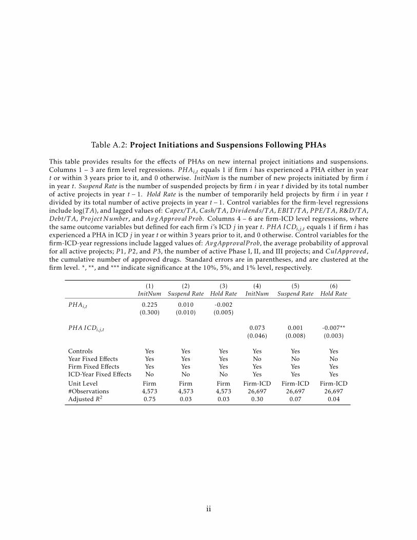
Table A.2: Project Initiations and Suspensions Following PHAs

This table provides results for the effects of PHAs on new internal project initiations and suspensions.Columns 1 – 3 are firm level regressions. PHAi,t equals 1 if firm i has experienced a PHA either in yeart or within 3 years prior to it, and 0 otherwise. InitNum is the number of new projects initiated by firm iin year t. Suspend Rate is the number of suspended projects by firm i in year t divided by its total numberof active projects in year t − 1. Hold Rate is the number of temporarily held projects by firm i in year tdivided by its total number of active projects in year t − 1. Control variables for the firm-level regressionsinclude log(TA), and lagged values of: Capex/T A, Cash/T A, Dividends/T A, EBIT /T A, P P E/T A, R&D/TA,Debt/T A, P rojectNumber, and AvgApproval P rob. Columns 4 – 6 are firm-ICD level regressions, wherethe same outcome variables but defined for each firm i’s ICD j in year t. PHA ICDi,j,t equals 1 if firm i hasexperienced a PHA in ICD j in year t or within 3 years prior to it, and 0 otherwise. Control variables for thefirm-ICD-year regressions include lagged values of: AvgApprovalP rob, the average probability of approvalfor all active projects; P 1, P 2, and P 3, the number of active Phase I, II, and III projects; and CulApproved,the cumulative number of approved drugs. Standard errors are in parentheses, and are clustered at thefirm level. *, **, and *** indicate significance at the 10%, 5%, and 1% level, respectively.

(1) (2) (3) (4) (5) (6)InitNum Suspend Rate Hold Rate InitNum Suspend Rate Hold Rate

PHAi,t 0.225 0.010 -0.002(0.300) (0.010) (0.005)

PHA ICDi,j,t 0.073 0.001 -0.007**(0.046) (0.008) (0.003)

Controls Yes Yes Yes Yes Yes YesYear Fixed Effects Yes Yes Yes No No NoFirm Fixed Effects Yes Yes Yes Yes Yes YesICD-Year Fixed Effects No No No Yes Yes YesUnit Level Firm Firm Firm Firm-ICD Firm-ICD Firm-ICD#Observations 4,573 4,573 4,573 26,697 26,697 26,697Adjusted R2 0.75 0.03 0.03 0.30 0.07 0.04

ii

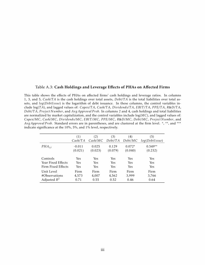
Table A.3: Cash Holdings and Leverage Effects of PHAs on Affected Firms

This table shows the effects of PHAs on affected firms’ cash holdings and leverage ratios. In columns1, 3, and 5, Cash/T A is the cash holdings over total assets, Debt/T A is the total liabilities over total as-sets, and log(DebtIssue) is the logarithm of debt issuance. In these columns, the control variables in-clude log(TA), and lagged values of: Capex/T A, Cash/T A, Dividends/T A, EBIT /T A, P P E/T A, R&D/TA,Debt/T A, P rojectNumber, and AvgApproval P rob. In columns 2 and 4, cash holdings and total liabilitiesare normalized by market capitalization, and the control variables include log(MC), and lagged values of:Capex/MC, Cash/MC, Dividends/MC, EBIT /MC, P P E/MC, R&D/MC, Debt/MC, P rojectNumber, andAvgApproval P rob. Standard errors are in parentheses, and are clustered at the firm level. *, **, and ***indicate significance at the 10%, 5%, and 1% level, respectively.

(1) (2) (3) (4) (5)Cash/T A Cash/MC Debt/T A Debt/MC log(DebtIssue)

PHAi,t -0.011 0.025 0.129 0.072* 0.549**(0.021) (0.023) (0.079) (0.040) (0.232)

Controls Yes Yes Yes Yes YesYear Fixed Effects Yes Yes Yes Yes YesFirm Fixed Effects Yes Yes Yes Yes YesUnit Level Firm Firm Firm Firm Firm#Observations 4,573 4,007 4,562 3,999 3,766Adjusted R2 0.71 0.55 0.52 0.46 0.64

iii

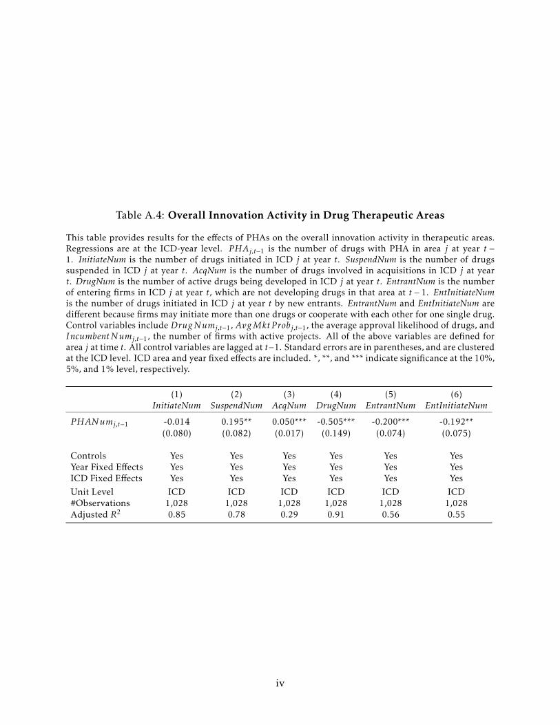
Table A.4: Overall Innovation Activity in Drug Therapeutic Areas

This table provides results for the effects of PHAs on the overall innovation activity in therapeutic areas.Regressions are at the ICD-year level. PHAj,t−1 is the number of drugs with PHA in area j at year t −1. InitiateNum is the number of drugs initiated in ICD j at year t. SuspendNum is the number of drugssuspended in ICD j at year t. AcqNum is the number of drugs involved in acquisitions in ICD j at yeart. DrugNum is the number of active drugs being developed in ICD j at year t. EntrantNum is the numberof entering firms in ICD j at year t, which are not developing drugs in that area at t − 1. EntInitiateNumis the number of drugs initiated in ICD j at year t by new entrants. EntrantNum and EntInitiateNum aredifferent because firms may initiate more than one drugs or cooperate with each other for one single drug.Control variables include DrugNumj,t−1, AvgMkt P robj,t−1, the average approval likelihood of drugs, andIncumbentNumj,t−1, the number of firms with active projects. All of the above variables are defined forarea j at time t. All control variables are lagged at t−1. Standard errors are in parentheses, and are clusteredat the ICD level. ICD area and year fixed effects are included. *, **, and *** indicate significance at the 10%,5%, and 1% level, respectively.

(1) (2) (3) (4) (5) (6)InitiateNum SuspendNum AcqNum DrugNum EntrantNum EntInitiateNum

PHANumj,t−1 -0.014 0.195** 0.050*** -0.505*** -0.200*** -0.192**(0.080) (0.082) (0.017) (0.149) (0.074) (0.075)

Controls Yes Yes Yes Yes Yes YesYear Fixed Effects Yes Yes Yes Yes Yes YesICD Fixed Effects Yes Yes Yes Yes Yes YesUnit Level ICD ICD ICD ICD ICD ICD#Observations 1,028 1,028 1,028 1,028 1,028 1,028Adjusted R2 0.85 0.78 0.29 0.91 0.56 0.55

iv

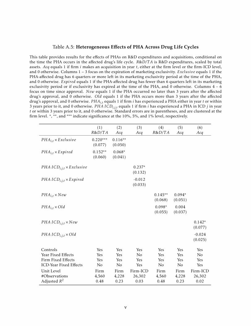
Table A.5: Heterogeneous Effects of PHA Across Drug Life Cycles

This table provides results for the effects of PHAs on R&D expenditures and acquisitions, conditional onthe time the PHA occurs in the affected drug’s life cycle. R&D/TA is R&D expenditures, scaled by totalassets. Acq equals 1 if firm i makes an acquisition in year t, either at the firm level or the firm-ICD level,and 0 otherwise. Columns 1 – 3 focus on the expiration of marketing exclusivity. Exclusive equals 1 if thePHA-affected drug has 6 quarters or more left in its marketing exclusivity period at the time of the PHA,and 0 otherwise. Expired equals 1 if the PHA-affected drug has fewer than 6 quarters left in its marketingexclusivity period or if exclusivity has expired at the time of the PHA, and 0 otherwise. Columns 4 – 6focus on time since approval. New equals 1 if the PHA occurred no later than 3 years after the affecteddrug’s approval, and 0 otherwise. Old equals 1 if the PHA occurs more than 3 years after the affecteddrug’s approval, and 0 otherwise. PHAi,t equals 1 if firm i has experienced a PHA either in year t or within3 years prior to it, and 0 otherwise. PHA ICDi,j,t equals 1 if firm i has experienced a PHA in ICD j in yeart or within 3 years prior to it, and 0 otherwise. Standard errors are in parentheses, and are clustered at thefirm level. *, **, and *** indicate significance at the 10%, 5%, and 1% level, respectively.

(1) (2) (3) (4) (5) (6)R&D/TA Acq Acq R&D/TA Acq Acq

PHAi,t ×Exclusive 0.220*** 0.116**(0.077) (0.050)

PHAi,t ×Expired 0.152** 0.068*(0.060) (0.041)

PHA ICDi,j,t ×Exclusive 0.237*(0.132)

PHA ICDi,j,t ×Expired -0.012(0.033)

PHAi,t ×New 0.145** 0.094*(0.068) (0.051)

PHAi,t ×Old 0.098* 0.004(0.055) (0.037)

PHA ICDi,j,t ×New 0.142*(0.077)

PHA ICDi,j,t ×Old -0.024(0.025)

Controls Yes Yes Yes Yes Yes YesYear Fixed Effects Yes Yes No Yes Yes NoFirm Fixed Effects Yes Yes Yes Yes Yes YesICD-Year Fixed Effects No No Yes No No YesUnit Level Firm Firm Firm-ICD Firm Firm Firm-ICD#Observations 4,560 4,228 26,302 4,560 4,228 26,302Adjusted R2 0.48 0.23 0.03 0.48 0.23 0.02

v

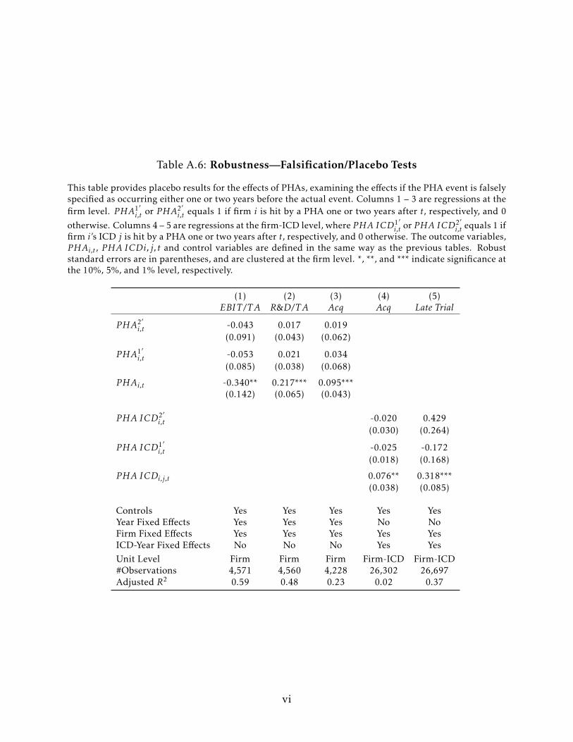
Table A.6: Robustness—Falsification/Placebo Tests

This table provides placebo results for the effects of PHAs, examining the effects if the PHA event is falselyspecified as occurring either one or two years before the actual event. Columns 1 – 3 are regressions at thefirm level. PHA1′

i,t or PHA2′i,t equals 1 if firm i is hit by a PHA one or two years after t, respectively, and 0

otherwise. Columns 4 – 5 are regressions at the firm-ICD level, where PHA ICD1′i,t or PHA ICD2′

i,t equals 1 iffirm i’s ICD j is hit by a PHA one or two years after t, respectively, and 0 otherwise. The outcome variables,PHAi,t , PHA ICDi, j, t and control variables are defined in the same way as the previous tables. Robuststandard errors are in parentheses, and are clustered at the firm level. *, **, and *** indicate significance atthe 10%, 5%, and 1% level, respectively.

(1) (2) (3) (4) (5)EBIT /T A R&D/TA Acq Acq Late Trial

PHA2′i,t -0.043 0.017 0.019

(0.091) (0.043) (0.062)

PHA1′i,t -0.053 0.021 0.034

(0.085) (0.038) (0.068)

PHAi,t -0.340** 0.217*** 0.095***(0.142) (0.065) (0.043)

PHA ICD2′i,t -0.020 0.429

(0.030) (0.264)

PHA ICD1′i,t -0.025 -0.172

(0.018) (0.168)

PHA ICDi,j,t 0.076** 0.318***(0.038) (0.085)

Controls Yes Yes Yes Yes YesYear Fixed Effects Yes Yes Yes No NoFirm Fixed Effects Yes Yes Yes Yes YesICD-Year Fixed Effects No No No Yes YesUnit Level Firm Firm Firm Firm-ICD Firm-ICD#Observations 4,571 4,560 4,228 26,302 26,697Adjusted R2 0.59 0.48 0.23 0.02 0.37

vi

Table A.7: Robustness—Propensity Score Matching

This table provides robustness results for the effects of PHAs, using propensity score matching to constructthe control group. R&D/TA is R&D expenditures, scaled by total assets. Acq equals 1 if firm i makes anacquisition in year t, either at the firm level or the firm-ICD level, and 0 otherwise. PHAi,t equals 1 if firmi has experienced a PHA either in year t or within 3 years prior to it, and 0 otherwise. PHA ICDi,j,t equals1 if firm i has experienced a PHA in ICD j in year t or within 3 years prior to it, and 0 otherwise. Standarderrors are in parentheses, and are clustered at the firm level. *, **, and *** indicate significance at the 10%,5%, and 1% level, respectively.

(1) (2) (3)R&D/TA Acq Acq

PHAi,t 0.079** 0.111**(0.032) (0.046)

PHA ICDi,j,t 0.090**(0.042)

Controls Yes Yes YesYear Fixed Effects Yes Yes NoFirm Fixed Effects Yes Yes YesICD-Year Fixed Effects No No YesUnit Level Firm Firm Firm-ICD#Observations 1,086 986 2,890Adjusted R2 0.38 0.17 0.01

vii

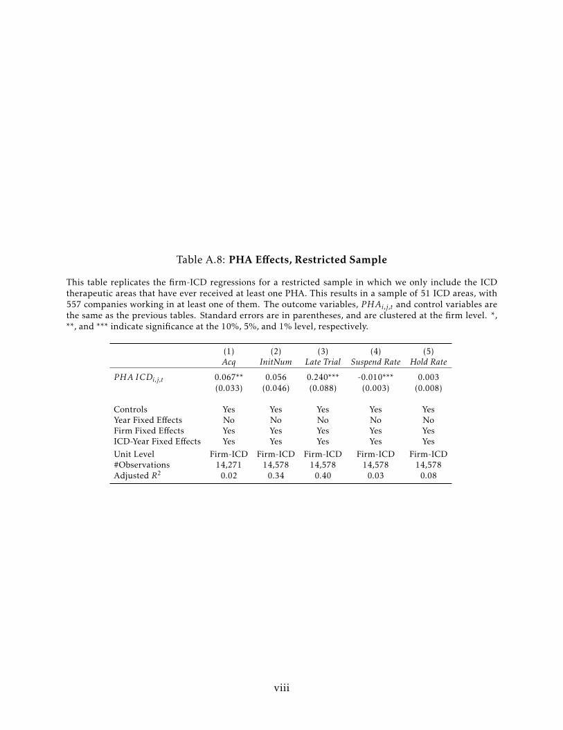
Table A.8: PHA Effects, Restricted Sample

This table replicates the firm-ICD regressions for a restricted sample in which we only include the ICDtherapeutic areas that have ever received at least one PHA. This results in a sample of 51 ICD areas, with557 companies working in at least one of them. The outcome variables, PHAi,j,t and control variables arethe same as the previous tables. Standard errors are in parentheses, and are clustered at the firm level. *,**, and *** indicate significance at the 10%, 5%, and 1% level, respectively.

(1) (2) (3) (4) (5)Acq InitNum Late Trial Suspend Rate Hold Rate

PHA ICDi,j,t 0.067** 0.056 0.240*** -0.010*** 0.003(0.033) (0.046) (0.088) (0.003) (0.008)

Controls Yes Yes Yes Yes YesYear Fixed Effects No No No No NoFirm Fixed Effects Yes Yes Yes Yes YesICD-Year Fixed Effects Yes Yes Yes Yes YesUnit Level Firm-ICD Firm-ICD Firm-ICD Firm-ICD Firm-ICD#Observations 14,271 14,578 14,578 14,578 14,578Adjusted R2 0.02 0.34 0.40 0.03 0.08

viii

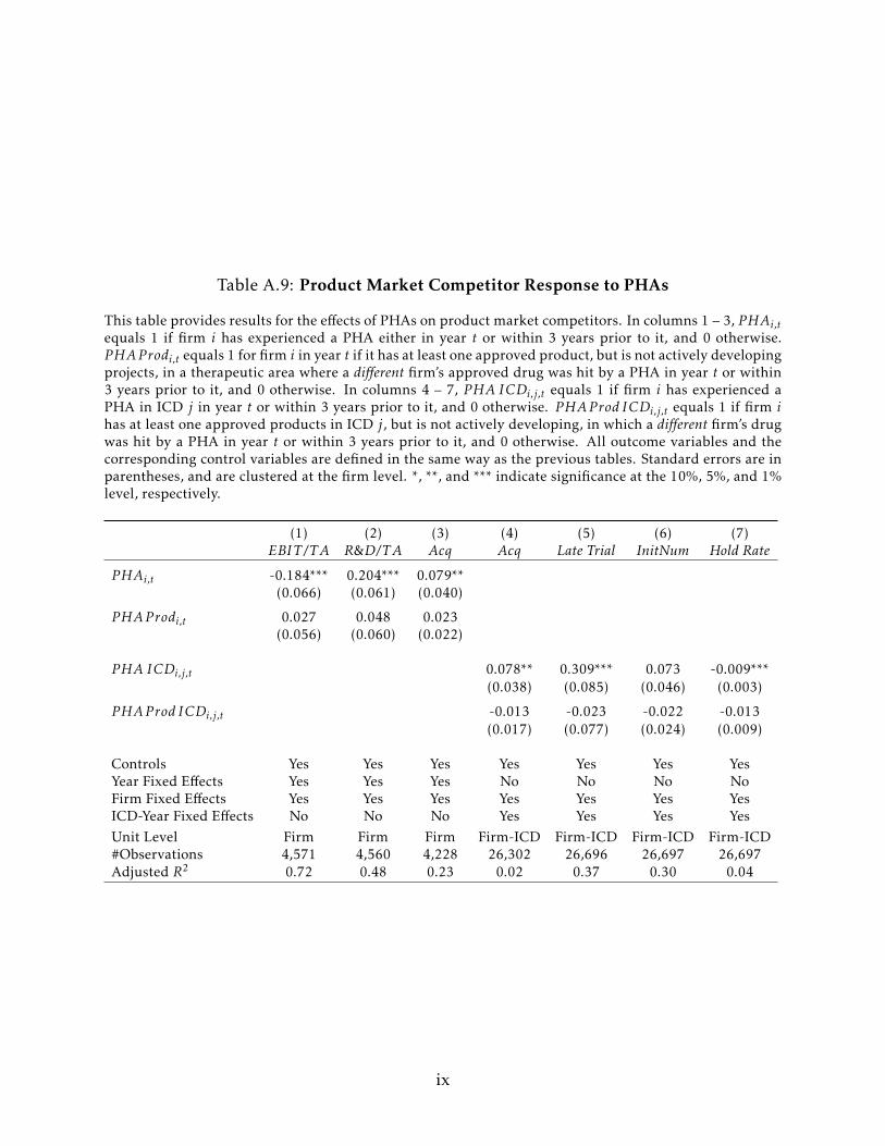
Table A.9: Product Market Competitor Response to PHAs

This table provides results for the effects of PHAs on product market competitors. In columns 1 – 3, PHAi,tequals 1 if firm i has experienced a PHA either in year t or within 3 years prior to it, and 0 otherwise.PHAP rodi,t equals 1 for firm i in year t if it has at least one approved product, but is not actively developingprojects, in a therapeutic area where a different firm’s approved drug was hit by a PHA in year t or within3 years prior to it, and 0 otherwise. In columns 4 – 7, PHA ICDi,j,t equals 1 if firm i has experienced aPHA in ICD j in year t or within 3 years prior to it, and 0 otherwise. PHAP rod ICDi,j,t equals 1 if firm ihas at least one approved products in ICD j, but is not actively developing, in which a different firm’s drugwas hit by a PHA in year t or within 3 years prior to it, and 0 otherwise. All outcome variables and thecorresponding control variables are defined in the same way as the previous tables. Standard errors are inparentheses, and are clustered at the firm level. *, **, and *** indicate significance at the 10%, 5%, and 1%level, respectively.

(1) (2) (3) (4) (5) (6) (7)EBIT /T A R&D/TA Acq Acq Late Trial InitNum Hold Rate

PHAi,t -0.184*** 0.204*** 0.079**(0.066) (0.061) (0.040)

PHAP rodi,t 0.027 0.048 0.023(0.056) (0.060) (0.022)

PHA ICDi,j,t 0.078** 0.309*** 0.073 -0.009***(0.038) (0.085) (0.046) (0.003)

PHAP rod ICDi,j,t -0.013 -0.023 -0.022 -0.013(0.017) (0.077) (0.024) (0.009)

Controls Yes Yes Yes Yes Yes Yes YesYear Fixed Effects Yes Yes Yes No No No NoFirm Fixed Effects Yes Yes Yes Yes Yes Yes YesICD-Year Fixed Effects No No No Yes Yes Yes YesUnit Level Firm Firm Firm Firm-ICD Firm-ICD Firm-ICD Firm-ICD#Observations 4,571 4,560 4,228 26,302 26,696 26,697 26,697Adjusted R2 0.72 0.48 0.23 0.02 0.37 0.30 0.04

ix

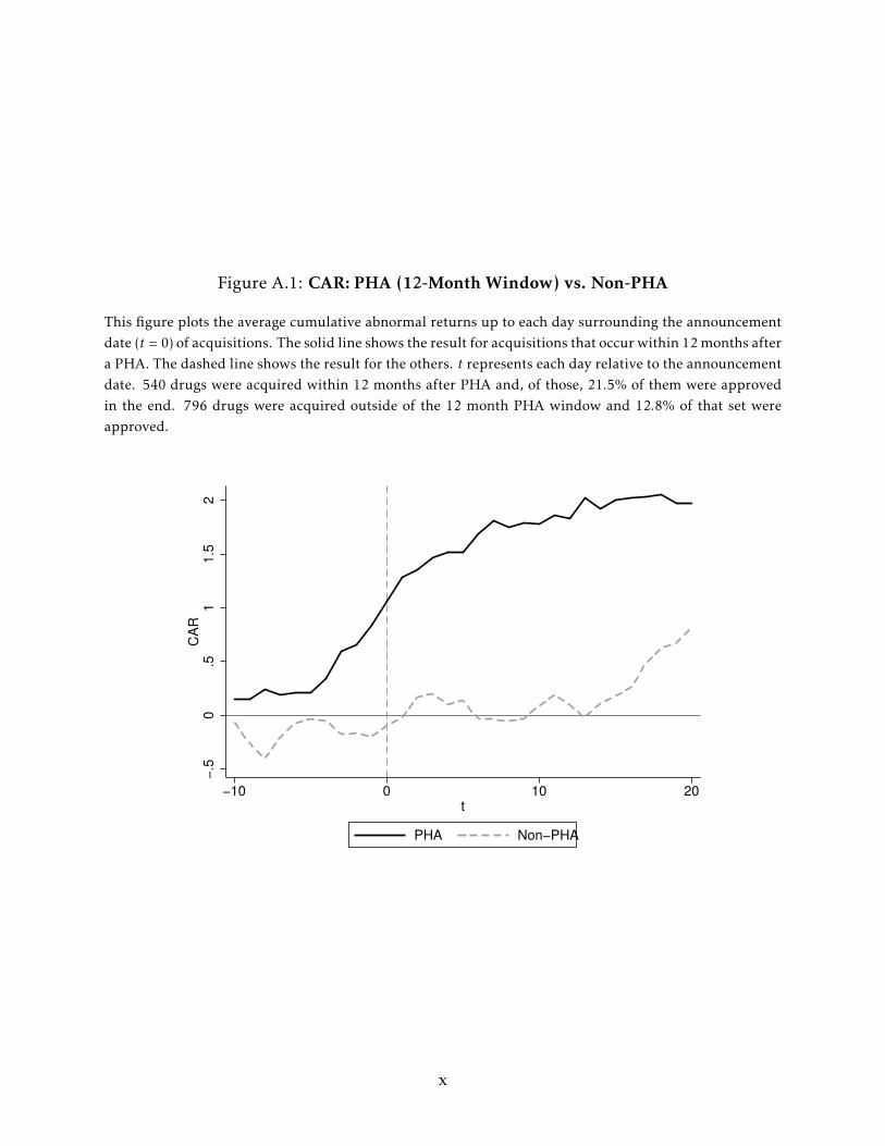
Figure A.1: CAR: PHA (12-Month Window) vs. Non-PHA

This figure plots the average cumulative abnormal returns up to each day surrounding the announcementdate (t = 0) of acquisitions. The solid line shows the result for acquisitions that occur within 12 months aftera PHA. The dashed line shows the result for the others. t represents each day relative to the announcementdate. 540 drugs were acquired within 12 months after PHA and, of those, 21.5% of them were approvedin the end. 796 drugs were acquired outside of the 12 month PHA window and 12.8% of that set wereapproved.

−.5

0.5

11

.52

CA

R

−10 0 10 20t

PHA Non−PHA

x

Online Appendix B: Model

B.1 Overview of Model

The model has four dates to capture two key phases of drug development: the R&D

and commercialization phases. In each of the two phases, the firm makes an endogenous

choice and the outcome at the end of each phase is uncertain.

In the first phase (first period of the model), the firm chooses the number of products

on which to do R&D. This involves early-stage clinical trials and related activities that

require both a fixed investment (independent of the number of products on which R&D

is being done), and a variable cost per product.

At the end of the first phase, the outcome of the R&D becomes known, so the firm

knows which products survived and which failed. The surviving products make it to the

second phase, which is the commercialization phase. The firm now chooses its aggregate

investment in commercialization capital, which then determines the value of the firm’s

downstream assets. This investment can be thought of as including the cost of late-stage

clinical trial infrastructure—recruiting, building relationships with medical centers and

doctors, sales and marketing, manufacturing and distribution channels, etc.

At the end of the second phase, the firm observes which products survived the com-

mercialization phase. The products that survive generate payoffs that depend on how

much the firm invested in commercialization. Although the firm chose its aggregate com-

mercialization capital investment at the start of the second phase, it has the flexibility to

(re)allocate this capital across the products that survive the second phase.

Also at the end of the second phase, one of the products may receive a Public Health

Advisory (PHA) shock, making the affected product worthless. The firm has the choice of

not doing anything in response to the shock, other than just dropping the affected prod-

uct, or it can replace the affected product by buying a similar product from a competing

firm. The competing firm has a product that has successfully made it through the first

i

phase of clinical trials, but has not yet been put through the commercialization phase.

So if the firm purchases this product, it can allocate to it the commercialization capital

vacated by the PHA-shocked product that is now abandoned. This fungability ensures

that the purchased product is simply allocated existing commercialization capital that

would have been otherwise simply spread out over the other products that survived the

purchasing firm’s second phase. The purchased product then goes through the commer-

cialization phase (with uncertainty about whether it will survive this phase).

Finally, in the third period, the payoffs on all the products that survived the second

phase are observed.

B.2 Baseline Setup

The model has three time periods across four dates, t = 0, 1, 2 and 3. For simplicity,

there is no discounting across periods. Consider a representative firm (hereafter “the

firm”) that engages in staged R&D .

In the first period at t = 0, the firm endogenously chooses the number of products to

develop through clinical trials, n ≥ 1. This requires a fixed R&D infrastructure cost of

R > 0 that is independent of n, and a variable cost ci for each project i, implying a total

cost of R+∑ni=1 ci . These investments at t = 0 allow the firm to set up the infrastructure for

R&D, which creates a value of V0 > 1 for each of the n products, conditional on the prod-

uct eventually being successfully commercialized. This value can be further enhanced

through investment in downstream assets as discussed below.

The outcome of the first R&D stage is uncertain at t = 0 and becomes known at t = 1, at

which time the firm observes how many of the n R&D projects survived. Let n1 denote the

(random) number of surviving projects. Viewed at t = 0, the distribution of n1 is: n1 = n

with probability 0.5 and n1 = n/2 with probability 0.5.45 After observing n1 at t = 1,

the firm determines its aggregate investment in commercialization capital/downstream

45This is perhaps the simplest specification of uncertainty about the outcome of early-stage research, toallow for parsimony in our specifications. Our results generalize to more complicated or general specifica-tions of outcome uncertainty.

ii

assets X.

The second period ends at t = 2, at which time the firm observes the random number of

projects, n2, that survive the commercialization phase. Viewed at t = 1, the distribution of

n2 is: n2 = n1 with probability S ∈ (0,1) and n2 = n1/2 with probability 1−S. Each product

generates a payoff of V (z) = V0 +V (z), where V (·) is a concavely increasing function of z,

the amount (i.e. commercialization capital) that the firm spends to successfully launch

the product. Due to concavity, the firm splits its aggregate commercialization capital X

evenly across the surviving projects, i.e. each gets z = X/n2. Thus, for a given n1, viewed at

t = 1 the distribution of V is V (X/n1) with probability S and V (X/ (n1/2)) with probability

1−S. The distribution of n2V (viewed at t = 1) is n1 [V0 +V (X/n1)] with probability S and

[n1/2][V0 +V (X/ (n1/2))] with probability 1− S.

We then introduce the Public Health Advisory (PHA) shock, which is a negative profit

shock to one of the firm’s products that occurs at t = 2. Specifically, with probability

α ∈ (0,1/2),46 one product (randomly picked by nature) of the n2 products suffers a PHA

shock. This shock makes the payoff on that product zero.

After the shock, the firm has two choices: it can do nothing (and simply reallocate the

commercialization capacity vacated by the abandoned product over the remaining prod-

ucts), or it can replace that product with another one that it buys from a seller it could

approach. The seller has one active project that has survived the first-stage R&D but has

not yet gone through the commercialization phase, i.e. in terms of its own timeline, the

product is at t = 1. The PHA-shocked firm endogenously chooses whether to make a

take-it-or-leave-it offer (TIOLI) to the seller and acquire this project.47 If the firm does

not purchase the replacement product, then it goes to the next period with n2 − 1 surviv-

ing products. If the firm acquires the product, then it is subject to the same uncertainty

in the commercialization phase as the firm’s other products, i.e. with probability S the

46This upper bound signifies that the probability of a PHA shock is bounded from above, which simplifiesthe proofs but is not necessary for our results.

47If the seller chooses to keep the project, it will invest downstream assets optimally given the sameV (z) = V0 +V (z).

iii

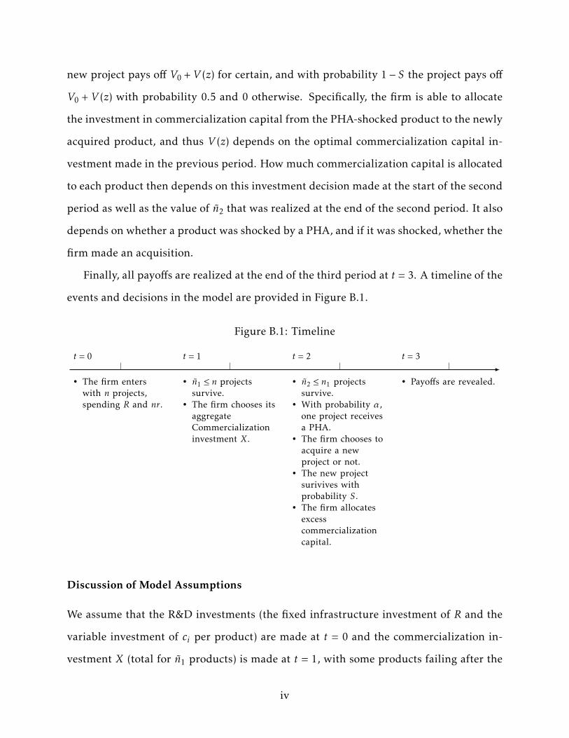
new project pays off V0 +V (z) for certain, and with probability 1− S the project pays off

V0 + V (z) with probability 0.5 and 0 otherwise. Specifically, the firm is able to allocate

the investment in commercialization capital from the PHA-shocked product to the newly

acquired product, and thus V (z) depends on the optimal commercialization capital in-

vestment made in the previous period. How much commercialization capital is allocated

to each product then depends on this investment decision made at the start of the second

period as well as the value of n2 that was realized at the end of the second period. It also

depends on whether a product was shocked by a PHA, and if it was shocked, whether the

firm made an acquisition.

Finally, all payoffs are realized at the end of the third period at t = 3. A timeline of the

events and decisions in the model are provided in Figure B.1.

Figure B.1: Timeline

• The firm enterswith n projects,spending R and nr.

• n1 ≤ n projectssurvive.

• The firm chooses itsaggregateCommercializationinvestment X.

• n2 ≤ n1 projectssurvive.

• With probability α,one project receivesa PHA.

• The firm chooses toacquire a newproject or not.

• The new projectsurivives withprobability S.

• The firm allocatesexcesscommercializationcapital.

• Payoffs are revealed.

t = 0 t = 1 t = 2 t = 3

Discussion of Model Assumptions

We assume that the R&D investments (the fixed infrastructure investment of R and the

variable investment of ci per product) are made at t = 0 and the commercialization in-

vestment X (total for n1 products) is made at t = 1, with some products failing after the

iv

R&D investment. Apart from the realism of the assumption in light of actual practice,

we make this assumption because we want to allow for the possibility that there is a firm

that has invested in R&D but not yet in commercialization, and that the PHA-shocked

firm can buy the product from such a firm. This makes it necessary to model these two

investments at two different points in time, and the possibility of post-R&D failures also

implies that it is optimal for the firm to wait until t = 1 and observe n1 before determining

X. We further assume that some firms experience product failures in the commercializa-

tion phase. This ensures heterogeneity among firms in terms of the strengths of their

product portfolios when they are hit with a PHA shock. We exploit this heterogeneity in

our empirical tests.

The firm’s payoff function, V , is assumed to be a concavely increasing function of its

investment in commercialization capital, and thus V′(z) > 0 and V

′′(z) < 0. Thus, invest-

ment in commercialization capital for products faces diminishing marginal returns to size

and scope. A number of realistic mechanisms can generate such diminishing returns as a

firm increases size and scope: limited ability to find and hire qualified scientists, scarce

(ex-ante) valuable ideas, organizational frictions associated with growing the firm.48

To highlight the main results, we also make two simplifying assumptions in the base-

line setup. First, there are no financial frictions. Since internal and external financing

are then equivalent, we assume that the firm has sufficient internal funds when making

acquisitions. In an extension of the model, we will introduce adverse selection which

generates a financing friction and explains the heterogeneity in real-world data wherein

some PHA-shocked firms acquire products from other firms and some do not. Second,

we do not consider initiating a new drug internally as an alternative action, so the only

48It is worth clarifying the accounting treatment related to the acquisition in this setting. U.S. GAAPrequires that all R&D outlays be expensed. In the case where a company acquires another company doingR&D in developing a product, the portion of the goodwill in the acquisition that reflects the value of thatproduct in the target company must be expensed by the acquirer if the product is not yet being sold. Sincethe product acquired in our model needs to go through commercialization and is not ready to generatesales at the time of the acquisition, the acquisition price (that reflects the selling firm’s first-period R&Dinvestment) will need to be expensed by the buyer. This aspect does not directly affect our analysis becausewe do not have taxes.

v

decision is to acquire or not. We discuss these issues later.

B.3 Analysis of the Baseline Model

There are three main points in time at which the firm makes decisions: at t = 0 when

it chooses n; at t = 1 when it chooses X after observing the realized value of n1; and at

t = 2 when it decides whether to purchase a product from another firm, conditional on

experiencing a PHA shock to one of its products. We proceed by solving the model by

backward induction, beginning with the decisions at t = 2.

Decisions at t = 2: Let X∗ (n1) be the optimal choice of the total investment as a function

of the number of products surviving at t = 1. We therefore have the following result:

Lemma B.1 The seller’s optimal continuation value at t = 1, prior to making its commercial-

ization investment, is49

W S = (S + 0.5(1− S)) (V0 +V (X∗(1)))−X∗(1). (B.4)

Proof. Since the commercialization investment has not been made yet, the continuation value

for the seller firm is the expected net payoff of investment. Since the seller has a single project,

the optimal commercialization investment is X∗(1). Thus, with probability S, the project pays off

V0 + V (X∗(1)), and with probability 1 − S, it pays off 0.5(V0 +V (X∗(1))). The expected value is

therefore (S + 0.5(1− S)) (V0 +V (X∗(1))) minus the optimal investment cost X∗(1). The firm treats

R and ci as sunk costs (since these were made at t = 0).

Since the firm is assumed to make a take-it-or-leave-it (TIOLI) offer to the seller, W S

is also the price paid by the buyer in an acquisition. It eases the subsequent analysis to

assume a log value function:

V (z) = log(γz), γ > 1, z > 0, (B.5)

where the argument in the log function is chosen (γ large enough) to ensure that negative

values of V (z) are precluded.

49For simplicity, we assume that the purchased product will not receive a PHA shock. Introducing thispossibility does not qualitatively affect the results.

vi

Next, we calculate the seller’s optimal investment decision.

Lemma B.2 If the seller keeps the project, it will invest

X∗(1) =1 + S

2, (B.6)

and has a continuation value of

W S =(1 + S

2

)(V0 + log

(γ(1 + S)

2

))− 1 + S

2. (B.7)

Proof. The seller’s objective function, given that it has a single project, is:

maxX

(S + 0.5(1− S)) (V0 +V (X))−X. (B.8)

The first-order condition for the optimal X is:

(1 + S2

)( γγX

)− 1 = 0, (B.9)

and the second-order condition is:

−(1 + S

2

)X−2 < 0. (B.10)

Solving the first-order condition yields the X∗ stated in the lemma, and substituting it into the

objective function gives the W S stated in the lemma.

At t = 2, the firm observes n2, the number of surviving products, where n2 = n1 with

probability S and n2 = n1/2 with probability 1− S. We will refer to a firm with n2 = n1 as

a firm with a “good” project portfolio, and a firm with n2 = n1/2 as a firm with a “poor”

one. We will show that the benefit of purchasing a project from another firm to replace

the PHA-shocked product is greater for a poor-portfolio firm.

Before this, however, it is useful to establish an intermediate technical result.

Lemma B.3 Suppose m is a positive scalar. Then the function mV (X/m) is increasing in m

for any given X.

vii

Proof. Define F(m) ≡mV (X/m). Then

∂F∂m

= V (X/m)−mV ′(X/m)(X/m2

)= V (X/m)−m (m/γX)

(γX/m2

)= V (X/m)− 1

= V0 +V (X/m)− 1

> 0

since V0 > 1, and V (·) = log(·).

Now suppose that the firm experiences a PHA shock. First consider the case where

the firm acquires a replacement product, and therefore reallocates the commercialization

capacity vacated by the PHA-shocked product to the new product. This new product

pays off with probability S + 0.5(1− S), and the payoff is a function of the reallocation of

commercialization capital by the buying firm.

Denote n2 = jn1, where j = 1 in the good state and j = 1/2 in the bad state. After doing

an acquisition, for any given jn1, the firm’s portfolio has a value of:

jn1 (S + 0.5(1− S)) V (X/ (jn1)) + 0.5(1− S) (jn1 − 1) V (X/ (jn1 − 1)) . (B.11)

The reason for this expression is that when the new product pays off (probability S +

0.5(1− S)), the firm has jn1 surviving projects and each product generates V (X/ (jn1)) =

V0 +V (X/ (jn1)). When it fails, only jn1 − 1 products pay off and each remaining project

receives V (X/ (jn1 − 1)).

Now consider the case where the firm does not purchase the new (replacement) prod-

uct. Its payoff is then:

(jn1 − 1) V (X/ (jn1 − 1)) . (B.12)

We can define general benefit of the firm purchasing the new product at t = 2 as:

viii

β(j) =(1 + S

2

)jn1V

(Xjn1

)−(1 + S

2

)(jn1 − 1) V

(X

jn1 − 1

)−W S . (B.13)

where j represents the proportion of the firm’s projects that survive to t = 2. Note that in

order to evaluate whether β(j) is greater than zero, we need to solve for the investment

decision X first. Therefore, we now evaluate the decision at t = 1, and we will then revisit

equation (B.13) later.

Decisions at t = 1: We now examine the multi-product firm’s commercialization capac-

ity decision at t = 1, given the n1 it observes at t = 1. We want to show that it will be

optimal for the firm to choose its X, anticipating that it will acquire a new product to

replace its PHA-shocked product at t = 2 if such a shock is experienced, and then go

through with the acquisition at t = 2.

To establish this, suppose counterfactually that the firm chooses X at t = 1 planning

to not purchase a replacement for the PHA-shocked product at t = 2. Then the firm’s

objective function at t = 1 can be written as:

maxX

Ω1 (B.14)

where

Ω1 =S(n1 (1−α) V

(Xn1

)+α (n1 − 1) V

(X

n1 − 1

))+ (1− S)

(( n1

2

)(1−α) V

(Xn1/2

)+α

( n1

2− 1

)V

(X

(n1/2)− 1

))−X. (B.15)

With this expression, we have the following result.

Lemma B.4 The firm’s optimal choice of X at t = 1 when it plans not to replace its PHA-

shocked product at t = 2 is:

X∗ (n1) =(1 + S

2

)n1 −α. (B.16)

ix

Proof. The first-order condition for the optimal X is

∂Ω1

∂X=S

(n1 (1−α)

(n1

γX

)(γ

n1

)+α (n1 − 1)

(n1 − 1γX

)(γ

n1 − 1

))+ (1− S)

(( n1

2

)(1−α)

(n1/2γX

)(γ

n1/2

)+α

( n1

2− 1

)( (n1/2)− 1γX

)(γ

(n1/2)− 1

))− 1

=0. (B.17)

The second-order condition is easily verified. Solving the first-order condition yields X∗ (n1) in the

lemma.

Now we can prove that the firm will deviate from its plan to not acquire at t = 2.

Lemma B.5 After investing X∗ (n1), the firm finds it optimal to purchase a project at t = 2 to

replace its PHA-shocked product.

Proof. This requires showing that β (j) in equation (B.13) is positive given X = X∗ (n1). To show

this, we can first rewrite n2 = jn1 and consider the case when n2 ≥ 2, which allows us to express

β (j) as a function of n2:

β (n2) =(1 + S

2

)n2log

1+S2 n1 −αn2

− (n2 − 1) log

1+S2 n1 −αn2 − 1

− log (1 + S2

)+ 1

=

(1 + S2

)log 1+S2 n1 −α

1+S2

+ (n2 − 1) log (n2 − 1)− (n2) log (n2) + 1

>(1 + S

2

)(log (n1 − 1) + (n2 − 1) log (n2 − 1)− (n2) log (n2) + 1)

≥(1 + S

2

)(log (n2 − 1) + (n2 − 1) log (n2 − 1)− (n2) log (n2) + 1)

=(1 + S

2

)log (1− 1n2

)n2+ 1

> 0.

The first inequality comes from the fact that α < 1/2 < (1+S)/2. The second inequality comes from

the fact that n1 ≥ n2. The last inequality is due to the fact that(1− 1

x

)xincreases with x and, as a

result, the lower bound is achieved by n2 = 2, which is positive.

x

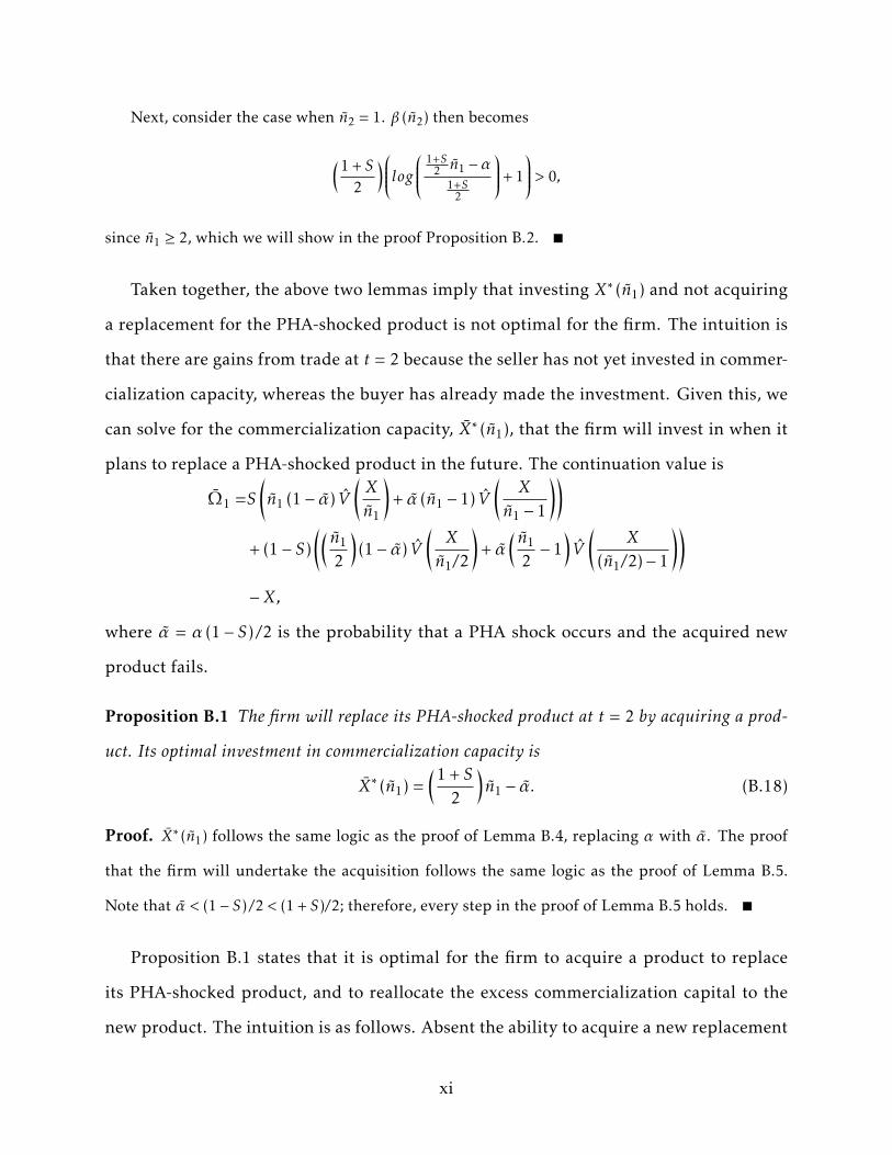
Next, consider the case when n2 = 1. β (n2) then becomes

(1 + S2

)log 1+S2 n1 −α

1+S2

+ 1

> 0,

since n1 ≥ 2, which we will show in the proof Proposition B.2.

Taken together, the above two lemmas imply that investing X∗ (n1) and not acquiring

a replacement for the PHA-shocked product is not optimal for the firm. The intuition is

that there are gains from trade at t = 2 because the seller has not yet invested in commer-

cialization capacity, whereas the buyer has already made the investment. Given this, we

can solve for the commercialization capacity, X∗ (n1), that the firm will invest in when it

plans to replace a PHA-shocked product in the future. The continuation value is

Ω1 =S(n1 (1− α) V

(Xn1

)+ α (n1 − 1) V

(X

n1 − 1

))+ (1− S)

(( n1

2

)(1− α) V

(Xn1/2

)+ α

( n1

2− 1

)V

(X

(n1/2)− 1

))−X,

where α = α (1− S) /2 is the probability that a PHA shock occurs and the acquired new

product fails.

Proposition B.1 The firm will replace its PHA-shocked product at t = 2 by acquiring a prod-

uct. Its optimal investment in commercialization capacity is

X∗ (n1) =(1 + S

2

)n1 − α. (B.18)

Proof. X∗ (n1) follows the same logic as the proof of Lemma B.4, replacing α with α. The proof

that the firm will undertake the acquisition follows the same logic as the proof of Lemma B.5.

Note that α < (1− S) /2 < (1 + S)/2; therefore, every step in the proof of Lemma B.5 holds.

Proposition B.1 states that it is optimal for the firm to acquire a product to replace

its PHA-shocked product, and to reallocate the excess commercialization capital to the

new product. The intuition is as follows. Absent the ability to acquire a new replacement

xi

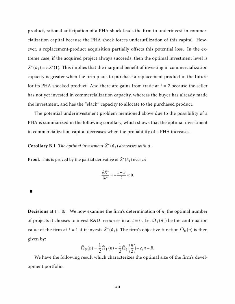
product, rational anticipation of a PHA shock leads the firm to underinvest in commer-

cialization capital because the PHA shock forces underutilization of this capital. How-

ever, a replacement-product acquisition partially offsets this potential loss. In the ex-

treme case, if the acquired project always succeeds, then the optimal investment level is

X∗ (n1) = nX∗(1). This implies that the marginal benefit of investing in commercialization

capacity is greater when the firm plans to purchase a replacement product in the future

for its PHA-shocked product. And there are gains from trade at t = 2 because the seller

has not yet invested in commercialization capacity, whereas the buyer has already made

the investment, and has the “slack” capacity to allocate to the purchased product.

The potential underinvestment problem mentioned above due to the possibility of a

PHA is summarized in the following corollary, which shows that the optimal investment

in commercialization capital decreases when the probability of a PHA increases.

Corollary B.1 The optimal investment X∗ (n1) decreases with α.

Proof. This is proved by the partial derivative of X∗ (n1) over α:

∂X∗

∂α= −1− S

2< 0.

Decisions at t = 0: We now examine the firm’s determination of n, the optimal number

of projects it chooses to invest R&D resources in at t = 0. Let Ω1 (n1) be the continuation

value of the firm at t = 1 if it invests X∗ (n1). The firm’s objective function Ω0 (n) is then

given by:

Ω0 (n) =12Ω1 (n) +

12Ω1

(n2

)− cin−R.

We have the following result which characterizes the optimal size of the firm’s devel-

opment portfolio.

xii

Proposition B.2 There is a unique interior optimal solution, n∗, that maximizes the firm’s

objective function at t = 0. Moreover, n∗ is decreasing in ci in the cross-section.

Proof. It is useful to start by solving for the derivative of Ω∗ (n1). Using the Envelope Theorem,

we have

∂Ω∗1 (n1)∂n1

= S((1− α) V

(X∗ (n1)n1

)+ αV

(X∗ (n1)n1 − 1

)− 1

)+

1− S2

(1− α) V

X∗ (n1)n12

+ αV

X∗ (n1)n12 − 1

− 1

=

1 + S2

(V0 − 1 + log (γ)) + S((1− α) log

(1 + S

2− αn1

)+ αlog

(1 + S

2+

(1 + S) /2− αn1 − 1

))+

1− S2

((1− α) log

(1 + S − α

n1/2

)+ αlog

(1 + S +

1 + S − αn1/2− 1

)).

It is straightforward to verify that the above equation decreases with n1, i.e.

∂2Ω∗1 (n1)

∂n21

< 0,

and (by the last term in ∂Ω∗1 (n1) /∂n1)

limn1→2

∂Ω∗1 (n1)∂n1

= +∞.

To solve for the optimal initial investment n∗, we have

∂Ω∗0 (n∗)∂n∗

=12∂Ω∗1 (n∗)∂n∗

+12

12∂Ω∗1 (n∗/2)∂ (n∗/2)

− ci = 0.

The existence of n∗ follows from the monotonicity of ∂Ω∗1 (n1) /∂n1 and its limit at n1 = 2. The

second statement in the proposition comes from

∂2Ω∗0 (n∗)∂n∗∂ci

=(

12∂2Ω∗1 (n∗)∂n∗2

+12

14∂2Ω∗1 (n∗/2)

∂ (n∗/2)2

)∂n∗

∂ci− 1 = 0.

It is straightforward to verify that∂n∗

∂ci< 0

xiii

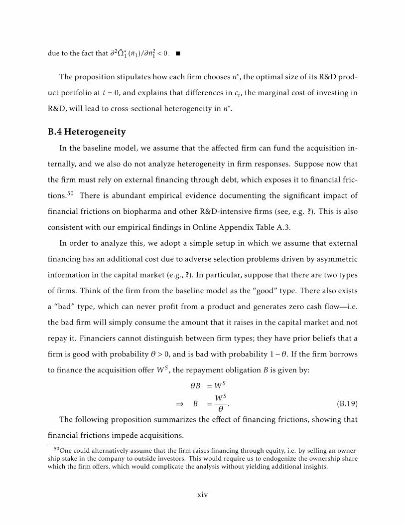
due to the fact that ∂2Ω∗1 (n1) /∂n21 < 0.

The proposition stipulates how each firm chooses n∗, the optimal size of its R&D prod-

uct portfolio at t = 0, and explains that differences in ci , the marginal cost of investing in

R&D, will lead to cross-sectional heterogeneity in n∗.

B.4 Heterogeneity

In the baseline model, we assume that the affected firm can fund the acquisition in-

ternally, and we also do not analyze heterogeneity in firm responses. Suppose now that

the firm must rely on external financing through debt, which exposes it to financial fric-

tions.50 There is abundant empirical evidence documenting the significant impact of

financial frictions on biopharma and other R&D-intensive firms (see, e.g. ?). This is also

consistent with our empirical findings in Online Appendix Table A.3.

In order to analyze this, we adopt a simple setup in which we assume that external

financing has an additional cost due to adverse selection problems driven by asymmetric

information in the capital market (e.g., ?). In particular, suppose that there are two types

of firms. Think of the firm from the baseline model as the “good” type. There also exists

a “bad” type, which can never profit from a product and generates zero cash flow—i.e.

the bad firm will simply consume the amount that it raises in the capital market and not

repay it. Financiers cannot distinguish between firm types; they have prior beliefs that a

firm is good with probability θ > 0, and is bad with probability 1−θ. If the firm borrows

to finance the acquisition offer W S , the repayment obligation B is given by:

θB =W S

⇒ B =W S

θ. (B.19)

The following proposition summarizes the effect of financing frictions, showing that

financial frictions impede acquisitions.

50One could alternatively assume that the firm raises financing through equity, i.e. by selling an owner-ship stake in the company to outside investors. This would require us to endogenize the ownership sharewhich the firm offers, which would complicate the analysis without yielding additional insights.

xiv

Proposition B.3 There exists a θ such that an acquisition is profitable for the firm only if

θ > θ.

Proof. This requires defining a slightly different version of β (j) in equation (B.13), which incor-

porates the repayment obligation:

β(j) =(1 + S

2

)jn1V

(Xjn1

)−(1 + S

2

)(jn1 − 1) V

(X

jn1 − 1

)− W

S

θ.

It is straightforward to see that the above equation increases with θ. By the proof of Proposition

B.1, we know that when θ = 1, β(j) = β(j) > 0. At the same time, β(j) goes to negative infinity as θ

approaches 0. By continuity, there exists θ such that β(j) only if θ > θ.

This proposition states that the magnitude of adverse selection costs will determine

whether the firm will make an acquisition if hit with a PHA shock. That is, if the ini-

tial beliefs of financiers about the firm are too pessimistic, then the (adverse-selection-

induced) external financing cost is too high to make an acquisition profitable.

We now examine how financial frictions interact with firm heterogeneity, and show

that firms with weaker surviving pipelines at t = 2 are more likely to make acquisitions.

In order to do so, in the commercialization stage, let n2 = n1 with probability S ∈ (0,1) and

n2 = jn1 with probability 1 − S and j < 1. Thus, in this setting j is a continuous variable

that represents the strength of the firm’s pipeline, with a lower j representing a poorer

pipeline. Define θ(j) as the cut-off at which an acquisition becomes feasible as a function

of j. Note that a larger θ(j) implies that the cost for doing an acquisition at the threshold

is lower. We now have the following proposition.

Proposition B.4 θ(j) increases with j. In other words, θ is lower for firms with poor product

portfolios than firms with good product portfolios.

Proof. To show this, take the derivative of β(j):

∂β(j)∂j

+∂β(j)∂θ

∂θ(j)∂j

= 0,

xv

or equivalently,W S

θ

∂θ(j)∂j

= −1 + S2

n1log

(1− 1

n1

)> 0.

This implies ∂θ(j)/∂j > 0.

The proposition shows that, holding the magnitude of adverse selection fixed, the firm

has a larger benefit from an acquisition if its product portfolio is weaker. The intuition is

that firms with weaker portfolios have greater excess commercialization capacity that can

be redeployed if they acquire a product in the area from another firm. Hence, they are

more willing to incur the (adverse-selection-induced) external financing cost to do the

acquisition. In contrast, firms with stronger project portfolios have relatively less excess

commercialization capital that can be redeployed to a new project, due to the fact that

their portfolios have more projects and are thus more promising. These firms therefore

have weaker incentives to pursue an acquisition, and are not willing to bear an external

financing cost in order to do so.

B.5 Discussion: Extensions

In this section, we discuss how our analysis would be affected by other possible ex-

tensions related to projects choices, introducing competitors, and assumptions related to

incomplete contracting.

Internal Initiation

The baseline model assumes that the firm can only acquire a project to replace an affected

product after the PHA shock. We now discuss the possibility of alternative actions: in-

ternally developing a new replacement product either in the same area or in a different

area. Developing a product in a new area incurs costs of both R (in the area) and ci (in

the product). If R is large enough, then it will not be worthwhile to expend it on one

replacement product. Furthermore, downstream assets may be area-specific, and thus

cannot be redeployed to a project in a new area. Therefore, developing such a project will

xvi

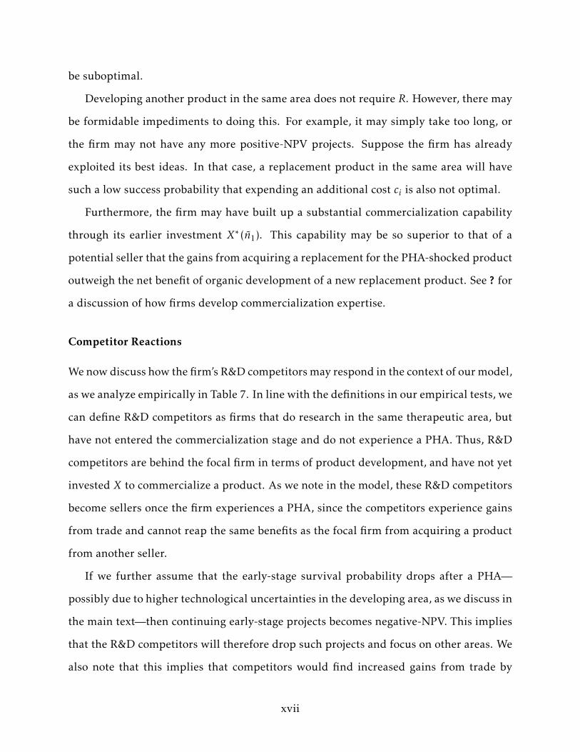
be suboptimal.

Developing another product in the same area does not require R. However, there may

be formidable impediments to doing this. For example, it may simply take too long, or

the firm may not have any more positive-NPV projects. Suppose the firm has already

exploited its best ideas. In that case, a replacement product in the same area will have

such a low success probability that expending an additional cost ci is also not optimal.

Furthermore, the firm may have built up a substantial commercialization capability

through its earlier investment X∗ (n1). This capability may be so superior to that of a

potential seller that the gains from acquiring a replacement for the PHA-shocked product

outweigh the net benefit of organic development of a new replacement product. See ? for

a discussion of how firms develop commercialization expertise.

Competitor Reactions

We now discuss how the firm’s R&D competitors may respond in the context of our model,

as we analyze empirically in Table 7. In line with the definitions in our empirical tests, we

can define R&D competitors as firms that do research in the same therapeutic area, but

have not entered the commercialization stage and do not experience a PHA. Thus, R&D

competitors are behind the focal firm in terms of product development, and have not yet

invested X to commercialize a product. As we note in the model, these R&D competitors

become sellers once the firm experiences a PHA, since the competitors experience gains

from trade and cannot reap the same benefits as the focal firm from acquiring a product

from another seller.

If we further assume that the early-stage survival probability drops after a PHA—

possibly due to higher technological uncertainties in the developing area, as we discuss in

the main text—then continuing early-stage projects becomes negative-NPV. This implies

that the R&D competitors will therefore drop such projects and focus on other areas. We

also note that this implies that competitors would find increased gains from trade by

xvii

selling these projects to the firms experiencing PHA shocks, thus strengthening our main

results.

Incomplete Contracting and the Acquisition Choice

A question that arises is why the PHA-shocked firm would acquire a replacement product

from another firm rather than selling its excess commercialization capacity. A potential

explanation is incomplete contracting.

To see this, assume that the firm’s commercialization investment consists of a fixed,

observable investmentX, which we have modeled, plus an unobservable, non-contractable

variable investment per product of y in continued support for its downstream commer-

cialization capacity. Also assume that the marginal cost of this investment is lower for

the firm that initially established this commercialization capacity (the PHA firm) than

for others. Then the incomplete contracting theory of ? and ? indicates that the efficient

arrangement will be for the PHA-shocked firm to acquire the replacement product from

another firm, rather than to sell its excess commercialization capacity to that firm. See

also ?.

The reason is that a sale of excess commercialization capacity by the PHA-shocked

firm will result in the selling firm undersupplying y for continued support for its down-

stream commercialization assets. Incomplete contracting theory says that a solution to

this problem is to give residual ownership of the asset to the party whose undersupply of

productive inputs has a bigger impact on the output. In this setting, it is the PHA-shocked

firm with the excess downstream commercialization capacity.

xviii