Finding “Anomalies” in an Arbitrary Image · Finding “Anomalies” in an Arbitrary Image ... the filters are statistically as independent as possible. ... valuable for process

Finding “Anomalies” in an Arbitrary Image

Toshifumi Honda Shree K. Nayar Hitachi Ltd. Columbia University

Production Engineering Research Laboratory Department of Computer Science 292 Totsuka, Yokohama 244-08 17, Japan

[email protected]

Abstract

A fast and general method to extract “anomalies ’’ in an arbitrary iniage is proposed. The basic idea is to compute a probability density f o r sub-regions in an image, conditioned upon the areas surrounding the sub-regions. Lin- ear estimation and Independent Component Analysis ( ICA) are combined to obtain the probability estimates. Pseudo non-parametric correlation is used to group sets of similar surrounding patterns, from which a probability f o r the occurrence of a given sub-region is derived. A carefully de- signed multi-dimensional histogram, based on compressed vector representations, enables eficient and high-resolution extraction of anonlalies from the image. Our current (un- optimized) implementation performs anomaly extraction in about 30 seconds f o r a 640x480 image using a 700 M H z PC. Experimental results are included that demonstrate the perforniance of the proposed method.

1 What is an Image “Anomaly”?

Humans have a knack for quickly finding portions of a scene that are in some sense anomalous. This is true even when the scene is complex and includes multiple patterns or textures. Consider the examples shown in Figure 1. The coffee stain on the table cloth and the squirrel perched in the hole in the brick wall very quickly draw our attention. We refer to such “unusual” or “unexpected” portions of an image as anomalies. One might consider segmenting the image and analyzing each segmented portion to infer anomalies. However, automatic segmentation of complex scenes remains an open problem and cannot be relied upon as a general solution to anomaly extraction. In short, the problem is a hard one from the perspective of computer vision.

This paper proposes a fast and general technique for extracting anomalies in images. It should be mentioned that anomaly detection can be approached in two ways. The first is contextual, where an anomaly is an unexpected event,

New York, NY 10027 nay ar @ cs .columbi a.edu

(a) (b) Figure 1. Some examples of image anomalies (within cir- cles). (a) A coffee stain on a tablecloth. (b) A squirrel in a hole in a brick wall.

given the high-level context of the scene. This is very hard perceptual problem and is not the goal of our work. The second approach, which is the one we take, operates at a lower level by looking for unexpected local patterns in an image. This too is a challenging problem. For instance, in our tablecloth example in Figure 1, one sees different textures at different scales of resolution. Some of the patches (texels) appear frequently while others do not. Therefore, we cannot define anomalies as merely image patterns that occur rarely and hence have low probability. Instead, we characterize “anomalies” using conditional probability densities. A region that is “normal” can be expected from its neighbohood, or is highly probable given its surrounding. In contrast, an area that is “abnormal” has little in common with its neighbohood, and its likelihood, conditioned on its neighborhood, should be relatively small.

Related work on texture synthesis and recognition has used joint probability distributions of local image frequency measures. The specific representations used include steerable pyramids [71, textons [ 101, and multi-resolution histograms [l]. These representations, however, are not appro- priate for anomaly detection. This is because the anomalies themselves serve to corrupt the representations used to recognize them. Another drawback is that these representations cannot adequately capture the joint probability distribution of an image region based on a neighborhood that has high frequencies (see 151 for supporting arguments).

5 16 0-7695-1143-0/01 $10.00 0 2001 IEEE

mailto:[email protected]

Manduchi and Portilla [ I 11 proposed a novel representation based on Independent Component Analysis (ICA) for texture synthesis and clustering. The local texture is represented as a set of filter responses, each filter being a linear combination of steerable filters. ICA is used to ensure that the filters are statistically as independent as possible. This representation makes the calculation of region probabilities simple, but it shares the problems inherent to all frequency- based joint distributions; the lower frequencies may be influenced by portions of the image we seek to extract.

Finally, Efros and Leung [51 proposed a texture synthesis method that computes the probability of a pixel value based on its surrounding. Their algorithm calculates a conditional probability to synthesize new pixels. This is done by finding areas in a sample texture that are similar to the area around the pixel to be synthesized. This approach works well but its computational cost is great, making it too slow for many real-world applications. Moreover, it is not suitable for our task as anomalies generally include more than a single pixel and have arbitrary shapes.

Here, we propose a method that detects anomalies in an arbitrary image. We calculate the probability of a region’s occurrence, conditioned on its neighborhood. Several tech- niques and representations are used make the algorithm efficient and robust. These include ICA for representing local regions, non-parametric correlation to suppress the effects of anomalies on our representations, the Discrete Co- sine transform (DCT) and the Karhunen-Loeve transform (KLT) to represent neighborhoods, and multi-dimensional histograms for classification. The current implementation of our algorithm extracts anomalies from a 640x480 image in about 30 seconds using a 700 MHz PC. Several experimental results are included that show the performance of our method.

Anomaly detection is a problem with wide implications. In an inspection task, it provides a powerful means to “flag” visual defects without prior knowledge. This information is valuable for process control. In the context of image editing, a user can input an image or a part of it, and have the algorithm find anomalies. The anomalies can then be re- moved from the image and their areas filled using texture synthesis based on data available in the rest of the image.

’

2 Representation of Patterns

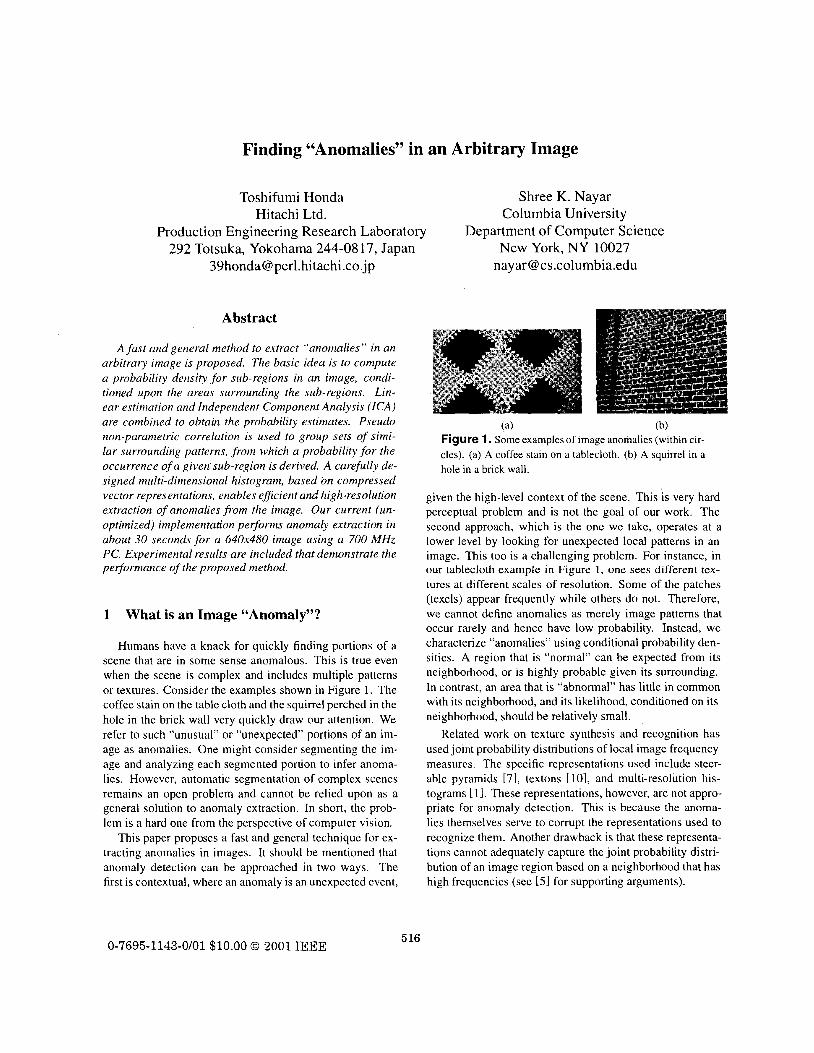
Consider an arbitrary image I consisting of various patterns. Each small region (sub-region) in the image bears a relationship to its immediate neighborhood. We begin by defining what we mean by sub-regions and their neighborhoods (see Figure 2). A vector composed of the brightness values within a sub-region centered at a point x is denoted by the “evaluation vector” e(.) = (el(z), e2(z) ... eN(z)) . The vector representation of the surrounding brightness Val-

Figure 2. For a point 5 , the subregion and its neighborhood are represented by the evaluation vector e(.) and the conditional vector w ( z ) , respectively.

ues is called the “conditional vector” and is denoted by U(.) = (w1(x),wg(z) ... w ~ ( 2 ) ) . The conditional probability of e(z)is denoted by P(e(z)Jw(z) ) . This probability can be calculated from the following set:

E ( z ) = {e(z’) : r (w(z ’ ) ,w( z ) ) < A w n d - z > E } (1)

where, r (w(z ’ ) ,w( z ) ) is a measure of similarity between neighborhood patterns w(z ’ ) and w(z) , and Aw is a similarity threshold. The constraint that z’-z must be larger than L

helps us prevent anomalies from influencing the calculation of the probability distribution too much. We will ideally be well outside the boundaries of any potential anomaly when making our comparisons.

2.1 Computing the Conditional Probability

There are a few important issues that face us when evaluating P(e(x)lw(z)):

Low density of the feature space: This problem is due to the fact that the feature space spanned by ( e T , wT)T is huge relative to the number of evaluation and conditional vectors available in a given image.

Inaccuracies in the similarity between conditional vectors: This problem stems from the fact that, because the conditional vectors are large, they are easily con- taminated by portions of anomalies. Anomalies often contain points that are distant in their values from points in non-anomalous regions. This easily ham- pers vector comparison measures such as the sum-of- squared-distances (SSD).

Large numbers of comparisons: Note that, to compute the joint distribution, we need to find all conditional vectors that resemble w, for each point z in the image. Further, the larger the evaluation vector, the larger the conditional vector, and hence greater the resulting computational cost.

To ameliorate these difficulties, we explore new representations for both evaluation and conditional vectors. Problems 1 and 2 will be addressed in section 2.2. Prob- lem 3 will be addressed in section 2.3.

517

2.2 Representing Evaluation Vectors Accurate calculation of the probability density

P ( e ( z ) l w ( z ) ) over all ( eT , wTlT is usually impossi- ble because the number of sample points we have available to us is small compared to dimensionality of the feature space. To alleviate this problem, we use Independent Component Analysis (ICA) and linear estimation.

In general, ICA calculates a set of bases that are as mutually independent as possible. Consider a random set of variables {yl, y2 ...yn}. If these variables are mutually independent, their joint probability density can be factorized

denotes the probability density of yz . Here, more accurate estimation of P ( y z ) is usually possible because the feature space spanned by yz is one-dimensional. The reduction in dimensionality increases the density of sample points and makes the estimation of the joint probability distribution faster and more accurate.

Using ICA, we seek to transform each evaluation vector e into the vector y = (y1, y2 . . . y ~ ) , such that the elements of y are as mutually independent as possible. Here, K is the number of terms that result from ICA decomposition. Then, the conditional probability we seek to calculate can be written as:

If we could transform y such that it is independent of w , the above expression can be greatly simplified; the conditional probability P(y, lw) can be calculated from just the probability function P( yz). Unfortunately, complete independence between each y and w cannot be expected. However, the degree of independence can be increased significantly if we decorrelate y and w to reduce the sensitivity of P ( y z ( w ) to changes in w.

To this end, before transforming e using ICA, the correlated component between e and w is subtracted from e. This decorrelation of the evaluation sub-region e from the surrounding pattern w helps us find independent components for the sub-region that are not greatly influenced by its surroundings. The desired decorrelation is achieved by computing the estimation matrix A that minimizes:

(3)

If e consists of a large number of pixels (and it usually does), the estimation of A may be expensive. One can obtain an approximate solution by using just a single element of e, namely e,(z), that corresponds to the center pixel c of the evaluation sub-region. Thus, expression (3) becomes

(4)

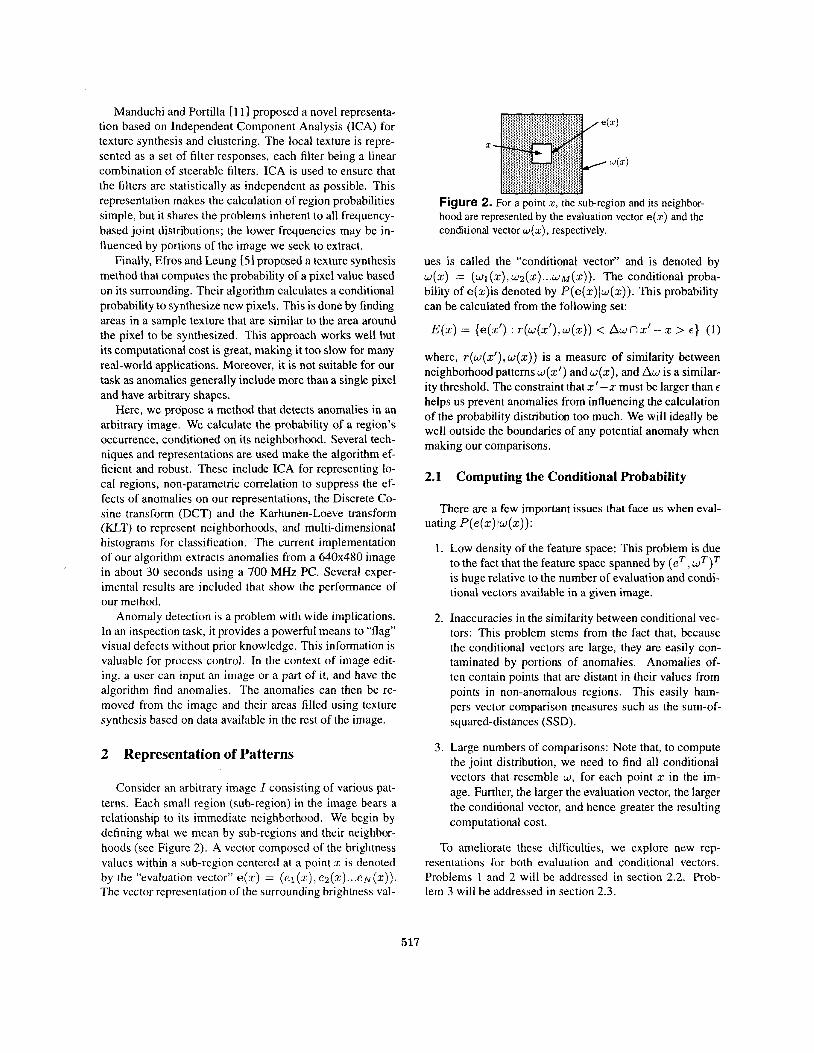
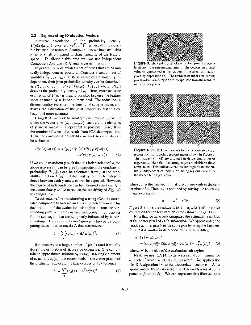
Figure 3. Thc center pixel 01 each subregion IS decorrelated from the surrounding region. The decorrelated pixel value is represented as the residue of the linear estimation given by expression (5). The residues of other (off-center) pixels within a sub-region are interpolated from the residues of the center pixels.

Figure 4. The ICA components for the decorrelated (sub- region from surrounding region) image shown in Figure 3 . The images (a) - (d) are arranged in descending order of negentropy. Note that the strong edges are visible in these components. This indicates that the sub-regions are not en- tirely independent of their surrounding regions even after the decorrelation procedure.

where, a, is the row vector of A that corresponds to the center pixel of e . Then, a, is obtained by solving the following linear expression:

-_ a ,=wwT (5 )

Figure 3 shows the residue e,(z’) - aTw(z ’ ) of the above estimation for the textured tablecloth shown in Fig. 1 (a).

Note that we have only computed the estimation residues at the center pixel of each sub-region. We approximate the residue at other pixels in the subregion by using the Lanczos filter that is similar in its properties to the Sinc filter:

exf(z) - a z , w ( z )

= Sinc(g)Sinc(%)(e , (z ’ ) - aTw(z’)) (6 )

where, N is the size of the evaluation sub-region. Next, we use ICA [41 to derive a set of components for

e, each of which is ideally independent. We applied the FastICA algorithm [81 to the decorrelated vector e - A T w approximated by equation (6). FastICA yields a set of components (filters) {fi}. We can represent this filter set as a

518

matrix F = (fi, f ~ . . . f ~ ) ~ . The ICA dimension K is less than the number of pixels in the sub-region because components which represent low energy terms of the decomposition are eliminated. The filter responses for any sub-region in our image, y = FT(e - A T w ) , serves as our chosen representation for the region’. FastICA computes the basis iteratively to find the bases. Its convergence, however, is usually fast. 2.3 Representing Conditional Vectors

Unfortunately, an ICA decomposed evaluation vector will generally not be completely independent of its surrounding pattern, even after the decorrelation process (see Figure 3). Therefore, the joint distribution of is still required in order to evaluate equation (2). This calculation demands that we find every vector similar to ( ~ ~ ( z ) ~ , ~ ( z ) ~ ) ~ in the image. And, as we discussed, we must be very careful not to allow portions of an “anomaly” to influence any comparisons between vectors that we may make. We take the idea of nonparametric correlation to reduce the influence of anomalies. This step is described in section 2.3.1.

As noted before, another problem faced in calculating P(e (x ) lu ( z ) ) is that the size of w can be very large. If we assume the size of the evaluation vector to be 32 x 32, the size of ~ ( x ) may be more than 150 x 150. The identification of all the conditional vectors that resemble w ( z ) cannot be done in reasonable time if w is so large. To make this process efficient we compress the conditional vector w. This process is outlined in section 2.3.2. 2.3.1 Similarity Using Non-Parametric Correlation

A good way to suppress the influence of anomalies is to use a non-parametric correlation technique, such as Spear- man’s rank-order correlation [91. However, applying Spear- man’s method to our problem proves difficult, as it requires us to assign ranks to every element of the conditional vector under consideration, which is computationally intensive. Therefore, instead of assigning ranks, we histogram equal- ize the whole image. The equalized pixel value in a vector is then taken as the rank of that pixel in our computations. The advantage of histogram equalization for reduction of anomaly influence is shown in Fig. 5.

We denote the vector representation of the conditional vector in the histogram equalized image as w’ = ( ~ & , w ; . . . w h ) ~ , where, the w: correspond to the ranks of the corresponding pixel values in the image. The measure based on pseudo non-parametric correlation that is used to

’ FatICA yields a set of components such that the coefficients y are distributed with minimal gaussianity. The lack of gaussianity is measured by negentropy of y,, J(y,) . Direct calculation of negentropy is difficult, so an approximation is frequently used. We use one of the classical ap- proximations, which makes use of higher-order moments. This enables high-sped calculation.

(a) Original image (b) Equalized image

Figure 5. The original image (a) is histogram equalized to get image (b). After equalization, the bright flower has less influence on the similarity measure used to compare surrounding pattems w. The number of bins used for equalization is determined such that pixel values of the equalized image have the same variances as in original image.

find the similarity between conditional vectors is defined as:

This measure draws from both parametric linear correlation and non-parametric correlation.

2.3.2

A good way to compactly represent our conditional vectors is by using the Karhunen-Loeve transform (KLT). However, the problem with IUT is that it is computationally costly because of the dimensionality of w.’Most of the cost is in- volved in the computation of the covariance matrix needed in KLT. For instance, the covariance matrix size would be about 22K x 22K for a conditional vector size of 150x 150.

As noted by Hamidi and Pearl [61, KLT coefficients can be approximated by DCT coefficients for signals that can be modeled by one-dimensional Markov Random Fields. Hence, we use a two-step compression process; DCT fol- lowed by KLT. That is, w’(z) is transposed into DCT space to reduce its redundancy and then the KLT is applied. No- tice that w ’ ( ~ ) has to be calculated for every z and it has a hole at its center which corresponds to the evaluation sub- region e. A large DCT block does not greatly improve the compression rate, therefore, ~ ’ ( z ) is divided into several small blocks (8x8 or 16x 16, in our experiments) so as to efficiently calculate DCT the coefficients. The use of blocks is illustrated in Fig. 6.

The farther blocks from z are more influenced by the topological variations in the rest of image than closer blocks. This influence is particularly strong in the case of high frequencies. Therefore, we need to suppress the con- tribution of high-frequency components for blocks that are farther away from Z. This suppression is proportional to the

Efficient Compression of Conditional Vectors

519

distance from x. We also note that the blocks that are farther away from x are less relevant than block close to the evaluation vector. To account for these effects, we introduce a diagonal matrix G(d) whose elements are weights associ- ated with individual blocks, each weight being a function of the distance d of the block from x. One last thing we need to account for is the normalization that is contained in equation(7). More formally, let b, be the DCT representation of the ith block of w‘, and c be our weighted DCT representation of w’. Then:

’ (8) (brG(d0); bTG(d1). . .bzG(dm))T Ilb;fG(do), bTG ( d i ) . . .bT,G(&) I1

c =

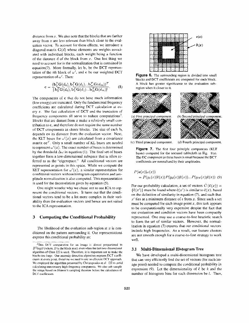
Figure 6. The surrounding region is divided into small blocks and DCT coefficients are computed for each block. A block has greater significance to the evaluation sub- region when i t closer to it.

The components of c that do not have much information ( low energy) arc truncated. Only the fundamental frequency coctlicicntj arc calculated Juring DCT calculation at every r The I h \ t calculation 01 DCT and the truncation of frequency components all serve to reduce computations2. (a) First principal component. (b) Second principal component. Block\ thiit arc di4tant from .I mahc a rclativdy small con- tribution to c , and therclorc do not require the u m c number of DCT component4 a\ clowr bloch4 The w e ol each b, depcndz on its distance from the evaluation vcctor Next, the KLT barn for r L . ~ ’ ( ~ j arc‘ crtlculatcd from a covari:incc

\ I

matrix ccT. Only a small number of KL bases are needed to represent ~ ’ ( I c ) . The exact number of bases is determined by the threshold A w in equation ( I ) . The final set of bases together form a low-dimensional subspace that is often re- ferred to as the “eigenspace.” All conditional vectors are represented as points in this space. While we compute the KLT representation for U’(.), a similar representation for conditional vectors without histogram equalization and am- plitude normalization is also computed. This representation

(c) Third principal component. (d) Fourth principal component.

Figure 7. The first four principle components (KLT bases) computed for the textured tablecloth in Fig. l(a). The DC component in these bases is small because the DCT coefficients are normalized by their amplitudes.

P(e(z)lw(x)) = P(Yl (x)1e(5))P(Y2(x)(e(x))...P(YN(IC)(e(x)) (9)

is used for the decorrelation given by equation (5). One might wonder why we chose not to use ICA to rep-

resent the conditional vectors. It turns out that the conditional vectors tend to be a lot more complex in their vari- ability than the evaluation vectors and hence are not suited to the ICA representation.

For our probability calculation, a set of vectors d (E(x)) = {C(x’)} must be found where C(x’) is similar to C(z), based on the definition of similarity in equation (7), and such that x’ lies at a minimum distance of E from x. Since such a set must be computed for each image point x, this task appears to be computationally very expensive despite the fact that

3 Computing the Conditional Probability

The likelihood of the evaluation sub-region at IC is conditioned on the pattern surrounding it. Our representations express this conditional probability as:

’This DCT computation for an image is almost proportional to B210gB (where. B is the block size), even when the fast two-dimensional algorithm of Chan [21 is used. Therefore, it is important not to make the blocks too large. Our anomaly detection algorithm requires DCT coefficients at every point, therefore we need to use an efficient DCT approach. We employed the algorithm presented by Christopoulos et al. U31 to avoid calculating unnecessary high-frequency components. We also sub-sample the image based on Shanon’s sampling theorem before the calculation of DCT coefficients.

our evaluation and condition vectors have been compactly represented. One may use a coarse-to-fine heuristic search to form the set of similar vectors. However, the normalization in equation (7) ensures that our conditional vectors include high frequencies. As a result, our feature clusters are not smooth enough for a coarse-to-fine strategy to work well.

3.1 Multi-Dimensional Histogram Tree We have developed a multi-dimensional histogram tree

that can very efficiently find the set of vectors (for each image point) needed to compute the conditional probability in expression (9). Let the dimensionality of E be k and the number of histogram bins for each dimension be 1. Then,

520

Index Table

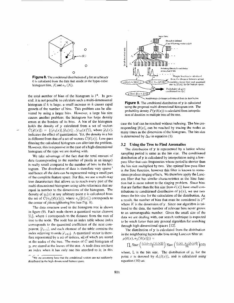
0 Figure 8. The conditional distribution of y for an arbitrary e is calculated from the data that reside in the hyper-cubic histogram bins, [e] andn, ([e]).

the total number of bins of the histogram is 1 ‘. In general, it is not possible to calculate such a multi-dimensional histogram if IC is large; a small increase in k causes rapid growth of the number of bins. This problem can be alle- viated by using a larger bins. However, a large bin size causes another problem; the histogram has large density errors at the borders of its bins. A bin of the histogram holds the density of y calculated from a set of vectors

indicates the effect of quantization. Yet, ;he density in a bin is different from that of a set of vectors C(E(x)) . Low-pass filtering the calculated histogram can alleviate the problem. However, this is expensive in the case of a high-dimensional histogram of the type we are dealing with.

We take advantage of the fact that the total amount of data (corresponding to the number of pixels in an image) is really small compared to the number of bins in the histogram. The distribution of data is therefore very sparse3 and hence all the data can be represented using a small part of the complete feature space. For this, we use a multi-way tree datastructure that allows us to reach every part of the multi-dimensional histogram using table references that are equal in number to the dimensions of the histogram. The density of yz(z) at any arbitrary point z is calculated from the set of C(n,([E(z)])) , where n,([e(lc)]) corresponds to the center of j t h neighboring bin (see Fig. 8).

The data structure used in the histogram tree is shown in figure (9). Each node shows a quantized vector element [&I, where i corresponds to the distance from the root of tree to the node. The node has an index table whose index corresponds to the quantized coefficient of the next component, [tZ+1], and each element of the table contains the index referring to node [C,,,]. A quantized vector is therefore represented by a set of indices, all Of which are stored at the nodes of the tree. The mean of C and histogram of yL are stored at the leaves of the tree. A node does not have an index when i t has only one bin attached to it; in this

e q[E(.) l> = { ( [ h ( x ) ] , [ W ) ] . . . [ ~ A 4 ( 4 1 ) } > where [&(x)l

We are assuming here that the conditional vectors are not uniformly distributed in the high-dimensional feature space.

Branch IS deleted if no following vector exists

Probability Density for each lattice at every leaf of tree

c

froiii the distance between actual

I) Probability of U:(.) conditioned on c(.z)

Neighboring suh-image is eliminated from the disuihulion

Figure 9. The conditional distribution of y is calculated using the proposed multi-dimensional histogram tree. The probability density P(yle(z ) ) is calculated from interpolation of densities in multiple bins of the tree.

case the leaf can be reached without indexing. The bin corresponding [e(x)] can be reached by tracing the nodes as many times as the dimension of the histogram. The bin size is determined by ALLI in equation ( I ) .

3.2 Using the Tree to Find Anomalies The distribution of y is represented by a lattice whose

sampling period is same as the bin size. The conditioned distribution of y is calculated by interpolation using a low- pass filter that cuts frequencies whose period is shorter than the bin size multiplied by two. The optimal low-pass filter is the Sinc function, however this filter is known to some- times produce ringing effects. We therefore apply the Lanc- zos filter that has similar characteristics as the Sinc function but is more robust to the ringing problem. Since bins that are farther than the bin size from E(.)) have small contributions to conditioned distribution of y ( ~ ) , we use two times the bin size for the calculation of the distribution. As a result, the number of bins that must be considered is 2 K where K is the dimension of y . Since our algorithm is tai- lored to the data, the number of relevant bins never grows to an unmanageable number. Given the small size of the data we are dealing with, our search technique is expected to be much faster than any general algorithm for searching through high-dimensional spaces [121.

The distribution of y is calculated from the distribution in the neighboring hypercube bins using Lanczos filter as: /.(C(X), % ( P ( X ) l ) ) = n, Sinc ( E r (.)-nt(liv ‘“’I)) Sinc (e7 (+;;I1S7 (s)l)

where, L is the bin size. The distribution of yz for the point z is denoted by dZ(i.(z)), and is calculated using equation (10) as:

52 1

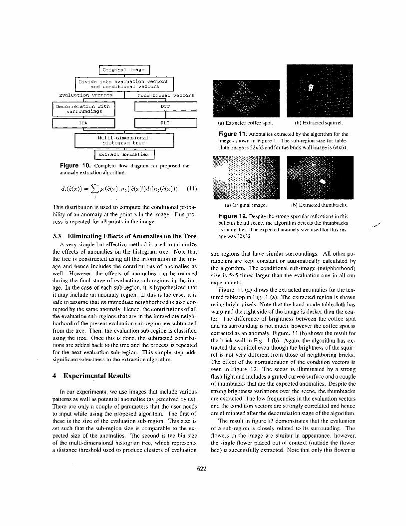
I Original Image I Divide into evaluation vectors

and conditional vectors

Evaluation vectors I Conditional vectors I 1

Decorrelation with DCT surroundings 1

I I ICA KLT 1

Figure 10. Complete flow diagram for proposed the anomaly extraction algorithm.

This distribution is used to compute the conditional probability of an anomaly at the point 2 in the image. This process is repeated for all points in the image.

3.3 Eliminating Effects of Anomalies on the Tree A very simple but effective method is used to minimize

the effects of anomalies on the histogram tree. Note that the tree is constructed using all the information in the image and hence includes the contributions of anomalies as well. However, the 'effects of anomalies can be reduced during the final stage of evaluating sub-regions in the image. In the case of each sub-region, it is hypothesized that it may include an anomaly region. If this is the case, it is safe to assume that its immediate neighborhood is also cor- rupted by the same anomaly. Hence, the contributions of all the evaluation sub-regions that are in the immediate neighborhood of the present evaluation sub-region are subtracted from the tree. Then, the evaluation sub-region is classified using the tree. Once this is done, the subtracted contributions are added back to the tree and the process is repeated for the next evaluation sub-region. This simple step adds significant robustness to the extraction algorithm.

4 Experimental Results

In our experiments, we use images that include various patterns as well as potential anomalies (as perceived by us). There are only a couple of parameters that the user needs to input while using the proposed algorithm. The first of these is the size of the evaluation sub-region. This size is set such that the sub-region size is comparable to the expected size of the anomalies. The second is the bin size of the multi-dimensional histogram tree, which represents a distance threshold used to produce clusters of evaluation

(a) Extracted coffee spot. (b) Extracted squirrel.

Figure 11. Anomalies extracted by the algorithm for the images shown in Figure 1. The sub-region size for tablecloth image is 32x32 and for the brick wall image is 64x64.

(a) Original image. (h) Extracted thurribtacks

Figure 12. Despite the strong specular reflections in this bulletin board scene, the algorithm detects the thumbtacks as anomalies. The expected anomaly size used for this image was 32x32.

.A'

sub-regions that have similar surroundings. All other parameters are kept constant or automatically calculated by the algorithm. The conditional sub-image (neighborhood) size is 5x5 times larger than the evaluation one in all our experiments.

Figure. 11 (a) shows the extracted anomalies for the textured tabletop in Fig. 1 (a). The extracted region is shown using bright pixels. Note that the hand-made tablecloth has warp and the right side of the image is darker than the center. The difference of brightness between the coffee spot and its surrounding is not much, however the coffee spot is extracted as an anomaly. Figure. 11 (b) shows the result for the brick wall in Fig. 1 (b). Again, the algorithm has extracted the squirrel even though the brightness of the squirrel is not very different from those of neighboring bricks. The effect of the normalization of the condition vectors is seen in Figure. 12. The scene is illuminated by a strong flash light and includes a grated curved surface and a couple of thumbtacks that are the expected anomalies. Despite the strong brightness variations over the scene, the thumbtacks are extracted. The low frequencies in the evaluation vectors and the condition vectors are strongly correlated and hence are eliminated after the decorrelation stage of the algorithm.

The result in figure 13 demonstrates that the evaluation of a sub-region is closely related to its surrounding. The flowers in the image are similar in appearance, however, the single flower placed out of context (outside the flower bed) is successfully extracted. Note that only this flower is

522

(a) Original image. (b) Extracted flower.

Figure 13. The image in (a) includes several flowers that are similar in appearance. However, only the Rower that is outside the Rower bed is extracted as an anomaly (see (b)).

extracted as an anomaly. Finally, Table. 1 shows the computational time required

for each part of our algorithm. Note that on average the algorithm takes about 30 seconds to process a 640x480 image using a 700 MHz PC. It is worth mentioning that the current implementation of the algorithm is not optimized.

5 Conclusion

We have proposed a general method for extracting anomalies from an arbitrary image. By using the probability density for sub-regions in an image conditioned upon their surrounding, the developed algorithm can recognize irregular parts of a complex image. The algorithm em- ploys linear estimation, Independent Component Analysis (ICA) and Karhunen Lokve Transform (IUT) for quick and compact representation of image data. A carefully de- signed multi-dimensional histogram tree enables efficient and high-resolution extraction of anomalies from the image. The proposed algorithm has potential uses in a variety of application domains, ranging from unsupervised visual inspection to interactive image editing.

6 Acknowledgements

This research was conducted at the Department of Com- puter Science, Columbia University. We would like to thank Dr. Yasuo Nakagawa at Hitachi Ltd for his encouragement to this research.

References

[ I ] J. S . De Bonet. Multiresolution sampling procedure for analysis and synthesis of texture images. Proceedings of ACM

Table 1. Computational time taken by the components of the anomaly detection algorithm on a 700 MHz PC.

SIGRAPH, 1997.

S.C. Chan and K.L. Ho. A new two-dimensional fast cosine transform algorithm. IEEE Trans. on Signal Processing., 39, 1991.

C.A. Christopoulos, J . Bormans, A.N. Skodras, and J. Cor- nelis. Efficient computation of the two-dimensional fast cosine transform. In Proc. SPIE2238. 1994.

P. Common. Independent component analysis: A new con- cept? Signal Processing, 36(3):287-3 14, 1994.

A.A. Efros and T. K. Leung. Texture synthesis by non- parametric sampling. Proceedings of the 7th International Conference on Computer Vision, 1999.

M. Hamidi and J. Pearl. fourier transforms of markov-1 signals. Acoustic Speech Signal Proc., ASSP-24, 1976.

Comparison of the cosine and IEEE Trans. of

D. Heeger and J . Bergen. sislsynthesis. Proceedings of ACM SIGRAPH, 1995.

Pyramid-based texture analy-

A. Hyvarinen. Fast and robust fixed-point algorithms for independent component analysis. lEEE Transactions on Neu- ral Networks, 10(3):626-634, 1999.

E.L. Lehmann. Nonparanietrics:Statistical Methods Bused on Ranks. Holden-day, 1975.

[ I O ] J. Malik, S. Belongie, J . Shi, andT. Leung. Textons, contours and regions: Cue integration in image segmentation. Pro- ceedings of the 7th International Conference on Computer Vision, 1999.

[ I 11 R. Manduchi and J. Portilla. Independent component analysis of textures. Proceedings of the 7th International Confer- ence on Computer Vision, 1999.

[I21 S. Nene and S. Nayar. A simple algorithm for nearest neighbor search in high dimensions. IEEE Transuctions on Puttern Analysis & Machine Intelligence, 19:989-1003, 1997.

523

Documents

Finding “Anomalies” in an Arbitrary Image · Finding “Anomalies” in an Arbitrary Image ... the filters are statistically as independent as possible. ... valuable for process