faculty of science and engineering

mathematics and applied mathematics

Finding best minimax approximations with the Remez algorithm

Bachelor’s Project Mathematics

October 2017

Student: E.D. de Groot

First supervisor: Dr. A.E. Sterk

Second assessor: Prof. Dr. H.L. Trentelman

Abstract

The Remez algorithm is an iterative procedure which can be used tofind best polynomial approximations in the minimax sense. We presentand explain relevant theory on minimax approximation. After doing so,we state the Remez algorithm and give several examples created by ourMatlab implementation of the algorithm. We conclude by presenting aconvergence proof.

2

Contents

1 Introduction 4

2 Convexity 72.1 Definitions . . . . . . . . . . . . . . . . . . . . . . . . . . . . . . . 72.2 Results . . . . . . . . . . . . . . . . . . . . . . . . . . . . . . . . . 8

3 Characterization of the best polynomial approximation 10

4 The alternation theorem 124.1 The Haar condition . . . . . . . . . . . . . . . . . . . . . . . . . . 124.2 The alternation theorem . . . . . . . . . . . . . . . . . . . . . . . 154.3 An applicable corollary . . . . . . . . . . . . . . . . . . . . . . . . 17

5 The Remez algorithm 185.1 Two observations . . . . . . . . . . . . . . . . . . . . . . . . . . . 185.2 Statement of the Remez algorithm . . . . . . . . . . . . . . . . . 195.3 A visualization of the reference adjustment . . . . . . . . . . . . 20

6 Testing our implementation of the Remez algorithm 226.1 Comments about the implementation . . . . . . . . . . . . . . . . 226.2 Examples . . . . . . . . . . . . . . . . . . . . . . . . . . . . . . . 236.3 Conclusion . . . . . . . . . . . . . . . . . . . . . . . . . . . . . . 31

7 Proof of convergence of the Remez algorithm 327.1 Theorem of de La Vallee Poussin and the strong unicity theorem 327.2 Proof of convergence . . . . . . . . . . . . . . . . . . . . . . . . . 357.3 Completing the argument . . . . . . . . . . . . . . . . . . . . . . 38

8 Conclusion 41

A Technical detail 42

B Adjustment of the reference 42

C Matlab codes 44

References 49

3

1 Introduction

Roughly speaking, approximation theory is a branch of mathematics which dealswith the problem of approximating a given function by some simpler class offunctions. The general formulation of the best approximation problem can begiven as follows. Given a subset Y of a normed linear space X and an elementx ∈ X, can we find an element y∗ ∈ Y that is closest to x? That is, can we finda y∗ ∈ Y so that

||x− y∗|| ≤ ||x− y||for all y ∈ Y ? Several questions can be asked.

• Under what conditions on Y does a best approximation exist?

• If it exists, is it unique?

• If it exists, how can we find it?

• What happens if we choose a different norm?

Answers to the questions formulated above can be found in standard books onapproximation theory, such as [1] or the classical book by Cheney [2]. Anotheroverview of different topics in approximation theory can be found in [3].

In some cases, the best approximation problem has a relatively simple so-lution; if the norm is induced by an inner product, the following recipe canbe followed to find a best approximation to an element f in an inner productspace X. Let Y ⊂ X be a finite dimensional subspace and assume without lossof generality that {h1, . . . , hn} is an orthonormal basis for Y . Otherwise wecan apply the Gram-Schmidt procedure to obtain an orthonormal basis. Thefollowing theorem now tells us how to find a best approximation to f .

Theorem 1. Let {h1, . . . , hn} be an orthonormal set in an inner product spacewith norm defined by ||h|| = 〈h, h〉1/2. The expression ||

∑ni=1 cihi − f || is a

minimum if and only if ci = 〈f, hi〉 for i = 1, . . . , n [2, p. 20].

One could say that the field approximation theory started in the year of1853, when the famous Russian mathematician P.L. Chebyshev was working onthe problem of translating the linear motion of a steam engine to the circularmotion of a wheel [3, p. 1]. He formulated the following problem. Let Pn be thespace of polynomials of degree ≤ n. Given a continuous function f : [a, b]→ Rand n ∈ N, find a polynomial p∗ ∈ Pn so that for all other polynomials p ∈ Pn,

||f − p∗||∞ ≤ ||f − p||∞.

In this case, we call p∗ the best minimax approximation to f from the set Pn,where we denote by || · ||∞ the uniform norm, defined as

||g||∞ = maxx∈[a,b]

|g(x)|

for a continuous function g : [a, b] → R. The existence of a point in [a, b]maximizing |f(x)| for f ∈ C[a, b] is guaranteed by the following theorem, whichis often taught in introductory courses on metric spaces.

4

Theorem 2. A continuous real-valued function defined on a compact set in ametric space achieves its infimum and supremum on that set.

Unfortunately, the recipe described earlier for finding best approximationsin an inner product space is not applicable to the minimax approximation prob-lem; the uniform norm does not satisfy the parallellogram law and is thereforenot induced by an inner product [4, p. 29]. It is furthermore known that forfinding best minimax approximations, we need to rely on iterative procedures[5, chapter 2]. This makes the problem of finding the best minimax approxima-tion, in certain sense, a more difficult one than the problem of finding the bestapproximation in an inner product space. An important question here is thefollowing.

• How can we find the best minimax approximation in practice?

In this thesis, we study the solution for the minimax approximation problemformulated earlier by the Remez algorithm.

Approximation theory has both a very applicable side, for example involv-ing approximation algorithms which are used in industry and in science. Onthe other hand, there is a highly theoretical side, studying problems such asexistence, uniqueness and characterization of best approximations [1, preface].The present thesis is a mixture of both sides, focusing on theory behind mini-max approximation, as well as on applying the theory on examples through theRemez algorithm.

The theory on minimax approximation presented in this thesis applies notonly to minimax approximation by polynomials of some fixed degree, but is moregeneral and considers approximation by generalized polynomials. A generalizedpolynomial p is a function of the form

p(x) =

n∑i=1

cigi(x),

where c1, . . . , cn are scalars and g1, . . . , gn are continuous functions. Generallywe will require the system of functions {g1, . . . , gn} to satisfy the Haar condi-tion, which we define in section 4. Examples of systems of functions satisfyingthe Haar condition can be found in [6] and [7]. An important system of func-tions which satisfies the Haar condition is {1, x, . . . , xn}, making our theoryapplicable to approximation by ordinary polynomials. Existence of a best ap-proximation by a generalized polynomial is guaranteed by the following theorem,which students may recognize from functional analysis.

Theorem 3. (Existence theorem) Let X be a normed linear space and let Y bea finite dimensional subspace of X. Then, for all x ∈ X there is an elementy∗ ∈ Y such that ||x− y∗|| = infy∈Y ||x− y|| [2, p. 20].

Moreover, under the Haar condition, the best approximation is unique.

Theorem 4. (Haar’s unicity theorem) The best approximation to a functionf ∈ C[a, b] is unique for all choices of f if and only if the system of continuousfunctions {g1, . . . , gn} satisfies the Haar condition [2, p. 81].

5

The Remez algorithm, introduced by the Russian mathematician EvgenyYakovlevich Remez in 1934 [5, section 1], is an iterative procedure which con-verges to the best minimax approximation of a given continuous function onthe interval [a, b] by a generalized polynomial p =

∑ni=1 cigi. The system

{g1, . . . , gn} is part of the input and must be subject to the Haar condition.Today, the Remez algorithm has applications in filter design, see for example[8]. The statement of the algorithm and its convergence properties can be foundin several books on approximation theory, for example [1, 2, 9]. Underlying the-ory on minimax approximation is treated in these books as well.

The main idea behind the Remez algorithm is based on the alternation the-orem, to which section 4 is devoted. The alternation theorem provides us witha method to directly calculate the best minimax approximation on a reference,which is a discrete subset of [a, b]. In each iteration, the Remez algorithm com-putes the best minimax approximation on the reference obtained in the previousiteration and then adjusts the reference. The best minimax approximation onthis new reference, computed in the next iteration, will then be a better approx-imation on the whole interval [a, b]. The initial reference is part of the inputand may be chosen freely.

Computing the best minimax approximation on the reference is computa-tionally not a difficult task; a corollary of the alternation theorem shows us thatthis is done by solving a linear system in n equations and n unknowns. In othersteps in the algorithm however, we will need to calculate several local extremaof the residual function

r(x) = f(x)− p(x),

where f is the approximant and p is the best approximation on the reference.The residual function is not guaranteed to be differentiable and, moreover, willusually have many extrema. For fast computations, it is necessary to approxi-mate the positions of these extrema in an efficient way. In [1, p. 86], the authorsuggests interpolating the residual function locally by a quadratic function toapproximate the positions of local extrema.

The authors in [5] report high degrees of efficiency for computing best ap-proximations, using the Remez algorithm as part of the chebfun software pack-age. An important feature of this implementation is the use of the BarycentricLagrange interpolation formula, which, as the authors claim in [10], deserves tobe known as the standard method of polynomial interpolation. Furthermore,explicit examples of best approximations in the minimax sense can be found in[5] and [11].

This thesis is focused on explaining the theory behind the Remez algorithmand on creating examples using our own Matlab implementation of it. We willgives answers to the following questions.

• How does the Remez algorithm work?

• How well does our own implementation of the Remez algorithm perform?What are its limitations? Why?

6

Sections 2 and 3 treat the theory enabling us to present a proof the alter-nation theorem in section 4. Our main sources in this part are [1] and [2]. Thealternation theorem allows us to understand the underlying mechanism of theRemez algorithm, which is stated in section 5. A highly efficient implementationof the Remez algorithm already exists and is included in the chebfun package.We will make a relatively simple implementation of the algorithm, test it inseveral examples and create tables to discuss its performance. Moreover, wewill make plots clarifying how the algorithm works. Finally, we slightly extendthe theory presented in the first sections and present a proof of the convergenceof the Remez algorithm.

2 Convexity

Our goal in this section is to define convexity for linear spaces and to proveseveral theorems about convex sets. Results in this section are used in proofsof the characterization theorem and the alternation theorem in sections 3 and4, respectively.

2.1 Definitions

Definition 1. A subset A of a linear space is said to be convex if f, g ∈ Aimplies that θf + (1− θ)g ∈ A for all θ ∈ [0, 1].

Intuitively this means that a subset A of a linear space is convex if, given anya, b ∈ A, the line segment joining a and b is contained in A as well. Notice thatin the case A = R2, the line segment joining a and b consists precisely of allpoints θa+ (1− θ)b with θ ∈ [0, 1].

Definition 2. Let A be a subset of a linear space. The convex hull H(A) of Ais the set consisting of all finite sums of the form g =

∑θifi such that fi ∈ A,∑

θi = 1 and θi ≥ 0. Sums in this form are called convex linear combinations.

Let A be a subset of a linear space. Observe that for a, b ∈ H(A) and θ ∈ [0, 1],we have that θa + (1− θ)b is contained in H(A), which shows that the convexhull of any subset of a linear space is convex, justifying the name. We concludethis subsection with the following observation.

Observation 1. Assume that A ⊂ B are subsets of a linear space. Let a ∈H(A). Then we can write

a =∑

θiai

with ai ∈ A and∑θi = 1. Because ai ∈ B for all i, it directly follows that

a ∈ H(B). This shows that H(A) ⊂ H(B).

7

2.2 Results

Theorem 5. (Caratheodory) Let A be a subset of an n-dimensional linear space.Every point in the convex hull of A can be expressed as a convex linear combi-nation of no more than n+ 1 elements of A.

Proof. Let g ∈ H(A). Then, by definition of H(A), we may write g =∑ki=0 θifi

with∑ki=0 θi = 1, θi ≥ 0 and fi ∈ A for all i = 0, 1, . . . , k. Assume k is as small

as possible. Then all the θi are nonzero; otherwise we could exclude the zeroterm, contradicting the minimality of k. The set G = {gi = fi − g : 0 ≤ i ≤ k}is dependent since

k∑i=0

θigi =

k∑i=0

θi(fi − g) = g − gk∑i=0

θi = 0.

Assume for contradiction that k > n. Then G \ {g0} = {g1, . . . , gk} must bedependent because our linear space has dimension n by assumption. Becauseof the dependence, there exist scalars α1, . . . , αk such that

∑ki=1 αigi = 0 and∑k

i=1 |αi| 6= 0. Defining α0 = 0, we find that∑ki=0(θi + λαi)gi = 0 for all

λ. Choose λ with the smallest possible absolute value such that one of thecoefficients θi + λαi vanishes, dropping one term of the sum

∑ki=0(θi + λαi)gi.

The other coefficients cannot become negative because λ was chosen with |λ|small enough. Moreover, θ0 + λα0 = θ0 > 0, hence not all coefficients vanish.Replacing gi by fi − g gives us

0 =

k∑i=0

(θi + λαi)gi =

k∑i=0

(θi + λαi)(fi − g),

so that g∑ki=0(θi + λαi) =

∑ki=0(θi + λαi)fi. Our last step is to divide both

sides of this last equality by∑ki=0(θi +λαi). Because one term in this last sum

is zero, we have now expressed g using no more than k terms, contradictingminimality of k. Hence the assumption that k > n is wrong and the conclusionof the theorem follows.

In the proof of the next corollary, we make use of the following theorem fromfunctional analysis.

Theorem 6. All norms on a finite dimensional linear space are equivalent.

Corollary 1. The convex hull of a compact set is compact.

Proof. We first prove that the set B = {(θ0, . . . , θn) : θi ≥ 0,∑θi = 1} is

compact being a closed and bounded subset of Rn+1; first note that the set isbounded because the l1 norm of each element is 1.

For showing that B is closed, let (θm0 , . . . , θmn ) ∈ B for all integers m and

assumelimm→∞

(θm0 , . . . , θmn ) = (θ∗0 , . . . , θ

∗n).

8

Making again use of the fact that that all norms on finite dimensional space areequivalent, we may assume the sequence converges in the l1 norm so that

limm→∞

n∑i=0

|θmi − θ∗i | = 0.

This implies that for all i, limm→∞ θmi = θ∗i ≥ 0. It is also clear that∑ni=0 θ

∗i =

1 because∑ni=0 θ

mi = 1 for all m. This proves that the limit of the sequence is

contained in B, so that B is closed. This proves that B is compact.Now let X be a compact subset of a linear space with dimension n and

let (vk) be any sequence in H(X). Our goal is to show that this sequencehas a convergent subsequence with limit in H(X). Apply theorem 5 to writevk =

∑ni=0 θkixki, where the xki belong to X. By compactness of the sets B and

X, we can find a sequence (kj) such that limj→∞ θkji := θi and limj→∞ xkji :=xi ∈ X exist. From the previous part of the proof it is clear that θi ≥ 0 for all iand that

∑ni=0 θi = 1. Thus (vk) has a subsequence (vkj ) converging to a limit

in H(X). This proves that H(X) is compact.

Theorem 7. Every closed, convex subset of Rn has a unique point of minimumnorm.

Proof. Let K ⊂ Rn be closed and convex and let d = infx∈K ||x||. By definitionof the infimum, there exists a sequence (xn) in K such that limn→∞ ||xn|| = d.We want to show that this sequence converges to a limit in K. To this end,apply the parallelogram law to write

||xi − xj ||2 = 2||xi||2 + 2||xj ||2 − 4||12

(xi + xj)||2.

By convexity of K, the point 12 (xi+xj) belongs to K as well. This implies that

|| 12 (xi + xj)|| ≥ d so that

||xi − xj ||2 ≤ 2||xi||2 + 2||xj ||2 − 4d2.

We find that limi,j→∞ ||xi − xj ||2 ≤ 2d2 + 2d2 − 4d2 = 0 which shows that (xn)is Cauchy, hence convergent in Rn. The limit of this sequence is unique and iscontained in K because K is closed. This completes the proof.

For vectors a = [a1, . . . , an] and b = [b1, . . . , bn] in Rn, the standard innerproduct is given by 〈a, b〉 =

∑ni=1 aibi.

Theorem 8. (Theorem on linear inequalities) Let U ⊂ Rn be compact. Forall z ∈ Rn there exists at least one u ∈ U such that 〈u, z〉 ≤ 0 if and only if0 ∈ H(U).

Proof. ( ⇐= ) Assume that 0 ∈ H(U). Then, by definition of H(U), we canwrite 0 =

∑mi=1 θiui with θi ≥ 0,

∑mi=1 θi = 1 and ui ∈ U for some positive

integer m. For all z ∈ Rn,∑mi=1 θi〈ui, z〉 = 〈

∑mi=1 θiui, z〉 = 〈0, z〉 = 0. This

cannot be true if 〈ui, z〉 > 0 for all i = 1 . . .m.

9

( =⇒ ) By contraposition. Assume 0 /∈ H(U) and let u ∈ U be arbitrary.Corollary 1 tells us that H(U) is compact, hence it is closed. Now we applytheorem 7 to see that there is a z ∈ H(U) such that ||z|| is a minimum. BecauseH(U) is convex, θu + (1 − θ)z ∈ H(U) for θ ∈ [0, 1]. We apply the usual rulesfor expanding inner products to establish the following inequality:

0 ≤ ||θu+ (1− θ)z||2 − ||z||2

= 〈θ(u− z) + z, θ(u− z) + z〉 − 〈z, z〉= 〈θ(u− z), θ(u− z)〉+ 2〈θ(u− z), z〉+ 〈z, z〉 − 〈z, z〉= θ2||u− z||2 + 2θ〈u− z, z〉.

The inequality above can only be true if 〈u− z, z〉 ≥ 0; if the last inner productwere negative, we could choose θ small enough so that

θ2||u− z||2 + 2θ〈u− z, z〉 < 0.

Hence 〈u−z, z〉 = 〈u, z〉−〈z, z〉 > 0 which implies 〈u, z〉 ≥ 〈z, z〉 > 0, completingthe proof.

3 Characterization of the best polynomial ap-proximation

As mentioned in the introduction, a well known problem in approximation the-ory is to find the best polynomial of degree n approximation to a functionf ∈ C[a, b] in the minimax sense. That is, we are interested in finding a polyno-mial P of degree n minimizing the quantity maxx∈[a,b] |f(x)−P (x)|. The mainresult in this section however, the characterization theorem, discusses a some-what more general setting, in which our degree n polynomial is replaced by ageneralized polynomial

∑ni=1 cigi(x). Here, g1, . . . , gn are continuous functions

on the interval [a, b].A natural question to ask is whether a best approximation by a generalized

polynomial always exists. Since the set of linear combinations of the functionsg1, . . . , gn forms a finite dimensional subspace of C[a, b], the existence of a bestapproximation from this subspace is guaranteed by the existence theorem, whichwas stated in the introduction.

Theorem 9. (Characterization theorem) Let f, g1, . . . , gn be continuous func-tions on a compact metric space X and define a residual function

r(x) =

n∑i=1

cigi(x)− f(x).

The coefficients c1, . . . , cn minimize ||r||∞ = maxx∈X |∑ni=1 cigi(x) − f(x)| if

and only if the zero vector is contained in the convex hull of the set

U = {r(x)x : |r(x)| = ||r||∞},

where x = [g1(x), . . . , gn(x)]ᵀ.

10

Proof. Both implications are proven by contraposition.( ⇐= ) Assume that ||r||∞ is not minimum. Then there is a vector d =

[d1, . . . dn] ∈ Rn such that

||n∑i=1

(ci − di)gi − f ||∞ < ||n∑i=1

cigi − f ||∞,

that is,

||r −n∑i=1

digi||∞ < ||r||∞. (1)

Define X0 = {x ∈ X : |r(x)| = ||r||∞}. Notice that this definition is justifiedbecause r is a continuous function on a compact set and therefore attains itsextrema on that set. By inequality (1), we have for x ∈ X0 that

(r(x)−∑

digi(x))2 < r(x)2.

By expanding the left hand side of this last inequality, we find that

r(x)2 − 2r(x)∑

digi(x) + (∑

digi(x))2 < r(x)2

=⇒ (∑

digi(x))2 < 2r(x)∑

digi(x)

=⇒ 0 < r(x)∑

digi(x) = 〈d, r(x)x〉. (2)

Inequality (2) tells us that for the vector d, there is no vector u ∈ U such that〈d, u〉 ≤ 0. Furthermore, lemma 5 from appendix A tells us that the set U iscompact. Therefore, the theorem on linear inequalities from section 2 tells usthat 0 /∈ H(U).

( =⇒ ) Assume 0 /∈ H(U). Then the theorem on linear inequalities tellsus that there is a vector d = [d1, . . . , dn] so that inequality (2) is valid forx ∈ X0. The set X0 is compact being a closed subset of the compact set X;assume (xn) → x∗ ∈ X with xn ∈ X0 for all n. Then limn→∞ r(xn) = r(x∗)by continuity of r. Thus r(x∗) = ||r||∞ since r(xn) = ||r||∞ for all n, whichimplies x∗ ∈ X0. Because of the compactness of X0, we can define the numberε = minx∈X0

r(x)〈d, x〉 which is positive by inequality (2). Define

X1 = {x ∈ X : r(x)〈d, x〉 ≤ ε/2}.

This set is the pre-image of a closed set under a continuous function, henceclosed. Again, this directly implies that X1 is compact because it is a closedsubset of the compact set X. Notice moreover that the sets X0 and X1 have anempty intersection. By compactness of the set X1, |r(x)| achieves its supre-mum E < ||r||∞ on X1. We will prove that there is a λ > 0 such that||r − λ

∑digi||∞ < ||r||∞, which means that the coefficients c1, . . . , cn do not

11

minimize ||r||∞. Take x ∈ X1 and let 0 < λ < (||r||−E)/||∑digi||∞. We apply

the triangle inequality to see that

|r(x)− λ∑

digi(x)| ≤ |r(x)|+ λ|∑

digi(x)|

≤ E + λ||∑

digi||∞< ||r||∞

(3)

for all x ∈ X1. Now take x /∈ X1 and choose λ such that 0 < λ < ε/||∑digi||2∞.

Then

(r(x)− λ∑

digi(x))2 = r(x)2 − 2λr(x)〈d, x〉+ λ2(∑

digi(x))2

≤ r(x)2 − 2λε+ λ2(∑

digi(x))2

< ||r||2∞ + λ(−ε+ λ||∑

digi||2∞)

< ||r||2∞

(4)

Inequalities (3) and (4) prove that the coefficients c1, . . . , cn do not minimize||r||∞.

4 The alternation theorem

Theory presented in the previous sections will come together in the presentsection to prove the alternation theorem. The latter theorem is key to under-standing the mechanism of the Remez algorithm. Moreover, a corollary of thealternation theorem, presented at the end of this section, is used explicitly ineach iteration of the Remez algorithm.

4.1 The Haar condition

In upcoming results, the generalized polynomial∑ni=1 cigi(x) will be subject to

the Haar condition, to be defined in a moment. At the end of this subsection,we prove a lemma which is used in the proof of the alternation theorem.

Definition 3. Let g1, . . . , gn be continuous functions defined on the interval[a,b] and let xi ∈ [a, b] for all 1 ≤ i ≤ n. The system {g1, . . . , gn} is said tosatisfy the Haar condition if the determinant

D[x1, . . . , xn] =

∣∣∣∣∣∣∣g1(x1) . . . gn(x1)

.... . .

...g1(xn) . . . gn(xn)

∣∣∣∣∣∣∣ (5)

is nonzero whenever x1, . . . , xn are all distinct.

The following example is important because it allows us to apply everything weprove about systems satisfying the Haar condition to degree n polynomials.

12

Example 1. The system {1, x, . . . , xn} satisfies the Haar condition. For thissystem, we have

D[x1, . . . , xn+1] =

∣∣∣∣∣∣∣1 x0 x20 . . . xn0...

......

. . ....

1 xn x2n . . . xnn

∣∣∣∣∣∣∣ ,the famous Vandermonde determinant. It can be shown by an induction proofthat this determinant has the value

D =∏

0≤j<i≤n

(xi − xj),

which does not vanish whenever x0, . . . , xn are all distinct [2, p. 74].

Example 2. The system {sinx, cosx} satisfies the Haar condition on any in-terval [a, b] ⊂ (kπ, (k + 1)π) for k ∈ Z: assume x1, x2 ∈ [a, b]. Then

D[x1, x2] =

∣∣∣∣sinx1 cosx1sinx2 cosx2

∣∣∣∣= sinx1 cosx2 − cosx1 sinx2

= sin(x1 − x2) 6= 0

for x1 − x2 6= kπ, k ∈ Z.

In the proof of the next lemma, we will make use of a useful but oftenforgotten theorem from linear algebra.

Theorem 10. (Cramer’s rule) Let Ax = b with A an n by n matrix andx, b ∈ Rn. Assume that det(A) 6= 0 and let Ai denote the matrix which isthe result of replacing the ith column vector of A by the vector b. Then the ith

entry of the solution vector x is given by

xi =det(Ai)

det(A).

The proof is excluded here as it is often part of the undergraduate curriculumon linear algebra. A proof can be found in standard linear algebra textbooks,see for example [12, p. 104].

Lemma 1. Let {g1, . . . , gn} be a system of continuous functions defined on theinterval [a, b] and assume the Haar condition is satisfied. Assume that a ≤ x1 <· · · < xn ≤ b and a ≤ y1 < · · · < yn ≤ b. Then the determinants D[x1, . . . , xn]and D[y1, . . . , yn], defined by (5), have the same sign.

Proof. By contraposition. Assume that the conditions of the lemma are satis-fied. Furthermore, assume without loss of generality that

D[x1, . . . , xn] < 0 < D[y1, . . . , yn], (6)

13

otherwise interchange roles of x1, . . . , xn and y1, . . . , yn. Because the functionsgi are continuous, the value of D[x1, . . . , xn] depends continuously on the xi.We can therefore define the continuous function f : [0, 1]→ R,

f(λ) = D[λx1 + (1− λ)y1, . . . , λxn + (1− λ)yn]. (7)

By the intermediate value theorem [13, p. 120] and assumption (6), there is aλ∗ ∈ (0, 1) such that f(λ∗) = 0. From the Haar condition it then follows thatnot all entries in the determinant

D[λ∗x1 + (1− λ∗)y1, . . . , λ∗xn + (1− λ∗)yn]

are distinct; otherwise this determinant were nonzero. In other words, there isan i 6= j such that

λxi + (1− λ)yi = λxj + (1− λ)yj ,

which means thatλ(xi − xj) = (1− λ)(yj − yi),

so that the quantities xi − xj and yi − yj have opposite signs, that is, not bothsets {x1, . . . , xn} and {y1, . . . , yn} are in ascending order.

Lemma 2. Let {g1, . . . , gn} be a system of continuous functions defined on theinterval [a, b] and assume the Haar condition is satisfied. Assume that a ≤ x0 <· · · < xn ≤ b and assume that the constants λ0, . . . , λn are nonzero. Additionallylet

A = {λixi : xi = [g1(xi), . . . , gn(xi)], 0 ≤ i ≤ n}.Then 0 ∈ H(A) if and only if λiλi−1 < 0 for 1 ≤ i ≤ n, that is, the λi’salternate in sign.

Proof. Let the set A be as defined in the statement of the lemma. We have0 ∈ H(A) if and only if there are constants θi > 0, i = 0, . . . , n (if one of themwere equal to zero, the Haar condition would be violated) such that

n∑i=0

θiλixi = 0. (8)

Note here that we could normalize the vector [θ0, . . . , θn] so that∑θi = 1.

From equation (8) it follows that we can write

x0 = −n∑i=1

θiλiθ0λ0

xi,

which we write as matrix-vector equation:g1(x1) . . . g1(xn)...

. . ....

gn(x1) . . . gn(xn)

−θ1λ1

θ0λ0

...−θnλn

θ0λ0

=

g1(x0)...

gn(x0)

.14

We apply Cramer’s rule to find

−θiλiθ0λ0

=D[x1, . . . , xi−1, x0, xi+1, . . . , xn]

D[x1, . . . , xn]. (9)

We order the xi’s in the determinant in the numerator by moving x0 i−1 placesto the left, that is, the determinant changes sign i− 1 times. By lemma (1), thenumerator and denominator in (9) have the same sign once we placed x0 i− 1places to the left. Hence sgn( θiλi

θ0λ0) = (−1)i−1. Since θ0λ0 > 0 and θi > 0 for all

i, we get sgn(λi) = (−1)i and conclude that the λi’s alternate in sign.To prove the converse direction, assume sgn(λi) = (−1)i. Then in the solu-

tion (9) to equation (8), we can choose all the θi strictly positive, which thenimplies that 0 ∈ H(A). Had we started with sgn(λi) = (−1)i+1 instead, wecould multiply the solution vector by −1 still making the result of the sum in(8) equal to zero.

4.2 The alternation theorem

Theorem 11. (Alternation theorem) Let {g1, . . . , gn} be a system of continuousfunctions satisfying the Haar condition and let X be a closed subset of [a, b]containing at least n + 1 points. Furthermore, let f be a continuous functiondefined on X and let r denote the residue function r(x) = f(x)−

∑ni=1 cigi(x).

The coefficients c1, . . . , cn minimize

maxx∈X|r(x)| = ||r||∞

if and only ifr(xi) = −r(xi−1) = ±||r||∞

for a ≤ x0 < · · · < xn ≤ b with x0, . . . , xn ∈ X.

Proof. ( =⇒ ) Assume that the coefficients c1, . . . , cn minimize ||r||∞. Denotethe vector [g1(x), . . . , gn(x)] by x and define the set

U = {r(x)x : |r(x)| = ||r||∞, x ∈ X}.

By the characterization theorem, 0 ∈ H(U), since we assumed that c1, . . . , cnminimize ||r||∞. By Caratheodory’s theorem, any element in H(U) can bewritten as a convex linear combination of no more than n + 1 elements fromU ⊂ Rn, that is, there exists an integer k ≤ n and scalars λ0, . . . , λk, all strictlypositive, such that

0 =

k∑i=0

λir(xi)xi, r(xi)xi ∈ U. (10)

Here xi is the vector [g1(xi), . . . , gn(xi)]. By the Haar condition, in fact, wemust have k ≥ n and we conclude k = n. Assume the xi’s are labeled in such away that a ≤ x0 < · · · < xn ≤ b. By equation (10), 0 ∈ H(A) where

A = {λir(xi)xi : i = 0, . . . , n}.

15

Our previous lemma tells us that this is only possible if λir(xi)λi−1r(xi−1) < 0for i = 1, . . . , n. Because the λi are all strictly positive, we must in fact havethat the r(xi)’s alternate in sign. Furthermore, note that |r(xi)| = ||r||∞ fori = 0, . . . , n because r(xi)xi ∈ U for all i.

( ⇐= ) Assume that a ≤ x0 < · · · < xn ≤ b for x0, . . . , xn ∈ X andr(xi) = −r(xi−1) = ±||r||∞ for i = 1, . . . , n. Then, since the r(xi)’s alternatein sign, our previous lemma tells us that 0 ∈ H(B) where

B = {r(xi)xi : i = 0, . . . , n}= {r(xi)xi : |r(xi)| = ||r||∞, i = 0, . . . , n}⊂ U,

where U is the set we defined in the first part of the proof. Hence, usingobservation 1, 0 ∈ H(U) and we conclude by the characterization theorem thatthe coefficients c1, . . . , cn were chosen such that the uniform norm of the residuefunction

r(x) = f(x)−n∑i=1

cigi(x)

is minimized on [a, b].

In some simple cases, the best approximation to a function can be found bydirect application of the alternation theorem, we give an example of how thiscan be done below.

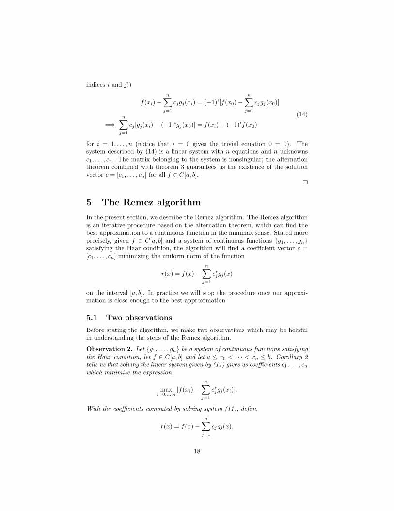
Example 3. Let us find the best linear approximation P (x) = c0 + c1x to thefunction f(x) = ex on [0, 1], i.e. our Haar system is {1, x}. By the alternationtheorem, the error function r = f−P must alternate at least three times. Fromfigure 1 it is clear that the points of alternation are 0, 1 and a point ξ betweenthe two. Furthermore, at the alternation points, the quantity |f(x) − P (x)| isequal to ||r||∞ := ε. We get the following equations:

ε = f(0)− P (0) = 1− c0

−ε = f(ξ)− P (ξ) = eξ − c0 − c1ξ

ε = f(1)− P (1) = e− c0 − c1Moreover, we use the fact that f − P has an extreme value at ξ, that is,

0 = f ′(ξ)− P ′(ξ) = eξ − c1.

Using the first and the fourth equation, we find c0 = 1 − ε and c1 = eξ. Next,we substitute these values for c0 and c1 in the third equation and solve for ξ tofind that ξ = log(e− 1). Lastly we solve the second equation for ε and find that

ε = 2−e+(e−1) log(e−1)2 ≈ 0.106. The best linear approximation to ex on [0, 1] is

P (x) = (e− 1)x+ 1− ε.

16

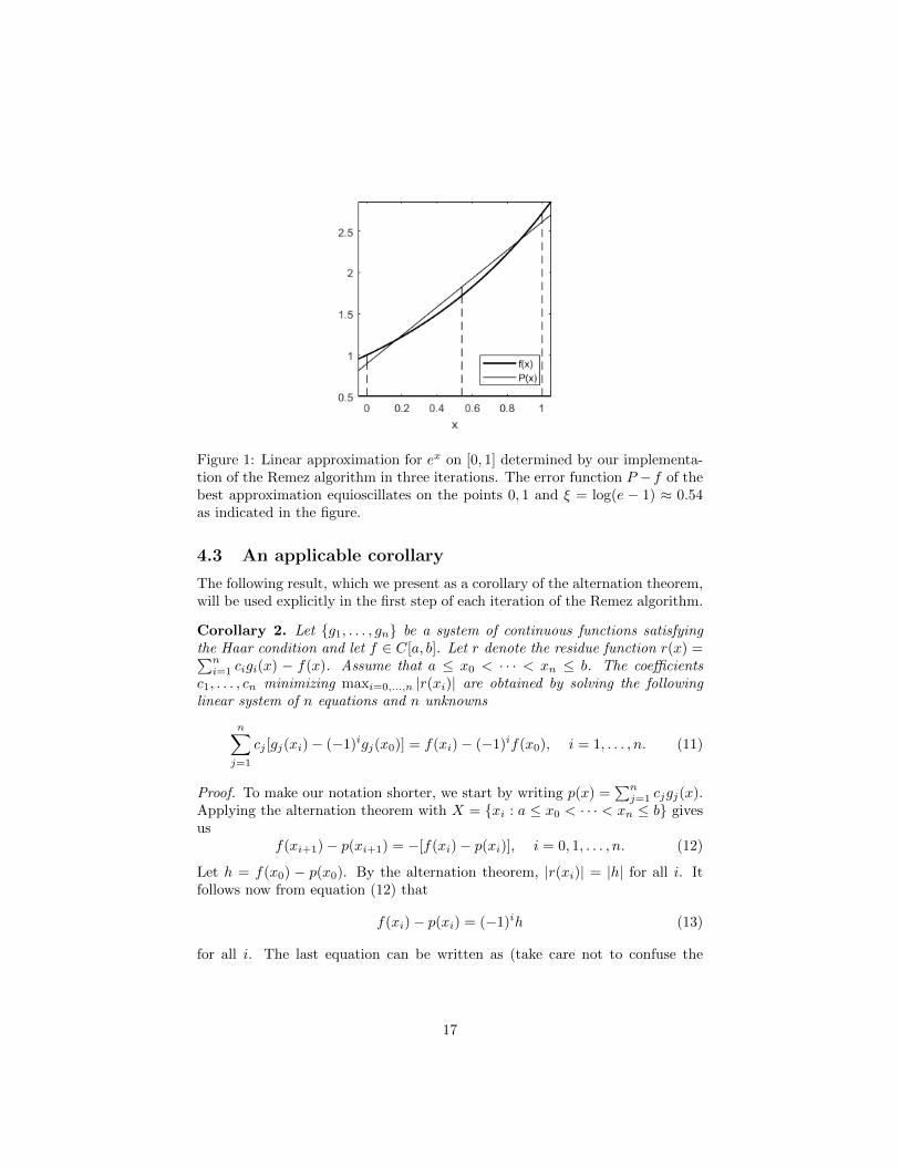
Figure 1: Linear approximation for ex on [0, 1] determined by our implementa-tion of the Remez algorithm in three iterations. The error function P −f of thebest approximation equioscillates on the points 0, 1 and ξ = log(e − 1) ≈ 0.54as indicated in the figure.

4.3 An applicable corollary

The following result, which we present as a corollary of the alternation theorem,will be used explicitly in the first step of each iteration of the Remez algorithm.

Corollary 2. Let {g1, . . . , gn} be a system of continuous functions satisfyingthe Haar condition and let f ∈ C[a, b]. Let r denote the residue function r(x) =∑ni=1 cigi(x) − f(x). Assume that a ≤ x0 < · · · < xn ≤ b. The coefficients

c1, . . . , cn minimizing maxi=0,...,n |r(xi)| are obtained by solving the followinglinear system of n equations and n unknowns

n∑j=1

cj [gj(xi)− (−1)igj(x0)] = f(xi)− (−1)if(x0), i = 1, . . . , n. (11)

Proof. To make our notation shorter, we start by writing p(x) =∑nj=1 cjgj(x).

Applying the alternation theorem with X = {xi : a ≤ x0 < · · · < xn ≤ b} givesus

f(xi+1)− p(xi+1) = −[f(xi)− p(xi)], i = 0, 1, . . . , n. (12)

Let h = f(x0) − p(x0). By the alternation theorem, |r(xi)| = |h| for all i. Itfollows now from equation (12) that

f(xi)− p(xi) = (−1)ih (13)

for all i. The last equation can be written as (take care not to confuse the

17

indices i and j!)

f(xi)−n∑j=1

cjgj(xi) = (−1)i[f(x0)−n∑j=1

cjgj(x0)]

=⇒n∑j=1

cj [gj(xi)− (−1)igj(x0)] = f(xi)− (−1)if(x0)

(14)

for i = 1, . . . , n (notice that i = 0 gives the trivial equation 0 = 0). Thesystem described by (14) is a linear system with n equations and n unknownsc1, . . . , cn. The matrix belonging to the system is nonsingular; the alternationtheorem combined with theorem 3 guarantees us the existence of the solutionvector c = [c1, . . . , cn] for all f ∈ C[a, b].

5 The Remez algorithm

In the present section, we describe the Remez algorithm. The Remez algorithmis an iterative procedure based on the alternation theorem, which can find thebest approximation to a continuous function in the minimax sense. Stated moreprecisely, given f ∈ C[a, b] and a system of continuous functions {g1, . . . , gn}satisfying the Haar condition, the algorithm will find a coefficient vector c =[c1, . . . , cn] minimizing the uniform norm of the function

r(x) = f(x)−n∑j=1

c∗jgj(x)

on the interval [a, b]. In practice we will stop the procedure once our approxi-mation is close enough to the best approximation.

5.1 Two observations

Before stating the algorithm, we make two observations which may be helpfulin understanding the steps of the Remez algorithm.

Observation 2. Let {g1, . . . , gn} be a system of continuous functions satisfyingthe Haar condition, let f ∈ C[a, b] and let a ≤ x0 < · · · < xn ≤ b. Corollary 2tells us that solving the linear system given by (11) gives us coefficients c1, . . . , cnwhich minimize the expression

maxi=0,...,n

|f(xi)−n∑j=1

c∗jgj(xi)|.

With the coefficients computed by solving system (11), define

r(x) = f(x)−n∑j=1

cjgj(x).

18

The alternation theorem tells us that

r(xi) = −r(xi−1) = ±||r||∞, i = 1, . . . , n,

which means that the residue function r has a root in each interval (xi−1, xi).

Observation 3. With the notation from observation 2, let

A = {n∑j=1

c∗jgj(x) : c∗j ∈ R, x ∈ [a, b]}

and let P ∗ be the best approximation to f from the set A. Furthermore, letP (x) =

∑nj=1 cjgj(x) with coefficients as in observation 2. Choose y ∈ [a, b] so

that|r(y)| = max

x∈[a,b]|r(x)| = ||r||∞.

In [1, p. 86] it is found that

||f − P ||∞ ≤ ||f − P ∗||∞ + δ,

whereδ = |r(y)| − |r(x0)|.

Recall that |r(x0)| = · · · = |r(xn)| by the alternation theorem. In the algorithmwhich we will state below, we will stop iterating once δ is small enough, be-cause this tells us that the computed approximation is close enough to the bestapproximation from A.

5.2 Statement of the Remez algorithm

Input: A function f ∈ C[a, b], functions g1, . . . , gn ∈ C[a, b] so that the system{g1, . . . , gn} satisfying the Haar condition, the interval [a, b], an initial reference{x0, . . . , xn}, where a ≤ x0 < · · · < xn ≤ b and a constant δ > 0 for the stoppingcriterion. We describe the steps of a generic iteration k.

Step 1: If k = 1, the reference {x0, . . . , xn} comes from the input, otherwiseit is defined in the previous iteration. Solve linear system (11) to computecoefficients c1, . . . , cn minimizing the expression

maxi=0,...,n

|f(xi)−n∑j=1

c∗jgj(xi)|.

Define r(x) = f(x)−∑nj=1 cjgj(x) with the coefficients c1, . . . , cn just computed.

Note: The function P (x) =∑nj=1 cjgj(x) is the approximation for f obtained

in the present iteration, iteration k. The upcoming steps only influence theapproximation computed in the next iteration, iteration k + 1.

19

Stopping criterion: Find y ∈ [a, b] so that

|r(y)| = maxx∈[a,b]

|r(x)|.

Stop iterating if|r(y)| − |r(x0)| < δ.

Otherwise continue in step 2.

Step 2: Define z0 = a, zn+1 = b and find a root zi in (xi−1, xi) for alli = 1, . . . , n. The existence of these roots was mentioned in observation 2.

Step 3: Let σi = sgn r(xi). For all i = 0, . . . , n, find yi ∈ [zi, zi+1] whereσir(y) is a maximum with the property that σir(yi) ≥ σir(xi). Replace thereference {x0, . . . , xn} by {y0, . . . , yn}.

Step 4: In the stopping criterion we computed y ∈ [a, b] so that

|r(y)| = maxx∈[a,b]

|r(x)|.

If|r(y)| = max

i=0,...,n|r(yi)|,

go to step 1 of iteration k + 1 with the reference defined in step 3. If

|r(y)| > maxi=0,...,n

|r(yi)|,

include the point y in the set {y0, . . . , yn} and put it in the right position sothat the elements are still in ascending order. Lastly, remove one of the yi insuch a way that r(x) still alternates in sign on the resulting set. A descriptionof how to accomplish this is given in appendix B. The resulting set is the newreference. Start in step 1 of iteration k + 1 with this new reference.

5.3 A visualization of the reference adjustment

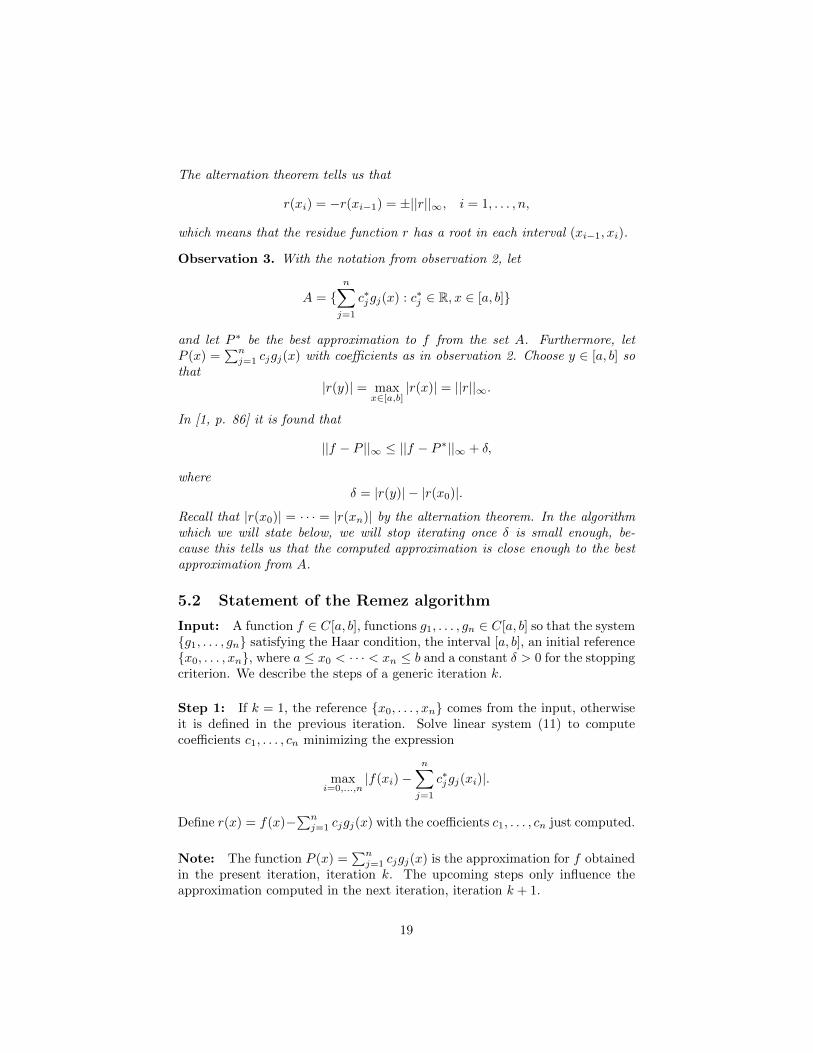
In figure 2 it can be seen how the reference is adjusted in an iteration of theRemez algorithm. The figure shows the residue function in the first iterationfor determining a second degree polynomial approximation for the function

f(x) = e−x sin(3πx) cos(3πx)| sin(2πx)|

on the interval [0, 1]. Notice that for a second degree polynomial approximation,our Haar system is {1, x, x2}, that is, we have 3 basis elements. Thereforeour initial reference must consist of 4 points. As initial reference we chose 4equispaced nodes in [0.2, 0.8]. This choice for f and for the initial reference is aresult of trial and error; the goal was to obtain plots in which it is visable howthe reference is adjusted in each step of an iteration.

20

Figure 2: Residue function and reference points in steps 2, 3, 4 of the first it-eration of the Remez algorithm for determining a second degree polynomialapproximation to the function f(x) = e−x sin(3πx) cos(3πx)| sin(2πx)|. In eachstep the locations of the reference points and the numbers z0, . . . , z5 are indi-cated by stars and dots, respectively. In step 2, equioscillations on the initialreference are visible. In step 3, the reference points are re-located to the positionof local maxima in accordance with the description of the algorithm. In the laststep, the location of the global maximum of |r| is included into the reference andone point is removed in the way described in step 4 of the statement of the al-gorithm. The residue function still alternates in sign on the resulting reference.The figure was created using our implementation of the Remez algorithm.

21

6 Testing our implementation of the Remez al-gorithm

In this section, we discuss several results obtained by using our Matlab imple-mentation of the Remez algorithm. We discuss situations in which the imple-mentation works well and discuss in what cases it may not give satisfactoryresults. We start by discussing some of the choices we made when making ourimplementation.

6.1 Comments about the implementation

Considerations

• Instead of letting the algorithm stop when δ = ||r||∞ − |r(x0)| is smallenough, we will let it stop when |δ| is small enough. Theoretically, δ ≥ 0,but because in the algorithm ||r||∞ becomes close to |r(x0)|, situationsmay occur where δ becomes less than 0 due to computational errors.

• We use Matlab’s built-in function fminbnd to locate local maxima of theresidue function. For example, a maximum of a function f can be foundon an interval by minimizing −f . In the third step of the algorithm itis necessary to find yi ∈ [zi, zi+1] where σir(y) is a maximum with theproperty that σir(yi) ≥ σir(xi). If fminbnd does not locate a maximumwith this property, but e.g. a lower local maximum, we start a brute-forcesearch for a maximum satsifying σir(yi) ≥ σir(xi). If no such maximumcan be found, it must be that σir(xi) is close to the absolute maximumon [zi, zi+1] and we choose yi = xi.

• We have chosen z0 = a and zn+1 = b. These points are not generallyzeroes of the residue function and in the search for a maximum in theintervals [z0, z1] and [zn, zn+1] we also evaluate the points z0 and zn+1,respectively.

• The global maximum of the residue function is located by a brute-forcesearch. We evaluate the residue function in 10000 equispaced steps be-tween [0, 1] and find the maximum of these evaluations. The brute-forcesearch should find the x−coordinate xmax of the maximum with an errorof at most 10−4.

Accuracy of the brute-force search We can use the mean value theorem(MVT) [13, p. 138] to say something about the accuracy of the value for ||r||∞found by use of our brute-force method, where r is again a residue function.Suppose that x1 is the x−coordinate of the maximum found by the brute-force search and x2 is the x−coordinate of the exact location of the maximum.Recall that the residue function r is continuous. Under the condition that

22

r is differentiable on (x1, x2), application the MVT and using the fact that|x1 − x2| ≤ 10−4 tells us that there exists a point c ∈ (x1, x2) such that

|r(x2)− r(x1)| = |r′(c)| · |x2 − x1|≤ |r′(c)| · 10−4.

(15)

If then, for example |r′(x)| ≤ 1 for x in a neighbourhood of 10−4 around thelocation of the true maximum, we can conclude that the approximated valuefor ||r||∞ differs at most by a value of 10−4 from the true value.

Assuming that r is differentiable, it can be noticed that in a small neighbour-hood around the location of the maximum of |r|, |r′| would only attain a valueas large as 1 in rather extreme cases, e.g. when the plot of the residue functionshows a sharp peak. High values for |r′| at the endpoints of the interval of ap-proximation should not cause problems because the brute-force search methodevaluates r at these endpoints. Inspection of the plot of the residue function canindicate if it is reasonable to trust the value found for ||r||∞. Unless indicatedotherwise, we will, for the remainder of this section, accept the values found for||r||∞ by the brute-force method without further comments.

6.2 Examples

Comparison with two analytically determined results We compare twolinear approximations determined by our implementation with two analyticallydetermined best linear approximations, see table 1. Here, n is the number ofiterations used, P ∗r is the approximation determined by the Remez algorithmand P ∗a is the analytically determined best approximation.

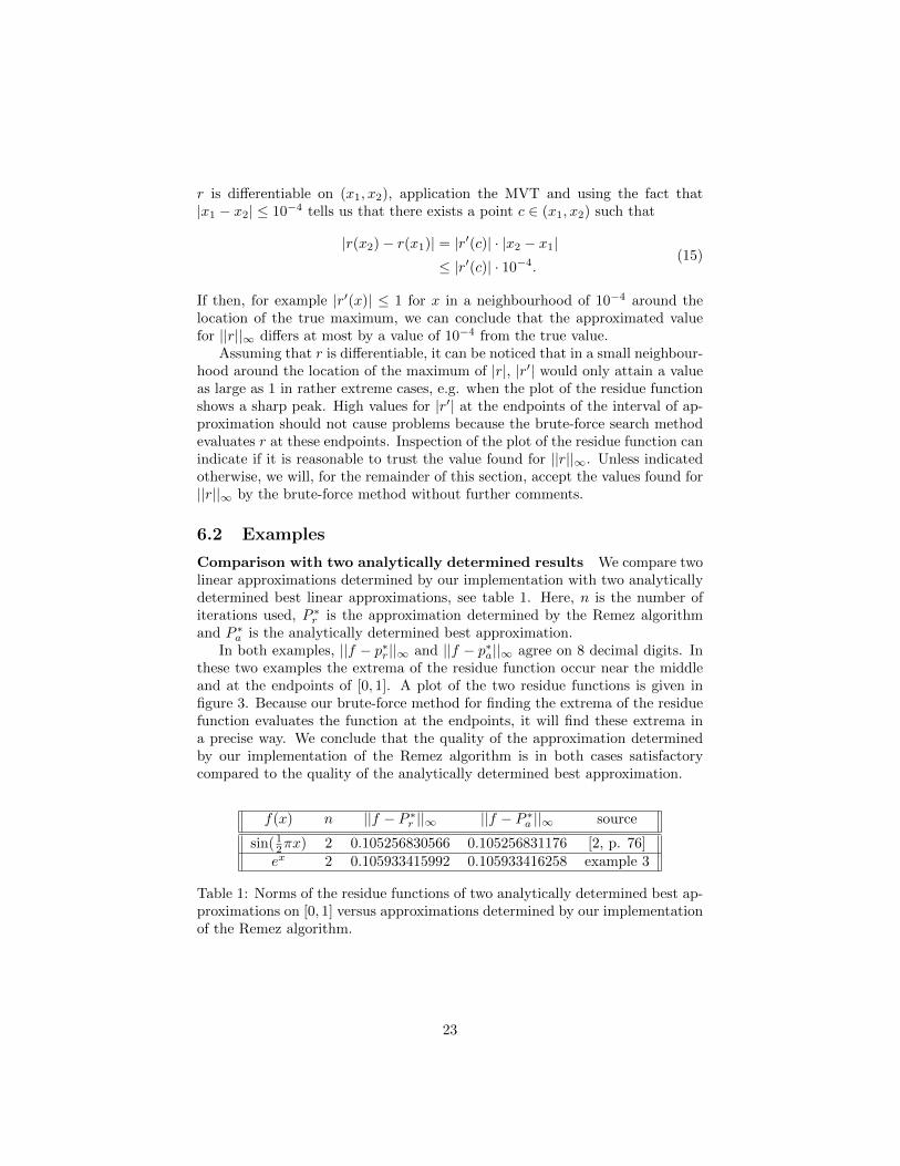
In both examples, ||f − p∗r ||∞ and ||f − p∗a||∞ agree on 8 decimal digits. Inthese two examples the extrema of the residue function occur near the middleand at the endpoints of [0, 1]. A plot of the two residue functions is given infigure 3. Because our brute-force method for finding the extrema of the residuefunction evaluates the function at the endpoints, it will find these extrema ina precise way. We conclude that the quality of the approximation determinedby our implementation of the Remez algorithm is in both cases satisfactorycompared to the quality of the analytically determined best approximation.

f(x) n ||f − P ∗r ||∞ ||f − P ∗a ||∞ source

sin( 12πx) 2 0.105256830566 0.105256831176 [2, p. 76]ex 2 0.105933415992 0.105933416258 example 3

Table 1: Norms of the residue functions of two analytically determined best ap-proximations on [0, 1] versus approximations determined by our implementationof the Remez algorithm.

23

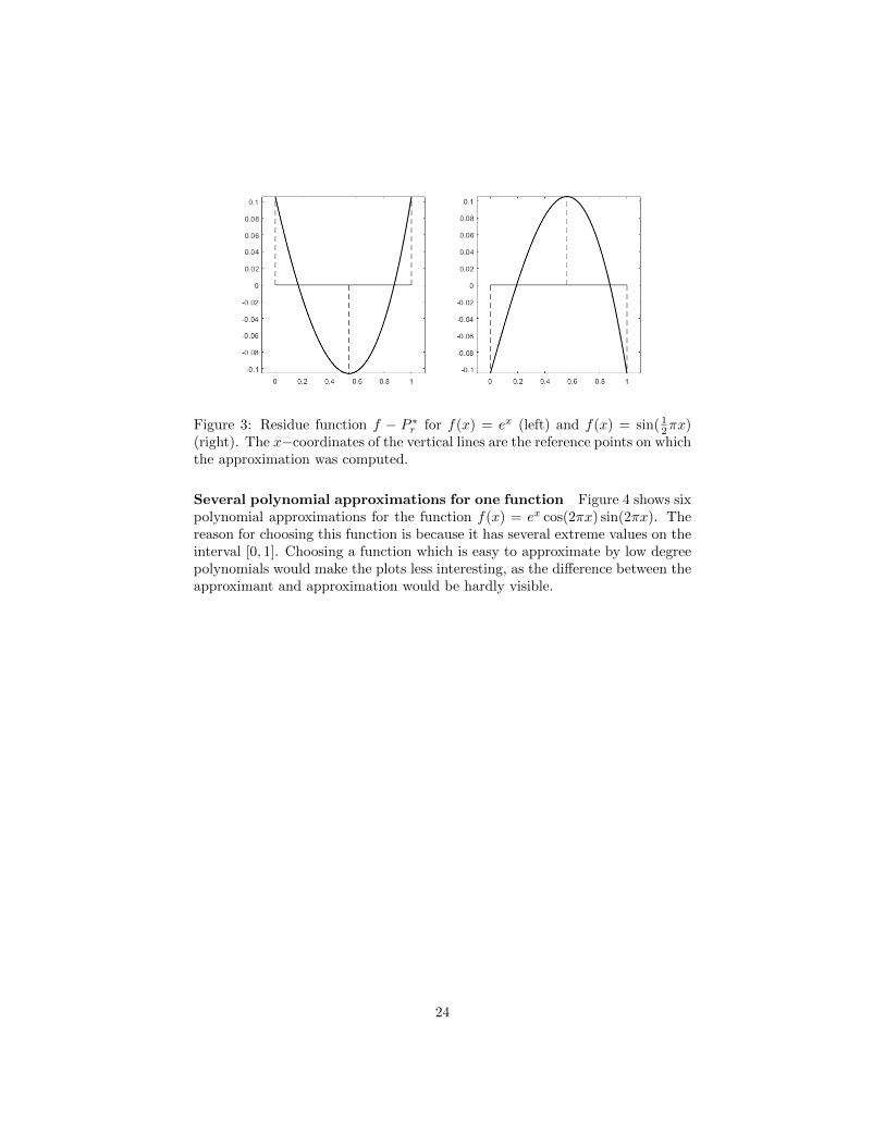
Figure 3: Residue function f − P ∗r for f(x) = ex (left) and f(x) = sin( 12πx)

(right). The x−coordinates of the vertical lines are the reference points on whichthe approximation was computed.

Several polynomial approximations for one function Figure 4 shows sixpolynomial approximations for the function f(x) = ex cos(2πx) sin(2πx). Thereason for choosing this function is because it has several extreme values on theinterval [0, 1]. Choosing a function which is easy to approximate by low degreepolynomials would make the plots less interesting, as the difference between theapproximant and approximation would be hardly visible.

24

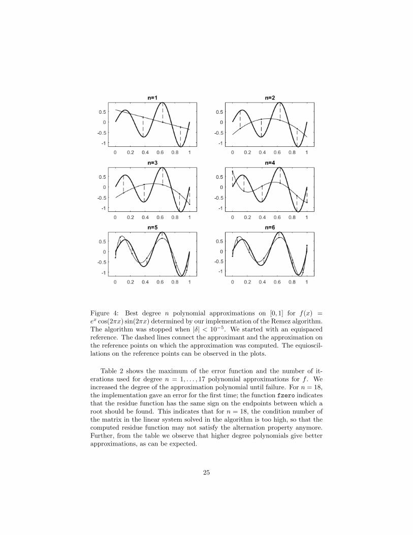
Figure 4: Best degree n polynomial approximations on [0, 1] for f(x) =ex cos(2πx) sin(2πx) determined by our implementation of the Remez algorithm.The algorithm was stopped when |δ| < 10−5. We started with an equispacedreference. The dashed lines connect the approximant and the approximation onthe reference points on which the approximation was computed. The equioscil-lations on the reference points can be observed in the plots.

Table 2 shows the maximum of the error function and the number of it-erations used for degree n = 1, . . . , 17 polynomial approximations for f . Weincreased the degree of the approximation polynomial until failure. For n = 18,the implementation gave an error for the first time; the function fzero indicatesthat the residue function has the same sign on the endpoints between which aroot should be found. This indicates that for n = 18, the condition number ofthe matrix in the linear system solved in the algorithm is too high, so that thecomputed residue function may not satisfy the alternation property anymore.Further, from the table we observe that higher degree polynomials give betterapproximations, as can be expected.

25

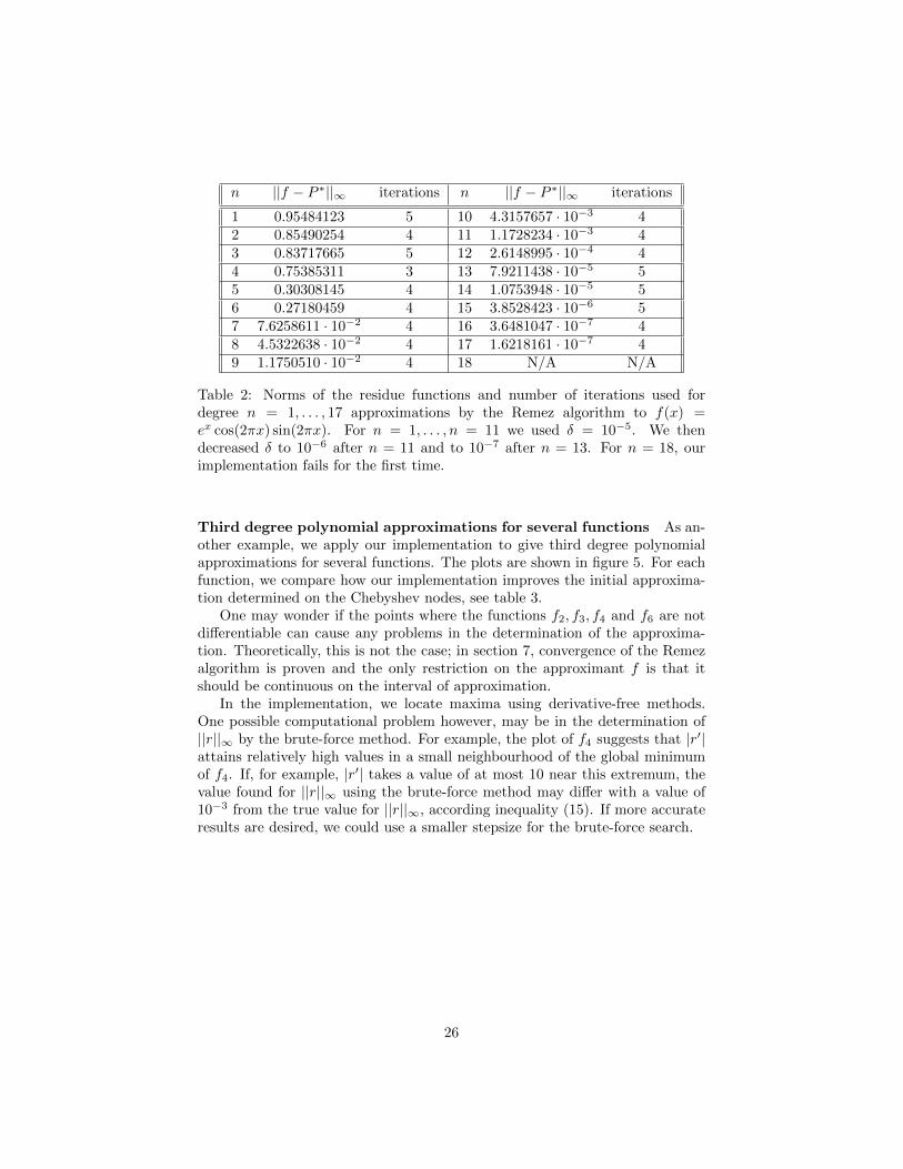
n ||f − P ∗||∞ iterations n ||f − P ∗||∞ iterations

1 0.95484123 5 10 4.3157657 · 10−3 42 0.85490254 4 11 1.1728234 · 10−3 43 0.83717665 5 12 2.6148995 · 10−4 44 0.75385311 3 13 7.9211438 · 10−5 55 0.30308145 4 14 1.0753948 · 10−5 56 0.27180459 4 15 3.8528423 · 10−6 57 7.6258611 · 10−2 4 16 3.6481047 · 10−7 48 4.5322638 · 10−2 4 17 1.6218161 · 10−7 49 1.1750510 · 10−2 4 18 N/A N/A

Table 2: Norms of the residue functions and number of iterations used fordegree n = 1, . . . , 17 approximations by the Remez algorithm to f(x) =ex cos(2πx) sin(2πx). For n = 1, . . . , n = 11 we used δ = 10−5. We thendecreased δ to 10−6 after n = 11 and to 10−7 after n = 13. For n = 18, ourimplementation fails for the first time.

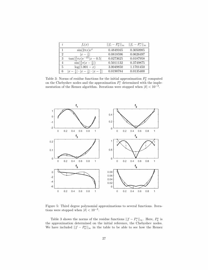
Third degree polynomial approximations for several functions As an-other example, we apply our implementation to give third degree polynomialapproximations for several functions. The plots are shown in figure 5. For eachfunction, we compare how our implementation improves the initial approxima-tion determined on the Chebyshev nodes, see table 3.

One may wonder if the points where the functions f2, f3, f4 and f6 are notdifferentiable can cause any problems in the determination of the approxima-tion. Theoretically, this is not the case; in section 7, convergence of the Remezalgorithm is proven and the only restriction on the approximant f is that itshould be continuous on the interval of approximation.

In the implementation, we locate maxima using derivative-free methods.One possible computational problem however, may be in the determination of||r||∞ by the brute-force method. For example, the plot of f4 suggests that |r′|attains relatively high values in a small neighbourhood of the global minimumof f4. If, for example, |r′| takes a value of at most 10 near this extremum, thevalue found for ||r||∞ using the brute-force method may differ with a value of10−3 from the true value for ||r||∞, according inequality (15). If more accurateresults are desired, we could use a smaller stepsize for the brute-force search.

26

i fi(x) ||fi − P ∗0 ||∞ ||fi − P ∗r ||∞1 sin(2πx)ex 0.4849165 0.30509852 |x− 1

2 | 0.0818596 0.06264973 tan( 2

5πx)e−2x|x− 0.5| 0.0273625 0.01879584 sin( 3

2π|x−12 |) 0.5011132 0.3749875

5 log(1.001− x) 3.0049850 1.17014506 |x− 1

4 | · |x−12 | · |x−

34 | 0.0190784 0.0135400

Table 3: Norms of residue functions for the initial approximation P ∗0 computedon the Chebyshev nodes and the approximation P ∗r determined with the imple-mentation of the Remez algorithm. Iterations were stopped when |δ| < 10−3.

Figure 5: Third degree polynomial approximations to several functions. Itera-tions were stopped when |δ| < 10−3.

Table 3 shows the norms of the residue functions ||f − P ∗r ||∞. Here, P ∗0 isthe approximation determined on the initial reference, the Chebyshev nodes.We have included ||f − P ∗0 ||∞ in the table to be able to see how the Remez

27

algorithm improves the first approximation on the Chebyshev nodes. In theseexamples, it can be seen that the Remez algorithm improves the approximationon the Chebyshev nodes by a factor between 1.3 and 2.6. Excluding f5, theapproximation is improved by a factor between 1.3 and 1.6 for each example.

In each of the examples, the approximation on the reference determined bythe Remez algorithm is an improvement compared to the initial approximationon the Chebyshev nodes, as can be seen in table 3.

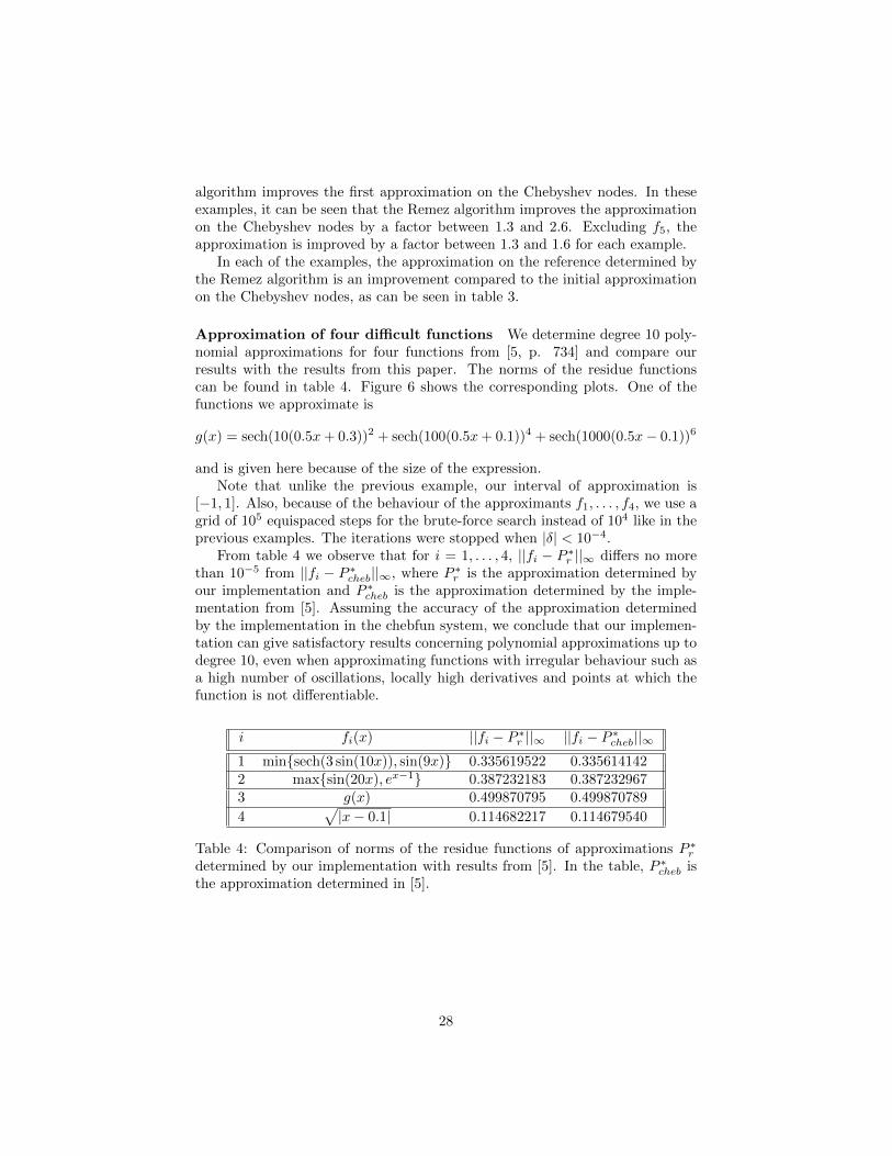
Approximation of four difficult functions We determine degree 10 poly-nomial approximations for four functions from [5, p. 734] and compare ourresults with the results from this paper. The norms of the residue functionscan be found in table 4. Figure 6 shows the corresponding plots. One of thefunctions we approximate is

g(x) = sech(10(0.5x+ 0.3))2 + sech(100(0.5x+ 0.1))4 + sech(1000(0.5x− 0.1))6

and is given here because of the size of the expression.Note that unlike the previous example, our interval of approximation is

[−1, 1]. Also, because of the behaviour of the approximants f1, . . . , f4, we use agrid of 105 equispaced steps for the brute-force search instead of 104 like in theprevious examples. The iterations were stopped when |δ| < 10−4.

From table 4 we observe that for i = 1, . . . , 4, ||fi − P ∗r ||∞ differs no morethan 10−5 from ||fi − P ∗cheb||∞, where P ∗r is the approximation determined byour implementation and P ∗cheb is the approximation determined by the imple-mentation from [5]. Assuming the accuracy of the approximation determinedby the implementation in the chebfun system, we conclude that our implemen-tation can give satisfactory results concerning polynomial approximations up todegree 10, even when approximating functions with irregular behaviour such asa high number of oscillations, locally high derivatives and points at which thefunction is not differentiable.

i fi(x) ||fi − P ∗r ||∞ ||fi − P ∗cheb||∞1 min{sech(3 sin(10x)), sin(9x)} 0.335619522 0.3356141422 max{sin(20x), ex−1} 0.387232183 0.3872329673 g(x) 0.499870795 0.499870789

4√|x− 0.1| 0.114682217 0.114679540

Table 4: Comparison of norms of the residue functions of approximations P ∗rdetermined by our implementation with results from [5]. In the table, P ∗cheb isthe approximation determined in [5].

28

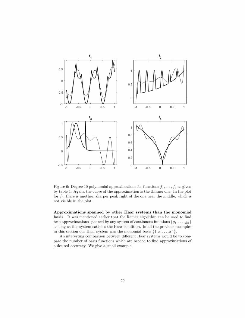
Figure 6: Degree 10 polynomial approximations for functions f1, . . . , f4 as givenby table 4. Again, the curve of the approximation is the thinner one. In the plotfor f3, there is another, sharper peak right of the one near the middle, which isnot visible in the plot.

Approximations spanned by other Haar systems than the monomialbasis It was mentioned earlier that the Remez algorithm can be used to findbest approximations spanned by any system of continuous functions {g1, . . . , gn}as long as this system satisfies the Haar condition. In all the previous examplesin this section our Haar system was the monomial basis {1, x, . . . , xn}.

An interesting comparison between different Haar systems would be to com-pare the number of basis functions which are needed to find approximations ofa desired accuracy. We give a small example.

29

For the Haar systems

H1 = {1, x, x2, . . . , xn}H2 = {1, e0.5x, ex, . . . , e0.5nx}H3 = {1, ex, e2x, . . . , enx},

(16)

table 5 shows how many basis elements are needed from the bases H1, H2, H3

in order to approximate the given functions fi, i = 1, . . . , 6 in such a way that||ri||∞ < 0.05, where ri is the residue function corresponding to the approxima-tion for fi. The fact that H2 and H3 satisfy the Haar condition is mentionedin [7, p. 297].

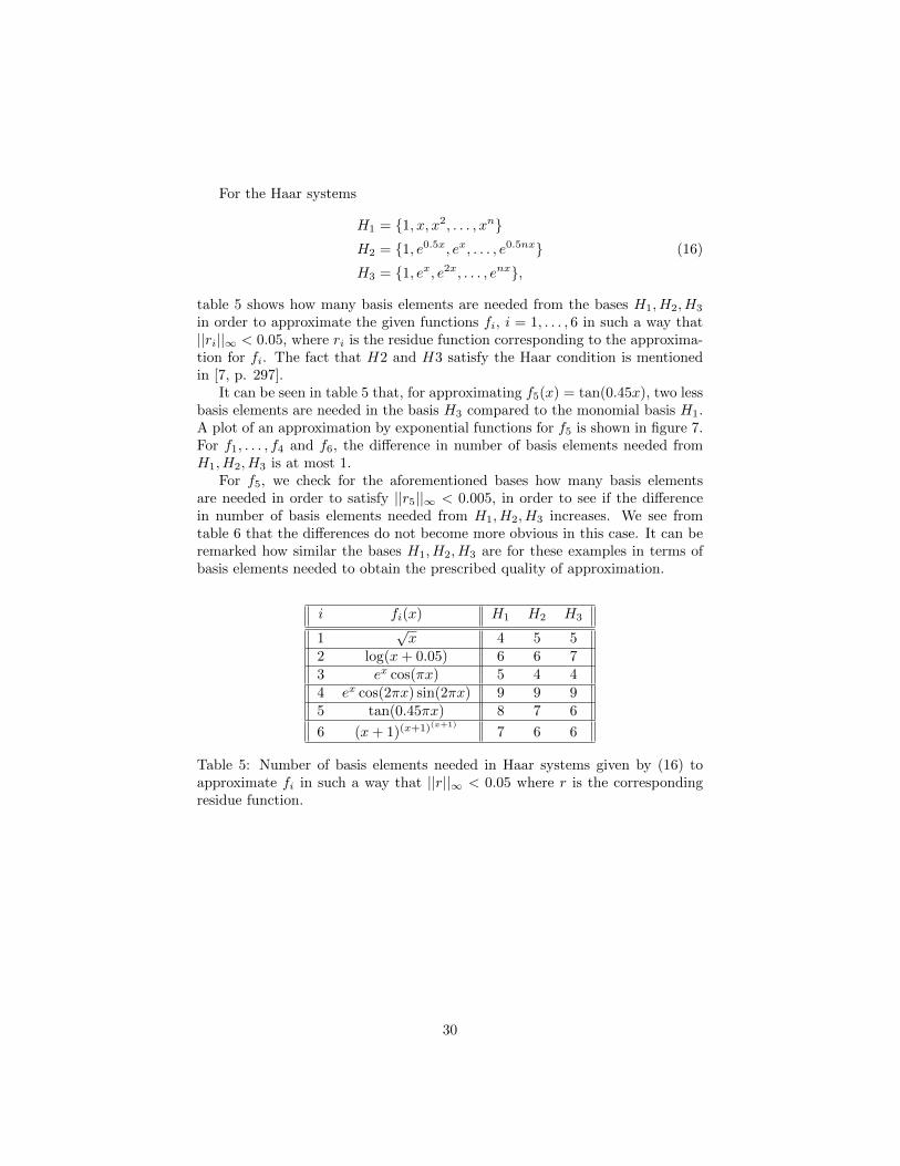
It can be seen in table 5 that, for approximating f5(x) = tan(0.45x), two lessbasis elements are needed in the basis H3 compared to the monomial basis H1.A plot of an approximation by exponential functions for f5 is shown in figure 7.For f1, . . . , f4 and f6, the difference in number of basis elements needed fromH1, H2, H3 is at most 1.

For f5, we check for the aforementioned bases how many basis elementsare needed in order to satisfy ||r5||∞ < 0.005, in order to see if the differencein number of basis elements needed from H1, H2, H3 increases. We see fromtable 6 that the differences do not become more obvious in this case. It can beremarked how similar the bases H1, H2, H3 are for these examples in terms ofbasis elements needed to obtain the prescribed quality of approximation.

i fi(x) H1 H2 H3

1√x 4 5 5

2 log(x+ 0.05) 6 6 73 ex cos(πx) 5 4 44 ex cos(2πx) sin(2πx) 9 9 95 tan(0.45πx) 8 7 6

6 (x+ 1)(x+1)(x+1)

7 6 6

Table 5: Number of basis elements needed in Haar systems given by (16) toapproximate fi in such a way that ||r||∞ < 0.05 where r is the correspondingresidue function.

30

i fi(x) H1 H2 H3

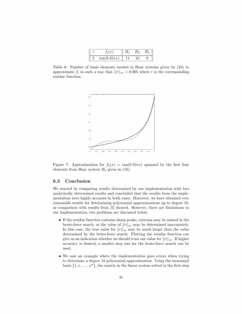
5 tan(0.45πx) 11 10 9

Table 6: Number of basis elements needed in Haar systems given by (16) toapproximate fi in such a way that ||r||∞ < 0.005 where r is the correspondingresidue function.

Figure 7: Approximation for f5(x) = tan(0.45πx) spanned by the first fourelements from Haar system H2 given in (16).

6.3 Conclusion

We started by comparing results determined by our implementation with twoanalytically determined results and concluded that the results from the imple-mentation were highly accurate in both cases. Moreover, we have obtained veryreasonable results for determining polynomial approximations up to degree 10,as comparison with results from [5] showed. However, there are limitations toour implementation; two problems are discussed below.

• If the residue function contains sharp peaks, extrema may be missed in thebrute-force search, or the value of ||r||∞ may be determined inaccurately.In this case, the true value for ||r||∞ may be much larger than the valuedetermined by the brute-force search. Plotting the residue function cangive us an indication whether we should trust our value for ||r||∞. If higheraccuracy is desired, a smaller step size for the brute-force search can beused.

• We saw an example where the implementation gave errors when tryingto determine a degree 18 polynomial approximation. Using the monomialbasis {1, x, . . . , xn}, the matrix in the linear system solved in the first step

31

of the algorithm, is the Vandermonde matrix. It is known that generallythe condition number of this matrix increases exponentially as n increases[5, p. 728]. If the condition number is too high, the numerical solution ofthe linear system will be inaccurate. In the implementation described in[5], the problem of an increasing condition number is avoided by a suitableadjustment of the basis in each iteration. For details, see [5, p. 728].

7 Proof of convergence of the Remez algorithm

Our final goal is to give a proof of convergence of the Remez algorithm. Itis known for many approximants the convergence of the Remez algorithm isquadratic [2, p. 98]. We will not prove this fact here, but instead conclude bypresenting a proof of the linear convergence, which is valid for any continuousapproximant. Before doing so, we will need to extend the theory presented inthe first sections slightly more by proving the theorem of de La Vallee-Poussinand the strong unicity theorem. First we prove a short lemma about the Haarcondition.

Lemma 3. The system of continuous functions {g1, . . . , gn} satisfies the Haarcondition if and only if no nontrivial generalized polynomial

∑ni=1 cigi has more

than n− 1 distinct roots.

Proof. ( =⇒ ) Assume the Haar condition is satisfied. Then the matrix in theequation g1(x1) . . . gn(x1)

.... . .

...g1(xn) . . . gn(xn)

c1...cn

=

0...0

(17)

is nonsingular whenever x1, . . . , xn are all distinct. In this case, the only solutionis the trivial solution c1 = · · · = cn = 0, that is, no nontrivial generalizedpolynomial can have n or more roots.( ⇐= ) By contraposition. Assume the Haar condition is not satisfied. Thenthere exist x1, . . . , xn, all dinstinct, so that the matrix in equation (17) hasrank < n. In this case, a nontrivial solution vector [c1, . . . , cn]ᵀ exists, hencethe nontrivial generalized polynomial

∑ni=1 cigi has the roots x1, . . . , xn.

7.1 Theorem of de La Vallee Poussin and the strong unic-ity theorem

The following theorem gives a lower bound for the largest deviation betweenthe approximant and the best minimax approximation.

Theorem 12. (de La Vallee Poussin) Assume the system of continuous func-tions {g1, . . . , gn} satisfies the Haar condition. Define

E(f) = inf ||P − f ||∞,

32

where P ranges over all generalized polynomials∑ni=1 cigi. Let P be a gener-

alized polynomial such that f − P is alternately positive and negative at n + 1consecutive points xi ∈ [a, b]. Then

E(f) ≥ mini|f(xi)− P (xi)|.

Proof. Assume for contradiction that

E(f) < mini|f(xi)− P (xi)|.

Then there exists a generalized polynomial P0 so that

maxx∈[a,b]

|f(x)− P0(x)| < mini|f(xi)− P (xi)|.

Now we write P0 − P = (f − P ) − (f − P0). From the inequality above itfollows that the generalized polynomial P0 − P alternates in sign at the n + 1consecutive points xi. But then P0 − P has n roots, contradicting the lemmawe just proved.

Theorem 13. (Strong unicity) Assume the system of continuous functions{g1, . . . , gn} satisfies the Haar condition and let P ∗ be the best generalized poly-nomial approximation (spanned by g1, . . . , gn) to f ∈ C[a, b]. Then there exists aconstant γ(f) > 0 such that for all other generalized polynomials P =

∑ni=1 cigi,

we have||f − P ||∞ ≥ ||f − P ∗||∞ + γ||P ∗ − P ||∞.

Proof. First, let us consider the case where ||f −P ∗||∞ = 0. Then we apply thetriangle inequality to see

||P − P ∗||∞ = ||(f − P )− (f − P ∗)||∞≤ ||f − P ||∞ + ||f − P ∗||∞= ||f − P ||∞.

In this case we choose γ = 1.Assume now that ||f − P ∗|| > 0. Let r(x) = f(x) − P ∗(x). Since P ∗

is assumed to be the best minimax approximation to f , the characterizationtheorem tells us that 0 is contained in the convex hull of the set

U = {r(x)[g1(x), . . . , gn(x)]ᵀ : |r(x)| = ||r||∞}.

Hence, we may write

0 =

n∑i=0

θir(xi)[g1(xi), . . . , gn(xi)]ᵀ,

with θi ≥ 0 and∑θi = 1. Now let σi = sgn(r(xi)) for i = 0, . . . , n. After

rescaling and possibly re-labeling, we may write

0 =

k∑i=0

θiσi[g1(xi), . . . , gn(xi)]ᵀ

33

with θi > 0. That is, an equation

0 =

k∑i=0

θiσigj(xi)

holds for j = 1, . . . , n. By the Haar condition, k ≥ n. Caratheodory’s theoremtells us that k ≤ n and we conclude k = n.

Let Q(x) =∑nj=1 cjgj(x) be a generalized polynomial with norm 1. Then

n∑i=0

θiσiQ(xi) =

n∑i=0

θiσi

n∑j=1

cjgj(xi)

=

n∑j=1

cj

n∑i=0

θiσigj(xi)

= 0.

By the Haar condition, lemma 3 tells us that the σiQ(xi) cannot all be zero.Hence, at least one of the σiQ(xi) must be strictly positive. This implies thatmaxi σiQ(xi) is a strictly positive function of Q. The set

{Q(x) =

n∑j=1

cjgj(x) : ||Q||∞ = 1}

is compact as it is a closed and bounded subset of the finite dimensional linearspace spanned by {g1, . . . , gn}. Thus the number

γ = min||Q||∞=1

maxiσiQ(xi) (18)

is strictly positive as it is the minimum of a strictly positive continuous functionon a compact set. Now, let P be any generalized polynomial. There are twocases. If P = P ∗, the inequality we want to prove follows trivially since in thiscase we may choose γ arbitrarily. Otherwise, the generalized polynomial

Q =P ∗ − P||P ∗ − P ||∞

has norm 1. By the definition of γ in (18), we have σiQ(xi) ≥ γ for some indexi. Consequently, for this index, σi(P

∗ − P )(xi) ≥ γ||P ∗ − P ||∞ and hence,

||f − P ||∞ ≥ σi(f − P )(xi)

= σi(f − P ∗)(xi) + σi(P∗ − P )(xi)

≥ ||f − P ∗||∞ + γ||P ∗ − P ||∞.

In the last step we used the fact that xi is an element satisfying f(xi)−P ∗(xi) =r(xi) = ±||r||∞ and hence σir(xi) = ||r||∞.

34

7.2 Proof of convergence

Theorem 14. (Convergence of the Remez algorithm) Let P k denote the gen-eralized polynomial obtained in iteration k in the Remez algorithm and let P ∗

be the best minimax approximation spanned by the corresponding Haar system.Then an inequality of the form

||P k − P ∗||∞ ≤ Aθk

with 0 < θ < 1 holds, which means that P k → P ∗ uniformly.

Proof. We use the notation from the description of the Remez algorithm insection 5. At the end of iteration k, define

α = mini|r(xi)| = max

i|r(xi)|,

β = maxi|r(yi)| = ||r||∞,

γ = mini|r(yi)|.

Notice here that the definition of α is justified because in the first step of theiteration, the best approximation on the reference {x0, . . . , xn} is computed. Bythe alternation theorem, the absolute values of the r(xi)’s are all equal. Noticefurthermore that in the last step of the iteration, an element y ∈ [a, b] satisfyingr(y) = ||r||∞ was included in the new reference {y0, . . . , yn}, justifying thedefinition of β. The corresponding quantities obtained in the next iteration aredenoted by α′, β′ and γ′.

Define β∗ = ||f −P ∗||∞, where P ∗ is the best minimax approximation as inthe statement of the theorem. By the theorem of de La Vallee Poussin, β∗ ≥ γ.It is clear that β ≥ β∗. From the definition of the new reference {y0, . . . , yn} itis furthermore clear that γ ≥ α. This gives us the following:

α ≤ γ ≤ β∗ ≤ β. (19)

In the beginning of the next iteration, the vector c′ = [c′1, . . . , c′n]ᵀ minimizing

maxi|f(yi)−

n∑j=1

c′jgj(yi)|

is computed. By (13) in the proof of corollary 2, the coefficient vector c′ isobtained by solving the linear system

(−1)ih+

n∑j=1

c′jgj(yi) = f(yi), i = 0, . . . , n

for the unknowns h and c′1, . . . , c′n, where h = r(y0). The matrix of this system

is nonsingular; in the proof of corollary 2 we observed that the solution vector

35

c′ exists and is unique. The constant h is then determined uniquely by c′. Wewrite this system as matrix-vector equation:

1 g1(y0) . . . gn(y0)−1 g1(y1) . . . gn(y1)...

.... . .

...(−1)n g1(yn) . . . gn(yn)

hc′1...c′n

=

f(y0)f(y1)

...f(yn)

.Next, we use Cramer’s rule to solve for h and obtain

h =

∣∣∣∣∣∣∣∣∣f(y0) g1(y0) . . . gn(y0)f(y1) g1(y1) . . . gn(y1)

......

. . ....

f(yn) g1(yn) . . . gn(yn)

∣∣∣∣∣∣∣∣∣÷∣∣∣∣∣∣∣∣∣

1 g1(y0) . . . gn(y0)−1 g1(y1) . . . gn(y1)...

.... . .

...(−1)n g1(yn) . . . gn(yn)

∣∣∣∣∣∣∣∣∣ .Denote the minors corresponding to the column with ±1 in the determinant

in the denominator by Mi. The solution for h can then be written as

h =

∑ni=0 f(yi)Mi(−1)i∑n

j=0Mj. (20)

If f itself in (20) is replaced by a generalized polynomial P =∑nj=1 ajgj , then

the approximation on the reference {y0, . . . , yn} is exact and hence h = 0, whichmeans that

n∑i=0

P (yi)Mi(−1)i = 0.

This shows that in (20), the approximant f(x) may be replaced by

r(x) = f(x)−n∑j=1

c′jgj(x),

leaving h unchanged. We use the fact that the r(yi)’s alternate in sign to seethat

n∑i=0

r(yi)(−1)iMi = ±n∑i=0

|r(yi)|Mi. (21)

Furthermore, because y0 < · · · < yn and because the Haar condition is satisfiedby {g1, . . . , gn}, lemma 1 tells us that all the minors Mi have the same sign.Hence, combining (21) with the expression for h in (20), we find that

α′ = |h| =∑ni=0 |Mi||r(yi)|∑n

j=0 |Mj |. (22)

Now let

θi =|Mi|∑nj=0 |Mj |

. (23)

36

Notice here that θi ∈ (0, 1) because there are at least two minors. Combine (22)and (23) to obtain

α′ =

n∑i=0

θi|r(yi)|

≥n∑i=0

θi minj|r(yj)|

=

n∑i=0

θiγ

= γ

(24)

where we used in the last step the fact that∑ni=0 θi = 1.

Assume for now that throughout the iterations of the algorithm, the numbersθi remain larger than a fixed constant 1−θ > 0. This assumption will be justifiedin a lemma after this proof. We establish the following inequalities.

γ′ − γ ≥ α′ − γ using γ′ ≥ α′ from (24)

=

n∑i=0

θi(|r(yi)| − γ) using∑

θi = 1

≥ miniθi(β − γ) where β = max

i|r(yi)|

≥ (1− θ)(β − γ) because θi ≥ 1− θ for all i (25)

≥ (1− θ)(β∗ − γ) since β ≥ β∗ by (19).

Furthermore,

β∗ − γ′ = (β∗ − γ)− (γ′ − γ)

≤ (β∗ − γ)− (1− θ)(β∗ − γ) using γ′ − γ ≥ (1− θ)(β∗ − γ)

= θ(β∗ − γ).

We label the values of γ and β in iteration k as γ(k) and β(k), respectively.Applying the inequality above k times, we find that

β∗ − γ(k) ≤ θk(β∗ − γ(0))= Bθk,

37

where B is a nonnegative constant. We establish another inequality.

β(k) − β∗ ≤ β(k) − γ(k) notice that γ(k) ≤ β∗

≤ 1

1− θ(γ(k+1) − γ(k)) by (25)

≤ 1

1− θ(β∗ − γ(k)) because γ(k) ≤ β∗

≤ 1

1− θBθk

= Cθk with C nonnegative.

Lastly, we apply the strong unicity theorem, which tells us that there exists aconstant γ > 0 such that

||f − P ∗||∞ + γ||P ∗ − P k||∞ ≤ ||f − P k||∞.

We complete the proof by establishing the following inequality:

||P ∗ − P k||∞ ≤||f − P k||∞ − ||f − P ∗||∞

γ

=β(k) − β∗

γ

≤ C

γθk

= Aθk,

where A is a nonnegative constant.

7.3 Completing the argument

As we mentioned in the convergence proof, we still need to prove that the num-bers θi are bounded from below by a strictly positive constant. Before provingthis as a lemma, we mention the following famous theorem from approximationtheory together with a generalized version of that theorem. The latter theoremwill be used in the proof of the lemma.

Theorem 15. Let the pairs (xi, yi) ∈ R2, i = 0, . . . , n be given. Then thereexists a unique polynomial p of degree ≤ n so that P (xi) = yi for i = 0, . . . , n.

One of the proofs of this theorem is found in [2, p. 58] and depends onthe fact that the Vandermonde matrix has a nonzero determinant. Under theHaar condition on {g1, . . . , gn}, we have instead of the Vandermonde matrix thematrix

G(x1, . . . , xn) =

g1(x1) . . . gn(x1)...

. . ....

g1(xn) . . . gn(xn)

with nonzero determinant, generalizing the theorem above to the following.

38

Theorem 16. Let the pairs (xi, yi) ∈ R2, i = 1, . . . , n be given and assume thesystem of continuous functions {g1, . . . , gn} satisfies the Haar condition. Thenthere exists a unique generalized polynomial

P (x) =

n∑i=1

cigi(x)

satisfying P (xi) = yi for i = 1, . . . , n.

Lemma 4. The numbers

θi =|Mi|∑nj=0 |Mj |

,

as defined in the proof theorem 14, are bounded away from 0.

Proof. By the Haar condition, Mi 6= 0 for all i. We will prove that |Mi| isbounded away from zero by showing that in iteration k, we have an inequality

y(k)i+1 − y

(k)i ≥ ε > 0, i = 0, . . . , n, (26)

where ε does not depend on k. By continuity of the determinant as a functionof the yi and by the Haar condition, this will then imply that in fact |Mi| isbounded away from 0. We make furthermore the observation that

n∑j=0

|Mj | ≤ R

for some R ∈ R+ because∑nj=0 |Mj | is a continuous function from a compact

subset of Rn to R and is hence bounded on this set. Proving that |Mi| isbounded away from 0 will therefore prove that θi is bounded away from 0.

In the first iteration k = 0 it is clear from step 3 of the Remez algorithmthat inequality (26) is valid for some ε > 0. From now on assume that k > 0.

Assume for contradiction that inequality (26) is not valid. In that case, thesequence

[y(k)0 , . . . , y(k)n ]

contains a subsequence converging to a point [y∗0 , . . . , y∗n] in which y∗i = y∗i+1

for some i, because the original sequence lives in a closed and bounded subsetof Rn+1. Let P be the generalized polynomial of best approximation for f on[y∗0 , . . . , y

∗n]. By theorem 16,

P (y∗i ) = f(y∗i ), i = 0, . . . , n. (27)

Equation (22) tells us that α(1) > 0. By continuity of P and f , there exists anumber ε > 0 so that

|(P − f)(x1)− (P − f)(x2)| < α(1). (28)

39

whenever |x1 − x2| < ε and x1, x2 ∈ [a, b]. Choose k ∈ N so that

|y(k)i − y∗i | < ε, i = 0, . . . , n.

Then,

|(P − f)(y(k)i )− (P − f)(y∗i )| = |P (y

(k)i )− f(y

(k)i )| by (27)

< α(1) by (28)

=⇒ α(k+1) = minP=

∑cigi

maxi=0,...,n

|P (y(k)i )− f(y

(k)i )| < α(1),

contradicting the fact that α(k) increases monotonically. The fact that α(k)

increases monotonically follows from inequality (24); the latter inequality showsthat α′ ≥ γ. It was furthermore observed in the beginning of the convergenceproof that γ ≥ α, meaning that α′ ≥ α.

40

8 Conclusion

The goals for this thesis were to present relevant theory on minimax approxi-mation, to explain how the Remez algorithm works and to create examples witha relatively simple self-built implementation of the algorithm.

We started by presenting several results on convexity which we used later onto prove the characterization theorem and ultimately the alternation theorem.The latter theorem plays a vital role in the mechanism of the Remez algorithmand its corollary is used explicitly in the first step of each iteration to computethe best minimax approximation on a reference. We have seen that in theremaining steps of an iteration, the reference is adjusted in order to obtain abetter approximation in the next iteration. We included a plot, created by ourimplementation, to illustrate the reference adjustment.

In section 6, the focus was on creating examples with our implementation toillustrate what the implementation can and cannot do. We have seen that ulti-mately, for high degree polynomial approximations, the algorithm fails due to anincreasing condition number in the matrix involved in the program. However,through examples, we have seen satisfactory results for polynomial approxima-tions up to degree 10, even for functions with many oscillations, locally highderivatives and points at which the functions are not differentiable. For approx-imating these more ’difficult’ functions we used a finer grid in the brute-forcesearch involved in the program, in order to locate extrema of the residue functionin a more accurate way.

We have seen that our implementation can be used to find approximationsspanned by other Haar systems than the monomial basis, as was we did at theend of section 6.2 in order to make a comparison between three Haar systems.

We discussed that in extreme cases, the norm of the residue function deter-mined using the brute-force search may be inaccurate. Making use of the meanvalue theorem we discussed that in case the residue function r has high valuesfor |r′| near an extremum, the actual value of ||r||∞ may be much higher thanthe value determined using the brute-force search. In extreme cases, extremacould be missed by the brute-force search.

We have mentioned that high values for |r′| near an endpoint of the intervalof approximation do not cause problems for our implementation because ourbrute-force method is designed to evaluate r at these endpoints. We shouldhowever, be more careful when approximating a function showing sharp peaksin the plot, which may result in similar behaviour in the plot of the residuefunction and give high values for |r′| near extrema of r. In this case we canrefine the grid for the brute-force search accordingly, as we have done in thedegree 10 polynomial approximation examples in section 6.2.

Difficulties in determining minimax approximations by (generalized) poly-nomials with the Remez algorithm are only of a computational nature; we con-cluded by presenting a proof of linear convergence of the algorithm, which guar-antees convergence for any approximant as long as it is continuous on the intervalof approximation.

41

A Technical detail

Lemma 5. Let X be a compact metric space and let the functions r, g1, . . . , gn :X → R be continuous. Then the set

U = {r(x)x : |r(x)| = ||r||∞},

with x = [g1(x), . . . , gn(x)]ᵀ and x ∈ X, is compact

Proof. We will show that U is compact by showing that it is a sequentiallycompact subset of Rn. Let (uk) be any sequence in U . Then for all k ∈ N thereexists an xk ∈ X such that uk = r(xk)xk where xk = [g1(xk), . . . , gn(xk)]ᵀ.Since (xk) is a sequence in the compact, therefore sequentially compact, metricspace X, (xk) has a convergent subsequence, say (xkj ), with limit x∗ ∈ X.Then, by continuity of r,

limj→∞

r(xkj ) = r(x∗), (29)

which implies that |r(x∗)| = ||r||∞. By continuity of g1, . . . , gn, we have

limj→∞

xkj = [g1(x∗), . . . , gn(x∗)]ᵀ := x∗. (30)

Combining (29) and (30) we find that

limj→∞

r(xkj )xkj = r(x∗)x∗

with |r(x∗)| = ||r||∞, proving that r(x∗)x∗ ∈ U . This proves the sequentialcompactness of U.

B Adjustment of the reference

We describe how one of the yi should be removed in the last step of an iterationin the Remez algorithm, following a strategy originally proposed by Remezhimself [5, sec 2.2, 3.5]. In step 3 of the algorithm the set {y0, . . . , yn} wasobtained where the yi are in ascending order and where

sgn(r(yi−1)) = − sgn(r(yi)), i = 1, . . . , n.

In words, r alternates in sign on the set {y0, . . . , yn}. At the end of the firststep of the present iteration, we found an element y ∈ [a, b] satisfying

|r(y)| = maxx∈[a,b]

|r(x)|.

We included this point y in the set {y0, . . . , yn} on the right place so that theresulting set is still in ascending order. Our goal is to remove one of the yi insuch a way that r still alternates in sign on the resulting set. We will describehow this can be acomplished right now.

42

Case 1: Suppose that y0 < y < yn. In this case, the new set has two neigh-bouring points on which r(x) has the same sign. We will keep the one of thesetwo on which |r(x)| has the largest value. This case may look as follows. Afterinserting y into {y0, . . . , yn}, we have the following set:

{y0, . . . , y+i−1, y+, y−i , . . . , yn},

where elements on which r(x) is positive or negative are indicated by a super-script ” + ” or ”− ”, respectively. We have |r(y)| > |r(yi−1)| and will thereforeremove yi−1. On the new set {y0, . . . , y−i−2, y+, y

−i , . . . , yn}, r(x) alternates in

sign. This set is the reference with which we start the next iteration.

Case 2: Suppose that a ≤ y < y0. Two situations may occur; if the new sethas two neighbouring points on which r(x) has the same sign, keep the point onwhich |r(x)| has the largest value, as in the first case. This will give the desiredreference. Otherwise, r is already alternating on the new set and we set

yn = yn−1, yn−1 = yn−2, . . . , y0 = y,

resulting in an ordered set of n + 1 points on which r(x) is alternating. Theresult is that y is included in the set and the old value yn is removed.

Case 3: Suppose that yn < y ≤ b. A point yi to be removed can be chosenin a way analogous to the way described in the second case. In our Matlabimplementation of the Remez algorithm, the correct element yi is removed usinga chain of if-statements.

43

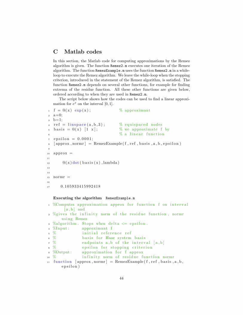
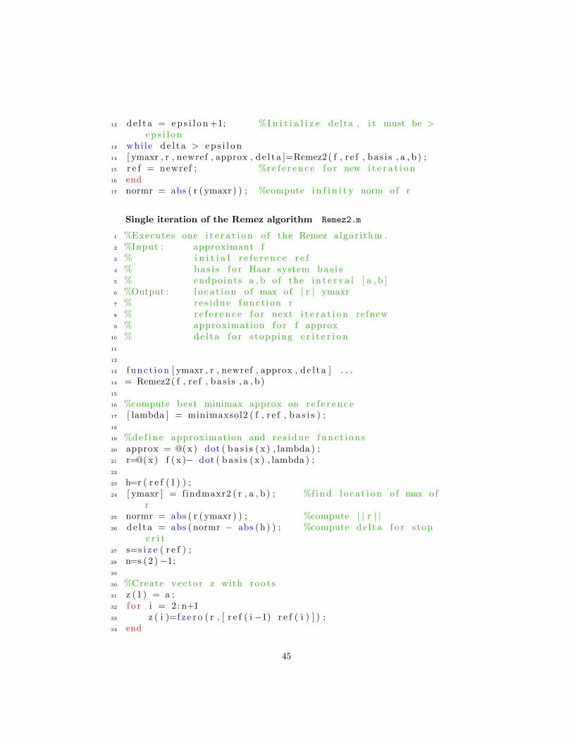
C Matlab codes

In this section, the Matlab code for computing approximations by the Remezalgorithm is given. The function Remez2.m executes one iteration of the Remezalgorithm. The function RemezExample.m uses the function Remez2.m in a while-loop to execute the Remez algorithm. We leave the while-loop when the stoppingcriterion, introduced in the statement of the Remez algorithm, is satisfied. Thefunction Remez2.m depends on several other functions, for example for findingextrema of the residue function. All these other functions are given below,ordered according to when they are used in Remez2.m.

The script below shows how the codes can be used to find a linear approxi-mation for ex on the interval [0, 1].

1 f = @( x ) exp ( x ) ; % approximant2 a=0;3 b=1;4 r e f = l i n s p a c e (a , b , 3 ) ; % equispaced nodes5 b a s i s = @( x ) [ 1 x ] ; % we approximate f by6 % a l i n e a r func t i on7 e p s i l o n = 0 . 0 0 0 1 ;8 [ approx , normr ] = RemezExample ( f , r e f , bas i s , a , b , e p s i l o n )9

10 approx =11

12 @( x ) dot ( b a s i s ( x ) , lambda )13

14

15 normr =16

17 0.105933415992418

Executing the algorithm RemezExample.m

1 %Computes approximation approx f o r func t i on f on i n t e r v a l[ a , b ] and

2 %g i v e s the i n f i n i t y norm o f the r e s i d u e funct ion , normrus ing Remez

3 %algor i thm . Stops when d e l t a <= e p s i l o n .4 %Input : approximant f5 % i n i t i a l r e f e r e n c e r e f6 % b a s i s f o r Haar system b a s i s7 % endpoints a , b o f the i n t e r v a l [ a , b ]8 % e p s i l o n f o r stopping c r i t e r i o n9 %Output : approximation f o r f approx

10 % i n f i n i t y norm of r e s i d u e func t i on normr11 f unc t i on [ approx , normr ] = RemezExample ( f , r e f , bas i s , a , b ,

e p s i l o n )

44

12 d e l t a = e p s i l o n +1; %I n i t i a l i z e de l ta , i t must be >e p s i l o n

13 whi le d e l t a > e p s i l o n14 [ ymaxr , r , newref , approx , d e l t a ]=Remez2 ( f , r e f , bas i s , a , b ) ;15 r e f = newref ; %r e f e r e n c e f o r new i t e r a t i o n16 end17 normr = abs ( r ( ymaxr ) ) ; %compute i n f i n i t y norm o f r

Single iteration of the Remez algorithm Remez2.m

1 %Executes one i t e r a t i o n o f the Remez a lgor i thm .2 %Input : approximant f3 % i n i t i a l r e f e r e n c e r e f4 % b a s i s f o r Haar system b a s i s5 % endpoints a , b o f the i n t e r v a l [ a , b ]6 %Output : l o c a t i o n o f max o f | r | ymaxr7 % r e s i d u e func t i on r8 % r e f e r e n c e f o r next i t e r a t i o n refnew9 % approximation f o r f approx

10 % d e l t a f o r stopping c r i t e r i o n11

12

13 f unc t i on [ ymaxr , r , newref , approx , d e l t a ] . . .14 = Remez2( f , r e f , bas i s , a , b )15

16 %compute bes t minimax approx on r e f e r e n c e17 [ lambda ] = minimaxsol2 ( f , r e f , b a s i s ) ;18

19 %d e f i n e approximation and r e s i d u e f u n c t i o n s20 approx = @( x ) dot ( b a s i s ( x ) , lambda ) ;21 r=@( x ) f ( x )− dot ( b a s i s ( x ) , lambda ) ;22

23 h=r ( r e f (1 ) ) ;24 [ ymaxr ] = findmaxr2 ( r , a , b ) ; %f i n d l o c a t i o n o f max o f

r25 normr = abs ( r ( ymaxr ) ) ; %compute | | r | |26 d e l t a = abs ( normr − abs (h) ) ; %compute d e l t a f o r stop

c r i t27 s=s i z e ( r e f ) ;28 n=s (2 )−1;29

30 %Create vec to r z with roo t s31 z (1 ) = a ;32 f o r i = 2 : n+133 z ( i )=f z e r o ( r , [ r e f ( i −1) r e f ( i ) ] ) ;34 end

45

35 z (n+2)=b ;36

37 f o r i = 1 : n+1 %c r e a t e t r i a l s e t {y 0, . . . , y n}

38 sigma = s ign ( r ( r e f ( i ) ) ) ;39 newref ( i ) = fmaxsigmar ( sigma , r , z ( i ) , z ( i +1) , r e f ( i ) , a ,

b ) ;40 end41

42 i f a<=ymaxr && ymaxr<newref (1 ) %i n s e r t i n g ymaxrin to the r e f e r e n c e

43 i f s i gn ( r ( ymaxr ) ) == s ign ( r ( newref (1 ) ) )44 newref (1 )=ymaxr ;45 e l s e46 f o r i = n+1:−1:247 newref ( i )=newref ( i −1) ;48 end49 newref (1 )=ymaxr ;50 end51 e l s e i f newref (n+1)<=ymaxr && ymaxr<=b52 i f s i gn ( r ( ymaxr ) ) == s ign ( r ( newref (n+1) ) )53 newref (n+1) = ymaxr ;54 e l s e55 f o r i = 1 : n56 newref ( i )=newref ( i +1) ;57 end58 newref (n+1)=ymaxr ;59 end60 e l s e61 f o r i = 2 : n+162 i f newref ( i −1)<=ymaxr && ymaxr<newref ( i )63 i f s i gn ( r ( ymaxr ) ) == s ign ( r ( newref ( i −1) ) )64 newref ( i −1) = ymaxr ;65 e l s e i f s i gn ( r ( ymaxr ) )== s ign ( r ( newref ( i ) ) )66 newref ( i ) = ymaxr ;67 end68 end69 end70 end71 end

Solving linear system to obtain best approximation on a referenceminimaxsol2.m

1 %Solve s l i n e a r system to obta in bes t approximation onr e f e r e n c e r e f

46

2 f unc t i on [ lambda ] = minimaxsol2 ( f , r e f , b a s i s )3 s=s i z e ( r e f ) ;4 n=s (2 )−1;5

6 %Construct r i g h t hand s i d e vec to r7 f o r i = 2 : ( n+1)8 b( i −1)=f ( r e f ( i ) )−power (−1 , i −1)∗ f ( r e f ( 1 ) ) ;9 end

10

11 %Construct matrix A12 vector2=b a s i s ( r e f (1 ) ) ;13 f o r i =1:n14 vector1=b a s i s ( r e f ( i +1) ) ;15 f o r j =1:n16 A( i , j )=vector1 ( j )−power (−1 , i ) ∗ vector2 ( j ) ;17 end18 end19 b=transpose (b) ;20 %Solve Ax=b21 lambda = A\b ;

Brute-force search for absolute maximum of residue function findmaxr2.m

1 %Brute f o r c e search f o r x−coord inate o f maximum of r2 f unc t i on [ ymaxr ] = findmaxr2 ( r , a , b )3 s t e p s i z e = (b−a ) /10000;4

5 %Create vec to r with func t i on va lues6 f o r i =1:100017 v a l v e c t o r ( i ) = abs ( r ( a+s t e p s i z e ∗( i −1) ) ) ;8 end9

10 %Find l o c a t i o n o f l a r g e s t va lue11 maxval = max( v a l v e c t o r ) ;12 f o r i =1:1000113 i f v a l v e c t o r ( i ) == maxval14 ymaxr = a+s t e p s i z e ∗( i −1) ;15 end16 end17 end

Finding local maxima fmaxsigmar.m

1 %Finds d e s i r e d l o c a l maxima o f sigma∗ r2 f unc t i on [ maxsol ] = fmaxsigmar ( sigma , r , lb , ub , xi , a , b )3 f = @( x ) −1∗sigma∗ r ( x ) ;

47

4 maxsol = fminbnd ( f , lb , ub ) ;5

6 %In case a l o c a l maximum was found with sigma∗ r ( x i )>sigma∗ r ( y i )

7 %we s t a r t a brute f o r c e search f o r a d e s i r e d maximum8 i f sigma∗ r ( x i )>sigma∗ r ( maxsol )9 s t e p s i z e = (ub−lb ) /10000;

10 f o r i =1:1000111 v a l v e c t o r ( i ) = sigma∗ r ( lb+s t e p s i z e ∗( i −1) ) ;12 end13 maxval = max( v a l v e c t o r ) ;14 f o r i =1:1000115 i f v a l v e c t o r ( i ) == maxval16 maxsol = lb+s t e p s i z e ∗( i −1) ;17 end18 end19 end20

21 %In case sigma∗ r ( x i ) was a l r eady maximal22 i f sigma∗ r ( x i )>sigma∗ r ( maxsol )23 maxsol=x i ;24 end25

26 %Test va lue s at endpoints o f [ a , b ]27 i f lb == a && sigma∗ r ( a )>sigma∗ r ( maxsol )28 maxsol=a ;29 end30 i f ub == b && sigma∗ r (b)>sigma∗ r ( maxsol )31 maxsol=b ;32 end33 end

48

References

[1] M.J.D. Powell. Approximation theory and methods. Cambridge UniversityPress, United States of America, 1981.

[2] E.W. Cheney. Approximation Theory. Chelsea Publishing Company,United States of America, second edition, 1982.

[3] N.L. Carothers. A Short Course on Approximation Theory. Bowling GreenState University, 2009. Available online.

[4] H.S.V. de Snoo and A.E. Sterk. Functional Analysis An Introduction,January 2017.

[5] R. Pachon and L.N. Trefethen. Barycentric-Remez algorithms for bestpolynomial approximation in the chebfun system. L.N. Bit Numer Math,49:721–741, 2009.

[6] H. Van de Vel. Haar intervals for trigonometric polynomials. Journal ofComputational and Applied Mathematics, 5(4):265–267, 1979.

[7] C.B. Dunham. Families satisfying the Haar condition. Journal of Approx-imation Theory, 12:291–298, 1974.

[8] J.T. Lewis. Restricted Range Approximation and Its Application to DigitalFilter Design. Mathematics of Computation, 29(130):522–539, April 1975.

[9] R.A. DeVore and G.G. Lorentz. Constructive Approximation. Grundlehrender mathematischen Wissenschaften. Springer-Verlag Berlin Heidelberg,United States of America, 1993.

[10] J. Berrut and L.N. Trefethen. Barycentric Lagrange Interpolation. Societyfor Industrial and Applied mathematics, 46(3):501–517, 2004.

[11] H.H. Denman. Minimax Polynomial Approximation. Mathematics of Com-putation, 20(94):257–265, 1966.

[12] S.J. Leon. Linear Algebra with Applications. Pearson Education Limited,United States of America, eighth edition, 2014.

[13] S. Abbott. Understanding Analysis. Springer Science+Business Media,Inc., United States of America, 2001.

49