Finding equilibrium probabilities of QBD processes by spectral methods when eigenvalues vanish

Linear Algebra and its Applications 386 (2004) 207–223www.elsevier.com/locate/laa

Finding equilibrium probabilities of QBDprocesses by spectral methods when eigenvalues

vanishWinfried K. Grassmann∗

Department of Computer Science, University of Saskatchewan, 57 Campus Drive, Engineering Building,Saskatoon, Canada SK S7N 5A9

Received 12 August 2003; accepted 7 December 2003

Submitted by D. Szyld

Abstract

In this paper, we discuss the use of spectral or eigenvalue methods for finding the equi-librium probabilities of quasi-birth–death processes for the case where some eigenvalues arezero. Since this leads to multiple eigenvalues at zero, a difficult problem to analyze, we suggestto eliminate such eigenvalues. To accomplish this, the dimension of the largest Jordan blockmust be established, and some initial equations must be eliminated. The method is demon-strated by two examples, one dealing with a tandem queue, the other one with a shorter queueproblem.© 2004 Elsevier Inc. All rights reserved.

Keywords: Quasi-birth–death process; Tandem queues; Shorter queue; Markov chains; Eigenvalues

1. Introduction

In this paper, we deal with continuous-time Markov chains having the followingblock-structured matrices

∗ Tel.: +1-306-966-4898; fax: +1-306-966-4884.E-mail address: [email protected] (W.K. Grassmann).

0024-3795/$ - see front matter � 2004 Elsevier Inc. All rights reserved.doi:10.1016/j.laa.2003.12.013

208 W.K. Grassmann / Linear Algebra and its Applications 386 (2004) 207–223

Q =

Ab,b Ab,0 0 · · ·A0,b A0,0 A0 0

. . .

0 A2 A1 A0. . .

0. . .

. . .. . .

. (1)

Markov chains of this type are known as quasi-birth–death processes, or QBD pro-cesses. The Markov chain contains the levels b, 0, 1, 2, . . ., and the transition matrixis partitioned according to levels. Each level contains a number of phases. Level b

is the boundary level, and it contains Nb, phases. All other levels contain N phases.The block Ab,b reflects transitions occurring from a state to level b to a state of thesame level, the block Ab,0 contains the rates of going from level b to level 0, andthe block A0,b contains the rates of going from level 0 to b. The block A0,0 mustbe understood in a similar fashion. The blocks Aj contain the rates of changing thelevel by 1 − j , j = 0, 1, 2. A0,0 and all Aj are square matrices of dimension N .

The objective is to find the equilibrium probabilities of the process. Hence, let πn

be the vector of all equilibrium probabilities of level n, n = b, 0, 1, . . .. We assumethat the process is positively recurrent. As pointed out in [6], given a matrix of theform of (1), one can always eliminate πb, the boundary probabilities, obtaining ainfinitesimal generator of the form

Q =

A0,0 A0 0 · · ·A2 A1 A0

. . .

0. . .

. . .. . .

. (2)

Note that A0,0 in (2) is different from A0,0 in (1). To indicate this we replace A0,0 in(1) by A′

0,0, and we determine the A0,0 in (2) as

A0,0 = A′0,0 + A0,b(−Ab,b)

−1Ab,0. (3)

The Ai , i = 0, 1, 2 do not change. As the reader may have guessed, this result canbe obtained by block elimination. As shown by [11], block elimination results ina new Markov chain with all states eliminated censored, which is to say that thesample function while in these states is removed. It follows that the equilibriumprobabilities corresponding to (2) are proportional to the ones corresponding to (1).Hence, without loss of generality, we can assume that the matrix in question has beenbrought into the form given by (2). The equilibrium equations can now be written as:

0 = π0A0,0 + π1A2, (4)

0 = πnA0 + πn+1A1 + πn+2A2, n � 0. (5)

Moreover, if e is the column vector with all its entries equal to 1, we have∞∑

n=0

πne = 1. (6)

W.K. Grassmann / Linear Algebra and its Applications 386 (2004) 207–223 209

According to Neuts [14], the probabilities πn are given by

πn = π0Rn, (7)

where R is the minimal non-negative matrix satisfying

0 = A0 + RA1 + R2A2. (8)

It can be shown that all eigenvalues of R are inside the unit circle.Our focus is on the method of spectral analysis, or eigenvalue method. In this

method, one finds values xi (the eigenvalues), and vectors d(i) /= 0 (the eigenvectors)that satisfy the following equation (see [7,9,12] and references in these papers)

0 = d(i)(A0 + A1xi + A2x2i ) = d(i)A(xi),

where A(x) = A0 + A1x + A2x2. One then forms the diagonal matrix � = diag(xi)

and the matrix D = [d(i)]T. Hence, row i of D is equal to d(i). If all eigenvalues aredistinct, then one has

πn = c�nD. (9)

The vector c can be obtained from (4), (6) and (9) as follows (see also [9]). Eqs. (4)and (9) yield

0 = π0A0,0 + π1A0 = cDA0,0 + c�DA0

or

0 = c(DA0,0 + �DA0). (10)

Eqs. (6) and (9) yield

1 = c diag(1/(1 − xi))De. (11)

Many researchers claim that eigenvalue methods lead to numerical instabilities,and that these instabilities are magnified if there are multiple eigenvalues. The eigen-value x = 0 frequently has a multiplicity greater than 1. However, this paper showshow the resulting numerical difficulties can be bypassed. The mathematical diffi-culty of our method should not be minimized, but compared to a rigorous treatmentof multiple eigenvalues and the corresponding Jordan chains (see e.g. in [4]), ourderivation is relatively straightforward.

Generally, it has been our experience that eigenvalue solutions do not normallylead to numerical difficulties (see [6]). Moreover, we will show that for the methodsdiscussed in this paper, potential problems are easily recognizable by consideringthe components of the vector c, we call them ci . In fact, inaccuracies can only occurwhen some ci are extremely large.

Eigenvalue methods seem to have an edge over matrix analytic methods regardingthe computational complexity. For instance, numerical investigations done by Hav-erkort and Ost [10] and by Mitrani and Chakka [12] indicate that the solution timeswhen using eigenvalue methods are substantially shorter than the ones needed formatrix analytic solutions. Moreover, we recently showed [5, 7] that if the matrices


A0, A1 and A2 are all tridiagonal, eigenvalue methods have a lower time-complexitythan matrix analytic methods. Eigenvalue methods can also help one to discoveranalytical solutions as indicated in [9].

The outline of this paper is as follows: we first discuss the geometric and algebraicmultiplicity of the eigenvalues of R and A(x), together with their Jordan blocks.These concepts are then used to deal with the initial conditions. The theory is thenapplied to solve two examples, one dealing with a tandem queue, the other one deal-ing with the a shorter queue model. Questions of numerical accuracy and computa-tional complexity are then addressed. The last section presents some conclusions.

2. The eigenvalues of R and A(x) and their multiplicity

The eigenvalues of A(x) are, by definition, the roots of the polynomial det A(x).The eigenvalues of R, on the other hand, are the roots of the polynomial det(R − Ix).These definitions reflect the general practice, according to which the definition of aneigenvalue is different, depending whether one deals with a matrix polynomial or amatrix.

We now show that the eigenvalues of the matrix R defined by (8) coincide withthe eigenvalues of A(x) that are inside the unit circle. To prove this, we need thefollowing result:

Theorem 1. There is an invertible matrix Y and a stochastic matrix G such that

A(x) = A0 + A1x + A2x2 = (R − Ix)Y (Gx − I ). (12)

For the proof of this theorem, see [13].We have to distinguish between geometric and arithmetic multiplicity. The geo-

metric multiplicity of an eigenvalue xi is the number of independent eigenvectorsconnected with xi . We denote this number by m(xi). Hence, if DA(xi) = 0, whereD is a rectangular matrix of rank r , and there is no matrix of rank exceeding r , thenm(xi) = r . The algebraic multiplicity of the eigenvalue xi , m(xi), is the multiplicityof the root xi of the polynomial det A(x). The algebraic multiplicity can exceed thegeometric multiplicity.

Theorem 2. All eigenvalues of A(x) inside the unit circle are eigenvalues of R,

and they have the same arithmetic multiplicity. Similarly, all eigenvalues of A(x) onor outside the unit circle are the reciprocals of the eigenvalues of G. Conversely, ifxi is an eigenvalue of R, then xi is an eigenvalue of A(x), and if yi is a non-zeroeigenvalue of G, 1/yi is an eigenvalue of A(x).

Proof. Take the determinant of both sides of (12) to find

det A(x) = det(R − Ix) det Y det(Gx − I ).


Clearly, if xi /= 0 is an eigenvalue of Gx − I , then 1/xi must be an eigenvalue ofG. Also, the eigenvalues of R are strictly inside the unit circle, and since G is astochastic matrix, its eigenvalues must be on or inside the unit circle. If xi = 0, thenit clearly must be an eigenvalue of R, because det(Gx − I ) is ±1 in this case. Ifxi /= 0, and |xi | < 1, it must be an eigenvalue of R, because 1/xi is outside the unitcircle and therefore cannot be an eigenvalue of G. Similarly, if xi is outside the unitcircle, it cannot be an eigenvalue of R, and must therefore be an eigenvalue of G.Hence, R − Ix and Gx − I cannot satisfy the same eigenvalue. It follows that thealgebraic multiplicity m(xi), |xi | < 1, must be the same for R and A(x). �

Theorem 3. The geometric multiplicity of the eigenvalue xi, |xi | < 1 of A(x) isequal to the geometric multiplicity of xi of R.

Proof. If xi is an eigenvalue of A(x) with a geometric multiplicity of m(xi), thenthere is a matrix D with rank m(xi), and no matrix with rank greater m(xi) satisfyingDA(xi) = 0, and, since det(Gxi − I ) /= 0 and det Y /= 0, D(R − Ixi) = 0, and theresult follows. �

0 is an eigenvalue of A(x) if 0 = dA(0) = dA0 has a non-zero solution vectord , that is, A0 must be singular. The geometric multiplicity m(0) of the eigenvaluex = 0 is given by the dimension of the null-space of A0. By Theorem 3, m(0) isalso the geometric multiplicity of the eigenvalue x = 0 of R, or the dimension of thenull-space of R.

The matrix R, like every other matrix, can be factored as

R = D−1�D, (13)

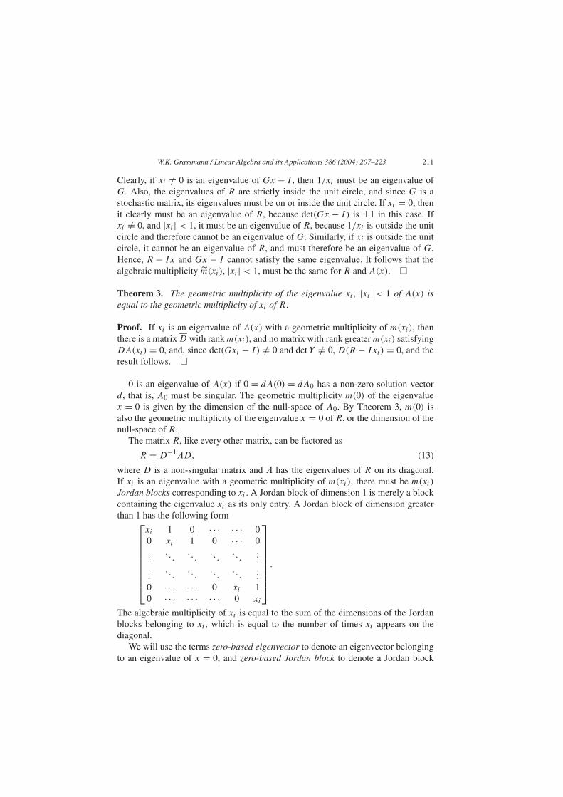
where D is a non-singular matrix and � has the eigenvalues of R on its diagonal.If xi is an eigenvalue with a geometric multiplicity of m(xi), there must be m(xi)

Jordan blocks corresponding to xi . A Jordan block of dimension 1 is merely a blockcontaining the eigenvalue xi as its only entry. A Jordan block of dimension greaterthan 1 has the following form

xi 1 0 · · · · · · 00 xi 1 0 · · · 0...

. . .. . .

. . .. . .

......

. . .. . .

. . .. . .

...

0 · · · · · · 0 xi 10 · · · · · · · · · 0 xi

.

The algebraic multiplicity of xi is equal to the sum of the dimensions of the Jordanblocks belonging to xi , which is equal to the number of times xi appears on thediagonal.

We will use the terms zero-based eigenvector to denote an eigenvector belongingto an eigenvalue of x = 0, and zero-based Jordan block to denote a Jordan block


with 0 on the diagonal. If J is a zero-based Jordan block of dimension d , then J n = 0n � d as is easily verified. Hence, if κ is the size of the largest zero-based Jordanblock, then all zero-based Jordan blocks in Rn = D−1�nD, n � κ , become zero. Asa consequence, the null-space of Rn has dimension m(0) for n � κ .

To find κ , we first consider the Jordan-structure of R, and we then connect this tothe Jordan structure of A(x) by means of (12). The factor Y (Gx − I ) in this equationcannot be singular for |x| < 1. Consequently, for |x| < 1, the null-space of A(x) isequal to the null-space of R. Furthermore, because of (13), we have

R − Ix = D−1�D − Ix = D−1(� − Ix)D.

If one is interested in the dimension of the null-space of R, one can ignore the factorsof D and D−1 and concentrate on the matrix �(0)(x) = � − Ix.

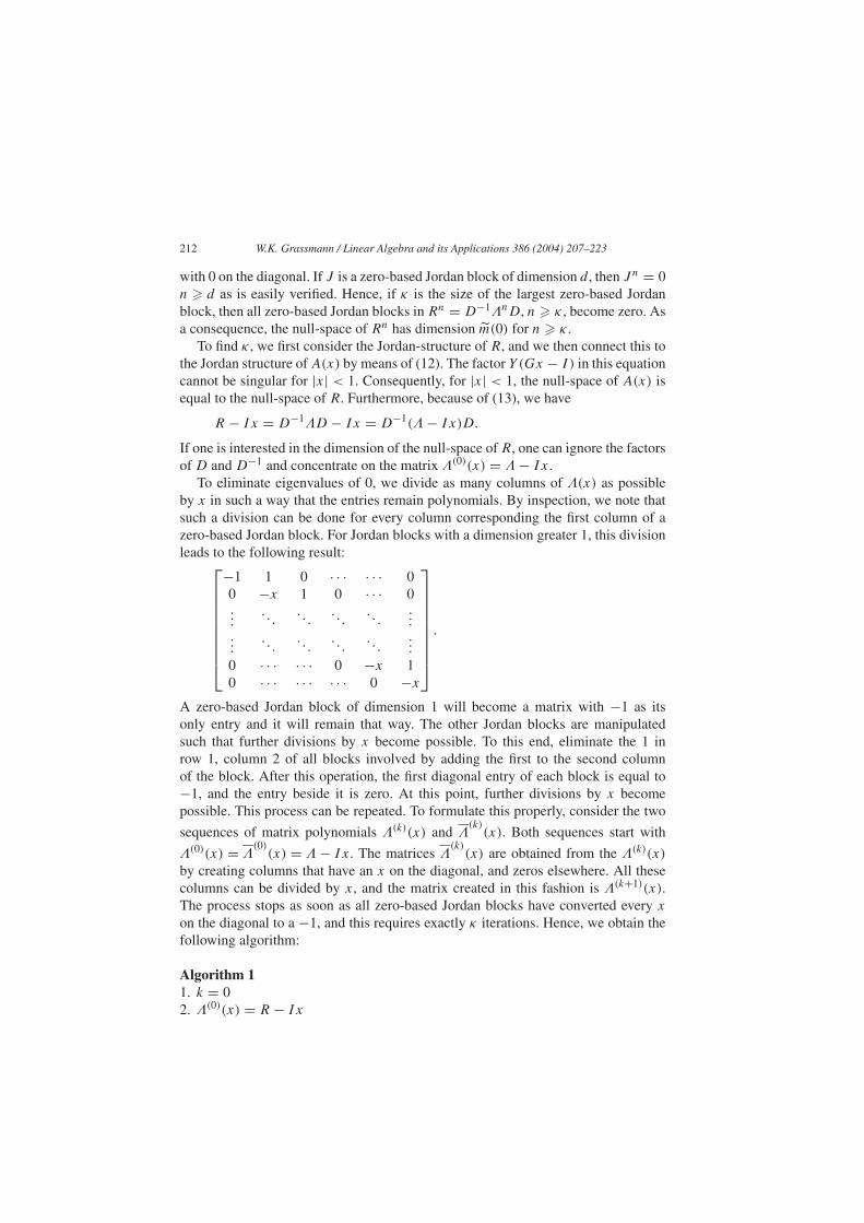
To eliminate eigenvalues of 0, we divide as many columns of �(x) as possibleby x in such a way that the entries remain polynomials. By inspection, we note thatsuch a division can be done for every column corresponding the first column of azero-based Jordan block. For Jordan blocks with a dimension greater 1, this divisionleads to the following result:

−1 1 0 · · · · · · 00 −x 1 0 · · · 0...

. . .. . .

. . .. . .

......

. . .. . .

. . .. . .

...

0 · · · · · · 0 −x 10 · · · · · · · · · 0 −x

.

A zero-based Jordan block of dimension 1 will become a matrix with −1 as itsonly entry and it will remain that way. The other Jordan blocks are manipulatedsuch that further divisions by x become possible. To this end, eliminate the 1 inrow 1, column 2 of all blocks involved by adding the first to the second columnof the block. After this operation, the first diagonal entry of each block is equal to−1, and the entry beside it is zero. At this point, further divisions by x becomepossible. This process can be repeated. To formulate this properly, consider the two

sequences of matrix polynomials �(k)(x) and �(k)

(x). Both sequences start with

�(0)(x) = �(0)

(x) = � − Ix. The matrices �(k)

(x) are obtained from the �(k)(x)

by creating columns that have an x on the diagonal, and zeros elsewhere. All thesecolumns can be divided by x, and the matrix created in this fashion is �(k+1)(x).The process stops as soon as all zero-based Jordan blocks have converted every x

on the diagonal to a −1, and this requires exactly κ iterations. Hence, we obtain thefollowing algorithm:

Algorithm 11. k = 02. �(0)(x) = R − Ix


3. Repeat steps 3.1 through 3.4

3.1 Convert �(k)(x) to �(k)

(x) by creating as many columns as possible with x

as their only entries. Let m(k) the number of columns created this way3.2 If m(k) = 0, exit loop

3.3 Divide each of the m(k) columns of �(k)

(x) having x as its only entry by x tofind �(k+1)(x)

3.4 k = k + 14. κ = k

We modify this algorithm to obtain Algorithm 2, which can be applied to find κ fromA(x).

Algorithm 21. k = 02. A(0)(x) = A(x)

3. Repeat steps 3.1 through 3.43.1 Convert A(k)(x) to A(k)(x) by creating as many columns as possible with

entries that are polynomials with no constant term. Let m(k) the number ofcolumns created this way

3.2 If m(k) = 0, exit loop3.3 Divide each of the m(k) columns of A(k)(x) with no constant term by x to find

A(k+1)(x)

3.4 k = k + 14. κ = k

Algorithm 2 parallels Algorithm 1 it leads to the same value κ .Step 3.1 of Algorithm 2, where polynomial entries with no constant terms are

created, will now be fleshed out in more detail. The constant terms of the polynomialentries are given by the matrix A(k)(0), and we have to create a matrix A(k)(0) thathas the same null-space as A(k)(0), but that has m(k) columns that are 0. This canbe done by adding and subtracting the different columns such that all constants ofthe columns to be divided by x are eliminated. The process essentially creates theechelon form of A(k)(0). As introductory textbooks on linear algebra show (see e.g.[15]), this is equivalent to post-multiplying A(k)(0) with a non-singular matrix, sayB(k). The other steps of the algorithm should be obvious.

The remainder of this section gives additional information about Algorithm 2. Itis more technical, and can be skipped at first reading. We note that whenever wedivide m(k) columns by x, the degree of the polynomial det A(k)(x) is reduced bym(k). It follows that after Algorithm 2, the degree of det A(x) is reduced by m =�κ−1

k=0 m(k−1). Note that any solution (d(i), xi) still satisfies 0 = d(i)A(k)(xi) as longas xi /= 0. To see this, write

A(k+1)(x) = A(k)(x)B(k)I (k)(1/x),


where I (k)(1/x) represents the divisions by x in iteration k. For x /= 0, the matrixI (k)(1/x) is well-defined and non-singular, and if 0 = d(i)A(k)(xi) is a solution, xi /=0, so is

0 = d(i)A(k+1)(xi) = d(i)A(k)(xi)B(k)I (k)(1/xi).

Of course, 0 = d(i)A(xi) = d(i)A(0)(xi), and by induction, 0 = d(i)A(k)(xi) for allvalues of k. Moreover, since A(κ)(0) is not singular, A(κ)(x) has no longer any eigen-value of x = 0. �

3. The elimination of the zero-based eigenvectors

Even in case of multiple eigenvalues, one can still use Eqs. (9), (10) and even (11)provided diag(1/(1 − xi) is replaced by (I − �)−1. However, finding D becomesdifficult for κ > 1, and we therefore use a different method. According to (9), πn =c�nD. For n � κ , the nth power of all zero-based Jordan blocks become 0. To reflectthis, partition � as follows

� =[�0 00 �1

].

Here, �0 is the square matrix containing all zero-based Jordan blocks, and �1 con-tains all other Jordan blocks. Hence,

�n =[

0 00 �n

1

], n � κ.

We partition c and D conformal with � and obtain

πn = [c0 c1][

0 00 �n

1

] [D0D1

]= c1�

n1D1, n � κ.

Hence, c0 and D0 are not needed to find πn, n � κ . Moreover, if n < κ , one canfind πn directly. First, one eliminates all πn, n < κ from the equilibrium equations.Using the GTH algorithm [8], this be done in a numerically stable way. The elimina-tion then provides equations for the backsubstitution step, and hence expressions toevaluate the πn, n < κ . After eliminating πn, n < κ , from the equilibrium equations,we obtain the following matrix

Q(κ) =

Aκ,κ A0 0 · · ·A2 A1 A0

. . .

0. . .

. . .. . .

. (14)

From this system, we find

0 = πκAκ,κ + πκ+1A2.


Since πn = c1�n1D1, n � κ , this yields

0 = c1�κ1(D1Aκ,κ + �1D1A2).

We set c = c1�κ , yielding

0 = c(D1Aκ,κ + �1D1A2). (15)

In addition, the probabilities must be normed such that their sum is 1. This yields N

independent equations for the N − m(0) variables, that is, the system is overdeter-mined.

However, since (10) has a solution, a solution must exist here as well, and thisimplies that the equations are dependent. One can thus choose a subset of theseequations or, alternatively, one can use the least square method. Of course, once c isfound,

πn = c�n−κ1 D1, n � κ. (16)

At this stage, we can summarize the procedure as follows

Algorithm 31. Find all non-zero eigenvalues and the corresponding eigenvectors2. Find D1, the matrix consisting of the non zero-based eigenvectors3. Find κ

4. Eliminate πn, n < κ from the equilibrium equations. This provides expression forπn, n < κ in terms of πn+1, and it also provides Aκ,κ

5. Solve (15) for c, up to a factor f . This factor must later be found by using thecondition that the sum of all probabilities equals 1

6. Use (16) to determine πκ up to a factor f

7. Find πn, n < κ , up to a factor f , by using the equations obtained in step 4 of thisprocedure

8. Find f by using 1 = ∑κ−1n=0 πn + c(I − �)−1D1.

This algorithm provides πn, n � 0, without using any zero-based eigenvector. Hence,the problem of the multiplicity of the eigenvector x = 0 is bypassed.

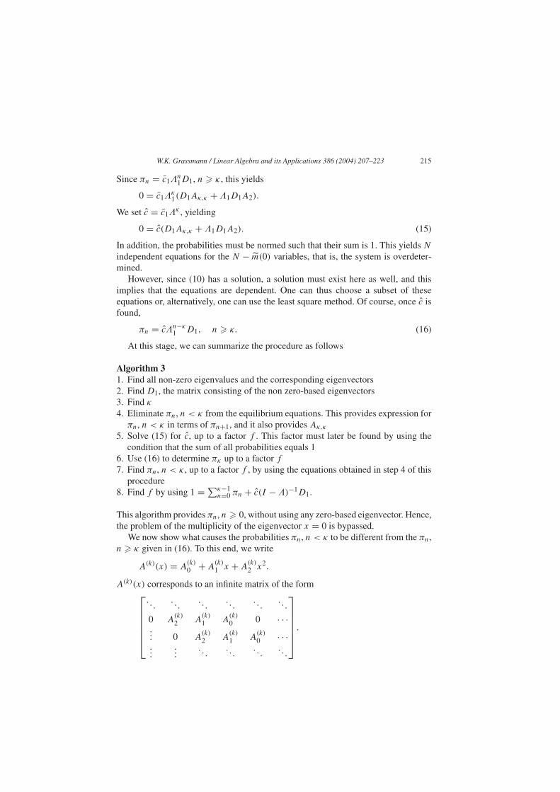
We now show what causes the probabilities πn, n < κ to be different from the πn,n � κ given in (16). To this end, we write

A(k)(x) = A(k)0 + A

(k)1 x + A

(k)2 x2.

A(k)(x) corresponds to an infinite matrix of the form

. . .. . .

. . .. . .

. . .. . .

0 A(k)2 A

(k)1 A

(k)0 0 · · ·

... 0 A(k)2 A

(k)1 A

(k)0 · · ·

......

. . .. . .

. . .. . .

.


To find A(k)(x), columns of this matrix are added or subtracted. This addition orsubtraction is done for all levels, but we never add columns from different levels. Tofind A(k+1)(x) from A(k)(x), some columns are divided by x. A division of a columnby x is equivalent to moving the column up one level as the reader may verify.Instead of moving up one level, one can also take the corresponding column fromthe previous level, and insure in this fashion that we use only the existing columns.Hence, as we go from A(k)(x) to A(k+1)(x), we borrow, so to say, from the previouslevel.

Consider now Q as given in (2). As in Algorithm 2, κ is the first matrix A(k)(x)

non-singular. Since level 0 is different, we are not allowed to borrow from level 0.A(κ) at level n borrows from n − κ and this implies that n must be greater κ in orderto avoid borrowing from level 0. On the other hand, the operations of finding Aκ(x)

do not change the solution πn: we only re-ordered and added equations. It followsthat for level n > κ , we have

0 = πn−1A(κ)0 + πnA

(κ)1 + πn+1A

(κ)2 . (17)

This can now be used for an alternative proof of (16). Since A(κ)(x) has all theeigenvalues and eigenvectors of A(x) except the ones connected with x = 0, A(κ)(x)

shares �1 and D1 with A(x). It follows that πn = c�n−κ1 D1 for high enough n, and

the only thing missing is the value of the first n satisfying this equation. Since A(κ)0

is non-singular, πn−1 is uniquely determined by (17) given πn and πn+1, that is,if n > κ , we have πn−1 = c�n−1−κ

1 D1 as long as πn and πn+1 satisfy a similar for-mula. Hence, the first time πn−1 could be different is when n − 1 < κ , in accordancewith (16).

4. Example 1: A tandem queue

We now apply our theory to solve two examples, in this section a tandem queuemodel, and in the next section a shorter queue model. The tandem queue consideredhere has two stations, both with a single exponential server. Arrivals are Poisson, andthey always join the line of the first server. This line is restricted to N − 1, and oncethe line is full, customers are lost. Customers having received service by the firstserver move on to a second line that has an unlimited capacity to wait for service bythe second server. After having received service by the second server, they leave thesystem. In this model, the second line has to be considered the level, and the firstone as the phase. The rates and the description of the different events affecting thistandem queue is given in Table 1. This table contains all possible events, togetherwith the possible effects on level and phase. It also indicates which matrix Ai isaffected by the event. For instance, an arrival increases line 1 (the phase) by 1, leavingline 2 unchanged. The arrival rate is λ, and this event can only take place if the lengthof the first line is less than N − 1. Arrivals contribute to the matrix A1.


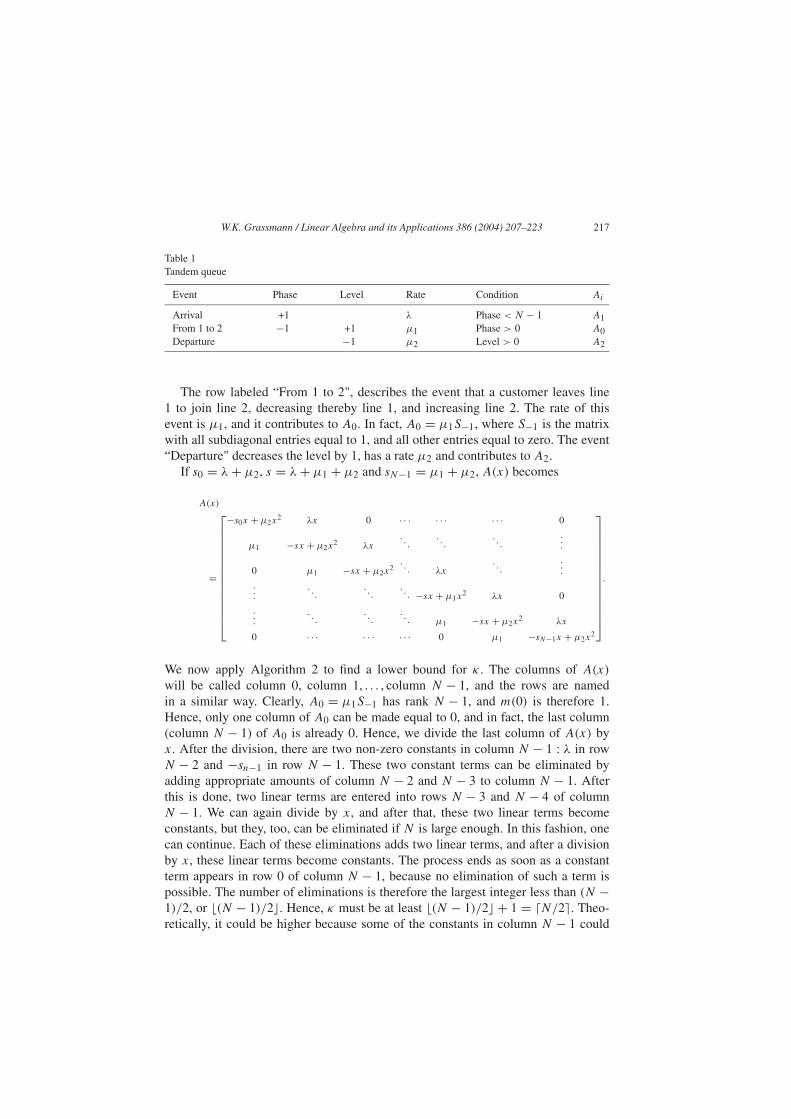
Table 1Tandem queue

Event Phase Level Rate Condition Ai

Arrival +1 λ Phase < N − 1 A1From 1 to 2 −1 +1 µ1 Phase > 0 A0Departure −1 µ2 Level > 0 A2

The row labeled “From 1 to 2", describes the event that a customer leaves line1 to join line 2, decreasing thereby line 1, and increasing line 2. The rate of thisevent is µ1, and it contributes to A0. In fact, A0 = µ1S−1, where S−1 is the matrixwith all subdiagonal entries equal to 1, and all other entries equal to zero. The event“Departure" decreases the level by 1, has a rate µ2 and contributes to A2.

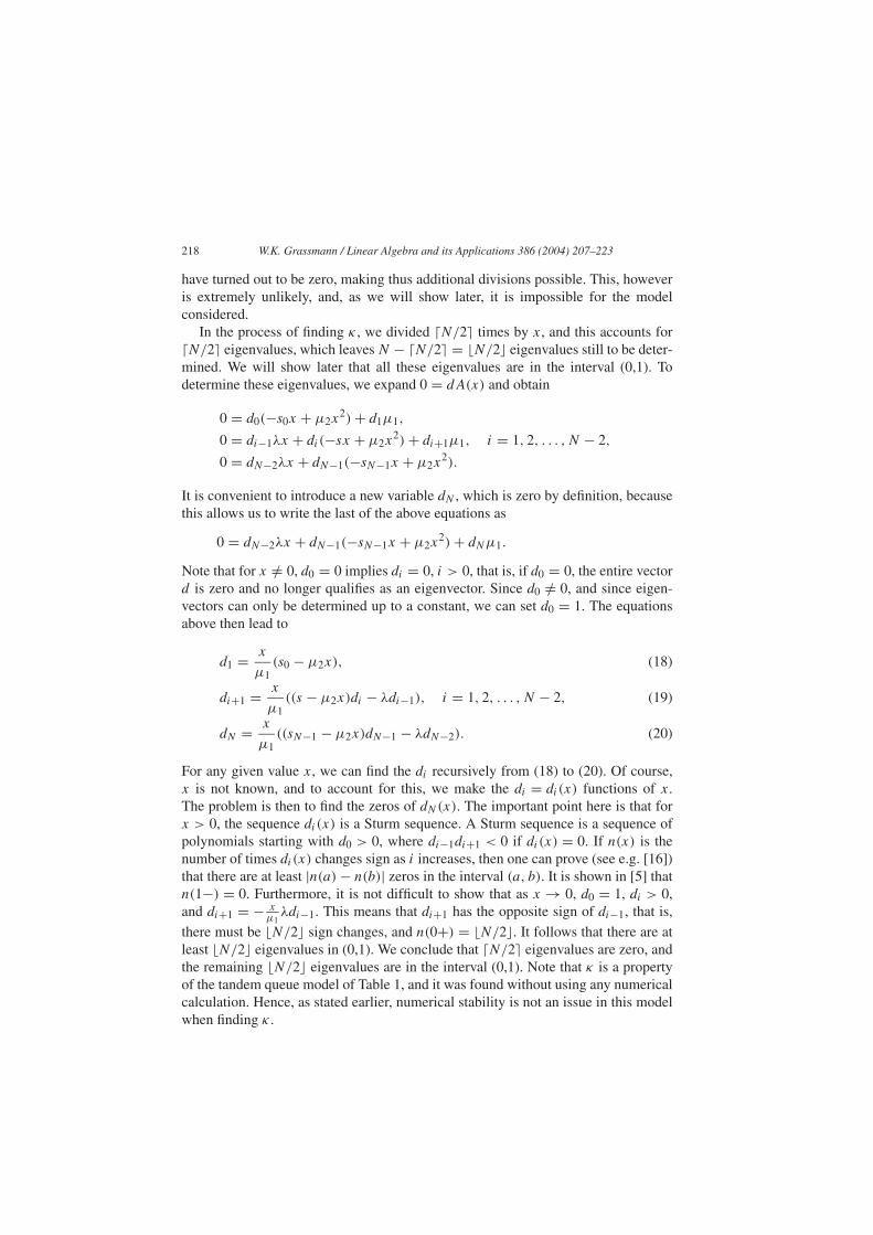
If s0 = λ + µ2, s = λ + µ1 + µ2 and sN−1 = µ1 + µ2, A(x) becomes

A(x)

=

−s0x + µ2x2 λx 0 · · · · · · · · · 0

µ1 −sx + µ2x2 λx

. . .. . .

. . ....

0 µ1 −sx + µ2x2

. . . λx. . .

.

.

.

.

.

.. . .

. . .. . . −sx + µ1x

2 λx 0

.

.

.. . .

. . .. . . µ1 −sx + µ2x

2 λx

0 · · · · · · · · · 0 µ1 −sN−1x + µ2x2

.

We now apply Algorithm 2 to find a lower bound for κ . The columns of A(x)

will be called column 0, column 1, . . . , column N − 1, and the rows are namedin a similar way. Clearly, A0 = µ1S−1 has rank N − 1, and m(0) is therefore 1.Hence, only one column of A0 can be made equal to 0, and in fact, the last column(column N − 1) of A0 is already 0. Hence, we divide the last column of A(x) byx. After the division, there are two non-zero constants in column N − 1 : λ in rowN − 2 and −sn−1 in row N − 1. These two constant terms can be eliminated byadding appropriate amounts of column N − 2 and N − 3 to column N − 1. Afterthis is done, two linear terms are entered into rows N − 3 and N − 4 of columnN − 1. We can again divide by x, and after that, these two linear terms becomeconstants, but they, too, can be eliminated if N is large enough. In this fashion, onecan continue. Each of these eliminations adds two linear terms, and after a divisionby x, these linear terms become constants. The process ends as soon as a constantterm appears in row 0 of column N − 1, because no elimination of such a term ispossible. The number of eliminations is therefore the largest integer less than (N −1)/2, or �(N − 1)/2�. Hence, κ must be at least �(N − 1)/2� + 1 = �N/2�. Theo-retically, it could be higher because some of the constants in column N − 1 could


have turned out to be zero, making thus additional divisions possible. This, howeveris extremely unlikely, and, as we will show later, it is impossible for the modelconsidered.

In the process of finding κ , we divided �N/2� times by x, and this accounts for�N/2� eigenvalues, which leaves N − �N/2� = �N/2� eigenvalues still to be deter-mined. We will show later that all these eigenvalues are in the interval (0,1). Todetermine these eigenvalues, we expand 0 = dA(x) and obtain

0 = d0(−s0x + µ2x2) + d1µ1,

0 = di−1λx + di(−sx + µ2x2) + di+1µ1, i = 1, 2, . . . , N − 2,

0 = dN−2λx + dN−1(−sN−1x + µ2x2).

It is convenient to introduce a new variable dN , which is zero by definition, becausethis allows us to write the last of the above equations as

0 = dN−2λx + dN−1(−sN−1x + µ2x2) + dNµ1.

Note that for x /= 0, d0 = 0 implies di = 0, i > 0, that is, if d0 = 0, the entire vectord is zero and no longer qualifies as an eigenvector. Since d0 /= 0, and since eigen-vectors can only be determined up to a constant, we can set d0 = 1. The equationsabove then lead to

d1 = x

µ1(s0 − µ2x), (18)

di+1 = x

µ1((s − µ2x)di − λdi−1), i = 1, 2, . . . , N − 2, (19)

dN = x

µ1((sN−1 − µ2x)dN−1 − λdN−2). (20)

For any given value x, we can find the di recursively from (18) to (20). Of course,x is not known, and to account for this, we make the di = di(x) functions of x.The problem is then to find the zeros of dN(x). The important point here is that forx > 0, the sequence di(x) is a Sturm sequence. A Sturm sequence is a sequence ofpolynomials starting with d0 > 0, where di−1di+1 < 0 if di(x) = 0. If n(x) is thenumber of times di(x) changes sign as i increases, then one can prove (see e.g. [16])that there are at least |n(a) − n(b)| zeros in the interval (a, b). It is shown in [5] thatn(1−) = 0. Furthermore, it is not difficult to show that as x → 0, d0 = 1, di > 0,and di+1 = − x

µ1λdi−1. This means that di+1 has the opposite sign of di−1, that is,

there must be �N/2� sign changes, and n(0+) = �N/2�. It follows that there are atleast �N/2� eigenvalues in (0,1). We conclude that �N/2� eigenvalues are zero, andthe remaining �N/2� eigenvalues are in the interval (0,1). Note that κ is a propertyof the tandem queue model of Table 1, and it was found without using any numericalcalculation. Hence, as stated earlier, numerical stability is not an issue in this modelwhen finding κ .


5. Example 2: A shorter queue model

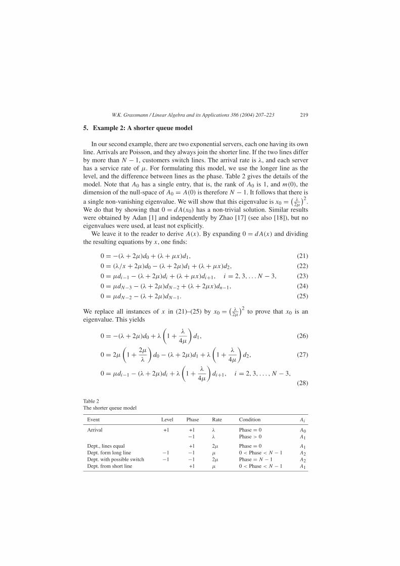
In our second example, there are two exponential servers, each one having its ownline. Arrivals are Poisson, and they always join the shorter line. If the two lines differby more than N − 1, customers switch lines. The arrival rate is λ, and each serverhas a service rate of µ. For formulating this model, we use the longer line as thelevel, and the difference between lines as the phase. Table 2 gives the details of themodel. Note that A0 has a single entry, that is, the rank of A0 is 1, and m(0), thedimension of the null-space of A0 = A(0) is therefore N − 1. It follows that there isa single non-vanishing eigenvalue. We will show that this eigenvalue is x0 = (

λ2µ

)2.We do that by showing that 0 = dA(x0) has a non-trivial solution. Similar resultswere obtained by Adan [1] and independently by Zhao [17] (see also [18]), but noeigenvalues were used, at least not explicitly.

We leave it to the reader to derive A(x). By expanding 0 = dA(x) and dividingthe resulting equations by x, one finds:

0 = −(λ + 2µ)d0 + (λ + µx)d1, (21)

0 = (λ/x + 2µ)d0 − (λ + 2µ)d1 + (λ + µx)d2, (22)

0 = µdi−1 − (λ + 2µ)di + (λ + µx)di+1, i = 2, 3, . . . N − 3, (23)

0 = µdN−3 − (λ + 2µ)dN−2 + (λ + 2µx)dn−1, (24)

0 = µdN−2 − (λ + 2µ)dN−1. (25)

We replace all instances of x in (21)–(25) by x0 = (λ

2µ

)2 to prove that x0 is aneigenvalue. This yields

0 = −(λ + 2µ)d0 + λ

(1 + λ

4µ

)d1, (26)

0 = 2µ

(1 + 2µ

λ

)d0 − (λ + 2µ)d1 + λ

(1 + λ

4µ

)d2, (27)

0 = µdi−1 − (λ + 2µ)di + λ

(1 + λ

4µ

)di+1, i = 2, 3, . . . , N − 3,

(28)

Table 2The shorter queue model

Event Level Phase Rate Condition Ai

Arrival +1 +1 λ Phase = 0 A0−1 λ Phase > 0 A1

Dept., lines equal +1 2µ Phase = 0 A1Dept. form long line −1 −1 µ 0 < Phase < N − 1 A2Dept. with possible switch −1 −1 2µ Phase = N − 1 A2Dept. from short line +1 µ 0 < Phase < N − 1 A1


0 = µdN−3 − (λ + 2µ)dN−2 + λ

(1 + λ

2µ

)dN−1, (29)

0 = µdN−2 − (λ + 2µ)dN−1. (30)

Obviously, (28) is a difference equation, and we can therefore use the trial solutiondi = yi−1, where y must satisfy

0 = µ − (λ + 2µ)y + λ

(1 + λ

4µ

)y2.

One solution of this equation is:

y = 1

2 + λ/(2µ).

We try this solution and set

di = yi−1 = 1

(2 + λ(2µ))i−1, i = 1, 2, . . . , N − 2. (31)

d0 can now be found from (26) and dN−1 from (30):

d0 = λ

(1 + λ

4µ

)/(λ + 2µ), dN−1 = µ

λ + 2µ

(1

2 + λ/(2µ)

)N−3

.

(32)

It is now a simple matter to verify that the solution given by (31) and (32) satisfiesEqs. (27) and (29), that is, the value of y used is the correct one. A similar result wasfound by Adan [1].

The approach based on difference equations discussed can be used for other prob-lems as well, even when the eigenvalues are not known, as shown in [7] or [9]. Wecould even have used it to solve example 1. This would have reduced the computa-tional complexity, but it would have increased the mathematical effort considerably.

Consider now the case where there are more than two lines in parallel. The levelis given by the longest line, and the phase is some kind of enumeration of the differ-ences between the lines. Even in this case, the only way the longer line can increaseis when all lines are of equal length, that is, A0 has only one entry, and there istherefore only one eigenvalue that is not zero. In [18], Zhao even shows, though notby using our concepts, that the number of non-zero eigenvalues remains 1 even if theservers are non-homogeneous, and even if arrivals are not Poisson.

Care must be taken to make sure that the level is chosen such that A0 has a fewentries as possible. For instance, the reader may verify that if the shorter line is usedas the level, A0 = λS−1, and the geometric multiplicity is only 1, but the algebraicmultiplicity is N − 1!

6. Numerical considerations

In this section, we compare our methods with matrix analytic methods in terms ofaccuracy and computational complexity. We restrict our attention to the case where


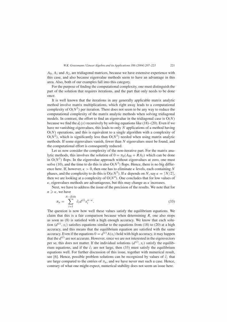
A0, A1 and A2, are tridiagonal matrices, because we have extensive experience withthis case, and also because eigenvalue methods seem to have an advantage in thisarea. Also, both of our examples fall into this category.

For the purpose of finding the computational complexity, one must distinguish thepart of the solution that requires iterations, and the part that only needs to be doneonce.

It is well known that the iterations in any generally applicable matrix analyticmethod involve matrix multiplications, which right away leads to a computationalcomplexity of O(N3) per iteration. There does not seem to be any way to reduce thecomputational complexity of the matrix analytic methods when solving tridiagonalmodels. In contrast, the effort to find an eigenvalue in the tridiagonal case is O(N)

because we find the di(x) recursively by solving equations like (18)–(20). Even if wehave no vanishing eigenvalues, this leads to only N applications of a method havingO(N) operations, and this is equivalent to a single algorithm with a complexity ofO(N2), which is significantly less than O(N3) needed when using matrix analyticmethods. If some eigenvalues vanish, fewer than N eigenvalues must be found, andthe computational effort is consequently reduced.

Let us now consider the complexity of the non-iterative part. For the matrix ana-lytic methods, this involves the solution of 0 = π0(A00 + RA2) which can be donein O(N3) flops. In the eigenvalue approach without eigenvalues at zero, one mustsolve (10), and the time to do this is also O(N3) flops. Hence, there is no big differ-ence here. If, however, κ > 0, then one has to eliminate κ levels, each containing N

phases, and the complexity to do this is O(κN3). If κ depends on N , say κ = �N/2�,then we are looking at a complexity of O(N4). One concludes that for low values ofκ , eigenvalues methods are advantageous, but this may change as κ increases.

Next, we have to address the issue of the precision of the results. We note that forn � κ , we have

πn =N−m(0)∑

i=1

cid(i)xn−κ

i . (33)

The question is now how well these values satisfy the equilibrium equations. Weclaim that this is a fair comparison because when determining R, one also stopsas soon as (8) is satisfied with a high enough accuracy. We know that each solu-tion (d(i), xi) satisfies equations similar to the equations from (18) to (20) at a highaccuracy, and this means that the equilibrium equation are satisfied with the sameaccuracy. Even if the equations 0 = d(i)A(xi) hold with high accuracy, it may happenthat the d(i) are not accurate. However, since we are not interested in the eigenvectorsper se, this does not matter. If the individual solutions (d(i), xi) satisfy the equilib-rium equations, and if the ci are not large, then (33) must satisfy the equilibriumequations well. For further discussion of this issue, together with numerical result,see [6]. Hence, possible problem solutions can be recognized by values of ci thatare large compared to the entries of πn, and we have never met such a case. Hence,contrary of what one might expect, numerical stability does not seem an issue here.


7. Conclusion

Eigenvalues of zero occur whenever A0 is singular, and A0 is singular wheneverafter an increase of the level, some phases cannot be reached. In addition to the exam-ples discussed here, there are many others. For instance, if the level is the numberin any queue that is increased through Erlang-k arrivals, then after an arrival, onlyone phase is possible, which reduces the number of non-vanishing eigenvalues by afactor of k. For further examples of problems with vanishing eigenvalues, see [2,3].

A criticism leveled against the use of eigenvalue methods is that they may involveeigenvalues of multiplicity greater than 1, which is considered harmful. The eigen-value x = 0 often has a multiplicity greater one, but in this particular case, the math-ematical and numerical problems one would expect can be bypassed: One merelyeliminates all eigenvalues x = 0, and obviously, things that are eliminated no longerexist and can therefore do no harm. To do the elimination, one has to find κ , thesize of the largest Jordan block having x = 0 as an eigenvalue. Finding κ is typicallydone for entire classes of models, and it does not involve specific rates, and henceits determination is not a numerical problem, but a mathematical one. In conclusion,this paper has presented tools one can use to defuse the problems caused by multipleeigenvalues at zero.

Acknowledgements

The authors thanks the referees for their valuable suggestions. Contract/grantsponsor: Research supported in part by NSERC Disvovery Grant; contract/grantnumber: 8112.

References

[1] I.J.B.F. Adan, The compensation approach for queueing problems, Ph.D. Thesis, Technische Uni-versiteit Eindhoven, 1991.

[2] A.S. Alfa, Discrete time queues and matrix-analytic methods, TOP 10 (2) (2002) 147–210.[3] A.S. Alfa, Combined elapsed time and matrix-analytic method for the discrete time GI/G/1 and

the GIX/G/1 systems, Queueing Syst. Theory Appl. 45 (2003) 5–25.[4] I. Gohberg, P. Lancaster, L. Rodman, Matrix Polynomials, Academic Press, New York, 1982.[5] W.K. Grassmann, Real eigenvalues of certain tridiagonal matrix polynomials, with queueing appli-

cations, J. Linear Algebra Appl. 342 (2002) 93–106.[6] W.K. Grassmann, The use of eigenvalues for finding equilibrium probabilities of certain Markovian

two-dimensional queueing problems, INFORMS J. Comput. 15 (2003) 412–421.[7] W.K. Grassmann, S. Drekic, An analytical solution for a tandem queue with blocking, Queueing

Syst. 36 (2000) 221–235.[8] W.K. Grassmann, M. Taksar, D.P. Heyman, Regenerative analysis and steady state distributions for

Markov chains, Oper. Res. 33 (1993) 1107–1117.[9] W.K. Grassmann, J. Tavakoli, A tandem queue with a movable server: an eigenvalue approach,

SIAM J. Matrix Anal. Appl. (2002) 465–474.


[10] B.R. Haverkort, A. Ost, Steady-state analysis of infinite stochastic Petri nets: a comparison betweenthe spectral expansion and the matrix-geometric method, in: Proceedings of the 7th InternationalWorkshop on Petri Nets and Performance Models, Saint Malo, France, IEEE Computer SocietyPress, 1997, pp. 36–45.

[11] J.G. Kemeny, J.L. Snell, A.W. Knapp, Denumerable Markov Chains, Van Nostrand, Princeton, NJ,1966.

[12] I. Mitrani, R. Chakka, Spectral expansion solution for a class of Markov models: application andcomparison with the matrix-geometric method, Perform. Evaluat. 23 (1995) 241–260.

[13] V. Naoumov, Matrix-multiplicative approach to quasi-birth-and-death processes analysis, in:Matrix-Analytic Methods in Stochastic Models, Marcel Dekker, New York, 1996, pp. 87–106.

[14] M.F. Neuts, Matrix-Geometric Solutions in Stochastic Models, Johns Hopkins University Press,Baltimore, 1981.

[15] G. Strang, Linear Algebra and Its Applications, second ed., Academic Press, New York, 1980.[16] H.W. Turnbull, Theory of Equations, fifth ed., Oliver and Boyed, Edingurgh, 1952.[17] Y. Zhao, Shortest queue models, Ph.D. Thesis, University of Saskatchewan, 1990.[18] Y. Zhao, W.K. Grassmann, Queueing analysis of the jockeying model, Oper. Res. 43 (1995) 520–

529.

Documents

Finding equilibrium probabilities of QBD processes by spectral methods when eigenvalues vanish