www.elsevier.com/locate/asr

Advances in Space Research 36 (2005) 757–761

Finding SZ clusters in the ACBAR maps

E. Pierpaoli a,*, S. Anthoine b

a California Institute of Technology, MPA, Mail Code 130-33, Pasadena, CA 91125, USAb Department of Applied Mathematics, Princeton University, Princeton, NJ 08544, USA

Received 30 October 2004; received in revised form 8 February 2005; accepted 9 February 2005

Abstract

We present a new method for component separation from multi-frequency maps aimed to extract Sunyaev–Zeldovich (SZ) gal-

axy clusters from cosmic microwave background (CMB) experiments. This method is best suited to recover non-Gaussian, spatially

localized and sparse signals. We apply our method on simulated maps of the ACBAR experiment. We find that this method

improves the reconstruction of the integrated y parameter by a factor of three with respect to the Wiener filter case. Moreover,

the scatter associated with the reconstruction is reduced by 30%.

� 2005 COSPAR. Published by Elsevier Ltd. All rights reserved.

Keywords: Large-scale structure of Universe; Cosmic microwave background; Galaxies: clusters: general

1. Introduction

The study of the cosmic microwave background(CMB) has greatly improved our understanding of

the Universe in the last decade. The measurement

and interpretation of the CMB power spectrum has al-

lowed to determine the most important cosmological

parameters with very high accuracy. More experiments,

now planned or underway, will produce higher resolu-

tion multi-frequency maps of the sky in the 100–

400 GHz frequency range. One of the most importantnew scientific goals of these experiments is the detec-

tion of clusters through their characteristic Sunyaev–

Zeldovich (SZ) signature (Sunyaev and Zeldovich,

1980). Because the SZ signal is substantially indepen-

dent of redshift, SZ clusters will be observed at very

large distances, quite independently from their mass.

Such clusters may be used to infer cosmological infor-

mation via number counts and power spectrum analy-sis of SZ maps. Many studies have shown the great

0273-1177/$30 � 2005 COSPAR. Published by Elsevier Ltd. All rights reser

doi:10.1016/j.asr.2005.02.018

* Corresponding author. Tel.: +1 626 395 4301.

E-mail address: pierpa@caltech.edu (E. Pierpaoli).

potential of these new technique. These estimates, how-

ever, typically assume that all clusters above a certain

flux are perfectly reconstructed and detected in theCMB maps. In practice, this may not be the case. SZ

clusters have radio intensities comparable to other

intervening cosmological signals like the CMB and

point sources. Despite the different frequency and spa-

tial dependence of these signals, it is not so easy to dis-

entangle them. Moreover, beam smearing and

instrumental noise play a role in our ability to ade-

quately reconstruct the observed cluster. These argu-ments raise the necessity to assess how well a certain

technique performs in reconstructing the cluster signal

given the experiment specifications. For a given cluster

Compton parameter y, the reconstructed value may

also depend on the cluster location and shape. There-

fore, there is an error associated with the reconstruc-

tion technique which needs to be assessed and

accounted for when it comes to relate cluster�s observ-ables with cosmological models. Moreover, the specific

observable to use may depend on the type of experi-

ment in hand. In this paper we address these issues

for the ACBAR experiment (see Pierpaoli et al., 2004

ved.

758 E. Pierpaoli, S. Anthoine / Advances in Space Research 36 (2005) 757–761

for a similar analysis applied to Planck and ACT). Sev-

eral techniques have been developed for image recon-

struction in the multi-component case (Herranz et al.,

2002; Stolyarov et al., 2002). In most cases, these tech-

niques are optimal in reconstructing the CMB fluctua-

tion signal, which is Gaussian and well-characterized inFourier space. Clusters of galaxies maps present very

different features from CMB ones, in particular: (i)

clusters are ‘‘rare’’ objects in the map, they do not fill

out the majority of the space; (ii) the cluster signal is

non-Gaussian on several scales, and in particular on

scales associated with the typical core size; (iii) different

scales are correlated in Fourier space. Keeping these

characteristics in mind, in this paper we develop amethod aimed to better reconstruct the SZ galaxy clus-

ter signal from multi-frequency maps. Our map recon-

struction method is wavelet based and is best suited to

reconstruct the specific non-Gaussian signal expected in

galaxy clusters maps. In this work we use the simulated

cluster maps by Martin White available at: http://

pac1.berkeley.edu/tSZ/. These maps are not full hydro-

dynamical simulations, the gas here has been intro-duced using the dark matter as a tracer. However,

for the kind of experiment in hand which would not re-

solve the cluster structure anyway, this should not pres-

ent a major problem. The underlying cosmology

corresponds to the concordance model. We used 10

maps of 10� · 10�.

2. The reconstruction method

2.1. The wavelet decomposition used

We use a two-dimensional overcomplete wavelet rep-

resentation which is more adequate to the analysis of

astrophysical images. The wavelet decomposition of a

signal s in our case reads

s ¼Xq2N2

hs;/qi/q þXJ

j¼0

XMm¼1

Xq22�jN2

hs;wj;m;qiwj;m;q; ð1Þ

where /q are the scaling functions, wj,m, q are the wave-

lets and Æ,æ are scalar products. The sumP

qhs;/qi/q is

the projection of s on the coarsest scale, i.e., a low-pass

version of s. Each scaling coefficient Æs, /qæ contains

information about the signal s at the coarsest scale

and at a specific location in space q. For j fixed, the

sumP

m

Pqhs;wj;m;qiwj;m;q is the projection of s on the

scale j, i.e., a band-pass version of s. Each wavelet coef-

ficient Æs, wj,m, qæ contains information about the signal s

at the specific scale j, orientation m and location in space

q. As usual with wavelet transforms, changing scale is

done by dilating, and changing location is done by

translating the wavelet: wj + 1,m, q(x) = wj,m, q(2x) and

wj,m, q(x) = wj,m, 0(x � q) Hence, scale j + 1 corresponds

to a frequency band that is twice as wide and for which

the central frequencies are twice as large as that of scale

j. On the other hand, in space, the wavelets at scale j + 1

are better localized than at scale j since they are more

narrowly concentrated around their center q (see Fig.

1, column 1 and 2). Unlike the two-dimensional Daube-chies wavelets, the wavelets (and scaling function) we

use here are defined in the Fourier plane. This ensures

that they are well-concentrated in frequency. Moreover,

it enables us to introduce orientation by rotating the

Fourier transform of the wavelet (see Fig. 1, column 2

and 3). If ~f is the Fourier transform of f and (r, h) arepolar coordinates, then: gwj;m;qðr; hÞ ¼ gwj;0;qðr; h� mp

M ÞThe transform is therefore close to rotation invariantand computation is fast via FFT. The Fourier transform

of the wavelets and scaling functions read:

LðrÞ ¼ cosp2log2ðrÞ

� �d1<r<2 þ dr<1 low-pass; ð2Þ

HðrÞ ¼ sinp2log2ðrÞ

� �d1<r<2 þ dr>2 high-pass; ð3Þ

GMðhÞ ¼ðM � 1Þ!ffiffiffiffiffiffiffiffiffiffiffiffiffiffiffiffiffiffiffiffiffiffiffiffiffiffiffiffiM ½2ðM � 1Þ�!

p 2 cos hj jM�1oriented; ð4Þ

f/0ðr; hÞ ¼ Lð2r; hÞ; ð5Þ

gwj;m;0ðr; hÞ ¼ Lr

2j

� �H

2r

2j

� �GM h� mp

M

� �j P 0; 0 6 m < M : ð6Þ

The set of all wavelets and scaling functions deter-

mines a redundant system (they are linearly dependent),

however, the Plancherel equation holds.

2.2. The estimator

Formally, our goal is to estimate several processes

(CMB, SZ, point sources) from their contributions in

observations at different frequencies. We estimate the

processes {x(p, m0)}p from the observations {y(m)}m gi-

ven that: y(m) =P

pf(p, m)x(p, m0) * B(m) + N(m), wherex(p, m0) is the template of the pth process at a given fre-

quency m0, f(p, m) is the frequency dependence of the pth

process, B(m) is the beam and N(m) is the frequency

dependent white noise. Our estimation method will rely

on two principles to discriminate the contributions

from different processes. The first one is that we know

some statistical properties of the processes (e.g., the

CMB and noise are Gaussian processes, while the clus-ters are not). The second one is that some spatial prop-

erties of the processes can be captured by modeling the

coherence of wavelet coefficients. For example, clusters

can be described as spatially localized structures with a

high intensity peak. To estimate a particular wavelet

coefficient xj, m, q, one describes the statistics of a

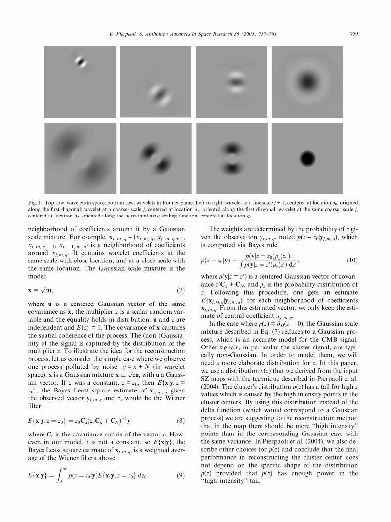
Fig. 1. Top row: wavelets in space; bottom row: wavelets in Fourier plane. Left to right: wavelet at a fine scale j + 1, centered at location q0, oriented

along the first diagonal; wavelet at a coarser scale j, centered at location q1, oriented along the first diagonal; wavelet at the same coarser scale j,

centered at location q2, oriented along the horizontal axis; scaling function, centered at location q2.

E. Pierpaoli, S. Anthoine / Advances in Space Research 36 (2005) 757–761 759

neighborhood of coefficients around it by a Gaussian

scale mixture. For example, xj, m, q = (xj, m, q, xj, m, q + 1,

xj, m, q � 1, xj � 1, m, q) is a neighborhood of coefficients

around xj,m, q. It contains wavelet coefficients at the

same scale with close location, and at a close scale with

the same location. The Gaussian scale mixture is the

model:

x �ffiffiz

pu; ð7Þ

where u is a centered Gaussian vector of the same

covariance as x, the multiplier z is a scalar random var-iable and the equality holds in distribution. u and z are

independent and E{z} = 1. The covariance of x captures

the spatial coherence of the process. The (non-)Gaussia-

nity of the signal is captured by the distribution of the

multiplier z. To illustrate the idea for the reconstruction

process, let us consider the simple case where we observe

one process polluted by noise: y = x + N (in wavelet

space). x is a Gaussian mixture x � ffiffiz

pu, with u a Gauss-

ian vector. If z was a constant, z = z0, then E{x|y, z =

z0}, the Bayes Least square estimate of xj, m, q given

the observed vector yj,m, q and z, would be the Wiener

filter

Efxjy; z ¼ z0g ¼ z0Cxðz0Cx þ CN Þ�1y: ð8Þ

where Cv is the covariance matrix of the vector v. How-

ever, in our model, z is not a constant, so E{x|y}, the

Bayes Least square estimate of xj,m, q, is a weighted aver-

age of the Wiener filters above

Efxjyg ¼Z 1

0

pðz ¼ z0jyÞEfxjy; z ¼ z0g dz0: ð9Þ

The weights are determined by the probability of z gi-

ven the observation yj,m, q, noted p(z = z0|yj,m, q), which

is computed via Bayes rule

pðz ¼ z0jyÞ ¼pðyjz ¼ z0Þpzðz0ÞRpðyjz ¼ z0Þpzðz0Þ dz0

; ð10Þ

where p(y|z = z 0) is a centered Gaussian vector of covari-

ance z 0Cx + CN, and pz is the probability distribution of

z. Following this procedure, one gets an estimate

E{xj,m, q|yj,m, q} for each neighborhood of coefficientsxj,m, q. From this estimated vector, we only keep the esti-

mate of central coefficient xj,m, q.

In the case where p(z) = dD(z � 0), the Gaussian scale

mixture described in Eq. (7) reduces to a Gaussian pro-

cess, which is an accurate model for the CMB signal.

Other signals, in particular the cluster signal, are typi-

cally non-Gaussian. In order to model them, we will

need a more elaborate distribution for z. In this paper,we use a distribution p(z) that we derived from the input

SZ maps with the technique described in Pierpaoli et al.

(2004). The cluster�s distribution p(z) has a tail for high z

values which is caused by the high intensity points in the

cluster centers. By using this distribution instead of the

delta function (which would correspond to a Gaussian

process) we are suggesting to the reconstruction method

that in the map there should be more ‘‘high intensity’’points than in the corresponding Gaussian case with

the same variance. In Pierpaoli et al. (2004), we also de-

scribe other choices for p(z) and conclude that the final

performance in reconstructing the cluster center does

not depend on the specific shape of the distribution

p(z) provided that p(z) has enough power in the

‘‘high–intensity’’ tail.

0 1.2 2.4 3.6 4.8 60

0.1

0.2

0.3

0.4

0.5

0.6

Diameter of the average in arcmin

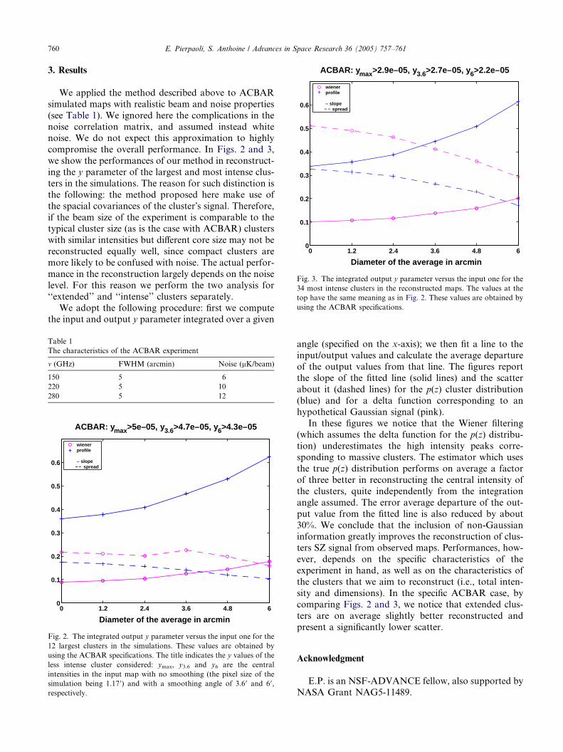
ACBAR: ymax>2.9e–05, y3.6>2.7e–05, y6>2.2e–05

wienerprofile

–– –

slope spread

Fig. 3. The integrated output y parameter versus the input one for the

34 most intense clusters in the reconstructed maps. The values at the

top have the same meaning as in Fig. 2. These values are obtained by

using the ACBAR specifications.

760 E. Pierpaoli, S. Anthoine / Advances in Space Research 36 (2005) 757–761

3. Results

We applied the method described above to ACBAR

simulated maps with realistic beam and noise properties

(see Table 1). We ignored here the complications in the

noise correlation matrix, and assumed instead whitenoise. We do not expect this approximation to highly

compromise the overall performance. In Figs. 2 and 3,

we show the performances of our method in reconstruct-

ing the y parameter of the largest and most intense clus-

ters in the simulations. The reason for such distinction is

the following: the method proposed here make use of

the spacial covariances of the cluster�s signal. Therefore,if the beam size of the experiment is comparable to thetypical cluster size (as is the case with ACBAR) clusters

with similar intensities but different core size may not be

reconstructed equally well, since compact clusters are

more likely to be confused with noise. The actual perfor-

mance in the reconstruction largely depends on the noise

level. For this reason we perform the two analysis for

‘‘extended’’ and ‘‘intense’’ clusters separately.

We adopt the following procedure: first we computethe input and output y parameter integrated over a given

Table 1

The characteristics of the ACBAR experiment

m (GHz) FWHM (arcmin) Noise (lK/beam)

150 5 6

220 5 10

280 5 12

0 1.2 2.4 3.6 4.8 60

0.1

0.2

0.3

0.4

0.5

0.6

Diameter of the average in arcmin

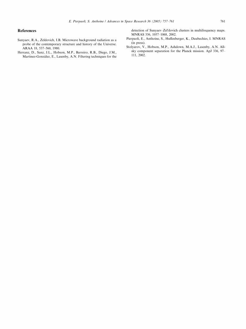
ACBAR: ymax>5e–05, y3.6>4.7e–05, y6>4.3e–05

wienerprofile

–– –

slope spread

Fig. 2. The integrated output y parameter versus the input one for the

12 largest clusters in the simulations. These values are obtained by

using the ACBAR specifications. The title indicates the y values of the

less intense cluster considered: ymax, y3.6 and y6 are the central

intensities in the input map with no smoothing (the pixel size of the

simulation being 1.17 0) and with a smoothing angle of 3.6 0 and 6 0,

respectively.

angle (specified on the x-axis); we then fit a line to the

input/output values and calculate the average departureof the output values from that line. The figures report

the slope of the fitted line (solid lines) and the scatter

about it (dashed lines) for the p(z) cluster distribution

(blue) and for a delta function corresponding to an

hypothetical Gaussian signal (pink).

In these figures we notice that the Wiener filtering

(which assumes the delta function for the p(z) distribu-

tion) underestimates the high intensity peaks corre-sponding to massive clusters. The estimator which uses

the true p(z) distribution performs on average a factor

of three better in reconstructing the central intensity of

the clusters, quite independently from the integration

angle assumed. The error average departure of the out-

put value from the fitted line is also reduced by about

30%. We conclude that the inclusion of non-Gaussian

information greatly improves the reconstruction of clus-ters SZ signal from observed maps. Performances, how-

ever, depends on the specific characteristics of the

experiment in hand, as well as on the characteristics of

the clusters that we aim to reconstruct (i.e., total inten-

sity and dimensions). In the specific ACBAR case, by

comparing Figs. 2 and 3, we notice that extended clus-

ters are on average slightly better reconstructed and

present a significantly lower scatter.

Acknowledgment

E.P. is an NSF-ADVANCE fellow, also supported by

NASA Grant NAG5-11489.

E. Pierpaoli, S. Anthoine / Advances in Space Research 36 (2005) 757–761 761

References

Sunyaev, R.A., Zeldovich, I.B. Microwave background radiation as a

probe of the contemporary structure and history of the Universe.

ARAA 18, 537–560, 1980.

Herranz, D., Sanz, J.L., Hobson, M.P., Barreiro, R.B., Diego, J.M.,

Martınez-Gonzalez, E., Lasenby, A.N. Filtering techniques for the

detection of Sunyaev–Zel�dovich clusters in multifrequency maps.

MNRAS 336, 1057–1068, 2002.

Pierpaoli, E., Anthoine, S., Huffenberger, K., Daubechies, I. MNRAS

(in press).

Stolyarov, V., Hobson, M.P., Ashdown, M.A.J., Lasenby, A.N. All-

sky component separation for the Planck mission. ApJ 336, 97–

111, 2002.