Finding the Equilibrium Real Interest Rate in a Fog of Policy Deviations

John B. Taylor and Volker Wieland

Economics Working Paper 16109

HOOVER INSTITUTION 434 GALVEZ MALL

STANFORD UNIVERSITY STANFORD, CA 94305-6010

April 2016

Recently there has been an explosion of research on whether the equilibrium real interest rate has declined, an issue with significant implications for monetary policy. A common finding is that the rate has declined. In this paper we provide evidence that contradicts this finding. We show that the perceived decline may well be due to shifts in regulatory policy and monetary policy that have been omitted from the research. In developing the monetary policy implications, it is promising that much of the research approaches the policy problem through the framework of monetary policy rules, as uncertainty in the equilibrium real rate is not a reason to abandon rules in favor of discretion. But the results are still inconclusive and too uncertain to incorporate into policy rules in the ways that have been suggested. The Hoover Institution Economics Working Paper Series allows authors to distribute research for discussion and comment among other researchers. Working papers reflect the views of the authors and not the views of the Hoover Institution.

1

Finding the Equilibrium Real Interest Rate in a Fog of Policy Deviations1

John B. Taylor and Volker Wieland

April 2016 A large number of economic research papers have recently been written endeavoring to

estimate the current level and trend in the equilibrium real interest rate. Examples include

Barsky, Justiniano and Melosi (2014), Curdia (2015), Curdia, Ferrero, Ng and Tambalotti

(2015), Justiniano and Primiceri (2012), Kiley (2015), Laubach and Williams (2015), and Lubik

and Matthes (2015). These studies are generally model-based: they either use semi-structural

time-series and filtering methods or formal structural dynamic stochastic general equilibrium

(DSGE) macroeconomic models to examine the relationship between the equilibrium real

interest rate and its possible determinants. A common finding in these studies is that the

equilibrium real interest rate has declined in recent years to a level not seen in decades.

The explosion of this research is not surprising. The results have important implications

for monetary policy as discussed in Carlstrom and Fuerst (2016), Dupor (2015), Hamilton,

Harris, Hatzius and West (2015), Summers (2014) and Yellen (2015). Indeed, several U.S.

policy making or policy advising organizations have reported estimates or ranges of estimates of

the equilibrium real interest rate based on such studies, including the Congressional Budget

Office, the Office of Management and Budget, the Federal Open Market Committee, as well as

professional forecasters and financial market participants, as Cieslak (2015) has documented.

1 This paper is based in part on results presented at the NABE Panel “The Equilibrium Real Interest Rate—Theory, Measurement, and Use in Monetary Policy” organized by George Kahn at the ASSA meeting in San Francisco on January 3, 2016

2

Many of the recommendations for monetary policy are in the form of how the central bank’s

monetary policy rule should be adapted, modified, or even thrown out in light of the findings.

Although much of the research is new, it can be traced to a 2003 paper by Laubach and

Williams (2003) on estimating the equilibrium interest rate. Until that time, as the authors then

noted, “the problem of real-time estimation of the natural rate of interest has received

surprisingly little attention” with one exception being Rudebusch’s (2001) analysis of the stance

of monetary policy. Prior to this period virtually all work on measurement uncertainty relating to

monetary policy rules was about estimates of potential GDP or measures of inflation, rather than

the equilibrium real interest rate.

In this paper we examine the underlying methodology used in these model-based

estimates. First, we show that the estimates are subject to omitted variable or even omitted

equation bias. What appear to be trends in the equilibrium interest rate may instead be trends in

other policy variables that affect the economy. While such problems have always made it

difficult to find and estimate concepts such as the equilibrium real interest rate, recent changes in

policy variables have deepened the fog. Second, we show that methods used to adjust monetary

policy rules to take account of shifts in the equilibrium interest rate alone are incomplete and

misleading because they do not incorporate other shifts—such as changes in potential GDP—that

are associated with the shifts. These shifts need to be accounted for when the results are applied

to monetary policy decisions or rules. Finally, we show that alternative simulation techniques

can radically alter the results. In sum we conclude that the estimates of time-varying real

equilibrium interest rates that have emerged from recent research are not yet useful for

application to current monetary policy.

3

A Simple Framework and Omitted Variables Problems

The real equilibrium interest rate is usually defined as the real interest rate consistent with

the economy reaching both potential output and price stability. In other words, it is the real

interest rate where real GDP equals potential GDP and the inflation rate equals the target

inflation rate.2 The semi-structural time-series and DSGE models used to find this equilibrium

real interest rate are complex and difficult to understand intuitively, but the logic—and thereby

the pitfalls—can be explained in simple terms if we focus on three relationships common to

macroeconomic models. The methodology described here is closest to that used by Laubach and

Williams (2015), but we think it also applies to the model-based studies such as Barsky,

Justiniano and Melosi (2014), Curdia et al (2015), or Justiniano and Primiceri (2012).3

The first relationship is the intertemporal substitution equation (aka Euler equation or IS

curve) between real GDP and the real interest rate. For simplicity we can write this as a linear

equation in terms of percentage deviations of real GDP from potential GDP and the deviations of

the real interest rate from the equilibrium real interest rate:

y - y* = - β(r-r*) (1)

where y is the log of real GDP, y* is the log of potential GDP, r is the real interest rate and r* is

the equilibrium real interest rate. Assume that we have time series observations on y and r, and

that the parameter β can be calibrated or estimated.

2 For example, this is the definition used in Yellen (2015). 3 Here we abstract from differences in timing of equilibrium and the definition of potential GDP. For example, some of the DSGE studies have focused on short-run equilibria that depend on economic shocks rather than the medium- or longer-run levels that are reached when the effects of shocks have been partly or fully resolved.

4

The second relationship is about price adjustment. Again for simplicity assume that it too

can be represented as a linear equation, this time between the rate of inflation and the gap

between real GDP and potential GDP

π = π(-1) + θ(y-y*) (2)

where π is the inflation rate. This equation could easily be generalized to incorporate staggered

wage setting, expectations, or indexing as in a typical new Keynesian model, but the logic of the

argument would not change. Note that having the gap on the right-hand side, implies that y

being equal to y* is consistent with price stability (steady inflation at a target, such as 2 percent).

We assume that we have observations on π and that the parameter θ can also be calibrated or

estimated.

Model-based studies focus on these two relationships and the task is to use them to find

the equilibrium real rate of interest r*. If one knew potential GDP (y*), then a seemingly

reasonable method for finding r* would be to see if equation (1) generates an output gap (y-y*)

that is different from what is predicted, P(y-y*), based on information on the right hand side. If

there is a difference, then one must adjust (the estimate of) r* up or down until it gives the

correct prediction. For example, if (y-y*) < P(y-y*), then r* is too high and it must be lowered.

Of course, y* is also unknown, but equation (2) can be used to help find it following the

same logic used to find r*: If π is not equal to the prediction, Pπ, from equation (2), then adjust

y*. For example, if π > Pπ, then lower (the estimate of) y*.

Now consider the omitted variable problem. Suppose that another variable, or several

variables, can shift the intertemporal relationship in equation (1) around. For example, costly

5

regulations might lower the level of investment demand associated with a given real interest rate.

This would mean that rather than equation (1) we would have equation (1’)

y - y* = - β(r-r*) - αx* (1’)

where the variable x* could represent a variety of influences on real GDP from regulations that

negatively affect investment to tax policy that negatively affects consumption. With equation

(1’), if one finds that y-y* is lower than the prediction P(y-y*), then the implication is not

necessarily that the estimate of r* is too high and must be lowered. Now there is the possibility

that x* is too low and must be raised. In other words, the possibility of an omitted variable that

is not in the macro model makes it more difficult to find the equilibrium real interest rate.

There is also another important problem of omission which makes it even more difficult

to find r*. According to most macroeconomic models, there is also a financial sector and a

central bank reaction function which create another relationship. To capture this relationship

suppose we add a monetary policy rule to the model which makes the nominal interest rate and

thus the real interest rate endogenous:

i= π + .5(π-2) + .5(y-y*) + r* + d* (3)

where i is the nominal interest rate set by the central bank and d* is a possible deviation from the

policy implied by the rule. As with equations (1) and (2), if i is not equal to the prediction Pi,

then one can adjust r*, but one can also adjust d*. For example, if i < Pi then one might

conclude that it reflects a lower r*, but an alternative interpretation is a decline in d*. In fact,

6

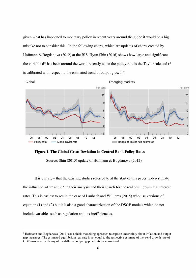
given what has happened to monetary policy in recent years around the globe it would be a big

mistake not to consider this. In the following charts, which are updates of charts created by

Hofmann & Bogdanova (2012) at the BIS, Hyun Shin (2016) shows how large and significant

the variable d* has been around the world recently when the policy rule is the Taylor rule and r*

is calibrated with respect to the estimated trend of output growth.4

Figure 1. The Global Great Deviation in Central Bank Policy Rates

Source: Shin (2015) update of Hofmann & Bogdanova (2012)

It is our view that the existing studies referred to at the start of this paper underestimate

the influence of x* and d* in their analysis and their search for the real equilibrium real interest

rates. This is easiest to see in the case of Laubach and Williams (2015) who use versions of

equation (1) and (2) but it is also a good characterization of the DSGE models which do not

include variables such as regulation and tax inefficiencies.

4 Hofmann and Bogdanova (2012) use a thick-modelling approach to capture uncertainty about inflation and output gap measures. The estimated equilibrium real rate is set equal to the respective estimate of the trend growth rate of GDP associated with any of the different output gap definitions considered.

7

Implication for the Pre-Crisis and Post-Crisis Equilibrium Real Interest Rate

Let us now consider in more detail the implications of the omitted variables during the

past 15 years, the period over which much of the research on the equilibrium real interest rate has

been conducted. The story is different for the pre-crisis period, especially from 2003 to 2005,

compared to post-crisis period, so we consider each separately.

Pre-Crisis Period

During the period around 2003-2005, the U.S. economy was generally booming. The

unemployment rate got as low as 4.4% well below the natural rate, a clear indication that y was

greater than y*. There were extraordinary upward pressures in the housing market as demand for

homes skyrocketed and home price inflation took off. And overall inflation was rising. The

inflation rate measured by the GDP price index doubled from 1.7% to 3.4% per year. In sum,

there were clear signs of overheating with y greater than y* and π rising.

During this period the Fed held its policy interest rate (the federal funds rate) very low at

1 percent for a “prolonged period” and then increased it very slowly at a “measured pace.” It

thus appeared that r<r* and, as predicted by equations (1) and (2), this created upward pressures

on y and π. In other words, the model was generally predicting well and there is no reason to

think that r* should have been lower than 2 percent during that period. Since y was above y*,

there is no reason to adjust y* on that account either.

These interest rate settings were below the policy rule in equation (3) for a r* =2 and d* =

0. According to equation (3), this implies either that r* should be adjusted down, say from 2

percent to 0 percent, or that d* should be adjusted down, say from 0 percent to -2 percent. With

8

no reason to lower the equilibrium rate based on equation (1) and (2), however, the explanation

must be that policy rate deviated from the policy rule. In fact, there is corroborating evidence for

this, including Shin’s (2016) graph in Figure 1. In other words, the evidence points to a policy

deviation d* which shifted the Fed’s policy rate down, rather than a decline in r*.

In contrast, note that Summers (2014) argues that r* had fallen in the years before the

crisis, when, as he put it, “arguably inappropriate monetary policies and surely inappropriate

regulatory policies,” should have caused the economy to overheat. Since Summers also argues

that “there is almost no case to be made that the real US economy overheated prior to the crisis”

he concludes that r* should be lower. But in fact, as shown in the previous paragraph, the

economy did overheat in that period—whether one looks at labor market pressures, rising

inflation, or boom-like housing conditions. By bringing in the third equation and the missing

variable d* one has the alternative explanation given here.

Post-Crisis Period

Now consider the years after the crisis. During these years, the economic recovery has

been very weak as many authors have concluded. The gap between real GDP and potential

GDP—at least as measured before the crisis—has not closed by much. Many, including

economists at the Federal Reserve Board, predicted that the recovery would be stronger. It is

clear that y-y* was lower than forecast with the very low interest rate set by the Federal Reserve.

Most of the studies referred to at the start of this paper argue that the forecast error is due

to an r* that is lower than we thought, and this gives rise to the idea of a currently low r*. If r* is

down, then r-r* is not as low as you think. But according to equation (1’), it could either be a

lower r* or a higher x* that is dragging the economy down at a given real interest rate r. Thus an

9

an alternative explanation is x* has been the problem. And there is corroborating evidence of

this. Most of the contributors to the book by Ohanian, Taylor and Wright (2012) argue that the

problem is economic policy.

But if you want to point to x* rather than r* as the culprit then how do you explain the

very low interest rates set by the Federal Reserve and other central banks. Here is where equation

(3) and the other omitted variable come in. A decline in r* is not the only reason why the interest

rate is low. It could just as well be due to a policy deviation d*. And here there is corroborating

evidence. Figure 1 shows that the decline may well be due to a large deviation d*—what

Hofmann and Bogdanova (2012) call a Global Great Deviation—rather than r* being the culprit.

In sum there is a perfectly reasonable alternative explanation of the facts if one expands

the model as suggested here. Rather than conclude that the real equilibrium interest rate r* has

declined, there is the alternative that economic policy has deviated shifted, whether in the form

of regulatory and tax policy (x*) or in the form if monetary policy (d*). And there is empirical

evidence in favor of this explanation.

Implications for Monetary Policy

Many have explored the policy implications of the research on the real equilibrium

interest rate, and this usually is in the context of how to adjust the central bank’s monetary policy

rules. In an important recent speech, Yellen (2015), for example, showed the effects of allowing

a change in the equilibrium real interest rate in the Taylor rule, arguing as follows5

“Taylor’s rule now calls for the federal funds rate to be well above zero if… the

“normal” level of the real federal funds rate is currently close to its historical average.

5 Yellen (2015) uses slightly different notation, such as RR* rather than r*

10

But the prescription offered by the Taylor rule changes significantly if one instead

assumes, as I do, that the economy’s equilibrium real federal funds rate–that is, the real

rate consistent with the economy achieving maximum employment and price stability

over the medium term–is currently quite low by historical standards. Under assumptions

that I consider more realistic under present circumstances, the same rules call for the

federal funds rate to be close to zero…

“For example, the Taylor rule is Rt = RR* + πt + 0.5(πt -2) + 0.5Yt, where R

denotes the federal funds rate, RR* is the estimated value of the equilibrium real rate, π

is the current inflation rate (usually measured using a core consumer price index), and Y

is the output gap. The latter can be approximated using Okun's law, Yt = -2 (Ut - U*),

where U is the unemployment rate and U* is the natural rate of unemployment. If RR*

is assumed to equal 2 percent (roughly the average historical value of the real federal

funds rate) and U* is assumed to equal 5-1/2 percent, then the Taylor rule would call for

the nominal funds rate to be set a bit below 3 percent currently, given that core PCE

inflation is now running close to 1-1/4 percent and the unemployment rate is 5.5

percent. But if RR* is instead assumed to equal 0 percent currently (as some statistical

models suggest) and U* is assumed to equal 5 percent (an estimate in line with many

FOMC participants' SEP projections), then the rule's current prescription is less than 1/2

percent.”

Thus if one simply replaces the equilibrium federal funds rate of 2% in the Taylor rule

with 0%, then the recommended setting for the funds rate declines by two percentage points.

11

However, there is a lot of disagreement and uncertainty regarding this rate, and in our view, there

are good reasons to think that it has not changed that much.

In any case this is a controversial and debatable issue, deserving a lot of research. If one

can adjust the intercept term (that is, RR*) in a policy rule in a purely discretionary way, then it

is not a rule at all any more. It’s purely discretion. Sharp changes in the equilibrium interest rate

need to be treated very carefully.6

Moreover, calculations such as in Yellen (2015) are incomplete and misleading because

they do not incorporate other shifts—such as changes in potential GDP—that are associated with

the shifts in r* according to Laubach-Williams (2015) and others. As she describes in her paper,

Yellen (2015) shows that if you insert estimates of the equilibrium interest rate computed by

Laubach and Williams (2015) into a Taylor rule, you get a lower policy interest rate in the

United States than if you assume a 2 percent real rate as in the original version of the rule.

However, as the Report of the German Council of Economic Experts (2015)7 shows, that’s not

true if you also insert, along with the estimated real equilibrium interest rate, the associated real

output gap estimated with the Laubach-Williams methodology as logic and consistency would

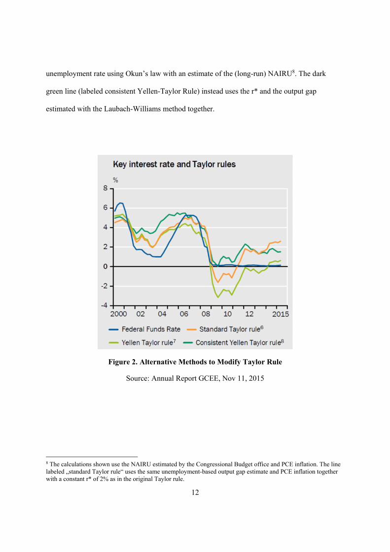
suggest. Figure 2 below, drawn from the GCEE Report shows that the effect is very large—more

than 2 percentage points. It thus completely reverses the impact of the lower r*. The light-green

line (labeled Yellen-Taylor rule) shows the Yellen (2015) version of the Taylor rule that uses the

estimate of r* from the Laubach-Williams method together with an output gap derived from the

6 Another important rules versus discretion issue illustrated by Yellen’s (2015) paper is that she does not make the argument here that the coefficient on the output gap in the Taylor rule should be 1.0 rather than 0.5 as she has in previous speeches advocating a lower interest rate. The argument is different here, and no reason for dropping the old argument is given. Perhaps the reason is that the gap is small now, so the coefficient on the gap does not make much difference. Nevertheless, this gives the impression that one is changing the rule to get a desired result. 7 One of the authors of this paper, Volker Wieland, is a member of the Council and co-author of the Annual Report.

12

unemployment rate using Okun’s law with an estimate of the (long-run) NAIRU8. The dark

green line (labeled consistent Yellen-Taylor Rule) instead uses the r* and the output gap

estimated with the Laubach-Williams method together.

Figure 2. Alternative Methods to Modify Taylor Rule

Source: Annual Report GCEE, Nov 11, 2015

8 The calculations shown use the NAIRU estimated by the Congressional Budget office and PCE inflation. The line labeled „standard Taylor rule“ uses the same unemployment-based output gap estimate and PCE inflation together with a constant r* of 2% as in the original Taylor rule.

13

There are several other suggestions for how to adjust monetary rules in light of new

estimates of r*. Laubach and Williams (2015) and Hamilton, Harris, Hatzius and West (2015)

argue that uncertainty about r* means that policy makers should use inertial Taylor rules, with a

lagged interest rate on the right hand side along with other variables. There are other reasons for

doing this in the literature and it is not a very radical idea.

Other suggestions are more radical. Curdia, Ferrero, Ng, and Tambalotti (2015) suggest

replacing the output gap in the Taylor rule with r*, arguing that economic performance would

improve. Barsky, Justiniano, Melosi (2014) suggest doing away with the Taylor rule altogether

and just setting the policy interest rate to r* as it is estimated to move around over time. In our

view the estimates of r* are still way too uncertain, and more evidence about robustness is

needed before following these suggestions.

Alternative Simulation Techniques

Studies that use New Keynesian DSGE models to estimate time-varying equilibrium real

interest rates such as, for example, Barsky et al (2014) and Curdia et al (2015), have focused on

simulating the path of a short-run equilibrium rate. It is the real interest rate that coincides with

the level of output that would result under a fully flexible price level, that is, absent the price

level rigidity characteristic of New Keynesian models. This short-run equilibrium rate depends

on economic shocks and consequently varies a lot over time. It could even exhibit greater

variation than the actual real interest rate.

Of course, DSGE models also contain a long-run equilibrium real interest rate. It is

reached in steady-state when the effects of economic shocks have worked themselves out. This is

the rate that has typically been used as r* in model-based evaluations of policy rules of the form

14

of equation (3), including, for example, the comparative studies in Taylor (1999), Levin,

Wieland and Williams (2003) and Taylor and Wieland (2012). One of the models considered in

the latter comparison is the well-known empirical New Keynesian DSGE model of the United

States economy estimated by Smets and Wouters (2007). They report an estimate of the steady-

state real interest rate of 3 percent based on quarterly data of 2005 vintage covering the period of

1996:Q1 to 2004:Q4.

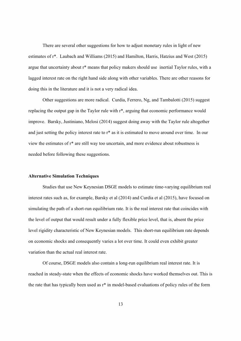
Figure 3 below, also drawn from the GCEE Report (2015), shows that estimates of the

long-run equilibrium real rate have not changed that much. These estimates are based on rolling

20-year windows of real time data. Thus, each quarter the model is fit to the data vintage

available at that period in time using the same Bayesian estimation method as Smets and

Wouters (2007). The resulting equilibrium rate is about 3 percent in 1994. Afterwards, estimates

rises slowly to values closer 4 percent. From 2002 onwards they decline again slowly towards

about 3 percent in 2007. In recent years, the long-run equilibrium is estimated a bit above 2

percent.9 Thus, estimates of the long-run r* based on a very standard DSGE model vary little and

remain well above zero.

9 Estimates of the long-run real rate within such a DSGE model using Bayesian methods depend on empirical averages as well as the model structure including the priors set by the modeler concerning certain structural parameters. The above estimation uses the same priors as Smets and Wouters. There is no prior set on the equilibrium interest rate. It is likely to be influenced by the priors for equilibrium inflation, equilibrium GDP growth, the discount rate and the intertemporal elasticity of substitution. Estimates of the equilibrium interest rate vary less than the 20-year sample averages of the real interest rate.

15

Figure 3: Estimates of long-run r* with the Smets-Wouters model

Source: Annual Economic Report German Council of Economic Experts 2015

Figure 3 also includes estimates of equilibrium inflation, which remain very stable, and

the equilibrium nominal interest rate, which mirror the moderate changes in the real rate. The

use of rolling 20-year windows implies giving a lot of weight to recent data in estimating the

equilibrium rate. If one simply extends the original data range to include the more recent

observations, the estimate of the equilibrium rate will decline even less.

Conclusion

There has been much interesting model-based research recently on the question of

whether the equilibrium real interest rate r* has declined or not. However, we do not think this

research is yet useful for policy because it omits important variables relating to structural policy

and monetary policy. In developing the monetary policy implications, the research is promising

in that it approaches the policy problem through the framework of monetary policy rules, as

16

uncertainty in the equilibrium real rate is not a reason to abandon rules in favor of discretion.

Nevertheless, the results are still inconclusive and too uncertain to incorporate into policy rules

in the ways that have been suggested.

Furthermore, there is evidence that contradicts the hypothesis that there has been a

significant decline in the equilibrium real interest rate. Instead, the perceived decline found in

recent studies may well be due to shifts in regulatory policy and monetary policy that have been

omitted from the research.

17

References

Barsky, Robert, Alejandro Justiniano, and Leonardo Melosi (2014), The Natural Rate of Interest and Its Usefulness for Monetary Policy,” American Economic Review: Papers & Proceedings, 104(5): 37–43.

Carlstrom and Charles T. and Timothy S. Fuerst (2016), “The Natural Rate of Interest in Taylor Rules,” Economic Commentary, No. 2016-01, Federal Reserve Bank of Cleveland.

Cieslak, Anna (2015) “Discussion of ‘The Equilibrium Real Funds Rate: Past, Present and Future,’” by James D. Hamilton, Ethan S. Harris, Jan Hatzius, Kenneth D. West (2015), slides from Brookings Conference, http://www.brookings.edu/~/media/Events/2015/10/interest-rates/Disc_HHHW_02.pdf?la=en.

Curdia, Vasco (2015), “Why So Slow? A Gradual Return for Interest Rates,” FRBSF Economic Letter, October 12.

Curdia, Vasco, Andrea Ferrero, Ging Cee Ng, Andrea Tambalotti (2015), “Has U.S. Monetary Policy Tracked the Efficient Interest Rate?” Journal of Monetary Economics, Vol. 70(C), 72-83.

Dupor, William (2015) “Liftoff and the Natural Rate of Interest”, Economic Synopsis, No. 12 Federal Reserve Bank of St. Louis.

German Council of Economic Experts (2015) Focus on Future Viability Annual Economic Report, November 11.

Hamilton, James D., Ethan S. Harris, Jan Hatzius, Kenneth D. West (2015), “The Equilibrium Real Funds Rate: Past, Present and Future,” paper for the U.S. Monetary Policy Forum, New York City, February 27.

Hofmann, Boris and Bilyana Bogdanova, 2012, Taylor Rules and Monetary Policy: A Global Great Deviation? BIS Quarterly Review, September.

Justiniano, Alejandro and Giorgio E. Primiceri (2010) “Measuring the equilibrium real interest rate,” Economic Perspectives, Federal Reserve Bank of Chicago.

Kiley, Michael T. (2015), “What Can the Data Tell Us About the Equilibrium Real Interest Rate?” Board of Governors of the Federal Reserve, FEDS Working Paper No. 2015-077.

Laubach, Thomas and John C. Williams, 2003, “Measuring the Natural Rate of Interest,” The Review of Economics and Statistics 85(4): 1063-1070.

Laubach, Thomas and John C. Williams, 2015, “Measuring the Natural Rate of Interest Redux,” Federal Reserve Bank of San Francisco.

18

Levin, Andrew, John C. Williams and Volker Wieland (2003), The Performance of Forecast-Based Monetary Policy Rules under Model Uncertainty, American Economic Review, 93 (3), June.

Lubik, Thomas A. and Christian Matthes (2015), “Calculating the Natural Rate of Interest: A Comparison of Two Alternative Approaches,” Economic Brief, Federal Reserve Bank of Richmond, October.

Orphanides, Athanasios, and John C. Williams, (2002), “Robust Monetary Policy Rules with Unknown Natural Rates,” Brookings Papers on Economic Activity, 2, 63–145.

Rudebusch, Glenn D. (2001), “Is the Fed Too Timid? Monetary Policy in an Uncertain World,” (2001) Review of Economics and Statistics 83:2 203–217.

Shin, Hyun (2016) “Macroprudential Tools, Their Limits, and Their Connection with Monetary Policy” in Olivier Blanchard, Raghuram Rajan, Kenneth Rogoff, and Lawrence H. Summers (Eds.), Progress and Confusion: The State of Macroeconomic Policy, MIT Press.

Smets, Frank and Raf Wouters (2007), Shocks and Frictions in US Business Cycles: A Bayesian DSGE Approach, American Economic Review, 97:3, 586-606, June.

Summers, Lawrence H. (2014), “Low Equilibrium Real Rates, Financial Crisis, and Secular Stagnation,” in Martin Neil Baily, John B. Taylor (Eds.) Across the Great Divide: New Perspectives on the Financial Crisis. Hoover Press, Stanford, pp. 37-50 http://www.hoover.org/sites/default/files/across-the-great-divide-ch2.pdf.

Taylor, John B.(1999) (ed.), Monetary Policy Rules, University of Chicago Press.

Taylor, John B. and Volker Wieland (2012), Surprising Comparative Properties of Monetary Models: Results from a New Model Data Base, Review of Economics and Statistics,94 (3), August 2012, pp. 800-816.

Yellen, Janet (2015), “Normalizing Monetary Policy: Prospects and Perspectives,” Remarks at the conference on New Normal Monetary Policy, Federal Reserve Bank of San Francisco.