Fine-grained Categorization and Dataset Bootstrapping using Deep Metric

Learning with Humans in the Loop

Yin Cui1,2 Feng Zhou3 Yuanqing Lin3 Serge Belongie1,2

1Department of Computer Science, Cornell University 2Cornell Tech 3NEC Labs America1,2{ycui, sjb}@cs.cornell.edu 3{feng, ylin}@nec-labs.com

Abstract

Existing fine-grained visual categorization methods of-

ten suffer from three challenges: lack of training data,

large number of fine-grained categories, and high intra-

class vs. low inter-class variance. In this work we pro-

pose a generic iterative framework for fine-grained catego-

rization and dataset bootstrapping that handles these three

challenges. Using deep metric learning with humans in the

loop, we learn a low dimensional feature embedding with

anchor points on manifolds for each category. These an-

chor points capture intra-class variances and remain dis-

criminative between classes. In each round, images with

high confidence scores from our model are sent to humans

for labeling. By comparing with exemplar images, labelers

mark each candidate image as either a “true positive” or

a “false positive.” True positives are added into our cur-

rent dataset and false positives are regarded as “hard nega-

tives” for our metric learning model. Then the model is re-

trained with an expanded dataset and hard negatives for the

next round. To demonstrate the effectiveness of the proposed

framework, we bootstrap a fine-grained flower dataset with

620 categories from Instagram images. The proposed deep

metric learning scheme is evaluated on both our dataset and

the CUB-200-2001 Birds dataset. Experimental evaluations

show significant performance gain using dataset bootstrap-

ping and demonstrate state-of-the-art results achieved by

the proposed deep metric learning methods.

1. Introduction

Fine-grained visual categorization (FGVC) has received

increased interest from the computer vision community in

recent years. By definition, FGVC, as a sub-field of ob-

ject recognition, aims to distinguish subordinate categories

within an entry-level category. For example, in fine-grained

flower categorization [33, 34, 3], we want to identify the

species of a flower in an image, such as “nelumbo nucifera

Fine-grained flower classifier

trained with deep metric learning

Confidence > 50%

u11 u12

u13

u21

u22

u23

input

“lotus flower” manifold

“tulip” manifold

…

…

Candidate flower images

“lotus flower” candidates

“tulip” candidates

…

…

lotus flower?

yes!

exemplar lotus flowers

and description

Human labeling

True positives False positives

Dataset Expansion

lotus flower“hard negatives” for lotus flower

tulip…

“hard negatives” for tulip

…

lotus flower

tulip

…

Figure 1. Overview of the proposed framework. Using deep metric

learning with humans in the loop, we learn a low dimensional fea-

ture embedding for each category that can be used for fine-grained

visual categorization and iterative dataset bootstrapping.

(lotus flower),” “tulip” or “cherry blossom.” Other exam-

ples include classifying different types of plants [28], birds

[7, 6], dogs [24], insects [30], galaxies [13, 11]; recogniz-

ing brand, model and year of cars [26, 46, 48]; and face

identification [39, 36].

Most existing FGVC methods fall into a classical two-

step scheme: feature extraction followed by classification

[1, 5, 8, 35]. Since these two steps are independent, the

performance of the whole system is often suboptimal com-

pared with an end-to-end system using Convolutional Neu-

ral Networks (CNN) that can be globally optimized via

back-propagation [6, 50, 25, 32]. Therefore, in this work,

we focus on developing an end-to-end CNN-based method

for FGVC. However, compared with general purpose visual

categorization, there are three main challenges arising when

11153

Lotus

flower

Nymphaea

FGVC

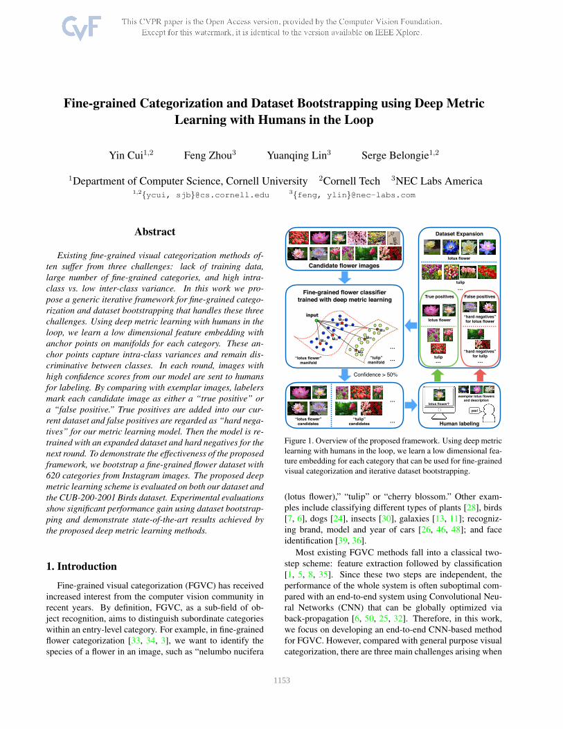
Figure 2. Simple appearance based methods will likely find in-

correct groups for two visually similar categories. A successful

FGVC approach should be able to deal with the challenge of high

intra-class vs. low inter-class variance.

using such end-to-end CNN-based systems for FGVC.

Firstly, lack of training data. Current commonly used

CNN architectures such as AlexNet [27], VGGNet [37],

GoogLeNet-Inception [38] and ResNet [19] have large

numbers of parameters that require vast amounts of training

data to achieve reasonably good performance. Commonly

used FGVC databases [34, 7, 24, 26], however, are rela-

tively small, typically with less than a few tens of thousands

of training images.

Secondly, compounding the above problem, FGVC can

involve large numbers of categories. For example, ar-

guably, it is believed that there are more than 400, 000species of flowers in the world [23]. As a point of refer-

ence, modern face identification systems need to be trained

on face images coming from millions of different identities

(categories). In such scenarios, the final fully connected

layer of a CNN before the softmax layer would contain too

many nodes, thereby making the training infeasible.

Lastly, high intra-class vs. low inter-class variance.

In FGVC, we confront two somewhat conflicting require-

ments: distinguishing visually similar images from differ-

ent categories while allowing reasonably large variability

(pose, color, lighting conditions, etc.) within a category. As

an example illustrated in Fig. 2, images from different cat-

egories could have similar shape and color. On the other

hand, sometimes images within same category can be very

dissimilar due to nuisance variables. In such a scenario,

since approaches that work well on generic image classi-

fication often focus on inter-class differences rather than

intra-class variance, directly applying them to FGVC could

make visually similar categories hard to be distinguished.

In this paper, we propose a framework that aims to ad-

dress all three challenges. We are interested in the follow-

ing question: given an FGVC task with its associated train-

ing and test set, are we able to improve the performance

by bootstrapping more training data from the web? In light

of this, we propose a unified framework using deep metric

learning with humans in the loop, illustrated in Fig. 1.

We use an iterative approach for dataset bootstrapping

and model training. In each round, the model trained from

last round is used to generate fine-grained confidence scores

(probability distribution) for all the candidate images on

categories. Only images with highest confidence score

larger than a threshold are kept and put into the correspond-

ing category. Then, for each category, by comparing with

exemplar images and category definitions, human labelers

remove false positives (hard negatives). Images that pass

the human filtering will be included into the dataset as new

(vetted) data. Finally, we re-train our classification model

by incorporating newly added data and also leveraging the

hard negatives marked by human labelers. The updated

model will be used for the next round of dataset bootstrap-

ping. Although we focus on flower categorization in this

work, the proposed framework is applicable to other FGVC

tasks.

In order to capture within-class variance and utilize hard

negatives as well, we propose a triplet-based deep metric

learning approach for model training. A novel metric learn-

ing approach enables us to learn low-dimensional manifolds

with multiple anchor points for each fine-grained category.

These manifolds capture within-category variances and re-

main discriminative to other categories. The data can be

embedded into a feature space with dimension much lower

than the number of categories. During the classification, we

generate the categorical confidence score by using multiple

anchor points located on the manifolds.

In summary, the proposed framework handles all three

challenges in FGVC mentioned above. Using the proposed

framework, we are able to grow our training set and get a

better fine-grained classifier as well.

2. Related Work

Fine-Grained Visual Categorization (FGVC). Many

approaches have been proposed recently for distinguishing

between fine-grained categories. Most of them [1, 5, 8, 35]

use two independent steps: feature extraction and classi-

fication. Fueled by the recent advances in Convolutional

Neural Networks (CNN) [27, 16], researchers have gravi-

tated to CNN features [6, 50, 25, 35, 32] rather than tra-

ditional hand-crafted features such as LLC [2] or Fisher

Vectors [14]. Sometimes, the information from segmen-

tation [25], part annotations [6], or both [8] is also used

during the feature extraction. Current state-of-the-art meth-

ods [6, 50, 25, 32] all adopt CNN-based end-to-end schemes

that learn feature representations from data directly for clas-

sification. Although our method also draws upon a CNN-

based scheme, there are two major differences. 1) Rather

than using softmax loss, we aim to find a low-dimensional

feature embedding for classification. 2) We incorporate hu-

mans into the training loop, with the human-provided input

contributing to the training of our model.

Fine-Grained Visual Datasets. Popular fine-grained vi-

sual datasets [34, 43, 24, 26] are relatively small scale, typ-

ically consisting of around 10 thousand training images or

less. There are some efforts recently in building large-scale

1154

fine-grained datasets [40, 48]. We differ from these efforts

both in terms of our goal and our approach. Instead of

building a dataset from scratch, we aim to bootstrap more

training data to enlarge the existing dataset we have. In ad-

dition, instead of human labeling, we also use a classifier

to help during the dataset bootstrapping. The most similar

work in terms of dataset bootstrapping comes from Yu et

al. [49], which builds a large-scale scene dataset with 10common categories using deep learning with humans in the

loop. However, we are bootstrapping a fine-grained dataset

with much more categories (620). Moreover, instead of a

dataset, we can also get a model trained with combined

human-machine efforts.

Deep Metric Learning. Another line of related work is

metric learning with CNNs using pairwise [10, 18] or triplet

constraints [44, 36, 21]. The goal is to use a CNN with

either pairwise (contrastive) or triplet loss to learn a fea-

ture embedding that captures the semantic similarity among

images. Compared with traditional metric learning meth-

ods that rely on hand-crafted features [47, 17, 45, 9], deep

metric learning directly learns from data and achieves much

better performance. Recently, it has been successfully ap-

plied to variety of problems including face recognition and

verification [39, 36], image retrieval [44], semantic hash-

ing [29], product design [4], geo-localization [31] and style

matching [41]. In contrast with previous methods, we pro-

pose a novel strategy that enables the learning of continuous

manifolds. In addition, we also bring humans in the loop

and leverage their inputs during metric learning.

3. Dataset Bootstrapping

One of the main challenges in fine-grained visual recog-

nition is the scarcity of training data. Labeling of fine-

grained categories is tedious because it calls for experts

with specialized domain knowledge. This section presents

a bootstrapping framework on how to grow a small scale,

fine-grained dataset in an efficient manner.

3.1. Discovering Candidate Images

In this first step, we wish to collect a large pool of can-

didate images for fine-grained subcategories under a coarse

category, e.g., flowers. The most intuitive way to crawl im-

ages could resort to image search engines like Google or

Bing. However, those returned images are often iconic, pre-

senting a single, centered object with a simple background,

which is not representative of natural conditions.

On the other hand, with the prevalence of powerful per-

sonal cameras and social networks, people capture their

day-to-day photos and share them via platforms like In-

stagram or Flickr. Those natural images uploaded by web

users offer us a rich source of candidate images, often with

tags that hint at the semantic content. So if we search

“flower” on Instagram, a reasonable portion of returned im-

ages should be flower images. Naturally, we will need a

filtering process to exclude the non-flower images.

We first downloaded two million images tagged with

“flower” via the Instagram API. To remove the images that

clearly contain no flowers, we pre-trained a flower classifier

based on GoogLeNet-Inception [38] with 70k images. By

feeding all the downloaded images to this classifier, we re-

tained a set of nearly one million images, denoted as C, with

confidence score larger than 0.5.

3.2. Dataset Bootstrapping with Combined Human­Machine Efforts

Given an initial fine-grained dataset S0 of N categories

and a candidate set C, the goal of dataset bootstrapping is to

select a subset S of the images from C that match with the

original N categories. We divided the candidate set into a

list of k subsets: C = C1∪C2∪· · ·∪Ck and used an iterative

approach for dataset bootstrapping with k iterations in total.

Each iteration consists of three steps. Consider the i-th

iteration. First, we trained a CNN-based classifier (see Sec.

4) using the seed dataset Si−1∪Hi−1, whereHi−1 contains

the hard negatives from the previous step. Second, using

this classifier, we assigned each candidate image x ∈ Cito one of the N categories. Images with confidence score

larger than 0.5 form a high quality candidate setDi ⊂ Ci for

the original N categories. Third, we asked human labelers

with domain expertise to identify true positives Ti and false

positives Fi, where Ti ∪ Fi = Di. Exemplar images and

category definitions were shown to the labelers.

Compared to the traditional process requiring the labeler

to select one of N categories per image, we asked labelers

to focus on a binary decision task which entails significantly

less cognitive load. Noting that these false positives Fi are

very similar to ground-truths, we regard them as hard nega-

tivesHi ← Hi−1∪Fi. True positives were also included to

expand our dataset: Si ← Si−1 ∪ Ti for the next iteration.

It is worth mentioning this bootstrapping framework is

similar in spirit to the recent work [42, 20] that used semi-

automatic crowdsourcing strategy to collect and annotate

videos. However, the key difference is we design a deep

metric learning method (see Sec. 4) that specifically makes

the use of the large number of hard negatives Hi in each

iteration.

4. Deep Metric Learning for FGVC

We frame our problem as a deep metric learning task.

We choose metric learning for mainly two reasons. First,

compared with classic deep networks that use softmax

loss in training, metric learning enables us to find a low-

dimensional embedding that can well capture high intra-

class variance. Second, metric learning is a good way

to leverage human-labeled hard negatives. It is often dif-

ficult to get categorical labels for these hard negatives.

1155

c2

c1

c3

c2

c1

c3

c4

c5

CNN with softmax loss CNN for metric learning

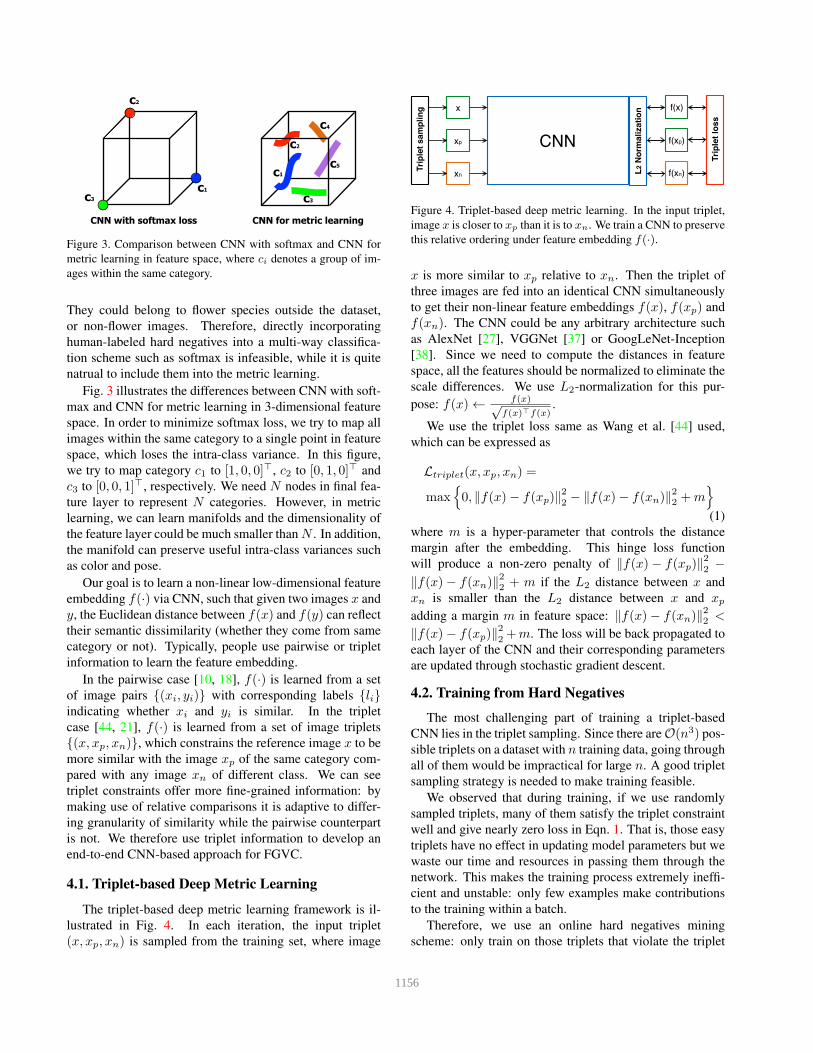
Figure 3. Comparison between CNN with softmax and CNN for

metric learning in feature space, where ci denotes a group of im-

ages within the same category.

They could belong to flower species outside the dataset,

or non-flower images. Therefore, directly incorporating

human-labeled hard negatives into a multi-way classifica-

tion scheme such as softmax is infeasible, while it is quite

natrual to include them into the metric learning.

Fig. 3 illustrates the differences between CNN with soft-

max and CNN for metric learning in 3-dimensional feature

space. In order to minimize softmax loss, we try to map all

images within the same category to a single point in feature

space, which loses the intra-class variance. In this figure,

we try to map category c1 to [1, 0, 0]⊤, c2 to [0, 1, 0]⊤ and

c3 to [0, 0, 1]⊤, respectively. We need N nodes in final fea-

ture layer to represent N categories. However, in metric

learning, we can learn manifolds and the dimensionality of

the feature layer could be much smaller than N . In addition,

the manifold can preserve useful intra-class variances such

as color and pose.

Our goal is to learn a non-linear low-dimensional feature

embedding f(·) via CNN, such that given two images x and

y, the Euclidean distance between f(x) and f(y) can reflect

their semantic dissimilarity (whether they come from same

category or not). Typically, people use pairwise or triplet

information to learn the feature embedding.

In the pairwise case [10, 18], f(·) is learned from a set

of image pairs {(xi, yi)} with corresponding labels {li}indicating whether xi and yi is similar. In the triplet

case [44, 21], f(·) is learned from a set of image triplets

{(x, xp, xn)}, which constrains the reference image x to be

more similar with the image xp of the same category com-

pared with any image xn of different class. We can see

triplet constraints offer more fine-grained information: by

making use of relative comparisons it is adaptive to differ-

ing granularity of similarity while the pairwise counterpart

is not. We therefore use triplet information to develop an

end-to-end CNN-based approach for FGVC.

4.1. Triplet­based Deep Metric Learning

The triplet-based deep metric learning framework is il-

lustrated in Fig. 4. In each iteration, the input triplet

(x, xp, xn) is sampled from the training set, where image

CNN

x

xp

xn

f(x)

f(xp)

f(xn) Tri

ple

t s

am

plin

g

L2 N

orm

aliza

tio

n

Tri

ple

t lo

ss

Figure 4. Triplet-based deep metric learning. In the input triplet,

image x is closer to xp than it is to xn. We train a CNN to preserve

this relative ordering under feature embedding f(·).

x is more similar to xp relative to xn. Then the triplet of

three images are fed into an identical CNN simultaneously

to get their non-linear feature embeddings f(x), f(xp) and

f(xn). The CNN could be any arbitrary architecture such

as AlexNet [27], VGGNet [37] or GoogLeNet-Inception

[38]. Since we need to compute the distances in feature

space, all the features should be normalized to eliminate the

scale differences. We use L2-normalization for this pur-

pose: f(x)← f(x)√f(x)⊤f(x)

.

We use the triplet loss same as Wang et al. [44] used,

which can be expressed as

Ltriplet(x, xp, xn) =

max{

0, ‖f(x)− f(xp)‖22 − ‖f(x)− f(xn)‖22 +m}

(1)

where m is a hyper-parameter that controls the distance

margin after the embedding. This hinge loss function

will produce a non-zero penalty of ‖f(x)− f(xp)‖22 −‖f(x)− f(xn)‖22 + m if the L2 distance between x and

xn is smaller than the L2 distance between x and xp

adding a margin m in feature space: ‖f(x)− f(xn)‖22 <

‖f(x)− f(xp)‖22 +m. The loss will be back propagated to

each layer of the CNN and their corresponding parameters

are updated through stochastic gradient descent.

4.2. Training from Hard Negatives

The most challenging part of training a triplet-based

CNN lies in the triplet sampling. Since there areO(n3) pos-

sible triplets on a dataset with n training data, going through

all of them would be impractical for large n. A good triplet

sampling strategy is needed to make training feasible.

We observed that during training, if we use randomly

sampled triplets, many of them satisfy the triplet constraint

well and give nearly zero loss in Eqn. 1. That is, those easy

triplets have no effect in updating model parameters but we

waste our time and resources in passing them through the

network. This makes the training process extremely ineffi-

cient and unstable: only few examples make contributions

to the training within a batch.

Therefore, we use an online hard negatives mining

scheme: only train on those triplets that violate the triplet

1156

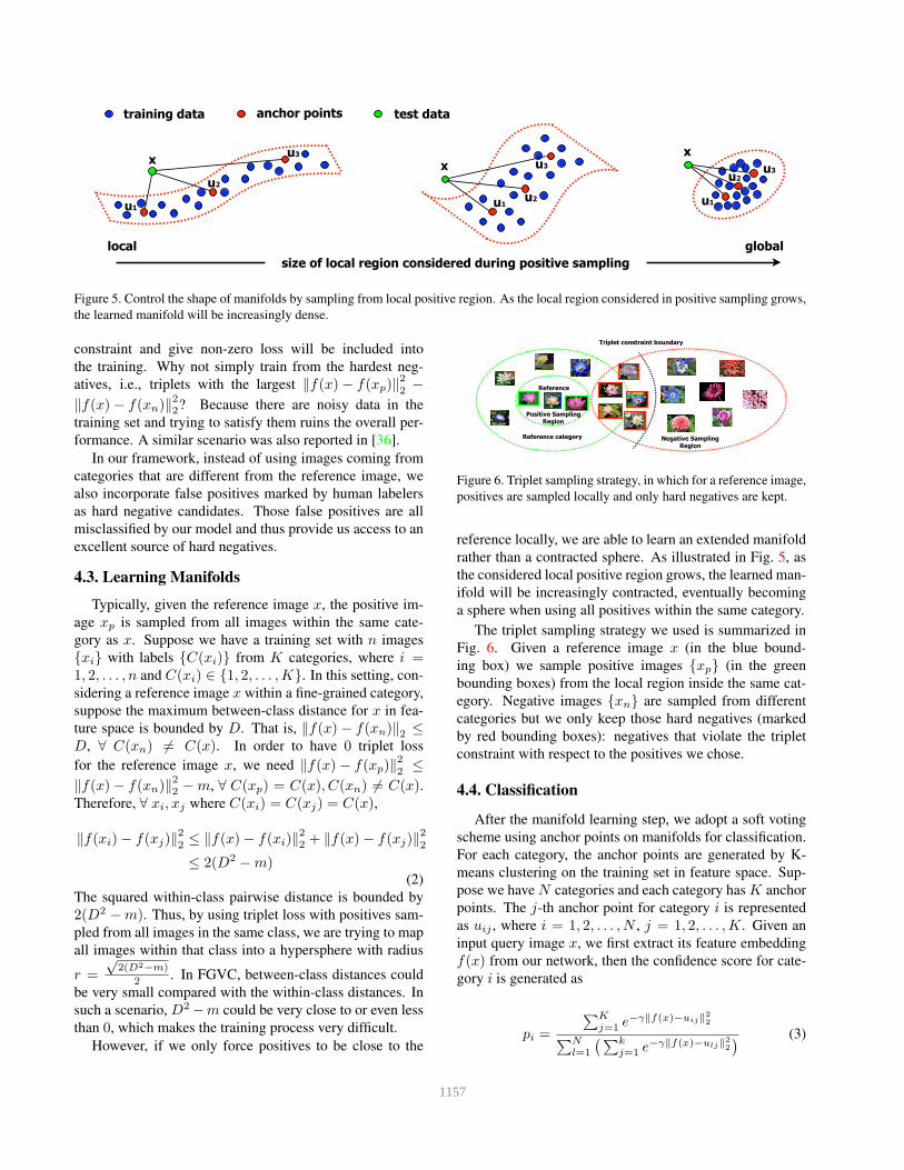
u1u2

u3

u1

u2

u3

u1

u2u3

training data anchor points

size of local region considered during positive sampling

local global

test data

xx

x

Figure 5. Control the shape of manifolds by sampling from local positive region. As the local region considered in positive sampling grows,

the learned manifold will be increasingly dense.

constraint and give non-zero loss will be included into

the training. Why not simply train from the hardest neg-

atives, i.e., triplets with the largest ‖f(x)− f(xp)‖22 −‖f(x)− f(xn)‖22? Because there are noisy data in the

training set and trying to satisfy them ruins the overall per-

formance. A similar scenario was also reported in [36].

In our framework, instead of using images coming from

categories that are different from the reference image, we

also incorporate false positives marked by human labelers

as hard negative candidates. Those false positives are all

misclassified by our model and thus provide us access to an

excellent source of hard negatives.

4.3. Learning Manifolds

Typically, given the reference image x, the positive im-

age xp is sampled from all images within the same cate-

gory as x. Suppose we have a training set with n images

{xi} with labels {C(xi)} from K categories, where i =1, 2, . . . , n and C(xi) ∈ {1, 2, . . . ,K}. In this setting, con-

sidering a reference image x within a fine-grained category,

suppose the maximum between-class distance for x in fea-

ture space is bounded by D. That is, ‖f(x)− f(xn)‖2 ≤D, ∀ C(xn) 6= C(x). In order to have 0 triplet loss

for the reference image x, we need ‖f(x)− f(xp)‖22 ≤‖f(x)− f(xn)‖22 −m, ∀ C(xp) = C(x), C(xn) 6= C(x).Therefore, ∀ xi, xj where C(xi) = C(xj) = C(x),

‖f(xi)− f(xj)‖22 ≤ ‖f(x)− f(xi)‖22 + ‖f(x)− f(xj)‖22≤ 2(D2 −m)

(2)

The squared within-class pairwise distance is bounded by

2(D2 −m). Thus, by using triplet loss with positives sam-

pled from all images in the same class, we are trying to map

all images within that class into a hypersphere with radius

r =

√2(D2−m)

2 . In FGVC, between-class distances could

be very small compared with the within-class distances. In

such a scenario, D2−m could be very close to or even less

than 0, which makes the training process very difficult.

However, if we only force positives to be close to the

Reference

Positive Sampling Region

Negative Sampling Region

Reference category

Triplet constraint boundary

Figure 6. Triplet sampling strategy, in which for a reference image,

positives are sampled locally and only hard negatives are kept.

reference locally, we are able to learn an extended manifold

rather than a contracted sphere. As illustrated in Fig. 5, as

the considered local positive region grows, the learned man-

ifold will be increasingly contracted, eventually becoming

a sphere when using all positives within the same category.

The triplet sampling strategy we used is summarized in

Fig. 6. Given a reference image x (in the blue bound-

ing box) we sample positive images {xp} (in the green

bounding boxes) from the local region inside the same cat-

egory. Negative images {xn} are sampled from different

categories but we only keep those hard negatives (marked

by red bounding boxes): negatives that violate the triplet

constraint with respect to the positives we chose.

4.4. Classification

After the manifold learning step, we adopt a soft voting

scheme using anchor points on manifolds for classification.

For each category, the anchor points are generated by K-

means clustering on the training set in feature space. Sup-

pose we have N categories and each category has K anchor

points. The j-th anchor point for category i is represented

as uij , where i = 1, 2, . . . , N , j = 1, 2, . . . ,K. Given an

input query image x, we first extract its feature embedding

f(x) from our network, then the confidence score for cate-

gory i is generated as

pi =

∑Kj=1 e

−γ‖f(x)−uij‖2

2

∑Nl=1

(∑k

j=1 e−γ‖f(x)−ulj‖

2

2

)(3)

1157

The predicted label of x is the category with the highest

confidence score: argmaxi pi. γ is a parameter controlling

the “softness” of label assignment and closer anchor points

play more significant roles in soft voting. If γ → ∞, only

the nearest anchor point is considered and the predicted la-

bel is “hard” assigned to be the same as the nearest anchor

point. On the other hand, if γ → 0, all the anchor points are

considered to have the same contribution regardless of their

distances between f(x).Notice that during the prediction, the model is pre-

trained offline and all the anchor points are calculated of-

fline. Therefore, given a query image, we only need a sin-

gle forward pass in our model to extract the features. Since

we have learned a low-dimensional embedding, computing

the distances between features and anchor points in low-

dimensional space is very fast.

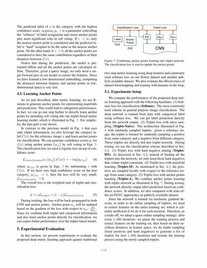
4.5. Learning Anchor Points

As we just described, after metric learning, we use K-

means to generate anchor points for representing manifolds

and prediction. This could lead to suboptimal performance.

In fact, we can go one step further to directly learn anchor

points by including soft voting into our triplet-based metric

learning model, which is illustrated in Fig. 7. For simplic-

ity, the data part is not shown.

In contrast to the previous model in Fig. 4 that uses

only triplet information, we also leverage the category la-

bel C(x) for the reference image x and learn anchor points

for classification. We can generate confidence scores pi for

f(x) using anchor points {uij} by soft voting in Eqn. 3.

The classification loss we used is logistic loss on top of con-

fidence score:

Lclassification(x, {uij}, C(x)) = − log(pC(x)) (4)

where pC(x) is given in Eqn. 3 by substituting i with

C(x). If we have very high confidence score on the true

category, pC(x) → 1, then the loss will be very small:

Lclassification → 0.

The overall loss is the weighted sum of triplet and clas-

sification loss:

L = ωLtriplet + (1− ω)Lclassification (5)

During training, the loss will be back-propagated to both

CNN and anchor points. Anchor point uij will be updated

based on the gradient of the loss with respect to uij : ∂L∂uij

.

Since we combine both triplet and categorical information

and also learn anchor points directly for classification, we

can expect better performance over the triplet-based model.

5. Experimental Evaluation

In this section, we present experiments to evaluate the

proposed deep metric learning approach against traditional

f(x) f(xp) f(xn)

Triplet Loss

CNN

Anchor

Points

Label

Classification Loss

C(x)

{uij}

Figure 7. Combining anchor points learning into triplet network.

The classification loss is used to update the anchor points.

two-step metric learning using deep features and commonly

used softmax loss on our flower dataset and another pub-

licly available dataset. We also evaluate the effectiveness of

dataset bootstrapping and training with humans in the loop.

5.1. Experiments Setup

We compare the performance of the proposed deep met-

ric learning approach with the following baselines: (1) Soft-

max loss for classification (Softmax). The most commonly

used scheme in general purpose image classification. The

deep network is trained from data with categorical label

using softmax loss. We can get label prediction directly

from the network output. (2) Triplet loss with naive sam-

pling (Triplet-Naive). The architecture illustrated in Fig.

4 with randomly sampled triplets: given a reference im-

age, the triplet is formed by randomly sampling a positive

from same category and a negative from different category.

Those triplets are directly fed into triplet network. During

testing, we use the classification scheme described in Sec.

4.4. (3) Triplet loss with hard negative mining (Triplet-

HN). As discussed in Sec. 4.2, instead of feeding all the

triplets into the network, we only keep those hard negatives

that violate triplet constraint. (4) Triplet loss with manifold

learning (Triplet-M). As mentioned in Sec. 4.3, the posi-

tives are sampled locally with respect to the reference im-

age from same category. (5) Triplet loss with anchor points

learning (Triplet-A). We combine anchor points learning

with triplet network as illustrated in Fig. 7. During testing,

the network directly output label prediction based on confi-

dence scores. In addition, we also compared with state-of-

the art FGVC approaches on publicly available dataset.

Since the network is trained via stochastic gradient de-

scent, in order to do online sampling of triplets, we need

to extract features on the entire training set, which is cer-

tainly inefficient if we do it for each iteration. Therefore, as

a trade-off, we adopt a quasi-online sampling strategy: after

every 1, 000 iterations, we pause the training process and

extract features on the training set, then based on their eu-

clidean distances in feature space, we do triplet sampling

(local positives and hard negatives) to generate a list of

triplets for next 1, 000 iterations and resume the training

process using the newly sampled triplets.

1158

The CNN architecture we used is GoogLeNet-Inception

[38], which achieved state-of-the-art performance in large-

scale image classification on ImageNet [12]. All the base-

line models are trained with fine-tuning using pre-trained

GoogleNet-Inception on ImageNet dataset.

We used Caffe [22], an open source deep learning frame-

work, for the implementation and training of our networks.

The models are trained on NVIDIA Tesla K80 GPUs. The

training process typically took about 5 days on a single GPU

to finish 200, 000 iterations with 50 triplets in a batch per

each iteration.

5.2. Deep Metric Learning

We evaluate the baselines on our flower dataset and pub-

licly available CUB-200 Birds dataset [43]. There are sev-

eral parameters in our model and the best values are found

through cross-validation. For all the following experiments

on both dataset, we set the margin m in triplet loss to be

0.2; the feature dimension for f(·) to be 64; the number of

anchor points per each category K to be 3; the γ in soft vot-

ing to be 5. We set ω = 0.1 to make sure that the triplet loss

term and the classification loss term in Eqn. 5 have compa-

rable scale. For the size of positive sampling region, we set

it to be 60% of nearest neighbors within same category. The

effect of positive sampling region size will also be presented

later in this section.

Flowers-620. flowers-620 is the dataset we collected and

used for dataset bootstrapping, which contains 20, 211 im-

ages from 620 flower species, in which 15, 437 images are

used for training. The performance comparison of mean ac-

curacy is summarized in Tab. 1.

Method (feature dimension) Accuracy (%)

Softmax (620) 65.1

Triplet-Naive (64) 48.7

Triplet-HN (64) 64.6

Triplet-M (64) 65.9

Triplet-A (64) 66.8

Table 1. Performance comparison on our flowers-620 dataset.

From the results, we have the following observations: (1)

Triplet-Naive, which uses randomly offline sampling, per-

formed much worse compared with other triplet baselines,

which clearly shows the importance of triplet sampling in

training. (2) Accuracy increases from Triplet-HN to Triplet-

M, showing the effectiveness of learning a better manifolds

with local positive sampling. (3) Triplet-A performed best

and achieved higher accuracy than Softmax. This verifies

our intuition that fine-grained categories often have high

intra-class difference and such within-class variance can be

well captured by learning manifolds with multiple anchor

points. In this way, even in a much lower dimensional fea-

ture space, the discrimination of the data can still be well

preserved. While in Softmax, we are trying to map all the

data within a category to a single point in feature space,

which fails to capture the within-class structure well.

Birds-200. birds-200 is the Caltech-UCSD Birds-200-

2011 data set for fine-grained birds categorization. There

are 11, 788 images from 200 bird species. Each category

has around 30 images for training. In training and testing,

we use the ground truth bounding boxes to crop the images

before feeding them to the network. The performance com-

parison is summarized in Tab. 2.

Method (feature dimension) Accuracy (%)

Alignments [15] 67.0

MsML [35] 67.9

Symbiotic* [8] 69.5

POOF* [5] 73.3

PB R-CNN* [50] 82.0

B-CNN [32] 85.1

PNN* [6] 85.4

Softmax (620) 77.2

Triplet-Naive (64) 61.2

Triplet-HN (64) 77.9

Triplet-M (64) 79.3

Triplet-A (64) 80.7

Table 2. Performance comparison on birds-200 dataset. “*” indi-

cates methods that use ground truth part annotations.

Similar to what we just observed in flowers-620, exper-

iment results verify the effectiveness of proposed methods.

We also compared to recent state-of-the-art approaches for

fine-grained categorization. Notice that we outperformed

MsML [35] by a significant margin, which is a state-of-the-

art metric learning method for FGVC. Although our method

performed worse than the recent proposed B-CNN [32], we

were able to achieve either better or comparable results with

those state-of-the-arts using ground truth part annotations

during training and testing.

We also evaluate the effect of local positive sampling

region size. As we mentioned earlier in Sec. 4.3, the

size of local positive sampling region controls the shape

of manifolds. We want to learn manifolds that can capture

within-class variance well but not too spread out to lose the

between-class discriminations.

Fig. 8 shows the mean accuracy with varying local posi-

tive sampling region using Triplet-M. Using 60% of nearest

neighbors for positive sampling gives best results on both

flowers-620 and birds-200.

5.3. Dataset Bootstrapping

During dataset bootstrapping, other than true positives

that passed human filtering and included into our dataset,

plenty of false positives were marked by human labelers.

Those false positives are perfect hard negatives in our metric

1159

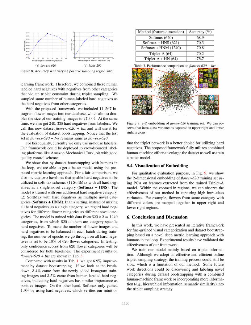
(a) flowers-620 (b) birds-200

Figure 8. Accuracy with varying positive sampling region size.

learning framework. Therefore, we combined these human

labeled hard negatives with negatives from other categories

that violate triplet constraint during triplet sampling. We

sampled same number of human-labeled hard negatives as

the hard negatives from other categories.

With the proposed framework, we included 11, 567 In-

stagram flower images into our database, which almost dou-

bles the size of our training images to 27, 004. At the same

time, we also get 240, 338 hard negatives from labelers. We

call this new dataset flowers-620 + Ins and will use it for

the evaluation of dataset bootstrapping. Notice that the test

set in flowers-620 + Ins remains same as flowers-620.

For best quality, currently we only use in-house labelers.

Our framework could be deployed to crowdsourced label-

ing platforms like Amazon Mechanical Turk, bit with good

quality control schemes.

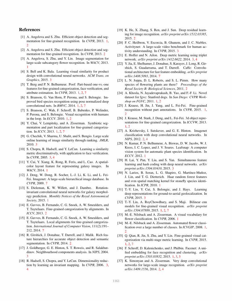
We show that by dataset bootstrapping with humans in

the loop, we are able to get a better model using the pro-

posed metric learning approach. For a fair comparison, we

also include two baselines that enable hard negatives to be

utilized in softmax scheme: (1) SoftMax with all hard neg-

atives as a single novel category (Softmax + HNS). The

model is trained with one additional hard negative category.

(2) SoftMax with hard negatives as multiple novel cate-

gories (Softmax + HNM). In this setting, instead of mixing

all hard negatives as a single category, we regard hard neg-

atives for different flower categories as different novel cate-

gories. The model is trained with data from 620×2 = 1240categories, from which 620 of them are category-specific

hard negatives. To make the number of flower images and

hard negatives to be balanced in each batch during train-

ing, the number of epochs we go through on all hard nega-

tives is set to be 10% of 620 flower categories. In testing,

only confidence scores from 620 flower categories will be

considered for both baselines. The experiment results on

flowers-620 + Ins are shown in Tab. 3.

Compared with results in Tab. 1, we got 6.9% improve-

ment by dataset bootstrapping. If we look at the break-

down, 3.4% came from the newly added Instagram train-

ing images and 3.5% came from human labeled hard neg-

atives, indicating hard negatives has similar importance as

positive images. On the other hand, Softmax only gained

1.9% by using hard negatives, which verifies our intuition

Method (feature dimension) Accuracy (%)

Softmax (620) 68.9

Softmax + HNS (621) 70.3

Softmax + HNM (1240) 70.8

Triplet-A (64) 70.2

Triplet-A + HN (64) 73.7

Table 3. Performance comparison on flowers-620 + Ins.

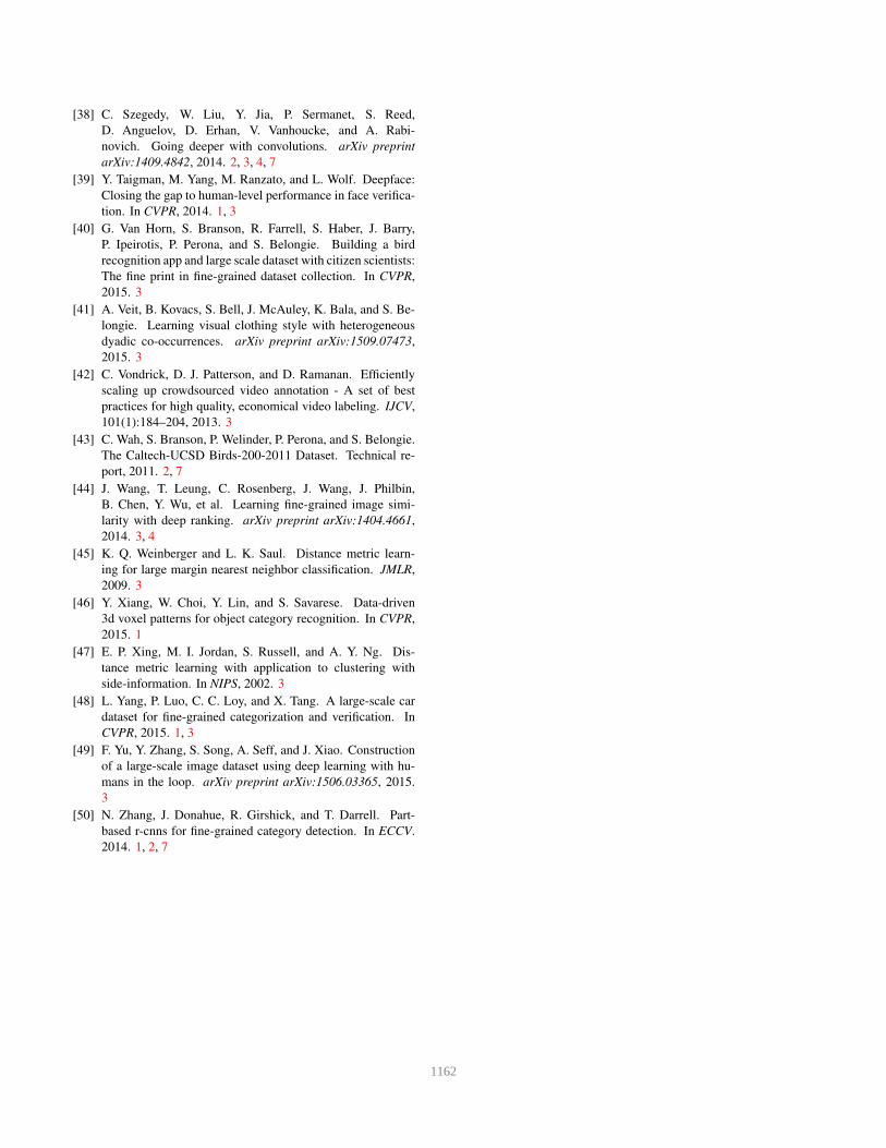
Figure 9. 2-D embedding of flower-620 training set. We can ob-

serve that intra-class variance is captured in upper right and lower

right regions.

that the triplet network is a better choice for utilizing hard

negatives. The proposed framework fully utilizes combined

human-machine efforts to enlarge the dataset as well as train

a better model.

5.4. Visualization of Embedding

For qualitative evaluation purpose, in Fig. 9, we show

the 2-dimensional embedding of flower-620 training set us-

ing PCA on features extracted from the trained Triplet-A

model. Within the zoomed in regions, we can observe the

effectiveness of our method in capturing high intra-class

variances. For example, flowers from same category with

different colors are mapped together in upper right and

lower right regions.

6. Conclusion and Discussion

In this work, we have presented an iterative framework

for fine-grained visual categorization and dataset bootstrap-

ping based on a novel deep metric learning approach with

humans in the loop. Experimental results have validated the

effectiveness of our framework.

We train our model mainly based on triplet informa-

tion. Although we adopt an effective and efficient online

triplet sampling strategy, the training process could still be

slow, which is a limitation of our method. Some future

work directions could be discovering and labeling novel

categories during dataset bootstrapping with a combined

human-machine framework or incorporating more informa-

tion (e.g., hierarchical information, semantic similarity) into

the triplet sampling strategy.

1160

References

[1] A. Angelova and S. Zhu. Efficient object detection and seg-

mentation for fine-grained recognition. In CVPR, 2013. 1,

2

[2] A. Angelova and S. Zhu. Efficient object detection and seg-

mentation for fine-grained recognition. In CVPR, 2013. 2

[3] A. Angelova, S. Zhu, and Y. Lin. Image segmentation for

large-scale subcategory flower recognition. In WACV, 2013.

1

[4] S. Bell and K. Bala. Learning visual similarity for product

design with convolutional neural networks. ACM Trans. on

Graphics, 2015. 3

[5] T. Berg and P. N. Belhumeur. Poof: Part-based one-vs.-one

features for fine-grained categorization, face verification, and

attribute estimation. In CVPR, 2013. 1, 2, 7

[6] S. Branson, G. Van Horn, P. Perona, and S. Belongie. Im-

proved bird species recognition using pose normalized deep

convolutional nets. In BMVC, 2014. 1, 2, 7

[7] S. Branson, C. Wah, F. Schroff, B. Babenko, P. Welinder,

P. Perona, and S. Belongie. Visual recognition with humans

in the loop. In ECCV. 2010. 1, 2

[8] Y. Chai, V. Lempitsky, and A. Zisserman. Symbiotic seg-

mentation and part localization for fine-grained categoriza-

tion. In ICCV, 2013. 1, 2, 7

[9] G. Chechik, V. Sharma, U. Shalit, and S. Bengio. Large scale

online learning of image similarity through ranking. JMLR,

2010. 3

[10] S. Chopra, R. Hadsell, and Y. LeCun. Learning a similarity

metric discriminatively, with application to face verification.

In CVPR, 2005. 3, 4

[11] Y. Cui, Y. Xiang, K. Rong, R. Feris, and L. Cao. A spatial-

color layout feature for representing galaxy images. In

WACV, 2014. 1

[12] J. Deng, W. Dong, R. Socher, L.-J. Li, K. Li, and L. Fei-

Fei. Imagenet: A large-scale hierarchical image database. In

CVPR, 2009. 7

[13] S. Dieleman, K. W. Willett, and J. Dambre. Rotation-

invariant convolutional neural networks for galaxy morphol-

ogy prediction. Monthly Notices of the Royal Astronomical

Society, 2015. 1

[14] E. Gavves, B. Fernando, C. G. Snoek, A. W. Smeulders, and

T. Tuytelaars. Fine-grained categorization by alignments. In

ICCV, 2013. 2

[15] E. Gavves, B. Fernando, C. G. Snoek, A. W. Smeulders, and

T. Tuytelaars. Local alignments for fine-grained categoriza-

tion. International Journal of Computer Vision, 111(2):191–

212, 2014. 7

[16] R. Girshick, J. Donahue, T. Darrell, and J. Malik. Rich fea-

ture hierarchies for accurate object detection and semantic

segmentation. In CVPR, 2014. 2

[17] J. Goldberger, G. E. Hinton, S. T. Roweis, and R. Salakhut-

dinov. Neighbourhood components analysis. In NIPS, 2004.

3

[18] R. Hadsell, S. Chopra, and Y. LeCun. Dimensionality reduc-

tion by learning an invariant mapping. In CVPR, 2006. 3,

4

[19] K. He, X. Zhang, S. Ren, and J. Sun. Deep residual learn-

ing for image recognition. arXiv preprint arXiv:1512.03385,

2015. 2

[20] F. C. Heilbron, V. Escorcia, B. Ghanem, and J. C. Niebles.

Activitynet: A large-scale video benchmark for human ac-

tivity understanding. In CVPR, 2015. 3

[21] E. Hoffer and N. Ailon. Deep metric learning using triplet

network. arXiv preprint arXiv:1412.6622, 2014. 3, 4

[22] Y. Jia, E. Shelhamer, J. Donahue, S. Karayev, J. Long, R. Gir-

shick, S. Guadarrama, and T. Darrell. Caffe: Convolu-

tional architecture for fast feature embedding. arXiv preprint

arXiv:1408.5093, 2014. 7

[23] L. N. Joppa, D. L. Roberts, and S. L. Pimm. How many

species of flowering plants are there? Proceedings of the

Royal Society B: Biological Sciences, 2011. 2

[24] A. Khosla, N. Jayadevaprakash, B. Yao, and F.-F. Li. Novel

dataset for fgvc: Stanford dogs. In San Diego: CVPR Work-

shop on FGVC, 2011. 1, 2

[25] J. Krause, H. Jin, J. Yang, and L. Fei-Fei. Fine-grained

recognition without part annotations. In CVPR, 2015. 1,

2

[26] J. Krause, M. Stark, J. Deng, and L. Fei-Fei. 3d object repre-

sentations for fine-grained categorization. In ICCVW, 2013.

1, 2

[27] A. Krizhevsky, I. Sutskever, and G. E. Hinton. Imagenet

classification with deep convolutional neural networks. In

NIPS, 2012. 2, 4

[28] N. Kumar, P. N. Belhumeur, A. Biswas, D. W. Jacobs, W. J.

Kress, I. C. Lopez, and J. V. Soares. Leafsnap: A computer

vision system for automatic plant species identification. In

ECCV. 2012. 1

[29] H. Lai, Y. Pan, Y. Liu, and S. Yan. Simultaneous feature

learning and hash coding with deep neural networks. arXiv

preprint arXiv:1504.03410, 2015. 3

[30] N. Larios, B. Soran, L. G. Shapiro, G. Martınez-Munoz,

J. Lin, and T. G. Dietterich. Haar random forest features

and svm spatial matching kernel for stonefly species identi-

fication. In ICPR, 2010. 1

[31] T.-Y. Lin, Y. Cui, S. Belongie, and J. Hays. Learning

deep representations for ground-to-aerial geolocalization. In

CVPR, 2015. 3

[32] T.-Y. Lin, A. RoyChowdhury, and S. Maji. Bilinear cnn

models for fine-grained visual recognition. arXiv preprint

arXiv:1504.07889, 2015. 1, 2, 7

[33] M.-E. Nilsback and A. Zisserman. A visual vocabulary for

flower classification. In CVPR, 2006. 1

[34] M.-E. Nilsback and A. Zisserman. Automated flower classi-

fication over a large number of classes. In ICVGIP, 2008. 1,

2

[35] Q. Qian, R. Jin, S. Zhu, and Y. Lin. Fine-grained visual cat-

egorization via multi-stage metric learning. In CVPR, 2015.

1, 2, 7

[36] F. Schroff, D. Kalenichenko, and J. Philbin. Facenet: A uni-

fied embedding for face recognition and clustering. arXiv

preprint arXiv:1503.03832, 2015. 1, 3, 5

[37] K. Simonyan and A. Zisserman. Very deep convolutional

networks for large-scale image recognition. arXiv preprint

arXiv:1409.1556, 2014. 2, 4

1161

[38] C. Szegedy, W. Liu, Y. Jia, P. Sermanet, S. Reed,

D. Anguelov, D. Erhan, V. Vanhoucke, and A. Rabi-

novich. Going deeper with convolutions. arXiv preprint

arXiv:1409.4842, 2014. 2, 3, 4, 7

[39] Y. Taigman, M. Yang, M. Ranzato, and L. Wolf. Deepface:

Closing the gap to human-level performance in face verifica-

tion. In CVPR, 2014. 1, 3

[40] G. Van Horn, S. Branson, R. Farrell, S. Haber, J. Barry,

P. Ipeirotis, P. Perona, and S. Belongie. Building a bird

recognition app and large scale dataset with citizen scientists:

The fine print in fine-grained dataset collection. In CVPR,

2015. 3

[41] A. Veit, B. Kovacs, S. Bell, J. McAuley, K. Bala, and S. Be-

longie. Learning visual clothing style with heterogeneous

dyadic co-occurrences. arXiv preprint arXiv:1509.07473,

2015. 3

[42] C. Vondrick, D. J. Patterson, and D. Ramanan. Efficiently

scaling up crowdsourced video annotation - A set of best

practices for high quality, economical video labeling. IJCV,

101(1):184–204, 2013. 3

[43] C. Wah, S. Branson, P. Welinder, P. Perona, and S. Belongie.

The Caltech-UCSD Birds-200-2011 Dataset. Technical re-

port, 2011. 2, 7

[44] J. Wang, T. Leung, C. Rosenberg, J. Wang, J. Philbin,

B. Chen, Y. Wu, et al. Learning fine-grained image simi-

larity with deep ranking. arXiv preprint arXiv:1404.4661,

2014. 3, 4

[45] K. Q. Weinberger and L. K. Saul. Distance metric learn-

ing for large margin nearest neighbor classification. JMLR,

2009. 3

[46] Y. Xiang, W. Choi, Y. Lin, and S. Savarese. Data-driven

3d voxel patterns for object category recognition. In CVPR,

2015. 1

[47] E. P. Xing, M. I. Jordan, S. Russell, and A. Y. Ng. Dis-

tance metric learning with application to clustering with

side-information. In NIPS, 2002. 3

[48] L. Yang, P. Luo, C. C. Loy, and X. Tang. A large-scale car

dataset for fine-grained categorization and verification. In

CVPR, 2015. 1, 3

[49] F. Yu, Y. Zhang, S. Song, A. Seff, and J. Xiao. Construction

of a large-scale image dataset using deep learning with hu-

mans in the loop. arXiv preprint arXiv:1506.03365, 2015.

3

[50] N. Zhang, J. Donahue, R. Girshick, and T. Darrell. Part-

based r-cnns for fine-grained category detection. In ECCV.

2014. 1, 2, 7

1162