Embed Size (px)
Citation preview

Finite Buffer Queueing/Fluid Networkswith Overflows
Erjen Lefeber, Yoni Nazarathy.
Swinburne Applied Mathematics Seminar,
April Fools’ Day, 2011.
* Supported by NWO-VIDI Grant 639.072.072

Background Jackson Networks and LCP

Open Jackson NetworksJackson 1957, Goodman & Massey 1984, Chen & Mandelbaum 1991
1
1
'( ')
M
i i j j ij
p
PI P
λ α λ
λ α λ
λ α
=
−
= +
= +
= −
∑
, ,M M M MPµ α ×
( )( )
( )
1
'
( ') , ( ')
M
i i j j j ij
p
P
LCP I P I P
λ α λ µ
λ α λ µ
α µ
=
= + ∧
= + ∧
− − −
∑
iµiα
Traffic Equations (Stable Case):
Traffic Equations (General Case):
i jp
1µ
Mµ
11
M
i jij
p p=
= −∑
Problem Data:
Assume: open, no “dead” nodes

The Linear Complementarity Problem (LCP)
The last (complemenatrity) condition reads:0 0 and 0 0.i i i iw z z w> ⇒ = > ⇒ =

Min-Linear Equations (Using LCP)( )Bλ γ λ µ= + ∧
00( ) '( ) 0
Bλ γ δδ λδ µ
λ δ µ δ
= +≤ ≤≤ ≤− − =
,w zλ δ µ δ= − = −
( ( ) , )LCP I B I Bγ µ− − −
δ λ µ= ∧Find :λ

Classic Product Form Results Jackson 1957, Goodman & Massey 1984
( )( )
( )
1
'
( ') , ( ')
M
i i j j j ij
p
P
LCP I P I P
λ α λ µ
λ α λ µ
α µ
=
= + ∧
= + ∧
− − −
∑
Assume arrivals are Poisson processes and i.i.d. exponential service durations
Again the Traffic Equations :

Our Contribution:Finite Buffers with Overflows

Modification: Finite Buffers and Overflows Practically important but not as tractable
iµiαExact Traffic Equations:i jp
Mµ
11
M
i jij
p p=
= −∑
Problem Data:
, , , ,M M M M M M MP K Qµ α × ×
Explicit Solutions:
Generally NoiK
MK1
1M
i jij
q q=
= −∑
i jq
1µ1K
Generally No
Assume: open, no “dead” nodes, no “jam” (open overflows)
Nico van Dijk, 1988. Yes if P=Q.

So scale the system with :
When K is Big, Things are “Simpler”
out rate λ µ≈ ∧overflow rate ( )λ λ µ λ µ +≈ − ∧ = −
N
N
N
NN K
α α
µ µ
= Ν
=
Κ =
1,2,...N =
For K big:
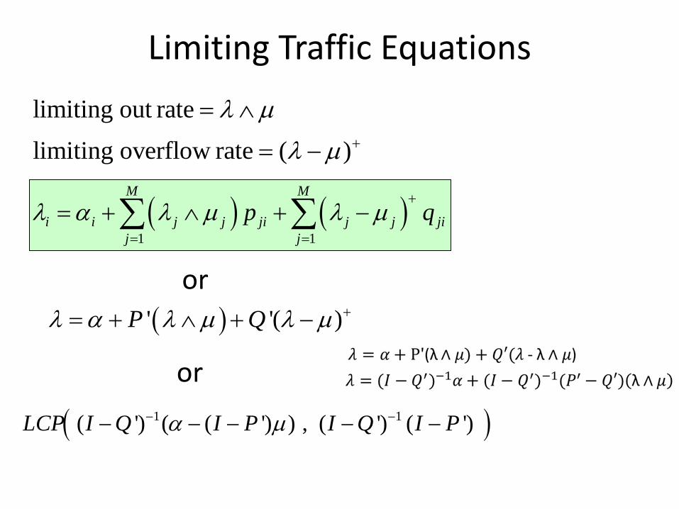
Limiting Traffic Equations
( ) ( )1 1
M M
i i j j ji j j jij j
p qλ α λ µ λ µ+
= =
= + ∧ + −∑ ∑
limiting out rate λ µ= ∧
limiting overflow rate ( )λ µ += −
( )' '( )P Qλ α λ µ λ µ += + ∧ + −
or
( )1 1( ') ( ( ') ) , ( ') ( ')LCP I Q I P I Q I Pα µ− −− − − − −
or

Digression:The Linear Complementarity Problem (LCP)

The Linear Complementarity Problem (LCP)
The last (complemenatrity) condition reads:0 0 and 0 0.i i i iw z z w> ⇒ = > ⇒ =

It’s all about Choosing a Subset…For {1,..., } denote by ( ) a matrix withcollumns taken from (identity matrix)and collumns {1,..., } \ taken from .
n BI
n M
α αα
α
⊆
−
is about finding and 0such that
( )In this case:
LCP x
B x q
α
α
≥
=
0, .
0i
i ii
ix iw z
x iiαααα
∈∈ = = ∉∉

Illustration: n=2
1 0 11 20 1 2
1 12 11 20 22 2
011 11 2121 2
11 12 11 2
21 22 2
{1,2}:
{1}:
{2}:
:
qw w
q
m qw z
m q
m qz w
m q
m m qz z
m m q
α
α
α
α
+ =
− + = −
− + = −
− − + = − −
=
=
=
=∅
1 11 12 1 1
2 21 22 2 2
1 00 1
w m m z qw m m z q
− =
{1,2}C
Complementary cones:
10
01
12
22
mm
− −
11
21
mm
− −
1
2
{1}C
{2}C
{ : ( ) , 0}C y y B u uα α= = ≥
C∅
Immediate naïve algorithm with complexity 3 32 2n nn or n+

Existence and UniquenessDefinition: A matrix, is a P-matrix if thedeterminants of all (2 1) principal submatrices are positive.
n n
n
M ×∈
−
Theorem (1958): ( , ) has a unique solutionfor all if and only if is a P-matrix.n
LCP q Mq M∈
11 22 11 22 12 21e.g.for 2 : 0, 0, 0n m m m m m m= > > − >
P-matrix means that the complementary cones "parition" n
P-Matrixes
Symmetric MatrixesPD Matrixes
Relation of P-matrixes to positive definite (PD) matrixes:
Reminder(PD) :' 0 0x Mx x> ∀ ≠
Reminder(PSD) :' 0x Mx x≥ ∀

Computation (Algorithms)• Naive algorithm, runs on all subsets alpha (intractable)• Generally, LCP is NP complete• Lemeke’s Algorithm, a bit like simplex• If M is PSD: polynomial time algorithms exists• PD LCP equivalent to QP• Special cases of M, linear number of iterations• Note: Checking for P-Matrix is NP complete, checking for PD is
polynomial time• For our special case we have an algorithm with a quadratic
number of iterations(Still have not done: proven uniqueness using LCP theory).

How does LCP generalize LP and QP?

Linear Programming (LP)
min '. .
0
c xs t Ax b
x≥≥
max '. . '
0
b ys t A y c
y≤≥
Primal-LP: Dual-LP:
Theorem: Complementary slackness conditions
min '. .
, 0
c xs t Ax b v
x v− =≥
max '. . '
, 0
b ys t u c A y
y u= −
≥
Assume , , , are feasible for primaland dual:0, 0 Theyareoptimalsolutionsi i i i
x v y ux u y v= = ⇔

0 ',
0c A
LCPb A
− −
0 '0
u A x cv A y b
− − = −
, , , 0u v x y ≥
' 0u x = ' 0v y =
The LCP of LPFind:
Such that:
And (complementary slackness):

Quadratic Programming1min ( ) ' '2
. .0
Q x c x x D x
s t Ax bx
= +
≥≥
Lemma: An optimizer, , of the QP also optimizes min ( ) '. .
0
c Dx xs t Ax b
x
+≥≥
Proof:( )x x x xη η= + −
( ) ( ) 0Q x Q xη − ≥ ( ' ) '( ) ( ) ' ( )
2c Dx x x x x D x xη−+ − ≥ − −
x
QP-LP:
QP-LP gives a necessary condition for optimality of QP in terms of an checking optimality of an LP
QP:
0 1,η< <Let be feasible.x
( ' ) '( ) 0c Dx x x+ − ≥
( ' ) ' ( ' ) 'c Dx x c Dx x+ ≥ +

The Resulting LCP of QP
',
0c D A
LCPb A
− −
Allows to find “suspect” points that satisfy the necessary conditions: QP-LP
Theorem: Solutions of this LCP are KKT (Karush-Kuhn-Tucker) points for the QP
Corollary: If D is PSD then x solving the LCP optimizes QP.
Proof: Write down KKT conditions and check.
Note: When D is PSD then M is PSD. In this case it can be shown that the LCP is equivalent to a QP (solved in polynomial time). Similarly, every PSD LCP can be formulated as a PSD QP.

Back To Our Problem:The Fluid Network

Limiting TrajectoriesIn similar spirit to the traffic equations, limiting trajectories, , may be calculated…
( )lim sup ( ) 0N
tN
X t x tN→∞
− =
( )x t
a.s.
We think:

Sojourn Times
Sojourn Time Time in system of customer arriving to steady state FCFS system
≡
Sojourn time of customer in 'th scaled systemNS N≡
We want to find the limiting distribution of NS

Construction of Limiting Sojourn Times
time through i F i
i
Kµ
∈ ≈
{1,..., }
{ 1,..., }
F s
F s M
=
= +
i i
i i
for i S
for i S
λ µ
λ µ
> ∈
< ∈Observe,
time through i F 0∈ ≈For job at entrance of buffer :
. . enters buffer i
. . 1 routed to entrace of buffer j
. . 1 leaves the system
i
i
iij
i
ii
i
w p
w p q
w p q
µλ
µλ
µλ
≈
≈ −
≈ −
i F∈
A “fast” chain and “slow” chain…
A job at entrance of buffer : routed almost immediately according toi F∈ P

Sojourn Times Scale to a Discrete Distribution!!!
We think: ( )1,Ns s sS DPH T τ× ×⇒1,i
i
K i Fµ = ∈
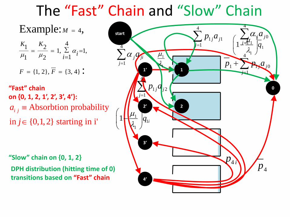
The “Fast” Chain and “Slow” Chain
1’
2’
3’
4’
1
2
0
4
41 2 1, 1,11 2
{1, 2}, {3, 4}
Example: ,
:
M
K Kii
F F
αµ µ
=
∑= = ==
= =
11
1
1 iqµλ
−
4p
4
1 011
j jj
p p a=
+∑
4
1 11
j jj
p a=∑
Absorbtion probability
in {0,1,2} starting in i'i ja
j
≡
∈
“Fast” chain on {0, 1, 2, 1’, 2’, 3’, 4’}:
“Slow” chain on {0, 1, 2}
start
4
1 21
j jj
p a=∑
1
1
µλ
11
1
1 qµλ
−
4 ip
4
1j ji
jaα
=∑
4
01
j jj
aα=∑
DPH distribution (hitting time of 0)transitions based on “Fast” chain

The DPH Parameters (Details)
1~ ( , )s s sS DPH T τ× ×
{1,..., }, { 1,..., }F s F s M= = +
1P( ) 1 1ksS k Tτ ×≤ = − ⋅ ⋅
1
1
1
00 0
1
0
s M sM M M M s M s
s M s
s
M s s
C Q PI
µλ
µλ
× −× × − ×
−
− ×
−
= ⋅ + ⋅ −
1
10
0
0
M ss
s
M s s
B
µλ
µλ
×
− ×
=
1( )M sA I C B−× = − ⋅
0s s s s M sT I P A× × − = ⋅ ⋅ 1
1
1 Ts M
jj
Aτ αα
×
=
= ⋅
∑
“Fast” chain
“Slow” chain

Mechanism of nonlinear flow pattern selection in moderately non-Boussinesq mixed convection
Yoni Nazarathy, Sergey Suslov,
John Beynon, William Phillips
Swinburne Applied Mathematics Seminar,
April 1, 2011.