Embed Size (px)
Citation preview
Finite Difference Computingwith PDEs - A Modern Software
Approach
Hans Petter Langtangen1,2
Svein Linge3,1
1Center for Biomedical Computing, Simula Research Laboratory2Department of Informatics, University of Oslo
3Department of Process, Energy and Environmental Technology,University College of Southeast Norway
This easy-to-read book introduces the basics of solving partial dif-ferential equations by finite difference methods. The emphasis ison constructing finite difference schemes, formulating algorithms,implementing algorithms, verifying implementations, analyzing thephysical behavior of the numerical solutions, and applying the meth-ods and software to solve problems from physics and biology.
iv
Oct 1, 2016
Preface
There are so many excellent books on finite difference methods forordinary and partial differential equations that writing yet another onerequires a different view on the topic. The present book is not so concernedwith the traditional academic presentation of the topic, but is focused atteaching the practitioner how to obtain reliable computations involvingfinite difference methods. This focus is based on a set of learning outcomes:
1. understanding of the ideas behind finite difference methods,2. understanding how to transform an algorithm to a well-designed
computer code,3. understanding how to test (verify) the code,4. understanding potential artifacts in simulation results.
Compared to other textbooks, the present one has a particularly strongemphasis on computer implementation and verification. It also has astrong emphasis on an intuitive understanding of constructing finitedifference methods. To learn about the potential non-physical artifactsof various methods, we study exact solutions of finite difference schemesas these give deeper insight into the physical behavior of the numericalmethods than the traditional (and more general) asymptotic error analy-sis. However, asymptotic results regarding convergence rates, typicallytruncation errors, are crucial for testing implementations, so an extensiveappendix is devoted to the computation of truncation errors.
Why finite differences? One may ask why we do finite differences whenfinite element and finite volume methods have been developed to greater
© 2016, Hans Petter Langtangen, Svein Linge. Released under CC Attribution 4.0 license
vi
generality and sophistication than finite differences and can cover moreproblems. The finite element and finite volume methods are also theindustry standard nowadays. Why not just those methods? The reasonfor finite differences is the method’s simplicity, both from a mathematicaland coding perspective. Especially in academia, where simple modelproblems are used a lot for teaching and in research (e.g., for verificationof advanced implementations), there is a constant need to solve the modelproblems from scratch with easy-to-verify computer codes. Here, finitedifferences are ideal. A simple 1D heat equation can of course be solvedby a finite element package, but a 20-line code with a difference schemeis just right to the point and provides an understanding of all detailsinvolved in the model and the solution method. Everybody nowadays hasa laptop and the natural method to attack a 1D heat equation is a simplePython or Matlab program with a difference scheme. The conclusiongoes for other fundamental PDEs like the wave equation and Poissonequation as long as the geometry of the domain is a hypercube. Thepresent book contains all the practical information needed to use thefinite difference tool in a safe way.
Various pedagogical elements are utilized to reach the learning out-comes, and these are commented upon next.Simplify, understand, generalize. The book’s overall pedagogical phi-losophy is the three-step process of first simplifying the problem tosomething we can understand in detail, and when that understanding isin place, we can generalize and hopefully address real-world applicationswith a sound scientific problem-solving approach. For example, in thechapter on a particular family of equations we first simplify the problemin question to a 1D, constant-coefficient equation with simple boundaryconditions. We learn how to construct a finite difference method, how toimplement it, and how to understand the behavior of the numerical solu-tion. Then we can generalize to higher dimensions, variable coefficients,a source term, and more complicated boundary conditions. The solutionof a compound problem is in this way an assembly of elements that arewell understood in simpler settings.Constructive mathematics. This text favors a constructive approachto mathematics. Instead of a set of definitions followed by popping up amethod, we emphasize how to think about the construction of a method.The aim is to obtain a good intuitive understanding of the mathematicalmethods.
The text is written in an easy-to-read style much inspired by thefollowing quote.
vii
Some people think that stiff challenges are the best device to induce learning, butI am not one of them. The natural way to learn something is by spending vastamounts of easy, enjoyable time at it. This goes whether you want to speak German,sight-read at the piano, type, or do mathematics. Give me the German storybookfor fifth graders that I feel like reading in bed, not Goethe and a dictionary. Thelatter will bring rapid progress at first, then exhaustion and failure to resolve.The main thing to be said for stiff challenges is that inevitably we will encounterthem, so we had better learn to face them boldly. Putting them in the curriculumcan help teach us to do so. But for teaching the skill or subject matter itself, theyare overrated. [18, p. 86] Lloyd N. Trefethen, Applied Mathematician, 1955-.
This book assumes some basic knowledge of finite difference approxi-mations, differential equations, and scientific Python or MATLAB pro-gramming, as often met in an introductory numerical methods course.Readers without this background may start with the light companionbook “Finite Difference Computing with Exponential Decay Models” [9].That book will in particular be a useful resource for the programmingparts of the present book. Since the present book deals with partialdifferential equations, the reader is assumed to master multi-variablecalculus and linear algebra.
Fundamental ideas and their associated scientific details are firstintroduced in the simplest possible differential equation setting, often anordinary differential equation, but in a way that easily allows reuse in morecomplex settings with partial differential equations. With this approach,new concepts are introduced with a minimum of mathematical details.The text should therefore have a potential for use early in undergraduatestudent programs.All nuts and bolts. Many have experienced that “vast amounts of easy,enjoyable time”, as stated in the quote above, arises when mathematicsis implemented on a computer. The implementation process triggersunderstanding, creativity, and curiosity, but many students find thetransition from a mathematical algorithm to a working code difficult andspend a lot of time on “programming issues”.
Most books on numerical methods concentrate on the mathematics ofthe subject while details on going from the mathematics to a computerimplementation are less in focus. A major purpose of this text is thereforeto help the practitioner by providing all nuts and bolts necessary forsafely going from the mathematics to a well-designed and well-testedcomputer code. A significant portion of the text is consequently devotedto programming details.Python as programming language. While MATLAB enjoys widespreadpopularity in books on numerical methods, we have chosen to use the
viii
Python programming language. Python is very similar to MATLAB, butcontains a lot of modern software engineering tools that have becomestandard in the software industry and that should be adopted also fornumerical computing projects. Python is at present also experiencingan exponential growth in popularity within the scientific computingcommunity. One of the book’s goals is to present an up-to-date Pythoneco system for implementing finite difference methods.
Program verification. Program testing, called verification, is a keytopic of the book. Good verification techniques are indispensable whendebugging computer code, but also fundamental for achieving reliablesimulations. Two verification techniques saturate the book: exact solutionof discrete equations (where the approximation error vanishes) and em-pirical estimation of convergence rates in problems with exact (analyticalor manufactured) solutions of the differential equation(s).
Vectorized code. Finite difference methods lead to code with loopsover large arrays. Such code in plain Python is known to run slowly.We demonstrate, especially in Appendix C, how to port loops to fast,compiled code in C or Fortran. However, an alternative is to vectorizethe code to get rid of explicit Python loops, and this technique is metthroughout the book. Vectorization becomes closely connected to theunderlying array library, here numpy, and is often thought of as a difficultsubject by students. Through numerous examples in different contexts,we hope that the present book provides a substantial contribution toexplaining how algorithms can be vectorized. Not only will this speed upserial code, but with a library that can produce parallel code from numpycommands (such as Numba1), vectorized code can be automaticallyturned into parallel code and utilize multi-core processors and GPUs.Also when creating tailored parallel code for today’s supercomputers,vectorization is useful as it emphasizes splitting up an algorithm intoplain and simple array operations, where each operation is trivial toparallelize efficiently, rather than trying to develop a “smart” overallparallelization strategy.
Analysis via exact solutions of discrete equations. Traditional asymp-totic analysis of errors is important for verification of code using con-vergence rates, but gives a limited understanding of how and why acorrectly implemented numerical method may give non-physical results.By developing exact solutions, usually based on Fourier methods, of
1 http://numba.pydata.org
ix
the discrete equations, one can obtain a physical understanding of thebehavior of a numerical method. This approach is favored for analysis ofmethods in this book.Code-inspired mathematical notation. Our primary aim is to have aclean and easy-to-read computer code, and we want a close one-to-onerelationship between the computer code and mathematical descriptionof the algorithm. This principle calls for a mathematical notation that isgoverned by the natural notation in the computer code. The unknown ismostly called u, but the meaning of the symbol u in the mathematicaldescription changes as we go from the exact solution fulfilling the differ-ential equation to the symbol u that is naturally used for the associateddata structure in the code.Limited scope. The aim of this book is not to give an overview of a lotof methods for a wide range of mathematical models. Such informationcan be found in numerous existing, more advanced books. The aim israther to introduce basic concepts and a thorough understanding of howto think about computing with finite difference methods. We thereforego in depth with only the most fundamental methods and equations.However, we have a multi-disciplinary scope and address the interplay ofmathematics, numerics, computer science, and physics.Focus on wave phenomena. Most books on finite difference methods,or books on theory with computer examples, have their emphasis ondiffusion phenomena. Half of this book (Chapters 1, 2, and Appendix C)is devoted to wave phenomena. Extended material on this topic is not soeasy find in the literature, so the book should be a valuable contributionin this respect. Wave phenomena is also a good topic in general forchoosing the finite difference method over other discretization methodssince one quickly needs fine resolution over the entire mesh and uniformmeshes are most natural.
Instead of introducing the finite difference method for diffusion prob-lems, where one soon ends up with matrix systems, we do the introductionin a wave phenomena setting where explicit schemes are most relevant.This slows down the learning curve since we can introduce a lot of theoryfor differences and for software aspects in a context with simple, explicitstencils for updating the solution.Independent chapters. Most book authors are careful with avoidingrepetitions of material. The chapters in this book, however, contain someoverlap, because we want the chapters to appear meaningful on their own.Modern publishing technology makes it easy to take selected chapters
x
from different books to make a new book tailored to a specific course. Themore a chapter builds on details in other chapters, the more difficult it isto reuse chapters in new contexts. Also, most readers find it convenientthat important information is explicitly stated, even if it was alreadymet in another chapter.
Supplementary materials. All program and data files referred to inthis book are available from the book’s primary web site: URL: http://hplgit.github.io/fdm-book/doc/web/.
Acknowledgments. Many students have provided lots of useful feedbackon the exposition and found many errors in the text. Special efforts inthis regard were made by Imran Ali, Shirin Fallahi, Anders Hafreager,Daniel Alexander Mo Søreide Houshmand, Kristian Gregorius Hustad,Mathilde Nygaard Kamperud, and Fatemeh Miri. The collaboration withthe Springer team, with Dr. Martin Peters, Thanh-Ha Le Thi, and theirproduction staff has always been a great pleasure and a very efficientprocess.
Finally, want really appreciate the strong push of the COE of SimulaResearch Laboratory, Aslak Tveito, for publishing and financing booksin open access format, including this one. We are grateful to the labo-ratory’s financial contribution as well as to the financial contributionfrom the Department of Process, Energy and Environmental Technology,University College of Southeast Norway.
Oslo, July 2016 Hans Petter Langtangen, Svein Linge
Contents
Preface . . . . . . . . . . . . . . . . . . . . . . . . . . . . . . . . . . . . . . . . . . . . . . . . . v
1 Vibration ODEs . . . . . . . . . . . . . . . . . . . . . . . . . . . . . . . . . . . . . 1
1.1 Finite difference discretization . . . . . . . . . . . . . . . . . . . . . . . . . . 11.1.1 A basic model for vibrations . . . . . . . . . . . . . . . . . . . . . . 21.1.2 A centered finite difference scheme . . . . . . . . . . . . . . . . . 2
1.2 Implementation . . . . . . . . . . . . . . . . . . . . . . . . . . . . . . . . . . . . . . . 51.2.1 Making a solver function . . . . . . . . . . . . . . . . . . . . . . . . . 51.2.2 Verification . . . . . . . . . . . . . . . . . . . . . . . . . . . . . . . . . . . . . 71.2.3 Scaled model . . . . . . . . . . . . . . . . . . . . . . . . . . . . . . . . . . . 11
1.3 Visualization of long time simulations . . . . . . . . . . . . . . . . . . . . 121.3.1 Using a moving plot window . . . . . . . . . . . . . . . . . . . . . . 131.3.2 Making animations . . . . . . . . . . . . . . . . . . . . . . . . . . . . . . 141.3.3 Using Bokeh to compare graphs . . . . . . . . . . . . . . . . . . . 171.3.4 Using a line-by-line ascii plotter . . . . . . . . . . . . . . . . . . . 201.3.5 Empirical analysis of the solution . . . . . . . . . . . . . . . . . . 21
1.4 Analysis of the numerical scheme . . . . . . . . . . . . . . . . . . . . . . . . 231.4.1 Deriving a solution of the numerical scheme . . . . . . . . . 231.4.2 The error in the numerical frequency . . . . . . . . . . . . . . . 251.4.3 Empirical convergence rates and adjusted ω . . . . . . . . . 261.4.4 Exact discrete solution . . . . . . . . . . . . . . . . . . . . . . . . . . . 271.4.5 Convergence . . . . . . . . . . . . . . . . . . . . . . . . . . . . . . . . . . . . 27
© 2016, Hans Petter Langtangen, Svein Linge. Released under CC Attribution 4.0 license
xii Contents
1.4.6 The global error . . . . . . . . . . . . . . . . . . . . . . . . . . . . . . . . . 281.4.7 Stability . . . . . . . . . . . . . . . . . . . . . . . . . . . . . . . . . . . . . . . 291.4.8 About the accuracy at the stability limit . . . . . . . . . . . 30
1.5 Alternative schemes based on 1st-order equations . . . . . . . . . . 321.5.1 The Forward Euler scheme . . . . . . . . . . . . . . . . . . . . . . . 331.5.2 The Backward Euler scheme . . . . . . . . . . . . . . . . . . . . . . 341.5.3 The Crank-Nicolson scheme . . . . . . . . . . . . . . . . . . . . . . . 341.5.4 Comparison of schemes . . . . . . . . . . . . . . . . . . . . . . . . . . . 361.5.5 Runge-Kutta methods . . . . . . . . . . . . . . . . . . . . . . . . . . . 371.5.6 Analysis of the Forward Euler scheme . . . . . . . . . . . . . . 39
1.6 Energy considerations . . . . . . . . . . . . . . . . . . . . . . . . . . . . . . . . . 411.6.1 Derivation of the energy expression . . . . . . . . . . . . . . . . 421.6.2 An error measure based on energy . . . . . . . . . . . . . . . . . 44
1.7 The Euler-Cromer method . . . . . . . . . . . . . . . . . . . . . . . . . . . . . 461.7.1 Forward-backward discretization . . . . . . . . . . . . . . . . . . . 461.7.2 Equivalence with the scheme for the second-order ODE 481.7.3 Implementation . . . . . . . . . . . . . . . . . . . . . . . . . . . . . . . . . 491.7.4 The Störmer-Verlet algorithm . . . . . . . . . . . . . . . . . . . . . 51
1.8 Staggered mesh . . . . . . . . . . . . . . . . . . . . . . . . . . . . . . . . . . . . . . . 531.8.1 The Euler-Cromer scheme on a staggered mesh . . . . . . 531.8.2 Implementation of the scheme on a staggered mesh . . 55
1.9 Exercises and Problems . . . . . . . . . . . . . . . . . . . . . . . . . . . . . . . . 57
1.10 Generalization: damping, nonlinearities, and excitation . . . . . 671.10.1 A centered scheme for linear damping . . . . . . . . . . . . . . 671.10.2 A centered scheme for quadratic damping . . . . . . . . . . . 681.10.3 A forward-backward discretization of the quadratic
damping term. . . . . . . . . . . . . . . . . . . . . . . . . . . . . . . . . . . 691.10.4 Implementation . . . . . . . . . . . . . . . . . . . . . . . . . . . . . . . . . 701.10.5 Verification . . . . . . . . . . . . . . . . . . . . . . . . . . . . . . . . . . . . . 711.10.6 Visualization . . . . . . . . . . . . . . . . . . . . . . . . . . . . . . . . . . . 721.10.7 User interface . . . . . . . . . . . . . . . . . . . . . . . . . . . . . . . . . . . 731.10.8 The Euler-Cromer scheme for the generalized model . . 751.10.9 The Störmer-Verlet algorithm for the generalized model 761.10.10A staggered Euler-Cromer scheme for a generalized
model . . . . . . . . . . . . . . . . . . . . . . . . . . . . . . . . . . . . . . . . . . 761.10.11The PEFRL 4th-order accurate algorithm . . . . . . . . . . 77
1.11 Exercises and Problems . . . . . . . . . . . . . . . . . . . . . . . . . . . . . . . . 78
Contents xiii
1.12 Applications of vibration models . . . . . . . . . . . . . . . . . . . . . . . . 801.12.1 Oscillating mass attached to a spring . . . . . . . . . . . . . . . 801.12.2 General mechanical vibrating system . . . . . . . . . . . . . . . 821.12.3 A sliding mass attached to a spring . . . . . . . . . . . . . . . . 841.12.4 A jumping washing machine . . . . . . . . . . . . . . . . . . . . . . 851.12.5 Motion of a pendulum . . . . . . . . . . . . . . . . . . . . . . . . . . . 851.12.6 Dynamic free body diagram during pendulum motion 881.12.7 Motion of an elastic pendulum . . . . . . . . . . . . . . . . . . . . 931.12.8 Vehicle on a bumpy road . . . . . . . . . . . . . . . . . . . . . . . . . 991.12.9 Bouncing ball . . . . . . . . . . . . . . . . . . . . . . . . . . . . . . . . . . . 1011.12.10Two-body gravitational problem . . . . . . . . . . . . . . . . . . . 1021.12.11Electric circuits . . . . . . . . . . . . . . . . . . . . . . . . . . . . . . . . . 104
1.13 Exercises . . . . . . . . . . . . . . . . . . . . . . . . . . . . . . . . . . . . . . . . . . . . 104
2 Wave equations . . . . . . . . . . . . . . . . . . . . . . . . . . . . . . . . . . . . . 111
2.1 Simulation of waves on a string . . . . . . . . . . . . . . . . . . . . . . . . . 1112.1.1 Discretizing the domain . . . . . . . . . . . . . . . . . . . . . . . . . . 1122.1.2 The discrete solution . . . . . . . . . . . . . . . . . . . . . . . . . . . . . 1132.1.3 Fulfilling the equation at the mesh points . . . . . . . . . . . 1132.1.4 Replacing derivatives by finite differences . . . . . . . . . . . 1132.1.5 Formulating a recursive algorithm . . . . . . . . . . . . . . . . . 1152.1.6 Sketch of an implementation . . . . . . . . . . . . . . . . . . . . . . 117
2.2 Verification . . . . . . . . . . . . . . . . . . . . . . . . . . . . . . . . . . . . . . . . . . 1182.2.1 A slightly generalized model problem . . . . . . . . . . . . . . 1182.2.2 Using an analytical solution of physical significance . . 1192.2.3 Manufactured solution and estimation of convergence
rates . . . . . . . . . . . . . . . . . . . . . . . . . . . . . . . . . . . . . . . . . . . 1202.2.4 Constructing an exact solution of the discrete equations 122
2.3 Implementation . . . . . . . . . . . . . . . . . . . . . . . . . . . . . . . . . . . . . . . 1252.3.1 Callback function for user-specific actions . . . . . . . . . . . 1252.3.2 The solver function . . . . . . . . . . . . . . . . . . . . . . . . . . . . . . 1262.3.3 Verification: exact quadratic solution . . . . . . . . . . . . . . . 1272.3.4 Verification: convergence rates . . . . . . . . . . . . . . . . . . . . 1282.3.5 Visualization: animating the solution . . . . . . . . . . . . . . . 1302.3.6 Running a case . . . . . . . . . . . . . . . . . . . . . . . . . . . . . . . . . . 1342.3.7 Working with a scaled PDE model . . . . . . . . . . . . . . . . . 135
2.4 Vectorization . . . . . . . . . . . . . . . . . . . . . . . . . . . . . . . . . . . . . . . . . 1372.4.1 Operations on slices of arrays . . . . . . . . . . . . . . . . . . . . . 137
xiv Contents
2.4.2 Finite difference schemes expressed as slices . . . . . . . . . 1402.4.3 Verification . . . . . . . . . . . . . . . . . . . . . . . . . . . . . . . . . . . . . 1412.4.4 Efficiency measurements . . . . . . . . . . . . . . . . . . . . . . . . . . 1422.4.5 Remark on the updating of arrays . . . . . . . . . . . . . . . . . 144
2.5 Exercises . . . . . . . . . . . . . . . . . . . . . . . . . . . . . . . . . . . . . . . . . . . . 146
2.6 Generalization: reflecting boundaries . . . . . . . . . . . . . . . . . . . . . 1502.6.1 Neumann boundary condition . . . . . . . . . . . . . . . . . . . . . 1502.6.2 Discretization of derivatives at the boundary . . . . . . . . 1512.6.3 Implementation of Neumann conditions . . . . . . . . . . . . 1522.6.4 Index set notation . . . . . . . . . . . . . . . . . . . . . . . . . . . . . . . 1532.6.5 Verifying the implementation of Neumann conditions . 1562.6.6 Alternative implementation via ghost cells . . . . . . . . . . 157
2.7 Generalization: variable wave velocity . . . . . . . . . . . . . . . . . . . . 1602.7.1 The model PDE with a variable coefficient . . . . . . . . . . 1602.7.2 Discretizing the variable coefficient . . . . . . . . . . . . . . . . 1612.7.3 Computing the coefficient between mesh points . . . . . . 1632.7.4 How a variable coefficient affects the stability . . . . . . . 1642.7.5 Neumann condition and a variable coefficient . . . . . . . . 1642.7.6 Implementation of variable coefficients . . . . . . . . . . . . . 1652.7.7 A more general PDE model with variable coefficients . 1662.7.8 Generalization: damping . . . . . . . . . . . . . . . . . . . . . . . . . 167
2.8 Building a general 1D wave equation solver . . . . . . . . . . . . . . . 1682.8.1 User action function as a class . . . . . . . . . . . . . . . . . . . . 1682.8.2 Pulse propagation in two media . . . . . . . . . . . . . . . . . . . 171
2.9 Exercises . . . . . . . . . . . . . . . . . . . . . . . . . . . . . . . . . . . . . . . . . . . . 175
2.10 Analysis of the difference equations . . . . . . . . . . . . . . . . . . . . . . 1852.10.1 Properties of the solution of the wave equation . . . . . . 1852.10.2 More precise definition of Fourier representations . . . . 1872.10.3 Stability . . . . . . . . . . . . . . . . . . . . . . . . . . . . . . . . . . . . . . . 1892.10.4 Numerical dispersion relation . . . . . . . . . . . . . . . . . . . . . 1912.10.5 Extending the analysis to 2D and 3D . . . . . . . . . . . . . . 194
2.11 Finite difference methods for 2D and 3D wave equations . . . 1982.11.1 Multi-dimensional wave equations . . . . . . . . . . . . . . . . . 1982.11.2 Mesh . . . . . . . . . . . . . . . . . . . . . . . . . . . . . . . . . . . . . . . . . . 2002.11.3 Discretization . . . . . . . . . . . . . . . . . . . . . . . . . . . . . . . . . . . 201
2.12 Implementation . . . . . . . . . . . . . . . . . . . . . . . . . . . . . . . . . . . . . . . 203
Contents xv
2.12.1 Scalar computations . . . . . . . . . . . . . . . . . . . . . . . . . . . . . 2052.12.2 Vectorized computations . . . . . . . . . . . . . . . . . . . . . . . . . 2072.12.3 Verification . . . . . . . . . . . . . . . . . . . . . . . . . . . . . . . . . . . . . 2092.12.4 Visualization . . . . . . . . . . . . . . . . . . . . . . . . . . . . . . . . . . . 210
2.13 Exercises . . . . . . . . . . . . . . . . . . . . . . . . . . . . . . . . . . . . . . . . . . . . 214
2.14 Applications of wave equations . . . . . . . . . . . . . . . . . . . . . . . . . . 2162.14.1 Waves on a string . . . . . . . . . . . . . . . . . . . . . . . . . . . . . . . 2172.14.2 Elastic waves in a rod . . . . . . . . . . . . . . . . . . . . . . . . . . . . 2202.14.3 Waves on a membrane . . . . . . . . . . . . . . . . . . . . . . . . . . . 2212.14.4 The acoustic model for seismic waves . . . . . . . . . . . . . . 2212.14.5 Sound waves in liquids and gases . . . . . . . . . . . . . . . . . . 2232.14.6 Spherical waves . . . . . . . . . . . . . . . . . . . . . . . . . . . . . . . . . 2252.14.7 The linear shallow water equations . . . . . . . . . . . . . . . . . 2262.14.8 Waves in blood vessels . . . . . . . . . . . . . . . . . . . . . . . . . . . 2292.14.9 Electromagnetic waves . . . . . . . . . . . . . . . . . . . . . . . . . . . 231
2.15 Exercises . . . . . . . . . . . . . . . . . . . . . . . . . . . . . . . . . . . . . . . . . . . . 232
3 Diffusion equations . . . . . . . . . . . . . . . . . . . . . . . . . . . . . . . . . . 247
3.1 An explicit method for the 1D diffusion equation . . . . . . . . . . 2483.1.1 The initial-boundary value problem for 1D diffusion . . 2483.1.2 Forward Euler scheme . . . . . . . . . . . . . . . . . . . . . . . . . . . . 2493.1.3 Implementation . . . . . . . . . . . . . . . . . . . . . . . . . . . . . . . . . 2513.1.4 Verification . . . . . . . . . . . . . . . . . . . . . . . . . . . . . . . . . . . . . 2533.1.5 Numerical experiments . . . . . . . . . . . . . . . . . . . . . . . . . . . 257
3.2 Implicit methods for the 1D diffusion equation . . . . . . . . . . . . 2633.2.1 Backward Euler scheme . . . . . . . . . . . . . . . . . . . . . . . . . . 2633.2.2 Sparse matrix implementation . . . . . . . . . . . . . . . . . . . . . 2673.2.3 Crank-Nicolson scheme . . . . . . . . . . . . . . . . . . . . . . . . . . . 2683.2.4 The unifying θ rule . . . . . . . . . . . . . . . . . . . . . . . . . . . . . . 2703.2.5 Experiments . . . . . . . . . . . . . . . . . . . . . . . . . . . . . . . . . . . . 2713.2.6 The Laplace and Poisson equation . . . . . . . . . . . . . . . . . 273
3.3 Analysis of schemes for the diffusion equation . . . . . . . . . . . . . 2743.3.1 Properties of the solution . . . . . . . . . . . . . . . . . . . . . . . . . 2753.3.2 Analysis of discrete equations . . . . . . . . . . . . . . . . . . . . . 2773.3.3 Analysis of the finite difference schemes . . . . . . . . . . . . 2793.3.4 Analysis of the Forward Euler scheme . . . . . . . . . . . . . . 2803.3.5 Analysis of the Backward Euler scheme . . . . . . . . . . . . . 282
xvi Contents
3.3.6 Analysis of the Crank-Nicolson scheme . . . . . . . . . . . . . 2833.3.7 Analysis of the Leapfrog scheme . . . . . . . . . . . . . . . . . . . 2833.3.8 Summary of accuracy of amplification factors . . . . . . . 2843.3.9 Analysis of the 2D diffusion equation . . . . . . . . . . . . . . . 2863.3.10 Explanation of numerical artifacts . . . . . . . . . . . . . . . . . 288
3.4 Exercises . . . . . . . . . . . . . . . . . . . . . . . . . . . . . . . . . . . . . . . . . . . . 289
3.5 Diffusion in heterogeneous media . . . . . . . . . . . . . . . . . . . . . . . . 2933.5.1 Discretization . . . . . . . . . . . . . . . . . . . . . . . . . . . . . . . . . . . 2933.5.2 Implementation . . . . . . . . . . . . . . . . . . . . . . . . . . . . . . . . . 2943.5.3 Stationary solution . . . . . . . . . . . . . . . . . . . . . . . . . . . . . . 2953.5.4 Piecewise constant medium . . . . . . . . . . . . . . . . . . . . . . . 2953.5.5 Implementation of diffusion in a piecewise constant
medium . . . . . . . . . . . . . . . . . . . . . . . . . . . . . . . . . . . . . . . . 2963.5.6 Axi-symmetric diffusion . . . . . . . . . . . . . . . . . . . . . . . . . . 2993.5.7 Spherically-symmetric diffusion . . . . . . . . . . . . . . . . . . . . 302
3.6 Diffusion in 2D . . . . . . . . . . . . . . . . . . . . . . . . . . . . . . . . . . . . . . . 3033.6.1 Discretization . . . . . . . . . . . . . . . . . . . . . . . . . . . . . . . . . . . 3033.6.2 Numbering of mesh points versus equations and
unknowns . . . . . . . . . . . . . . . . . . . . . . . . . . . . . . . . . . . . . . 3043.6.3 Algorithm for setting up the coefficient matrix . . . . . . 3093.6.4 Implementation with a dense coefficient matrix . . . . . . 3113.6.5 Verification: exact numerical solution . . . . . . . . . . . . . . 3153.6.6 Verification: convergence rates . . . . . . . . . . . . . . . . . . . . 3163.6.7 Implementation with a sparse coefficient matrix . . . . . 3173.6.8 The Jacobi iterative method . . . . . . . . . . . . . . . . . . . . . . 3223.6.9 Implementation of the Jacobi method . . . . . . . . . . . . . . 3253.6.10 Test problem: diffusion of a sine hill . . . . . . . . . . . . . . . . 3273.6.11 The relaxed Jacobi method and its relation to the
Forward Euler method . . . . . . . . . . . . . . . . . . . . . . . . . . . 3283.6.12 The Gauss-Seidel and SOR methods . . . . . . . . . . . . . . . 3293.6.13 Scalar implementation of the SOR method . . . . . . . . . . 3313.6.14 Vectorized implementation of the SOR method . . . . . . 3313.6.15 Direct versus iterative methods . . . . . . . . . . . . . . . . . . . . 3353.6.16 The Conjugate gradient method . . . . . . . . . . . . . . . . . . . 3383.6.17 What is the recommended method for solving linear
systems? . . . . . . . . . . . . . . . . . . . . . . . . . . . . . . . . . . . . . . . 341
3.7 Random walk . . . . . . . . . . . . . . . . . . . . . . . . . . . . . . . . . . . . . . . . 3423.7.1 Random walk in 1D . . . . . . . . . . . . . . . . . . . . . . . . . . . . . 342
Contents xvii
3.7.2 Statistical considerations . . . . . . . . . . . . . . . . . . . . . . . . . 3433.7.3 Playing around with some code . . . . . . . . . . . . . . . . . . . 3453.7.4 Equivalence with diffusion . . . . . . . . . . . . . . . . . . . . . . . . 3483.7.5 Implementation of multiple walks . . . . . . . . . . . . . . . . . . 3493.7.6 Demonstration of multiple walks . . . . . . . . . . . . . . . . . . 3563.7.7 Ascii visualization of 1D random walk . . . . . . . . . . . . . . 3603.7.8 Random walk as a stochastic equation . . . . . . . . . . . . . . 3613.7.9 Random walk in 2D . . . . . . . . . . . . . . . . . . . . . . . . . . . . . 3623.7.10 Random walk in any number of space dimensions . . . . 3633.7.11 Multiple random walks in any number of space
dimensions . . . . . . . . . . . . . . . . . . . . . . . . . . . . . . . . . . . . . 364
3.8 Applications . . . . . . . . . . . . . . . . . . . . . . . . . . . . . . . . . . . . . . . . . . 3663.8.1 Diffusion of a substance . . . . . . . . . . . . . . . . . . . . . . . . . . 3663.8.2 Heat conduction . . . . . . . . . . . . . . . . . . . . . . . . . . . . . . . . 3683.8.3 Porous media flow . . . . . . . . . . . . . . . . . . . . . . . . . . . . . . . 3713.8.4 Potential fluid flow . . . . . . . . . . . . . . . . . . . . . . . . . . . . . . 3723.8.5 Streamlines for 2D fluid flow . . . . . . . . . . . . . . . . . . . . . . 3723.8.6 The potential of an electric field . . . . . . . . . . . . . . . . . . . 3733.8.7 Development of flow between two flat plates . . . . . . . . 3733.8.8 Flow in a straight tube . . . . . . . . . . . . . . . . . . . . . . . . . . . 3743.8.9 Tribology: thin film fluid flow . . . . . . . . . . . . . . . . . . . . . 3753.8.10 Propagation of electrical signals in the brain . . . . . . . . 376
3.9 Exercises . . . . . . . . . . . . . . . . . . . . . . . . . . . . . . . . . . . . . . . . . . . . 376
4 Advection-dominated equations . . . . . . . . . . . . . . . . . . . . . 385
4.1 One-dimensional time-dependent advection equations . . . . . . 3864.1.1 Simplest scheme: forward in time, centered in space . . 3874.1.2 Analysis of the scheme . . . . . . . . . . . . . . . . . . . . . . . . . . . 3904.1.3 Leapfrog in time, centered differences in space . . . . . . . 3914.1.4 Upwind differences in space . . . . . . . . . . . . . . . . . . . . . . . 3944.1.5 Periodic boundary conditions . . . . . . . . . . . . . . . . . . . . . 3974.1.6 Implementation . . . . . . . . . . . . . . . . . . . . . . . . . . . . . . . . . 3974.1.7 A Crank-Nicolson discretization in time and centered
differences in space . . . . . . . . . . . . . . . . . . . . . . . . . . . . . . 4014.1.8 The Lax-Wendroff method . . . . . . . . . . . . . . . . . . . . . . . . 4034.1.9 Analysis of dispersion relations . . . . . . . . . . . . . . . . . . . . 405
4.2 One-dimensional stationary advection-diffusion equation . . . . 4094.2.1 A simple model problem . . . . . . . . . . . . . . . . . . . . . . . . . 410
xviii Contents
4.2.2 A centered finite difference scheme . . . . . . . . . . . . . . . . . 4104.2.3 Remedy: upwind finite difference scheme . . . . . . . . . . . 413
4.3 Time-dependent convection-diffusion equations . . . . . . . . . . . . 4154.3.1 Forward in time, centered in space scheme . . . . . . . . . . 4154.3.2 Forward in time, upwind in space scheme . . . . . . . . . . . 416
4.4 Two-dimensional advection-diffusion equations . . . . . . . . . . . . 416
4.5 Applications of advection equations . . . . . . . . . . . . . . . . . . . . . 4164.5.1 Transport of a substance . . . . . . . . . . . . . . . . . . . . . . . . . 4174.5.2 Transport of a heat . . . . . . . . . . . . . . . . . . . . . . . . . . . . . . 417
4.6 Exercises . . . . . . . . . . . . . . . . . . . . . . . . . . . . . . . . . . . . . . . . . . . . 418
5 Nonlinear problems . . . . . . . . . . . . . . . . . . . . . . . . . . . . . . . . . 419
5.1 Introduction of basic concepts . . . . . . . . . . . . . . . . . . . . . . . . . . 4195.1.1 Linear versus nonlinear equations . . . . . . . . . . . . . . . . . . 4195.1.2 A simple model problem . . . . . . . . . . . . . . . . . . . . . . . . . 4215.1.3 Linearization by explicit time discretization . . . . . . . . . 4225.1.4 Exact solution of nonlinear algebraic equations . . . . . . 4235.1.5 Linearization . . . . . . . . . . . . . . . . . . . . . . . . . . . . . . . . . . . 4245.1.6 Picard iteration . . . . . . . . . . . . . . . . . . . . . . . . . . . . . . . . . 4255.1.7 Linearization by a geometric mean . . . . . . . . . . . . . . . . . 4275.1.8 Newton’s method . . . . . . . . . . . . . . . . . . . . . . . . . . . . . . . . 4295.1.9 Relaxation . . . . . . . . . . . . . . . . . . . . . . . . . . . . . . . . . . . . . 4305.1.10 Implementation and experiments . . . . . . . . . . . . . . . . . . 4315.1.11 Generalization to a general nonlinear ODE. . . . . . . . . . 4335.1.12 Systems of ODEs . . . . . . . . . . . . . . . . . . . . . . . . . . . . . . . . 436
5.2 Systems of nonlinear algebraic equations . . . . . . . . . . . . . . . . . 4395.2.1 Picard iteration . . . . . . . . . . . . . . . . . . . . . . . . . . . . . . . . . 4395.2.2 Newton’s method . . . . . . . . . . . . . . . . . . . . . . . . . . . . . . . . 4405.2.3 Stopping criteria . . . . . . . . . . . . . . . . . . . . . . . . . . . . . . . . 4425.2.4 Example: A nonlinear ODE model from epidemiology 443
5.3 Linearization at the differential equation level . . . . . . . . . . . . . 4455.3.1 Explicit time integration . . . . . . . . . . . . . . . . . . . . . . . . . 4465.3.2 Backward Euler scheme and Picard iteration . . . . . . . . 4465.3.3 Backward Euler scheme and Newton’s method . . . . . . 4475.3.4 Crank-Nicolson discretization . . . . . . . . . . . . . . . . . . . . . 450
5.4 1D stationary nonlinear differential equations . . . . . . . . . . . . . 451
Contents xix
5.4.1 Finite difference discretization . . . . . . . . . . . . . . . . . . . . . 4525.4.2 Solution of algebraic equations . . . . . . . . . . . . . . . . . . . . 453
5.5 Multi-dimensional nonlinear PDE problems . . . . . . . . . . . . . . . 4585.5.1 Finite difference discretization . . . . . . . . . . . . . . . . . . . . . 4585.5.2 Continuation methods . . . . . . . . . . . . . . . . . . . . . . . . . . . 461
5.6 Operator splitting methods . . . . . . . . . . . . . . . . . . . . . . . . . . . . . 4625.6.1 Ordinary operator splitting for ODEs . . . . . . . . . . . . . . 4625.6.2 Strang splitting for ODEs . . . . . . . . . . . . . . . . . . . . . . . . 4635.6.3 Example: Logistic growth . . . . . . . . . . . . . . . . . . . . . . . . . 4645.6.4 Reaction-diffusion equation . . . . . . . . . . . . . . . . . . . . . . . 4675.6.5 Example: Reaction-Diffusion with linear reaction term 4695.6.6 Analysis of the splitting method . . . . . . . . . . . . . . . . . . . 477
5.7 Exercises . . . . . . . . . . . . . . . . . . . . . . . . . . . . . . . . . . . . . . . . . . . . 478
A Useful formulas . . . . . . . . . . . . . . . . . . . . . . . . . . . . . . . . . . . . . 487
A.1 Finite difference operator notation . . . . . . . . . . . . . . . . . . . . . . 487
A.2 Truncation errors of finite difference approximations . . . . . . . 488
A.3 Finite differences of exponential functions . . . . . . . . . . . . . . . . 489
A.4 Finite differences of tn . . . . . . . . . . . . . . . . . . . . . . . . . . . . . . . . . 490A.4.1 Software . . . . . . . . . . . . . . . . . . . . . . . . . . . . . . . . . . . . . . . 491
B Truncation error analysis . . . . . . . . . . . . . . . . . . . . . . . . . . . . 493
B.1 Overview of truncation error analysis . . . . . . . . . . . . . . . . . . . . 494B.1.1 Abstract problem setting . . . . . . . . . . . . . . . . . . . . . . . . . 494B.1.2 Error measures . . . . . . . . . . . . . . . . . . . . . . . . . . . . . . . . . . 494
B.2 Truncation errors in finite difference formulas . . . . . . . . . . . . . 496B.2.1 Example: The backward difference for u′(t) . . . . . . . . . 496B.2.2 Example: The forward difference for u′(t) . . . . . . . . . . . 497B.2.3 Example: The central difference for u′(t) . . . . . . . . . . . . 498B.2.4 Overview of leading-order error terms in finite
difference formulas . . . . . . . . . . . . . . . . . . . . . . . . . . . . . . . 499B.2.5 Software for computing truncation errors . . . . . . . . . . . 500
B.3 Exponential decay ODEs . . . . . . . . . . . . . . . . . . . . . . . . . . . . . . . 502B.3.1 Forward Euler scheme . . . . . . . . . . . . . . . . . . . . . . . . . . . . 502B.3.2 Crank-Nicolson scheme . . . . . . . . . . . . . . . . . . . . . . . . . . . 503B.3.3 The θ-rule . . . . . . . . . . . . . . . . . . . . . . . . . . . . . . . . . . . . . . 503
xx Contents
B.3.4 Using symbolic software . . . . . . . . . . . . . . . . . . . . . . . . . . 504B.3.5 Empirical verification of the truncation error . . . . . . . . 505B.3.6 Increasing the accuracy by adding correction terms . . 509B.3.7 Extension to variable coefficients . . . . . . . . . . . . . . . . . . 513B.3.8 Exact solutions of the finite difference equations . . . . . 514B.3.9 Computing truncation errors in nonlinear problems . . 514
B.4 Vibration ODEs . . . . . . . . . . . . . . . . . . . . . . . . . . . . . . . . . . . . . . 515B.4.1 Linear model without damping . . . . . . . . . . . . . . . . . . . . 515B.4.2 Model with damping and nonlinearity . . . . . . . . . . . . . . 519B.4.3 Extension to quadratic damping . . . . . . . . . . . . . . . . . . . 520B.4.4 The general model formulated as first-order ODEs . . . 521
B.5 Wave equations . . . . . . . . . . . . . . . . . . . . . . . . . . . . . . . . . . . . . . . 522B.5.1 Linear wave equation in 1D . . . . . . . . . . . . . . . . . . . . . . . 522B.5.2 Finding correction terms . . . . . . . . . . . . . . . . . . . . . . . . . 524B.5.3 Extension to variable coefficients . . . . . . . . . . . . . . . . . . 525B.5.4 1D wave equation on a staggered mesh . . . . . . . . . . . . . 527B.5.5 Linear wave equation in 2D/3D . . . . . . . . . . . . . . . . . . . 527
B.6 Diffusion equations . . . . . . . . . . . . . . . . . . . . . . . . . . . . . . . . . . . . 528B.6.1 Linear diffusion equation in 1D . . . . . . . . . . . . . . . . . . . . 528B.6.2 Nonlinear diffusion equation in 1D . . . . . . . . . . . . . . . . . 530
B.7 Exercises . . . . . . . . . . . . . . . . . . . . . . . . . . . . . . . . . . . . . . . . . . . . 531
C Software engineering; wave equation model . . . . . . . . . . 535
C.1 A 1D wave equation simulator . . . . . . . . . . . . . . . . . . . . . . . . . . 535C.1.1 Mathematical model . . . . . . . . . . . . . . . . . . . . . . . . . . . . . 535C.1.2 Numerical discretization . . . . . . . . . . . . . . . . . . . . . . . . . . 535C.1.3 A solver function . . . . . . . . . . . . . . . . . . . . . . . . . . . . . . . . 536
C.2 Saving large arrays in files . . . . . . . . . . . . . . . . . . . . . . . . . . . . . . 539C.2.1 Using savez to store arrays in files . . . . . . . . . . . . . . . . 540C.2.2 Using joblib to store arrays in files . . . . . . . . . . . . . . . 541C.2.3 Using a hash to create a file or directory name . . . . . . 542
C.3 Software for the 1D wave equation . . . . . . . . . . . . . . . . . . . . . . 544C.3.1 Making hash strings from input data . . . . . . . . . . . . . . . 545C.3.2 Avoiding rerunning previously run cases . . . . . . . . . . . . 546C.3.3 Verification . . . . . . . . . . . . . . . . . . . . . . . . . . . . . . . . . . . . . 546
C.4 Programming the solver with classes . . . . . . . . . . . . . . . . . . . . . 548
Contents xxi
C.4.1 Class Problem . . . . . . . . . . . . . . . . . . . . . . . . . . . . . . . . . . 548C.4.2 Class Mesh . . . . . . . . . . . . . . . . . . . . . . . . . . . . . . . . . . . . . 548C.4.3 Class Function . . . . . . . . . . . . . . . . . . . . . . . . . . . . . . . . . . 552C.4.4 Class Solver . . . . . . . . . . . . . . . . . . . . . . . . . . . . . . . . . . . . 554
C.5 Migrating loops to Cython . . . . . . . . . . . . . . . . . . . . . . . . . . . . . 555C.5.1 Declaring variables and annotating the code . . . . . . . . 555C.5.2 Visual inspection of the C translation . . . . . . . . . . . . . . 558C.5.3 Building the extension module . . . . . . . . . . . . . . . . . . . . 559C.5.4 Calling the Cython function from Python . . . . . . . . . . . 560
C.6 Migrating loops to Fortran . . . . . . . . . . . . . . . . . . . . . . . . . . . . . 561C.6.1 The Fortran subroutine . . . . . . . . . . . . . . . . . . . . . . . . . . 561C.6.2 Building the Fortran module with f2py . . . . . . . . . . . . . 562C.6.3 How to avoid array copying . . . . . . . . . . . . . . . . . . . . . . . 564
C.7 Migrating loops to C via Cython . . . . . . . . . . . . . . . . . . . . . . . . 566C.7.1 Translating index pairs to single indices . . . . . . . . . . . . 566C.7.2 The complete C code . . . . . . . . . . . . . . . . . . . . . . . . . . . . 567C.7.3 The Cython interface file . . . . . . . . . . . . . . . . . . . . . . . . . 568C.7.4 Building the extension module . . . . . . . . . . . . . . . . . . . . 569
C.8 Migrating loops to C via f2py . . . . . . . . . . . . . . . . . . . . . . . . . . . 570C.8.1 Migrating loops to C++ via f2py . . . . . . . . . . . . . . . . . . 571
C.9 Exercises . . . . . . . . . . . . . . . . . . . . . . . . . . . . . . . . . . . . . . . . . . . . 572
References . . . . . . . . . . . . . . . . . . . . . . . . . . . . . . . . . . . . . . . . . . . . . . 575
Index . . . . . . . . . . . . . . . . . . . . . . . . . . . . . . . . . . . . . . . . . . . . . . . . . . . 577
List of Exercises, Problems, andProjects
Problem 1.1: Use linear/quadratic functions for verification . . . . . 57Exercise 1.2: Show linear growth of the phase with time . . . . . . . . 59Exercise 1.3: Improve the accuracy by adjusting the frequency . . . 59Exercise 1.4: See if adaptive methods improve the phase error . . . 60Exercise 1.5: Use a Taylor polynomial to compute u1 . . . . . . . . . . . 60Problem 1.6: Derive and investigate the velocity Verlet method . . 60Problem 1.7: Find the minimal resolution of an oscillatory function 61Exercise 1.8: Visualize the accuracy of finite differences for a
cosine function . . . . . . . . . . . . . . . . . . . . . . . . . . . . . . . 61Exercise 1.9: Verify convergence rates of the error in energy . . . . . 61Exercise 1.10: Use linear/quadratic functions for verification . . . . 62Exercise 1.11: Use an exact discrete solution for verification . . . . . 62Exercise 1.12: Use analytical solution for convergence rate tests . . 62Exercise 1.13: Investigate the amplitude errors of many solvers . . 63Problem 1.14: Minimize memory usage of a simple vibration solver 64Problem 1.15: Minimize memory usage of a general vibration solver 65Exercise 1.16: Implement the Euler-Cromer scheme for the
generalized model . . . . . . . . . . . . . . . . . . . . . . . . . . . . 65Problem 1.17: Interpret [DtDtu]n as a forward-backward difference 66Exercise 1.18: Analysis of the Euler-Cromer scheme . . . . . . . . . . . . 66Exercise 1.19: Implement the solver via classes . . . . . . . . . . . . . . . . 78Problem 1.20: Use a backward difference for the damping term . . 79Exercise 1.21: Use the forward-backward scheme with quadratic
damping . . . . . . . . . . . . . . . . . . . . . . . . . . . . . . . . . . . . 79Exercise 1.22: Simulate resonance . . . . . . . . . . . . . . . . . . . . . . . . . . . 104
© 2016, Hans Petter Langtangen, Svein Linge. Released under CC Attribution 4.0 license
xxiv List of Exercises, Problems, and Projects
Exercise 1.23: Simulate oscillations of a sliding box . . . . . . . . . . . . 105Exercise 1.24: Simulate a bouncing ball . . . . . . . . . . . . . . . . . . . . . . 105Exercise 1.25: Simulate a simple pendulum . . . . . . . . . . . . . . . . . . . 105Exercise 1.26: Simulate an elastic pendulum . . . . . . . . . . . . . . . . . . 106Exercise 1.27: Simulate an elastic pendulum with air resistance . . 107Exercise 1.28: Implement the PEFRL algorithm . . . . . . . . . . . . . . . 108Exercise 2.1: Simulate a standing wave . . . . . . . . . . . . . . . . . . . . . . . 146Exercise 2.2: Add storage of solution in a user action function . . . 147Exercise 2.3: Use a class for the user action function . . . . . . . . . . . 147Exercise 2.4: Compare several Courant numbers in one movie . . . 147Exercise 2.5: Implementing the solver function as a generator . . . 148Project 2.6: Calculus with 1D mesh functions . . . . . . . . . . . . . . . . . 148Exercise 2.7: Find the analytical solution to a damped wave
equation . . . . . . . . . . . . . . . . . . . . . . . . . . . . . . . . . . . . 175Problem 2.8: Explore symmetry boundary conditions . . . . . . . . . . 176Exercise 2.9: Send pulse waves through a layered medium . . . . . . . 176Exercise 2.10: Explain why numerical noise occurs . . . . . . . . . . . . . 177Exercise 2.11: Investigate harmonic averaging in a 1D model . . . . 177Problem 2.12: Implement open boundary conditions . . . . . . . . . . . 177Exercise 2.13: Implement periodic boundary conditions . . . . . . . . . 179Exercise 2.14: Compare discretizations of a Neumann condition . . 180Exercise 2.15: Verification by a cubic polynomial in space . . . . . . . 181Exercise 2.16: Check that a solution fulfills the discrete model . . . 214Project 2.17: Calculus with 2D mesh functions . . . . . . . . . . . . . . . . 215Exercise 2.18: Implement Neumann conditions in 2D . . . . . . . . . . . 216Exercise 2.19: Test the efficiency of compiled loops in 3D . . . . . . . 216Exercise 2.20: Simulate waves on a non-homogeneous string . . . . . 232Exercise 2.21: Simulate damped waves on a string . . . . . . . . . . . . . 232Exercise 2.22: Simulate elastic waves in a rod . . . . . . . . . . . . . . . . . 232Exercise 2.23: Simulate spherical waves . . . . . . . . . . . . . . . . . . . . . . . 233Problem 2.24: Earthquake-generated tsunami over a subsea hill . . 233Problem 2.25: Earthquake-generated tsunami over a 3D hill . . . . . 236Problem 2.26: Investigate Mayavi for visualization . . . . . . . . . . . . . 237Problem 2.27: Investigate visualization packages . . . . . . . . . . . . . . . 237Problem 2.28: Implement loops in compiled languages . . . . . . . . . . 238Exercise 2.29: Simulate seismic waves in 2D . . . . . . . . . . . . . . . . . . . 238Project 2.30: Model 3D acoustic waves in a room . . . . . . . . . . . . . . 238Project 2.31: Solve a 1D transport equation . . . . . . . . . . . . . . . . . . . 240Problem 2.32: General analytical solution of a 1D damped wave
equation . . . . . . . . . . . . . . . . . . . . . . . . . . . . . . . . . . . . 243
List of Exercises, Problems, and Projects xxv
Problem 2.33: General analytical solution of a 2D damped waveequation . . . . . . . . . . . . . . . . . . . . . . . . . . . . . . . . . . . . 245
Exercise 3.1: Explore symmetry in a 1D problem . . . . . . . . . . . . . . 289Exercise 3.2: Investigate approximation errors from a ux = 0
boundary condition . . . . . . . . . . . . . . . . . . . . . . . . . . . 290Exercise 3.3: Experiment with open boundary conditions in 1D . . 290Exercise 3.4: Simulate a diffused Gaussian peak in 2D/3D . . . . . . 291Exercise 3.5: Examine stability of a diffusion model with a source
term . . . . . . . . . . . . . . . . . . . . . . . . . . . . . . . . . . . . . . . . 292Exercise 3.6: Stabilizing the Crank-Nicolson method by Rannacher
time stepping . . . . . . . . . . . . . . . . . . . . . . . . . . . . . . . . 376Project 3.7: Energy estimates for diffusion problems . . . . . . . . . . . 377Exercise 3.8: Splitting methods and preconditioning . . . . . . . . . . . . 380Problem 3.9: Oscillating surface temperature of the earth . . . . . . . 380Problem 3.10: Oscillating and pulsating flow in tubes . . . . . . . . . . 381Problem 3.11: Scaling a welding problem . . . . . . . . . . . . . . . . . . . . . 382Exercise 3.12: Implement a Forward Euler scheme for
axi-symmetric diffusion . . . . . . . . . . . . . . . . . . . . . . . 384Exercise 4.1: Analyze 1D stationary convection-diffusion problem 418Exercise 4.2: Interpret upwind difference as artificial diffusion . . . 418Problem 5.1: Determine if equations are nonlinear or not . . . . . . . 478Problem 5.2: Derive and investigate a generalized logistic model . 478Problem 5.3: Experience the behavior of Newton’s method . . . . . . 479Exercise 5.4: Compute the Jacobian of a 2× 2 system . . . . . . . . . . 480Problem 5.5: Solve nonlinear equations arising from a vibration
ODE . . . . . . . . . . . . . . . . . . . . . . . . . . . . . . . . . . . . . . . 480Exercise 5.6: Find the truncation error of arithmetic mean of
products . . . . . . . . . . . . . . . . . . . . . . . . . . . . . . . . . . . . 481Problem 5.7: Newton’s method for linear problems . . . . . . . . . . . . . 482Problem 5.8: Discretize a 1D problem with a nonlinear coefficient 482Problem 5.9: Linearize a 1D problem with a nonlinear coefficient 482Problem 5.10: Finite differences for the 1D Bratu problem . . . . . . 483Problem 5.11: Discretize a nonlinear 1D heat conduction PDE by
finite differences . . . . . . . . . . . . . . . . . . . . . . . . . . . . . . 484Problem 5.12: Differentiate a highly nonlinear term . . . . . . . . . . . . 484Exercise 5.13: Crank-Nicolson for a nonlinear 3D diffusion equation 485Problem 5.14: Find the sparsity of the Jacobian . . . . . . . . . . . . . . . 485Problem 5.15: Investigate a 1D problem with a continuation method 485Exercise B.1: Truncation error of a weighted mean . . . . . . . . . . . . . 531Exercise B.2: Simulate the error of a weighted mean . . . . . . . . . . . 531
xxvi List of Exercises, Problems, and Projects
Exercise B.3: Verify a truncation error formula . . . . . . . . . . . . . . . . 531Problem B.4: Truncation error of the Backward Euler scheme . . . 531Exercise B.5: Empirical estimation of truncation errors . . . . . . . . . 531Exercise B.6: Correction term for a Backward Euler scheme . . . . . 532Problem B.7: Verify the effect of correction terms . . . . . . . . . . . . . . 532Problem B.8: Truncation error of the Crank-Nicolson scheme . . . . 532Problem B.9: Truncation error of u′ = f(u, t) . . . . . . . . . . . . . . . . . 533Exercise B.10: Truncation error of [DtDtu]n . . . . . . . . . . . . . . . . . . 533Exercise B.11: Investigate the impact of approximating u′(0) . . . . 533Problem B.12: Investigate the accuracy of a simplified scheme . . . 534Exercise C.1: Explore computational efficiency of numpy.sum
versus built-in sum . . . . . . . . . . . . . . . . . . . . . . . . . . . 572Exercise C.2: Make an improved numpy.savez function . . . . . . . . . 572Exercise C.3: Visualize the impact of the Courant number . . . . . . 573Exercise C.4: Visualize the impact of the resolution . . . . . . . . . . . . 573
Vibration ODEs 1
Vibration problems lead to differential equations with solutions thatoscillate in time, typically in a damped or undamped sinusoidal fash-ion. Such solutions put certain demands on the numerical methodscompared to other phenomena whose solutions are monotone or verysmooth. Both the frequency and amplitude of the oscillations need tobe accurately handled by the numerical schemes. The forthcoming textpresents a range of different methods, from classical ones (Runge-Kuttaand midpoint/Crank-Nicolson methods), to more modern and popularsymplectic (geometric) integration schemes (Leapfrog, Euler-Cromer,and Störmer-Verlet methods), but with a clear emphasis on the latter.Vibration problems occur throughout mechanics and physics, but themethods discussed in this text are also fundamental for constructingsuccessful algorithms for partial differential equations of wave nature inmultiple spatial dimensions.
1.1 Finite difference discretization
Many of the numerical challenges faced when computing oscillatorysolutions to ODEs and PDEs can be captured by the very simple ODEu′′ + u = 0. This ODE is thus chosen as our starting point for methoddevelopment, implementation, and analysis.
© 2016, Hans Petter Langtangen, Svein Linge. Released under CC Attribution 4.0 license
2 1 Vibration ODEs
1.1.1 A basic model for vibrations
The simplest model of a vibrating mechanical system has the followingform:
u′′ + ω2u = 0, u(0) = I, u′(0) = 0, t ∈ (0, T ] . (1.1)
Here, ω and I are given constants. Section 1.12.1 derives (1.1) fromphysical principles and explains what the constants mean.
The exact solution of (1.1) is
u(t) = I cos(ωt) . (1.2)
That is, u oscillates with constant amplitude I and angular frequencyω. The corresponding period of oscillations (i.e., the time between twoneighboring peaks in the cosine function) is P = 2π/ω. The number ofperiods per second is f = ω/(2π) and measured in the unit Hz. Bothf and ω are referred to as frequency, but ω is more precisely namedangular frequency, measured in rad/s.
In vibrating mechanical systems modeled by (1.1), u(t) very oftenrepresents a position or a displacement of a particular point in the system.The derivative u′(t) then has the interpretation of velocity, and u′′(t)is the associated acceleration. The model (1.1) is not only applicableto vibrating mechanical systems, but also to oscillations in electricalcircuits.
1.1.2 A centered finite difference scheme
To formulate a finite difference method for the model problem (1.1) wefollow the four steps explained in Section 1.1.2 in [9].
Step 1: Discretizing the domain. The domain is discretized by intro-ducing a uniformly partitioned time mesh. The points in the mesh aretn = n∆t, n = 0, 1, . . . , Nt, where ∆t = T/Nt is the constant length ofthe time steps. We introduce a mesh function un for n = 0, 1, . . . , Nt,which approximates the exact solution at the mesh points. (Note thatn = 0 is the known initial condition, so un is identical to the mathe-matical u at this point.) The mesh function un will be computed fromalgebraic equations derived from the differential equation problem.
Step 2: Fulfilling the equation at discrete time points. The ODE isto be satisfied at each mesh point where the solution must be found:
1.1 Finite difference discretization 3
u′′(tn) + ω2u(tn) = 0, n = 1, . . . , Nt . (1.3)
Step 3: Replacing derivatives by finite differences. The derivativeu′′(tn) is to be replaced by a finite difference approximation. A commonsecond-order accurate approximation to the second-order derivative is
u′′(tn) ≈ un+1 − 2un + un−1
∆t2. (1.4)
Inserting (1.4) in (1.3) yields
un+1 − 2un + un−1
∆t2= −ω2un . (1.5)
We also need to replace the derivative in the initial condition by afinite difference. Here we choose a centered difference, whose accuracy issimilar to the centered difference we used for u′′:
u1 − u−1
2∆t = 0 . (1.6)
Step 4: Formulating a recursive algorithm. To formulate the compu-tational algorithm, we assume that we have already computed un−1 andun, such that un+1 is the unknown value to be solved for:
un+1 = 2un − un−1 −∆t2ω2un . (1.7)
The computational algorithm is simply to apply (1.7) successively forn = 1, 2, . . . , Nt − 1. This numerical scheme sometimes goes under thename Störmer’s method, Verlet integration1, or the Leapfrog method(one should note that Leapfrog is used for many quite different methodsfor quite different differential equations!).
Computing the first step. We observe that (1.7) cannot be used forn = 0 since the computation of u1 then involves the undefined value u−1
at t = −∆t. The discretization of the initial condition then comes to ourrescue: (1.6) implies u−1 = u1 and this relation can be combined with(1.7) for n = 0 to yield a value for u1:
u1 = 2u0 − u1 −∆t2ω2u0,
which reduces to
1 http://en.wikipedia.org/wiki/Verlet_integration
4 1 Vibration ODEs
u1 = u0 − 12∆t
2ω2u0 . (1.8)
Exercise 1.5 asks you to perform an alternative derivation and also togeneralize the initial condition to u′(0) = V 6= 0.The computational algorithm. The steps for solving (1.1) become
1. u0 = I2. compute u1 from (1.8)3. for n = 1, 2, . . . , Nt − 1: compute un+1 from (1.7)
The algorithm is more precisely expressed directly in Python:
t = linspace(0, T, Nt+1) # mesh points in timedt = t[1] - t[0] # constant time stepu = zeros(Nt+1) # solution
u[0] = Iu[1] = u[0] - 0.5*dt**2*w**2*u[0]for n in range(1, Nt):
u[n+1] = 2*u[n] - u[n-1] - dt**2*w**2*u[n]
Remark on using w for ω in computer code
In the code, we use w as the symbol for ω. The reason is that the au-thors prefer w for readability and comparison with the mathematicalω instead of the full word omega as variable name.
Operator notation. We may write the scheme using a compact differencenotation listed in Appendix A.1 (see also Section 1.1.8 in [9]). Thedifference (1.4) has the operator notation [DtDtu]n such that we canwrite:
[DtDtu+ ω2u = 0]n . (1.9)
Note that [DtDtu]n means applying a central difference with step ∆t/2twice:
[Dt(Dtu)]n = [Dtu]n+ 12 − [Dtu]n− 1
2
∆t
which is written out as
1∆t
(un+1 − un
∆t− un − un−1
∆t
)= un+1 − 2un + un−1
∆t2.
1.2 Implementation 5
The discretization of initial conditions can in the operator notationbe expressed as
[u = I]0, [D2tu = 0]0, (1.10)
where the operator [D2tu]n is defined as
[D2tu]n = un+1 − un−1
2∆t . (1.11)
1.2 Implementation
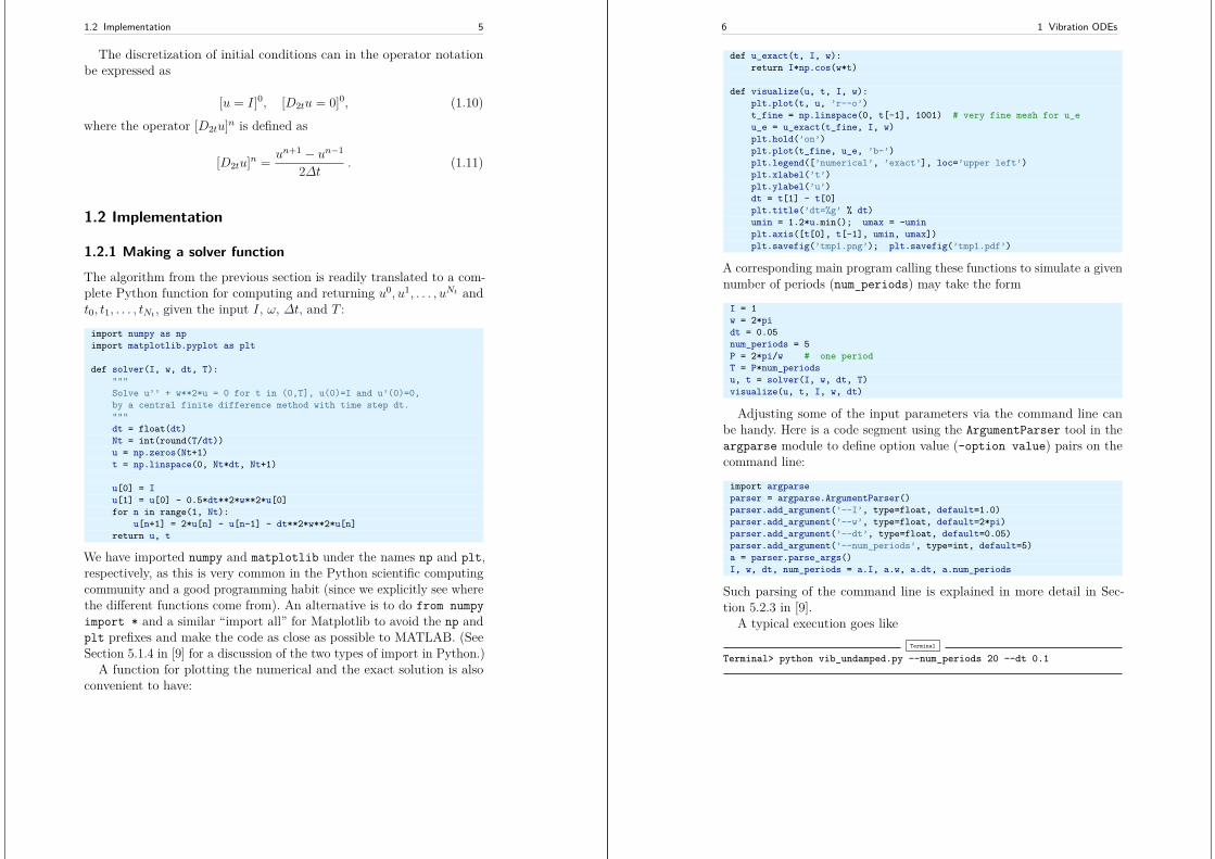
1.2.1 Making a solver functionThe algorithm from the previous section is readily translated to a com-plete Python function for computing and returning u0, u1, . . . , uNt andt0, t1, . . . , tNt , given the input I, ω, ∆t, and T :
import numpy as npimport matplotlib.pyplot as plt
def solver(I, w, dt, T):"""Solve u’’ + w**2*u = 0 for t in (0,T], u(0)=I and u’(0)=0,by a central finite difference method with time step dt."""dt = float(dt)Nt = int(round(T/dt))u = np.zeros(Nt+1)t = np.linspace(0, Nt*dt, Nt+1)
u[0] = Iu[1] = u[0] - 0.5*dt**2*w**2*u[0]for n in range(1, Nt):
u[n+1] = 2*u[n] - u[n-1] - dt**2*w**2*u[n]return u, t
We have imported numpy and matplotlib under the names np and plt,respectively, as this is very common in the Python scientific computingcommunity and a good programming habit (since we explicitly see wherethe different functions come from). An alternative is to do from numpyimport * and a similar “import all” for Matplotlib to avoid the np andplt prefixes and make the code as close as possible to MATLAB. (SeeSection 5.1.4 in [9] for a discussion of the two types of import in Python.)
A function for plotting the numerical and the exact solution is alsoconvenient to have:
6 1 Vibration ODEs
def u_exact(t, I, w):return I*np.cos(w*t)
def visualize(u, t, I, w):plt.plot(t, u, ’r--o’)t_fine = np.linspace(0, t[-1], 1001) # very fine mesh for u_eu_e = u_exact(t_fine, I, w)plt.hold(’on’)plt.plot(t_fine, u_e, ’b-’)plt.legend([’numerical’, ’exact’], loc=’upper left’)plt.xlabel(’t’)plt.ylabel(’u’)dt = t[1] - t[0]plt.title(’dt=%g’ % dt)umin = 1.2*u.min(); umax = -uminplt.axis([t[0], t[-1], umin, umax])plt.savefig(’tmp1.png’); plt.savefig(’tmp1.pdf’)
A corresponding main program calling these functions to simulate a givennumber of periods (num_periods) may take the form
I = 1w = 2*pidt = 0.05num_periods = 5P = 2*pi/w # one periodT = P*num_periodsu, t = solver(I, w, dt, T)visualize(u, t, I, w, dt)
Adjusting some of the input parameters via the command line canbe handy. Here is a code segment using the ArgumentParser tool in theargparse module to define option value (–option value) pairs on thecommand line:
import argparseparser = argparse.ArgumentParser()parser.add_argument(’--I’, type=float, default=1.0)parser.add_argument(’--w’, type=float, default=2*pi)parser.add_argument(’--dt’, type=float, default=0.05)parser.add_argument(’--num_periods’, type=int, default=5)a = parser.parse_args()I, w, dt, num_periods = a.I, a.w, a.dt, a.num_periods
Such parsing of the command line is explained in more detail in Sec-tion 5.2.3 in [9].
A typical execution goes likeTerminal
Terminal> python vib_undamped.py --num_periods 20 --dt 0.1
1.2 Implementation 7
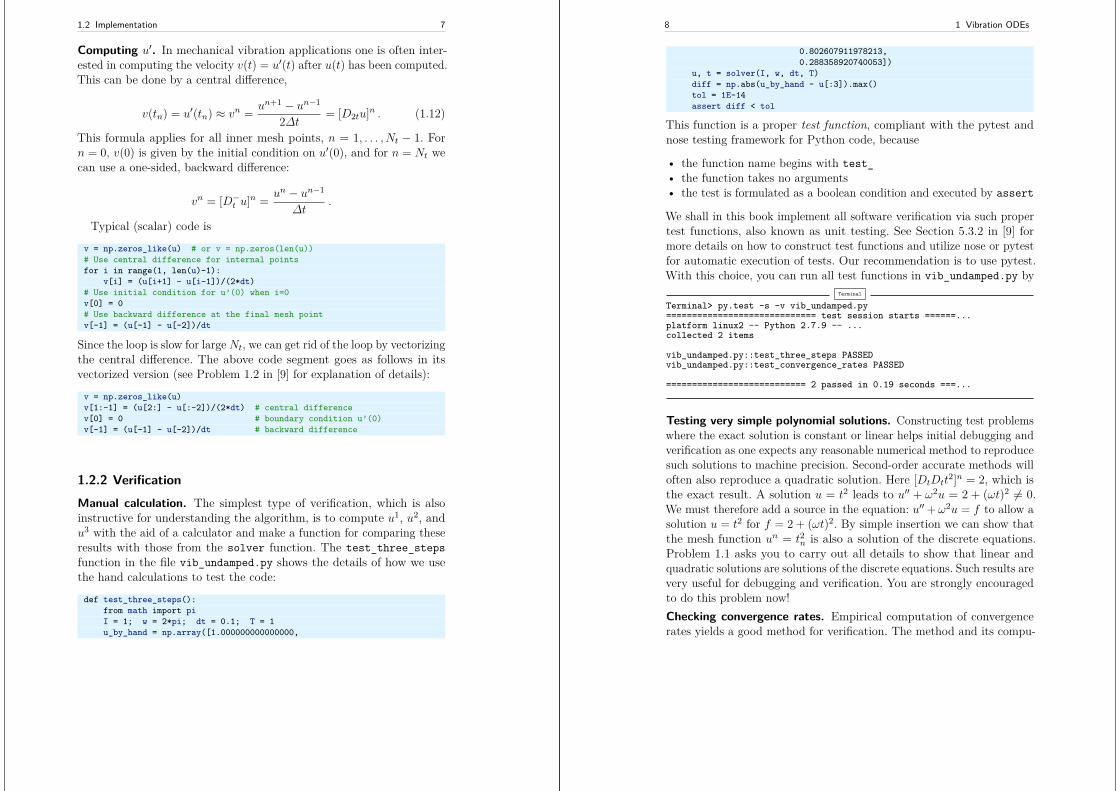
Computing u′. In mechanical vibration applications one is often inter-ested in computing the velocity v(t) = u′(t) after u(t) has been computed.This can be done by a central difference,
v(tn) = u′(tn) ≈ vn = un+1 − un−1
2∆t = [D2tu]n . (1.12)
This formula applies for all inner mesh points, n = 1, . . . , Nt − 1. Forn = 0, v(0) is given by the initial condition on u′(0), and for n = Nt wecan use a one-sided, backward difference:
vn = [D−t u]n = un − un−1
∆t.
Typical (scalar) code is
v = np.zeros_like(u) # or v = np.zeros(len(u))# Use central difference for internal pointsfor i in range(1, len(u)-1):
v[i] = (u[i+1] - u[i-1])/(2*dt)# Use initial condition for u’(0) when i=0v[0] = 0# Use backward difference at the final mesh pointv[-1] = (u[-1] - u[-2])/dt
Since the loop is slow for large Nt, we can get rid of the loop by vectorizingthe central difference. The above code segment goes as follows in itsvectorized version (see Problem 1.2 in [9] for explanation of details):
v = np.zeros_like(u)v[1:-1] = (u[2:] - u[:-2])/(2*dt) # central differencev[0] = 0 # boundary condition u’(0)v[-1] = (u[-1] - u[-2])/dt # backward difference
1.2.2 VerificationManual calculation. The simplest type of verification, which is alsoinstructive for understanding the algorithm, is to compute u1, u2, andu3 with the aid of a calculator and make a function for comparing theseresults with those from the solver function. The test_three_stepsfunction in the file vib_undamped.py shows the details of how we usethe hand calculations to test the code:
def test_three_steps():from math import piI = 1; w = 2*pi; dt = 0.1; T = 1u_by_hand = np.array([1.000000000000000,
8 1 Vibration ODEs
0.802607911978213,0.288358920740053])
u, t = solver(I, w, dt, T)diff = np.abs(u_by_hand - u[:3]).max()tol = 1E-14assert diff < tol
This function is a proper test function, compliant with the pytest andnose testing framework for Python code, because
• the function name begins with test_• the function takes no arguments• the test is formulated as a boolean condition and executed by assert
We shall in this book implement all software verification via such propertest functions, also known as unit testing. See Section 5.3.2 in [9] formore details on how to construct test functions and utilize nose or pytestfor automatic execution of tests. Our recommendation is to use pytest.With this choice, you can run all test functions in vib_undamped.py by
Terminal
Terminal> py.test -s -v vib_undamped.py============================= test session starts ======...platform linux2 -- Python 2.7.9 -- ...collected 2 items
vib_undamped.py::test_three_steps PASSEDvib_undamped.py::test_convergence_rates PASSED
=========================== 2 passed in 0.19 seconds ===...
Testing very simple polynomial solutions. Constructing test problemswhere the exact solution is constant or linear helps initial debugging andverification as one expects any reasonable numerical method to reproducesuch solutions to machine precision. Second-order accurate methods willoften also reproduce a quadratic solution. Here [DtDtt
2]n = 2, which isthe exact result. A solution u = t2 leads to u′′ + ω2u = 2 + (ωt)2 6= 0.We must therefore add a source in the equation: u′′ + ω2u = f to allow asolution u = t2 for f = 2 + (ωt)2. By simple insertion we can show thatthe mesh function un = t2n is also a solution of the discrete equations.Problem 1.1 asks you to carry out all details to show that linear andquadratic solutions are solutions of the discrete equations. Such results arevery useful for debugging and verification. You are strongly encouragedto do this problem now!Checking convergence rates. Empirical computation of convergencerates yields a good method for verification. The method and its compu-
1.2 Implementation 9
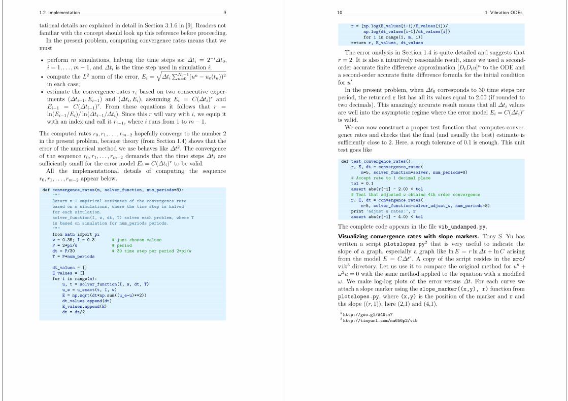
tational details are explained in detail in Section 3.1.6 in [9]. Readers notfamiliar with the concept should look up this reference before proceeding.
In the present problem, computing convergence rates means that wemust
• perform m simulations, halving the time steps as: ∆ti = 2−i∆t0,i = 1, . . . ,m− 1, and ∆ti is the time step used in simulation i;
• compute the L2 norm of the error, Ei =√∆ti
∑Nt−1n=0 (un − ue(tn))2
in each case;• estimate the convergence rates ri based on two consecutive exper-
iments (∆ti−1, Ei−1) and (∆ti, Ei), assuming Ei = C(∆ti)r andEi−1 = C(∆ti−1)r. From these equations it follows that r =ln(Ei−1/Ei)/ ln(∆ti−1/∆ti). Since this r will vary with i, we equip itwith an index and call it ri−1, where i runs from 1 to m− 1.
The computed rates r0, r1, . . . , rm−2 hopefully converge to the number 2in the present problem, because theory (from Section 1.4) shows that theerror of the numerical method we use behaves like ∆t2. The convergenceof the sequence r0, r1, . . . , rm−2 demands that the time steps ∆ti aresufficiently small for the error model Ei = C(∆ti)r to be valid.
All the implementational details of computing the sequencer0, r1, . . . , rm−2 appear below.
def convergence_rates(m, solver_function, num_periods=8):"""Return m-1 empirical estimates of the convergence ratebased on m simulations, where the time step is halvedfor each simulation.solver_function(I, w, dt, T) solves each problem, where Tis based on simulation for num_periods periods."""from math import piw = 0.35; I = 0.3 # just chosen valuesP = 2*pi/w # perioddt = P/30 # 30 time step per period 2*pi/wT = P*num_periods
dt_values = []E_values = []for i in range(m):
u, t = solver_function(I, w, dt, T)u_e = u_exact(t, I, w)E = np.sqrt(dt*np.sum((u_e-u)**2))dt_values.append(dt)E_values.append(E)dt = dt/2
10 1 Vibration ODEs
r = [np.log(E_values[i-1]/E_values[i])/np.log(dt_values[i-1]/dt_values[i])for i in range(1, m, 1)]
return r, E_values, dt_values
The error analysis in Section 1.4 is quite detailed and suggests thatr = 2. It is also a intuitively reasonable result, since we used a second-order accurate finite difference approximation [DtDtu]n to the ODE anda second-order accurate finite difference formula for the initial conditionfor u′.
In the present problem, when ∆t0 corresponds to 30 time steps perperiod, the returned r list has all its values equal to 2.00 (if rounded totwo decimals). This amazingly accurate result means that all ∆ti valuesare well into the asymptotic regime where the error model Ei = C(∆ti)ris valid.
We can now construct a proper test function that computes conver-gence rates and checks that the final (and usually the best) estimate issufficiently close to 2. Here, a rough tolerance of 0.1 is enough. This unittest goes like
def test_convergence_rates():r, E, dt = convergence_rates(
m=5, solver_function=solver, num_periods=8)# Accept rate to 1 decimal placetol = 0.1assert abs(r[-1] - 2.0) < tol# Test that adjusted w obtains 4th order convergencer, E, dt = convergence_rates(
m=5, solver_function=solver_adjust_w, num_periods=8)print ’adjust w rates:’, rassert abs(r[-1] - 4.0) < tol
The complete code appears in the file vib_undamped.py.Visualizing convergence rates with slope markers. Tony S. Yu haswritten a script plotslopes.py2 that is very useful to indicate theslope of a graph, especially a graph like lnE = r ln∆t + lnC arisingfrom the model E = C∆tr. A copy of the script resides in the src/vib3 directory. Let us use it to compare the original method for u′′ +ω2u = 0 with the same method applied to the equation with a modifiedω. We make log-log plots of the error versus ∆t. For each curve weattach a slope marker using the slope_marker((x,y), r) function fromplotslopes.py, where (x,y) is the position of the marker and r andthe slope ((r, 1)), here (2,1) and (4,1).
2 http://goo.gl/A4Utm73 http://tinyurl.com/nu656p2/vib
1.2 Implementation 11
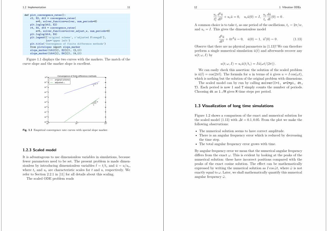
def plot_convergence_rates():r2, E2, dt2 = convergence_rates(
m=5, solver_function=solver, num_periods=8)plt.loglog(dt2, E2)r4, E4, dt4 = convergence_rates(
m=5, solver_function=solver_adjust_w, num_periods=8)plt.loglog(dt4, E4)plt.legend([’original scheme’, r’adjusted $\omega$’],
loc=’upper left’)plt.title(’Convergence of finite difference methods’)from plotslopes import slope_markerslope_marker((dt2[1], E2[1]), (2,1))slope_marker((dt4[1], E4[1]), (4,1))
Figure 1.1 displays the two curves with the markers. The match of thecurve slope and the marker slope is excellent.
10-2 10-1 10010-9
10-8
10-7
10-6
10-5
10-4
10-3
10-2
10-1
100
12
1
4
Convergence of finite difference methods
original schemeadjusted ω
Fig. 1.1 Empirical convergence rate curves with special slope marker.
1.2.3 Scaled model
It is advantageous to use dimensionless variables in simulations, becausefewer parameters need to be set. The present problem is made dimen-sionless by introducing dimensionless variables t = t/tc and u = u/uc,where tc and uc are characteristic scales for t and u, respectively. Werefer to Section 2.2.1 in [11] for all details about this scaling.
The scaled ODE problem reads
12 1 Vibration ODEs
uct2c
d2u
dt2+ ucu = 0, ucu(0) = I,
uctc
du
dt(0) = 0 .
A common choice is to take tc as one period of the oscillations, tc = 2π/w,and uc = I. This gives the dimensionless model
d2u
dt2+ 4π2u = 0, u(0) = 1, u′(0) = 0 . (1.13)
Observe that there are no physical parameters in (1.13)! We can thereforeperform a single numerical simulation u(t) and afterwards recover anyu(t;ω, I) by
u(t;ω, I) = ucu(t/tc) = Iu(ωt/(2π)) .
We can easily check this assertion: the solution of the scaled problemis u(t) = cos(2πt). The formula for u in terms of u gives u = I cos(ωt),which is nothing but the solution of the original problem with dimensions.
The scaled model can by run by calling solver(I=1, w=2*pi, dt,T). Each period is now 1 and T simply counts the number of periods.Choosing dt as 1./M gives M time steps per period.
1.3 Visualization of long time simulations
Figure 1.2 shows a comparison of the exact and numerical solution forthe scaled model (1.13) with ∆t = 0.1, 0.05. From the plot we make thefollowing observations:
• The numerical solution seems to have correct amplitude.• There is an angular frequency error which is reduced by decreasing
the time step.• The total angular frequency error grows with time.
By angular frequency error we mean that the numerical angular frequencydiffers from the exact ω. This is evident by looking at the peaks of thenumerical solution: these have incorrect positions compared with thepeaks of the exact cosine solution. The effect can be mathematicallyexpressed by writing the numerical solution as I cos ωt, where ω is notexactly equal to ω. Later, we shall mathematically quantify this numericalangular frequency ω.
1.3 Visualization of long time simulations 13
0 1 2 3 4 5t
1.0
0.5
0.0
0.5
1.0
u
dt=0.1
numericalexact
0 1 2 3 4 5t
1.0
0.5
0.0
0.5
1.0
u
dt=0.05
numericalexact
Fig. 1.2 Effect of halving the time step.
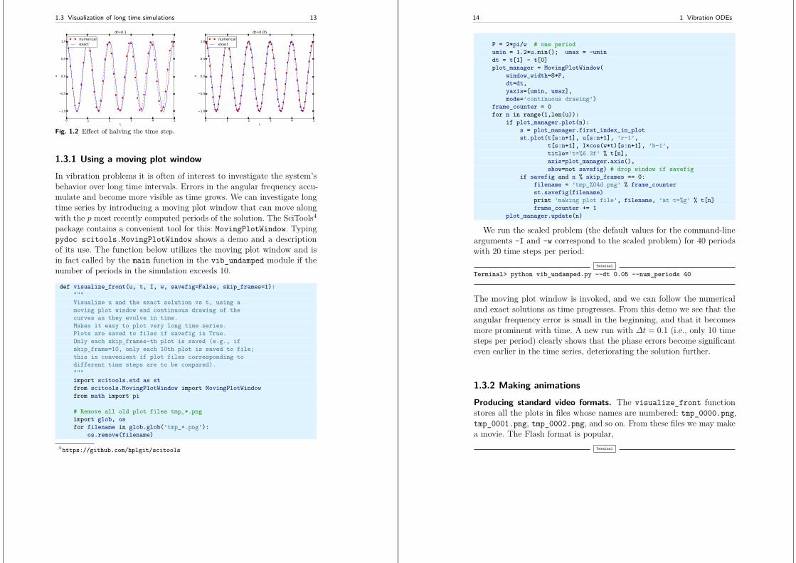
1.3.1 Using a moving plot windowIn vibration problems it is often of interest to investigate the system’sbehavior over long time intervals. Errors in the angular frequency accu-mulate and become more visible as time grows. We can investigate longtime series by introducing a moving plot window that can move alongwith the p most recently computed periods of the solution. The SciTools4
package contains a convenient tool for this: MovingPlotWindow. Typingpydoc scitools.MovingPlotWindow shows a demo and a descriptionof its use. The function below utilizes the moving plot window and isin fact called by the main function in the vib_undamped module if thenumber of periods in the simulation exceeds 10.
def visualize_front(u, t, I, w, savefig=False, skip_frames=1):"""Visualize u and the exact solution vs t, using amoving plot window and continuous drawing of thecurves as they evolve in time.Makes it easy to plot very long time series.Plots are saved to files if savefig is True.Only each skip_frames-th plot is saved (e.g., ifskip_frame=10, only each 10th plot is saved to file;this is convenient if plot files corresponding todifferent time steps are to be compared)."""import scitools.std as stfrom scitools.MovingPlotWindow import MovingPlotWindowfrom math import pi
# Remove all old plot files tmp_*.pngimport glob, osfor filename in glob.glob(’tmp_*.png’):
os.remove(filename)
4 https://github.com/hplgit/scitools
14 1 Vibration ODEs
P = 2*pi/w # one periodumin = 1.2*u.min(); umax = -umindt = t[1] - t[0]plot_manager = MovingPlotWindow(
window_width=8*P,dt=dt,yaxis=[umin, umax],mode=’continuous drawing’)
frame_counter = 0for n in range(1,len(u)):
if plot_manager.plot(n):s = plot_manager.first_index_in_plotst.plot(t[s:n+1], u[s:n+1], ’r-1’,
t[s:n+1], I*cos(w*t)[s:n+1], ’b-1’,title=’t=%6.3f’ % t[n],axis=plot_manager.axis(),show=not savefig) # drop window if savefig
if savefig and n % skip_frames == 0:filename = ’tmp_%04d.png’ % frame_counterst.savefig(filename)print ’making plot file’, filename, ’at t=%g’ % t[n]frame_counter += 1
plot_manager.update(n)
We run the scaled problem (the default values for the command-linearguments –I and –w correspond to the scaled problem) for 40 periodswith 20 time steps per period:
Terminal
Terminal> python vib_undamped.py --dt 0.05 --num_periods 40
The moving plot window is invoked, and we can follow the numericaland exact solutions as time progresses. From this demo we see that theangular frequency error is small in the beginning, and that it becomesmore prominent with time. A new run with ∆t = 0.1 (i.e., only 10 timesteps per period) clearly shows that the phase errors become significanteven earlier in the time series, deteriorating the solution further.
1.3.2 Making animations
Producing standard video formats. The visualize_front functionstores all the plots in files whose names are numbered: tmp_0000.png,tmp_0001.png, tmp_0002.png, and so on. From these files we may makea movie. The Flash format is popular,
Terminal

1.3 Visualization of long time simulations 15
Terminal> ffmpeg -r 25 -i tmp_%04d.png -c:v flv movie.flv
The ffmpeg program can be replaced by the avconv program in theabove command if desired (but at the time of this writing it seems tobe more momentum in the ffmpeg project). The -r option should comefirst and describes the number of frames per second in the movie (evenif we would like to have slow movies, keep this number as large as 25,otherwise files are skipped from the movie). The -i option describes thename of the plot files. Other formats can be generated by changing thevideo codec and equipping the video file with the right extension:
Format Codec and filenameFlash -c:v flv movie.flvMP4 -c:v libx264 movie.mp4WebM -c:v libvpx movie.webmOgg -c:v libtheora movie.ogg
The video file can be played by some video player like vlc, mplayer,gxine, or totem, e.g.,
Terminal
Terminal> vlc movie.webm
A web page can also be used to play the movie. Today’s standard is touse the HTML5 video tag:
<video autoplay loop controlswidth=’640’ height=’365’ preload=’none’>
<source src=’movie.webm’ type=’video/webm; codecs="vp8, vorbis"’></video>
Modern browsers do not support all of the video formats. MP4 is neededto successfully play the videos on Apple devices that use the Safaribrowser. WebM is the preferred format for Chrome, Opera, Firefox, andInternet Explorer v9+. Flash was a popular format, but older browsersthat required Flash can play MP4. All browsers that work with Oggcan also work with WebM. This means that to have a video work in allbrowsers, the video should be available in the MP4 and WebM formats.The proper HTML code reads
<video autoplay loop controlswidth=’640’ height=’365’ preload=’none’>
<source src=’movie.mp4’ type=’video/mp4;codecs="avc1.42E01E, mp4a.40.2"’>
<source src=’movie.webm’ type=’video/webm;
16 1 Vibration ODEs
codecs="vp8, vorbis"’></video>
The MP4 format should appear first to ensure that Apple devices willload the video correctly.
Caution: number the plot files correctly
To ensure that the individual plot frames are shown in correct order,it is important to number the files with zero-padded numbers (0000,0001, 0002, etc.). The printf format %04d specifies an integer in afield of width 4, padded with zeros from the left. A simple Unixwildcard file specification like tmp_*.png will then list the framesin the right order. If the numbers in the filenames were not zero-padded, the frame tmp_11.png would appear before tmp_2.png inthe movie.
Playing PNG files in a web browser. The scitools movie commandcan create a movie player for a set of PNG files such that a web browsercan be used to watch the movie. This interface has the advantage thatthe speed of the movie can easily be controlled, a feature that scientistsoften appreciate. The command for creating an HTML with a player fora set of PNG files tmp_*.png goes like
Terminal
Terminal> scitools movie output_file=vib.html fps=4 tmp_*.png
The fps argument controls the speed of the movie (“frames per second”).To watch the movie, load the video file vib.html into some browser,
e.g.,Terminal
Terminal> google-chrome vib.html # invoke web page
Clicking on Start movie to see the result. Moving this movie to someother place requires moving vib.html and all the PNG files tmp_*.png:
Terminal
Terminal> mkdir vib_dt0.1Terminal> mv tmp_*.png vib_dt0.1Terminal> mv vib.html vib_dt0.1/index.html
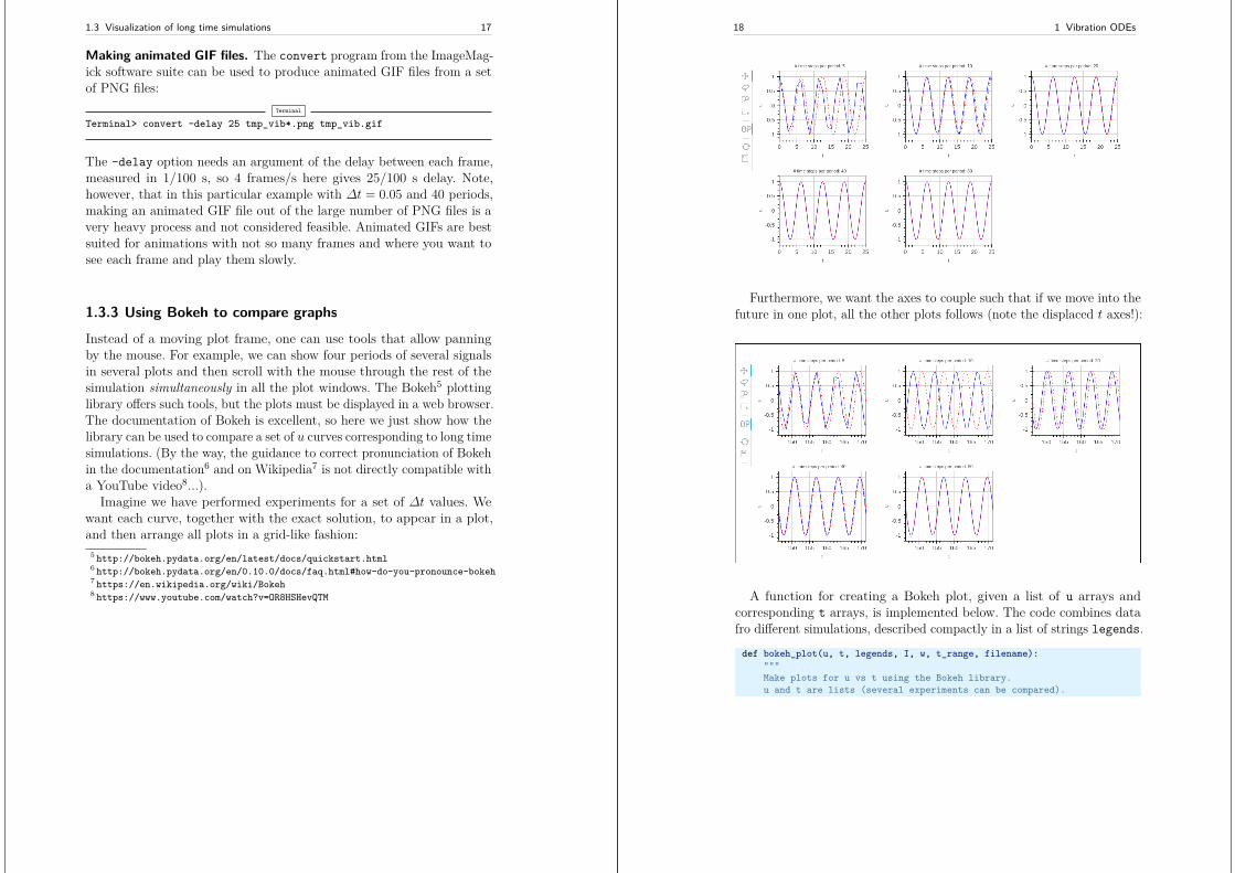
1.3 Visualization of long time simulations 17
Making animated GIF files. The convert program from the ImageMag-ick software suite can be used to produce animated GIF files from a setof PNG files:
Terminal
Terminal> convert -delay 25 tmp_vib*.png tmp_vib.gif
The -delay option needs an argument of the delay between each frame,measured in 1/100 s, so 4 frames/s here gives 25/100 s delay. Note,however, that in this particular example with ∆t = 0.05 and 40 periods,making an animated GIF file out of the large number of PNG files is avery heavy process and not considered feasible. Animated GIFs are bestsuited for animations with not so many frames and where you want tosee each frame and play them slowly.
1.3.3 Using Bokeh to compare graphs
Instead of a moving plot frame, one can use tools that allow panningby the mouse. For example, we can show four periods of several signalsin several plots and then scroll with the mouse through the rest of thesimulation simultaneously in all the plot windows. The Bokeh5 plottinglibrary offers such tools, but the plots must be displayed in a web browser.The documentation of Bokeh is excellent, so here we just show how thelibrary can be used to compare a set of u curves corresponding to long timesimulations. (By the way, the guidance to correct pronunciation of Bokehin the documentation6 and on Wikipedia7 is not directly compatible witha YouTube video8...).
Imagine we have performed experiments for a set of ∆t values. Wewant each curve, together with the exact solution, to appear in a plot,and then arrange all plots in a grid-like fashion:
5 http://bokeh.pydata.org/en/latest/docs/quickstart.html6 http://bokeh.pydata.org/en/0.10.0/docs/faq.html#how-do-you-pronounce-bokeh7 https://en.wikipedia.org/wiki/Bokeh8 https://www.youtube.com/watch?v=OR8HSHevQTM
18 1 Vibration ODEs
Furthermore, we want the axes to couple such that if we move into thefuture in one plot, all the other plots follows (note the displaced t axes!):
A function for creating a Bokeh plot, given a list of u arrays andcorresponding t arrays, is implemented below. The code combines datafro different simulations, described compactly in a list of strings legends.
def bokeh_plot(u, t, legends, I, w, t_range, filename):"""Make plots for u vs t using the Bokeh library.u and t are lists (several experiments can be compared).
1.3 Visualization of long time simulations 19
legens contain legend strings for the various u,t pairs."""if not isinstance(u, (list,tuple)):
u = [u] # wrap in listif not isinstance(t, (list,tuple)):
t = [t] # wrap in listif not isinstance(legends, (list,tuple)):
legends = [legends] # wrap in list
import bokeh.plotting as pltplt.output_file(filename, mode=’cdn’, title=’Comparison’)# Assume that all t arrays have the same ranget_fine = np.linspace(0, t[0][-1], 1001) # fine mesh for u_etools = ’pan,wheel_zoom,box_zoom,reset,’\
’save,box_select,lasso_select’u_range = [-1.2*I, 1.2*I]font_size = ’8pt’p = [] # list of plot objects# Make the first figurep_ = plt.figure(
width=300, plot_height=250, title=legends[0],x_axis_label=’t’, y_axis_label=’u’,x_range=t_range, y_range=u_range, tools=tools,title_text_font_size=font_size)
p_.xaxis.axis_label_text_font_size=font_sizep_.yaxis.axis_label_text_font_size=font_sizep_.line(t[0], u[0], line_color=’blue’)# Add exact solutionu_e = u_exact(t_fine, I, w)p_.line(t_fine, u_e, line_color=’red’, line_dash=’4 4’)p.append(p_)# Make the rest of the figures and attach their axes to# the first figure’s axesfor i in range(1, len(t)):
p_ = plt.figure(width=300, plot_height=250, title=legends[i],x_axis_label=’t’, y_axis_label=’u’,x_range=p[0].x_range, y_range=p[0].y_range, tools=tools,title_text_font_size=font_size)
p_.xaxis.axis_label_text_font_size = font_sizep_.yaxis.axis_label_text_font_size = font_sizep_.line(t[i], u[i], line_color=’blue’)p_.line(t_fine, u_e, line_color=’red’, line_dash=’4 4’)p.append(p_)
# Arrange all plots in a grid with 3 plots per rowgrid = [[]]for i, p_ in enumerate(p):
grid[-1].append(p_)if (i+1) % 3 == 0:
# New rowgrid.append([])
plot = plt.gridplot(grid, toolbar_location=’left’)plt.save(plot)
20 1 Vibration ODEs
plt.show(plot)
A particular example using the bokeh_plot function appears below.
def demo_bokeh():"""Solve a scaled ODE u’’ + u = 0."""from math import piw = 1.0 # Scaled problem (frequency)P = 2*np.pi/w # Periodnum_steps_per_period = [5, 10, 20, 40, 80]T = 40*P # Simulation time: 40 periodsu = [] # List of numerical solutionst = [] # List of corresponding mesheslegends = []for n in num_steps_per_period:
dt = P/nu_, t_ = solver(I=1, w=w, dt=dt, T=T)u.append(u_)t.append(t_)legends.append(’# time steps per period: %d’ % n)
bokeh_plot(u, t, legends, I=1, w=w, t_range=[0, 4*P],filename=’tmp.html’)
1.3.4 Using a line-by-line ascii plotter
Plotting functions vertically, line by line, in the terminal window us-ing ascii characters only is a simple, fast, and convenient visualizationtechnique for long time series. Note that the time axis then is positivedownwards on the screen, so we can let the solution be visualized “for-ever”. The tool scitools.avplotter.Plotter makes it easy to createsuch plots:
def visualize_front_ascii(u, t, I, w, fps=10):"""Plot u and the exact solution vs t line by line in aterminal window (only using ascii characters).Makes it easy to plot very long time series."""from scitools.avplotter import Plotterimport timefrom math import piP = 2*pi/wumin = 1.2*u.min(); umax = -umin
p = Plotter(ymin=umin, ymax=umax, width=60, symbols=’+o’)for n in range(len(u)):
print p.plot(t[n], u[n], I*cos(w*t[n])), \’%.1f’ % (t[n]/P)
time.sleep(1/float(fps))
1.3 Visualization of long time simulations 21
The call p.plot returns a line of text, with the t axis marked and asymbol + for the first function (u) and o for the second function (theexact solution). Here we append to this text a time counter reflecting howmany periods the current time point corresponds to. A typical output(ω = 2π, ∆t = 0.05) looks like this:
| o+ 14.0| + o 14.0| + o 14.1| + o 14.1| + o 14.2
+| o 14.2+ | 14.2
+ o | 14.3+ o | 14.4
+ o | 14.4+o | 14.5o + | 14.5o + | 14.6
o + | 14.6o + | 14.7
o | + 14.7| + 14.8| o + 14.8| o + 14.9| o + 14.9| o+ 15.0
1.3.5 Empirical analysis of the solutionFor oscillating functions like those in Figure 1.2 we may compute theamplitude and frequency (or period) empirically. That is, we run throughthe discrete solution points (tn, un) and find all maxima and minimapoints. The distance between two consecutive maxima (or minima) pointscan be used as estimate of the local period, while half the differencebetween the u value at a maximum and a nearby minimum gives anestimate of the local amplitude.
The local maxima are the points where
un−1 < un > un+1, n = 1, . . . , Nt − 1, (1.14)
and the local minima are recognized by
un−1 > un < un+1, n = 1, . . . , Nt − 1 . (1.15)
In computer code this becomes
22 1 Vibration ODEs
def minmax(t, u):minima = []; maxima = []for n in range(1, len(u)-1, 1):
if u[n-1] > u[n] < u[n+1]:minima.append((t[n], u[n]))
if u[n-1] < u[n] > u[n+1]:maxima.append((t[n], u[n]))
return minima, maxima
Note that the two returned objects are lists of tuples.Let (ti, ei), i = 0, . . . ,M − 1, be the sequence of all the M maxima
points, where ti is the time value and ei the corresponding u value. Thelocal period can be defined as pi = ti+1 − ti. With Python syntax thisreads
def periods(maxima):p = [extrema[n][0] - maxima[n-1][0]
for n in range(1, len(maxima))]return np.array(p)
The list p created by a list comprehension is converted to an arraysince we probably want to compute with it, e.g., find the correspondingfrequencies 2*pi/p.
Having the minima and the maxima, the local amplitude can becalculated as the difference between two neighboring minimum andmaximum points:
def amplitudes(minima, maxima):a = [(abs(maxima[n][1] - minima[n][1]))/2.0
for n in range(min(len(minima),len(maxima)))]return np.array(a)
The code segments are found in the file vib_empirical_analysis.py.Since a[i] and p[i] correspond to the i-th amplitude estimate and
the i-th period estimate, respectively, it is most convenient to visualizethe a and p values with the index i on the horizontal axis. (There is nounique time point associated with either of these estimate since valuesat two different time points were used in the computations.)
In the analysis of very long time series, it is advantageous to computeand plot p and a instead of u to get an impression of the developmentof the oscillations. Let us do this for the scaled problem and ∆t =0.1, 0.05, 0.01. A ready-made function
plot_empirical_freq_and_amplitude(u, t, I, w)
computes the empirical amplitudes and periods, and creates a plot wherethe amplitudes and angular frequencies are visualized together with the
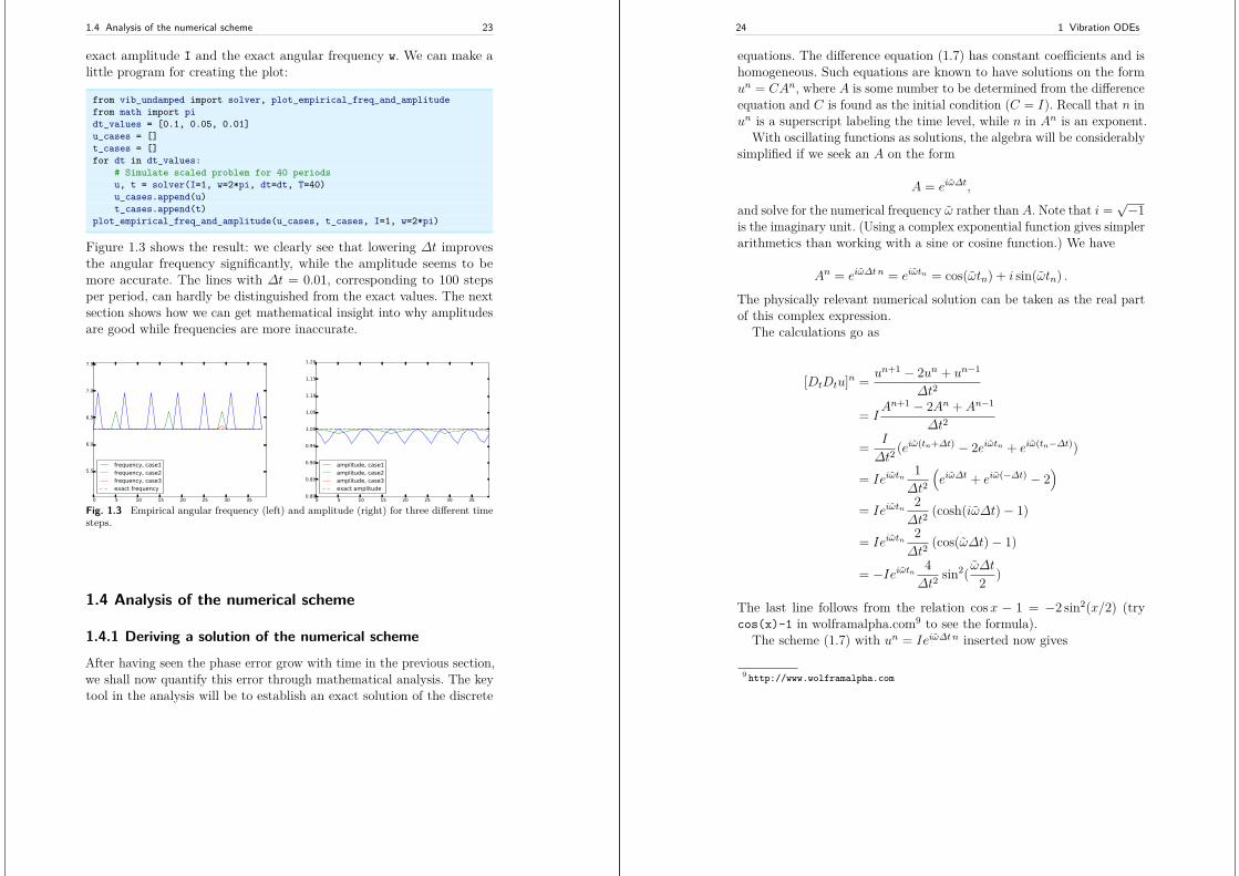
1.4 Analysis of the numerical scheme 23
exact amplitude I and the exact angular frequency w. We can make alittle program for creating the plot:
from vib_undamped import solver, plot_empirical_freq_and_amplitudefrom math import pidt_values = [0.1, 0.05, 0.01]u_cases = []t_cases = []for dt in dt_values:
# Simulate scaled problem for 40 periodsu, t = solver(I=1, w=2*pi, dt=dt, T=40)u_cases.append(u)t_cases.append(t)
plot_empirical_freq_and_amplitude(u_cases, t_cases, I=1, w=2*pi)
Figure 1.3 shows the result: we clearly see that lowering ∆t improvesthe angular frequency significantly, while the amplitude seems to bemore accurate. The lines with ∆t = 0.01, corresponding to 100 stepsper period, can hardly be distinguished from the exact values. The nextsection shows how we can get mathematical insight into why amplitudesare good while frequencies are more inaccurate.
0 5 10 15 20 25 30 35
5.5
6.0
6.5
7.0
7.5
frequency, case1frequency, case2frequency, case3exact frequency
0 5 10 15 20 25 30 350.80
0.85
0.90
0.95
1.00
1.05
1.10
1.15
1.20
amplitude, case1amplitude, case2amplitude, case3exact amplitude
Fig. 1.3 Empirical angular frequency (left) and amplitude (right) for three different timesteps.
1.4 Analysis of the numerical scheme
1.4.1 Deriving a solution of the numerical scheme
After having seen the phase error grow with time in the previous section,we shall now quantify this error through mathematical analysis. The keytool in the analysis will be to establish an exact solution of the discrete
24 1 Vibration ODEs
equations. The difference equation (1.7) has constant coefficients and ishomogeneous. Such equations are known to have solutions on the formun = CAn, where A is some number to be determined from the differenceequation and C is found as the initial condition (C = I). Recall that n inun is a superscript labeling the time level, while n in An is an exponent.
With oscillating functions as solutions, the algebra will be considerablysimplified if we seek an A on the form
A = eiω∆t,
and solve for the numerical frequency ω rather than A. Note that i =√−1
is the imaginary unit. (Using a complex exponential function gives simplerarithmetics than working with a sine or cosine function.) We have
An = eiω∆t n = eiωtn = cos(ωtn) + i sin(ωtn) .
The physically relevant numerical solution can be taken as the real partof this complex expression.
The calculations go as
[DtDtu]n = un+1 − 2un + un−1
∆t2
= IAn+1 − 2An + An−1
∆t2
= I
∆t2(eiω(tn+∆t) − 2eiωtn + eiω(tn−∆t))
= Ieiωtn1∆t2
(eiω∆t + eiω(−∆t) − 2
)
= Ieiωtn2∆t2
(cosh(iω∆t)− 1)
= Ieiωtn2∆t2
(cos(ω∆t)− 1)
= −Ieiωtn 4∆t2
sin2( ω∆t2 )
The last line follows from the relation cosx − 1 = −2 sin2(x/2) (trycos(x)-1 in wolframalpha.com9 to see the formula).
The scheme (1.7) with un = Ieiω∆t n inserted now gives
9 http://www.wolframalpha.com
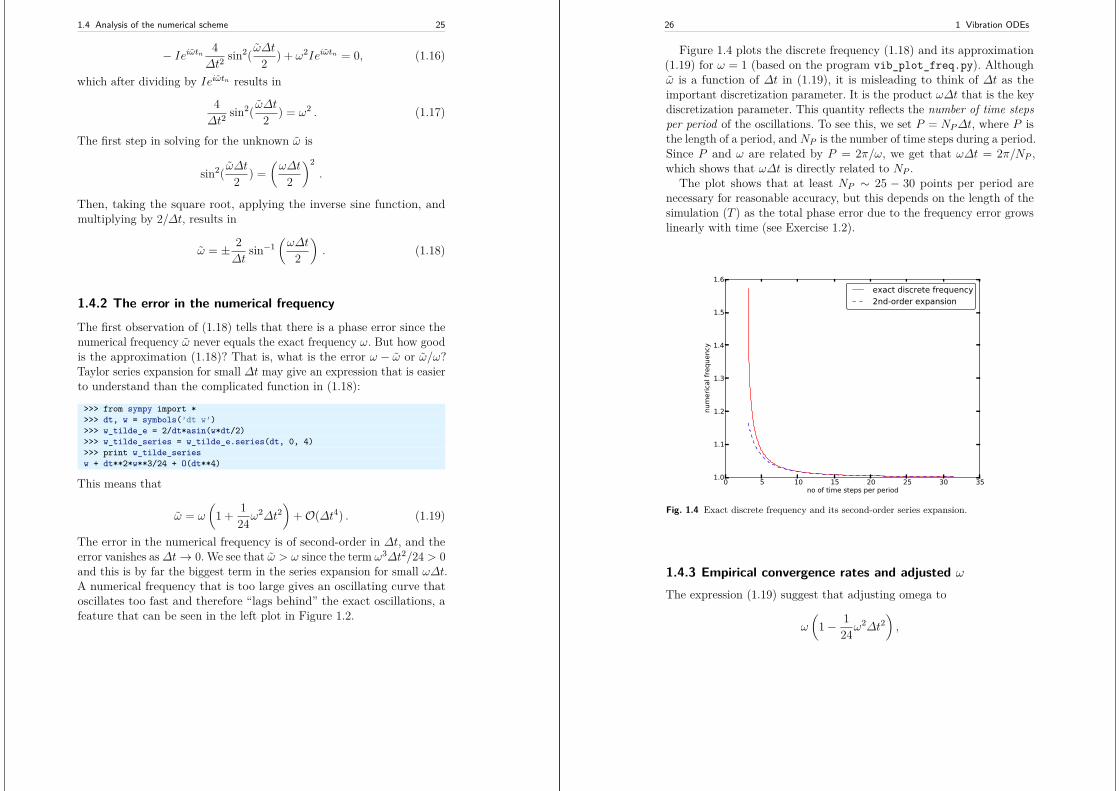
1.4 Analysis of the numerical scheme 25
− Ieiωtn 4∆t2
sin2( ω∆t2 ) + ω2Ieiωtn = 0, (1.16)
which after dividing by Ieiωtn results in
4∆t2
sin2( ω∆t2 ) = ω2 . (1.17)
The first step in solving for the unknown ω is
sin2( ω∆t2 ) =(ω∆t
2
)2.
Then, taking the square root, applying the inverse sine function, andmultiplying by 2/∆t, results in
ω = ± 2∆t
sin−1(ω∆t
2
). (1.18)
1.4.2 The error in the numerical frequency
The first observation of (1.18) tells that there is a phase error since thenumerical frequency ω never equals the exact frequency ω. But how goodis the approximation (1.18)? That is, what is the error ω − ω or ω/ω?Taylor series expansion for small ∆t may give an expression that is easierto understand than the complicated function in (1.18):
>>> from sympy import *>>> dt, w = symbols(’dt w’)>>> w_tilde_e = 2/dt*asin(w*dt/2)>>> w_tilde_series = w_tilde_e.series(dt, 0, 4)>>> print w_tilde_seriesw + dt**2*w**3/24 + O(dt**4)
This means that
ω = ω
(1 + 1
24ω2∆t2
)+O(∆t4) . (1.19)
The error in the numerical frequency is of second-order in ∆t, and theerror vanishes as∆t→ 0. We see that ω > ω since the term ω3∆t2/24 > 0and this is by far the biggest term in the series expansion for small ω∆t.A numerical frequency that is too large gives an oscillating curve thatoscillates too fast and therefore “lags behind” the exact oscillations, afeature that can be seen in the left plot in Figure 1.2.
26 1 Vibration ODEs
Figure 1.4 plots the discrete frequency (1.18) and its approximation(1.19) for ω = 1 (based on the program vib_plot_freq.py). Althoughω is a function of ∆t in (1.19), it is misleading to think of ∆t as theimportant discretization parameter. It is the product ω∆t that is the keydiscretization parameter. This quantity reflects the number of time stepsper period of the oscillations. To see this, we set P = NP∆t, where P isthe length of a period, and NP is the number of time steps during a period.Since P and ω are related by P = 2π/ω, we get that ω∆t = 2π/NP ,which shows that ω∆t is directly related to NP .
The plot shows that at least NP ∼ 25 − 30 points per period arenecessary for reasonable accuracy, but this depends on the length of thesimulation (T ) as the total phase error due to the frequency error growslinearly with time (see Exercise 1.2).
0 5 10 15 20 25 30 35no of time steps per period
1.0
1.1
1.2
1.3
1.4
1.5
1.6
num
eric
al fr
eque
ncy
exact discrete frequency2nd-order expansion
Fig. 1.4 Exact discrete frequency and its second-order series expansion.
1.4.3 Empirical convergence rates and adjusted ωThe expression (1.19) suggest that adjusting omega to
ω
(1− 1
24ω2∆t2
),
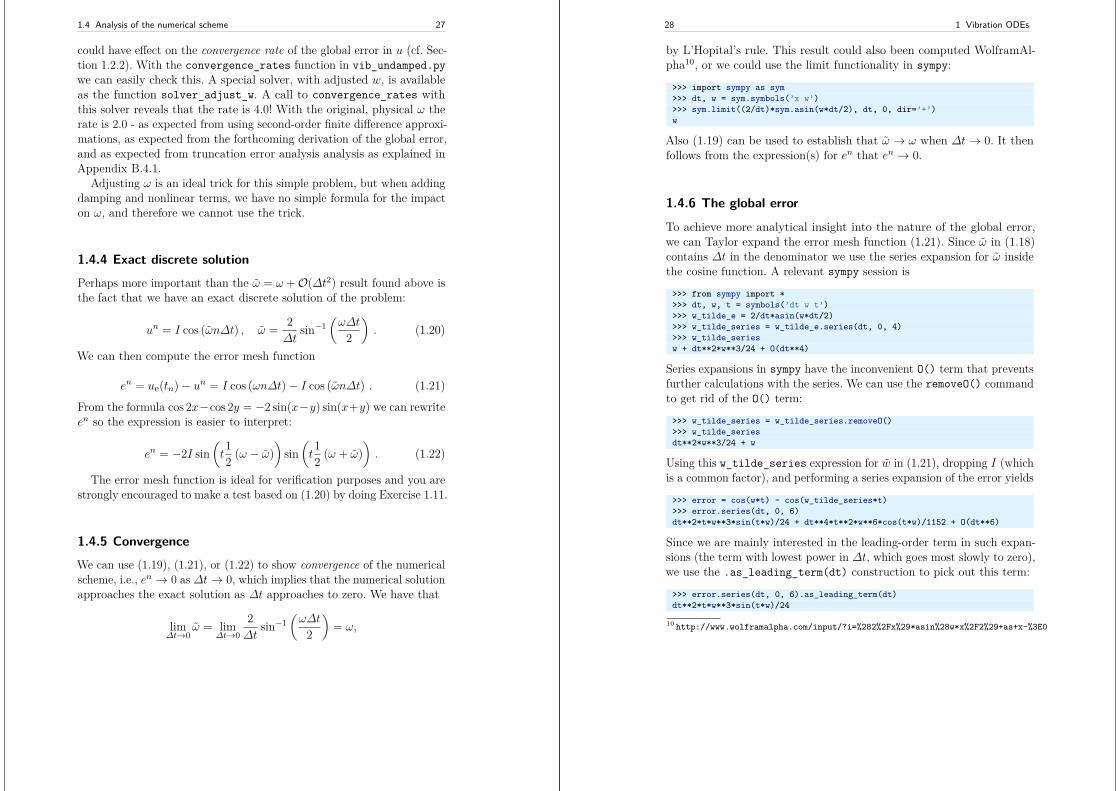
1.4 Analysis of the numerical scheme 27
could have effect on the convergence rate of the global error in u (cf. Sec-tion 1.2.2). With the convergence_rates function in vib_undamped.pywe can easily check this. A special solver, with adjusted w, is availableas the function solver_adjust_w. A call to convergence_rates withthis solver reveals that the rate is 4.0! With the original, physical ω therate is 2.0 - as expected from using second-order finite difference approxi-mations, as expected from the forthcoming derivation of the global error,and as expected from truncation error analysis analysis as explained inAppendix B.4.1.
Adjusting ω is an ideal trick for this simple problem, but when addingdamping and nonlinear terms, we have no simple formula for the impacton ω, and therefore we cannot use the trick.
1.4.4 Exact discrete solutionPerhaps more important than the ω = ω +O(∆t2) result found above isthe fact that we have an exact discrete solution of the problem:
un = I cos (ωn∆t) , ω = 2∆t
sin−1(ω∆t
2
). (1.20)
We can then compute the error mesh function
en = ue(tn)− un = I cos (ωn∆t)− I cos (ωn∆t) . (1.21)
From the formula cos 2x−cos 2y = −2 sin(x−y) sin(x+y) we can rewriteen so the expression is easier to interpret:
en = −2I sin(t12 (ω − ω)
)sin(t12 (ω + ω)
). (1.22)
The error mesh function is ideal for verification purposes and you arestrongly encouraged to make a test based on (1.20) by doing Exercise 1.11.
1.4.5 ConvergenceWe can use (1.19), (1.21), or (1.22) to show convergence of the numericalscheme, i.e., en → 0 as ∆t→ 0, which implies that the numerical solutionapproaches the exact solution as ∆t approaches to zero. We have that
lim∆t→0
ω = lim∆t→0
2∆t
sin−1(ω∆t
2
)= ω,
28 1 Vibration ODEs
by L’Hopital’s rule. This result could also been computed WolframAl-pha10, or we could use the limit functionality in sympy:
>>> import sympy as sym>>> dt, w = sym.symbols(’x w’)>>> sym.limit((2/dt)*sym.asin(w*dt/2), dt, 0, dir=’+’)w
Also (1.19) can be used to establish that ω → ω when ∆t→ 0. It thenfollows from the expression(s) for en that en → 0.
1.4.6 The global error
To achieve more analytical insight into the nature of the global error,we can Taylor expand the error mesh function (1.21). Since ω in (1.18)contains ∆t in the denominator we use the series expansion for ω insidethe cosine function. A relevant sympy session is
>>> from sympy import *>>> dt, w, t = symbols(’dt w t’)>>> w_tilde_e = 2/dt*asin(w*dt/2)>>> w_tilde_series = w_tilde_e.series(dt, 0, 4)>>> w_tilde_seriesw + dt**2*w**3/24 + O(dt**4)
Series expansions in sympy have the inconvenient O() term that preventsfurther calculations with the series. We can use the removeO() commandto get rid of the O() term:
>>> w_tilde_series = w_tilde_series.removeO()>>> w_tilde_seriesdt**2*w**3/24 + w
Using this w_tilde_series expression for w in (1.21), dropping I (whichis a common factor), and performing a series expansion of the error yields
>>> error = cos(w*t) - cos(w_tilde_series*t)>>> error.series(dt, 0, 6)dt**2*t*w**3*sin(t*w)/24 + dt**4*t**2*w**6*cos(t*w)/1152 + O(dt**6)
Since we are mainly interested in the leading-order term in such expan-sions (the term with lowest power in ∆t, which goes most slowly to zero),we use the .as_leading_term(dt) construction to pick out this term:
>>> error.series(dt, 0, 6).as_leading_term(dt)dt**2*t*w**3*sin(t*w)/24
10 http://www.wolframalpha.com/input/?i=%282%2Fx%29*asin%28w*x%2F2%29+as+x-%3E0
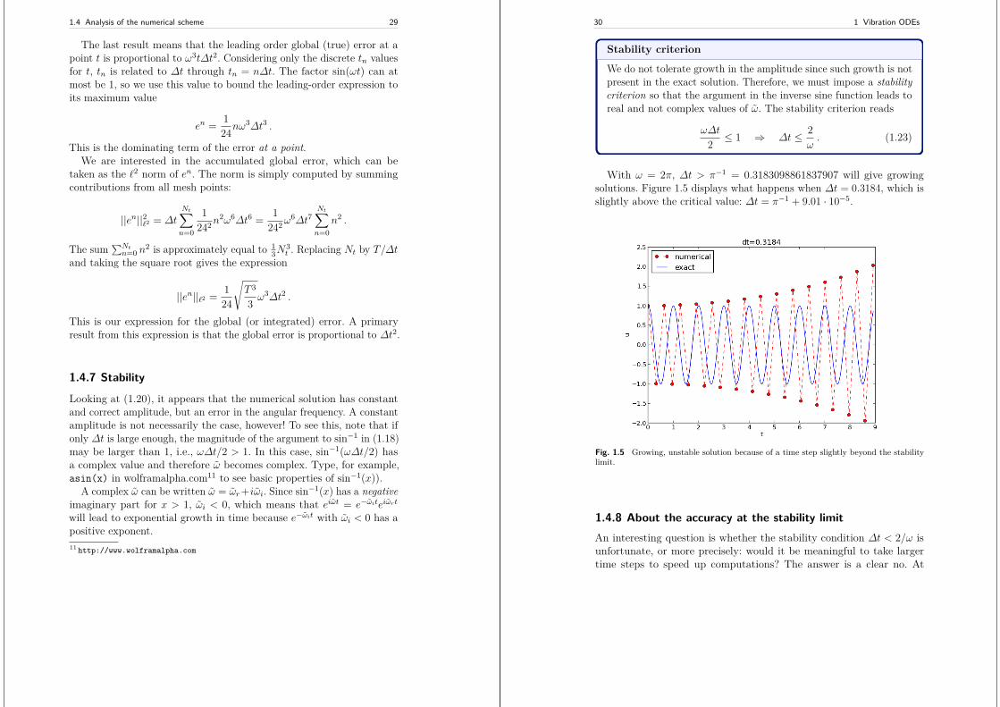
1.4 Analysis of the numerical scheme 29
The last result means that the leading order global (true) error at apoint t is proportional to ω3t∆t2. Considering only the discrete tn valuesfor t, tn is related to ∆t through tn = n∆t. The factor sin(ωt) can atmost be 1, so we use this value to bound the leading-order expression toits maximum value
en = 124nω
3∆t3 .
This is the dominating term of the error at a point.We are interested in the accumulated global error, which can be
taken as the `2 norm of en. The norm is simply computed by summingcontributions from all mesh points:
||en||2`2 = ∆tNt∑
n=0
1242n
2ω6∆t6 = 1242ω
6∆t7Nt∑
n=0n2 .
The sum∑Ntn=0 n
2 is approximately equal to 13N
3t . Replacing Nt by T/∆t
and taking the square root gives the expression
||en||`2 = 124
√T 3
3 ω3∆t2 .
This is our expression for the global (or integrated) error. A primaryresult from this expression is that the global error is proportional to ∆t2.
1.4.7 Stability
Looking at (1.20), it appears that the numerical solution has constantand correct amplitude, but an error in the angular frequency. A constantamplitude is not necessarily the case, however! To see this, note that ifonly ∆t is large enough, the magnitude of the argument to sin−1 in (1.18)may be larger than 1, i.e., ω∆t/2 > 1. In this case, sin−1(ω∆t/2) hasa complex value and therefore ω becomes complex. Type, for example,asin(x) in wolframalpha.com11 to see basic properties of sin−1(x)).
A complex ω can be written ω = ωr+iωi. Since sin−1(x) has a negativeimaginary part for x > 1, ωi < 0, which means that eiωt = e−ωiteiωrt
will lead to exponential growth in time because e−ωit with ωi < 0 has apositive exponent.11 http://www.wolframalpha.com
30 1 Vibration ODEs
Stability criterion
We do not tolerate growth in the amplitude since such growth is notpresent in the exact solution. Therefore, we must impose a stabilitycriterion so that the argument in the inverse sine function leads toreal and not complex values of ω. The stability criterion reads
ω∆t
2 ≤ 1 ⇒ ∆t ≤ 2ω. (1.23)
With ω = 2π, ∆t > π−1 = 0.3183098861837907 will give growingsolutions. Figure 1.5 displays what happens when ∆t = 0.3184, which isslightly above the critical value: ∆t = π−1 + 9.01 · 10−5.
Fig. 1.5 Growing, unstable solution because of a time step slightly beyond the stabilitylimit.
1.4.8 About the accuracy at the stability limitAn interesting question is whether the stability condition ∆t < 2/ω isunfortunate, or more precisely: would it be meaningful to take largertime steps to speed up computations? The answer is a clear no. At
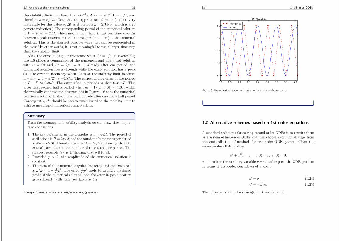
1.4 Analysis of the numerical scheme 31
the stability limit, we have that sin−1 ω∆t/2 = sin−1 1 = π/2, andtherefore ω = π/∆t. (Note that the approximate formula (1.19) is veryinaccurate for this value of ∆t as it predicts ω = 2.34/pi, which is a 25percent reduction.) The corresponding period of the numerical solutionis P = 2π/ω = 2∆t, which means that there is just one time step ∆tbetween a peak (maximum) and a through12 (minimum) in the numericalsolution. This is the shortest possible wave that can be represented inthe mesh! In other words, it is not meaningful to use a larger time stepthan the stability limit.
Also, the error in angular frequency when ∆t = 2/ω is severe: Fig-ure 1.6 shows a comparison of the numerical and analytical solutionwith ω = 2π and ∆t = 2/ω = π−1. Already after one period, thenumerical solution has a through while the exact solution has a peak(!). The error in frequency when ∆t is at the stability limit becomesω − ω = ω(1 − π/2) ≈ −0.57ω. The corresponding error in the periodis P − P ≈ 0.36P . The error after m periods is then 0.36mP . Thiserror has reached half a period when m = 1/(2 · 0.36) ≈ 1.38, whichtheoretically confirms the observations in Figure 1.6 that the numericalsolution is a through ahead of a peak already after one and a half period.Consequently, ∆t should be chosen much less than the stability limit toachieve meaningful numerical computations.
Summary
From the accuracy and stability analysis we can draw three impor-tant conclusions:
1. The key parameter in the formulas is p = ω∆t. The period ofoscillations is P = 2π/ω, and the number of time steps per periodis NP = P/∆t. Therefore, p = ω∆t = 2π/NP , showing that thecritical parameter is the number of time steps per period. Thesmallest possible NP is 2, showing that p ∈ (0, π].
2. Provided p ≤ 2, the amplitude of the numerical solution isconstant.
3. The ratio of the numerical angular frequency and the exact oneis ω/ω ≈ 1 + 1
24p2. The error 1
24p2 leads to wrongly displaced
peaks of the numerical solution, and the error in peak locationgrows linearly with time (see Exercise 1.2).
12 https://simple.wikipedia.org/wiki/Wave_(physics)
32 1 Vibration ODEs
0.0 0.5 1.0 1.5 2.0 2.5 3.0 3.5 4.0t
1.0
0.5
0.0
0.5
1.0
u
dt=0.31831
numericalexact
Fig. 1.6 Numerical solution with ∆t exactly at the stability limit.
1.5 Alternative schemes based on 1st-order equations
A standard technique for solving second-order ODEs is to rewrite themas a system of first-order ODEs and then choose a solution strategy fromthe vast collection of methods for first-order ODE systems. Given thesecond-order ODE problem
u′′ + ω2u = 0, u(0) = I, u′(0) = 0,
we introduce the auxiliary variable v = u′ and express the ODE problemin terms of first-order derivatives of u and v:
u′ = v, (1.24)v′ = −ω2u . (1.25)
The initial conditions become u(0) = I and v(0) = 0.
1.5 Alternative schemes based on 1st-order equations 33
1.5.1 The Forward Euler scheme
A Forward Euler approximation to our 2×2 system of ODEs (1.24)-(1.25)becomes
[D+t u = v]n, (1.26)
[D+t v = −ω2u]n, (1.27)
or written out,
un+1 = un +∆tvn, (1.28)vn+1 = vn −∆tω2un . (1.29)
Let us briefly compare this Forward Euler method with the centereddifference scheme for the second-order differential equation. We havefrom (1.28) and (1.29) applied at levels n and n− 1 that
un+1 = un +∆tvn = un +∆t(vn−1 −∆tω2un−1) .
Since from (1.28)vn−1 = 1
∆t(un − un−1),
it follows that
un+1 = 2un − un−1 −∆t2ω2un−1,
which is very close to the centered difference scheme, but the last termis evaluated at tn−1 instead of tn. Rewriting, so that ∆t2ω2un−1 appearsalone on the right-hand side, and then dividing by ∆t2, the new left-handside is an approximation to u′′ at tn, while the right-hand side is sampledat tn−1. All terms should be sampled at the same mesh point, so usingω2un−1 instead of ω2un points to a kind of mathematical error in thederivation of the scheme. This error turns out to be rather crucial forthe accuracy of the Forward Euler method applied to vibration problems(Section 1.5.4 has examples).
The reasoning above does not imply that the Forward Euler schemeis not correct, but more that it is almost equivalent to a second-orderaccurate scheme for the second-order ODE formulation, and that theerror committed has to do with a wrong sampling point.
34 1 Vibration ODEs
1.5.2 The Backward Euler scheme
A Backward Euler approximation to the ODE system is equally easy towrite up in the operator notation:
[D−t u = v]n+1, (1.30)[D−t v = −ωu]n+1 . (1.31)
This becomes a coupled system for un+1 and vn+1:
un+1 −∆tvn+1 = un, (1.32)vn+1 +∆tω2un+1 = vn . (1.33)
We can compare (1.32)-(1.33) with the centered scheme (1.7) for thesecond-order differential equation. To this end, we eliminate vn+1 in(1.32) using (1.33) solved with respect to vn+1. Thereafter, we eliminatevn using (1.32) solved with respect to vn+1 and also replacing n+ 1 byn and n by n− 1. The resulting equation involving only un+1, un, andun−1 can be ordered as
un+1 − 2un + un−1
∆t2= −ω2un+1,
which has almost the same form as the centered scheme for the second-order differential equation, but the right-hand side is evaluated at un+1
and not un. This inconsistent sampling of terms has a dramatic effect onthe numerical solution, as we demonstrate in Section 1.5.4.
1.5.3 The Crank-Nicolson scheme
The Crank-Nicolson scheme takes this form in the operator notation:
[Dtu = vt]n+ 12 , (1.34)
[Dtv = −ω2ut]n+ 12 . (1.35)
Writing the equations out and rearranging terms, shows that this is alsoa coupled system of two linear equations at each time level:
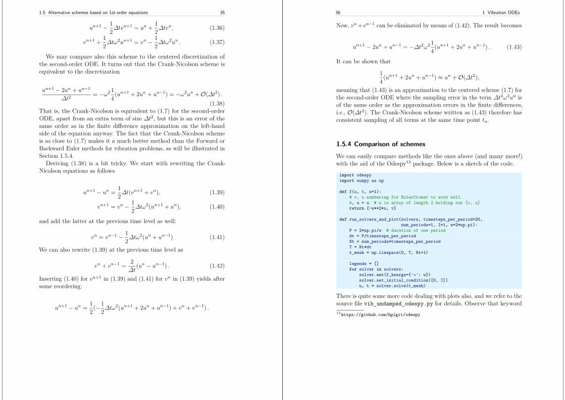
1.5 Alternative schemes based on 1st-order equations 35
un+1 − 12∆tv
n+1 = un + 12∆tv
n, (1.36)
vn+1 + 12∆tω
2un+1 = vn − 12∆tω
2un . (1.37)
We may compare also this scheme to the centered discretization ofthe second-order ODE. It turns out that the Crank-Nicolson scheme isequivalent to the discretization
un+1 − 2un + un−1
∆t2= −ω2 1
4(un+1 + 2un + un−1) = −ω2un +O(∆t2) .(1.38)
That is, the Crank-Nicolson is equivalent to (1.7) for the second-orderODE, apart from an extra term of size ∆t2, but this is an error of thesame order as in the finite difference approximation on the left-handside of the equation anyway. The fact that the Crank-Nicolson schemeis so close to (1.7) makes it a much better method than the Forward orBackward Euler methods for vibration problems, as will be illustrated inSection 1.5.4.
Deriving (1.38) is a bit tricky. We start with rewriting the Crank-Nicolson equations as follows
un+1 − un = 12∆t(v
n+1 + vn), (1.39)
vn+1 = vn − 12∆tω
2(un+1 + un), (1.40)
and add the latter at the previous time level as well:
vn = vn−1 − 12∆tω
2(un + un−1) (1.41)
We can also rewrite (1.39) at the previous time level as
vn + vn−1 = 2∆t
(un − un−1) . (1.42)
Inserting (1.40) for vn+1 in (1.39) and (1.41) for vn in (1.39) yields aftersome reordering:
un+1 − un = 12(−1
2∆tω2(un+1 + 2un + un−1) + vn + vn−1) .
36 1 Vibration ODEs
Now, vn+vn−1 can be eliminated by means of (1.42). The result becomes
un+1 − 2un + un−1 = −∆t2ω2 14(un+1 + 2un + un−1) . (1.43)
It can be shown that
14(un+1 + 2un + un−1) ≈ un +O(∆t2),
meaning that (1.43) is an approximation to the centered scheme (1.7) forthe second-order ODE where the sampling error in the term ∆t2ω2un isof the same order as the approximation errors in the finite differences,i.e., O(∆t2). The Crank-Nicolson scheme written as (1.43) therefore hasconsistent sampling of all terms at the same time point tn.
1.5.4 Comparison of schemes
We can easily compare methods like the ones above (and many more!)with the aid of the Odespy13 package. Below is a sketch of the code.
import odespyimport numpy as np
def f(u, t, w=1):# v, u numbering for EulerCromer to work wellv, u = u # u is array of length 2 holding our [v, u]return [-w**2*u, v]
def run_solvers_and_plot(solvers, timesteps_per_period=20,num_periods=1, I=1, w=2*np.pi):
P = 2*np.pi/w # duration of one perioddt = P/timesteps_per_periodNt = num_periods*timesteps_per_periodT = Nt*dtt_mesh = np.linspace(0, T, Nt+1)
legends = []for solver in solvers:
solver.set(f_kwargs=’w’: w)solver.set_initial_condition([0, I])u, t = solver.solve(t_mesh)
There is quite some more code dealing with plots also, and we refer to thesource file vib_undamped_odespy.py for details. Observe that keyword13 https://github.com/hplgit/odespy
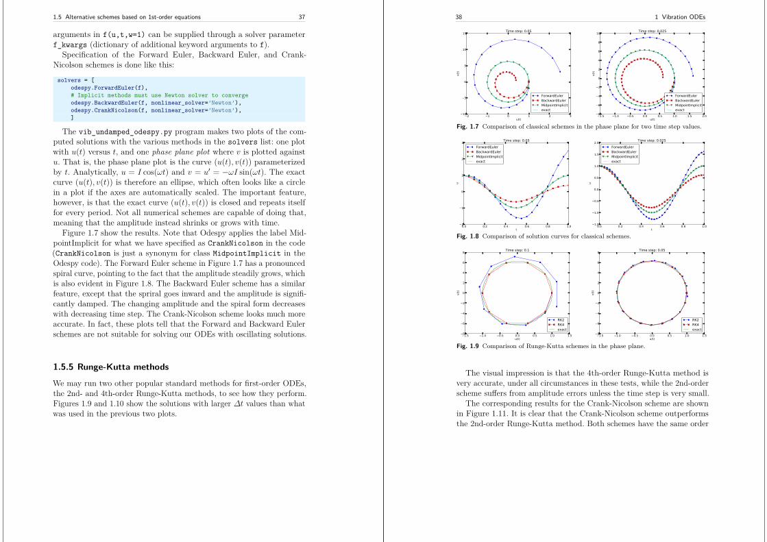
1.5 Alternative schemes based on 1st-order equations 37
arguments in f(u,t,w=1) can be supplied through a solver parameterf_kwargs (dictionary of additional keyword arguments to f).
Specification of the Forward Euler, Backward Euler, and Crank-Nicolson schemes is done like this:
solvers = [odespy.ForwardEuler(f),# Implicit methods must use Newton solver to convergeodespy.BackwardEuler(f, nonlinear_solver=’Newton’),odespy.CrankNicolson(f, nonlinear_solver=’Newton’),]
The vib_undamped_odespy.py program makes two plots of the com-puted solutions with the various methods in the solvers list: one plotwith u(t) versus t, and one phase plane plot where v is plotted againstu. That is, the phase plane plot is the curve (u(t), v(t)) parameterizedby t. Analytically, u = I cos(ωt) and v = u′ = −ωI sin(ωt). The exactcurve (u(t), v(t)) is therefore an ellipse, which often looks like a circlein a plot if the axes are automatically scaled. The important feature,however, is that the exact curve (u(t), v(t)) is closed and repeats itselffor every period. Not all numerical schemes are capable of doing that,meaning that the amplitude instead shrinks or grows with time.
Figure 1.7 show the results. Note that Odespy applies the label Mid-pointImplicit for what we have specified as CrankNicolson in the code(CrankNicolson is just a synonym for class MidpointImplicit in theOdespy code). The Forward Euler scheme in Figure 1.7 has a pronouncedspiral curve, pointing to the fact that the amplitude steadily grows, whichis also evident in Figure 1.8. The Backward Euler scheme has a similarfeature, except that the spriral goes inward and the amplitude is signifi-cantly damped. The changing amplitude and the spiral form decreaseswith decreasing time step. The Crank-Nicolson scheme looks much moreaccurate. In fact, these plots tell that the Forward and Backward Eulerschemes are not suitable for solving our ODEs with oscillating solutions.
1.5.5 Runge-Kutta methods
We may run two other popular standard methods for first-order ODEs,the 2nd- and 4th-order Runge-Kutta methods, to see how they perform.Figures 1.9 and 1.10 show the solutions with larger ∆t values than whatwas used in the previous two plots.
38 1 Vibration ODEs
2 1 0 1 2 3u(t)
10
5
0
5
10
15
v(t
)
Time step: 0.05
ForwardEulerBackwardEulerMidpointImplicitexact
1.5 1.0 0.5 0.0 0.5 1.0 1.5 2.0u(t)
8
6
4
2
0
2
4
6
8
10
v(t
)
Time step: 0.025
ForwardEulerBackwardEulerMidpointImplicitexact
Fig. 1.7 Comparison of classical schemes in the phase plane for two time step values.
0.0 0.2 0.4 0.6 0.8 1.0t
2
1
0
1
2
3
u
Time step: 0.05
ForwardEulerBackwardEulerMidpointImplicitexact
0.0 0.2 0.4 0.6 0.8 1.0t
1.5
1.0
0.5
0.0
0.5
1.0
1.5
2.0
u
Time step: 0.025
ForwardEulerBackwardEulerMidpointImplicitexact
Fig. 1.8 Comparison of solution curves for classical schemes.
1.5 1.0 0.5 0.0 0.5 1.0 1.5u(t)
8
6
4
2
0
2
4
6
8
v(t
)
Time step: 0.1
RK2RK4exact
1.5 1.0 0.5 0.0 0.5 1.0 1.5u(t)
8
6
4
2
0
2
4
6
8
v(t
)
Time step: 0.05
RK2RK4exact
Fig. 1.9 Comparison of Runge-Kutta schemes in the phase plane.
The visual impression is that the 4th-order Runge-Kutta method isvery accurate, under all circumstances in these tests, while the 2nd-orderscheme suffers from amplitude errors unless the time step is very small.
The corresponding results for the Crank-Nicolson scheme are shownin Figure 1.11. It is clear that the Crank-Nicolson scheme outperformsthe 2nd-order Runge-Kutta method. Both schemes have the same order
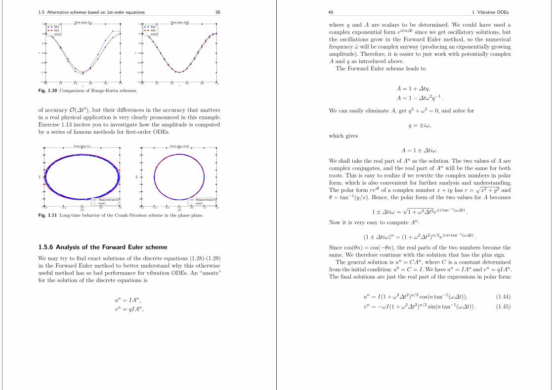
1.5 Alternative schemes based on 1st-order equations 39
0.0 0.2 0.4 0.6 0.8 1.0t
1.5
1.0
0.5
0.0
0.5
1.0
1.5
u
Time step: 0.1
RK2RK4exact
0.0 0.2 0.4 0.6 0.8 1.0t
1.5
1.0
0.5
0.0
0.5
1.0
1.5
u
Time step: 0.05
RK2RK4exact
Fig. 1.10 Comparison of Runge-Kutta schemes.
of accuracy O(∆t2), but their differences in the accuracy that mattersin a real physical application is very clearly pronounced in this example.Exercise 1.13 invites you to investigate how the amplitude is computedby a series of famous methods for first-order ODEs.
1.0 0.5 0.0 0.5 1.0u(t)
8
6
4
2
0
2
4
6
8
v(t
)
Time step: 0.1
MidpointImplicitexact
1.5 1.0 0.5 0.0 0.5 1.0 1.5u(t)
8
6
4
2
0
2
4
6
8
v(t
)
Time step: 0.05
MidpointImplicitexact
Fig. 1.11 Long-time behavior of the Crank-Nicolson scheme in the phase plane.
1.5.6 Analysis of the Forward Euler schemeWe may try to find exact solutions of the discrete equations (1.28)-(1.29)in the Forward Euler method to better understand why this otherwiseuseful method has so bad performance for vibration ODEs. An “ansatz”for the solution of the discrete equations is
un = IAn,
vn = qIAn,
40 1 Vibration ODEs
where q and A are scalars to be determined. We could have used acomplex exponential form eiωn∆t since we get oscillatory solutions, butthe oscillations grow in the Forward Euler method, so the numericalfrequency ω will be complex anyway (producing an exponentially growingamplitude). Therefore, it is easier to just work with potentially complexA and q as introduced above.
The Forward Euler scheme leads to
A = 1 +∆tq,
A = 1−∆tω2q−1 .
We can easily eliminate A, get q2 + ω2 = 0, and solve for
q = ±iω,which gives
A = 1±∆tiω .We shall take the real part of An as the solution. The two values of A arecomplex conjugates, and the real part of An will be the same for bothroots. This is easy to realize if we rewrite the complex numbers in polarform, which is also convenient for further analysis and understanding.The polar form reiθ of a complex number x+ iy has r =
√x2 + y2 and
θ = tan−1(y/x). Hence, the polar form of the two values for A becomes
1±∆tiω =√
1 + ω2∆t2e±i tan−1(ω∆t) .
Now it is very easy to compute An:
(1±∆tiω)n = (1 + ω2∆t2)n/2e±ni tan−1(ω∆t) .
Since cos(θn) = cos(−θn), the real parts of the two numbers become thesame. We therefore continue with the solution that has the plus sign.
The general solution is un = CAn, where C is a constant determinedfrom the initial condition: u0 = C = I. We have un = IAn and vn = qIAn.The final solutions are just the real part of the expressions in polar form:
un = I(1 + ω2∆t2)n/2 cos(n tan−1(ω∆t)), (1.44)vn = −ωI(1 + ω2∆t2)n/2 sin(n tan−1(ω∆t)) . (1.45)
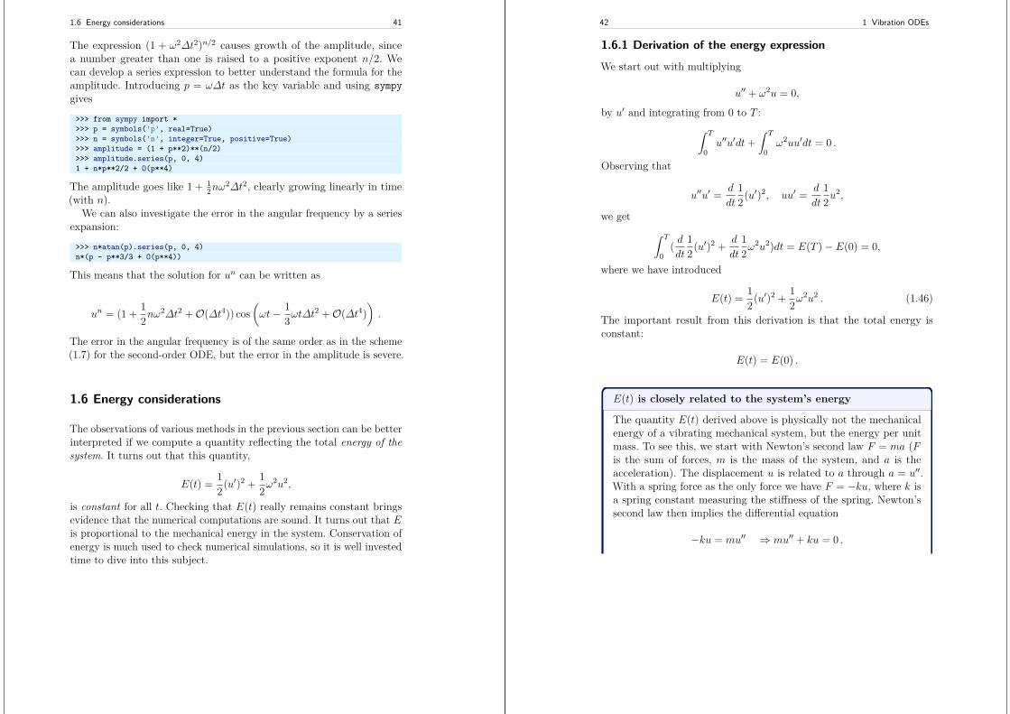
1.6 Energy considerations 41
The expression (1 + ω2∆t2)n/2 causes growth of the amplitude, sincea number greater than one is raised to a positive exponent n/2. Wecan develop a series expression to better understand the formula for theamplitude. Introducing p = ω∆t as the key variable and using sympygives
>>> from sympy import *>>> p = symbols(’p’, real=True)>>> n = symbols(’n’, integer=True, positive=True)>>> amplitude = (1 + p**2)**(n/2)>>> amplitude.series(p, 0, 4)1 + n*p**2/2 + O(p**4)
The amplitude goes like 1 + 12nω
2∆t2, clearly growing linearly in time(with n).
We can also investigate the error in the angular frequency by a seriesexpansion:
>>> n*atan(p).series(p, 0, 4)n*(p - p**3/3 + O(p**4))
This means that the solution for un can be written as
un = (1 + 12nω
2∆t2 +O(∆t4)) cos(ωt− 1
3ωt∆t2 +O(∆t4)
).
The error in the angular frequency is of the same order as in the scheme(1.7) for the second-order ODE, but the error in the amplitude is severe.
1.6 Energy considerations
The observations of various methods in the previous section can be betterinterpreted if we compute a quantity reflecting the total energy of thesystem. It turns out that this quantity,
E(t) = 12(u′)2 + 1
2ω2u2,
is constant for all t. Checking that E(t) really remains constant bringsevidence that the numerical computations are sound. It turns out that Eis proportional to the mechanical energy in the system. Conservation ofenergy is much used to check numerical simulations, so it is well investedtime to dive into this subject.
42 1 Vibration ODEs
1.6.1 Derivation of the energy expression
We start out with multiplying
u′′ + ω2u = 0,
by u′ and integrating from 0 to T :∫ T
0u′′u′dt+
∫ T
0ω2uu′dt = 0 .
Observing that
u′′u′ = d
dt
12(u′)2, uu′ = d
dt
12u
2,
we get∫ T
0( ddt
12(u′)2 + d
dt
12ω
2u2)dt = E(T )− E(0) = 0,
where we have introduced
E(t) = 12(u′)2 + 1
2ω2u2 . (1.46)
The important result from this derivation is that the total energy isconstant:
E(t) = E(0) .
E(t) is closely related to the system’s energy
The quantity E(t) derived above is physically not the mechanicalenergy of a vibrating mechanical system, but the energy per unitmass. To see this, we start with Newton’s second law F = ma (Fis the sum of forces, m is the mass of the system, and a is theacceleration). The displacement u is related to a through a = u′′.With a spring force as the only force we have F = −ku, where k isa spring constant measuring the stiffness of the spring. Newton’ssecond law then implies the differential equation
−ku = mu′′ ⇒ mu′′ + ku = 0 .
1.6 Energy considerations 43
This equation of motion can be turned into an energy balanceequation by finding the work done by each term during a timeinterval [0, T ]. To this end, we multiply the equation by du = u′dtand integrate:
∫ T
0muu′dt+
∫ T
0kuu′dt = 0 .
The result is
E(t) = Ek(t) + Ep(t) = 0,
where
Ek(t) = 12mv
2, v = u′, (1.47)
is the kinetic energy of the system, and
Ep(t) = 12ku
2 (1.48)
is the potential energy. The sum E(t) is the total mechanical energy.The derivation demonstrates the famous energy principle that, underthe right physical circumstances, any change in the kinetic energy isdue to a change in potential energy and vice versa. (This principlebreaks down when we introduce damping in the system, as we doin Section 1.10.)
The equation mu′′ + ku = 0 can be divided by m and writtenas u′′ + ω2u = 0 for ω =
√k/m. The energy expression E(t) =
12(u′)2+ 1
2ω2u2 derived earlier is then E(t)/m, i.e., mechanical energy
per unit mass.
Energy of the exact solution. Analytically, we have u(t) = I cosωt, ifu(0) = I and u′(0) = 0, so we can easily check the energy evolution andconfirm that E(t) is constant:
E(t) = 12I
2(−ω sinωt)2+ 12ω
2I2 cos2 ωt = 12ω
2(sin2 ωt+cos2 ωt) = 12ω
2 .
Growth of energy in the Forward Euler scheme. The energy at timelevel n+ 1 in the Forward Euler scheme can easily be shown to increase:
44 1 Vibration ODEs
En+1 = 12(vn+1)2 + 1
2ω2(un+1)2
= 12(vn − ω2∆tun)2 + 1
2ω2(un +∆tvn)2
= (1 +∆t2ω2)En .
1.6.2 An error measure based on energyThe constant energy is well expressed by its initial value E(0), so thatthe error in mechanical energy can be computed as a mesh function by
enE = 12
(un+1 − un−1
2∆t
)2
+ 12ω
2(un)2−E(0), n = 1, . . . , Nt−1, (1.49)
where
E(0) = 12V
2 + 12ω
2I2,
if u(0) = I and u′(0) = V . Note that we have used a centered approxi-mation to u′: u′(tn) ≈ [D2tu]n.
A useful norm of the mesh function enE for the discrete mechanicalenergy can be the maximum absolute value of enE :
||enE ||`∞ = max1≤n<Nt
|enE | .
Alternatively, we can compute other norms involving integration over allmesh points, but we are often interested in worst case deviation of theenergy, and then the maximum value is of particular relevance.
A vectorized Python implementation of enE takes the form
# import numpy as np and compute u, tdt = t[1]-t[0]E = 0.5*((u[2:] - u[:-2])/(2*dt))**2 + 0.5*w**2*u[1:-1]**2E0 = 0.5*V**2 + 0.5**w**2*I**2e_E = E - E0e_E_norm = np.abs(e_E).max()
The convergence rates of the quantity e_E_norm can be used forverification. The value of e_E_norm is also useful for comparing schemesthrough their ability to preserve energy. Below is a table demonstratingthe relative error in total energy for various schemes (computed by thevib_undamped_odespy.py program). The test problem is u′′ + 4π2u = 0
1.6 Energy considerations 45
with u(0) = 1 and u′(0) = 0, so the period is 1 and E(t) ≈ 4.93. Weclearly see that the Crank-Nicolson and the Runge-Kutta schemes aresuperior to the Forward and Backward Euler schemes already after oneperiod.
Method T ∆t max |enE | /e0E
Forward Euler 1 0.025 1.678 · 100
Backward Euler 1 0.025 6.235 · 10−1
Crank-Nicolson 1 0.025 1.221 · 10−2
Runge-Kutta 2nd-order 1 0.025 6.076 · 10−3
Runge-Kutta 4th-order 1 0.025 8.214 · 10−3
However, after 10 periods, the picture is much more dramatic:
Method T ∆t max |enE | /e0E
Forward Euler 10 0.025 1.788 · 104
Backward Euler 10 0.025 1.000 · 100
Crank-Nicolson 10 0.025 1.221 · 10−2
Runge-Kutta 2nd-order 10 0.025 6.250 · 10−2
Runge-Kutta 4th-order 10 0.025 8.288 · 10−3
The Runge-Kutta and Crank-Nicolson methods hardly change theirenergy error with T , while the error in the Forward Euler method growsto huge levels and a relative error of 1 in the Backward Euler methodpoints to E(t)→ 0 as t grows large.
Running multiple values of ∆t, we can get some insight into theconvergence of the energy error:
Method T ∆t max |enE | /e0E
Forward Euler 10 0.05 1.120 · 108
Forward Euler 10 0.025 1.788 · 104
Forward Euler 10 0.0125 1.374 · 102
Backward Euler 10 0.05 1.000 · 100
Backward Euler 10 0.025 1.000 · 100
Backward Euler 10 0.0125 9.928 · 10−1
Crank-Nicolson 10 0.05 4.756 · 10−2
Crank-Nicolson 10 0.025 1.221 · 10−2
Crank-Nicolson 10 0.0125 3.125 · 10−3
Runge-Kutta 2nd-order 10 0.05 6.152 · 10−1
Runge-Kutta 2nd-order 10 0.025 6.250 · 10−2
Runge-Kutta 2nd-order 10 0.0125 7.631 · 10−3
Runge-Kutta 4th-order 10 0.05 3.510 · 10−2
Runge-Kutta 4th-order 10 0.025 8.288 · 10−3
Runge-Kutta 4th-order 10 0.0125 2.058 · 10−3
A striking fact from this table is that the error of the Forward Eulermethod is reduced by the same factor as ∆t is reduced by, while the
46 1 Vibration ODEs
error in the Crank-Nicolson method has a reduction proportional to ∆t2(we cannot say anything for the Backward Euler method). However, forthe RK2 method, halving ∆t reduces the error by almost a factor of 10(!), and for the RK4 method the reduction seems proportional to ∆t2only (and the trend is confirmed by running smaller time steps, so for∆t = 3.9 · 10−4 the relative error of RK2 is a factor 10 smaller than thatof RK4!).
1.7 The Euler-Cromer method
While the Runge-Kutta methods and the Crank-Nicolson scheme workwell for the vibration equation modeled as a first-order ODE system,both were inferior to the straightforward centered difference scheme forthe second-order equation u′′ + ω2u = 0. However, there is a similarlysuccessful scheme available for the first-order system u′ = v, v′ = −ω2u,to be presented below. The ideas of the scheme and their further devel-opments have become very popular in particle and rigid body dynamicsand hence widely used by physicists.
1.7.1 Forward-backward discretization
The idea is to apply a Forward Euler discretization to the first equationand a Backward Euler discretization to the second. In operator notationthis is stated as
[D+t u = v]n, (1.50)
[D−t v = −ω2u]n+1 . (1.51)
We can write out the formulas and collect the unknowns on the left-handside:
un+1 = un +∆tvn, (1.52)vn+1 = vn −∆tω2un+1 . (1.53)
We realize that after un+1 has been computed from (1.52), it may beused directly in (1.53) to compute vn+1.
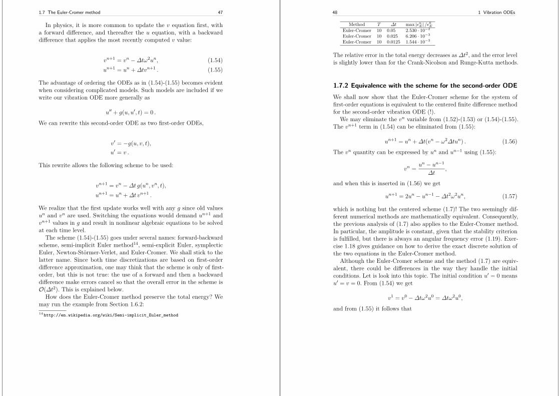
1.7 The Euler-Cromer method 47
In physics, it is more common to update the v equation first, witha forward difference, and thereafter the u equation, with a backwarddifference that applies the most recently computed v value:
vn+1 = vn −∆tω2un, (1.54)un+1 = un +∆tvn+1 . (1.55)
The advantage of ordering the ODEs as in (1.54)-(1.55) becomes evidentwhen considering complicated models. Such models are included if wewrite our vibration ODE more generally as
u′′ + g(u, u′, t) = 0 .
We can rewrite this second-order ODE as two first-order ODEs,
v′ = −g(u, v, t),u′ = v .
This rewrite allows the following scheme to be used:
vn+1 = vn −∆t g(un, vn, t),un+1 = un +∆t vn+1 .
We realize that the first update works well with any g since old valuesun and vn are used. Switching the equations would demand un+1 andvn+1 values in g and result in nonlinear algebraic equations to be solvedat each time level.
The scheme (1.54)-(1.55) goes under several names: forward-backwardscheme, semi-implicit Euler method14, semi-explicit Euler, symplecticEuler, Newton-Störmer-Verlet, and Euler-Cromer. We shall stick to thelatter name. Since both time discretizations are based on first-orderdifference approximation, one may think that the scheme is only of first-order, but this is not true: the use of a forward and then a backwarddifference make errors cancel so that the overall error in the scheme isO(∆t2). This is explained below.
How does the Euler-Cromer method preserve the total energy? Wemay run the example from Section 1.6.2:14 http://en.wikipedia.org/wiki/Semi-implicit_Euler_method
48 1 Vibration ODEs
Method T ∆t max |enE | /e0E
Euler-Cromer 10 0.05 2.530 · 10−2
Euler-Cromer 10 0.025 6.206 · 10−3
Euler-Cromer 10 0.0125 1.544 · 10−3
The relative error in the total energy decreases as ∆t2, and the error levelis slightly lower than for the Crank-Nicolson and Runge-Kutta methods.
1.7.2 Equivalence with the scheme for the second-order ODEWe shall now show that the Euler-Cromer scheme for the system offirst-order equations is equivalent to the centered finite difference methodfor the second-order vibration ODE (!).
We may eliminate the vn variable from (1.52)-(1.53) or (1.54)-(1.55).The vn+1 term in (1.54) can be eliminated from (1.55):
un+1 = un +∆t(vn − ω2∆tun) . (1.56)
The vn quantity can be expressed by un and un−1 using (1.55):
vn = un − un−1
∆t,
and when this is inserted in (1.56) we get
un+1 = 2un − un−1 −∆t2ω2un, (1.57)
which is nothing but the centered scheme (1.7)! The two seemingly dif-ferent numerical methods are mathematically equivalent. Consequently,the previous analysis of (1.7) also applies to the Euler-Cromer method.In particular, the amplitude is constant, given that the stability criterionis fulfilled, but there is always an angular frequency error (1.19). Exer-cise 1.18 gives guidance on how to derive the exact discrete solution ofthe two equations in the Euler-Cromer method.
Although the Euler-Cromer scheme and the method (1.7) are equiv-alent, there could be differences in the way they handle the initialconditions. Let is look into this topic. The initial condition u′ = 0 meansu′ = v = 0. From (1.54) we get
v1 = v0 −∆tω2u0 = ∆tω2u0,
and from (1.55) it follows that
1.7 The Euler-Cromer method 49
u1 = u0 +∆tv1 = u0 − ω2∆t2u0 .
When we previously used a centered approximation of u′(0) = 0 combinedwith the discretization (1.7) of the second-order ODE, we got a slightlydifferent result: u1 = u0 − 1
2ω2∆t2u0. The difference is 1
2ω2∆t2u0, which
is of second order in ∆t, seemingly consistent with the overall error inthe scheme for the differential equation model.
A different view can also be taken. If we approximate u′(0) = 0 bya backward difference, (u0 − u−1)/∆t = 0, we get u−1 = u0, and whencombined with (1.7), it results in u1 = u0 − ω2∆t2u0. This means thatthe Euler-Cromer method based on (1.55)-(1.54) corresponds to usingonly a first-order approximation to the initial condition in the methodfrom Section 1.1.2.
Correspondingly, using the formulation (1.52)-(1.53) with vn = 0leads to u1 = u0, which can be interpreted as using a forward differenceapproximation for the initial condition u′(0) = 0. Both Euler-Cromerformulations lead to slightly different values for u1 compared to themethod in Section 1.1.2. The error is 1
2ω2∆t2u0.
1.7.3 ImplementationSolver function. The function below, found in vib_undamped_EulerCromer.py, implements the Euler-Cromer scheme (1.54)-(1.55):
import numpy as np
def solver(I, w, dt, T):"""Solve v’ = - w**2*u, u’=v for t in (0,T], u(0)=I and v(0)=0,by an Euler-Cromer method."""dt = float(dt)Nt = int(round(T/dt))u = np.zeros(Nt+1)v = np.zeros(Nt+1)t = np.linspace(0, Nt*dt, Nt+1)
v[0] = 0u[0] = Ifor n in range(0, Nt):
v[n+1] = v[n] - dt*w**2*u[n]u[n+1] = u[n] + dt*v[n+1]
return u, v, t
Verification. Since the Euler-Cromer scheme is equivalent to the finitedifference method for the second-order ODE u′′ + ω2u = 0 (see Sec-
50 1 Vibration ODEs
tion 1.7.2), the performance of the above solver function is the same asfor the solver function in Section 1.2. The only difference is the formulafor the first time step, as discussed above. This deviation in the Euler-Cromer scheme means that the discrete solution listed in Section 1.4.4 isnot a solution of the Euler-Cromer scheme!
To verify the implementation of the Euler-Cromer method we canadjust v[1] so that the computer-generated values can be comparedwith the formula (1.20) from in Section 1.4.4. This adjustment is done inan alternative solver function, solver_ic_fix in vib_EulerCromer.py.Since we now have an exact solution of the discrete equations available,we can write a test function test_solver for checking the equality ofcomputed values with the formula (1.20):
def test_solver():"""Test solver with fixed initial condition againstequivalent scheme for the 2nd-order ODE u’’ + u = 0."""I = 1.2; w = 2.0; T = 5dt = 2/w # longest possible time stepu, v, t = solver_ic_fix(I, w, dt, T)from vib_undamped import solver as solver2 # 2nd-order ODEu2, t2 = solver2(I, w, dt, T)error = np.abs(u - u2).max()tol = 1E-14assert error < tol
Another function, demo, visualizes the difference between the Euler-Cromer scheme and the scheme (1.7) for the second-oder ODE, arisingfrom the mismatch in the first time level.
Using Odespy. The Euler-Cromer method is also available in the Odespypackage. The important thing to remember, when using this implemen-tation, is that we must order the unknowns as v and u, so the u vectorat each time level consists of the velocity v as first component and thedisplacement u as second component:
# Define ODEdef f(u, t, w=1):
v, u = ureturn [-w**2*u, v]
# Initialize solverI = 1w = 2*np.piimport odespysolver = odespy.EulerCromer(f, f_kwargs=’w’: w)solver.set_initial_condition([0, I])
1.7 The Euler-Cromer method 51
# Compute time meshP = 2*np.pi/w # duration of one perioddt = P/timesteps_per_periodNt = num_periods*timesteps_per_periodT = Nt*dtimport numpy as npt_mesh = np.linspace(0, T, Nt+1)
# Solve ODEu, t = solver.solve(t_mesh)u = u[:,1] # Extract displacement
Convergence rates. We may use the convergence_rates function inthe file vib_undamped.py to investigate the convergence rate of theEuler-Cromer method, see the convergence_rate function in the filevib_undamped_EulerCromer.py. Since we could eliminate v to get ascheme for u that is equivalent to the finite difference method for thesecond-order equation in u, we would expect the convergence rates tobe the same, i.e., O(∆t2). However, measuring the convergence rate ofu in the Euler-Cromer scheme shows that it is O(∆t)! Adjusting theinitial condition does not change the rate. Adjusting ω, as outlined inSection 1.4.2, gives a 4th-order method there, while there is no increasein the measured rate in the Euler-Cromer scheme. It is obvious that theEuler-Cromer scheme is dramatically much better than the two otherfirst-order methods, Forward Euler and Backward Euler, but this is notreflected in the convergence rate of u.
1.7.4 The Störmer-Verlet algorithmAnother very popular algorithm for vibration problems, especially forlong time simulations, is the Stömer-Verlet algorithm. It has become themethod among physicists for molecular simulations as well as particleand rigid body dynamics.
The method can be derived by applying the Euler-Cromer idea twice,in a symmetric fashion, during the interval [tn, tn+1]:
1. solve v′ = −ωu by a Forward Euler step in [tn, tn+ 12]
2. solve u′ = v by a Backward Euler step in [tn, tn+ 12]
3. solve u′ = v by a Forward Euler step in [tn+ 12, tn+1]
4. solve v′ = −ωu by a Backward Euler step in [tn+ 12, tn+1]
With mathematics,
52 1 Vibration ODEs
vn+ 12 − vn
12∆t
= −ω2un,
un+ 12 − un
12∆t
= vn+ 12 ,
un+1 − un− 12
12∆t
= vn+ 12 ,
vn+1 − vn+ 12
12∆t
= −ω2un+1 .
The two steps in the middle can be combined to
un+1 − un−1
∆t= vn+ 1
2 ,
and consequently
vn+ 12 = vn − 1
2∆tω2un, (1.58)
un+1 = un +∆tvn+ 12 , (1.59)
vn+1 = vn+ 12 − 1
2∆tω2un+1 . (1.60)
Writing the last equation as vn = vn−12 − 1
2∆tω2un and using this vn in
the first equation gives vn+ 12 = vn−
12 −∆tω2un, and the scheme can be
written as two steps:
vn+ 12 = vn−
12 −∆tω2un, (1.61)
un+1 = un +∆tvn+ 12 , (1.62)
which is nothing but straightforward centered differences for the 2× 2ODE system on a staggered mesh, see Section 1.8.1. We have thusseen that four different reasonings (discretizing u′′ + ω2u directly, usingEuler-Cromer, using Stömer-Verlet, and using centered differences for the2times2 system on a staggered mesh) all end up with the same equations!The main difference is that the traditional Euler-Cromer displays first-
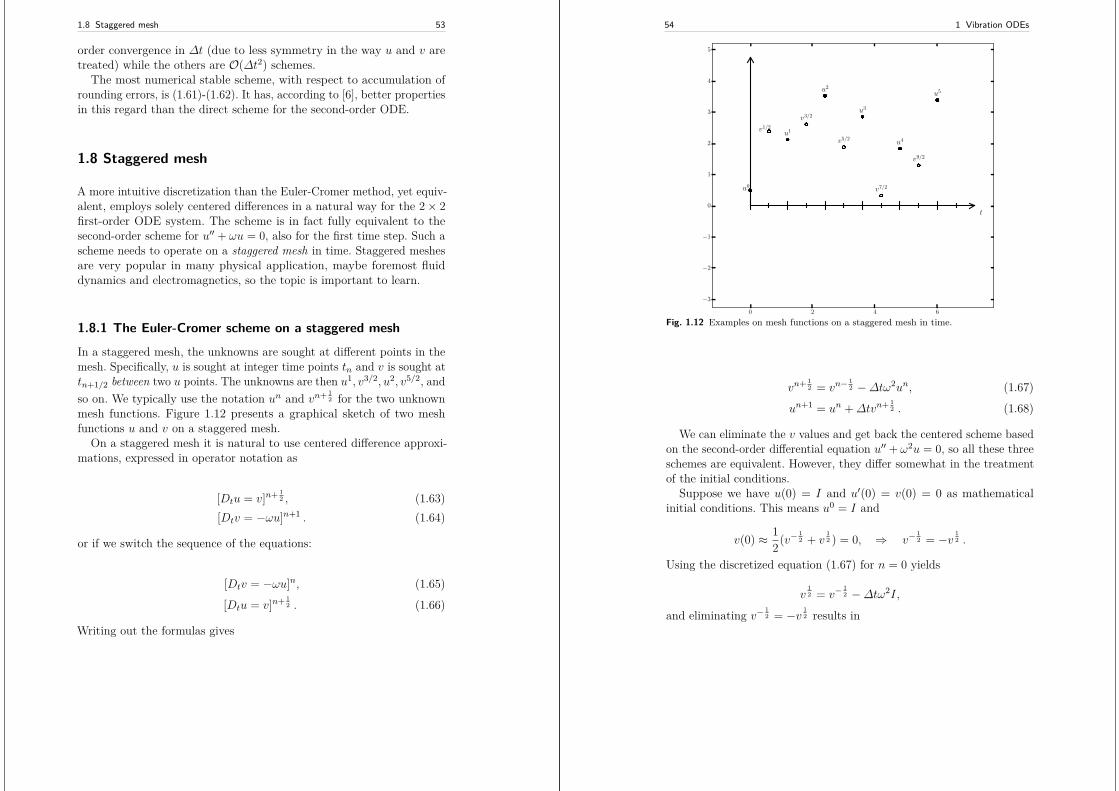
1.8 Staggered mesh 53
order convergence in ∆t (due to less symmetry in the way u and v aretreated) while the others are O(∆t2) schemes.
The most numerical stable scheme, with respect to accumulation ofrounding errors, is (1.61)-(1.62). It has, according to [6], better propertiesin this regard than the direct scheme for the second-order ODE.
1.8 Staggered mesh
A more intuitive discretization than the Euler-Cromer method, yet equiv-alent, employs solely centered differences in a natural way for the 2× 2first-order ODE system. The scheme is in fact fully equivalent to thesecond-order scheme for u′′ + ωu = 0, also for the first time step. Such ascheme needs to operate on a staggered mesh in time. Staggered meshesare very popular in many physical application, maybe foremost fluiddynamics and electromagnetics, so the topic is important to learn.
1.8.1 The Euler-Cromer scheme on a staggered mesh
In a staggered mesh, the unknowns are sought at different points in themesh. Specifically, u is sought at integer time points tn and v is sought attn+1/2 between two u points. The unknowns are then u1, v3/2, u2, v5/2, andso on. We typically use the notation un and vn+ 1
2 for the two unknownmesh functions. Figure 1.12 presents a graphical sketch of two meshfunctions u and v on a staggered mesh.
On a staggered mesh it is natural to use centered difference approxi-mations, expressed in operator notation as
[Dtu = v]n+ 12 , (1.63)
[Dtv = −ωu]n+1 . (1.64)
or if we switch the sequence of the equations:
[Dtv = −ωu]n, (1.65)[Dtu = v]n+ 1
2 . (1.66)
Writing out the formulas gives
54 1 Vibration ODEs
0 2 4 6
−3
−2
−1
0
1
2
3
4
5
t
u0
u1
u2
u3
u4
u5
v1/2
v3/2
v5/2
v7/2
v9/2
Fig. 1.12 Examples on mesh functions on a staggered mesh in time.
vn+ 12 = vn−
12 −∆tω2un, (1.67)
un+1 = un +∆tvn+ 12 . (1.68)
We can eliminate the v values and get back the centered scheme basedon the second-order differential equation u′′ + ω2u = 0, so all these threeschemes are equivalent. However, they differ somewhat in the treatmentof the initial conditions.
Suppose we have u(0) = I and u′(0) = v(0) = 0 as mathematicalinitial conditions. This means u0 = I and
v(0) ≈ 12(v− 1
2 + v12 ) = 0, ⇒ v−
12 = −v 1
2 .
Using the discretized equation (1.67) for n = 0 yields
v12 = v−
12 −∆tω2I,
and eliminating v− 12 = −v 1
2 results in
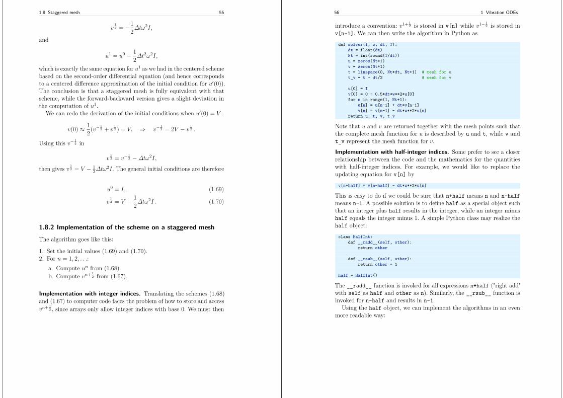
1.8 Staggered mesh 55
v12 = −1
2∆tω2I,
and
u1 = u0 − 12∆t
2ω2I,
which is exactly the same equation for u1 as we had in the centered schemebased on the second-order differential equation (and hence correspondsto a centered difference approximation of the initial condition for u′(0)).The conclusion is that a staggered mesh is fully equivalent with thatscheme, while the forward-backward version gives a slight deviation inthe computation of u1.
We can redo the derivation of the initial conditions when u′(0) = V :
v(0) ≈ 12(v− 1
2 + v12 ) = V, ⇒ v−
12 = 2V − v 1
2 .
Using this v− 12 in
v12 = v−
12 −∆tω2I,
then gives v 12 = V − 1
2∆tω2I. The general initial conditions are therefore
u0 = I, (1.69)
v12 = V − 1
2∆tω2I . (1.70)
1.8.2 Implementation of the scheme on a staggered mesh
The algorithm goes like this:
1. Set the initial values (1.69) and (1.70).2. For n = 1, 2, . . .:
a. Compute un from (1.68).b. Compute vn+ 1
2 from (1.67).
Implementation with integer indices. Translating the schemes (1.68)and (1.67) to computer code faces the problem of how to store and accessvn+ 1
2 , since arrays only allow integer indices with base 0. We must then
56 1 Vibration ODEs
introduce a convention: v1+ 12 is stored in v[n] while v1− 1
2 is stored inv[n-1]. We can then write the algorithm in Python as
def solver(I, w, dt, T):dt = float(dt)Nt = int(round(T/dt))u = zeros(Nt+1)v = zeros(Nt+1)t = linspace(0, Nt*dt, Nt+1) # mesh for ut_v = t + dt/2 # mesh for v
u[0] = Iv[0] = 0 - 0.5*dt*w**2*u[0]for n in range(1, Nt+1):
u[n] = u[n-1] + dt*v[n-1]v[n] = v[n-1] - dt*w**2*u[n]
return u, t, v, t_v
Note that u and v are returned together with the mesh points such thatthe complete mesh function for u is described by u and t, while v andt_v represent the mesh function for v.
Implementation with half-integer indices. Some prefer to see a closerrelationship between the code and the mathematics for the quantitieswith half-integer indices. For example, we would like to replace theupdating equation for v[n] by
v[n+half] = v[n-half] - dt*w**2*u[n]
This is easy to do if we could be sure that n+half means n and n-halfmeans n-1. A possible solution is to define half as a special object suchthat an integer plus half results in the integer, while an integer minushalf equals the integer minus 1. A simple Python class may realize thehalf object:
class HalfInt:def __radd__(self, other):
return other
def __rsub__(self, other):return other - 1
half = HalfInt()
The __radd__ function is invoked for all expressions n+half ("right add"with self as half and other as n). Similarly, the __rsub__ function isinvoked for n-half and results in n-1.
Using the half object, we can implement the algorithms in an evenmore readable way:
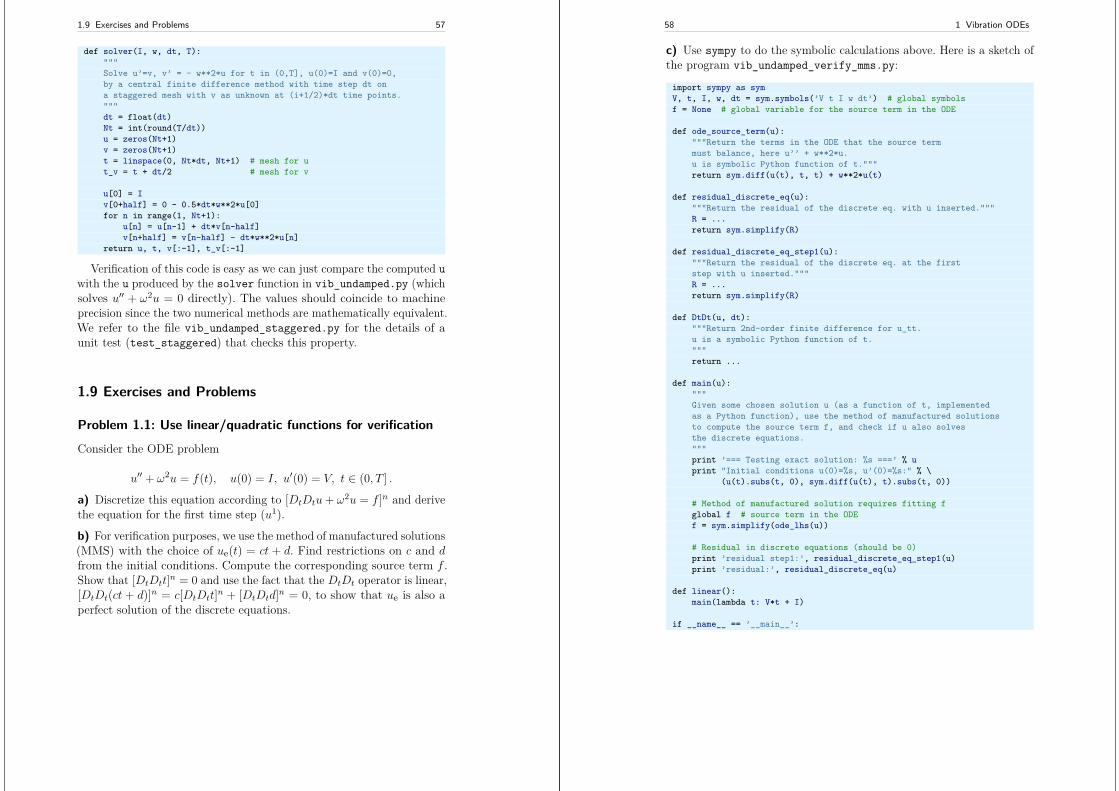
1.9 Exercises and Problems 57
def solver(I, w, dt, T):"""Solve u’=v, v’ = - w**2*u for t in (0,T], u(0)=I and v(0)=0,by a central finite difference method with time step dt ona staggered mesh with v as unknown at (i+1/2)*dt time points."""dt = float(dt)Nt = int(round(T/dt))u = zeros(Nt+1)v = zeros(Nt+1)t = linspace(0, Nt*dt, Nt+1) # mesh for ut_v = t + dt/2 # mesh for v
u[0] = Iv[0+half] = 0 - 0.5*dt*w**2*u[0]for n in range(1, Nt+1):
u[n] = u[n-1] + dt*v[n-half]v[n+half] = v[n-half] - dt*w**2*u[n]
return u, t, v[:-1], t_v[:-1]
Verification of this code is easy as we can just compare the computed uwith the u produced by the solver function in vib_undamped.py (whichsolves u′′ + ω2u = 0 directly). The values should coincide to machineprecision since the two numerical methods are mathematically equivalent.We refer to the file vib_undamped_staggered.py for the details of aunit test (test_staggered) that checks this property.
1.9 Exercises and Problems
Problem 1.1: Use linear/quadratic functions for verification
Consider the ODE problem
u′′ + ω2u = f(t), u(0) = I, u′(0) = V, t ∈ (0, T ] .
a) Discretize this equation according to [DtDtu+ ω2u = f ]n and derivethe equation for the first time step (u1).
b) For verification purposes, we use the method of manufactured solutions(MMS) with the choice of ue(t) = ct + d. Find restrictions on c and dfrom the initial conditions. Compute the corresponding source term f .Show that [DtDtt]n = 0 and use the fact that the DtDt operator is linear,[DtDt(ct + d)]n = c[DtDtt]n + [DtDtd]n = 0, to show that ue is also aperfect solution of the discrete equations.
58 1 Vibration ODEs
c) Use sympy to do the symbolic calculations above. Here is a sketch ofthe program vib_undamped_verify_mms.py:
import sympy as symV, t, I, w, dt = sym.symbols(’V t I w dt’) # global symbolsf = None # global variable for the source term in the ODE
def ode_source_term(u):"""Return the terms in the ODE that the source termmust balance, here u’’ + w**2*u.u is symbolic Python function of t."""return sym.diff(u(t), t, t) + w**2*u(t)
def residual_discrete_eq(u):"""Return the residual of the discrete eq. with u inserted."""R = ...return sym.simplify(R)
def residual_discrete_eq_step1(u):"""Return the residual of the discrete eq. at the firststep with u inserted."""R = ...return sym.simplify(R)
def DtDt(u, dt):"""Return 2nd-order finite difference for u_tt.u is a symbolic Python function of t."""return ...
def main(u):"""Given some chosen solution u (as a function of t, implementedas a Python function), use the method of manufactured solutionsto compute the source term f, and check if u also solvesthe discrete equations."""print ’=== Testing exact solution: %s ===’ % uprint "Initial conditions u(0)=%s, u’(0)=%s:" % \
(u(t).subs(t, 0), sym.diff(u(t), t).subs(t, 0))
# Method of manufactured solution requires fitting fglobal f # source term in the ODEf = sym.simplify(ode_lhs(u))
# Residual in discrete equations (should be 0)print ’residual step1:’, residual_discrete_eq_step1(u)print ’residual:’, residual_discrete_eq(u)
def linear():main(lambda t: V*t + I)
if __name__ == ’__main__’:
1.9 Exercises and Problems 59
linear()
Fill in the various functions such that the calls in the main functionworks.
d) The purpose now is to choose a quadratic function ue = bt2 +ct+d asexact solution. Extend the sympy code above with a function quadraticfor fitting f and checking if the discrete equations are fulfilled. (Thefunction is very similar to linear.)
e) Will a polynomial of degree three fulfill the discrete equations?
f) Implement a solver function for computing the numerical solutionof this problem.
g) Write a test function for checking that the quadratic solution is com-puted correctly (to machine precision, but the round-off errors accumulateand increase with T ) by the solver function.Filename: vib_undamped_verify_mms.
Exercise 1.2: Show linear growth of the phase with time
Consider an exact solution I cos(ωt) and an approximation I cos(ωt).Define the phase error as the time lag between the peak I in the exactsolution and the corresponding peak in the approximation afterm periodsof oscillations. Show that this phase error is linear in m.Filename: vib_phase_error_growth.
Exercise 1.3: Improve the accuracy by adjusting thefrequency
According to (1.19), the numerical frequency deviates from the exactfrequency by a (dominating) amount ω3∆t2/24 > 0. Replace the wparameter in the algorithm in the solver function in vib_undamped.pyby w*(1 - (1./24)*w**2*dt**2 and test how this adjustment in thenumerical algorithm improves the accuracy (use ∆t = 0.1 and simulatefor 80 periods, with and without adjustment of ω).Filename: vib_adjust_w.
60 1 Vibration ODEs
Exercise 1.4: See if adaptive methods improve the phaseerrorAdaptive methods for solving ODEs aim at adjusting ∆t such thatthe error is within a user-prescribed tolerance. Implement the equa-tion u′′ + u = 0 in the Odespy15 software. Use the example from Sec-tion 3.2.11 in [9]. Run the scheme with a very low tolerance (say 10−14)and for a long time, check the number of time points in the solver’s mesh(len(solver.t_all)), and compare the phase error with that producedby the simple finite difference method from Section 1.1.2 with the samenumber of (equally spaced) mesh points. The question is whether it paysoff to use an adaptive solver or if equally many points with a simplemethod gives about the same accuracy.Filename: vib_undamped_adaptive.
Exercise 1.5: Use a Taylor polynomial to compute u1
As an alternative to computing u1 by (1.8), one can use a Taylor polyno-mial with three terms:
u(t1) ≈ u(0) + u′(0)∆t+ 12u′′(0)∆t2
With u′′ = −ω2u and u′(0) = 0, show that this method also leads to(1.8). Generalize the condition on u′(0) to be u′(0) = V and compute u1
in this case with both methods.Filename: vib_first_step.
Problem 1.6: Derive and investigate the velocity VerletmethodThe velocity Verlet method for u′′ + ω2u = 0 is based on the followingideas:
1. step u forward from tn to tn+1 using a three-term Taylor series,2. replace u′′ by −ω2u3. discretize v′ = −ω2u by a Crank-Nicolson method.
Derive the scheme, implement it, and determine empirically the conver-gence rate.15 https://github.com/hplgit/odespy
1.9 Exercises and Problems 61
Problem 1.7: Find the minimal resolution of an oscillatoryfunctionSketch the function on a given mesh which has the highest possiblefrequency. That is, this oscillatory “cos-like” function has its maxima andminima at every two grid points. Find an expression for the frequency ofthis function, and use the result to find the largest relevant value of ω∆twhen ω is the frequency of an oscillating function and ∆t is the meshspacing.Filename: vib_largest_wdt.
Exercise 1.8: Visualize the accuracy of finite differences for acosine functionWe introduce the error fraction
E = [DtDtu]nu′′(tn)
to measure the error in the finite difference approximation DtDtu to u′′.Compute E for the specific choice of a cosine/sine function of the formu = exp (iωt) and show that
E =( 2ω∆t
)2sin2(ω∆t2 ) .
Plot E as a function of p = ω∆t. The relevant values of p are [0, π] (seeExercise 1.7 for why p > π does not make sense). The deviation of thecurve from unity visualizes the error in the approximation. Also expandE as a Taylor polynomial in p up to fourth degree (use, e.g., sympy).Filename: vib_plot_fd_exp_error.
Exercise 1.9: Verify convergence rates of the error in energyWe consider the ODE problem u′′ + ω2u = 0, u(0) = I, u′(0) = V , fort ∈ (0, T ]. The total energy of the solution E(t) = 1
2(u′)2 + 12ω
2u2 shouldstay constant. The error in energy can be computed as explained inSection 1.6.
Make a test function in a separate file, where code fromvib_undamped.py is imported, but the convergence_rates andtest_convergence_rates functions are copied and modified to also
62 1 Vibration ODEs
incorporate computations of the error in energy and the convergencerate of this error. The expected rate is 2, just as for the solution itself.Filename: test_error_conv.
Exercise 1.10: Use linear/quadratic functions for verification
This exercise is a generalization of Problem 1.1 to the extended modelproblem (1.71) where the damping term is either linear or quadratic.Solve the various subproblems and see how the results and problemsettings change with the generalized ODE in case of linear or quadraticdamping. By modifying the code from Problem 1.1, sympy will do mostof the work required to analyze the generalized problem.Filename: vib_verify_mms.
Exercise 1.11: Use an exact discrete solution for verification
Write a test function in a separate file that employs the exact discretesolution (1.20) to verify the implementation of the solver function inthe file vib_undamped.py.Filename: test_vib_undamped_exact_discrete_sol.
Exercise 1.12: Use analytical solution for convergence ratetests
The purpose of this exercise is to perform convergence tests of the problem(1.71) when s(u) = cu, F (t) = A sinφt and there is no damping. Find thecomplete analytical solution to the problem in this case (most textbookson mechanics or ordinary differential equations list the various elementsyou need to write down the exact solution, or you can use symbolictools like sympy or wolframalpha.com). Modify the convergence_ratefunction from the vib_undamped.py program to perform experimentswith the extended model. Verify that the error is of order ∆t2.Filename: vib_conv_rate.
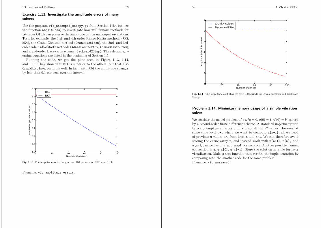
1.9 Exercises and Problems 63
Exercise 1.13: Investigate the amplitude errors of manysolvers
Use the program vib_undamped_odespy.py from Section 1.5.4 (utilizethe function amplitudes) to investigate how well famous methods for1st-order ODEs can preserve the amplitude of u in undamped oscillations.Test, for example, the 3rd- and 4th-order Runge-Kutta methods (RK3,RK4), the Crank-Nicolson method (CrankNicolson), the 2nd- and 3rd-order Adams-Bashforth methods (AdamsBashforth2, AdamsBashforth3),and a 2nd-order Backwards scheme (Backward2Step). The relevant gov-erning equations are listed in the beginning of Section 1.5.
Running the code, we get the plots seen in Figure 1.13, 1.14,and 1.15. They show that RK4 is superior to the others, but that alsoCrankNicolson performs well. In fact, with RK4 the amplitude changesby less than 0.1 per cent over the interval.
0 20 40 60 80 100Number of periods
4.8
5.0
5.2
5.4
5.6
5.8
6.0
6.2
6.4
Ampl
itude
(abs
olut
e va
lue)
RK3RK4
Fig. 1.13 The amplitude as it changes over 100 periods for RK3 and RK4.
Filename: vib_amplitude_errors.
64 1 Vibration ODEs
0 20 40 60 80 100Number of periods
1
2
3
4
5
6
7
Ampl
itude
(abs
olut
e va
lue)
CrankNicolsonBackward2Step
Fig. 1.14 The amplitude as it changes over 100 periods for Crank-Nicolson and Backward2 step.
Problem 1.14: Minimize memory usage of a simple vibrationsolver
We consider the model problem u′′+ω2u = 0, u(0) = I, u′(0) = V , solvedby a second-order finite difference scheme. A standard implementationtypically employs an array u for storing all the un values. However, atsome time level n+1 where we want to compute u[n+1], all we needof previous u values are from level n and n-1. We can therefore avoidstoring the entire array u, and instead work with u[n+1], u[n], andu[n-1], named as u, u_n, u_nmp1, for instance. Another possible namingconvention is u, u_n[0], u_n[-1]. Store the solution in a file for latervisualization. Make a test function that verifies the implementation bycomparing with the another code for the same problem.Filename: vib_memsave0.
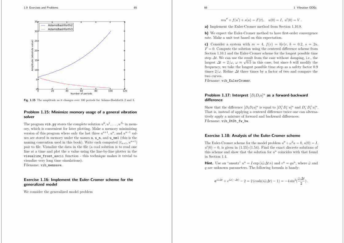
1.9 Exercises and Problems 65
0 20 40 60 80 100 120Number of periods
0
5
10
15
20
25
30
35
Ampl
itude
(abs
olut
e va
lue)
AdamsBashforth2AdamsBashforth3
Fig. 1.15 The amplitude as it changes over 100 periods for Adams-Bashforth 2 and 3.
Problem 1.15: Minimize memory usage of a general vibrationsolver
The program vib.py stores the complete solution u0, u1, . . . , uNt in mem-ory, which is convenient for later plotting. Make a memory minimizingversion of this program where only the last three un+1, un, and un−1 val-ues are stored in memory under the names u, u_n, and u_nm1 (this is thenaming convention used in this book). Write each computed (tn+1, u
n+1)pair to file. Visualize the data in the file (a cool solution is to read oneline at a time and plot the u value using the line-by-line plotter in thevisualize_front_ascii function - this technique makes it trivial tovisualize very long time simulations).Filename: vib_memsave.
Exercise 1.16: Implement the Euler-Cromer scheme for thegeneralized model
We consider the generalized model problem
66 1 Vibration ODEs
mu′′ + f(u′) + s(u) = F (t), u(0) = I, u′(0) = V .
a) Implement the Euler-Cromer method from Section 1.10.8.
b) We expect the Euler-Cromer method to have first-order convergencerate. Make a unit test based on this expectation.
c) Consider a system with m = 4, f(v) = b|v|v, b = 0.2, s = 2u,F = 0. Compute the solution using the centered difference scheme fromSection 1.10.1 and the Euler-Cromer scheme for the longest possible timestep ∆t. We can use the result from the case without damping, i.e., thelargest ∆t = 2/ω, ω ≈
√0.5 in this case, but since b will modify the
frequency, we take the longest possible time step as a safety factor 0.9times 2/ω. Refine ∆t three times by a factor of two and compare thetwo curves.Filename: vib_EulerCromer.
Problem 1.17: Interpret [DtDtu]n as a forward-backwarddifference
Show that the difference [DtDtu]n is equal to [D+t D
−t u]n and D−t D+
t u]n.That is, instead of applying a centered difference twice one can alterna-tively apply a mixture of forward and backward differences.Filename: vib_DtDt_fw_bw.
Exercise 1.18: Analysis of the Euler-Cromer scheme
The Euler-Cromer scheme for the model problem u′′+ω2u = 0, u(0) = I,u′(0) = 0, is given in (1.55)-(1.54). Find the exact discrete solutions ofthis scheme and show that the solution for un coincides with that foundin Section 1.4.
Hint. Use an “ansatz” un = I exp (iω∆t n) and vn = qun, where ω andq are unknown parameters. The following formula is handy:
eiω∆t + eiω(−∆t) − 2 = 2 (cosh(iω∆t)− 1) = −4 sin2( ω∆t2 ) .
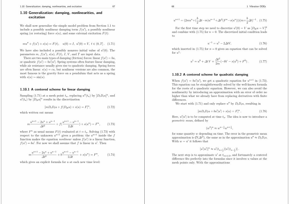
1.10 Generalization: damping, nonlinearities, and excitation 67
1.10 Generalization: damping, nonlinearities, andexcitation
We shall now generalize the simple model problem from Section 1.1 toinclude a possibly nonlinear damping term f(u′), a possibly nonlinearspring (or restoring) force s(u), and some external excitation F (t):
mu′′ + f(u′) + s(u) = F (t), u(0) = I, u′(0) = V, t ∈ (0, T ] . (1.71)
We have also included a possibly nonzero initial value of u′(0). Theparameters m, f(u′), s(u), F (t), I, V , and T are input data.
There are two main types of damping (friction) forces: linear f(u′) = bu,or quadratic f(u′) = bu′|u′|. Spring systems often feature linear damping,while air resistance usually gives rise to quadratic damping. Spring forcesare often linear: s(u) = cu, but nonlinear versions are also common, themost famous is the gravity force on a pendulum that acts as a springwith s(u) ∼ sin(u).
1.10.1 A centered scheme for linear damping
Sampling (1.71) at a mesh point tn, replacing u′′(tn) by [DtDtu]n, andu′(tn) by [D2tu]n results in the discretization
[mDtDtu+ f(D2tu) + s(u) = F ]n, (1.72)
which written out means
mun+1 − 2un + un−1
∆t2+ f(u
n+1 − un−1
2∆t ) + s(un) = F n, (1.73)
where F n as usual means F (t) evaluated at t = tn. Solving (1.73) withrespect to the unknown un+1 gives a problem: the un+1 inside the ffunction makes the equation nonlinear unless f(u′) is a linear function,f(u′) = bu′. For now we shall assume that f is linear in u′. Then
mun+1 − 2un + un−1
∆t2+ b
un+1 − un−1
2∆t + s(un) = F n, (1.74)
which gives an explicit formula for u at each new time level:
68 1 Vibration ODEs
un+1 = (2mun+( b2∆t−m)un−1+∆t2(F n−s(un)))(m+ b
2∆t)−1 . (1.75)
For the first time step we need to discretize u′(0) = V as [D2tu = V ]0and combine with (1.75) for n = 0. The discretized initial condition leadsto
u−1 = u1 − 2∆tV, (1.76)
which inserted in (1.75) for n = 0 gives an equation that can be solvedfor u1:
u1 = u0 +∆tV + ∆t2
2m (−bV − s(u0) + F 0) . (1.77)
1.10.2 A centered scheme for quadratic damping
When f(u′) = bu′|u′|, we get a quadratic equation for un+1 in (1.73).This equation can be straightforwardly solved by the well-known formulafor the roots of a quadratic equation. However, we can also avoid thenonlinearity by introducing an approximation with an error of order nohigher than what we already have from replacing derivatives with finitedifferences.
We start with (1.71) and only replace u′′ by DtDtu, resulting in
[mDtDtu+ bu′|u′|+ s(u) = F ]n . (1.78)
Here, u′|u′| is to be computed at time tn. The idea is now to introduce ageometric mean, defined by
(w2)n ≈ wn−12wn+ 1
2 ,
for some quantity w depending on time. The error in the geometric meanapproximation is O(∆t2), the same as in the approximation u′′ ≈ DtDtu.With w = u′ it follows that
[u′|u′|]n ≈ u′(tn+ 12)|u′(tn− 1
2)| .
The next step is to approximate u′ at tn±1/2, and fortunately a centereddifference fits perfectly into the formulas since it involves u values at themesh points only. With the approximations
1.10 Generalization: damping, nonlinearities, and excitation 69
u′(tn+1/2) ≈ [Dtu]n+ 12 , u′(tn−1/2) ≈ [Dtu]n− 1
2 , (1.79)
we get
[u′|u′|]n ≈ [Dtu]n+ 12 |[Dtu]n− 1
2 | = un+1 − un∆t
|un − un−1|∆t
. (1.80)
The counterpart to (1.73) is then
mun+1 − 2un + un−1
∆t2+ b
un+1 − un∆t
|un − un−1|∆t
+ s(un) = F n, (1.81)
which is linear in the unknown un+1. Therefore, we can easily solve (1.81)with respect to un+1 and achieve the explicit updating formula
un+1 =(m+ b|un − un−1|
)−1×
(2mun −mun−1 + bun|un − un−1|+∆t2(F n − s(un))
).
(1.82)
In the derivation of a special equation for the first time step we run intosome trouble: inserting (1.76) in (1.82) for n = 0 results in a complicatednonlinear equation for u1. By thinking differently about the problem wecan easily get away with the nonlinearity again. We have for n = 0 thatb[u′|u′|]0 = bV |V |. Using this value in (1.78) gives
[mDtDtu+ bV |V |+ s(u) = F ]0 . (1.83)
Writing this equation out and using (1.76) results in the special equationfor the first time step:
u1 = u0 +∆tV + ∆t2
2m(−bV |V | − s(u0) + F 0
). (1.84)
1.10.3 A forward-backward discretization of the quadraticdamping term
The previous section first proposed to discretize the quadratic dampingterm |u′|u′ using centered differences: [|D2t|D2tu]n. As this gives rise toa nonlinearity in un+1, it was instead proposed to use a geometric mean
70 1 Vibration ODEs
combined with centered differences. But there are other alternatives.To get rid of the nonlinearity in [|D2t|D2tu]n, one can think differently:apply a backward difference to |u′|, such that the term involves knownvalues, and apply a forward difference to u′ to make the term linear inthe unknown un+1. With mathematics,
[β|u′|u′]n ≈ β|[D−t u]n|[D+t u]n = β
∣∣∣∣∣un − un−1
∆t
∣∣∣∣∣un+1 − un
∆t. (1.85)
The forward and backward differences have both an error proportional to∆t so one may think the discretization above leads to a first-order scheme.However, by looking at the formulas, we realize that the forward-backwarddifferences in (1.85) result in exactly the same scheme as in (1.81) wherewe used a geometric mean and centered differences and committed errorsof size O(∆t2). Therefore, the forward-backward differences in (1.85)act in a symmetric way and actually produce a second-order accuratediscretization of the quadratic damping term.
1.10.4 Implementation
The algorithm arising from the methods in Sections 1.10.1 and 1.10.2is very similar to the undamped case in Section 1.1.2. The difference isbasically a question of different formulas for u1 and un+1. This is actuallyquite remarkable. The equation (1.71) is normally impossible to solve bypen and paper, but possible for some special choices of F , s, and f . Onthe contrary, the complexity of the nonlinear generalized model (1.71)versus the simple undamped model is not a big deal when we solve theproblem numerically!
The computational algorithm takes the form
1. u0 = I2. compute u1 from (1.77) if linear damping or (1.84) if quadratic damp-
ing3. for n = 1, 2, . . . , Nt − 1:
a. compute un+1 from (1.75) if linear damping or (1.82) if quadraticdamping
Modifying the solver function for the undamped case is fairly easy, thebig difference being many more terms and if tests on the type of damping:
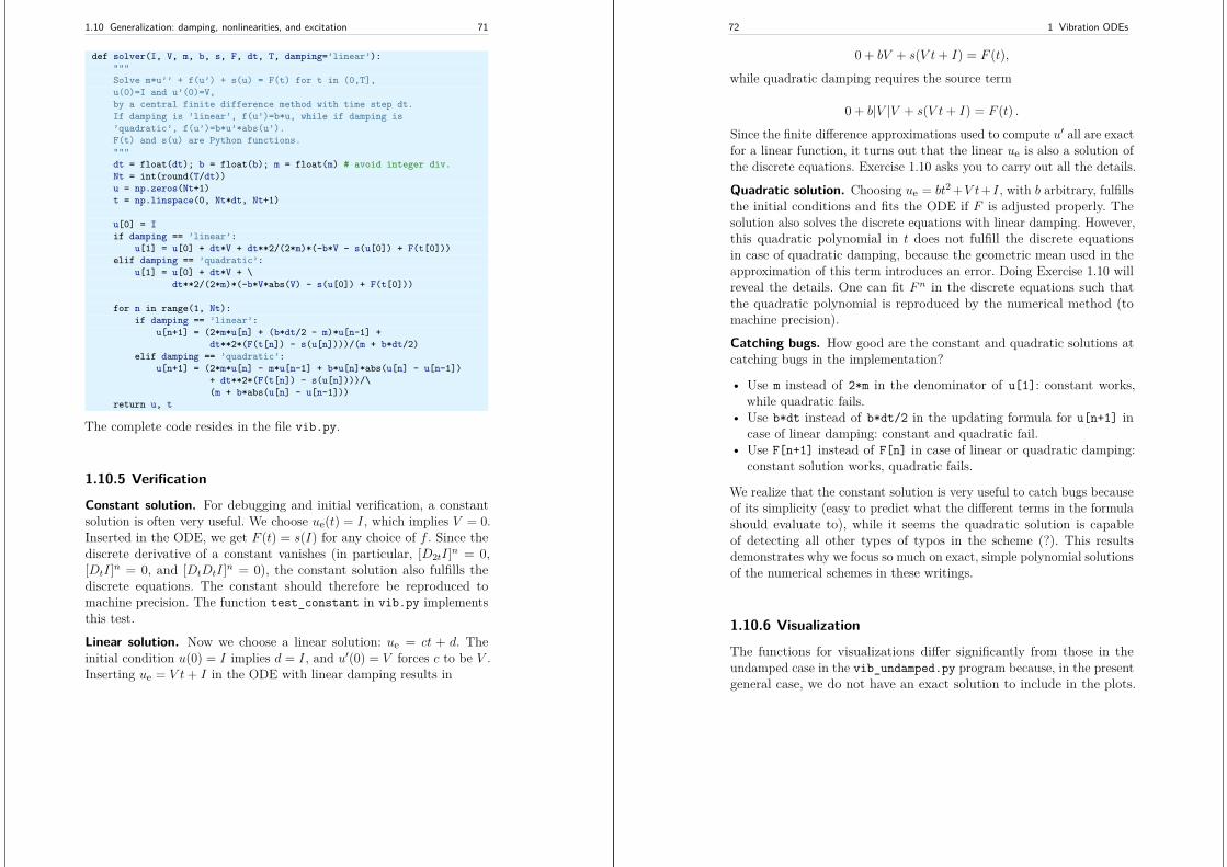
1.10 Generalization: damping, nonlinearities, and excitation 71
def solver(I, V, m, b, s, F, dt, T, damping=’linear’):"""Solve m*u’’ + f(u’) + s(u) = F(t) for t in (0,T],u(0)=I and u’(0)=V,by a central finite difference method with time step dt.If damping is ’linear’, f(u’)=b*u, while if damping is’quadratic’, f(u’)=b*u’*abs(u’).F(t) and s(u) are Python functions."""dt = float(dt); b = float(b); m = float(m) # avoid integer div.Nt = int(round(T/dt))u = np.zeros(Nt+1)t = np.linspace(0, Nt*dt, Nt+1)
u[0] = Iif damping == ’linear’:
u[1] = u[0] + dt*V + dt**2/(2*m)*(-b*V - s(u[0]) + F(t[0]))elif damping == ’quadratic’:
u[1] = u[0] + dt*V + \dt**2/(2*m)*(-b*V*abs(V) - s(u[0]) + F(t[0]))
for n in range(1, Nt):if damping == ’linear’:
u[n+1] = (2*m*u[n] + (b*dt/2 - m)*u[n-1] +dt**2*(F(t[n]) - s(u[n])))/(m + b*dt/2)
elif damping == ’quadratic’:u[n+1] = (2*m*u[n] - m*u[n-1] + b*u[n]*abs(u[n] - u[n-1])
+ dt**2*(F(t[n]) - s(u[n])))/\(m + b*abs(u[n] - u[n-1]))
return u, t
The complete code resides in the file vib.py.
1.10.5 Verification
Constant solution. For debugging and initial verification, a constantsolution is often very useful. We choose ue(t) = I, which implies V = 0.Inserted in the ODE, we get F (t) = s(I) for any choice of f . Since thediscrete derivative of a constant vanishes (in particular, [D2tI]n = 0,[DtI]n = 0, and [DtDtI]n = 0), the constant solution also fulfills thediscrete equations. The constant should therefore be reproduced tomachine precision. The function test_constant in vib.py implementsthis test.
Linear solution. Now we choose a linear solution: ue = ct + d. Theinitial condition u(0) = I implies d = I, and u′(0) = V forces c to be V .Inserting ue = V t+ I in the ODE with linear damping results in
72 1 Vibration ODEs
0 + bV + s(V t+ I) = F (t),
while quadratic damping requires the source term
0 + b|V |V + s(V t+ I) = F (t) .
Since the finite difference approximations used to compute u′ all are exactfor a linear function, it turns out that the linear ue is also a solution ofthe discrete equations. Exercise 1.10 asks you to carry out all the details.
Quadratic solution. Choosing ue = bt2 +V t+I, with b arbitrary, fulfillsthe initial conditions and fits the ODE if F is adjusted properly. Thesolution also solves the discrete equations with linear damping. However,this quadratic polynomial in t does not fulfill the discrete equationsin case of quadratic damping, because the geometric mean used in theapproximation of this term introduces an error. Doing Exercise 1.10 willreveal the details. One can fit F n in the discrete equations such thatthe quadratic polynomial is reproduced by the numerical method (tomachine precision).
Catching bugs. How good are the constant and quadratic solutions atcatching bugs in the implementation?
• Use m instead of 2*m in the denominator of u[1]: constant works,while quadratic fails.
• Use b*dt instead of b*dt/2 in the updating formula for u[n+1] incase of linear damping: constant and quadratic fail.
• Use F[n+1] instead of F[n] in case of linear or quadratic damping:constant solution works, quadratic fails.
We realize that the constant solution is very useful to catch bugs becauseof its simplicity (easy to predict what the different terms in the formulashould evaluate to), while it seems the quadratic solution is capableof detecting all other types of typos in the scheme (?). This resultsdemonstrates why we focus so much on exact, simple polynomial solutionsof the numerical schemes in these writings.
1.10.6 Visualization
The functions for visualizations differ significantly from those in theundamped case in the vib_undamped.py program because, in the presentgeneral case, we do not have an exact solution to include in the plots.
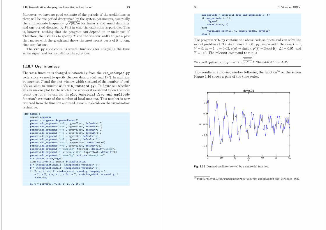
1.10 Generalization: damping, nonlinearities, and excitation 73
Moreover, we have no good estimate of the periods of the oscillations asthere will be one period determined by the system parameters, essentiallythe approximate frequency
√s′(0)/m for linear s and small damping,
and one period dictated by F (t) in case the excitation is periodic. Thisis, however, nothing that the program can depend on or make use of.Therefore, the user has to specify T and the window width to get a plotthat moves with the graph and shows the most recent parts of it in longtime simulations.
The vib.py code contains several functions for analyzing the timeseries signal and for visualizing the solutions.
1.10.7 User interfaceThe main function is changed substantially from the vib_undamped.pycode, since we need to specify the new data c, s(u), and F (t). In addition,we must set T and the plot window width (instead of the number of peri-ods we want to simulate as in vib_undamped.py). To figure out whetherwe can use one plot for the whole time series or if we should follow the mostrecent part of u, we can use the plot_empricial_freq_and_amplitudefunction’s estimate of the number of local maxima. This number is nowreturned from the function and used in main to decide on the visualizationtechnique.
def main():import argparseparser = argparse.ArgumentParser()parser.add_argument(’--I’, type=float, default=1.0)parser.add_argument(’--V’, type=float, default=0.0)parser.add_argument(’--m’, type=float, default=1.0)parser.add_argument(’--c’, type=float, default=0.0)parser.add_argument(’--s’, type=str, default=’u’)parser.add_argument(’--F’, type=str, default=’0’)parser.add_argument(’--dt’, type=float, default=0.05)parser.add_argument(’--T’, type=float, default=140)parser.add_argument(’--damping’, type=str, default=’linear’)parser.add_argument(’--window_width’, type=float, default=30)parser.add_argument(’--savefig’, action=’store_true’)a = parser.parse_args()from scitools.std import StringFunctions = StringFunction(a.s, independent_variable=’u’)F = StringFunction(a.F, independent_variable=’t’)I, V, m, c, dt, T, window_width, savefig, damping = \
a.I, a.V, a.m, a.c, a.dt, a.T, a.window_width, a.savefig, \a.damping
u, t = solver(I, V, m, c, s, F, dt, T)
74 1 Vibration ODEs
num_periods = empirical_freq_and_amplitude(u, t)if num_periods <= 15:
figure()visualize(u, t)
else:visualize_front(u, t, window_width, savefig)
show()
The program vib.py contains the above code snippets and can solve themodel problem (1.71). As a demo of vib.py, we consider the case I = 1,V = 0, m = 1, c = 0.03, s(u) = sin(u), F (t) = 3 cos(4t), ∆t = 0.05, andT = 140. The relevant command to run is
Terminal
Terminal> python vib.py --s ’sin(u)’ --F ’3*cos(4*t)’ --c 0.03
This results in a moving window following the function16 on the screen.Figure 1.16 shows a part of the time series.
0 10 20 30 40 50 60t
1.0
0.5
0.0
0.5
1.0
u
dt=0.05
Fig. 1.16 Damped oscillator excited by a sinusoidal function.
16 http://tinyurl.com/pu5uyfn/pub/mov-vib/vib_generalized_dt0.05/index.html
1.10 Generalization: damping, nonlinearities, and excitation 75
1.10.8 The Euler-Cromer scheme for the generalized model
The ideas of the Euler-Cromer method from Section 1.7 carry over to thegeneralized model. We write (1.71) as two equations for u and v = u′.The first equation is taken as the one with v′ on the left-hand side:
v′ = 1m
(F (t)− s(u)− f(v)), (1.86)
u′ = v . (1.87)
The idea is to step (1.86) forward using a standard Forward Euler method,while we update u from (1.87) with a Backward Euler method, utilizingthe recent, computed vn+1 value. In detail,
vn+1 − vn∆t
= 1m
(F (tn)− s(un)− f(vn)), (1.88)
un+1 − un∆t
= vn+1, (1.89)
resulting in the explicit scheme
vn+1 = vn +∆t1m
(F (tn)− s(un)− f(vn)), (1.90)
un+1 = un +∆t vn+1 . (1.91)
We immediately note one very favorable feature of this scheme: all thenonlinearities in s(u) and f(v) are evaluated at a previous time level.This makes the Euler-Cromer method easier to apply and hence muchmore convenient than the centered scheme for the second-order ODE(1.71).
The initial conditions are trivially set as
v0 = V, (1.92)u0 = I . (1.93)
76 1 Vibration ODEs
1.10.9 The Störmer-Verlet algorithm for the generalizedmodel
We can easily apply the ideas from Section 1.7.4 to extend that methodto the generalized model
v′ = 1m
(F (t)− s(u)− f(v)),
u′ = v .
However, since the scheme is essentially centered differences for the ODEsystem on a staggered mesh, we do not go into detail here, but refer toSection 1.10.10.
1.10.10 A staggered Euler-Cromer scheme for a generalizedmodel
The more general model for vibration problems,
mu′′ + f(u′) + s(u) = F (t), u(0) = I, u′(0) = V, t ∈ (0, T ], (1.94)
can be rewritten as a first-order ODE system
v′ = m−1 (F (t)− f(v)− s(u)) , (1.95)u′ = v . (1.96)
It is natural to introduce a staggered mesh (see Section 1.8.1) andseek u at mesh points tn (the numerical value is denoted by un) and vbetween mesh points at tn+1/2 (the numerical value is denoted by vn+ 1
2 ).A centered difference approximation to (1.96)-(1.95) can then be writtenin operator notation as
[Dtv = m−1 (F (t)− f(v)− s(u))]n, (1.97)[Dtu = v]n+ 1
2 . (1.98)
Written out,
1.10 Generalization: damping, nonlinearities, and excitation 77
vn+ 12 − vn− 1
2
∆t= m−1 (F n − f(vn)− s(un)) , (1.99)
un − un−1
∆t= vn+ 1
2 . (1.100)
With linear damping, f(v) = bv, we can use an arithmetic mean forf(vn): f(vn) ≈= 1
2(f(vn− 12 ) + f(vn+ 1
2 )). The system (1.99)-(1.100) canthen be solved with respect to the unknowns un and vn+ 1
2 :
vn+ 12 =
(1 + b
2m∆t
)−1 (vn−
12 +∆tm−1
(F n − 1
2f(vn− 12 )− s(un)
)),
(1.101)un = un−1 +∆tvn−
12 . (1.102)
In case of quadratic damping, f(v) = b|v|v, we can use a geometricmean: f(vn) ≈ b|vn− 1
2 |vn+ 12 . Inserting this approximation in (1.99)-
(1.100) and solving for the unknowns un and vn+ 12 results in
vn+ 12 = (1 + b
m|vn− 1
2 |∆t)−1(vn−
12 +∆tm−1 (F n − s(un))
), (1.103)
un = un−1 +∆tvn−12 . (1.104)
The initial conditions are derived at the end of Section 1.8.1:
u0 = I, (1.105)
v12 = V − 1
2∆tω2I . (1.106)
1.10.11 The PEFRL 4th-order accurate algorithmA variant of the Euler-Cromer type of algorithm, which provides anerror O(∆t4) if f(v) = 0, is called PEFRL [14]. This algorithm is verywell suited for integrating dynamic systems (especially those withoutdamping) over very long time periods. Define
g(u, v) = 1m
(F (t)− s(u)− f(v)) .
The algorithm is explicit and features these simple steps:
78 1 Vibration ODEs
un+1,1 = un + ξ∆tvn, (1.107)
vn+1,1 = vn + 12(1− 2λ)∆tg(un+1,1, vn), (1.108)
un+1,2 = un+1,1 + χ∆tvn+1,1, (1.109)vn+1,2 = vn+1,1 + λ∆tg(un+1,2, vn+1,1), (1.110)un+1,3 = un+1,2 + (1− 2(χ+ ξ))∆tvn+1,2, (1.111)vn+1,3 = vn+1,2 + λ∆tg(un+1,3, vn+1,2), (1.112)un+1,4 = un+1,3 + χ∆tvn+1,3, (1.113)
vn+1 = vn+1,3 + 12(1− 2λ)∆tg(un+1,4, vn+1,3), (1.114)
un+1 = un+1,4 + ξ∆tvn+1 (1.115)
The parameters ξ, λ, and ξ have the values
ξ = 0.1786178958448091, (1.116)λ = −0.2123418310626054, (1.117)χ = −0.06626458266981849 (1.118)
1.11 Exercises and Problems
Exercise 1.19: Implement the solver via classes
Reimplement the vib.py program using a class Problem to hold all thephysical parameters of the problem, a class Solver to hold the numericalparameters and compute the solution, and a class Visualizer to displaythe solution.
Hint. Use the ideas and examples from Section ?? and ?? in [9]. Morespecifically, make a superclass Problem for holding the scalar physicalparameters of a problem and let subclasses implement the s(u) and F (t)functions as methods. Try to call up as much existing functionality invib.py as possible.Filename: vib_class.
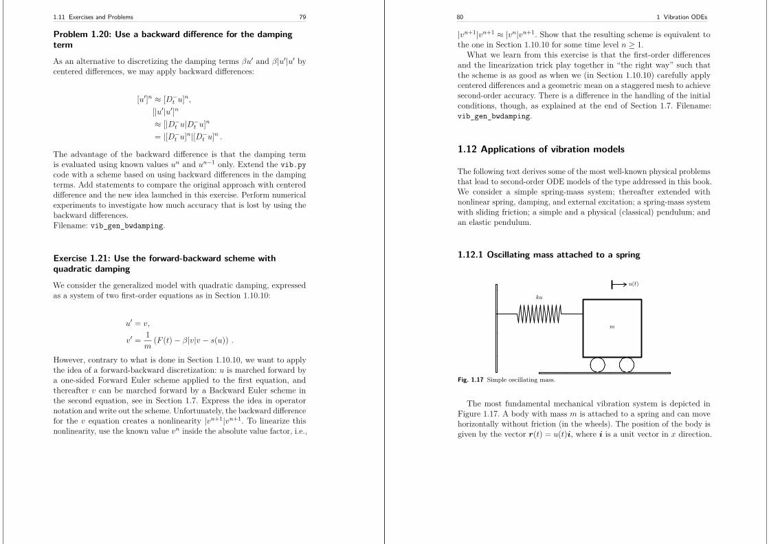
1.11 Exercises and Problems 79
Problem 1.20: Use a backward difference for the dampingterm
As an alternative to discretizing the damping terms βu′ and β|u′|u′ bycentered differences, we may apply backward differences:
[u′]n ≈ [D−t u]n,[|u′|u′]n≈ [|D−t u|D−t u]n
= |[D−t u]n|[D−t u]n .
The advantage of the backward difference is that the damping termis evaluated using known values un and un−1 only. Extend the vib.pycode with a scheme based on using backward differences in the dampingterms. Add statements to compare the original approach with centereddifference and the new idea launched in this exercise. Perform numericalexperiments to investigate how much accuracy that is lost by using thebackward differences.Filename: vib_gen_bwdamping.
Exercise 1.21: Use the forward-backward scheme withquadratic damping
We consider the generalized model with quadratic damping, expressedas a system of two first-order equations as in Section 1.10.10:
u′ = v,
v′ = 1m
(F (t)− β|v|v − s(u)) .
However, contrary to what is done in Section 1.10.10, we want to applythe idea of a forward-backward discretization: u is marched forward bya one-sided Forward Euler scheme applied to the first equation, andthereafter v can be marched forward by a Backward Euler scheme inthe second equation, see in Section 1.7. Express the idea in operatornotation and write out the scheme. Unfortunately, the backward differencefor the v equation creates a nonlinearity |vn+1|vn+1. To linearize thisnonlinearity, use the known value vn inside the absolute value factor, i.e.,
80 1 Vibration ODEs
|vn+1|vn+1 ≈ |vn|vn+1. Show that the resulting scheme is equivalent tothe one in Section 1.10.10 for some time level n ≥ 1.
What we learn from this exercise is that the first-order differencesand the linearization trick play together in “the right way” such thatthe scheme is as good as when we (in Section 1.10.10) carefully applycentered differences and a geometric mean on a staggered mesh to achievesecond-order accuracy. There is a difference in the handling of the initialconditions, though, as explained at the end of Section 1.7. Filename:vib_gen_bwdamping.
1.12 Applications of vibration models
The following text derives some of the most well-known physical problemsthat lead to second-order ODE models of the type addressed in this book.We consider a simple spring-mass system; thereafter extended withnonlinear spring, damping, and external excitation; a spring-mass systemwith sliding friction; a simple and a physical (classical) pendulum; andan elastic pendulum.
1.12.1 Oscillating mass attached to a spring
ku
u(t)
m
Fig. 1.17 Simple oscillating mass.
The most fundamental mechanical vibration system is depicted inFigure 1.17. A body with mass m is attached to a spring and can movehorizontally without friction (in the wheels). The position of the body isgiven by the vector r(t) = u(t)i, where i is a unit vector in x direction.
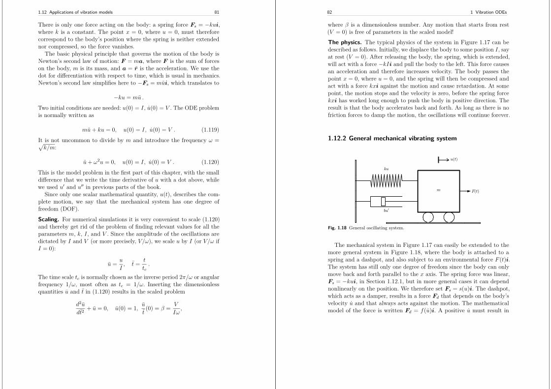
1.12 Applications of vibration models 81
There is only one force acting on the body: a spring force Fs = −kui,where k is a constant. The point x = 0, where u = 0, must thereforecorrespond to the body’s position where the spring is neither extendednor compressed, so the force vanishes.
The basic physical principle that governs the motion of the body isNewton’s second law of motion: F = ma, where F is the sum of forceson the body, m is its mass, and a = r is the acceleration. We use thedot for differentiation with respect to time, which is usual in mechanics.Newton’s second law simplifies here to −Fs = mui, which translates to
−ku = mu .
Two initial conditions are needed: u(0) = I, u(0) = V . The ODE problemis normally written as
mu+ ku = 0, u(0) = I, u(0) = V . (1.119)
It is not uncommon to divide by m and introduce the frequency ω =√k/m:
u+ ω2u = 0, u(0) = I, u(0) = V . (1.120)
This is the model problem in the first part of this chapter, with the smalldifference that we write the time derivative of u with a dot above, whilewe used u′ and u′′ in previous parts of the book.
Since only one scalar mathematical quantity, u(t), describes the com-plete motion, we say that the mechanical system has one degree offreedom (DOF).
Scaling. For numerical simulations it is very convenient to scale (1.120)and thereby get rid of the problem of finding relevant values for all theparameters m, k, I, and V . Since the amplitude of the oscillations aredictated by I and V (or more precisely, V/ω), we scale u by I (or V/ω ifI = 0):
u = u
I, t = t
tc.
The time scale tc is normally chosen as the inverse period 2π/ω or angularfrequency 1/ω, most often as tc = 1/ω. Inserting the dimensionlessquantities u and t in (1.120) results in the scaled problem
d2u
dt2+ u = 0, u(0) = 1, u
t(0) = β = V
Iω,
82 1 Vibration ODEs
where β is a dimensionless number. Any motion that starts from rest(V = 0) is free of parameters in the scaled model!The physics. The typical physics of the system in Figure 1.17 can bedescribed as follows. Initially, we displace the body to some position I, sayat rest (V = 0). After releasing the body, the spring, which is extended,will act with a force −kIi and pull the body to the left. This force causesan acceleration and therefore increases velocity. The body passes thepoint x = 0, where u = 0, and the spring will then be compressed andact with a force kxi against the motion and cause retardation. At somepoint, the motion stops and the velocity is zero, before the spring forcekxi has worked long enough to push the body in positive direction. Theresult is that the body accelerates back and forth. As long as there is nofriction forces to damp the motion, the oscillations will continue forever.
1.12.2 General mechanical vibrating system
m F(t)
u(t)
bu′
ku
Fig. 1.18 General oscillating system.
The mechanical system in Figure 1.17 can easily be extended to themore general system in Figure 1.18, where the body is attached to aspring and a dashpot, and also subject to an environmental force F (t)i.The system has still only one degree of freedom since the body can onlymove back and forth parallel to the x axis. The spring force was linear,Fs = −kui, in Section 1.12.1, but in more general cases it can dependnonlinearly on the position. We therefore set Fs = s(u)i. The dashpot,which acts as a damper, results in a force Fd that depends on the body’svelocity u and that always acts against the motion. The mathematicalmodel of the force is written Fd = f(u)i. A positive u must result in
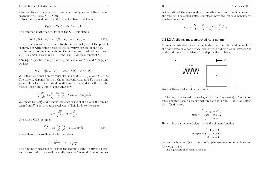
1.12 Applications of vibration models 83
a force acting in the positive x direction. Finally, we have the externalenvironmental force Fe = F (t)i.
Newton’s second law of motion now involves three forces:
F (t)i+ f(u)i− s(u)i = mui .
The common mathematical form of the ODE problem is
mu+ f(u) + s(u) = F (t), u(0) = I, u(0) = V . (1.121)
This is the generalized problem treated in the last part of the presentchapter, but with prime denoting the derivative instead of the dot.
The most common models for the spring and dashpot are linear:f(u) = bu with a constant b ≥ 0, and s(u) = ku for a constant k.
Scaling. A specific scaling requires specific choices of f , s, and F . Supposewe have
f(u) = b|u|u, s(u) = ku, F (t) = A sin(φt) .
We introduce dimensionless variables as usual, u = u/uc and t = t/tc.The scale uc depends both on the initial conditions and F , but as timegrows, the effect of the initial conditions die out and F will drive themotion. Inserting u and t in the ODE gives
muct2c
d2u
dt2+ b
u2c
t2c
∣∣∣∣du
dt
∣∣∣∣du
dt+ kucu = A sin(φtct) .
We divide by uc/t2c and demand the coefficients of the u and the forcingterm from F (t) to have unit coefficients. This leads to the scales
tc =√m
k, uc = A
k.
The scaled ODE becomes
d2u
dt2+ 2β
∣∣∣∣du
dt
∣∣∣∣du
dt+ u = sin(γt), (1.122)
where there are two dimensionless numbers:
β = Ab
2mk, γ = φ
√m
k.
The β number measures the size of the damping term (relative to unity)and is assumed to be small, basically because b is small. The φ number
84 1 Vibration ODEs
is the ratio of the time scale of free vibrations and the time scale ofthe forcing. The scaled initial conditions have two other dimensionlessnumbers as values:
u(0) = Ik
A,
du
dt= tcucV = V
A
√mk .
1.12.3 A sliding mass attached to a springConsider a variant of the oscillating body in Section 1.12.1 and Figure 1.17:the body rests on a flat surface, and there is sliding friction between thebody and the surface. Figure 1.19 depicts the problem.
s(u)
u(t)
m
Fig. 1.19 Sketch of a body sliding on a surface.
The body is attached to a spring with spring force −s(u)i. The frictionforce is proportional to the normal force on the surface, −mgj, and givenby −f(u)i, where
f(u) =
−µmg, u < 0,µmg, u > 0,0, u = 0
Here, µ is a friction coefficient. With the signum function
sign(x) =
−1, x < 0,1, x > 0,0, x = 0
we can simply write f(u) = µmg sign(u) (the sign function is implementedby numpy.sign).
The equation of motion becomes
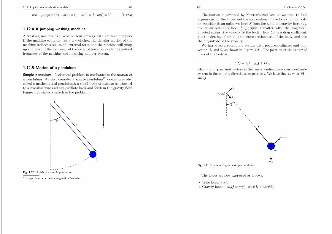
1.12 Applications of vibration models 85
mu+ µmgsign(u) + s(u) = 0, u(0) = I, u(0) = V . (1.123)
1.12.4 A jumping washing machine
A washing machine is placed on four springs with efficient dampers.If the machine contains just a few clothes, the circular motion of themachine induces a sinusoidal external force and the machine will jumpup and down if the frequency of the external force is close to the naturalfrequency of the machine and its spring-damper system.
1.12.5 Motion of a pendulum
Simple pendulum. A classical problem in mechanics is the motion ofa pendulum. We first consider a simple pendulum17 (sometimes alsocalled a mathematical pendulum): a small body of mass m is attachedto a massless wire and can oscillate back and forth in the gravity field.Figure 1.20 shows a sketch of the problem.
g
m
L
θ
Fig. 1.20 Sketch of a simple pendulum.17 https://en.wikipedia.org/wiki/Pendulum
86 1 Vibration ODEs
The motion is governed by Newton’s 2nd law, so we need to findexpressions for the forces and the acceleration. Three forces on the bodyare considered: an unknown force S from the wire, the gravity force mg,and an air resistance force, 1
2CD%A|v|v, hereafter called the drag force,directed against the velocity of the body. Here, CD is a drag coefficient,% is the density of air, A is the cross section area of the body, and v isthe magnitude of the velocity.
We introduce a coordinate system with polar coordinates and unitvectors ir and iθ as shown in Figure 1.21. The position of the center ofmass of the body is
r(t) = x0i+ y0j + Lir,
where i and j are unit vectors in the corresponding Cartesian coordinatesystem in the x and y directions, respectively. We have that ir = cos θi+sin θj.
(x0 ,y0 )
mg
iθ
m
ir
∼|v|v
S
θ
Fig. 1.21 Forces acting on a simple pendulum.
The forces are now expressed as follows.
• Wire force: −Sir• Gravity force: −mgj = mg(− sin θ iθ + cos θ ir)
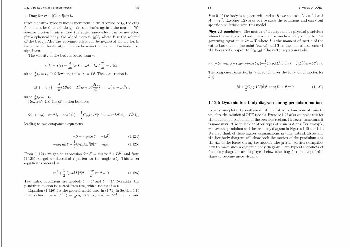
1.12 Applications of vibration models 87
• Drag force: −12CD%A|v|v iθ
Since a positive velocity means movement in the direction of iθ, the dragforce must be directed along −iθ so it works against the motion. Weassume motion in air so that the added mass effect can be neglected(for a spherical body, the added mass is 1
2%V , where V is the volumeof the body). Also the buoyancy effect can be neglected for motion inthe air when the density difference between the fluid and the body is sosignificant.
The velocity of the body is found from r:
v(t) = r(t) = d
dθ(x0i+ y0j + Lir)
dθ
dt= Lθiθ,
since ddθ ir = iθ. It follows that v = |v| = Lθ. The acceleration is
a(t) = v(r) = d
dt(Lθiθ) = Lθiθ + Lθ
diθdθθ == Lθiθ − Lθ2ir,
since ddθ iθ = −ir.
Newton’s 2nd law of motion becomes
−Sir +mg(− sin θ iθ + cos θ ir)−12CD%AL
2|θ|θ iθ = mLθθ iθ − Lθ2ir,
leading to two component equations
−S +mg cos θ = −Lθ2, (1.124)
−mg sin θ − 12CD%AL
2|θ|θ = mLθ . (1.125)
From (1.124) we get an expression for S = mg cos θ + Lθ2, and from(1.125) we get a differential equation for the angle θ(t). This latterequation is ordered as
mθ + 12CD%AL|θ|θ + mg
Lsin θ = 0 . (1.126)
Two initial conditions are needed: θ = Θ and θ = Ω. Normally, thependulum motion is started from rest, which means Ω = 0.
Equation (1.126) fits the general model used in (1.71) in Section 1.10if we define u = θ, f(u′) = 1
2CD%AL|u|u, s(u) = L−1mg sin u, and
88 1 Vibration ODEs
F = 0. If the body is a sphere with radius R, we can take CD = 0.4 andA = πR2. Exercise 1.25 asks you to scale the equations and carry outspecific simulations with this model.
Physical pendulum. The motion of a compound or physical pendulumwhere the wire is a rod with mass, can be modeled very similarly. Thegoverning equation is Ia = T where I is the moment of inertia of theentire body about the point (x0, y0), and T is the sum of moments ofthe forces with respect to (x0, y0). The vector equation reads
r×(−Sir+mg(− sin θiθ+cos θir)−12CD%AL
2|θ|θiθ) = I(Lθθiθ−Lθ2ir) .
The component equation in iθ direction gives the equation of motion forθ(t):
Iθ + 12CD%AL
3|θ|θ +mgL sin θ = 0 . (1.127)
1.12.6 Dynamic free body diagram during pendulum motion
Usually one plots the mathematical quantities as functions of time tovisualize the solution of ODE models. Exercise 1.25 asks you to do this forthe motion of a pendulum in the previous section. However, sometimes itis more instructive to look at other types of visualizations. For example,we have the pendulum and the free body diagram in Figures 1.20 and 1.21.We may think of these figures as animations in time instead. Especiallythe free body diagram will show both the motion of the pendulum andthe size of the forces during the motion. The present section exemplifieshow to make such a dynamic body diagram. Two typical snapshots offree body diagrams are displayed below (the drag force is magnified 5times to become more visual!).
1.12 Applications of vibration models 89
Dynamic physical sketches, coupled to the numerical solution of differ-ential equations, requires a program to produce a sketch for the situationat each time level. Pysketcher18 is such a tool. In fact (and not surprising!)Figures 1.20 and 1.21 were drawn using Pysketcher. The details of thedrawings are explained in the Pysketcher tutorial19. Here, we outline howthis type of sketch can be used to create an animated free body diagramduring the motion of a pendulum.
Pysketcher is actually a layer of useful abstractions on top of standardplotting packages. This means that we in fact apply Matplotlib to makethe animated free body diagram, but instead of dealing with a wealth ofdetailed Matplotlib commands, we can express the drawing in terms ofmore high-level objects, e.g., objects for the wire, angle θ, body with massm, arrows for forces, etc. When the position of these objects are giventhrough variables, we can just couple those variables to the dynamicsolution of our ODE and thereby make a unique drawing for each θ valuein a simulation.
Writing the solver. Let us start with the most familiar part of thecurrent problem: writing the solver function. We use Odespy for thispurpose. We also work with dimensionless equations. Since θ can beviewed as dimensionless, we only need to introduce a dimensionless time,here taken as t = t/
√L/g. The resulting dimensionless mathematical
model for θ, the dimensionless angular velocity ω, the dimensionless wireforce S, and the dimensionless drag force D is then
18 https://github.com/hplgit/pysketcher19 http://hplgit.github.io/pysketcher/doc/web/index.html
90 1 Vibration ODEs
dω
dt= −α|ω|ω − sin θ, (1.128)
dθ
dt= ω, (1.129)
S = ω2 + cos θ, (1.130)D = −α|ω|ω, (1.131)
with
α = CD%πR2L
2m .
as a dimensionless parameter expressing the ratio of the drag force andthe gravity force. The dimensionless ω is made non-dimensional by thetime, so ω
√L/g is the corresponding angular frequency with dimensions.
A suitable function for computing (1.128)-(1.131) is listed below.
def simulate(alpha, Theta, dt, T):import odespy
def f(u, t, alpha):omega, theta = ureturn [-alpha*omega*abs(omega) - sin(theta),
omega]
import numpy as npNt = int(round(T/float(dt)))t = np.linspace(0, Nt*dt, Nt+1)solver = odespy.RK4(f, f_args=[alpha])solver.set_initial_condition([0, Theta])u, t = solver.solve(
t, terminate=lambda u, t, n: abs(u[n,1]) < 1E-3)omega = u[:,0]theta = u[:,1]S = omega**2 + np.cos(theta)drag = -alpha*np.abs(omega)*omegareturn t, theta, omega, S, drag
Drawing the free body diagram. The sketch function below appliesPysketcher objects to build a diagram like that in Figure 1.21, exceptthat we have removed the rotation point (x0, y0) and the unit vectorsin polar coordinates as these objects are not important for an animatedfree body diagram.
import systry:
from pysketcher import *except ImportError:
1.12 Applications of vibration models 91
print ’Pysketcher must be installed from’print ’https://github.com/hplgit/pysketcher’sys.exit(1)
# Overall dimensions of sketchH = 15.W = 17.
drawing_tool.set_coordinate_system(xmin=0, xmax=W, ymin=0, ymax=H,axis=False)
def sketch(theta, S, mg, drag, t, time_level):"""Draw pendulum sketch with body forces at a time levelcorresponding to time t. The drag force is indrag[time_level], the force in the wire is S[time_level],the angle is theta[time_level]."""import matha = math.degrees(theta[time_level]) # angle in degreesL = 0.4*H # Length of pendulumP = (W/2, 0.8*H) # Fixed rotation point
mass_pt = path.geometric_features()[’end’]rod = Line(P, mass_pt)
mass = Circle(center=mass_pt, radius=L/20.)mass.set_filled_curves(color=’blue’)rod_vec = rod.geometric_features()[’end’] - \
rod.geometric_features()[’start’]unit_rod_vec = unit_vec(rod_vec)mass_symbol = Text(’$m$’, mass_pt + L/10*unit_rod_vec)
rod_start = rod.geometric_features()[’start’] # Point Pvertical = Line(rod_start, rod_start + point(0,-L/3))
def set_dashed_thin_blackline(*objects):"""Set linestyle of objects to dashed, black, width=1."""for obj in objects:
obj.set_linestyle(’dashed’)obj.set_linecolor(’black’)obj.set_linewidth(1)
set_dashed_thin_blackline(vertical)set_dashed_thin_blackline(rod)angle = Arc_wText(r’$\theta$’, rod_start, L/6, -90, a,
text_spacing=1/30.)
magnitude = 1.2*L/2 # length of a unit force in figureforce = mg[time_level] # constant (scaled eq: about 1)force *= magnitudemg_force = Force(mass_pt, mass_pt + force*point(0,-1),
’’, text_pos=’end’)
92 1 Vibration ODEs
force = S[time_level]force *= magnituderod_force = Force(mass_pt, mass_pt - force*unit_vec(rod_vec),
’’, text_pos=’end’,text_spacing=(0.03, 0.01))
force = drag[time_level]force *= magnitudeair_force = Force(mass_pt, mass_pt -
force*unit_vec((rod_vec[1], -rod_vec[0])),’’, text_pos=’end’,text_spacing=(0.04,0.005))
body_diagram = Composition(’mg’: mg_force, ’S’: rod_force, ’air’: air_force,’rod’: rod, ’body’: mass’vertical’: vertical, ’theta’: angle,)
body_diagram.draw(verbose=0)drawing_tool.savefig(’tmp_%04d.png’ % time_level, crop=False)# (No cropping: otherwise movies will be very strange!)
Making the animated free body diagram. It now remains to couplethe simulate and sketch functions. We first run simulate:
from math import pi, radians, degreesimport numpy as npalpha = 0.4period = 2*pi # Use small theta approximationT = 12*period # Simulate for 12 periodsdt = period/40 # 40 time steps per perioda = 70 # Initial amplitude in degreesTheta = radians(a)
t, theta, omega, S, drag = simulate(alpha, Theta, dt, T)
The next step is to run through the time levels in the simulation andmake a sketch at each level:
for time_level, t_ in enumerate(t):sketch(theta, S, mg, drag, t_, time_level)
The individual sketches are (by the sketch function) saved in files withnames tmp_%04d.png. These can be combined to videos using (e.g.)ffmpeg. A complete function animate for running the simulation andcreating video files is listed below.
def animate():# Clean up old plot filesimport os, globfor filename in glob.glob(’tmp_*.png’) + glob.glob(’movie.*’):
os.remove(filename)# Solve problem
1.12 Applications of vibration models 93
from math import pi, radians, degreesimport numpy as npalpha = 0.4period = 2*pi # Use small theta approximationT = 12*period # Simulate for 12 periodsdt = period/40 # 40 time steps per perioda = 70 # Initial amplitude in degreesTheta = radians(a)
t, theta, omega, S, drag = simulate(alpha, Theta, dt, T)
# Visualize drag force 5 times as largedrag *= 5mg = np.ones(S.size) # Gravity force (needed in sketch)
# Draw animationimport timefor time_level, t_ in enumerate(t):
sketch(theta, S, mg, drag, t_, time_level)time.sleep(0.2) # Pause between each frame on the screen
# Make videosprog = ’ffmpeg’filename = ’tmp_%04d.png’fps = 6codecs = ’flv’: ’flv’, ’mp4’: ’libx264’,
’webm’: ’libvpx’, ’ogg’: ’libtheora’for ext in codecs:
lib = codecs[ext]cmd = ’%(prog)s -i %(filename)s -r %(fps)s ’ % vars()cmd += ’-vcodec %(lib)s movie.%(ext)s’ % vars()print(cmd)os.system(cmd)
1.12.7 Motion of an elastic pendulum
Consider a pendulum as in Figure 1.20, but this time the wire is elastic.The length of the wire when it is not stretched is L0, while L(t) is thestretched length at time t during the motion.
Stretching the elastic wire a distance ∆L gives rise to a spring forcek∆L in the opposite direction of the stretching. Let n be a unit normalvector along the wire from the point r0 = (x0, y0) and in the direction ofiθ, see Figure 1.21 for definition of (x0, y0) and iθ. Obviously, we haven = iθ, but in this modeling of an elastic pendulum we do not need polarcoordinates. Instead, it is more straightforward to develop the equationin Cartesian coordinates.
A mathematical expression for n is
94 1 Vibration ODEs
n = r − r0L(t) ,
where L(t) = ||r − r0|| is the current length of the elastic wire. Theposition vector r in Cartesian coordinates reads r(t) = x(t)i + y(t)j,where i and j are unit vectors in the x and y directions, respectively. Itis convenient to introduce the Cartesian components nx and ny of thenormal vector:
n = r − r0L(t) = x(t)− x0
L(t) i+ y(t)− y0L(t) j = nxi+ nyj .
The stretch ∆L in the wire is
∆t = L(t)− L0 .
The force in the wire is then −Sn = −k∆Ln.The other forces are the gravity and the air resistance, just as in
Figure 1.21. For motion in air we can neglect the added mass andbuoyancy effects. The main difference is that we have a model for Sin terms of the motion (as soon as we have expressed ∆L by r). Forsimplicity, we drop the air resistance term (but Exercise 1.27 asks you toinclude it).
Newton’s second law of motion applied to the body now results in
mr = −k(L− L0)n−mgj (1.132)
The two components of (1.132) are
x = − km
(L− L0)nx, (1.133)
(1.134)
y = − km
(L− L0)ny − g . (1.135)
Remarks about an elastic vs a non-elastic pendulum. Note that thederivation of the ODEs for an elastic pendulum is more straightforwardthan for a classical, non-elastic pendulum, since we avoid the details withpolar coordinates, but instead work with Newton’s second law directly inCartesian coordinates. The reason why we can do this is that the elasticpendulum undergoes a general two-dimensional motion where all theforces are known or expressed as functions of x(t) and y(t), such that
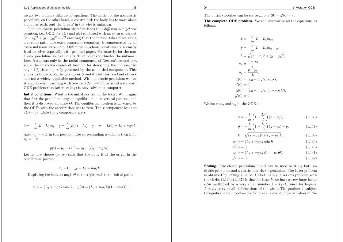
1.12 Applications of vibration models 95
we get two ordinary differential equations. The motion of the non-elasticpendulum, on the other hand, is constrained: the body has to move alonga circular path, and the force S in the wire is unknown.
The non-elastic pendulum therefore leads to a differential-algebraicequation, i.e., ODEs for x(t) and y(t) combined with an extra constraint(x− x0)2 + (y − y0)2 = L2 ensuring that the motion takes place alonga circular path. The extra constraint (equation) is compensated by anextra unknown force −Sn. Differential-algebraic equations are normallyhard to solve, especially with pen and paper. Fortunately, for the non-elastic pendulum we can do a trick: in polar coordinates the unknownforce S appears only in the radial component of Newton’s second law,while the unknown degree of freedom for describing the motion, theangle θ(t), is completely governed by the asimuthal component. Thisallows us to decouple the unknowns S and θ. But this is a kind of trickand not a widely applicable method. With an elastic pendulum we usestraightforward reasoning with Newton’s 2nd law and arrive at a standardODE problem that (after scaling) is easy solve on a computer.
Initial conditions. What is the initial position of the body? We imaginethat first the pendulum hangs in equilibrium in its vertical position, andthen it is displaced an angle Θ. The equilibrium position is governed bythe ODEs with the accelerations set to zero. The x component leads tox(t) = x0, while the y component gives
0 = − km
(L−L0)ny − g = k
m(L(0)−L0)− g ⇒ L(0) = L0 +mg/k,
since ny = −11 in this position. The corresponding y value is then fromny = −1:
y(t) = y0 − L(0) = y0 − (L0 +mg/k) .
Let us now choose (x0, y0) such that the body is at the origin in theequilibrium position:
x0 = 0, y0 = L0 +mg/k .
Displacing the body an angle Θ to the right leads to the initial position
x(0) = (L0 +mg/k) sinΘ, y(0) = (L0 +mg/k)(1− cosΘ) .
96 1 Vibration ODEs
The initial velocities can be set to zero: x′(0) = y′(0) = 0.The complete ODE problem. We can summarize all the equations asfollows:
x = − km
(L− L0)nx,
y = − km
(L− L0)ny − g,
L =√
(x− x0)2 + (y − y0)2,
nx = x− x0L
,
ny = y − y0L
,
x(0) = (L0 +mg/k) sinΘ,x′(0) = 0,y(0) = (L0 +mg/k)(1− cosΘ),y′(0) = 0 .
We insert nx and ny in the ODEs:
x = − km
(1− L0
L
)(x− x0), (1.136)
y = − km
(1− L0
L
)(y − y0)− g, (1.137)
L =√
(x− x0)2 + (y − y0)2, (1.138)x(0) = (L0 +mg/k) sinΘ, (1.139)x′(0) = 0, (1.140)y(0) = (L0 +mg/k)(1− cosΘ), (1.141)y′(0) = 0 . (1.142)
Scaling. The elastic pendulum model can be used to study both anelastic pendulum and a classic, non-elastic pendulum. The latter problemis obtained by letting k → ∞. Unfortunately, a serious problem withthe ODEs (1.136)-(1.137) is that for large k, we have a very large factork/m multiplied by a very small number 1 − L0/L, since for large k,L ≈ L0 (very small deformations of the wire). The product is subjectto significant round-off errors for many relevant physical values of the
1.12 Applications of vibration models 97
parameters. To circumvent the problem, we introduce a scaling. This willalso remove physical parameters from the problem such that we end upwith only one dimensionless parameter, closely related to the elasticity ofthe wire. Simulations can then be done by setting just this dimensionlessparameter.
The characteristic length can be taken such that in equilibrium, thescaled length is unity, i.e., the characteristic length is L0 +mg/k:
x = x
L0 +mg/k, y = y
L0 +mg/k.
We must then also work with the scaled length L = L/(L0 +mg/k).Introducing t = t/tc, where tc is a characteristic time we have to decide
upon later, one gets
d2x
dt2= −t2c
k
m
(1− L0
L0 +mg/k
1L
)x,
d2y
dt2= −t2c
k
m
(1− L0
L0 +mg/k
1L
)(y − 1)− t2c
g
L0 +mg/k,
L =√x2 + (y − 1)2,
x(0) = sinΘ,x′(0) = 0,y(0) = 1− cosΘ,y′(0) = 0 .
For a non-elastic pendulum with small angles, we know that the frequencyof the oscillations are ω =
√L/g. It is therefore natural to choose a
similar expression here, either the length in the equilibrium position,
t2c = L0 +mg/k
g.
or simply the unstretched length,
t2c = L0g.
These quantities are not very different (since the elastic model is validonly for quite small elongations), so we take the latter as it is the simplestone.
The ODEs become
98 1 Vibration ODEs
d2x
dt2= −L0k
mg
(1− L0
L0 +mg/k
1L
)x,
d2y
dt2= −L0k
mg
(1− L0
L0 +mg/k
1L
)(y − 1)− L0
L0 +mg/k,
L =√x2 + (y − 1)2 .
We can now identify a dimensionless number
β = L0L0 +mg/k
= 11 + mg
L0k
,
which is the ratio of the unstretched length and the stretched length inequilibrium. The non-elastic pendulum will have β = 1 (k →∞). Withβ the ODEs read
d2x
dt2= − β
1− β
(1− β
L
)x, (1.143)
d2y
dt2= − β
1− β
(1− β
L
)(y − 1)− β, (1.144)
L =√x2 + (y − 1)2, (1.145)
x(0) = (1 + ε) sinΘ, (1.146)dx
dt(0) = 0, (1.147)
y(0) = 1− (1 + ε) cosΘ, (1.148)dy
dt(0) = 0, (1.149)
We have here added a parameter ε, which is an additional downwardstretch of the wire at t = 0. This parameter makes it possible to do adesired test: vertical oscillations of the pendulum. Without ε, startingthe motion from (0, 0) with zero velocity will result in x = y = 0 forall times (also a good test!), but with an initial stretch so the body’sposition is (0, ε), we will have oscillatory vertical motion with amplitudeε (see Exercise 1.26).
Remark on the non-elastic limit. We immediately see that as k →∞(i.e., we obtain a non-elastic pendulum), β → 1, L→ 1, and we have verysmall values 1− βL−1 divided by very small values 1− β in the ODEs.
1.12 Applications of vibration models 99
However, it turns out that we can set β very close to one and obtain apath of the body that within the visual accuracy of a plot does not showany elastic oscillations. (Should the division of very small values becomea problem, one can study the limit by L’Hospital’s rule:
limβ→1
1− βL−1
1− β = 1L,
and use the limit L−1 in the ODEs for β values very close to 1.)
1.12.8 Vehicle on a bumpy road
r0
Fig. 1.22 Sketch of one-wheel vehicle on a bumpy road.
We consider a very simplistic vehicle, on one wheel, rolling along abumpy road. The oscillatory nature of the road will induce an exter-nal forcing on the spring system in the vehicle and cause vibrations.Figure 1.22 outlines the situation.
To derive the equation that governs the motion, we must first establishthe position vector of the black mass at the top of the spring. Supposethe spring has length L without any elongation or compression, supposethe radius of the wheel is R, and suppose the height of the black mass atthe top is H. With the aid of the r0 vector in Figure 1.22, the positionr of the center point of the mass is
r = r0 + 2Rj + Lj + uj + 12Hj, (1.150)
100 1 Vibration ODEs
where u is the elongation or compression in the spring according to the(unknown and to be computed) vertical displacement u relative to theroad. If the vehicle travels with constant horizontal velocity v and h(x)is the shape of the road, then the vector r0 is
r0 = vti+ h(vt)j,
if the motion starts from x = 0 at time t = 0.The forces on the mass is the gravity, the spring force, and an optional
damping force that is proportional to the vertical velocity u. Newton’ssecond law of motion then tells that
mr = −mgj − s(u)− buj .This leads to
mu = −s(u)− bu−mg −mh′′(vt)v2
To simplify a little bit, we omit the gravity force mg in comparisonwith the other terms. Introducing u′ for u then gives a standard damped,vibration equation with external forcing:
mu′′ + bu′ + s(u) = −mh′′(vt)v2 . (1.151)
Since the road is normally known just as a set of array values, h′′ must becomputed by finite differences. Let ∆x be the spacing between measuredvalues hi = h(i∆x) on the road. The discrete second-order derivative h′′reads
qi = hi−1 − 2hi + hi+1∆x2 , i = 1, . . . , Nx − 1 .
We may for maximum simplicity set the end points as q0 = q1 andqNx = qNx−1. The term −mh′′(vt)v2 corresponds to a force with discretetime values
F n = −mqnv2, ∆t = v−1∆x .
This force can be directly used in a numerical model
[mDtDtu+ bD2tu+ s(u) = F ]n .
Software for computing u and also making an animated sketch of themotion like we did in Section 1.12.6 is found in a separate project on
1.12 Applications of vibration models 101
the web: https://github.com/hplgit/bumpy. You may start lookingat the tutorial20.
1.12.9 Bouncing ball
A bouncing ball is a ball in free vertically fall until it impacts the ground,but during the impact, some kinetic energy is lost, and a new motionupwards with reduced velocity starts. After the motion is retarded, a newfree fall starts, and the process is repeated. At some point the velocityclose to the ground is so small that the ball is considered to be finally atrest.
The motion of the ball falling in air is governed by Newton’s secondlaw F = ma, where a is the acceleration of the body, m is the mass, andF is the sum of all forces. Here, we neglect the air resistance so thatgravity −mg is the only force. The height of the ball is denoted by hand v is the velocity. The relations between h, v, and a,
h′(t) = v(t), v′(t) = a(t),
combined with Newton’s second law gives the ODE model
h′′(t) = −g, (1.152)
or expressed alternatively as a system of first-order equations:
v′(t) = −g, (1.153)h′(t) = v(t) . (1.154)
These equations govern the motion as long as the ball is away from theground by a small distance εh > 0. When h < εh, we have two cases.
1. The ball impacts the ground, recognized by a sufficiently large negativevelocity (v < −εv). The velocity then changes sign and is reducedby a factor CR, known as the coefficient of restitution21. For plottingpurposes, one may set h = 0.
2. The motion stops, recognized by a sufficiently small velocity (|v| < εv)close to the ground.
20 http://hplgit.github.io/bumpy/doc/pub/bumpy.pdf21 http://en.wikipedia.org/wiki/Coefficient_of_restitution
102 1 Vibration ODEs
1.12.10 Two-body gravitational problem
Consider two astronomical objects A and B that attract each other bygravitational forces. A and B could be two stars in a binary system, aplanet orbiting a star, or a moon orbiting a planet. Each object is actedupon by the gravitational force due to the other object. Consider motionin a plane (for simplicity) and let (xA, yA) and (xB, yB) be the positionsof object A and B, respectively.
The governing equations. Newton’s second law of motion applied toeach object is all we need to set up a mathematical model for this physicalproblem:
mAxA = F , (1.155)mBxB = −F , (1.156)
where F is the gravitational force
F = GmAmB
||r||3 r,
where
r(t) = xB(t)− xA(t),
and G is the gravitational constant: G = 6.674 · 10−11 Nm2/kg2.
Scaling. A problem with these equations is that the parameters are verylarge (mA, mB, ||r||) or very small (G). The rotation time for binarystars can be very small and large as well. It is therefore advantageous toscale the equations. A natural length scale could be the initial distancebetween the objects: L = r(0). We write the dimensionless quantities as
xA = xAL, xB = xB
L, t = t
tc.
The gravity force is transformed to
F = GmAmB
L2||r||3 r, r = xB − xA,
so the first ODE for xA becomes
d2xAdt2
= GmBt2c
L3r
||r||3 .
1.12 Applications of vibration models 103
Assuming that quantities with a bar and their derivatives are around unityin size, it is natural to choose tc such that the fraction GmBtc/L
2 = 1:
tc =√
L3
GmB.
From the other equation for xB we get another candidate for tc withmA instead of mB. Which mass we choose play a role if mA mB ormB mA. One solution is to use the sum of the masses:
tc =√
L3
G(mA +mB) .
Taking a look at Kepler’s laws22 of planetary motion, the orbital periodfor a planet around the star is given by the tc above, except for a missingfactor of 2π, but that means that t−1
c is just the angular frequencyof the motion. Our characteristic time tc is therefore highly relevant.Introducing the dimensionless number
α = mA
mB,
we can write the dimensionless ODE as
d2xAdt2
= 11 + α
r
||r||3 , (1.157)
d2xBdt2
= 11 + α−1
r
||r||3 . (1.158)
In the limit mA mB, i.e., α 1, object B stands still, say xB = 0,and object A orbits according to
d2xAdt2
= − xA||xA||3
.
Solution in a special case: planet orbiting a star. To better see themotion, and that our scaling is reasonable, we introduce polar coordinatesr and θ:
xA = r cos θi+ r sin θj,
which means xA can be written as xA = rir. Since22 https://en.wikipedia.org/wiki/Kepler%27s_laws_of_planetary_motion
104 1 Vibration ODEs
d
dtir = θiθ,
d
dtiθ = −θir,
we have
d2xAdt2
= (r − rθ2)ir + (rθ + 2rθ)iθ .
The equation of motion for mass A is then
r − rθ2 = − 1r2 ,
rθ + 2rθ = 0 .
The special case of circular motion, r = 1, fulfills the equations, since thelatter equation then gives θ = const and the former then gives θ = 1, i.e.,the motion is r(t) = 1, θ(t) = t, with unit angular frequency as expectedand period 2π as expected.
1.12.11 Electric circuitsAlthough the term “mechanical vibrations” is used in the present book,we must mention that the same type of equations arise when modelingelectric circuits. The current I(t) in a circuit with an inductor withinductance L, a capacitor with capacitance C, and overall resistance R,is governed by
I + R
LI + 1
LCI = V (t), (1.159)
where V (t) is the voltage source powering the circuit. This equationhas the same form as the general model considered in Section 1.10 ifwe set u = I, f(u′) = bu′ and define b = R/L, s(u) = L−1C−1u, andF (t) = V (t).
1.13 Exercises
Exercise 1.22: Simulate resonanceWe consider the scaled ODE model (1.122) from Section 1.12.2. Afterscaling, the amplitude of u will have a size about unity as time grows and
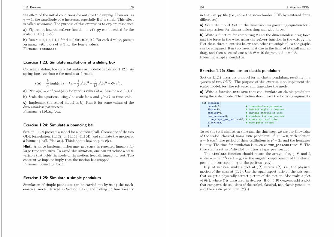
1.13 Exercises 105
the effect of the initial conditions die out due to damping. However, asγ → 1, the amplitude of u increases, especially if β is small. This effectis called resonance. The purpose of this exercise is to explore resonance.a) Figure out how the solver function in vib.py can be called for thescaled ODE (1.122).b) Run γ = 5, 1.5, 1.1, 1 for β = 0.005, 0.05, 0.2. For each β value, presentan image with plots of u(t) for the four γ values.Filename: resonance.
Exercise 1.23: Simulate oscillations of a sliding boxConsider a sliding box on a flat surface as modeled in Section 1.12.3. Asspring force we choose the nonlinear formula
s(u) = k
αtanh(αu) = ku+ 1
3α2ku3 + 2
15α4ku5 +O(u6) .
a) Plot g(u) = α−1 tanh(αu) for various values of α. Assume u ∈ [−1, 1].b) Scale the equations using I as scale for u and
√m/k as time scale.
c) Implement the scaled model in b). Run it for some values of thedimensionless parameters.Filename: sliding_box.
Exercise 1.24: Simulate a bouncing ballSection 1.12.9 presents a model for a bouncing ball. Choose one of the twoODE formulation, (1.152) or (1.153)-(1.154), and simulate the motion ofa bouncing ball. Plot h(t). Think about how to plot v(t).Hint. A naive implementation may get stuck in repeated impacts forlarge time step sizes. To avoid this situation, one can introduce a statevariable that holds the mode of the motion: free fall, impact, or rest. Twoconsecutive impacts imply that the motion has stopped.Filename: bouncing_ball.
Exercise 1.25: Simulate a simple pendulumSimulation of simple pendulum can be carried out by using the math-ematical model derived in Section 1.12.5 and calling up functionality
106 1 Vibration ODEs
in the vib.py file (i.e., solve the second-order ODE by centered finitedifferences).a) Scale the model. Set up the dimensionless governing equation for θand expressions for dimensionless drag and wire forces.b) Write a function for computing θ and the dimensionless drag forceand the force in the wire, using the solver function in the vib.py file.Plot these three quantities below each other (in subplots) so the graphscan be compared. Run two cases, first one in the limit of Θ small and nodrag, and then a second one with Θ = 40 degrees and α = 0.8.Filename: simple_pendulum.
Exercise 1.26: Simulate an elastic pendulumSection 1.12.7 describes a model for an elastic pendulum, resulting in asystem of two ODEs. The purpose of this exercise is to implement thescaled model, test the software, and generalize the model.a) Write a function simulate that can simulate an elastic pendulumusing the scaled model. The function should have the following arguments:
def simulate(beta=0.9, # dimensionless parameterTheta=30, # initial angle in degreesepsilon=0, # initial stretch of wirenum_periods=6, # simulate for num_periodstime_steps_per_period=60, # time step resolutionplot=True, # make plots or not):
To set the total simulation time and the time step, we use our knowledgeof the scaled, classical, non-elastic pendulum: u′′ + u = 0, with solutionu = Θ cos t. The period of these oscillations is P = 2π and the frequencyis unity. The time for simulation is taken as num_periods times P . Thetime step is set as P divided by time_steps_per_period.
The simulate function should return the arrays of x, y, θ, and t,where θ = tan−1(x/(1 − y)) is the angular displacement of the elasticpendulum corresponding to the position (x, y).
If plot is True, make a plot of y(t) versus x(t), i.e., the physicalmotion of the mass at (x, y). Use the equal aspect ratio on the axis suchthat we get a physically correct picture of the motion. Also make a plotof θ(t), where θ is measured in degrees. If Θ < 10 degrees, add a plotthat compares the solutions of the scaled, classical, non-elastic pendulumand the elastic pendulum (θ(t)).
1.13 Exercises 107
Although the mathematics here employs a bar over scaled quantities,the code should feature plain names x for x, y for y, and t for t (ratherthan x_bar, etc.). These variable names make the code easier to readand compare with the mathematics.Hint 1. Equal aspect ratio is set by plt.gca().set_aspect(’equal’)in Matplotlib (import matplotlib.pyplot as plt) and inSciTools by the command plt.plot(..., daspect=[1,1,1],daspectmode=’equal’) (provided you have done import scitools.stdas plt).Hint 2. If you want to use Odespy to solve the equations, order theODEs like ˙x, x,˙y, y such that odespy.EulerCromer can be applied.b) Write a test function for testing that Θ = 0 and ε = 0 gives x = y = 0for all times.c) Write another test function for checking that the pure vertical motionof the elastic pendulum is correct. Start with simplifying the ODEs forpure vertical motion and show that y(t) fulfills a vibration equation withfrequency
√β/(1− β). Set up the exact solution.
Write a test function that uses this special case to verify the simulatefunction. There will be numerical approximation errors present in theresults from simulate so you have to believe in correct results and set a(low) tolerance that corresponds to the computed maximum error. Use asmall ∆t to obtain a small numerical approximation error.d) Make a function demo(beta, Theta) for simulating an elastic pen-dulum with a given β parameter and initial angle Θ. Use 600 time stepsper period to get every accurate results, and simulate for 3 periods.Filename: elastic_pendulum.
Exercise 1.27: Simulate an elastic pendulum with airresistanceThis is a continuation Exercise 1.26. Air resistance on the body withmass m can be modeled by the force −1
2%CDA|v|v, where CD is a dragcoefficient (0.2 for a sphere), % is the density of air (1.2 kg m−3), A isthe cross section area (A = πR2 for a sphere, where R is the radius), andv is the velocity of the body. Include air resistance in the original model,scale the model, write a function simulate_drag that is a copy of thesimulate function from Exercise 1.26, but with the new ODEs included,and show plots of how air resistance influences the motion.Filename: elastic_pendulum_drag.
108 1 Vibration ODEs
Remarks. Test functions are challenging to construct for the prob-lem with air resistance. You can reuse the tests from Exercise 1.27 forsimulate_drag, but these tests does not verify the new terms arisingfrom air resistance.
Exercise 1.28: Implement the PEFRL algorithm
We consider the motion of a planet around a star (Section 1.12.10). Thesimplified case where one mass is very much bigger than the other andone object is at rest, results in the scaled ODE model
x+ (x2 + y2)−3/2x = 0,y + (x2 + y2)−3/2y = 0 .
a) It is easy to show that x(t) and y(t) go like sine and cosine functions.Use this idea to derive the exact solution.
b) One believes that a planet may orbit a star for billions of years. Weare now interested in how accurate methods we actually need for suchcalculations. A first task is to determine what the time interval of interestis in scaled units. Take the earth and sun as typical objects and find thecharacteristic time used in the scaling of the equations (tc =
√L3/(mG)),
where m is the mass of the sun, L is the distance between the sun and theearth, and G is the gravitational constant. Find the scaled time intervalcorresponding to one billion years.
c) Solve the equations using 4th-order Runge-Kutta and the Euler-Cromer methods. You may benefit from applying Odespy for this purpose.With each solver, simulate 10000 orbits and print the maximum positionerror and CPU time as a function of time step. Note that the maximumposition error does not necessarily occur at the end of the simulation.The position error achieved with each solver will depend heavily on thesize of the time step. Let the time step correspond to 200, 400, 800 and1600 steps per orbit, respectively. Are the results as expected? Explainbriefly. When you develop your program, have in mind that it will beextended with an implementation of the other algorithms (as requestedin d) and e) later) and experiments with this algorithm as well.
d) Implement a solver based on the PEFRL method from Section 1.10.11.Verify its 4th-order convergence using an equation u′′ + u = 0.
1.13 Exercises 109
e) The simulations done previously with the 4th-order Runge-Kuttaand Euler-Cromer are now to be repeated with the PEFRL solver, sothe code must be extended accordingly. Then run the simulations andcomment on the performance of PEFRL compared to the other two.
f) Use the PEFRL solver to simulate 100000 orbits with a fixed timestep corresponding to 1600 steps per period. Record the maximum errorwithin each subsequent group of 1000 orbits. Plot these errors and fit(least squares) a mathematical function to the data. Print also the totalCPU time spent for all 100000 orbits.
Now, predict the error and required CPU time for a simulation of 1billion years (orbits). Is it feasible on today’s computers to simulate theplanetary motion for one billion years?Filename: vib_PEFRL.
Remarks. This exercise investigates whether it is feasible to predictplanetary motion for the life time of a solar system.
Wave equations 2
A very wide range of physical processes lead to wave motion, wheresignals are propagated through a medium in space and time, normallywith little or no permanent movement of the medium itself. The shapeof the signals may undergo changes as they travel through matter, butusually not so much that the signals cannot be recognized at some laterpoint in space and time. Many types of wave motion can be described bythe equation utt = ∇· (c2∇u) + f , which we will solve in the forthcomingtext by finite difference methods.
2.1 Simulation of waves on a string
We begin our study of wave equations by simulating one-dimensionalwaves on a string, say on a guitar or violin. Let the string in the deformedstate coincide with the interval [0, L] on the x axis, and let u(x, t) be thedisplacement at time t in the y direction of a point initially at x. Thedisplacement function u is governed by the mathematical model
© 2016, Hans Petter Langtangen, Svein Linge. Released under CC Attribution 4.0 license
112 2 Wave equations
∂2u
∂t2= c2∂
2u
∂x2 , x ∈ (0, L), t ∈ (0, T ] (2.1)
u(x, 0) = I(x), x ∈ [0, L] (2.2)∂
∂tu(x, 0) = 0, x ∈ [0, L] (2.3)
u(0, t) = 0, t ∈ (0, T ] (2.4)u(L, t) = 0, t ∈ (0, T ] (2.5)
The constant c and the function I(x) must be prescribed.Equation (2.1) is known as the one-dimensional wave equation. Since
this PDE contains a second-order derivative in time, we need two initialconditions. The condition (2.2) specifies the initial shape of the string,I(x), and (2.3) expresses that the initial velocity of the string is zero. Inaddition, PDEs need boundary conditions, given here as (2.4) and (2.5).These two conditions specify that the string is fixed at the ends, i.e., thatthe displacement u is zero.
The solution u(x, t) varies in space and time and describes waves thatmove with velocity c to the left and right.
Sometimes we will use a more compact notation for the partial deriva-tives to save space:
ut = ∂u
∂t, utt = ∂2u
∂t2, (2.6)
and similar expressions for derivatives with respect to other variables.Then the wave equation can be written compactly as utt = c2uxx.
The PDE problem (2.1)-(2.5) will now be discretized in space andtime by a finite difference method.
2.1.1 Discretizing the domain
The temporal domain [0, T ] is represented by a finite number of meshpoints
0 = t0 < t1 < t2 < · · · < tNt−1 < tNt = T . (2.7)
Similarly, the spatial domain [0, L] is replaced by a set of mesh points
0 = x0 < x1 < x2 < · · · < xNx−1 < xNx = L . (2.8)
2.1 Simulation of waves on a string 113
One may view the mesh as two-dimensional in the x, t plane, consistingof points (xi, tn), with i = 0, . . . , Nx and n = 0, . . . , Nt.Uniform meshes. For uniformly distributed mesh points we can intro-duce the constant mesh spacings ∆t and ∆x. We have that
xi = i∆x, i = 0, . . . , Nx, tn = n∆t, n = 0, . . . , Nt . (2.9)
We also have that ∆x = xi − xi−1, i = 1, . . . , Nx, and ∆t = tn − tn−1,n = 1, . . . , Nt. Figure 2.1 displays a mesh in the x, t plane with Nt = 5,Nx = 5, and constant mesh spacings.
2.1.2 The discrete solutionThe solution u(x, t) is sought at the mesh points. We introduce the meshfunction uni , which approximates the exact solution at the mesh point(xi, tn) for i = 0, . . . , Nx and n = 0, . . . , Nt. Using the finite differencemethod, we shall develop algebraic equations for computing the meshfunction.
2.1.3 Fulfilling the equation at the mesh pointsIn the finite difference method, we relax the condition that (2.1) holdsat all points in the space-time domain (0, L)× (0, T ] to the requirementthat the PDE is fulfilled at the interior mesh points only:
∂2
∂t2u(xi, tn) = c2 ∂
2
∂x2u(xi, tn), (2.10)
for i = 1, . . . , Nx− 1 and n = 1, . . . , Nt− 1. For n = 0 we have the initialconditions u = I(x) and ut = 0, and at the boundaries i = 0, Nx we havethe boundary condition u = 0.
2.1.4 Replacing derivatives by finite differencesThe second-order derivatives can be replaced by central differences. Themost widely used difference approximation of the second-order derivativeis
∂2
∂t2u(xi, tn) ≈ un+1
i − 2uni + un−1i
∆t2.
114 2 Wave equations
It is convenient to introduce the finite difference operator notation
[DtDtu]ni = un+1i − 2uni + un−1
i
∆t2.
A similar approximation of the second-order derivative in the x directionreads
∂2
∂x2u(xi, tn) ≈ uni+1 − 2uni + uni−1∆x2 = [DxDxu]ni .
Algebraic version of the PDE. We can now replace the derivatives in(2.10) and get
un+1i − 2uni + un−1
i
∆t2= c2u
ni+1 − 2uni + uni−1
∆x2 , (2.11)
or written more compactly using the operator notation:
[DtDtu = c2DxDx]ni . (2.12)
Interpretation of the equation as a stencil. A characteristic featureof (2.11) is that it involves u values from neighboring points only: un+1
i ,uni±1, uni , and un−1
i . The circles in Figure 2.1 illustrate such neighboringmesh points that contribute to an algebraic equation. In this particularcase, we have sampled the PDE at the point (2, 2) and constructed (2.11),which then involves a coupling of unm11, u2
n, unm12, u23, and unm13.
The term stencil is often used about the algebraic equation at a meshpoint, and the geometry of a typical stencil is illustrated in Figure 2.1.One also often refers to the algebraic equations as discrete equations,(finite) difference equations or a finite difference scheme.
Algebraic version of the initial conditions. We also need to replace thederivative in the initial condition (2.3) by a finite difference approximation.A centered difference of the type
∂
∂tu(xi, t0) ≈ u1
i − u−1i
2∆t = [D2tu]0i ,
seems appropriate. Writing out this equation and ordering the terms give
u−1i = u1
i , i = 0, . . . , Nx . (2.13)
The other initial condition can be computed by
u0i = I(xi), i = 0, . . . , Nx .
2.1 Simulation of waves on a string 115
0
1
2
3
4
5
0 1 2 3 4 5
inde
x n
index i
Stencil at interior point
Fig. 2.1 Mesh in space and time. The circles show points connected in a finite differenceequation.
2.1.5 Formulating a recursive algorithm
We assume that uni and un−1i are available for i = 0, . . . , Nx. The only
unknown quantity in (2.11) is therefore un+1i , which we now can solve
for:
un+1i = −un−1
i + 2uni + C2 (uni+1 − 2uni + uni−1). (2.14)
We have here introduced the parameter
C = c∆t
∆x, (2.15)
known as the Courant number.
C is the key parameter in the discrete wave equation
We see that the discrete version of the PDE features only one pa-rameter, C, which is therefore the key parameter, together with Nx,that governs the quality of the numerical solution (see Section 2.10for details). Both the primary physical parameter c and the numeri-cal parameters ∆x and ∆t are lumped together in C. Note that Cis a dimensionless parameter.
116 2 Wave equations
Given that un−1i and uni are known for i = 0, . . . , Nx, we find new values
at the next time level by applying the formula (2.14) for i = 1, . . . , Nx−1.Figure 2.1 illustrates the points that are used to compute u3
2. For theboundary points, i = 0 and i = Nx, we apply the boundary conditionsun+1i = 0.Even though sound reasoning leads up to (2.14), there is still a minor
challenge with it that needs to be resolved. Think of the very firstcomputational step to be made. The scheme (2.14) is supposed to startat n = 1, which means that we compute u2 from u1 and u0. Unfortunately,we do not know the value of u1, so how to proceed? A standard procedurein such cases is to apply (2.14) also for n = 0. This immediately seemsstrange, since it involves u−1
i , which is an undefined quantity outsidethe time mesh (and the time domain). However, we can use the initialcondition (2.13) in combination with (2.14) when n = 0 to eliminate u−1
i
and arrive at a special formula for u1i :
u1i = u0
i −12C
2(u0i+1 − 2u0
i + u0i−1
). (2.16)
Figure 2.2 illustrates how (2.16) connects four instead of five points: u12,
u0n, unm10, and u0
3.
0
1
2
3
4
5
0 1 2 3 4 5
inde
x n
index i
Stencil at interior point
Fig. 2.2 Modified stencil for the first time step.
We can now summarize the computational algorithm:
2.1 Simulation of waves on a string 117
1. Compute u0i = I(xi) for i = 0, . . . , Nx
2. Compute u1i by (2.16) and set u1
i = 0 for the boundary points i = 0and i = Nx, for n = 1, 2, . . . , N − 1,
3. For each time level n = 1, 2, . . . , Nt − 1a. apply (2.14) to find un+1
i for i = 1, . . . , Nx − 1b. set un+1
i = 0 for the boundary points i = 0, i = Nx.
The algorithm essentially consists of moving a finite difference stencilthrough all the mesh points, which can be seen as an animation in a webpage1 or a movie file2.
2.1.6 Sketch of an implementation
The algorithm only involves the three most recent time levels, so we needonly three arrays for un+1
i , uni , and un−1i , i = 0, . . . , Nx. Storing all the
solutions in a two-dimensional array of size (Nx + 1)× (Nt + 1) would bepossible in this simple one-dimensional PDE problem, but is normallyout of the question in three-dimensional (3D) and large two-dimensional(2D) problems. We shall therefore, in all our PDE solving programs, havethe unknown in memory at as few time levels as possible.
In a Python implementation of this algorithm, we use the array el-ements u[i] to store un+1
i , u_n[i] to store uni , and u_nm1[i] to storeun−1i . Our naming convention is to use u for the unknown new spatial
field to be computed and have all previous time levels in a list u_n thatwe index as u_n, u_nm1, u_n[-2] and so on. For the wave equation, u_nhas just length 2.
The following Python snippet realizes the steps in the computationalalgorithm.
# Given mesh points as arrays x and t (x[i], t[n])dx = x[1] - x[0]dt = t[1] - t[0]C = c*dt/dx # Courant numberNt = len(t)-1C2 = C**2 # Help variable in the scheme
# Set initial condition u(x,0) = I(x)for i in range(0, Nx+1):
u_n[i] = I(x[i])
1 http://tinyurl.com/pu5uyfn/pub/pub/wave/html/mov-wave/D_stencil_gpl/index.html2 http://tinyurl.com/pu5uyfn/pub/pub/wave/html/mov-wave/D_stencil_gpl/movie.ogg
118 2 Wave equations
# Apply special formula for first step, incorporating du/dt=0for i in range(1, Nx):
u[i] = u_n[i] - \0.5*C**2(u_n[i+1] - 2*u_n[i] + u_n[i-1])
u[0] = 0; u[Nx] = 0 # Enforce boundary conditions
# Switch variables before next stepu_nm1[:], u_n[:] = u_n, u
for n in range(1, Nt):# Update all inner mesh points at time t[n+1]for i in range(1, Nx):
u[i] = 2u_n[i] - u_nm1[i] - \C**2(u_n[i+1] - 2*u_n[i] + u_n[i-1])
# Insert boundary conditionsu[0] = 0; u[Nx] = 0
# Switch variables before next stepu_nm1[:], u_n[:] = u_n, u
2.2 Verification
Before implementing the algorithm, it is convenient to add a sourceterm to the PDE (2.1), since that gives us more freedom in finding testproblems for verification. Physically, a source term acts as a generatorfor waves in the interior of the domain.
2.2.1 A slightly generalized model problem
We now address the following extended initial-boundary value problemfor one-dimensional wave phenomena:
utt = c2uxx + f(x, t), x ∈ (0, L), t ∈ (0, T ] (2.17)u(x, 0) = I(x), x ∈ [0, L] (2.18)ut(x, 0) = V (x), x ∈ [0, L] (2.19)u(0, t) = 0, t > 0 (2.20)u(L, t) = 0, t > 0 (2.21)
Sampling the PDE at (xi, tn) and using the same finite differenceapproximations as above, yields
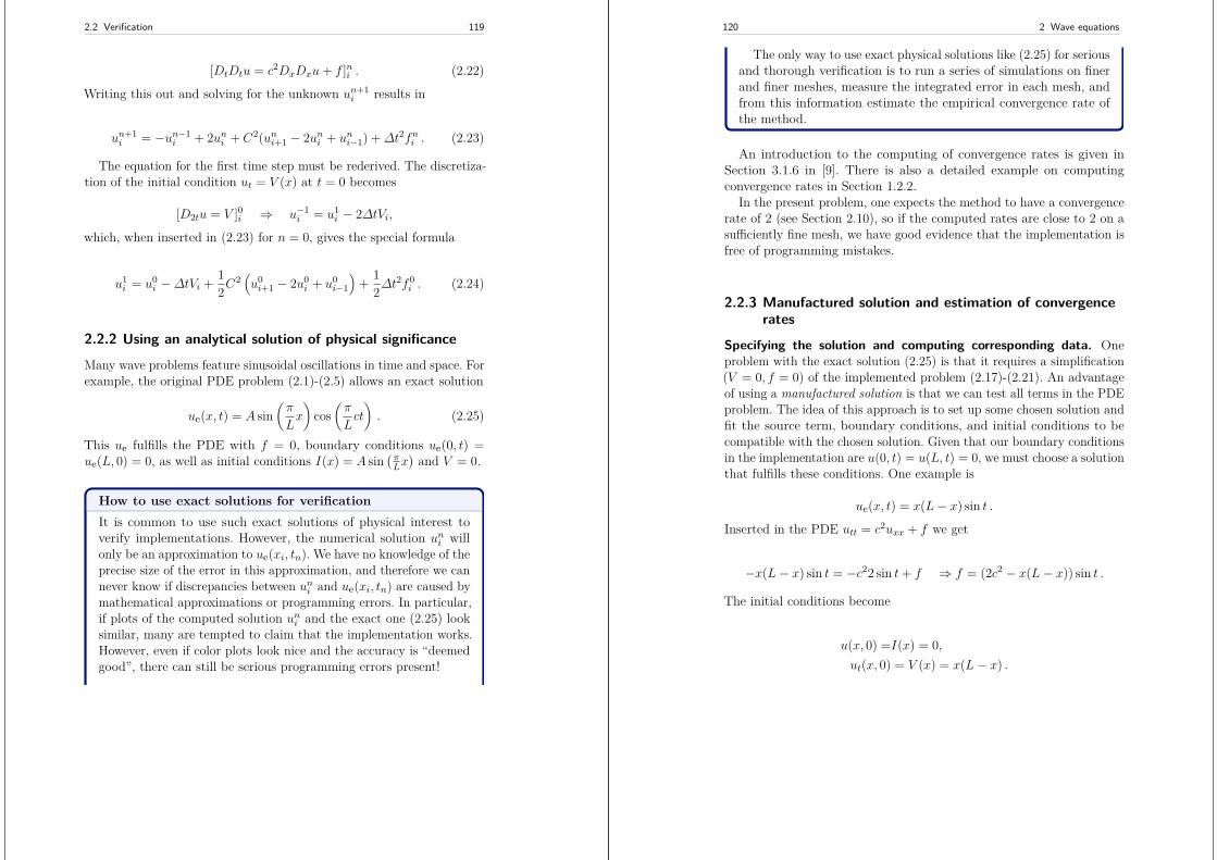
2.2 Verification 119
[DtDtu = c2DxDxu+ f ]ni . (2.22)
Writing this out and solving for the unknown un+1i results in
un+1i = −un−1
i + 2uni + C2(uni+1 − 2uni + uni−1) +∆t2fni . (2.23)
The equation for the first time step must be rederived. The discretiza-tion of the initial condition ut = V (x) at t = 0 becomes
[D2tu = V ]0i ⇒ u−1i = u1
i − 2∆tVi,
which, when inserted in (2.23) for n = 0, gives the special formula
u1i = u0
i −∆tVi + 12C
2(u0i+1 − 2u0
i + u0i−1
)+ 1
2∆t2f0i . (2.24)
2.2.2 Using an analytical solution of physical significance
Many wave problems feature sinusoidal oscillations in time and space. Forexample, the original PDE problem (2.1)-(2.5) allows an exact solution
ue(x, t) = A sin(π
Lx
)cos
(π
Lct
). (2.25)
This ue fulfills the PDE with f = 0, boundary conditions ue(0, t) =ue(L, 0) = 0, as well as initial conditions I(x) = A sin
(πLx)and V = 0.
How to use exact solutions for verificationIt is common to use such exact solutions of physical interest toverify implementations. However, the numerical solution uni willonly be an approximation to ue(xi, tn). We have no knowledge of theprecise size of the error in this approximation, and therefore we cannever know if discrepancies between uni and ue(xi, tn) are caused bymathematical approximations or programming errors. In particular,if plots of the computed solution uni and the exact one (2.25) looksimilar, many are tempted to claim that the implementation works.However, even if color plots look nice and the accuracy is “deemedgood”, there can still be serious programming errors present!
120 2 Wave equations
The only way to use exact physical solutions like (2.25) for seriousand thorough verification is to run a series of simulations on finerand finer meshes, measure the integrated error in each mesh, andfrom this information estimate the empirical convergence rate ofthe method.
An introduction to the computing of convergence rates is given inSection 3.1.6 in [9]. There is also a detailed example on computingconvergence rates in Section 1.2.2.
In the present problem, one expects the method to have a convergencerate of 2 (see Section 2.10), so if the computed rates are close to 2 on asufficiently fine mesh, we have good evidence that the implementation isfree of programming mistakes.
2.2.3 Manufactured solution and estimation of convergencerates
Specifying the solution and computing corresponding data. Oneproblem with the exact solution (2.25) is that it requires a simplification(V = 0, f = 0) of the implemented problem (2.17)-(2.21). An advantageof using a manufactured solution is that we can test all terms in the PDEproblem. The idea of this approach is to set up some chosen solution andfit the source term, boundary conditions, and initial conditions to becompatible with the chosen solution. Given that our boundary conditionsin the implementation are u(0, t) = u(L, t) = 0, we must choose a solutionthat fulfills these conditions. One example is
ue(x, t) = x(L− x) sin t .
Inserted in the PDE utt = c2uxx + f we get
−x(L− x) sin t = −c22 sin t+ f ⇒ f = (2c2 − x(L− x)) sin t .
The initial conditions become
u(x, 0) =I(x) = 0,ut(x, 0) = V (x) = x(L− x) .
2.2 Verification 121
Defining a single discretization parameter. To verify the code, wecompute the convergence rates in a series of simulations, letting eachsimulation use a finer mesh than the previous one. Such empirical estima-tion of convergence rates relies on an assumption that some measure Eof the numerical error is related to the discretization parameters through
E = Ct∆tr + Cx∆x
p,
where Ct, Cx, r, and p are constants. The constants r and p are known asthe convergence rates in time and space, respectively. From the accuracyin the finite difference approximations, we expect r = p = 2, since theerror terms are of order ∆t2 and ∆x2. This is confirmed by truncationerror analysis and other types of analysis.
By using an exact solution of the PDE problem, we will next computethe error measure E on a sequence of refined meshes and see if the ratesr = p = 2 are obtained. We will not be concerned with estimating theconstants Ct and Cx, simply because we are not interested in their values.
It is advantageous to introduce a single discretization parameter h =∆t = c∆x for some constant c. Since ∆t and ∆x are related through theCourant number, ∆t = C∆x/c, we set h = ∆t, and then ∆x = hc/C.Now the expression for the error measure is greatly simplified:
E = Ct∆tr+Cx∆xr = Cth
r+Cx(c
C
)rhr = Dhr, D = Ct+Cx
(c
C
)r.
Computing errors. We choose an initial discretization parameter h0 andrun experiments with decreasing h: hi = 2−ih0, i = 1, 2, . . . ,m. Halvingh in each experiment is not necessary, but it is a common choice. Foreach experiment we must record E and h. A standard choice of errormeasure is the `2 or `∞ norm of the error mesh function eni :
E = ||eni ||`2 =(∆t∆x
Nt∑
n=0
Nx∑
i=0(eni )2
) 12
, eni = ue(xi, tn)− uni , (2.26)
E = ||eni ||`∞ = maxi,n|ein| . (2.27)
In Python, one can compute∑i(eni )2 at each time step and accumulate
the value in some sum variable, say e2_sum. At the final time step onecan do sqrt(dt*dx*e2_sum). For the `∞ norm one must compare the
122 2 Wave equations
maximum error at a time level (e.max()) with the global maximum overthe time domain: e_max = max(e_max, e.max()).
An alternative error measure is to use a spatial norm at one time steponly, e.g., the end time T (n = Nt):
E = ||eni ||`2 =(∆x
Nx∑
i=0(eni )2
) 12
, eni = ue(xi, tn)− uni , (2.28)
E = ||eni ||`∞ = max0≤i≤Nx
|eni | . (2.29)
The important issue is that our error measure E must be one numberthat represents the error in the simulation.Computing rates. Let Ei be the error measure in experiment (mesh)number i and let hi be the corresponding discretization parameter (h).With the error model Ei = Dhri , we can estimate r by comparing twoconsecutive experiments:
Ei+1 = Dhri+1,
Ei = Dhri .
Dividing the two equations eliminates the (uninteresting) constant D.Thereafter, solving for r yields
r = lnEi+1/Eiln hi+1/hi
.
Since r depends on i, i.e., which simulations we compare, we add anindex to r: ri, where i = 0, . . . ,m − 2, if we have m experiments:(h0, E0), . . . , (hm−1, Em−1).
In our present discretization of the wave equation we expect r = 2,and hence the ri values should converge to 2 as i increases.
2.2.4 Constructing an exact solution of the discreteequations
With a manufactured or known analytical solution, as outlined above, wecan estimate convergence rates and see if they have the correct asymp-totic behavior. Experience shows that this is a quite good verificationtechnique in that many common bugs will destroy the convergence rates.
2.2 Verification 123
A significantly better test though, would be to check that the numer-ical solution is exactly what it should be. This will in general requireexact knowledge of the numerical error, which we do not normally have(although we in Section 2.10 establish such knowledge in simple cases).However, it is possible to look for solutions where we can show thatthe numerical error vanishes, i.e., the solution of the original continuousPDE problem is also a solution of the discrete equations. This propertyoften arises if the exact solution of the PDE is a lower-order polynomial.(Truncation error analysis leads to error measures that involve deriva-tives of the exact solution. In the present problem, the truncation errorinvolves 4th-order derivatives of u in space and time. Choosing u as apolynomial of degree three or less will therefore lead to vanishing error.)
We shall now illustrate the construction of an exact solution to boththe PDE itself and the discrete equations. Our chosen manufacturedsolution is quadratic in space and linear in time. More specifically, we set
ue(x, t) = x(L− x)(1 + 12 t), (2.30)
which by insertion in the PDE leads to f(x, t) = 2(1 + t)c2. This uefulfills the boundary conditions u = 0 and demands I(x) = x(L− x) andV (x) = 1
2x(L− x).To realize that the chosen ue is also an exact solution of the discrete
equations, we first remind ourselves that tn = n∆t before we establishthat
[DtDtt2]n = t2n+1 − 2t2n + t2n−1
∆t2= (n+ 1)2 − 2n2 + (n− 1)2 = 2,
(2.31)
[DtDtt]n = tn+1 − 2tn + tn−1∆t2
= ((n+ 1)− 2n+ (n− 1))∆t∆t2
= 0 .(2.32)
Hence,
[DtDtue]ni = xi(L− xi)[DtDt(1 + 12 t)]
n = xi(L− xi)12[DtDtt]n = 0 .
Similarly, we get that
124 2 Wave equations
[DxDxue]ni = (1 + 12 tn)[DxDx(xL− x2)]i
= (1 + 12 tn)[LDxDxx−DxDxx
2]i
= −2(1 + 12 tn) .
Now, fni = 2(1 + 12 tn)c2, which results in
[DtDtue − c2DxDxue − f ]ni = 0 + c22(1 + 12 tn) + 2(1 + 1
2 tn)c2 = 0 .
Moreover, ue(xi, 0) = I(xi), ∂ue/∂t = V (xi) at t = 0, and ue(x0, t) =ue(xNx , 0) = 0. Also the modified scheme for the first time step is fulfilledby ue(xi, tn).
Therefore, the exact solution ue(x, t) = x(L− x)(1 + t/2) of the PDEproblem is also an exact solution of the discrete problem. This meansthat we know beforehand what numbers the numerical algorithm shouldproduce. We can use this fact to check that the computed uni valuesfrom an implementation equals ue(xi, tn), within machine precision. Thisresult is valid regardless of the mesh spacings ∆x and ∆t! Nevertheless,there might be stability restrictions on ∆x and ∆t, so the test can onlybe run for a mesh that is compatible with the stability criterion (whichin the present case is C ≤ 1, to be derived later).
NoticeA product of quadratic or linear expressions in the various inde-pendent variables, as shown above, will often fulfill both the PDEproblem and the discrete equations, and can therefore be very usefulsolutions for verifying implementations.
However, for 1D wave equations of the type utt = c2uxx weshall see that there is always another much more powerful way ofgenerating exact solutions (which consists in just setting C = 1 (!),as shown in Section 2.10).
2.3 Implementation 125
2.3 Implementation
This section presents the complete computational algorithm, its imple-mentation in Python code, animation of the solution, and verification ofthe implementation.
A real implementation of the basic computational algorithm fromSections 2.1.5 and 2.1.6 can be encapsulated in a function, taking allthe input data for the problem as arguments. The physical input dataconsists of c, I(x), V (x), f(x, t), L, and T . The numerical input is themesh parameters ∆t and ∆x.
Instead of specifying ∆t and ∆x, we can specify one of them and theCourant number C instead, since having explicit control of the Courantnumber is convenient when investigating the numerical method. Manyfind it natural to prescribe the resolution of the spatial grid and set Nx.The solver function can then compute ∆t = CL/(cNx). However, forcomparing u(x, t) curves (as functions of x) for various Courant numbersit is more convenient to keep ∆t fixed for all C and let ∆x vary accordingto ∆x = c∆t/C. With ∆t fixed, all frames correspond to the same timet, and this simplifies animations that compare simulations with differentmesh resolutions. Plotting functions of x with different spatial resolutionis trivial, so it is easier to let ∆x vary in the simulations than ∆t.
2.3.1 Callback function for user-specific actions
The solution at all spatial points at a new time level is stored in an arrayu of length Nx + 1. We need to decide what to do with this solution, e.g.,visualize the curve, analyze the values, or write the array to file for lateruse. The decision about what to do is left to the user in the form of auser-supplied function
user_action(u, x, t, n)
where u is the solution at the spatial points x at time t[n]. Theuser_action function is called from the solver at each time level n.
If the user wants to plot the solution or store the solution at a timepoint, she needs to write such a function and take appropriate actionsinside it. We will show examples on many such user_action functions.
Since the solver function makes calls back to the user’s code via such afunction, this type of function is called a callback function. When writinggeneral software, like our solver function, which also needs to carry out
126 2 Wave equations
special problem- or solution-dependent actions (like visualization), itis a common technique to leave those actions to user-supplied callbackfunctions.
The callback function can be used to terminate the solution process ifthe user returns True. For example,
def my_user_action_function(u, x, t, n):return np.abs(u).max() > 10
is a callback function that will terminate the solver function of theamplitude of the waves exceed 10, which is here considered as a numericalinstability.
2.3.2 The solver functionA first attempt at a solver function is listed below.
import numpy as np
def solver(I, V, f, c, L, dt, C, T, user_action=None):"""Solve u_tt=c^2*u_xx + f on (0,L)x(0,T]."""Nt = int(round(T/dt))t = np.linspace(0, Nt*dt, Nt+1) # Mesh points in timedx = dt*c/float(C)Nx = int(round(L/dx))x = np.linspace(0, L, Nx+1) # Mesh points in spaceC2 = C**2 # Help variable in the scheme# Make sure dx and dt are compatible with x and tdx = x[1] - x[0]dt = t[1] - t[0]
if f is None or f == 0 :f = lambda x, t: 0
if V is None or V == 0:V = lambda x: 0
u = np.zeros(Nx+1) # Solution array at new time levelu_n = np.zeros(Nx+1) # Solution at 1 time level backu_nm1 = np.zeros(Nx+1) # Solution at 2 time levels back
import time; t0 = time.clock() # Measure CPU time
# Load initial condition into u_nfor i in range(0,Nx+1):
u_n[i] = I(x[i])
if user_action is not None:user_action(u_n, x, t, 0)
# Special formula for first time step
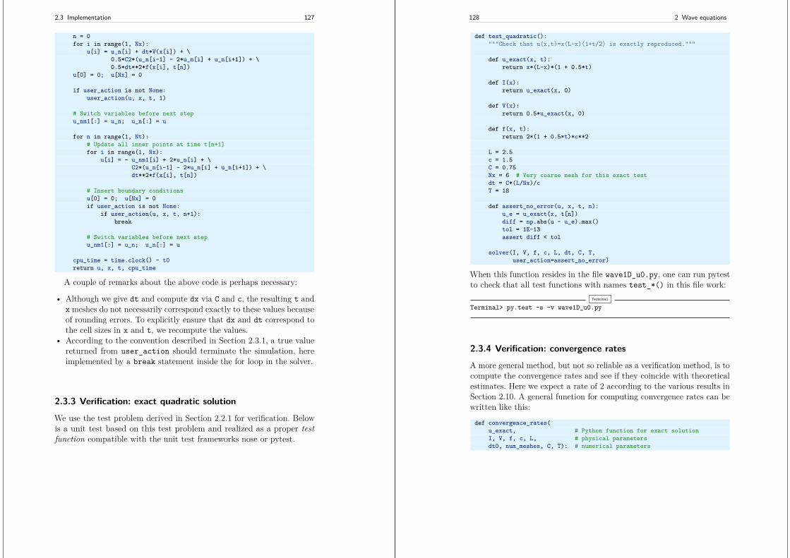
2.3 Implementation 127
n = 0for i in range(1, Nx):
u[i] = u_n[i] + dt*V(x[i]) + \0.5*C2*(u_n[i-1] - 2*u_n[i] + u_n[i+1]) + \0.5*dt**2*f(x[i], t[n])
u[0] = 0; u[Nx] = 0
if user_action is not None:user_action(u, x, t, 1)
# Switch variables before next stepu_nm1[:] = u_n; u_n[:] = u
for n in range(1, Nt):# Update all inner points at time t[n+1]for i in range(1, Nx):
u[i] = - u_nm1[i] + 2*u_n[i] + \C2*(u_n[i-1] - 2*u_n[i] + u_n[i+1]) + \dt**2*f(x[i], t[n])
# Insert boundary conditionsu[0] = 0; u[Nx] = 0if user_action is not None:
if user_action(u, x, t, n+1):break
# Switch variables before next stepu_nm1[:] = u_n; u_n[:] = u
cpu_time = time.clock() - t0return u, x, t, cpu_time
A couple of remarks about the above code is perhaps necessary:
• Although we give dt and compute dx via C and c, the resulting t andx meshes do not necessarily correspond exactly to these values becauseof rounding errors. To explicitly ensure that dx and dt correspond tothe cell sizes in x and t, we recompute the values.
• According to the convention described in Section 2.3.1, a true valuereturned from user_action should terminate the simulation, hereimplemented by a break statement inside the for loop in the solver.
2.3.3 Verification: exact quadratic solution
We use the test problem derived in Section 2.2.1 for verification. Belowis a unit test based on this test problem and realized as a proper testfunction compatible with the unit test frameworks nose or pytest.
128 2 Wave equations
def test_quadratic():"""Check that u(x,t)=x(L-x)(1+t/2) is exactly reproduced."""
def u_exact(x, t):return x*(L-x)*(1 + 0.5*t)
def I(x):return u_exact(x, 0)
def V(x):return 0.5*u_exact(x, 0)
def f(x, t):return 2*(1 + 0.5*t)*c**2
L = 2.5c = 1.5C = 0.75Nx = 6 # Very coarse mesh for this exact testdt = C*(L/Nx)/cT = 18
def assert_no_error(u, x, t, n):u_e = u_exact(x, t[n])diff = np.abs(u - u_e).max()tol = 1E-13assert diff < tol
solver(I, V, f, c, L, dt, C, T,user_action=assert_no_error)
When this function resides in the file wave1D_u0.py, one can run pytestto check that all test functions with names test_*() in this file work:
Terminal
Terminal> py.test -s -v wave1D_u0.py
2.3.4 Verification: convergence ratesA more general method, but not so reliable as a verification method, is tocompute the convergence rates and see if they coincide with theoreticalestimates. Here we expect a rate of 2 according to the various results inSection 2.10. A general function for computing convergence rates can bewritten like this:
def convergence_rates(u_exact, # Python function for exact solutionI, V, f, c, L, # physical parametersdt0, num_meshes, C, T): # numerical parameters
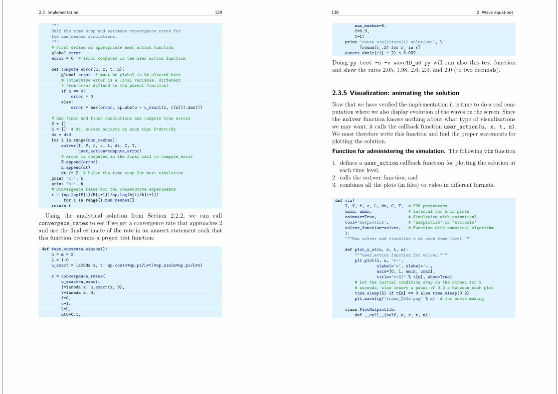
2.3 Implementation 129
"""Half the time step and estimate convergence rates forfor num_meshes simulations."""# First define an appropriate user action functionglobal errorerror = 0 # error computed in the user action function
def compute_error(u, x, t, n):global error # must be global to be altered here# (otherwise error is a local variable, different# from error defined in the parent function)if n == 0:
error = 0else:
error = max(error, np.abs(u - u_exact(x, t[n])).max())
# Run finer and finer resolutions and compute true errorsE = []h = [] # dt, solver adjusts dx such that C=dt*c/dxdt = dt0for i in range(num_meshes):
solver(I, V, f, c, L, dt, C, T,user_action=compute_error)
# error is computed in the final call to compute_errorE.append(error)h.append(dt)dt /= 2 # halve the time step for next simulation
print ’E:’, Eprint ’h:’, h# Convergence rates for two consecutive experimentsr = [np.log(E[i]/E[i-1])/np.log(h[i]/h[i-1])
for i in range(1,num_meshes)]return r
Using the analytical solution from Section 2.2.2, we can callconvergece_rates to see if we get a convergence rate that approaches 2and use the final estimate of the rate in an assert statement such thatthis function becomes a proper test function:
def test_convrate_sincos():n = m = 2L = 1.0u_exact = lambda x, t: np.cos(m*np.pi/L*t)*np.sin(m*np.pi/L*x)
r = convergence_rates(u_exact=u_exact,I=lambda x: u_exact(x, 0),V=lambda x: 0,f=0,c=1,L=L,dt0=0.1,
130 2 Wave equations
num_meshes=6,C=0.9,T=1)
print ’rates sin(x)*cos(t) solution:’, \[round(r_,2) for r_ in r]
assert abs(r[-1] - 2) < 0.002
Doing py.test -s -v wave1D_u0.py will run also this test functionand show the rates 2.05, 1.98, 2.0, 2.0, and 2.0 (to two decimals).
2.3.5 Visualization: animating the solutionNow that we have verified the implementation it is time to do a real com-putation where we also display evolution of the waves on the screen. Sincethe solver function knows nothing about what type of visualizationswe may want, it calls the callback function user_action(u, x, t, n).We must therefore write this function and find the proper statements forplotting the solution.Function for administering the simulation. The following viz function
1. defines a user_action callback function for plotting the solution ateach time level,
2. calls the solver function, and3. combines all the plots (in files) to video in different formats.
def viz(I, V, f, c, L, dt, C, T, # PDE parametersumin, umax, # Interval for u in plotsanimate=True, # Simulation with animation?tool=’matplotlib’, # ’matplotlib’ or ’scitools’solver_function=solver, # Function with numerical algorithm):"""Run solver and visualize u at each time level."""
def plot_u_st(u, x, t, n):"""user_action function for solver."""plt.plot(x, u, ’r-’,
xlabel=’x’, ylabel=’u’,axis=[0, L, umin, umax],title=’t=%f’ % t[n], show=True)
# Let the initial condition stay on the screen for 2# seconds, else insert a pause of 0.2 s between each plottime.sleep(2) if t[n] == 0 else time.sleep(0.2)plt.savefig(’frame_%04d.png’ % n) # for movie making
class PlotMatplotlib:def __call__(self, u, x, t, n):
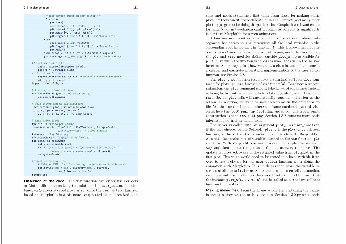
2.3 Implementation 131
"""user_action function for solver."""if n == 0:
plt.ion()self.lines = plt.plot(x, u, ’r-’)plt.xlabel(’x’); plt.ylabel(’u’)plt.axis([0, L, umin, umax])plt.legend([’t=%f’ % t[n]], loc=’lower left’)
else:self.lines[0].set_ydata(u)plt.legend([’t=%f’ % t[n]], loc=’lower left’)plt.draw()
time.sleep(2) if t[n] == 0 else time.sleep(0.2)plt.savefig(’tmp_%04d.png’ % n) # for movie making
if tool == ’matplotlib’:import matplotlib.pyplot as pltplot_u = PlotMatplotlib()
elif tool == ’scitools’:import scitools.std as plt # scitools.easyviz interfaceplot_u = plot_u_st
import time, glob, os
# Clean up old movie framesfor filename in glob.glob(’tmp_*.png’):
os.remove(filename)
# Call solver and do the simulatonuser_action = plot_u if animate else Noneu, x, t, cpu = solver_function(
I, V, f, c, L, dt, C, T, user_action)
# Make video filesfps = 4 # frames per secondcodec2ext = dict(flv=’flv’, libx264=’mp4’, libvpx=’webm’,
libtheora=’ogg’) # video formatsfilespec = ’tmp_%04d.png’movie_program = ’ffmpeg’ # or ’avconv’for codec in codec2ext:
ext = codec2ext[codec]cmd = ’%(movie_program)s -r %(fps)d -i %(filespec)s ’\
’-vcodec %(codec)s movie.%(ext)s’ % vars()os.system(cmd)
if tool == ’scitools’:# Make an HTML play for showing the animation in a browserplt.movie(’tmp_*.png’, encoder=’html’, fps=fps,
output_file=’movie.html’)return cpu
Dissection of the code. The viz function can either use SciToolsor Matplotlib for visualizing the solution. The user_action functionbased on SciTools is called plot_u_st, while the user_action functionbased on Matplotlib is a bit more complicated as it is realized as a
132 2 Wave equations
class and needs statements that differ from those for making staticplots. SciTools can utilize both Matplotlib and Gnuplot (and many otherplotting programs) for doing the graphics, but Gnuplot is a relevant choicefor large Nx or in two-dimensional problems as Gnuplot is significantlyfaster than Matplotlib for screen animations.
A function inside another function, like plot_u_st in the above codesegment, has access to and remembers all the local variables in thesurrounding code inside the viz function (!). This is known in computerscience as a closure and is very convenient to program with. For example,the plt and time modules defined outside plot_u are accessible forplot_u_st when the function is called (as user_action) in the solverfunction. Some may think, however, that a class instead of a closure isa cleaner and easier-to-understand implementation of the user actionfunction, see Section 2.8.
The plot_u_st function just makes a standard SciTools plot com-mand for plotting u as a function of x at time t[n]. To achieve a smoothanimation, the plot command should take keyword arguments insteadof being broken into separate calls to xlabel, ylabel, axis, time, andshow. Several plot calls will automatically cause an animation on thescreen. In addition, we want to save each frame in the animation tofile. We then need a filename where the frame number is padded withzeros, here tmp_0000.png, tmp_0001.png, and so on. The proper printfconstruction is then tmp_%04d.png. Section 1.3.2 contains more basicinformation on making animations.
The solver is called with an argument plot_u as user_function.If the user chooses to use SciTools, plot_u is the plot_u_st callbackfunction, but for Matplotlib it is an instance of the class PlotMatplotlib.Also this class makes use of variables defined in the viz function: pltand time. With Matplotlib, one has to make the first plot the standardway, and then update the y data in the plot at every time level. Theupdate requires active use of the returned value from plt.plot in thefirst plot. This value would need to be stored in a local variable if wewere to use a closure for the user_action function when doing theanimation with Matplotlib. It is much easier to store the variable asa class attribute self.lines. Since the class is essentially a function,we implement the function as the special method __call__ such thatthe instance plot_u(u, x, t, n) can be called as a standard callbackfunction from solver.Making movie files. From the frame_*.png files containing the framesin the animation we can make video files. Section 1.3.2 presents basic
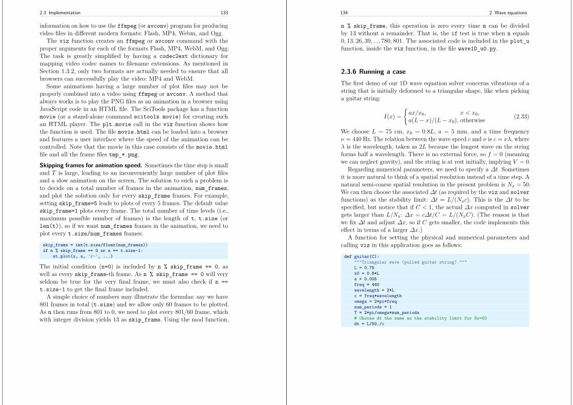
2.3 Implementation 133
information on how to use the ffmpeg (or avconv) program for producingvideo files in different modern formats: Flash, MP4, Webm, and Ogg.
The viz function creates an ffmpeg or avconv command with theproper arguments for each of the formats Flash, MP4, WebM, and Ogg.The task is greatly simplified by having a codec2ext dictionary formapping video codec names to filename extensions. As mentioned inSection 1.3.2, only two formats are actually needed to ensure that allbrowsers can successfully play the video: MP4 and WebM.
Some animations having a large number of plot files may not beproperly combined into a video using ffmpeg or avconv. A method thatalways works is to play the PNG files as an animation in a browser usingJavaScript code in an HTML file. The SciTools package has a functionmovie (or a stand-alone command scitools movie) for creating suchan HTML player. The plt.movie call in the viz function shows howthe function is used. The file movie.html can be loaded into a browserand features a user interface where the speed of the animation can becontrolled. Note that the movie in this case consists of the movie.htmlfile and all the frame files tmp_*.png.
Skipping frames for animation speed. Sometimes the time step is smalland T is large, leading to an inconveniently large number of plot filesand a slow animation on the screen. The solution to such a problem isto decide on a total number of frames in the animation, num_frames,and plot the solution only for every skip_frame frames. For example,setting skip_frame=5 leads to plots of every 5 frames. The default valueskip_frame=1 plots every frame. The total number of time levels (i.e.,maximum possible number of frames) is the length of t, t.size (orlen(t)), so if we want num_frames frames in the animation, we need toplot every t.size/num_frames frames:
skip_frame = int(t.size/float(num_frames))if n % skip_frame == 0 or n == t.size-1:
st.plot(x, u, ’r-’, ...)
The initial condition (n=0) is included by n % skip_frame == 0, aswell as every skip_frame-th frame. As n % skip_frame == 0 will veryseldom be true for the very final frame, we must also check if n ==t.size-1 to get the final frame included.
A simple choice of numbers may illustrate the formulas: say we have801 frames in total (t.size) and we allow only 60 frames to be plotted.As n then runs from 801 to 0, we need to plot every 801/60 frame, whichwith integer division yields 13 as skip_frame. Using the mod function,
134 2 Wave equations
n % skip_frame, this operation is zero every time n can be dividedby 13 without a remainder. That is, the if test is true when n equals0, 13, 26, 39, ..., 780, 801. The associated code is included in the plot_ufunction, inside the viz function, in the file wave1D_u0.py.
2.3.6 Running a caseThe first demo of our 1D wave equation solver concerns vibrations of astring that is initially deformed to a triangular shape, like when pickinga guitar string:
I(x) =ax/x0, x < x0,a(L− x)/(L− x0), otherwise (2.33)
We choose L = 75 cm, x0 = 0.8L, a = 5 mm, and a time frequencyν = 440 Hz. The relation between the wave speed c and ν is c = νλ, whereλ is the wavelength, taken as 2L because the longest wave on the stringforms half a wavelength. There is no external force, so f = 0 (meaningwe can neglect gravity), and the string is at rest initially, implying V = 0.
Regarding numerical parameters, we need to specify a ∆t. Sometimesit is more natural to think of a spatial resolution instead of a time step. Anatural semi-coarse spatial resolution in the present problem is Nx = 50.We can then choose the associated ∆t (as required by the viz and solverfunctions) as the stability limit: ∆t = L/(Nxc). This is the ∆t to bespecified, but notice that if C < 1, the actual ∆x computed in solvergets larger than L/Nx: ∆x = c∆t/C = L/(NxC). (The reason is thatwe fix ∆t and adjust ∆x, so if C gets smaller, the code implements thiseffect in terms of a larger ∆x.)
A function for setting the physical and numerical parameters andcalling viz in this application goes as follows:
def guitar(C):"""Triangular wave (pulled guitar string)."""L = 0.75x0 = 0.8*La = 0.005freq = 440wavelength = 2*Lc = freq*wavelengthomega = 2*pi*freqnum_periods = 1T = 2*pi/omega*num_periods# Choose dt the same as the stability limit for Nx=50dt = L/50./c
2.3 Implementation 135
def I(x):return a*x/x0 if x < x0 else a/(L-x0)*(L-x)
umin = -1.2*a; umax = -umincpu = viz(I, 0, 0, c, L, dt, C, T, umin, umax,
animate=True, tool=’scitools’)
The associated program has the name wave1D_u0.py. Run the programand watch the movie of the vibrating string3. The string should ideallyconsist of straight segments, but these are somewhat wavy due to nu-merical approximation. Run the case with the wave1D_u0.py code andC = 1 to see the exact solution.
2.3.7 Working with a scaled PDE model
Depending on the model, it may be a substantial job to establish consis-tent and relevant physical parameter values for a case. The guitar stringexample illustrates the point. However, by scaling the mathematicalproblem we can often reduce the need to estimate physical parametersdramatically. The scaling technique consists of introducing new indepen-dent and dependent variables, with the aim that the absolute values ofthese lie in [0, 1]. We introduce the dimensionless variables (details arefound in Section 3.1.1 in [11]
x = x
L, t = c
Lt, u = u
a.
Here, L is a typical length scale, e.g., the length of the domain, and ais a typical size of u, e.g., determined from the initial condition: a =maxx |I(x)|.
We get by the chain rule that
∂u
∂t= ∂
∂t(au) dt
dt= ac
L
∂u
∂t.
Similarly,
∂u
∂x= a
L
∂u
∂x.
Inserting the dimensionless variables in the PDE gives, in case f = 0,
3 http://tinyurl.com/pu5uyfn/pub/pub/wave/html/mov-wave/guitar_C0.8/movie.html
136 2 Wave equations
a2c2
L2∂2u
∂t2= a2c2
L2∂2u
∂x2 .
Dropping the bars, we arrive at the scaled PDE
∂2u
∂t2= ∂2u
∂x2 , x ∈ (0, 1), t ∈ (0, cT/L), (2.34)
which has no parameter c2 anymore. The initial conditions are scaled as
au(x, 0) = I(Lx)
and
a
L/c
∂u
∂t(x, 0) = V (Lx),
resulting in
u(x, 0) = I(Lx)maxx |I(x)| ,
∂u
∂t(x, 0) = L
acV (Lx) .
In the common case V = 0 we see that there are no physical parametersto be estimated in the PDE model!
If we have a program implemented for the physical wave equation withdimensions, we can obtain the dimensionless, scaled version by settingc = 1. The initial condition of a guitar string, given in (2.33), gets itsscaled form by choosing a = 1, L = 1, and x0 ∈ [0, 1]. This means thatwe only need to decide on the x0 value as a fraction of unity, becausethe scaled problem corresponds to setting all other parameters to unity.In the code we can just set a=c=L=1, x0=0.8, and there is no need tocalculate with wavelengths and frequencies to estimate c!
The only non-trivial parameter to estimate in the scaled problem isthe final end time of the simulation, or more precisely, how it relates toperiods in periodic solutions in time, since we often want to express theend time as a certain number of periods. The period in the dimensionlessproblem is 2, so the end time can be set to the desired number of periodstimes 2.
Why the dimensionless period is 2 can be explained by the followingreasoning. Suppose that u behaves as cos(ωt) in time in the originalproblem with dimensions. The corresponding period is then P = 2π/ω,but we need to estimate ω. A typical solution of the wave equation isu(x, t) = A cos(kx) cos(ωt), where A is an amplitude and k is relatedto the wave length λ in space: λ = 2π/k. Both λ and A will be given
2.4 Vectorization 137
by the initial condition I(x). Inserting this u(x, t) in the PDE yields−ω2 = −c2k2, i.e., ω = kc. The period is therefore P = 2π/(kc). If theboundary conditions are u(0, t) = u(L, t), we need to have kL = nπfor integer n. The period becomes P = 2L/nc. The longest period isP = 2L/c. The dimensionless period P is obtained by dividing P bythe time scale L/c, which results in P = 2. Shorter waves in the initialcondition will have a dimensionless shorter period P = 2/n (n > 1).
2.4 Vectorization
The computational algorithm for solving the wave equation visits onemesh point at a time and evaluates a formula for the new value un+1
i
at that point. Technically, this is implemented by a loop over arrayelements in a program. Such loops may run slowly in Python (and similarinterpreted languages such as R and MATLAB). One technique forspeeding up loops is to perform operations on entire arrays instead ofworking with one element at a time. This is referred to as vectorization,vector computing, or array computing. Operations on whole arrays arepossible if the computations involving each element is independent of eachother and therefore can, at least in principle, be performed simultaneously.That is, vectorization not only speeds up the code on serial computers,but also makes it easy to exploit parallel computing. Actually, there arePython tools like Numba4 that can automatically turn vectorized codeinto parallel code.
2.4.1 Operations on slices of arrays
Efficient computing with numpy arrays demands that we avoid loops andcompute with entire arrays at once (or at least large portions of them).Consider this calculation of differences di = ui+1 − ui:
n = u.sizefor i in range(0, n-1):
d[i] = u[i+1] - u[i]
All the differences here are independent of each other. The computa-tion of d can therefore alternatively be done by subtracting the array(u0, un, . . . , un−1) from the array where the elements are shifted one index
4 http://numba.pydata.org
138 2 Wave equations
upwards: (un, unm1, . . . , un), see Figure 2.3. The former subset of thearray can be expressed by u[0:n-1], u[0:-1], or just u[:-1], meaningfrom index 0 up to, but not including, the last element (-1). The lattersubset is obtained by u[1:n] or u[1:], meaning from index 1 and therest of the array. The computation of d can now be done without anexplicit Python loop:
d = u[1:] - u[:-1]
or with explicit limits if desired:
d = u[1:n] - u[0:n-1]
Indices with a colon, going from an index to (but not including) anotherindex are called slices. With numpy arrays, the computations are stilldone by loops, but in efficient, compiled, highly optimized C or Fortrancode. Such loops are sometimes referred to as vectorized loops. Suchloops can also easily be distributed among many processors on parallelcomputers. We say that the scalar code above, working on an element(a scalar) at a time, has been replaced by an equivalent vectorized code.The process of vectorizing code is called vectorization.
− −−−
0 1 2 3 4
0 1 2 3 4Fig. 2.3 Illustration of subtracting two slices of two arrays.
Test your understanding
Newcomers to vectorization are encouraged to choose a small arrayu, say with five elements, and simulate with pen and paper both theloop version and the vectorized version above.
Finite difference schemes basically contain differences between arrayelements with shifted indices. As an example, consider the updatingformula
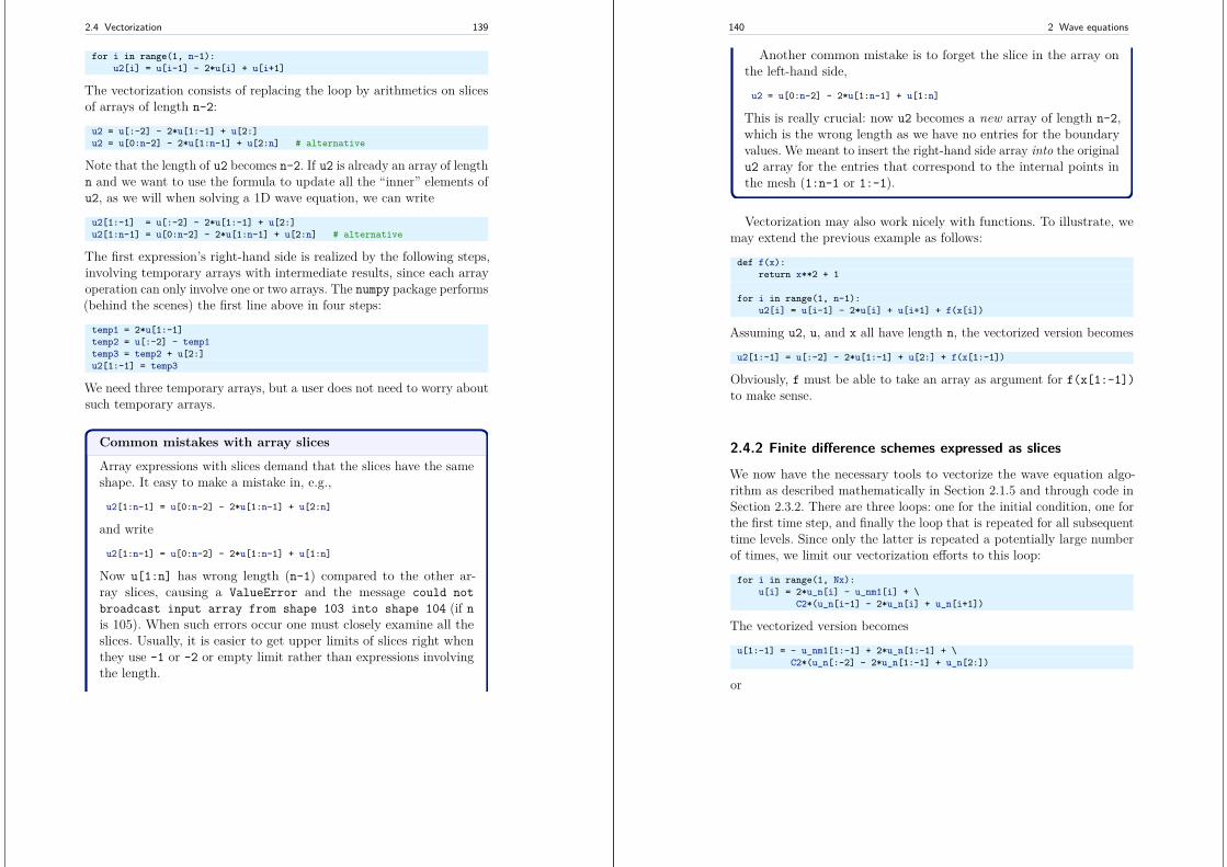
2.4 Vectorization 139
for i in range(1, n-1):u2[i] = u[i-1] - 2*u[i] + u[i+1]
The vectorization consists of replacing the loop by arithmetics on slicesof arrays of length n-2:
u2 = u[:-2] - 2*u[1:-1] + u[2:]u2 = u[0:n-2] - 2*u[1:n-1] + u[2:n] # alternative
Note that the length of u2 becomes n-2. If u2 is already an array of lengthn and we want to use the formula to update all the “inner” elements ofu2, as we will when solving a 1D wave equation, we can write
u2[1:-1] = u[:-2] - 2*u[1:-1] + u[2:]u2[1:n-1] = u[0:n-2] - 2*u[1:n-1] + u[2:n] # alternative
The first expression’s right-hand side is realized by the following steps,involving temporary arrays with intermediate results, since each arrayoperation can only involve one or two arrays. The numpy package performs(behind the scenes) the first line above in four steps:
temp1 = 2*u[1:-1]temp2 = u[:-2] - temp1temp3 = temp2 + u[2:]u2[1:-1] = temp3
We need three temporary arrays, but a user does not need to worry aboutsuch temporary arrays.
Common mistakes with array slices
Array expressions with slices demand that the slices have the sameshape. It easy to make a mistake in, e.g.,
u2[1:n-1] = u[0:n-2] - 2*u[1:n-1] + u[2:n]
and write
u2[1:n-1] = u[0:n-2] - 2*u[1:n-1] + u[1:n]
Now u[1:n] has wrong length (n-1) compared to the other ar-ray slices, causing a ValueError and the message could notbroadcast input array from shape 103 into shape 104 (if nis 105). When such errors occur one must closely examine all theslices. Usually, it is easier to get upper limits of slices right whenthey use -1 or -2 or empty limit rather than expressions involvingthe length.
140 2 Wave equations
Another common mistake is to forget the slice in the array onthe left-hand side,
u2 = u[0:n-2] - 2*u[1:n-1] + u[1:n]
This is really crucial: now u2 becomes a new array of length n-2,which is the wrong length as we have no entries for the boundaryvalues. We meant to insert the right-hand side array into the originalu2 array for the entries that correspond to the internal points inthe mesh (1:n-1 or 1:-1).
Vectorization may also work nicely with functions. To illustrate, wemay extend the previous example as follows:
def f(x):return x**2 + 1
for i in range(1, n-1):u2[i] = u[i-1] - 2*u[i] + u[i+1] + f(x[i])
Assuming u2, u, and x all have length n, the vectorized version becomes
u2[1:-1] = u[:-2] - 2*u[1:-1] + u[2:] + f(x[1:-1])
Obviously, f must be able to take an array as argument for f(x[1:-1])to make sense.
2.4.2 Finite difference schemes expressed as slices
We now have the necessary tools to vectorize the wave equation algo-rithm as described mathematically in Section 2.1.5 and through code inSection 2.3.2. There are three loops: one for the initial condition, one forthe first time step, and finally the loop that is repeated for all subsequenttime levels. Since only the latter is repeated a potentially large numberof times, we limit our vectorization efforts to this loop:
for i in range(1, Nx):u[i] = 2*u_n[i] - u_nm1[i] + \
C2*(u_n[i-1] - 2*u_n[i] + u_n[i+1])
The vectorized version becomes
u[1:-1] = - u_nm1[1:-1] + 2*u_n[1:-1] + \C2*(u_n[:-2] - 2*u_n[1:-1] + u_n[2:])
or
2.4 Vectorization 141
u[1:Nx] = 2*u_n[1:Nx]- u_nm1[1:Nx] + \C2*(u_n[0:Nx-1] - 2*u_n[1:Nx] + u_n[2:Nx+1])
The program wave1D_u0v.py contains a new version of the functionsolver where both the scalar and the vectorized loops are included (theargument version is set to scalar or vectorized, respectively).
2.4.3 Verification
We may reuse the quadratic solution ue(x, t) = x(L − x)(1 + 12 t) for
verifying also the vectorized code. A test function can now verify both thescalar and the vectorized version. Moreover, we may use a user_actionfunction that compares the computed and exact solution at each timelevel and performs a test:
def test_quadratic():"""Check the scalar and vectorized versions fora quadratic u(x,t)=x(L-x)(1+t/2) that is exactly reproduced."""# The following function must work for x as array or scalaru_exact = lambda x, t: x*(L - x)*(1 + 0.5*t)I = lambda x: u_exact(x, 0)V = lambda x: 0.5*u_exact(x, 0)# f is a scalar (zeros_like(x) works for scalar x too)f = lambda x, t: np.zeros_like(x) + 2*c**2*(1 + 0.5*t)
L = 2.5c = 1.5C = 0.75Nx = 3 # Very coarse mesh for this exact testdt = C*(L/Nx)/cT = 18
def assert_no_error(u, x, t, n):u_e = u_exact(x, t[n])tol = 1E-13diff = np.abs(u - u_e).max()assert diff < tol
solver(I, V, f, c, L, dt, C, T,user_action=assert_no_error, version=’scalar’)
solver(I, V, f, c, L, dt, C, T,user_action=assert_no_error, version=’vectorized’)
142 2 Wave equations
Lambda functionsThe code segment above demonstrates how to achieve very compactcode, without degraded readability, by use of lambda functions forthe various input parameters that require a Python function. Inessence,
f = lambda x, t: L*(x-t)**2
is equivalent to
def f(x, t):return L(x-t)**2
Note that lambda functions can just contain a single expression andno statements.
One advantage with lambda functions is that they can be useddirectly in calls:
solver(I=lambda x: sin(pi*x/L), V=0, f=0, ...)
2.4.4 Efficiency measurementsThe wave1D_u0v.py contains our new solver function with both scalarand vectorized code. For comparing the efficiency of scalar versus vector-ized code, we need a viz function as discussed in Section 2.3.5. All of thisviz function can be reused, except the call to solver_function. Thiscall lacks the parameter version, which we want to set to vectorizedand scalar for our efficiency measurements.
One solution is to copy the viz code from wave1D_u0 intowave1D_u0v.py and add a version argument to the solver_functioncall. Taking into account how much animation code we then duplicate,this is not a good idea. Alternatively, introducing the version argu-ment in wave1D_u0.viz, so that this function can be imported intowave1D_u0v.py, is not a good solution either, since version has nomeaning in that file. We need better ideas!Solution 1. Calling viz in wave1D_u0 with solver_function asour new solver in wave1D_u0v works fine, since this solver hasversion=’vectorized’ as default value. The problem arises whenwe want to test version=’scalar’. The simplest solution is thento use wave1D_u0.solver instead. We make a new viz function in
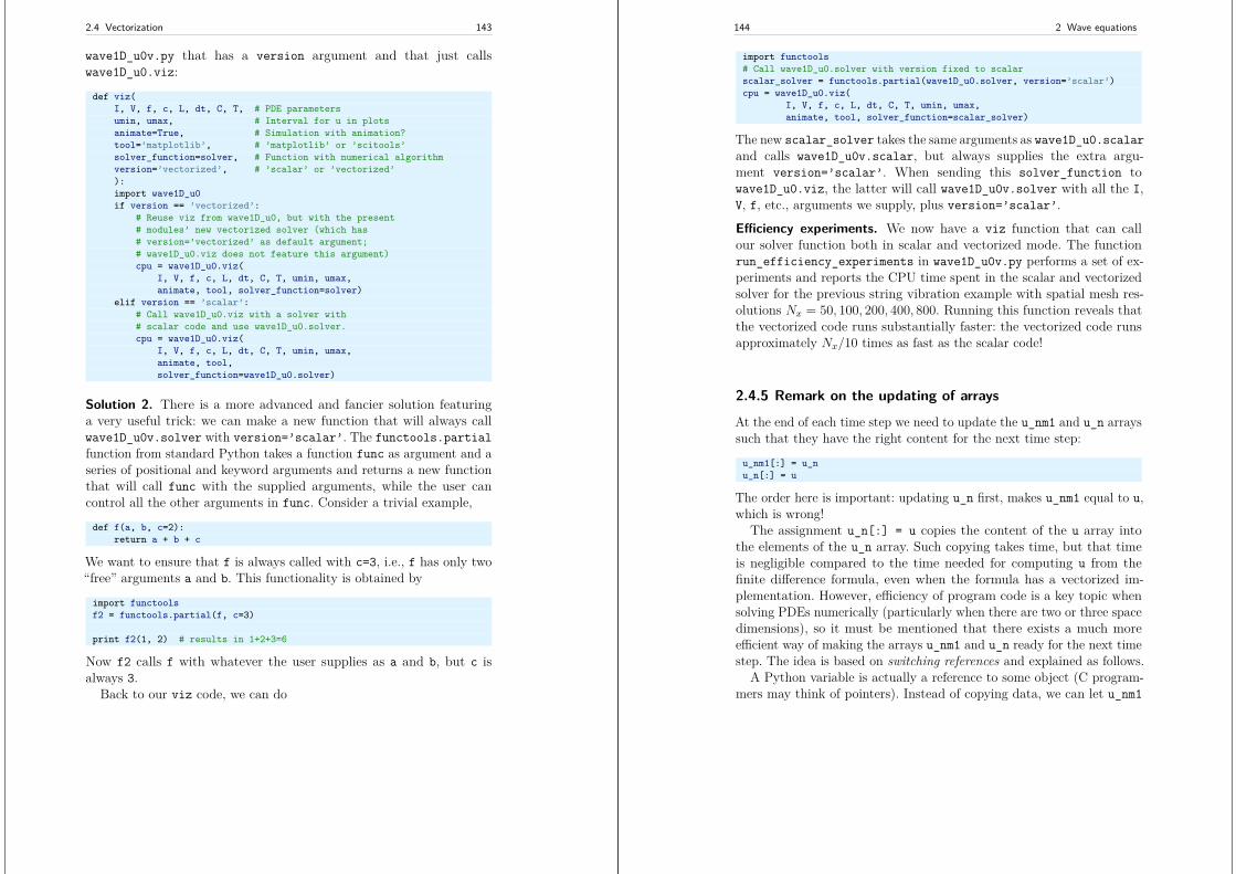
2.4 Vectorization 143
wave1D_u0v.py that has a version argument and that just callswave1D_u0.viz:
def viz(I, V, f, c, L, dt, C, T, # PDE parametersumin, umax, # Interval for u in plotsanimate=True, # Simulation with animation?tool=’matplotlib’, # ’matplotlib’ or ’scitools’solver_function=solver, # Function with numerical algorithmversion=’vectorized’, # ’scalar’ or ’vectorized’):import wave1D_u0if version == ’vectorized’:
# Reuse viz from wave1D_u0, but with the present# modules’ new vectorized solver (which has# version=’vectorized’ as default argument;# wave1D_u0.viz does not feature this argument)cpu = wave1D_u0.viz(
I, V, f, c, L, dt, C, T, umin, umax,animate, tool, solver_function=solver)
elif version == ’scalar’:# Call wave1D_u0.viz with a solver with# scalar code and use wave1D_u0.solver.cpu = wave1D_u0.viz(
I, V, f, c, L, dt, C, T, umin, umax,animate, tool,solver_function=wave1D_u0.solver)
Solution 2. There is a more advanced and fancier solution featuringa very useful trick: we can make a new function that will always callwave1D_u0v.solver with version=’scalar’. The functools.partialfunction from standard Python takes a function func as argument and aseries of positional and keyword arguments and returns a new functionthat will call func with the supplied arguments, while the user cancontrol all the other arguments in func. Consider a trivial example,
def f(a, b, c=2):return a + b + c
We want to ensure that f is always called with c=3, i.e., f has only two“free” arguments a and b. This functionality is obtained by
import functoolsf2 = functools.partial(f, c=3)
print f2(1, 2) # results in 1+2+3=6
Now f2 calls f with whatever the user supplies as a and b, but c isalways 3.
Back to our viz code, we can do
144 2 Wave equations
import functools# Call wave1D_u0.solver with version fixed to scalarscalar_solver = functools.partial(wave1D_u0.solver, version=’scalar’)cpu = wave1D_u0.viz(
I, V, f, c, L, dt, C, T, umin, umax,animate, tool, solver_function=scalar_solver)
The new scalar_solver takes the same arguments as wave1D_u0.scalarand calls wave1D_u0v.scalar, but always supplies the extra argu-ment version=’scalar’. When sending this solver_function towave1D_u0.viz, the latter will call wave1D_u0v.solver with all the I,V, f, etc., arguments we supply, plus version=’scalar’.
Efficiency experiments. We now have a viz function that can callour solver function both in scalar and vectorized mode. The functionrun_efficiency_experiments in wave1D_u0v.py performs a set of ex-periments and reports the CPU time spent in the scalar and vectorizedsolver for the previous string vibration example with spatial mesh res-olutions Nx = 50, 100, 200, 400, 800. Running this function reveals thatthe vectorized code runs substantially faster: the vectorized code runsapproximately Nx/10 times as fast as the scalar code!
2.4.5 Remark on the updating of arrays
At the end of each time step we need to update the u_nm1 and u_n arrayssuch that they have the right content for the next time step:
u_nm1[:] = u_nu_n[:] = u
The order here is important: updating u_n first, makes u_nm1 equal to u,which is wrong!
The assignment u_n[:] = u copies the content of the u array intothe elements of the u_n array. Such copying takes time, but that timeis negligible compared to the time needed for computing u from thefinite difference formula, even when the formula has a vectorized im-plementation. However, efficiency of program code is a key topic whensolving PDEs numerically (particularly when there are two or three spacedimensions), so it must be mentioned that there exists a much moreefficient way of making the arrays u_nm1 and u_n ready for the next timestep. The idea is based on switching references and explained as follows.
A Python variable is actually a reference to some object (C program-mers may think of pointers). Instead of copying data, we can let u_nm1
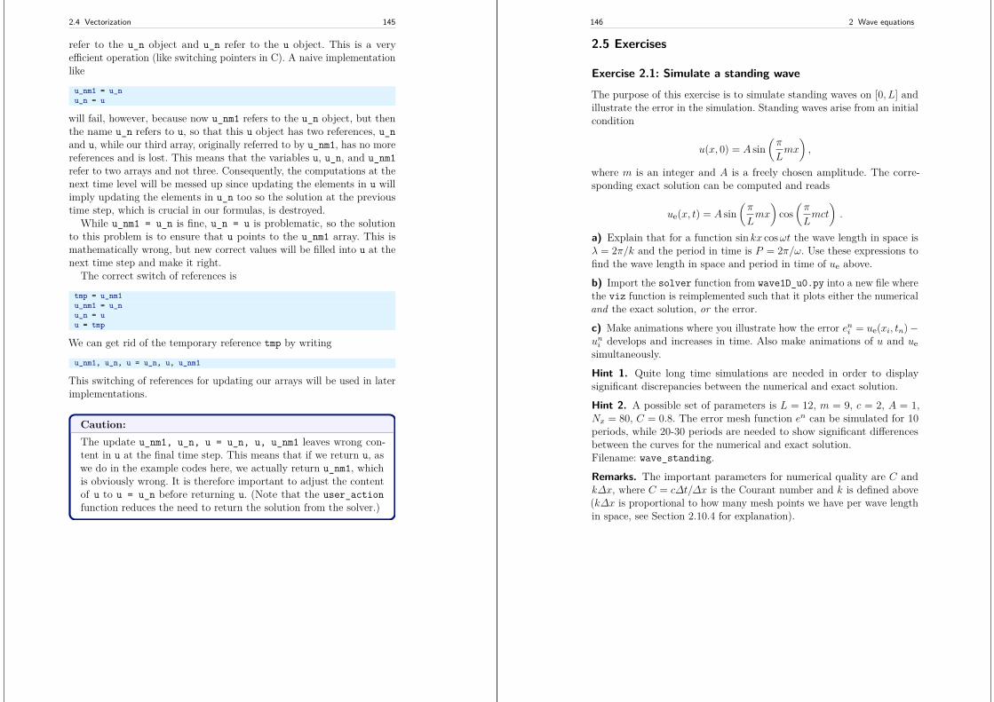
2.4 Vectorization 145
refer to the u_n object and u_n refer to the u object. This is a veryefficient operation (like switching pointers in C). A naive implementationlike
u_nm1 = u_nu_n = u
will fail, however, because now u_nm1 refers to the u_n object, but thenthe name u_n refers to u, so that this u object has two references, u_nand u, while our third array, originally referred to by u_nm1, has no morereferences and is lost. This means that the variables u, u_n, and u_nm1refer to two arrays and not three. Consequently, the computations at thenext time level will be messed up since updating the elements in u willimply updating the elements in u_n too so the solution at the previoustime step, which is crucial in our formulas, is destroyed.
While u_nm1 = u_n is fine, u_n = u is problematic, so the solutionto this problem is to ensure that u points to the u_nm1 array. This ismathematically wrong, but new correct values will be filled into u at thenext time step and make it right.
The correct switch of references is
tmp = u_nm1u_nm1 = u_nu_n = uu = tmp
We can get rid of the temporary reference tmp by writing
u_nm1, u_n, u = u_n, u, u_nm1
This switching of references for updating our arrays will be used in laterimplementations.
Caution:The update u_nm1, u_n, u = u_n, u, u_nm1 leaves wrong con-tent in u at the final time step. This means that if we return u, aswe do in the example codes here, we actually return u_nm1, whichis obviously wrong. It is therefore important to adjust the contentof u to u = u_n before returning u. (Note that the user_actionfunction reduces the need to return the solution from the solver.)
146 2 Wave equations
2.5 Exercises
Exercise 2.1: Simulate a standing wave
The purpose of this exercise is to simulate standing waves on [0, L] andillustrate the error in the simulation. Standing waves arise from an initialcondition
u(x, 0) = A sin(π
Lmx
),
where m is an integer and A is a freely chosen amplitude. The corre-sponding exact solution can be computed and reads
ue(x, t) = A sin(π
Lmx
)cos
(π
Lmct
).
a) Explain that for a function sin kx cosωt the wave length in space isλ = 2π/k and the period in time is P = 2π/ω. Use these expressions tofind the wave length in space and period in time of ue above.
b) Import the solver function from wave1D_u0.py into a new file wherethe viz function is reimplemented such that it plots either the numericaland the exact solution, or the error.
c) Make animations where you illustrate how the error eni = ue(xi, tn)−uni develops and increases in time. Also make animations of u and uesimultaneously.
Hint 1. Quite long time simulations are needed in order to displaysignificant discrepancies between the numerical and exact solution.
Hint 2. A possible set of parameters is L = 12, m = 9, c = 2, A = 1,Nx = 80, C = 0.8. The error mesh function en can be simulated for 10periods, while 20-30 periods are needed to show significant differencesbetween the curves for the numerical and exact solution.Filename: wave_standing.
Remarks. The important parameters for numerical quality are C andk∆x, where C = c∆t/∆x is the Courant number and k is defined above(k∆x is proportional to how many mesh points we have per wave lengthin space, see Section 2.10.4 for explanation).
2.5 Exercises 147
Exercise 2.2: Add storage of solution in a user action functionExtend the plot_u function in the file wave1D_u0.py to also store thesolutions u in a list. To this end, declare all_u as an empty list in theviz function, outside plot_u, and perform an append operation insidethe plot_u function. Note that a function, like plot_u, inside anotherfunction, like viz, remembers all local variables in viz function, includingall_u, even when plot_u is called (as user_action) in the solverfunction. Test both all_u.append(u) and all_u.append(u.copy()).Why does one of these constructions fail to store the solution correctly?Let the viz function return the all_u list converted to a two-dimensionalnumpy array.Filename: wave1D_u0_s_store.
Exercise 2.3: Use a class for the user action functionRedo Exercise 2.2 using a class for the user action function. Let the all_ulist be an attribute in this class and implement the user action functionas a method (the special method __call__ is a natural choice). Theclass versions avoid that the user action function depends on parametersdefined outside the function (such as all_u in Exercise 2.2).Filename: wave1D_u0_s2c.
Exercise 2.4: Compare several Courant numbers in one movieThe goal of this exercise is to make movies where several curves, corre-sponding to different Courant numbers, are visualized. Write a programthat resembles wave1D_u0_s2c.py in Exercise 2.3, but with a viz func-tion that can take a list of C values as argument and create a moviewith solutions corresponding to the given C values. The plot_u functionmust be changed to store the solution in an array (see Exercise 2.2 or 2.3for details), solver must be computed for each value of the Courantnumber, and finally one must run through each time step and plot allthe spatial solution curves in one figure and store it in a file.
The challenge in such a visualization is to ensure that the curves inone plot correspond to the same time point. The easiest remedy is tokeep the time resolution constant and change the space resolution tochange the Courant number. Note that each spatial grid is needed forthe final plotting, so it is an option to store those grids too.Filename: wave_numerics_comparison.
148 2 Wave equations
Exercise 2.5: Implementing the solver function as a generatorThe callback function user_action(u, x, t, n) is called from thesolver function (in, e.g., wave1D_u0.py) at every time level and letsthe user work perform desired actions with the solution, like plotting iton the screen. We have implemented the callback function in the typicalway it would have been done in C and Fortran. Specifically, the codelooks like
if user_action is not None:if user_action(u, x, t, n):
break
Many Python programmers, however, may claim that solver is aniterative process, and that iterative processes with callbacks to the usercode is more elegantly implemented as generators. The rest of the texthas little meaning unless you are familiar with Python generators andthe yield statement.
Instead of calling user_action, the solver function issues a yieldstatement, which is a kind of return statement:
yield u, x, t, n
The program control is directed back to the calling code:
for u, x, t, n in solver(...):# Do something with u at t[n]
When the block is done, solver continues with the statement afteryield. Note that the functionality of terminating the solution process ifuser_action returns a True value is not possible to implement in thegenerator case.
Implement the solver function as a generator, and plot the solutionat each time step. Filename: wave1D_u0_generator.
Project 2.6: Calculus with 1D mesh functionsThis project explores integration and differentiation of mesh functions,both with scalar and vectorized implementations. We are given a meshfunction fi on a spatial one-dimensional mesh xi = i∆x, i = 0, . . . , Nx,over the interval [a, b].a) Define the discrete derivative of fi by using centered differencesat internal mesh points and one-sided differences at the end points.Implement a scalar version of the computation in a Python function and
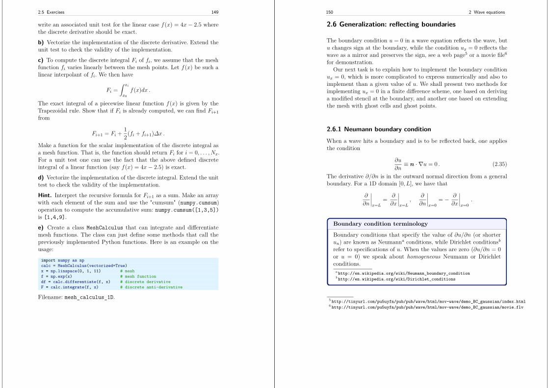
2.5 Exercises 149
write an associated unit test for the linear case f(x) = 4x− 2.5 wherethe discrete derivative should be exact.
b) Vectorize the implementation of the discrete derivative. Extend theunit test to check the validity of the implementation.
c) To compute the discrete integral Fi of fi, we assume that the meshfunction fi varies linearly between the mesh points. Let f(x) be such alinear interpolant of fi. We then have
Fi =∫ xi
x0
f(x)dx .
The exact integral of a piecewise linear function f(x) is given by theTrapezoidal rule. Show that if Fi is already computed, we can find Fi+1from
Fi+1 = Fi + 12(fi + fi+1)∆x .
Make a function for the scalar implementation of the discrete integral asa mesh function. That is, the function should return Fi for i = 0, . . . , Nx.For a unit test one can use the fact that the above defined discreteintegral of a linear function (say f(x) = 4x− 2.5) is exact.
d) Vectorize the implementation of the discrete integral. Extend the unittest to check the validity of the implementation.
Hint. Interpret the recursive formula for Fi+1 as a sum. Make an arraywith each element of the sum and use the "cumsum" (numpy.cumsum)operation to compute the accumulative sum: numpy.cumsum([1,3,5])is [1,4,9].
e) Create a class MeshCalculus that can integrate and differentiatemesh functions. The class can just define some methods that call thepreviously implemented Python functions. Here is an example on theusage:
import numpy as npcalc = MeshCalculus(vectorized=True)x = np.linspace(0, 1, 11) # meshf = np.exp(x) # mesh functiondf = calc.differentiate(f, x) # discrete derivativeF = calc.integrate(f, x) # discrete anti-derivative
Filename: mesh_calculus_1D.
150 2 Wave equations
2.6 Generalization: reflecting boundaries
The boundary condition u = 0 in a wave equation reflects the wave, butu changes sign at the boundary, while the condition ux = 0 reflects thewave as a mirror and preserves the sign, see a web page5 or a movie file6
for demonstration.Our next task is to explain how to implement the boundary condition
ux = 0, which is more complicated to express numerically and also toimplement than a given value of u. We shall present two methods forimplementing ux = 0 in a finite difference scheme, one based on derivinga modified stencil at the boundary, and another one based on extendingthe mesh with ghost cells and ghost points.
2.6.1 Neumann boundary condition
When a wave hits a boundary and is to be reflected back, one appliesthe condition
∂u
∂n≡ n · ∇u = 0 . (2.35)
The derivative ∂/∂n is in the outward normal direction from a generalboundary. For a 1D domain [0, L], we have that
∂
∂n
∣∣∣∣x=L
= ∂
∂x
∣∣∣∣x=L
,∂
∂n
∣∣∣∣x=0
= − ∂
∂x
∣∣∣∣x=0
.
Boundary condition terminology
Boundary conditions that specify the value of ∂u/∂n (or shorterun) are known as Neumanna conditions, while Dirichlet conditionsb
refer to specifications of u. When the values are zero (∂u/∂n = 0or u = 0) we speak about homogeneous Neumann or Dirichletconditions.
a http://en.wikipedia.org/wiki/Neumann_boundary_conditionb http://en.wikipedia.org/wiki/Dirichlet_conditions
5 http://tinyurl.com/pu5uyfn/pub/pub/wave/html/mov-wave/demo_BC_gaussian/index.html6 http://tinyurl.com/pu5uyfn/pub/pub/wave/html/mov-wave/demo_BC_gaussian/movie.flv
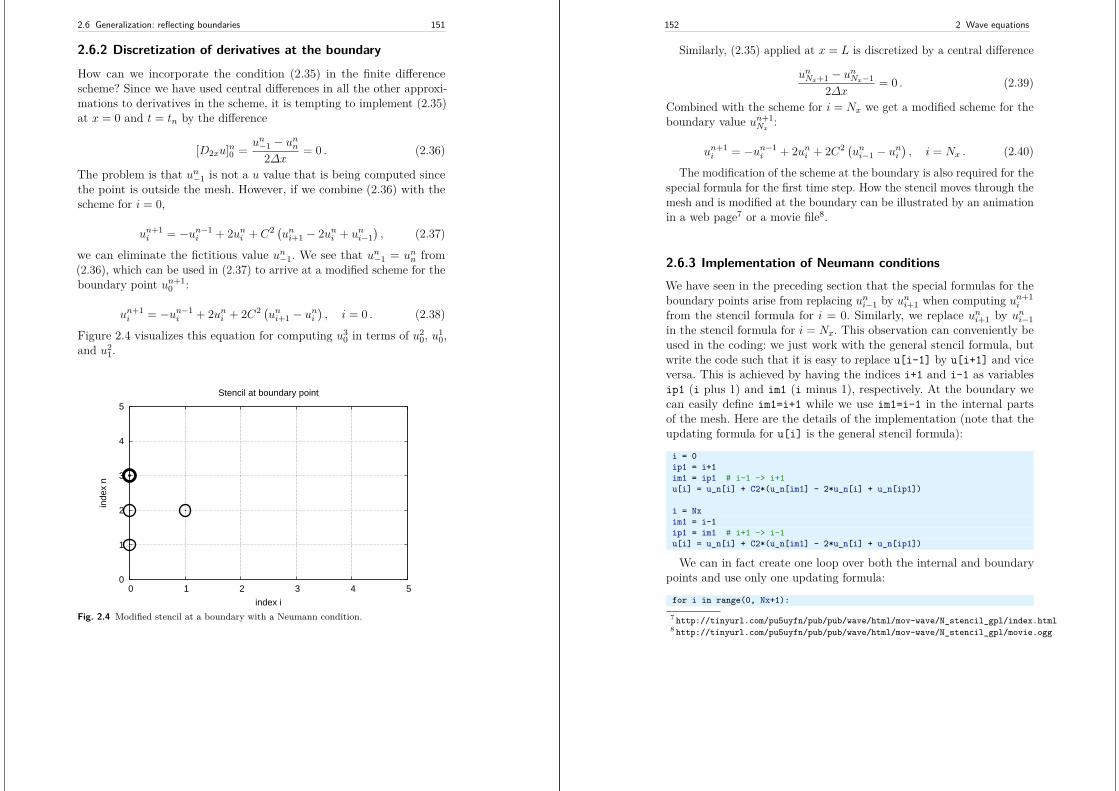
2.6 Generalization: reflecting boundaries 151
2.6.2 Discretization of derivatives at the boundary
How can we incorporate the condition (2.35) in the finite differencescheme? Since we have used central differences in all the other approxi-mations to derivatives in the scheme, it is tempting to implement (2.35)at x = 0 and t = tn by the difference
[D2xu]n0 = un−1 − unn2∆x = 0 . (2.36)
The problem is that un−1 is not a u value that is being computed sincethe point is outside the mesh. However, if we combine (2.36) with thescheme for i = 0,
un+1i = −un−1
i + 2uni + C2 (uni+1 − 2uni + uni−1), (2.37)
we can eliminate the fictitious value un−1. We see that un−1 = unn from(2.36), which can be used in (2.37) to arrive at a modified scheme for theboundary point un+1
0 :
un+1i = −un−1
i + 2uni + 2C2 (uni+1 − uni), i = 0 . (2.38)
Figure 2.4 visualizes this equation for computing u30 in terms of u2
0, u10,
and u21.
0
1
2
3
4
5
0 1 2 3 4 5
inde
x n
index i
Stencil at boundary point
Fig. 2.4 Modified stencil at a boundary with a Neumann condition.
152 2 Wave equations
Similarly, (2.35) applied at x = L is discretized by a central difference
unNx+1 − unNx−12∆x = 0 . (2.39)
Combined with the scheme for i = Nx we get a modified scheme for theboundary value un+1
Nx:
un+1i = −un−1
i + 2uni + 2C2 (uni−1 − uni), i = Nx . (2.40)
The modification of the scheme at the boundary is also required for thespecial formula for the first time step. How the stencil moves through themesh and is modified at the boundary can be illustrated by an animationin a web page7 or a movie file8.
2.6.3 Implementation of Neumann conditionsWe have seen in the preceding section that the special formulas for theboundary points arise from replacing uni−1 by uni+1 when computing un+1
i
from the stencil formula for i = 0. Similarly, we replace uni+1 by uni−1in the stencil formula for i = Nx. This observation can conveniently beused in the coding: we just work with the general stencil formula, butwrite the code such that it is easy to replace u[i-1] by u[i+1] and viceversa. This is achieved by having the indices i+1 and i-1 as variablesip1 (i plus 1) and im1 (i minus 1), respectively. At the boundary wecan easily define im1=i+1 while we use im1=i-1 in the internal partsof the mesh. Here are the details of the implementation (note that theupdating formula for u[i] is the general stencil formula):
i = 0ip1 = i+1im1 = ip1 # i-1 -> i+1u[i] = u_n[i] + C2*(u_n[im1] - 2*u_n[i] + u_n[ip1])
i = Nxim1 = i-1ip1 = im1 # i+1 -> i-1u[i] = u_n[i] + C2*(u_n[im1] - 2*u_n[i] + u_n[ip1])
We can in fact create one loop over both the internal and boundarypoints and use only one updating formula:
for i in range(0, Nx+1):
7 http://tinyurl.com/pu5uyfn/pub/pub/wave/html/mov-wave/N_stencil_gpl/index.html8 http://tinyurl.com/pu5uyfn/pub/pub/wave/html/mov-wave/N_stencil_gpl/movie.ogg
2.6 Generalization: reflecting boundaries 153
ip1 = i+1 if i < Nx else i-1im1 = i-1 if i > 0 else i+1u[i] = u_n[i] + C2*(u_n[im1] - 2*u_n[i] + u_n[ip1])
The program wave1D_n0.py contains a complete implementation ofthe 1D wave equation with boundary conditions ux = 0 at x = 0 andx = L.
It would be nice to modify the test_quadratic test case from thewave1D_u0.py with Dirichlet conditions, described in Section 2.4.3. How-ever, the Neumann conditions require the polynomial variation in thex direction to be of third degree, which causes challenging problemswhen designing a test where the numerical solution is known exactly.Exercise 2.15 outlines ideas and code for this purpose. The only test inwave1D_n0.py is to start with a plug wave at rest and see that the initialcondition is reached again perfectly after one period of motion, but sucha test requires C = 1 (so the numerical solution coincides with the exactsolution of the PDE, see Section 2.10.4).
2.6.4 Index set notation
To improve our mathematical writing and our implementations, it is wiseto introduce a special notation for index sets. This means that we writexi, followed by i ∈ Ix, instead of i = 0, . . . , Nx. Obviously, Ix must bethe index set Ix = 0, . . . , Nx, but it is often advantageous to have asymbol for this set rather than specifying all its elements (all the time,as we have done up to now). This new notation saves writing and makesspecifications of algorithms and their implementation as computer codesimpler.
The first index in the set will be denoted I0x and the last I−1
x . Whenwe need to skip the first element of the set, we use I+
x for the remainingsubset I+
x = 1, . . . , Nx. Similarly, if the last element is to be dropped,we write I−x = 0, . . . , Nx − 1 for the remaining indices. All the indicescorresponding to inner grid points are specified by Iix = 1, . . . , Nx − 1.For the time domain we find it natural to explicitly use 0 as the firstindex, so we will usually write n = 0 and t0 rather than n = I0
t . We alsoavoid notation like xI−1
xand will instead use xi, i = I−1
x .The Python code associated with index sets applies the following
conventions:
154 2 Wave equations
Notation PythonIx IxI0x Ix[0]I−1x Ix[-1]I−x Ix[:-1]I+x Ix[1:]Iix Ix[1:-1]
Why index sets are useful
An important feature of the index set notation is that it keeps ourformulas and code independent of how we count mesh points. Forexample, the notation i ∈ Ix or i = I0
x remains the same whetherIx is defined as above or as starting at 1, i.e., Ix = 1, . . . , Q. Simi-larly, we can in the code define Ix=range(Nx+1) or Ix=range(1,Q),and expressions like Ix[0] and Ix[1:-1] remain correct. One ap-plication where the index set notation is convenient is conversion ofcode from a language where arrays has base index 0 (e.g., Pythonand C) to languages where the base index is 1 (e.g., MATLABand Fortran). Another important application is implementation ofNeumann conditions via ghost points (see next section).
For the current problem setting in the x, t plane, we work with theindex sets
Ix = 0, . . . , Nx, It = 0, . . . , Nt, (2.41)
defined in Python as
Ix = range(0, Nx+1)It = range(0, Nt+1)
A finite difference scheme can with the index set notation be specifiedas
un+1i = uni −
12C
2 (uni+1 − 2uni + uni−1), , i ∈ Iix, n = 0,
un+1i = −un−1
i + 2uni + C2 (uni+1 − 2uni + uni−1), i ∈ Iix, n ∈ Iit ,
un+1i = 0, i = I0
x, n ∈ I−t ,un+1i = 0, i = I−1
x , n ∈ I−t .
2.6 Generalization: reflecting boundaries 155
The corresponding implementation becomes
# Initial conditionfor i in Ix[1:-1]:
u[i] = u_n[i] - 0.5*C2*(u_n[i-1] - 2*u_n[i] + u_n[i+1])
# Time loopfor n in It[1:-1]:
# Compute internal pointsfor i in Ix[1:-1]:
u[i] = - u_nm1[i] + 2*u_n[i] + \C2*(u_n[i-1] - 2*u_n[i] + u_n[i+1])
# Compute boundary conditionsi = Ix[0]; u[i] = 0i = Ix[-1]; u[i] = 0
NoticeThe program wave1D_dn.py applies the index set notation andsolves the 1D wave equation utt = c2uxx + f(x, t) with quite generalboundary and initial conditions:
• x = 0: u = U0(t) or ux = 0• x = L: u = UL(t) or ux = 0• t = 0: u = I(x)• t = 0: ut = V (x)
The program combines Dirichlet and Neumann conditions, scalarand vectorized implementation of schemes, and the index set nota-tion into one piece of code. A lot of test examples are also includedin the program:
• A rectangular plug-shaped initial condition. (For C = 1 thesolution will be a rectangle that jumps one cell per time step,making the case well suited for verification.)
• A Gaussian function as initial condition.• A triangular profile as initial condition, which resembles the
typical initial shape of a guitar string.• A sinusoidal variation of u at x = 0 and either u = 0 or ux = 0
at x = L.• An exact analytical solution u(x, t) = cos(mπt/L) sin(1
2mπx/L),which can be used for convergence rate tests.
156 2 Wave equations
2.6.5 Verifying the implementation of Neumann conditions
How can we test that the Neumann conditions are correctly implemented?The solver function in the wave1D_dn.py program described in the boxabove accepts Dirichlet or Neumann conditions at x = 0 and x = L. Itis tempting to apply a quadratic solution as described in Sections 2.2.1and 2.3.3, but it turns out that this solution is no longer an exact solutionof the discrete equations if a Neumann condition is implemented on theboundary. A linear solution does not help since we only have homogeneousNeumann conditions in wave1D_dn.py, and we are consequently left withtesting just a constant solution: u = const.
def test_constant():"""Check the scalar and vectorized versions fora constant u(x,t). We simulate in [0, L] and applyNeumann and Dirichlet conditions at both ends."""u_const = 0.45u_exact = lambda x, t: u_constI = lambda x: u_exact(x, 0)V = lambda x: 0f = lambda x, t: 0
def assert_no_error(u, x, t, n):u_e = u_exact(x, t[n])diff = np.abs(u - u_e).max()msg = ’diff=%E, t_%d=%g’ % (diff, n, t[n])tol = 1E-13assert diff < tol, msg
for U_0 in (None, lambda t: u_const):for U_L in (None, lambda t: u_const):
L = 2.5c = 1.5C = 0.75Nx = 3 # Very coarse mesh for this exact testdt = C*(L/Nx)/cT = 18 # long time integration
solver(I, V, f, c, U_0, U_L, L, dt, C, T,user_action=assert_no_error,version=’scalar’)
solver(I, V, f, c, U_0, U_L, L, dt, C, T,user_action=assert_no_error,version=’vectorized’)
print U_0, U_L
The quadratic solution is very useful for testing, but it requires Dirichletconditions at both ends.
2.6 Generalization: reflecting boundaries 157
Another test may utilize the fact that the approximation error vanisheswhen the Courant number is unity. We can, for example, start with aplug profile as initial condition, let this wave split into two plug waves,one in each direction, and check that the two plug waves come back andform the initial condition again after “one period” of the solution process.Neumann conditions can be applied at both ends. A proper test functionreads
def test_plug():"""Check that an initial plug is correct back after one period."""L = 1.0c = 0.5dt = (L/10)/c # Nx=10I = lambda x: 0 if abs(x-L/2.0) > 0.1 else 1
u_s, x, t, cpu = solver(I=I,V=None, f=None, c=0.5, U_0=None, U_L=None, L=L,dt=dt, C=1, T=4, user_action=None, version=’scalar’)
u_v, x, t, cpu = solver(I=I,V=None, f=None, c=0.5, U_0=None, U_L=None, L=L,dt=dt, C=1, T=4, user_action=None, version=’vectorized’)
tol = 1E-13diff = abs(u_s - u_v).max()assert diff < tolu_0 = np.array([I(x_) for x_ in x])diff = np.abs(u_s - u_0).max()assert diff < tol
Other tests must rely on an unknown approximation error, so effectivelywe are left with tests on the convergence rate.
2.6.6 Alternative implementation via ghost cells
Idea. Instead of modifying the scheme at the boundary, we can introduceextra points outside the domain such that the fictitious values un−1and unNx+1 are defined in the mesh. Adding the intervals [−∆x, 0] and[L,L + ∆x], known as ghost cells, to the mesh gives us all the neededmesh points, corresponding to i = −1, 0, . . . , Nx, Nx+1. The extra pointswith i = −1 and i = Nx + 1 are known as ghost points, and values atthese points, un−1 and unNx+1, are called ghost values.
The important idea is to ensure that we always have
un−1 = un1 and unNx+1 = unNx−1,
158 2 Wave equations
because then the application of the standard scheme at a boundarypoint i = 0 or i = Nx will be correct and guarantee that the solution iscompatible with the boundary condition ux = 0.
Some readers may find it strange to just extend the domain withghost cells as a general technique, because in some problems there is acompletely different medium with different physics and equations rightoutside of a boundary. Nevertheless, one should view the ghost celltechnique as a purely mathematical technique, which is valid in the limit∆xrightarrow0 and helps us to implement derivatives.Implementation. The u array now needs extra elements correspondingto the ghost points. Two new point values are needed:
u = zeros(Nx+3)
The arrays u_n and u_nm1 must be defined accordingly.Unfortunately, a major indexing problem arises with ghost cells. The
reason is that Python indices must start at 0 and u[-1] will always meanthe last element in u. This fact gives, apparently, a mismatch betweenthe mathematical indices i = −1, 0, . . . , Nx + 1 and the Python indicesrunning over u: 0,..,Nx+2. One remedy is to change the mathematicalindexing of i in the scheme and write
un+1i = · · · , i = 1, . . . , Nx + 1,
instead of i = 0, . . . , Nx as we have previously used. The ghost pointsnow correspond to i = 0 and i = Nx + 1. A better solution is to use theideas of Section 2.6.4: we hide the specific index value in an index set andoperate with inner and boundary points using the index set notation.
To this end, we define u with proper length and Ix to be the corre-sponding indices for the real physical mesh points (1, 2, . . . , Nx + 1):
u = zeros(Nx+3)Ix = range(1, u.shape[0]-1)
That is, the boundary points have indices Ix[0] and Ix[-1] (as before).We first update the solution at all physical mesh points (i.e., interiorpoints in the mesh):
for i in Ix:u[i] = - u_nm1[i] + 2*u_n[i] + \
C2*(u_n[i-1] - 2*u_n[i] + u_n[i+1])
The indexing becomes a bit more complicated when we call functionslike V(x) and f(x, t), as we must remember that the appropriate xcoordinate is given as x[i-Ix[0]]:
2.6 Generalization: reflecting boundaries 159
for i in Ix:u[i] = u_n[i] + dt*V(x[i-Ix[0]]) + \
0.5*C2*(u_n[i-1] - 2*u_n[i] + u_n[i+1]) + \0.5*dt2*f(x[i-Ix[0]], t[0])
It remains to update the solution at ghost points, i.e, u[0] and u[-1](or u[Nx+2]). For a boundary condition ux = 0, the ghost value mustequal the value at the associated inner mesh point. Computer code makesthis statement precise:
i = Ix[0] # x=0 boundaryu[i-1] = u[i+1]i = Ix[-1] # x=L boundaryu[i+1] = u[i-1]
The physical solution to be plotted is now in u[1:-1], or equivalentlyu[Ix[0]:Ix[-1]+1], so this slice is the quantity to be returned froma solver function. A complete implementation appears in the programwave1D_n0_ghost.py.
Warning
We have to be careful with how the spatial and temporal meshpoints are stored. Say we let x be the physical mesh points,
x = linspace(0, L, Nx+1)
"Standard coding" of the initial condition,
for i in Ix:u_n[i] = I(x[i])
becomes wrong, since u_n and x have different lengths and theindex i corresponds to two different mesh points. In fact, x[i]corresponds to u[1+i]. A correct implementation is
for i in Ix:u_n[i] = I(x[i-Ix[0]])
Similarly, a source term usually coded as f(x[i], t[n]) is incorrectif x is defined to be the physical points, so x[i] must be replacedby x[i-Ix[0]].
An alternative remedy is to let x also cover the ghost points suchthat u[i] is the value at x[i].
The ghost cell is only added to the boundary where we have a Neu-mann condition. Suppose we have a Dirichlet condition at x = L and
160 2 Wave equations
a homogeneous Neumann condition at x = 0. One ghost cell [−∆x, 0]is added to the mesh, so the index set for the physical points becomes1, . . . , Nx + 1. A relevant implementation is
u = zeros(Nx+2)Ix = range(1, u.shape[0])...for i in Ix[:-1]:
u[i] = - u_nm1[i] + 2*u_n[i] + \C2*(u_n[i-1] - 2*u_n[i] + u_n[i+1]) + \dt2*f(x[i-Ix[0]], t[n])
i = Ix[-1]u[i] = U_0 # set Dirichlet valuei = Ix[0]u[i-1] = u[i+1] # update ghost value
The physical solution to be plotted is now in u[1:] or (as always)u[Ix[0]:Ix[-1]+1].
2.7 Generalization: variable wave velocity
Our next generalization of the 1D wave equation (2.1) or (2.17) is toallow for a variable wave velocity c: c = c(x), usually motivated by wavemotion in a domain composed of different physical media. When themedia differ in physical properties like density or porosity, the wavevelocity c is affected and will depend on the position in space. Figure 2.5shows a wave propagating in one medium [0, 0.7] ∪ [0.9, 1] with wavevelocity c1 (left) before it enters a second medium (0.7, 0.9) with wavevelocity c2 (right). When the wave passes the boundary where c jumpsfrom c1 to c2, a part of the wave is reflected back into the first medium(the reflected wave), while one part is transmitted through the secondmedium (the transmitted wave).
2.7.1 The model PDE with a variable coefficient
Instead of working with the squared quantity c2(x), we shall for notationalconvenience introduce q(x) = c2(x). A 1D wave equation with variablewave velocity often takes the form
∂2u
∂t2= ∂
∂x
(q(x)∂u
∂x
)+ f(x, t) . (2.42)
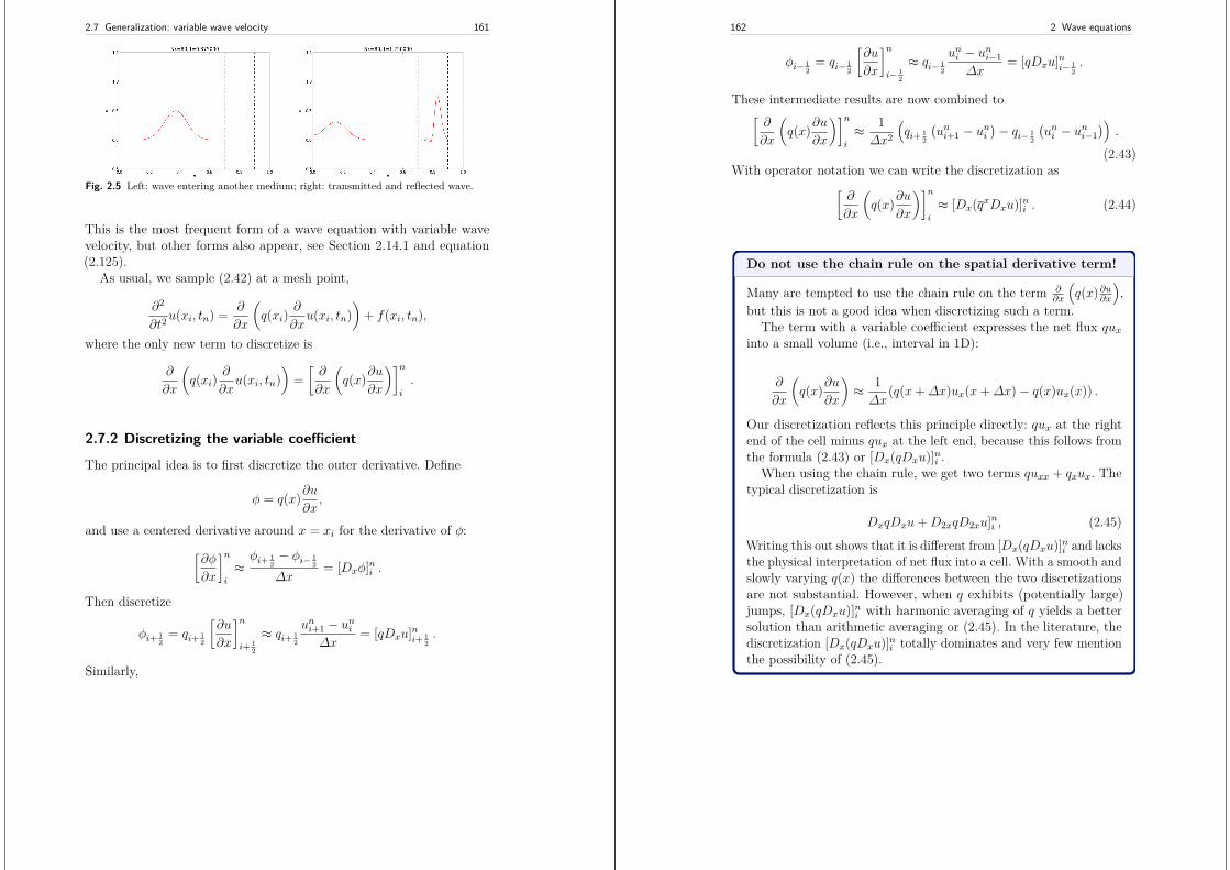
2.7 Generalization: variable wave velocity 161
Fig. 2.5 Left: wave entering another medium; right: transmitted and reflected wave.
This is the most frequent form of a wave equation with variable wavevelocity, but other forms also appear, see Section 2.14.1 and equation(2.125).
As usual, we sample (2.42) at a mesh point,
∂2
∂t2u(xi, tn) = ∂
∂x
(q(xi)
∂
∂xu(xi, tn)
)+ f(xi, tn),
where the only new term to discretize is
∂
∂x
(q(xi)
∂
∂xu(xi, tn)
)=[∂
∂x
(q(x)∂u
∂x
)]n
i
.
2.7.2 Discretizing the variable coefficient
The principal idea is to first discretize the outer derivative. Define
φ = q(x)∂u∂x,
and use a centered derivative around x = xi for the derivative of φ:[∂φ
∂x
]n
i
≈φi+ 1
2− φi− 1
2
∆x= [Dxφ]ni .
Then discretize
φi+ 12
= qi+ 12
[∂u
∂x
]n
i+ 12
≈ qi+ 12
uni+1 − uni∆x
= [qDxu]ni+ 12.
Similarly,
162 2 Wave equations
φi− 12
= qi− 12
[∂u
∂x
]n
i− 12
≈ qi− 12
uni − uni−1∆x
= [qDxu]ni− 12.
These intermediate results are now combined to[∂
∂x
(q(x)∂u
∂x
)]n
i
≈ 1∆x2
(qi+ 1
2
(uni+1 − uni
)− qi− 12
(uni − uni−1
)).
(2.43)With operator notation we can write the discretization as
[∂
∂x
(q(x)∂u
∂x
)]n
i
≈ [Dx(qxDxu)]ni . (2.44)
Do not use the chain rule on the spatial derivative term!
Many are tempted to use the chain rule on the term ∂∂x
(q(x)∂u∂x
),
but this is not a good idea when discretizing such a term.The term with a variable coefficient expresses the net flux qux
into a small volume (i.e., interval in 1D):
∂
∂x
(q(x)∂u
∂x
)≈ 1∆x
(q(x+∆x)ux(x+∆x)− q(x)ux(x)) .
Our discretization reflects this principle directly: qux at the rightend of the cell minus qux at the left end, because this follows fromthe formula (2.43) or [Dx(qDxu)]ni .
When using the chain rule, we get two terms quxx + qxux. Thetypical discretization is
DxqDxu+D2xqD2xu]ni , (2.45)
Writing this out shows that it is different from [Dx(qDxu)]ni and lacksthe physical interpretation of net flux into a cell. With a smooth andslowly varying q(x) the differences between the two discretizationsare not substantial. However, when q exhibits (potentially large)jumps, [Dx(qDxu)]ni with harmonic averaging of q yields a bettersolution than arithmetic averaging or (2.45). In the literature, thediscretization [Dx(qDxu)]ni totally dominates and very few mentionthe possibility of (2.45).
2.7 Generalization: variable wave velocity 163
2.7.3 Computing the coefficient between mesh points
If q is a known function of x, we can easily evaluate qi+ 12simply as
q(xi+ 12) with xi+ 1
2= xi + 1
2∆x. However, in many cases c, and henceq, is only known as a discrete function, often at the mesh points xi.Evaluating q between two mesh points xi and xi+1 must then be doneby interpolation techniques, of which three are of particular interest inthis context:
qi+ 12≈ 1
2 (qi + qi+1) = [qx]i (arithmetic mean) (2.46)
qi+ 12≈ 2
( 1qi
+ 1qi+1
)−1(harmonic mean) (2.47)
qi+ 12≈ (qiqi+1)1/2 (geometric mean) (2.48)
The arithmetic mean in (2.46) is by far the most commonly used averagingtechnique and is well suited for smooth q(x) functions. The harmonicmean is often preferred when q(x) exhibits large jumps (which is typicalfor geological media). The geometric mean is less used, but popular indiscretizations to linearize quadratic nonlinearities (see Section 1.10.2for an example).
With the operator notation from (2.46) we can specify the discretiza-tion of the complete variable-coefficient wave equation in a compactway:
[DtDtu = DxqxDxu+ f ]ni . (2.49)
Strictly speaking, [DxqxDxu]ni = [Dx(qxDxu)]ni .
From the compact difference notation we immediately see what kindof differences that each term is approximated with. The notation qx alsospecifies that the variable coefficient is approximated by an arithmeticmean, the definition being [qx]i+ 1
2= (qi + qi+1)/2.
Before implementing, it remains to solve (2.49) with respect to un+1i :
un+1i = −un−1
i + 2uni +(∆t
∆x
)2 (12(qi + qi+1)(uni+1 − uni )− 1
2(qi + qi−1)(uni − uni−1))
+
∆t2fni . (2.50)
164 2 Wave equations
2.7.4 How a variable coefficient affects the stabilityThe stability criterion derived in Section 2.10.3 reads ∆t ≤ ∆x/c. Ifc = c(x), the criterion will depend on the spatial location. We musttherefore choose a ∆t that is small enough such that no mesh cell has∆x/c(x) > ∆t. That is, we must use the largest c value in the criterion:
∆t ≤ β∆x
maxx∈[0,L] c(x) . (2.51)
The parameter β is included as a safety factor: in some problems with asignificantly varying c it turns out that one must choose β < 1 to havestable solutions (β = 0.9 may act as an all-round value).
A different strategy to handle the stability criterion with variable wavevelocity is to use a spatially varying ∆t. While the idea is mathemati-cally attractive at first sight, the implementation quickly becomes verycomplicated, so we stick to a constant ∆t and a worst case value of c(x)(with a safety factor β).
2.7.5 Neumann condition and a variable coefficientConsider a Neumann condition ∂u/∂x = 0 at x = L = Nx∆x, discretizedas
[D2xu]ni = uni+1 − uni−12∆x = 0 ⇒ uni+1 = uni−1,
for i = Nx. Using the scheme (2.50) at the end point i = Nx withuni+1 = uni−1 results in
un+1i = −un−1
i + 2uni +(∆t
∆x
)2 (qi+ 1
2(uni−1 − uni )− qi− 1
2(uni − uni−1)
)+∆t2fni (2.52)
= −un−1i + 2uni +
(∆t
∆x
)2(qi+ 1
2+ qi− 1
2)(uni−1 − uni ) +∆t2fni
(2.53)
≈ −un−1i + 2uni +
(∆t
∆x
)22qi(uni−1 − uni ) +∆t2fni . (2.54)
Here we used the approximation
2.7 Generalization: variable wave velocity 165
qi+ 12
+ qi− 12
= qi +(dq
dx
)
i
∆x+(d2q
dx2
)
i
∆x2 + · · ·+
qi −(dq
dx
)
i
∆x+(d2q
dx2
)
i
∆x2 + · · ·
= 2qi + 2(d2q
dx2
)
i
∆x2 +O(∆x4)
≈ 2qi . (2.55)
An alternative derivation may apply the arithmetic mean of qn− 12and
qn+ 12in (2.53), leading to the term
(qi + 12(qi+1 + qi−1))(uni−1 − uni ) .
Since 12(qi+1+qi−1) = qi+O(∆x2), we can approximate with 2qi(uni−1−uni )
for i = Nx and get the same term as we did above.A common technique when implementing ∂u/∂x = 0 boundary con-
ditions, is to assume dq/dx = 0 as well. This implies qi+1 = qi−1 andqi+1/2 = qi−1/2 for i = Nx. The implications for the scheme are
un+1i = −un−1
i + 2uni +(∆t
∆x
)2 (qi+ 1
2(uni−1 − uni )− qi− 1
2(uni − uni−1)
)+
∆t2fni (2.56)
= −un−1i + 2uni +
(∆t
∆x
)22qi− 1
2(uni−1 − uni ) +∆t2fni . (2.57)
2.7.6 Implementation of variable coefficients
The implementation of the scheme with a variable wave velocity q(x) =c2(x) may assume that q is available as an array q[i] at the spatial meshpoints. The following loop is a straightforward implementation of thescheme (2.50):
for i in range(1, Nx):u[i] = - u_nm1[i] + 2*u_n[i] + \
C2*(0.5*(q[i] + q[i+1])*(u_n[i+1] - u_n[i]) - \0.5*(q[i] + q[i-1])*(u_n[i] - u_n[i-1])) + \
dt2*f(x[i], t[n])
166 2 Wave equations
The coefficient C2 is now defined as (dt/dx)**2, i.e., not as the squaredCourant number, since the wave velocity is variable and appears insidethe parenthesis.
With Neumann conditions ux = 0 at the boundary, we need to combinethis scheme with the discrete version of the boundary condition, as shownin Section 2.7.5. Nevertheless, it would be convenient to reuse the formulafor the interior points and just modify the indices ip1=i+1 and im1=i-1as we did in Section 2.6.3. Assuming dq/dx = 0 at the boundaries, wecan implement the scheme at the boundary with the following code.
i = 0ip1 = i+1im1 = ip1u[i] = - u_nm1[i] + 2*u_n[i] + \
C2*(0.5*(q[i] + q[ip1])*(u_n[ip1] - u_n[i]) - \0.5*(q[i] + q[im1])*(u_n[i] - u_n[im1])) + \
dt2*f(x[i], t[n])
With ghost cells we can just reuse the formula for the interior pointsalso at the boundary, provided that the ghost values of both u and q arecorrectly updated to ensure ux = 0 and qx = 0.
A vectorized version of the scheme with a variable coefficient at internalmesh points becomes
u[1:-1] = - u_nm1[1:-1] + 2*u_n[1:-1] + \C2*(0.5*(q[1:-1] + q[2:])*(u_n[2:] - u_n[1:-1]) -
0.5*(q[1:-1] + q[:-2])*(u_n[1:-1] - u_n[:-2])) + \dt2*f(x[1:-1], t[n])
2.7.7 A more general PDE model with variable coefficientsSometimes a wave PDE has a variable coefficient in front of the time-derivative term:
%(x)∂2u
∂t2= ∂
∂x
(q(x)∂u
∂x
)+ f(x, t) . (2.58)
One example appears when modeling elastic waves in a rod with varyingdensity, cf. (2.14.1) with %(x).
A natural scheme for (2.58) is
[%DtDtu = DxqxDxu+ f ]ni . (2.59)
We realize that the % coefficient poses no particular difficulty, since %enters the formula just as a simple factor in front of a derivative. There
2.7 Generalization: variable wave velocity 167
is hence no need for any averaging of %. Often, % will be moved to theright-hand side, also without any difficulty:
[DtDtu = %−1DxqxDxu+ f ]ni . (2.60)
2.7.8 Generalization: damping
Waves die out by two mechanisms. In 2D and 3D the energy of the wavespreads out in space, and energy conservation then requires the amplitudeto decrease. This effect is not present in 1D. Damping is another causeof amplitude reduction. For example, the vibrations of a string die outbecause of damping due to air resistance and non-elastic effects in thestring.
The simplest way of including damping is to add a first-order derivativeto the equation (in the same way as friction forces enter a vibratingmechanical system):
∂2u
∂t2+ b
∂u
∂t= c2∂
2u
∂x2 + f(x, t), (2.61)
where b ≥ 0 is a prescribed damping coefficient.A typical discretization of (2.61) in terms of centered differences reads
[DtDtu+ bD2tu = c2DxDxu+ f ]ni . (2.62)
Writing out the equation and solving for the unknown un+1i gives the
scheme
un+1i = (1+1
2b∆t)−1((1
2b∆t−1)un−1i +2uni +C2 (uni+1 − 2uni + uni−1
)+∆t2fni ),(2.63)
for i ∈ Iix and n ≥ 1. New equations must be derived for u1i , and for
boundary points in case of Neumann conditions.The damping is very small in many wave phenomena and thus only
evident for very long time simulations. This makes the standard waveequation without damping relevant for a lot of applications.
168 2 Wave equations
2.8 Building a general 1D wave equation solver
The program wave1D_dn_vc.py is a fairly general code for 1D wavepropagation problems that targets the following initial-boundary valueproblem
utt = (c2(x)ux)x + f(x, t), x ∈ (0, L), t ∈ (0, T ] (2.64)u(x, 0) = I(x), x ∈ [0, L] (2.65)ut(x, 0) = V (t), x ∈ [0, L] (2.66)u(0, t) = U0(t) or ux(0, t) = 0, t ∈ (0, T ] (2.67)u(L, t) = UL(t) or ux(L, t) = 0, t ∈ (0, T ] (2.68)
The only new feature here is the time-dependent Dirichlet conditions.These are trivial to implement:
i = Ix[0] # x=0u[i] = U_0(t[n+1])
i = Ix[-1] # x=Lu[i] = U_L(t[n+1])
The solver function is a natural extension of the simplest solverfunction in the initial wave1D_u0.py program, extended with Neumannboundary conditions (ux = 0), time-varying Dirichlet conditions, as wellas a variable wave velocity. The different code segments needed to makethese extensions have been shown and commented upon in the precedingtext. We refer to the solver function in the wave1D_dn_vc.py file for allthe details. Note in that solver function, however, that the techniqueof “hashing” is used to check whether a certain simulation has been runbefore, or not. This technique is further explained in Section C.2.3.
The vectorization is only applied inside the time loop, not for theinitial condition or the first time steps, since this initial work is negligiblefor long time simulations in 1D problems.
The following sections explain various more advanced programmingtechniques applied in the general 1D wave equation solver.
2.8.1 User action function as a class
A useful feature in the wave1D_dn_vc.py program is the specification ofthe user_action function as a class. This part of the program may need
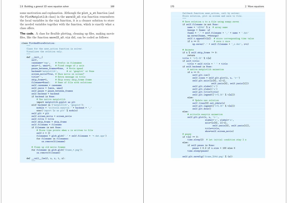
2.8 Building a general 1D wave equation solver 169
some motivation and explanation. Although the plot_u_st function (andthe PlotMatplotlib class) in the wave1D_u0.viz function remembersthe local variables in the viz function, it is a cleaner solution to storethe needed variables together with the function, which is exactly what aclass offers.
The code. A class for flexible plotting, cleaning up files, making moviefiles, like the function wave1D_u0.viz did, can be coded as follows:
class PlotAndStoreSolution:"""Class for the user_action function in solver.Visualizes the solution only."""def __init__(
self,casename=’tmp’, # Prefix in filenamesumin=-1, umax=1, # Fixed range of y axispause_between_frames=None, # Movie speedbackend=’matplotlib’, # or ’gnuplot’ or Nonescreen_movie=True, # Show movie on screen?title=’’, # Extra message in titleskip_frame=1, # Skip every skip_frame framefilename=None): # Name of file with solutionsself.casename = casenameself.yaxis = [umin, umax]self.pause = pause_between_framesself.backend = backendif backend is None:
# Use native matplotlibimport matplotlib.pyplot as plt
elif backend in (’matplotlib’, ’gnuplot’):module = ’scitools.easyviz.’ + backend + ’_’exec(’import %s as plt’ % module)
self.plt = pltself.screen_movie = screen_movieself.title = titleself.skip_frame = skip_frameself.filename = filenameif filename is not None:
# Store time points when u is written to fileself.t = []filenames = glob.glob(’.’ + self.filename + ’*.dat.npz’)for filename in filenames:
os.remove(filename)
# Clean up old movie framesfor filename in glob.glob(’frame_*.png’):
os.remove(filename)
def __call__(self, u, x, t, n):"""
170 2 Wave equations
Callback function user_action, call by solver:Store solution, plot on screen and save to file."""# Save solution u to a file using numpy.savezif self.filename is not None:
name = ’u%04d’ % n # array namekwargs = name: ufname = ’.’ + self.filename + ’_’ + name + ’.dat’np.savez(fname, **kwargs)self.t.append(t[n]) # store corresponding time valueif n == 0: # save x once
np.savez(’.’ + self.filename + ’_x.dat’, x=x)
# Animateif n % self.skip_frame != 0:
returntitle = ’t=%.3f’ % t[n]if self.title:
title = self.title + ’ ’ + titleif self.backend is None:
# native matplotlib animationif n == 0:
self.plt.ion()self.lines = self.plt.plot(x, u, ’r-’)self.plt.axis([x[0], x[-1],
self.yaxis[0], self.yaxis[1]])self.plt.xlabel(’x’)self.plt.ylabel(’u’)self.plt.title(title)self.plt.legend([’t=%.3f’ % t[n]])
else:# Update new solutionself.lines[0].set_ydata(u)self.plt.legend([’t=%.3f’ % t[n]])self.plt.draw()
else:# scitools.easyviz animationself.plt.plot(x, u, ’r-’,
xlabel=’x’, ylabel=’u’,axis=[x[0], x[-1],
self.yaxis[0], self.yaxis[1]],title=title,show=self.screen_movie)
# pauseif t[n] == 0:
time.sleep(2) # let initial condition stay 2 selse:
if self.pause is None:pause = 0.2 if u.size < 100 else 0
time.sleep(pause)
self.plt.savefig(’frame_%04d.png’ % (n))
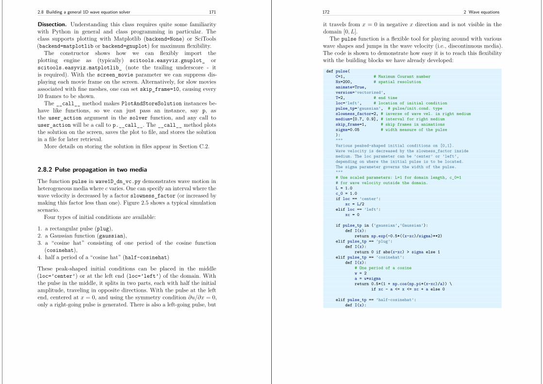
2.8 Building a general 1D wave equation solver 171
Dissection. Understanding this class requires quite some familiaritywith Python in general and class programming in particular. Theclass supports plotting with Matplotlib (backend=None) or SciTools(backend=matplotlib or backend=gnuplot) for maximum flexibility.
The constructor shows how we can flexibly import theplotting engine as (typically) scitools.easyviz.gnuplot_ orscitools.easyviz.matplotlib_ (note the trailing underscore - itis required). With the screen_movie parameter we can suppress dis-playing each movie frame on the screen. Alternatively, for slow moviesassociated with fine meshes, one can set skip_frame=10, causing every10 frames to be shown.
The __call__ method makes PlotAndStoreSolution instances be-have like functions, so we can just pass an instance, say p, asthe user_action argument in the solver function, and any call touser_action will be a call to p.__call__. The __call__ method plotsthe solution on the screen, saves the plot to file, and stores the solutionin a file for later retrieval.
More details on storing the solution in files appear in Section C.2.
2.8.2 Pulse propagation in two media
The function pulse in wave1D_dn_vc.py demonstrates wave motion inheterogeneous media where c varies. One can specify an interval where thewave velocity is decreased by a factor slowness_factor (or increased bymaking this factor less than one). Figure 2.5 shows a typical simulationscenario.
Four types of initial conditions are available:
1. a rectangular pulse (plug),2. a Gaussian function (gaussian),3. a “cosine hat” consisting of one period of the cosine function
(cosinehat),4. half a period of a “cosine hat” (half-cosinehat)
These peak-shaped initial conditions can be placed in the middle(loc=’center’) or at the left end (loc=’left’) of the domain. Withthe pulse in the middle, it splits in two parts, each with half the initialamplitude, traveling in opposite directions. With the pulse at the leftend, centered at x = 0, and using the symmetry condition ∂u/∂x = 0,only a right-going pulse is generated. There is also a left-going pulse, but
172 2 Wave equations
it travels from x = 0 in negative x direction and is not visible in thedomain [0, L].
The pulse function is a flexible tool for playing around with variouswave shapes and jumps in the wave velocity (i.e., discontinuous media).The code is shown to demonstrate how easy it is to reach this flexibilitywith the building blocks we have already developed:
def pulse(C=1, # Maximum Courant numberNx=200, # spatial resolutionanimate=True,version=’vectorized’,T=2, # end timeloc=’left’, # location of initial conditionpulse_tp=’gaussian’, # pulse/init.cond. typeslowness_factor=2, # inverse of wave vel. in right mediummedium=[0.7, 0.9], # interval for right mediumskip_frame=1, # skip frames in animationssigma=0.05 # width measure of the pulse):"""Various peaked-shaped initial conditions on [0,1].Wave velocity is decreased by the slowness_factor insidemedium. The loc parameter can be ’center’ or ’left’,depending on where the initial pulse is to be located.The sigma parameter governs the width of the pulse."""# Use scaled parameters: L=1 for domain length, c_0=1# for wave velocity outside the domain.L = 1.0c_0 = 1.0if loc == ’center’:
xc = L/2elif loc == ’left’:
xc = 0
if pulse_tp in (’gaussian’,’Gaussian’):def I(x):
return np.exp(-0.5*((x-xc)/sigma)**2)elif pulse_tp == ’plug’:
def I(x):return 0 if abs(x-xc) > sigma else 1
elif pulse_tp == ’cosinehat’:def I(x):
# One period of a cosinew = 2a = w*sigmareturn 0.5*(1 + np.cos(np.pi*(x-xc)/a)) \
if xc - a <= x <= xc + a else 0
elif pulse_tp == ’half-cosinehat’:def I(x):
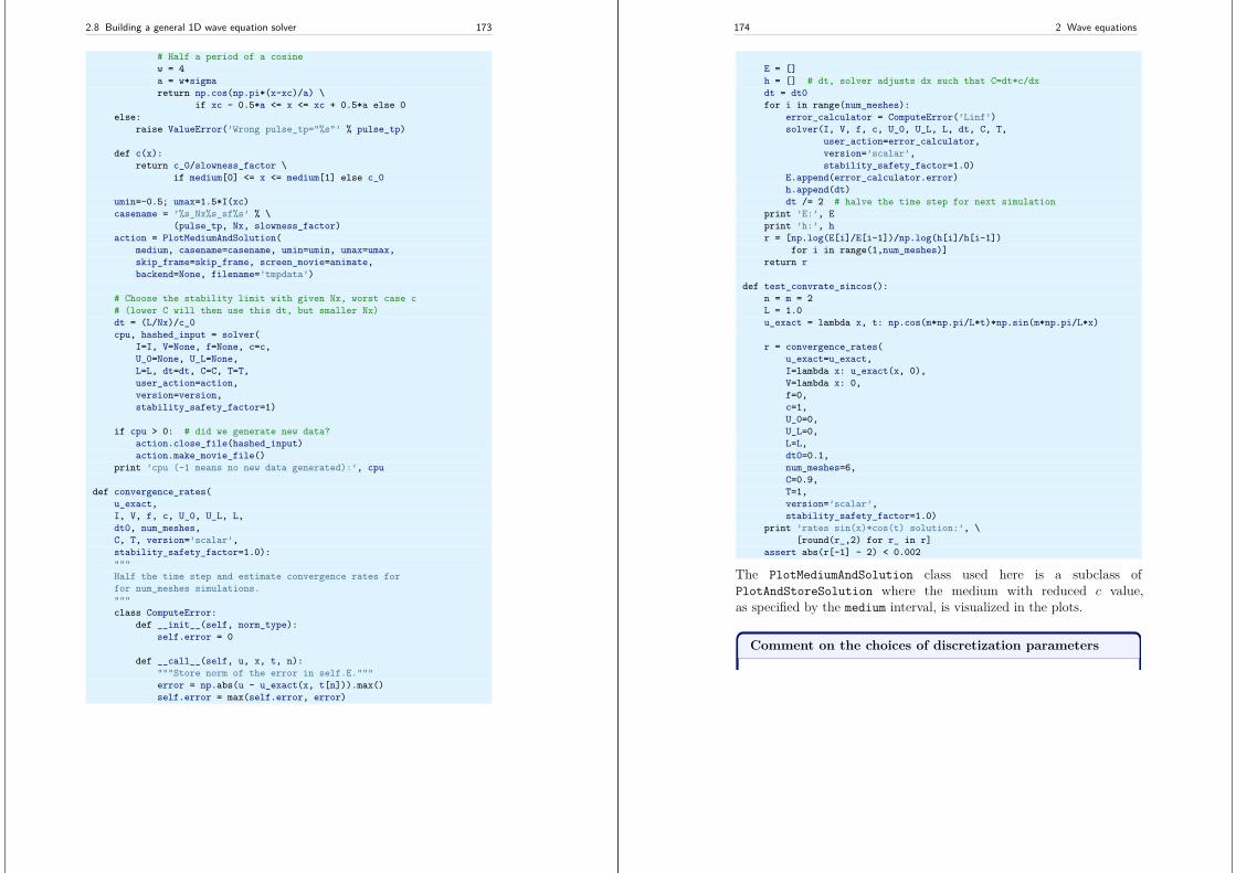
2.8 Building a general 1D wave equation solver 173
# Half a period of a cosinew = 4a = w*sigmareturn np.cos(np.pi*(x-xc)/a) \
if xc - 0.5*a <= x <= xc + 0.5*a else 0else:
raise ValueError(’Wrong pulse_tp="%s"’ % pulse_tp)
def c(x):return c_0/slowness_factor \
if medium[0] <= x <= medium[1] else c_0
umin=-0.5; umax=1.5*I(xc)casename = ’%s_Nx%s_sf%s’ % \
(pulse_tp, Nx, slowness_factor)action = PlotMediumAndSolution(
medium, casename=casename, umin=umin, umax=umax,skip_frame=skip_frame, screen_movie=animate,backend=None, filename=’tmpdata’)
# Choose the stability limit with given Nx, worst case c# (lower C will then use this dt, but smaller Nx)dt = (L/Nx)/c_0cpu, hashed_input = solver(
I=I, V=None, f=None, c=c,U_0=None, U_L=None,L=L, dt=dt, C=C, T=T,user_action=action,version=version,stability_safety_factor=1)
if cpu > 0: # did we generate new data?action.close_file(hashed_input)action.make_movie_file()
print ’cpu (-1 means no new data generated):’, cpu
def convergence_rates(u_exact,I, V, f, c, U_0, U_L, L,dt0, num_meshes,C, T, version=’scalar’,stability_safety_factor=1.0):"""Half the time step and estimate convergence rates forfor num_meshes simulations."""class ComputeError:
def __init__(self, norm_type):self.error = 0
def __call__(self, u, x, t, n):"""Store norm of the error in self.E."""error = np.abs(u - u_exact(x, t[n])).max()self.error = max(self.error, error)
174 2 Wave equations
E = []h = [] # dt, solver adjusts dx such that C=dt*c/dxdt = dt0for i in range(num_meshes):
error_calculator = ComputeError(’Linf’)solver(I, V, f, c, U_0, U_L, L, dt, C, T,
user_action=error_calculator,version=’scalar’,stability_safety_factor=1.0)
E.append(error_calculator.error)h.append(dt)dt /= 2 # halve the time step for next simulation
print ’E:’, Eprint ’h:’, hr = [np.log(E[i]/E[i-1])/np.log(h[i]/h[i-1])
for i in range(1,num_meshes)]return r
def test_convrate_sincos():n = m = 2L = 1.0u_exact = lambda x, t: np.cos(m*np.pi/L*t)*np.sin(m*np.pi/L*x)
r = convergence_rates(u_exact=u_exact,I=lambda x: u_exact(x, 0),V=lambda x: 0,f=0,c=1,U_0=0,U_L=0,L=L,dt0=0.1,num_meshes=6,C=0.9,T=1,version=’scalar’,stability_safety_factor=1.0)
print ’rates sin(x)*cos(t) solution:’, \[round(r_,2) for r_ in r]
assert abs(r[-1] - 2) < 0.002
The PlotMediumAndSolution class used here is a subclass ofPlotAndStoreSolution where the medium with reduced c value,as specified by the medium interval, is visualized in the plots.
Comment on the choices of discretization parameters
2.9 Exercises 175
The argument Nx in the pulse function does not correspond tothe actual spatial resolution of C < 1, since the solver functiontakes a fixed ∆t and C, and adjusts ∆x accordingly. As seen in thepulse function, the specified ∆t is chosen according to the limitC = 1, so if C < 1, ∆t remains the same, but the solver functionoperates with a larger ∆x and smaller Nx than was specified in thecall to pulse. The practical reason is that we always want to keep∆t fixed such that plot frames and movies are synchronized in timeregardless of the value of C (i.e., ∆x is varied when the Courantnumber varies).
The reader is encouraged to play around with the pulse function:
>>> import wave1D_dn_vc as w>>> w.pulse(Nx=50, loc=’left’, pulse_tp=’cosinehat’, slowness_factor=2)
To easily kill the graphics by Ctrl-C and restart a new simulation itmight be easier to run the above two statements from the command linewith
Terminal
Terminal> python -c ’import wave1D_dn_vc as w; w.pulse(...)’
2.9 Exercises
Exercise 2.7: Find the analytical solution to a damped waveequation
Consider the wave equation with damping (2.61). The goal is to find anexact solution to a wave problem with damping and zero source term. Astarting point is the standing wave solution from Exercise 2.1. It becomesnecessary to include a damping term e−βt and also have both a sine andcosine component in time:
ue(x, t) = e−βt sin kx (A cosωt+B sinωt) .
Find k from the boundary conditions u(0, t) = u(L, t) = 0. Then usethe PDE to find constraints on β, ω, A, and B. Set up a completeinitial-boundary value problem and its solution.Filename: damped_waves.
176 2 Wave equations
Problem 2.8: Explore symmetry boundary conditions
Consider the simple "plug" wave where Ω = [−L,L] and
I(x) =
1, x ∈ [−δ, δ],0, otherwise
for some number 0 < δ < L. The other initial condition is ut(x, 0) = 0and there is no source term f . The boundary conditions can be set tou = 0. The solution to this problem is symmetric around x = 0. Thismeans that we can simulate the wave process in only the half of thedomain [0, L].
a) Argue why the symmetry boundary condition is ux = 0 at x = 0.
Hint. Symmetry of a function about x = x0 means that f(x0 + h) =f(x0 − h).
b) Perform simulations of the complete wave problem on [−L,L]. There-after, utilize the symmetry of the solution and run a simulation in half ofthe domain [0, L], using a boundary condition at x = 0. Compare plotsfrom the two solutions and confirm that they are the same.
c) Prove the symmetry property of the solution by setting up thecomplete initial-boundary value problem and showing that if u(x, t) is asolution, then also u(−x, t) is a solution.
d) If the code works correctly, the solution u(x, t) = x(L − x)(1 + t2)
should be reproduced exactly. Write a test function test_quadraticthat checks whether this is the case. Simulate for x in [0, L2 ] with asymmetry condition at the end x = L
2 .Filename: wave1D_symmetric.
Exercise 2.9: Send pulse waves through a layered medium
Use the pulse function in wave1D_dn_vc.py to investigate sending apulse, located with its peak at x = 0, through two media with differentwave velocities. The (scaled) velocity in the left medium is 1 while it is1sf
in the right medium. Report what happens with a Gaussian pulse,a “cosine hat” pulse, half a “cosine hat” pulse, and a plug pulse forresolutions Nx = 40, 80, 160, and sf = 2, 4. Simulate until T = 2.Filename: pulse1D.
2.9 Exercises 177
Exercise 2.10: Explain why numerical noise occurs
The experiments performed in Exercise 2.9 shows considerable numericalnoise in the form of non-physical waves, especially for sf = 4 andthe plug pulse or the half a “cosinehat” pulse. The noise is much lessvisible for a Gaussian pulse. Run the case with the plug and half a“cosinehat” pulses for sf = 1, C = 0.9, 0.25, and Nx = 40, 80, 160. Usethe numerical dispersion relation to explain the observations. Filename:pulse1D_analysis.
Exercise 2.11: Investigate harmonic averaging in a 1D model
Harmonic means are often used if the wave velocity is non-smoothor discontinuous. Will harmonic averaging of the wave velocity giveless numerical noise for the case sf = 4 in Exercise 2.9? Filename:pulse1D_harmonic.
Problem 2.12: Implement open boundary conditions
To enable a wave to leave the computational domain and travel undis-turbed through the boundary x = L, one can in a one-dimensionalproblem impose the following condition, called a radiation condition oropen boundary condition:
∂u
∂t+ c
∂u
∂x= 0 . (2.69)
The parameter c is the wave velocity.Show that (2.69) accepts a solution u = gR(x− ct) (right-going wave),
but not u = gL(x + ct) (left-going wave). This means that (2.69) willallow any right-going wave gR(x − ct) to pass through the boundaryundisturbed.
A corresponding open boundary condition for a left-going wave throughx = 0 is
∂u
∂t− c∂u
∂x= 0 . (2.70)
a) A natural idea for discretizing the condition (2.69) at the spatial endpoint i = Nx is to apply centered differences in time and space:
178 2 Wave equations
[D2tu+ cD2xu = 0]ni , i = Nx . (2.71)
Eliminate the fictitious value unNx+1 by using the discrete equation at thesame point.
The equation for the first step, u1i , is in principle also affected, but we
can then use the condition uNx = 0 since the wave has not yet reachedthe right boundary.b) A much more convenient implementation of the open boundarycondition at x = L can be based on an explicit discretization
[D+t u+ cD−x u = 0]ni , i = Nx . (2.72)
From this equation, one can solve for un+1Nx
and apply the formula as aDirichlet condition at the boundary point. However, the finite differenceapproximations involved are of first order.
Implement this scheme for a wave equation utt = c2uxx in a domain[0, L], where you have ux = 0 at x = 0, the condition (2.69) at x = L,and an initial disturbance in the middle of the domain, e.g., a plug profilelike
u(x, 0) =
1, L/2− ` ≤ x ≤ L/2 + `,0, otherwise
Observe that the initial wave is split in two, the left-going wave is reflectedat x = 0, and both waves travel out of x = L, leaving the solution asu = 0 in [0, L]. Use a unit Courant number such that the numericalsolution is exact. Make a movie to illustrate what happens.
Because this simplified implementation of the open boundary conditionworks, there is no need to pursue the more complicated discretization ina).Hint. Modify the solver function in wave1D_dn.py.c) Add the possibility to have either ux = 0 or an open boundarycondition at the left boundary. The latter condition is discretized as
[D+t u− cD+
x u = 0]ni , i = 0, (2.73)
leading to an explicit update of the boundary value un+10 .
The implementation can be tested with a Gaussian function as initialcondition:
g(x;m, s) = 1√2πs
e−(x−m)2
2s2 .
2.9 Exercises 179
Run two tests:
1. Disturbance in the middle of the domain, I(x) = g(x;L/2, s), andopen boundary condition at the left end.
2. Disturbance at the left end, I(x) = g(x; 0, s), and ux = 0 as symmetryboundary condition at this end.
Make test functions for both cases, testing that the solution is zero afterthe waves have left the domain.
d) In 2D and 3D it is difficult to compute the correct wave velocitynormal to the boundary, which is needed in generalizations of the openboundary conditions in higher dimensions. Test the effect of having aslightly wrong wave velocity in (2.72). Make movies to illustrate whathappens.Filename: wave1D_open_BC.
Remarks. The condition (2.69) works perfectly in 1D when c is known.In 2D and 3D, however, the condition reads ut + cxux + cyuy = 0, wherecx and cy are the wave speeds in the x and y directions. Estimating thesecomponents (i.e., the direction of the wave) is often challenging. Othermethods are normally used in 2D and 3D to let waves move out of acomputational domain.
Exercise 2.13: Implement periodic boundary conditions
It is frequently of interest to follow wave motion over large distancesand long times. A straightforward approach is to work with a very largedomain, but that might lead to a lot of computations in areas of thedomain where the waves cannot be noticed. A more efficient approach isto let a right-going wave out of the domain and at the same time let itenter the domain on the left. This is called a periodic boundary condition.
The boundary condition at the right end x = L is an open boundarycondition (see Exercise 2.12) to let a right-going wave out of the domain.At the left end, x = 0, we apply, in the beginning of the simulation,either a symmetry boundary condition (see Exercise 2.8) ux = 0, or anopen boundary condition.
This initial wave will split in two and either be reflected or transportedout of the domain at x = 0. The purpose of the exercise is to follow theright-going wave. We can do that with a periodic boundary condition.This means that when the right-going wave hits the boundary x = L, the
180 2 Wave equations
open boundary condition lets the wave out of the domain, but at the sametime we use a boundary condition on the left end x = 0 that feeds theoutgoing wave into the domain again. This periodic condition is simplyu(0) = u(L). The switch from ux = 0 or an open boundary conditionat the left end to a periodic condition can happen when u(L, t) > ε,where ε = 10−4 might be an appropriate value for determining when theright-going wave hits the boundary x = L.
The open boundary conditions can conveniently be discretized asexplained in Exercise 2.12. Implement the described type of boundaryconditions and test them on two different initial shapes: a plug u(x, 0) = 1for x ≤ 0.1, u(x, 0) = 0 for x > 0.1, and a Gaussian function in themiddle of the domain: u(x, 0) = exp (−1
2(x− 0.5)2/0.05). The domainis the unit interval [0, 1]. Run these two shapes for Courant numbers 1and 0.5. Assume constant wave velocity. Make movies of the four cases.Reason why the solutions are correct. Filename: periodic.
Exercise 2.14: Compare discretizations of a Neumanncondition
We have a 1D wave equation with variable wave velocity: utt = (qux)x. ANeumann condition ux at x = 0, L can be discretized as shown in (2.54)and (2.57).
The aim of this exercise is to examine the rate of the numerical errorwhen using different ways of discretizing the Neumann condition.
a) As a test problem, q = 1+(x−L/2)4 can be used, with f(x, t) adaptedsuch that the solution has a simple form, say u(x, t) = cos(πx/L) cos(ωt)for, e.g., ω = 1. Perform numerical experiments and find the convergencerate of the error using the approximation (2.54).
b) Switch to q(x) = 1 + cos(πx/L), which is symmetric at x = 0, L,and check the convergence rate of the scheme (2.57). Now, qi−1/2 is a2nd-order approximation to qi, qi−1/2 = qi + 0.25q′′i∆x2 + · · · , becauseq′i = 0 for i = Nx (a similar argument can be applied to the case i = 0).
c) A third discretization can be based on a simple and convenient, but lessaccurate, one-sided difference: ui− ui−1 = 0 at i = Nx and ui+1− ui = 0at i = 0. Derive the resulting scheme in detail and implement it. Runexperiments with q from a) or b) to establish the rate of convergence ofthe scheme.
2.9 Exercises 181
d) A fourth technique is to view the scheme as
[DtDtu]ni = 1∆x
([qDxu]ni+ 1
2− [qDxu]ni− 1
2
)+ [f ]ni ,
and place the boundary at xi+ 12, i = Nx, instead of exactly at the physical
boundary. With this idea of approximating (moving) the boundary, wecan just set [qDxu]n
i+ 12
= 0. Derive the complete scheme using thistechnique. The implementation of the boundary condition at L−∆x/2is O(∆x2) accurate, but the interesting question is what impact themovement of the boundary has on the convergence rate. Compute theerrors as usual over the entire mesh and use q from a) or b).Filename: Neumann_discr.
Exercise 2.15: Verification by a cubic polynomial in space
The purpose of this exercise is to verify the implementation of the solverfunction in the program wave1D_n0.py by using an exact numericalsolution for the wave equation utt = c2uxx + f with Neumann boundaryconditions ux(0, t) = ux(L, t) = 0.
A similar verification is used in the file wave1D_u0.py, which solves thesame PDE, but with Dirichlet boundary conditions u(0, t) = u(L, t) =0. The idea of the verification test in function test_quadratic inwave1D_u0.py is to produce a solution that is a lower-order polyno-mial such that both the PDE problem, the boundary conditions, andall the discrete equations are exactly fulfilled. Then the solver functionshould reproduce this exact solution to machine precision. More precisely,we seek u = X(x)T (t), with T (t) as a linear function and X(x) as aparabola that fulfills the boundary conditions. Inserting this u in thePDE determines f . It turns out that u also fulfills the discrete equations,because the truncation error of the discretized PDE has derivatives in xand t of order four and higher. These derivatives all vanish for a quadraticX(x) and linear T (t).
It would be attractive to use a similar approach in the case of Neumannconditions. We set u = X(x)T (t) and seek lower-order polynomials Xand T . To force ux to vanish at the boundary, we let Xx be a parabola.Then X is a cubic polynomial. The fourth-order derivative of a cubicpolynomial vanishes, so u = X(x)T (t) will fulfill the discretized PDEalso in this case, if f is adjusted such that u fulfills the PDE.
182 2 Wave equations
However, the discrete boundary condition is not exactly fulfilled bythis choice of u. The reason is that
[D2xu]ni = ux(xi, tn) + 16uxxx(xi, tn)∆x2 +O(∆x4) . (2.74)
At the boundary two boundary points, we must demand that the deriva-tive Xx(x) = 0 such that ux = 0. However, uxxx is a constant and notzero when X(x) is a cubic polynomial. Therefore, our u = X(x)T (t)fulfills
[D2xu]ni = 16uxxx(xi, tn)∆x2,
and not
[D2xu]ni = 0, i = 0, Nx,
as it should. (Note that all the higher-order terms O(∆x4) also havehigher-order derivatives that vanish for a cubic polynomial.) So to sum-marize, the fundamental problem is that u as a product of a cubicpolynomial and a linear or quadratic polynomial in time is not an exactsolution of the discrete boundary conditions.
To make progress, we assume that u = X(x)T (t), where T for simplic-ity is taken as a prescribed linear function 1 + 1
2 t, and X(x) is taken asan unknown cubic polynomial
∑3j=0 ajx
j . There are two different waysof determining the coefficients a0, . . . , a3 such that both the discretizedPDE and the discretized boundary conditions are fulfilled, under theconstraint that we can specify a function f(x, t) for the PDE to feed tothe solver function in wave1D_n0.py. Both approaches are explainedin the subexercises.a) One can insert u in the discretized PDE and find the corresponding f .Then one can insert u in the discretized boundary conditions. This yieldstwo equations for the four coefficients a0, . . . , a3. To find the coefficients,one can set a0 = 0 and a1 = 1 for simplicity and then determine a2 anda3. This approach will make a2 and a3 depend on ∆x and f will dependon both ∆x and ∆t.
Use sympy to perform analytical computations. A starting point is todefine u as follows:
def test_cubic1():import sympy as smx, t, c, L, dx, dt = sm.symbols(’x t c L dx dt’)
2.9 Exercises 183
i, n = sm.symbols(’i n’, integer=True)
# Assume discrete solution is a polynomial of degree 3 in xT = lambda t: 1 + sm.Rational(1,2)*t # Temporal terma = sm.symbols(’a_0 a_1 a_2 a_3’)X = lambda x: sum(a[q]*x**q for q in range(4)) # Spatial termu = lambda x, t: X(x)*T(t)
The symbolic expression for u is reached by calling u(x,t) with x and tas sympy symbols.
Define DxDx(u, i, n), DtDt(u, i, n), and D2x(u, i, n) asPython functions for returning the difference approximations [DxDxu]ni ,[DtDtu]ni , and [D2xu]ni . The next step is to set up the residuals for theequations [D2xu]n0 = 0 and [D2xu]nNx = 0, where Nx = L/∆x. Call theresiduals R_0 and R_L. Substitute a0 and a1 by 0 and 1, respectively, inR_0, R_L, and a:
R_0 = R_0.subs(a[0], 0).subs(a[1], 1)R_L = R_L.subs(a[0], 0).subs(a[1], 1)a = list(a) # enable in-place assignmenta[0:2] = 0, 1
Determining a2 and a3 from the discretized boundary conditions is thenabout solving two equations with respect to a2 and a3, i.e., a[2:]:
s = sm.solve([R_0, R_L], a[2:])# s is dictionary with the unknowns a[2] and a[3] as keysa[2:] = s[a[2]], s[a[3]]
Now, a contains computed values and u will automatically use these newvalues since X accesses a.
Compute the source term f from the discretized PDE: fni = [DtDtu−c2DxDxu]ni . Turn u, the time derivative ut (needed for the initial conditionV (x)), and f into Python functions. Set numerical values for L, Nx, C,and c. Prescribe the time interval as ∆t = CL/(Nxc), which imply∆x = c∆t/C = L/Nx. Define new functions I(x), V(x), and f(x,t)as wrappers of the ones made above, where fixed values of L, c, ∆x,and ∆t are inserted, such that I, V, and f can be passed on to thesolver function. Finally, call solver with a user_action function thatcompares the numerical solution to this exact solution u of the discretePDE problem.
Hint. To turn a sympy expression e, depending on a series of sym-bols, say x, t, dx, dt, L, and c, into a plain Python functione_exact(x,t,L,dx,dt,c), one can write
e_exact = sm.lambdify([x,t,L,dx,dt,c], e, ’numpy’)
184 2 Wave equations
The ’numpy’ argument is a good habit as the e_exact function willthen work with array arguments if it contains mathematical functions(but here we only do plain arithmetics, which automatically work witharrays).
b) An alternative way of determining a0, . . . , a3 is to reason as follows.We first construct X(x) such that the boundary conditions are fulfilled:X = x(L− x). However, to compensate for the fact that this choice ofX does not fulfill the discrete boundary condition, we seek u such that
ux = ∂
∂xx(L− x)T (t)− 1
6uxxx∆x2,
since this u will fit the discrete boundary condition. Assuming u =T (t)
∑3j=0 ajx
j , we can use the above equation to determine the coeffi-cients a1, a2, a3. A value, e.g., 1 can be used for a0. The following sympycode computes this u:
def test_cubic2():import sympy as smx, t, c, L, dx = sm.symbols(’x t c L dx’)T = lambda t: 1 + sm.Rational(1,2)*t # Temporal term# Set u as a 3rd-degree polynomial in spaceX = lambda x: sum(a[i]*x**i for i in range(4))a = sm.symbols(’a_0 a_1 a_2 a_3’)u = lambda x, t: X(x)*T(t)# Force discrete boundary condition to be zero by adding# a correction term the analytical suggestion x*(L-x)*T# u_x = x*(L-x)*T(t) - 1/6*u_xxx*dx**2R = sm.diff(u(x,t), x) - (
x*(L-x) - sm.Rational(1,6)*sm.diff(u(x,t), x, x, x)*dx**2)# R is a polynomial: force all coefficients to vanish.# Turn R to Poly to extract coefficients:R = sm.poly(R, x)coeff = R.all_coeffs()s = sm.solve(coeff, a[1:]) # a[0] is not present in R# s is dictionary with a[i] as keys# Fix a[0] as 1s[a[0]] = 1X = lambda x: sm.simplify(sum(s[a[i]]*x**i for i in range(4)))u = lambda x, t: X(x)*T(t)print ’u:’, u(x,t)
The next step is to find the source term f_e by inserting u_e in thePDE. Thereafter, turn u, f, and the time derivative of u into plain Pythonfunctions as in a), and then wrap these functions in new functions I,V, and f, with the right signature as required by the solver function.Set parameters as in a) and check that the solution is exact to machineprecision at each time level using an appropriate user_action function.
2.10 Analysis of the difference equations 185
Filename: wave1D_n0_test_cubic.
2.10 Analysis of the difference equations
2.10.1 Properties of the solution of the wave equation
The wave equation
∂2u
∂t2= c2∂
2u
∂x2
has solutions of the form
u(x, t) = gR(x− ct) + gL(x+ ct), (2.75)
for any functions gR and gL sufficiently smooth to be differentiated twice.The result follows from inserting (2.75) in the wave equation. A functionof the form gR(x − ct) represents a signal moving to the right in timewith constant velocity c. This feature can be explained as follows. Attime t = 0 the signal looks like gR(x). Introducing a moving horizontalcoordinate ξ = x − ct, we see the function gR(ξ) is “at rest” in the ξcoordinate system, and the shape is always the same. Say the gR(ξ)function has a peak at ξ = 0. This peak is located at x = ct, which meansthat it moves with the velocity dx/dt = c in the x coordinate system.Similarly, gL(x+ ct) is a function, initially with shape gL(x), that movesin the negative x direction with constant velocity c (introduce ξ = x+ ct,look at the point ξ = 0, x = −ct, which has velocity dx/dt = −c).
With the particular initial conditions
u(x, 0) = I(x), ∂
∂tu(x, 0) = 0,
we get, with u as in (2.75),
gR(x) + gL(x) = I(x), −cg′R(x) + cg′L(x) = 0 .
The former suggests gR = gL, and the former then leads to gR = gL = I/2.Consequently,
u(x, t) = 12I(x− ct) + 1
2I(x+ ct) . (2.76)
186 2 Wave equations
The interpretation of (2.76) is that the initial shape of u is split into twoparts, each with the same shape as I but half of the initial amplitude.One part is traveling to the left and the other one to the right.
The solution has two important physical features: constant amplitudeof the left and right wave, and constant velocity of these two waves. Itturns out that the numerical solution will also preserve the constantamplitude, but the velocity depends on the mesh parameters ∆t and ∆x.
The solution (2.76) will be influenced by boundary conditions whenthe parts 1
2I(x − ct) and 12I(x + ct) hit the boundaries and get, e.g.,
reflected back into the domain. However, when I(x) is nonzero only in asmall part in the middle of the spatial domain [0, L], which means thatthe boundaries are placed far away from the initial disturbance of u, thesolution (2.76) is very clearly observed in a simulation.
A useful representation of solutions of wave equations is a linearcombination of sine and/or cosine waves. Such a sum of waves is asolution if the governing PDE is linear and each sine or cosine wavefulfills the equation. To ease analytical calculations by hand we shallwork with complex exponential functions instead of real-valued sine orcosine functions. The real part of complex expressions will typically betaken as the physical relevant quantity (whenever a physical relevantquantity is strictly needed). The idea now is to build I(x) of complexwave components eikx:
I(x) ≈∑
k∈Kbke
ikx . (2.77)
Here, k is the frequency of a component, K is some set of all the discretek values needed to approximate I(x) well, and bk are constants that mustbe determined. We will very seldom need to compute the bk coefficients:most of the insight we look for, and the understanding of the numericalmethods we want to establish, come from investigating how the PDEand the scheme treat a single component eikx wave.
Letting the number of k values in K tend to infinity, makes thesum (2.77) converge to I(x). This sum is known as a Fourier seriesrepresentation of I(x). Looking at (2.76), we see that the solution u(x, t),when I(x) is represented as in (2.77), is also built of basic complexexponential wave components of the form eik(x±ct) according to
u(x, t) = 12∑
k∈Kbke
ik(x−ct) + 12∑
k∈Kbke
ik(x+ct) . (2.78)
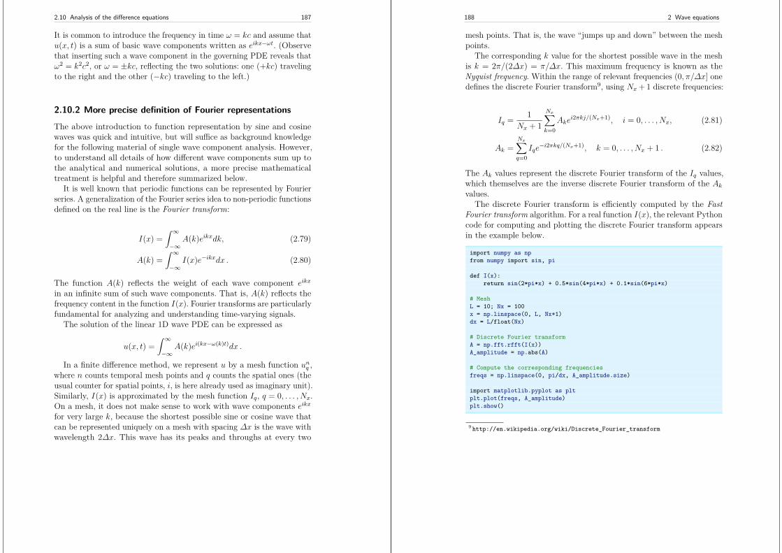
2.10 Analysis of the difference equations 187
It is common to introduce the frequency in time ω = kc and assume thatu(x, t) is a sum of basic wave components written as eikx−ωt. (Observethat inserting such a wave component in the governing PDE reveals thatω2 = k2c2, or ω = ±kc, reflecting the two solutions: one (+kc) travelingto the right and the other (−kc) traveling to the left.)
2.10.2 More precise definition of Fourier representations
The above introduction to function representation by sine and cosinewaves was quick and intuitive, but will suffice as background knowledgefor the following material of single wave component analysis. However,to understand all details of how different wave components sum up tothe analytical and numerical solutions, a more precise mathematicaltreatment is helpful and therefore summarized below.
It is well known that periodic functions can be represented by Fourierseries. A generalization of the Fourier series idea to non-periodic functionsdefined on the real line is the Fourier transform:
I(x) =∫ ∞
−∞A(k)eikxdk, (2.79)
A(k) =∫ ∞
−∞I(x)e−ikxdx . (2.80)
The function A(k) reflects the weight of each wave component eikxin an infinite sum of such wave components. That is, A(k) reflects thefrequency content in the function I(x). Fourier transforms are particularlyfundamental for analyzing and understanding time-varying signals.
The solution of the linear 1D wave PDE can be expressed as
u(x, t) =∫ ∞
−∞A(k)ei(kx−ω(k)t)dx .
In a finite difference method, we represent u by a mesh function unq ,where n counts temporal mesh points and q counts the spatial ones (theusual counter for spatial points, i, is here already used as imaginary unit).Similarly, I(x) is approximated by the mesh function Iq, q = 0, . . . , Nx.On a mesh, it does not make sense to work with wave components eikxfor very large k, because the shortest possible sine or cosine wave thatcan be represented uniquely on a mesh with spacing ∆x is the wave withwavelength 2∆x. This wave has its peaks and throughs at every two
188 2 Wave equations
mesh points. That is, the wave “jumps up and down” between the meshpoints.
The corresponding k value for the shortest possible wave in the meshis k = 2π/(2∆x) = π/∆x. This maximum frequency is known as theNyquist frequency. Within the range of relevant frequencies (0, π/∆x] onedefines the discrete Fourier transform9, using Nx + 1 discrete frequencies:
Iq = 1Nx + 1
Nx∑
k=0Ake
i2πkj/(Nx+1), i = 0, . . . , Nx, (2.81)
Ak =Nx∑
q=0Iqe−i2πkq/(Nx+1), k = 0, . . . , Nx + 1 . (2.82)
The Ak values represent the discrete Fourier transform of the Iq values,which themselves are the inverse discrete Fourier transform of the Akvalues.
The discrete Fourier transform is efficiently computed by the FastFourier transform algorithm. For a real function I(x), the relevant Pythoncode for computing and plotting the discrete Fourier transform appearsin the example below.
import numpy as npfrom numpy import sin, pi
def I(x):return sin(2*pi*x) + 0.5*sin(4*pi*x) + 0.1*sin(6*pi*x)
# MeshL = 10; Nx = 100x = np.linspace(0, L, Nx+1)dx = L/float(Nx)
# Discrete Fourier transformA = np.fft.rfft(I(x))A_amplitude = np.abs(A)
# Compute the corresponding frequenciesfreqs = np.linspace(0, pi/dx, A_amplitude.size)
import matplotlib.pyplot as pltplt.plot(freqs, A_amplitude)plt.show()
9 http://en.wikipedia.org/wiki/Discrete_Fourier_transform
2.10 Analysis of the difference equations 189
2.10.3 Stability
The scheme
[DtDtu = c2DxDxu]nq (2.83)
for the wave equation utt = c2uxx allows basic wave components
unq = ei(kxq−ωtn)
as solution, but it turns out that the frequency in time, ω, is not equalto the exact frequency ω = kc. The goal now is to find exactly what ω is.We ask two key questions:
• How accurate is ω compared to ω?• Does the amplitude of such a wave component preserve its (unit)
amplitude, as it should, or does it get amplified or damped in time(because of a complex ω)?
The following analysis will answer these questions. We shall continueusing q as an identifier for a certain mesh point in the x direction.
Preliminary results. A key result needed in the investigations is thefinite difference approximation of a second-order derivative acting on acomplex wave component:
[DtDteiωt]n = − 4
∆t2sin2
(ω∆t
2
)eiωn∆t .
By just changing symbols (ω → k, t→ x, n→ q) it follows that
[DxDxeikx]q = − 4
∆x2 sin2(k∆x
2
)eikq∆x .
Numerical wave propagation. Inserting a basic wave component unq =ei(kxq−ωtn) in (2.83) results in the need to evaluate two expressions:
[DtDteikxe−iωt]nq = [DtDte
−iωt]neikq∆x
= − 4∆t2
sin2(ω∆t
2
)e−iωn∆teikq∆x (2.84)
[DxDxeikxe−iωt]nq = [DxDxe
ikx]qe−iωn∆t
= − 4∆x2 sin2
(k∆x
2
)eikq∆xe−iωn∆t . (2.85)
190 2 Wave equations
Then the complete scheme,
[DtDteikxe−iωt = c2DxDxe
ikxe−iωt]nqleads to the following equation for the unknown numerical frequency ω(after dividing by −eikxe−iωt):
4∆t2
sin2(ω∆t
2
)= c2 4
∆x2 sin2(k∆x
2
),
or
sin2(ω∆t
2
)= C2 sin2
(k∆x
2
), (2.86)
where
C = c∆t
∆x(2.87)
is the Courant number. Taking the square root of (2.86) yields
sin(ω∆t
2
)= C sin
(k∆x
2
), (2.88)
Since the exact ω is real it is reasonable to look for a real solution ω of(2.88). The right-hand side of (2.88) must then be in [−1, 1] because thesine function on the left-hand side has values in [−1, 1] for real ω. Thesine function on the right-hand side can attain the value 1 when
k∆x
2 = mπ
2 , m ∈ Z .
With m = 1 we have k∆x = π, which means that the wavelengthλ = 2π/k becomes 2∆x. This is the absolutely shortest wavelength thatcan be represented on the mesh: the wave jumps up and down betweeneach mesh point. Larger values of |m| are irrelevant since these correspondto k values whose waves are too short to be represented on a mesh withspacing ∆x. For the shortest possible wave in the mesh, sin (k∆x/2) = 1,and we must require
C ≤ 1 . (2.89)
Consider a right-hand side in (2.88) of magnitude larger than unity.The solution ω of (2.88) must then be a complex number ω = ωr + iωibecause the sine function is larger than unity for a complex argument.One can show that for any ωi there will also be a corresponding solution
2.10 Analysis of the difference equations 191
with −ωi. The component with ωi > 0 gives an amplification factoreωit that grows exponentially in time. We cannot allow this and musttherefore require C ≤ 1 as a stability criterion.
Remark on the stability requirement
For smoother wave components with longer wave lengths per length∆x, (2.89) can in theory be relaxed. However, small round-off errorsare always present in a numerical solution and these vary arbitrarilyfrom mesh point to mesh point and can be viewed as unavoidablenoise with wavelength 2∆x. As explained, C > 1 will for this verysmall noise lead to exponential growth of the shortest possible wavecomponent in the mesh. This noise will therefore grow with timeand destroy the whole solution.
2.10.4 Numerical dispersion relation
Equation (2.88) can be solved with respect to ω:
ω = 2∆t
sin−1(C sin
(k∆x
2
)). (2.90)
The relation between the numerical frequency ω and the other parametersk, c,∆x, and∆t is called a numerical dispersion relation. Correspondingly,ω = kc is the analytical dispersion relation. In general, dispersion refersto the phenomenon where the wave velocity depends on the spatialfrequency (k, or the wave length λ = 2π/k) of the wave. Since the wavevelocity is ω/k = c, we realize that the analytical dispersion relationreflects the fact that there is no dispersion. However, in a numericalscheme we have dispersive waves where the wave velocity depends on k.
The special case C = 1 deserves attention since then the right-handside of (2.90) reduces to
2∆t
k∆x
2 = 1∆t
ω∆x
c= ω
C= ω .
That is, ω = ω and the numerical solution is exact at all mesh pointsregardless of ∆x and ∆t! This implies that the numerical solution methodis also an analytical solution method, at least for computing u at discretepoints (the numerical method says nothing about the variation of u
192 2 Wave equations
between the mesh points, and employing the common linear interpolationfor extending the discrete solution gives a curve that in general deviatesfrom the exact one).
For a closer examination of the error in the numerical dispersionrelation when C < 1, we can study ω − ω, ω/ω, or the similar errormeasures in wave velocity: c− c and c/c, where c = ω/k and c = ω/k. Itappears that the most convenient expression to work with is c/c, since itcan be written as a function of just two parameters:
c
c= 1Cp
sin−1 (C sin p) ,
with p = k∆x/2 as a non-dimensional measure of the spatial frequency.In essence, p tells how many spatial mesh points we have per wave lengthin space for the wave component with frequency k (recall that the wavelength is 2π/k). That is, p reflects how well the spatial variation of thewave component is resolved in the mesh. Wave components with wavelength less than 2∆x (2π/k < 2∆x) are not visible in the mesh, so itdoes not make sense to have p > π/2.
We may introduce the function r(C, p) = c/c for further investigationof numerical errors in the wave velocity:
r(C, p) = 1Cp
sin−1 (C sin p) , C ∈ (0, 1], p ∈ (0, π/2] . (2.91)
This function is very well suited for plotting since it combines severalparameters in the problem into a dependence on two dimensionlessnumbers, C and p.
Defining
def r(C, p):return 2/(C*p)*asin(C*sin(p))
we can plot r(C, p) as a function of p for various values of C, see Figure 2.6.Note that the shortest waves have the most erroneous velocity, and thatshort waves move more slowly than they should.
We can also easily make a Taylor series expansion in the discretizationparameter p:
>>> import sympy as sym>>> C, p = sym.symbols(’C p’)>>> # Compute the 7 first terms around p=0 with no O() term>>> rs = r(C, p).series(p, 0, 7).removeO()>>> rs
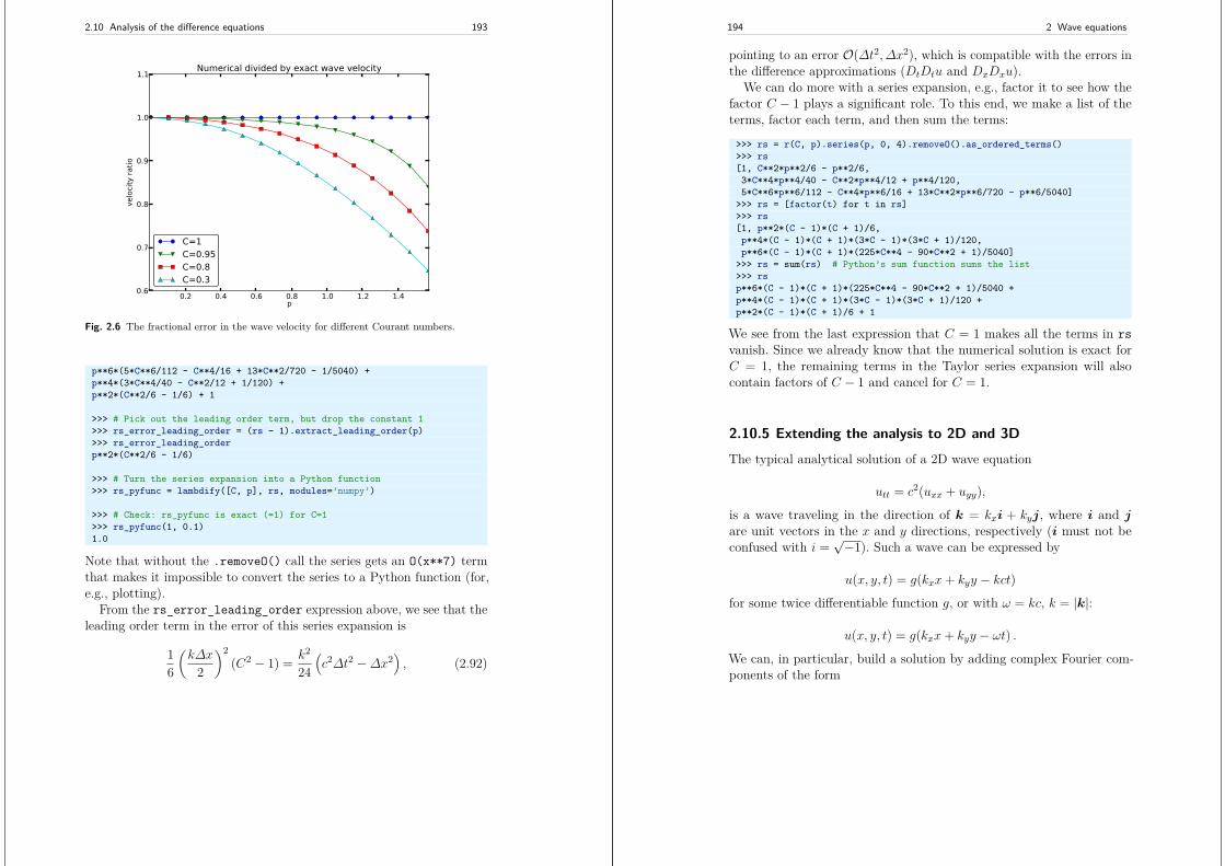
2.10 Analysis of the difference equations 193
0.2 0.4 0.6 0.8 1.0 1.2 1.4p
0.6
0.7
0.8
0.9
1.0
1.1
velo
city
ratio
Numerical divided by exact wave velocity
C=1C=0.95C=0.8C=0.3
Fig. 2.6 The fractional error in the wave velocity for different Courant numbers.
p**6*(5*C**6/112 - C**4/16 + 13*C**2/720 - 1/5040) +p**4*(3*C**4/40 - C**2/12 + 1/120) +p**2*(C**2/6 - 1/6) + 1
>>> # Pick out the leading order term, but drop the constant 1>>> rs_error_leading_order = (rs - 1).extract_leading_order(p)>>> rs_error_leading_orderp**2*(C**2/6 - 1/6)
>>> # Turn the series expansion into a Python function>>> rs_pyfunc = lambdify([C, p], rs, modules=’numpy’)
>>> # Check: rs_pyfunc is exact (=1) for C=1>>> rs_pyfunc(1, 0.1)1.0
Note that without the .removeO() call the series gets an O(x**7) termthat makes it impossible to convert the series to a Python function (for,e.g., plotting).
From the rs_error_leading_order expression above, we see that theleading order term in the error of this series expansion is
16
(k∆x
2
)2(C2 − 1) = k2
24(c2∆t2 −∆x2
), (2.92)
194 2 Wave equations
pointing to an error O(∆t2, ∆x2), which is compatible with the errors inthe difference approximations (DtDtu and DxDxu).
We can do more with a series expansion, e.g., factor it to see how thefactor C − 1 plays a significant role. To this end, we make a list of theterms, factor each term, and then sum the terms:
>>> rs = r(C, p).series(p, 0, 4).removeO().as_ordered_terms()>>> rs[1, C**2*p**2/6 - p**2/6,3*C**4*p**4/40 - C**2*p**4/12 + p**4/120,5*C**6*p**6/112 - C**4*p**6/16 + 13*C**2*p**6/720 - p**6/5040]
>>> rs = [factor(t) for t in rs]>>> rs[1, p**2*(C - 1)*(C + 1)/6,p**4*(C - 1)*(C + 1)*(3*C - 1)*(3*C + 1)/120,p**6*(C - 1)*(C + 1)*(225*C**4 - 90*C**2 + 1)/5040]
>>> rs = sum(rs) # Python’s sum function sums the list>>> rsp**6*(C - 1)*(C + 1)*(225*C**4 - 90*C**2 + 1)/5040 +p**4*(C - 1)*(C + 1)*(3*C - 1)*(3*C + 1)/120 +p**2*(C - 1)*(C + 1)/6 + 1
We see from the last expression that C = 1 makes all the terms in rsvanish. Since we already know that the numerical solution is exact forC = 1, the remaining terms in the Taylor series expansion will alsocontain factors of C − 1 and cancel for C = 1.
2.10.5 Extending the analysis to 2D and 3DThe typical analytical solution of a 2D wave equation
utt = c2(uxx + uyy),
is a wave traveling in the direction of k = kxi + kyj, where i and jare unit vectors in the x and y directions, respectively (i must not beconfused with i =
√−1). Such a wave can be expressed by
u(x, y, t) = g(kxx+ kyy − kct)for some twice differentiable function g, or with ω = kc, k = |k|:
u(x, y, t) = g(kxx+ kyy − ωt) .We can, in particular, build a solution by adding complex Fourier com-ponents of the form
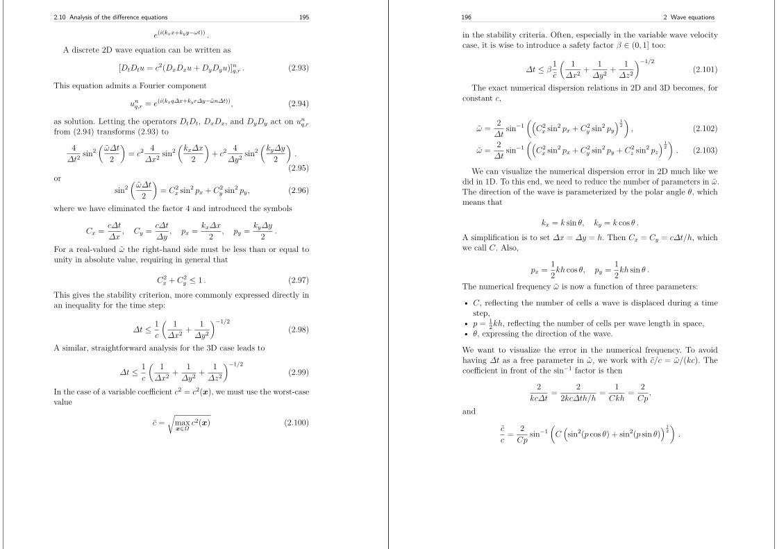
2.10 Analysis of the difference equations 195
e(i(kxx+kyy−ωt)) .
A discrete 2D wave equation can be written as
[DtDtu = c2(DxDxu+DyDyu)]nq,r . (2.93)
This equation admits a Fourier component
unq,r = e(i(kxq∆x+kyr∆y−ωn∆t)), (2.94)
as solution. Letting the operators DtDt, DxDx, and DyDy act on unq,rfrom (2.94) transforms (2.93) to
4∆t2
sin2(ω∆t
2
)= c2 4
∆x2 sin2(kx∆x
2
)+ c2 4
∆y2 sin2(ky∆y
2
).
(2.95)or
sin2(ω∆t
2
)= C2
x sin2 px + C2y sin2 py, (2.96)
where we have eliminated the factor 4 and introduced the symbols
Cx = c∆t
∆x, Cy = c∆t
∆y, px = kx∆x
2 , py = ky∆y
2 .
For a real-valued ω the right-hand side must be less than or equal tounity in absolute value, requiring in general that
C2x + C2
y ≤ 1 . (2.97)
This gives the stability criterion, more commonly expressed directly inan inequality for the time step:
∆t ≤ 1c
( 1∆x2 + 1
∆y2
)−1/2(2.98)
A similar, straightforward analysis for the 3D case leads to
∆t ≤ 1c
( 1∆x2 + 1
∆y2 + 1∆z2
)−1/2(2.99)
In the case of a variable coefficient c2 = c2(x), we must use the worst-casevalue
c =√
maxx∈Ω
c2(x) (2.100)
196 2 Wave equations
in the stability criteria. Often, especially in the variable wave velocitycase, it is wise to introduce a safety factor β ∈ (0, 1] too:
∆t ≤ β1c
( 1∆x2 + 1
∆y2 + 1∆z2
)−1/2(2.101)
The exact numerical dispersion relations in 2D and 3D becomes, forconstant c,
ω = 2∆t
sin−1((C2x sin2 px + C2
y sin2 py) 1
2), (2.102)
ω = 2∆t
sin−1((C2x sin2 px + C2
y sin2 py + C2z sin2 pz
) 12). (2.103)
We can visualize the numerical dispersion error in 2D much like wedid in 1D. To this end, we need to reduce the number of parameters in ω.The direction of the wave is parameterized by the polar angle θ, whichmeans that
kx = k sin θ, ky = k cos θ .
A simplification is to set ∆x = ∆y = h. Then Cx = Cy = c∆t/h, whichwe call C. Also,
px = 12kh cos θ, py = 1
2kh sin θ .
The numerical frequency ω is now a function of three parameters:
• C, reflecting the number of cells a wave is displaced during a timestep,
• p = 12kh, reflecting the number of cells per wave length in space,
• θ, expressing the direction of the wave.
We want to visualize the error in the numerical frequency. To avoidhaving ∆t as a free parameter in ω, we work with c/c = ω/(kc). Thecoefficient in front of the sin−1 factor is then
2kc∆t
= 22kc∆th/h = 1
Ckh= 2Cp
,
and
c
c= 2Cp
sin−1(C(sin2(p cos θ) + sin2(p sin θ)
) 12).
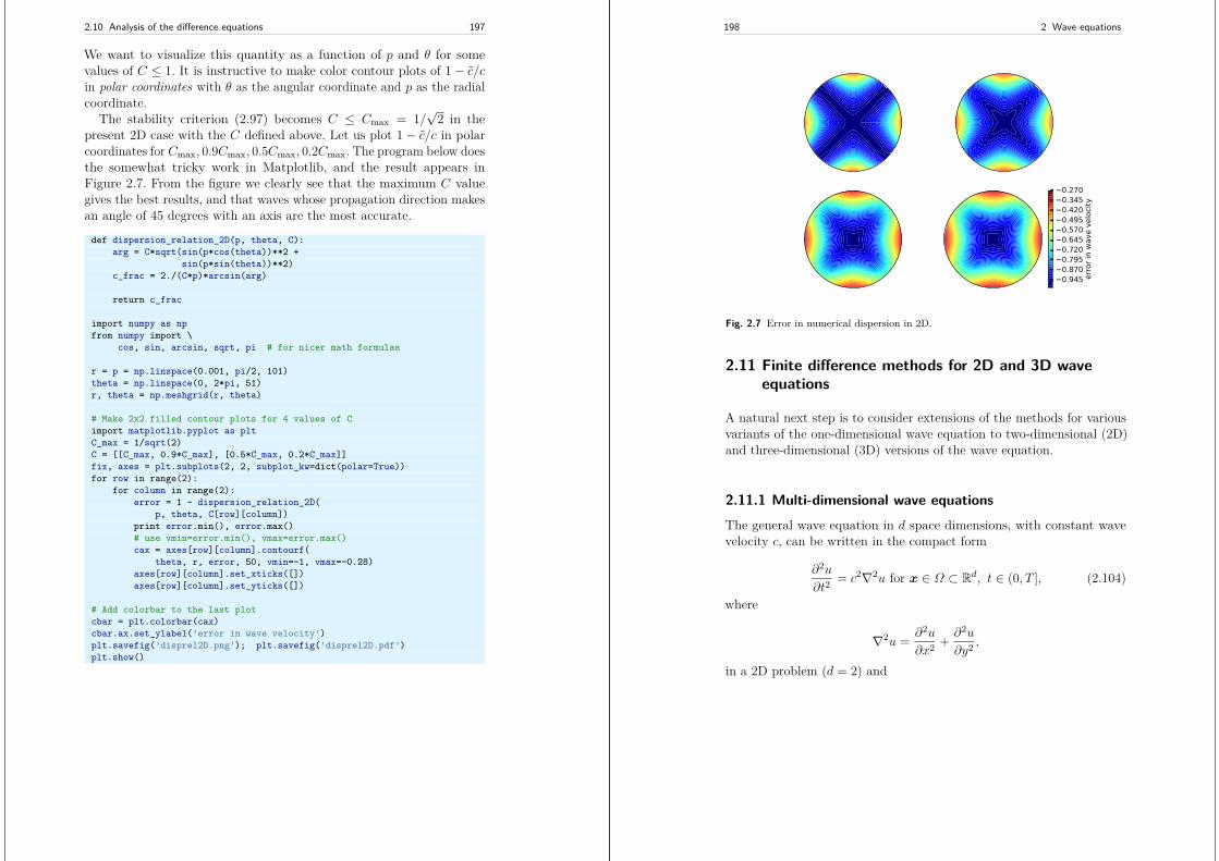
2.10 Analysis of the difference equations 197
We want to visualize this quantity as a function of p and θ for somevalues of C ≤ 1. It is instructive to make color contour plots of 1− c/cin polar coordinates with θ as the angular coordinate and p as the radialcoordinate.
The stability criterion (2.97) becomes C ≤ Cmax = 1/√
2 in thepresent 2D case with the C defined above. Let us plot 1− c/c in polarcoordinates for Cmax, 0.9Cmax, 0.5Cmax, 0.2Cmax. The program below doesthe somewhat tricky work in Matplotlib, and the result appears inFigure 2.7. From the figure we clearly see that the maximum C valuegives the best results, and that waves whose propagation direction makesan angle of 45 degrees with an axis are the most accurate.
def dispersion_relation_2D(p, theta, C):arg = C*sqrt(sin(p*cos(theta))**2 +
sin(p*sin(theta))**2)c_frac = 2./(C*p)*arcsin(arg)
return c_frac
import numpy as npfrom numpy import \
cos, sin, arcsin, sqrt, pi # for nicer math formulas
r = p = np.linspace(0.001, pi/2, 101)theta = np.linspace(0, 2*pi, 51)r, theta = np.meshgrid(r, theta)
# Make 2x2 filled contour plots for 4 values of Cimport matplotlib.pyplot as pltC_max = 1/sqrt(2)C = [[C_max, 0.9*C_max], [0.5*C_max, 0.2*C_max]]fix, axes = plt.subplots(2, 2, subplot_kw=dict(polar=True))for row in range(2):
for column in range(2):error = 1 - dispersion_relation_2D(
p, theta, C[row][column])print error.min(), error.max()# use vmin=error.min(), vmax=error.max()cax = axes[row][column].contourf(
theta, r, error, 50, vmin=-1, vmax=-0.28)axes[row][column].set_xticks([])axes[row][column].set_yticks([])
# Add colorbar to the last plotcbar = plt.colorbar(cax)cbar.ax.set_ylabel(’error in wave velocity’)plt.savefig(’disprel2D.png’); plt.savefig(’disprel2D.pdf’)plt.show()
198 2 Wave equations
0.9450.8700.7950.7200.6450.5700.4950.4200.3450.270
erro
r in
wav
e ve
loci
ty
Fig. 2.7 Error in numerical dispersion in 2D.
2.11 Finite difference methods for 2D and 3D waveequations
A natural next step is to consider extensions of the methods for variousvariants of the one-dimensional wave equation to two-dimensional (2D)and three-dimensional (3D) versions of the wave equation.
2.11.1 Multi-dimensional wave equationsThe general wave equation in d space dimensions, with constant wavevelocity c, can be written in the compact form
∂2u
∂t2= c2∇2u for x ∈ Ω ⊂ Rd, t ∈ (0, T ], (2.104)
where
∇2u = ∂2u
∂x2 + ∂2u
∂y2 ,
in a 2D problem (d = 2) and
2.11 Finite difference methods for 2D and 3D wave equations 199
∇2u = ∂2u
∂x2 + ∂2u
∂y2 + ∂2u
∂z2 ,
in three space dimensions (d = 3).Many applications involve variable coefficients, and the general wave
equation in d dimensions is in this case written as
%∂2u
∂t2= ∇ · (q∇u) + f for x ∈ Ω ⊂ Rd, t ∈ (0, T ], (2.105)
which in, e.g., 2D becomes
%(x, y)∂2u
∂t2= ∂
∂x
(q(x, y)∂u
∂x
)+ ∂
∂y
(q(x, y)∂u
∂y
)+ f(x, y, t) . (2.106)
To save some writing and space we may use the index notation, wheresubscript t, x, or y means differentiation with respect to that coordinate.For example,
∂2u
∂t2= utt,
∂
∂y
(q(x, y)∂u
∂y
)= (quy)y .
These comments extend straightforwardly to 3D, which means that the3D versions of the two wave PDEs, with and without variable coefficients,can be stated as
utt = c2(uxx + uyy + uzz) + f, (2.107)%utt = (qux)x + (quz)z + (quz)z + f . (2.108)
At each point of the boundary ∂Ω (of Ω) we need one boundarycondition involving the unknown u. The boundary conditions are of threeprincipal types:
1. u is prescribed (u = 0 or a known time variation of u at the boundarypoints, e.g., modeling an incoming wave),
2. ∂u/∂n = n · ∇u is prescribed (zero for reflecting boundaries),
200 2 Wave equations
3. an open boundary condition (also called radiation condition) is speci-fied to let waves travel undisturbed out of the domain, see Exercise 2.12for details.
All the listed wave equations with second-order derivatives in time needtwo initial conditions:
1. u = I,2. ut = V .
2.11.2 Mesh
We introduce a mesh in time and in space. The mesh in time consists oftime points
t0 = 0 < t1 < · · · < tNt ,
normally, for wave equation problems, with a constant spacing ∆t =tn+1 − tn, n ∈ I−t .
Finite difference methods are easy to implement on simple rectangle-or box-shaped spatial domains. More complicated shapes of the spatialdomain require substantially more advanced techniques and implementa-tional efforts (and a finite element method is usually a more convenientapproach). On a rectangle- or box-shaped domain, mesh points areintroduced separately in the various space directions:
x0 < x1 < · · · < xNx in the x direction,y0 < y1 < · · · < yNy in the y direction,z0 < z1 < · · · < zNz in the z direction .
We can write a general mesh point as (xi, yj , zk, tn), with i ∈ Ix, j ∈ Iy,k ∈ Iz, and n ∈ It.
It is a very common choice to use constant mesh spacings: ∆x =xi+1 − xi, i ∈ I−x , ∆y = yj+1 − yj , j ∈ I−y , and ∆z = zk+1 − zk, k ∈ I−z .With equal mesh spacings one often introduces h = ∆x = ∆y = ∆z.
The unknown u at mesh point (xi, yj , zk, tn) is denoted by uni,j,k. In2D problems we just skip the z coordinate (by assuming no variation inthat direction: ∂/∂z = 0) and write uni,j .
2.11 Finite difference methods for 2D and 3D wave equations 201
2.11.3 Discretization
Two- and three-dimensional wave equations are easily discretized by as-sembling building blocks for discretization of 1D wave equations, becausethe multi-dimensional versions just contain terms of the same type asthose in 1D.
Discretizing the PDEs. Equation (2.107) can be discretized as
[DtDtu = c2(DxDxu+DyDyu+DzDzu) + f ]ni,j,k . (2.109)
A 2D version might be instructive to write out in detail:
[DtDtu = c2(DxDxu+DyDyu) + f ]ni,j,k,
which becomes
un+1i,j − 2uni,j + un−1
i,j
∆t2= c2u
ni+1,j − 2uni,j + uni−1,j
∆x2 +c2uni,j+1 − 2uni,j + uni,j−1
∆y2 +fni,j ,
Assuming, as usual, that all values at time levels n and n− 1 are known,we can solve for the only unknown un+1
i,j . The result can be compactlywritten as
un+1i,j = 2uni,j + un−1
i,j + c2∆t2[DxDxu+DyDyu]ni,j . (2.110)
As in the 1D case, we need to develop a special formula for u1i,j
where we combine the general scheme for un+1i,j , when n = 0, with the
discretization of the initial condition:
[D2tu = V ]0i,j ⇒ u−1i,j = u1
i,j − 2∆tVi,j .
The result becomes, in compact form,
u1i,j = u0
i,j − 2∆Vi,j + 12c
2∆t2[DxDxu+DyDyu]0i,j . (2.111)
The PDE (2.108) with variable coefficients is discretized term by termusing the corresponding elements from the 1D case:
[%DtDtu = (DxqxDxu+Dyq
yDyu+DzqzDzu) + f ]ni,j,k . (2.112)
202 2 Wave equations
When written out and solved for the unknown un+1i,j,k , one gets the scheme
un+1i,j,k = −un−1
i,j,k + 2uni,j,k+1
%i,j,k
1∆x2 (1
2(qi,j,k + qi+1,j,k)(uni+1,j,k − uni,j,k)−
12(qi−1,j,k + qi,j,k)(uni,j,k − uni−1,j,k))+
1%i,j,k
1∆x2 (1
2(qi,j,k + qi,j+1,k)(uni,j+1,k − uni,j,k)−
12(qi,j−1,k + qi,j,k)(uni,j,k − uni,j−1,k))+
1%i,j,k
1∆x2 (1
2(qi,j,k + qi,j,k+1)(uni,j,k+1 − uni,j,k)−
12(qi,j,k−1 + qi,j,k)(uni,j,k − uni,j,k−1))+
∆t2fni,j,k .
Also here we need to develop a special formula for u1i,j,k by combining
the scheme for n = 0 with the discrete initial condition, which is just amatter of inserting u−1
i,j,k = u1i,j,k − 2∆tVi,j,k in the scheme and solving
for u1i,j,k.
Handling boundary conditions where u is known. The schemes listedabove are valid for the internal points in the mesh. After updatingthese, we need to visit all the mesh points at the boundaries and set theprescribed u value.
Discretizing the Neumann condition. The condition ∂u/∂n = 0 wasimplemented in 1D by discretizing it with a D2xu centered difference,followed by eliminating the fictitious u point outside the mesh by using thegeneral scheme at the boundary point. Alternatively, one can introduceghost cells and update a ghost value for use in the Neumann condition.Exactly the same ideas are reused in multiple dimensions.
Consider the condition ∂u/∂n = 0 at a boundary y = 0 of a rectangulardomain [0, Lx]×[0, Ly] in 2D. The normal direction is then in−y direction,so
∂u
∂n= −∂u
∂y,
and we set
2.12 Implementation 203
[−D2yu = 0]ni,0 ⇒ uni,1 − uni,−12∆y = 0 .
From this it follows that uni,−1 = uni,1. The discretized PDE at theboundary point (i, 0) reads
un+1i,0 − 2uni,0 + un−1
i,0∆t2
= c2uni+1,0 − 2uni,0 + uni−1,0
∆x2 +c2uni,1 − 2uni,0 + uni,−1
∆y2 +fni,j ,
We can then just insert uni,1 for uni,−1 in this equation and solve for theboundary value un+1
i,0 , just as was done in 1D.From these calculations, we see a pattern: the general scheme applies
at the boundary j = 0 too if we just replace j−1 by j+1. Such a patternis particularly useful for implementations. The details follow from theexplained 1D case in Section 2.6.3.
The alternative approach to eliminating fictitious values outside themesh is to have uni,−1 available as a ghost value. The mesh is extendedwith one extra line (2D) or plane (3D) of ghost cells at a Neumannboundary. In the present example it means that we need a line with ghostcells below the y axis. The ghost values must be updated according toun+1i,−1 = un+1
i,1 .
2.12 Implementation
We shall now describe in detail various Python implementations forsolving a standard 2D, linear wave equation with constant wave velocityand u = 0 on the boundary. The wave equation is to be solved in the space-time domainΩ×(0, T ], whereΩ = (0, Lx)×(0, Ly) is a rectangular spatialdomain. More precisely, the complete initial-boundary value problem isdefined by
utt = c2(uxx + uyy) + f(x, y, t), (x, y) ∈ Ω, t ∈ (0, T ], (2.113)u(x, y, 0) = I(x, y), (x, y) ∈ Ω, (2.114)ut(x, y, 0) = V (x, y), (x, y) ∈ Ω, (2.115)u = 0, (x, y) ∈ ∂Ω, t ∈ (0, T ], (2.116)
where ∂Ω is the boundary of Ω, in this case the four sides of the rectangleΩ = [0, Lx]× [0, Ly]: x = 0, x = Lx, y = 0, and y = Ly.
204 2 Wave equations
The PDE is discretized as
[DtDtu = c2(DxDxu+DyDyu) + f ]ni,j ,
which leads to an explicit updating formula to be implemented in aprogram:
un+1i,j = −un−1
i,j + 2uni,j+C2x(uni+1,j − 2uni,j + uni−1,j) + C2
y (uni,j+1 − 2uni,j + uni,j−1) +∆t2fni,j ,
(2.117)
for all interior mesh points i ∈ Iix and j ∈ Iiy, for n ∈ I+t . The constants
Cx and Cy are defined as
Cx = c∆t
∆x, Cx = c
∆t
∆y.
At the boundary, we simply set un+1i,j = 0 for i = 0, j = 0, . . . , Ny;
i = Nx, j = 0, . . . , Ny; j = 0, i = 0, . . . , Nx; and j = Ny, i = 0, . . . , Nx.For the first step, n = 0, (2.117) is combined with the discretization ofthe initial condition ut = V , [D2tu = V ]0i,j to obtain a special formulafor u1
i,j at the interior mesh points:
u1i,j = u0
i,j +∆tVi,j+12C
2x(u0
i+1,j − 2u0i,j + u0
i−1,j) + 12C
2y (u0
i,j+1 − 2u0i,j + u0
i,j−1)+12∆t
2fni,j , (2.118)
The algorithm is very similar to the one in 1D:
1. Set initial condition u0i,j = I(xi, yj)
2. Compute u1i,j from (2.117)
3. Set u1i,j = 0 for the boundaries i = 0, Nx, j = 0, Ny
4. For n = 1, 2, . . . , Nt:a. Find un+1
i,j from (2.117) for all internal mesh points, i ∈ Iix, j ∈ Iiyb. Set un+1
i,j = 0 for the boundaries i = 0, Nx, j = 0, Ny
2.12 Implementation 205
2.12.1 Scalar computations
The solver function for a 2D case with constant wave velocity and bound-ary condition u = 0 is analogous to the 1D case with similar parametervalues (see wave1D_u0.py), apart from a few necessary extensions. Thecode is found in the program wave2D_u0.py.
Domain and mesh. The spatial domain is now [0, Lx]× [0, Ly], specifiedby the arguments Lx and Ly. Similarly, the number of mesh points inthe x and y directions, Nx and Ny, become the arguments Nx and Ny.In multi-dimensional problems it makes less sense to specify a Courantnumber since the wave velocity is a vector and mesh spacings may differin the various spatial directions. We therefore give ∆t explicitly. Thesignature of the solver function is then
def solver(I, V, f, c, Lx, Ly, Nx, Ny, dt, T,user_action=None, version=’scalar’):
Key parameters used in the calculations are created as
x = linspace(0, Lx, Nx+1) # mesh points in x diry = linspace(0, Ly, Ny+1) # mesh points in y dirdx = x[1] - x[0]dy = y[1] - y[0]Nt = int(round(T/float(dt)))t = linspace(0, N*dt, N+1) # mesh points in timeCx2 = (c*dt/dx)**2; Cy2 = (c*dt/dy)**2 # help variablesdt2 = dt**2
Solution arrays. We store un+1i,j , uni,j , and un−1
i,j in three two-dimensionalarrays,
u = zeros((Nx+1,Ny+1)) # solution arrayu_n = [zeros((Nx+1,Ny+1)), zeros((Nx+1,Ny+1))] # t-dt, t-2*dt
where un+1i,j corresponds to u[i,j], uni,j to u_n[i,j], and un−1
i,j tou_nm1[i,j].
Index sets. It is also convenient to introduce the index sets (cf. Sec-tion 2.6.4)
Ix = range(0, u.shape[0])Iy = range(0, u.shape[1])It = range(0, t.shape[0])
Computing the solution. Inserting the initial condition I in u_n andmaking a callback to the user in terms of the user_action function is astraightforward generalization of the 1D code from Section 2.1.6:
206 2 Wave equations
for i in Ix:for j in Iy:
u_n[i,j] = I(x[i], y[j])
if user_action is not None:user_action(u_n, x, xv, y, yv, t, 0)
The user_action function has additional arguments compared to the 1Dcase. The arguments xv and yv will be commented upon in Section 2.12.2.
The key finite difference formula (2.110) for updating the solution ata time level is implemented in a separate function as
def advance_scalar(u, u_n, u_nm1, f, x, y, t, n, Cx2, Cy2, dt2,V=None, step1=False):
Ix = range(0, u.shape[0]); Iy = range(0, u.shape[1])if step1:
dt = sqrt(dt2) # saveCx2 = 0.5*Cx2; Cy2 = 0.5*Cy2; dt2 = 0.5*dt2 # redefineD1 = 1; D2 = 0
else:D1 = 2; D2 = 1
for i in Ix[1:-1]:for j in Iy[1:-1]:
u_xx = u_n[i-1,j] - 2*u_n[i,j] + u_n[i+1,j]u_yy = u_n[i,j-1] - 2*u_n[i,j] + u_n[i,j+1]u[i,j] = D1*u_n[i,j] - D2*u_nm1[i,j] + \
Cx2*u_xx + Cy2*u_yy + dt2*f(x[i], y[j], t[n])if step1:
u[i,j] += dt*V(x[i], y[j])# Boundary condition u=0j = Iy[0]for i in Ix: u[i,j] = 0j = Iy[-1]for i in Ix: u[i,j] = 0i = Ix[0]for j in Iy: u[i,j] = 0i = Ix[-1]for j in Iy: u[i,j] = 0return u
The step1 variable has been introduced to allow the formula to be reusedfor the first step, computing u1
i,j :
u = advance_scalar(u, u_n, f, x, y, t,n, Cx2, Cy2, dt, V, step1=True)
Below, we will make many alternative implementations of theadvance_scalar function to speed up the code since most of theCPU time in simulations is spent in this function.
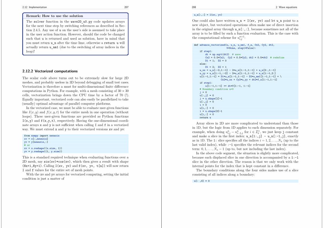
2.12 Implementation 207
Remark: How to use the solutionThe solver function in the wave2D_u0.py code updates arraysfor the next time step by switching references as described in Sec-tion 2.4.5. Any use of u on the user’s side is assumed to take placein the user action function. However, should the code be changedsuch that u is returned and used as solution, have in mind thatyou must return u_n after the time lime, otherwise a return u willactually return u_nm1 (due to the switching of array indices in theloop)!
2.12.2 Vectorized computations
The scalar code above turns out to be extremely slow for large 2Dmeshes, and probably useless in 3D beyond debugging of small test cases.Vectorization is therefore a must for multi-dimensional finite differencecomputations in Python. For example, with a mesh consisting of 30× 30cells, vectorization brings down the CPU time by a factor of 70 (!).Equally important, vectorized code can also easily be parallelized to take(usually) optimal advantage of parallel computer platforms.
In the vectorized case, we must be able to evaluate user-given functionslike I(x, y) and f(x, y, t) for the entire mesh in one operation (withoutloops). These user-given functions are provided as Python functionsI(x,y) and f(x,y,t), respectively. Having the one-dimensional coordi-nate arrays x and y is not sufficient when calling I and f in a vectorizedway. We must extend x and y to their vectorized versions xv and yv:
from numpy import newaxisxv = x[:,newaxis]yv = y[newaxis,:]# orxv = x.reshape((x.size, 1))yv = y.reshape((1, y.size))
This is a standard required technique when evaluating functions over a2D mesh, say sin(xv)*cos(xv), which then gives a result with shape(Nx+1,Ny+1). Calling I(xv, yv) and f(xv, yv, t[n]) will now returnI and f values for the entire set of mesh points.
With the xv and yv arrays for vectorized computing, setting the initialcondition is just a matter of
208 2 Wave equations
u_n[:,:] = I(xv, yv)
One could also have written u_n = I(xv, yv) and let u_n point to anew object, but vectorized operations often make use of direct insertionin the original array through u_n[:,:], because sometimes not all of thearray is to be filled by such a function evaluation. This is the case withthe computational scheme for un+1
i,j :
def advance_vectorized(u, u_n, u_nm1, f_a, Cx2, Cy2, dt2,V=None, step1=False):
if step1:dt = np.sqrt(dt2) # saveCx2 = 0.5*Cx2; Cy2 = 0.5*Cy2; dt2 = 0.5*dt2 # redefineD1 = 1; D2 = 0
else:D1 = 2; D2 = 1
u_xx = u_n[:-2,1:-1] - 2*u_n[1:-1,1:-1] + u_n[2:,1:-1]u_yy = u_n[1:-1,:-2] - 2*u_n[1:-1,1:-1] + u_n[1:-1,2:]u[1:-1,1:-1] = D1*u_n[1:-1,1:-1] - D2*u_nm1[1:-1,1:-1] + \
Cx2*u_xx + Cy2*u_yy + dt2*f_a[1:-1,1:-1]if step1:
u[1:-1,1:-1] += dt*V[1:-1, 1:-1]# Boundary condition u=0j = 0u[:,j] = 0j = u.shape[1]-1u[:,j] = 0i = 0u[i,:] = 0i = u.shape[0]-1u[i,:] = 0return u
Array slices in 2D are more complicated to understand than thosein 1D, but the logic from 1D applies to each dimension separately. Forexample, when doing uni,j − uni−1,j for i ∈ I+
x , we just keep j constantand make a slice in the first index: u_n[1:,j] - u_n[:-1,j], exactlyas in 1D. The 1: slice specifies all the indices i = 1, 2, . . . , Nx (up to thelast valid index), while :-1 specifies the relevant indices for the secondterm: 0, 1, . . . , Nx − 1 (up to, but not including the last index).
In the above code segment, the situation is slightly more complicated,because each displaced slice in one direction is accompanied by a 1:-1slice in the other direction. The reason is that we only work with theinternal points for the index that is kept constant in a difference.
The boundary conditions along the four sides makes use of a sliceconsisting of all indices along a boundary:
u[: ,0] = 0
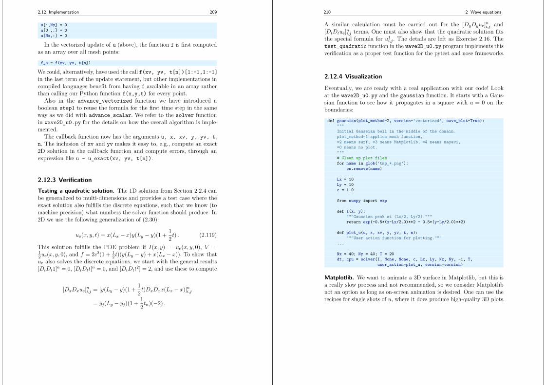
2.12 Implementation 209
u[:,Ny] = 0u[0 ,:] = 0u[Nx,:] = 0
In the vectorized update of u (above), the function f is first computedas an array over all mesh points:
f_a = f(xv, yv, t[n])
We could, alternatively, have used the call f(xv, yv, t[n])[1:-1,1:-1]in the last term of the update statement, but other implementations incompiled languages benefit from having f available in an array ratherthan calling our Python function f(x,y,t) for every point.
Also in the advance_vectorized function we have introduced aboolean step1 to reuse the formula for the first time step in the sameway as we did with advance_scalar. We refer to the solver functionin wave2D_u0.py for the details on how the overall algorithm is imple-mented.
The callback function now has the arguments u, x, xv, y, yv, t,n. The inclusion of xv and yv makes it easy to, e.g., compute an exact2D solution in the callback function and compute errors, through anexpression like u - u_exact(xv, yv, t[n]).
2.12.3 VerificationTesting a quadratic solution. The 1D solution from Section 2.2.4 canbe generalized to multi-dimensions and provides a test case where theexact solution also fulfills the discrete equations, such that we know (tomachine precision) what numbers the solver function should produce. In2D we use the following generalization of (2.30):
ue(x, y, t) = x(Lx − x)y(Ly − y)(1 + 12 t) . (2.119)
This solution fulfills the PDE problem if I(x, y) = ue(x, y, 0), V =12ue(x, y, 0), and f = 2c2(1 + 1
2 t)(y(Ly − y) + x(Lx − x)). To show thatue also solves the discrete equations, we start with the general results[DtDt1]n = 0, [DtDtt]n = 0, and [DtDtt
2] = 2, and use these to compute
[DxDxue]ni,j = [y(Ly − y)(1 + 12 t)DxDxx(Lx − x)]ni,j
= yj(Ly − yj)(1 + 12 tn)(−2) .
210 2 Wave equations
A similar calculation must be carried out for the [DyDyue]ni,j and[DtDtue]ni,j terms. One must also show that the quadratic solution fitsthe special formula for u1
i,j . The details are left as Exercise 2.16. Thetest_quadratic function in the wave2D_u0.py program implements thisverification as a proper test function for the pytest and nose frameworks.
2.12.4 Visualization
Eventually, we are ready with a real application with our code! Lookat the wave2D_u0.py and the gaussian function. It starts with a Gaus-sian function to see how it propagates in a square with u = 0 on theboundaries:
def gaussian(plot_method=2, version=’vectorized’, save_plot=True):"""Initial Gaussian bell in the middle of the domain.plot_method=1 applies mesh function,=2 means surf, =3 means Matplotlib, =4 means mayavi,=0 means no plot."""# Clean up plot filesfor name in glob(’tmp_*.png’):
os.remove(name)
Lx = 10Ly = 10c = 1.0
from numpy import exp
def I(x, y):"""Gaussian peak at (Lx/2, Ly/2)."""return exp(-0.5*(x-Lx/2.0)**2 - 0.5*(y-Ly/2.0)**2)
def plot_u(u, x, xv, y, yv, t, n):"""User action function for plotting."""
...
Nx = 40; Ny = 40; T = 20dt, cpu = solver(I, None, None, c, Lx, Ly, Nx, Ny, -1, T,
user_action=plot_u, version=version)
Matplotlib. We want to animate a 3D surface in Matplotlib, but this isa really slow process and not recommended, so we consider Matplotlibnot an option as long as on-screen animation is desired. One can use therecipes for single shots of u, where it does produce high-quality 3D plots.
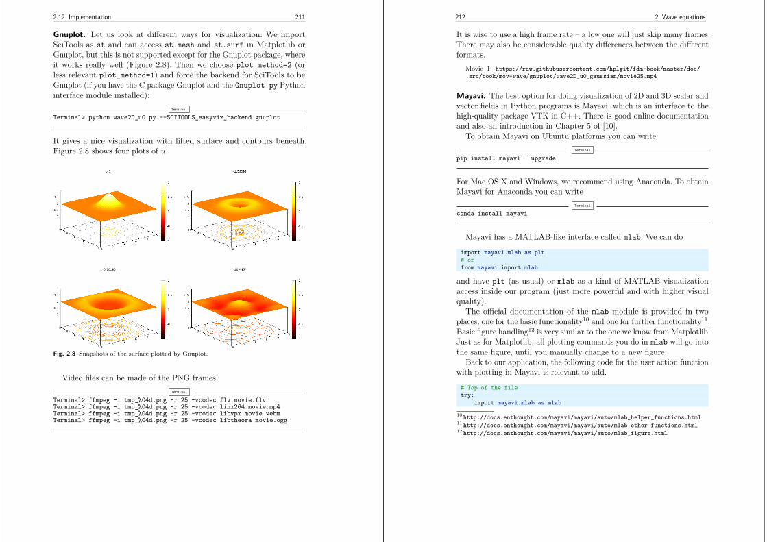
2.12 Implementation 211
Gnuplot. Let us look at different ways for visualization. We importSciTools as st and can access st.mesh and st.surf in Matplotlib orGnuplot, but this is not supported except for the Gnuplot package, whereit works really well (Figure 2.8). Then we choose plot_method=2 (orless relevant plot_method=1) and force the backend for SciTools to beGnuplot (if you have the C package Gnuplot and the Gnuplot.py Pythoninterface module installed):
Terminal
Terminal> python wave2D_u0.py --SCITOOLS_easyviz_backend gnuplot
It gives a nice visualization with lifted surface and contours beneath.Figure 2.8 shows four plots of u.
Fig. 2.8 Snapshots of the surface plotted by Gnuplot.
Video files can be made of the PNG frames:Terminal
Terminal> ffmpeg -i tmp_%04d.png -r 25 -vcodec flv movie.flvTerminal> ffmpeg -i tmp_%04d.png -r 25 -vcodec linx264 movie.mp4Terminal> ffmpeg -i tmp_%04d.png -r 25 -vcodec libvpx movie.webmTerminal> ffmpeg -i tmp_%04d.png -r 25 -vcodec libtheora movie.ogg
212 2 Wave equations
It is wise to use a high frame rate – a low one will just skip many frames.There may also be considerable quality differences between the differentformats.
Movie 1: https://raw.githubusercontent.com/hplgit/fdm-book/master/doc/.src/book/mov-wave/gnuplot/wave2D_u0_gaussian/movie25.mp4
Mayavi. The best option for doing visualization of 2D and 3D scalar andvector fields in Python programs is Mayavi, which is an interface to thehigh-quality package VTK in C++. There is good online documentationand also an introduction in Chapter 5 of [10].
To obtain Mayavi on Ubuntu platforms you can writeTerminal
pip install mayavi --upgrade
For Mac OS X and Windows, we recommend using Anaconda. To obtainMayavi for Anaconda you can write
Terminal
conda install mayavi
Mayavi has a MATLAB-like interface called mlab. We can do
import mayavi.mlab as plt# orfrom mayavi import mlab
and have plt (as usual) or mlab as a kind of MATLAB visualizationaccess inside our program (just more powerful and with higher visualquality).
The official documentation of the mlab module is provided in twoplaces, one for the basic functionality10 and one for further functionality11.Basic figure handling12 is very similar to the one we know from Matplotlib.Just as for Matplotlib, all plotting commands you do in mlab will go intothe same figure, until you manually change to a new figure.
Back to our application, the following code for the user action functionwith plotting in Mayavi is relevant to add.
# Top of the filetry:
import mayavi.mlab as mlab
10 http://docs.enthought.com/mayavi/mayavi/auto/mlab_helper_functions.html11 http://docs.enthought.com/mayavi/mayavi/auto/mlab_other_functions.html12 http://docs.enthought.com/mayavi/mayavi/auto/mlab_figure.html
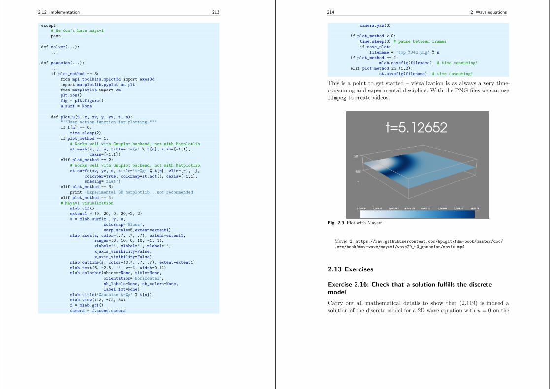
2.12 Implementation 213
except:# We don’t have mayavipass
def solver(...):...
def gaussian(...):...if plot_method == 3:
from mpl_toolkits.mplot3d import axes3dimport matplotlib.pyplot as pltfrom matplotlib import cmplt.ion()fig = plt.figure()u_surf = None
def plot_u(u, x, xv, y, yv, t, n):"""User action function for plotting."""if t[n] == 0:
time.sleep(2)if plot_method == 1:
# Works well with Gnuplot backend, not with Matplotlibst.mesh(x, y, u, title=’t=%g’ % t[n], zlim=[-1,1],
caxis=[-1,1])elif plot_method == 2:
# Works well with Gnuplot backend, not with Matplotlibst.surfc(xv, yv, u, title=’t=%g’ % t[n], zlim=[-1, 1],
colorbar=True, colormap=st.hot(), caxis=[-1,1],shading=’flat’)
elif plot_method == 3:print ’Experimental 3D matplotlib...not recommended’
elif plot_method == 4:# Mayavi visualization
mlab.clf()extent1 = (0, 20, 0, 20,-2, 2)s = mlab.surf(x , y, u,
colormap=’Blues’,warp_scale=5,extent=extent1)
mlab.axes(s, color=(.7, .7, .7), extent=extent1,ranges=(0, 10, 0, 10, -1, 1),xlabel=’’, ylabel=’’, zlabel=’’,x_axis_visibility=False,z_axis_visibility=False)
mlab.outline(s, color=(0.7, .7, .7), extent=extent1)mlab.text(6, -2.5, ’’, z=-4, width=0.14)mlab.colorbar(object=None, title=None,
orientation=’horizontal’,nb_labels=None, nb_colors=None,label_fmt=None)
mlab.title(’Gaussian t=%g’ % t[n])mlab.view(142, -72, 50)f = mlab.gcf()camera = f.scene.camera
214 2 Wave equations
camera.yaw(0)
if plot_method > 0:time.sleep(0) # pause between framesif save_plot:
filename = ’tmp_%04d.png’ % nif plot_method == 4:
mlab.savefig(filename) # time consuming!elif plot_method in (1,2):
st.savefig(filename) # time consuming!
This is a point to get started – visualization is as always a very time-consuming and experimental discipline. With the PNG files we can useffmpeg to create videos.
Fig. 2.9 Plot with Mayavi.
Movie 2: https://raw.githubusercontent.com/hplgit/fdm-book/master/doc/.src/book/mov-wave/mayavi/wave2D_u0_gaussian/movie.mp4
2.13 Exercises
Exercise 2.16: Check that a solution fulfills the discretemodelCarry out all mathematical details to show that (2.119) is indeed asolution of the discrete model for a 2D wave equation with u = 0 on the
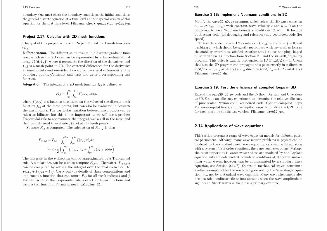
2.13 Exercises 215
boundary. One must check the boundary conditions, the initial conditions,the general discrete equation at a time level and the special version of thisequation for the first time level. Filename: check_quadratic_solution.
Project 2.17: Calculus with 2D mesh functionsThe goal of this project is to redo Project 2.6 with 2D mesh functions(fi,j).Differentiation. The differentiation results in a discrete gradient func-tion, which in the 2D case can be represented by a three-dimensionalarray df[d,i,j] where d represents the direction of the derivative, andi,j is a mesh point in 2D. Use centered differences for the derivativeat inner points and one-sided forward or backward differences at theboundary points. Construct unit tests and write a corresponding testfunction.Integration. The integral of a 2D mesh function fi,j is defined as
Fi,j =∫ yj
y0
∫ xi
x0
f(x, y)dxdy,
where f(x, y) is a function that takes on the values of the discrete meshfunction fi,j at the mesh points, but can also be evaluated in betweenthe mesh points. The particular variation between mesh points can betaken as bilinear, but this is not important as we will use a productTrapezoidal rule to approximate the integral over a cell in the mesh andthen we only need to evaluate f(x, y) at the mesh points.
Suppose Fi,j is computed. The calculation of Fi+1,j is then
Fi+1,j = Fi,j +∫ xi+1
xi
∫ yj
y0
f(x, y)dydx
≈ ∆x12
(∫ yj
y0
f(xi, y)dy +∫ yj
y0
f(xi+1, y)dy)
The integrals in the y direction can be approximated by a Trapezoidalrule. A similar idea can be used to compute Fi,j+1. Thereafter, Fi+1,j+1can be computed by adding the integral over the final corner cell toFi+1,j + Fi,j+1 − Fi,j . Carry out the details of these computations andimplement a function that can return Fi,j for all mesh indices i and j.Use the fact that the Trapezoidal rule is exact for linear functions andwrite a test function. Filename: mesh_calculus_2D.
216 2 Wave equations
Exercise 2.18: Implement Neumann conditions in 2D
Modify the wave2D_u0.py program, which solves the 2D wave equationutt = c2(uxx + uyy) with constant wave velocity c and u = 0 on theboundary, to have Neumann boundary conditions: ∂u/∂n = 0. Includeboth scalar code (for debugging and reference) and vectorized code (forspeed).
To test the code, use u = 1.2 as solution (I(x, y) = 1.2, V = f = 0, andc arbitrary), which should be exactly reproduced with any mesh as long asthe stability criterion is satisfied. Another test is to use the plug-shapedpulse in the pulse function from Section 2.8 and the wave1D_dn_vc.pyprogram. This pulse is exactly propagated in 1D if c∆t/∆x = 1. Checkthat also the 2D program can propagate this pulse exactly in x direction(c∆t/∆x = 1, ∆y arbitrary) and y direction (c∆t/∆y = 1, ∆x arbitrary).Filename: wave2D_dn.
Exercise 2.19: Test the efficiency of compiled loops in 3D
Extend the wave2D_u0.py code and the Cython, Fortran, and C versionsto 3D. Set up an efficiency experiment to determine the relative efficiencyof pure scalar Python code, vectorized code, Cython-compiled loops,Fortran-compiled loops, and C-compiled loops. Normalize the CPU timefor each mesh by the fastest version. Filename: wave3D_u0.
2.14 Applications of wave equations
This section presents a range of wave equation models for different physi-cal phenomena. Although many wave motion problems in physics can bemodeled by the standard linear wave equation, or a similar formulationwith a system of first-order equations, there are some exceptions. Perhapsthe most important is water waves: these are modeled by the Laplaceequation with time-dependent boundary conditions at the water surface(long water waves, however, can be approximated by a standard waveequation, see Section 2.14.7). Quantum mechanical waves constituteanother example where the waves are governed by the Schrödinger equa-tion, i.e., not by a standard wave equation. Many wave phenomena alsoneed to take nonlinear effects into account when the wave amplitude issignificant. Shock waves in the air is a primary example.
2.14 Applications of wave equations 217
The derivations in the following are very brief. Those with a firmbackground in continuum mechanics will probably have enough knowledgeto fill in the details, while other readers will hopefully get some impressionof the physics and approximations involved when establishing waveequation models.
2.14.1 Waves on a string
ui
ui−1
ui+1
xi xi+1xi−1
TT
Fig. 2.10 Discrete string model with point masses connected by elastic strings.
Figure 2.10 shows a model we may use to derive the equation forwaves on a string. The string is modeled as a set of discrete point
218 2 Wave equations
masses (at mesh points) with elastic strings in between. The string has alarge constant tension T . We let the mass at mesh point xi be mi. Thedisplacement of this mass point in the y direction is denoted by ui(t).
The motion of mass mi is governed by Newton’s second law of motion.The position of the mass at time t is xii+ ui(t)j, where i and j are unitvectors in the x and y direction, respectively. The acceleration is thenu′′i (t)j. Two forces are acting on the mass as indicated in Figure 2.10.The force T− acting toward the point xi−1 can be decomposed as
T− = −T sinφi− T cosφj,
where φ is the angle between the force and the line x = xi. Let ∆ui = ui−ui−1 and let ∆si =
√∆u2
i + (xi − xi−1)2 be the distance from mass mi−1to mass mi. It is seen that cosφ = ∆ui/∆si and sinφ = (xi − xi−1)/∆sor ∆x/∆si if we introduce a constant mesh spacing ∆x = xi− xi−1. Theforce can then be written
T− = −T ∆x∆si
i− T ∆ui∆si
j .
The force T+ acting toward xi+1 can be calculated in a similar way:
T+ = T∆x
∆si+1i+ T
∆ui+1∆si+1
j .
Newton’s second law becomes
miu′′i (t)j = T+ + T−,
which gives the component equations
T∆x
∆si= T
∆x
∆si+1, (2.120)
miu′′i (t) = T
∆ui+1∆si+1
− T ∆ui∆si
. (2.121)
A basic reasonable assumption for a string is small displacements uiand small displacement gradients ∆ui/∆x. For small g = ∆ui/∆x wehave that
∆si =√∆u2
i +∆x2 = ∆x√
1 + g2 +∆x(1 + 12g
2 +O(g4) ≈ ∆x .
2.14 Applications of wave equations 219
Equation (2.120) is then simply the identity T = T , while (2.121) can bewritten as
miu′′i (t) = T
∆ui+1∆x
− T ∆ui∆x
,
which upon division by ∆x and introducing the density %i = mi/∆xbecomes
%iu′′i (t) = T
1∆x2 (ui+1 − 2ui + ui−1) . (2.122)
We can now choose to approximate u′′i by a finite difference in time andget the discretized wave equation,
%i1∆t2
(un+1i − 2uni − un−1
i
)= T
1∆x2 (ui+1 − 2ui + ui−1) . (2.123)
On the other hand, we may go to the continuum limit ∆x → 0 andreplace ui(t) by u(x, t), %i by %(x), and recognize that the right-handside of (2.122) approaches ∂2u/∂x2 as ∆x → 0. We end up with thecontinuous model for waves on a string:
%∂2u
∂t2= T
∂2u
∂x2 . (2.124)
Note that the density % may change along the string, while the tension Tis a constant. With variable wave velocity c(x) =
√T/%(x) we can write
the wave equation in the more standard form
∂2u
∂t2= c2(x)∂
2u
∂x2 . (2.125)
Because of the way % enters the equations, the variable wave velocitydoes not appear inside the derivatives as in many other versions of thewave equation. However, most strings of interest have constant %.
The end points of a string are fixed so that the displacement u is zero.The boundary conditions are therefore u = 0.
Damping. Air resistance and non-elastic effects in the string will con-tribute to reduce the amplitudes of the waves so that the motion diesout after some time. This damping effect can be modeled by a term buton the left-hand side of the equation
%∂2u
∂t2+ b
∂u
∂t= T
∂2u
∂x2 . (2.126)
220 2 Wave equations
The parameter b ≥ 0 is small for most wave phenomena, but the dampingeffect may become significant in long time simulations.External forcing. It is easy to include an external force acting on thestring. Say we have a vertical force fij acting on mass mi, modeling theeffect of gravity on a string. This force affects the vertical component ofNewton’s law and gives rise to an extra term f(x, t) on the right-handside of (2.124). In the model (2.125) we would add a term f(x, t) =f(x, t)/%(x).Modeling the tension via springs. We assumed, in the derivation above,that the tension in the string, T , was constant. It is easy to check thisassumption by modeling the string segments between the masses asstandard springs, where the force (tension T ) is proportional to theelongation of the spring segment. Let k be the spring constant, and setTi = k∆` for the tension in the spring segment between xi−1 and xi,where ∆` is the elongation of this segment from the tension-free state.A basic feature of a string is that it has high tension in the equilibriumposition u = 0. Let the string segment have an elongation ∆`0 in theequilibrium position. After deformation of the string, the elongation is∆` = ∆`0 +∆si: Ti = k(∆`0 +∆si) ≈ k(∆`0 +∆x). This shows that Tiis independent of i. Moreover, the extra approximate elongation ∆x isvery small compared to ∆`0, so we may well set Ti = T = k∆`0. Thismeans that the tension is completely dominated by the initial tensiondetermined by the tuning of the string. The additional deformations ofthe spring during the vibrations do not introduce significant changes inthe tension.
2.14.2 Elastic waves in a rodConsider an elastic rod subject to a hammer impact at the end. Thisexperiment will give rise to an elastic deformation pulse that travelsthrough the rod. A mathematical model for longitudinal waves along anelastic rod starts with the general equation for deformations and stressesin an elastic medium,
%utt = ∇ · σ + %f , (2.127)
where % is the density, u the displacement field, σ the stress tensor, andf body forces. The latter has normally no impact on elastic waves.
For stationary deformation of an elastic rod, aligned with the x axis,one has that σxx = Eux, with all other stress components being zero.
2.14 Applications of wave equations 221
The parameter E is known as Young’s modulus. Moreover, we set u =u(x, t)i and neglect the radial contraction and expansion (where Poisson’sratio is the important parameter). Assuming that this simple stress anddeformation field is a good approximation, (2.127) simplifies to
%∂2u
∂t2= ∂
∂x
(E∂u
∂x
). (2.128)
The associated boundary conditions are u or σxx = Eux known,typically u = 0 for a fixed end and σxx = 0 for a free end.
2.14.3 Waves on a membrane
Think of a thin, elastic membrane with shape as a circle or rectangle. Thismembrane can be brought into oscillatory motion and will develop elasticwaves. We can model this phenomenon somewhat similar to waves in arod: waves in a membrane are simply the two-dimensional counterpart.We assume that the material is deformed in the z direction only and writethe elastic displacement field on the form u(x, y, t) = w(x, y, t)i. The zcoordinate is omitted since the membrane is thin and all properties aretaken as constant throughout the thickness. Inserting this displacementfield in Newton’s 2nd law of motion (2.127) results in
%∂2w
∂t2= ∂
∂x
(µ∂w
∂x
)+ ∂
∂y
(µ∂w
∂y
). (2.129)
This is nothing but a wave equation in w(x, y, t), which needs the usualinitial conditions on w and wt as well as a boundary condition w = 0.When computing the stress in the membrane, one needs to split σ into aconstant high-stress component due to the fact that all membranes arenormally pre-stressed, plus a component proportional to the displacementand governed by the wave motion.
2.14.4 The acoustic model for seismic waves
Seismic waves are used to infer properties of subsurface geological struc-tures. The physical model is a heterogeneous elastic medium wheresound is propagated by small elastic vibrations. The general mathemati-cal model for deformations in an elastic medium is based on Newton’ssecond law,
222 2 Wave equations
%utt = ∇ · σ + %f , (2.130)
and a constitutive law relating σ to u, often Hooke’s generalized law,
σ = K∇ · uI +G(∇u+ (∇u)T − 23∇ · uI) . (2.131)
Here, u is the displacement field, σ is the stress tensor, I is the identitytensor, % is the medium’s density, f are body forces (such as gravity),K is the medium’s bulk modulus and G is the shear modulus. All thesequantities may vary in space, while u and σ will also show significantvariation in time during wave motion.
The acoustic approximation to elastic waves arises from a basic assump-tion that the second term in Hooke’s law, representing the deformationsthat give rise to shear stresses, can be neglected. This assumption can beinterpreted as approximating the geological medium by a fluid. Neglectingalso the body forces f , (2.130) becomes
%utt = ∇(K∇ · u) (2.132)
Introducing p as a pressure via
p = −K∇ · u, (2.133)
and dividing (2.132) by %, we get
utt = −1%∇p . (2.134)
Taking the divergence of this equation, using ∇·u = −p/K from (2.133),gives the acoustic approximation to elastic waves:
ptt = K∇ ·(1%∇p). (2.135)
This is a standard, linear wave equation with variable coefficients. It iscommon to add a source term s(x, y, z, t) to model the generation ofsound waves:
ptt = K∇ ·(1%∇p)
+ s . (2.136)
A common additional approximation of (2.136) is based on using thechain rule on the right-hand side,
2.14 Applications of wave equations 223
K∇ ·(1%∇p)
= K
%∇2p+K∇
(1%
)· ∇p ≈ K
%∇2p,
under the assumption that the relative spatial gradient ∇%−1 = −%−2∇%is small. This approximation results in the simplified equation
ptt = K
%∇2p+ s . (2.137)
The acoustic approximations to seismic waves are used for sound wavesin the ground, and the Earth’s surface is then a boundary where p equalsthe atmospheric pressure p0 such that the boundary condition becomesp = p0.
Anisotropy. Quite often in geological materials, the effective wave veloc-ity c =
√K/% is different in different spatial directions because geological
layers are compacted, and often twisted, in such a way that the proper-ties in the horizontal and vertical direction differ. With z as the verticalcoordinate, we can introduce a vertical wave velocity cz and a horizontalwave velocity ch, and generalize (2.137) to
ptt = c2zpzz + c2
h(pxx + pyy) + s . (2.138)
2.14.5 Sound waves in liquids and gases
Sound waves arise from pressure and density variations in fluids. Thestarting point of modeling sound waves is the basic equations for acompressible fluid where we omit viscous (frictional) forces, body forces(gravity, for instance), and temperature effects:
%t +∇ · (%u) = 0, (2.139)%ut + %u · ∇u = −∇p, (2.140)
% = %(p) . (2.141)
These equations are often referred to as the Euler equations for the motionof a fluid. The parameters involved are the density %, the velocity u, andthe pressure p. Equation reflects (2.139) mass balance, (2.140) is Newton’ssecond law for a fluid, with frictional and body forces omitted, and (2.141)is a constitutive law relating density to pressure by thermodynamic
224 2 Wave equations
considerations. A typical model for (2.141) is the so-called isentropicrelation13, valid for adiabatic processes where there is no heat transfer:
% = %0
(p
p0
)1/γ. (2.142)
Here, p0 and %0 are reference values for p and % when the fluid is atrest, and γ is the ratio of specific heat at constant pressure and constantvolume (γ = 5/3 for air).
The key approximation in a mathematical model for sound waves is toassume that these waves are small perturbations to the density, pressure,and velocity. We therefore write
p = p0 + p,
% = %0 + %,
u = u,
where we have decomposed the fields in a constant equilibrium value,corresponding to u = 0, and a small perturbation marked with a hatsymbol. By inserting these decompositions in (2.139) and (2.140), ne-glecting all product terms of small perturbations and/or their derivatives,and dropping the hat symbols, one gets the following linearized PDEsystem for the small perturbations in density, pressure, and velocity:
%t + %0∇ · u = 0, (2.143)%0ut = −∇p . (2.144)
Now we can eliminate %t by differentiating the relation %(p),
%t = %01γ
(p
p0
)1/γ−1 1p0pt = %0
γp0
(p
p0
)1/γ−1pt .
The product term p1/γ−1pt can be linearized as p1/γ−10 pt, resulting in
%t ≈%0γp0
pt .
We then get
13 http://en.wikipedia.org/wiki/Isentropic_process
2.14 Applications of wave equations 225
pt + γp0∇ · u = 0, (2.145)
ut = − 1%0∇p, . (2.146)
Taking the divergence of (2.146) and differentiating (2.145) with respectto time gives the possibility to easily eliminate ∇ · ut and arrive at astandard, linear wave equation for p:
ptt = c2∇2p, (2.147)
where c =√γp0/%0 is the speed of sound in the fluid.
2.14.6 Spherical waves
Spherically symmetric three-dimensional waves propagate in the radialdirection r only so that u = u(r, t). The fully three-dimensional waveequation
∂2u
∂t2= ∇ · (c2∇u) + f
then reduces to the spherically symmetric wave equation
∂2u
∂t2= 1r2
∂
∂r
(c2(r)r2∂u
∂r
)+ f(r, t), r ∈ (0, R), t > 0 . (2.148)
One can easily show that the function v(r, t) = ru(r, t) fulfills a standardwave equation in Cartesian coordinates if c is constant. To this end, insertu = v/r in
1r2
∂
∂r
(c2(r)r2∂u
∂r
)
to obtain
r
(dc2
dr
∂v
∂r+ c2∂
2v
∂r2
)− dc2
drv .
The two terms in the parenthesis can be combined to
r∂
∂r
(c2∂v
∂r
),
226 2 Wave equations
which is recognized as the variable-coefficient Laplace operator in oneCartesian coordinate. The spherically symmetric wave equation in termsof v(r, t) now becomes
∂2v
∂t2= ∂
∂r
(c2(r)∂v
∂r
)− 1r
dc2
drv + rf(r, t), r ∈ (0, R), t > 0 . (2.149)
In the case of constant wave velocity c, this equation reduces to the waveequation in a single Cartesian coordinate called r:
∂2v
∂t2= c2∂
2v
∂r2 + rf(r, t), r ∈ (0, R), t > 0 . (2.150)
That is, any program for solving the one-dimensional wave equation ina Cartesian coordinate system can be used to solve (2.150), providedthe source term is multiplied by the coordinate, and that we divide theCartesian mesh solution by r to get the spherically symmetric solution.Moreover, if r = 0 is included in the domain, spherical symmetry demandsthat ∂u/∂r = 0 at r = 0, which means that
∂u
∂r= 1r2
(r∂v
∂r− v
)= 0, r = 0 .
For this to hold in the limit r → 0, we must have v(0, t) = 0 at least asa necessary condition. In most practical applications, we exclude r = 0from the domain and assume that some boundary condition is assignedat r = ε, for some ε > 0.
2.14.7 The linear shallow water equations
The next example considers water waves whose wavelengths are muchlarger than the depth and whose wave amplitudes are small. This classof waves may be generated by catastrophic geophysical events, suchas earthquakes at the sea bottom, landslides moving into water, orunderwater slides (or a combination, as earthquakes frequently releaseavalanches of masses). For example, a subsea earthquake will normallyhave an extension of many kilometers but lift the water only a fewmeters. The wave length will have a size dictated by the earthquakearea, which is much lager than the water depth, and compared to thiswave length, an amplitude of a few meters is very small. The water isessentially a thin film, and mathematically we can average the problem
2.14 Applications of wave equations 227
in the vertical direction and approximate the 3D wave phenomenon by2D PDEs. Instead of a moving water domain in three space dimensions,we get a horizontal 2D domain with an unknown function for the surfaceelevation and the water depth as a variable coefficient in the PDEs.
Let η(x, y, t) be the elevation of the water surface, H(x, y) the waterdepth corresponding to a flat surface (η = 0), u(x, y, t) and v(x, y, t) thedepth-averaged horizontal velocities of the water. Mass and momentumbalance of the water volume give rise to the PDEs involving thesequantities:
ηt = −(Hu)x − (Hv)x (2.151)ut = −gηx, (2.152)vt = −gηy, (2.153)
where g is the acceleration of gravity. Equation (2.151) corresponds tomass balance while the other two are derived from momentum balance(Newton’s second law).
The initial conditions associated with (2.151)-(2.153) are η, u, and vprescribed at t = 0. A common condition is to have some water elevationη = I(x, y) and assume that the surface is at rest: u = v = 0. A subseaearthquake usually means a sufficiently rapid motion of the bottom andthe water volume to say that the bottom deformation is mirrored at thewater surface as an initial lift I(x, y) and that u = v = 0.
Boundary conditions may be η prescribed for incoming, known waves,or zero normal velocity at reflecting boundaries (steep mountains, forinstance): unx + vny = 0, where (nx, ny) is the outward unit normal tothe boundary. More sophisticated boundary conditions are needed whenwaves run up at the shore, and at open boundaries where we want thewaves to leave the computational domain undisturbed.
Equations (2.151), (2.152), and (2.153) can be transformed to a stan-dard, linear wave equation. First, multiply (2.152) and (2.153) by H,differentiate (2.152)) with respect to x and (2.153) with respect to y. Sec-ond, differentiate (2.151) with respect to t and use that (Hu)xt = (Hut)xand (Hv)yt = (Hvt)y when H is independent of t. Third, eliminate(Hut)x and (Hvt)y with the aid of the other two differentiated equations.These manipulations result in a standard, linear wave equation for η:
ηtt = (gHηx)x + (gHηy)y = ∇ · (gH∇η) . (2.154)
228 2 Wave equations
In the case we have an initial non-flat water surface at rest, the initialconditions become η = I(x, y) and ηt = 0. The latter follows from (2.151)if u = v = 0, or simply from the fact that the vertical velocity of thesurface is ηt, which is zero for a surface at rest.
The system (2.151)-(2.153) can be extended to handle a time-varyingbottom topography, which is relevant for modeling long waves generatedby underwater slides. In such cases the water depth function H is alsoa function of t, due to the moving slide, and one must add a time-derivative term Ht to the left-hand side of (2.151). A moving bottomis best described by introducing z = H0 as the still-water level, z =B(x, y, t) as the time- and space-varying bottom topography, so thatH = H0 −B(x, y, t). In the elimination of u and v one may assume thatthe dependence of H on t can be neglected in the terms (Hu)xt and(Hv)yt. We then end up with a source term in (2.154), because of themoving (accelerating) bottom:
ηtt = ∇ · (gH∇η) +Btt . (2.155)
The reduction of (2.155) to 1D, for long waves in a straight channel,or for approximately plane waves in the ocean, is trivial by assuming nochange in y direction (∂/∂y = 0):
ηtt = (gHηx)x +Btt . (2.156)
Wind drag on the surface. Surface waves are influenced by the drag ofthe wind, and if the wind velocity some meters above the surface is (U, V ),the wind drag gives contributions CV
√U2 + V 2U and CV
√U2 + V 2V
to (2.152) and (2.153), respectively, on the right-hand sides.Bottom drag. The waves will experience a drag from the bottom, oftenroughly modeled by a term similar to the wind drag: CB
√u2 + v2u on
the right-hand side of (2.152) and CB√u2 + v2v on the right-hand side
of (2.153). Note that in this case the PDEs (2.152) and (2.153) becomenonlinear and the elimination of u and v to arrive at a 2nd-order waveequation for η is not possible anymore.Effect of the Earth’s rotation. Long geophysical waves will often beaffected by the rotation of the Earth because of the Coriolis force. Thisforce gives rise to a term fv on the right-hand side of (2.152) and −fuon the right-hand side of (2.153). Also in this case one cannot eliminateu and v to work with a single equation for η. The Coriolis parameter isf = 2Ω sinφ, where Ω is the angular velocity of the earth and φ is thelatitude.
2.14 Applications of wave equations 229
2.14.8 Waves in blood vessels
The flow of blood in our bodies is basically fluid flow in a network ofpipes. Unlike rigid pipes, the walls in the blood vessels are elastic andwill increase their diameter when the pressure rises. The elastic forceswill then push the wall back and accelerate the fluid. This interactionbetween the flow of blood and the deformation of the vessel wall resultsin waves traveling along our blood vessels.
A model for one-dimensional waves along blood vessels can be derivedfrom averaging the fluid flow over the cross section of the blood vessels. Letx be a coordinate along the blood vessel and assume that all cross sectionsare circular, though with different radii R(x, t). The main quantities tocompute is the cross section area A(x, t), the averaged pressure P (x, t),and the total volume flux Q(x, t). The area of this cross section is
A(x, t) = 2π∫ R(x,t)
0rdr, (2.157)
Let vx(x, t) be the velocity of blood averaged over the cross section atpoint x. The volume flux, being the total volume of blood passing a crosssection per time unit, becomes
Q(x, t) = A(x, t)vx(x, t) (2.158)
Mass balance and Newton’s second law lead to the PDEs
∂A
∂t+ ∂Q
∂x= 0, (2.159)
∂Q
∂t+ γ + 2γ + 1
∂
∂x
(Q2
A
)+ A
%
∂P
∂x= −2π(γ + 2)µ
%
Q
A, (2.160)
where γ is a parameter related to the velocity profile, % is the density ofblood, and µ is the dynamic viscosity of blood.
We have three unknowns A, Q, and P , and two equations (2.159) and(2.160). A third equation is needed to relate the flow to the deformationsof the wall. A common form for this equation is
∂P
∂t+ 1C
∂Q
∂x= 0, (2.161)
where C is the compliance of the wall, given by the constitutive relation
230 2 Wave equations
C = ∂A
∂P+ ∂A
∂t, (2.162)
which requires a relationship between A and P . One common model is toview the vessel wall, locally, as a thin elastic tube subject to an internalpressure. This gives the relation
P = P0 + πhE
(1− ν2)A0(√A−
√A0),
where P0 and A0 are corresponding reference values when the wall isnot deformed, h is the thickness of the wall, and E and ν are Young’smodulus and Poisson’s ratio of the elastic material in the wall. Thederivative becomes
C = ∂A
∂P= 2(1− ν2)A0
πhE
√A0 + 2
((1− ν2)A0
πhE
)2
(P − P0) . (2.163)
Another (nonlinear) deformation model of the wall, which has a betterfit with experiments, is
P = P0 exp (β(A/A0 − 1)),
where β is some parameter to be estimated. This law leads to
C = ∂A
∂P= A0βP
. (2.164)
Reduction to the standard wave equation. It is not uncommon toneglect the viscous term on the right-hand side of (2.160) and also thequadratic term with Q2 on the left-hand side. The reduced equations(2.160) and (2.161) form a first-order linear wave equation system:
C∂P
∂t= −∂Q
∂x, (2.165)
∂Q
∂t= −A
%
∂P
∂x. (2.166)
These can be combined into standard 1D wave PDE by differentiatingthe first equation with respect to t and the second with respect to x,
∂
∂t
(C∂P
∂t
)= ∂
∂x
(A
%
∂P
∂x
),
2.14 Applications of wave equations 231
which can be approximated by
∂2Q
∂t2= c2∂
2Q
∂x2 , c =√
A
%C, (2.167)
where the A and C in the expression for c are taken as constant referencevalues.
2.14.9 Electromagnetic waves
Light and radio waves are governed by standard wave equations arisingfrom Maxwell’s general equations. When there are no charges and nocurrents, as in a vacuum, Maxwell’s equations take the form
∇ ·EEE = 0,∇ ·BBB = 0,
∇×EEE = −∂BBB∂t,
∇×BBB = µ0ε0∂EEE
∂t,
where ε0 = 8.854187817620 ·10−12 (F/m) is the permittivity of free space,also known as the electric constant, and µ0 = 1.2566370614 · 10−6 (H/m)is the permeability of free space, also known as the magnetic constant.Taking the curl of the two last equations and using the mathematicalidentity
∇× (∇×EEE) = ∇(∇ ·EEE)−∇2EEE = −∇2EEE when ∇ ·EEE = 0,
gives the wave equation governing the electric and magnetic field:
∂2EEE
∂t2= c2∇2EEE, (2.168)
∂2BBB
∂t2= c2∇2BBB, (2.169)
with c = 1/√µ0ε0 as the velocity of light. Each component of EEE and BBBfulfills a wave equation and can hence be solved independently.
232 2 Wave equations
2.15 Exercises
Exercise 2.20: Simulate waves on a non-homogeneous stringSimulate waves on a string that consists of two materials with differentdensity. The tension in the string is constant, but the density has a jumpat the middle of the string. Experiment with different sizes of the jumpand produce animations that visualize the effect of the jump on the wavemotion.Hint. According to Section 2.14.1, the density enters the mathematicalmodel as % in %utt = Tuxx, where T is the string tension. Modify, e.g., thewave1D_u0v.py code to incorporate the tension and two density values.Make a mesh function rho with density values at each spatial mesh point.A value for the tension may be 150 N. Corresponding density values canbe computed from the wave velocity estimations in the guitar functionin the wave1D_u0v.py file.Filename: wave1D_u0_sv_discont.
Exercise 2.21: Simulate damped waves on a stringFormulate a mathematical model for damped waves on a string. Use datafrom Section 2.3.6, and tune the damping parameter so that the string isvery close to the rest state after 15 s. Make a movie of the wave motion.Filename: wave1D_u0_sv_damping.
Exercise 2.22: Simulate elastic waves in a rodA hammer hits the end of an elastic rod. The exercise is to simulate theresulting wave motion using the model (2.128) from Section 2.14.2. Letthe rod have length L and let the boundary x = L be stress free so thatσxx = 0, implying that ∂u/∂x = 0. The left end x = 0 is subject to astrong stress pulse (the hammer), modeled as
σxx(t) =S, 0 < t ≤ ts,0, t > ts
The corresponding condition on u becomes ux = S/E for t ≤ ts andzero afterwards (recall that σxx = Eux). This is a non-homogeneousNeumann condition, and you will need to approximate this condition and
2.15 Exercises 233
combine it with the scheme (the ideas and manipulations follow closelythe handling of a non-zero initial condition ut = V in wave PDEs or thecorresponding second-order ODEs for vibrations). Filename: wave_rod.
Exercise 2.23: Simulate spherical waves
Implement a model for spherically symmetric waves using the methoddescribed in Section 2.14.6. The boundary condition at r = 0 must be∂u/∂r = 0, while the condition at r = R can either be u = 0 or aradiation condition as described in Problem 2.12. The u = 0 condition issufficient if R is so large that the amplitude of the spherical wave hasbecome insignificant. Make movie(s) of the case where the source term islocated around r = 0 and sends out pulses
f(r, t) =Q exp (− r2
2∆r2 ) sinωt, sinωt ≥ 00, sinωt < 0
Here, Q and ω are constants to be chosen.
Hint. Use the program wave1D_u0v.py as a starting point. Let solvercompute the v function and then set u = v/r. However, u = v/r forr = 0 requires special treatment. One possibility is to compute u[1:] =v[1:]/r[1:] and then set u[0]=u[1]. The latter makes it evident that∂u/∂r = 0 in a plot.Filename: wave1D_spherical.
Problem 2.24: Earthquake-generated tsunami over a subseahill
A subsea earthquake leads to an immediate lift of the water surface,see Figure 2.11. The lifted water surface splits into two tsunamis, onetraveling to the right and one to the left, as depicted in Figure 2.12.Since tsunamis are normally very long waves, compared to the depth,with a small amplitude, compared to the wave length, a standard waveequation is relevant:
ηtt = (gH(x)ηx)x,
where η is the elevation of the water surface, g is the acceleration ofgravity, and H(x) is the still water depth.
234 2 Wave equations
I(x)
x=0
H0
Fig. 2.11 Sketch of initial water surface due to a subsea earthquake.
x=0
H0
Fig. 2.12 An initial surface elevation is split into two waves.
To simulate the right-going tsunami, we can impose a symmetryboundary at x = 0: ∂η/∂x = 0. We then simulate the wave motionin [0, L]. Unless the ocean ends at x = L, the waves should travelundisturbed through the boundary x = L. A radiation condition asexplained in Problem 2.12 can be used for this purpose. Alternatively,one can just stop the simulations before the wave hits the boundary atx = L. In that case it does not matter what kind of boundary conditionwe use at x = L. Imposing η = 0 and stopping the simulations when|ηni | > ε, i = Nx − 1, is a possibility (ε is a small parameter).
The shape of the initial surface can be taken as a Gaussian function,
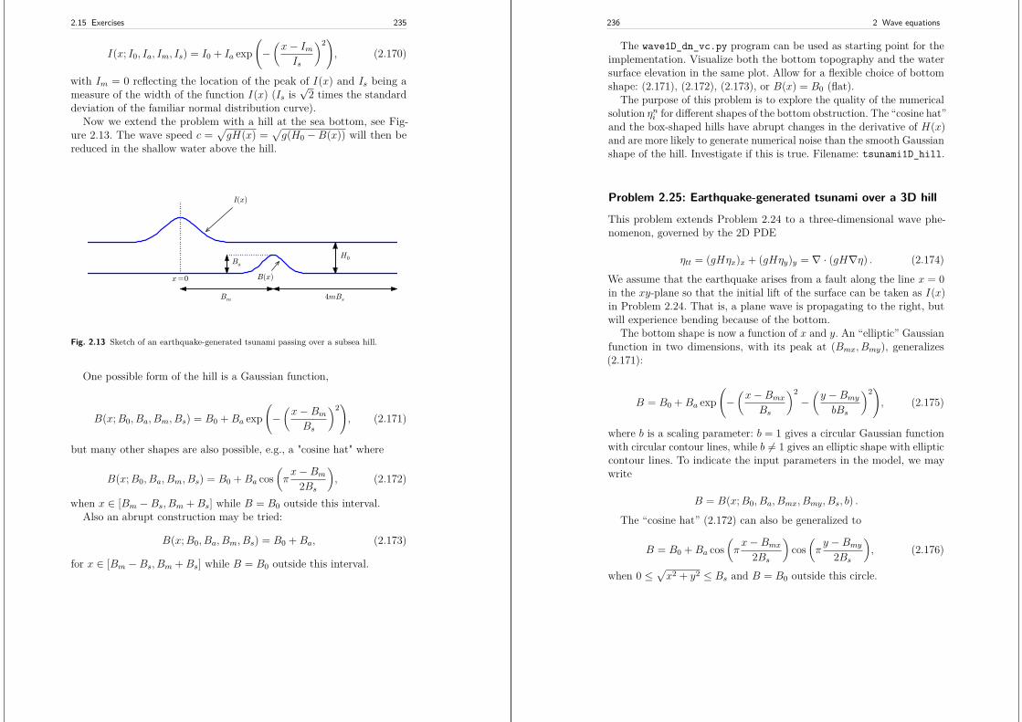
2.15 Exercises 235
I(x; I0, Ia, Im, Is) = I0 + Ia exp(−(x− ImIs
)2), (2.170)
with Im = 0 reflecting the location of the peak of I(x) and Is being ameasure of the width of the function I(x) (Is is
√2 times the standard
deviation of the familiar normal distribution curve).Now we extend the problem with a hill at the sea bottom, see Fig-
ure 2.13. The wave speed c =√gH(x) =
√g(H0 −B(x)) will then be
reduced in the shallow water above the hill.
I(x)
x=0
H0
B(x)
Ba
4mBsBm
Fig. 2.13 Sketch of an earthquake-generated tsunami passing over a subsea hill.
One possible form of the hill is a Gaussian function,
B(x;B0, Ba, Bm, Bs) = B0 +Ba exp(−(x−BmBs
)2), (2.171)
but many other shapes are also possible, e.g., a "cosine hat" where
B(x;B0, Ba, Bm, Bs) = B0 +Ba cos(πx−Bm
2Bs
), (2.172)
when x ∈ [Bm −Bs, Bm +Bs] while B = B0 outside this interval.Also an abrupt construction may be tried:
B(x;B0, Ba, Bm, Bs) = B0 +Ba, (2.173)
for x ∈ [Bm −Bs, Bm +Bs] while B = B0 outside this interval.
236 2 Wave equations
The wave1D_dn_vc.py program can be used as starting point for theimplementation. Visualize both the bottom topography and the watersurface elevation in the same plot. Allow for a flexible choice of bottomshape: (2.171), (2.172), (2.173), or B(x) = B0 (flat).
The purpose of this problem is to explore the quality of the numericalsolution ηni for different shapes of the bottom obstruction. The “cosine hat”and the box-shaped hills have abrupt changes in the derivative of H(x)and are more likely to generate numerical noise than the smooth Gaussianshape of the hill. Investigate if this is true. Filename: tsunami1D_hill.
Problem 2.25: Earthquake-generated tsunami over a 3D hill
This problem extends Problem 2.24 to a three-dimensional wave phe-nomenon, governed by the 2D PDE
ηtt = (gHηx)x + (gHηy)y = ∇ · (gH∇η) . (2.174)
We assume that the earthquake arises from a fault along the line x = 0in the xy-plane so that the initial lift of the surface can be taken as I(x)in Problem 2.24. That is, a plane wave is propagating to the right, butwill experience bending because of the bottom.
The bottom shape is now a function of x and y. An “elliptic” Gaussianfunction in two dimensions, with its peak at (Bmx, Bmy), generalizes(2.171):
B = B0 +Ba exp(−(x−BmxBs
)2−(y −BmybBs
)2), (2.175)
where b is a scaling parameter: b = 1 gives a circular Gaussian functionwith circular contour lines, while b 6= 1 gives an elliptic shape with ellipticcontour lines. To indicate the input parameters in the model, we maywrite
B = B(x;B0, Ba, Bmx, Bmy, Bs, b) .
The “cosine hat” (2.172) can also be generalized to
B = B0 +Ba cos(πx−Bmx
2Bs
)cos
(πy −Bmy
2Bs
), (2.176)
when 0 ≤√x2 + y2 ≤ Bs and B = B0 outside this circle.
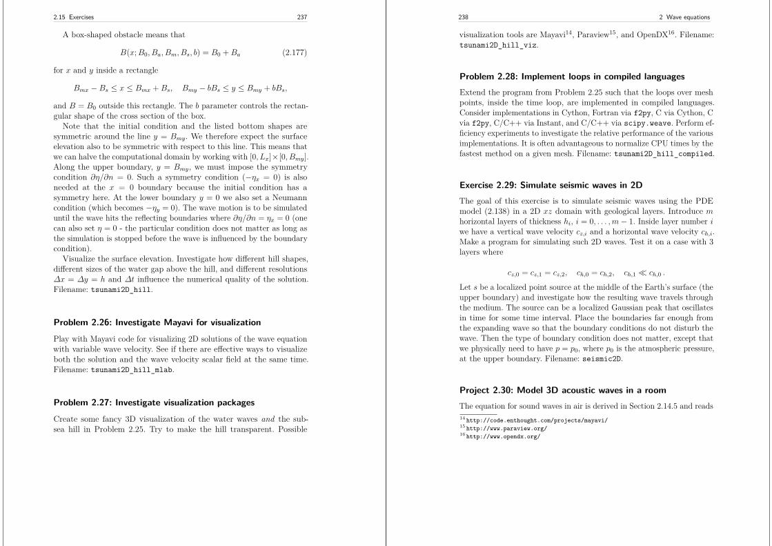
2.15 Exercises 237
A box-shaped obstacle means that
B(x;B0, Ba, Bm, Bs, b) = B0 +Ba (2.177)
for x and y inside a rectangle
Bmx −Bs ≤ x ≤ Bmx +Bs, Bmy − bBs ≤ y ≤ Bmy + bBs,
and B = B0 outside this rectangle. The b parameter controls the rectan-gular shape of the cross section of the box.
Note that the initial condition and the listed bottom shapes aresymmetric around the line y = Bmy. We therefore expect the surfaceelevation also to be symmetric with respect to this line. This means thatwe can halve the computational domain by working with [0, Lx]×[0, Bmy].Along the upper boundary, y = Bmy, we must impose the symmetrycondition ∂η/∂n = 0. Such a symmetry condition (−ηx = 0) is alsoneeded at the x = 0 boundary because the initial condition has asymmetry here. At the lower boundary y = 0 we also set a Neumanncondition (which becomes −ηy = 0). The wave motion is to be simulateduntil the wave hits the reflecting boundaries where ∂η/∂n = ηx = 0 (onecan also set η = 0 - the particular condition does not matter as long asthe simulation is stopped before the wave is influenced by the boundarycondition).
Visualize the surface elevation. Investigate how different hill shapes,different sizes of the water gap above the hill, and different resolutions∆x = ∆y = h and ∆t influence the numerical quality of the solution.Filename: tsunami2D_hill.
Problem 2.26: Investigate Mayavi for visualization
Play with Mayavi code for visualizing 2D solutions of the wave equationwith variable wave velocity. See if there are effective ways to visualizeboth the solution and the wave velocity scalar field at the same time.Filename: tsunami2D_hill_mlab.
Problem 2.27: Investigate visualization packages
Create some fancy 3D visualization of the water waves and the sub-sea hill in Problem 2.25. Try to make the hill transparent. Possible
238 2 Wave equations
visualization tools are Mayavi14, Paraview15, and OpenDX16. Filename:tsunami2D_hill_viz.
Problem 2.28: Implement loops in compiled languagesExtend the program from Problem 2.25 such that the loops over meshpoints, inside the time loop, are implemented in compiled languages.Consider implementations in Cython, Fortran via f2py, C via Cython, Cvia f2py, C/C++ via Instant, and C/C++ via scipy.weave. Perform ef-ficiency experiments to investigate the relative performance of the variousimplementations. It is often advantageous to normalize CPU times by thefastest method on a given mesh. Filename: tsunami2D_hill_compiled.
Exercise 2.29: Simulate seismic waves in 2DThe goal of this exercise is to simulate seismic waves using the PDEmodel (2.138) in a 2D xz domain with geological layers. Introduce mhorizontal layers of thickness hi, i = 0, . . . ,m− 1. Inside layer number iwe have a vertical wave velocity cz,i and a horizontal wave velocity ch,i.Make a program for simulating such 2D waves. Test it on a case with 3layers where
cz,0 = cz,1 = cz,2, ch,0 = ch,2, ch,1 ch,0 .
Let s be a localized point source at the middle of the Earth’s surface (theupper boundary) and investigate how the resulting wave travels throughthe medium. The source can be a localized Gaussian peak that oscillatesin time for some time interval. Place the boundaries far enough fromthe expanding wave so that the boundary conditions do not disturb thewave. Then the type of boundary condition does not matter, except thatwe physically need to have p = p0, where p0 is the atmospheric pressure,at the upper boundary. Filename: seismic2D.
Project 2.30: Model 3D acoustic waves in a roomThe equation for sound waves in air is derived in Section 2.14.5 and reads14 http://code.enthought.com/projects/mayavi/15 http://www.paraview.org/16 http://www.opendx.org/
2.15 Exercises 239
ptt = c2∇2p,
where p(x, y, z, t) is the pressure and c is the speed of sound, taken as 340m/s. However, sound is absorbed in the air due to relaxation of moleculesin the gas. A model for simple relaxation, valid for gases consisting onlyof one type of molecules, is a term c2τs∇2pt in the PDE, where τs is therelaxation time. If we generate sound from, e.g., a loudspeaker in theroom, this sound source must also be added to the governing equation.
The PDE with the mentioned type of damping and source then becomes
ptt = c2∇p + c2τs∇2pt + f, (2.178)
where f(x, y, z, t) is the source term.The walls can absorb some sound. A possible model is to have a
“wall layer” (thicker than the physical wall) outside the room where cis changed such that some of the wave energy is reflected and some isabsorbed in the wall. The absorption of energy can be taken care of byadding a damping term bpt in the equation:
ptt+ bpt = c2∇p + c2τs∇2pt + f . (2.179)
Typically, b = 0 in the room and b > 0 in the wall. A discontinuity in bor c will give rise to reflections. It can be wise to use a constant c in thewall to control reflections because of the discontinuity between c in theair and in the wall, while b is gradually increased as we go into the wallto avoid reflections because of rapid changes in b. At the outer boundaryof the wall the condition p = 0 or ∂p/∂n = 0 can be imposed. The wavesshould anyway be approximately dampened to p = 0 this far out in thewall layer.
There are two strategies for discretizing the ∇2pt term: using a centerdifference between times n+ 1 and n− 1 (if the equation is sampled atlevel n), or use a one-sided difference based on levels n and n− 1. Thelatter has the advantage of not leading to any equation system, whilethe former is second-order accurate as the scheme for the simple waveequation ptt = c2∇2p. To avoid an equation system, go for the one-sideddifference such that the overall scheme becomes explicit and only of firstorder in time.
Develop a 3D solver for the specified PDE and introduce a wall layer.Test the solver with the method of manufactured solutions. Make somedemonstrations where the wall reflects and absorbs the waves (reflection
240 2 Wave equations
because of discontinuity in b and absorption because of growing b).Experiment with the impact of the τs parameter. Filename: acoustics.
Project 2.31: Solve a 1D transport equationWe shall study the wave equation
ut + cux = 0, x ∈ (0, L], t ∈ (0, T ], (2.180)
with initial condition
u(x, 0) = I(x), x ∈ [0, L], (2.181)
and one periodic boundary condition
u(0, t) = u(L, t) . (2.182)
This boundary condition means that what goes out of the domain atx = L comes in at x = 0. Roughly speaking, we need only one boundarycondition because of the spatial derivative is of first order only.Physical interpretation. The parameter c can be constant or variable,c = c(x). The equation (2.180) arises in transport problems where a quan-tity u, which could be temperature or concentration of some contaminant,is transported with the velocity c of a fluid. In addition to the transportimposed by “travelling with the fluid”, u may also be transported bydiffusion (such as heat conduction or Fickian diffusion), but we have inthe model ut + cux assumed that diffusion effects are negligible, whichthey often are.a) Show that under the assumption of a = const,
u(x, t) = I(x− ct) (2.183)
fulfills the PDE as well as the initial and boundary condition (providedI(0) = I(L)).
A widely used numerical scheme for (2.180) applies a forward differencein time and a backward difference in space when c > 0:
[D+t u+ cD−x u = 0]ni . (2.184)
For c < 0 we use a forward difference in space: [cD+x u]ni .
b) Set up a computational algorithm and implement it in a function.Assume a is constant and positive.
2.15 Exercises 241
c) Test the implementation by using the remarkable property that thenumerical solution is exact at the mesh points if ∆t = c−1∆x.d) Make a movie comparing the numerical and exact solution for thefollowing two choices of initial conditions:
I(x) =[sin(πx
L
)]2n(2.185)
where n is an integer, typically n = 5, and
I(x) = exp(−(x− L/2)2
2σ2
). (2.186)
Choose ∆t = c−1∆x, 0.9c−1∆x, 0.5c−1∆x.e) The performance of the suggested numerical scheme can be investi-gated by analyzing the numerical dispersion relation. Analytically, wehave that the Fourier component
u(x, t) = ei(kx−ωt),
is a solution of the PDE if ω = kc. This is the analytical dispersionrelation. A complete solution of the PDE can be built by adding up suchFourier components with different amplitudes, where the initial conditionI determines the amplitudes. The solution u is then represented by aFourier series.
A similar discrete Fourier component at (xp, tn) is
uqp = ei(kp∆x−ωn∆t),
where in general ω is a function of k, ∆t, and ∆x, and differs from theexact ω = kc.
Insert the discrete Fourier component in the numerical scheme andderive an expression for ω, i.e., the discrete dispersion relation. Show inparticular that if ∆t/(c∆x) = 1, the discrete solution coincides with theexact solution at the mesh points, regardless of the mesh resolution (!).Show that if the stability condition
∆t
c∆x≤ 1,
the discrete Fourier component cannot grow (i.e., ω is real).f) Write a test for your implementation where you try to use informationfrom the numerical dispersion relation.
242 2 Wave equations
We shall hereafter assume that c(x) > 0.
g) Set up a computational algorithm for the variable coefficient caseand implement it in a function. Make a test that the function works forconstant a.
h) It can be shown that for an observer moving with velocity c(x), uis constant. This can be used to derive an exact solution when a varieswith x. Show first that
u(x, t) = f(C(x)− t), (2.187)
where
C ′(x) = 1c(x) ,
is a solution of (2.180) for any differentiable function f .
i) Use the initial condition to show that an exact solution is
u(x, t) = I(C−1(C(x)− t)),with C−1 being the inverse function of C =
∫c1dx. Since C(x) is an
integral∫ x
0 (1/c)dx, C(x) is monotonically increasing and there existshence an inverse function C−1 with values in [0, L].
To compute (2.187) we need to integrate 1/c to obtain C and thencompute the inverse of C.
The inverse function computation can be easily done if we first thinkdiscretely. Say we have some function y = g(x) and seek its inverse.Plotting (xi, yi), where yi = g(xi) for some mesh points xi, displays g asa function of x. The inverse function is simply x as a function of g, i.e.,the curve with points (yi, xi). We can therefore quickly compute pointsat the curve of the inverse function. One way of extending these pointsto a continuous function is to assume a linear variation (known as linearinterpolation) between the points (which actually means to draw straightlines between the points, exactly as done by a plotting program).
The function wrap2callable in scitools.std can take a set of pointsand return a continuous function that corresponds to linear variationbetween the points. The computation of the inverse of a function g on[0, L] can then be done by
def inverse(g, domain, resolution=101):x = linspace(domain[0], domain[L], resolution)y = g(x)
2.15 Exercises 243
from scitools.std import wrap2callableg_inverse = wrap2callable((y, x))return g_inverse
To compute C(x) we need to integrate 1/c, which can be done by aTrapezoidal rule. Suppose we have computed C(xi) and need to com-pute C(xi+1). Using the Trapezoidal rule with m subintervals over theintegration domain [xi, xi+1] gives
C(xi+1) = C(xi)+∫ xi+1
xi
dx
c≈ h
1
21
c(xi)+ 1
21
c(xi+1) +m−1∑
j=1
1c(xi + jh)
,
(2.188)where h = (xi+1 − xi)/m is the length of the subintervals used for theintegral over [xi, xi+1]. We observe that (2.188) is a difference equationwhich we can solve by repeatedly applying (2.188) for i = 0, 1, . . . , Nx−1if a mesh x0, x, . . . , xNx is prescribed. Note that C(0) = 0.
j) Implement a function for computing C(xi) and one for com-puting C−1(x) for any x. Use these two functions for comput-ing the exact solution I(C−1(C(x) − t)). End up with a func-tion u_exact_variable_c(x, n, c, I) that returns the value ofI(C−1(C(x)− tn)).
k) Make movies showing a comparison of the numerical and exactsolutions for the two initial conditions (2.185) and (2.31). Choose ∆t =∆x/max0,L c(x) and the velocity of the medium as
1. c(x) = 1 + ε sin(kπx/L), ε < 1,2. c(x) = 1 + I(x), where I is given by (2.185) or (2.31).
The PDE ut + cux = 0 expresses that the initial condition I(x) istransported with velocity c(x).Filename: advec1D.
Problem 2.32: General analytical solution of a 1D dampedwave equation
We consider an initial-boundary value problem for the damped waveequation:
244 2 Wave equations
utt + but = c2uxx, x ∈ (0, L), t ∈ (0, T ]u(0, t) = 0,u(L, t) = 0,u(x, 0) = I(x),ut(x, 0) = V (x) .
Here, b ≥ 0 and c are given constants. The aim is to derive a generalanalytical solution of this problem. Familiarity with the method ofseparation of variables for solving PDEs will be assumed.
a) Seek a solution on the form u(x, t) = X(x)T (t). Insert this solutionin the PDE and show that it leads to two differential equations for Xand T :
T ′′ + bT ′ + λT = 0, c2X ′′ + λX = 0,
with X(0) = X(L) = 0 as boundary conditions, and λ as a constant tobe determined.
b) Show that X(x) is on the form
Xn(x) = Cn sin kx, k = nπ
L, n = 1, 2, . . .
where Cn is an arbitrary constant.
c) Under the assumption that (b/2)2 < k2, show that T (t) is on the form
Tn(t) = e−12 bt(an cosωt+ bn sinωt), ω =
√k2 − 1
4b2, n = 1, 2, . . .
The complete solution is then
u(x, t) =∞∑
n=1sin kxe− 1
2 bt(An cosωt+Bn sinωt),
where the constants An and Bn must be computed from the initialconditions.
d) Derive a formula for An from u(x, 0) = I(x) and developing I(x) asa sine Fourier series on [0, L].
e) Derive a formula for Bn from ut(x, 0) = V (x) and developing V (x)as a sine Fourier series on [0, L].
2.15 Exercises 245
f) Calculate An and Bn from vibrations of a string where V (x) = 0 and
I(x) =ax/x0, x < x0,a(L− x)/(L− x0), otherwise (2.189)
g) Implement a function u_series(x, t, tol=1E-10) for the series foru(x, t), where tol is a tolerance for truncating the series. Simply sumthe terms until |an| and |bb| both are less than tol.
h) What will change in the derivation of the analytical solution if wehave ux(0, t) = ux(L, t) = 0 as boundary conditions? And how will yousolve the problem with u(0, t) = 0 and ux(L, t) = 0?Filename: damped_wave1D.
Problem 2.33: General analytical solution of a 2D dampedwave equation
Carry out Problem 2.32 in the 2D case: utt + but = c2(uxx + uyy), where(x, y) ∈ (0, Lx) × (0, Ly). Assume a solution on the form u(x, y, t) =X(x)Y (y)T (t). Filename: damped_wave2D.
Diffusion equations 3
The famous diffusion equation, also known as the heat equation, reads
∂u
∂t= α
∂2u
∂x2 ,
where u(x, t) is the unknown function to be solved for, x is a coordinatein space, and t is time. The coefficient α is the diffusion coefficientand determines how fast u changes in time. A quick short form for thediffusion equation is ut = αuxx.
Compared to the wave equation, utt = c2uxx, which looks very similar,the diffusion equation features solutions that are very different from thoseof the wave equation. Also, the diffusion equation makes quite differentdemands to the numerical methods.
Typical diffusion problems may experience rapid change in the verybeginning, but then the evolution of u becomes slower and slower. Thesolution is usually very smooth, and after some time, one cannot recognizethe initial shape of u. This is in sharp contrast to solutions of the waveequation where the initial shape is preserved in homogeneous media –the solution is then basically a moving initial condition. The standardwave equation utt = c2uxx has solutions that propagates with speed cforever, without changing shape, while the diffusion equation convergesto a stationary solution u(x) as t → ∞. In this limit, ut = 0, and u isgoverned by u′′(x) = 0. This stationary limit of the diffusion equation iscalled the Laplace equation and arises in a very wide range of applicationsthroughout the sciences.
© 2016, Hans Petter Langtangen, Svein Linge. Released under CC Attribution 4.0 license
248 3 Diffusion equations
It is possible to solve for u(x, t) using an explicit scheme, as we doin Section 3.1, but the time step restrictions soon become much lessfavorable than for an explicit scheme applied to the wave equation. Andof more importance, since the solution u of the diffusion equation isvery smooth and changes slowly, small time steps are not convenientand not required by accuracy as the diffusion process converges to astationary state. Therefore, implicit schemes (as described in Section 3.2)are popular, but these require solutions of systems of algebraic equations.We shall use ready-made software for this purpose, but also programsome simple iterative methods. The exposition is, as usual in this book,very basic and focuses on the basic ideas and how to implement. Morecomprehensive mathematical treatments and classical analysis of themethods are found in lots of textbooks. A favorite of ours in this respectis the one by LeVeque [13]. The books by Strikwerda [17] and by Lapidusand Pinder [12] are also highly recommended as additional material onthe topic.
3.1 An explicit method for the 1D diffusion equation
Explicit finite difference methods for the wave equation utt = c2uxx canbe used, with small modifications, for solving ut = αuxx as well. Theexposition below assumes that the reader is familiar with the basic ideasof discretization and implementation of wave equations from Chapter 2.Readers not familiar with the Forward Euler, Backward Euler, and Crank-Nicolson (or centered or midpoint) discretization methods in time shouldconsult, e.g., Section 1.1 in [9].
3.1.1 The initial-boundary value problem for 1D diffusionTo obtain a unique solution of the diffusion equation, or equivalently, toapply numerical methods, we need initial and boundary conditions. Thediffusion equation goes with one initial condition u(x, 0) = I(x), whereI is a prescribed function. One boundary condition is required at eachpoint on the boundary, which in 1D means that u must be known, uxmust be known, or some combination of them.
We shall start with the simplest boundary condition: u = 0. Thecomplete initial-boundary value diffusion problem in one space dimensioncan then be specified as
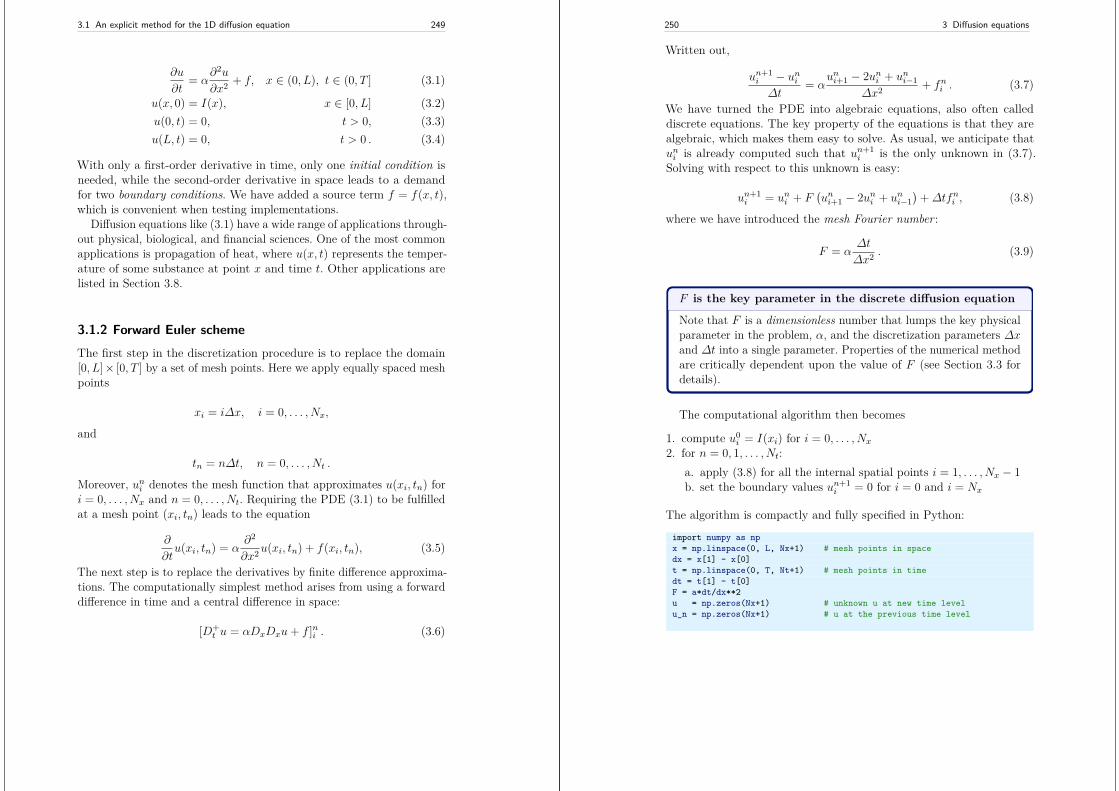
3.1 An explicit method for the 1D diffusion equation 249
∂u
∂t= α
∂2u
∂x2 + f, x ∈ (0, L), t ∈ (0, T ] (3.1)
u(x, 0) = I(x), x ∈ [0, L] (3.2)u(0, t) = 0, t > 0, (3.3)u(L, t) = 0, t > 0 . (3.4)
With only a first-order derivative in time, only one initial condition isneeded, while the second-order derivative in space leads to a demandfor two boundary conditions. We have added a source term f = f(x, t),which is convenient when testing implementations.
Diffusion equations like (3.1) have a wide range of applications through-out physical, biological, and financial sciences. One of the most commonapplications is propagation of heat, where u(x, t) represents the temper-ature of some substance at point x and time t. Other applications arelisted in Section 3.8.
3.1.2 Forward Euler schemeThe first step in the discretization procedure is to replace the domain[0, L]× [0, T ] by a set of mesh points. Here we apply equally spaced meshpoints
xi = i∆x, i = 0, . . . , Nx,
and
tn = n∆t, n = 0, . . . , Nt .
Moreover, uni denotes the mesh function that approximates u(xi, tn) fori = 0, . . . , Nx and n = 0, . . . , Nt. Requiring the PDE (3.1) to be fulfilledat a mesh point (xi, tn) leads to the equation
∂
∂tu(xi, tn) = α
∂2
∂x2u(xi, tn) + f(xi, tn), (3.5)
The next step is to replace the derivatives by finite difference approxima-tions. The computationally simplest method arises from using a forwarddifference in time and a central difference in space:
[D+t u = αDxDxu+ f ]ni . (3.6)
250 3 Diffusion equations
Written out,
un+1i − uni∆t
= αuni+1 − 2uni + uni−1
∆x2 + fni . (3.7)
We have turned the PDE into algebraic equations, also often calleddiscrete equations. The key property of the equations is that they arealgebraic, which makes them easy to solve. As usual, we anticipate thatuni is already computed such that un+1
i is the only unknown in (3.7).Solving with respect to this unknown is easy:
un+1i = uni + F
(uni+1 − 2uni + uni−1
)+∆tfni , (3.8)
where we have introduced the mesh Fourier number :
F = α∆t
∆x2 . (3.9)
F is the key parameter in the discrete diffusion equation
Note that F is a dimensionless number that lumps the key physicalparameter in the problem, α, and the discretization parameters ∆xand ∆t into a single parameter. Properties of the numerical methodare critically dependent upon the value of F (see Section 3.3 fordetails).
The computational algorithm then becomes
1. compute u0i = I(xi) for i = 0, . . . , Nx
2. for n = 0, 1, . . . , Nt:a. apply (3.8) for all the internal spatial points i = 1, . . . , Nx − 1b. set the boundary values un+1
i = 0 for i = 0 and i = Nx
The algorithm is compactly and fully specified in Python:
import numpy as npx = np.linspace(0, L, Nx+1) # mesh points in spacedx = x[1] - x[0]t = np.linspace(0, T, Nt+1) # mesh points in timedt = t[1] - t[0]F = a*dt/dx**2u = np.zeros(Nx+1) # unknown u at new time levelu_n = np.zeros(Nx+1) # u at the previous time level
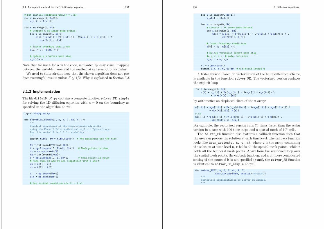
3.1 An explicit method for the 1D diffusion equation 251
# Set initial condition u(x,0) = I(x)for i in range(0, Nx+1):
u_n[i] = I(x[i])
for n in range(0, Nt):# Compute u at inner mesh pointsfor i in range(1, Nx):
u[i] = u_n[i] + F*(u_n[i-1] - 2*u_n[i] + u_n[i+1]) + \dt*f(x[i], t[n])
# Insert boundary conditionsu[0] = 0; u[Nx] = 0
# Update u_n before next stepu_n[:]= u
Note that we use a for α in the code, motivated by easy visual mappingbetween the variable name and the mathematical symbol in formulas.
We need to state already now that the shown algorithm does not pro-duce meaningful results unless F ≤ 1/2. Why is explained in Section 3.3.
3.1.3 ImplementationThe file diffu1D_u0.py contains a complete function solver_FE_simplefor solving the 1D diffusion equation with u = 0 on the boundary asspecified in the algorithm above:
import numpy as np
def solver_FE_simple(I, a, f, L, dt, F, T):"""Simplest expression of the computational algorithmusing the Forward Euler method and explicit Python loops.For this method F <= 0.5 for stability."""import time; t0 = time.clock() # For measuring the CPU time
Nt = int(round(T/float(dt)))t = np.linspace(0, Nt*dt, Nt+1) # Mesh points in timedx = np.sqrt(a*dt/F)Nx = int(round(L/dx))x = np.linspace(0, L, Nx+1) # Mesh points in space# Make sure dx and dt are compatible with x and tdx = x[1] - x[0]dt = t[1] - t[0]
u = np.zeros(Nx+1)u_n = np.zeros(Nx+1)
# Set initial condition u(x,0) = I(x)
252 3 Diffusion equations
for i in range(0, Nx+1):u_n[i] = I(x[i])
for n in range(0, Nt):# Compute u at inner mesh pointsfor i in range(1, Nx):
u[i] = u_n[i] + F*(u_n[i-1] - 2*u_n[i] + u_n[i+1]) + \dt*f(x[i], t[n])
# Insert boundary conditionsu[0] = 0; u[Nx] = 0
# Switch variables before next step#u_n[:] = u # safe, but slowu_n, u = u, u_n
t1 = time.clock()return u_n, x, t, t1-t0 # u_n holds latest u
A faster version, based on vectorization of the finite difference scheme,is available in the function solver_FE. The vectorized version replacesthe explicit loop
for i in range(1, Nx):u[i] = u_n[i] + F*(u_n[i-1] - 2*u_n[i] + u_n[i+1]) \
+ dt*f(x[i], t[n])
by arithmetics on displaced slices of the u array:
u[1:Nx] = u_n[1:Nx] + F*(u_n[0:Nx-1] - 2*u_n[1:Nx] + u_n[2:Nx+1]) \+ dt*f(x[1:Nx], t[n])
# oru[1:-1] = u_n[1:-1] + F*(u_n[0:-2] - 2*u_n[1:-1] + u_n[2:]) \
+ dt*f(x[1:-1], t[n])
For example, the vectorized version runs 70 times faster than the scalarversion in a case with 100 time steps and a spatial mesh of 105 cells.
The solver_FE function also features a callback function such thatthe user can process the solution at each time level. The callback functionlooks like user_action(u, x, t, n), where u is the array containingthe solution at time level n, x holds all the spatial mesh points, while tholds all the temporal mesh points. Apart from the vectorized loop overthe spatial mesh points, the callback function, and a bit more complicatedsetting of the source f it is not specified (None), the solver_FE functionis identical to solver_FE_simple above:
def solver_FE(I, a, f, L, dt, F, T,user_action=None, version=’scalar’):
"""Vectorized implementation of solver_FE_simple."""
3.1 An explicit method for the 1D diffusion equation 253
import time; t0 = time.clock() # for measuring the CPU time
Nt = int(round(T/float(dt)))t = np.linspace(0, Nt*dt, Nt+1) # Mesh points in timedx = np.sqrt(a*dt/F)Nx = int(round(L/dx))x = np.linspace(0, L, Nx+1) # Mesh points in space# Make sure dx and dt are compatible with x and tdx = x[1] - x[0]dt = t[1] - t[0]
u = np.zeros(Nx+1) # solution arrayu_n = np.zeros(Nx+1) # solution at t-dt
# Set initial conditionfor i in range(0,Nx+1):
u_n[i] = I(x[i])
if user_action is not None:user_action(u_n, x, t, 0)
for n in range(0, Nt):# Update all inner pointsif version == ’scalar’:
for i in range(1, Nx):u[i] = u_n[i] +\
F*(u_n[i-1] - 2*u_n[i] + u_n[i+1]) +\dt*f(x[i], t[n])
elif version == ’vectorized’:u[1:Nx] = u_n[1:Nx] + \
F*(u_n[0:Nx-1] - 2*u_n[1:Nx] + u_n[2:Nx+1]) +\dt*f(x[1:Nx], t[n])
else:raise ValueError(’version=%s’ % version)
# Insert boundary conditionsu[0] = 0; u[Nx] = 0if user_action is not None:
user_action(u, x, t, n+1)
# Switch variables before next stepu_n, u = u, u_n
t1 = time.clock()return t1-t0
3.1.4 VerificationExact solution of discrete equations. Before thinking about runningthe functions in the previous section, we need to construct a suitable test
254 3 Diffusion equations
example for verification. It appears that a manufactured solution that islinear in time and at most quadratic in space fulfills the Forward Eulerscheme exactly. With the restriction that u = 0 for x = 0, L, we can trythe solution
u(x, t) = 5tx(L− x) .
Inserted in the PDE, it requires a source term
f(x, t) = 10αt+ 5x(L− x) .
With the formulas from Appendix A.4 we can easily check that themanufactured u fulfills the scheme:
[D+t u = αDxDxu+ f ]ni = [5x(L− x)D+
t t = 5tαDxDx(xL− x2)+10αt+ 5x(L− x)]ni
= [5x(L− x) = 5tα(−2) + 10αt+ 5x(L− x)]ni ,
which is a 0=0 expression. The computation of the source term, givenany u, is easily automated with sympy:
import sympy as symx, t, a, L = sym.symbols(’x t a L’)u = x*(L-x)*5*t
def pde(u):return sym.diff(u, t) - a*sym.diff(u, x, x)
f = sym.simplify(pde(u))
Now we can choose any expression for u and automatically get thesuitable source term f. However, the manufactured solution u will ingeneral not be exactly reproduced by the scheme: only constant andlinear functions are differentiated correctly by a forward difference, whileonly constant, linear, and quadratic functions are differentiated exactlyby a [DxDxu]ni difference.
The numerical code will need to access the u and f above asPython functions. The exact solution is wanted as a Python functionu_exact(x, t), while the source term is wanted as f(x, t). The pa-rameters a and L in u and f above are symbols and must be replacedby float objects in a Python function. This can be done by redefininga and L as float objects and performing substitutions of symbols bynumbers in u and f. The appropriate code looks like this:
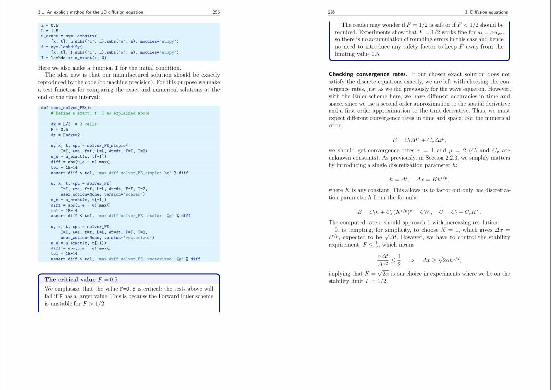
3.1 An explicit method for the 1D diffusion equation 255
a = 0.5L = 1.5u_exact = sym.lambdify(
[x, t], u.subs(’L’, L).subs(’a’, a), modules=’numpy’)f = sym.lambdify(
[x, t], f.subs(’L’, L).subs(’a’, a), modules=’numpy’)I = lambda x: u_exact(x, 0)
Here we also make a function I for the initial condition.The idea now is that our manufactured solution should be exactly
reproduced by the code (to machine precision). For this purpose we makea test function for comparing the exact and numerical solutions at theend of the time interval:
def test_solver_FE():# Define u_exact, f, I as explained above
dx = L/3 # 3 cellsF = 0.5dt = F*dx**2
u, x, t, cpu = solver_FE_simple(I=I, a=a, f=f, L=L, dt=dt, F=F, T=2)
u_e = u_exact(x, t[-1])diff = abs(u_e - u).max()tol = 1E-14assert diff < tol, ’max diff solver_FE_simple: %g’ % diff
u, x, t, cpu = solver_FE(I=I, a=a, f=f, L=L, dt=dt, F=F, T=2,user_action=None, version=’scalar’)
u_e = u_exact(x, t[-1])diff = abs(u_e - u).max()tol = 1E-14assert diff < tol, ’max diff solver_FE, scalar: %g’ % diff
u, x, t, cpu = solver_FE(I=I, a=a, f=f, L=L, dt=dt, F=F, T=2,user_action=None, version=’vectorized’)
u_e = u_exact(x, t[-1])diff = abs(u_e - u).max()tol = 1E-14assert diff < tol, ’max diff solver_FE, vectorized: %g’ % diff
The critical value F = 0.5We emphasize that the value F=0.5 is critical: the tests above willfail if F has a larger value. This is because the Forward Euler schemeis unstable for F > 1/2.
256 3 Diffusion equations
The reader may wonder if F = 1/2 is safe or if F < 1/2 should berequired. Experiments show that F = 1/2 works fine for ut = αuxx,so there is no accumulation of rounding errors in this case and henceno need to introduce any safety factor to keep F away from thelimiting value 0.5.
Checking convergence rates. If our chosen exact solution does notsatisfy the discrete equations exactly, we are left with checking the con-vergence rates, just as we did previously for the wave equation. However,with the Euler scheme here, we have different accuracies in time andspace, since we use a second order approximation to the spatial derivativeand a first order approximation to the time derivative. Thus, we mustexpect different convergence rates in time and space. For the numericalerror,
E = Ct∆tr + Cx∆x
p,
we should get convergence rates r = 1 and p = 2 (Ct and Cx areunknown constants). As previously, in Section 2.2.3, we simplify mattersby introducing a single discretization parameter h:
h = ∆t, ∆x = Khr/p,
where K is any constant. This allows us to factor out only one discretiza-tion parameter h from the formula:
E = Cth+ Cx(Kr/p)p = Chr, C = Ct + CsKr .
The computed rate r should approach 1 with increasing resolution.It is tempting, for simplicity, to choose K = 1, which gives ∆x =
hr/p, expected to be√∆t. However, we have to control the stability
requirement: F ≤ 12 , which means
α∆t
∆x2 ≤12 ⇒ ∆x ≥
√2αh1/2,
implying that K =√
2α is our choice in experiments where we lie on thestability limit F = 1/2.
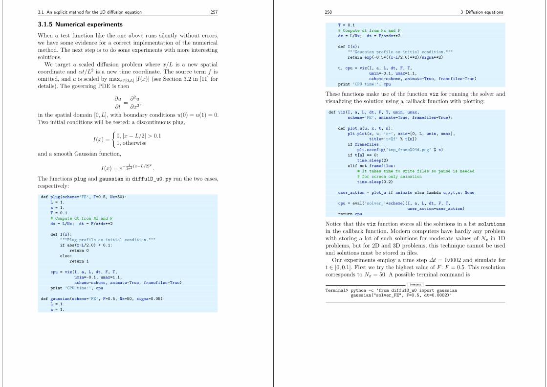
3.1 An explicit method for the 1D diffusion equation 257
3.1.5 Numerical experimentsWhen a test function like the one above runs silently without errors,we have some evidence for a correct implementation of the numericalmethod. The next step is to do some experiments with more interestingsolutions.
We target a scaled diffusion problem where x/L is a new spatialcoordinate and αt/L2 is a new time coordinate. The source term f isomitted, and u is scaled by maxx∈[0,L] |I(x)| (see Section 3.2 in [11] fordetails). The governing PDE is then
∂u
∂t= ∂2u
∂x2 ,
in the spatial domain [0, L], with boundary conditions u(0) = u(1) = 0.Two initial conditions will be tested: a discontinuous plug,
I(x) =
0, |x− L/2| > 0.11, otherwise
and a smooth Gaussian function,
I(x) = e−1
2σ2 (x−L/2)2.
The functions plug and gaussian in diffu1D_u0.py run the two cases,respectively:
def plug(scheme=’FE’, F=0.5, Nx=50):L = 1.a = 1.T = 0.1# Compute dt from Nx and Fdx = L/Nx; dt = F/a*dx**2
def I(x):"""Plug profile as initial condition."""if abs(x-L/2.0) > 0.1:
return 0else:
return 1
cpu = viz(I, a, L, dt, F, T,umin=-0.1, umax=1.1,scheme=scheme, animate=True, framefiles=True)
print ’CPU time:’, cpu
def gaussian(scheme=’FE’, F=0.5, Nx=50, sigma=0.05):L = 1.a = 1.
258 3 Diffusion equations
T = 0.1# Compute dt from Nx and Fdx = L/Nx; dt = F/a*dx**2
def I(x):"""Gaussian profile as initial condition."""return exp(-0.5*((x-L/2.0)**2)/sigma**2)
u, cpu = viz(I, a, L, dt, F, T,umin=-0.1, umax=1.1,scheme=scheme, animate=True, framefiles=True)
print ’CPU time:’, cpu
These functions make use of the function viz for running the solver andvisualizing the solution using a callback function with plotting:
def viz(I, a, L, dt, F, T, umin, umax,scheme=’FE’, animate=True, framefiles=True):
def plot_u(u, x, t, n):plt.plot(x, u, ’r-’, axis=[0, L, umin, umax],
title=’t=%f’ % t[n])if framefiles:
plt.savefig(’tmp_frame%04d.png’ % n)if t[n] == 0:
time.sleep(2)elif not framefiles:
# It takes time to write files so pause is needed# for screen only animationtime.sleep(0.2)
user_action = plot_u if animate else lambda u,x,t,n: None
cpu = eval(’solver_’+scheme)(I, a, L, dt, F, T,user_action=user_action)
return cpu
Notice that this viz function stores all the solutions in a list solutionsin the callback function. Modern computers have hardly any problemwith storing a lot of such solutions for moderate values of Nx in 1Dproblems, but for 2D and 3D problems, this technique cannot be usedand solutions must be stored in files.
Our experiments employ a time step ∆t = 0.0002 and simulate fort ∈ [0, 0.1]. First we try the highest value of F : F = 0.5. This resolutioncorresponds to Nx = 50. A possible terminal command is
Terminal
Terminal> python -c ’from diffu1D_u0 import gaussiangaussian("solver_FE", F=0.5, dt=0.0002)’
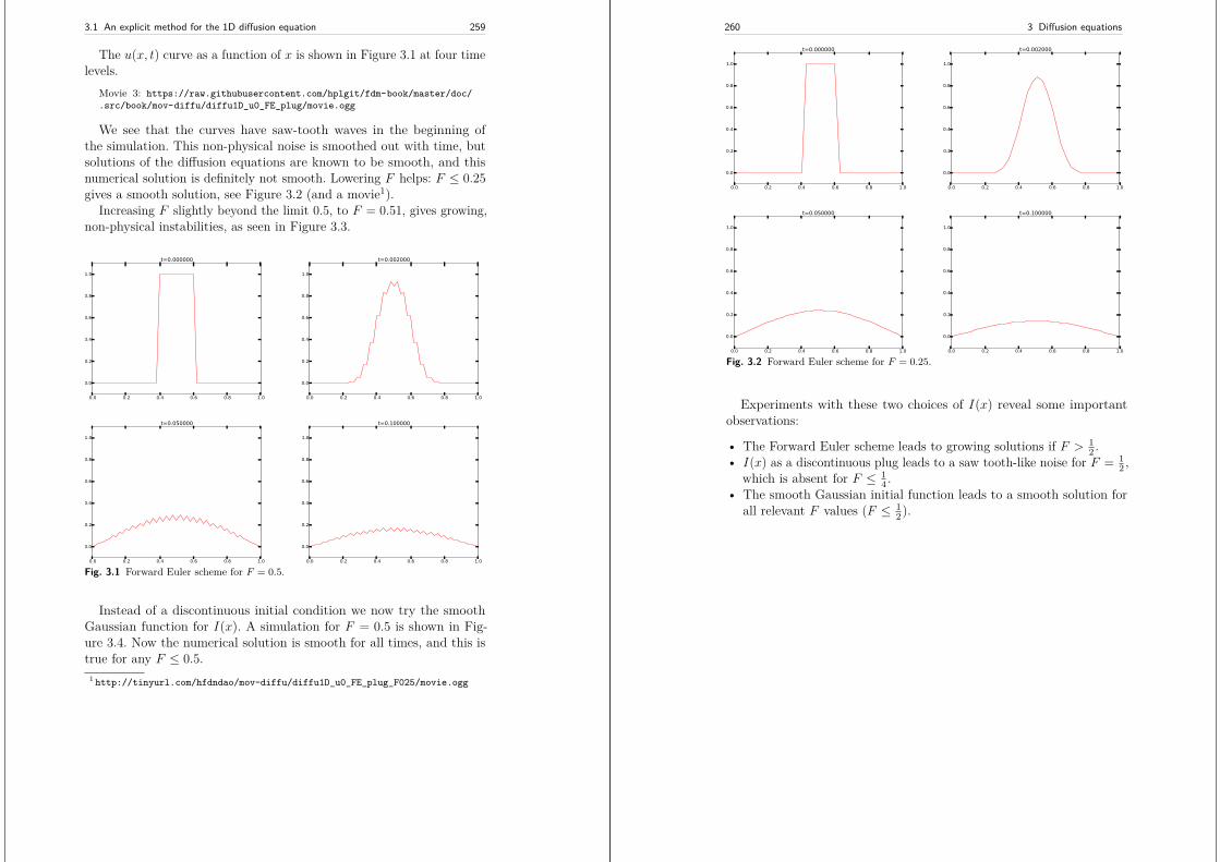
3.1 An explicit method for the 1D diffusion equation 259
The u(x, t) curve as a function of x is shown in Figure 3.1 at four timelevels.
Movie 3: https://raw.githubusercontent.com/hplgit/fdm-book/master/doc/.src/book/mov-diffu/diffu1D_u0_FE_plug/movie.ogg
We see that the curves have saw-tooth waves in the beginning ofthe simulation. This non-physical noise is smoothed out with time, butsolutions of the diffusion equations are known to be smooth, and thisnumerical solution is definitely not smooth. Lowering F helps: F ≤ 0.25gives a smooth solution, see Figure 3.2 (and a movie1).
Increasing F slightly beyond the limit 0.5, to F = 0.51, gives growing,non-physical instabilities, as seen in Figure 3.3.
0.0 0.2 0.4 0.6 0.8 1.0
0.0
0.2
0.4
0.6
0.8
1.0
t=0.000000
0.0 0.2 0.4 0.6 0.8 1.0
0.0
0.2
0.4
0.6
0.8
1.0
t=0.002000
0.0 0.2 0.4 0.6 0.8 1.0
0.0
0.2
0.4
0.6
0.8
1.0
t=0.050000
0.0 0.2 0.4 0.6 0.8 1.0
0.0
0.2
0.4
0.6
0.8
1.0
t=0.100000
Fig. 3.1 Forward Euler scheme for F = 0.5.
Instead of a discontinuous initial condition we now try the smoothGaussian function for I(x). A simulation for F = 0.5 is shown in Fig-ure 3.4. Now the numerical solution is smooth for all times, and this istrue for any F ≤ 0.5.
1 http://tinyurl.com/hfdndao/mov-diffu/diffu1D_u0_FE_plug_F025/movie.ogg
260 3 Diffusion equations
0.0 0.2 0.4 0.6 0.8 1.0
0.0
0.2
0.4
0.6
0.8
1.0
t=0.000000
0.0 0.2 0.4 0.6 0.8 1.0
0.0
0.2
0.4
0.6
0.8
1.0
t=0.002000
0.0 0.2 0.4 0.6 0.8 1.0
0.0
0.2
0.4
0.6
0.8
1.0
t=0.050000
0.0 0.2 0.4 0.6 0.8 1.0
0.0
0.2
0.4
0.6
0.8
1.0
t=0.100000
Fig. 3.2 Forward Euler scheme for F = 0.25.
Experiments with these two choices of I(x) reveal some importantobservations:
• The Forward Euler scheme leads to growing solutions if F > 12 .
• I(x) as a discontinuous plug leads to a saw tooth-like noise for F = 12 ,
which is absent for F ≤ 14 .
• The smooth Gaussian initial function leads to a smooth solution forall relevant F values (F ≤ 1
2).
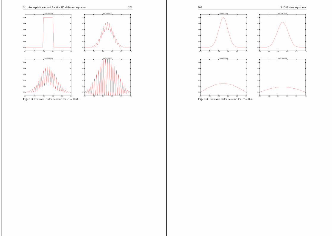
3.1 An explicit method for the 1D diffusion equation 261
0.0 0.2 0.4 0.6 0.8 1.0
0.0
0.2
0.4
0.6
0.8
1.0
t=0.000000
0.0 0.2 0.4 0.6 0.8 1.0
0.0
0.2
0.4
0.6
0.8
1.0
t=0.005000
0.0 0.2 0.4 0.6 0.8 1.0
0.0
0.2
0.4
0.6
0.8
1.0
t=0.010000
0.0 0.2 0.4 0.6 0.8 1.0
0.0
0.2
0.4
0.6
0.8
1.0
t=0.015000
Fig. 3.3 Forward Euler scheme for F = 0.51.
262 3 Diffusion equations
0.0 0.2 0.4 0.6 0.8 1.0
0.0
0.2
0.4
0.6
0.8
1.0
t=0.000000
0.0 0.2 0.4 0.6 0.8 1.0
0.0
0.2
0.4
0.6
0.8
1.0
t=0.002000
0.0 0.2 0.4 0.6 0.8 1.0
0.0
0.2
0.4
0.6
0.8
1.0
t=0.050000
0.0 0.2 0.4 0.6 0.8 1.0
0.0
0.2
0.4
0.6
0.8
1.0
t=0.100000
Fig. 3.4 Forward Euler scheme for F = 0.5.
3.2 Implicit methods for the 1D diffusion equation 263
3.2 Implicit methods for the 1D diffusion equation
Simulations with the Forward Euler scheme shows that the time steprestriction, F ≤ 1
2 , which means ∆t ≤ ∆x2/(2α), may be relevant in thebeginning of the diffusion process, when the solution changes quite fast,but as time increases, the process slows down, and a small ∆t may beinconvenient. By using implicit schemes, which lead to coupled systemsof linear equations to be solved at each time level, any size of ∆t ispossible (but the accuracy decreases with increasing ∆t). The BackwardEuler scheme, derived and implemented below, is the simplest implicitscheme for the diffusion equation.
3.2.1 Backward Euler scheme
We now apply a backward difference in time in (3.5), but the same centraldifference in space:
[D−t u = DxDxu+ f ]ni , (3.10)
which written out reads
uni − un−1i
∆t= α
uni+1 − 2uni + uni−1∆x2 + fni . (3.11)
Now we assume un−1i is already computed, but all quantities at the
“new” time level n are unknown. This time it is not possible to solvewith respect to uni because this value couples to its neighbors in space,uni−1 and uni+1, which are also unknown. Let us examine this fact for thecase when Nx = 3. Equation (3.11) written for i = 1, . . . , Nx− 1 = 1, 2becomes
un1 − un−11
∆t= α
un2 − 2un1 + un0∆x2 + fn1 (3.12)
un2 − un−12
∆t= α
un3 − 2un2 + un1∆x2 + fn2 (3.13)
The boundary values un0 and un3 are known as zero. Collecting the un-known new values un1 and un2 on the left-hand side and multiplying by∆t gives
264 3 Diffusion equations
(1 + 2F )un1 − Fun2 = un−11 +∆tfn1 , (3.14)
−Fun1 + (1 + 2F )un2 = un−12 +∆tfn2 . (3.15)
This is a coupled 2× 2 system of algebraic equations for the unknownsun1 and un2 . The equivalent matrix form is
(1 + 2F −F−F 1 + 2F
)(un1un2
)=(un−1
1 +∆tfn1un−1
2 +∆tfn2
)
Terminology: implicit vs. explicit methods
Discretization methods that lead to a coupled system of equationsfor the unknown function at a new time level are said to be implicitmethods. The counterpart, explicit methods, refers to discretizationmethods where there is a simple explicit formula for the values ofthe unknown function at each of the spatial mesh points at thenew time level. From an implementational point of view, implicitmethods are more comprehensive to code since they require thesolution of coupled equations, i.e., a matrix system, at each timelevel. With explicit methods we have a closed-form formula for thevalue of the unknown at each mesh point.
Very often explicit schemes have a restriction on the size of thetime step that can be relaxed by using implicit schemes. In fact,implicit schemes are frequently unconditionally stable, so the sizeof the time step is governed by accuracy and not by stability. Thisis the great advantage of implicit schemes.
In the general case, (3.11) gives rise to a coupled (Nx − 1)× (Nx − 1)system of algebraic equations for all the unknown uni at the interior spatialpoints i = 1, . . . , Nx − 1. Collecting the unknowns on the left-hand side,(3.11) can be written
− Funi−1 + (1 + 2F )uni − Funi+1 = un−1i−1 , (3.16)
for i = 1, . . . , Nx − 1. One can either view these equations as a systemfor where the uni values at the internal mesh points, i = 1, . . . , Nx − 1,are unknown, or we may append the boundary values un0 and unNx to thesystem. In the latter case, all uni for i = 0, . . . , Nx are considered unknown,and we must add the boundary equations to the Nx − 1 equations in(3.16):
3.2 Implicit methods for the 1D diffusion equation 265
un0 = 0, (3.17)unNx = 0 . (3.18)
A coupled system of algebraic equations can be written on matrixform, and this is important if we want to call up ready-made software forsolving the system. The equations (3.16) and (3.17)–(3.18) correspondto the matrix equation
AU = b
where U = (un0 , . . . , unNx), and the matrix A has the following structure:
A =
A0,0 A0,1 0 · · · · · · · · · · · · · · · 0A1,0 A1,1 A1,2
. . . ...0 A2,1 A2,2 A2,3
. . . ...... . . . . . . . . . 0
...... . . . . . . . . . . . . . . . ...... 0 Ai,i−1 Ai,i Ai,i+1
. . . ...... . . . . . . . . . . . . 0... . . . . . . . . . ANx−1,Nx0 · · · · · · · · · · · · · · · 0 ANx,Nx−1 ANx,Nx
(3.19)The nonzero elements are given by
Ai,i−1 = −F (3.20)Ai,i = 1 + 2F (3.21)
Ai,i+1 = −F (3.22)
in the equations for internal points, i = 1, . . . , Nx − 1. The first andlast equation correspond to the boundary condition, where we know thesolution, and therefore we must have
266 3 Diffusion equations
A0,0 = 1, (3.23)A0,1 = 0, (3.24)
ANx,Nx−1 = 0, (3.25)ANx,Nx = 1 . (3.26)
The right-hand side b is written as
b =
b0b1...bi...bNx
(3.27)
with
b0 = 0, (3.28)bi = un−1
i , i = 1, . . . , Nx − 1, (3.29)bNx = 0 . (3.30)
We observe that the matrix A contains quantities that do not changein time. Therefore, A can be formed once and for all before we enterthe recursive formulas for the time evolution. The right-hand side b,however, must be updated at each time step. This leads to the followingcomputational algorithm, here sketched with Python code:
x = np.linspace(0, L, Nx+1) # mesh points in spacedx = x[1] - x[0]t = np.linspace(0, T, N+1) # mesh points in timeu = np.zeros(Nx+1) # unknown u at new time levelu_n = np.zeros(Nx+1) # u at the previous time level
# Data structures for the linear systemA = np.zeros((Nx+1, Nx+1))b = np.zeros(Nx+1)
for i in range(1, Nx):A[i,i-1] = -FA[i,i+1] = -FA[i,i] = 1 + 2*F
A[0,0] = A[Nx,Nx] = 1
# Set initial condition u(x,0) = I(x)
3.2 Implicit methods for the 1D diffusion equation 267
for i in range(0, Nx+1):u_n[i] = I(x[i])
import scipy.linalg
for n in range(0, Nt):# Compute b and solve linear systemfor i in range(1, Nx):
b[i] = -u_n[i]b[0] = b[Nx] = 0u[:] = scipy.linalg.solve(A, b)
# Update u_n before next stepu_n[:] = u
Regarding verification, the same considerations apply as for the For-ward Euler method (Section 3.1.4).
3.2.2 Sparse matrix implementation
We have seen from (3.19) that the matrix A is tridiagonal. The codesegment above used a full, dense matrix representation of A, which storesa lot of values we know are zero beforehand, and worse, the solutionalgorithm computes with all these zeros. With Nx+1 unknowns, the workby the solution algorithm is 1
3(Nx + 1)3 and the storage requirements(Nx + 1)2. By utilizing the fact that A is tridiagonal and employingcorresponding software tools that work with the three diagonals, thework and storage demands can be proportional to Nx only. This leads toa dramatic improvement: with Nx = 200, which is a realistic resolution,the code runs about 40,000 times faster and reduces the storage to just1.5%! It is no doubt that we should take advantage of the fact that A istridiagonal.
The key idea is to apply a data structure for a tridiagonal or sparsematrix. The scipy.sparse package has relevant utilities. For example,we can store only the nonzero diagonals of a matrix. The package alsohas linear system solvers that operate on sparse matrix data structures.The code below illustrates how we can store only the main diagonal andthe upper and lower diagonals.
# Representation of sparse matrix and right-hand sidemain = np.zeros(Nx+1)lower = np.zeros(Nx)upper = np.zeros(Nx)b = np.zeros(Nx+1)
268 3 Diffusion equations
# Precompute sparse matrixmain[:] = 1 + 2*Flower[:] = -Fupper[:] = -F# Insert boundary conditionsmain[0] = 1main[Nx] = 1
A = scipy.sparse.diags(diagonals=[main, lower, upper],offsets=[0, -1, 1], shape=(Nx+1, Nx+1),format=’csr’)
print A.todense() # Check that A is correct
# Set initial conditionfor i in range(0,Nx+1):
u_n[i] = I(x[i])
for n in range(0, Nt):b = u_nb[0] = b[-1] = 0.0 # boundary conditionsu[:] = scipy.sparse.linalg.spsolve(A, b)u_n[:] = u
The scipy.sparse.linalg.spsolve function utilizes the sparse storagestructure of A and performs, in this case, a very efficient Gaussianelimination solve.
The program diffu1D_u0.py contains a function solver_BE, whichimplements the Backward Euler scheme sketched above. As mentioned inSection 3.1.2, the functions plug and gaussian runs the case with I(x)as a discontinuous plug or a smooth Gaussian function. All experimentspoint to two characteristic features of the Backward Euler scheme: 1) itis always stable, and 2) it always gives a smooth, decaying solution.
3.2.3 Crank-Nicolson schemeThe idea in the Crank-Nicolson scheme is to apply centered differencesin space and time, combined with an average in time. We demand thePDE to be fulfilled at the spatial mesh points, but midway between thepoints in the time mesh:
∂
∂tu(xi, tn+ 1
2) = α
∂2
∂x2u(xi, tn+ 12) + f(xi, tn+ 1
2),
for i = 1, . . . , Nx − 1 and n = 0, . . . , Nt − 1.With centered differences in space and time, we get
3.2 Implicit methods for the 1D diffusion equation 269
[Dtu = αDxDxu+ f ]n+ 12
i .
On the right-hand side we get an expression
1∆x2
(un+ 1
2i−1 − 2un+ 1
2i + u
n+ 12
i+1
)+ f
n+ 12
i .
This expression is problematic since un+ 12
i is not one of the unknowns wecompute. A possibility is to replace un+ 1
2i by an arithmetic average:
un+ 1
2i ≈ 1
2(uni + un+1
i
).
In the compact notation, we can use the arithmetic average notation ut:
[Dtu = αDxDxut + f ]n+ 1
2i .
We can also use an average for fn+ 12
i :
[Dtu = αDxDxut + f
t]n+ 12
i .
After writing out the differences and average, multiplying by ∆t, andcollecting all unknown terms on the left-hand side, we get
un+1i − 1
2F (un+1i−1 − 2un+1
i + un+1i+1 ) = uni + 1
2F (uni−1 − 2uni + uni+1)12f
n+1i + 1
2fni . (3.31)
Also here, as in the Backward Euler scheme, the new unknowns un+1i−1 ,
un+1i , and un+1
i+1 are coupled in a linear system AU = b, where A has thesame structure as in (3.19), but with slightly different entries:
Ai,i−1 = −12F (3.32)
Ai,i = 1 + F (3.33)
Ai,i+1 = −12F (3.34)
in the equations for internal points, i = 1, . . . , Nx − 1. The equations forthe boundary points correspond to
270 3 Diffusion equations
A0,0 = 1, (3.35)A0,1 = 0, (3.36)
ANx,Nx−1 = 0, (3.37)ANx,Nx = 1 . (3.38)
The right-hand side b has entries
b0 = 0, (3.39)
bi = un−1i + 1
2(fni + fn+1i ), i = 1, . . . , Nx − 1, (3.40)
bNx = 0 . (3.41)
When verifying some implementation of the Crank-Nicolson schemeby convergence rate testing, one should note that the scheme is secondorder accurate in both space and time. The numerical error then reads
E = Ct∆tr + Cx∆x
r,
where r = 2 (Ct and Cx are unknown constants, as before). Whenintroducing a single discretization parameter, we may now simply choose
h = ∆x = ∆t,
which givesE = Cth
r + Cxhr = (Ct + Cx)hr,
where r should approach 2 as resolution is increased in the convergencerate computations.
3.2.4 The unifying θ rule
For the equation
∂u
∂t= G(u),
where G(u) is some spatial differential operator, the θ-rule looks like
un+1i − uni∆t
= θG(un+1i ) + (1− θ)G(uni ) .
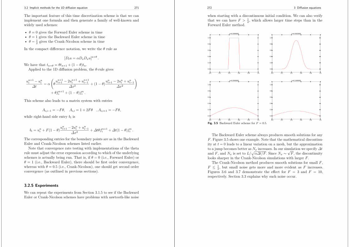
3.2 Implicit methods for the 1D diffusion equation 271
The important feature of this time discretization scheme is that we canimplement one formula and then generate a family of well-known andwidely used schemes:
• θ = 0 gives the Forward Euler scheme in time• θ = 1 gives the Backward Euler scheme in time• θ = 1
2 gives the Crank-Nicolson scheme in time
In the compact difference notation, we write the θ rule as
[Dtu = αDxDxu]n+θ .
We have that tn+θ = θtn+1 + (1− θ)tn.Applied to the 1D diffusion problem, the θ-rule gives
un+1i − uni∆t
= α
(θun+1i+1 − 2un+1
i + un+1i−1
∆x2 + (1− θ)uni+1 − 2uni + uni−1
∆x2
)
+ θfn+1i + (1− θ)fni .
This scheme also leads to a matrix system with entries
Ai,i−1 = −Fθ, Ai,i = 1 + 2Fθ ,Ai,i+1 = −Fθ,while right-hand side entry bi is
bi = uni + F (1− θ)uni+1 − 2uni + uni−1
∆x2 +∆tθfn+1i +∆t(1− θ)fni .
The corresponding entries for the boundary points are as in the BackwardEuler and Crank-Nicolson schemes listed earlier.
Note that convergence rate testing with implementations of the thetarule must adjust the error expression according to which of the underlyingschemes is actually being run. That is, if θ = 0 (i.e., Forward Euler) orθ = 1 (i.e., Backward Euler), there should be first order convergence,whereas with θ = 0.5 (i.e., Crank-Nicolson), one should get second orderconvergence (as outlined in previous sections).
3.2.5 ExperimentsWe can repeat the experiments from Section 3.1.5 to see if the BackwardEuler or Crank-Nicolson schemes have problems with sawtooth-like noise
272 3 Diffusion equations
when starting with a discontinuous initial condition. We can also verifythat we can have F > 1
2 , which allows larger time steps than in theForward Euler method.
0.0 0.2 0.4 0.6 0.8 1.0
0.0
0.2
0.4
0.6
0.8
1.0
t=0.000000
0.0 0.2 0.4 0.6 0.8 1.0
0.0
0.2
0.4
0.6
0.8
1.0
t=0.002000
0.0 0.2 0.4 0.6 0.8 1.0
0.0
0.2
0.4
0.6
0.8
1.0
t=0.050000
0.0 0.2 0.4 0.6 0.8 1.0
0.0
0.2
0.4
0.6
0.8
1.0
t=0.100000
Fig. 3.5 Backward Euler scheme for F = 0.5.
The Backward Euler scheme always produces smooth solutions for anyF . Figure 3.5 shows one example. Note that the mathematical discontinu-ity at t = 0 leads to a linear variation on a mesh, but the approximationto a jump becomes better as Nx increases. In our simulation we specify ∆tand F , and Nx is set to L/
√α∆t/F . Since Nx ∼
√F , the discontinuity
looks sharper in the Crank-Nicolson simulations with larger F .The Crank-Nicolson method produces smooth solutions for small F ,
F ≤ 12 , but small noise gets more and more evident as F increases.
Figures 3.6 and 3.7 demonstrate the effect for F = 3 and F = 10,respectively. Section 3.3 explains why such noise occur.
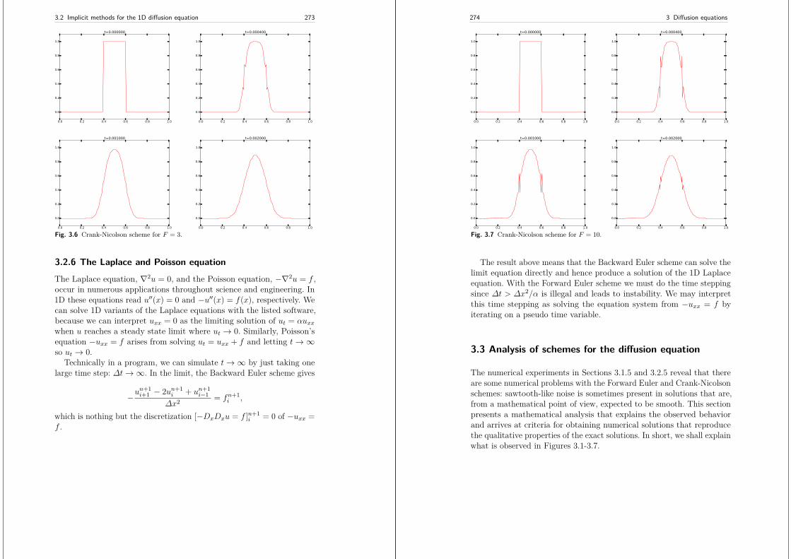
3.2 Implicit methods for the 1D diffusion equation 273
0.0 0.2 0.4 0.6 0.8 1.0
0.0
0.2
0.4
0.6
0.8
1.0
t=0.000000
0.0 0.2 0.4 0.6 0.8 1.0
0.0
0.2
0.4
0.6
0.8
1.0
t=0.000400
0.0 0.2 0.4 0.6 0.8 1.0
0.0
0.2
0.4
0.6
0.8
1.0
t=0.001000
0.0 0.2 0.4 0.6 0.8 1.0
0.0
0.2
0.4
0.6
0.8
1.0
t=0.002000
Fig. 3.6 Crank-Nicolson scheme for F = 3.
3.2.6 The Laplace and Poisson equation
The Laplace equation, ∇2u = 0, and the Poisson equation, −∇2u = f ,occur in numerous applications throughout science and engineering. In1D these equations read u′′(x) = 0 and −u′′(x) = f(x), respectively. Wecan solve 1D variants of the Laplace equations with the listed software,because we can interpret uxx = 0 as the limiting solution of ut = αuxxwhen u reaches a steady state limit where ut → 0. Similarly, Poisson’sequation −uxx = f arises from solving ut = uxx + f and letting t→∞so ut → 0.
Technically in a program, we can simulate t→∞ by just taking onelarge time step: ∆t→∞. In the limit, the Backward Euler scheme gives
−un+1i+1 − 2un+1
i + un+1i−1
∆x2 = fn+1i ,
which is nothing but the discretization [−DxDxu = f ]n+1i = 0 of −uxx =
f .
274 3 Diffusion equations
0.0 0.2 0.4 0.6 0.8 1.0
0.0
0.2
0.4
0.6
0.8
1.0
t=0.000000
0.0 0.2 0.4 0.6 0.8 1.0
0.0
0.2
0.4
0.6
0.8
1.0
t=0.000400
0.0 0.2 0.4 0.6 0.8 1.0
0.0
0.2
0.4
0.6
0.8
1.0
t=0.001000
0.0 0.2 0.4 0.6 0.8 1.0
0.0
0.2
0.4
0.6
0.8
1.0
t=0.002000
Fig. 3.7 Crank-Nicolson scheme for F = 10.
The result above means that the Backward Euler scheme can solve thelimit equation directly and hence produce a solution of the 1D Laplaceequation. With the Forward Euler scheme we must do the time steppingsince ∆t > ∆x2/α is illegal and leads to instability. We may interpretthis time stepping as solving the equation system from −uxx = f byiterating on a pseudo time variable.
3.3 Analysis of schemes for the diffusion equation
The numerical experiments in Sections 3.1.5 and 3.2.5 reveal that thereare some numerical problems with the Forward Euler and Crank-Nicolsonschemes: sawtooth-like noise is sometimes present in solutions that are,from a mathematical point of view, expected to be smooth. This sectionpresents a mathematical analysis that explains the observed behaviorand arrives at criteria for obtaining numerical solutions that reproducethe qualitative properties of the exact solutions. In short, we shall explainwhat is observed in Figures 3.1-3.7.
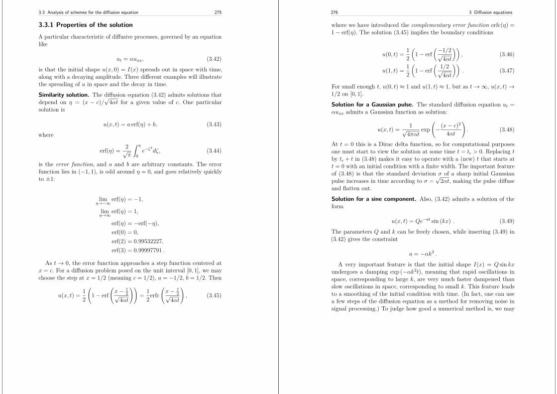
3.3 Analysis of schemes for the diffusion equation 275
3.3.1 Properties of the solution
A particular characteristic of diffusive processes, governed by an equationlike
ut = αuxx, (3.42)
is that the initial shape u(x, 0) = I(x) spreads out in space with time,along with a decaying amplitude. Three different examples will illustratethe spreading of u in space and the decay in time.
Similarity solution. The diffusion equation (3.42) admits solutions thatdepend on η = (x − c)/
√4αt for a given value of c. One particular
solution is
u(x, t) = a erf(η) + b, (3.43)
where
erf(η) = 2√π
∫ η
0e−ζ
2dζ, (3.44)
is the error function, and a and b are arbitrary constants. The errorfunction lies in (−1, 1), is odd around η = 0, and goes relatively quicklyto ±1:
limη→−∞
erf(η) = −1,
limη→∞
erf(η) = 1,
erf(η) = −erf(−η),erf(0) = 0,erf(2) = 0.99532227,erf(3) = 0.99997791 .
As t→ 0, the error function approaches a step function centered atx = c. For a diffusion problem posed on the unit interval [0, 1], we maychoose the step at x = 1/2 (meaning c = 1/2), a = −1/2, b = 1/2. Then
u(x, t) = 12
(1− erf
(x− 1
2√4αt
))= 1
2erfc(x− 1
2√4αt
), (3.45)
276 3 Diffusion equations
where we have introduced the complementary error function erfc(η) =1− erf(η). The solution (3.45) implies the boundary conditions
u(0, t) = 12
(1− erf
(−1/2√4αt
)), (3.46)
u(1, t) = 12
(1− erf
( 1/2√4αt
)). (3.47)
For small enough t, u(0, t) ≈ 1 and u(1, t) ≈ 1, but as t→∞, u(x, t)→1/2 on [0, 1].
Solution for a Gaussian pulse. The standard diffusion equation ut =αuxx admits a Gaussian function as solution:
u(x, t) = 1√4παt
exp(−(x− c)2
4αt
). (3.48)
At t = 0 this is a Dirac delta function, so for computational purposesone must start to view the solution at some time t = tε > 0. Replacing tby tε + t in (3.48) makes it easy to operate with a (new) t that starts att = 0 with an initial condition with a finite width. The important featureof (3.48) is that the standard deviation σ of a sharp initial Gaussianpulse increases in time according to σ =
√2αt, making the pulse diffuse
and flatten out.
Solution for a sine component. Also, (3.42) admits a solution of theform
u(x, t) = Qe−at sin (kx) . (3.49)
The parameters Q and k can be freely chosen, while inserting (3.49) in(3.42) gives the constraint
a = −αk2 .
A very important feature is that the initial shape I(x) = Q sin kxundergoes a damping exp (−αk2t), meaning that rapid oscillations inspace, corresponding to large k, are very much faster dampened thanslow oscillations in space, corresponding to small k. This feature leadsto a smoothing of the initial condition with time. (In fact, one can usea few steps of the diffusion equation as a method for removing noise insignal processing.) To judge how good a numerical method is, we may
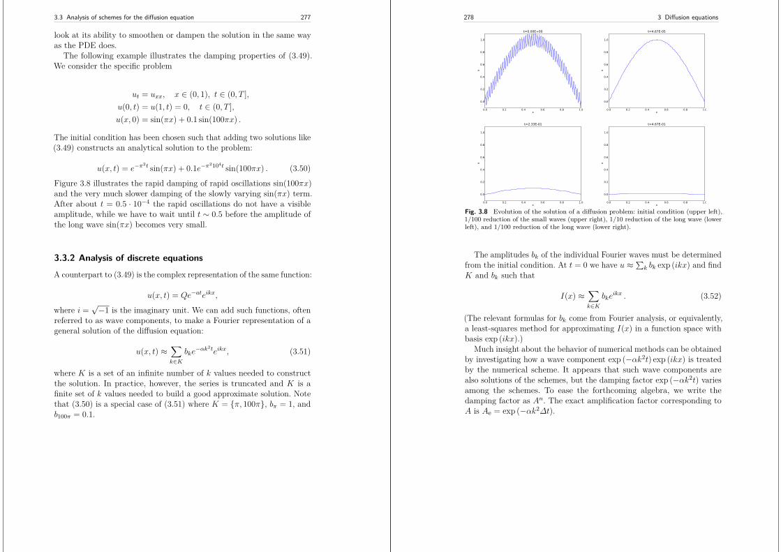
3.3 Analysis of schemes for the diffusion equation 277
look at its ability to smoothen or dampen the solution in the same wayas the PDE does.
The following example illustrates the damping properties of (3.49).We consider the specific problem
ut = uxx, x ∈ (0, 1), t ∈ (0, T ],u(0, t) = u(1, t) = 0, t ∈ (0, T ],u(x, 0) = sin(πx) + 0.1 sin(100πx) .
The initial condition has been chosen such that adding two solutions like(3.49) constructs an analytical solution to the problem:
u(x, t) = e−π2t sin(πx) + 0.1e−π2104t sin(100πx) . (3.50)
Figure 3.8 illustrates the rapid damping of rapid oscillations sin(100πx)and the very much slower damping of the slowly varying sin(πx) term.After about t = 0.5 · 10−4 the rapid oscillations do not have a visibleamplitude, while we have to wait until t ∼ 0.5 before the amplitude ofthe long wave sin(πx) becomes very small.
3.3.2 Analysis of discrete equations
A counterpart to (3.49) is the complex representation of the same function:
u(x, t) = Qe−ateikx,
where i =√−1 is the imaginary unit. We can add such functions, often
referred to as wave components, to make a Fourier representation of ageneral solution of the diffusion equation:
u(x, t) ≈∑
k∈Kbke−αk2teikx, (3.51)
where K is a set of an infinite number of k values needed to constructthe solution. In practice, however, the series is truncated and K is afinite set of k values needed to build a good approximate solution. Notethat (3.50) is a special case of (3.51) where K = π, 100π, bπ = 1, andb100π = 0.1.
278 3 Diffusion equations
0.0 0.2 0.4 0.6 0.8 1.0x
0.0
0.2
0.4
0.6
0.8
1.0
u
t=0.00E+00
0.0 0.2 0.4 0.6 0.8 1.0x
0.0
0.2
0.4
0.6
0.8
1.0
u
t=4.67E-05
0.0 0.2 0.4 0.6 0.8 1.0x
0.0
0.2
0.4
0.6
0.8
1.0
u
t=2.33E-01
0.0 0.2 0.4 0.6 0.8 1.0x
0.0
0.2
0.4
0.6
0.8
1.0
u
t=4.67E-01
Fig. 3.8 Evolution of the solution of a diffusion problem: initial condition (upper left),1/100 reduction of the small waves (upper right), 1/10 reduction of the long wave (lowerleft), and 1/100 reduction of the long wave (lower right).
The amplitudes bk of the individual Fourier waves must be determinedfrom the initial condition. At t = 0 we have u ≈∑k bk exp (ikx) and findK and bk such that
I(x) ≈∑
k∈Kbke
ikx . (3.52)
(The relevant formulas for bk come from Fourier analysis, or equivalently,a least-squares method for approximating I(x) in a function space withbasis exp (ikx).)
Much insight about the behavior of numerical methods can be obtainedby investigating how a wave component exp (−αk2t) exp (ikx) is treatedby the numerical scheme. It appears that such wave components arealso solutions of the schemes, but the damping factor exp (−αk2t) variesamong the schemes. To ease the forthcoming algebra, we write thedamping factor as An. The exact amplification factor corresponding toA is Ae = exp (−αk2∆t).
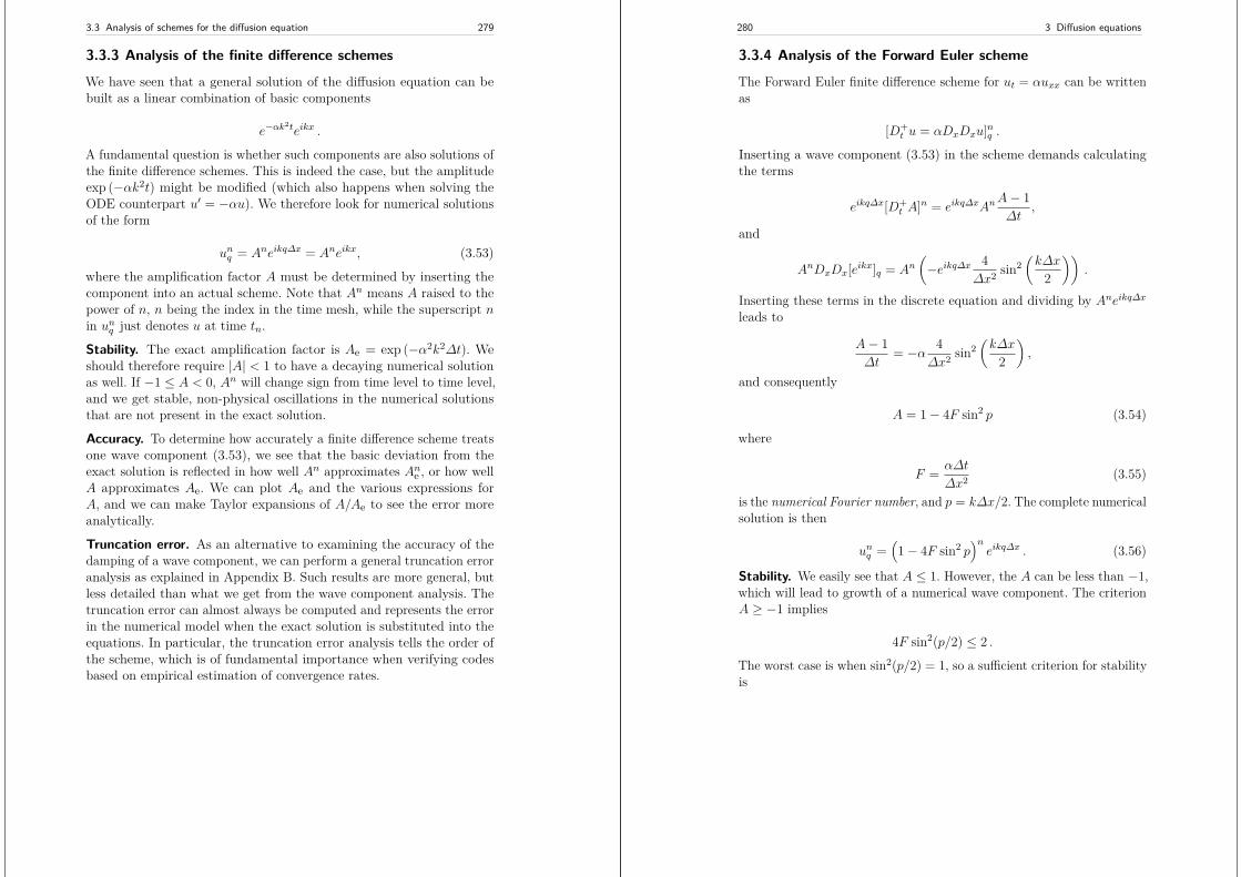
3.3 Analysis of schemes for the diffusion equation 279
3.3.3 Analysis of the finite difference schemes
We have seen that a general solution of the diffusion equation can bebuilt as a linear combination of basic components
e−αk2teikx .
A fundamental question is whether such components are also solutions ofthe finite difference schemes. This is indeed the case, but the amplitudeexp (−αk2t) might be modified (which also happens when solving theODE counterpart u′ = −αu). We therefore look for numerical solutionsof the form
unq = Aneikq∆x = Aneikx, (3.53)
where the amplification factor A must be determined by inserting thecomponent into an actual scheme. Note that An means A raised to thepower of n, n being the index in the time mesh, while the superscript nin unq just denotes u at time tn.
Stability. The exact amplification factor is Ae = exp (−α2k2∆t). Weshould therefore require |A| < 1 to have a decaying numerical solutionas well. If −1 ≤ A < 0, An will change sign from time level to time level,and we get stable, non-physical oscillations in the numerical solutionsthat are not present in the exact solution.
Accuracy. To determine how accurately a finite difference scheme treatsone wave component (3.53), we see that the basic deviation from theexact solution is reflected in how well An approximates Ane , or how wellA approximates Ae. We can plot Ae and the various expressions forA, and we can make Taylor expansions of A/Ae to see the error moreanalytically.
Truncation error. As an alternative to examining the accuracy of thedamping of a wave component, we can perform a general truncation erroranalysis as explained in Appendix B. Such results are more general, butless detailed than what we get from the wave component analysis. Thetruncation error can almost always be computed and represents the errorin the numerical model when the exact solution is substituted into theequations. In particular, the truncation error analysis tells the order ofthe scheme, which is of fundamental importance when verifying codesbased on empirical estimation of convergence rates.
280 3 Diffusion equations
3.3.4 Analysis of the Forward Euler scheme
The Forward Euler finite difference scheme for ut = αuxx can be writtenas
[D+t u = αDxDxu]nq .
Inserting a wave component (3.53) in the scheme demands calculatingthe terms
eikq∆x[D+t A]n = eikq∆xAn
A− 1∆t
,
and
AnDxDx[eikx]q = An(−eikq∆x 4
∆x2 sin2(k∆x
2
)).
Inserting these terms in the discrete equation and dividing by Aneikq∆xleads to
A− 1∆t
= −α 4∆x2 sin2
(k∆x
2
),
and consequently
A = 1− 4F sin2 p (3.54)
where
F = α∆t
∆x2 (3.55)
is the numerical Fourier number, and p = k∆x/2. The complete numericalsolution is then
unq =(1− 4F sin2 p
)neikq∆x . (3.56)
Stability. We easily see that A ≤ 1. However, the A can be less than −1,which will lead to growth of a numerical wave component. The criterionA ≥ −1 implies
4F sin2(p/2) ≤ 2 .
The worst case is when sin2(p/2) = 1, so a sufficient criterion for stabilityis
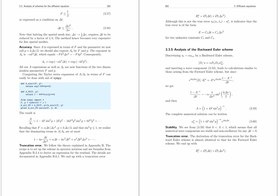
3.3 Analysis of schemes for the diffusion equation 281
F ≤ 12 , (3.57)
or expressed as a condition on ∆t:
∆t ≤ ∆x2
2α . (3.58)
Note that halving the spatial mesh size, ∆x→ 12∆x, requires ∆t to be
reduced by a factor of 1/4. The method hence becomes very expensivefor fine spatial meshes.Accuracy. Since A is expressed in terms of F and the parameter we nowcall p = k∆x/2, we should also express Ae by F and p. The exponent inAe is −αk2∆t, which equals −Fk2∆x2 = −F4p2. Consequently,
Ae = exp (−αk2∆t) = exp (−4Fp2) .
All our A expressions as well as Ae are now functions of the two dimen-sionless parameters F and p.
Computing the Taylor series expansion of A/Ae in terms of F caneasily be done with aid of sympy:
def A_exact(F, p):return exp(-4*F*p**2)
def A_FE(F, p):return 1 - 4*F*sin(p)**2
from sympy import *F, p = symbols(’F p’)A_err_FE = A_FE(F, p)/A_exact(F, p)print A_err_FE.series(F, 0, 6)
The result is
A
Ae= 1− 4F sin2 p+ 2Fp2 − 16F 2p2 sin2 p+ 8F 2p4 + · · ·
Recalling that F = α∆t/∆x2, p = k∆x/2, and that sin2 p ≤ 1, we realizethat the dominating terms in A/Ae are at most
1− 4α ∆t
∆x2 + α∆t− 4α2∆t2 + α2∆t2∆x2 + · · · .
Truncation error. We follow the theory explained in Appendix B. Therecipe is to set up the scheme in operator notation and use formulas fromAppendix B.2.4 to derive an expression for the residual. The details aredocumented in Appendix B.6.1. We end up with a truncation error
282 3 Diffusion equations
Rni = O(∆t) +O(∆x2) .
Although this is not the true error ue(xi, tn)− uni , it indicates that thetrue error is of the form
E = Ct∆t+ Cx∆x2
for two unknown constants Ct and Cx.
3.3.5 Analysis of the Backward Euler scheme
Discretizing ut = αuxx by a Backward Euler scheme,
[D−t u = αDxDxu]nq ,
and inserting a wave component (3.53), leads to calculations similar tothose arising from the Forward Euler scheme, but since
eikq∆x[D−t A]n = Aneikq∆x1− A−1
∆t,
we get
1− A−1
∆t= −α 4
∆x2 sin2(k∆x
2
),
and then
A =(1 + 4F sin2 p
)−1. (3.59)
The complete numerical solution can be written
unq =(1 + 4F sin2 p
)−neikq∆x . (3.60)
Stability. We see from (3.59) that 0 < A < 1, which means that allnumerical wave components are stable and non-oscillatory for any ∆t > 0.
Truncation error. The derivation of the truncation error for the Back-ward Euler scheme is almost identical to that for the Forward Eulerscheme. We end up with
Rni = O(∆t) +O(∆x2) .
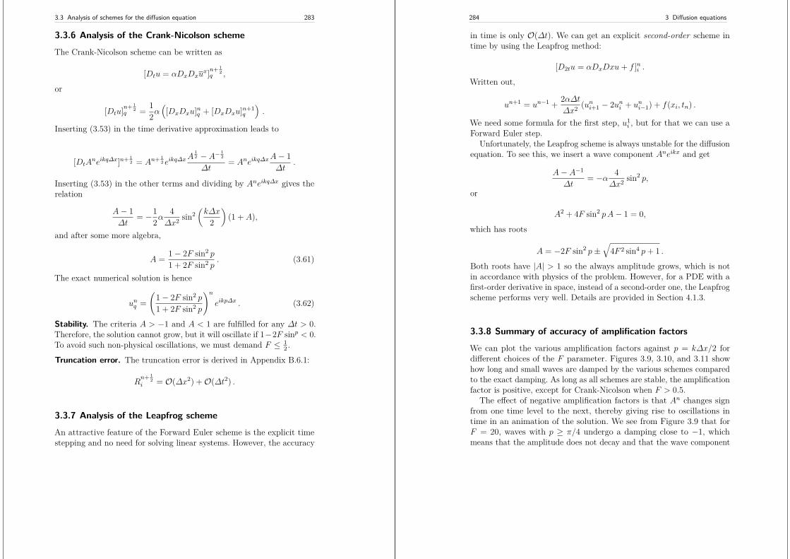
3.3 Analysis of schemes for the diffusion equation 283
3.3.6 Analysis of the Crank-Nicolson scheme
The Crank-Nicolson scheme can be written as
[Dtu = αDxDxux]n+ 1
2q ,
or
[Dtu]n+ 12
q = 12α([DxDxu]nq + [DxDxu]n+1
q
).
Inserting (3.53) in the time derivative approximation leads to
[DtAneikq∆x]n+ 1
2 = An+ 12 eikq∆x
A12 − A− 1
2
∆t= Aneikq∆x
A− 1∆t
.
Inserting (3.53) in the other terms and dividing by Aneikq∆x gives therelation
A− 1∆t
= −12α
4∆x2 sin2
(k∆x
2
)(1 + A),
and after some more algebra,
A = 1− 2F sin2 p
1 + 2F sin2 p. (3.61)
The exact numerical solution is hence
unq =(
1− 2F sin2 p
1 + 2F sin2 p
)neikp∆x . (3.62)
Stability. The criteria A > −1 and A < 1 are fulfilled for any ∆t > 0.Therefore, the solution cannot grow, but it will oscillate if 1−2F sinp < 0.To avoid such non-physical oscillations, we must demand F ≤ 1
2 .
Truncation error. The truncation error is derived in Appendix B.6.1:
Rn+ 1
2i = O(∆x2) +O(∆t2) .
3.3.7 Analysis of the Leapfrog scheme
An attractive feature of the Forward Euler scheme is the explicit timestepping and no need for solving linear systems. However, the accuracy
284 3 Diffusion equations
in time is only O(∆t). We can get an explicit second-order scheme intime by using the Leapfrog method:
[D2tu = αDxDxu+ f ]ni .
Written out,
un+1 = un−1 + 2α∆t∆x2 (uni+1 − 2uni + uni−1) + f(xi, tn) .
We need some formula for the first step, u1i , but for that we can use a
Forward Euler step.Unfortunately, the Leapfrog scheme is always unstable for the diffusion
equation. To see this, we insert a wave component Aneikx and get
A− A−1
∆t= −α 4
∆x2 sin2 p,
or
A2 + 4F sin2 pA− 1 = 0,
which has roots
A = −2F sin2 p±√
4F 2 sin4 p+ 1 .
Both roots have |A| > 1 so the always amplitude grows, which is notin accordance with physics of the problem. However, for a PDE with afirst-order derivative in space, instead of a second-order one, the Leapfrogscheme performs very well. Details are provided in Section 4.1.3.
3.3.8 Summary of accuracy of amplification factors
We can plot the various amplification factors against p = k∆x/2 fordifferent choices of the F parameter. Figures 3.9, 3.10, and 3.11 showhow long and small waves are damped by the various schemes comparedto the exact damping. As long as all schemes are stable, the amplificationfactor is positive, except for Crank-Nicolson when F > 0.5.
The effect of negative amplification factors is that An changes signfrom one time level to the next, thereby giving rise to oscillations intime in an animation of the solution. We see from Figure 3.9 that forF = 20, waves with p ≥ π/4 undergo a damping close to −1, whichmeans that the amplitude does not decay and that the wave component
3.3 Analysis of schemes for the diffusion equation 285
0.0 0.2 0.4 0.6 0.8 1.0 1.2 1.4p=k∆x
1.0
0.5
0.0
0.5
1.0
A(p
)
F=20
BEexactCNFE
0.0 0.2 0.4 0.6 0.8 1.0 1.2 1.4p=k∆x
1.0
0.5
0.0
0.5
1.0
A(p
)
F=2
BEexactCNFE
Fig. 3.9 Amplification factors for large time steps.
0.0 0.2 0.4 0.6 0.8 1.0 1.2 1.4p=k∆x
1.0
0.5
0.0
0.5
1.0
A(p
)
F=0.5
BEexactCNFE
0.0 0.2 0.4 0.6 0.8 1.0 1.2 1.4p=k∆x
1.0
0.5
0.0
0.5
1.0
A(p
)
F=0.25
BEexactCNFE
Fig. 3.10 Amplification factors for time steps around the Forward Euler stability limit.
0.0 0.2 0.4 0.6 0.8 1.0 1.2 1.4p=k∆x
0.3
0.4
0.5
0.6
0.7
0.8
0.9
1.0
A(p
)
F=0.1
BEexactCNFE
0.0 0.2 0.4 0.6 0.8 1.0 1.2 1.4p=k∆x
0.75
0.80
0.85
0.90
0.95
1.00
A(p
)
F=0.01
BEexactCNFE
Fig. 3.11 Amplification factors for small time steps.
jumps up and down (flips amplitude) in time. For F = 2 we have adamping of a factor of 0.5 from one time level to the next, which is verymuch smaller than the exact damping. Short waves will therefore fail tobe effectively dampened. These waves will manifest themselves as highfrequency oscillatory noise in the solution.
A value p = π/4 corresponds to four mesh points per wave length ofeikx, while p = π/2 implies only two points per wave length, which isthe smallest number of points we can have to represent the wave on themesh.
286 3 Diffusion equations
To demonstrate the oscillatory behavior of the Crank-Nicolson scheme,we choose an initial condition that leads to short waves with significantamplitude. A discontinuous I(x) will in particular serve this purpose:Figures 3.6 and 3.7 correspond to F = 3 and F = 10, respectively, andwe see how short waves pollute the overall solution.
3.3.9 Analysis of the 2D diffusion equation
We first consider the 2D diffusion equation
ut = α(uxx + uyy),
which has Fourier component solutions of the form
u(x, y, t) = Ae−αk2tei(kxx+kyy),
and the schemes have discrete versions of this Fourier component:
unq,r = Aξnei(kxq∆x+kyr∆y) .
The Forward Euler scheme. For the Forward Euler discretization,
[D+t u = α(DxDxu+DyDyu)]ni,j ,
we get
ξ − 1∆t
= −α 4∆x2 sin2
(kx∆x
2
)− α 4
∆y2 sin2(ky∆y
2
).
Introducing
px = kx∆x
2 , py = ky∆y
2 ,
we can write the equation for ξ more compactly as
ξ − 1∆t
= −α 4∆x2 sin2 px − α
4∆y2 sin2 py,
and solve for ξ:
ξ = 1− 4Fx sin2 px − 4Fy sin2 py . (3.63)
The complete numerical solution for a wave component is
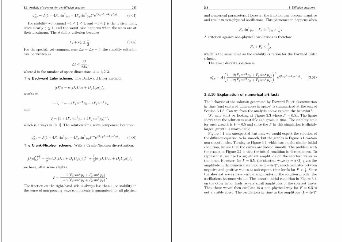
3.3 Analysis of schemes for the diffusion equation 287
unq,r = A(1− 4Fx sin2 px − 4Fy sin2 py)nei(kxp∆x+kyq∆y) . (3.64)
For stability we demand −1 ≤ ξ ≤ 1, and −1 ≤ ξ is the critical limit,since clearly ξ ≤ 1, and the worst case happens when the sines are attheir maximum. The stability criterion becomes
Fx + Fy ≤12 . (3.65)
For the special, yet common, case ∆x = ∆y = h, the stability criterioncan be written as
∆t ≤ h2
2dα,
where d is the number of space dimensions: d = 1, 2, 3.
The Backward Euler scheme. The Backward Euler method,
[D−t u = α(DxDxu+DyDyu)]ni,j ,
results in
1− ξ−1 = −4Fx sin2 px − 4Fy sin2 py,
and
ξ = (1 + 4Fx sin2 px + 4Fy sin2 py)−1,
which is always in (0, 1]. The solution for a wave component becomes
unq,r = A(1 + 4Fx sin2 px + 4Fy sin2 py)−nei(kxq∆x+kyr∆y) . (3.66)
The Crank-Nicolson scheme. With a Crank-Nicolson discretization,
[Dtu]n+ 12
i,j = 12[α(DxDxu+DyDyu)]n+1
i,j + 12[α(DxDxu+DyDyu)]ni,j ,
we have, after some algebra,
ξ = 1− 2(Fx sin2 px + Fx sin2 py)1 + 2(Fx sin2 px + Fx sin2 py)
.
The fraction on the right-hand side is always less than 1, so stability inthe sense of non-growing wave components is guaranteed for all physical
288 3 Diffusion equations
and numerical parameters. However, the fraction can become negativeand result in non-physical oscillations. This phenomenon happens when
Fx sin2 px + Fx sin2 py >12 .
A criterion against non-physical oscillations is therefore
Fx + Fy ≤12 ,
which is the same limit as the stability criterion for the Forward Eulerscheme.
The exact discrete solution is
unq,r = A
(1− 2(Fx sin2 px + Fx sin2 py)1 + 2(Fx sin2 px + Fx sin2 py)
)nei(kxq∆x+kyr∆y) . (3.67)
3.3.10 Explanation of numerical artifacts
The behavior of the solution generated by Forward Euler discretizationin time (and centered differences in space) is summarized at the end ofSection 3.1.5. Can we from the analysis above explain the behavior?
We may start by looking at Figure 3.3 where F = 0.51. The figureshows that the solution is unstable and grows in time. The stability limitfor such growth is F = 0.5 and since the F in this simulation is slightlylarger, growth is unavoidable.
Figure 3.1 has unexpected features: we would expect the solution ofthe diffusion equation to be smooth, but the graphs in Figure 3.1 containnon-smooth noise. Turning to Figure 3.4, which has a quite similar initialcondition, we see that the curves are indeed smooth. The problem withthe results in Figure 3.1 is that the initial condition is discontinuous. Torepresent it, we need a significant amplitude on the shortest waves inthe mesh. However, for F = 0.5, the shortest wave (p = π/2) gives theamplitude in the numerical solution as (1−4F )n, which oscillates betweennegative and positive values at subsequent time levels for F > 1
4 . Sincethe shortest waves have visible amplitudes in the solution profile, theoscillations becomes visible. The smooth initial condition in Figure 3.4,on the other hand, leads to very small amplitudes of the shortest waves.That these waves then oscillate in a non-physical way for F = 0.5 isnot a visible effect. The oscillations in time in the amplitude (1− 4F )n
3.4 Exercises 289
disappear for F ≤ 14 , and that is why also the discontinuous initial
condition always leads to smooth solutions in Figure 3.2, where F = 14 .
Turning the attention to the Backward Euler scheme and the experi-ments in Figure 3.5, we see that even the discontinuous initial conditiongives smooth solutions for F = 0.5 (and in fact all other F values). Fromthe exact expression of the numerical amplitude, (1 + 4F sin2 p)−1, werealize that this factor can never flip between positive and negative values,and no instabilities can occur. The conclusion is that the Backward Eulerscheme always produces smooth solutions. Also, the Backward Eulerscheme guarantees that the solution cannot grow in time (unless we adda source term to the PDE, but that is meant to represent a physicallyrelevant growth).
Finally, we have some small, strange artifacts when simulating thedevelopment of the initial plug profile with the Crank-Nicolson scheme,see Figure 3.7, where F = 3. The Crank-Nicolson scheme cannot givegrowing amplitudes, but it may give oscillating amplitudes in time.The critical factor is 1 − 2F sin2 p, which for the shortest waves (p =π/2) indicates a stability limit F = 0.5. With the discontinuous initialcondition, we have enough amplitude on the shortest waves so theirwrong behavior is visible, and this is what we see as small instabilities inFigure 3.7. The only remedy is to lower the F value.
3.4 Exercises
Exercise 3.1: Explore symmetry in a 1D problem
This exercise simulates the exact solution (3.48). Suppose for simplicitythat c = 0.
a) Formulate an initial-boundary value problem that has (3.48) assolution in the domain [−L,L]. Use the exact solution (3.48) as Dirichletcondition at the boundaries. Simulate the diffusion of the Gaussian peak.Observe that the solution is symmetric around x = 0.
b) Show from (3.48) that ux(c, t) = 0. Since the solution is symmetricaround x = c = 0, we can solve the numerical problem in half of thedomain, using a symmetry boundary condition ux = 0 at x = 0. Set upthe initial-boundary value problem in this case. Simulate the diffusionproblem in [0, L] and compare with the solution in a).Filename: diffu_symmetric_gaussian.
290 3 Diffusion equations
Exercise 3.2: Investigate approximation errors from a ux = 0boundary condition
We consider the problem solved in Exercise 3.1 part b). The boundarycondition ux(0, t) = 0 can be implemented in two ways: 1) by a standardsymmetric finite difference [D2xu]ni = 0, or 2) by a one-sided difference[D+u = 0]ni = 0. Investigate the effect of these two conditions on theconvergence rate in space.
Hint. If you use a Forward Euler scheme, choose a discretization param-eter h = ∆t = ∆x2 and assume the error goes like E ∼ hr. The errorin the scheme is O(∆t,∆x2) so one should expect that the estimated rapproaches 1. The question is if a one-sided difference approximation toux(0, t) = 0 destroys this convergence rate.Filename: diffu_onesided_fd.
Exercise 3.3: Experiment with open boundary conditions in1D
We address diffusion of a Gaussian function as in Exercise 3.1, in thedomain [0, L], but now we shall explore different types of boundaryconditions on x = L. In real-life problems we do not know the exactsolution on x = L and must use something simpler.
a) Imagine that we want to solve the problem numerically on [0, L], witha symmetry boundary condition ux = 0 at x = 0, but we do not knowthe exact solution and cannot of that reason assign a correct Dirichletcondition at x = L. One idea is to simply set u(L, t) = 0 since this willbe an accurate approximation before the diffused pulse reaches x = Land even thereafter it might be a satisfactory condition if the exact uhas a small value. Let ue be the exact solution and let u be the solutionof ut = αuxx with an initial Gaussian pulse and the boundary conditionsux(0, t) = u(L, t) = 0. Derive a diffusion problem for the error e = ue−u.Solve this problem numerically using an exact Dirichlet condition atx = L. Animate the evolution of the error and make a curve plot of theerror measure
E(t) =
√√√√∫ L
0 e2dx∫ L
0 udx.
Is this a suitable error measure for the present problem?
3.4 Exercises 291
b) Instead of using u(L, t) = 0 as approximate boundary condition forletting the diffused Gaussian pulse move out of our finite domain, onemay try ux(L, t) = 0 since the solution for large t is quite flat. Argue thatthis condition gives a completely wrong asymptotic solution as t → 0.To do this, integrate the diffusion equation from 0 to L, integrate uxx byparts (or use Gauss’ divergence theorem in 1D) to arrive at the importantproperty
d
dt
∫ L
0u(x, t)dx = 0,
implying that∫ L
0 udx must be constant in time, and therefore∫ L
0u(x, t)dx =
∫ L
0I(x)dx .
The integral of the initial pulse is 1.c) Another idea for an artificial boundary condition at x = L is to use acooling law
− αux = q(u− uS), (3.68)
where q is an unknown heat transfer coefficient and uS is the surroundingtemperature in the medium outside of [0, L]. (Note that arguing that uSis approximately u(L, t) gives the ux = 0 condition from the previoussubexercise that is qualitatively wrong for large t.) Develop a diffusionproblem for the error in the solution using (3.68) as boundary condition.Assume one can take uS = 0 “outside the domain” since ue → 0 asx → ∞. Find a function q = q(t) such that the exact solution obeysthe condition (3.68). Test some constant values of q and animate howthe corresponding error function behaves. Also compute E(t) curves asdefined above.Filename: diffu_open_BC.
Exercise 3.4: Simulate a diffused Gaussian peak in 2D/3Da) Generalize (3.48) to multi dimensions by assuming that one-dimensional solutions can be multiplied to solve ut = α∇2u. Set c = 0such that the peak of the Gaussian is at the origin.b) One can from the exact solution show that ux = 0 on x = 0, uy = 0on y = 0, and uz = 0 on z = 0. The approximately correct condition
292 3 Diffusion equations
u = 0 can be set on the remaining boundaries (say x = L, y = L,z = L), cf. Exercise 3.3. Simulate a 2D case and make an animation ofthe diffused Gaussian peak.
c) The formulation in b) makes use of symmetry of the solution suchthat we can solve the problem in the first quadrant (2D) or octant (3D)only. To check that the symmetry assumption is correct, formulate theproblem without symmetry in a domain [−L,L]× [L,L] in 2D. Use u = 0as approximately correct boundary condition. Simulate the same caseas in b), but in a four times as large domain. Make an animation andcompare it with the one in b).Filename: diffu_symmetric_gaussian_2D.
Exercise 3.5: Examine stability of a diffusion model with asource term
Consider a diffusion equation with a linear u term:
ut = αuxx + βu .
a) Derive in detail the Forward Euler, Backward Euler, and Crank-Nicolson schemes for this type of diffusion model. Thereafter, formulatea θ-rule to summarize the three schemes.
b) Assume a solution like (3.49) and find the relation between a, k, α,and β.
Hint. Insert (3.49) in the PDE problem.
c) Calculate the stability of the Forward Euler scheme. Design numericalexperiments to confirm the results.
Hint. Insert the discrete counterpart to (3.49) in the numerical scheme.Run experiments at the stability limit and slightly above.
d) Repeat c) for the Backward Euler scheme.
e) Repeat c) for the Crank-Nicolson scheme.
f) How does the extra term bu impact the accuracy of the three schemes?
Hint. For analysis of the accuracy, compare the numerical and exactamplification factors, in graphs and/or by Taylor series expansion.Filename: diffu_stability_uterm.
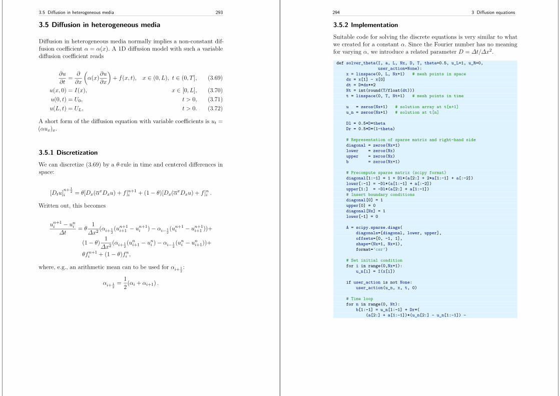
3.5 Diffusion in heterogeneous media 293
3.5 Diffusion in heterogeneous media
Diffusion in heterogeneous media normally implies a non-constant dif-fusion coefficient α = α(x). A 1D diffusion model with such a variablediffusion coefficient reads
∂u
∂t= ∂
∂x
(α(x)∂u
∂x
)+ f(x, t), x ∈ (0, L), t ∈ (0, T ], (3.69)
u(x, 0) = I(x), x ∈ [0, L], (3.70)u(0, t) = U0, t > 0, (3.71)u(L, t) = UL, t > 0. (3.72)
A short form of the diffusion equation with variable coefficients is ut =(αux)x.
3.5.1 Discretization
We can discretize (3.69) by a θ-rule in time and centered differences inspace:
[Dtu]n+ 12
i = θ[Dx(αxDxu) + f ]n+1i + (1− θ)[Dx(αxDxu) + f ]ni .
Written out, this becomes
un+1i − uni∆t
= θ1
∆x2 (αi+ 12(un+1i+1 − un+1
i )− αi− 12(un+1i − un+1
i+1 ))+
(1− θ) 1∆x2 (αi+ 1
2(uni+1 − uni )− αi− 1
2(uni − uni+1))+
θfn+1i + (1− θ)fni ,
where, e.g., an arithmetic mean can to be used for αi+ 12:
αi+ 12
= 12(αi + αi+1) .
294 3 Diffusion equations
3.5.2 Implementation
Suitable code for solving the discrete equations is very similar to whatwe created for a constant α. Since the Fourier number has no meaningfor varying α, we introduce a related parameter D = ∆t/∆x2.
def solver_theta(I, a, L, Nx, D, T, theta=0.5, u_L=1, u_R=0,user_action=None):
x = linspace(0, L, Nx+1) # mesh points in spacedx = x[1] - x[0]dt = D*dx**2Nt = int(round(T/float(dt)))t = linspace(0, T, Nt+1) # mesh points in time
u = zeros(Nx+1) # solution array at t[n+1]u_n = zeros(Nx+1) # solution at t[n]
Dl = 0.5*D*thetaDr = 0.5*D*(1-theta)
# Representation of sparse matrix and right-hand sidediagonal = zeros(Nx+1)lower = zeros(Nx)upper = zeros(Nx)b = zeros(Nx+1)
# Precompute sparse matrix (scipy format)diagonal[1:-1] = 1 + Dl*(a[2:] + 2*a[1:-1] + a[:-2])lower[:-1] = -Dl*(a[1:-1] + a[:-2])upper[1:] = -Dl*(a[2:] + a[1:-1])# Insert boundary conditionsdiagonal[0] = 1upper[0] = 0diagonal[Nx] = 1lower[-1] = 0
A = scipy.sparse.diags(diagonals=[diagonal, lower, upper],offsets=[0, -1, 1],shape=(Nx+1, Nx+1),format=’csr’)
# Set initial conditionfor i in range(0,Nx+1):
u_n[i] = I(x[i])
if user_action is not None:user_action(u_n, x, t, 0)
# Time loopfor n in range(0, Nt):
b[1:-1] = u_n[1:-1] + Dr*((a[2:] + a[1:-1])*(u_n[2:] - u_n[1:-1]) -
3.5 Diffusion in heterogeneous media 295
(a[1:-1] + a[0:-2])*(u_n[1:-1] - u_n[:-2]))# Boundary conditionsb[0] = u_L(t[n+1])b[-1] = u_R(t[n+1])# Solveu[:] = scipy.sparse.linalg.spsolve(A, b)
if user_action is not None:user_action(u, x, t, n+1)
# Switch variables before next stepu_n, u = u, u_n
The code is found in the file diffu1D_vc.py.
3.5.3 Stationary solution
As t → ∞, the solution of the problem (3.69)-(3.72) will approach astationary limit where ∂u/∂t = 0. The governing equation is then
d
dx
(αdu
dx
)= 0, (3.73)
with boundary conditions u(0) = U0 and u(L) = uL. It is possibleto obtain an exact solution of (3.73) for any α. Integrating twice andapplying the boundary conditions to determine the integration constantsgives
u(x) = U0 + (UL − U0)∫ x
0 (α(ξ))−1dξ∫ L
0 (α(ξ))−1dξ. (3.74)
3.5.4 Piecewise constant medium
Consider a medium built of M layers. The layer boundaries are denotedb0, . . . , bM , where b0 = 0 and bM = L. If the layers potentially havedifferent material properties, but these properties are constant withineach layer, we can express α as a piecewise constant function accordingto
296 3 Diffusion equations
α(x) =
α0, b0 ≤ x < b1,...αi, bi ≤ x < bi+1,...αM−1, bM−1 ≤ x ≤ bM .
(3.75)
The exact solution (3.74) in case of such a piecewise constant α functionis easy to derive. Assume that x is in the m-th layer: x ∈ [bm, bm+1].In the integral
∫ x0 (a(ξ))−1dξ we must integrate through the first m− 1
layers and then add the contribution from the remaining part x − bminto the m-th layer:
u(x) = U0+(UL−U0)∑m−1j=0 (bj+1 − bj)/α(bj) + (x− bm)/α(bm)
∑M−1j=0 (bj+1 − bj)/α(bj)
(3.76)
Remark. It may sound strange to have a discontinuous α in a differentialequation where one is to differentiate, but a discontinuous α is compen-sated by a discontinuous ux such that αux is continuous and thereforecan be differentiated as (αux)x.
3.5.5 Implementation of diffusion in a piecewise constantmedium
Programming with piecewise function definitions quickly becomes cum-bersome as the most naive approach is to test for which interval x lies,and then start evaluating a formula like (3.76). In Python, vectorizedexpressions may help to speed up the computations. The convenienceclasses PiecewiseConstant and IntegratedPiecewiseConstant in theHeaviside module were made to simplify programming with functionslike (3.5.4) and expressions like (3.76). These utilities not only representpiecewise constant functions, but also smoothed versions of them wherethe discontinuities can be smoothed out in a controlled fashion.
The PiecewiseConstant class is created by sending in the domain asa 2-tuple or 2-list and a data object describing the boundaries b0, . . . , bMand the corresponding function values α0, . . . , αM−1. More precisely, datais a nested list, where data[i][0] holds bi and data[i][1] holds thecorresponding value αi, for i = 0, . . . ,M − 1. Given bi and αi in arrays band a, it is easy to fill out the nested list data.
3.5 Diffusion in heterogeneous media 297
In our application, we want to represent α and 1/α as piecewiseconstant functions, in addition to the u(x) function which involves theintegrals of 1/α. A class creating the functions we need and a methodfor evaluating u, can take the form
class SerialLayers:"""b: coordinates of boundaries of layers, b[0] is left boundaryand b[-1] is right boundary of the domain [0,L].a: values of the functions in each layer (len(a) = len(b)-1).U_0: u(x) value at left boundary x=0=b[0].U_L: u(x) value at right boundary x=L=b[0]."""
def __init__(self, a, b, U_0, U_L, eps=0):self.a, self.b = np.asarray(a), np.asarray(b)self.eps = eps # smoothing parameter for smoothed aself.U_0, self.U_L = U_0, U_L
a_data = [[bi, ai] for bi, ai in zip(self.b, self.a)]domain = [b[0], b[-1]]self.a_func = PiecewiseConstant(domain, a_data, eps)
# inv_a = 1/a is needed in formulasinv_a_data = [[bi, 1./ai] for bi, ai in zip(self.b, self.a)]self.inv_a_func = \
PiecewiseConstant(domain, inv_a_data, eps)self.integral_of_inv_a_func = \
IntegratedPiecewiseConstant(domain, inv_a_data, eps)# Denominator in the exact formula is constantself.inv_a_0L = self.integral_of_inv_a_func(b[-1])
def __call__(self, x):solution = self.U_0 + (self.U_L-self.U_0)*\
self.integral_of_inv_a_func(x)/self.inv_a_0Lreturn solution
A visualization method is also convenient to have. Below we plot u(x)along with α(x) (which works well as long as maxα(x) is of the samesize as max u = max(U0, UL)).
class SerialLayers:...
def plot(self):x, y_a = self.a_func.plot()x = np.asarray(x); y_a = np.asarray(y_a)y_u = self.u_exact(x)import matplotlib.pyplot as pltplt.figure()plt.plot(x, y_u, ’b’)plt.hold(’on’) # Matlab style
298 3 Diffusion equations
plt.plot(x, y_a, ’r’)ymin = -0.1ymax = 1.2*max(y_u.max(), y_a.max())plt.axis([x[0], x[-1], ymin, ymax])plt.legend([’solution $u$’, ’coefficient $a$’], loc=’upper left’)if self.eps > 0:
plt.title(’Smoothing eps: %s’ % self.eps)plt.savefig(’tmp.pdf’)plt.savefig(’tmp.png’)plt.show()
Figure 3.12 shows the case where
b = [0, 0.25, 0.5, 1] # material boundariesa = [0.2, 0.4, 4] # material valuesU_0 = 0.5; U_L = 5 # boundary conditions
0.0 0.2 0.4 0.6 0.8 1.00
1
2
3
4
5
6solution ucoefficient a
Fig. 3.12 Solution of the stationary diffusion equation corresponding to a piecewiseconstant diffusion coefficient.
By adding the eps parameter to the constructor of the SerialLayersclass, we can experiment with smoothed versions of α and see the (small)impact on u. Figure 3.13 shows the result.
3.5 Diffusion in heterogeneous media 299
0.0 0.2 0.4 0.6 0.8 1.00
1
2
3
4
5
6 Smoothed discontinuous coefficient (eps=0.05)
solution ucoefficient a
Fig. 3.13 Solution of the stationary diffusion equation corresponding to a smoothedpiecewise constant diffusion coefficient.
3.5.6 Axi-symmetric diffusion
Suppose we have a diffusion process taking place in a straight tube withradius R. We assume axi-symmetry such that u is just a function ofr and t, r being the radial distance from the center axis of the tubeto a point. With such axi-symmetry it is advantageous to introducecylindrical coordinates r, θ, and z, where z is in the direction of the tubeand (r, θ) are polar coordinates in a cross section. Axi-symmetry meansthat all quantities are independent of θ. From the relations x = cos θ,y = sin θ, and z = z, between Cartesian and cylindrical coordinates,one can (with some effort) derive the diffusion equation in cylindricalcoordinates, which with axi-symmetry takes the form
∂u
∂t= 1r
∂
∂r
(rα(r, z)∂u
∂r
)+ ∂
∂z
(α(r, z)∂u
∂z
)+ f(r, z, t) .
Let us assume that u does not change along the tube axis so it sufficesto compute variations in a cross section. Then ∂u/∂z = 0 and the we
300 3 Diffusion equations
have a 1D diffusion equation in the radial coordinate r and time t. Inparticular, we shall address the initial-boundary value problem
∂u
∂t= 1r
∂
∂r
(rα(r)∂u
∂r
)+ f(t),r ∈ (0, R), t ∈ (0, T ], (3.77)
∂u
∂r(0, t) = 0, t ∈ (0, T ], (3.78)
u(R, t) = 0, t ∈ (0, T ], (3.79)u(r, 0) = I(r), r ∈ [0, R]. (3.80)
The condition (3.78) is a necessary symmetry condition at r = 0, while(3.79) could be any Dirichlet or Neumann condition (or Robin conditionin case of cooling or heating).
The finite difference approximation will need the discretized versionof the PDE for r = 0 (just as we use the PDE at the boundary whenimplementing Neumann conditions). However, discretizing the PDE atr = 0 poses a problem because of the 1/r factor. We therefore need towork out the PDE for discretization at r = 0 with care. Let us, for thecase of constant α, expand the spatial derivative term to
α∂2u
∂r2 + α1r
∂u
∂r.
The last term faces a difficulty at r = 0, since it becomes a 0/0 expressioncaused by the symmetry condition at r = 0. However, L’Hosptial’s rulecan be used:
limr→0
1r
∂u
∂r= ∂2u
∂r2 .
The PDE at r = 0 therefore becomes
∂u
∂t= 2α∂
2u
∂r2 + f(t) . (3.81)
For a variable coefficient α(r) the expanded spatial derivative term reads
α(r)∂2u
∂r2 + 1r
(α(r) + rα′(r))∂u∂r
.
We are interested in this expression for r = 0. A necessary conditionfor u to be axi-symmetric is that all input data, including α, must also
3.5 Diffusion in heterogeneous media 301
be axi-symmetric, implying that α′(0) = 0 (the second term vanishesanyway because of r = 0). The limit of interest is
limr→0
1rα(r)∂u
∂r= α(0)∂
2u
∂r2 .
The PDE at r = 0 now looks like
∂u
∂t= 2α(0)∂
2u
∂r2 + f(t), (3.82)
so there is no essential difference between the constant coefficient andvariable coefficient cases.
The second-order derivative in (3.81) and (3.82) is discretized in theusual way.
2α ∂2
∂r2u(r0, tn) ≈ [2α2DrDru]n0 = 2αun1 − 2un0 + un−1
∆r2 .
The fictitious value un−1 can be eliminated using the discrete symmetrycondition
[D2ru = 0]n0 ⇒ un−1 = un1 ,
which then gives the modified approximation to the term with the second-order derivative of u in r at r = 0:
4αun1 − un0∆r2 . (3.83)
The discretization of the term with the second-order derivative in r atany internal mesh point is straightforward:
[1r
∂
∂r
(rα∂u
∂r
)]n
i
≈ [r−1Dr(rαDru)]ni
= 1ri
1∆r2
(ri+ 1
2αi+ 1
2(uni+1 − uni )− ri− 1
2αi− 1
2(uni − uni−1)
).
To complete the discretization, we need a scheme in time, but thatcan be done as before and does not interfere with the discretization inspace.
302 3 Diffusion equations
3.5.7 Spherically-symmetric diffusion
Discretization in spherical coordinates. Let us now pose the problemfrom Section 3.5.6 in spherical coordinates, where u only depends on theradial coordinate r and time t. That is, we have spherical symmetry. Forsimplicity we restrict the diffusion coefficient α to be a constant. ThePDE reads
∂u
∂t= α
rγ∂
∂r
(rγ∂u
∂r
)+ f(t), (3.84)
for r ∈ (0, R) and t ∈ (0, T ]. The parameter γ is 2 for spherically-symmetric problems and 1 for axi-symmetric problems. The boundaryand initial conditions have the same mathematical form as in (3.77)-(3.80).
Since the PDE in spherical coordinates has the same form as the PDEin Section 3.5.6, just with the γ parameter being different, we can usethe same discretization approach. At the origin r = 0 we get problemswith the term
γ
r
∂u
∂t,
but L’Hosptial’s rule shows that this term equals γ∂2u/∂r2, and thePDE at r = 0 becomes
∂u
∂t= (γ + 1)α∂
2u
∂r2 + f(t) . (3.85)
The associated discrete form is then
[Dtu = 12(γ + 1)α([DrDru
t + ft]ni , (3.86)
for a Crank-Nicolson scheme.
Discretization in Cartesian coordinates. The spherically-symmetricspatial derivative can be transformed to the Cartesian counterpart byintroducing
v(r, t) = ru(r, t) .
Inserting u = v/r in
1r2
∂
∂r
(α(r)r2∂u
∂r
),
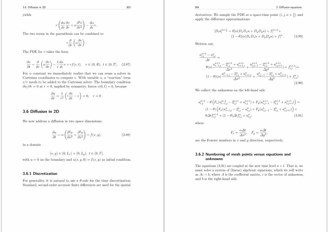
3.6 Diffusion in 2D 303
yields
r
(dα
dr
∂v
∂r+ α
∂2v
∂r2
)− dα
drv .
The two terms in the parenthesis can be combined to
r∂
∂r
(α∂v
∂r
).
The PDE for v takes the form
∂v
∂t= ∂
∂r
(α∂v
∂r
)− 1r
dα
drv + rf(r, t), r ∈ (0, R), t ∈ (0, T ] . (3.87)
For α constant we immediately realize that we can reuse a solver inCartesian coordinates to compute v. With variable α, a “reaction” termv/r needs to be added to the Cartesian solver. The boundary condition∂u/∂r = 0 at r = 0, implied by symmetry, forces v(0, t) = 0, because
∂u
∂r= 1r2
(r∂v
∂r− v
)= 0, r = 0 .
3.6 Diffusion in 2D
We now address a diffusion in two space dimensions:
∂u
∂t= α
(∂2u
∂x2 + ∂2u
∂x2
)+ f(x, y), (3.88)
in a domain
(x, y) ∈ (0, Lx)× (0, Ly), t ∈ (0, T ],
with u = 0 on the boundary and u(x, y, 0) = I(x, y) as initial condition.
3.6.1 Discretization
For generality, it is natural to use a θ-rule for the time discretization.Standard, second-order accurate finite differences are used for the spatial
304 3 Diffusion equations
derivatives. We sample the PDE at a space-time point (i, j, n+ 12) and
apply the difference approximations:
[Dtu]n+ 12 = θ[α(DxDxu+DyDyu) + f ]n+1+
(1− θ)[α(DxDxu+DyDyu) + f ]n . (3.89)
Written out,
un+1i,j − uni,j∆t
=
θ(α(un+1i−1,j − 2n+1
i,j + un+1i+1,j
∆x2 +un+1i,j−1 − 2n+1
i,j + un+1i,j+1
∆y2 ) + fn+1i,j )+
(1− θ)(α(uni−1,j − 2ni,j + uni+1,j
∆x2 +uni,j−1 − 2ni,j + uni,j+1
∆y2 ) + fni,j)
(3.90)
We collect the unknowns on the left-hand side
un+1i,j − θ
(Fx(un+1
i−1,j − 2n+1i,j + un+1
i,j ) + Fy(un+1i,j−1 − 2n+1
i,j + un+1i,j+1)
)=
(1− θ)(Fx(uni−1,j − 2ni,j + uni,j) + Fy(uni,j−1 − 2ni,j + uni,j+1)
)+
θ∆tfn+1i,j + (1− θ)∆tfni,j + uni,j , (3.91)
where
Fx = α∆t
∆x2 , Fy = α∆t
∆y2 ,
are the Fourier numbers in x and y direction, respectively.
3.6.2 Numbering of mesh points versus equations andunknowns
The equations (3.91) are coupled at the new time level n+ 1. That is, wemust solve a system of (linear) algebraic equations, which we will writeas Ac = b, where A is the coefficient matrix, c is the vector of unknowns,and b is the right-hand side.
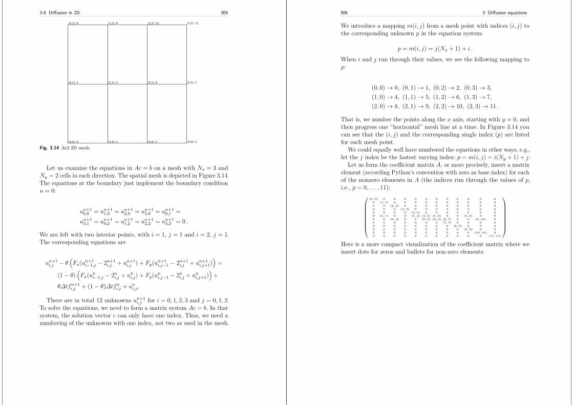
3.6 Diffusion in 2D 305
(0,2): 8
(0,1): 4
(0,0): 0 (3,0): 3
(3,1): 7
(1,2): 9
(1,0): 1
(1,1): 5
(3,2): 11
(2,1): 6
(2,0): 2
(2,2): 10
Fig. 3.14 3x2 2D mesh.
Let us examine the equations in Ac = b on a mesh with Nx = 3 andNy = 2 cells in each direction. The spatial mesh is depicted in Figure 3.14.The equations at the boundary just implement the boundary conditionu = 0:
un+10,0 = un+1
1,0 = un+12,0 = un+1
3,0 = un+10,1 =
un+13,1 = un+1
0,2 = un+11,2 = un+1
2,2 = un+13,2 = 0 .
We are left with two interior points, with i = 1, j = 1 and i = 2, j = 1.The corresponding equations are
un+1i,j − θ
(Fx(un+1
i−1,j − 2n+1i,j + un+1
i,j ) + Fy(un+1i,j−1 − 2n+1
i,j + un+1i,j+1)
)=
(1− θ)(Fx(uni−1,j − 2ni,j + uni,j) + Fy(uni,j−1 − 2ni,j + uni,j+1)
)+
θ∆tfn+1i,j + (1− θ)∆tfni,j + uni,j ,
There are in total 12 unknowns un+1i,j for i = 0, 1, 2, 3 and j = 0, 1, 2.
To solve the equations, we need to form a matrix system Ac = b. In thatsystem, the solution vector c can only have one index. Thus, we need anumbering of the unknowns with one index, not two as used in the mesh.
306 3 Diffusion equations
We introduce a mapping m(i, j) from a mesh point with indices (i, j) tothe corresponding unknown p in the equation system:
p = m(i, j) = j(Nx + 1) + i .
When i and j run through their values, we see the following mapping top:
(0, 0)→ 0, (0, 1)→ 1, (0, 2)→ 2, (0, 3)→ 3,(1, 0)→ 4, (1, 1)→ 5, (1, 2)→ 6, (1, 3)→ 7,(2, 0)→ 8, (2, 1)→ 9, (2, 2)→ 10, (2, 3)→ 11 .
That is, we number the points along the x axis, starting with y = 0, andthen progress one “horizontal” mesh line at a time. In Figure 3.14 youcan see that the (i, j) and the corresponding single index (p) are listedfor each mesh point.
We could equally well have numbered the equations in other ways, e.g.,let the j index be the fastest varying index: p = m(i, j) = i(Ny + 1) + j.
Let us form the coefficient matrix A, or more precisely, insert a matrixelement (according Python’s convention with zero as base index) for eachof the nonzero elements in A (the indices run through the values of p,i.e., p = 0, . . . , 11):
(0, 0) 0 0 0 0 0 0 0 0 0 0 00 (1, 1) 0 0 0 0 0 0 0 0 0 00 0 (2, 2) 0 0 0 0 0 0 0 0 00 0 0 (3, 3) 0 0 0 0 0 0 0 00 0 0 0 (4, 4) 0 0 0 0 0 0 00 (5, 1) 0 0 (5, 4) (5, 5) (5, 6) 0 0 (5, 9) 0 00 0 (6, 2) 0 0 (6, 5) (6, 6) (6, 7) 0 0 (6, 10) 00 0 0 0 0 0 0 (7, 7) 0 0 0 00 0 0 0 0 0 0 0 (8, 8) 0 0 00 0 0 0 0 0 0 0 0 (9, 9) 0 00 0 0 0 0 0 0 0 0 0 (10, 10) 00 0 0 0 0 0 0 0 0 0 0 (11, 11)
Here is a more compact visualization of the coefficient matrix where weinsert dots for zeros and bullets for non-zero elements:
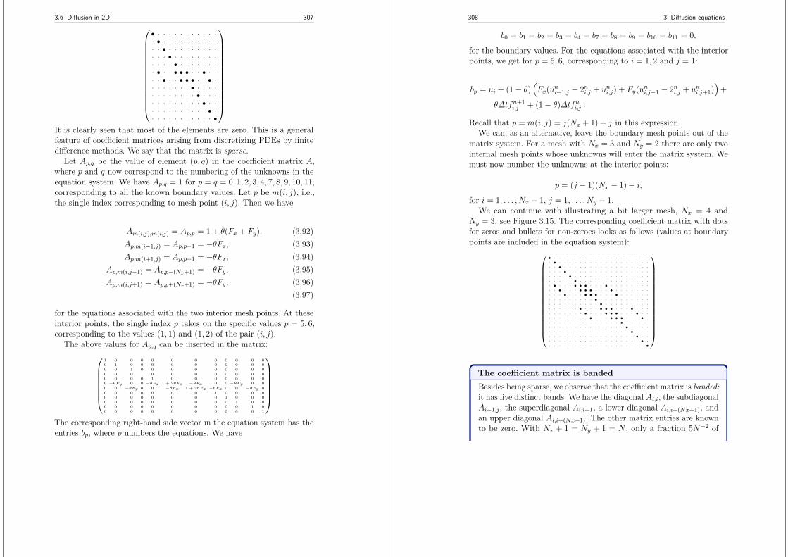
3.6 Diffusion in 2D 307
• · · · · · · · · · · ·· • · · · · · · · · · ·· · • · · · · · · · · ·· · · • · · · · · · · ·· · · · • · · · · · · ·· • · · • • • · · • · ·· · • · · • • • · · • ·· · · · · · · • · · · ·· · · · · · · · • · · ·· · · · · · · · · • · ·· · · · · · · · · · • ·· · · · · · · · · · · •
It is clearly seen that most of the elements are zero. This is a generalfeature of coefficient matrices arising from discretizing PDEs by finitedifference methods. We say that the matrix is sparse.
Let Ap,q be the value of element (p, q) in the coefficient matrix A,where p and q now correspond to the numbering of the unknowns in theequation system. We have Ap,q = 1 for p = q = 0, 1, 2, 3, 4, 7, 8, 9, 10, 11,corresponding to all the known boundary values. Let p be m(i, j), i.e.,the single index corresponding to mesh point (i, j). Then we have
Am(i,j),m(i,j) = Ap,p = 1 + θ(Fx + Fy), (3.92)Ap,m(i−1,j) = Ap,p−1 = −θFx, (3.93)Ap,m(i+1,j) = Ap,p+1 = −θFx, (3.94)
Ap,m(i,j−1) = Ap,p−(Nx+1) = −θFy, (3.95)Ap,m(i,j+1) = Ap,p+(Nx+1) = −θFy, (3.96)
(3.97)
for the equations associated with the two interior mesh points. At theseinterior points, the single index p takes on the specific values p = 5, 6,corresponding to the values (1, 1) and (1, 2) of the pair (i, j).
The above values for Ap,q can be inserted in the matrix:
1 0 0 0 0 0 0 0 0 0 0 00 1 0 0 0 0 0 0 0 0 0 00 0 1 0 0 0 0 0 0 0 0 00 0 0 1 0 0 0 0 0 0 0 00 0 0 0 1 0 0 0 0 0 0 00 −θFy 0 0 −θFx 1 + 2θFx −θFx 0 0 −θFy 0 00 0 −θFy 0 0 −θFx 1 + 2θFx −θFx 0 0 −θFy 00 0 0 0 0 0 0 1 0 0 0 00 0 0 0 0 0 0 0 1 0 0 00 0 0 0 0 0 0 0 0 1 0 00 0 0 0 0 0 0 0 0 0 1 00 0 0 0 0 0 0 0 0 0 0 1
The corresponding right-hand side vector in the equation system has theentries bp, where p numbers the equations. We have
308 3 Diffusion equations
b0 = b1 = b2 = b3 = b4 = b7 = b8 = b9 = b10 = b11 = 0,
for the boundary values. For the equations associated with the interiorpoints, we get for p = 5, 6, corresponding to i = 1, 2 and j = 1:
bp = ui + (1− θ)(Fx(uni−1,j − 2ni,j + uni,j) + Fy(uni,j−1 − 2ni,j + uni,j+1)
)+
θ∆tfn+1i,j + (1− θ)∆tfni,j .
Recall that p = m(i, j) = j(Nx + 1) + j in this expression.We can, as an alternative, leave the boundary mesh points out of the
matrix system. For a mesh with Nx = 3 and Ny = 2 there are only twointernal mesh points whose unknowns will enter the matrix system. Wemust now number the unknowns at the interior points:
p = (j − 1)(Nx − 1) + i,
for i = 1, . . . , Nx − 1, j = 1, . . . , Ny − 1.We can continue with illustrating a bit larger mesh, Nx = 4 and
Ny = 3, see Figure 3.15. The corresponding coefficient matrix with dotsfor zeros and bullets for non-zeroes looks as follows (values at boundarypoints are included in the equation system):
• · · · · · · · · · · · · · · · · · · ·· • · · · · · · · · · · · · · · · · · ·· · • · · · · · · · · · · · · · · · · ·· · · • · · · · · · · · · · · · · · · ·· · · · • · · · · · · · · · · · · · · ·· · · · · • · · · · · · · · · · · · · ·· • · · · • • • · · · • · · · · · · · ·· · • · · · • • • · · · • · · · · · · ·· · · • · · · • • • · · · • · · · · · ·· · · · · · · · · • · · · · · · · · · ·· · · · · · · · · · • · · · · · · · · ·· · · · · · • · · · • • • · · · • · · ·· · · · · · · • · · · • • • · · · • · ·· · · · · · · · • · · · • • • · · · • ·· · · · · · · · · · · · · · • · · · · ·· · · · · · · · · · · · · · · • · · · ·· · · · · · · · · · · · · · · · • · · ·· · · · · · · · · · · · · · · · · • · ·· · · · · · · · · · · · · · · · · · • ·· · · · · · · · · · · · · · · · · · · •
The coefficient matrix is bandedBesides being sparse, we observe that the coefficient matrix is banded:it has five distinct bands. We have the diagonal Ai,i, the subdiagonalAi−1,j , the superdiagonal Ai,i+1, a lower diagonal Ai,i−(Nx+1), andan upper diagonal Ai,i+(Nx+1). The other matrix entries are knownto be zero. With Nx + 1 = Ny + 1 = N , only a fraction 5N−2 of
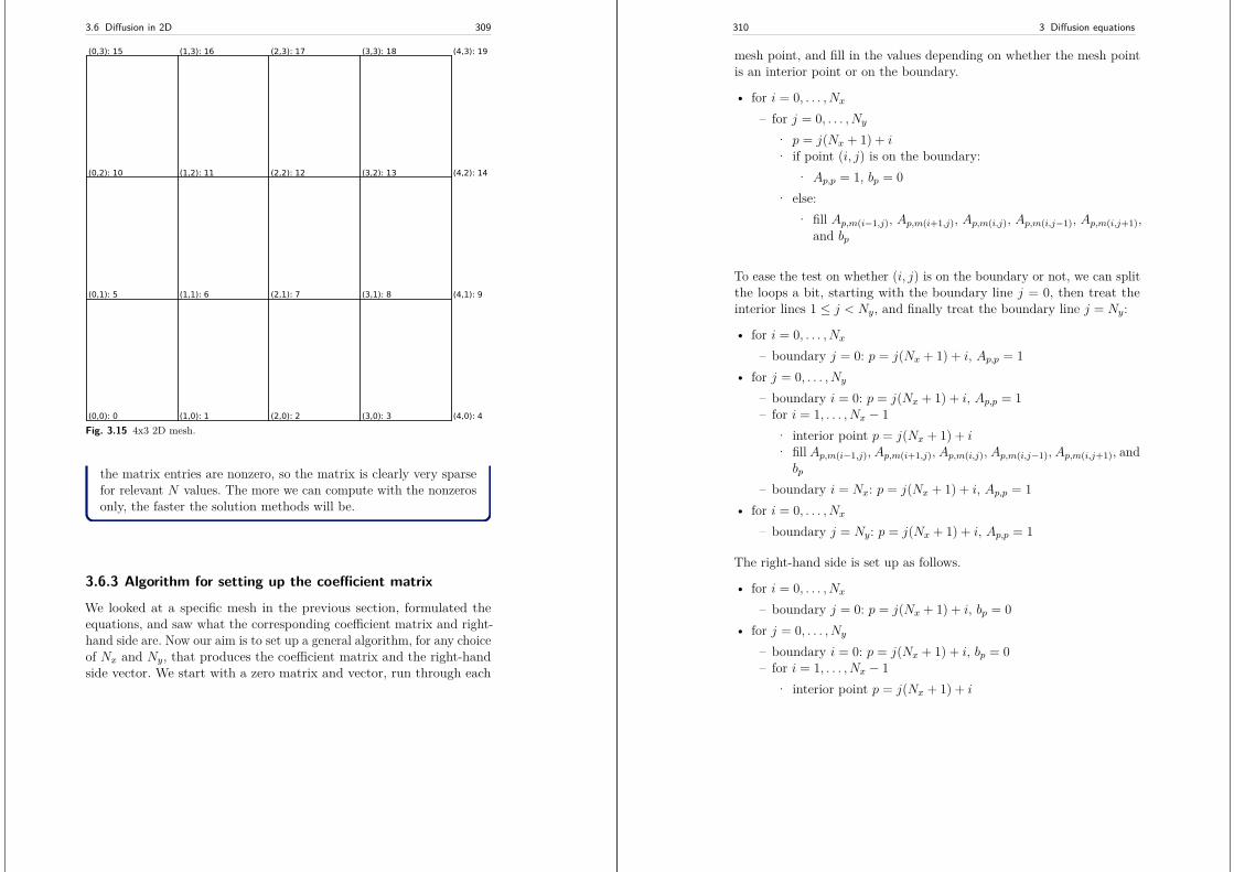
3.6 Diffusion in 2D 309
(0,2): 10
(0,1): 5
(0,0): 0 (3,0): 3
(3,1): 8
(1,2): 11
(1,0): 1
(1,1): 6
(3,2): 13
(1,3): 16 (4,3): 19
(4,2): 14
(3,3): 18
(2,1): 7
(2,0): 2
(4,1): 9
(4,0): 4
(2,3): 17
(2,2): 12
(0,3): 15
Fig. 3.15 4x3 2D mesh.
the matrix entries are nonzero, so the matrix is clearly very sparsefor relevant N values. The more we can compute with the nonzerosonly, the faster the solution methods will be.
3.6.3 Algorithm for setting up the coefficient matrix
We looked at a specific mesh in the previous section, formulated theequations, and saw what the corresponding coefficient matrix and right-hand side are. Now our aim is to set up a general algorithm, for any choiceof Nx and Ny, that produces the coefficient matrix and the right-handside vector. We start with a zero matrix and vector, run through each
310 3 Diffusion equations
mesh point, and fill in the values depending on whether the mesh pointis an interior point or on the boundary.
• for i = 0, . . . , Nx
– for j = 0, . . . , Ny
· p = j(Nx + 1) + i· if point (i, j) is on the boundary:
· Ap,p = 1, bp = 0· else:
· fill Ap,m(i−1,j), Ap,m(i+1,j), Ap,m(i,j), Ap,m(i,j−1), Ap,m(i,j+1),and bp
To ease the test on whether (i, j) is on the boundary or not, we can splitthe loops a bit, starting with the boundary line j = 0, then treat theinterior lines 1 ≤ j < Ny, and finally treat the boundary line j = Ny:
• for i = 0, . . . , Nx
– boundary j = 0: p = j(Nx + 1) + i, Ap,p = 1• for j = 0, . . . , Ny
– boundary i = 0: p = j(Nx + 1) + i, Ap,p = 1– for i = 1, . . . , Nx − 1
· interior point p = j(Nx + 1) + i· fill Ap,m(i−1,j), Ap,m(i+1,j), Ap,m(i,j), Ap,m(i,j−1), Ap,m(i,j+1), andbp
– boundary i = Nx: p = j(Nx + 1) + i, Ap,p = 1• for i = 0, . . . , Nx
– boundary j = Ny: p = j(Nx + 1) + i, Ap,p = 1
The right-hand side is set up as follows.
• for i = 0, . . . , Nx
– boundary j = 0: p = j(Nx + 1) + i, bp = 0• for j = 0, . . . , Ny
– boundary i = 0: p = j(Nx + 1) + i, bp = 0– for i = 1, . . . , Nx − 1
· interior point p = j(Nx + 1) + i
3.6 Diffusion in 2D 311
· fill bp– boundary i = Nx: p = j(Nx + 1) + i, bp = 0
• for i = 0, . . . , Nx
– boundary j = Ny: p = j(Nx + 1) + i, bp = 0
3.6.4 Implementation with a dense coefficient matrix
The goal now is to map the algorithms in the previous section to Pythoncode. One should, for computational efficiency reasons, take advantageof the fact that the coefficient matrix is sparse and/or banded, i.e., takeadvantage of all the zeros. However, we first demonstrate how to fill anN ×N dense square matrix, where N is the number of unknowns, hereN = (Nx + 1)(Ny + 1). The dense matrix is much easier to understandthan the sparse matrix case.
import numpy as np
def solver_dense(I, a, f, Lx, Ly, Nx, Ny, dt, T, theta=0.5, user_action=None):"""Solve u_t = a*(u_xx + u_yy) + f, u(x,y,0)=I(x,y), with u=0on the boundary, on [0,Lx]x[0,Ly]x[0,T], with time step dt,using the theta-scheme."""x = np.linspace(0, Lx, Nx+1) # mesh points in x diry = np.linspace(0, Ly, Ny+1) # mesh points in y dirdx = x[1] - x[0]dy = y[1] - y[0]
dt = float(dt) # avoid integer divisionNt = int(round(T/float(dt)))t = np.linspace(0, Nt*dt, Nt+1) # mesh points in time
# Mesh Fourier numbers in each directionFx = a*dt/dx**2Fy = a*dt/dy**2
The un+1i,j and uni,j mesh functions are represented by their spatial values
at the mesh points:
u = np.zeros((Nx+1, Ny+1)) # unknown u at new time levelu_n = np.zeros((Nx+1, Ny+1)) # u at the previous time level
It is a good habit (for extensions) to introduce index sets for all meshpoints:
312 3 Diffusion equations
Ix = range(0, Nx+1)Iy = range(0, Ny+1)It = range(0, Nt+1)
The initial condition is easy to fill in:
# Load initial condition into u_nfor i in Ix:
for j in Iy:u_n[i,j] = I(x[i], y[j])
The memory for the coefficient matrix and right-hand side vector isallocated by
N = (Nx+1)*(Ny+1) # no of unknownsA = np.zeros((N, N))b = np.zeros(N)
The filling of A goes like this:
m = lambda i, j: j*(Nx+1) + i
# Equations corresponding to j=0, i=0,1,... (u known)j = 0for i in Ix:
p = m(i,j); A[p, p] = 1
# Loop over all internal mesh points in y diretion# and all mesh points in x directionfor j in Iy[1:-1]:
i = 0; p = m(i,j); A[p, p] = 1 # Boundaryfor i in Ix[1:-1]: # Interior points
p = m(i,j)A[p, m(i,j-1)] = - theta*FyA[p, m(i-1,j)] = - theta*FxA[p, p] = 1 + 2*theta*(Fx+Fy)A[p, m(i+1,j)] = - theta*FxA[p, m(i,j+1)] = - theta*Fy
i = Nx; p = m(i,j); A[p, p] = 1 # Boundary# Equations corresponding to j=Ny, i=0,1,... (u known)j = Nyfor i in Ix:
p = m(i,j); A[p, p] = 1
Since A is independent of time, it can be filled once and for all before thetime loop. The right-hand side vector must be filled at each time levelinside the time loop:
import scipy.linalg
for n in It[0:-1]:# Compute bj = 0
3.6 Diffusion in 2D 313
for i in Ix:p = m(i,j); b[p] = 0 # Boundary
for j in Iy[1:-1]:i = 0; p = m(i,j); b[p] = 0 # Boundaryfor i in Ix[1:-1]: # Interior points
p = m(i,j)b[p] = u_n[i,j] + \
(1-theta)*(Fx*(u_n[i+1,j] - 2*u_n[i,j] + u_n[i-1,j]) +\Fy*(u_n[i,j+1] - 2*u_n[i,j] + u_n[i,j-1]))\
+ theta*dt*f(i*dx,j*dy,(n+1)*dt) + \(1-theta)*dt*f(i*dx,j*dy,n*dt)
i = Nx; p = m(i,j); b[p] = 0 # Boundaryj = Nyfor i in Ix:
p = m(i,j); b[p] = 0 # Boundary
# Solve matrix system A*c = bc = scipy.linalg.solve(A, b)
# Fill u with vector cfor i in Ix:
for j in Iy:u[i,j] = c[m(i,j)]
# Update u_n before next stepu_n, u = u, u_n
We use solve from scipy.linalg and not from numpy.linalg. Thedifference is stated below.
scipy.linalg versus numpy.linalg
Quote from the SciPy documentationa:scipy.linalg contains all the functions in numpy.linalg plus
some other more advanced ones not contained in numpy.linalg.Another advantage of using scipy.linalg over numpy.linalg is
that it is always compiled with BLAS/LAPACK support, whilefor NumPy this is optional. Therefore, the SciPy version might befaster depending on how NumPy was installed.
Therefore, unless you don’t want to add SciPy as a depen-dency to your NumPy program, use scipy.linalg instead ofnumpy.linalg.
a http://docs.scipy.org/doc/scipy/reference/tutorial/linalg.html
314 3 Diffusion equations
The code shown above is available in the solver_dense function inthe file diffu2D_u0.py, differing only in the boundary conditions, whichin the code can be an arbitrary function along each side of the domain.
We do not bother to look at vectorized versions of filling A sincea dense matrix is just used of pedagogical reasons for the very firstimplementation. Vectorization will be treated when A has a sparse matrixrepresentation, as in Section 3.6.7.
How to debug the computation of A and b
A good starting point for debugging the filling of A and b is tochoose a very coarse mesh, say Nx = Ny = 2, where there is justone internal mesh point, compute the equations by hand, and printout A and b for comparison in the code. If wrong elements in A or boccur, print out each assignment to elements in A and b inside theloops and compare with what you expect.
To let the user store, analyze, or visualize the solution at each timelevel, we include a callback function, named user_action, to be calledbefore the time loop and in each pass in that loop. The function has thesignature
user_action(u, x, xv, y, yv, t, n)
where u is a two-dimensional array holding the solution at time level nand time t[n]. The x and y coordinates of the mesh points are given bythe arrays x and y, respectively. The arrays xv and yv are vectorized rep-resentations of the mesh points such that vectorized function evaluationscan be invoked. The xv and yv arrays are defined by
xv = x[:,np.newaxis]yv = y[np.newaxis,:]
One can then evaluate, e.g., f(x, y, t) at all internal mesh points at timelevel n by first evaluating f at all points,
f_a = f(xv, yv, t[n])
and then use slices to extract a view of the values at the internal meshpoints: f_a[1:-1,1:-1]. The next section features an example on writinga user_action callback function.
3.6 Diffusion in 2D 315
3.6.5 Verification: exact numerical solution
A good test example to start with is one that preserves the solutionu = 0, i.e., f = 0 and I(x, y) = 0. This trivial solution can uncover somebugs.
The first real test example is based on having an exact solution of thediscrete equations. This solution is linear in time and quadratic in space:
u(x, y, t) = 5tx(Lx − x)y(y − Ly) .Inserting this manufactured solution in the PDE shows that the sourceterm f must be
f(x, y, t) = 5x(Lx − x)y(y − Ly) + 10αt(x(Lx − x) + y(y − Ly)) .
We can use the user_action function to compare the numericalsolution with the exact solution at each time level. A suitable helperfunction for checking the solution goes like this:
def quadratic(theta, Nx, Ny):
def u_exact(x, y, t):return 5*t*x*(Lx-x)*y*(Ly-y)
def I(x, y):return u_exact(x, y, 0)
def f(x, y, t):return 5*x*(Lx-x)*y*(Ly-y) + 10*a*t*(y*(Ly-y)+x*(Lx-x))
# Use rectangle to detect errors in switching i and j in schemeLx = 0.75Ly = 1.5a = 3.5dt = 0.5T = 2
def assert_no_error(u, x, xv, y, yv, t, n):"""Assert zero error at all mesh points."""u_e = u_exact(xv, yv, t[n])diff = abs(u - u_e).max()tol = 1E-12msg = ’diff=%g, step %d, time=%g’ % (diff, n, t[n])print msgassert diff < tol, msg
solver_dense(I, a, f, Lx, Ly, Nx, Ny,dt, T, theta, user_action=assert_no_error)
316 3 Diffusion equations
A true test function for checking the quadratic solution for severaldifferent meshes and θ values can take the form
def test_quadratic():# For each of the three schemes (theta = 1, 0.5, 0), a series of# meshes are tested (Nx > Ny and Nx < Ny)for theta in [1, 0.5, 0]:
for Nx in range(2, 6, 2):for Ny in range(2, 6, 2):
print ’testing for %dx%d mesh’ % (Nx, Ny)quadratic(theta, Nx, Ny)
3.6.6 Verification: convergence ratesFor 2D verification with convergence rate computations, the expressionsand computations just build naturally on what we saw for 1D diffusion.Truncation error analysis and other forms of error analysis point to anumerical error formula like
E = Ct∆tp + Cx∆x
2 + Cy∆y2,
where p, Ct, Cx, and Cy are constants. Often, the analysis of a Crank-Nicolson method can show that p = 2, while the Forward and BackwardEuler schemes have p = 1.
When checking the error formula empirically, we need to reduce it toa form E = Chr with a single discretization parameter h and some rater to be estimated. For the Backward Euler method, where p = 1, we canintroduce a single discretization parameter according to
h = ∆x2 = ∆y2, h = K−1∆t,
where K is a constant. The error formula then becomes
E = CtKh+ Cxh+ Cy = Ch, C = CtK + Cx + Cy .
The simplest choice is obviously K = 1. With the Forward Euler method,however, stability requires ∆t = hK ≤ h/(4α), so K ≤ 1/(4α).
For the Crank-Nicolson method, p = 2, and we can simply choose
h = ∆x = ∆y = ∆t,
since there is no restriction on ∆t in terms of ∆x and ∆y.A frequently used error measure is the `2 norm of the error mesh point
values. Section 2.2.3 and the formula (2.26) shows the error measure for
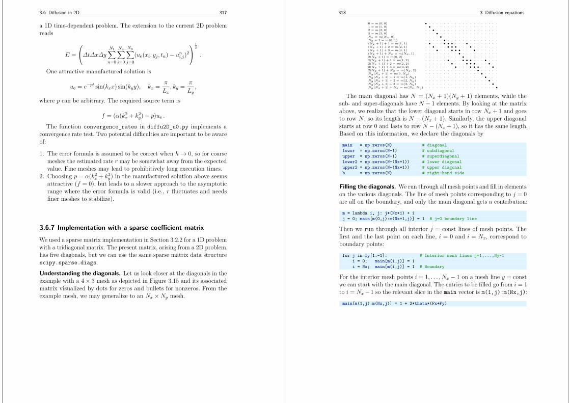
3.6 Diffusion in 2D 317
a 1D time-dependent problem. The extension to the current 2D problemreads
E =
∆t∆x∆y
Nt∑
n=0
Nx∑
i=0
Ny∑
j=0(ue(xi, yj , tn)− uni,j)2
12
.
One attractive manufactured solution is
ue = e−pt sin(kxx) sin(kyy), kx = π
Lx, ky = π
Ly,
where p can be arbitrary. The required source term is
f = (α(k2x + k2
y)− p)ue .The function convergence_rates in diffu2D_u0.py implements a
convergence rate test. Two potential difficulties are important to be awareof:
1. The error formula is assumed to be correct when h→ 0, so for coarsemeshes the estimated rate r may be somewhat away from the expectedvalue. Fine meshes may lead to prohibitively long execution times.
2. Choosing p = α(k2x + k2
y) in the manufactured solution above seemsattractive (f = 0), but leads to a slower approach to the asymptoticrange where the error formula is valid (i.e., r fluctuates and needsfiner meshes to stabilize).
3.6.7 Implementation with a sparse coefficient matrix
We used a sparse matrix implementation in Section 3.2.2 for a 1D problemwith a tridiagonal matrix. The present matrix, arising from a 2D problem,has five diagonals, but we can use the same sparse matrix data structurescipy.sparse.diags.
Understanding the diagonals. Let us look closer at the diagonals in theexample with a 4× 3 mesh as depicted in Figure 3.15 and its associatedmatrix visualized by dots for zeros and bullets for nonzeros. From theexample mesh, we may generalize to an Nx ×Ny mesh.
318 3 Diffusion equations
0 = m(0, 0) • · · · · · · · · · · · · · · · · · · ·1 = m(1, 0) · • · · · · · · · · · · · · · · · · · ·2 = m(2, 0) · · • · · · · · · · · · · · · · · · · ·3 = m(3, 0) · · · • · · · · · · · · · · · · · · · ·Nx = m(Nx, 0) · · · · • · · · · · · · · · · · · · · ·Nx + 1 = m(0, 1) · · · · · • · · · · · · · · · · · · · ·(Nx + 1) + 1 = m(1, 1) · • · · · • • • · · · • · · · · · · · ·(Nx + 1) + 2 = m(2, 1) · · • · · · • • • · · · • · · · · · · ·(Nx + 1) + 3 = m(3, 1) · · · • · · · • • • · · · • · · · · · ·(Nx + 1) + Nx = m(Nx, 1) · · · · · · · · · • · · · · · · · · · ·2(Nx + 1) = m(0, 2) · · · · · · · · · · • · · · · · · · · ·2(Nx + 1) + 1 = m(1, 2) · · · · · · • · · · • • • · · · • · · ·2(Nx + 1) + 2 = m(2, 2) · · · · · · · • · · · • • • · · · • · ·2(Nx + 1) + 3 = m(3, 2) · · · · · · · · • · · · • • • · · · • ·2(Nx + 1) + Nx = m(Nx, 2) · · · · · · · · · · · · · · • · · · · ·Ny(Nx + 1) = m(0, Ny) · · · · · · · · · · · · · · · • · · · ·Ny(Nx + 1) + 1 = m(1, Ny) · · · · · · · · · · · · · · · · • · · ·Ny(Nx + 1) + 2 = m(2, Ny) · · · · · · · · · · · · · · · · · • · ·Ny(Nx + 1) + 3 = m(3, Ny) · · · · · · · · · · · · · · · · · · • ·Ny(Nx + 1) + Nx = m(Nx,Ny) · · · · · · · · · · · · · · · · · · · •
The main diagonal has N = (Nx + 1)(Ny + 1) elements, while thesub- and super-diagonals have N − 1 elements. By looking at the matrixabove, we realize that the lower diagonal starts in row Nx + 1 and goesto row N , so its length is N − (Nx + 1). Similarly, the upper diagonalstarts at row 0 and lasts to row N − (Nx + 1), so it has the same length.Based on this information, we declare the diagonals by
main = np.zeros(N) # diagonallower = np.zeros(N-1) # subdiagonalupper = np.zeros(N-1) # superdiagonallower2 = np.zeros(N-(Nx+1)) # lower diagonalupper2 = np.zeros(N-(Nx+1)) # upper diagonalb = np.zeros(N) # right-hand side
Filling the diagonals. We run through all mesh points and fill in elementson the various diagonals. The line of mesh points corresponding to j = 0are all on the boundary, and only the main diagonal gets a contribution:
m = lambda i, j: j*(Nx+1) + ij = 0; main[m(0,j):m(Nx+1,j)] = 1 # j=0 boundary line
Then we run through all interior j = const lines of mesh points. Thefirst and the last point on each line, i = 0 and i = Nx, correspond toboundary points:
for j in Iy[1:-1]: # Interior mesh lines j=1,...,Ny-1i = 0; main[m(i,j)] = 1i = Nx; main[m(i,j)] = 1 # Boundary
For the interior mesh points i = 1, . . . , Nx − 1 on a mesh line y = constwe can start with the main diagonal. The entries to be filled go from i = 1to i = Nx− 1 so the relevant slice in the main vector is m(1,j):m(Nx,j):
main[m(1,j):m(Nx,j)] = 1 + 2*theta*(Fx+Fy)
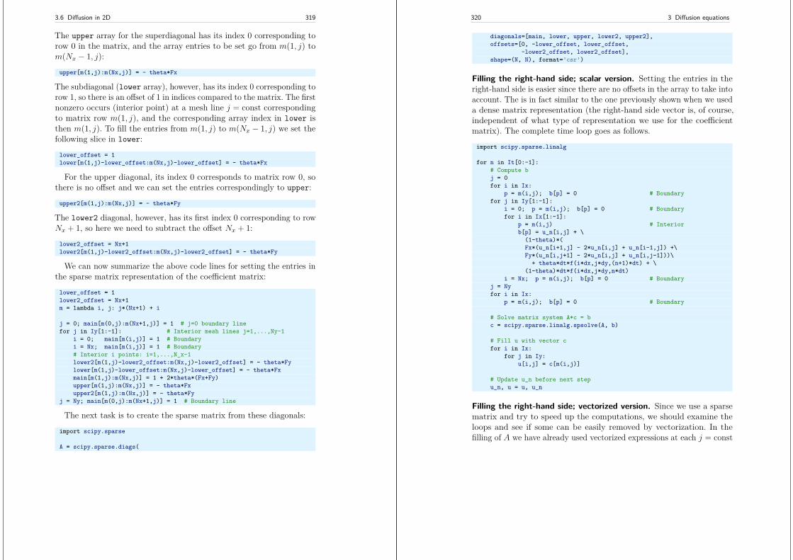
3.6 Diffusion in 2D 319
The upper array for the superdiagonal has its index 0 corresponding torow 0 in the matrix, and the array entries to be set go from m(1, j) tom(Nx − 1, j):
upper[m(1,j):m(Nx,j)] = - theta*Fx
The subdiagonal (lower array), however, has its index 0 corresponding torow 1, so there is an offset of 1 in indices compared to the matrix. The firstnonzero occurs (interior point) at a mesh line j = const correspondingto matrix row m(1, j), and the corresponding array index in lower isthen m(1, j). To fill the entries from m(1, j) to m(Nx − 1, j) we set thefollowing slice in lower:
lower_offset = 1lower[m(1,j)-lower_offset:m(Nx,j)-lower_offset] = - theta*Fx
For the upper diagonal, its index 0 corresponds to matrix row 0, sothere is no offset and we can set the entries correspondingly to upper:
upper2[m(1,j):m(Nx,j)] = - theta*Fy
The lower2 diagonal, however, has its first index 0 corresponding to rowNx + 1, so here we need to subtract the offset Nx + 1:
lower2_offset = Nx+1lower2[m(1,j)-lower2_offset:m(Nx,j)-lower2_offset] = - theta*Fy
We can now summarize the above code lines for setting the entries inthe sparse matrix representation of the coefficient matrix:
lower_offset = 1lower2_offset = Nx+1m = lambda i, j: j*(Nx+1) + i
j = 0; main[m(0,j):m(Nx+1,j)] = 1 # j=0 boundary linefor j in Iy[1:-1]: # Interior mesh lines j=1,...,Ny-1
i = 0; main[m(i,j)] = 1 # Boundaryi = Nx; main[m(i,j)] = 1 # Boundary# Interior i points: i=1,...,N_x-1lower2[m(1,j)-lower2_offset:m(Nx,j)-lower2_offset] = - theta*Fylower[m(1,j)-lower_offset:m(Nx,j)-lower_offset] = - theta*Fxmain[m(1,j):m(Nx,j)] = 1 + 2*theta*(Fx+Fy)upper[m(1,j):m(Nx,j)] = - theta*Fxupper2[m(1,j):m(Nx,j)] = - theta*Fy
j = Ny; main[m(0,j):m(Nx+1,j)] = 1 # Boundary line
The next task is to create the sparse matrix from these diagonals:
import scipy.sparse
A = scipy.sparse.diags(
320 3 Diffusion equations
diagonals=[main, lower, upper, lower2, upper2],offsets=[0, -lower_offset, lower_offset,
-lower2_offset, lower2_offset],shape=(N, N), format=’csr’)
Filling the right-hand side; scalar version. Setting the entries in theright-hand side is easier since there are no offsets in the array to take intoaccount. The is in fact similar to the one previously shown when we useda dense matrix representation (the right-hand side vector is, of course,independent of what type of representation we use for the coefficientmatrix). The complete time loop goes as follows.
import scipy.sparse.linalg
for n in It[0:-1]:# Compute bj = 0for i in Ix:
p = m(i,j); b[p] = 0 # Boundaryfor j in Iy[1:-1]:
i = 0; p = m(i,j); b[p] = 0 # Boundaryfor i in Ix[1:-1]:
p = m(i,j) # Interiorb[p] = u_n[i,j] + \
(1-theta)*(Fx*(u_n[i+1,j] - 2*u_n[i,j] + u_n[i-1,j]) +\Fy*(u_n[i,j+1] - 2*u_n[i,j] + u_n[i,j-1]))\
+ theta*dt*f(i*dx,j*dy,(n+1)*dt) + \(1-theta)*dt*f(i*dx,j*dy,n*dt)
i = Nx; p = m(i,j); b[p] = 0 # Boundaryj = Nyfor i in Ix:
p = m(i,j); b[p] = 0 # Boundary
# Solve matrix system A*c = bc = scipy.sparse.linalg.spsolve(A, b)
# Fill u with vector cfor i in Ix:
for j in Iy:u[i,j] = c[m(i,j)]
# Update u_n before next stepu_n, u = u, u_n
Filling the right-hand side; vectorized version. Since we use a sparsematrix and try to speed up the computations, we should examine theloops and see if some can be easily removed by vectorization. In thefilling of A we have already used vectorized expressions at each j = const
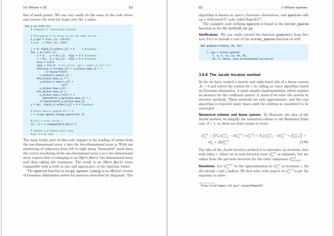
3.6 Diffusion in 2D 321
line of mesh points. We can very easily do the same in the code aboveand remove the need for loops over the i index:
for n in It[0:-1]:# Compute b, vectorized version
# Precompute f in array so we can make slicesf_a_np1 = f(xv, yv, t[n+1])f_a_n = f(xv, yv, t[n])
j = 0; b[m(0,j):m(Nx+1,j)] = 0 # Boundaryfor j in Iy[1:-1]:
i = 0; p = m(i,j); b[p] = 0 # Boundaryi = Nx; p = m(i,j); b[p] = 0 # Boundaryimin = Ix[1]imax = Ix[-1] # for slice, max i index is Ix[-1]-1b[m(imin,j):m(imax,j)] = u_n[imin:imax,j] + \
(1-theta)*(Fx*(u_n[imin+1:imax+1,j] -
2*u_n[imin:imax,j] + \u_n[imin-1:imax-1,j]) +
Fy*(u_n[imin:imax,j+1] -
2*u_n[imin:imax,j] +u_n[imin:imax,j-1])) + \
theta*dt*f_a_np1[imin:imax,j] + \(1-theta)*dt*f_a_n[imin:imax,j]
j = Ny; b[m(0,j):m(Nx+1,j)] = 0 # Boundary
# Solve matrix system A*c = bc = scipy.sparse.linalg.spsolve(A, b)
# Fill u with vector cu[:,:] = c.reshape(Ny+1,Nx+1).T
# Update u_n before next stepu_n, u = u, u_n
The most tricky part of this code snippet is the loading of values fromthe one-dimensional array c into the two-dimensional array u. With ournumbering of unknowns from left to right along “horizontal” mesh lines,the correct reordering of the one-dimensional array c as a two-dimensionalarray requires first a reshaping to an (Ny+1,Nx+1) two-dimensional arrayand then taking the transpose. The result is an (Nx+1,Ny+1) arraycompatible with u both in size and appearance of the function values.
The spsolve function in scipy.sparse.linalg is an efficient versionof Gaussian elimination suited for matrices described by diagonals. The
322 3 Diffusion equations
algorithm is known as sparse Gaussian elimination, and spsolve callsup a well-tested C code called SuperLU2.
The complete code utilizing spsolve is found in the solver_sparsefunction in the file diffu2D_u0.py.
Verification. We can easily extend the function quadratic from Sec-tion 3.6.5 to include a test of the solver_sparse function as well.
def quadratic(theta, Nx, Ny):...t, cpu = solver_sparse(
I, a, f, Lx, Ly, Nx, Ny,dt, T, theta, user_action=assert_no_error)
3.6.8 The Jacobi iterative method
So far we have created a matrix and right-hand side of a linear systemAc = b and solved the system for c by calling an exact algorithm basedon Gaussian elimination. A much simpler implementation, which requiresno memory for the coefficient matrix A, arises if we solve the system byiterative methods. These methods are only approximate, and the corealgorithm is repeated many times until the solution is considered to beconverged.
Numerical scheme and linear system. To illustrate the idea of theJacobi method, we simplify the numerical scheme to the Backward Eulercase, θ = 1, so there are fewer terms to write:
un+1i,j −
(Fx(un+1
i−1,j − 2un+1i,j + un+1
i,j ) + Fy(un+1i,j−1 − 2un+1
i,j + un+1i,j+1)
)=
uni,j +∆tfn+1i,j (3.98)
The idea of the Jacobi iterative method is to introduce an iteration, herewith index r, where we in each iteration treat un+1
i,j as unknown, but usevalues from the previous iteration for the other unknowns un+1
i±1,j±1.
Iterations. Let un+1,ri,j be the approximation to un+1
i,j in iteration r, forall relevant i and j indices. We first solve with respect to un+1
i,j to get theequation to solve:
2 http://crd-legacy.lbl.gov/ xiaoye/SuperLU/
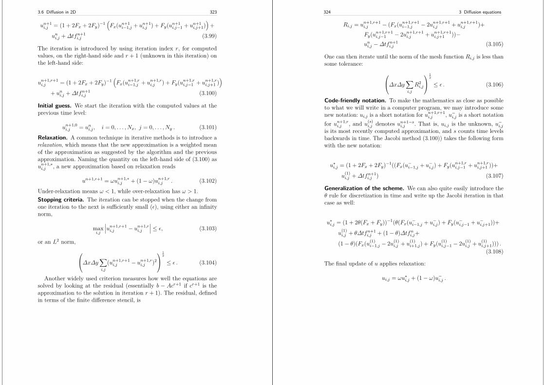
3.6 Diffusion in 2D 323
un+1i,j = (1 + 2Fx + 2Fy)−1
(Fx(un+1
i−1,j + un+1i,j ) + Fy(un+1
i,j−1 + un+1i,j+1)
)+
uni,j +∆tfn+1i,j (3.99)
The iteration is introduced by using iteration index r, for computedvalues, on the right-hand side and r + 1 (unknown in this iteration) onthe left-hand side:
un+1,r+1i,j = (1 + 2Fx + 2Fy)−1
(Fx(un+1,r
i−1,j + un+1,ri,j ) + Fy(un+1,r
i,j−1 + un+1,ri,j+1 )
)
+ uni,j +∆tfn+1i,j (3.100)
Initial guess. We start the iteration with the computed values at theprevious time level:
un+1,0i,j = uni,j , i = 0, . . . , Nx, j = 0, . . . , Ny . (3.101)
Relaxation. A common technique in iterative methods is to introduce arelaxation, which means that the new approximation is a weighted meanof the approximation as suggested by the algorithm and the previousapproximation. Naming the quantity on the left-hand side of (3.100) asun+1,∗i,j , a new approximation based on relaxation reads
un+1,r+1 = ωun+1,∗i,j + (1− ω)un+1,r
i,j . (3.102)
Under-relaxation means ω < 1, while over-relaxation has ω > 1.Stopping criteria. The iteration can be stopped when the change fromone iteration to the next is sufficiently small (ε), using either an infinitynorm,
maxi,j
∣∣∣un+1,r+1i,j − un+1,r
i,j
∣∣∣ ≤ ε, (3.103)
or an L2 norm,∆x∆y
∑
i,j
(un+1,r+1i,j − un+1,r
i,j )2
12
≤ ε . (3.104)
Another widely used criterion measures how well the equations aresolved by looking at the residual (essentially b − Acr+1 if cr+1 is theapproximation to the solution in iteration r + 1). The residual, definedin terms of the finite difference stencil, is
324 3 Diffusion equations
Ri,j = un+1,r+1i,j − (Fx(un+1,r+1
i−1,j − 2un+1,r+1i,j + un+1,r+1
i,j )+Fy(un+1,r+1
i,j−1 − 2un+1,r+1i,j + un+1,r+1
i,j+1 ))−uni,j −∆tfn+1
i,j (3.105)
One can then iterate until the norm of the mesh function Ri,j is less thansome tolerance:
∆x∆y
∑
i,j
R2i,j
12
≤ ε . (3.106)
Code-friendly notation. To make the mathematics as close as possibleto what we will write in a computer program, we may introduce somenew notation: ui,j is a short notation for un+1,r+1
i,j , u−i,j is a short notationfor un+1,r
i,j , and u(s)i,j denotes un+1−s
i,j . That is, ui,j is the unknown, u−i,jis its most recently computed approximation, and s counts time levelsbackwards in time. The Jacobi method (3.100)) takes the following formwith the new notation:
u∗i,j = (1 + 2Fx + 2Fy)−1((Fx(u−i−1,j + u−i,j) + Fy(un+1,ri,j−1 + un+1,r
i,j+1 ))+
u(1)i,j +∆tfn+1
i,j ) (3.107)
Generalization of the scheme. We can also quite easily introduce theθ rule for discretization in time and write up the Jacobi iteration in thatcase as well:
u∗i,j = (1 + 2θ(Fx + Fy))−1(θ(Fx(u−i−1,j + u−i,j) + Fy(u−i,j−1 + u−i,j+1))+
u(1)i,j + θ∆tfn+1
i,j + (1− θ)∆tfni,j+(1− θ)(Fx(u(1)
i−1,j − 2u(1)i,j + u
(1)i+1,j) + Fy(u(1)
i,j−1 − 2u(1)i,j + u
(1)i,j+1))) .(3.108)
The final update of u applies relaxation:
ui,j = ωu∗i,j + (1− ω)u−i,j .
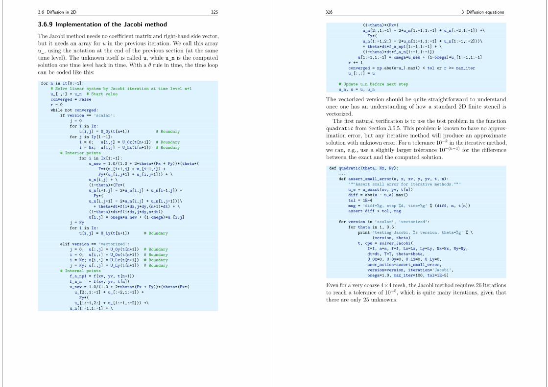
3.6 Diffusion in 2D 325
3.6.9 Implementation of the Jacobi method
The Jacobi method needs no coefficient matrix and right-hand side vector,but it needs an array for u in the previous iteration. We call this arrayu_, using the notation at the end of the previous section (at the sametime level). The unknown itself is called u, while u_n is the computedsolution one time level back in time. With a θ rule in time, the time loopcan be coded like this:
for n in It[0:-1]:# Solve linear system by Jacobi iteration at time level n+1u_[:,:] = u_n # Start valueconverged = Falser = 0while not converged:
if version == ’scalar’:j = 0for i in Ix:
u[i,j] = U_0y(t[n+1]) # Boundaryfor j in Iy[1:-1]:
i = 0; u[i,j] = U_0x(t[n+1]) # Boundaryi = Nx; u[i,j] = U_Lx(t[n+1]) # Boundary
# Interior pointsfor i in Ix[1:-1]:
u_new = 1.0/(1.0 + 2*theta*(Fx + Fy))*(theta*(Fx*(u_[i+1,j] + u_[i-1,j]) +Fy*(u_[i,j+1] + u_[i,j-1])) + \
u_n[i,j] + \(1-theta)*(Fx*(u_n[i+1,j] - 2*u_n[i,j] + u_n[i-1,j]) +
Fy*(u_n[i,j+1] - 2*u_n[i,j] + u_n[i,j-1]))\
+ theta*dt*f(i*dx,j*dy,(n+1)*dt) + \(1-theta)*dt*f(i*dx,j*dy,n*dt))u[i,j] = omega*u_new + (1-omega)*u_[i,j]
j = Nyfor i in Ix:
u[i,j] = U_Ly(t[n+1]) # Boundary
elif version == ’vectorized’:j = 0; u[:,j] = U_0y(t[n+1]) # Boundaryi = 0; u[i,:] = U_0x(t[n+1]) # Boundaryi = Nx; u[i,:] = U_Lx(t[n+1]) # Boundaryj = Ny; u[:,j] = U_Ly(t[n+1]) # Boundary
# Internal pointsf_a_np1 = f(xv, yv, t[n+1])f_a_n = f(xv, yv, t[n])u_new = 1.0/(1.0 + 2*theta*(Fx + Fy))*(theta*(Fx*(
u_[2:,1:-1] + u_[:-2,1:-1]) +Fy*(
u_[1:-1,2:] + u_[1:-1,:-2])) +\u_n[1:-1,1:-1] + \
326 3 Diffusion equations
(1-theta)*(Fx*(u_n[2:,1:-1] - 2*u_n[1:-1,1:-1] + u_n[:-2,1:-1]) +\
Fy*(u_n[1:-1,2:] - 2*u_n[1:-1,1:-1] + u_n[1:-1,:-2]))\+ theta*dt*f_a_np1[1:-1,1:-1] + \(1-theta)*dt*f_a_n[1:-1,1:-1])
u[1:-1,1:-1] = omega*u_new + (1-omega)*u_[1:-1,1:-1]r += 1converged = np.abs(u-u_).max() < tol or r >= max_iteru_[:,:] = u
# Update u_n before next stepu_n, u = u, u_n
The vectorized version should be quite straightforward to understandonce one has an understanding of how a standard 2D finite stencil isvectorized.
The first natural verification is to use the test problem in the functionquadratic from Section 3.6.5. This problem is known to have no approx-imation error, but any iterative method will produce an approximatesolution with unknown error. For a tolerance 10−k in the iterative method,we can, e.g., use a slightly larger tolerance 10−(k−1) for the differencebetween the exact and the computed solution.
def quadratic(theta, Nx, Ny):...def assert_small_error(u, x, xv, y, yv, t, n):
"""Assert small error for iterative methods."""u_e = u_exact(xv, yv, t[n])diff = abs(u - u_e).max()tol = 1E-4msg = ’diff=%g, step %d, time=%g’ % (diff, n, t[n])assert diff < tol, msg
for version in ’scalar’, ’vectorized’:for theta in 1, 0.5:
print ’testing Jacobi, %s version, theta=%g’ % \(version, theta)
t, cpu = solver_Jacobi(I=I, a=a, f=f, Lx=Lx, Ly=Ly, Nx=Nx, Ny=Ny,dt=dt, T=T, theta=theta,U_0x=0, U_0y=0, U_Lx=0, U_Ly=0,user_action=assert_small_error,version=version, iteration=’Jacobi’,omega=1.0, max_iter=100, tol=1E-5)
Even for a very coarse 4×4 mesh, the Jacobi method requires 26 iterationsto reach a tolerance of 10−5, which is quite many iterations, given thatthere are only 25 unknowns.
3.6 Diffusion in 2D 327
3.6.10 Test problem: diffusion of a sine hillIt can be shown that
ue = Ae−απ2(L−2
x +L−2y )t sin
(π
Lxx
)sin(π
Lyy
), (3.109)
is a solution of the 2D homogeneous diffusion equation ut = α(uxx + uyy)in a rectangle [0, Lx] × [0, Ly], for any value of the amplitude A. Thissolution vanishes at the boundaries, and the initial condition is theproduct of two sines. We may choose A = 1 for simplicity.
It is difficult to know if our solver based on the Jacobi method worksproperly since we are faced with two sources of errors: one from thediscretization, E∆, and one from the iterative Jacobi method, Ei. Thetotal error in the computed u can be represented as
Eu = E∆ + Ei .
One error measure is to look at the maximum value, which is obtainedfor the midpoint x = Lx/2 and y = Lx/2. This midpoint is representedin the discrete u if Nx and Ny are even numbers. We can then computeEu as Eu = |max ue−max u|, when we know an exact solution ue of theproblem.
What about E∆? If we use the maximum value as a measure of theerror, we have in fact analytical insight into the approximation error inthis particular problem. According to Section 3.3.9, the exact solution(3.109) of the PDE problem is also an exact solution of the discreteequations, except that the damping factor in time is different. Moreprecisely, (3.66) and (3.67) are solutions of the discrete problem for θ = 1(Backward Euler) and θ = 1
2 (Crank-Nicolson), respectively. The factorsraised to the power n is the numerical amplitude, and the errors in thesefactors become
E∆ = e−αk2t −
(1− 2(Fx sin2 px + Fx sin2 py)1 + 2(Fx sin2 px + Fx sin2 py)
)n, θ = 1
2 ,
E∆ = e−αk2t − (1 + 4Fx sin2 px + 4Fy sin2 py)−n, θ = 1 .
We are now in a position to compute Ei numerically. That is, we cancompute the error due to iterative solution of the linear system andsee if it corresponds to the convergence tolerance used in the method.Note that the convergence is based on measuring the difference in two
328 3 Diffusion equations
consecutive approximations, which is not exactly the error due to theiteration, but it is a kind of measure, and it should have about the samesize as Ei.
The function demo_classic_iterative in diffu2D_u0.py imple-ments the idea above (also for the methods in Section 3.6.12). Thevalue of Ei is in particular printed at each time level. By changing thetolerance in the convergence criterion in the Jacobi method, we can seethat Ei is of the same order of magnitude as the prescribed tolerancein the Jacobi method. For example: E∆ ∼ 10−2 with Nx = Ny = 10and θ = 1
2 , as long as max u has some significant size (max u > 0.02).An appropriate value of the tolerance is then 10−3, such that the errorin the Jacobi method does not become bigger than the discretizationerror. In that case, Ei is around 5 · 10−3. The corresponding numberof Jacobi iterations (with ω = 1) varies from 31 to 12 during the timesimulation (for max u > 0.02). Changing the tolerance to 10−5 causesmany more iterations (61 to 42) without giving any contribution to theoverall accuracy, because the total error is dominated by E∆.
Also, with an Nx = Ny = 20, the spatial accuracy increases and manymore iterations are needed (143 to 45), but the dominating error is fromthe time discretization. However, with such a finer spatial mesh, a highertolerance in the convergence criterion 10−4 is needed to keep Ei ∼ 10−3.More experiments show the disadvantage of the very simple Jacobiiteration method: the number of iterations increases with the numberof unknowns, keeping the tolerance fixed, but the tolerance should alsobe lowered to avoid the iteration error to dominate the total error. Asmall adjustment of the Jacobi method, as described in Section 3.6.12,provides a better method.
3.6.11 The relaxed Jacobi method and its relation to theForward Euler method
We shall now show that solving the Poisson equation −α∇2u = f by theJacobi iterative method is in fact equivalent to using a Forward Eulerscheme on ut = α∇2u+ f and letting t→∞.
A Forward Euler discretization of the 2D diffusion equation,
[D+t u = α(DxDxu+DyDyu) + f ]ni,j ,
can be written out as
3.6 Diffusion in 2D 329
un+1i,j = uni,j + ∆t
αh2
(uni−1,j + uni+1,j + uni,j−1 + uni,j+1 − 4uni,j + h2fi,j
),
where h = ∆x = ∆y has been introduced for simplicity. The scheme canbe reordered as
un+1i,j = (1− ω)uni,j+
14ω(uni−1,j + uni+1,j + uni,j−1 + uni,j+1 − 4uni,j + h2fi,j
),
with
ω = 4 ∆tαh2 ,
but this latter form is nothing but the relaxed Jacobi method applied to
[DxDxu+DyDyu = −f ]ni,j .
From the equivalence above we know a couple of things about theJacobi method for solving −∇2u = f :
1. The method is unstable if ω > 1 (since the Forward Euler method isthen unstable).
2. The convergence is really slow as the iteration index increases (comingfrom the fact that the Forward Euler scheme requires many smalltime steps to reach the stationary solution).
These observations are quite disappointing: if we already have a time-dependent diffusion problem and want to take larger time steps by animplicit time discretization method, we will with the Jacobi methodend up with something close to a slow Forward Euler simulation of theoriginal problem at each time level. Nevertheless, the are two reasonsfor why the Jacobi method remains a fundamental building block forsolving linear systems arising from PDEs: 1) a couple of iterations removelarge parts of the error and this is effectively used in the very efficientclass of multigrid methods; and 2) the idea of the Jacobi method canbe developed into more efficient methods, especially the SOR method,which is treated next.
3.6.12 The Gauss-Seidel and SOR methodsIf we update the mesh points according to the Jacobi method (3.99)for a Backward Euler discretization with a loop over i = 1, . . . , Nx − 1
330 3 Diffusion equations
and j = 1, . . . , Ny − 1, we realize that when un+1,r+1i,j is computed,
un+1,r+1i−1,j and un+1,r+1
i,j−1 are already computed, so these new values canbe used rather than un+1,r
i−1,j and un+1,ri,j−1 (respectively) in the formula for
un+1,r+1i,j . This idea gives rise to the Gauss-Seidel iteration method, which
mathematically is just a small adjustment of (3.99):
un+1,r+1i,j = (1 + 2Fx + 2Fy)−1((
Fx(un+1,r+1i−1,j + un+1,r
i,j ) + Fy(un+1,r+1i,j−1 + un+1,r
i,j+1 )) + uni,j +∆tfn+1i,j ) .(3.110)
Observe that the way we access the mesh points in the formula (3.110)is important: points with i − 1 must be computed before points withi, and points with j − 1 must be computed before points with j. Anysequence of mesh points can be used in the Gauss-Seidel method, butthe particular math formula must distinguish between already visitedpoints in the current iteration and the points not yet visited.
The idea of relaxation (3.102) can equally well be applied to the Gauss-Seidel method. Actually, the Gauss-Seidel method with an arbitrary0 < ω ≤ 2 has its own name: the Successive Over-Relaxation method,abbreviated as SOR.
The SOR method for a θ rule discretization, with the shortened u andu− notation, can be written
u∗i,j = (1 + 2θ(Fx + Fy))−1(θ(Fx(ui−1,j + u−i,j) + Fy(ui,j−1 + u−i,j+1))+
u(1)i,j + θ∆tfn+1
i,j + (1− θ)∆tfni,j+(1− θ)(Fx(u(1)
i−1,j − 2u(1)i,j + u
(1)i+1,j) + Fy(u(1)
i,j−1 − 2u(1)i,j + u
(1)i,j+1))),(3.111)
ui,j = ωu∗i,j + (1− ω)u−i,j (3.112)
The sequence of mesh points in (3.111) is i = 1, . . . , Nx − 1, j =1, . . . , Ny − 1 (but whether i runs faster or slower than j does notmatter).
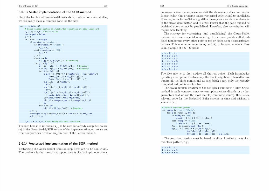
3.6 Diffusion in 2D 331
3.6.13 Scalar implementation of the SOR methodSince the Jacobi and Gauss-Seidel methods with relaxation are so similar,we can easily make a common code for the two:
for n in It[0:-1]:# Solve linear system by Jacobi/SOR iteration at time level n+1u_[:,:] = u_n # Start valueconverged = Falser = 0while not converged:
if version == ’scalar’:if iteration == ’Jacobi’:
u__ = u_elif iteration == ’SOR’:
u__ = uj = 0for i in Ix:
u[i,j] = U_0y(t[n+1]) # Boundaryfor j in Iy[1:-1]:
i = 0; u[i,j] = U_0x(t[n+1]) # Boundaryi = Nx; u[i,j] = U_Lx(t[n+1]) # Boundaryfor i in Ix[1:-1]:
u_new = 1.0/(1.0 + 2*theta*(Fx + Fy))*(theta*(Fx*(u_[i+1,j] + u__[i-1,j]) +Fy*(u_[i,j+1] + u__[i,j-1])) + \
u_n[i,j] + (1-theta)*(Fx*(
u_n[i+1,j] - 2*u_n[i,j] + u_n[i-1,j]) +Fy*(
u_n[i,j+1] - 2*u_n[i,j] + u_n[i,j-1]))\+ theta*dt*f(i*dx,j*dy,(n+1)*dt) + \
(1-theta)*dt*f(i*dx,j*dy,n*dt))u[i,j] = omega*u_new + (1-omega)*u_[i,j]
j = Nyfor i in Ix:
u[i,j] = U_Ly(t[n+1]) # boundaryr += 1converged = np.abs(u-u_).max() < tol or r >= max_iteru_[:,:] = u
u_n, u = u, u_n # Get ready for next iteration
The idea here is to introduce u__ to be used for already computed values(u) in the Gauss-Seidel/SOR version of the implementation, or just valuesfrom the previous iteration (u_) in case of the Jacobi method.
3.6.14 Vectorized implementation of the SOR methodVectorizing the Gauss-Seidel iteration step turns out to be non-trivial.The problem is that vectorized operations typically imply operations
332 3 Diffusion equations
on arrays where the sequence we visit the elements in does not matter.In particular, this principle makes vectorized code trivial to parallelize.However, in the Gauss-Seidel algorithm the sequence we visit the elementsin the arrays does matter, and it is well known that the basic method asexplained above cannot be parallelized. Therefore, also vectorization willrequire new thinking.
The strategy for vectorizing (and parallelizing) the Gauss-Seidelmethod is to use a special numbering of the mesh points called red-black numbering: every other point is red or black as in a checkerboardpattern. This numbering requires Nx and Ny to be even numbers. Hereis an example of a 6× 6 mesh:
r b r b r b rb r b r b r br b r b r b rb r b r b r br b r b r b rb r b r b r br b r b r b r
The idea now is to first update all the red points. Each formula forupdating a red point involves only the black neighbors. Thereafter, weupdate all the black points, and at each black point, only the recentlycomputed red points are involved.
The scalar implementation of the red-black numbered Gauss-Seidelmethod is really compact, since we can update values directly in u (thatguarantees that we use the most recently computed values). Here is therelevant code for the Backward Euler scheme in time and without asource term:
# Update internal pointsfor sweep in ’red’, ’black’:
for j in range(1, Ny, 1):if sweep == ’red’:
start = 1 if j % 2 == 1 else 2elif sweep == ’black’:
start = 2 if j % 2 == 1 else 1for i in range(start, Nx, 2):u[i,j] = 1.0/(1.0 + 2*(Fx + Fy))*(
Fx*(u[i+1,j] + u[i-1,j]) +Fy*(u[i,j+1] + u[i,j-1]) + u_n[i,j])
The vectorized version must be based on slices. Looking at a typicalred-black pattern, e.g.,
r b r b r b rb r b r b r br b r b r b r
3.6 Diffusion in 2D 333
b r b r b r br b r b r b rb r b r b r br b r b r b r
we want to update the internal points (marking boundary points withx):
x x x x x x xx r b r b r xx b r b r b xx r b r b r xx b r b r b xx r b r b r xx x x x x x x
It is impossible to make one slice that picks out all the internal red points.Instead, we need two slices. The first involves points marked with R:
x x x x x x xx R b R b R xx b r b r b xx R b R b R xx b r b r b xx R b R b R xx x x x x x x
This slice is specified as 1::2 for i and 1::2 for j, or with slice objects:
i = slice(1, None, 2); j = slice(1, None, 2)
The second slice involves the red points with R:
x x x x x x xx r b r b r xx b R b R b xx r b r b r xx b R b R b xx r b r b r xx x x x x x x
The slices are
i = slice(2, None, 2); j = slice(2, None, 2)
For the black points, the first slice involves the B points:
x x x x x x xx r B r B r xx b r b r b xx r B r B r xx b r b r b xx r B r B r xx x x x x x x
334 3 Diffusion equations
with slice objects
i = slice(2, None, 2); j = slice(1, None, 2)
The second set of black points is shown here:
x x x x x x xx r b r b r xx B r B r B xx r b r b r xx B r B r B xx r b r b r xx x x x x x x
with slice objects
i = slice(1, None, 2); j = slice(2, None, 2)
That is, we need four sets of slices. The simplest way of implementingthe algorithm is to make a function with variables for the slices repre-senting i, i− 1, i+ 1, j, j − 1, and j + 1, here called ic (“i center”), im1(“i minus 1”, ip1 (“i plus 1”), jc, jm1, and jp1, respectively.
def update(u_, u_n, ic, im1, ip1, jc, jm1, jp1):return \
1.0/(1.0 + 2*theta*(Fx + Fy))*(theta*(Fx*(u_[ip1,jc] + u_[im1,jc]) +Fy*(u_[ic,jp1] + u_[ic,jm1])) +\
u_n[ic,jc] + (1-theta)*(Fx*(u_n[ip1,jc] - 2*u_n[ic,jc] + u_n[im1,jc]) +\Fy*(u_n[ic,jp1] - 2*u_n[ic,jc] + u_n[ic,jm1]))+\theta*dt*f_a_np1[ic,jc] + \(1-theta)*dt*f_a_n[ic,jc])
The formula returned from update is to be compared with (3.111).The relaxed Jacobi iteration can be implemented by
ic = jc = slice(1,-1)im1 = jm1 = slice(0,-2)ip1 = jp1 = slice(2,None)u_new[ic,jc] = update(
u_, u_n, ic, im1, ip1, jc, jm1, jp1)u[ic,jc] = omega*u_new[ic,jc] + (1-omega)*u_[ic,jc]
The Gauss-Seidel (or SOR) updates need four different steps. The icand jc slices are specified above. For each of these, we must specify thecorresponding im1, ip1, jm1, and jp1 slices. The code below containsthe details.
# Red pointsic = slice(1,-1,2)im1 = slice(0,-2,2)
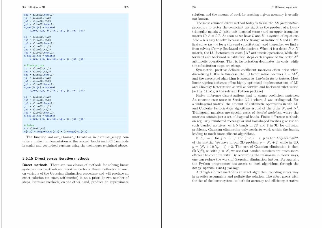
3.6 Diffusion in 2D 335
ip1 = slice(2,None,2)jc = slice(1,-1,2)jm1 = slice(0,-2,2)jp1 = slice(2,None,2)u_new[ic,jc] = update(
u_new, u_n, ic, im1, ip1, jc, jm1, jp1)
ic = slice(2,-1,2)im1 = slice(1,-2,2)ip1 = slice(3,None,2)jc = slice(2,-1,2)jm1 = slice(1,-2,2)jp1 = slice(3,None,2)u_new[ic,jc] = update(
u_new, u_n, ic, im1, ip1, jc, jm1, jp1)
# Black pointsic = slice(2,-1,2)im1 = slice(1,-2,2)ip1 = slice(3,None,2)jc = slice(1,-1,2)jm1 = slice(0,-2,2)jp1 = slice(2,None,2)u_new[ic,jc] = update(
u_new, u_n, ic, im1, ip1, jc, jm1, jp1)
ic = slice(1,-1,2)im1 = slice(0,-2,2)ip1 = slice(2,None,2)jc = slice(2,-1,2)jm1 = slice(1,-2,2)jp1 = slice(3,None,2)u_new[ic,jc] = update(
u_new, u_n, ic, im1, ip1, jc, jm1, jp1)
# Relaxc = slice(1,-1)u[c,c] = omega*u_new[c,c] + (1-omega)*u_[c,c]
The function solver_classic_iterative in diffu2D_u0.py con-tains a unified implementation of the relaxed Jacobi and SOR methodsin scalar and vectorized versions using the techniques explained above.
3.6.15 Direct versus iterative methodsDirect methods. There are two classes of methods for solving linearsystems: direct methods and iterative methods. Direct methods are basedon variants of the Gaussian elimination procedure and will produce anexact solution (in exact arithmetics) in an a priori known number ofsteps. Iterative methods, on the other hand, produce an approximate
336 3 Diffusion equations
solution, and the amount of work for reaching a given accuracy is usuallynot known.
The most common direct method today is to use the LU factorizationprocedure to factor the coefficient matrix A as the product of a lower-triangular matrix L (with unit diagonal terms) and an upper-triangularmatrix U : A = LU . As soon as we have L and U , a system of equationsLUc = b is easy to solve because of the triangular nature of L and U . Wefirst solve Ly = b for y (forward substitution), and thereafter we find cfrom solving Uc = y (backward substitution). When A is a dense N ×Nmatrix, the LU factorization costs 1
3N3 arithmetic operations, while the
forward and backward substitution steps each require of the order N2
arithmetic operations. That is, factorization dominates the costs, whilethe substitution steps are cheap.
Symmetric, positive definite coefficient matrices often arise whendiscretizing PDEs. In this case, the LU factorization becomes A = LLT ,and the associated algorithm is known as Cholesky factorization. Mostlinear algebra software offers highly optimized implementations of LUand Cholesky factorization as well as forward and backward substitution(scipy.linalg is the relevant Python package).
Finite difference discretizations lead to sparse coefficient matrices.An extreme case arose in Section 3.2.1 where A was tridiagonal. Fora tridiagonal matrix, the amount of arithmetic operations in the LUand Cholesky factorization algorithms is just of the order N , not N3.Tridiagonal matrices are special cases of banded matrices, where thematrices contain just a set of diagonal bands. Finite difference methodson regularly numbered rectangular and box-shaped meshes give rise tosuch banded matrices, with 5 bands in 2D and 7 in 3D for diffusionproblems. Gaussian elimination only needs to work within the bands,leading to much more efficient algorithms.
If Ai,j = 0 for j > i + p and j < i − p, p is the half-bandwidthof the matrix. We have in our 2D problem p = Nx + 2, while in 3D,p = (Nx + 1)(Ny + 1) + 2. The cost of Gaussian elimination is thenO(Np2), so with p N , we see that banded matrices are much moreefficient to compute with. By reordering the unknowns in clever ways,one can reduce the work of Gaussian elimination further. Fortunately,the Python programmer has access to such algorithms through thescipy.sparse.linalg package.
Although a direct method is an exact algorithm, rounding errors mayin practice accumulate and pollute the solution. The effect grows withthe size of the linear system, so both for accuracy and efficiency, iterative
3.6 Diffusion in 2D 337
methods are better suited than direct methods for solving really largelinear systems.
Iterative methods. The Jacobi and SOR iterative methods belong to aclass of iterative methods where the idea is to solve Au = b by splittingA into two parts, A = M −N , such that solving systems Mu = c is easyand efficient. With the splitting, we get a system
Mu = Nu+ b,
which suggests an iterative method
Mur+1 = Nur + b, r = 0, 1, 2, . . . ,
where ur+1 is a new approximation to u in the r + 1-th iteration. Toinitiate the iteration, we need a start vector u0.
The Jacobi and SOR methods are based on splitting A into a lowertridiagonal part L, the diagonal D, and an upper tridiagonal part U ,such that A = L+D + U . The Jacobi method corresponds to M = Dand N = −L− U . The Gauss-Seidel method employs M = L+D andN = −U , while the SOR method corresponds to
M = 1ωD + L, N = 1− ω
ωD − U .
The relaxed Jacobi method has similar expressions:
M = 1ωD, N = 1− ω
ωD − L− U .
With the matrix forms of the Jacobi and SOR methods as writtenabove, we could in an implementation alternatively fill the matrix A withentries and call general implementations of the Jacobi or SOR methodsthat work on a system Au = b. However, this is almost never donesince forming the matrix A requires quite some code and storing A inthe computer’s memory is unnecessary. It is much easier to just applythe Jacobi and SOR ideas to the finite difference stencils directly in animplementation, as we have shown in detail.
Nevertheless, the matrix formulation of the Jacobi and SOR methodshave been important for analyzing their convergence behavior. Onecan show that the error ur − u fulfills ur − u = Gr(u0 − u), whereG = M−1N and Gk is a matrix exponential. For the method to converge,limr→∞ ||Gr|| = 0 is a necessary and sufficient condition. This impliesthat the spectral radius of G must be less than one. Since G is directly
338 3 Diffusion equations
related to the finite difference scheme for the underlying PDE problem,one can in principle compute the spectral radius. For a given PDEproblem, however, this is not a practical strategy, since it is very difficultto develop useful formulas. Analysis of model problems, usually relatedto the Poisson equation, reveals some trends of interest: the convergencerate of the Jacobi method goes like h2, while that of SOR with an optimalω goes like h, where h is the spatial spacing: h = ∆x = ∆y. That is, theefficiency of the Jacobi method quickly deteriorates with the increasingmesh resolution, and SOR is much to be preferred (even if the optimalω remains an open question). We refer to Chapter 4 of [16] for moreinformation on the convergence theory. One important result is that ifA is symmetric and positive definite, then SOR will converge for any0 < ω < 2.
The optimal ω parameter can be theoretically established for a Poissonproblem as
ωo = 21 +
√1− %2 , % = cos(π/Nx) + (∆x/∆y)2 cos(π/Ny)
1 + (∆x/∆y)2 . (3.113)
This formula can be used as a guide also in other problems.The Jacobi and the SOR methods have their great advantage of
being trivial to implement, so they are obviously popular of this reason.However, the slow convergence of these methods limits the popularity tofairly small linear systems (i.e., coarse meshes). As soon as the matrixsize grows, one is better off with more sophisticated iterative methodslike the preconditioned Conjugate gradient method, which we now turnto.
Finally, we mention that there is a variant of the SOR method, calledSymmetric Successive Overrelaxation method, known as SSOR, whereone runs a standard SOR sweep through the mesh points and then a newsweep but visiting the points in reverse order.
3.6.16 The Conjugate gradient method
There is no simple intuitive derivation of the Conjugate gradient method,so we refer to the many excellent expositions in the literature for theidea of the method and how the algorithm is derived. In particular, werecommend the books [2, 1, 16, 5]. A brief overview is provided in the
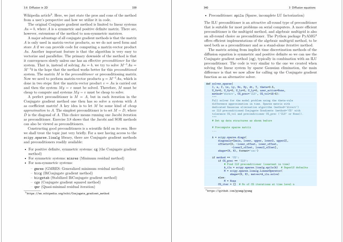
3.6 Diffusion in 2D 339
Wikipedia article3. Here, we just state the pros and cons of the methodfrom a user’s perspective and how we utilize it in code.
The original Conjugate gradient method is limited to linear systemsAu = b, where A is a symmetric and positive definite matrix. There are,however, extensions of the method to non-symmetric matrices.
A major advantage of all conjugate gradient methods is that the matrixA is only used in matrix-vector products, so we do not need form andstore A if we can provide code for computing a matrix-vector productAu. Another important feature is that the algorithm is very easy tovectorize and parallelize. The primary downside of the method is thatit convergences slowly unless one has an effective preconditioner for thesystem. That is, instead of solving Au = b, we try to solve M−1Au =M−1b in the hope that the method works better for this preconditionedsystem. The matrix M is the preconditioner or preconditioning matrix.Now we need to perform matrix-vector products y = M−1Au, which isdone in two steps: first the matrix-vector product v = Au is carried outand then the system My = v must be solved. Therefore, M must becheap to compute and systems My = v must be cheap to solve.
A perfect preconditioner is M = A, but in each iteration in theConjugate gradient method one then has so solve a system with Aas coefficient matrix! A key idea is to let M be some kind of cheapapproximation to A. The simplest preconditioner is to set M = D, whereD is the diagonal of A. This choice means running one Jacobi iterationas preconditioner. Exercise 3.8 shows that the Jacobi and SOR methodscan also be viewed as preconditioners.
Constructing good preconditioners is a scientific field on its own. Herewe shall treat the topic just very briefly. For a user having access to thescipy.sparse.linalg library, there are Conjugate gradient methodsand preconditioners readily available:
• For positive definite, symmetric systems: cg (the Conjugate gradientmethod)
• For symmetric systems: minres (Minimum residual method)• For non-symmetric systems:
– gmres (GMRES: Generalized minimum residual method)– bicg (BiConjugate gradient method)– bicgstab (Stabilized BiConjugate gradient method)– cgs (Conjugate gradient squared method)– qmr (Quasi-minimal residual iteration)
3 https://en.wikipedia.org/wiki/Conjugate_gradient_method
340 3 Diffusion equations
• Preconditioner: spilu (Sparse, incomplete LU factorization)
The ILU preconditioner is an attractive all-round type of preconditionerthat is suitable for most problems on serial computers. A more efficientpreconditioner is the multigrid method, and algebraic multigrid is alsoan all-round choice as preconditioner. The Python package PyAMG4
offers efficient implementations of the algebraic multigrid method, to beused both as a preconditioner and as a stand-alone iterative method.
The matrix arising from implicit time discretization methods of thediffusion equation is symmetric and positive definite so we can use theConjugate gradient method (cg), typically in combination with an ILUpreconditioner. The code is very similar to the one we created whensolving the linear system by sparse Gaussian elimination, the maindifference is that we now allow for calling up the Conjugate gradientfunction as an alternative solver.
def solver_sparse(I, a, f, Lx, Ly, Nx, Ny, dt, T, theta=0.5,U_0x=0, U_0y=0, U_Lx=0, U_Ly=0, user_action=None,method=’direct’, CG_prec=’ILU’, CG_tol=1E-5):"""Full solver for the model problem using the theta-ruledifference approximation in time. Sparse matrix withdedicated Gaussian elimination algorithm (method=’direct’)or ILU preconditioned Conjugate Gradients (method=’CG’ withtolerance CG_tol and preconditioner CG_prec (’ILU’ or None))."""# Set up data structures as shown before
# Precompute sparse matrix...
A = scipy.sparse.diags(diagonals=[main, lower, upper, lower2, upper2],offsets=[0, -lower_offset, lower_offset,
-lower2_offset, lower2_offset],shape=(N, N), format=’csc’)
if method == ’CG’:if CG_prec == ’ILU’:
# Find ILU preconditioner (constant in time)A_ilu = scipy.sparse.linalg.spilu(A) # SuperLU defaultsM = scipy.sparse.linalg.LinearOperator(
shape=(N, N), matvec=A_ilu.solve)else:
M = NoneCG_iter = [] # No of CG iterations at time level n
4 https://github.com/pyamg/pyamg
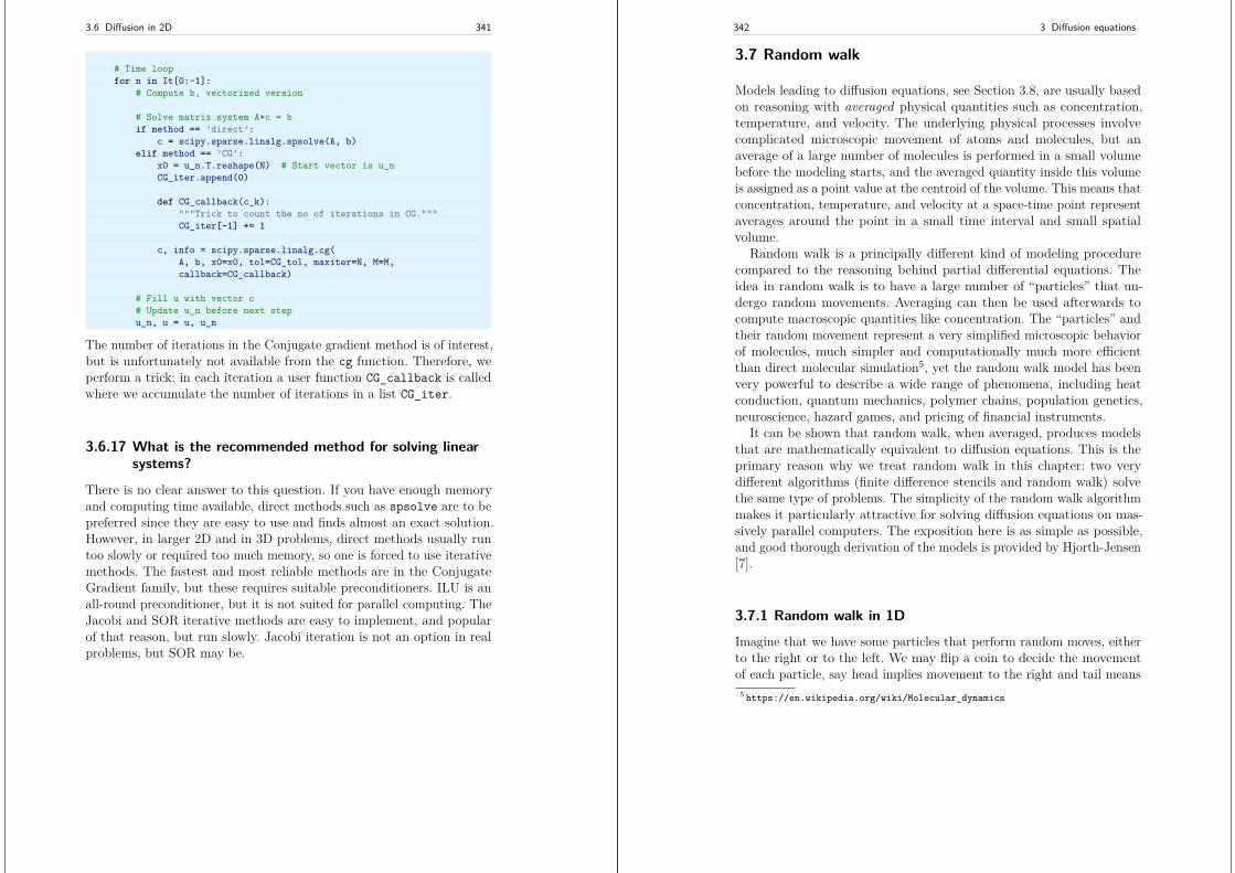
3.6 Diffusion in 2D 341
# Time loopfor n in It[0:-1]:
# Compute b, vectorized version
# Solve matrix system A*c = bif method == ’direct’:
c = scipy.sparse.linalg.spsolve(A, b)elif method == ’CG’:
x0 = u_n.T.reshape(N) # Start vector is u_nCG_iter.append(0)
def CG_callback(c_k):"""Trick to count the no of iterations in CG."""CG_iter[-1] += 1
c, info = scipy.sparse.linalg.cg(A, b, x0=x0, tol=CG_tol, maxiter=N, M=M,callback=CG_callback)
# Fill u with vector c# Update u_n before next stepu_n, u = u, u_n
The number of iterations in the Conjugate gradient method is of interest,but is unfortunately not available from the cg function. Therefore, weperform a trick: in each iteration a user function CG_callback is calledwhere we accumulate the number of iterations in a list CG_iter.
3.6.17 What is the recommended method for solving linearsystems?
There is no clear answer to this question. If you have enough memoryand computing time available, direct methods such as spsolve are to bepreferred since they are easy to use and finds almost an exact solution.However, in larger 2D and in 3D problems, direct methods usually runtoo slowly or required too much memory, so one is forced to use iterativemethods. The fastest and most reliable methods are in the ConjugateGradient family, but these requires suitable preconditioners. ILU is anall-round preconditioner, but it is not suited for parallel computing. TheJacobi and SOR iterative methods are easy to implement, and popularof that reason, but run slowly. Jacobi iteration is not an option in realproblems, but SOR may be.
342 3 Diffusion equations
3.7 Random walk
Models leading to diffusion equations, see Section 3.8, are usually basedon reasoning with averaged physical quantities such as concentration,temperature, and velocity. The underlying physical processes involvecomplicated microscopic movement of atoms and molecules, but anaverage of a large number of molecules is performed in a small volumebefore the modeling starts, and the averaged quantity inside this volumeis assigned as a point value at the centroid of the volume. This means thatconcentration, temperature, and velocity at a space-time point representaverages around the point in a small time interval and small spatialvolume.
Random walk is a principally different kind of modeling procedurecompared to the reasoning behind partial differential equations. Theidea in random walk is to have a large number of “particles” that un-dergo random movements. Averaging can then be used afterwards tocompute macroscopic quantities like concentration. The “particles” andtheir random movement represent a very simplified microscopic behaviorof molecules, much simpler and computationally much more efficientthan direct molecular simulation5, yet the random walk model has beenvery powerful to describe a wide range of phenomena, including heatconduction, quantum mechanics, polymer chains, population genetics,neuroscience, hazard games, and pricing of financial instruments.
It can be shown that random walk, when averaged, produces modelsthat are mathematically equivalent to diffusion equations. This is theprimary reason why we treat random walk in this chapter: two verydifferent algorithms (finite difference stencils and random walk) solvethe same type of problems. The simplicity of the random walk algorithmmakes it particularly attractive for solving diffusion equations on mas-sively parallel computers. The exposition here is as simple as possible,and good thorough derivation of the models is provided by Hjorth-Jensen[7].
3.7.1 Random walk in 1DImagine that we have some particles that perform random moves, eitherto the right or to the left. We may flip a coin to decide the movementof each particle, say head implies movement to the right and tail means
5 https://en.wikipedia.org/wiki/Molecular_dynamics
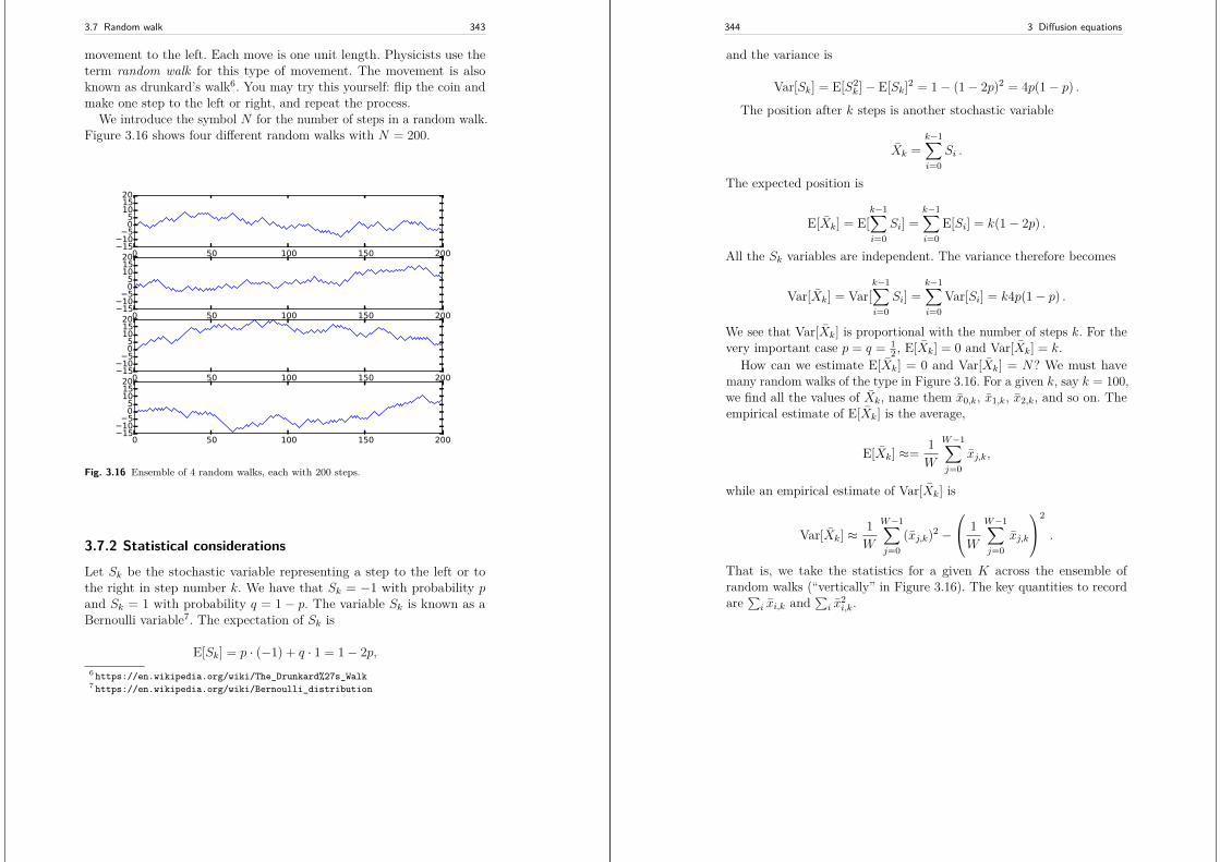
3.7 Random walk 343
movement to the left. Each move is one unit length. Physicists use theterm random walk for this type of movement. The movement is alsoknown as drunkard’s walk6. You may try this yourself: flip the coin andmake one step to the left or right, and repeat the process.
We introduce the symbol N for the number of steps in a random walk.Figure 3.16 shows four different random walks with N = 200.
0 50 100 150 2001510
505
101520
0 50 100 150 2001510
505
101520
0 50 100 150 2001510
505
101520
0 50 100 150 2001510
505
101520
Fig. 3.16 Ensemble of 4 random walks, each with 200 steps.
3.7.2 Statistical considerationsLet Sk be the stochastic variable representing a step to the left or tothe right in step number k. We have that Sk = −1 with probability pand Sk = 1 with probability q = 1 − p. The variable Sk is known as aBernoulli variable7. The expectation of Sk is
E[Sk] = p · (−1) + q · 1 = 1− 2p,6 https://en.wikipedia.org/wiki/The_Drunkard%27s_Walk7 https://en.wikipedia.org/wiki/Bernoulli_distribution
344 3 Diffusion equations
and the variance is
Var[Sk] = E[S2k ]− E[Sk]2 = 1− (1− 2p)2 = 4p(1− p) .
The position after k steps is another stochastic variable
Xk =k−1∑
i=0Si .
The expected position is
E[Xk] = E[k−1∑
i=0Si] =
k−1∑
i=0E[Si] = k(1− 2p) .
All the Sk variables are independent. The variance therefore becomes
Var[Xk] = Var[k−1∑
i=0Si] =
k−1∑
i=0Var[Si] = k4p(1− p) .
We see that Var[Xk] is proportional with the number of steps k. For thevery important case p = q = 1
2 , E[Xk] = 0 and Var[Xk] = k.How can we estimate E[Xk] = 0 and Var[Xk] = N? We must have
many random walks of the type in Figure 3.16. For a given k, say k = 100,we find all the values of Xk, name them x0,k, x1,k, x2,k, and so on. Theempirical estimate of E[Xk] is the average,
E[Xk] ≈= 1W
W−1∑
j=0xj,k,
while an empirical estimate of Var[Xk] is
Var[Xk] ≈1W
W−1∑
j=0(xj,k)2 −
1W
W−1∑
j=0xj,k
2
.
That is, we take the statistics for a given K across the ensemble ofrandom walks (“vertically” in Figure 3.16). The key quantities to recordare
∑i xi,k and
∑i x
2i,k.
3.7 Random walk 345
3.7.3 Playing around with some code
Scalar code. Python has a random module for drawing random numbers,and this module has a function uniform(a, b) for drawing a uniformlydistributed random number in the interval [a, b). If an event happenswith probability p, we can simulate this on the computer by drawing arandom number r in [0, 1), because then r ≤ p with probability p andr > p with probability 1− p:
import randomr = random.uniform(0, 1)if r <= p:
# Event happenselse:
# Event does not happen
A random walk with N steps, starting at x0, where we move to the leftwith probability p and to the right with probability 1 − p can now beimplemented by
import random, numpy as np
def random_walk1D(x0, N, p):"""1D random walk with 1 particle."""# Store position in step k in position[k]position = np.zeros(N)position[0] = x0current_pos = x0for k in range(N-1):
r = random.uniform(0, 1)if r <= p:
current_pos -= 1else:
current_pos += 1position[k+1] = current_pos
return position
Vectorized code. Since N is supposed to be large and we want to repeatthe process for many particles, we should speed up the code as much aspossible. Vectorization is the obvious technique here: we draw all the ran-dom numbers at once with aid of numpy, and then we formulate vector op-erations to get rid of the loop over the steps (k). The numpy.random mod-ule has vectorized versions of the functions in Python’s built-in randommodule. For example, numpy.random.uniform(a, b, N) returns N ran-dom numbers uniformly distributed between a (included) and b (notincluded).
346 3 Diffusion equations
We can then make an array of all the steps in a random walk: if therandom number is less than or equal to p, the step is −1, otherwise thestep is 1:
r = np.random.uniform(0, 1, size=N)steps = np.where(r <= p, -1, 1)
The value of position[k] is the sum of all steps up to step k. Suchsums are often needed in vectorized algorithms and therefore availableby the numpy.cumsum function:
>>> import numpy as np>>> np.cumsum(np.array([1,3,4,6]))array([ 1, 4, 8, 14])
The resulting array in this demo has elements 1, 1 + 3 = 4, 1 + 3 + 4 = 8,and 1 + 3 + 4 + 6 = 14.
We can now vectorize the random_walk1D function:
def random_walk1D_vec(x0, N, p):"""Vectorized version of random_walk1D."""# Store position in step k in position[k]position = np.zeros(N+1)position[0] = x0r = np.random.uniform(0, 1, size=N)steps = np.where(r <= p, -1, 1)position[1:] = x0 + np.cumsum(steps)return position
This code runs about 10 times faster than the scalar version. With aparallel numpy library, the code can also automatically take advantage ofhardware for parallel computing because each of the four array operationscan be trivially parallelized.Fixing the random sequence. During software development with ran-dom numbers it is advantageous to always generate the same sequenceof random numbers as this may help debugging processes. To fix thesequence, we set a seed of the random number generator to some choseninteger, e.g.,
np.random.seed(10)
Calls to random_walk1D_vec give positions of the particle as depictedin Figure 3.17. The particle starts at the origin and moves with p = 1
2 .Since the seed is the same, the plot to the left is just a magnification ofthe first 1,000 steps in the plot to the right.Verification. When we have a scalar and a vectorized code, it is always agood idea to develop a unit test for checking that they produce the same
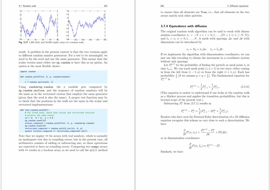
3.7 Random walk 347
0 200 400 600 800 100010
5
0
5
10
15
20
25
0 10000 20000 30000 40000 50000250
200
150
100
50
0
50
100
150
Fig. 3.17 1,000 (left) and 50,000 (right) steps of a random walk.
result. A problem in the present context is that the two versions applyto different random number generators. For a test to be meaningful, weneed to fix the seed and use the same generator. This means that thescalar version must either use np.random or have this as an option. Anoption is the most flexible choice:
import random
def random_walk1D(x0, N, p, random=random):...r = random.uniform(0, 1)
Using random=np.random, the r variable gets computed bynp.random.uniform, and the sequence of random numbers will bethe same as in the vectorized version that employs the same generator(given that the seed is also the same). A proper test function may beto check that the positions in the walk are the same in the scalar andvectorized implementations:
def test_random_walk1D():# For fixed seed, check that scalar and vectorized versions# produce the same resultx0 = 2; N = 4; p = 0.6np.random.seed(10)scalar_computed = random_walk1D(x0, N, p, random=np.random)np.random.seed(10)vectorized_computed = random_walk1D_vec(x0, N, p)assert (scalar_computed == vectorized_computed).all()
Note that we employ == for arrays with real numbers, which is normallyan inadequate test due to rounding errors, but in the present case, allarithmetics consists of adding or subtracting one, so these operationsare expected to have no rounding errors. Comparing two numpy arrayswith == results in a boolean array, so we need to call the all() method
348 3 Diffusion equations
to ensure that all elements are True, i.e., that all elements in the twoarrays match each other pairwise.
3.7.4 Equivalence with diffusionThe original random walk algorithm can be said to work with dimen-sionless coordinates xi = −N + i, i = 0, 1, . . . , 2N + 1 (i ∈ [−N,N ]),and tn = n, n = 0, 1, . . . , N . A mesh with spacings ∆x and ∆t withdimensions can be introduced by
xi = X0 + xi∆x, tn = tn∆t .
If we implement the algorithm with dimensionless coordinates, we canjust use this rescaling to obtain the movement in a coordinate systemwithout unit spacings.
Let P n+1i be the probability of finding the particle at mesh point xi at
time tn+1. We can reach mesh point (i, n+ 1) in two ways: either comingin from the left from (i − 1, n) or from the right (i + 1, n). Each hasprobability 1
2 (if we assume p = q = 12). The fundamental equation for
P n+1i is
P n+1i = 1
2Pni−1 + 1
2Pni+1 . (3.114)
(This equation is easiest to understand if one looks at the random walkas a Markov process and applies the transition probabilities, but this isbeyond scope of the present text.)
Subtracting P ni from (3.7.1) results in
P n+1i − P n
i = 12(P n
i−1 − 2P ni + 1
2Pni+1) .
Readers who have seen the Forward Euler discretization of a 1D diffusionequation recognize this scheme as very close to such a discretization. Wehave
∂
∂tP (xi, tn) = P n+1
i − P ni
∆t+O(∆t),
or in dimensionless coordinates
∂
∂tP (xi, tn) ≈ P n+1
i − P ni .
Similarly, we have
3.7 Random walk 349
∂2
∂x2P (xi, tn) =P ni−1 − 2P n
i + 12P
ni+1
∆x2 +O(∆x2),
∂2
∂x2P (xi, tn) ≈ P ni−1 − 2P n
i + 12P
ni+1 .
Equation (3.7.1) is therefore equivalent with the dimensionless diffusionequation
∂P
∂t= 1
2∂2P
∂x2 , (3.115)
or the diffusion equation
∂P
∂t= D
∂2P
∂x2 , (3.116)
with diffusion coefficient
D = ∆x2
2∆t .
This derivation shows the tight link between random walk and diffusion.If we keep track of where the particle is, and repeat the process manytimes, or run the algorithms for lots of particles, the histogram of thepositions will approximate the solution of the diffusion equation for thelocal probability P n
i .Suppose all the random walks start at the origin. Then the initial
condition for the probability distribution is the Dirac delta function δ(x).The solution of (3.115) can be shown to be
P (x, t) = 1√4παt
e−x24αt , (3.117)
where α = 12 .
3.7.5 Implementation of multiple walks
Our next task is to implement an ensemble of walks (for statistics, seeSection 3.7.2) and also provide data from the walks such that we cancompute the probabilities of the positions as introduced in the previoussection. An appropriate representation of probabilities P n
i are histograms(with i along the x axis) for a few selected values of n.
350 3 Diffusion equations
To estimate the expectation and variance of the random walks, Sec-tion 3.7.2 points to recording
∑j xj,k and
∑j x
2j,k, where xj,k is the
position at time/step level k in random walk number j. The histogramof positions needs the individual values xi,k for all i values and someselected k values.
We introduce position[k] to hold∑j xj,k, position2[k] to hold∑
j(xj,k)2, and pos_hist[i,k] to hold xi,k. A selection of k values canbe specified by saying how many, num_times, and let them be equallyspaced through time:
pos_hist_times = [(N//num_times)*i for i in range(num_times)]
This is one of the few situations we want integer division (//) or realdivision rounded to an integer.Scalar version. Our scalar implementation of running num_walks ran-dom walks may go like this:
def random_walks1D(x0, N, p, num_walks=1, num_times=1,random=random):
"""Simulate num_walks random walks from x0 with N steps."""position = np.zeros(N+1) # Accumulated positionsposition[0] = x0*num_walksposition2 = np.zeros(N+1) # Accumulated positions**2position2[0] = x0**2*num_walks# Histogram at num_times selected time pointspos_hist = np.zeros((num_walks, num_times))pos_hist_times = [(N//num_times)*i for i in range(num_times)]#print ’save hist:’, post_hist_times
for n in range(num_walks):num_times_counter = 0current_pos = x0for k in range(N):
if k in pos_hist_times:#print ’save, k:’, k, num_times_counter, npos_hist[n,num_times_counter] = current_posnum_times_counter += 1
# current_pos corresponds to step k+1r = random.uniform(0, 1)if r <= p:
current_pos -= 1else:
current_pos += 1position [k+1] += current_posposition2[k+1] += current_pos**2
return position, position2, pos_hist, np.array(pos_hist_times)
Vectorized version. We have already vectorized a single random walk.The additional challenge here is to vectorize the computation of the
3.7 Random walk 351
data for the histogram, pos_hist, but given the selected steps inpos_hist_times, we can find the corresponding positions by indexingwith the list pos_hist_times: position[post_hist_times], which areto be inserted in pos_hist[n,:].
def random_walks1D_vec1(x0, N, p, num_walks=1, num_times=1):"""Vectorized version of random_walks1D."""position = np.zeros(N+1) # Accumulated positionsposition2 = np.zeros(N+1) # Accumulated positions**2walk = np.zeros(N+1) # Positions of current walkwalk[0] = x0# Histogram at num_times selected time pointspos_hist = np.zeros((num_walks, num_times))pos_hist_times = [(N//num_times)*i for i in range(num_times)]
for n in range(num_walks):r = np.random.uniform(0, 1, size=N)steps = np.where(r <= p, -1, 1)walk[1:] = x0 + np.cumsum(steps) # Positions of this walkposition += walkposition2 += walk**2pos_hist[n,:] = walk[pos_hist_times]
return position, position2, pos_hist, np.array(pos_hist_times)
Improved vectorized version. Looking at the vectorized version above,we still have one potentially long Python loop over n. Normally,num_walks will be much larger than N. The vectorization of the loop overN certainly speeds up the program, but if we think of vectorization asalso a way to parallelize the code, all the independent walks (the n loop)can be executed in parallel. Therefore, we should include this loop aswell in the vectorized expressions, at the expense of using more memory.
We introduce the array walks to hold the N + 1 steps of all the walks:each row represents the steps in one walk.
walks = np.zeros((num_walks, N+1)) # Positions of each walkwalks[:,0] = x0
Since all the steps are independent, we can just make one long vector ofenough random numbers (N*num_walks), translate these numbers to ±1,then we reshape the array such that the steps of each walk are stored inthe rows.
r = np.random.uniform(0, 1, size=N*num_walks)steps = np.where(r <= p, -1, 1).reshape(num_walks, N)
The next step is to sum up the steps in each walk. We need thenp.cumsum function for this, with the argument axis=1 for indicating asum across the columns:
352 3 Diffusion equations
>>> a = np.arange(6).reshape(2,3)>>> aarray([[0, 1, 2],
[3, 4, 5]])>>> np.cumsum(a, axis=1)array([[ 0, 1, 3],
[ 3, 7, 12]])
Now walks can be computed by
walks[:,1:] = x0 + np.cumsum(steps, axis=1)
The position vector is the sum of all the walks. That is, we want tosum all the rows, obtained by
position = np.sum(walks, axis=0)
A corresponding expression computes the squares of the positions. Finally,we need to compute pos_hist, but that is a matter of grabbing some ofthe walks (according to pos_hist_times):
pos_hist[:,:] = walks[:,pos_hist_times]
The complete vectorized algorithm without any loop can now be summa-rized:
def random_walks1D_vec2(x0, N, p, num_walks=1, num_times=1):"""Vectorized version of random_walks1D; no loops."""position = np.zeros(N+1) # Accumulated positionsposition2 = np.zeros(N+1) # Accumulated positions**2walks = np.zeros((num_walks, N+1)) # Positions of each walkwalks[:,0] = x0# Histogram at num_times selected time pointspos_hist = np.zeros((num_walks, num_times))pos_hist_times = [(N//num_times)*i for i in range(num_times)]
r = np.random.uniform(0, 1, size=N*num_walks)steps = np.where(r <= p, -1, 1).reshape(num_walks, N)walks[:,1:] = x0 + np.cumsum(steps, axis=1)position = np.sum(walks, axis=0)position2 = np.sum(walks**2, axis=0)pos_hist[:,:] = walks[:,pos_hist_times]return position, position2, pos_hist, np.array(pos_hist_times)
What is the gain of the vectorized implementations? One importantgain is that each vectorized operation can be automatically parallelizedif one applies a parallel numpy library like Numba8. On a single CPU,however, the speed up of the vectorized operations is also significant.With N = 1, 000 and 50,000 repeated walks, the two vectorized ver-
8 http://numba.pydata.org
3.7 Random walk 353
sions run about 25 and 18 times faster than the scalar version, withrandom_walks1D_vec1 being fastest.Remark on vectorized code and parallelization. Our first attempton vectorization removed the loop over the N steps in a single walk.However, the number of walks is usually much larger than N , becauseof the need for accurate statistics. Therefore, we should rather removethe loop over all walks. It turns out, from our efficiency experiments,that the function random_walks1D_vec2 (with no loops) is slower thanrandom_walks1D_vec1. This is a bit surprising and may be explained byless efficiency in the statements involving very large arrays, containingall steps for all walks at once.
From a parallelization and improved vectorization point of view, itwould be more natural to switch the sequence of the loops in the serialcode such that the shortest loop is the outer loop:
def random_walks1D2(x0, N, p, num_walks=1, num_times=1, ...):...current_pos = x0 + np.zeros(num_walks)num_times_counter = -1
for k in range(N):if k in pos_hist_times:num_times_counter += 1store_hist = True
else:store_hist = False
for n in range(num_walks):# current_pos corresponds to step k+1r = random.uniform(0, 1)
if r <= p:current_pos[n] -= 1
else:current_pos[n] += 1
position [k+1] += current_pos[n]position2[k+1] += current_pos[n]**2if store_hist:
pos_hist[n,num_times_counter] = current_pos[n]return position, position2, pos_hist, np.array(pos_hist_times)
The vectorized version of this code, where we just vectorize the loop overn, becomes
def random_walks1D2_vec1(x0, N, p, num_walks=1, num_times=1):"""Vectorized version of random_walks1D2."""position = np.zeros(N+1) # Accumulated positionsposition2 = np.zeros(N+1) # Accumulated positions**2# Histogram at num_times selected time pointspos_hist = np.zeros((num_walks, num_times))
354 3 Diffusion equations
pos_hist_times = [(N//num_times)*i for i in range(num_times)]
current_pos = np.zeros(num_walks)current_pos[0] = x0num_times_counter = -1
for k in range(N):if k in pos_hist_times:num_times_counter += 1store_hist = True # Store histogram data for this k
else:store_hist = False
# Move all walks one stepr = np.random.uniform(0, 1, size=num_walks)steps = np.where(r <= p, -1, 1)current_pos += stepsposition[k+1] = np.sum(current_pos)position2[k+1] = np.sum(current_pos**2)if store_hist:
pos_hist[:,num_times_counter] = current_posreturn position, position2, pos_hist, np.array(pos_hist_times)
This function runs significantly faster than the random_walks1D_vec1function above, typically 1.7 times faster. The code is also more appro-priate in a parallel computing context since each vectorized statementcan work with data of size num_walks over the compute units, repeatedN times (compared with data of size N, repeated num_walks times, inrandom_walks1D_vec1).
The scalar code with switched loops, random_walks1D2 runs a bitslower than the original code in random_walks1D, so with the longestloop as the inner loop, the vectorized function random_walks1D2_vec1is almost 60 times faster than the scalar counterpart, while the coderandom_walks1D_vec2 without loops is only around 18 times faster.Taking into account the very large arrays required by the latter function,we end up with random_walks1D2_vec1 as the preferred implementation.Test function. During program development, it is highly recommendedto carry out computations by hand for, e.g., N=4 and num_walks=3.Normally, this is done by executing the program with these parametersand checking with pen and paper that the computations make sense. Thenext step is to use this test for correctness in a formal test function.
First, we need to check that the simulation of multiple random walksreproduces the results of random_walk1D, random_walk1D_vec1, andrandom_walk1D_vec2 for the first walk, if the seed is the same. Second,we run three random walks (N=4) with the scalar and the two vectorizedversions and check that the returned arrays are identical.
3.7 Random walk 355
For this type of test to be successful, we must be sure that exactly thesame set of random numbers are used in the three versions, a fact thatrequires the same random number generator and the same seed, of course,but also the same sequence of computations. This is not obviously the casewith the three random_walk1D* functions we have presented. The criticalissue in random_walk1D_vec1 is that the first random numbers are usedfor the first walk, the second set of random numbers is used for the secondwalk and so, to be compatible with how the random numbers are usedin the function random_walk1D. For the function random_walk1D_vec2the situation is a bit more complicated since we generate all the randomnumbers at once. However, the critical step now is the reshaping of thearray returned from np.where: we must reshape as (num_walks, N) toensure that the first N random numbers are used for the first walk, thenext N numbers are used for the second walk, and so on.
We arrive at the test function below.
def test_random_walks1D():# For fixed seed, check that scalar and vectorized versions# produce the same resultx0 = 0; N = 4; p = 0.5
# First, check that random_walks1D for 1 walk reproduces# the walk in random_walk1Dnum_walks = 1np.random.seed(10)computed = random_walks1D(
x0, N, p, num_walks, random=np.random)np.random.seed(10)expected = random_walk1D(
x0, N, p, random=np.random)assert (computed[0] == expected).all()
# Same for vectorized versionsnp.random.seed(10)computed = random_walks1D_vec1(x0, N, p, num_walks)np.random.seed(10)expected = random_walk1D_vec(x0, N, p)assert (computed[0] == expected).all()np.random.seed(10)computed = random_walks1D_vec2(x0, N, p, num_walks)np.random.seed(10)expected = random_walk1D_vec(x0, N, p)assert (computed[0] == expected).all()
# Second, check multiple walks: scalar == vectorizednum_walks = 3num_times = Nnp.random.seed(10)serial_computed = random_walks1D(
356 3 Diffusion equations
x0, N, p, num_walks, num_times, random=np.random)np.random.seed(10)vectorized1_computed = random_walks1D_vec1(
x0, N, p, num_walks, num_times)np.random.seed(10)vectorized2_computed = random_walks1D_vec2(
x0, N, p, num_walks, num_times)# positions: [0, 1, 0, 1, 2]# Can test without tolerance since everything is +/- 1return_values = [’pos’, ’pos2’, ’pos_hist’, ’pos_hist_times’]for s, v, r in zip(serial_computed,
vectorized1_computed,return_values):
msg = ’%s: %s (serial) vs %s (vectorized)’ % (r, s, v)assert (s == v).all(), msg
for s, v, r in zip(serial_computed,vectorized2_computed,return_values):
msg = ’%s: %s (serial) vs %s (vectorized)’ % (r, s, v)assert (s == v).all(), msg
Such test functions are indispensable for further development of the codeas we can at any time test whether the basic computations remain corrector not. This is particularly important in stochastic simulations sincewithout test functions and fixed seeds, we always experience variationsfrom run to run, and it can be very difficult to spot bugs through averagedstatistical quantities.
3.7.6 Demonstration of multiple walksAssuming now that the code works, we can just scale up the number ofsteps in each walk and the number of walks. The latter influences theaccuracy of the statistical estimates. Figure 3.18 shows the impact ofthe number of walks on the expectation, which should approach zero.Figure 3.19 displays the corresponding estimate of the variance of theposition, which should grow linearly with the number of steps. It does,seemingly very accurately, but notice that the scale on the y axis is somuch larger than for the expectation, so irregularities due to the stochasticnature of the process become so much less visible in the variance plots.The probability of finding a particle at a certain position at time (orstep) 800 is shown in Figure 3.20. The dashed red line is the theoreticaldistribution (3.117) arising from solving the diffusion equation (3.115)instead. As always, we realize that one needs significantly more statisticalsamples to estimate a histogram accurately than the expectation orvariance.
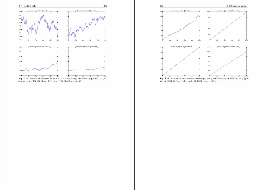
3.7 Random walk 357
0 200 400 600 800 10003.5
3.0
2.5
2.0
1.5
1.0
0.5
0.0
0.5 Expected position (100 walks)
0 200 400 600 800 10000.1
0.0
0.1
0.2
0.3
0.4
0.5 Expected position (10000 walks)
0 200 400 600 800 10000.1
0.0
0.1
0.2
0.3
0.4
0.5 Expected position (100000 walks)
0 200 400 600 800 10000.1
0.0
0.1
0.2
0.3
0.4
0.5 Expected position (1000000 walks)
Fig. 3.18 Estimated expected value for 1000 steps, using 100 walks (upper left), 10,000(upper right), 100,000 (lower left), and 1,000,000 (lower right).
358 3 Diffusion equations
0 200 400 600 800 10000
200
400
600
800
1000
1200 Variance of position (100 walks)
0 200 400 600 800 10000
200
400
600
800
1000 Variance of position (10000 walks)
0 200 400 600 800 10000
200
400
600
800
1000 Variance of position (100000 walks)
0 200 400 600 800 10000
200
400
600
800
1000
1200 Variance of position (1000000 walks)
Fig. 3.19 Estimated variance over 1000 steps, using 100 walks (upper left), 10,000 (upperright), 100,000 (lower left), and 1,000,000 (lower right).
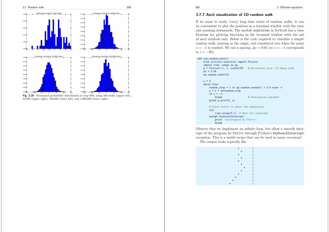
3.7 Random walk 359
100 80 60 40 20 0 20 40 600.000
0.005
0.010
0.015
0.020
0.025 Histogram of positions (100 walks)
150 100 50 0 50 100 1500.000
0.002
0.004
0.006
0.008
0.010
0.012
0.014
0.016 Histogram of positions (10000 walks)
150 100 50 0 50 100 1500.000
0.002
0.004
0.006
0.008
0.010
0.012
0.014
0.016 Histogram of positions (100000 walks)
150 100 50 0 50 100 1500.000
0.002
0.004
0.006
0.008
0.010
0.012
0.014
0.016 Histogram of positions (1000000 walks)
Fig. 3.20 Estimated probability distribution at step 800, using 100 walks (upper left),10,000 (upper right), 100,000 (lower left), and 1,000,000 (lower right).
360 3 Diffusion equations
3.7.7 Ascii visualization of 1D random walk
If we want to study (very) long time series of random walks, it canbe convenient to plot the position in a terminal window with the timeaxis pointing downwards. The module avplotter in SciTools has a classPlotter for plotting functions in the terminal window with the aidof ascii symbols only. Below is the code required to visualize a simplerandom walk, starting at the origin, and considered over when the pointx = −1 is reached. We use a spacing ∆x = 0.05 (so x = −1 correspondsto i = −20).
def run_random_walk():from scitools.avplotter import Plotterimport time, numpy as npp = Plotter(-1, 1, width=75) # Horizontal axis: 75 chars widedx = 0.05np.random.seed(10)
x = 0while True:
random_step = 1 if np.random.random() > 0.5 else -1x = x + dx*random_stepif x < -1:
break # Destination reached!print p.plot(0, x)
# Allow Ctrl+c to abort the simulationtry:
time.sleep(0.1) # Wait for interruptexcept KeyboardInterrupt:
print ’Interrupted by Ctrl+c’break
Observe that we implement an infinite loop, but allow a smooth inter-rupt of the program by Ctrl+c through Python’s KeyboardInterruptexception. This is a useful recipe that can be used in many occasions!
The output looks typically like
* |* |
* |* |
* |* |
* |* |
* |* |
* |* |
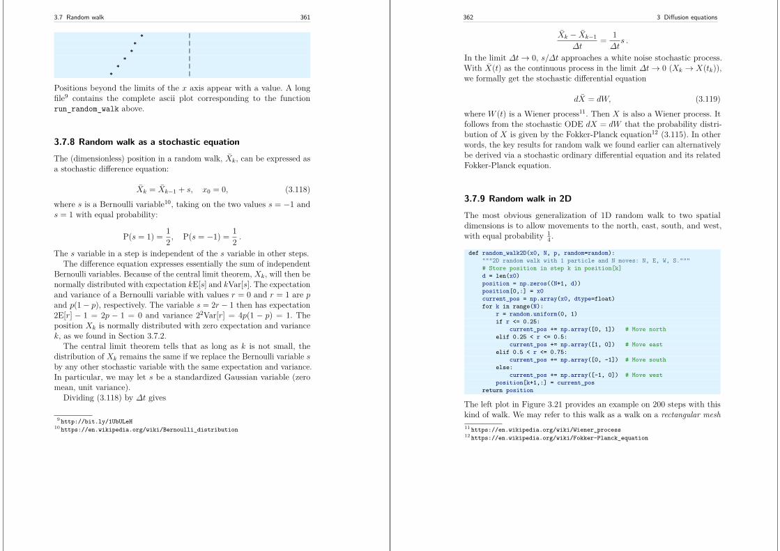
3.7 Random walk 361
* |* |
* |* |
* |* |
Positions beyond the limits of the x axis appear with a value. A longfile9 contains the complete ascii plot corresponding to the functionrun_random_walk above.
3.7.8 Random walk as a stochastic equation
The (dimensionless) position in a random walk, Xk, can be expressed asa stochastic difference equation:
Xk = Xk−1 + s, x0 = 0, (3.118)
where s is a Bernoulli variable10, taking on the two values s = −1 ands = 1 with equal probability:
P(s = 1) = 12 , P(s = −1) = 1
2 .
The s variable in a step is independent of the s variable in other steps.The difference equation expresses essentially the sum of independent
Bernoulli variables. Because of the central limit theorem, Xk, will then benormally distributed with expectation kE[s] and kVar[s]. The expectationand variance of a Bernoulli variable with values r = 0 and r = 1 are pand p(1− p), respectively. The variable s = 2r − 1 then has expectation2E[r] − 1 = 2p − 1 = 0 and variance 22Var[r] = 4p(1 − p) = 1. Theposition Xk is normally distributed with zero expectation and variancek, as we found in Section 3.7.2.
The central limit theorem tells that as long as k is not small, thedistribution of Xk remains the same if we replace the Bernoulli variable sby any other stochastic variable with the same expectation and variance.In particular, we may let s be a standardized Gaussian variable (zeromean, unit variance).
Dividing (3.118) by ∆t gives
9 http://bit.ly/1UbULeH10 https://en.wikipedia.org/wiki/Bernoulli_distribution
362 3 Diffusion equations
Xk − Xk−1∆t
= 1∆t
s .
In the limit ∆t→ 0, s/∆t approaches a white noise stochastic process.With X(t) as the continuous process in the limit ∆t→ 0 (Xk → X(tk)),we formally get the stochastic differential equation
dX = dW, (3.119)
where W (t) is a Wiener process11. Then X is also a Wiener process. Itfollows from the stochastic ODE dX = dW that the probability distri-bution of X is given by the Fokker-Planck equation12 (3.115). In otherwords, the key results for random walk we found earlier can alternativelybe derived via a stochastic ordinary differential equation and its relatedFokker-Planck equation.
3.7.9 Random walk in 2D
The most obvious generalization of 1D random walk to two spatialdimensions is to allow movements to the north, east, south, and west,with equal probability 1
4 .
def random_walk2D(x0, N, p, random=random):"""2D random walk with 1 particle and N moves: N, E, W, S."""# Store position in step k in position[k]d = len(x0)position = np.zeros((N+1, d))position[0,:] = x0current_pos = np.array(x0, dtype=float)for k in range(N):
r = random.uniform(0, 1)if r <= 0.25:
current_pos += np.array([0, 1]) # Move northelif 0.25 < r <= 0.5:
current_pos += np.array([1, 0]) # Move eastelif 0.5 < r <= 0.75:
current_pos += np.array([0, -1]) # Move southelse:
current_pos += np.array([-1, 0]) # Move westposition[k+1,:] = current_pos
return position
The left plot in Figure 3.21 provides an example on 200 steps with thiskind of walk. We may refer to this walk as a walk on a rectangular mesh11 https://en.wikipedia.org/wiki/Wiener_process12 https://en.wikipedia.org/wiki/Fokker-Planck_equation
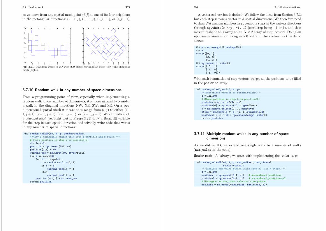
3.7 Random walk 363
as we move from any spatial mesh point (i, j) to one of its four neighborsin the rectangular directions: (i+ 1, j), (i− 1, j), (i, j + 1), or (i, j − 1).
4 2 0 2 4 6 8 1010
8
6
4
2
0
2
4
12 10 8 6 4 2 0 2 4 62
0
2
4
6
8
10
Fig. 3.21 Random walks in 2D with 200 steps: rectangular mesh (left) and diagonalmesh (right).
3.7.10 Random walk in any number of space dimensions
From a programming point of view, especially when implementing arandom walk in any number of dimensions, it is more natural to considera walk in the diagonal directions NW, NE, SW, and SE. On a two-dimensional spatial mesh it means that we go from (i, j) to either (i+1, j + 1), (i− 1, j + 1), (i+ 1, j − 1), or (i− 1, j − 1). We can with sucha diagonal mesh (see right plot in Figure 3.21) draw a Bernoulli variablefor the step in each spatial direction and trivially write code that worksin any number of spatial directions:
def random_walkdD(x0, N, p, random=random):"""Any-D (diagonal) random walk with 1 particle and N moves."""# Store position in step k in position[k]d = len(x0)position = np.zeros((N+1, d))position[0,:] = x0current_pos = np.array(x0, dtype=float)for k in range(N):
for i in range(d):r = random.uniform(0, 1)if r <= p:
current_pos[i] -= 1else:
current_pos[i] += 1position[k+1,:] = current_pos
return position
364 3 Diffusion equations
A vectorized version is desired. We follow the ideas from Section 3.7.3,but each step is now a vector in d spatial dimensions. We therefore needto draw Nd random numbers in r, compute steps in the various directionsthrough np.where(r <=p, -1, 1) (each step being −1 or 1), and thenwe can reshape this array to an N × d array of step vectors. Doing annp.cumsum summation along axis 0 will add the vectors, as this demoshows:
>>> a = np.arange(6).reshape(3,2)>>> aarray([[0, 1],
[2, 3],[4, 5]])
>>> np.cumsum(a, axis=0)array([[ 0, 1],
[ 2, 4],[ 6, 9]])
With such summation of step vectors, we get all the positions to be filledin the position array:
def random_walkdD_vec(x0, N, p):"""Vectorized version of random_walkdD."""d = len(x0)# Store position in step k in position[k]position = np.zeros((N+1,d))position[0] = np.array(x0, dtype=float)r = np.random.uniform(0, 1, size=N*d)steps = np.where(r <= p, -1, 1).reshape(N,d)position[1:,:] = x0 + np.cumsum(steps, axis=0)return position
3.7.11 Multiple random walks in any number of spacedimensions
As we did in 1D, we extend one single walk to a number of walks(num_walks in the code).
Scalar code. As always, we start with implementing the scalar case:
def random_walksdD(x0, N, p, num_walks=1, num_times=1,random=random):
"""Simulate num_walks random walks from x0 with N steps."""d = len(x0)position = np.zeros((N+1, d)) # Accumulated positionsposition2 = np.zeros((N+1, d)) # Accumulated positions**2# Histogram at num_times selected time pointspos_hist = np.zeros((num_walks, num_times, d))
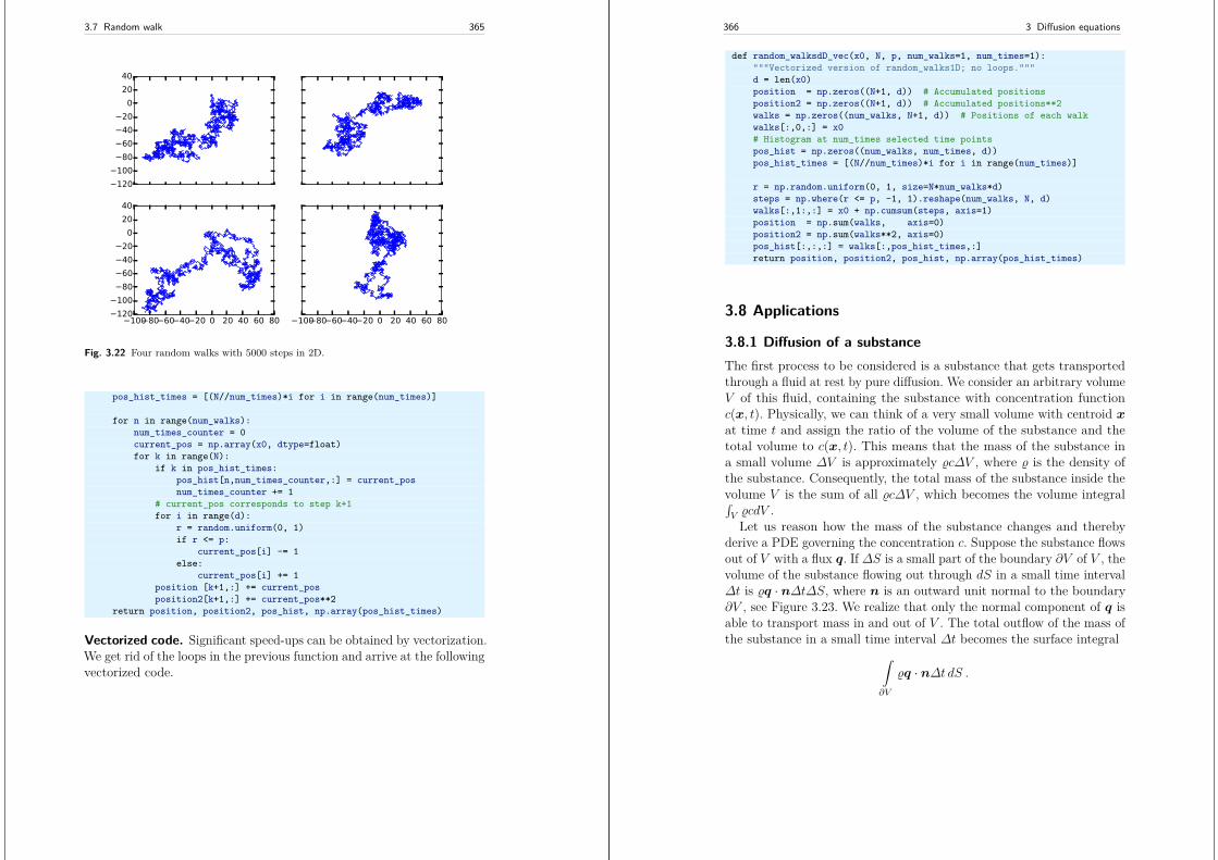
3.7 Random walk 365
120100
806040200
2040
100 80 60 40 20 0 20 40 60 80120100
806040200
2040
100 80 60 40 20 0 20 40 60 80
Fig. 3.22 Four random walks with 5000 steps in 2D.
pos_hist_times = [(N//num_times)*i for i in range(num_times)]
for n in range(num_walks):num_times_counter = 0current_pos = np.array(x0, dtype=float)for k in range(N):
if k in pos_hist_times:pos_hist[n,num_times_counter,:] = current_posnum_times_counter += 1
# current_pos corresponds to step k+1for i in range(d):
r = random.uniform(0, 1)if r <= p:
current_pos[i] -= 1else:
current_pos[i] += 1position [k+1,:] += current_posposition2[k+1,:] += current_pos**2
return position, position2, pos_hist, np.array(pos_hist_times)
Vectorized code. Significant speed-ups can be obtained by vectorization.We get rid of the loops in the previous function and arrive at the followingvectorized code.
366 3 Diffusion equations
def random_walksdD_vec(x0, N, p, num_walks=1, num_times=1):"""Vectorized version of random_walks1D; no loops."""d = len(x0)position = np.zeros((N+1, d)) # Accumulated positionsposition2 = np.zeros((N+1, d)) # Accumulated positions**2walks = np.zeros((num_walks, N+1, d)) # Positions of each walkwalks[:,0,:] = x0# Histogram at num_times selected time pointspos_hist = np.zeros((num_walks, num_times, d))pos_hist_times = [(N//num_times)*i for i in range(num_times)]
r = np.random.uniform(0, 1, size=N*num_walks*d)steps = np.where(r <= p, -1, 1).reshape(num_walks, N, d)walks[:,1:,:] = x0 + np.cumsum(steps, axis=1)position = np.sum(walks, axis=0)position2 = np.sum(walks**2, axis=0)pos_hist[:,:,:] = walks[:,pos_hist_times,:]return position, position2, pos_hist, np.array(pos_hist_times)
3.8 Applications
3.8.1 Diffusion of a substanceThe first process to be considered is a substance that gets transportedthrough a fluid at rest by pure diffusion. We consider an arbitrary volumeV of this fluid, containing the substance with concentration functionc(x, t). Physically, we can think of a very small volume with centroid xat time t and assign the ratio of the volume of the substance and thetotal volume to c(x, t). This means that the mass of the substance ina small volume ∆V is approximately %c∆V , where % is the density ofthe substance. Consequently, the total mass of the substance inside thevolume V is the sum of all %c∆V , which becomes the volume integral∫V %cdV .Let us reason how the mass of the substance changes and thereby
derive a PDE governing the concentration c. Suppose the substance flowsout of V with a flux q. If ∆S is a small part of the boundary ∂V of V , thevolume of the substance flowing out through dS in a small time interval∆t is %q · n∆t∆S, where n is an outward unit normal to the boundary∂V , see Figure 3.23. We realize that only the normal component of q isable to transport mass in and out of V . The total outflow of the mass ofthe substance in a small time interval ∆t becomes the surface integral
∫
∂V
%q · n∆t dS .
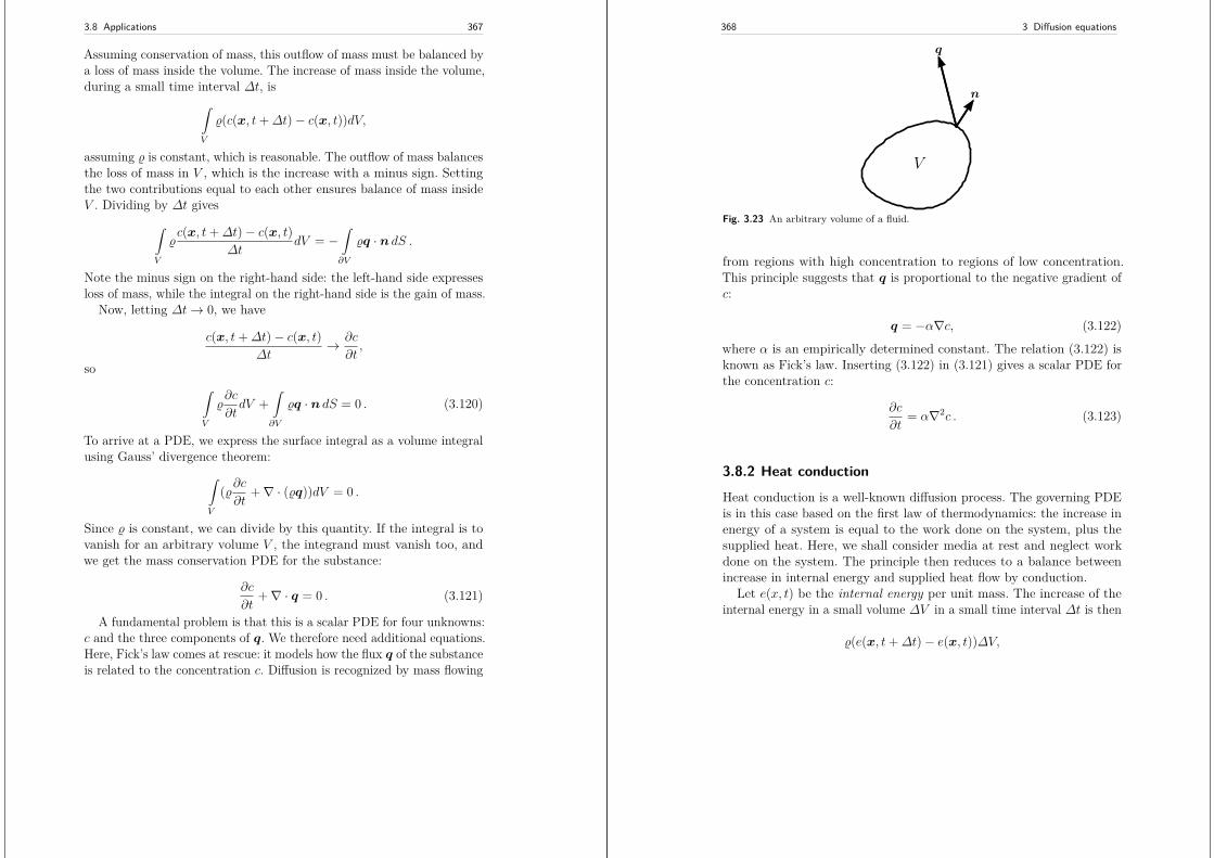
3.8 Applications 367
Assuming conservation of mass, this outflow of mass must be balanced bya loss of mass inside the volume. The increase of mass inside the volume,during a small time interval ∆t, is
∫
V
%(c(x, t+∆t)− c(x, t))dV,
assuming % is constant, which is reasonable. The outflow of mass balancesthe loss of mass in V , which is the increase with a minus sign. Settingthe two contributions equal to each other ensures balance of mass insideV . Dividing by ∆t gives
∫
V
%c(x, t+∆t)− c(x, t)
∆tdV = −
∫
∂V
%q · n dS .
Note the minus sign on the right-hand side: the left-hand side expressesloss of mass, while the integral on the right-hand side is the gain of mass.
Now, letting ∆t→ 0, we have
c(x, t+∆t)− c(x, t)∆t
→ ∂c
∂t,
so∫
V
%∂c
∂tdV +
∫
∂V
%q · n dS = 0 . (3.120)
To arrive at a PDE, we express the surface integral as a volume integralusing Gauss’ divergence theorem:
∫
V
(%∂c∂t
+∇ · (%q))dV = 0 .
Since % is constant, we can divide by this quantity. If the integral is tovanish for an arbitrary volume V , the integrand must vanish too, andwe get the mass conservation PDE for the substance:
∂c
∂t+∇ · q = 0 . (3.121)
A fundamental problem is that this is a scalar PDE for four unknowns:c and the three components of q. We therefore need additional equations.Here, Fick’s law comes at rescue: it models how the flux q of the substanceis related to the concentration c. Diffusion is recognized by mass flowing
368 3 Diffusion equations
q
V
n
Fig. 3.23 An arbitrary volume of a fluid.
from regions with high concentration to regions of low concentration.This principle suggests that q is proportional to the negative gradient ofc:
q = −α∇c, (3.122)
where α is an empirically determined constant. The relation (3.122) isknown as Fick’s law. Inserting (3.122) in (3.121) gives a scalar PDE forthe concentration c:
∂c
∂t= α∇2c . (3.123)
3.8.2 Heat conduction
Heat conduction is a well-known diffusion process. The governing PDEis in this case based on the first law of thermodynamics: the increase inenergy of a system is equal to the work done on the system, plus thesupplied heat. Here, we shall consider media at rest and neglect workdone on the system. The principle then reduces to a balance betweenincrease in internal energy and supplied heat flow by conduction.
Let e(x, t) be the internal energy per unit mass. The increase of theinternal energy in a small volume ∆V in a small time interval ∆t is then
%(e(x, t+∆t)− e(x, t))∆V,
3.8 Applications 369
where % is the density of the material subject to heat conduction. Inan arbitrary volume V , as depicted in Figure 3.23, the correspondingincrease in internal energy becomes the volume integral
∫
V
%(e(x, t+∆t)− e(x, t))dV .
This increase in internal energy is balanced by heat supplied by conduc-tion. Let q be the heat flow per time unit. Through the surface ∂V of Vthe following amount of heat flows out of V during a time interval ∆t:
∫
∂V
q · n∆t dS .
The simplified version of the first law of thermodynamics then statesthat
∫
V
%(e(x, t+∆t)− e(x, t))dV = −∫
∂V
q · n∆t dS .
The minus sign on the right-hand side ensures that the integral theremodels net inflow of heat (since n is an outward unit normal, q · nmodels outflow). Dividing by ∆t and notifying that
lim∆t→0
e(x, t+∆t)− e(x, t)∆t
= ∂e
∂t,
we get (in the limit ∆t→ 0)∫
V
%∂e
∂tdV +
∫
∂V
q · n∆t dS = 0 .
This is the integral equation for heat conduction, but we aim at a PDE.The next step is therefore to transform the surface integral to a volumeintegral via Gauss’ divergence theorem. The result is
∫
V
(%∂e
∂t+∇ · q
)dV = 0 .
If this equality is to hold for all volumes V , the integrand must vanish,and we have the PDE
%∂e
∂t= −∇ · q . (3.124)
370 3 Diffusion equations
Sometimes the supplied heat can come from the medium itself. This isthe case, for instance, when radioactive rock generates heat. Let us addthis effect. If f(x, t) is the supplied heat per unit volume per unit time,the heat supplied in a small volume is f∆t∆V , and inside an arbitraryvolume V the supplied generated heat becomes
∫
V
f∆tdV .
Adding this to the integral statement of the (simplified) first law ofthermodynamics, and continuing the derivation, leads to the PDE
%∂e
∂t= −∇ · q + f . (3.125)
There are four unknown scalar fields: e and q. Moreover, the tempera-ture T , which is our primary quantity to compute, does not enter themodel yet. We need an additional equation, called the equation of state,relating e, V = 1/% =, and T : e = e(V, T ). By the chain rule we have
∂e
∂t= ∂e
∂T
∣∣∣∣V
∂T
∂t+ ∂e
∂V
∣∣∣∣T
∂V
∂t.
The first coefficient ∂e/∂T is called specific heat capacity at constantvolume, denoted by cv:
cv = ∂e
∂T
∣∣∣∣V
.
The specific heat capacity will in general vary with T , but taking it as aconstant is a good approximation in many applications.
The term ∂e/∂V models effects due to compressibility and volumeexpansion. These effects are often small and can be neglected. We shalldo so here. Using ∂e/∂t = cv∂T/∂t in the PDE gives
%cv∂T
∂t= −∇ · q + f .
We still have four unknown scalar fields (T and q). To close the system,we need a relation between the heat flux q and the temperature T calledFourier’s law:
q = −k∇T,
3.8 Applications 371
which simply states that heat flows from hot to cold areas, along the pathof greatest variation. In a solid medium, k depends on the material ofthe medium, and in multi-material media one must regard k as spatiallydependent. In a fluid, it is common to assume that k is constant. Thevalue of k reflects how easy heat is conducted through the medium, andk is named the coefficient of heat conduction.
We have now one scalar PDE for the unknown temperature fieldT (x, t):
%cv∂T
∂t= ∇ · (k∇T ) + f . (3.126)
3.8.3 Porous media flow
The requirement of mass balance for flow of a single, incompressible fluidthrough a deformable (elastic) porous medium leads to the equation
S∂p
∂t+∇ · (q − α∂u
∂t) = 0,
where p is the fluid pressure, q is the fluid velocity, u is the displacement(deformation) of the medium, S is the storage coefficient of the medium(related to the compressibility of the fluid and the material in the medium),and α is another coefficient. In many circumstances, the last term withu can be neglected, an assumption that decouples the equation abovefrom a model for the deformation of the medium. The famous Darcy’slaw relates q to p:
q = −Kµ
(∇p− %g),
where K is the permeability of the medium, µ is the dynamic viscosityof the fluid, % is the density of the fluid, and g is the acceleration ofgravity, here taken as g = −gk. Combining the two equations results inthe diffusion model
S∂p
∂t= µ−1∇(K∇p) + %g
µ
∂K
∂z. (3.127)
Boundary conditions consist of specifying p or q · n at (normal velocity)each point of the boundary.
372 3 Diffusion equations
3.8.4 Potential fluid flow
Let v be the velocity of a fluid. The condition ∇ × v = 0 is relevantfor many flows, especially in geophysics when viscous effects are negli-gible. From vector calculus it is known that ∇× v = 0 implies that vcan be derived from a scalar potential field φ: v = ∇φ. If the fluid isincompressible, ∇ · v = 0, it follows that ∇ · ∇φ = 0, or
∇2φ = 0 . (3.128)
This Laplace equation is sufficient for determining φ and thereby describethe fluid motion. This type of flow is known as potential flow13. Onevery important application where potential flow is a good model is waterwaves. As boundary condition we must prescribe v · n = ∂φ/∂n. Thisgives rise to what is known as a pure Neumann problem and will causenumerical difficulties because φ and φ plus any constant are two solutionsof the problem. The simplest remedy is to fix the value of φ at a point.
3.8.5 Streamlines for 2D fluid flow
The streamlines in a two-dimensional stationary fluid flow are linestangential to the flow. The stream function14 ψ is often introduced intwo-dimensional flow such that its contour lines, ψ = const, gives thestreamlines. The relation between ψ and the velocity field v = (u, v) is
u = ∂ψ
∂y, v = −∂ψ
∂x.
It follows that ∇v = ψyx − ψxy = 0, so the stream function can only beused for incompressible flows. Since
∇× v =(∂v
∂y− ∂u
∂x
)k ≡ ωk,
we can derive the relation
∇2ψ = −ω, (3.129)
which is a governing equation for the stream function ψ(x, y) if thevorticity ω is known.13 https://en.wikipedia.org/wiki/Potential_flow14 https://en.wikipedia.org/wiki/Stream_function
3.8 Applications 373
3.8.6 The potential of an electric field
Under the assumption of time independence, Maxwell’s equations for theelectric field E become
∇ ·E = ρ
ε0,
∇×E = 0,
where ρ is the electric charge density and ε0 is the electric permittivityof free space (i.e., vacuum). Since ∇×E = 0, E can be derived from apotential ϕ, E = −∇ϕ. The electric field potential is therefore governedby the Poisson equation
∇2ϕ = − ρε0. (3.130)
If the medium is heterogeneous, ρ will depend on the spatial locationr. Also, ε0 must be exchanged with an electric permittivity function ε(r).
Each point of the boundary must be accompanied by, either a Dirichletcondition ϕ(r) = ϕD(r), or a Neumann condition ∂ϕ(r)
∂n = ϕN (r).
3.8.7 Development of flow between two flat plates
Diffusion equations may also arise as simplified versions of other mathe-matical models, especially in fluid flow. Consider a fluid flowing betweentwo flat, parallel plates. The velocity is uni-directional, say along the zaxis, and depends only on the distance x from the plates; u = u(x, t)k.The flow is governed by the Navier-Stokes equations,
%∂u
∂t+ %u · ∇u = −∇p+ µ∇2u+ %f ,
∇ · u = 0,
where p is the pressure field, unknown along with the velocity u, % isthe fluid density, µ the dynamic viscosity, and f is some external bodyforce. The geometric restrictions of flow between two flat plates putsrestrictions on the velocity, u = u(x, t)i, and the z component of theNavier-Stokes equations collapses to a diffusion equation:
374 3 Diffusion equations
%∂u
∂t= −∂p
∂z+ µ
∂2u
∂z2 + %fz,
if fz is the component of f in the z direction.The boundary conditions are derived from the fact that the fluid sticks
to the plates, which means u = 0 at the plates. Say the location of theplates are z = 0 and z = L. We then have
u(0, t) = u(L, t) = 0 .
One can easily show that ∂p/∂z must be a constant or just a functionof time t. We set ∂p/∂z = −β(t). The body force could be a componentof gravity, if desired, set as fz = γg. Switching from z to x as independentvariable gives a very standard one-dimensional diffusion equation:
%∂u
∂t= µ
∂2u
∂z2 + β(t) + %γg, x ∈ [0, L], t ∈ (0, T ] .
The boundary conditions are
u(0, t) = u(L, t) = 0,
while some initial condition
u(x, 0) = I(x)
must also be prescribed.The flow is driven by either the pressure gradient β or gravity, or a
combination of both. One may also consider one moving plate that drivesthe fluid. If the plate at x = L moves with velocity UL(t), we have theadjusted boundary condition
u(L, t) = UL(t) .
3.8.8 Flow in a straight tube
Now we consider viscous fluid flow in a straight tube with radius R andrigid walls. The governing equations are the Navier-Stokes equations, butas in Section 3.8.7, it is natural to assume that the velocity is directedalong the tube, and that it is axi-symmetric. These assumptions reducedthe velocity field to u = u(r, x, t)i, if the x axis is directed along thetube. From the equation of continuity, ∇ · u = 0, we see that u must be
3.8 Applications 375
independent of x. Inserting u = u(r, t)i in the Navier-Stokes equations,expressed in axi-symmetric cylindrical coordinates, results in
%∂u
∂t= µ
1r
∂
∂r
(r∂u
∂r
)+ β(t) + %γg, r ∈ [0, R], t ∈ (0, T ] . (3.131)
Here, β(t) = −∂p/∂x is the pressure gradient along the tube. Theassociated boundary condition is u(R, t) = 0.
3.8.9 Tribology: thin film fluid flow
Thin fluid films are extremely important inside machinery to reducefriction between gliding surfaces. The mathematical model for the fluidmotion takes the form of a diffusion problem and is quickly derivedhere. We consider two solid surfaces whose distance is described by agap function h(x, y). The space between these surfaces is filled with afluid with dynamic viscosity µ. The fluid may move partially because ofpressure gradients and partially because the surfaces move. Let Ui+ V jbe the relative velocity of the two surfaces and p the pressure in thefluid. The mathematical model builds on two principles: 1) conservationof mass, 2) assumption of locally quasi-static flow between flat plates.
The conservation of mass equation reads ∇ · u, where u is the localfluid velocity. For thin films the detailed variation between the surfacesis not of interest, so ∇ · u = 0 is integrated (average) in the directionperpendicular to the surfaces. This gives rise to the alternative massconservation equation
∇ · q = 0, q =h(x,y)∫
0
udz,
where z is the coordinate perpendicular to the surfaces, and q is thenthe volume flux in the fluid gap.
Locally, we may assume that we have steady flow between two flatsurfaces, with a pressure gradient and where the lower surface is atrest and the upper moves with velocity Ui + V j. The correspondingmathematical problem is actually the limit problem in Section 3.8.7 ast → ∞. The limit problem can be solved analytically, and the localvolume flux becomes
376 3 Diffusion equations
q(x, y, z) =h∫
0
u(x, y, z)dz = − h3
12µ∇p+ 12Uhi+ 1
2V hj .
The idea is to use this expression locally also when the surfaces arenot flat, but slowly varying, and if U , V , or p varies in time, providedthe time variation is sufficiently slow. This is a common quasi-staticapproximation much used in mathematical modeling.
Inserting the expression for q via p, U , and V in the equation ∇q = 0gives a diffusion PDE for p:
∇ ·(h3
12µ∇p)
= 12∂
∂x(hU) + 1
2∂
∂x(hV ) . (3.132)
The boundary conditions must involve p or q at the boundary.
3.8.10 Propagation of electrical signals in the brain
One can make a model of how electrical signals are propagated alongthe neuronal fibers that receive synaptic inputs in the brain. The signalpropagation is one-dimensional and can, in the simplest cases, be governedby the Cable equation15:
cm∂V
∂t= 1rl
∂2V
∂x2 −1rmV (3.133)
where V (x, t) is the voltage to be determined, cm is capacitance of theneuronal fiber, while rl and rm are measures of the resistance. Theboundary conditions are often taken as V = 0 at a short circuit oropen end, ∂V/∂x = 0 at a sealed end, or ∂V/∂x ∝ V where there is aninjection of current.
3.9 Exercises
Exercise 3.6: Stabilizing the Crank-Nicolson method byRannacher time stepping
It is well known that the Crank-Nicolson method may give rise to non-physical oscillations in the solution of diffusion equations if the initial data15 http://en.wikipedia.org/wiki/Cable_equation
3.9 Exercises 377
exhibit jumps (see Section 3.3.6). Rannacher [15] suggested a stabilizingtechnique consisting of using the Backward Euler scheme for the first twotime steps with step length 1
2∆t. One can generalize this idea to taking2m time steps of size 1
2∆t with the Backward Euler method and thencontinuing with the Crank-Nicolson method, which is of second-orderin time. The idea is that the high frequencies of the initial solutionare quickly damped out, and the Backward Euler scheme treats thesehigh frequencies correctly. Thereafter, the high frequency content of thesolution is gone and the Crank-Nicolson method will do well.
Test this idea for m = 1, 2, 3 on a diffusion problem with a discontinu-ous initial condition. Measure the convergence rate using the solution(3.45) with the boundary conditions (3.46)-(3.47) for t values such that theconditions are in the vicinity of ±1. For example, t < 5a1.6 · 10−2 makesthe solution diffusion from a step to almost a straight line. The programdiffu_erf_sol.py shows how to compute the analytical solution.
Project 3.7: Energy estimates for diffusion problems
This project concerns so-called energy estimates for diffusion problemsthat can be used for qualitative analytical insight and for verification ofimplementations.
a) We start with a 1D homogeneous diffusion equation with zero Dirichletconditions:
ut = αuxx,x ∈ Ω = (0, L), t ∈ (0, T ], (3.134)u(0, t) = u(L, t) = 0, t ∈ (0, T ], (3.135)
u(x, 0) = I(x), x ∈ [0, L] . (3.136)
The energy estimate for this problem reads
||u||L2 ≤ ||I||L2 , (3.137)
where the || · ||L2 norm is defined by
||g||L2 =√∫ L
0g2dx . (3.138)
378 3 Diffusion equations
The quantify ||u||L2 or 12 ||u||L2 is known as the energy of the solution,
although it is not the physical energy of the system. A mathematicaltradition has introduced the notion energy in this context.
The estimate (3.137) says that the “size of u” never exceeds that ofthe initial condition, or more precisely, it says that the area under the ucurve decreases with time.
To show (3.137), multiply the PDE by u and integrate from 0 to L.Use that uut can be expressed as the time derivative of u2 and that uxxucan integrated by parts to form an integrand u2
x. Show that the timederivative of ||u||2L2 must be less than or equal to zero. Integrate thisexpression and derive (3.137).
b) Now we address a slightly different problem,
ut = αuxx+ f(x, t),x ∈ Ω = (0, L), t ∈ (0, T ], (3.139)u(0, t) = u(L, t) = 0, t ∈ (0, T ], (3.140)
u(x, 0) = 0, x ∈ [0, L] . (3.141)
The associated energy estimate is
||u||L2 ≤ ||f ||L2 . (3.142)
(This result is more difficult to derive.)Now consider the compound problem with an initial condition I(x)
and a right-hand side f(x, t):
ut = αuxx+ f(x, t),x ∈ Ω = (0, L), t ∈ (0, T ], (3.143)u(0, t) = u(L, t) = 0, t ∈ (0, T ], (3.144)
u(x, 0) = I(x), x ∈ [0, L] . (3.145)
Show that if w1 fulfills (3.134)-(3.136) and w2 fulfills (3.139)-(3.141),then u = w1 + w2 is the solution of (3.143)-(3.145). Using the triangleinequality for norms,
||a+ b|| ≤ ||a||+ ||b||,show that the energy estimate for (3.143)-(3.145) becomes
||u||L2 ≤ ||I||L2 + ||f ||L2 . (3.146)
3.9 Exercises 379
c) One application of (3.146) is to prove uniqueness of the solution.Suppose u1 and u2 both fulfill (3.143)-(3.145). Show that u = u1 − u2then fulfills (3.143)-(3.145) with f = 0 and I = 0. Use (3.146) to deducethat the energy must be zero for all times and therefore that u1 = u2,which proves that the solution is unique.
d) Generalize (3.146) to a 2D/3D diffusion equation ut = ∇ · (α∇u) forx ∈ Ω.
Hint. Use integration by parts in multi dimensions:∫
Ωu∇ · (α∇u) dx = −
∫
Ωα∇u · ∇u dx+
∫
∂Ωuα
∂u
∂n,
where ∂u∂n = n · ∇u, n being the outward unit normal to the boundary
∂Ω of the domain Ω.
e) Now we also consider the multi-dimensional PDE ut = ∇ · (α∇u).Integrate both sides over Ω and use Gauss’ divergence theorem,
∫Ω∇ ·
q dx =∫∂Ω q ·n ds for a vector field q. Show that if we have homogeneous
Neumann conditions on the boundary, ∂u/∂n = 0, area under the usurface remains constant in time and
∫
Ωu dx =
∫
ΩI dx . (3.147)
f) Establish a code in 1D, 2D, or 3D that can solve a diffusion equationwith a source term f , initial condition I, and zero Dirichlet or Neumannconditions on the whole boundary.
We can use (3.146) and (3.147) as a partial verification of the code.Choose some functions f and I and check that (3.146) is obeyed at anytime when zero Dirichlet conditions are used. Iterate over the same Ifunctions and check that (3.147) is fulfilled when using zero Neumannconditions.
g) Make a list of some possible bugs in the code, such as indexing errorsin arrays, failure to set the correct boundary conditions, evaluation ofa term at a wrong time level, and similar. For each of the bugs, see ifthe verification tests from the previous subexercise pass or fail. Thisinvestigation shows how strong the energy estimates and the estimate(3.147) are for pointing out errors in the implementation.Filename: diffu_energy.
380 3 Diffusion equations
Exercise 3.8: Splitting methods and preconditioning
In Section 3.6.15, we outlined a class of iterative methods for Au = bbased on splitting A into A = M −N and introducing the iteration
Muk = Nuk + b .
The very simplest splitting is M = I, where I is the identity matrix.Show that this choice corresponds to the iteration
uk = uk−1 + rk−1, rk−1 = b− Auk−1, (3.148)
where rk−1 is the residual in the linear system in iteration k − 1. Theformula (3.148) is known as Richardson’s iteration. Show that if weapply the simple iteration method (3.148) to the preconditioned systemM−1Au = M−1b, we arrive at the Jacobi method by choosing M = D(the diagonal of A) as preconditioner and the SOR method by choosingM = ω−1D+L (L being the lower triangular part of A). This equivalenceshows that we can apply one iteration of the Jacobi or SOR method aspreconditioner.
Problem 3.9: Oscillating surface temperature of the earth
Consider a day-and-night or seasonal variation in temperature at thesurface of the earth. How deep down in the ground will the surfaceoscillations reach? For simplicity, we model only the vertical variationalong a coordinate x, where x = 0 at the surface, and x increases aswe go down in the ground. The temperature is governed by the heatequation
%cv∂T
∂t= ∇ · (k∇T ),
in some spatial domain x ∈ [0, L], where L is chosen large enough suchthat we can assume that T is approximately constant, independent ofthe surface oscillations, for x > L. The parameters %, cv, and k arethe density, the specific heat capacity at constant volume, and the heatconduction coefficient, respectively.
a) Derive the mathematical model for computing T (x, t). Assume thesurface oscillations to be sinusoidal around some mean temperature Tm.Let T = Tm initially. At x = L, assume T ≈ Tm.
3.9 Exercises 381
b) Scale the model in a) assuming k is constant. Use a time scaletc = ω−1 and a length scale xc =
√2α/ω, where α = k/(%cv). The
primary unknown can be scaled as T−Tm2A .
Show that the scaled PDE is
∂u
∂t= 1
2∂2u
∂x2 ,
with initial condition u(x, 0) = 0, left boundary condition u(0, t) =sin(t), and right boundary condition u(L, t) = 0. The bar indicates adimensionless quantity.
Show that u(x, t) = e−x sin(x− t) is a solution that fulfills the PDE andthe boundary condition at x = 0 (this is the solution we will experienceas t→∞ and L→∞). Conclude that an appropriate domain for x is[0, 4] if a damping e−4 ≈ 0.18 is appropriate for implementing u ≈ const;increasing to [0, 6] damps u to 0.0025.
c) Compute the scaled temperature and make animations comparingtwo solutions with L = 4 and L = 8, respectively (keep ∆x the same).
Problem 3.10: Oscillating and pulsating flow in tubes
We consider flow in a straight tube with radius R and straight walls. Theflow is driven by a pressure gradient β(t). The effect of gravity can beneglected. The mathematical problem reads
%∂u
∂t= µ
1r
∂
∂r
(r∂u
∂r
)+ β(t), r ∈ [0, R], t ∈ (0, T ], (3.149)
u(r, 0) = I(r), r ∈ [0, R], (3.150)u(R, t) = 0, t ∈ (0, T ], (3.151)∂u
∂r(0, t) = 0, t ∈ (0, T ]. (3.152)
We consider two models for β(t). One plain, sinusoidal oscillation:
β = A sin(ωt), (3.153)
and one with periodic pulses,
β = A sin16(ωt), (3.154)
382 3 Diffusion equations
Note that both models can be written as β = A sinm(ωt), with m = 1and m = 16, respectively.a) Scale the mathematical model, using the viscous time scale %R2/µ.b) Implement the scaled model from a), using the unifying θ scheme intime and centered differences in space.c) Verify the implementation in b) using a manufactured solution thatis quadratic in r and linear in t. Make a corresponding test function.Hint. You need to include an extra source term in the equation to allowfor such tests. Let the spatial variation be 1− r2 such that the boundarycondition is fulfilled.d) Make animations for m = 1, 16 and α = 1, 0.1. Choose T such thatthe motion has reached a steady state (non-visible changes from periodto period in u).e) For α 1, the scaling in a) is not good, because the characteristictime for changes (due to the pressure) is much smaller than the viscousdiffusion time scale (α becomes large). We should in this case base theshort time scale on 1/ω. Scale the model again, and make an animationfor m = 1, 16 and α = 10.Filename: axisymm_flow.
Problem 3.11: Scaling a welding problemWelding equipment makes a very localized heat source that moves in time.We shall investigate the heating due to welding and choose, for maximumsimplicity, a one-dimensional heat equation with a fixed temperatureat the ends, and we neglect melting. We shall scale the problem, andbesides solving such a problem numerically, the aim is to investigate theappropriateness of alternative scalings.
The governing PDE problem reads
%c∂u
∂t= k
∂2u
∂x2 + f,x ∈ (0, L), t ∈ (0, T ),
u(x, 0) = Us, x ∈ [0, L],u(0, t) = u(L, t) = 0, t ∈ (0, T ].
Here, u is the temperature, % the density of the material, c a heat capacity,k the heat conduction coefficient, f is the heat source from the welding
3.9 Exercises 383
equipment, and Us is the initial constant (room) temperature in thematerial.
A possible model for the heat source is a moving Gaussian function:
f = A exp(−1
2
(x− vtσ
)2),
where A is the strength, σ is a parameter governing how peak-shaped (orlocalized in space) the heat source is, and v is the velocity (in positive xdirection) of the source.
a) Let xc, tc, uc, and fc be scales, i.e., characteristic sizes, of x, t, u, andf , respectively. The natural choice of xc and fc is L and A, since thesemake the scaled x and f in the interval [0, 1]. If each of the three termsin the PDE are equally important, we can find tc and uc by demandingthat the coefficients in the scaled PDE are all equal to unity. Performthis scaling. Use scaled quantities in the arguments for the exponentialfunction in f too and show that
f = e−12β
2(x−γt)2,
where β and γ are dimensionless numbers. Give an interpretation of βand γ.
b) Argue that for large γ we should base the time scale on the movementof the heat source. Show that this gives rise to the scaled PDE
∂u
∂t= γ−1∂
2u
∂x2 + f ,
and
f = exp (−12β
2(x− t)2) .
Discuss when the scalings in a) and b) are appropriate.
c) One aim with scaling is to get a solution that lies in the interval[−1, 1]. This is not always the case when uc is based on a scale involvinga source term, as we do in a) and b). However, from the scaled PDE werealize that if we replace f with δf , where δ is a dimensionless factor,this corresponds to replacing uc by uc/δ. So, if we observe that u ∼ 1/δin simulations, we can just replace f by δf in the scaled PDE.
Use this trick and implement the two scaled models. Reusesoftware for the diffusion equation (e.g., the solver function in
384 3 Diffusion equations
diffu1D_vc.py). Make a function run(gamma, beta=10, delta=40,scaling=1, animate=False) that runs the model with the given γ,β, and δ parameters as well as an indicator scaling that is 1 for thescaling in a) and 2 for the scaling in b). The last argument can be usedto turn screen animations on or off.
Experiments show that with γ = 1 and β = 10, δ = 20 is appropriate.Then max |u| will be larger than 4 for γ = 40, but that is acceptable.
Equip the run function with visualization, both animation of u and f ,and plots with u and f for t = 0.2 and t = 0.5.
Hint. Since the amplitudes of u and f differs by a factor δ, it is attractiveto plot f/δ together with u.
d) Use the software in c) to investigate γ = 0.2, 1, 5, 40 for the twoscalings. Discuss the results.Filename: welding.
Exercise 3.12: Implement a Forward Euler scheme foraxi-symmetric diffusion
Based on the discussion in Section 3.5.6, derive in detail the discreteequations for a Forward Euler in time, centered in space, finite differencemethod for axi-symmetric diffusion. The diffusion coefficient may bea function of the radial coordinate. At the outer boundary r = R, wemay have either a Dirichlet or Robin condition. Implement this scheme.Construct appropriate test problems.Filename: FE_axisym.
Advection-dominated equations 4
Wave (Chapter 2) and diffusion (Chapter 3) equations are solved reliablyby finite difference methods. As soon as we add a first-order deriva-tive in space, representing advective transport, also known as convectivetransport, the numerics gets more complicated, and intuitively attractivemethods no longer work well. We shall show how and why such methodsfail and provide remedies. The present chapter builds on basic knowl-edge about finite difference methods for diffusion and wave equations,including the analysis by Fourier components, truncation error analysis(Appendix B), and compact difference notation.
Remark on terminology
It is common to refer to movement of a fluid as convection, whileadvection is the transport of some material dissolved or suspendedin the fluid. We shall mostly choose the word advection here, butboth terms are in heavy use, and for mass transport of a substancethe PDE has an advection term, while the similar term for the heatequation is a convection term.
Much more comprehensive discussion of dispersion analysis for ad-vection problems can be found in the book by Duran [3]. This is a anexcellent resource for further studies on the topic of advection PDEs,with emphasis on generalizations to real geophysical problems. The book
© 2016, Hans Petter Langtangen, Svein Linge. Released under CC Attribution 4.0 license
386 4 Advection-dominated equations
by Fletcher [4] also has a good overview of methods for advection andconvection problems.
4.1 One-dimensional time-dependent advectionequations
We consider the pure advection model
∂u
∂t+ v
∂u
∂x= 0, x ∈ (0, L), t ∈ (0, T ], (4.1)
u(x, 0) = I(x), x ∈ (0, L), (4.2)u(0, t) = U0, t ∈ (0, T ]. (4.3)
In (4.1), v is a given parameter, typically reflecting the velocity oftransport of a quantity u with a flow. There is only one boundarycondition (4.2) since the spatial derivative is only first order in the PDE(4.1). The information at x = 0 and the initial condition get transportedin the positive x direction if v > 0 through the domain.
It is easiest to find the solution of (4.1) if we remove the boundarycondition and consider a process on the infinite domain (−∞,∞). Thesolution is simply
u(x, t) = I(x− vt) . (4.4)
This is also the solution we expect locally in a finite domain beforeboundary conditions have reflected or modified the wave.
A particular feature of the solution (4.4) is that
u(xi, tn+1) = u(xi−1, tn), (4.5)
if xi = i∆x and tn = n∆t are points in a uniform mesh. We see thisrelation from
u(i∆x, (n+1)∆t) = I(i∆x−v(n+1)∆t) = I((i−1)∆x−vn∆t−v∆t−∆x) = I((i−1)∆x−vn∆t) = u((i−1)∆x, n∆t),
provided v = ∆x/∆t. So, whenever we see a scheme that collapses to
un+1i = uni−1, (4.6)
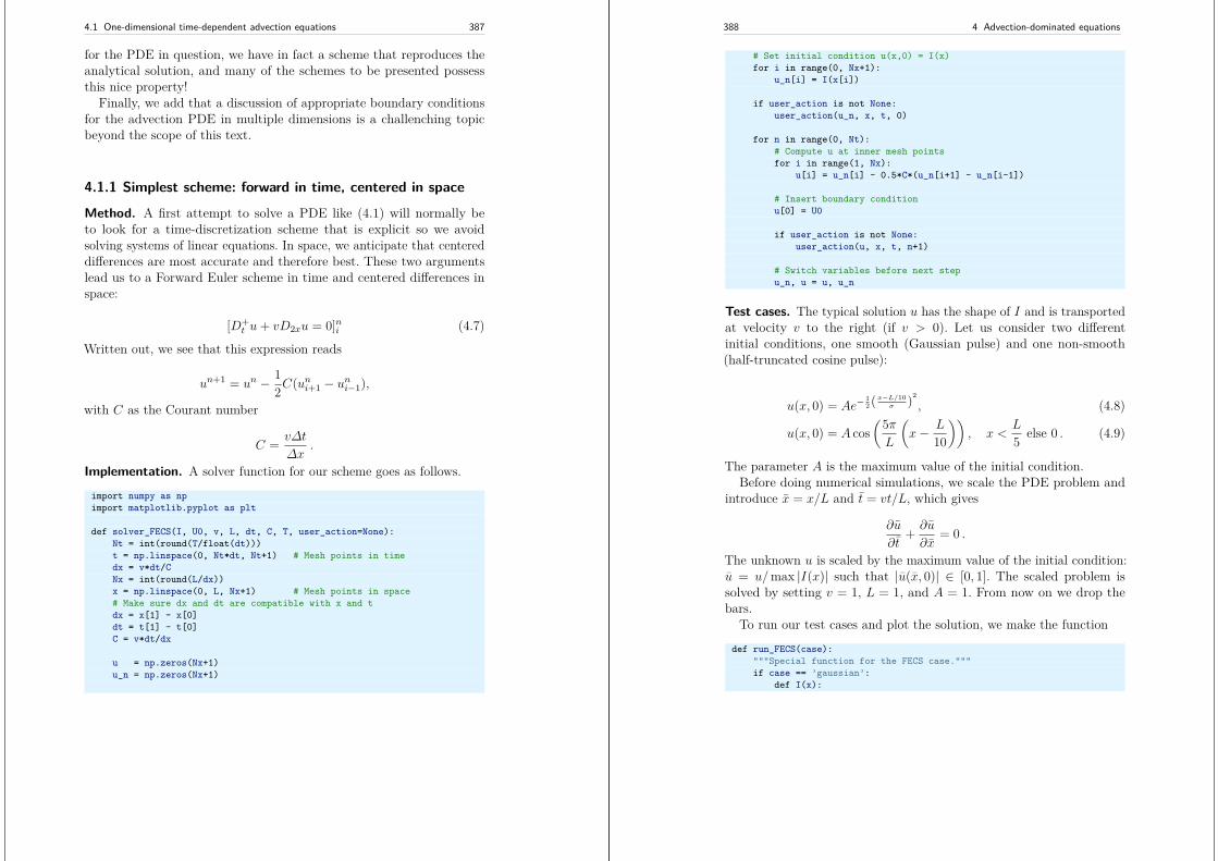
4.1 One-dimensional time-dependent advection equations 387
for the PDE in question, we have in fact a scheme that reproduces theanalytical solution, and many of the schemes to be presented possessthis nice property!
Finally, we add that a discussion of appropriate boundary conditionsfor the advection PDE in multiple dimensions is a challenching topicbeyond the scope of this text.
4.1.1 Simplest scheme: forward in time, centered in space
Method. A first attempt to solve a PDE like (4.1) will normally beto look for a time-discretization scheme that is explicit so we avoidsolving systems of linear equations. In space, we anticipate that centereddifferences are most accurate and therefore best. These two argumentslead us to a Forward Euler scheme in time and centered differences inspace:
[D+t u+ vD2xu = 0]ni (4.7)
Written out, we see that this expression reads
un+1 = un − 12C(uni+1 − uni−1),
with C as the Courant number
C = v∆t
∆x.
Implementation. A solver function for our scheme goes as follows.
import numpy as npimport matplotlib.pyplot as plt
def solver_FECS(I, U0, v, L, dt, C, T, user_action=None):Nt = int(round(T/float(dt)))t = np.linspace(0, Nt*dt, Nt+1) # Mesh points in timedx = v*dt/CNx = int(round(L/dx))x = np.linspace(0, L, Nx+1) # Mesh points in space# Make sure dx and dt are compatible with x and tdx = x[1] - x[0]dt = t[1] - t[0]C = v*dt/dx
u = np.zeros(Nx+1)u_n = np.zeros(Nx+1)
388 4 Advection-dominated equations
# Set initial condition u(x,0) = I(x)for i in range(0, Nx+1):
u_n[i] = I(x[i])
if user_action is not None:user_action(u_n, x, t, 0)
for n in range(0, Nt):# Compute u at inner mesh pointsfor i in range(1, Nx):
u[i] = u_n[i] - 0.5*C*(u_n[i+1] - u_n[i-1])
# Insert boundary conditionu[0] = U0
if user_action is not None:user_action(u, x, t, n+1)
# Switch variables before next stepu_n, u = u, u_n
Test cases. The typical solution u has the shape of I and is transportedat velocity v to the right (if v > 0). Let us consider two differentinitial conditions, one smooth (Gaussian pulse) and one non-smooth(half-truncated cosine pulse):
u(x, 0) = Ae−12 ( x−L/10
σ )2
, (4.8)
u(x, 0) = A cos(5πL
(x− L
10
)), x <
L
5 else 0 . (4.9)
The parameter A is the maximum value of the initial condition.Before doing numerical simulations, we scale the PDE problem and
introduce x = x/L and t = vt/L, which gives
∂u
∂t+ ∂u
∂x= 0 .
The unknown u is scaled by the maximum value of the initial condition:u = u/max |I(x)| such that |u(x, 0)| ∈ [0, 1]. The scaled problem issolved by setting v = 1, L = 1, and A = 1. From now on we drop thebars.
To run our test cases and plot the solution, we make the function
def run_FECS(case):"""Special function for the FECS case."""if case == ’gaussian’:
def I(x):
4.1 One-dimensional time-dependent advection equations 389
return np.exp(-0.5*((x-L/10)/sigma)**2)elif case == ’cosinehat’:
def I(x):return np.cos(np.pi*5/L*(x - L/10)) if x < L/5 else 0
L = 1.0sigma = 0.02legends = []
def plot(u, x, t, n):"""Animate and plot every m steps in the same figure."""plt.figure(1)if n == 0:
lines = plot(x, u)else:
lines[0].set_ydata(u)plt.draw()#plt.savefig()
plt.figure(2)m = 40if n % m != 0:
returnprint ’t=%g, n=%d, u in [%g, %g] w/%d points’ % \
(t[n], n, u.min(), u.max(), x.size)if np.abs(u).max() > 3: # Instability?
returnplt.plot(x, u)legends.append(’t=%g’ % t[n])if n > 0:
plt.hold(’on’)
plt.ion()U0 = 0dt = 0.001C = 1T = 1solver(I=I, U0=U0, v=1.0, L=L, dt=dt, C=C, T=T,
user_action=plot)plt.legend(legends, loc=’lower left’)plt.savefig(’tmp.png’); plt.savefig(’tmp.pdf’)plt.axis([0, L, -0.75, 1.1])plt.show()
Bug? Running either of the test cases, the plot becomes a mess, andthe printout of u values in the plot function reveals that u grows veryquickly. We may reduce ∆t and make it very small, yet the solution justgrows. Such behavior points to a bug in the code. However, choosing acoarse mesh and performing a time step by hand calculations producethe same numbers as in the code, so it seems that the implementation iscorrect. The hypothesis is therefore that the solution is unstable.
390 4 Advection-dominated equations
4.1.2 Analysis of the scheme
It is easy to show that a typical Fourier component
u(x, t) = B sin(k(x− ct))is a solution of our PDE for any spatial wave length λ = 2π/k andany amplitude B. (Since the PDE to be investigated by this method ishomogeneous and linear, B will always cancel out, so we tend to skipthis amplitude, but keep it here in the beginning for completeness.)
A general solution can be thought to be build of a collection of long andshort waves with different amplitudes. Algebraically, the work simplifiesif we introduce the complex Fourier component
u(x, t) = Ane eikx,
with
Ae = Be−ikv∆t = BeiCkx .
Note that |Ae| ≤ 1.It turns out that many schemes also allow a Fourier wave component
as solution, and we can use the numerically computed values of Ae(denoted A) to learn about the quality of the scheme. Hence, to analyzethe difference scheme we just have implemented, we look at how it treatsthe Fourier component
unq = Aneikq∆x .
Inserting the numerical component in the scheme,
[D+t A
neikq∆x + vD2xAneikq∆x]ni ,
and making use of (A.25) results in
[eikq∆x(A− 1∆t
+ v1∆x
i sin(k∆x))]ni ,
which implies
A = 1− iC sin(k∆x) .
The numerical solution features the formula An. To find out whether Anmeans growth in time, we rewrite A in polar form: A = Are
iφ, for realnumbers Ar and φ, since we then have An = Anr e
iφn. The magnitude of
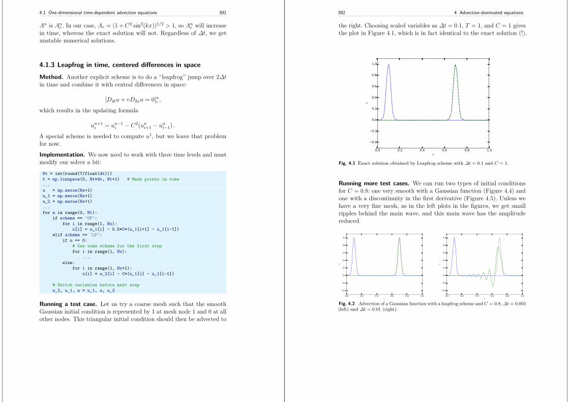
4.1 One-dimensional time-dependent advection equations 391
An is Anr . In our case, Ar = (1 +C2 sin2(kx))1/2 > 1, so Anr will increasein time, whereas the exact solution will not. Regardless of ∆t, we getunstable numerical solutions.
4.1.3 Leapfrog in time, centered differences in space
Method. Another explicit scheme is to do a “leapfrog” jump over 2∆tin time and combine it with central differences in space:
[D2tu+ vD2xu = 0]ni ,
which results in the updating formula
un+1i = un−1
i − C2(uni+1 − uni−1) .
A special scheme is needed to compute u1, but we leave that problemfor now.
Implementation. We now need to work with three time levels and mustmodify our solver a bit:
Nt = int(round(T/float(dt)))t = np.linspace(0, Nt*dt, Nt+1) # Mesh points in time...u = np.zeros(Nx+1)u_1 = np.zeros(Nx+1)u_2 = np.zeros(Nx+1)...for n in range(0, Nt):
if scheme == ’UP’:for i in range(1, Nx):
u[i] = u_1[i] - 0.5*C*(u_1[i+1] - u_1[i-1])elif scheme == ’LF’:
if n == 0:# Use some scheme for the first stepfor i in range(1, Nx):
...else:
for i in range(1, Nx+1):u[i] = u_2[i] - C*(u_1[i] - u_1[i-1])
# Switch variables before next stepu_2, u_1, u = u_1, u, u_2
Running a test case. Let us try a coarse mesh such that the smoothGaussian initial condition is represented by 1 at mesh node 1 and 0 at allother nodes. This triangular initial condition should then be advected to
392 4 Advection-dominated equations
the right. Choosing scaled variables as ∆t = 0.1, T = 1, and C = 1 givesthe plot in Figure 4.1, which is in fact identical to the exact solution (!).
0.0 0.2 0.4 0.6 0.8 1.0x
0.4
0.2
0.0
0.2
0.4
0.6
0.8
1.0
u
Fig. 4.1 Exact solution obtained by Leapfrog scheme with ∆t = 0.1 and C = 1.
Running more test cases. We can run two types of initial conditionsfor C = 0.8: one very smooth with a Gaussian function (Figure 4.4) andone with a discontinuity in the first derivative (Figure 4.5). Unless wehave a very fine mesh, as in the left plots in the figures, we get smallripples behind the main wave, and this main wave has the amplitudereduced.
0.0 0.2 0.4 0.6 0.8 1.0x
0.4
0.2
0.0
0.2
0.4
0.6
0.8
1.0
u
0.0 0.2 0.4 0.6 0.8 1.0x
0.4
0.2
0.0
0.2
0.4
0.6
0.8
1.0
u
Fig. 4.2 Advection of a Gaussian function with a leapfrog scheme and C = 0.8,∆t = 0.001(left) and ∆t = 0.01 (right).
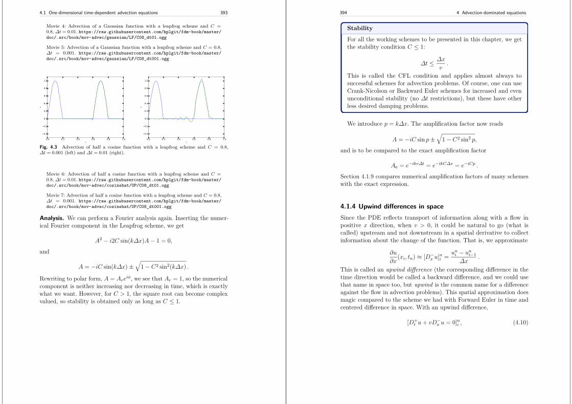
4.1 One-dimensional time-dependent advection equations 393
Movie 4: Advection of a Gaussian function with a leapfrog scheme and C =0.8, ∆t = 0.01. https://raw.githubusercontent.com/hplgit/fdm-book/master/doc/.src/book/mov-advec/gaussian/LF/C08_dt01.ogg
Movie 5: Advection of a Gaussian function with a leapfrog scheme and C = 0.8,∆t = 0.001. https://raw.githubusercontent.com/hplgit/fdm-book/master/doc/.src/book/mov-advec/gaussian/LF/C08_dt001.ogg
0.0 0.2 0.4 0.6 0.8 1.0x
0.4
0.2
0.0
0.2
0.4
0.6
0.8
1.0
u
0.0 0.2 0.4 0.6 0.8 1.0x
0.4
0.2
0.0
0.2
0.4
0.6
0.8
1.0
u
Fig. 4.3 Advection of half a cosine function with a leapfrog scheme and C = 0.8,∆t = 0.001 (left) and ∆t = 0.01 (right).
Movie 6: Advection of half a cosine function with a leapfrog scheme and C =0.8, ∆t = 0.01. https://raw.githubusercontent.com/hplgit/fdm-book/master/doc/.src/book/mov-advec/cosinehat/UP/C08_dt01.ogg
Movie 7: Advection of half a cosine function with a leapfrog scheme and C = 0.8,∆t = 0.001. https://raw.githubusercontent.com/hplgit/fdm-book/master/doc/.src/book/mov-advec/cosinehat/UP/C08_dt001.ogg
Analysis. We can perform a Fourier analysis again. Inserting the numer-ical Fourier component in the Leapfrog scheme, we get
A2 − i2C sin(k∆x)A− 1 = 0,
and
A = −iC sin(k∆x)±√
1− C2 sin2(k∆x) .
Rewriting to polar form, A = Areiφ, we see that Ar = 1, so the numerical
component is neither increasing nor decreasing in time, which is exactlywhat we want. However, for C > 1, the square root can become complexvalued, so stability is obtained only as long as C ≤ 1.
394 4 Advection-dominated equations
Stability
For all the working schemes to be presented in this chapter, we getthe stability condition C ≤ 1:
∆t ≤ ∆x
v.
This is called the CFL condition and applies almost always tosuccessful schemes for advection problems. Of course, one can useCrank-Nicolson or Backward Euler schemes for increased and evenunconditional stability (no ∆t restrictions), but these have otherless desired damping problems.
We introduce p = k∆x. The amplification factor now reads
A = −iC sin p±√
1− C2 sin2 p,
and is to be compared to the exact amplification factor
Ae = e−ikv∆t = e−ikC∆x = e−iCp .
Section 4.1.9 compares numerical amplification factors of many schemeswith the exact expression.
4.1.4 Upwind differences in spaceSince the PDE reflects transport of information along with a flow inpositive x direction, when v > 0, it could be natural to go (what iscalled) upstream and not downstream in a spatial derivative to collectinformation about the change of the function. That is, we approximate
∂u
∂x(xi, tn) ≈ [D−x u]ni = uni − uni−1
∆x.
This is called an upwind difference (the corresponding difference in thetime direction would be called a backward difference, and we could usethat name in space too, but upwind is the common name for a differenceagainst the flow in advection problems). This spatial approximation doesmagic compared to the scheme we had with Forward Euler in time andcentered difference in space. With an upwind difference,
[D+t u+ vD−x u = 0]ni , (4.10)
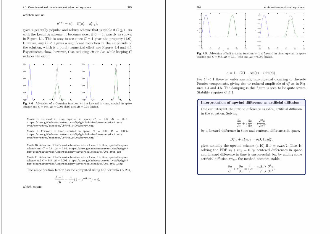
4.1 One-dimensional time-dependent advection equations 395
written out as
un+1 = uni − C(uni − uni−1),
gives a generally popular and robust scheme that is stable if C ≤ 1. Aswith the Leapfrog scheme, it becomes exact if C = 1, exactly as shownin Figure 4.1. This is easy to see since C = 1 gives the property (4.6).However, any C < 1 gives a significant reduction in the amplitude ofthe solution, which is a purely numerical effect, see Figures 4.4 and 4.5.Experiments show, however, that reducing ∆t or ∆x, while keeping Creduces the error.
0.0 0.2 0.4 0.6 0.8 1.00.0
0.2
0.4
0.6
0.8
1.0
0.0 0.2 0.4 0.6 0.8 1.00.0
0.2
0.4
0.6
0.8
1.0
Fig. 4.4 Advection of a Gaussian function with a forward in time, upwind in spacescheme and C = 0.8, ∆t = 0.001 (left) and ∆t = 0.01 (right).
Movie 8: Forward in time, upwind in space, C = 0.8, ∆t = 0.01.https://raw.githubusercontent.com/hplgit/fdm-book/master/doc/.src/book/mov-advec/gaussian/UP/C08_dt001/movie.ogg
Movie 9: Forward in time, upwind in space, C = 0.8, ∆t = 0.005.https://raw.githubusercontent.com/hplgit/fdm-book/master/doc/.src/book/mov-advec/gaussian/UP/C08_dt001/movie.ogg
Movie 10: Advection of half a cosine function with a forward in time, upwind in spacescheme and C = 0.8, ∆t = 0.01. https://raw.githubusercontent.com/hplgit/fdm-book/master/doc/.src/book/mov-advec/cosinehat/UP/C08_dt01.ogg
Movie 11: Advection of half a cosine function with a forward in time, upwind in spacescheme and C = 0.8, ∆t = 0.001. https://raw.githubusercontent.com/hplgit/fdm-book/master/doc/.src/book/mov-advec/cosinehat/UP/C08_dt001.ogg
The amplification factor can be computed using the formula (A.23),
A− 1∆t
+ v
∆x(1− e−ik∆x) = 0,
which means
396 4 Advection-dominated equations
0.0 0.2 0.4 0.6 0.8 1.0x
0.4
0.2
0.0
0.2
0.4
0.6
0.8
1.0
u
0.0 0.2 0.4 0.6 0.8 1.0x
0.4
0.2
0.0
0.2
0.4
0.6
0.8
1.0
u
Fig. 4.5 Advection of half a cosine function with a forward in time, upwind in spacescheme and C = 0.8, ∆t = 0.01 (left) and ∆t = 0.001 (right).
A = 1− C(1− cos(p)− i sin(p)) .
For C < 1 there is, unfortunately, non-physical damping of discreteFourier components, giving rise to reduced amplitude of uni as in Fig-ures 4.4 and 4.5. The damping is this figure is seen to be quite severe.Stability requires C ≤ 1.
Interpretation of upwind difference as artificial diffusion
One can interpret the upwind difference as extra, artificial diffusionin the equation. Solving
∂u
∂t+ v
∂u
∂x= ν
∂2u
∂x2 ,
by a forward difference in time and centered differences in space,
D+t u+ vD2xu = νDxDxu]ni ,
gives actually the upwind scheme (4.10) if ν = v∆x/2. That is,solving the PDE ut + vux = 0 by centered differences in spaceand forward difference in time is unsuccessful, but by adding someartificial diffusion νuxx, the method becomes stable:
∂u
∂t+ v
∂u
∂x=(α + v∆x
2
)∂2u
∂x2 .
4.1 One-dimensional time-dependent advection equations 397
4.1.5 Periodic boundary conditions
So far, we have given the value on the left boundary, un0 , and used thescheme to propagate the solution signal through the domain. Often, wewant to follow such signals for long time series, and periodic boundaryconditions are then relevant since they enable a signal that leaves theright boundary to immediately enter the left boundary and propagatethrough the domain again.
The periodic boundary condition is
u(0, t) = u(L, t), un0 = unNx .
It means that we in the first equation, involving un0 , insert unNx , and thatwe in the last equation, involving un+1
Nxinsert un+1
0 . Normally, we cando this in the simple way that u_1[0] is updated as u_1[Nx] at thebeginning of a new time level.
In some schemes we may need unNx+1 and un−1. Periodicity then meansthat these values are equal to un1 and unNx−1, respectively. For the upwindscheme it is sufficient to set u_1[0]=u_1[Nx] at a new time level beforecomputing u[1], which ensures that u[1] becomes right and at the nexttime level u[0] at the current time level is correctly updated. For theLeapfrog scheme we must update u[0] and u[Nx] using the scheme:
if periodic_bc:i = 0u[i] = u_2[i] - C*(u_1[i+1] - u_1[Nx-1])
for i in range(1, Nx):u[i] = u_2[i] - C*(u_1[i+1] - u_1[i-1])
if periodic_bc:u[Nx] = u[0]
4.1.6 Implementation
Test condition. Analytically, we can show that the integral in spaceunder the u(x, t) curve is constant:
398 4 Advection-dominated equations
∫ L
0
(∂u
∂t+ v
∂u
∂x
)dx = 0
∂
∂t
∫ L
0udx = −
∫ L
0v∂u
∂xdx
∂u
∂t
∫ L
0udx = [vu]L0 = 0
as long as u(0) = u(L) = 0. We can therefore use the property∫ L
0u(x, t)dx = const
as a partial verification during the simulation. Now, any numerical methodwith C 6= 1 will deviate from the constant, expected value, so the integralis a measure of the error in the scheme. The integral can be computedby the Trapezoidal integration rule
dx*(0.5*u[0] + 0.5*u[Nx] + np.sum(u[1:-1]))
if u is an array holding the solution.
The code. An appropriate solver function for multiple schemes maygo as shown below.
def solver(I, U0, v, L, dt, C, T, user_action=None,scheme=’FE’, periodic_bc=True):
Nt = int(round(T/float(dt)))t = np.linspace(0, Nt*dt, Nt+1) # Mesh points in timedx = v*dt/CNx = int(round(L/dx))x = np.linspace(0, L, Nx+1) # Mesh points in space# Make sure dx and dt are compatible with x and tdx = x[1] - x[0]dt = t[1] - t[0]C = v*dt/dxprint ’dt=%g, dx=%g, Nx=%d, C=%g’ % (dt, dx, Nx, C)
u = np.zeros(Nx+1)u_n = np.zeros(Nx+1)u_nm1 = np.zeros(Nx+1)integral = np.zeros(Nt+1)
# Set initial condition u(x,0) = I(x)for i in range(0, Nx+1):
u_n[i] = I(x[i])
# Insert boundary conditionu[0] = U0
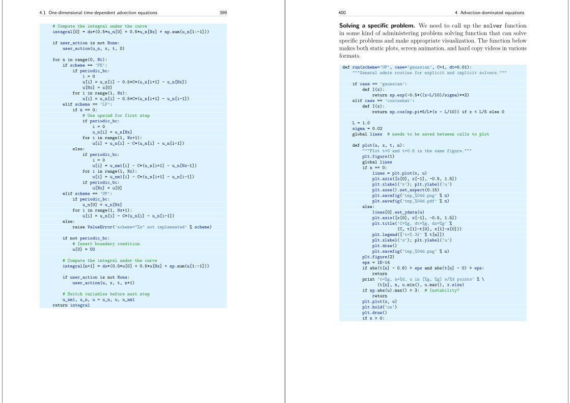
4.1 One-dimensional time-dependent advection equations 399
# Compute the integral under the curveintegral[0] = dx*(0.5*u_n[0] + 0.5*u_n[Nx] + np.sum(u_n[1:-1]))
if user_action is not None:user_action(u_n, x, t, 0)
for n in range(0, Nt):if scheme == ’FE’:
if periodic_bc:i = 0u[i] = u_n[i] - 0.5*C*(u_n[i+1] - u_n[Nx])u[Nx] = u[0]
for i in range(1, Nx):u[i] = u_n[i] - 0.5*C*(u_n[i+1] - u_n[i-1])
elif scheme == ’LF’:if n == 0:
# Use upwind for first stepif periodic_bc:
i = 0u_n[i] = u_n[Nx]
for i in range(1, Nx+1):u[i] = u_n[i] - C*(u_n[i] - u_n[i-1])
else:if periodic_bc:
i = 0u[i] = u_nm1[i] - C*(u_n[i+1] - u_n[Nx-1])
for i in range(1, Nx):u[i] = u_nm1[i] - C*(u_n[i+1] - u_n[i-1])
if periodic_bc:u[Nx] = u[0]
elif scheme == ’UP’:if periodic_bc:
u_n[0] = u_n[Nx]for i in range(1, Nx+1):
u[i] = u_n[i] - C*(u_n[i] - u_n[i-1])else:
raise ValueError(’scheme="%s" not implemented’ % scheme)
if not periodic_bc:# Insert boundary conditionu[0] = U0
# Compute the integral under the curveintegral[n+1] = dx*(0.5*u[0] + 0.5*u[Nx] + np.sum(u[1:-1]))
if user_action is not None:user_action(u, x, t, n+1)
# Switch variables before next stepu_nm1, u_n, u = u_n, u, u_nm1
return integral
400 4 Advection-dominated equations
Solving a specific problem. We need to call up the solver functionin some kind of administering problem solving function that can solvespecific problems and make appropriate visualization. The function belowmakes both static plots, screen animation, and hard copy videos in variousformats.
def run(scheme=’UP’, case=’gaussian’, C=1, dt=0.01):"""General admin routine for explicit and implicit solvers."""
if case == ’gaussian’:def I(x):
return np.exp(-0.5*((x-L/10)/sigma)**2)elif case == ’cosinehat’:
def I(x):return np.cos(np.pi*5/L*(x - L/10)) if x < L/5 else 0
L = 1.0sigma = 0.02global lines # needs to be saved between calls to plot
def plot(u, x, t, n):"""Plot t=0 and t=0.6 in the same figure."""plt.figure(1)global linesif n == 0:
lines = plt.plot(x, u)plt.axis([x[0], x[-1], -0.5, 1.5])plt.xlabel(’x’); plt.ylabel(’u’)plt.axes().set_aspect(0.15)plt.savefig(’tmp_%04d.png’ % n)plt.savefig(’tmp_%04d.pdf’ % n)
else:lines[0].set_ydata(u)plt.axis([x[0], x[-1], -0.5, 1.5])plt.title(’C=%g, dt=%g, dx=%g’ %
(C, t[1]-t[0], x[1]-x[0]))plt.legend([’t=%.3f’ % t[n]])plt.xlabel(’x’); plt.ylabel(’u’)plt.draw()plt.savefig(’tmp_%04d.png’ % n)
plt.figure(2)eps = 1E-14if abs(t[n] - 0.6) > eps and abs(t[n] - 0) > eps:
returnprint ’t=%g, n=%d, u in [%g, %g] w/%d points’ % \
(t[n], n, u.min(), u.max(), x.size)if np.abs(u).max() > 3: # Instability?
returnplt.plot(x, u)plt.hold(’on’)plt.draw()if n > 0:
4.1 One-dimensional time-dependent advection equations 401
y = [I(x_-v*t[n]) for x_ in x]plt.plot(x, y, ’k--’)if abs(t[n] - 0.6) < eps:
filename = (’tmp_%s_dt%s_C%s’ % \(scheme, t[1]-t[0], C)).replace(’.’, ’’)
np.savez(filename, x=x, u=u, u_e=y)
plt.ion()U0 = 0T = 0.7v = 1# Define video formats and librariescodecs = dict(flv=’flv’, mp4=’libx264’, webm=’libvpx’,
ogg=’libtheora’)# Remove video filesimport glob, osfor name in glob.glob(’tmp_*.png’):
os.remove(name)for ext in codecs:
name = ’movie.%s’ % extif os.path.isfile(name):
os.remove(name)
integral = solver(I=I, U0=U0, v=v, L=L, dt=dt, C=C, T=T,scheme=scheme, user_action=plot)
# Finish up figure(2)plt.figure(2)plt.axis([0, L, -0.5, 1.1])plt.xlabel(’$x$’); plt.ylabel(’$u$’)plt.savefig(’tmp1.png’); plt.savefig(’tmp1.pdf’)plt.show()# Make videos from figure(1) animation filesfor codec in codecs:
cmd = ’ffmpeg -i tmp_%%04d.png -r 25 -vcodec %s movie.%s’ % \(codecs[codec], codec)
os.system(cmd)print ’Integral of u:’, integral.max(), integral.min()
The complete code is found in the file advec1D.py.
4.1.7 A Crank-Nicolson discretization in time and centereddifferences in space
Another obvious candidate for time discretization is the Crank-Nicolsonmethod combined with centered differences in space:
[Dtu]ni + v12([D2xu]n+1
i + [D2xu]ni ) = 0 .
It can be nice to include the Backward Euler scheme too, via the θ-rule,
402 4 Advection-dominated equations
[Dtu]ni + vθ[D2xu]n+1i + v(1− θ)[D2xu]ni = 0 .
This gives rise to an implicit scheme,
un+1i + θ
2C(un+1i+1 − un+1
i−1 ) = uni −1− θ
2 C(uni+1 − uni−1)
for i = 1, . . . , Nx−1. At the boundaries we set u = 0 and simulate just tothe point of time when the signal hits the boundary (and gets reflected).
un+10 = un+1
Nx= 0 .
The elements on the diagonal in the matrix become:
Ai,i = 1, i = 0, . . . , Nx .
On the subdiagonal and superdiagonal we have
Ai−1,i = −θ2C, Ai+1,i = θ
2C, i = 1, . . . , Nx − 1,
with A0,1 = 0 and ANx−1,Nx = 0 due to the known boundary conditions.And finally, the right-hand side becomes
b0 = unNx
bi = uni −1− θ
2 C(uni+1 − uni−1), i = 1, . . . , Nx − 1
bNx = un0
The dispersion relation follows from inserting uni = Aneikx and usingthe formula (A.25) for the spatial differences:
A = 1− (1− θ)iC sin p1 + θiC sin p .
Movie 12: Crank-Nicolson in time, centered in space, C = 0.8, ∆t = 0.005.https://raw.githubusercontent.com/hplgit/fdm-book/master/doc/.src/book/mov-advec/gaussian/CN/C08_dt0005/movie.ogg
Movie 13: Backward-Euler in time, centered in space, C = 0.8, ∆t = 0.005.https://raw.githubusercontent.com/hplgit/fdm-book/master/doc/.src/book/mov-advec/cosinehat/BE/C_08_dt005.ogg
Figure 4.6 depicts a numerical solution for C = 0.8 and the Crank-Nicolson with severe oscillations behind the main wave. These oscillations
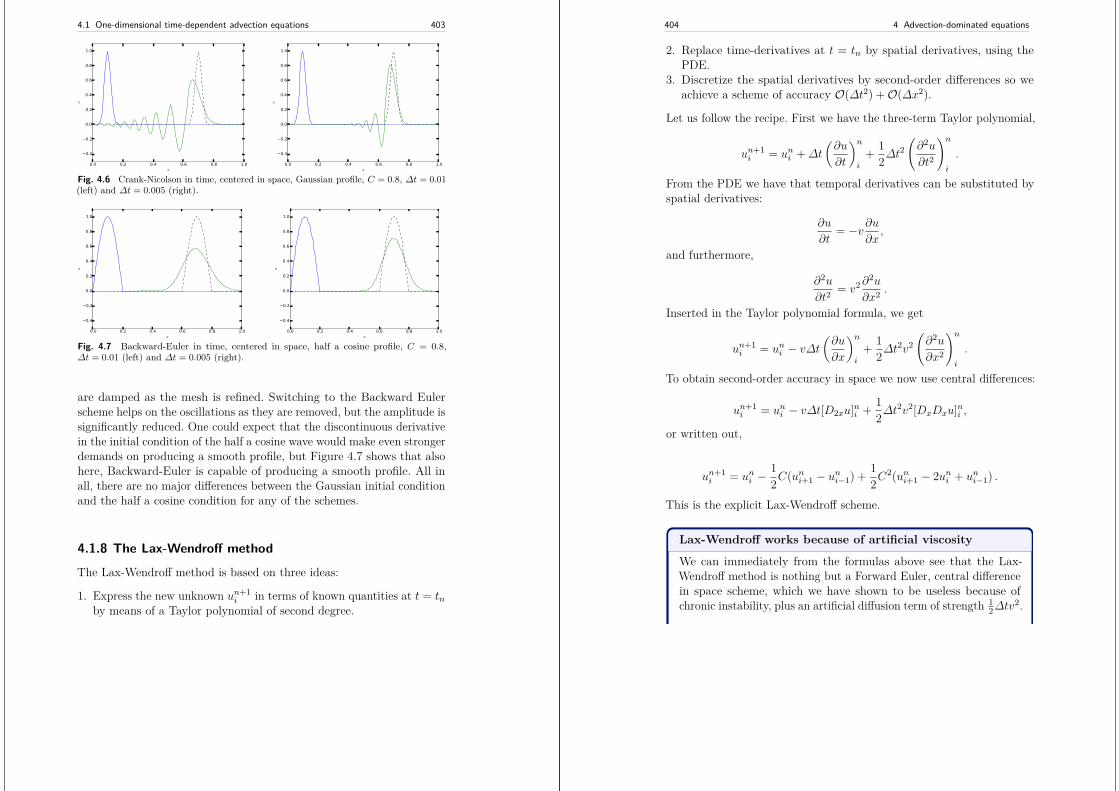
4.1 One-dimensional time-dependent advection equations 403
0.0 0.2 0.4 0.6 0.8 1.0x
0.4
0.2
0.0
0.2
0.4
0.6
0.8
1.0
u
0.0 0.2 0.4 0.6 0.8 1.0x
0.4
0.2
0.0
0.2
0.4
0.6
0.8
1.0
u
Fig. 4.6 Crank-Nicolson in time, centered in space, Gaussian profile, C = 0.8, ∆t = 0.01(left) and ∆t = 0.005 (right).
0.0 0.2 0.4 0.6 0.8 1.0x
0.4
0.2
0.0
0.2
0.4
0.6
0.8
1.0
u
0.0 0.2 0.4 0.6 0.8 1.0x
0.4
0.2
0.0
0.2
0.4
0.6
0.8
1.0
u
Fig. 4.7 Backward-Euler in time, centered in space, half a cosine profile, C = 0.8,∆t = 0.01 (left) and ∆t = 0.005 (right).
are damped as the mesh is refined. Switching to the Backward Eulerscheme helps on the oscillations as they are removed, but the amplitude issignificantly reduced. One could expect that the discontinuous derivativein the initial condition of the half a cosine wave would make even strongerdemands on producing a smooth profile, but Figure 4.7 shows that alsohere, Backward-Euler is capable of producing a smooth profile. All inall, there are no major differences between the Gaussian initial conditionand the half a cosine condition for any of the schemes.
4.1.8 The Lax-Wendroff method
The Lax-Wendroff method is based on three ideas:
1. Express the new unknown un+1i in terms of known quantities at t = tn
by means of a Taylor polynomial of second degree.
404 4 Advection-dominated equations
2. Replace time-derivatives at t = tn by spatial derivatives, using thePDE.
3. Discretize the spatial derivatives by second-order differences so weachieve a scheme of accuracy O(∆t2) +O(∆x2).
Let us follow the recipe. First we have the three-term Taylor polynomial,
un+1i = uni +∆t
(∂u
∂t
)n
i
+ 12∆t
2(∂2u
∂t2
)n
i
.
From the PDE we have that temporal derivatives can be substituted byspatial derivatives:
∂u
∂t= −v∂u
∂x,
and furthermore,
∂2u
∂t2= v2∂
2u
∂x2 .
Inserted in the Taylor polynomial formula, we get
un+1i = uni − v∆t
(∂u
∂x
)n
i
+ 12∆t
2v2(∂2u
∂x2
)n
i
.
To obtain second-order accuracy in space we now use central differences:
un+1i = uni − v∆t[D2xu]ni + 1
2∆t2v2[DxDxu]ni ,
or written out,
un+1i = uni −
12C(uni+1 − uni−1) + 1
2C2(uni+1 − 2uni + uni−1) .
This is the explicit Lax-Wendroff scheme.
Lax-Wendroff works because of artificial viscosity
We can immediately from the formulas above see that the Lax-Wendroff method is nothing but a Forward Euler, central differencein space scheme, which we have shown to be useless because ofchronic instability, plus an artificial diffusion term of strength 1
2∆tv2.
4.1 One-dimensional time-dependent advection equations 405
It means that we can take an unstable scheme and add somediffusion to stabilize it. This is a common trick to deal with advectionproblems. Sometimes, the real physical diffusion is not sufficientlylarge to make schemes stable, so then we also add artificial diffusion.
From an analysis similar to the ones carried out above, we get anamplification factor for the Lax-Wendroff method that equals
A = 1− iC sin p− 2C2 sin2(p/2) .
This means that |A| = 1 and also that we have an exact solution ofC = 1!
4.1.9 Analysis of dispersion relations
We have developed expressions for A(C, p) in the exact solution unq =Aneikq∆x of the discrete equations. These expressions are valuablefor investigating the quality of the numerical solutions, see the filedispersion_analysis.py. Note that the Fourier component that solvesthe original PDE problem has no damping and moves with constantvelocity v. There are two basic errors in the numerical Fourier component:there may be damping and the wave velocity may depend on C andp = k∆x.
The shortest wavelength that can be represented is λ = 2∆x. Thecorresponding k is k = 2π/λ = π/∆x, so p = k∆x ∈ (0, π].
Given a complex A as a function of C and p, how can we visualize it?The two key ingredients in A is the magnitude, reflecting damping orgrowth of the wave, and the angle, closely related to the velocity of thewave. The Fourier component
Dneik(x−ct)
has damping D and wave velocity c. Let us express our A in polarform, A = Are
iφ, and insert this expression in our discrete componentunq = Aneikq∆x = Aneikx:
unq = Anr eiφneikx = Anr e
i(kx−nφ) = Anr ei(k(x−ct)),
for
406 4 Advection-dominated equations
c = φ
k∆t.
Now,
k∆t = Ck∆x
v= Cp
v,
so
c = φv
Cp.
An appropriate dimensionless quantity to plot is the scaled wave velocityc/v:
c
v= φ
Cp.
Figures 4.8–4.13 contain dispersion curves, velocity and damping,for various values of C. The horizontal axis shows the dimensionlessfrequency p of the wave, while the figures to the left illustrate the errorin wave velocity c/v (should ideally be 1 for all p), and the figures to theright display the absolute value (magnitude) of the damping factor Ar.The curves are labeled according to the table below.
Label MethodFE Forward Euler in time, centered difference in spaceLF Leapfrog in time, centered difference in spaceUP Forward Euler in time, upwind difference in spaceCN Crank-Nicolson in time, centered difference in spaceLW Lax-Wendroff’s methodBE Backward Euler in time, centered difference in space
0.0 0.5 1.0 1.5 2.0 2.5 3.0 3.5p
1.2
1.0
0.8
0.6
0.4
0.2
0.0
0.2
c/v
C=1
LWUPLF
0.0 0.5 1.0 1.5 2.0 2.5 3.0 3.5p
0.94
0.96
0.98
1.00
1.02
1.04
1.06
Ar
C=1
LWUPLF
Fig. 4.8 Dispersion relations for C = 1.
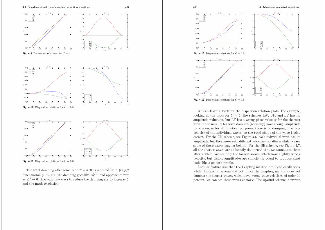
4.1 One-dimensional time-dependent advection equations 407
0.0 0.5 1.0 1.5 2.0 2.5 3.0 3.5p
1.0
0.8
0.6
0.4
0.2
0.0
c/v
C=1
CNBEFE
0.0 0.5 1.0 1.5 2.0 2.5 3.0 3.5p
0.7
0.8
0.9
1.0
1.1
1.2
1.3
1.4
1.5
Ar
C=1
CNBEFE
Fig. 4.9 Dispersion relations for C = 1.
0.0 0.5 1.0 1.5 2.0 2.5 3.0 3.5p
1.4
1.2
1.0
0.8
0.6
0.4
0.2
0.0
0.2
c/v
C=0.8
LWUPLF
0.0 0.5 1.0 1.5 2.0 2.5 3.0 3.5p
0.2
0.3
0.4
0.5
0.6
0.7
0.8
0.9
1.0
Ar
C=0.8
LWUPLF
Fig. 4.10 Dispersion relations for C = 0.8.
0.0 0.5 1.0 1.5 2.0 2.5 3.0 3.5p
1.0
0.8
0.6
0.4
0.2
0.0
c/v
C=0.8
CNBEFE
0.0 0.5 1.0 1.5 2.0 2.5 3.0 3.5p
0.7
0.8
0.9
1.0
1.1
1.2
1.3
Ar
C=0.8
CNBEFE
Fig. 4.11 Dispersion relations for C = 0.8.
The total damping after some time T = n∆t is reflected by Ar(C, p)n.Since normally Ar < 1, the damping goes like A1/∆t
r and approaches zeroas ∆t→ 0. The only two ways to reduce the damping are to increase Cand the mesh resolution.
408 4 Advection-dominated equations
0.0 0.5 1.0 1.5 2.0 2.5 3.0 3.5p
1.2
1.0
0.8
0.6
0.4
0.2
0.0
0.2
c/v
C=0.5
LWUPLF
0.0 0.5 1.0 1.5 2.0 2.5 3.0 3.5p
0.0
0.2
0.4
0.6
0.8
1.0
Ar
C=0.5
LWUPLF
Fig. 4.12 Dispersion relations for C = 0.5.
0.0 0.5 1.0 1.5 2.0 2.5 3.0 3.5p
1.0
0.8
0.6
0.4
0.2
0.0
c/v
C=0.5
CNBEFE
0.0 0.5 1.0 1.5 2.0 2.5 3.0 3.5p
0.85
0.90
0.95
1.00
1.05
1.10
1.15
Ar
C=0.5
CNBEFE
Fig. 4.13 Dispersion relations for C = 0.5.
We can learn a lot from the dispersion relation plots. For example,looking at the plots for C = 1, the schemes LW, UP, and LF has noamplitude reduction, but LF has a wrong phase velocity for the shortestwave in the mesh. This wave does not (normally) have enough amplitudeto be seen, so for all practical purposes, there is no damping or wrongvelocity of the individual waves, so the total shape of the wave is alsocorrect. For the CN scheme, see Figure 4.6, each individual wave has itsamplitude, but they move with different velocities, so after a while, we seesome of these waves lagging behind. For the BE scheme, see Figure 4.7,all the shorter waves are so heavily dampened that we cannot see themafter a while. We see only the longest waves, which have slightly wrongvelocity, but visible amplitudes are sufficiently equal to produce whatlooks like a smooth profile.
Another feature was that the Leapfrog method produced oscillations,while the upwind scheme did not. Since the Leapfrog method does notdampen the shorter waves, which have wrong wave velocities of order 10percent, we can see these waves as noise. The upwind scheme, however,
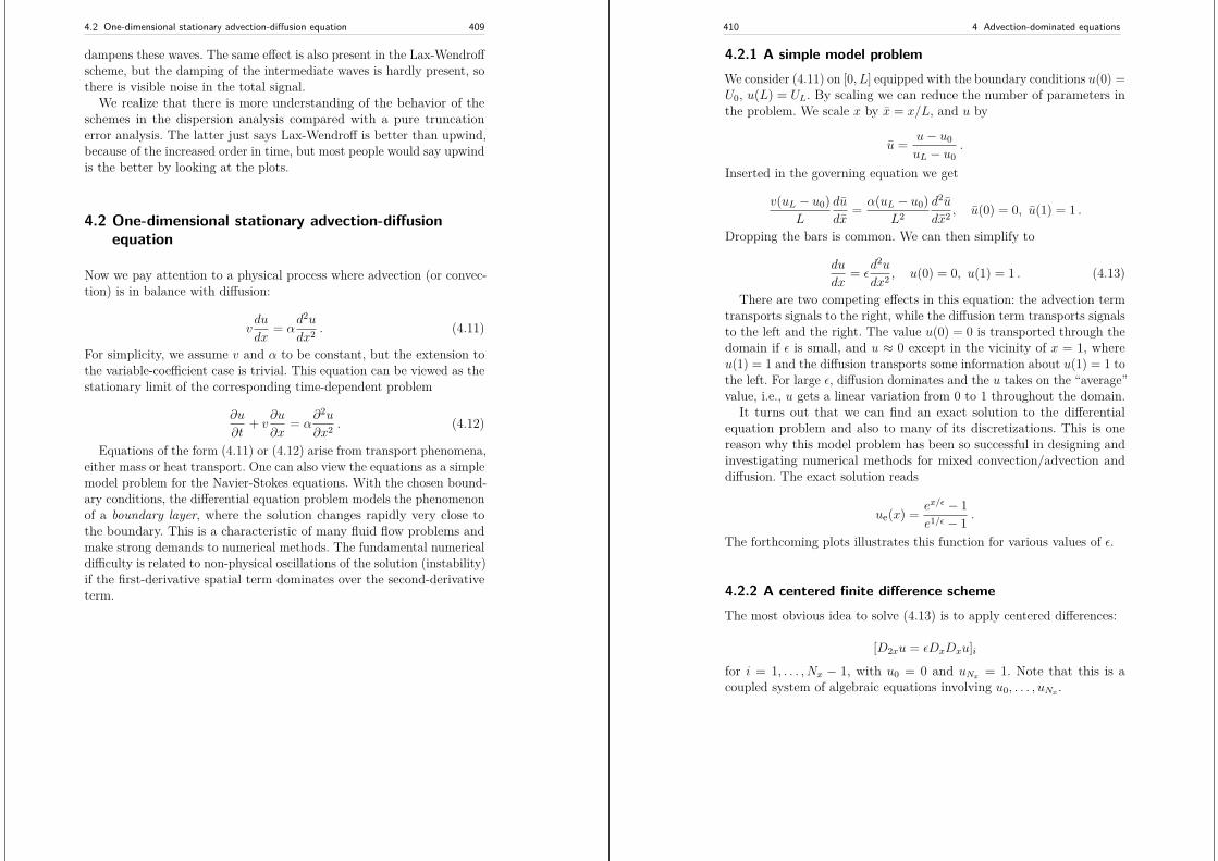
4.2 One-dimensional stationary advection-diffusion equation 409
dampens these waves. The same effect is also present in the Lax-Wendroffscheme, but the damping of the intermediate waves is hardly present, sothere is visible noise in the total signal.
We realize that there is more understanding of the behavior of theschemes in the dispersion analysis compared with a pure truncationerror analysis. The latter just says Lax-Wendroff is better than upwind,because of the increased order in time, but most people would say upwindis the better by looking at the plots.
4.2 One-dimensional stationary advection-diffusionequation
Now we pay attention to a physical process where advection (or convec-tion) is in balance with diffusion:
vdu
dx= α
d2u
dx2 . (4.11)
For simplicity, we assume v and α to be constant, but the extension tothe variable-coefficient case is trivial. This equation can be viewed as thestationary limit of the corresponding time-dependent problem
∂u
∂t+ v
∂u
∂x= α
∂2u
∂x2 . (4.12)
Equations of the form (4.11) or (4.12) arise from transport phenomena,either mass or heat transport. One can also view the equations as a simplemodel problem for the Navier-Stokes equations. With the chosen bound-ary conditions, the differential equation problem models the phenomenonof a boundary layer, where the solution changes rapidly very close tothe boundary. This is a characteristic of many fluid flow problems andmake strong demands to numerical methods. The fundamental numericaldifficulty is related to non-physical oscillations of the solution (instability)if the first-derivative spatial term dominates over the second-derivativeterm.
410 4 Advection-dominated equations
4.2.1 A simple model problemWe consider (4.11) on [0, L] equipped with the boundary conditions u(0) =U0, u(L) = UL. By scaling we can reduce the number of parameters inthe problem. We scale x by x = x/L, and u by
u = u− u0uL − u0
.
Inserted in the governing equation we get
v(uL − u0)L
du
dx= α(uL − u0)
L2d2u
dx2 , u(0) = 0, u(1) = 1 .
Dropping the bars is common. We can then simplify to
du
dx= ε
d2u
dx2 , u(0) = 0, u(1) = 1 . (4.13)
There are two competing effects in this equation: the advection termtransports signals to the right, while the diffusion term transports signalsto the left and the right. The value u(0) = 0 is transported through thedomain if ε is small, and u ≈ 0 except in the vicinity of x = 1, whereu(1) = 1 and the diffusion transports some information about u(1) = 1 tothe left. For large ε, diffusion dominates and the u takes on the “average”value, i.e., u gets a linear variation from 0 to 1 throughout the domain.
It turns out that we can find an exact solution to the differentialequation problem and also to many of its discretizations. This is onereason why this model problem has been so successful in designing andinvestigating numerical methods for mixed convection/advection anddiffusion. The exact solution reads
ue(x) = ex/ε − 1e1/ε − 1 .
The forthcoming plots illustrates this function for various values of ε.
4.2.2 A centered finite difference schemeThe most obvious idea to solve (4.13) is to apply centered differences:
[D2xu = εDxDxu]ifor i = 1, . . . , Nx − 1, with u0 = 0 and uNx = 1. Note that this is acoupled system of algebraic equations involving u0, . . . , uNx .
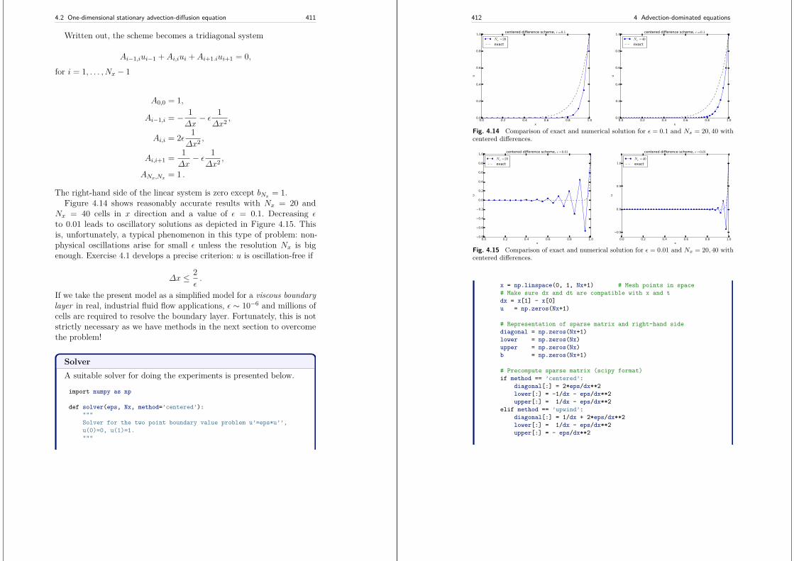
4.2 One-dimensional stationary advection-diffusion equation 411
Written out, the scheme becomes a tridiagonal system
Ai−1,iui−1 + Ai,iui + Ai+1.iui+1 = 0,
for i = 1, . . . , Nx − 1
A0,0 = 1,
Ai−1,i = − 1∆x− ε 1
∆x2 ,
Ai,i = 2ε 1∆x2 ,
Ai,i+1 = 1∆x− ε 1
∆x2 ,
ANx,Nx = 1 .
The right-hand side of the linear system is zero except bNx = 1.Figure 4.14 shows reasonably accurate results with Nx = 20 and
Nx = 40 cells in x direction and a value of ε = 0.1. Decreasing εto 0.01 leads to oscillatory solutions as depicted in Figure 4.15. Thisis, unfortunately, a typical phenomenon in this type of problem: non-physical oscillations arise for small ε unless the resolution Nx is bigenough. Exercise 4.1 develops a precise criterion: u is oscillation-free if
∆x ≤ 2ε.
If we take the present model as a simplified model for a viscous boundarylayer in real, industrial fluid flow applications, ε ∼ 10−6 and millions ofcells are required to resolve the boundary layer. Fortunately, this is notstrictly necessary as we have methods in the next section to overcomethe problem!
SolverA suitable solver for doing the experiments is presented below.
import numpy as np
def solver(eps, Nx, method=’centered’):"""Solver for the two point boundary value problem u’=eps*u’’,u(0)=0, u(1)=1."""
412 4 Advection-dominated equations
0.0 0.2 0.4 0.6 0.8 1.0x
0.0
0.2
0.4
0.6
0.8
1.0
u
centered difference scheme, ε=0.1
Nx =20
exact
0.0 0.2 0.4 0.6 0.8 1.0x
0.0
0.2
0.4
0.6
0.8
1.0
u
centered difference scheme, ε=0.1
Nx =40
exact
Fig. 4.14 Comparison of exact and numerical solution for ε = 0.1 and Nx = 20, 40 withcentered differences.
0.0 0.2 0.4 0.6 0.8 1.0x
0.8
0.6
0.4
0.2
0.0
0.2
0.4
0.6
0.8
1.0
u
centered difference scheme, ε=0.01
Nx =20
exact
0.0 0.2 0.4 0.6 0.8 1.0x
0.5
0.0
0.5
1.0
u
centered difference scheme, ε=0.01
Nx =40
exact
Fig. 4.15 Comparison of exact and numerical solution for ε = 0.01 and Nx = 20, 40 withcentered differences.
x = np.linspace(0, 1, Nx+1) # Mesh points in space# Make sure dx and dt are compatible with x and tdx = x[1] - x[0]u = np.zeros(Nx+1)
# Representation of sparse matrix and right-hand sidediagonal = np.zeros(Nx+1)lower = np.zeros(Nx)upper = np.zeros(Nx)b = np.zeros(Nx+1)
# Precompute sparse matrix (scipy format)if method == ’centered’:
diagonal[:] = 2*eps/dx**2lower[:] = -1/dx - eps/dx**2upper[:] = 1/dx - eps/dx**2
elif method == ’upwind’:diagonal[:] = 1/dx + 2*eps/dx**2lower[:] = 1/dx - eps/dx**2upper[:] = - eps/dx**2
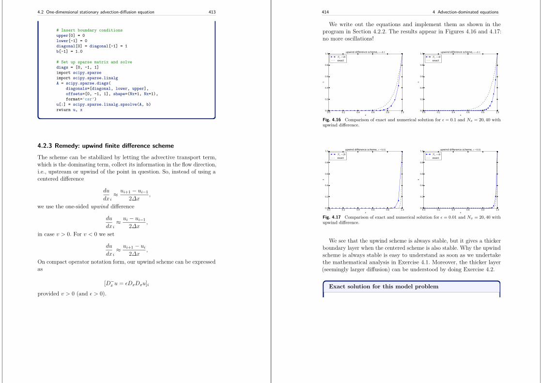
4.2 One-dimensional stationary advection-diffusion equation 413
# Insert boundary conditionsupper[0] = 0lower[-1] = 0diagonal[0] = diagonal[-1] = 1b[-1] = 1.0
# Set up sparse matrix and solvediags = [0, -1, 1]import scipy.sparseimport scipy.sparse.linalgA = scipy.sparse.diags(
diagonals=[diagonal, lower, upper],offsets=[0, -1, 1], shape=(Nx+1, Nx+1),format=’csr’)
u[:] = scipy.sparse.linalg.spsolve(A, b)return u, x
4.2.3 Remedy: upwind finite difference scheme
The scheme can be stabilized by letting the advective transport term,which is the dominating term, collect its information in the flow direction,i.e., upstream or upwind of the point in question. So, instead of using acentered difference
du
dx i≈ ui+1 − ui−1
2∆x ,
we use the one-sided upwind difference
du
dx i≈ ui − ui−1
2∆x ,
in case v > 0. For v < 0 we set
du
dx i≈ ui+1 − ui
2∆x ,
On compact operator notation form, our upwind scheme can be expressedas
[D−x u = εDxDxu]iprovided v > 0 (and ε > 0).
414 4 Advection-dominated equations
We write out the equations and implement them as shown in theprogram in Section 4.2.2. The results appear in Figures 4.16 and 4.17:no more oscillations!
0.0 0.2 0.4 0.6 0.8 1.0x
0.0
0.2
0.4
0.6
0.8
1.0
u
upwind difference scheme, ε=0.1
Nx =20
exact
0.0 0.2 0.4 0.6 0.8 1.0x
0.0
0.2
0.4
0.6
0.8
1.0
u
upwind difference scheme, ε=0.1
Nx =40
exact
Fig. 4.16 Comparison of exact and numerical solution for ε = 0.1 and Nx = 20, 40 withupwind difference.
0.0 0.2 0.4 0.6 0.8 1.0x
0.0
0.2
0.4
0.6
0.8
1.0
u
upwind difference scheme, ε=0.01
Nx =20
exact
0.0 0.2 0.4 0.6 0.8 1.0x
0.0
0.2
0.4
0.6
0.8
1.0
u
upwind difference scheme, ε=0.01
Nx =40
exact
Fig. 4.17 Comparison of exact and numerical solution for ε = 0.01 and Nx = 20, 40 withupwind difference.
We see that the upwind scheme is always stable, but it gives a thickerboundary layer when the centered scheme is also stable. Why the upwindscheme is always stable is easy to understand as soon as we undertakethe mathematical analysis in Exercise 4.1. Moreover, the thicker layer(seemingly larger diffusion) can be understood by doing Exercise 4.2.
Exact solution for this model problem
4.3 Time-dependent convection-diffusion equations 415
It turns out that one can introduce a linear combination of thecentered and upwind differences for the first-derivative term inthis model problem. One can then adjust the weight in the linearcombination so that the numerical solution becomes identical tothe analytical solution of the differential equation problem at anymesh point.
4.3 Time-dependent convection-diffusion equations
Now it is time to combine time-dependency, convection (advection) anddiffusion into one equation:
∂u
∂t+ v
∂u
∂x= α
∂2u
∂x2 . (4.14)
Analytical insight. The diffusion is now dominated by convection, awave, and diffusion, a loss of amplitude. One possible analytical solutionis a traveling Gaussian function
u(x, t) = B exp(−(x− vt
4at
)).
This function moves with velocity v > 0 to the right (v < 0 to the left)due to convection, but at the same time we have a damping e−16a2t2 fromdiffusion.
4.3.1 Forward in time, centered in space scheme
The Forward Euler for the diffusion equation is a successful scheme, but ithas a very strict stability condition. The similar Forward in time, centeredin space strategy always gives unstable solutions for the advection PDE.What happens when we have both diffusion and advection present atonce?
[Dtu+ vD2xu = αDxDxu+ f ]ni .
We expect that diffusion will stabilize the scheme, but that advectionwill destabilize it.
416 4 Advection-dominated equations
Another problem is non-physical oscillations, but not growing am-plitudes, due to centered differences in the advection term. There willhence be two types of instabilities to consider. Our analysis showed thatpure advection with centered differences in space needs some artificialdiffusion to become stable (and then it produces upwind differences forthe advection term). Adding more physical diffusion should further helpthe numerics to stabilize the non-physical oscillations.
The scheme is quickly implemented, but suffers from the need for smallspace and time steps, according to this reasoning. A better approach isto get rid of the non-physical oscillations in space by simply applying anupwind difference on the advection term.
4.3.2 Forward in time, upwind in space schemeA good approximation for the pure advection equation is to use upwinddiscretization of the advection term. We also know that centered dif-ferences are good for the diffusion term, so let us combine these twodiscretizations:
[Dtu+ vD−x u = αDxDxu+ f ]ni , (4.15)
for v > 0. Use vD+u if v < 0. In this case the physical diffusion andthe extra numerical diffusion v∆x/2 will stabilize the solution, but givean overall too large reduction in amplitude compared with the exactsolution.
We may also interpret the upwind difference as artificial numericaldiffusion and centered differences in space everywhere, so the scheme canbe expressed as
[Dtu+ vD−2xu = αv∆x
2 )DxDxu+ f ]ni . (4.16)
4.4 Two-dimensional advection-diffusion equations
4.5 Applications of advection equations
There are two major areas where advection and convection applicationsarise: transport of a substance and heat transport in a fluid. To derivethe models, we may look at the similar derivations of diffusion models
4.5 Applications of advection equations 417
in Section 3.8, but change the assumption from a solid to fluid medium.This gives rise to the extra advection or convection term v · ∇u. Webriefly show how this is done.
Normally, transport in a fluid is dominated by the fluid flow and notdiffusion, so we can neglect diffusion compared to advection or convection.The end result is anyway an equation of the form
∂u
∂t+ v · ∇u = 0 .
4.5.1 Transport of a substance
The diffusion of a substance in Section 3.8.1 takes place in a solid medium,but in a fluid we can have two transport mechanisms: one by diffusionand one by advection. The latter arises from the fact that the substanceparticles are moved with the fluid velocity v such that the effective fluxnow consists of two and not only one component as in (3.122):
q = −α∇c+ v .
Inserted in the equation ∇ · q = 0 we get the extra advection term∇· (v). Very often we deal with incompressible flows, ∇·v = 0 such thatthe advective term becomes v · ∇c. The mass transport equation for asubstance then reads
∂c
∂t+ v · ∇c = α∇2c . (4.17)
4.5.2 Transport of a heat
The derivation of the heat equation in Section 3.8.2 is limited to heattransport in solid bodies. If we turn the attention to heat transport influids, we get a material derivative of the internal energy in (3.124),
De
dt= −∇ · q,
and more terms if work by stresses is also included, where
De
dt= ∂e
∂t+ v · ∇e,
418 4 Advection-dominated equations
v being the velocity of the fluid. The convective term v ·∇e must thereforebe added to the governing equation, resulting typically in
%c
(∂T
∂t+ v · ∇T
)= ∇ · (k∇T ) + f, (4.18)
where f is some external heating inside the medium.
4.6 Exercises
Exercise 4.1: Analyze 1D stationary convection-diffusionproblem
Explain the observations in the numerical experiments from Sections 4.2.2and 4.2.3 by finding exact numerical solutions.
Hint. The difference equations allow solutions on the form Ai, where Ais an unknown constant and i is a mesh point counter. There are twosolutions for A, so the general solution is a linear combination of the two,where the constants in the linear combination are determined from theboundary conditions.Filename: twopt_BVP_analysis1.
Exercise 4.2: Interpret upwind difference as artificial diffusion
Consider an upwind, one-sided difference approximation to a term du/dxin a differential equation. Show that this formula can be expressed as a cen-tered difference plus an artificial diffusion term of strength proportional to∆x. This means that introducing an upwind difference also means intro-ducing extra diffusion of order O(∆x). Filename: twopt_BVP_analysis2.
Nonlinear problems 5
5.1 Introduction of basic concepts
5.1.1 Linear versus nonlinear equations
Algebraic equations. A linear, scalar, algebraic equation in x has theform
ax+ b = 0,
for arbitrary real constants a and b. The unknown is a number x. Allother algebraic equations, e.g., x2 +ax+ b = 0, are nonlinear. The typicalfeature in a nonlinear algebraic equation is that the unknown appears inproducts with itself, like x2 or ex = 1 + x+ 1
2x2 + 1
3!x3 + · · · .
We know how to solve a linear algebraic equation, x = −b/a, butthere are no general methods for finding the exact solutions of nonlinearalgebraic equations, except for very special cases (quadratic equationsconstitute a primary example). A nonlinear algebraic equation mayhave no solution, one solution, or many solutions. The tools for solvingnonlinear algebraic equations are iterative methods, where we construct aseries of linear equations, which we know how to solve, and hope that thesolutions of the linear equations converge to a solution of the nonlinearequation we want to solve. Typical methods for nonlinear algebraicequation equations are Newton’s method, the Bisection method, and theSecant method.
© 2016, Hans Petter Langtangen, Svein Linge. Released under CC Attribution 4.0 license
420 5 Nonlinear problems
Differential equations. The unknown in a differential equation is afunction and not a number. In a linear differential equation, all termsinvolving the unknown function are linear in the unknown function or itsderivatives. Linear here means that the unknown function, or a derivativeof it, is multiplied by a number or a known function. All other differentialequations are non-linear.
The easiest way to see if an equation is nonlinear, is to spot nonlinearterms where the unknown function or its derivatives are multiplied byeach other. For example, in
u′(t) = −a(t)u(t) + b(t),
the terms involving the unknown function u are linear: u′ contains thederivative of the unknown function multiplied by unity, and au containsthe unknown function multiplied by a known function. However,
u′(t) = u(t)(1− u(t)),
is nonlinear because of the term −u2 where the unknown function ismultiplied by itself. Also
∂u
∂t+ u
∂u
∂x= 0,
is nonlinear because of the term uux where the unknown function appearsin a product with its derivative. (Note here that we use different notationsfor derivatives: u′ or du/dt for a function u(t) of one variable, ∂u∂t or utfor a function of more than one variable.)
Another example of a nonlinear equation is
u′′ + sin(u) = 0,
because sin(u) contains products of u, which becomes clear if we expandthe function in a Taylor series:
sin(u) = u− 13u
3 + . . .
Mathematical proof of linearity
5.1 Introduction of basic concepts 421
To really prove mathematically that some differential equation in anunknown u is linear, show for each term T (u) that with u = au1+bu2for constants a and b,
T (au1 + bu2) = aT (u1) + bT (u2) .
For example, the term T (u) = (sin2 t)u′(t) is linear because
T (au1 + bu2) = (sin2 t)(au1(t) + bu2(t))= a(sin2 t)u1(t) + b(sin2 t)u2(t)= aT (u1) + bT (u2) .
However, T (u) = sin u is nonlinear because
T (au1 + bu2) = sin(au1 + bu2) 6= a sin u1 + b sin u2 .
5.1.2 A simple model problem
A series of forthcoming examples will explain how to tackle nonlineardifferential equations with various techniques. We start with the (scaled)logistic equation as model problem:
u′(t) = u(t)(1− u(t)) . (5.1)
This is a nonlinear ordinary differential equation (ODE) which will besolved by different strategies in the following. Depending on the chosentime discretization of (5.1), the mathematical problem to be solved atevery time level will either be a linear algebraic equation or a nonlinearalgebraic equation. In the former case, the time discretization methodtransforms the nonlinear ODE into linear subproblems at each timelevel, and the solution is straightforward to find since linear algebraicequations are easy to solve. However, when the time discretization leadsto nonlinear algebraic equations, we cannot (except in very rare cases)solve these without turning to approximate, iterative solution methods.
The next subsections introduce various methods for solving nonlineardifferential equations, using (5.1) as model. We shall go through thefollowing set of cases:
422 5 Nonlinear problems
• explicit time discretization methods (with no need to solve nonlinearalgebraic equations)
• implicit Backward Euler time discretization, leading to nonlinearalgebraic equations solved by– an exact analytical technique– Picard iteration based on manual linearization– a single Picard step– Newton’s method
• implicit Crank-Nicolson time discretization and linearization via ageometric mean formula
Thereafter, we compare the performance of the various approaches. De-spite the simplicity of (5.1), the conclusions reveal typical features of thevarious methods in much more complicated nonlinear PDE problems.
5.1.3 Linearization by explicit time discretization
Time discretization methods are divided into explicit and implicit meth-ods. Explicit methods lead to a closed-form formula for finding newvalues of the unknowns, while implicit methods give a linear or nonlinearsystem of equations that couples (all) the unknowns at a new time level.Here we shall demonstrate that explicit methods constitute an efficientway to deal with nonlinear differential equations.
The Forward Euler method is an explicit method. When applied to(5.1), sampled at t = tn, it results in
un+1 − un∆t
= un(1− un),
which is a linear algebraic equation for the unknown value un+1 that wecan easily solve:
un+1 = un +∆tun(1− un) .
The nonlinearity in the original equation poses in this case no difficultyin the discrete algebraic equation. Any other explicit scheme in time willalso give only linear algebraic equations to solve. For example, a typical2nd-order Runge-Kutta method for (5.1) leads to the following formulas:
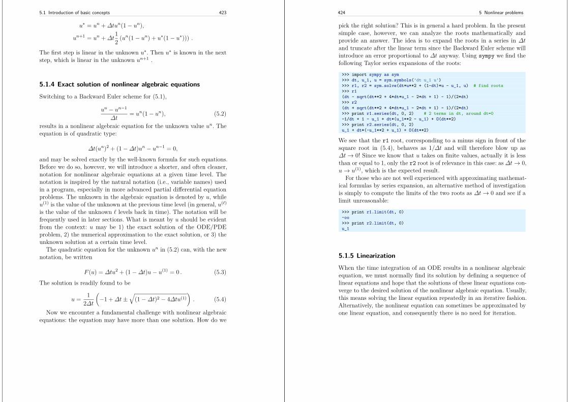
5.1 Introduction of basic concepts 423
u∗ = un +∆tun(1− un),
un+1 = un +∆t12 (un(1− un) + u∗(1− u∗))) .
The first step is linear in the unknown u∗. Then u∗ is known in the nextstep, which is linear in the unknown un+1 .
5.1.4 Exact solution of nonlinear algebraic equations
Switching to a Backward Euler scheme for (5.1),
un − un−1
∆t= un(1− un), (5.2)
results in a nonlinear algebraic equation for the unknown value un. Theequation is of quadratic type:
∆t(un)2 + (1−∆t)un − un−1 = 0,
and may be solved exactly by the well-known formula for such equations.Before we do so, however, we will introduce a shorter, and often cleaner,notation for nonlinear algebraic equations at a given time level. Thenotation is inspired by the natural notation (i.e., variable names) usedin a program, especially in more advanced partial differential equationproblems. The unknown in the algebraic equation is denoted by u, whileu(1) is the value of the unknown at the previous time level (in general, u(`)
is the value of the unknown ` levels back in time). The notation will befrequently used in later sections. What is meant by u should be evidentfrom the context: u may be 1) the exact solution of the ODE/PDEproblem, 2) the numerical approximation to the exact solution, or 3) theunknown solution at a certain time level.
The quadratic equation for the unknown un in (5.2) can, with the newnotation, be written
F (u) = ∆tu2 + (1−∆t)u− u(1) = 0 . (5.3)
The solution is readily found to be
u = 12∆t
(−1 +∆t±
√(1−∆t)2 − 4∆tu(1)
). (5.4)
Now we encounter a fundamental challenge with nonlinear algebraicequations: the equation may have more than one solution. How do we
424 5 Nonlinear problems
pick the right solution? This is in general a hard problem. In the presentsimple case, however, we can analyze the roots mathematically andprovide an answer. The idea is to expand the roots in a series in ∆tand truncate after the linear term since the Backward Euler scheme willintroduce an error proportional to ∆t anyway. Using sympy we find thefollowing Taylor series expansions of the roots:
>>> import sympy as sym>>> dt, u_1, u = sym.symbols(’dt u_1 u’)>>> r1, r2 = sym.solve(dt*u**2 + (1-dt)*u - u_1, u) # find roots>>> r1(dt - sqrt(dt**2 + 4*dt*u_1 - 2*dt + 1) - 1)/(2*dt)>>> r2(dt + sqrt(dt**2 + 4*dt*u_1 - 2*dt + 1) - 1)/(2*dt)>>> print r1.series(dt, 0, 2) # 2 terms in dt, around dt=0-1/dt + 1 - u_1 + dt*(u_1**2 - u_1) + O(dt**2)>>> print r2.series(dt, 0, 2)u_1 + dt*(-u_1**2 + u_1) + O(dt**2)
We see that the r1 root, corresponding to a minus sign in front of thesquare root in (5.4), behaves as 1/∆t and will therefore blow up as∆t→ 0! Since we know that u takes on finite values, actually it is lessthan or equal to 1, only the r2 root is of relevance in this case: as ∆t→ 0,u→ u(1), which is the expected result.
For those who are not well experienced with approximating mathemat-ical formulas by series expansion, an alternative method of investigationis simply to compute the limits of the two roots as ∆t→ 0 and see if alimit unreasonable:
>>> print r1.limit(dt, 0)-oo>>> print r2.limit(dt, 0)u_1
5.1.5 Linearization
When the time integration of an ODE results in a nonlinear algebraicequation, we must normally find its solution by defining a sequence oflinear equations and hope that the solutions of these linear equations con-verge to the desired solution of the nonlinear algebraic equation. Usually,this means solving the linear equation repeatedly in an iterative fashion.Alternatively, the nonlinear equation can sometimes be approximated byone linear equation, and consequently there is no need for iteration.
5.1 Introduction of basic concepts 425
Constructing a linear equation from a nonlinear one requires lineariza-tion of each nonlinear term. This can be done manually as in Picarditeration, or fully algorithmically as in Newton’s method. Examples willbest illustrate how to linearize nonlinear problems.
5.1.6 Picard iterationLet us write (5.3) in a more compact form
F (u) = au2 + bu+ c = 0,
with a = ∆t, b = 1 − ∆t, and c = −u(1). Let u− be an availableapproximation of the unknown u. Then we can linearize the term u2
simply by writing u−u. The resulting equation, F (u) = 0, is now linearand hence easy to solve:
F (u) ≈ F (u) = au−u+ bu+ c = 0 .
Since the equation F = 0 is only approximate, the solution u does notequal the exact solution ue of the exact equation F (ue) = 0, but we canhope that u is closer to ue than u− is, and hence it makes sense to repeatthe procedure, i.e., set u− = u and solve F (u) = 0 again. There is noguarantee that u is closer to ue than u−, but this approach has provento be effective in a wide range of applications.
The idea of turning a nonlinear equation into a linear one by using anapproximation u− of u in nonlinear terms is a widely used approach thatgoes under many names: fixed-point iteration, the method of successivesubstitutions, nonlinear Richardson iteration, and Picard iteration. Wewill stick to the latter name.
Picard iteration for solving the nonlinear equation arising from theBackward Euler discretization of the logistic equation can be written as
u = − c
au− + b, u− ← u .
The ← symbols means assignment (we set u− equal to the value of u).The iteration is started with the value of the unknown at the previoustime level: u− = u(1).
Some prefer an explicit iteration counter as superscript in the mathe-matical notation. Let uk be the computed approximation to the solutionin iteration k. In iteration k + 1 we want to solve
426 5 Nonlinear problems
aukuk+1 + buk+1 + c = 0 ⇒ uk+1 = − c
auk + b, k = 0, 1, . . .
Since we need to perform the iteration at every time level, the time levelcounter is often also included:
aun,kun,k+1+bun,k+1−un−1 = 0 ⇒ un,k+1 = un
aun,k + b, k = 0, 1, . . . ,
with the start value un,0 = un−1 and the final converged value un = un,k
for sufficiently large k.However, we will normally apply a mathematical notation in our final
formulas that is as close as possible to what we aim to write in a computercode and then it becomes natural to use u and u− instead of uk+1 anduk or un,k+1 and un,k.
Stopping criteria. The iteration method can typically be terminatedwhen the change in the solution is smaller than a tolerance εu:
|u− u−| ≤ εu,
or when the residual in the equation is sufficiently small (< εr),
|F (u)| = |au2 + bu+ c| < εr .
A single Picard iteration. Instead of iterating until a stopping criterionis fulfilled, one may iterate a specific number of times. Just one Picarditeration is popular as this corresponds to the intuitive idea of approx-imating a nonlinear term like (un)2 by un−1un. This follows from thelinearization u−un and the initial choice of u− = un−1 at time level tn. Inother words, a single Picard iteration corresponds to using the solutionat the previous time level to linearize nonlinear terms. The resultingdiscretization becomes (using proper values for a, b, and c)
un − un−1
∆t= un(1− un−1), (5.5)
which is a linear algebraic equation in the unknown un, making it easyto solve for un without any need for any alternative notation.
We shall later refer to the strategy of taking one Picard step, orequivalently, linearizing terms with use of the solution at the previoustime step, as the Picard1 method. It is a widely used approach in science
5.1 Introduction of basic concepts 427
and technology, but with some limitations if ∆t is not sufficiently small(as will be illustrated later).
NoticeEquation (5.5) does not correspond to a “pure” finite differencemethod where the equation is sampled at a point and derivativesreplaced by differences (because the un−1 term on the right-handside must then be un). The best interpretation of the scheme (5.5)is a Backward Euler difference combined with a single (perhapsinsufficient) Picard iteration at each time level, with the value atthe previous time level as start for the Picard iteration.
5.1.7 Linearization by a geometric mean
We consider now a Crank-Nicolson discretization of (5.1). This meansthat the time derivative is approximated by a centered difference,
[Dtu = u(1− u)]n+ 12 ,
written out as
un+1 − un∆t
= un+ 12 − (un+ 1
2 )2 . (5.6)
The term un+ 12 is normally approximated by an arithmetic mean,
un+ 12 ≈ 1
2(un + un+1),
such that the scheme involves the unknown function only at the timelevels where we actually compute it. The same arithmetic mean appliedto the nonlinear term gives
(un+ 12 )2 ≈ 1
4(un + un+1)2,
which is nonlinear in the unknown un+1. However, using a geometricmean for (un+ 1
2 )2 is a way of linearizing the nonlinear term in (5.6):
(un+ 12 )2 ≈ unun+1 .
428 5 Nonlinear problems
Using an arithmetic mean on the linear un+ 12 term in (5.6) and a geometric
mean for the second term, results in a linearized equation for the unknownun+1:
un+1 − un∆t
= 12(un + un+1) + unun+1,
which can readily be solved:
un+1 =1 + 1
2∆t
1 +∆tun − 12∆t
un .
This scheme can be coded directly, and since there is no nonlinearalgebraic equation to iterate over, we skip the simplified notation with ufor un+1 and u(1) for un. The technique with using a geometric averageis an example of transforming a nonlinear algebraic equation to a linearone, without any need for iterations.
The geometric mean approximation is often very effective for lineariz-ing quadratic nonlinearities. Both the arithmetic and geometric meanapproximations have truncation errors of order ∆t2 and are thereforecompatible with the truncation error O(∆t2) of the centered differenceapproximation for u′ in the Crank-Nicolson method.
Applying the operator notation for the means and finite differences,the linearized Crank-Nicolson scheme for the logistic equation can becompactly expressed as
[Dtu = ut + u2t,g]n+ 12 .
RemarkIf we use an arithmetic instead of a geometric mean for the nonlinearterm in (5.6), we end up with a nonlinear term (un+1)2. This termcan be linearized as u−un+1 in a Picard iteration approach and inparticular as unun+1 in a Picard1 iteration approach. The lattergives a scheme almost identical to the one arising from a geometricmean (the difference in un+1 being 1
4∆tun(un+1 − un) ≈ 1
4∆t2u′u,
i.e., a difference of size ∆t2).
5.1 Introduction of basic concepts 429
5.1.8 Newton’s method
The Backward Euler scheme (5.2) for the logistic equation leads to anonlinear algebraic equation (5.3). Now we write any nonlinear algebraicequation in the general and compact form
F (u) = 0 .
Newton’s method linearizes this equation by approximating F (u) by itsTaylor series expansion around a computed value u− and keeping onlythe linear part:
F (u) = F (u−) + F ′(u−)(u− u−) + 12F′′(u−)(u− u−)2 + · · ·
≈ F (u−) + F ′(u−)(u− u−) = F (u) .
The linear equation F (u) = 0 has the solution
u = u− − F (u−)F ′(u−) .
Expressed with an iteration index in the unknown, Newton’s methodtakes on the more familiar mathematical form
uk+1 = uk − F (uk)F ′(uk) , k = 0, 1, . . .
It can be shown that the error in iteration k + 1 of Newton’s methodis proportional to the square of the error in iteration k, a result referredto as quadratic convergence. This means that for small errors the methodconverges very fast, and in particular much faster than Picard iterationand other iteration methods. (The proof of this result is found in mosttextbooks on numerical analysis.) However, the quadratic convergenceappears only if uk is sufficiently close to the solution. Further away fromthe solution the method can easily converge very slowly or diverge. Thereader is encouraged to do Exercise 5.3 to get a better understanding forthe behavior of the method.
Application of Newton’s method to the logistic equation discretizedby the Backward Euler method is straightforward as we have
F (u) = au2 + bu+ c, a = ∆t, b = 1−∆t, c = −u(1),
and then
430 5 Nonlinear problems
F ′(u) = 2au+ b .
The iteration method becomes
u = u− + a(u−)2 + bu− + c
2au− + b, u− ← u . (5.7)
At each time level, we start the iteration by setting u− = u(1). Stoppingcriteria as listed for the Picard iteration can be used also for Newton’smethod.
An alternative mathematical form, where we write out a, b, and c, anduse a time level counter n and an iteration counter k, takes the form
un,k+1 = un,k + ∆t(un,k)2 + (1−∆t)un,k − un−1
2∆tun,k + 1−∆t , un,0 = un−1, (5.8)
for k = 0, 1, . . .. A program implementation is much closer to (5.7) thanto (5.8), but the latter is better aligned with the established mathematicalnotation used in the literature.
5.1.9 Relaxation
One iteration in Newton’s method or Picard iteration consists of solving alinear problem F (u) = 0. Sometimes convergence problems arise becausethe new solution u of F (u) = 0 is “too far away” from the previouslycomputed solution u−. A remedy is to introduce a relaxation, meaningthat we first solve F (u∗) = 0 for a suggested value u∗ and then we take uas a weighted mean of what we had, u−, and what our linearized equationF = 0 suggests, u∗:
u = ωu∗ + (1− ω)u− .
The parameter ω is known as a relaxation parameter, and a choice ω < 1may prevent divergent iterations.
Relaxation in Newton’s method can be directly incorporated in thebasic iteration formula:
u = u− − ω F (u−)F ′(u−) . (5.9)
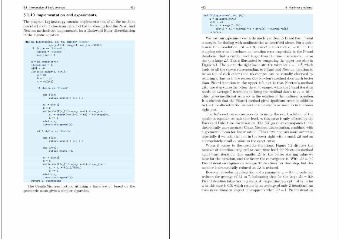
5.1 Introduction of basic concepts 431
5.1.10 Implementation and experimentsThe program logistic.py contains implementations of all the methodsdescribed above. Below is an extract of the file showing how the Picard andNewton methods are implemented for a Backward Euler discretizationof the logistic equation.
def BE_logistic(u0, dt, Nt, choice=’Picard’,eps_r=1E-3, omega=1, max_iter=1000):
if choice == ’Picard1’:choice = ’Picard’max_iter = 1
u = np.zeros(Nt+1)iterations = []u[0] = u0for n in range(1, Nt+1):
a = dtb = 1 - dtc = -u[n-1]
if choice == ’Picard’:
def F(u):return a*u**2 + b*u + c
u_ = u[n-1]k = 0while abs(F(u_)) > eps_r and k < max_iter:
u_ = omega*(-c/(a*u_ + b)) + (1-omega)*u_k += 1
u[n] = u_iterations.append(k)
elif choice == ’Newton’:
def F(u):return a*u**2 + b*u + c
def dF(u):return 2*a*u + b
u_ = u[n-1]k = 0while abs(F(u_)) > eps_r and k < max_iter:
u_ = u_ - F(u_)/dF(u_)k += 1
u[n] = u_iterations.append(k)
return u, iterations
The Crank-Nicolson method utilizing a linearization based on thegeometric mean gives a simpler algorithm:
432 5 Nonlinear problems
def CN_logistic(u0, dt, Nt):u = np.zeros(Nt+1)u[0] = u0for n in range(0, Nt):
u[n+1] = (1 + 0.5*dt)/(1 + dt*u[n] - 0.5*dt)*u[n]return u
Wemay run experiments with the model problem (5.1) and the differentstrategies for dealing with nonlinearities as described above. For a quitecoarse time resolution, ∆t = 0.9, use of a tolerance εr = 0.1 in thestopping criterion introduces an iteration error, especially in the Picarditerations, that is visibly much larger than the time discretization errordue to a large ∆t. This is illustrated by comparing the upper two plots inFigure 5.1. The one to the right has a stricter tolerance ε = 10−3, whichleads to all the curves corresponding to Picard and Newton iteration tobe on top of each other (and no changes can be visually observed byreducing εr further). The reason why Newton’s method does much betterthan Picard iteration in the upper left plot is that Newton’s methodwith one step comes far below the εr tolerance, while the Picard iterationneeds on average 7 iterations to bring the residual down to εr = 10−1,which gives insufficient accuracy in the solution of the nonlinear equation.It is obvious that the Picard1 method gives significant errors in additionto the time discretization unless the time step is as small as in the lowerright plot.
The BE exact curve corresponds to using the exact solution of thequadratic equation at each time level, so this curve is only affected by theBackward Euler time discretization. The CN gm curve corresponds to thetheoretically more accurate Crank-Nicolson discretization, combined witha geometric mean for linearization. This curve appears more accurate,especially if we take the plot in the lower right with a small ∆t and anappropriately small εr value as the exact curve.
When it comes to the need for iterations, Figure 5.2 displays thenumber of iterations required at each time level for Newton’s methodand Picard iteration. The smaller ∆t is, the better starting value wehave for the iteration, and the faster the convergence is. With ∆t = 0.9Picard iteration requires on average 32 iterations per time step, but thisnumber is dramatically reduced as ∆t is reduced.
However, introducing relaxation and a parameter ω = 0.8 immediatelyreduces the average of 32 to 7, indicating that for the large ∆t = 0.9,Picard iteration takes too long steps. An approximately optimal value forω in this case is 0.5, which results in an average of only 2 iterations! Aneven more dramatic impact of ω appears when ∆t = 1: Picard iteration
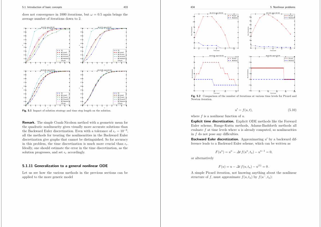
5.1 Introduction of basic concepts 433
does not convergence in 1000 iterations, but ω = 0.5 again brings theaverage number of iterations down to 2.
0 1 2 3 4 5 6 7 8 9t
0.1
0.2
0.3
0.4
0.5
0.6
0.7
0.8
0.9
1.0
u
dt=0.9, eps=5E-02
FEBE exactBE PicardBE Picard1BE NewtonCN gm
0 1 2 3 4 5 6 7 8 9t
0.1
0.2
0.3
0.4
0.5
0.6
0.7
0.8
0.9
1.0
u
dt=0.9, eps=1E-03
FEBE exactBE PicardBE Picard1BE NewtonCN gm
0 1 2 3 4 5 6 7 8 9t
0.1
0.2
0.3
0.4
0.5
0.6
0.7
0.8
0.9
1.0
u
dt=0.45, eps=1E-03
FEBE exactBE PicardBE Picard1BE NewtonCN gm
0 1 2 3 4 5 6 7 8 9t
0.1
0.2
0.3
0.4
0.5
0.6
0.7
0.8
0.9
1.0
u
dt=0.09, eps=1E-04
FEBE exactBE PicardBE Picard1BE NewtonCN gm
Fig. 5.1 Impact of solution strategy and time step length on the solution.
Remark. The simple Crank-Nicolson method with a geometric mean forthe quadratic nonlinearity gives visually more accurate solutions thanthe Backward Euler discretization. Even with a tolerance of εr = 10−3,all the methods for treating the nonlinearities in the Backward Eulerdiscretization give graphs that cannot be distinguished. So for accuracyin this problem, the time discretization is much more crucial than εr.Ideally, one should estimate the error in the time discretization, as thesolution progresses, and set εr accordingly.
5.1.11 Generalization to a general nonlinear ODELet us see how the various methods in the previous sections can beapplied to the more generic model
434 5 Nonlinear problems
2 4 6 8 10Time level
0
2
4
6
8
10
12
No o
f ite
ratio
ns
dt=0.9, eps=5E-02
PicardNewton
2 4 6 8 10Time level
0
5
10
15
20
25
30
35
40
No o
f ite
ratio
ns
dt=0.9, eps=1E-03
PicardNewton
5 10 15 20Time level
0
1
2
3
4
5
6
No o
f ite
ratio
ns
dt=0.45, eps=1E-03
PicardNewton
20 40 60 80 100Time level
0.0
0.5
1.0
1.5
2.0
2.5
3.0
No o
f ite
ratio
ns
dt=0.09, eps=1E-04
PicardNewton
Fig. 5.2 Comparison of the number of iterations at various time levels for Picard andNewton iteration.
u′ = f(u, t), (5.10)
where f is a nonlinear function of u.Explicit time discretization. Explicit ODE methods like the ForwardEuler scheme, Runge-Kutta methods, Adams-Bashforth methods allevaluate f at time levels where u is already computed, so nonlinearitiesin f do not pose any difficulties.Backward Euler discretization. Approximating u′ by a backward dif-ference leads to a Backward Euler scheme, which can be written as
F (un) = un −∆t f(un, tn)− un−1 = 0,
or alternatively
F (u) = u−∆t f(u, tn)− u(1) = 0 .
A simple Picard iteration, not knowing anything about the nonlinearstructure of f , must approximate f(u, tn) by f(u−, tn):
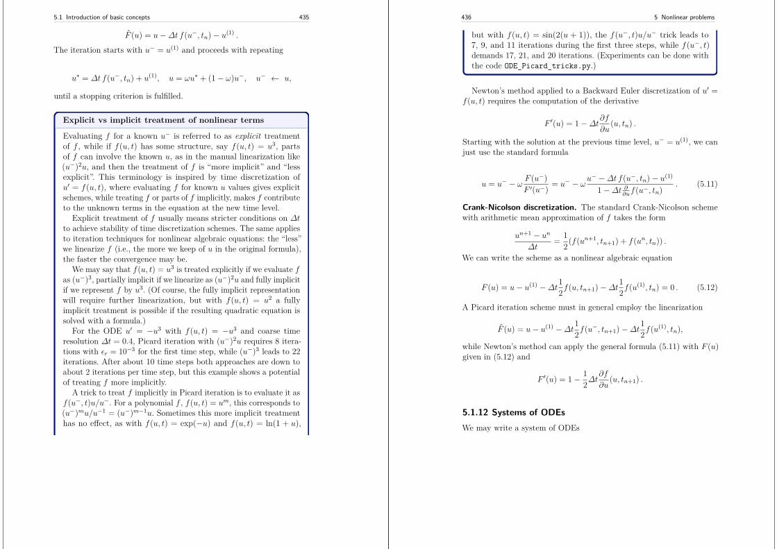
5.1 Introduction of basic concepts 435
F (u) = u−∆t f(u−, tn)− u(1) .
The iteration starts with u− = u(1) and proceeds with repeating
u∗ = ∆t f(u−, tn) + u(1), u = ωu∗ + (1− ω)u−, u− ← u,
until a stopping criterion is fulfilled.
Explicit vs implicit treatment of nonlinear terms
Evaluating f for a known u− is referred to as explicit treatmentof f , while if f(u, t) has some structure, say f(u, t) = u3, partsof f can involve the known u, as in the manual linearization like(u−)2u, and then the treatment of f is “more implicit” and “lessexplicit”. This terminology is inspired by time discretization ofu′ = f(u, t), where evaluating f for known u values gives explicitschemes, while treating f or parts of f implicitly, makes f contributeto the unknown terms in the equation at the new time level.
Explicit treatment of f usually means stricter conditions on ∆tto achieve stability of time discretization schemes. The same appliesto iteration techniques for nonlinear algebraic equations: the “less”we linearize f (i.e., the more we keep of u in the original formula),the faster the convergence may be.
We may say that f(u, t) = u3 is treated explicitly if we evaluate fas (u−)3, partially implicit if we linearize as (u−)2u and fully implicitif we represent f by u3. (Of course, the fully implicit representationwill require further linearization, but with f(u, t) = u2 a fullyimplicit treatment is possible if the resulting quadratic equation issolved with a formula.)
For the ODE u′ = −u3 with f(u, t) = −u3 and coarse timeresolution ∆t = 0.4, Picard iteration with (u−)2u requires 8 itera-tions with εr = 10−3 for the first time step, while (u−)3 leads to 22iterations. After about 10 time steps both approaches are down toabout 2 iterations per time step, but this example shows a potentialof treating f more implicitly.
A trick to treat f implicitly in Picard iteration is to evaluate it asf(u−, t)u/u−. For a polynomial f , f(u, t) = um, this corresponds to(u−)mu/u−1 = (u−)m−1u. Sometimes this more implicit treatmenthas no effect, as with f(u, t) = exp(−u) and f(u, t) = ln(1 + u),
436 5 Nonlinear problems
but with f(u, t) = sin(2(u + 1)), the f(u−, t)u/u− trick leads to7, 9, and 11 iterations during the first three steps, while f(u−, t)demands 17, 21, and 20 iterations. (Experiments can be done withthe code ODE_Picard_tricks.py.)
Newton’s method applied to a Backward Euler discretization of u′ =f(u, t) requires the computation of the derivative
F ′(u) = 1−∆t∂f∂u
(u, tn) .
Starting with the solution at the previous time level, u− = u(1), we canjust use the standard formula
u = u− − ω F (u−)F ′(u−) = u− − ωu
− −∆t f(u−, tn)− u(1)
1−∆t ∂∂uf(u−, tn). (5.11)
Crank-Nicolson discretization. The standard Crank-Nicolson schemewith arithmetic mean approximation of f takes the form
un+1 − un∆t
= 12(f(un+1, tn+1) + f(un, tn)) .
We can write the scheme as a nonlinear algebraic equation
F (u) = u− u(1) −∆t12f(u, tn+1)−∆t12f(u(1), tn) = 0 . (5.12)
A Picard iteration scheme must in general employ the linearization
F (u) = u− u(1) −∆t12f(u−, tn+1)−∆t12f(u(1), tn),
while Newton’s method can apply the general formula (5.11) with F (u)given in (5.12) and
F ′(u) = 1− 12∆t
∂f
∂u(u, tn+1) .
5.1.12 Systems of ODEsWe may write a system of ODEs
5.1 Introduction of basic concepts 437
d
dtu0(t) = f0(u0(t), u1(t), . . . , uN (t), t),
d
dtu1(t) = f1(u0(t), u1(t), . . . , uN (t), t),
...d
dtum(t) = fm(u0(t), u1(t), . . . , uN (t), t),
as
u′ = f(u, t), u(0) = U0, (5.13)
if we interpret u as a vector u = (u0(t), u1(t), . . . , uN (t)) and f as avector function with components (f0(u, t), f1(u, t), . . . , fN (u, t)).
Most solution methods for scalar ODEs, including the Forward andBackward Euler schemes and the Crank-Nicolson method, generalizein a straightforward way to systems of ODEs simply by using vectorarithmetics instead of scalar arithmetics, which corresponds to applyingthe scalar scheme to each component of the system. For example, here isa backward difference scheme applied to each component,
un0 − un−10
∆t= f0(un, tn),
un1 − un−11
∆t= f1(un, tn),...
unN − un−1N
∆t= fN (un, tn),
which can be written more compactly in vector form as
un − un−1
∆t= f(un, tn) .
This is a system of algebraic equations,
un −∆t f(un, tn)− un−1 = 0,
or written out
438 5 Nonlinear problems
un0 −∆t f0(un, tn)− un−10 = 0,
...unN −∆t fN (un, tn)− un−1
N = 0 .
Example. We shall address the 2× 2 ODE system for oscillations of apendulum subject to gravity and air drag. The system can be written as
ω = − sin θ − βω|ω|, (5.14)θ = ω, (5.15)
where β is a dimensionless parameter (this is the scaled, dimensionlessversion of the original, physical model). The unknown components of thesystem are the angle θ(t) and the angular velocity ω(t). We introduceu0 = ω and u1 = θ, which leads to
u′0 = f0(u, t) = − sin u1 − βu0|u0|,u′1 = f1(u, t) = u0 .
A Crank-Nicolson scheme reads
un+10 − un0∆t
= − sin un+ 12
1 − βun+ 12
0 |un+ 12
0 |
≈ − sin(1
2(un+11 + u1n)
)− β 1
4(un+10 + un0 )|un+1
0 + un0 |,(5.16)
un+11 − un1∆t
= un+ 1
20 ≈ 1
2(un+10 + un0 ) . (5.17)
This is a coupled system of two nonlinear algebraic equations in twounknowns un+1
0 and un+11 .
Using the notation u0 and u1 for the unknowns un+10 and un+1
1 inthis system, writing u
(1)0 and u
(1)1 for the previous values un0 and un1 ,
multiplying by ∆t and moving the terms to the left-hand sides, gives
5.2 Systems of nonlinear algebraic equations 439
u0 − u(1)0 +∆t sin
(12(u1 + u
(1)1 ))
+ 14∆tβ(u0 + u
(1)0 )|u0 + u
(1)0 | = 0,
(5.18)
u1 − u(1)1 −
12∆t(u0 + u
(1)0 ) = 0 .
(5.19)
Obviously, we have a need for solving systems of nonlinear algebraicequations, which is the topic of the next section.
5.2 Systems of nonlinear algebraic equations
Implicit time discretization methods for a system of ODEs, or a PDE,lead to systems of nonlinear algebraic equations, written compactly as
F (u) = 0,
where u is a vector of unknowns u = (u0, . . . , uN ), and F is a vectorfunction: F = (F0, . . . , FN ). The system at the end of Section 5.1.12 fitsthis notation with N = 2, F0(u) given by the left-hand side of (5.18),while F1(u) is the left-hand side of (5.19).
Sometimes the equation system has a special structure because of theunderlying problem, e.g.,
A(u)u = b(u),
with A(u) as an (N + 1)× (N + 1) matrix function of u and b as a vectorfunction: b = (b0, . . . , bN ).
We shall next explain how Picard iteration and Newton’s method canbe applied to systems like F (u) = 0 and A(u)u = b(u). The expositionhas a focus on ideas and practical computations. More theoretical con-siderations, including quite general results on convergence properties ofthese methods, can be found in Kelley [8].
5.2.1 Picard iteration
We cannot apply Picard iteration to nonlinear equations unless there issome special structure. For the commonly arising case A(u)u = b(u) wecan linearize the product A(u)u to A(u−)u and b(u) as b(u−). That is,
440 5 Nonlinear problems
we use the most previously computed approximation in A and b to arriveat a linear system for u:
A(u−)u = b(u−) .
A relaxed iteration takes the form
A(u−)u∗ = b(u−), u = ωu∗ + (1− ω)u− .
In other words, we solve a system of nonlinear algebraic equations as asequence of linear systems.
Algorithm for relaxed Picard iteration
Given A(u)u = b(u) and an initial guess u−, iterate until conver-gence:
1. solve A(u−)u∗ = b(u−) with respect to u∗2. u = ωu∗ + (1− ω)u−3. u− ← u
“Until convergence” means that the iteration is stopped when thechange in the unknown, ||u − u−||, or the residual ||A(u)u − b||, issufficiently small, see Section 5.2.3 for more details.
5.2.2 Newton’s methodThe natural starting point for Newton’s method is the general nonlinearvector equation F (u) = 0. As for a scalar equation, the idea is to approx-imate F around a known value u− by a linear function F , calculatedfrom the first two terms of a Taylor expansion of F . In the multi-variatecase these two terms become
F (u−) + J(u−) · (u− u−),
where J is the Jacobian of F , defined by
Ji,j = ∂Fi∂uj
.
So, the original nonlinear system is approximated by
5.2 Systems of nonlinear algebraic equations 441
F (u) = F (u−) + J(u−) · (u− u−) = 0,
which is linear in u and can be solved in a two-step procedure: firstsolve Jδu = −F (u−) with respect to the vector δu and then updateu = u− + δu. A relaxation parameter can easily be incorporated:
u = ω(u− + δu) + (1− ω)u− = u− + ωδu .
Algorithm for Newton’s method
Given F (u) = 0 and an initial guess u−, iterate until convergence:
1. solve Jδu = −F (u−) with respect to δu2. u = u− + ωδu3. u− ← u
For the special system with structure A(u)u = b(u),
Fi =∑
k
Ai,k(u)uk − bi(u),
one gets
Ji,j =∑
k
∂Ai,k∂uj
uk + Ai,j −∂bi∂uj
. (5.20)
We realize that the Jacobian needed in Newton’s method consists ofA(u−) as in the Picard iteration plus two additional terms arising fromthe differentiation. Using the notation A′(u) for ∂A/∂u (a quantity withthree indices: ∂Ai,k/∂uj), and b′(u) for ∂b/∂u (a quantity with twoindices: ∂bi/∂uj), we can write the linear system to be solved as
(A+ A′u+ b′)δu = −Au+ b,
or
(A(u−) + A′(u−)u− + b′(u−))δu = −A(u−)u− + b(u−) .
Rearranging the terms demonstrates the difference from the systemsolved in each Picard iteration:
442 5 Nonlinear problems
A(u−)(u− + δu)− b(u−)︸ ︷︷ ︸Picard system
+ γ(A′(u−)u− + b′(u−))δu = 0 .
Here we have inserted a parameter γ such that γ = 0 gives the Picardsystem and γ = 1 gives the Newton system. Such a parameter can behandy in software to easily switch between the methods.
Combined algorithm for Picard and Newton iteration
Given A(u), b(u), and an initial guess u−, iterate until convergence:
1. solve (A+ γ(A′(u−)u− + b′(u−)))δu = −A(u−)u− + b(u−) withrespect to δu
2. u = u− + ωδu3. u− ← u
γ = 1 gives a Newton method while γ = 0 corresponds to Picarditeration.
5.2.3 Stopping criteria
Let || · || be the standard Euclidean vector norm. Four termination criteriaare much in use:
• Absolute change in solution: ||u− u−|| ≤ εu• Relative change in solution: ||u − u−|| ≤ εu||u0||, where u0 denotes
the start value of u− in the iteration• Absolute residual: ||F (u)|| ≤ εr• Relative residual: ||F (u)|| ≤ εr||F (u0)||
To prevent divergent iterations to run forever, one terminates the itera-tions when the current number of iterations k exceeds a maximum valuekmax.
The relative criteria are most used since they are not sensitive tothe characteristic size of u. Nevertheless, the relative criteria can bemisleading when the initial start value for the iteration is very closeto the solution, since an unnecessary reduction in the error measure isenforced. In such cases the absolute criteria work better. It is common
5.2 Systems of nonlinear algebraic equations 443
to combine the absolute and relative measures of the size of the residual,as in
||F (u)|| ≤ εrr||F (u0)||+ εra, (5.21)
where εrr is the tolerance in the relative criterion and εra is the tolerancein the absolute criterion. With a very good initial guess for the iteration(typically the solution of a differential equation at the previous timelevel), the term ||F (u0)|| is small and εra is the dominating tolerance.Otherwise, εrr||F (u0)|| and the relative criterion dominates.
With the change in solution as criterion we can formulate a combinedabsolute and relative measure of the change in the solution:
||δu|| ≤ εur||u0||+ εua, (5.22)
The ultimate termination criterion, combining the residual and thechange in solution with a test on the maximum number of iterations, canbe expressed as
||F (u)|| ≤ εrr||F (u0)||+ εra or ||δu|| ≤ εur||u0||+ εua or k > kmax .(5.23)
5.2.4 Example: A nonlinear ODE model from epidemiology
The simplest model spreading of a disease, such as a flu, takes the formof a 2× 2 ODE system
S′ = −βSI, (5.24)I ′ = βSI − νI, (5.25)
where S(t) is the number of people who can get ill (susceptibles) andI(t) is the number of people who are ill (infected). The constants β > 0and ν > 0 must be given along with initial conditions S(0) and I(0).
Implicit time discretization. A Crank-Nicolson scheme leads to a 2× 2system of nonlinear algebraic equations in the unknowns Sn+1 and In+1:
444 5 Nonlinear problems
Sn+1 − Sn∆t
= −β[SI]n+ 12 ≈ −β2 (SnIn + Sn+1In+1), (5.26)
In+1 − In∆t
= β[SI]n+ 12 − νIn+ 1
2 ≈ β
2 (SnIn + Sn+1In+1)− ν
2 (In + In+1) .(5.27)
Introducing S for Sn+1, S(1) for Sn, I for In+1, I(1) for In, we can rewritethe system as
FS(S, I) = S − S(1) + 12∆tβ(S(1)I(1) + SI) = 0, (5.28)
FI(S, I) = I − I(1) − 12∆tβ(S(1)I(1) + SI) + 1
2∆tν(I(1) + I) = 0 .(5.29)
A Picard iteration. We assume that we have approximations S− and I−to S and I, respectively. A way of linearizing the only nonlinear term SIis to write I−S in the FS = 0 equation and S−I in the FI = 0 equation,which also decouples the equations. Solving the resulting linear equationswith respect to the unknowns S and I gives
S =S(1) − 1
2∆tβS(1)I(1)
1 + 12∆tβI
− ,
I =I(1) + 1
2∆tβS(1)I(1) − 1
2∆tνI(1)
1− 12∆tβS
− + 12∆tν
.
Before a new iteration, we must update S− ← S and I− ← I.
Newton’s method. The nonlinear system (5.28)-(5.29) can be writtenas F (u) = 0 with F = (FS , FI) and u = (S, I). The Jacobian becomes
J =(
∂∂SFS
∂∂IFS
∂∂SFI
∂∂IFI
)=(
1 + 12∆tβI
12∆tβS
−12∆tβI 1− 1
2∆tβS + 12∆tν
).
The Newton system J(u−)δu = −F (u−) to be solved in each iteration isthen
5.3 Linearization at the differential equation level 445(
1 + 12∆tβI
− 12∆tβS
−
−12∆tβI
− 1− 12∆tβS
− + 12∆tν
)(δSδI
)=
(S− − S(1) + 1
2∆tβ(S(1)I(1) + S−I−)I− − I(1) − 1
2∆tβ(S(1)I(1) + S−I−) + 12∆tν(I(1) + I−)
)
Remark. For this particular system of ODEs, explicit time integrationmethods work very well. Even a Forward Euler scheme is fine, but (as alsoexperienced more generally) the 4-th order Runge-Kutta method is anexcellent balance between high accuracy, high efficiency, and simplicity.
5.3 Linearization at the differential equation level
The attention is now turned to nonlinear partial differential equations(PDEs) and application of the techniques explained above for ODEs. Themodel problem is a nonlinear diffusion equation for u(x, t):
∂u
∂t= ∇ · (α(u)∇u) + f(u), x ∈ Ω, t ∈ (0, T ], (5.30)
−α(u)∂u∂n
= g, x ∈ ∂ΩN , t ∈ (0, T ], (5.31)
u = u0, x ∈ ∂ΩD, t ∈ (0, T ] . (5.32)
In the present section, our aim is to discretize this problem in time andthen present techniques for linearizing the time-discrete PDE problem“at the PDE level” such that we transform the nonlinear stationary PDEproblem at each time level into a sequence of linear PDE problems, whichcan be solved using any method for linear PDEs. This strategy avoidsthe solution of systems of nonlinear algebraic equations. In Section 5.4we shall take the opposite (and more common) approach: discretize thenonlinear problem in time and space first, and then solve the resultingnonlinear algebraic equations at each time level by the methods ofSection 5.2. Very often, the two approaches are mathematically identical,so there is no preference from a computational efficiency point of view.The details of the ideas sketched above will hopefully become clearthrough the forthcoming examples.
446 5 Nonlinear problems
5.3.1 Explicit time integration
The nonlinearities in the PDE are trivial to deal with if we choose anexplicit time integration method for (5.30), such as the Forward Eulermethod:
[D+t u = ∇ · (α(u)∇u) + f(u)]n,
or written out,
un+1 − un∆t
= ∇ · (α(un)∇un) + f(un),
which is a linear equation in the unknown un+1 with solution
un+1 = un +∆t∇ · (α(un)∇un) +∆tf(un) .
The disadvantage with this discretization is the strict stability criterion∆t ≤ h2/(6 maxα) for the case f = 0 and a standard 2nd-order finitedifference discretization in 3D space with mesh cell sizes h = ∆x = ∆y =∆z.
5.3.2 Backward Euler scheme and Picard iteration
A Backward Euler scheme for (5.30) reads
[D−t u = ∇ · (α(u)∇u) + f(u)]n .
Written out,
un − un−1
∆t= ∇ · (α(un)∇un) + f(un) . (5.33)
This is a nonlinear PDE for the unknown function un(x). Such a PDEcan be viewed as a time-independent PDE where un−1(x) is a knownfunction.
We introduce a Picard iteration with k as iteration counter. A typicallinearization of the ∇ · (α(un)∇un) term in iteration k + 1 is to usethe previously computed un,k approximation in the diffusion coefficient:α(un,k). The nonlinear source term is treated similarly: f(un,k). Theunknown function un,k+1 then fulfills the linear PDE
un,k+1 − un−1
∆t= ∇ · (α(un,k)∇un,k+1) + f(un,k) . (5.34)
5.3 Linearization at the differential equation level 447
The initial guess for the Picard iteration at this time level can be takenas the solution at the previous time level: un,0 = un−1.
We can alternatively apply the implementation-friendly notation whereu corresponds to the unknown we want to solve for, i.e., un,k+1 above,and u− is the most recently computed value, un,k above. Moreover, u(1)
denotes the unknown function at the previous time level, un−1 above.The PDE to be solved in a Picard iteration then looks like
u− u(1)
∆t= ∇ · (α(u−)∇u) + f(u−) . (5.35)
At the beginning of the iteration we start with the value from the previoustime level: u− = u(1), and after each iteration, u− is updated to u.
Remark on notationThe previous derivations of the numerical scheme for time discretiza-tions of PDEs have, strictly speaking, a somewhat sloppy notation,but it is much used and convenient to read. A more precise notationmust distinguish clearly between the exact solution of the PDEproblem, here denoted ue(x, t), and the exact solution of the spatialproblem, arising after time discretization at each time level, where(5.33) is an example. The latter is here represented as un(x) and isan approximation to ue(x, tn). Then we have another approximationun,k(x) to un(x) when solving the nonlinear PDE problem for unby iteration methods, as in (5.34).
In our notation, u is a synonym for un,k+1 and u(1) is a synonymfor un−1, inspired by what are natural variable names in a code.We will usually state the PDE problem in terms of u and quicklyredefine the symbol u to mean the numerical approximation, whileue is not explicitly introduced unless we need to talk about theexact solution and the approximate solution at the same time.
5.3.3 Backward Euler scheme and Newton’s method
At time level n, we have to solve the stationary PDE (5.33). In theprevious section, we saw how this can be done with Picard iterations.Another alternative is to apply the idea of Newton’s method in a cleverway. Normally, Newton’s method is defined for systems of algebraic
448 5 Nonlinear problems
equations, but the idea of the method can be applied at the PDE leveltoo.
Linearization via Taylor expansions. Let un,k be an approximation tothe unknown un. We seek a better approximation on the form
un = un,k + δu . (5.36)
The idea is to insert (5.36) in (5.33), Taylor expand the nonlinearitiesand keep only the terms that are linear in δu (which makes (5.36) anapproximation for un). Then we can solve a linear PDE for the correctionδu and use (5.36) to find a new approximation
un,k+1 = un,k + δu
to un. Repeating this procedure gives a sequence un,k+1, k = 0, 1, . . .that hopefully converges to the goal un.
Let us carry out all the mathematical details for the nonlinear diffusionPDE discretized by the Backward Euler method. Inserting (5.36) in (5.33)gives
un,k + δu− un−1
∆t= ∇·(α(un,k+δu)∇(un,k+δu))+f(un,k+δu) . (5.37)
We can Taylor expand α(un,k + δu) and f(un,k + δu):
α(un,k + δu) = α(un,k) + dα
du(un,k)δu+O(δu2) ≈ α(un,k) + α′(un,k)δu,
f(un,k + δu) = f(un,k) + df
du(un,k)δu+O(δu2) ≈ f(un,k) + f ′(un,k)δu .
Inserting the linear approximations of α and f in (5.37) results in
un,k + δu− un−1
∆t= ∇ · (α(un,k)∇un,k) + f(un,k)+
∇ · (α(un,k)∇δu) +∇ · (α′(un,k)δu∇un,k)+∇ · (α′(un,k)δu∇δu) + f ′(un,k)δu . (5.38)
The term α′(un,k)δu∇δu is of order δu2 and therefore omitted sincewe expect the correction δu to be small (δu δu2). Reorganizing theequation gives a PDE for δu that we can write in short form as
5.3 Linearization at the differential equation level 449
δF (δu;un,k) = −F (un,k),
where
F (un,k) = un,k − un−1
∆t−∇ · (α(un,k)∇un,k) + f(un,k), (5.39)
δF (δu;un,k) = − 1∆t
δu+∇ · (α(un,k)∇δu)+
∇ · (α′(un,k)δu∇un,k) + f ′(un,k)δu . (5.40)
Note that δF is a linear function of δu, and F contains only terms thatare known, such that the PDE for δu is indeed linear.
ObservationsThe notational form δF = −F resembles the Newton systemJδu = −F for systems of algebraic equations, with δF as Jδu.The unknown vector in a linear system of algebraic equations entersthe system as a linear operator in terms of a matrix-vector product(Jδu), while at the PDE level we have a linear differential operatorinstead (δF ).
Similarity with Picard iteration. We can rewrite the PDE for δu in aslightly different way too if we define un,k + δu as un,k+1.
un,k+1 − un−1
∆t= ∇ · (α(un,k)∇un,k+1) + f(un,k)
+∇ · (α′(un,k)δu∇un,k) + f ′(un,k)δu . (5.41)
Note that the first line is the same PDE as arises in the Picard iteration,while the remaining terms arise from the differentiations that are aninherent ingredient in Newton’s method.
Implementation. For coding we want to introduce u for un, u− for un,kand u(1) for un−1. The formulas for F and δF are then more clearlywritten as
450 5 Nonlinear problems
F (u−) = u− − u(1)
∆t−∇ · (α(u−)∇u−) + f(u−), (5.42)
δF (δu;u−) = − 1∆t
δu+∇ · (α(u−)∇δu)+
∇ · (α′(u−)δu∇u−) + f ′(u−)δu . (5.43)
The form that orders the PDE as the Picard iteration terms plus theNewton method’s derivative terms becomes
u− u(1)
∆t= ∇ · (α(u−)∇u) + f(u−)+
γ(∇ · (α′(u−)(u− u−)∇u−) + f ′(u−)(u− u−)) . (5.44)
The Picard and full Newton versions correspond to γ = 0 and γ = 1,respectively.Derivation with alternative notation. Some may prefer to derive thelinearized PDE for δu using the more compact notation. We start withinserting un = u− + δu to get
u− + δu− un−1
∆t= ∇ · (α(u− + δu)∇(u− + δu)) + f(u− + δu) .
Taylor expanding,
α(u− + δu) ≈ α(u−) + α′(u−)δu,f(u− + δu) ≈ f(u−) + f ′(u−)δu,
and inserting these expressions gives a less cluttered PDE for δu:
u− + δu− un−1
∆t= ∇ · (α(u−)∇u−) + f(u−)+
∇ · (α(u−)∇δu) +∇ · (α′(u−)δu∇u−)+∇ · (α′(u−)δu∇δu) + f ′(u−)δu .
5.3.4 Crank-Nicolson discretizationA Crank-Nicolson discretization of (5.30) applies a centered difference attn+ 1
2:
5.4 1D stationary nonlinear differential equations 451
[Dtu = ∇ · (α(u)∇u) + f(u)]n+ 12 .
The standard technique is to apply an arithmetic average for quantitiesdefined between two mesh points, e.g.,
un+ 12 ≈ 1
2(un + un+1) .
However, with nonlinear terms we have many choices of formulating anarithmetic mean:
[f(u)]n+ 12 ≈ f(1
2(un + un+1)) = [f(ut)]n+ 12 , (5.45)
[f(u)]n+ 12 ≈ 1
2(f(un) + f(un+1)) = [f(u)t]n+ 12 , (5.46)
[α(u)∇u]n+ 12 ≈ α(1
2(un + un+1))∇(12(un + un+1)) = [α(ut)∇ut]n+ 1
2 ,
(5.47)
[α(u)∇u]n+ 12 ≈ 1
2(α(un) + α(un+1))∇(12(un + un+1)) = [α(u)t∇ut]n+ 1
2 ,
(5.48)
[α(u)∇u]n+ 12 ≈ 1
2(α(un)∇un + α(un+1)∇un+1) = [α(u)∇ut]n+ 12 .
(5.49)
A big question is whether there are significant differences in accuracybetween taking the products of arithmetic means or taking the arithmeticmean of products. Exercise 5.6 investigates this question, and the answeris that the approximation is O(∆t2) in both cases.
5.4 1D stationary nonlinear differential equations
Section 5.3 presented methods for linearizing time-discrete PDEs directlyprior to discretization in space. We can alternatively carry out thediscretization in space of the time-discrete nonlinear PDE problem andget a system of nonlinear algebraic equations, which can be solved byPicard iteration or Newton’s method as presented in Section 5.2. Thislatter approach will now be described in detail.
We shall work with the 1D problem
452 5 Nonlinear problems
− (α(u)u′)′ + au = f(u), x ∈ (0, L), α(u(0))u′(0) = C, u(L) = D .(5.50)
The problem (5.50) arises from the stationary limit of a diffusionequation,
∂u
∂t= ∂
∂x
(α(u)∂u
∂x
)− au+ f(u), (5.51)
as t → ∞ and ∂u/∂t → 0. Alternatively, the problem (5.50) arises ateach time level from implicit time discretization of (5.51). For example,a Backward Euler scheme for (5.51) leads to
un − un−1
∆t= d
dx
(α(un)du
n
dx
)− aun + f(un) . (5.52)
Introducing u(x) for un(x), u(1) for un−1, and defining f(u) in (5.50) tobe f(u) in (5.52) plus un−1/∆t, gives (5.50) with a = 1/∆t.
5.4.1 Finite difference discretization
The nonlinearity in the differential equation (5.50) poses no more difficultythan a variable coefficient, as in the term (α(x)u′)′. We can therefore usea standard finite difference approach to discretizing the Laplace termwith a variable coefficient:
[−DxαDxu+ au = f ]i .
Writing this out for a uniform mesh with points xi = i∆x, i = 0, . . . , Nx,leads to
− 1∆x2
(αi+ 1
2(ui+1 − ui)− αi− 1
2(ui − ui−1)
)+ aui = f(ui) . (5.53)
This equation is valid at all the mesh points i = 0, 1, . . . , Nx − 1. Ati = Nx we have the Dirichlet condition ui = 0. The only difference fromthe case with (α(x)u′)′ and f(x) is that now α and f are functions of uand not only of x: (α(u(x))u′)′ and f(u(x)).
The quantity αi+ 12, evaluated between two mesh points, needs a com-
ment. Since α depends on u and u is only known at the mesh points, weneed to express αi+ 1
2in terms of ui and ui+1. For this purpose we use
an arithmetic mean, although a harmonic mean is also common in this
5.4 1D stationary nonlinear differential equations 453
context if α features large jumps. There are two choices of arithmeticmeans:
αi+ 12≈ α(1
2(ui + ui+1) = [α(ux)]i+ 12 , (5.54)
αi+ 12≈ 1
2(α(ui) + α(ui+1)) = [α(u)x]i+ 12 (5.55)
Equation (5.53) with the latter approximation then looks like
− 12∆x2 ((α(ui) + α(ui+1))(ui+1 − ui)− (α(ui−1) + α(ui))(ui − ui−1))
+ aui = f(ui), (5.56)
or written more compactly,
[−DxαxDxu+ au = f ]i .
At mesh point i = 0 we have the boundary condition α(u)u′ = C,which is discretized by
[α(u)D2xu = C]0,
meaning
α(u0)u1 − u−12∆x = C . (5.57)
The fictitious value u−1 can be eliminated with the aid of (5.56) for i = 0.Formally, (5.56) should be solved with respect to ui−1 and that value(for i = 0) should be inserted in (5.57), but it is algebraically much easierto do it the other way around. Alternatively, one can use a ghost cell[−∆x, 0] and update the u−1 value in the ghost cell according to (5.57)after every Picard or Newton iteration. Such an approach means that weuse a known u−1 value in (5.56) from the previous iteration.
5.4.2 Solution of algebraic equations
The structure of the equation system. The nonlinear algebraic equa-tions (5.56) are of the form A(u)u = b(u) with
454 5 Nonlinear problems
Ai,i = 12∆x2 (α(ui−1) + 2α(ui)α(ui+1)) + a,
Ai,i−1 = − 12∆x2 (α(ui−1) + α(ui)),
Ai,i+1 = − 12∆x2 (α(ui) + α(ui+1)),
bi = f(ui) .
The matrix A(u) is tridiagonal: Ai,j = 0 for j > i+ 1 and j < i− 1.The above expressions are valid for internal mesh points 1 ≤ i ≤ Nx−1.
For i = 0 we need to express ui−1 = u−1 in terms of u1 using (5.57):
u−1 = u1 −2∆xα(u0)C . (5.58)
This value must be inserted in A0,0. The expression for Ai,i+1 applies fori = 0, and Ai,i−1 does not enter the system when i = 0.
Regarding the last equation, its form depends on whether we includethe Dirichlet condition u(L) = D, meaning uNx = D, in the nonlinearalgebraic equation system or not. Suppose we choose (u0, u1, . . . , uNx−1)as unknowns, later referred to as systems without Dirichlet conditions.The last equation corresponds to i = Nx − 1. It involves the boundaryvalue uNx , which is substituted by D. If the unknown vector includes theboundary value, (u0, u1, . . . , uNx), later referred to as system includingDirichlet conditions, the equation for i = Nx−1 just involves the unknownuNx , and the final equation becomes uNx = D, corresponding to Ai,i = 1and bi = D for i = Nx.
Picard iteration. The obvious Picard iteration scheme is to use previ-ously computed values of ui in A(u) and b(u), as described more in detailin Section 5.2. With the notation u− for the most recently computedvalue of u, we have the system F (u) ≈ F (u) = A(u−)u − b(u−), withF = (F0, F1, . . . , Fm), u = (u0, u1, . . . , um). The index m is Nx if thesystem includes the Dirichlet condition as a separate equation and Nx−1otherwise. The matrix A(u−) is tridiagonal, so the solution procedureis to fill a tridiagonal matrix data structure and the right-hand sidevector with the right numbers and call a Gaussian elimination routinefor tridiagonal linear systems.
Mesh with two cells. It helps on the understanding of the details towrite out all the mathematics in a specific case with a small mesh, sayjust two cells (Nx = 2). We use u−i for the i-th component in u−.
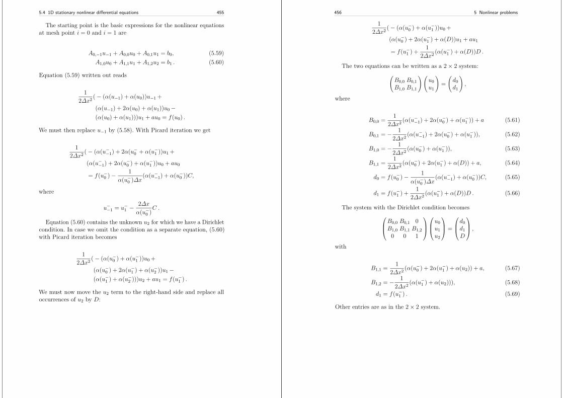
5.4 1D stationary nonlinear differential equations 455
The starting point is the basic expressions for the nonlinear equationsat mesh point i = 0 and i = 1 are
A0,−1u−1 + A0,0u0 + A0,1u1 = b0, (5.59)A1,0u0 + A1,1u1 + A1,2u2 = b1 . (5.60)
Equation (5.59) written out reads
12∆x2 (− (α(u−1) + α(u0))u−1 +
(α(u−1) + 2α(u0) + α(u1))u0−(α(u0) + α(u1)))u1 + au0 = f(u0) .
We must then replace u−1 by (5.58). With Picard iteration we get
12∆x2 (− (α(u−−1) + 2α(u−0 + α(u−1 ))u1 +
(α(u−−1) + 2α(u−0 ) + α(u−1 ))u0 + au0
= f(u−0 )− 1α(u−0 )∆x
(α(u−−1) + α(u−0 ))C,
where
u−−1 = u−1 −2∆xα(u−0 )
C .
Equation (5.60) contains the unknown u2 for which we have a Dirichletcondition. In case we omit the condition as a separate equation, (5.60)with Picard iteration becomes
12∆x2 (− (α(u−0 ) + α(u−1 ))u0 +
(α(u−0 ) + 2α(u−1 ) + α(u−2 ))u1−(α(u−1 ) + α(u−2 )))u2 + au1 = f(u−1 ) .
We must now move the u2 term to the right-hand side and replace alloccurrences of u2 by D:
456 5 Nonlinear problems
12∆x2 (− (α(u−0 ) + α(u−1 ))u0 +
(α(u−0 ) + 2α(u−1 ) + α(D))u1 + au1
= f(u−1 ) + 12∆x2 (α(u−1 ) + α(D))D .
The two equations can be written as a 2× 2 system:(B0,0 B0,1B1,0 B1,1
)(u0u1
)=(d0d1
),
where
B0,0 = 12∆x2 (α(u−−1) + 2α(u−0 ) + α(u−1 )) + a (5.61)
B0,1 = − 12∆x2 (α(u−−1) + 2α(u−0 ) + α(u−1 )), (5.62)
B1,0 = − 12∆x2 (α(u−0 ) + α(u−1 )), (5.63)
B1,1 = 12∆x2 (α(u−0 ) + 2α(u−1 ) + α(D)) + a, (5.64)
d0 = f(u−0 )− 1α(u−0 )∆x
(α(u−−1) + α(u−0 ))C, (5.65)
d1 = f(u−1 ) + 12∆x2 (α(u−1 ) + α(D))D . (5.66)
The system with the Dirichlet condition becomesB0,0 B0,1 0B1,0 B1,1 B1,2
0 0 1
u0u1u2
=
d0d1D
,
with
B1,1 = 12∆x2 (α(u−0 ) + 2α(u−1 ) + α(u2)) + a, (5.67)
B1,2 = − 12∆x2 (α(u−1 ) + α(u2))), (5.68)
d1 = f(u−1 ) . (5.69)
Other entries are as in the 2× 2 system.
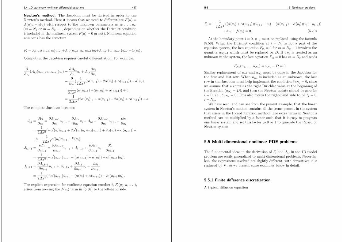
5.4 1D stationary nonlinear differential equations 457
Newton’s method. The Jacobian must be derived in order to useNewton’s method. Here it means that we need to differentiate F (u) =A(u)u − b(u) with respect to the unknown parameters u0, u1, . . . , um(m = Nx or m = Nx − 1, depending on whether the Dirichlet conditionis included in the nonlinear system F (u) = 0 or not). Nonlinear equationnumber i has the structure
Fi = Ai,i−1(ui−1, ui)ui−1+Ai,i(ui−1, ui, ui+1)ui+Ai,i+1(ui, ui+1)ui+1−bi(ui) .
Computing the Jacobian requires careful differentiation. For example,
∂
∂ui(Ai,i(ui−1, ui, ui+1)ui) = ∂Ai,i
∂uiui + Ai,i
∂ui∂ui
= ∂
∂ui( 12∆x2 (α(ui−1) + 2α(ui) + α(ui+1)) + a)ui+
12∆x2 (α(ui−1) + 2α(ui) + α(ui+1)) + a
= 12∆x2 (2α′(ui)ui + α(ui−1) + 2α(ui) + α(ui+1)) + a .
The complete Jacobian becomes
Ji,i = ∂Fi∂ui
= ∂Ai,i−1∂ui
ui−1 + ∂Ai,i∂ui
ui + Ai,i + ∂Ai,i+1∂ui
ui+1 −∂bi∂ui
= 12∆x2 (−α′(ui)ui−1 + 2α′(ui)ui + α(ui−1) + 2α(ui) + α(ui+1))+
a− 12∆x2α
′(ui)ui+1 − b′(ui),
Ji,i−1 = ∂Fi∂ui−1
= ∂Ai,i−1∂ui−1
ui−1 + Ai−1,i + ∂Ai,i∂ui−1
ui −∂bi∂ui−1
= 12∆x2 (−α′(ui−1)ui−1 − (α(ui−1) + α(ui)) + α′(ui−1)ui),
Ji,i+1 = ∂Ai,i+1∂ui−1
ui+1 + Ai+1,i + ∂Ai,i∂ui+1
ui −∂bi∂ui+1
= 12∆x2 (−α′(ui+1)ui+1 − (α(ui) + α(ui+1)) + α′(ui+1)ui) .
The explicit expression for nonlinear equation number i, Fi(u0, u1, . . .),arises from moving the f(ui) term in (5.56) to the left-hand side:
458 5 Nonlinear problems
Fi = − 12∆x2 ((α(ui) + α(ui+1))(ui+1 − ui)− (α(ui−1) + α(ui))(ui − ui−1))
+ aui − f(ui) = 0 . (5.70)
At the boundary point i = 0, u−1 must be replaced using the formula(5.58). When the Dirichlet condition at i = Nx is not a part of theequation system, the last equation Fm = 0 for m = Nx − 1 involves thequantity uNx−1 which must be replaced by D. If uNx is treated as anunknown in the system, the last equation Fm = 0 has m = Nx and reads
FNx(u0, . . . , uNx) = uNx −D = 0 .
Similar replacement of u−1 and uNx must be done in the Jacobian forthe first and last row. When uNx is included as an unknown, the lastrow in the Jacobian must help implement the condition δuNx = 0, sincewe assume that u contains the right Dirichlet value at the beginning ofthe iteration (uNx = D), and then the Newton update should be zero fori = 0, i.e., δuNx = 0. This also forces the right-hand side to be bi = 0,i = Nx.
We have seen, and can see from the present example, that the linearsystem in Newton’s method contains all the terms present in the systemthat arises in the Picard iteration method. The extra terms in Newton’smethod can be multiplied by a factor such that it is easy to programone linear system and set this factor to 0 or 1 to generate the Picard orNewton system.
5.5 Multi-dimensional nonlinear PDE problems
The fundamental ideas in the derivation of Fi and Ji,j in the 1D modelproblem are easily generalized to multi-dimensional problems. Neverthe-less, the expressions involved are slightly different, with derivatives in xreplaced by ∇, so we present some examples below in detail.
5.5.1 Finite difference discretization
A typical diffusion equation
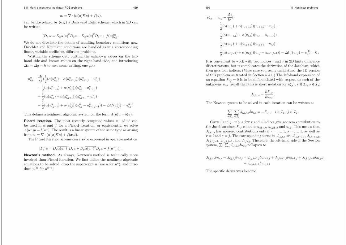
5.5 Multi-dimensional nonlinear PDE problems 459
ut = ∇ · (α(u)∇u) + f(u),
can be discretized by (e.g.) a Backward Euler scheme, which in 2D canbe written
[D−t u = Dxα(u)xDxu+Dyα(u)yDyu+ f(u)]ni,j .
We do not dive into the details of handling boundary conditions now.Dirichlet and Neumann conditions are handled as in a correspondinglinear, variable-coefficient diffusion problems.
Writing the scheme out, putting the unknown values on the left-hand side and known values on the right-hand side, and introducing∆x = ∆y = h to save some writing, one gets
uni,j −∆t
h2 (12(α(uni,j) + α(uni+1,j))(uni+1,j − uni,j)
− 12(α(uni−1,j) + α(uni,j))(uni,j − uni−1,j)
+ 12(α(uni,j) + α(uni,j+1))(uni,j+1 − uni,j)
− 12(α(uni,j−1) + α(uni,j))(uni,j − uni−1,j−1))−∆tf(uni,j) = un−1
i,j
This defines a nonlinear algebraic system on the form A(u)u = b(u).
Picard iteration. The most recently computed values u− of un canbe used in α and f for a Picard iteration, or equivalently, we solveA(u−)u = b(u−). The result is a linear system of the same type as arisingfrom ut = ∇ · (α(x)∇u) + f(x, t).
The Picard iteration scheme can also be expressed in operator notation:
[D−t u = Dxα(u−)xDxu+Dyα(u−)yDyu+ f(u−)]ni,j .
Newton’s method. As always, Newton’s method is technically moreinvolved than Picard iteration. We first define the nonlinear algebraicequations to be solved, drop the superscript n (use u for un), and intro-duce u(1) for un−1:
460 5 Nonlinear problems
Fi,j = ui,j −∆t
h2 (12(α(ui,j) + α(ui+1,j))(ui+1,j − ui,j)−12(α(ui−1,j) + α(ui,j))(ui,j − ui−1,j)+12(α(ui,j) + α(ui,j+1))(ui,j+1 − ui,j)−12(α(ui,j−1) + α(ui,j))(ui,j − ui−1,j−1))−∆t f(ui,j)− u(1)
i,j = 0 .
It is convenient to work with two indices i and j in 2D finite differencediscretizations, but it complicates the derivation of the Jacobian, whichthen gets four indices. (Make sure you really understand the 1D versionof this problem as treated in Section 5.4.1.) The left-hand expression ofan equation Fi,j = 0 is to be differentiated with respect to each of theunknowns ur,s (recall that this is short notation for unr,s), r ∈ Ix, s ∈ Iy:
Ji,j,r,s = ∂Fi,j∂ur,s
.
The Newton system to be solved in each iteration can be written as∑
r∈Ix
∑
s∈IyJi,j,r,sδur,s = −Fi,j , i ∈ Ix, j ∈ Iy .
Given i and j, only a few r and s indices give nonzero contribution tothe Jacobian since Fi,j contains ui±1,j , ui,j±1, and ui,j . This means thatJi,j,r,s has nonzero contributions only if r = i± 1, s = j ± 1, as well asr = i and s = j. The corresponding terms in Ji,j,r,s are Ji,j,i−1,j , Ji,j,i+1,j ,Ji,j,i,j−1, Ji,j,i,j+1, and Ji,j,i,j . Therefore, the left-hand side of the Newtonsystem,
∑r
∑s Ji,j,r,sδur,s collapses to
Ji,j,r,sδur,s = Ji,j,i,jδui,j + Ji,j,i−1,jδui−1,j + Ji,j,i+1,jδui+1,j + Ji,j,i,j−1δui,j−1
+ Ji,j,i,j+1δui,j+1
The specific derivatives become
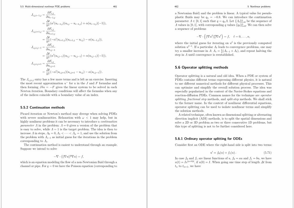
5.5 Multi-dimensional nonlinear PDE problems 461
Ji,j,i−1,j = ∂Fi,j∂ui−1,j
= ∆t
h2 (α′(ui−1,j)(ui,j − ui−1,j) + α(ui−1,j)(−1)),
Ji,j,i+1,j = ∂Fi,j∂ui+1,j
= ∆t
h2 (−α′(ui+1,j)(ui+1,j − ui,j)− α(ui−1,j)),
Ji,j,i,j−1 = ∂Fi,j∂ui,j−1
= ∆t
h2 (α′(ui,j−1)(ui,j − ui,j−1) + α(ui,j−1)(−1)),
Ji,j,i,j+1 = ∂Fi,j∂ui,j+1
= ∆t
h2 (−α′(ui,j+1)(ui,j+1 − ui,j)− α(ui,j−1)) .
The Ji,j,i,j entry has a few more terms and is left as an exercise. Insertingthe most recent approximation u− for u in the J and F formulas andthen forming Jδu = −F gives the linear system to be solved in eachNewton iteration. Boundary conditions will affect the formulas when anyof the indices coincide with a boundary value of an index.
5.5.2 Continuation methods
Picard iteration or Newton’s method may diverge when solving PDEswith severe nonlinearities. Relaxation with ω < 1 may help, but inhighly nonlinear problems it can be necessary to introduce a continuationparameter Λ in the problem: Λ = 0 gives a version of the problem thatis easy to solve, while Λ = 1 is the target problem. The idea is then toincrease Λ in steps, Λ0 = 0, Λ1 < · · · < Λn = 1, and use the solution fromthe problem with Λi−1 as initial guess for the iterations in the problemcorresponding to Λi.
The continuation method is easiest to understand through an example.Suppose we intend to solve
−∇ · (||∇u||q∇u) = f,
which is an equation modeling the flow of a non-Newtonian fluid through achannel or pipe. For q = 0 we have the Poisson equation (corresponding to
462 5 Nonlinear problems
a Newtonian fluid) and the problem is linear. A typical value for pseudo-plastic fluids may be qn = −0.8. We can introduce the continuationparameter Λ ∈ [0, 1] such that q = qnΛ. Let Λ`n`=0 be the sequence ofΛ values in [0, 1], with corresponding q values q`n`=0. We can then solvea sequence of problems
−∇ ·(||∇u`||q`∇u`
)= f, ` = 0, . . . , n,
where the initial guess for iterating on u` is the previously computedsolution u`−1. If a particular Λ` leads to convergence problems, one maytry a smaller increase in Λ: Λ∗ = 1
2(Λ`−1 + Λ`), and repeat halving thestep in Λ until convergence is reestablished.
5.6 Operator splitting methods
Operator splitting is a natural and old idea. When a PDE or system ofPDEs contains different terms expressing different physics, it is naturalto use different numerical methods for different physical processes. Thiscan optimize and simplify the overall solution process. The idea wasespecially popularized in the context of the Navier-Stokes equations andreaction-diffusion PDEs. Common names for the technique are operatorsplitting, fractional step methods, and split-step methods. We shall stickto the former name. In the context of nonlinear differential equations,operator splitting can be used to isolate nonlinear terms and simplifythe solution methods.
A related technique, often known as dimensional splitting or alternatingdirection implicit (ADI) methods, is to split the spatial dimensions andsolve a 2D or 3D problem as two or three consecutive 1D problems, butthis type of splitting is not to be further considered here.
5.6.1 Ordinary operator splitting for ODEsConsider first an ODE where the right-hand side is split into two terms:
u′ = f0(u) + f1(u) . (5.71)
In case f0 and f1 are linear functions of u, f0 = au and f1 = bu, we haveu(t) = Ie(a+b)t, if u(0) = I. When going one time step of length ∆t fromtn to tn+1, we have
5.6 Operator splitting methods 463
u(tn+1) = u(tn)e(a+b)∆t .
This expression can be also be written as
u(tn+1) = u(tn)ea∆teb∆t,
or
u∗ = u(tn)ea∆t, (5.72)u(tn+1) = u∗eb∆t (5.73)
The first step (5.72) means solving u′ = f0 over a time interval ∆t withu(tn) as start value. The second step (5.73) means solving u′ = f1 overa time interval ∆t with the value at the end of the first step as startvalue. That is, we progress the solution in two steps and solve two ODEsu′ = f0 and u′ = f1. The order of the equations is not important. Fromthe derivation above we see that solving u′ = f1 prior to u′ = f0 canequally well be done.
The technique is exact if the ODEs are linear. For nonlinear ODEsit is only an approximate method with error ∆t. The technique can beextended to an arbitrary number of steps; i.e., we may split the PDEsystem into any number of subsystems. Examples will illuminate thisprinciple.
5.6.2 Strang splitting for ODEs
The accuracy of the splitting method in Section 5.6.1 can be improvedfrom O(∆t) to O(∆t2) using so-called Strang splitting, where we takehalf a step with the f0 operator, a full step with the f1 operator, andfinally half another step with the f0 operator. During a time interval ∆tthe algorithm can be written as follows.
du∗
dt= f0(u∗), u∗(tn) = u(tn), t ∈ [tn, tn + 1
2∆t],du∗∗∗
dt= f1(u∗∗∗), u∗∗∗(tn) = u∗(tn+ 1
2), t ∈ [tn, tn +∆t],
du∗∗
dt= f0(u∗∗), u∗∗(tn+ 1
2) = u∗∗∗(tn+1), t ∈ [tn + 1
2∆t, tn +∆t] .
464 5 Nonlinear problems
The global solution is set as u(tn+1) = u∗∗(tn+1).There is no use in combining higher-order methods with ordinary
splitting since the error due to splitting is O(∆t), but for Strang splittingit makes sense to use schemes of order O(∆t2).
With the notation introduced for Strang splitting, we may expressordinary first-order splitting as
du∗
dt= f0(u∗), u∗(tn) = u(tn), t ∈ [tn, tn +∆t],
du∗∗
dt= f1(u∗∗), u∗∗(tn) = u∗(tn+1), t ∈ [tn, tn +∆t],
with global solution set as u(tn+1) = u∗∗(tn+1).
5.6.3 Example: Logistic growthLet us split the (scaled) logistic equation
u′ = u(1− u), u(0) = 0.1,
with solution u = (9e−t + 1)−1, into
u′ = u− u2 = f0(u) + f1(u), f0(u) = u, f1(u) = −u2 .
We solve u′ = f0(u) and u′ = f1(u) by a Forward Euler step. In addition,we add a method where we solve u′ = f0(u) analytically, since the equa-tion is actually u′ = u with solution et. The software that accompaniesthe following methods is the file split_logistic.py.
Splitting techniques. Ordinary splitting takes a Forward Euler step foreach of the ODEs according to
u∗,n+1 − u∗,n∆t
= f0(u∗,n), u∗,n = u(tn), t ∈ [tn, tn +∆t], (5.74)
u∗∗,n+1 − u∗∗,n∆t
= f1(u∗∗,n), u∗∗,n = u∗,n+1, t ∈ [tn, tn +∆t],(5.75)
with u(tn+1) = u∗∗,n+1.Strang splitting takes the form
5.6 Operator splitting methods 465
u∗,n+ 12 − u∗,n
12∆t
= f0(u∗,n), u∗,n = u(tn), t ∈ [tn, tn + 12∆t],
(5.76)u∗∗∗,n+1 − u∗∗∗,n
∆t= f1(u∗∗∗,n), u∗∗∗,n = u∗,n+ 1
2 , t ∈ [tn, tn +∆t],(5.77)
u∗∗,n+1 − u∗∗,n+ 12
12∆t
= f0(u∗∗,n+ 12 ), u∗∗,n+ 1
2 = u∗∗∗,n+1, t ∈ [tn + 12∆t, tn +∆t] .
(5.78)
Verbose implementation. The following function computes four solu-tions arising from the Forward Euler method, ordinary splitting, Strangsplitting, as well as Strang splitting with exact treatment of u′ = f0(u):
import numpy as np
def solver(dt, T, f, f_0, f_1):"""Solve u’=f by the Forward Euler method and by ordinary andStrang splitting: f(u) = f_0(u) + f_1(u)."""Nt = int(round(T/float(dt)))t = np.linspace(0, Nt*dt, Nt+1)u_FE = np.zeros(len(t))u_split1 = np.zeros(len(t)) # 1st-order splittingu_split2 = np.zeros(len(t)) # 2nd-order splittingu_split3 = np.zeros(len(t)) # 2nd-order splitting w/exact f_0
# Set initial valuesu_FE[0] = 0.1u_split1[0] = 0.1u_split2[0] = 0.1u_split3[0] = 0.1
for n in range(len(t)-1):# Forward Euler methodu_FE[n+1] = u_FE[n] + dt*f(u_FE[n])
# --- Ordinary splitting ---# First stepu_s_n = u_split1[n]u_s = u_s_n + dt*f_0(u_s_n)# Second stepu_ss_n = u_su_ss = u_ss_n + dt*f_1(u_ss_n)u_split1[n+1] = u_ss
466 5 Nonlinear problems
# --- Strang splitting ---# First stepu_s_n = u_split2[n]u_s = u_s_n + dt/2.*f_0(u_s_n)# Second stepu_sss_n = u_su_sss = u_sss_n + dt*f_1(u_sss_n)# Third stepu_ss_n = u_sssu_ss = u_ss_n + dt/2.*f_0(u_ss_n)u_split2[n+1] = u_ss
# --- Strang splitting using exact integrator for u’=f_0 ---# First stepu_s_n = u_split3[n]u_s = u_s_n*np.exp(dt/2.) # exact# Second stepu_sss_n = u_su_sss = u_sss_n + dt*f_1(u_sss_n)# Third stepu_ss_n = u_sssu_ss = u_ss_n*np.exp(dt/2.) # exactu_split3[n+1] = u_ss
return u_FE, u_split1, u_split2, u_split3, t
Compact implementation. We have used quite many lines for the stepsin the splitting methods. Many will prefer to condense the code a bit, asdone here:
# Ordinary splittingu_s = u_split1[n] + dt*f_0(u_split1[n])u_split1[n+1] = u_s + dt*f_1(u_s)
# Strang splittingu_s = u_split2[n] + dt/2.*f_0(u_split2[n])u_sss = u_s + dt*f_1(u_s)u_split2[n+1] = u_sss + dt/2.*f_0(u_sss)
# Strang splitting using exact integrator for u’=f_0u_s = u_split3[n]*np.exp(dt/2.) # exactu_ss = u_s + dt*f_1(u_s)u_split3[n+1] = u_ss*np.exp(dt/2.)
Results. Figure 5.3 shows that the impact of splitting is significant.Interestingly, however, the Forward Euler method applied to the entireproblem directly is much more accurate than any of the splitting schemes.We also see that Strang splitting is definitely more accurate than ordinarysplitting and that it helps a bit to use an exact solution of u′ = f0(u).With a large time step (∆t = 0.2, left plot in Figure 5.3), the asymptotic
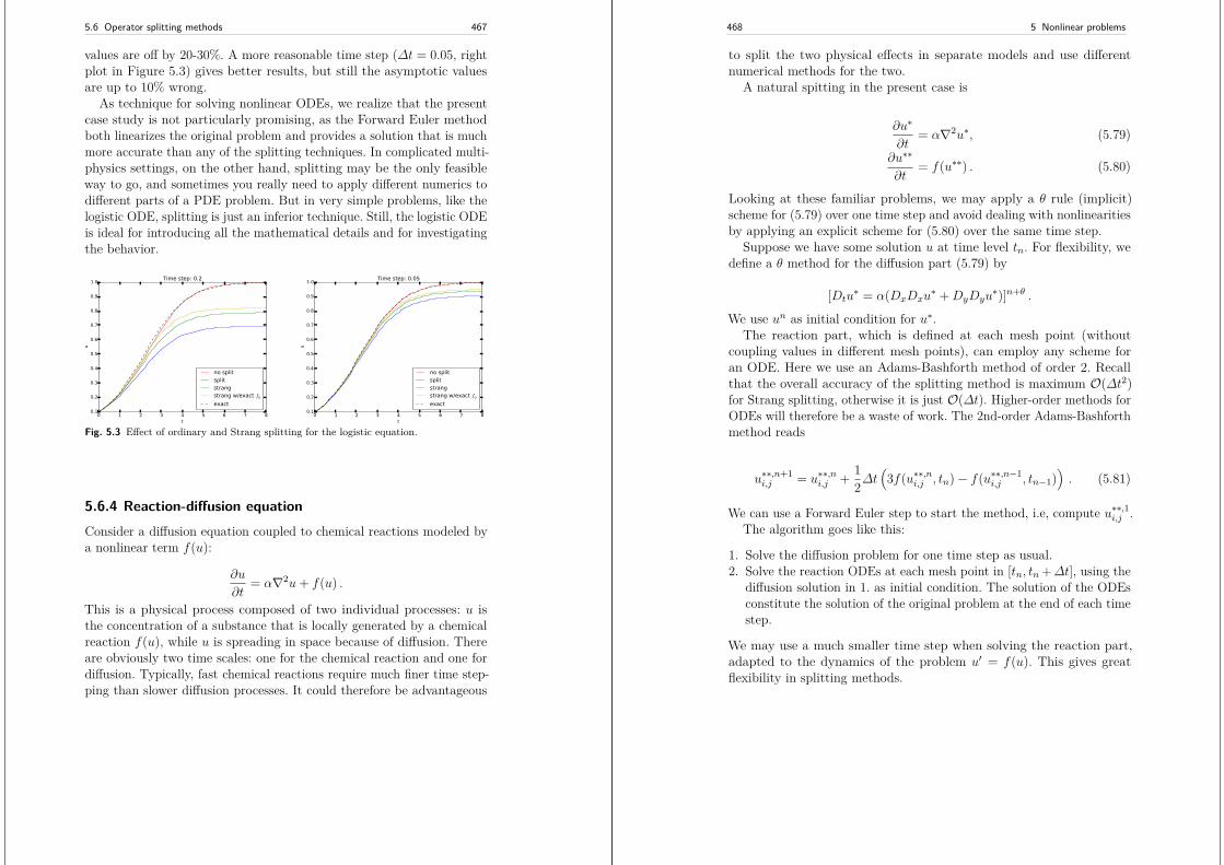
5.6 Operator splitting methods 467
values are off by 20-30%. A more reasonable time step (∆t = 0.05, rightplot in Figure 5.3) gives better results, but still the asymptotic valuesare up to 10% wrong.
As technique for solving nonlinear ODEs, we realize that the presentcase study is not particularly promising, as the Forward Euler methodboth linearizes the original problem and provides a solution that is muchmore accurate than any of the splitting techniques. In complicated multi-physics settings, on the other hand, splitting may be the only feasibleway to go, and sometimes you really need to apply different numerics todifferent parts of a PDE problem. But in very simple problems, like thelogistic ODE, splitting is just an inferior technique. Still, the logistic ODEis ideal for introducing all the mathematical details and for investigatingthe behavior.
0 1 2 3 4 5 6 7 8t
0.1
0.2
0.3
0.4
0.5
0.6
0.7
0.8
0.9
1.0
u
Time step: 0.2
no splitsplitstrangstrang w/exact f0
exact
0 1 2 3 4 5 6 7 8t
0.1
0.2
0.3
0.4
0.5
0.6
0.7
0.8
0.9
1.0
u
Time step: 0.05
no splitsplitstrangstrang w/exact f0
exact
Fig. 5.3 Effect of ordinary and Strang splitting for the logistic equation.
5.6.4 Reaction-diffusion equationConsider a diffusion equation coupled to chemical reactions modeled bya nonlinear term f(u):
∂u
∂t= α∇2u+ f(u) .
This is a physical process composed of two individual processes: u isthe concentration of a substance that is locally generated by a chemicalreaction f(u), while u is spreading in space because of diffusion. Thereare obviously two time scales: one for the chemical reaction and one fordiffusion. Typically, fast chemical reactions require much finer time step-ping than slower diffusion processes. It could therefore be advantageous
468 5 Nonlinear problems
to split the two physical effects in separate models and use differentnumerical methods for the two.
A natural spitting in the present case is
∂u∗
∂t= α∇2u∗, (5.79)
∂u∗∗
∂t= f(u∗∗) . (5.80)
Looking at these familiar problems, we may apply a θ rule (implicit)scheme for (5.79) over one time step and avoid dealing with nonlinearitiesby applying an explicit scheme for (5.80) over the same time step.
Suppose we have some solution u at time level tn. For flexibility, wedefine a θ method for the diffusion part (5.79) by
[Dtu∗ = α(DxDxu
∗ +DyDyu∗)]n+θ .
We use un as initial condition for u∗.The reaction part, which is defined at each mesh point (without
coupling values in different mesh points), can employ any scheme foran ODE. Here we use an Adams-Bashforth method of order 2. Recallthat the overall accuracy of the splitting method is maximum O(∆t2)for Strang splitting, otherwise it is just O(∆t). Higher-order methods forODEs will therefore be a waste of work. The 2nd-order Adams-Bashforthmethod reads
u∗∗,n+1i,j = u∗∗,ni,j + 1
2∆t(3f(u∗∗,ni,j , tn)− f(u∗∗,n−1
i,j , tn−1)). (5.81)
We can use a Forward Euler step to start the method, i.e, compute u∗∗,1i,j .The algorithm goes like this:
1. Solve the diffusion problem for one time step as usual.2. Solve the reaction ODEs at each mesh point in [tn, tn +∆t], using the
diffusion solution in 1. as initial condition. The solution of the ODEsconstitute the solution of the original problem at the end of each timestep.
We may use a much smaller time step when solving the reaction part,adapted to the dynamics of the problem u′ = f(u). This gives greatflexibility in splitting methods.
5.6 Operator splitting methods 469
5.6.5 Example: Reaction-Diffusion with linear reaction term
The methods above may be explored in detail through a specific compu-tational example in which we compute the convergence rates associatedwith four different solution approaches for the reaction-diffusion equationwith a linear reaction term, i.e. f(u) = −bu. The methods comprisesolving without splitting (just straight Forward Euler), ordinary splitting,first order Strang splitting, and second order Strang splitting. In all fourmethods, a standard centered difference approximation is used for thespatial second derivative. The methods share the error model E = Chr,while differing in the step h (being either dx2 or dx) and the convergencerate r (being either 1 or 2).
All code commented below is found in the file split_diffu_react.py.When executed, a function convergence_rates is called, from which allconvergence rate computations are handled:
def convergence_rates(scheme=’diffusion’):
F = 0.5 # Upper limit for FE (stability). For CN, this# limit does not apply, but for simplicity, we# choose F = 0.5 as the initial F value.
T = 1.2a = 3.5b = 1L = 1.5k = np.pi/L
def exact(x, t):’’’exact sol. to: du/dt = a*d^2u/dx^2 - b*u’’’return np.exp(-(a*k**2 + b)*t) * np.sin(k*x)
def f(u, t):return -b*u
def I(x):return exact(x, 0)
global error # error computed in the user action functionerror = 0
# Convergence studydef action(u, x, t, n):
global errorif n == 1: # New simulation, - reset error
error = 0else:
error = max(error, np.abs(u - exact(x, t[n])).max())
E = []
470 5 Nonlinear problems
h = []Nx_values = [10, 20, 40, 80] # i.e., dx halved each timefor Nx in Nx_values:
dx = L/Nxif scheme == ’Strang_splitting_2ndOrder’:
print ’Strang splitting with 2nd order schemes...’# In this case, E = C*h**r (with r = 2) and since# h = dx = K*dt, the ratio dt/dx must be constant.# To fulfill this demand, we must let F change# when dx changes. From F = a*dt/dx**2, it follows# that halving dx AND doubling F assures dt/dx const.# Initially, we simply choose F = 0.5.
dt = F/a*dx**2#print ’dt/dx:’, dt/dxNt = int(round(T/float(dt)))t = np.linspace(0, Nt*dt, Nt+1) # global timeStrang_splitting_2ndOrder(I=I, a=a, b=b, f=f, L=L, dt=dt,
dt_Rfactor=1, F=F, t=t, T=T,user_action=action)
h.append(dx)# prepare for next iteration (make F match dx/2)F = F*2 # assures dt/dx const. when dx = dx/2
else:# In these cases, E = C*h**r (with r = 1) and since# h = dx**2 = K*dt, the ratio dt/dx**2 must be constant.# This is fulfilled by choosing F = 0.5 (for FE stability)# and make sure that F, dx and dt comply to F = a*dt/dx**2.dt = F/a*dx**2Nt = int(round(T/float(dt)))t = np.linspace(0, Nt*dt, Nt+1) # global timeif scheme == ’diffusion’:
print ’FE on whole eqn...’diffusion_theta(I, a, f, L, dt, F, t, T,
step_no=0, theta=0,u_L=0, u_R=0, user_action=action)
h.append(dx**2)elif scheme == ’ordinary_splitting’:
print ’Ordinary splitting...’ordinary_splitting(I=I, a=a, b=b, f=f, L=L, dt=dt,
dt_Rfactor=1, F=F, t=t, T=T,user_action=action)
h.append(dx**2)elif scheme == ’Strang_splitting_1stOrder’:
print ’Strang splitting with 1st order schemes...’Strang_splitting_1stOrder(I=I, a=a, b=b, f=f, L=L, dt=dt,
dt_Rfactor=1, F=F, t=t, T=T,user_action=action)
h.append(dx**2)else:
print ’Unknown scheme requested!’sys.exit(0)
#print ’dt/dx**2:’, dt/dx**2
5.6 Operator splitting methods 471
E.append(error)Nx *= 2 # Nx doubled gives dx/2
print ’E:’, Eprint ’h:’, h
# Convergence ratesr = [np.log(E[i]/E[i-1])/np.log(h[i]/h[i-1])
for i in range(1,len(Nx_values))]print ’Computed rates:’, r
if __name__ == ’__main__’:
schemes = [’diffusion’,’ordinary_splitting’,’Strang_splitting_1stOrder’,’Strang_splitting_2ndOrder’]
for scheme in schemes:convergence_rates(scheme=scheme)
Now, with respect to the error (E = Chr), the Forward Euler scheme,the ordinary splitting scheme and first order Strang splitting schemeare all first order (r = 1), with a step h = ∆x2 = K−1∆t, where K issome constant. This implies that the ratio ∆t
∆x2 must be held constantduring convergence rate calculations. Furthermore, the Fourier numberF = α∆t
∆x2 is upwards limited to F = 0.5, being the stability limit withexplicit schemes. Thus, in these cases, we use the fixed value of F and agiven (but changing) spatial resolution ∆x to compute the correspondingvalue of ∆t according to the expression for F . This assures that ∆t
∆x2 iskept constant. The loop in convergence_rates runs over a chosen setof grid points (Nx_values) which gives a doubling of spatial resolutionwith each iteration (∆x is halved).
For the second order Strang splitting scheme, we have r = 2 and astep h = ∆x = K−1∆t, where K again is some constant. In this case, itis thus the ratio ∆t
∆x that must be held constant during the convergencerate calculations. From the expression for F , it is clear then that Fmust change with each halving of ∆x. In fact, if F is doubled each time∆x is halved, the ratio ∆t
∆x will be constant (this follows, e.g., from theexpression for F ). This us utilized in our code.
A solver diffusion_theta is used in each of the four solution ap-proaches:
def diffusion_theta(I, a, f, L, dt, F, t, T, step_no, theta=0.5,u_L=0, u_R=0, user_action=None):
472 5 Nonlinear problems
"""Full solver for the model problem using the theta-ruledifference approximation in time (no restriction on F,i.e., the time step when theta >= 0.5). Vectorizedimplementation and sparse (tridiagonal) coefficient matrix.Note that t always covers the whole global time interval, whethersplitting is the case or not. T, on the other hand, isthe end of the global time interval if there is no split,but if splitting, we use T=dt. When splitting, step_nokeeps track of the time step number (for lookup in t)."""
Nt = int(round(T/float(dt)))dx = np.sqrt(a*dt/F)Nx = int(round(L/dx))x = np.linspace(0, L, Nx+1) # Mesh points in space# Make sure dx and dt are compatible with x and tdx = x[1] - x[0]dt = t[1] - t[0]
u = np.zeros(Nx+1) # solution array at t[n+1]u_1 = np.zeros(Nx+1) # solution at t[n]
# Representation of sparse matrix and right-hand sidediagonal = np.zeros(Nx+1)lower = np.zeros(Nx)upper = np.zeros(Nx)b = np.zeros(Nx+1)
# Precompute sparse matrix (scipy format)Fl = F*thetaFr = F*(1-theta)diagonal[:] = 1 + 2*Fllower[:] = -Fl #1upper[:] = -Fl #1# Insert boundary conditionsdiagonal[0] = 1upper[0] = 0diagonal[Nx] = 1lower[-1] = 0
diags = [0, -1, 1]A = scipy.sparse.diags(
diagonals=[diagonal, lower, upper],offsets=[0, -1, 1], shape=(Nx+1, Nx+1),format=’csr’)
#print A.todense()
# Allow f to be None or 0if f is None or f == 0:
f = lambda x, t: np.zeros((x.size)) \if isinstance(x, np.ndarray) else 0
# Set initial condition
5.6 Operator splitting methods 473
if isinstance(I, np.ndarray): # I is an arrayu_1 = np.copy(I)
else: # I is a functionfor i in range(0, Nx+1):
u_1[i] = I(x[i])
if user_action is not None:user_action(u_1, x, t, step_no+0)
# Time loopfor n in range(0, Nt):
b[1:-1] = u_1[1:-1] + \Fr*(u_1[:-2] - 2*u_1[1:-1] + u_1[2:]) + \dt*theta*f(u_1[1:-1], t[step_no+n+1]) + \dt*(1-theta)*f(u_1[1:-1], t[step_no+n])
b[0] = u_L; b[-1] = u_R # boundary conditionsu[:] = scipy.sparse.linalg.spsolve(A, b)
if user_action is not None:user_action(u, x, t, step_no+(n+1))
# Update u_1 before next stepu_1, u = u, u_1
# u is now contained in u_1 (swapping)return u_1
For the no splitting approach with Forward Euler in time, thissolver handles both the diffusion and the reaction term. When splitting,diffusion_theta takes care of the diffusion term only, while the reactionterm is handled either by a Forward Euler scheme in reaction_FE, or bya second order Adams-Bashforth scheme from Odespy. The reaction_FEfunction covers one complete time step dt during ordinary splitting, whileStrang splitting (both first and second order) applies it with dt/2 twiceduring each time step dt. Since the reaction term typically represents amuch faster process than the diffusion term, a further refinement of thetime step is made possible in reaction_FE. It was implemented as
def reaction_FE(I, f, L, Nx, dt, dt_Rfactor, t, step_no,user_action=None):
"""Reaction solver, Forward Euler method.Note the at t covers the whole global time interval.dt is either one complete,or one half, of the step in thediffusion part, i.e. there is a local time interval[0, dt] or [0, dt/2] that the reaction_FEdeals with each time it is called. step_no keepstrack of the (global) time step number (requiredfor lookup in t)."""
u = np.copy(I)
474 5 Nonlinear problems
dt_local = dt/float(dt_Rfactor)Nt_local = int(round(dt/float(dt_local)))x = np.linspace(0, L, Nx+1)
for n in range(Nt_local):time = t[step_no] + n*dt_localu[1:Nx] = u[1:Nx] + dt_local*f(u[1:Nx], time)
# BC already inserted in diffusion step, i.e. no action herereturn u
With the ordinary splitting approach, each time step dt is covered twice.First computing the impact of the reaction term, then the contributionfrom the diffusion term:
def ordinary_splitting(I, a, b, f, L, dt,dt_Rfactor, F, t, T,user_action=None):
’’’1st order scheme, i.e. Forward Euler is enough for boththe diffusion and the reaction part. The time step dt isgiven for the diffusion step, while the time step for thereaction part is found as dt/dt_Rfactor, where dt_Rfactor >= 1.’’’Nt = int(round(T/float(dt)))dx = np.sqrt(a*dt/F)Nx = int(round(L/dx))x = np.linspace(0, L, Nx+1) # Mesh points in spaceu = np.zeros(Nx+1)
# Set initial condition u(x,0) = I(x)for i in range(0, Nx+1):
u[i] = I(x[i])
# In the following loop, each time step is "covered twice",# first for reaction, then for diffusionfor n in range(0, Nt):
# Reaction step (potentially many smaller steps within dt)u_s = reaction_FE(I=u, f=f, L=L, Nx=Nx,
dt=dt, dt_Rfactor=dt_Rfactor,t=t, step_no=n,user_action=None)
u = diffusion_theta(I=u_s, a=a, f=0, L=L, dt=dt, F=F,t=t, T=dt, step_no=n, theta=0,u_L=0, u_R=0, user_action=None)
if user_action is not None:user_action(u, x, t, n+1)
return
For the two Strang splitting approaches, each time step dt is handledby first computing the reaction step for (the first) dt/2, followed by
5.6 Operator splitting methods 475
a diffusion step dt, before the reaction step is treated once again for(the remaining) dt/2. Since first order Strang splitting is no better thanfirst order accurate, both the reaction and diffusion steps are computedexplicitly. The solver was implemented as
def Strang_splitting_1stOrder(I, a, b, f, L, dt, dt_Rfactor,F, t, T, user_action=None):
’’’Strang splitting while still using FE for the reactionstep and for the diffusion step. Gives 1st order scheme.The time step dt is given for the diffusion step, whilethe time step for the reaction part is found as0.5*dt/dt_Rfactor, where dt_Rfactor >= 1. Introduce anextra time mesh t2 for the reaction part, since it steps dt/2.’’’Nt = int(round(T/float(dt)))t2 = np.linspace(0, Nt*dt, (Nt+1)+Nt) # Mesh points in diffdx = np.sqrt(a*dt/F)Nx = int(round(L/dx))x = np.linspace(0, L, Nx+1)u = np.zeros(Nx+1)
# Set initial condition u(x,0) = I(x)for i in range(0, Nx+1):
u[i] = I(x[i])
for n in range(0, Nt):# Reaction step (1/2 dt: from t_n to t_n+1/2)# (potentially many smaller steps within dt/2)u_s = reaction_FE(I=u, f=f, L=L, Nx=Nx,
dt=dt/2.0, dt_Rfactor=dt_Rfactor,t=t2, step_no=2*n,user_action=None)
# Diffusion step (1 dt: from t_n to t_n+1)u_sss = diffusion_theta(I=u_s, a=a, f=0, L=L, dt=dt, F=F,
t=t, T=dt, step_no=n, theta=0,u_L=0, u_R=0, user_action=None)
# Reaction step (1/2 dt: from t_n+1/2 to t_n+1)# (potentially many smaller steps within dt/2)u = reaction_FE(I=u_sss, f=f, L=L, Nx=Nx,
dt=dt/2.0, dt_Rfactor=dt_Rfactor,t=t2, step_no=2*n+1,user_action=None)
if user_action is not None:user_action(u, x, t, n+1)
return
The second order version of the Strang splitting approach utilizes asecond order Adams-Bashforth solver for the reaction part and a Crank-Nicolson scheme for the diffusion part. The solver has the same structureas the one for first order Strang splitting and was implemented as
476 5 Nonlinear problems
def Strang_splitting_2ndOrder(I, a, b, f, L, dt, dt_Rfactor,F, t, T, user_action=None):
’’’Strang splitting using Crank-Nicolson for the diffusionstep (theta-rule) and Adams-Bashforth 2 for the reaction step.Gives 2nd order scheme. Introduce an extra time mesh t2 forthe reaction part, since it steps dt/2.’’’import odespyNt = int(round(T/float(dt)))t2 = np.linspace(0, Nt*dt, (Nt+1)+Nt) # Mesh points in diffdx = np.sqrt(a*dt/F)Nx = int(round(L/dx))x = np.linspace(0, L, Nx+1)u = np.zeros(Nx+1)
# Set initial condition u(x,0) = I(x)for i in range(0, Nx+1):
u[i] = I(x[i])
reaction_solver = odespy.AdamsBashforth2(f)
for n in range(0, Nt):# Reaction step (1/2 dt: from t_n to t_n+1/2)# (potentially many smaller steps within dt/2)reaction_solver.set_initial_condition(u)t_points = np.linspace(0, dt/2.0, dt_Rfactor+1)u_AB2, t_ = reaction_solver.solve(t_points) # t_ not neededu_s = u_AB2[-1,:] # pick sol at last point in time
# Diffusion step (1 dt: from t_n to t_n+1)u_sss = diffusion_theta(I=u_s, a=a, f=0, L=L, dt=dt, F=F,
t=t, T=dt, step_no=n, theta=0.5,u_L=0, u_R=0, user_action=None)
# Reaction step (1/2 dt: from t_n+1/2 to t_n+1)# (potentially many smaller steps within dt/2)reaction_solver.set_initial_condition(u_sss)t_points = np.linspace(0, dt/2.0, dt_Rfactor+1)u_AB2, t_ = reaction_solver.solve(t_points) # t_ not neededu = u_AB2[-1,:] # pick sol at last point in time
if user_action is not None:user_action(u, x, t, n+1)
return
When executing split_diffu_react.py, we find that the estimatedconvergence rates are as expected. The second order Strang splitting givesthe least error (about 4e−5) and has second order convergence (r = 2),while the remaining three approaches have first order convergence (r = 1).
5.6 Operator splitting methods 477
5.6.6 Analysis of the splitting method
Let us address a linear PDE problem for which we can develop analyticalsolutions of the discrete equations, with and without splitting, and discussthese. Choosing f(u) = −βu for a constant β gives a linear problem. Weuse the Forward Euler method for both the PDE and ODE problems.
We seek a 1D Fourier wave component solution of the problem, as-suming homogeneous Dirichlet conditions at x = 0 and x = L:
u = e−αk2t−βt sin kx, k = π
L.
This component fits the 1D PDE problem (f = 0). On complex form wecan write
u = e−αk2t−βt+ikx,
where i =√−1 and the imaginary part is taken as the physical solution.
We refer to Section 3.3 and to the book [9] for a discussion of exactnumerical solutions to diffusion and decay problems, respectively. The keyidea is to search for solutions Aneikx and determine A. For the diffusionproblem solved by a Forward Euler method one has
A = 1− 4F sinp,
where F = α∆t/∆x2 is the mesh Fourier number and p = k∆x/2 is adimensionless number reflecting the spatial resolution (number of pointsper wave length in space). For the decay problem u′ = −βu, we haveA = 1− q, where q is a dimensionless parameter reflecting the resolutionin the decay problem: q = β∆t.
The original model problem can also be discretized by a Forward Eulerscheme,
[D+t u = αDxDxu− βu]ni .
Assuming Aneikx we find that
uni = (1− 4F sinp−q)n sin kx .
We are particularly interested in what happens at one time step. That is,
uni = (1− 4F sin2 p)un−1i .
In the two stage algorithm, we first compute the diffusion step
478 5 Nonlinear problems
u∗,n+1i = (1− 4F sin2 p)un−1
i .
Then we use this as input to the decay algorithm and arrive at
u∗∗,n+1 = (1− q)u∗,n+1 = (1− q)(1− 4F sin2 p)un−1i .
The splitting approximation over one step is therefore
E = 1− 4F sinp−q − (1− q)(1− 4F sin2 p) = −q(2− F sin2 p))
5.7 Exercises
Problem 5.1: Determine if equations are nonlinear or notClassify each term in the following equations as linear or nonlinear.Assume that u, u, and p are unknown functions and that all othersymbols are known quantities.
1. mu′′ + β|u′|u′ + cu = F (t)2. ut = αuxx3. utt = c2∇2u4. ut = ∇ · (α(u)∇u) + f(x, y)5. ut + f(u)x = 06. ut + u · ∇u = −∇p+ r∇2u, ∇ · u = 0 (u is a vector field)7. u′ = f(u, t)8. ∇2u = λeu
Filename: nonlinear_vs_linear.
Problem 5.2: Derive and investigate a generalized logisticmodelThe logistic model for population growth is derived by assuming anonlinear growth rate,
u′ = a(u)u, u(0) = I, (5.82)
and the logistic model arises from the simplest possible choice of a(u):r(u) = %(1 − u/M), where M is the maximum value of u that the
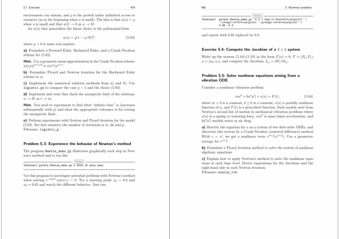
5.7 Exercises 479
environment can sustain, and % is the growth under unlimited access toresources (as in the beginning when u is small). The idea is that a(u) ∼ %when u is small and that a(t)→ 0 as u→M .
An a(u) that generalizes the linear choice is the polynomial form
a(u) = %(1− u/M)p, (5.83)
where p > 0 is some real number.
a) Formulate a Forward Euler, Backward Euler, and a Crank-Nicolsonscheme for (5.82).
Hint. Use a geometric mean approximation in the Crank-Nicolson scheme:[a(u)u]n+1/2 ≈ a(un)un+1.
b) Formulate Picard and Newton iteration for the Backward Eulerscheme in a).
c) Implement the numerical solution methods from a) and b). Uselogistic.py to compare the case p = 1 and the choice (5.83).
d) Implement unit tests that check the asymptotic limit of the solutions:u→M as t→∞.
Hint. You need to experiment to find what “infinite time” is (increasessubstantially with p) and what the appropriate tolerance is for testingthe asymptotic limit.
e) Perform experiments with Newton and Picard iteration for the model(5.83). See how sensitive the number of iterations is to ∆t and p.Filename: logistic_p.
Problem 5.3: Experience the behavior of Newton’s method
The program Newton_demo.py illustrates graphically each step in New-ton’s method and is run like
Terminal
Terminal> python Newton_demo.py f dfdx x0 xmin xmax
Use this program to investigate potential problems with Newton’s methodwhen solving e−0.5x2 cos(πx) = 0. Try a starting point x0 = 0.8 andx0 = 0.85 and watch the different behavior. Just run
480 5 Nonlinear problems
Terminal
Terminal> python Newton_demo.py ’0.2 + exp(-0.5*x**2)*cos(pi*x)’ \’-x*exp(-x**2)*cos(pi*x) - pi*exp(-x**2)*sin(pi*x)’ \0.85 -3 3
and repeat with 0.85 replaced by 0.8.
Exercise 5.4: Compute the Jacobian of a 2× 2 system
Write up the system (5.18)-(5.19) in the form F (u) = 0, F = (F0, F1),u = (u0, u1), and compute the Jacobian Ji,j = ∂Fi/∂uj .
Problem 5.5: Solve nonlinear equations arising from avibration ODE
Consider a nonlinear vibration problem
mu′′ + bu′|u′|+ s(u) = F (t), (5.84)
where m > 0 is a constant, b ≥ 0 is a constant, s(u) a possibly nonlinearfunction of u, and F (t) is a prescribed function. Such models arise fromNewton’s second law of motion in mechanical vibration problems wheres(u) is a spring or restoring force, mu′′ is mass times acceleration, andbu′|u′| models water or air drag.
a) Rewrite the equation for u as a system of two first-order ODEs, anddiscretize this system by a Crank-Nicolson (centered difference) method.With v = u′, we get a nonlinear term vn+ 1
2 |vn+ 12 |. Use a geometric
average for vn+ 12 .
b) Formulate a Picard iteration method to solve the system of nonlinearalgebraic equations.
c) Explain how to apply Newton’s method to solve the nonlinear equa-tions at each time level. Derive expressions for the Jacobian and theright-hand side in each Newton iteration.Filename: nonlin_vib.
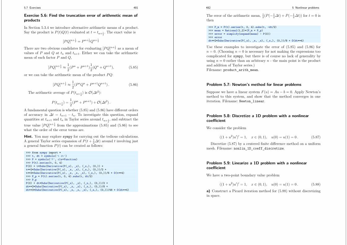
5.7 Exercises 481
Exercise 5.6: Find the truncation error of arithmetic mean ofproducts
In Section 5.3.4 we introduce alternative arithmetic means of a product.Say the product is P (t)Q(t) evaluated at t = tn+ 1
2. The exact value is
[PQ]n+ 12 = P n+ 1
2Qn+ 12
There are two obvious candidates for evaluating [PQ]n+ 12 as a mean of
values of P and Q at tn and tn+1. Either we can take the arithmeticmean of each factor P and Q,
[PQ]n+ 12 ≈ 1
2(P n + P n+1)12(Qn +Qn+1), (5.85)
or we can take the arithmetic mean of the product PQ:
[PQ]n+ 12 ≈ 1
2(P nQn + P n+1Qn+1) . (5.86)
The arithmetic average of P (tn+ 12) is O(∆t2):
P (tn+ 12) = 1
2(P n + P n+1) +O(∆t2) .
A fundamental question is whether (5.85) and (5.86) have different ordersof accuracy in ∆t = tn+1 − tn. To investigate this question, expandquantities at tn+1 and tn in Taylor series around tn+ 1
2, and subtract the
true value [PQ]n+ 12 from the approximations (5.85) and (5.86) to see
what the order of the error terms are.
Hint. You may explore sympy for carrying out the tedious calculations.A general Taylor series expansion of P (t+ 1
2∆t) around t involving justa general function P (t) can be created as follows:
>>> from sympy import *>>> t, dt = symbols(’t dt’)>>> P = symbols(’P’, cls=Function)>>> P(t).series(t, 0, 4)P(0) + t*Subs(Derivative(P(_x), _x), (_x,), (0,)) +t**2*Subs(Derivative(P(_x), _x, _x), (_x,), (0,))/2 +t**3*Subs(Derivative(P(_x), _x, _x, _x), (_x,), (0,))/6 + O(t**4)>>> P_p = P(t).series(t, 0, 4).subs(t, dt/2)>>> P_pP(0) + dt*Subs(Derivative(P(_x), _x), (_x,), (0,))/2 +dt**2*Subs(Derivative(P(_x), _x, _x), (_x,), (0,))/8 +dt**3*Subs(Derivative(P(_x), _x, _x, _x), (_x,), (0,))/48 + O(dt**4)
482 5 Nonlinear problems
The error of the arithmetic mean, 12(P (−1
2∆t) + P (−12∆t)) for t = 0 is
then
>>> P_m = P(t).series(t, 0, 4).subs(t, -dt/2)>>> mean = Rational(1,2)*(P_m + P_p)>>> error = simplify(expand(mean) - P(0))>>> errordt**2*Subs(Derivative(P(_x), _x, _x), (_x,), (0,))/8 + O(dt**4)
Use these examples to investigate the error of (5.85) and (5.86) forn = 0. (Choosing n = 0 is necessary for not making the expressions toocomplicated for sympy, but there is of course no lack of generality byusing n = 0 rather than an arbitrary n - the main point is the productand addition of Taylor series.)Filename: product_arith_mean.
Problem 5.7: Newton’s method for linear problemsSuppose we have a linear system F (u) = Au− b = 0. Apply Newton’smethod to this system, and show that the method converges in oneiteration. Filename: Newton_linear.
Problem 5.8: Discretize a 1D problem with a nonlinearcoefficientWe consider the problem
((1 + u2)u′)′ = 1, x ∈ (0, 1), u(0) = u(1) = 0 . (5.87)
Discretize (5.87) by a centered finite difference method on a uniformmesh. Filename: nonlin_1D_coeff_discretize.
Problem 5.9: Linearize a 1D problem with a nonlinearcoefficientWe have a two-point boundary value problem
((1 + u2)u′)′ = 1, x ∈ (0, 1), u(0) = u(1) = 0 . (5.88)
a) Construct a Picard iteration method for (5.88) without discretizingin space.
5.7 Exercises 483
b) Apply Newton’s method to (5.88) without discretizing in space.
c) Discretize (5.88) by a centered finite difference scheme. Construct aPicard method for the resulting system of nonlinear algebraic equations.
d) Discretize (5.88) by a centered finite difference scheme. Define thesystem of nonlinear algebraic equations, calculate the Jacobian, and setup Newton’s method for solving the system.Filename: nonlin_1D_coeff_linearize.
Problem 5.10: Finite differences for the 1D Bratu problem
We address the so-called Bratu problem
u′′ + λeu = 0, x ∈ (0, 1), u(0) = u(1) = 0, (5.89)
where λ is a given parameter and u is a function of x. This is a widely usedmodel problem for studying numerical methods for nonlinear differentialequations. The problem (5.89) has an exact solution
ue(x) = −2 ln(
cosh((x− 12)θ/2)
cosh(θ/4)
),
where θ solves
θ =√
2λ cosh(θ/4) .
There are two solutions of (5.89) for 0 < λ < λc and no solution forλ > λc. For λ = λc there is one unique solution. The critical value λcsolves
1 =√
2λc14 sinh(θ(λc)/4) .
A numerical value is λc = 3.513830719.
a) Discretize (5.89) by a centered finite difference method.
b) Set up the nonlinear equations Fi(u0, u1, . . . , uNx) = 0 from a). Cal-culate the associated Jacobian.
c) Implement a solver that can compute u(x) using Newton’s method.Plot the error as a function of x in each iteration.
484 5 Nonlinear problems
d) Investigate whether Newton’s method gives second-order convergenceby computing ||ue−u||/||ue−u−||2 in each iteration, where u is solutionin the current iteration and u− is the solution in the previous iteration.Filename: nonlin_1D_Bratu_fd.
Problem 5.11: Discretize a nonlinear 1D heat conductionPDE by finite differencesWe address the 1D heat conduction PDE
%c(T )Tt = (k(T )Tx)x,
for x ∈ [0, L], where % is the density of the solid material, c(T ) is theheat capacity, T is the temperature, and k(T ) is the heat conductioncoefficient. T (x, 0) = I(x), and ends are subject to a cooling law:
k(T )Tx|x=0 = h(T )(T − Ts), −k(T )Tx|x=L = h(T )(T − Ts),
where h(T ) is a heat transfer coefficient and Ts is the given surroundingtemperature.a) Discretize this PDE in time using either a Backward Euler or Crank-Nicolson scheme.b) Formulate a Picard iteration method for the time-discrete problem(i.e., an iteration method before discretizing in space).c) Formulate a Newton method for the time-discrete problem in b).d) Discretize the PDE by a finite difference method in space. Derive thematrix and right-hand side of a Picard iteration method applied to thespace-time discretized PDE.e) Derive the matrix and right-hand side of a Newton method appliedto the discretized PDE in d).Filename: nonlin_1D_heat_FD.
Problem 5.12: Differentiate a highly nonlinear termThe operator ∇· (α(u)∇u) with α(u) = |∇u|q appears in several physicalproblems, especially flow of Non-Newtonian fluids. The expression |∇u|is defined as the Euclidean norm of a vector: |∇u|2 = ∇u · ∇u. In a
5.7 Exercises 485
Newton method one has to carry out the differentiation ∂α(u)/∂cj , foru =
∑k ckψk. Show that
∂
∂uj|∇u|q = q|∇u|q−2∇u · ∇ψj .
Filename: nonlin_differentiate.
Exercise 5.13: Crank-Nicolson for a nonlinear 3D diffusionequationRedo Section 5.5.1 when a Crank-Nicolson scheme is used to discretizethe equations in time and the problem is formulated for three spatialdimensions.Hint. Express the Jacobian as Ji,j,k,r,s,t = ∂Fi,j,k/∂ur,s,t and observe,as in the 2D case, that Ji,j,k,r,s,t is very sparse: Ji,j,k,r,s,t 6= 0 only forr = i± i, s = j ± 1, and t = k ± 1 as well as r = i, s = j, and t = k.Filename: nonlin_heat_FD_CN_2D.
Problem 5.14: Find the sparsity of the JacobianConsider a typical nonlinear Laplace term like ∇ · α(u)∇u discretized bycentered finite differences. Explain why the Jacobian corresponding tothis term has the same sparsity pattern as the matrix associated withthe corresponding linear term α∇2u.Hint. Set up the unknowns that enter the difference equation at a point(i, j) in 2D or (i, j, k) in 3D, and identify the nonzero entries of theJacobian that can arise from such a type of difference equation.Filename: nonlin_sparsity_Jacobian.
Problem 5.15: Investigate a 1D problem with a continuationmethodFlow of a pseudo-plastic power-law fluid between two flat plates can bemodeled by
d
dx
(µ0
∣∣∣∣du
dx
∣∣∣∣n−1 du
dx
)= −β, u′(0) = 0, u(H) = 0,
486 5 Nonlinear problems
where β > 0 and µ0 > 0 are constants. A target value of n may ben = 0.2.
a) Formulate a Picard iteration method directly for the differentialequation problem.
b) Perform a finite difference discretization of the problem in each Picarditeration. Implement a solver that can compute u on a mesh. Verify thatthe solver gives an exact solution for n = 1 on a uniform mesh regardlessof the cell size.
c) Given a sequence of decreasing n values, solve the problem for eachn using the solution for the previous n as initial guess for the Picarditeration. This is called a continuation method. Experiment with n =(1, 0.6, 0.2) and n = (1, 0.9, 0.8, . . . , 0.2) and make a table of the numberof Picard iterations versus n.
d) Derive a Newton method at the differential equation level and dis-cretize the resulting linear equations in each Newton iteration with thefinite difference method.
e) Investigate if Newton’s method has better convergence propertiesthan Picard iteration, both in combination with a continuation method.
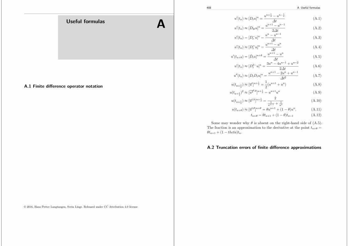
Useful formulas A
A.1 Finite difference operator notation
© 2016, Hans Petter Langtangen, Svein Linge. Released under CC Attribution 4.0 license
488 A Useful formulas
u′(tn) ≈ [Dtu]n = un+ 12 − un− 1
2
∆t(A.1)
u′(tn) ≈ [D2tu]n = un+1 − un−1
2∆t (A.2)
u′(tn) = [D−t u]n = un − un−1
∆t(A.3)
u′(tn) ≈ [D+t u]n = un+1 − un
∆t(A.4)
u′(tn+θ) = [Dtu]n+θ = un+1 − un∆t
(A.5)
u′(tn) ≈ [D2−t u]n = 3un − 4un−1 + un−2
2∆t (A.6)
u′′(tn) ≈ [DtDtu]n = un+1 − 2un + un−1
∆t2(A.7)
u(tn+ 12) ≈ [ut]n+ 1
2 = 12(un+1 + un) (A.8)
u(tn+ 12)2 ≈ [u2t,g]n+ 1
2 = un+1un (A.9)
u(tn+ 12) ≈ [ut,h]n+ 1
2 = 21
un+1 + 1un
(A.10)
u(tn+θ) ≈ [ut,θ]n+θ = θun+1 + (1− θ)un, (A.11)tn+θ = θtn+1 + (1− θ)tn−1 (A.12)
Some may wonder why θ is absent on the right-hand side of (A.5).The fraction is an approximation to the derivative at the point tn+θ =θtn+1 + (1− theta)tn.
A.2 Truncation errors of finite difference approximations
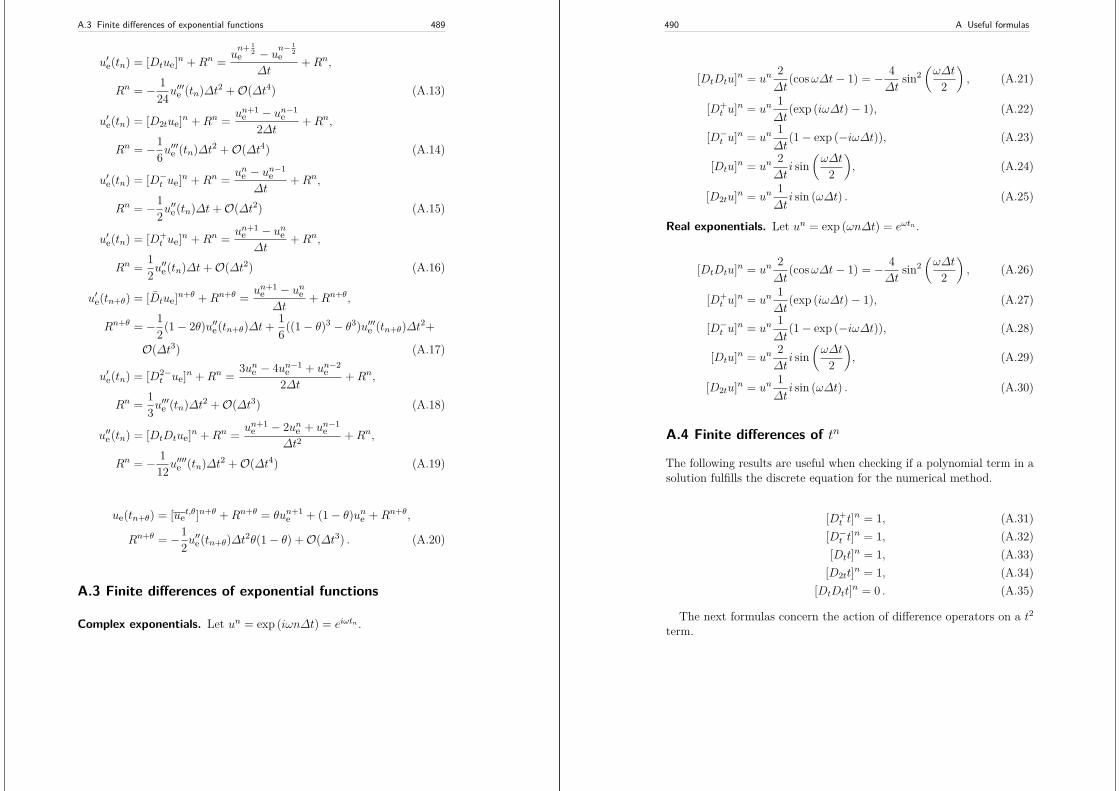
A.3 Finite differences of exponential functions 489
u′e(tn) = [Dtue]n +Rn = un+ 1
2e − un−12e
∆t+Rn,
Rn = − 124u
′′′e (tn)∆t2 +O(∆t4) (A.13)
u′e(tn) = [D2tue]n +Rn = un+1e − un−1
e2∆t +Rn,
Rn = −16u′′′e (tn)∆t2 +O(∆t4) (A.14)
u′e(tn) = [D−t ue]n +Rn = une − un−1e
∆t+Rn,
Rn = −12u′′e(tn)∆t+O(∆t2) (A.15)
u′e(tn) = [D+t ue]n +Rn = un+1
e − une∆t
+Rn,
Rn = 12u′′e(tn)∆t+O(∆t2) (A.16)
u′e(tn+θ) = [Dtue]n+θ +Rn+θ = un+1e − une∆t
+Rn+θ,
Rn+θ = −12(1− 2θ)u′′e(tn+θ)∆t+ 1
6((1− θ)3 − θ3)u′′′e (tn+θ)∆t2+
O(∆t3) (A.17)
u′e(tn) = [D2−t ue]n +Rn = 3une − 4un−1
e + un−2e
2∆t +Rn,
Rn = 13u′′′e (tn)∆t2 +O(∆t3) (A.18)
u′′e(tn) = [DtDtue]n +Rn = un+1e − 2une + un−1
e∆t2
+Rn,
Rn = − 112u
′′′′e (tn)∆t2 +O(∆t4) (A.19)
ue(tn+θ) = [uet,θ]n+θ +Rn+θ = θun+1e + (1− θ)une +Rn+θ,
Rn+θ = −12u′′e(tn+θ)∆t2θ(1− θ) +O(∆t3) . (A.20)
A.3 Finite differences of exponential functions
Complex exponentials. Let un = exp (iωn∆t) = eiωtn .
490 A Useful formulas
[DtDtu]n = un2∆t
(cosω∆t− 1) = − 4∆t
sin2(ω∆t
2
), (A.21)
[D+t u]n = un
1∆t
(exp (iω∆t)− 1), (A.22)
[D−t u]n = un1∆t
(1− exp (−iω∆t)), (A.23)
[Dtu]n = un2∆t
i sin(ω∆t
2
), (A.24)
[D2tu]n = un1∆t
i sin (ω∆t) . (A.25)
Real exponentials. Let un = exp (ωn∆t) = eωtn .
[DtDtu]n = un2∆t
(cosω∆t− 1) = − 4∆t
sin2(ω∆t
2
), (A.26)
[D+t u]n = un
1∆t
(exp (iω∆t)− 1), (A.27)
[D−t u]n = un1∆t
(1− exp (−iω∆t)), (A.28)
[Dtu]n = un2∆t
i sin(ω∆t
2
), (A.29)
[D2tu]n = un1∆t
i sin (ω∆t) . (A.30)
A.4 Finite differences of tn
The following results are useful when checking if a polynomial term in asolution fulfills the discrete equation for the numerical method.
[D+t t]n = 1, (A.31)
[D−t t]n = 1, (A.32)[Dtt]n = 1, (A.33)
[D2tt]n = 1, (A.34)[DtDtt]n = 0 . (A.35)
The next formulas concern the action of difference operators on a t2term.
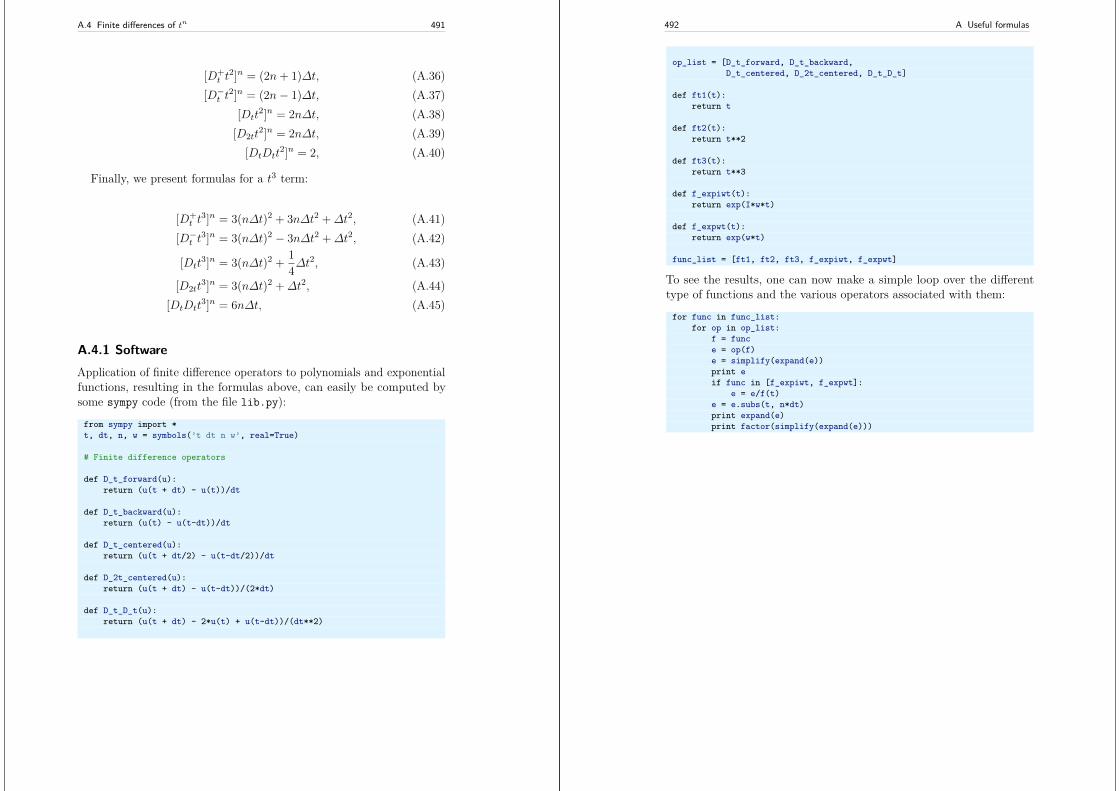
A.4 Finite differences of tn 491
[D+t t
2]n = (2n+ 1)∆t, (A.36)[D−t t2]n = (2n− 1)∆t, (A.37)
[Dtt2]n = 2n∆t, (A.38)
[D2tt2]n = 2n∆t, (A.39)
[DtDtt2]n = 2, (A.40)
Finally, we present formulas for a t3 term:
[D+t t
3]n = 3(n∆t)2 + 3n∆t2 +∆t2, (A.41)[D−t t3]n = 3(n∆t)2 − 3n∆t2 +∆t2, (A.42)
[Dtt3]n = 3(n∆t)2 + 1
4∆t2, (A.43)
[D2tt3]n = 3(n∆t)2 +∆t2, (A.44)
[DtDtt3]n = 6n∆t, (A.45)
A.4.1 SoftwareApplication of finite difference operators to polynomials and exponentialfunctions, resulting in the formulas above, can easily be computed bysome sympy code (from the file lib.py):
from sympy import *t, dt, n, w = symbols(’t dt n w’, real=True)
# Finite difference operators
def D_t_forward(u):return (u(t + dt) - u(t))/dt
def D_t_backward(u):return (u(t) - u(t-dt))/dt
def D_t_centered(u):return (u(t + dt/2) - u(t-dt/2))/dt
def D_2t_centered(u):return (u(t + dt) - u(t-dt))/(2*dt)
def D_t_D_t(u):return (u(t + dt) - 2*u(t) + u(t-dt))/(dt**2)
492 A Useful formulas
op_list = [D_t_forward, D_t_backward,D_t_centered, D_2t_centered, D_t_D_t]
def ft1(t):return t
def ft2(t):return t**2
def ft3(t):return t**3
def f_expiwt(t):return exp(I*w*t)
def f_expwt(t):return exp(w*t)
func_list = [ft1, ft2, ft3, f_expiwt, f_expwt]
To see the results, one can now make a simple loop over the differenttype of functions and the various operators associated with them:
for func in func_list:for op in op_list:
f = funce = op(f)e = simplify(expand(e))print eif func in [f_expiwt, f_expwt]:
e = e/f(t)e = e.subs(t, n*dt)print expand(e)print factor(simplify(expand(e)))
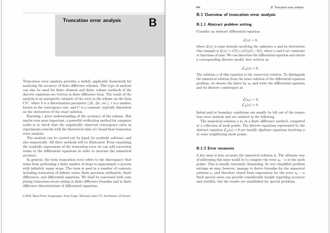
Truncation error analysis B
Truncation error analysis provides a widely applicable framework foranalyzing the accuracy of finite difference schemes. This type of analysiscan also be used for finite element and finite volume methods if thediscrete equations are written in finite difference form. The result of theanalysis is an asymptotic estimate of the error in the scheme on the formChr, where h is a discretization parameter (∆t, ∆x, etc.), r is a number,known as the convergence rate, and C is a constant, typically dependenton the derivatives of the exact solution.
Knowing r gives understanding of the accuracy of the scheme. Butmaybe even more important, a powerful verification method for computercodes is to check that the empirically observed convergence rates inexperiments coincide with the theoretical value of r found from truncationerror analysis.
The analysis can be carried out by hand, by symbolic software, andalso numerically. All three methods will be illustrated. From examiningthe symbolic expressions of the truncation error we can add correctionterms to the differential equations in order to increase the numericalaccuracy.
In general, the term truncation error refers to the discrepancy thatarises from performing a finite number of steps to approximate a processwith infinitely many steps. The term is used in a number of contexts,including truncation of infinite series, finite precision arithmetic, finitedifferences, and differential equations. We shall be concerned with com-puting truncation errors arising in finite difference formulas and in finitedifference discretizations of differential equations.
© 2016, Hans Petter Langtangen, Svein Linge. Released under CC Attribution 4.0 license
494 B Truncation error analysis
B.1 Overview of truncation error analysis
B.1.1 Abstract problem setting
Consider an abstract differential equation
L(u) = 0,
where L(u) is some formula involving the unknown u and its derivatives.One example is L(u) = u′(t)+a(t)u(t)−b(t), where a and b are constantsor functions of time. We can discretize the differential equation and obtaina corresponding discrete model, here written as
L∆(u) = 0 .
The solution u of this equation is the numerical solution. To distinguishthe numerical solution from the exact solution of the differential equationproblem, we denote the latter by ue and write the differential equationand its discrete counterpart as
L(ue) = 0,L∆(u) = 0 .
Initial and/or boundary conditions can usually be left out of the trunca-tion error analysis and are omitted in the following.
The numerical solution u is, in a finite difference method, computedat a collection of mesh points. The discrete equations represented by theabstract equation L∆(u) = 0 are usually algebraic equations involving uat some neighboring mesh points.
B.1.2 Error measures
A key issue is how accurate the numerical solution is. The ultimate wayof addressing this issue would be to compute the error ue−u at the meshpoints. This is usually extremely demanding. In very simplified problemsettings we may, however, manage to derive formulas for the numericalsolution u, and therefore closed form expressions for the error ue − u.Such special cases can provide considerable insight regarding accuracyand stability, but the results are established for special problems.
B.1 Overview of truncation error analysis 495
The error ue−u can be computed empirically in special cases where weknow ue. Such cases can be constructed by the method of manufacturedsolutions, where we choose some exact solution ue = v and fit a sourceterm f in the governing differential equation L(ue) = f such that ue = vis a solution (i.e., f = L(v)). Assuming an error model of the formChr, where h is the discretization parameter, such as ∆t or ∆x, one canestimate the convergence rate r. This is a widely applicable procedure,but the validity of the results is, strictly speaking, tied to the chosen testproblems.
Another error measure arises by asking to what extent the exactsolution ue fits the discrete equations. Clearly, ue is in general not asolution of L∆(u) = 0, but we can define the residual
R = L∆(ue),
and investigate how close R is to zero. A small R means intuitively thatthe discrete equations are close to the differential equation, and then weare tempted to think that un must also be close to ue(tn).
The residual R is known as the truncation error of the finite differencescheme L∆(u) = 0. It appears that the truncation error is relativelystraightforward to compute by hand or symbolic software without special-izing the differential equation and the discrete model to a special case. Theresulting R is found as a power series in the discretization parameters.The leading-order terms in the series provide an asymptotic measureof the accuracy of the numerical solution method (as the discretizationparameters tend to zero). An advantage of truncation error analysis, com-pared to empirical estimation of convergence rates, or detailed analysisof a special problem with a mathematical expression for the numericalsolution, is that the truncation error analysis reveals the accuracy of thevarious building blocks in the numerical method and how each buildingblock impacts the overall accuracy. The analysis can therefore be usedto detect building blocks with lower accuracy than the others.
Knowing the truncation error or other error measures is important forverification of programs by empirically establishing convergence rates.The forthcoming text will provide many examples on how to computetruncation errors for finite difference discretizations of ODEs and PDEs.
496 B Truncation error analysis
B.2 Truncation errors in finite difference formulas
The accuracy of a finite difference formula is a fundamental issue whendiscretizing differential equations. We shall first go through a particularexample in detail and thereafter list the truncation error in the mostcommon finite difference approximation formulas.
B.2.1 Example: The backward difference for u′(t)
Consider a backward finite difference approximation of the first-orderderivative u′:
[D−t u]n = un − un−1
∆t≈ u′(tn) . (B.1)
Here, un means the value of some function u(t) at a point tn, and[D−t u]n is the discrete derivative of u(t) at t = tn. The discrete derivativecomputed by a finite difference is, in general, not exactly equal to thederivative u′(tn). The error in the approximation is
Rn = [D−t u]n − u′(tn) . (B.2)
The common way of calculating Rn is to
1. expand u(t) in a Taylor series around the point where the derivativeis evaluated, here tn,
2. insert this Taylor series in (B.2), and3. collect terms that cancel and simplify the expression.
The result is an expression for Rn in terms of a power series in ∆t. Theerror Rn is commonly referred to as the truncation error of the finitedifference formula.
The Taylor series formula often found in calculus books takes the form
f(x+ h) =∞∑
i=0
1i!dif
dxi(x)hi .
In our application, we expand the Taylor series around the point wherethe finite difference formula approximates the derivative. The Taylorseries of un at tn is simply u(tn), while the Taylor series of un−1 at tnmust employ the general formula,
B.2 Truncation errors in finite difference formulas 497
u(tn−1) = u(t−∆t) =∞∑
i=0
1i!diu
dti(tn)(−∆t)i
= u(tn)− u′(tn)∆t+ 12u′′(tn)∆t2 +O(∆t3),
where O(∆t3) means a power-series in ∆t where the lowest power is ∆t3.We assume that ∆t is small such that ∆tp ∆tq if p is smaller than q.The details of higher-order terms in ∆t are therefore not of much interest.Inserting the Taylor series above in the right-hand side of1 (B.2) givesrise to some algebra:
[D−t u]n − u′(tn) = u(tn)− u(tn−1)∆t
− u′(tn)
=u(tn)− (u(tn)− u′(tn)∆t+ 1
2u′′(tn)∆t2 +O(∆t3))
∆t− u′(tn)
= −12u′′(tn)∆t+O(∆t2)),
which is, according to (B.2), the truncation error:
Rn = −12u′′(tn)∆t+O(∆t2)) . (B.3)
The dominating term for small ∆t is −12u′′(tn)∆t, which is proportional
to ∆t, and we say that the truncation error is of first order in ∆t.
B.2.2 Example: The forward difference for u′(t)
We can analyze the approximation error in the forward difference
u′(tn) ≈ [D+t u]n = un+1 − un
∆t,
by writingRn = [D+
t u]n − u′(tn),
and expanding un+1 in a Taylor series around tn,
u(tn+1) = u(tn) + u′(tn)∆t+ 12u′′(tn)∆t2 +O(∆t3) .
The result becomes
498 B Truncation error analysis
R = 12u′′(tn)∆t+O(∆t2),
showing that also the forward difference is of first order.
B.2.3 Example: The central difference for u′(t)
For the central difference approximation,
u′(tn) ≈ [Dtu]n, [Dtu]n = un+ 12 − un− 1
2
∆t,
we write
Rn = [Dtu]n − u′(tn),
and expand u(tn+ 12) and u(tn− 1
2in Taylor series around the point tn
where the derivative is evaluated. We have
u(tn+ 12) =u(tn) + u′(tn)1
2∆t+ 12u′′(tn)(1
2∆t)2+
16u′′′(tn)(1
2∆t)3 + 1
24u′′′′(tn)(1
2∆t)4+
1120u
′′′′(tn)(12∆t)
5 +O(∆t6),
u(tn− 12) =u(tn)− u′(tn)1
2∆t+ 12u′′(tn)(1
2∆t)2−
16u′′′(tn)(1
2∆t)3 + 1
24u′′′′(tn)(1
2∆t)4−
1120u
′′′′′(tn)(12∆t)
5 +O(∆t6) .
Now,
u(tn+ 12)−u(tn− 1
2) = u′(tn)∆t+ 1
24u′′′(tn)∆t3+ 1
960u′′′′′(tn)∆t5+O(∆t7) .
By collecting terms in [Dtu]n − u′(tn) we find the truncation error to be
Rn = 124u
′′′(tn)∆t2 +O(∆t4), (B.4)
with only even powers of∆t. Since R ∼ ∆t2 we say the centered differenceis of second order in ∆t.
B.2 Truncation errors in finite difference formulas 499
B.2.4 Overview of leading-order error terms in finitedifference formulas
Here we list the leading-order terms of the truncation errors associatedwith several common finite difference formulas for the first and secondderivatives.
[Dtu]n = un+ 12 − un− 1
2
∆t= u′(tn) +Rn, (B.5)
Rn = 124u
′′′(tn)∆t2 +O(∆t4) (B.6)
[D2tu]n = un+1 − un−1
2∆t = u′(tn) +Rn, (B.7)
Rn = 16u′′′(tn)∆t2 +O(∆t4) (B.8)
[D−t u]n = un − un−1
∆t= u′(tn) +Rn, (B.9)
Rn = −12u′′(tn)∆t+O(∆t2) (B.10)
[D+t u]n = un+1 − un
∆t= u′(tn) +Rn, (B.11)
Rn = 12u′′(tn)∆t+O(∆t2) (B.12)
[Dtu]n+θ = un+1 − un∆t
= u′(tn+θ) +Rn+θ, (B.13)
Rn+θ = 12(1− 2θ)u′′(tn+θ)∆t−
16((1− θ)3 − θ3)u′′′(tn+θ)∆t2 +O(∆t3)
(B.14)
[D2−t u]n = 3un − 4un−1 + un−2
2∆t = u′(tn) +Rn, (B.15)
Rn = −13u′′′(tn)∆t2 +O(∆t3) (B.16)
[DtDtu]n = un+1 − 2un + un−1
∆t2= u′′(tn) +Rn, (B.17)
Rn = 112u
′′′′(tn)∆t2 +O(∆t4) (B.18)
It will also be convenient to have the truncation errors for variousmeans or averages. The weighted arithmetic mean leads to
500 B Truncation error analysis
[ut,θ]n+θ = θun+1 + (1− θ)un = u(tn+θ) +Rn+θ, (B.19)
Rn+θ = 12u′′(tn+θ)∆t2θ(1− θ) +O(∆t3) . (B.20)
The standard arithmetic mean follows from this formula when θ = 12 .
Expressed at point tn we get
[ut]n = 12(un− 1
2 + un+ 12 ) = u(tn) +Rn, (B.21)
Rn = 18u′′(tn)∆t2 + 1
384u′′′′(tn)∆t4 +O(∆t6) . (B.22)
The geometric mean also has an error O(∆t2):
[u2t,g]n = un−12un+ 1
2 = (un)2 +Rn, (B.23)
Rn = −14u′(tn)2∆t2 + 1
4u(tn)u′′(tn)∆t2 +O(∆t4) . (B.24)
The harmonic mean is also second-order accurate:
[ut,h]n = un = 21
un−12
+ 1un+ 1
2
+Rn+ 12 , (B.25)
Rn = −u′(tn)2
4u(tn)∆t2 + 1
8u′′(tn)∆t2 . (B.26)
B.2.5 Software for computing truncation errors
We can use sympy to aid calculations with Taylor series. The derivativescan be defined as symbols, say D3f for the 3rd derivative of some func-tion f . A truncated Taylor series can then be written as f + D1f*h +D2f*h**2/2. The following class takes some symbol f for the function inquestion and makes a list of symbols for the derivatives. The __call__method computes the symbolic form of the series truncated at num_termsterms.
import sympy as sym
class TaylorSeries:"""Class for symbolic Taylor series."""def __init__(self, f, num_terms=4):
B.2 Truncation errors in finite difference formulas 501
self.f = fself.N = num_terms# Introduce symbols for the derivativesself.df = [f]for i in range(1, self.N+1):
self.df.append(sym.Symbol(’D%d%s’ % (i, f.name)))
def __call__(self, h):"""Return the truncated Taylor series at x+h."""terms = self.ffor i in range(1, self.N+1):
terms += sym.Rational(1, sym.factorial(i))*self.df[i]*h**ireturn terms
We may, for example, use this class to compute the truncation errorof the Forward Euler finite difference formula:
>>> from truncation_errors import TaylorSeries>>> from sympy import *>>> u, dt = symbols(’u dt’)>>> u_Taylor = TaylorSeries(u, 4)>>> u_Taylor(dt)D1u*dt + D2u*dt**2/2 + D3u*dt**3/6 + D4u*dt**4/24 + u>>> FE = (u_Taylor(dt) - u)/dt>>> FE(D1u*dt + D2u*dt**2/2 + D3u*dt**3/6 + D4u*dt**4/24)/dt>>> simplify(FE)D1u + D2u*dt/2 + D3u*dt**2/6 + D4u*dt**3/24
The truncation error consists of the terms after the first one (u′).The module file trunc/truncation_errors.py contains another class
DiffOp with symbolic expressions for most of the truncation errors listedin the previous section. For example:
>>> from truncation_errors import DiffOp>>> from sympy import *>>> u = Symbol(’u’)>>> diffop = DiffOp(u, independent_variable=’t’)>>> diffop[’geometric_mean’]-D1u**2*dt**2/4 - D1u*D3u*dt**4/48 + D2u**2*dt**4/64 + ...>>> diffop[’Dtm’]D1u + D2u*dt/2 + D3u*dt**2/6 + D4u*dt**3/24>>> >>> diffop.operator_names()[’geometric_mean’, ’harmonic_mean’, ’Dtm’, ’D2t’, ’DtDt’,’weighted_arithmetic_mean’, ’Dtp’, ’Dt’]
The indexing of diffop applies names that correspond to the operators:Dtp for D+
t , Dtm for D−t , Dt for Dt, D2t for D2t, DtDt for DtDt.
502 B Truncation error analysis
B.3 Exponential decay ODEs
We shall now compute the truncation error of a finite difference schemefor a differential equation. Our first problem involves the following thelinear ODE modeling exponential decay,
u′(t) = −au(t) . (B.27)
B.3.1 Forward Euler scheme
We begin with the Forward Euler scheme for discretizing (B.27):
[D+t u = −au]n . (B.28)
The idea behind the truncation error computation is to insert the exactsolution ue of the differential equation problem (B.27) in the discreteequations (B.28) and find the residual that arises because ue does notsolve the discrete equations. Instead, ue solves the discrete equationswith a residual Rn:
[D+t ue + aue = R]n . (B.29)
From (B.11)-(B.12) it follows that
[D+t ue]n = u′e(tn) + 1
2u′′e(tn)∆t+O(∆t2),
which inserted in (B.29) results in
u′e(tn) + 12u′′e(tn)∆t+O(∆t2) + aue(tn) = Rn .
Now, u′e(tn) + aune = 0 since ue solves the differential equation. Theremaining terms constitute the residual:
Rn = 12u′′e(tn)∆t+O(∆t2) . (B.30)
This is the truncation error Rn of the Forward Euler scheme.Because Rn is proportional to ∆t, we say that the Forward Euler
scheme is of first order in ∆t. However, the truncation error is just oneerror measure, and it is not equal to the true error une − un. For thissimple model problem we can compute a range of different error measures
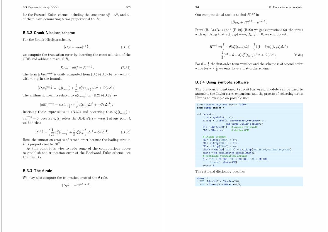
B.3 Exponential decay ODEs 503
for the Forward Euler scheme, including the true error une − un, and allof them have dominating terms proportional to ∆t.
B.3.2 Crank-Nicolson schemeFor the Crank-Nicolson scheme,
[Dtu = −au]n+ 12 , (B.31)
we compute the truncation error by inserting the exact solution of theODE and adding a residual R,
[Dtue + auet = R]n+ 1
2 . (B.32)
The term [Dtue]n+ 12 is easily computed from (B.5)-(B.6) by replacing n
with n+ 12 in the formula,
[Dtue]n+ 12 = u′e(tn+ 1
2) + 1
24u′′′e (tn+ 1
2)∆t2 +O(∆t4) .
The arithmetic mean is related to u(tn+ 12) by (B.21)-(B.22) so
[auet]n+ 12 = ue(tn+ 1
2) + 1
8u′′e(tn)∆t2 + +O(∆t4) .
Inserting these expressions in (B.32) and observing that u′e(tn+ 12) +
aun+ 1
2e = 0, because ue(t) solves the ODE u′(t) = −au(t) at any point t,we find that
Rn+ 12 =
( 124u
′′′e (tn+ 1
2) + 1
8u′′e(tn)
)∆t2 +O(∆t4) (B.33)
Here, the truncation error is of second order because the leading term inR is proportional to ∆t2.
At this point it is wise to redo some of the computations aboveto establish the truncation error of the Backward Euler scheme, seeExercise B.7.
B.3.3 The θ-ruleWe may also compute the truncation error of the θ-rule,
[Dtu = −aut,θ]n+θ .
504 B Truncation error analysis
Our computational task is to find Rn+θ in
[Dtue + auet,θ = R]n+θ .
From (B.13)-(B.14) and (B.19)-(B.20) we get expressions for the termswith ue. Using that u′e(tn+θ) + aue(tn+θ) = 0, we end up with
Rn+θ =(12 − θ)u
′′e(tn+θ)∆t+ 1
2θ(1− θ)u′′e(tn+θ)∆t2+
12(θ2 − θ + 3)u′′′e (tn+θ)∆t2 +O(∆t3) (B.34)
For θ = 12 the first-order term vanishes and the scheme is of second order,
while for θ 6= 12 we only have a first-order scheme.
B.3.4 Using symbolic software
The previously mentioned truncation_error module can be used toautomate the Taylor series expansions and the process of collecting terms.Here is an example on possible use:
from truncation_error import DiffOpfrom sympy import *
def decay():u, a = symbols(’u a’)diffop = DiffOp(u, independent_variable=’t’,
num_terms_Taylor_series=3)D1u = diffop.D(1) # symbol for du/dtODE = D1u + a*u # define ODE
# Define schemesFE = diffop[’Dtp’] + a*uCN = diffop[’Dt’ ] + a*uBE = diffop[’Dtm’] + a*utheta = diffop[’barDt’] + a*diffop[’weighted_arithmetic_mean’]theta = sm.simplify(sm.expand(theta))# Residuals (truncation errors)R = ’FE’: FE-ODE, ’BE’: BE-ODE, ’CN’: CN-ODE,
’theta’: theta-ODEreturn R
The returned dictionary becomes
decay: ’BE’: D2u*dt/2 + D3u*dt**2/6,’FE’: -D2u*dt/2 + D3u*dt**2/6,
B.3 Exponential decay ODEs 505
’CN’: D3u*dt**2/24,’theta’: -D2u*a*dt**2*theta**2/2 + D2u*a*dt**2*theta/2 -
D2u*dt*theta + D2u*dt/2 + D3u*a*dt**3*theta**3/3 -D3u*a*dt**3*theta**2/2 + D3u*a*dt**3*theta/6 +D3u*dt**2*theta**2/2 - D3u*dt**2*theta/2 + D3u*dt**2/6,
The results are in correspondence with our hand-derived expressions.
B.3.5 Empirical verification of the truncation error
The task of this section is to demonstrate how we can compute thetruncation error R numerically. For example, the truncation error of theForward Euler scheme applied to the decay ODE u′ = −ua is
Rn = [D+t ue + aue]n . (B.35)
If we happen to know the exact solution ue(t), we can easily evaluateRn from the above formula.
To estimate how R varies with the discretization parameter ∆t, whichhas been our focus in the previous mathematical derivations, we firstmake the assumption that R = C∆tr for appropriate constants C andr and small enough ∆t. The rate r can be estimated from a seriesof experiments where ∆t is varied. Suppose we have m experiments(∆ti, Ri), i = 0, . . . ,m−1. For two consecutive experiments (∆ti−1, Ri−1)and (∆ti, Ri), a corresponding ri−1 can be estimated by
ri−1 = ln(Ri−1/Ri)ln(∆ti−1/∆ti)
, (B.36)
for i = 1, . . . ,m − 1. Note that the truncation error Ri varies throughthe mesh, so (B.36) is to be applied pointwise. A complicating issue isthat Ri and Ri−1 refer to different meshes. Pointwise comparisons ofthe truncation error at a certain point in all meshes therefore requiresany computed R to be restricted to the coarsest mesh and that all finermeshes contain all the points in the coarsest mesh. Suppose we have N0intervals in the coarsest mesh. Inserting a superscript n in (B.36), wheren counts mesh points in the coarsest mesh, n = 0, . . . , N0, leads to theformula
rni−1 = ln(Rni−1/Rni )
ln(∆ti−1/∆ti). (B.37)
506 B Truncation error analysis
Experiments are most conveniently defined by N0 and a number ofrefinements m. Suppose each mesh has twice as many cells Ni as theprevious one:
Ni = 2iN0, ∆ti = TN−1i ,
where [0, T ] is the total time interval for the computations. Suppose thecomputed Ri values on the mesh with Ni intervals are stored in an arrayR[i] (R being a list of arrays, one for each mesh). Restricting this Rifunction to the coarsest mesh means extracting every Ni/N0 point andis done as follows:
stride = N[i]/N_0R[i] = R[i][::stride]
The quantity R[i][n] now corresponds to Rni .In addition to estimating r for the pointwise values of R = C∆tr, we
may also consider an integrated quantity on mesh i,
RI,i =(∆ti
Ni∑
n=0(Rni )2
) 12
≈∫ T
0Ri(t)dt . (B.38)
The sequence RI,i, i = 0, . . . ,m− 1, is also expected to behave as C∆tr,with the same r as for the pointwise quantity R, as ∆t→ 0.
The function below computes the Ri and RI,i quantities, plots themand compares with the theoretically derived truncation error (R_a) ifavailable.
import numpy as npimport scitools.std as plt
def estimate(truncation_error, T, N_0, m, makeplot=True):"""Compute the truncation error in a problem with one independentvariable, using m meshes, and estimate the convergencerate of the truncation error.
The user-supplied function truncation_error(dt, N) computesthe truncation error on a uniform mesh with N intervals oflength dt::
R, t, R_a = truncation_error(dt, N)
where R holds the truncation error at points in the array t,and R_a are the corresponding theoretical truncation errorvalues (None if not available).
The truncation_error function is run on a series of mesheswith 2**i*N_0 intervals, i=0,1,...,m-1.
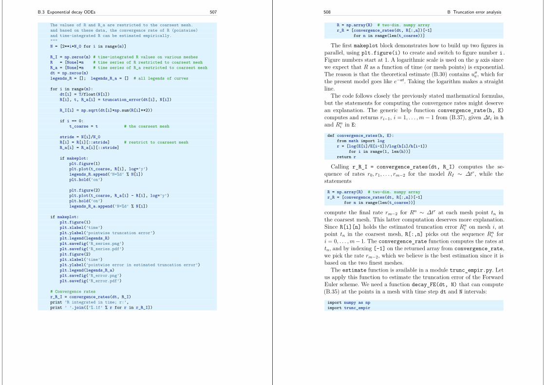
B.3 Exponential decay ODEs 507
The values of R and R_a are restricted to the coarsest mesh.and based on these data, the convergence rate of R (pointwise)and time-integrated R can be estimated empirically."""N = [2**i*N_0 for i in range(m)]
R_I = np.zeros(m) # time-integrated R values on various meshesR = [None]*m # time series of R restricted to coarsest meshR_a = [None]*m # time series of R_a restricted to coarsest meshdt = np.zeros(m)legends_R = []; legends_R_a = [] # all legends of curves
for i in range(m):dt[i] = T/float(N[i])R[i], t, R_a[i] = truncation_error(dt[i], N[i])
R_I[i] = np.sqrt(dt[i]*np.sum(R[i]**2))
if i == 0:t_coarse = t # the coarsest mesh
stride = N[i]/N_0R[i] = R[i][::stride] # restrict to coarsest meshR_a[i] = R_a[i][::stride]
if makeplot:plt.figure(1)plt.plot(t_coarse, R[i], log=’y’)legends_R.append(’N=%d’ % N[i])plt.hold(’on’)
plt.figure(2)plt.plot(t_coarse, R_a[i] - R[i], log=’y’)plt.hold(’on’)legends_R_a.append(’N=%d’ % N[i])
if makeplot:plt.figure(1)plt.xlabel(’time’)plt.ylabel(’pointwise truncation error’)plt.legend(legends_R)plt.savefig(’R_series.png’)plt.savefig(’R_series.pdf’)plt.figure(2)plt.xlabel(’time’)plt.ylabel(’pointwise error in estimated truncation error’)plt.legend(legends_R_a)plt.savefig(’R_error.png’)plt.savefig(’R_error.pdf’)
# Convergence ratesr_R_I = convergence_rates(dt, R_I)print ’R integrated in time; r:’,print ’ ’.join([’%.1f’ % r for r in r_R_I])
508 B Truncation error analysis
R = np.array(R) # two-dim. numpy arrayr_R = [convergence_rates(dt, R[:,n])[-1]
for n in range(len(t_coarse))]
The first makeplot block demonstrates how to build up two figures inparallel, using plt.figure(i) to create and switch to figure number i.Figure numbers start at 1. A logarithmic scale is used on the y axis sincewe expect that R as a function of time (or mesh points) is exponential.The reason is that the theoretical estimate (B.30) contains u′′e , which forthe present model goes like e−at. Taking the logarithm makes a straightline.
The code follows closely the previously stated mathematical formulas,but the statements for computing the convergence rates might deservean explanation. The generic help function convergence_rate(h, E)computes and returns ri−1, i = 1, . . . ,m− 1 from (B.37), given ∆ti in hand Rni in E:
def convergence_rates(h, E):from math import logr = [log(E[i]/E[i-1])/log(h[i]/h[i-1])
for i in range(1, len(h))]return r
Calling r_R_I = convergence_rates(dt, R_I) computes the se-quence of rates r0, r1, . . . , rm−2 for the model RI ∼ ∆tr, while thestatements
R = np.array(R) # two-dim. numpy arrayr_R = [convergence_rates(dt, R[:,n])[-1]
for n in range(len(t_coarse))]
compute the final rate rm−2 for Rn ∼ ∆tr at each mesh point tn inthe coarsest mesh. This latter computation deserves more explanation.Since R[i][n] holds the estimated truncation error Rni on mesh i, atpoint tn in the coarsest mesh, R[:,n] picks out the sequence Rni fori = 0, . . . ,m− 1. The convergence_rate function computes the rates attn, and by indexing [-1] on the returned array from convergence_rate,we pick the rate rm−2, which we believe is the best estimation since it isbased on the two finest meshes.
The estimate function is available in a module trunc_empir.py. Letus apply this function to estimate the truncation error of the ForwardEuler scheme. We need a function decay_FE(dt, N) that can compute(B.35) at the points in a mesh with time step dt and N intervals:
import numpy as npimport trunc_empir
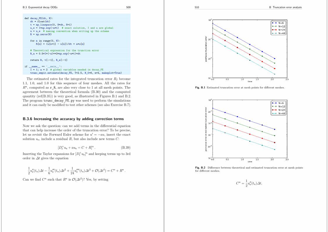
B.3 Exponential decay ODEs 509
def decay_FE(dt, N):dt = float(dt)t = np.linspace(0, N*dt, N+1)u_e = I*np.exp(-a*t) # exact solution, I and a are globalu = u_e # naming convention when writing up the schemeR = np.zeros(N)
for n in range(0, N):R[n] = (u[n+1] - u[n])/dt + a*u[n]
# Theoretical expression for the trunction errorR_a = 0.5*I*(-a)**2*np.exp(-a*t)*dt
return R, t[:-1], R_a[:-1]
if __name__ == ’__main__’:I = 1; a = 2 # global variables needed in decay_FEtrunc_empir.estimate(decay_FE, T=2.5, N_0=6, m=4, makeplot=True)
The estimated rates for the integrated truncation error RI become1.1, 1.0, and 1.0 for this sequence of four meshes. All the rates forRn, computed as r_R, are also very close to 1 at all mesh points. Theagreement between the theoretical formula (B.30) and the computedquantity (ref(B.35)) is very good, as illustrated in Figures B.1 and B.2.The program trunc_decay_FE.py was used to perform the simulationsand it can easily be modified to test other schemes (see also Exercise B.7).
B.3.6 Increasing the accuracy by adding correction terms
Now we ask the question: can we add terms in the differential equationthat can help increase the order of the truncation error? To be precise,let us revisit the Forward Euler scheme for u′ = −au, insert the exactsolution ue, include a residual R, but also include new terms C:
[D+t ue + aue = C +R]n . (B.39)
Inserting the Taylor expansions for [D+t ue]n and keeping terms up to 3rd
order in ∆t gives the equation
12u′′e(tn)∆t− 1
6u′′′e (tn)∆t2 + 1
24u′′′′e (tn)∆t3 +O(∆t4) = Cn +Rn .
Can we find Cn such that Rn is O(∆t2)? Yes, by setting
510 B Truncation error analysis
Fig. B.1 Estimated truncation error at mesh points for different meshes.
Fig. B.2 Difference between theoretical and estimated truncation error at mesh pointsfor different meshes.
Cn = 12u′′e(tn)∆t,
B.3 Exponential decay ODEs 511
we manage to cancel the first-order term and
Rn = 16u′′′e (tn)∆t2 +O(∆t3) .
The correction term Cn introduces 12∆tu
′′ in the discrete equation,and we have to get rid of the derivative u′′. One idea is to approximateu′′ by a second-order accurate finite difference formula, u′′ ≈ (un+1 −2un + un−1)/∆t2, but this introduces an additional time level with un−1.Another approach is to rewrite u′′ in terms of u′ or u using the ODE:
u′ = −au ⇒ u′′ = −au′ = −a(−au) = a2u .
This means that we can simply set Cn = 12a
2∆tun. We can then eithersolve the discrete equation
[D+t u = −au+ 1
2a2∆tu]n, (B.40)
or we can equivalently discretize the perturbed ODE
u′ = −au, a = a(1− 12a∆t), (B.41)
by a Forward Euler method. That is, we replace the original coefficient aby the perturbed coefficient a. Observe that a→ a as ∆t→ 0.
The Forward Euler method applied to (B.41) results in
[D+t u = −a(1− 1
2a∆t)u]n .
We can control our computations and verify that the truncation error ofthe scheme above is indeed O(∆t2).
Another way of revealing the fact that the perturbed ODE leads to amore accurate solution is to look at the amplification factor. Our schemecan be written as
un+1 = Aun, A = 1− a∆t = 1− p+ 12p
2, p = a∆t,
The amplification factor A as a function of p = a∆t is seen to be the firstthree terms of the Taylor series for the exact amplification factor e−p.The Forward Euler scheme for u = −au gives only the first two terms1− p of the Taylor series for e−p. That is, using a increases the order ofthe accuracy in the amplification factor.
512 B Truncation error analysis
Instead of replacing u′′ by a2u, we use the relation u′′ = −au′ and adda term −1
2a∆tu′ in the ODE:
u′ = −au− 12a∆tu
′ ⇒(
1 + 12a∆t
)u′ = −au .
Using a Forward Euler method results in(
1 + 12a∆t
)un+1 − un
∆t= −aun,
which after some algebra can be written as
un+1 =1− 1
2a∆t
1 + 12a∆t
un .
This is the same formula as the one arising from a Crank-Nicolson schemeapplied to u′ = −au! It now recommended to do Exercise B.7 and repeatthe above steps to see what kind of correction term is needed in theBackward Euler scheme to make it second order.
The Crank-Nicolson scheme is a bit more challenging to analyze, butthe ideas and techniques are the same. The discrete equation reads
[Dtu = −au]n+ 12 ,
and the truncation error is defined through
[Dtue + auet = C +R]n+ 1
2 ,
where we have added a correction term. We need to Taylor expand boththe discrete derivative and the arithmetic mean with aid of (B.5)-(B.6)and (B.21)-(B.22), respectively. The result is
124u
′′′e (tn+ 1
2)∆t2 +O(∆t4) + a
8u′′e(tn+ 1
2)∆t2 +O(∆t4) = Cn+ 1
2 +Rn+ 12 .
The goal now is to make Cn+ 12 cancel the ∆t2 terms:
Cn+ 12 = 1
24u′′′e (tn+ 1
2)∆t2 + a
8u′′e(tn)∆t2 .
Using u′ = −au, we have that u′′ = a2u, and we find that u′′′ = −a3u.We can therefore solve the perturbed ODE problem
B.3 Exponential decay ODEs 513
u′ = −au, a = a(1− 112a
2∆t2),
by the Crank-Nicolson scheme and obtain a method that is of fourth orderin ∆t. Exercise B.7 encourages you to implement these correction termsand calculate empirical convergence rates to verify that higher-orderaccuracy is indeed obtained in real computations.
B.3.7 Extension to variable coefficients
Let us address the decay ODE with variable coefficients,
u′(t) = −a(t)u(t) + b(t),
discretized by the Forward Euler scheme,
[D+t u = −au+ b]n . (B.42)
The truncation error R is as always found by inserting the exact solutionue(t) in the discrete scheme:
[D+t ue + aue − b = R]n . (B.43)
Using (B.11)-(B.12),
u′e(tn)− 12u′′e(tn)∆t+O(∆t2) + a(tn)ue(tn)− b(tn) = Rn .
Because of the ODE,
u′e(tn) + a(tn)ue(tn)− b(tn) = 0,
so we are left with the result
Rn = −12u′′e(tn)∆t+O(∆t2) . (B.44)
We see that the variable coefficients do not pose any additional difficultiesin this case. Exercise B.7 takes the analysis above one step further tothe Crank-Nicolson scheme.
514 B Truncation error analysis
B.3.8 Exact solutions of the finite difference equations
Having a mathematical expression for the numerical solution is veryvaluable in program verification since we then know the exact numbersthat the program should produce. Looking at the various formulas forthe truncation errors in (B.5)-(B.6) and (B.25)-(B.26) in Section B.2.4,we see that all but two of the R expressions contain a second or higherorder derivative of ue. The exceptions are the geometric and harmonicmeans where the truncation error involves u′e and even ue in case of theharmonic mean. So, apart from these two means, choosing ue to be alinear function of t, ue = ct + d for constants c and d, will make thetruncation error vanish since u′′e = 0. Consequently, the truncation errorof a finite difference scheme will be zero since the various approximationsused will all be exact. This means that the linear solution is an exactsolution of the discrete equations.
In a particular differential equation problem, the reasoning abovecan be used to determine if we expect a linear ue to fulfill the discreteequations. To actually prove that this is true, we can either computethe truncation error and see that it vanishes, or we can simply insertue(t) = ct + d in the scheme and see that it fulfills the equations. Thelatter method is usually the simplest. It will often be necessary to addsome source term to the ODE in order to allow a linear solution.
Many ODEs are discretized by centered differences. From Section B.2.4we see that all the centered difference formulas have truncation er-rors involving u′′′e or higher-order derivatives. A quadratic solution, e.g.,ue(t) = t2 + ct + d, will then make the truncation errors vanish. Thisobservation can be used to test if a quadratic solution will fulfill thediscrete equations. Note that a quadratic solution will not obey theequations for a Crank-Nicolson scheme for u′ = −au + b because theapproximation applies an arithmetic mean, which involves a truncationerror with u′′e .
B.3.9 Computing truncation errors in nonlinear problems
The general nonlinear ODE
u′ = f(u, t), (B.45)
can be solved by a Crank-Nicolson scheme
B.4 Vibration ODEs 515
[Dtu = ft]n+ 1
2 . (B.46)
The truncation error is as always defined as the residual arising wheninserting the exact solution ue in the scheme:
[Dtue − f t = R]n+ 12 . (B.47)
Using (B.21)-(B.22) for f t results in
[f t]n+ 12 = 1
2(f(une , tn) + f(un+1e , tn+1))
= f(un+ 12e , tn+ 1
2) + 1
8u′′e(tn+ 1
2)∆t2 +O(∆t4) .
With (B.5)-(B.6) the discrete equations (B.47) lead to
u′e(tn+ 12)+ 1
24u′′′e (tn+ 1
2)∆t2−f(un+ 1
2e , tn+ 12)−1
8u′′e(tn+ 1
2)∆t2+O(∆t4) = Rn+ 1
2 .
Since u′e(tn+ 12)− f(un+ 1
2e , tn+ 12) = 0, the truncation error becomes
Rn+ 12 = ( 1
24u′′′e (tn+ 1
2)− 1
8u′′e(tn+ 1
2))∆t2 .
The computational techniques worked well even for this nonlinear ODE.
B.4 Vibration ODEs
B.4.1 Linear model without damping
The next example on computing the truncation error involves the follow-ing ODE for vibration problems:
u′′(t) + ω2u(t) = 0 . (B.48)
Here, ω is a given constant.
The truncation error of a centered finite difference scheme. Us-ing a standard, second-ordered, central difference for the second-orderderivative in time, we have the scheme
[DtDtu+ ω2u = 0]n . (B.49)
516 B Truncation error analysis
Inserting the exact solution ue in this equation and adding a residualR so that ue can fulfill the equation results in
[DtDtue + ω2ue = R]n . (B.50)
To calculate the truncation error Rn, we use (B.17)-(B.18), i.e.,
[DtDtue]n = u′′e(tn) + 112u
′′′′e (tn)∆t2 +O(∆t4),
and the fact that u′′e(t) + ω2ue(t) = 0. The result is
Rn = 112u
′′′′e (tn)∆t2 +O(∆t4) . (B.51)
The truncation error of approximating u′(0). The initial conditions for(B.48) are u(0) = I and u′(0) = V . The latter involves a finite differenceapproximation. The standard choice
[D2tu = V ]0,
where u−1 is eliminated with the aid of the discretized ODE for n = 0,involves a centered difference with an O(∆t2) truncation error given by(B.7)-(B.8). The simpler choice
[D+t u = V ]0,
is based on a forward difference with a truncation error O(∆t). A centralquestion is if this initial error will impact the order of the scheme through-out the simulation. Exercise B.7 asks you to perform an experiment toinvestigate this question.
Truncation error of the equation for the first step. We have shownthat the truncation error of the difference used to approximate the initialcondition u′(0) = 0 is O(∆t2), but can also investigate the differenceequation used for the first step. In a truncation error setting, the rightway to view this equation is not to use the initial condition [D2tu = V ]0to express u−1 = u1−2∆tV in order to eliminate u−1 from the discretizeddifferential equation, but the other way around: the fundamental equationis the discretized initial condition [D2tu = V ]0 and we use the discretizedODE [DtDt + ω2u = 0]0 to eliminate u−1 in the discretized initialcondition. From [DtDt + ω2u = 0]0 we have
u−1 = 2u0 − u1 −∆t2ω2u0,
B.4 Vibration ODEs 517
which inserted in [D2tu = V ]0 gives
u1 − u0
∆t+ 1
2ω2∆tu0 = V . (B.52)
The first term can be recognized as a forward difference such that theequation can be written in operator notation as
[D+t u+ 1
2ω2∆tu = V ]0 .
The truncation error is defined as
[D+t ue + 1
2ω2∆tue − V = R]0 .
Using (B.11)-(B.12) with one more term in the Taylor series, we get that
u′e(0) + 12u′′e(0)∆t+ 1
6u′′′e (0)∆t2 +O(∆t3) + 1
2ω2∆tue(0)− V = Rn .
Now, u′e(0) = V and u′′e(0) = −ω2ue(0) so we get
Rn = 16u′′′e (0)∆t2 +O(∆t3) .
There is another way of analyzing the discrete initial condition, becauseeliminating u−1 via the discretized ODE can be expressed as
[D2tu+∆t(DtDtu− ω2u) = V ]0 . (B.53)
Writing out (B.53) shows that the equation is equivalent to (B.52). Thetruncation error is defined by
[D2tue +∆t(DtDtue − ω2ue) = V +R]0 .
Replacing the difference via (B.7)-(B.8) and (B.17)-(B.18), as well asusing u′e(0) = V and u′′e(0) = −ω2ue(0), gives
Rn = 16u′′′e (0)∆t2 +O(∆t3) .
Computing correction terms. The idea of using correction terms toincrease the order of Rn can be applied as described in Section B.3.6.We look at
[DtDtue + ω2ue = C +R]n,
518 B Truncation error analysis
and observe that Cn must be chosen to cancel the ∆t2 term in Rn. Thatis,
Cn = 112u
′′′′e (tn)∆t2 .
To get rid of the 4th-order derivative we can use the differential equation:u′′ = −ω2u, which implies u′′′′ = ω4u. Adding the correction term to theODE results in
u′′ + ω2(1− 112ω
2∆t2)u = 0 . (B.54)
Solving this equation by the standard scheme
[DtDtu+ ω2(1− 112ω
2∆t2)u = 0]n,
will result in a scheme with truncation error O(∆t4).We can use another set of arguments to justify that (B.54) leads to a
higher-order method. Mathematical analysis of the scheme (B.49) revealsthat the numerical frequency ω is (approximately as ∆t→ 0)
ω = ω(1 + 124ω
2∆t2) .
One can therefore attempt to replace ω in the ODE by a slightly smallerω since the numerics will make it larger:
[u′′ + (ω(1− 124ω
2∆t2))2u = 0 .
Expanding the squared term and omitting the higher-order term ∆t4
gives exactly the ODE (B.54). Experiments show that un is computedto 4th order in ∆t. You can confirm this by running a little program inthe vib directory:
from vib_undamped import convergence_rates, solver_adjust_w
r = convergence_rates(m=5, solver_function=solver_adjust_w, num_periods=8)
One will see that the rates r lie around 4.
B.4 Vibration ODEs 519
B.4.2 Model with damping and nonlinearity
The model (B.48) can be extended to include damping βu′, a nonlinearrestoring (spring) force s(u), and some known excitation force F (t):
mu′′ + βu′ + s(u) = F (t) . (B.55)
The coefficient m usually represents the mass of the system. This gov-erning equation can by discretized by centered differences:
[mDtDtu+ βD2tu+ s(u) = F ]n . (B.56)
The exact solution ue fulfills the discrete equations with a residual term:
[mDtDtue + βD2tue + s(ue) = F +R]n . (B.57)
Using (B.17)-(B.18) and (B.7)-(B.8) we get
[mDtDtue + βD2tue]n = mu′′e(tn) + βu′e(tn)+(m
12u′′′′e (tn) + β
6 u′′′e (tn)
)∆t2 +O(∆t4)
Combining this with the previous equation, we can collect the terms
mu′′e(tn) + βu′e(tn) + ω2ue(tn) + s(ue(tn))− F n,
and set this sum to zero because ue solves the differential equation. Weare left with the truncation error
Rn =(m
12u′′′′e (tn) + β
6 u′′′e (tn)
)∆t2 +O(∆t4), (B.58)
so the scheme is of second order.According to (B.58), we can add correction terms
Cn =(m
12u′′′′e (tn) + β
6 u′′′e (tn)
)∆t2,
to the right-hand side of the ODE to obtain a fourth-order scheme.However, expressing u′′′′ and u′′′ in terms of lower-order derivatives isnow harder because the differential equation is more complicated:
520 B Truncation error analysis
u′′′ = 1m
(F ′ − βu′′ − s′(u)u′),
u′′′′ = 1m
(F ′′ − βu′′′ − s′′(u)(u′)2 − s′(u)u′′),
= 1m
(F ′′ − β 1m
(F ′ − βu′′ − s′(u)u′)− s′′(u)(u′)2 − s′(u)u′′) .
It is not impossible to discretize the resulting modified ODE, but it isup to debate whether correction terms are feasible and the way to go.Computing with a smaller ∆t is usually always possible in these problemsto achieve the desired accuracy.
B.4.3 Extension to quadratic damping
Instead of the linear damping term βu′ in (B.55) we now considerquadratic damping β|u′|u′:
mu′′ + β|u′|u′ + s(u) = F (t) . (B.59)
A centered difference for u′ gives rise to a nonlinearity, which can be lin-earized using a geometric mean: [|u′|u′]n ≈ |[u′]n− 1
2 |[u′]n+ 12 . The resulting
scheme becomes
[mDtDtu]n + β|[Dtu]n− 12 |[Dtu]n+ 1
2 + s(un) = F n . (B.60)
The truncation error is defined through
[mDtDtue]n + β|[Dtue]n−12 |[Dtue]n+ 1
2 + s(une )− F n = Rn . (B.61)
We start with expressing the truncation error of the geometric mean.According to (B.23)-(B.24),
|[Dtue]n−12 |[Dtue]n+ 1
2 = [|Dtue|Dtue]n −14u′e(tn)2∆t2+
14ue(tn)u′′e(tn)∆t2 +O(∆t4) .
Using (B.5)-(B.6) for the Dtue factors results in
[|Dtue|Dtue]n = |u′e+124u
′′′e (tn)∆t2+O(∆t4)|(u′e+
124u
′′′e (tn)∆t2+O(∆t4))
B.4 Vibration ODEs 521
We can remove the absolute value since it essentially gives a factor 1 or-1 only. Calculating the product, we have the leading-order terms
[DtueDtue]n = (u′e(tn))2 + 112ue(tn)u′′′e (tn)∆t2 +O(∆t4) .
With
m[DtDtue]n = mu′′e(tn) + m
12u′′′′e (tn)∆t2 +O(∆t4),
and using the differential equation on the form mu′′ + β(u′)2 + s(u) = F ,we end up with
Rn = (m12u′′′′e (tn) + β
12ue(tn)u′′′e (tn))∆t2 +O(∆t4) .
This result demonstrates that we have second-order accuracy also withquadratic damping. The key elements that lead to the second-order accu-racy is that the difference approximations are O(∆t2) and the geometricmean approximation is also O(∆t2).
B.4.4 The general model formulated as first-order ODEsThe second-order model (B.59) can be formulated as a first-order system,
v′ = 1m
(F (t)− β|v|v − s(u)) , (B.62)
u′ = v . (B.63)
The system (B.63)-(B.63) can be solved either by a forward-backwardscheme (the Euler-Cromer method) or a centered scheme on a staggeredmesh.A centered scheme on a staggered mesh. We now introduce a stag-gered mesh where we seek u at mesh points tn and v at points tn+ 1
2in
between the u points. The staggered mesh makes it easy to formulatecentered differences in the system (B.63)-(B.63):
[Dtu = v]n− 12 , (B.64)
[Dtv = 1m
(F (t)− β|v|v − s(u))]n . (B.65)
522 B Truncation error analysis
The term |vn|vn causes trouble since vn is not computed, only vn− 12 and
vn+ 12 . Using geometric mean, we can express |vn|vn in terms of known
quantities: |vn|vn ≈ |vn− 12 |vn+ 1
2 . We then have
[Dtu]n− 12 = vn−
12 , (B.66)
[Dtv]n = 1m
(F (tn)− β|vn− 12 |vn+ 1
2 − s(un)) . (B.67)
The truncation error in each equation fulfills
[Dtue]n−12 = ve(tn− 1
2) +R
n− 12
u ,
[Dtve]n = 1m
(F (tn)− β|ve(tn− 12)|ve(tn+ 1
2)− s(un)) +Rnv .
The truncation error of the centered differences is given by (B.5)-(B.6),and the geometric mean approximation analysis can be taken from(B.23)-(B.24). These results lead to
u′e(tn− 12) + 1
24u′′′e (tn− 1
2)∆t2 +O(∆t4) = ve(tn− 1
2) +R
n− 12
u ,
and
v′e(tn) = 1m
(F (tn)− β|ve(tn)|ve(tn) +O(∆t2)− s(un)) +Rnv .
The ODEs fulfilled by ue and ve are evident in these equations, and weachieve second-order accuracy for the truncation error in both equations:
Rn− 1
2u = O(∆t2), Rnv = O(∆t2) .
B.5 Wave equations
B.5.1 Linear wave equation in 1D
The standard, linear wave equation in 1D for a function u(x, t) reads
∂2u
∂t2= c2∂
2u
∂x2 + f(x, t), x ∈ (0, L), t ∈ (0, T ], (B.68)
B.5 Wave equations 523
where c is the constant wave velocity of the physical medium in [0, L].The equation can also be more compactly written as
utt = c2uxx + f, x ∈ (0, L), t ∈ (0, T ], (B.69)
Centered, second-order finite differences are a natural choice for discretiz-ing the derivatives, leading to
[DtDtu = c2DxDxu+ f ]ni . (B.70)
Inserting the exact solution ue(x, t) in (B.70) makes this function fulfillthe equation if we add the term R:
[DtDtue = c2DxDxue + f +R]ni (B.71)
Our purpose is to calculate the truncation error R. From (B.17)-(B.18)we have that
[DtDtue]ni = ue,tt(xi, tn) + 112ue,tttt(xi, tn)∆t2 +O(∆t4),
when we use a notation taking into account that ue is a function of twovariables and that derivatives must be partial derivatives. The notationue,tt means ∂2ue/∂t2.
The same formula may also be applied to the x-derivative term:
[DxDxue]ni = ue,xx(xi, tn) + 112ue,xxxx(xi, tn)∆x2 +O(∆x4),
Equation (B.71) now becomes
ue,tt + 112ue,tttt(xi, tn)∆t2 = c2ue,xx + c2 1
12ue,xxxx(xi, tn)∆x2 + f(xi, tn)+
O(∆t4, ∆x4) +Rni .
Because ue fulfills the partial differential equation (PDE) (B.69), thefirst, third, and fifth term cancel out, and we are left with
Rni = 112ue,tttt(xi, tn)∆t2 − c2 1
12ue,xxxx(xi, tn)∆x2 +O(∆t4, ∆x4),(B.72)
showing that the scheme (B.70) is of second order in the time and spacemesh spacing.
524 B Truncation error analysis
B.5.2 Finding correction terms
Can we add correction terms to the PDE and increase the order of Rniin (B.72)? The starting point is
[DtDtue = c2DxDxue + f + C +R]ni (B.73)
From the previous analysis we simply get (B.72) again, but now with C:
Rni +Cni = 1
12ue,tttt(xi, tn)∆t2− c2 112ue,xxxx(xi, tn)∆x2 +O(∆t4, ∆x4) .
(B.74)The idea is to let Cn
i cancel the ∆t2 and ∆x2 terms to make Rni =O(∆t4, ∆x4):
Cni = 1
12ue,tttt(xi, tn)∆t2 − c2 112ue,xxxx(xi, tn)∆x2 .
Essentially, it means that we add a new term
C = 112(utttt∆t
2 − c2uxxxx∆x2),
to the right-hand side of the PDE. We must either discretize these4th-order derivatives directly or rewrite them in terms of lower-orderderivatives with the aid of the PDE. The latter approach is more feasible.From the PDE we have the operator equality
∂2
∂t2= c2 ∂
2
∂x2 ,
so
utttt = c2uxxtt, uxxxx = c−2uttxx .
Assuming u is smooth enough, so that uxxtt = uttxx, these relations leadto
C = 112((c2∆t2 −∆x2)uxx)tt .
A natural discretization is
Cni = 1
12((c2∆t2 −∆x2)[DxDxDtDtu]ni .
Writing out [DxDxDtDtu]ni as [DxDx(DtDtu)]ni gives
B.5 Wave equations 525
1∆t2
(un+1i+1 − 2uni+1 + un−1
i+1∆x2 − 2
un+1i − 2uni + un−1
i
∆x2 +un+1i−1 − 2uni−1 + un−1
i−1∆x2
)
Now the unknown values un+1i+1 , un+1
i , and un+1i−1 are coupled, and we must
solve a tridiagonal system to find them. This is in principle straightfor-ward, but it results in an implicit finite difference schemes, while we hada convenient explicit scheme without the correction terms.
B.5.3 Extension to variable coefficients
Now we address the variable coefficient version of the linear 1D waveequation,
∂2u
∂t2= ∂
∂x
(λ(x)∂u
∂x
),
or written more compactly as
utt = (λux)x . (B.75)
The discrete counterpart to this equation, using arithmetic mean for λand centered differences, reads
[DtDtu = DxλxDxu]ni . (B.76)
The truncation error is the residual R in the equation
[DtDtue = DxλxDxue +R]ni . (B.77)
The difficulty with (B.77) is how to compute the truncation error of theterm [Dxλ
xDxue]ni .
We start by writing out the outer operator:
[DxλxDxue]ni = 1
∆x
([λxDxue]ni+ 1
2− [λxDxue]ni− 1
2
). (B.78)
With the aid of (B.5)-(B.6) and (B.21)-(B.22) we have
526 B Truncation error analysis
[Dxue]ni+ 12
= ue,x(xi+ 12, tn) + 1
24ue,xxx(xi+ 12, tn)∆x2 +O(∆x4),
[λx]i+ 12
= λ(xi+ 12) + 1
8λ′′(xi+ 1
2)∆x2 +O(∆x4),
[λxDxue]ni+ 12
= (λ(xi+ 12) + 1
8λ′′(xi+ 1
2)∆x2 +O(∆x4))×
(ue,x(xi+ 12, tn) + 1
24ue,xxx(xi+ 12, tn)∆x2 +O(∆x4))
= λ(xi+ 12)ue,x(xi+ 1
2, tn) + λ(xi+ 1
2) 124ue,xxx(xi+ 1
2, tn)∆x2+
ue,x(xi+ 12)18λ′′(xi+ 1
2)∆x2 +O(∆x4)
= [λue,x]ni+ 12
+Gni+ 1
2∆x2 +O(∆x4),
where we have introduced the short form
Gni+ 1
2= ( 1
24ue,xxx(xi+ 12, tn)λ((xi+ 1
2) + ue,x(xi+ 1
2, tn)1
8λ′′(xi+ 1
2))∆x2 .
Similarly, we find that
[λxDxue]ni− 12
= [λue,x]ni− 12
+Gni− 1
2∆x2 +O(∆x4) .
Inserting these expressions in the outer operator (B.78) results in
[DxλxDxue]ni = 1
∆x([λxDxue]ni+ 1
2− [λxDxue]ni− 1
2)
= 1∆x
([λue,x]ni+ 12
+Gni+ 1
2∆x2 − [λue,x]ni− 1
2−Gn
i− 12∆x2 +O(∆x4))
= [Dxλue,x]ni + [DxG]ni∆x2 +O(∆x4) .
The reason for O(∆x4) in the remainder is that there are coefficients infront of this term, say H∆x4, and the subtraction and division by ∆xresults in [DxH]ni∆x4.
We can now use (B.5)-(B.6) to express the Dx operator in [Dxλue,x]nias a derivative and a truncation error:
[Dxλue,x]ni = ∂
∂xλ(xi)ue,x(xi, tn) + 1
24(λue,x)xxx(xi, tn)∆x2 +O(∆x4) .
Expressions like [DxG]ni∆x2 can be treated in an identical way,
B.5 Wave equations 527
[DxG]ni∆x2 = Gx(xi, tn)∆x2 + 124Gxxx(xi, tn)∆x4 +O(∆x4) .
There will be a number of terms with the ∆x2 factor. We lump thesenow into O(∆x2). The result of the truncation error analysis of thespatial derivative is therefore summarized as
[DxλxDxue]ni = ∂
∂xλ(xi)ue,x(xi, tn) +O(∆x2) .
After having treated the [DtDtue]ni term as well, we achieve
Rni = O(∆x2) + 112ue,tttt(xi, tn)∆t2 .
The main conclusion is that the scheme is of second-order in time andspace also in this variable coefficient case. The key ingredients for secondorder are the centered differences and the arithmetic mean for λ: allthose building blocks feature second-order accuracy.
B.5.4 1D wave equation on a staggered mesh
B.5.5 Linear wave equation in 2D/3D
The two-dimensional extension of (B.68) takes the form
∂2u
∂t2= c2
(∂2u
∂x2 + ∂2u
∂y2
)+f(x, y, t), (x, y) ∈ (0, L)×(0, H), t ∈ (0, T ],
(B.79)where now c(x, y) is the constant wave velocity of the physical medium[0, L]× [0, H]. In the compact notation, the PDE (B.79) can be written
utt = c2(uxx + uyy) + f(x, y, t), (x, y) ∈ (0, L)× (0, H), t ∈ (0, T ],(B.80)
in 2D, while the 3D version reads
utt = c2(uxx + uyy + uzz) + f(x, y, z, t), (B.81)
for (x, y, z) ∈ (0, L)× (0, H)× (0, B) and t ∈ (0, T ].
528 B Truncation error analysis
Approximating the second-order derivatives by the standard formulas(B.17)-(B.18) yields the scheme
[DtDtu = c2(DxDxu+DyDyu) + f ]ni,j,k . (B.82)
The truncation error is found from
[DtDtue = c2(DxDxue +DyDyue) + f +R]n . (B.83)
The calculations from the 1D case can be repeated to the terms in the yand z directions. Collecting terms that fulfill the PDE, we end up with
Rni,j,k = [ 112ue,tttt∆t
2 − c2 112(ue,xxxx∆x
2 + ue,yyyy∆x2 + ue,zzzz∆z
2)]ni,j,k+
(B.84)O(∆t4, ∆x4, ∆y4, ∆z4) .
B.6 Diffusion equations
B.6.1 Linear diffusion equation in 1D
The standard, linear, 1D diffusion equation takes the form
∂u
∂t= α
∂2u
∂x2 + f(x, t), x ∈ (0, L), t ∈ (0, T ], (B.85)
where α > 0 is the constant diffusion coefficient. A more compact formof the diffusion equation is ut = αuxx + f .
The spatial derivative in the diffusion equation, αuxx, is commonlydiscretized as [DxDxu]ni . The time-derivative, however, can be treatedby a variety of methods.
The Forward Euler scheme in time. Let us start with the simpleForward Euler scheme:
[D+t u = αDxDxu+ f ]n .
The truncation error arises as the residual R when inserting the exactsolution ue in the discrete equations:
[D+t ue = αDxDxue + f +R]ni .
B.6 Diffusion equations 529
Now, using (B.11)-(B.12) and (B.17)-(B.18), we can transform the differ-ence operators to derivatives:
ue,t(xi, tn) + 12ue,tt(tn)∆t+O(∆t2) = αue,xx(xi, tn)+
α
12ue,xxxx(xi, tn)∆x2 +O(∆x4) + f(xi, tn) +Rni .
The terms ue,t(xi, tn)−αue,xx(xi, tn)− f(xi, tn) vanish because ue solvesthe PDE. The truncation error then becomes
Rni = 12ue,tt(tn)∆t+O(∆t2)− α
12ue,xxxx(xi, tn)∆x2 +O(∆x4) .
The Crank-Nicolson scheme in time. The Crank-Nicolson methodconsists of using a centered difference for ut and an arithmetic averageof the uxx term:
[Dtu]n+ 12
i = α12([DxDxu]ni + [DxDxu]n+1
i + fn+ 1
2i .
The equation for the truncation error is
[Dtue]n+ 1
2i = α
12([DxDxue]ni + [DxDxue]n+1
i ) + fn+ 1
2i +R
n+ 12
i .
To find the truncation error, we start by expressing the arithmetic averagein terms of values at time tn+ 1
2. According to (B.21)-(B.22),
12([DxDxue]ni +[DxDxue]n+1
i ) = [DxDxue]n+ 1
2i +1
8[DxDxue,tt]n+ 1
2i ∆t2+O(∆t4) .
With (B.17)-(B.18) we can express the difference operator DxDxu interms of a derivative:
[DxDxue]n+ 1
2i = ue,xx(xi, tn+ 1
2) + 1
12ue,xxxx(xi, tn+ 12)∆x2 +O(∆x4) .
The error term from the arithmetic mean is similarly expanded,
18[DxDxue,tt]
n+ 12
i ∆t2 = 18ue,ttxx(xi, tn+ 1
2)∆t2 +O(∆t2∆x2)
530 B Truncation error analysis
The time derivative is analyzed using (B.5)-(B.6):
[Dtu]n+ 12
i = ue,t(xi, tn+ 12) + 1
24ue,ttt(xi, tn+ 12)∆t2 +O(∆t4) .
Summing up all the contributions and notifying that
ue,t(xi, tn+ 12) = αue,xx(xi, tn+ 1
2) + f(xi, tn+ 1
2),
the truncation error is given by
Rn+ 1
2i = 1
8ue,xx(xi, tn+ 12)∆t2 + 1
12ue,xxxx(xi, tn+ 12)∆x2+
124ue,ttt(xi, tn+ 1
2)∆t2 + +O(∆x4) +O(∆t4) +O(∆t2∆x2)
B.6.2 Nonlinear diffusion equation in 1D
We address the PDE
∂u
∂t= ∂
∂x
(α(u)∂u
∂x
)+ f(u),
with two potentially nonlinear coefficients q(u) and α(u). We use aBackward Euler scheme with arithmetic mean for α(u),
[D−u = Dxα(u)xDxu+ f(u)]ni .
Inserting ue defines the truncation error R:
[D−ue = Dxα(ue)xDxue + f(ue)]ni .
The most computationally challenging part is the variable coefficientwith α(u), but we can use the same setup as in Section B.5.3 and arriveat a truncation error O(∆x2) for the x-derivative term. The nonlinearterm [f(ue)] =n
i = f(ue(xi, tn)) matches x and t derivatives of ue in thePDE. We end up with
Rni = −12∂2
∂t2ue(xi, tn)∆t+O(∆x2) .
B.7 Exercises 531
B.7 Exercises
Exercise B.1: Truncation error of a weighted mean
Derive the truncation error of the weighted mean in (B.19)-(B.20).
Hint. Expand un+1e and une around tn+θ.
Filename: trunc_weighted_mean.
Exercise B.2: Simulate the error of a weighted mean
We consider the weighted mean
ue(tn) ≈ θun+1e + (1− θ)une .
Choose some specific function for ue(t) and compute the error in thisapproximation for a sequence of decreasing ∆t = tn+1 − tn and forθ = 0, 0.25, 0.5, 0.75, 1. Assuming that the error equals C∆tr, for someconstants C and r, compute r for the two smallest ∆t values for eachchoice of θ and compare with the truncation error (B.19)-(B.20). Filename:trunc_theta_avg.
Exercise B.3: Verify a truncation error formula
Set up a numerical experiment as explained in Section B.3.5 for verifyingthe formulas (B.15)-(B.16). Filename: trunc_backward_2level.
Problem B.4: Truncation error of the Backward Euler scheme
Derive the truncation error of the Backward Euler scheme for the decayODE u′ = −au with constant a. Extend the analysis to cover the variable-coefficient case u′ = −a(t)u+ b(t). Filename: trunc_decay_BE.
Exercise B.5: Empirical estimation of truncation errors
Use the ideas and tools from Section B.3.5 to estimate the rate of thetruncation error of the Backward Euler and Crank-Nicolson schemesapplied to the exponential decay model u′ = −au, u(0) = I.
532 B Truncation error analysis
Hint. In the Backward Euler scheme, the truncation error can be esti-mated at mesh points n = 1, . . . , N , while the truncation error must beestimated at midpoints tn+ 1
2, n = 0, . . . , N − 1 for the Crank-Nicolson
scheme. The truncation_error(dt, N) function to be supplied to theestimate function needs to carefully implement these details and returnthe right t array such that t[i] is the time point corresponding to thequantities R[i] and R_a[i].Filename: trunc_decay_BNCN.
Exercise B.6: Correction term for a Backward Euler scheme
Consider the model u′ = −au, u(0) = I. Use the ideas of Section B.3.6 toadd a correction term to the ODE such that the Backward Euler schemeapplied to the perturbed ODE problem is of second order in ∆t. Findthe amplification factor. Filename: trunc_decay_BE_corr.
Problem B.7: Verify the effect of correction terms
Make a program that solves u′ = −au, u(0) = I, by the θ-rule andcomputes convergence rates. Adjust a such that it incorporates correctionterms. Run the program to verify that the error from the Forward andBackward Euler schemes with perturbed a is O(∆t2), while the errorarising from the Crank-Nicolson scheme with perturbed a is O(∆t4).Filename: trunc_decay_corr_verify.
Problem B.8: Truncation error of the Crank-Nicolson scheme
The variable-coefficient ODE u′ = −a(t)u + b(t) can be discretized intwo different ways by the Crank-Nicolson scheme, depending on whetherwe use averages for a and b or compute them at the midpoint tn+ 1
2:
[Dtu = −aut + b]n+ 12 , (B.86)
[Dtu = −au+ bt]n+ 1
2 . (B.87)
Compute the truncation error in both cases. Filename: trunc_decay_CN_vc.
B.7 Exercises 533
Problem B.9: Truncation error of u′ = f(u, t)
Consider the general nonlinear first-order scalar ODE
u′(t) = f(u(t), t) .
Show that the truncation error in the Forward Euler scheme,
[D+t u = f(u, t)]n,
and in the Backward Euler scheme,
[D−t u = f(u, t)]n,
both are of first order, regardless of what f is.Showing the order of the truncation error in the Crank-Nicolson
scheme,[Dtu = f(u, t)]n+ 1
2 ,
is somewhat more involved: Taylor expand une , un+1e , f(une , tn), and
f(un+1e , tn+1) around tn+ 1
2, and use that
df
dt= ∂f
∂uu′ + ∂f
∂t.
Check that the derived truncation error is consistent with previous resultsfor the case f(u, t) = −au. Filename: trunc_nonlinear_ODE.
Exercise B.10: Truncation error of [DtDtu]n
Derive the truncation error of the finite difference approximation (B.17)-(B.18) to the second-order derivative. Filename: trunc_d2u.
Exercise B.11: Investigate the impact of approximating u′(0)
Section B.4.1 describes two ways of discretizing the initial conditionu′(0) = V for a vibration model u′′ + ω2u = 0: a centered difference[D2tu = V ]0 or a forward difference [D+
t u = V ]0. The program vib_undamped.py solves u′′ + ω2u = 0 with [D2tu = 0]0 and features afunction convergence_rates for computing the order of the error inthe numerical solution. Modify this program such that it applies theforward difference [D+
t u = 0]0 and report how this simpler and more
534 B Truncation error analysis
convenient approximation impacts the overall convergence rate of thescheme. Filename: trunc_vib_ic_fw.
Problem B.12: Investigate the accuracy of a simplifiedscheme
Consider the ODE
mu′′ + β|u′|u′ + s(u) = F (t) .
The term |u′|u′ quickly gives rise to nonlinearities and complicates thescheme. Why not simply apply a backward difference to this term suchthat it only involves known values? That is, we propose to solve
[mDtDtu+ β|D−t u|D−t u+ s(u) = F ]n .
Drop the absolute value for simplicity and find the truncation error of thescheme. Perform numerical experiments with the scheme and comparedwith the one based on centered differences. Can you illustrate the accuracyloss visually in real computations, or is the asymptotic analysis heremainly of theoretical interest? Filename: trunc_vib_bw_damping.
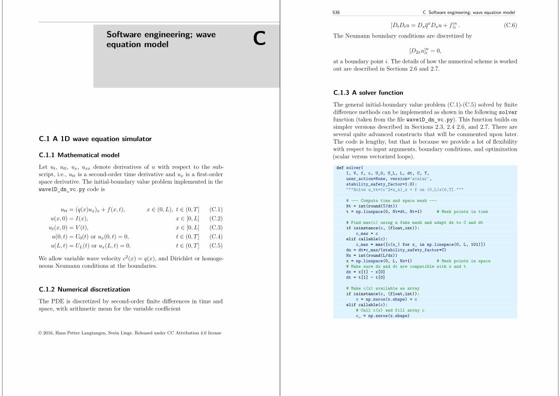
Software engineering; waveequation model C
C.1 A 1D wave equation simulator
C.1.1 Mathematical modelLet ut, utt, ux, uxx denote derivatives of u with respect to the sub-script, i.e., utt is a second-order time derivative and ux is a first-orderspace derivative. The initial-boundary value problem implemented in thewave1D_dn_vc.py code is
utt = (q(x)ux)x + f(x, t), x ∈ (0, L), t ∈ (0, T ] (C.1)u(x, 0) = I(x), x ∈ [0, L] (C.2)ut(x, 0) = V (t), x ∈ [0, L] (C.3)u(0, t) = U0(t) or ux(0, t) = 0, t ∈ (0, T ] (C.4)u(L, t) = UL(t) or ux(L, t) = 0, t ∈ (0, T ] (C.5)
We allow variable wave velocity c2(x) = q(x), and Dirichlet or homoge-neous Neumann conditions at the boundaries.
C.1.2 Numerical discretizationThe PDE is discretized by second-order finite differences in time andspace, with arithmetic mean for the variable coefficient
© 2016, Hans Petter Langtangen, Svein Linge. Released under CC Attribution 4.0 license
536 C Software engineering; wave equation model
[DtDtu = DxqxDxu+ f ]ni . (C.6)
The Neumann boundary conditions are discretized by
[D2xu]ni = 0,
at a boundary point i. The details of how the numerical scheme is workedout are described in Sections 2.6 and 2.7.
C.1.3 A solver function
The general initial-boundary value problem (C.1)-(C.5) solved by finitedifference methods can be implemented as shown in the following solverfunction (taken from the file wave1D_dn_vc.py). This function builds onsimpler versions described in Sections 2.3, 2.4 2.6, and 2.7. There areseveral quite advanced constructs that will be commented upon later.The code is lengthy, but that is because we provide a lot of flexibilitywith respect to input arguments, boundary conditions, and optimization(scalar versus vectorized loops).
def solver(I, V, f, c, U_0, U_L, L, dt, C, T,user_action=None, version=’scalar’,stability_safety_factor=1.0):"""Solve u_tt=(c^2*u_x)_x + f on (0,L)x(0,T]."""
# --- Compute time and space mesh ---Nt = int(round(T/dt))t = np.linspace(0, Nt*dt, Nt+1) # Mesh points in time
# Find max(c) using a fake mesh and adapt dx to C and dtif isinstance(c, (float,int)):
c_max = celif callable(c):
c_max = max([c(x_) for x_ in np.linspace(0, L, 101)])dx = dt*c_max/(stability_safety_factor*C)Nx = int(round(L/dx))x = np.linspace(0, L, Nx+1) # Mesh points in space# Make sure dx and dt are compatible with x and tdx = x[1] - x[0]dt = t[1] - t[0]
# Make c(x) available as arrayif isinstance(c, (float,int)):
c = np.zeros(x.shape) + celif callable(c):
# Call c(x) and fill array cc_ = np.zeros(x.shape)
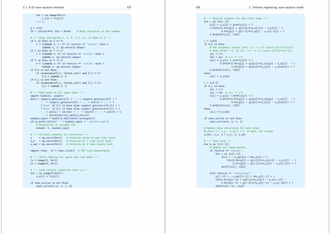
C.1 A 1D wave equation simulator 537
for i in range(Nx+1):c_[i] = c(x[i])
c = c_
q = c**2C2 = (dt/dx)**2; dt2 = dt*dt # Help variables in the scheme
# --- Wrap user-given f, I, V, U_0, U_L if None or 0 ---if f is None or f == 0:
f = (lambda x, t: 0) if version == ’scalar’ else \lambda x, t: np.zeros(x.shape)
if I is None or I == 0:I = (lambda x: 0) if version == ’scalar’ else \
lambda x: np.zeros(x.shape)if V is None or V == 0:
V = (lambda x: 0) if version == ’scalar’ else \lambda x: np.zeros(x.shape)
if U_0 is not None:if isinstance(U_0, (float,int)) and U_0 == 0:
U_0 = lambda t: 0if U_L is not None:
if isinstance(U_L, (float,int)) and U_L == 0:U_L = lambda t: 0
# --- Make hash of all input data ---import hashlib, inspectdata = inspect.getsource(I) + ’_’ + inspect.getsource(V) + \
’_’ + inspect.getsource(f) + ’_’ + str(c) + ’_’ + \(’None’ if U_0 is None else inspect.getsource(U_0)) + \(’None’ if U_L is None else inspect.getsource(U_L)) + \’_’ + str(L) + str(dt) + ’_’ + str(C) + ’_’ + str(T) + \’_’ + str(stability_safety_factor)
hashed_input = hashlib.sha1(data).hexdigest()if os.path.isfile(’.’ + hashed_input + ’_archive.npz’):
# Simulation is already runreturn -1, hashed_input
# --- Allocate memomry for solutions ---u = np.zeros(Nx+1) # Solution array at new time levelu_n = np.zeros(Nx+1) # Solution at 1 time level backu_nm1 = np.zeros(Nx+1) # Solution at 2 time levels back
import time; t0 = time.clock() # CPU time measurement
# --- Valid indices for space and time mesh ---Ix = range(0, Nx+1)It = range(0, Nt+1)
# --- Load initial condition into u_n ---for i in range(0,Nx+1):
u_n[i] = I(x[i])
if user_action is not None:user_action(u_n, x, t, 0)
538 C Software engineering; wave equation model
# --- Special formula for the first step ---for i in Ix[1:-1]:
u[i] = u_n[i] + dt*V(x[i]) + \0.5*C2*(0.5*(q[i] + q[i+1])*(u_n[i+1] - u_n[i]) - \
0.5*(q[i] + q[i-1])*(u_n[i] - u_n[i-1])) + \0.5*dt2*f(x[i], t[0])
i = Ix[0]if U_0 is None:
# Set boundary values (x=0: i-1 -> i+1 since u[i-1]=u[i+1]# when du/dn = 0, on x=L: i+1 -> i-1 since u[i+1]=u[i-1])ip1 = i+1im1 = ip1 # i-1 -> i+1u[i] = u_n[i] + dt*V(x[i]) + \
0.5*C2*(0.5*(q[i] + q[ip1])*(u_n[ip1] - u_n[i]) - \0.5*(q[i] + q[im1])*(u_n[i] - u_n[im1])) + \
0.5*dt2*f(x[i], t[0])else:
u[i] = U_0(dt)
i = Ix[-1]if U_L is None:
im1 = i-1ip1 = im1 # i+1 -> i-1u[i] = u_n[i] + dt*V(x[i]) + \
0.5*C2*(0.5*(q[i] + q[ip1])*(u_n[ip1] - u_n[i]) - \0.5*(q[i] + q[im1])*(u_n[i] - u_n[im1])) + \
0.5*dt2*f(x[i], t[0])else:
u[i] = U_L(dt)
if user_action is not None:user_action(u, x, t, 1)
# Update data structures for next step#u_nm1[:] = u_n; u_n[:] = u # safe, but sloweru_nm1, u_n, u = u_n, u, u_nm1
# --- Time loop ---for n in It[1:-1]:
# Update all inner pointsif version == ’scalar’:
for i in Ix[1:-1]:u[i] = - u_nm1[i] + 2*u_n[i] + \
C2*(0.5*(q[i] + q[i+1])*(u_n[i+1] - u_n[i]) - \0.5*(q[i] + q[i-1])*(u_n[i] - u_n[i-1])) + \
dt2*f(x[i], t[n])
elif version == ’vectorized’:u[1:-1] = - u_nm1[1:-1] + 2*u_n[1:-1] + \C2*(0.5*(q[1:-1] + q[2:])*(u_n[2:] - u_n[1:-1]) -
0.5*(q[1:-1] + q[:-2])*(u_n[1:-1] - u_n[:-2])) + \dt2*f(x[1:-1], t[n])
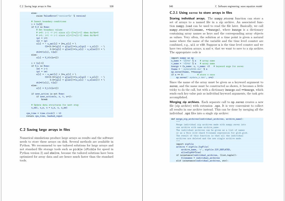
C.2 Saving large arrays in files 539
else:raise ValueError(’version=%s’ % version)
# Insert boundary conditionsi = Ix[0]if U_0 is None:
# Set boundary values# x=0: i-1 -> i+1 since u[i-1]=u[i+1] when du/dn=0# x=L: i+1 -> i-1 since u[i+1]=u[i-1] when du/dn=0ip1 = i+1im1 = ip1u[i] = - u_nm1[i] + 2*u_n[i] + \
C2*(0.5*(q[i] + q[ip1])*(u_n[ip1] - u_n[i]) - \0.5*(q[i] + q[im1])*(u_n[i] - u_n[im1])) + \
dt2*f(x[i], t[n])else:
u[i] = U_0(t[n+1])
i = Ix[-1]if U_L is None:
im1 = i-1ip1 = im1u[i] = - u_nm1[i] + 2*u_n[i] + \
C2*(0.5*(q[i] + q[ip1])*(u_n[ip1] - u_n[i]) - \0.5*(q[i] + q[im1])*(u_n[i] - u_n[im1])) + \
dt2*f(x[i], t[n])else:
u[i] = U_L(t[n+1])
if user_action is not None:if user_action(u, x, t, n+1):
break
# Update data structures for next stepu_nm1, u_n, u = u_n, u, u_nm1
cpu_time = time.clock() - t0return cpu_time, hashed_input
C.2 Saving large arrays in files
Numerical simulations produce large arrays as results and the softwareneeds to store these arrays on disk. Several methods are available inPython. We recommend to use tailored solutions for large arrays andnot standard file storage tools such as pickle (cPickle for speed inPython version 2) and shelve, because the tailored solutions have beenoptimized for array data and are hence much faster than the standardtools.
540 C Software engineering; wave equation model
C.2.1 Using savez to store arrays in filesStoring individual arrays. The numpy.storez function can store aset of arrays to a named file in a zip archive. An associated func-tion numpy.load can be used to read the file later. Basically, we callnumpy.storez(filename, **kwargs), where kwargs is a dictionarycontaining array names as keys and the corresponding array objectsas values. Very often, the solution at a time point is given a naturalname where the name of the variable and the time level counter arecombined, e.g., u11 or v39. Suppose n is the time level counter and wehave two solution arrays, u and v, that we want to save to a zip archive.The appropriate code is
import numpy as npu_name = ’u%04d’ % n # array namev_name = ’v%04d’ % n # array namekwargs = u_name: u, v_name: v # keyword args for savezfname = ’.mydata%04d.dat’ % nnp.savez(fname, **kwargs)if n == 0: # store x once
np.savez(’.mydata_x.dat’, x=x)
Since the name of the array must be given as a keyword argument tosavez, and the name must be constructed as shown, it becomes a littletricky to do the call, but with a dictionary kwargs and **kwargs, whichsends each key-value pair as individual keyword arguments, the task getsaccomplished.Merging zip archives. Each separate call to np.savez creates a newfile (zip archive) with extension .npz. It is very convenient to collectall results in one archive instead. This can be done by merging all theindividual .npz files into a single zip archive:
def merge_zip_archives(individual_archives, archive_name):"""Merge individual zip archives made with numpy.savez intoone archive with name archive_name.The individual archives can be given as a list of namesor as a Unix wild chard filename expression for glob.glob.The result of this function is that all the individualarchives are deleted and the new single archive made."""import zipfilearchive = zipfile.ZipFile(
archive_name, ’w’, zipfile.ZIP_DEFLATED,allowZip64=True)
if isinstance(individual_archives, (list,tuple)):filenames = individual_archives
elif isinstance(individual_archives, str):
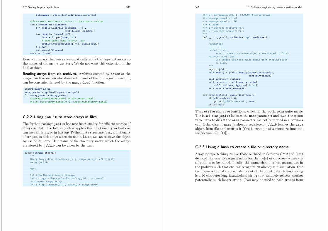
C.2 Saving large arrays in files 541
filenames = glob.glob(individual_archives)
# Open each archive and write to the common archivefor filename in filenames:
f = zipfile.ZipFile(filename, ’r’,zipfile.ZIP_DEFLATED)
for name in f.namelist():data = f.open(name, ’r’)# Save under name without .npyarchive.writestr(name[:-4], data.read())
f.close()os.remove(filename)
archive.close()
Here we remark that savez automatically adds the .npz extension tothe names of the arrays we store. We do not want this extension in thefinal archive.Reading arrays from zip archives. Archives created by savez or themerged archive we describe above with name of the form myarchive.npz,can be conveniently read by the numpy.load function:
import numpy as nparray_names = np.load(‘myarchive.npz‘)for array_name in array_names:
# array_names[array_name] is the array itself# e.g. plot(array_names[’t’], array_names[array_name])
C.2.2 Using joblib to store arrays in filesThe Python package joblib has nice functionality for efficient storage ofarrays on disk. The following class applies this functionality so that onecan save an array, or in fact any Python data structure (e.g., a dictionaryof arrays), to disk under a certain name. Later, we can retrieve the objectby use of its name. The name of the directory under which the arraysare stored by joblib can be given by the user.
class Storage(object):"""Store large data structures (e.g. numpy arrays) efficientlyusing joblib.
Use:
>>> from Storage import Storage>>> storage = Storage(cachedir=’tmp_u01’, verbose=1)>>> import numpy as np>>> a = np.linspace(0, 1, 100000) # large array
542 C Software engineering; wave equation model
>>> b = np.linspace(0, 1, 100000) # large array>>> storage.save(’a’, a)>>> storage.save(’b’, b)>>> # later>>> a = storage.retrieve(’a’)>>> b = storage.retrieve(’b’)"""def __init__(self, cachedir=’tmp’, verbose=1):
"""Parameters----------cachedir: str
Name of directory where objects are stored in files.verbose: bool, int
Let joblib and this class speak when storing filesto disk.
"""import joblibself.memory = joblib.Memory(cachedir=cachedir,
verbose=verbose)self.verbose = verboseself.retrieve = self.memory.cache(
self.retrieve, ignore=[’data’])self.save = self.retrieve
def retrieve(self, name, data=None):if self.verbose > 0:
print ’joblib save of’, namereturn data
The retrive and save functions, which do the work, seem quite magic.The idea is that joblib looks at the name parameter and saves the returnvalue data to disk if the name parameter has not been used in a previouscall. Otherwise, if name is already registered, joblib fetches the dataobject from file and returns it (this is example of a memoize function,see Section ??in [11]).
C.2.3 Using a hash to create a file or directory name
Array storage techniques like those outlined in Sections C.2.2 and C.2.1demand the user to assign a name for the file(s) or directory where thesolution is to be stored. Ideally, this name should reflect parameters inthe problem such that one can recognize an already run simulation. Onetechnique is to make a hash string out of the input data. A hash stringis a 40-character long hexadecimal string that uniquely reflects anotherpotentially much longer string. (You may be used to hash strings from
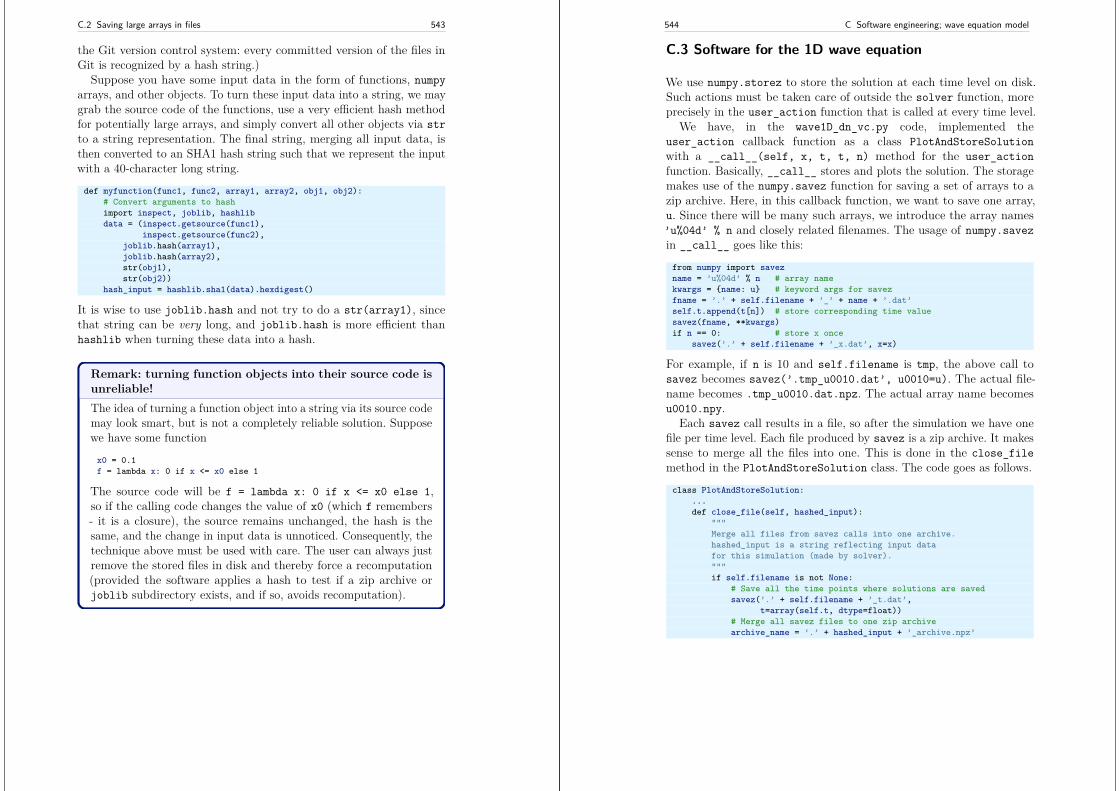
C.2 Saving large arrays in files 543
the Git version control system: every committed version of the files inGit is recognized by a hash string.)
Suppose you have some input data in the form of functions, numpyarrays, and other objects. To turn these input data into a string, we maygrab the source code of the functions, use a very efficient hash methodfor potentially large arrays, and simply convert all other objects via strto a string representation. The final string, merging all input data, isthen converted to an SHA1 hash string such that we represent the inputwith a 40-character long string.
def myfunction(func1, func2, array1, array2, obj1, obj2):# Convert arguments to hashimport inspect, joblib, hashlibdata = (inspect.getsource(func1),
inspect.getsource(func2),joblib.hash(array1),joblib.hash(array2),str(obj1),str(obj2))
hash_input = hashlib.sha1(data).hexdigest()
It is wise to use joblib.hash and not try to do a str(array1), sincethat string can be very long, and joblib.hash is more efficient thanhashlib when turning these data into a hash.
Remark: turning function objects into their source code isunreliable!The idea of turning a function object into a string via its source codemay look smart, but is not a completely reliable solution. Supposewe have some function
x0 = 0.1f = lambda x: 0 if x <= x0 else 1
The source code will be f = lambda x: 0 if x <= x0 else 1,so if the calling code changes the value of x0 (which f remembers- it is a closure), the source remains unchanged, the hash is thesame, and the change in input data is unnoticed. Consequently, thetechnique above must be used with care. The user can always justremove the stored files in disk and thereby force a recomputation(provided the software applies a hash to test if a zip archive orjoblib subdirectory exists, and if so, avoids recomputation).
544 C Software engineering; wave equation model
C.3 Software for the 1D wave equation
We use numpy.storez to store the solution at each time level on disk.Such actions must be taken care of outside the solver function, moreprecisely in the user_action function that is called at every time level.
We have, in the wave1D_dn_vc.py code, implemented theuser_action callback function as a class PlotAndStoreSolutionwith a __call__(self, x, t, t, n) method for the user_actionfunction. Basically, __call__ stores and plots the solution. The storagemakes use of the numpy.savez function for saving a set of arrays to azip archive. Here, in this callback function, we want to save one array,u. Since there will be many such arrays, we introduce the array names’u%04d’ % n and closely related filenames. The usage of numpy.savezin __call__ goes like this:
from numpy import savezname = ’u%04d’ % n # array namekwargs = name: u # keyword args for savezfname = ’.’ + self.filename + ’_’ + name + ’.dat’self.t.append(t[n]) # store corresponding time valuesavez(fname, **kwargs)if n == 0: # store x once
savez(’.’ + self.filename + ’_x.dat’, x=x)
For example, if n is 10 and self.filename is tmp, the above call tosavez becomes savez(’.tmp_u0010.dat’, u0010=u). The actual file-name becomes .tmp_u0010.dat.npz. The actual array name becomesu0010.npy.
Each savez call results in a file, so after the simulation we have onefile per time level. Each file produced by savez is a zip archive. It makessense to merge all the files into one. This is done in the close_filemethod in the PlotAndStoreSolution class. The code goes as follows.
class PlotAndStoreSolution:...def close_file(self, hashed_input):
"""Merge all files from savez calls into one archive.hashed_input is a string reflecting input datafor this simulation (made by solver)."""if self.filename is not None:
# Save all the time points where solutions are savedsavez(’.’ + self.filename + ’_t.dat’,
t=array(self.t, dtype=float))# Merge all savez files to one zip archivearchive_name = ’.’ + hashed_input + ’_archive.npz’
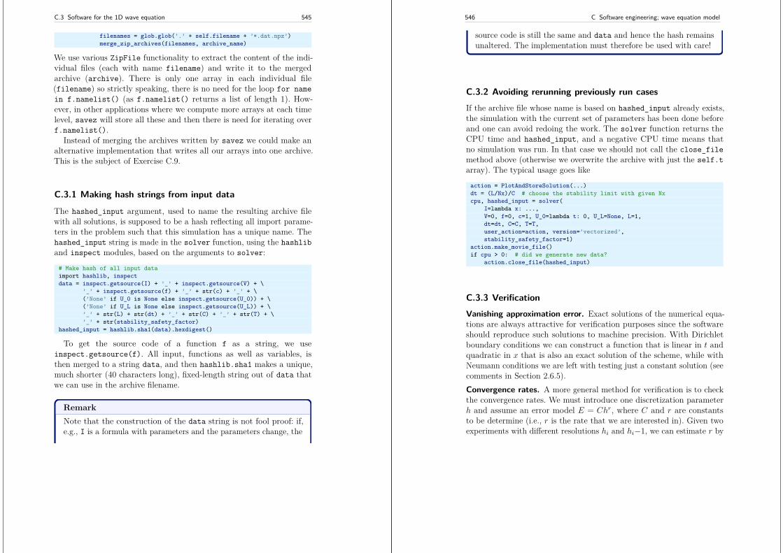
C.3 Software for the 1D wave equation 545
filenames = glob.glob(’.’ + self.filename + ’*.dat.npz’)merge_zip_archives(filenames, archive_name)
We use various ZipFile functionality to extract the content of the indi-vidual files (each with name filename) and write it to the mergedarchive (archive). There is only one array in each individual file(filename) so strictly speaking, there is no need for the loop for namein f.namelist() (as f.namelist() returns a list of length 1). How-ever, in other applications where we compute more arrays at each timelevel, savez will store all these and then there is need for iterating overf.namelist().
Instead of merging the archives written by savez we could make analternative implementation that writes all our arrays into one archive.This is the subject of Exercise C.9.
C.3.1 Making hash strings from input data
The hashed_input argument, used to name the resulting archive filewith all solutions, is supposed to be a hash reflecting all import parame-ters in the problem such that this simulation has a unique name. Thehashed_input string is made in the solver function, using the hashliband inspect modules, based on the arguments to solver:
# Make hash of all input dataimport hashlib, inspectdata = inspect.getsource(I) + ’_’ + inspect.getsource(V) + \
’_’ + inspect.getsource(f) + ’_’ + str(c) + ’_’ + \(’None’ if U_0 is None else inspect.getsource(U_0)) + \(’None’ if U_L is None else inspect.getsource(U_L)) + \’_’ + str(L) + str(dt) + ’_’ + str(C) + ’_’ + str(T) + \’_’ + str(stability_safety_factor)
hashed_input = hashlib.sha1(data).hexdigest()
To get the source code of a function f as a string, we useinspect.getsource(f). All input, functions as well as variables, isthen merged to a string data, and then hashlib.sha1 makes a unique,much shorter (40 characters long), fixed-length string out of data thatwe can use in the archive filename.
RemarkNote that the construction of the data string is not fool proof: if,e.g., I is a formula with parameters and the parameters change, the
546 C Software engineering; wave equation model
source code is still the same and data and hence the hash remainsunaltered. The implementation must therefore be used with care!
C.3.2 Avoiding rerunning previously run casesIf the archive file whose name is based on hashed_input already exists,the simulation with the current set of parameters has been done beforeand one can avoid redoing the work. The solver function returns theCPU time and hashed_input, and a negative CPU time means thatno simulation was run. In that case we should not call the close_filemethod above (otherwise we overwrite the archive with just the self.tarray). The typical usage goes like
action = PlotAndStoreSolution(...)dt = (L/Nx)/C # choose the stability limit with given Nxcpu, hashed_input = solver(
I=lambda x: ...,V=0, f=0, c=1, U_0=lambda t: 0, U_L=None, L=1,dt=dt, C=C, T=T,user_action=action, version=’vectorized’,stability_safety_factor=1)
action.make_movie_file()if cpu > 0: # did we generate new data?
action.close_file(hashed_input)
C.3.3 VerificationVanishing approximation error. Exact solutions of the numerical equa-tions are always attractive for verification purposes since the softwareshould reproduce such solutions to machine precision. With Dirichletboundary conditions we can construct a function that is linear in t andquadratic in x that is also an exact solution of the scheme, while withNeumann conditions we are left with testing just a constant solution (seecomments in Section 2.6.5).Convergence rates. A more general method for verification is to checkthe convergence rates. We must introduce one discretization parameterh and assume an error model E = Chr, where C and r are constantsto be determine (i.e., r is the rate that we are interested in). Given twoexperiments with different resolutions hi and hi−1, we can estimate r by
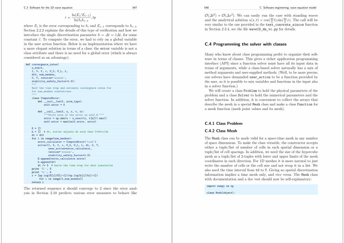
C.3 Software for the 1D wave equation 547
r = ln(Ei/Ei−1)ln(hihi−1
, tp
where Ei is the error corresponding to hi and Ei−1 corresponds to hi−1.Section 2.2.2 explains the details of this type of verification and how weintroduce the single discretization parameter h = ∆t = c∆t, for someconstant c. To compute the error, we had to rely on a global variablein the user action function. Below is an implementation where we havea more elegant solution in terms of a class: the error variable is not aclass attribute and there is no need for a global error (which is alwaysconsidered as an advantage).
def convergence_rates(u_exact,I, V, f, c, U_0, U_L, L,dt0, num_meshes,C, T, version=’scalar’,stability_safety_factor=1.0):"""Half the time step and estimate convergence rates forfor num_meshes simulations."""class ComputeError:
def __init__(self, norm_type):self.error = 0
def __call__(self, u, x, t, n):"""Store norm of the error in self.E."""error = np.abs(u - u_exact(x, t[n])).max()self.error = max(self.error, error)
E = []h = [] # dt, solver adjusts dx such that C=dt*c/dxdt = dt0for i in range(num_meshes):
error_calculator = ComputeError(’Linf’)solver(I, V, f, c, U_0, U_L, L, dt, C, T,
user_action=error_calculator,version=’scalar’,stability_safety_factor=1.0)
E.append(error_calculator.error)h.append(dt)dt /= 2 # halve the time step for next simulation
print ’E:’, Eprint ’h:’, hr = [np.log(E[i]/E[i-1])/np.log(h[i]/h[i-1])
for i in range(1,num_meshes)]return r
The returned sequence r should converge to 2 since the error anal-ysis in Section 2.10 predicts various error measures to behave like
548 C Software engineering; wave equation model
O(∆t2) + O(∆x2). We can easily run the case with standing wavesand the analytical solution u(x, t) = cos(2π
L t) sin(2πL x). The call will be
very similar to the one provided in the test_convrate_sincos functionin Section 2.3.4, see the file wave1D_dn_vc.py for details.
C.4 Programming the solver with classes
Many who know about class programming prefer to organize their soft-ware in terms of classes. This gives a richer application programminginterface (API) since a function solver must have all its input data interms of arguments, while a class-based solver naturally has a mix ofmethod arguments and user-supplied methods. (Well, to be more precise,our solvers have demanded user_action to be a function provided bythe user, so it is possible to mix variables and functions in the input alsoin a solver function.)
We will create a class Problem to hold the physical parameters of theproblem and a class Solver to hold the numerical parameters and thesolver function. In addition, it is convenient to collect the arrays thatdescribe the mesh in a special Mesh class and make a class Function fora mesh function (mesh point values and its mesh).
C.4.1 Class Problem
C.4.2 Class Mesh
The Mesh class can be made valid for a space-time mesh in any numberof space dimensions. To make the class versatile, the constructor acceptseither a tuple/list of number of cells in each spatial dimension or atuple/list of cell spacings. In addition, we need the size of the hypercubemesh as a tuple/list of 2-tuples with lower and upper limits of the meshcoordinates in each direction. For 1D meshes it is more natural to justwrite the number of cells or the cell size and not wrap it in a list. Wealso need the time interval from t0 to T. Giving no spatial discretizationinformation implies a time mesh only, and vice versa. The Mesh classwith documentation and a doc test should now be self-explanatory:
import numpy as np
class Mesh(object):
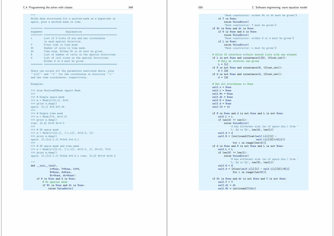
C.4 Programming the solver with classes 549
"""Holds data structures for a uniform mesh on a hypercube inspace, plus a uniform mesh in time.
======== ==================================================Argument Explanation======== ==================================================L List of 2-lists of min and max coordinates
in each spatial direction.T Final time in time mesh.Nt Number of cells in time mesh.dt Time step. Either Nt or dt must be given.N List of number of cells in the spatial directions.d List of cell sizes in the spatial directions.
Either N or d must be given.======== ==================================================
Users can access all the parameters mentioned above, plus‘‘x[i]‘‘ and ‘‘t‘‘ for the coordinates in direction ‘‘i‘‘and the time coordinates, respectively.
Examples:
>>> from UniformFDMesh import Mesh>>>>>> # Simple space mesh>>> m = Mesh(L=[0,1], N=4)>>> print m.dump()space: [0,1] N=4 d=0.25>>>>>> # Simple time mesh>>> m = Mesh(T=4, dt=0.5)>>> print m.dump()time: [0,4] Nt=8 dt=0.5>>>>>> # 2D space mesh>>> m = Mesh(L=[[0,1], [-1,1]], d=[0.5, 1])>>> print m.dump()space: [0,1]x[-1,1] N=2x2 d=0.5,1>>>>>> # 2D space mesh and time mesh>>> m = Mesh(L=[[0,1], [-1,1]], d=[0.5, 1], Nt=10, T=3)>>> print m.dump()space: [0,1]x[-1,1] N=2x2 d=0.5,1 time: [0,3] Nt=10 dt=0.3
"""def __init__(self,
L=None, T=None, t0=0,N=None, d=None,Nt=None, dt=None):
if N is None and d is None:# No spatial meshif Nt is None and dt is None:
raise ValueError(
550 C Software engineering; wave equation model
’Mesh constructor: either Nt or dt must be given’)if T is None:
raise ValueError(’Mesh constructor: T must be given’)
if Nt is None and dt is None:if N is None and d is None:
raise ValueError(’Mesh constructor: either N or d must be given’)
if L is None:raise ValueError(’Mesh constructor: L must be given’)
# Allow 1D interface without nested lists with one elementif L is not None and isinstance(L[0], (float,int)):
# Only an interval was givenL = [L]
if N is not None and isinstance(N, (float,int)):N = [N]
if d is not None and isinstance(d, (float,int)):d = [d]
# Set all attributes to Noneself.x = Noneself.t = Noneself.Nt = Noneself.dt = Noneself.N = Noneself.d = Noneself.t0 = t0
if N is None and d is not None and L is not None:self.L = Lif len(d) != len(L):
raise ValueError(’d has different size (no of space dim.) from ’’L: %d vs %d’, len(d), len(L))
self.d = dself.N = [int(round(float(self.L[i][1] -
self.L[i][0])/d[i]))for i in range(len(d))]
if d is None and N is not None and L is not None:self.L = Lif len(N) != len(L):
raise ValueError(’N has different size (no of space dim.) from ’’L: %d vs %d’, len(N), len(L))
self.N = Nself.d = [float(self.L[i][1] - self.L[i][0])/N[i]
for i in range(len(N))]
if Nt is None and dt is not None and T is not None:self.T = Tself.dt = dtself.Nt = int(round(T/dt))
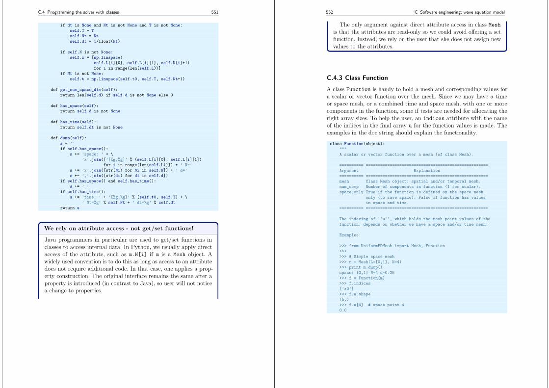
C.4 Programming the solver with classes 551
if dt is None and Nt is not None and T is not None:self.T = Tself.Nt = Ntself.dt = T/float(Nt)
if self.N is not None:self.x = [np.linspace(
self.L[i][0], self.L[i][1], self.N[i]+1)for i in range(len(self.L))]
if Nt is not None:self.t = np.linspace(self.t0, self.T, self.Nt+1)
def get_num_space_dim(self):return len(self.d) if self.d is not None else 0
def has_space(self):return self.d is not None
def has_time(self):return self.dt is not None
def dump(self):s = ’’if self.has_space():
s += ’space: ’ + \’x’.join([’[%g,%g]’ % (self.L[i][0], self.L[i][1])
for i in range(len(self.L))]) + ’ N=’s += ’x’.join([str(Ni) for Ni in self.N]) + ’ d=’s += ’,’.join([str(di) for di in self.d])
if self.has_space() and self.has_time():s += ’ ’
if self.has_time():s += ’time: ’ + ’[%g,%g]’ % (self.t0, self.T) + \
’ Nt=%g’ % self.Nt + ’ dt=%g’ % self.dtreturn s
We rely on attribute access - not get/set functions!
Java programmers in particular are used to get/set functions inclasses to access internal data. In Python, we usually apply directaccess of the attribute, such as m.N[i] if m is a Mesh object. Awidely used convention is to do this as long as access to an attributedoes not require additional code. In that case, one applies a prop-erty construction. The original interface remains the same after aproperty is introduced (in contrast to Java), so user will not noticea change to properties.
552 C Software engineering; wave equation model
The only argument against direct attribute access in class Meshis that the attributes are read-only so we could avoid offering a setfunction. Instead, we rely on the user that she does not assign newvalues to the attributes.
C.4.3 Class FunctionA class Function is handy to hold a mesh and corresponding values fora scalar or vector function over the mesh. Since we may have a timeor space mesh, or a combined time and space mesh, with one or morecomponents in the function, some if tests are needed for allocating theright array sizes. To help the user, an indices attribute with the nameof the indices in the final array u for the function values is made. Theexamples in the doc string should explain the functionality.
class Function(object):"""A scalar or vector function over a mesh (of class Mesh).
========== ===================================================Argument Explanation========== ===================================================mesh Class Mesh object: spatial and/or temporal mesh.num_comp Number of components in function (1 for scalar).space_only True if the function is defined on the space mesh
only (to save space). False if function has valuesin space and time.
========== ===================================================
The indexing of ‘‘u‘‘, which holds the mesh point values of thefunction, depends on whether we have a space and/or time mesh.
Examples:
>>> from UniformFDMesh import Mesh, Function>>>>>> # Simple space mesh>>> m = Mesh(L=[0,1], N=4)>>> print m.dump()space: [0,1] N=4 d=0.25>>> f = Function(m)>>> f.indices[’x0’]>>> f.u.shape(5,)>>> f.u[4] # space point 40.0
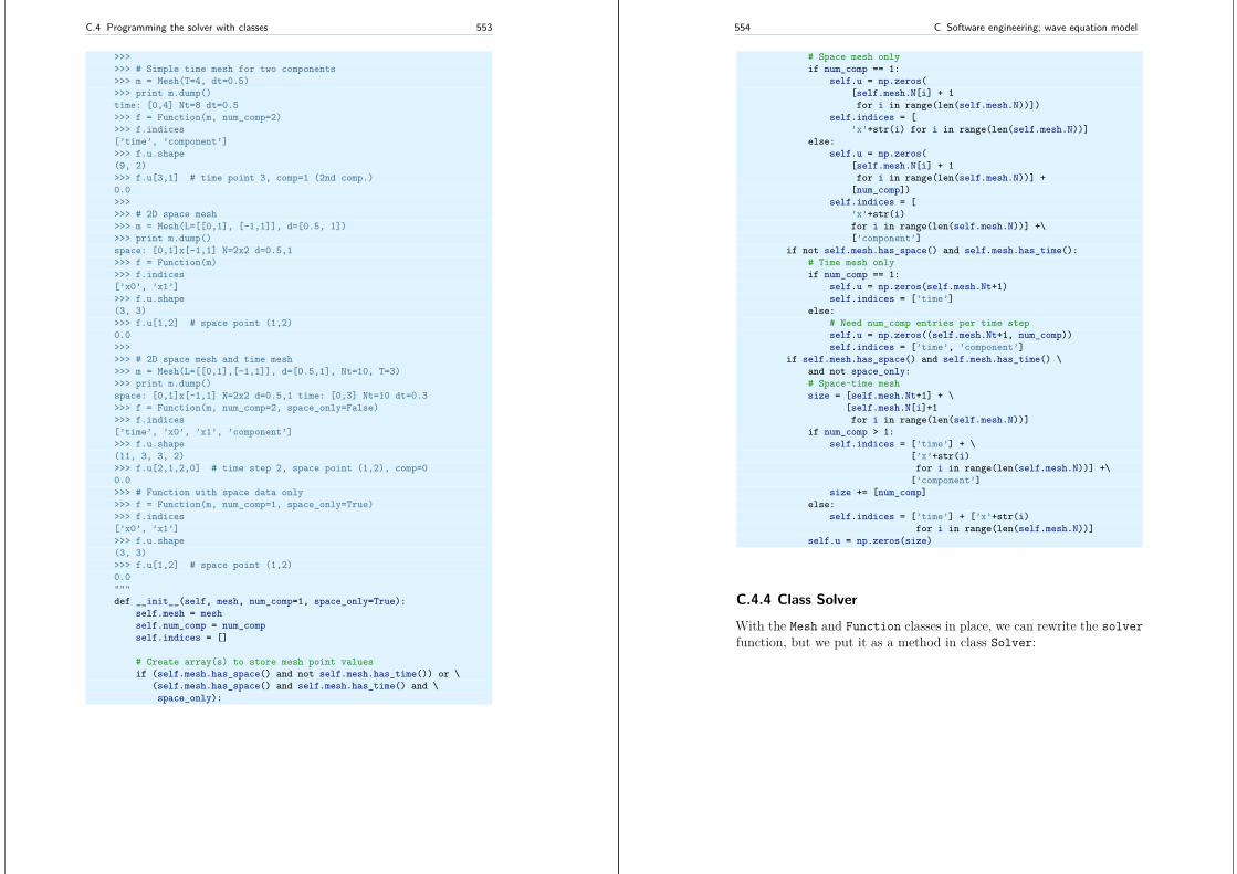
C.4 Programming the solver with classes 553
>>>>>> # Simple time mesh for two components>>> m = Mesh(T=4, dt=0.5)>>> print m.dump()time: [0,4] Nt=8 dt=0.5>>> f = Function(m, num_comp=2)>>> f.indices[’time’, ’component’]>>> f.u.shape(9, 2)>>> f.u[3,1] # time point 3, comp=1 (2nd comp.)0.0>>>>>> # 2D space mesh>>> m = Mesh(L=[[0,1], [-1,1]], d=[0.5, 1])>>> print m.dump()space: [0,1]x[-1,1] N=2x2 d=0.5,1>>> f = Function(m)>>> f.indices[’x0’, ’x1’]>>> f.u.shape(3, 3)>>> f.u[1,2] # space point (1,2)0.0>>>>>> # 2D space mesh and time mesh>>> m = Mesh(L=[[0,1],[-1,1]], d=[0.5,1], Nt=10, T=3)>>> print m.dump()space: [0,1]x[-1,1] N=2x2 d=0.5,1 time: [0,3] Nt=10 dt=0.3>>> f = Function(m, num_comp=2, space_only=False)>>> f.indices[’time’, ’x0’, ’x1’, ’component’]>>> f.u.shape(11, 3, 3, 2)>>> f.u[2,1,2,0] # time step 2, space point (1,2), comp=00.0>>> # Function with space data only>>> f = Function(m, num_comp=1, space_only=True)>>> f.indices[’x0’, ’x1’]>>> f.u.shape(3, 3)>>> f.u[1,2] # space point (1,2)0.0"""def __init__(self, mesh, num_comp=1, space_only=True):
self.mesh = meshself.num_comp = num_compself.indices = []
# Create array(s) to store mesh point valuesif (self.mesh.has_space() and not self.mesh.has_time()) or \
(self.mesh.has_space() and self.mesh.has_time() and \space_only):
554 C Software engineering; wave equation model
# Space mesh onlyif num_comp == 1:
self.u = np.zeros([self.mesh.N[i] + 1for i in range(len(self.mesh.N))])
self.indices = [’x’+str(i) for i in range(len(self.mesh.N))]
else:self.u = np.zeros(
[self.mesh.N[i] + 1for i in range(len(self.mesh.N))] +
[num_comp])self.indices = [
’x’+str(i)for i in range(len(self.mesh.N))] +\[’component’]
if not self.mesh.has_space() and self.mesh.has_time():# Time mesh onlyif num_comp == 1:
self.u = np.zeros(self.mesh.Nt+1)self.indices = [’time’]
else:# Need num_comp entries per time stepself.u = np.zeros((self.mesh.Nt+1, num_comp))self.indices = [’time’, ’component’]
if self.mesh.has_space() and self.mesh.has_time() \and not space_only:# Space-time meshsize = [self.mesh.Nt+1] + \
[self.mesh.N[i]+1for i in range(len(self.mesh.N))]
if num_comp > 1:self.indices = [’time’] + \
[’x’+str(i)for i in range(len(self.mesh.N))] +\
[’component’]size += [num_comp]
else:self.indices = [’time’] + [’x’+str(i)
for i in range(len(self.mesh.N))]self.u = np.zeros(size)
C.4.4 Class Solver
With the Mesh and Function classes in place, we can rewrite the solverfunction, but we put it as a method in class Solver:
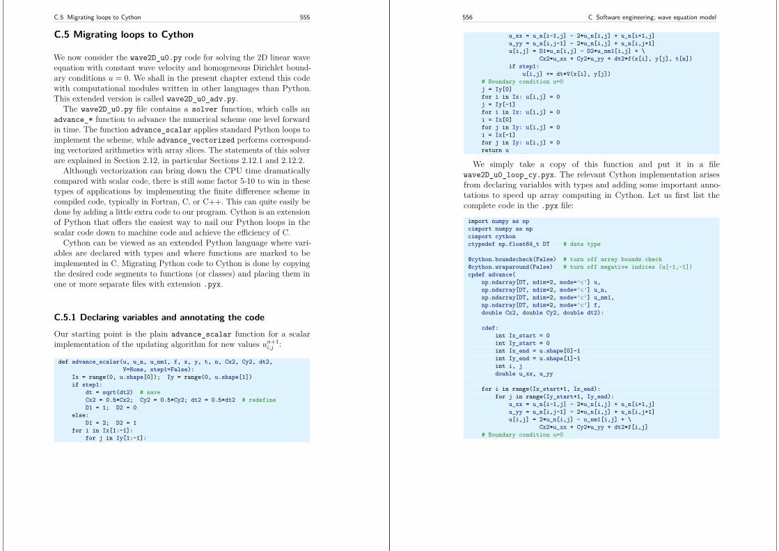
C.5 Migrating loops to Cython 555
C.5 Migrating loops to Cython
We now consider the wave2D_u0.py code for solving the 2D linear waveequation with constant wave velocity and homogeneous Dirichlet bound-ary conditions u = 0. We shall in the present chapter extend this codewith computational modules written in other languages than Python.This extended version is called wave2D_u0_adv.py.
The wave2D_u0.py file contains a solver function, which calls anadvance_* function to advance the numerical scheme one level forwardin time. The function advance_scalar applies standard Python loops toimplement the scheme, while advance_vectorized performs correspond-ing vectorized arithmetics with array slices. The statements of this solverare explained in Section 2.12, in particular Sections 2.12.1 and 2.12.2.
Although vectorization can bring down the CPU time dramaticallycompared with scalar code, there is still some factor 5-10 to win in thesetypes of applications by implementing the finite difference scheme incompiled code, typically in Fortran, C, or C++. This can quite easily bedone by adding a little extra code to our program. Cython is an extensionof Python that offers the easiest way to nail our Python loops in thescalar code down to machine code and achieve the efficiency of C.
Cython can be viewed as an extended Python language where vari-ables are declared with types and where functions are marked to beimplemented in C. Migrating Python code to Cython is done by copyingthe desired code segments to functions (or classes) and placing them inone or more separate files with extension .pyx.
C.5.1 Declaring variables and annotating the code
Our starting point is the plain advance_scalar function for a scalarimplementation of the updating algorithm for new values un+1
i,j :
def advance_scalar(u, u_n, u_nm1, f, x, y, t, n, Cx2, Cy2, dt2,V=None, step1=False):
Ix = range(0, u.shape[0]); Iy = range(0, u.shape[1])if step1:
dt = sqrt(dt2) # saveCx2 = 0.5*Cx2; Cy2 = 0.5*Cy2; dt2 = 0.5*dt2 # redefineD1 = 1; D2 = 0
else:D1 = 2; D2 = 1
for i in Ix[1:-1]:for j in Iy[1:-1]:
556 C Software engineering; wave equation model
u_xx = u_n[i-1,j] - 2*u_n[i,j] + u_n[i+1,j]u_yy = u_n[i,j-1] - 2*u_n[i,j] + u_n[i,j+1]u[i,j] = D1*u_n[i,j] - D2*u_nm1[i,j] + \
Cx2*u_xx + Cy2*u_yy + dt2*f(x[i], y[j], t[n])if step1:
u[i,j] += dt*V(x[i], y[j])# Boundary condition u=0j = Iy[0]for i in Ix: u[i,j] = 0j = Iy[-1]for i in Ix: u[i,j] = 0i = Ix[0]for j in Iy: u[i,j] = 0i = Ix[-1]for j in Iy: u[i,j] = 0return u
We simply take a copy of this function and put it in a filewave2D_u0_loop_cy.pyx. The relevant Cython implementation arisesfrom declaring variables with types and adding some important anno-tations to speed up array computing in Cython. Let us first list thecomplete code in the .pyx file:
import numpy as npcimport numpy as npcimport cythonctypedef np.float64_t DT # data type
@cython.boundscheck(False) # turn off array bounds [email protected](False) # turn off negative indices (u[-1,-1])cpdef advance(
np.ndarray[DT, ndim=2, mode=’c’] u,np.ndarray[DT, ndim=2, mode=’c’] u_n,np.ndarray[DT, ndim=2, mode=’c’] u_nm1,np.ndarray[DT, ndim=2, mode=’c’] f,double Cx2, double Cy2, double dt2):
cdef:int Ix_start = 0int Iy_start = 0int Ix_end = u.shape[0]-1int Iy_end = u.shape[1]-1int i, jdouble u_xx, u_yy
for i in range(Ix_start+1, Ix_end):for j in range(Iy_start+1, Iy_end):
u_xx = u_n[i-1,j] - 2*u_n[i,j] + u_n[i+1,j]u_yy = u_n[i,j-1] - 2*u_n[i,j] + u_n[i,j+1]u[i,j] = 2*u_n[i,j] - u_nm1[i,j] + \
Cx2*u_xx + Cy2*u_yy + dt2*f[i,j]# Boundary condition u=0
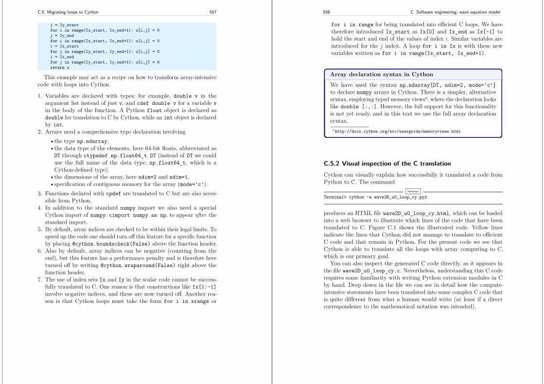
C.5 Migrating loops to Cython 557
j = Iy_startfor i in range(Ix_start, Ix_end+1): u[i,j] = 0j = Iy_endfor i in range(Ix_start, Ix_end+1): u[i,j] = 0i = Ix_startfor j in range(Iy_start, Iy_end+1): u[i,j] = 0i = Ix_endfor j in range(Iy_start, Iy_end+1): u[i,j] = 0return u
This example may act as a recipe on how to transform array-intensivecode with loops into Cython.
1. Variables are declared with types: for example, double v in theargument list instead of just v, and cdef double v for a variable vin the body of the function. A Python float object is declared asdouble for translation to C by Cython, while an int object is declaredby int.
2. Arrays need a comprehensive type declaration involving•the type np.ndarray,•the data type of the elements, here 64-bit floats, abbreviated asDT through ctypedef np.float64_t DT (instead of DT we coulduse the full name of the data type: np.float64_t, which is aCython-defined type),
•the dimensions of the array, here ndim=2 and ndim=1,•specification of contiguous memory for the array (mode=’c’).
3. Functions declared with cpdef are translated to C but are also acces-sible from Python.
4. In addition to the standard numpy import we also need a specialCython import of numpy: cimport numpy as np, to appear after thestandard import.
5. By default, array indices are checked to be within their legal limits. Tospeed up the code one should turn off this feature for a specific functionby placing @cython.boundscheck(False) above the function header.
6. Also by default, array indices can be negative (counting from theend), but this feature has a performance penalty and is therefore hereturned off by writing @cython.wraparound(False) right above thefunction header.
7. The use of index sets Ix and Iy in the scalar code cannot be success-fully translated to C. One reason is that constructions like Ix[1:-1]involve negative indices, and these are now turned off. Another rea-son is that Cython loops must take the form for i in xrange or
558 C Software engineering; wave equation model
for i in range for being translated into efficient C loops. We havetherefore introduced Ix_start as Ix[0] and Ix_end as Ix[-1] tohold the start and end of the values of index i. Similar variables areintroduced for the j index. A loop for i in Ix is with these newvariables written as for i in range(Ix_start, Ix_end+1).
Array declaration syntax in Cython
We have used the syntax np.ndarray[DT, ndim=2, mode=’c’]to declare numpy arrays in Cython. There is a simpler, alternativesyntax, employing typed memory viewsa, where the declaration lookslike double [:,:]. However, the full support for this functionalityis not yet ready, and in this text we use the full array declarationsyntax.
a http://docs.cython.org/src/userguide/memoryviews.html
C.5.2 Visual inspection of the C translationCython can visually explain how successfully it translated a code fromPython to C. The command
Terminal
Terminal> cython -a wave2D_u0_loop_cy.pyx
produces an HTML file wave2D_u0_loop_cy.html, which can be loadedinto a web browser to illustrate which lines of the code that have beentranslated to C. Figure C.1 shows the illustrated code. Yellow linesindicate the lines that Cython did not manage to translate to efficientC code and that remain in Python. For the present code we see thatCython is able to translate all the loops with array computing to C,which is our primary goal.
You can also inspect the generated C code directly, as it appears inthe file wave2D_u0_loop_cy.c. Nevertheless, understanding this C coderequires some familiarity with writing Python extension modules in Cby hand. Deep down in the file we can see in detail how the compute-intensive statements have been translated into some complex C code thatis quite different from what a human would write (at least if a directcorrespondence to the mathematical notation was intended).
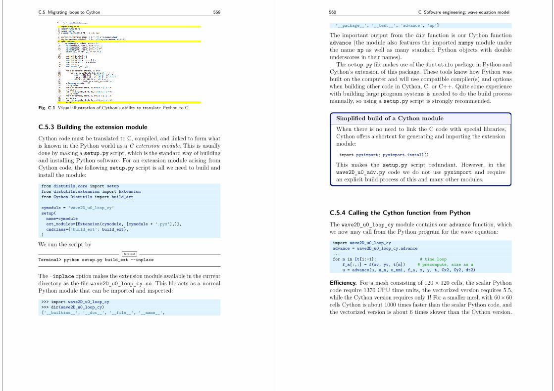
C.5 Migrating loops to Cython 559
Fig. C.1 Visual illustration of Cython’s ability to translate Python to C.
C.5.3 Building the extension moduleCython code must be translated to C, compiled, and linked to form whatis known in the Python world as a C extension module. This is usuallydone by making a setup.py script, which is the standard way of buildingand installing Python software. For an extension module arising fromCython code, the following setup.py script is all we need to build andinstall the module:
from distutils.core import setupfrom distutils.extension import Extensionfrom Cython.Distutils import build_ext
cymodule = ’wave2D_u0_loop_cy’setup(
name=cymoduleext_modules=[Extension(cymodule, [cymodule + ’.pyx’],)],cmdclass=’build_ext’: build_ext,
)
We run the script byTerminal
Terminal> python setup.py build_ext --inplace
The –inplace option makes the extension module available in the currentdirectory as the file wave2D_u0_loop_cy.so. This file acts as a normalPython module that can be imported and inspected:
>>> import wave2D_u0_loop_cy>>> dir(wave2D_u0_loop_cy)[’__builtins__’, ’__doc__’, ’__file__’, ’__name__’,
560 C Software engineering; wave equation model
’__package__’, ’__test__’, ’advance’, ’np’]
The important output from the dir function is our Cython functionadvance (the module also features the imported numpy module underthe name np as well as many standard Python objects with doubleunderscores in their names).
The setup.py file makes use of the distutils package in Python andCython’s extension of this package. These tools know how Python wasbuilt on the computer and will use compatible compiler(s) and optionswhen building other code in Cython, C, or C++. Quite some experiencewith building large program systems is needed to do the build processmanually, so using a setup.py script is strongly recommended.
Simplified build of a Cython module
When there is no need to link the C code with special libraries,Cython offers a shortcut for generating and importing the extensionmodule:
import pyximport; pyximport.install()
This makes the setup.py script redundant. However, in thewave2D_u0_adv.py code we do not use pyximport and requirean explicit build process of this and many other modules.
C.5.4 Calling the Cython function from PythonThe wave2D_u0_loop_cy module contains our advance function, whichwe now may call from the Python program for the wave equation:
import wave2D_u0_loop_cyadvance = wave2D_u0_loop_cy.advance...for n in It[1:-1]: # time loop
f_a[:,:] = f(xv, yv, t[n]) # precompute, size as uu = advance(u, u_n, u_nm1, f_a, x, y, t, Cx2, Cy2, dt2)
Efficiency. For a mesh consisting of 120× 120 cells, the scalar Pythoncode require 1370 CPU time units, the vectorized version requires 5.5,while the Cython version requires only 1! For a smaller mesh with 60×60cells Cython is about 1000 times faster than the scalar Python code, andthe vectorized version is about 6 times slower than the Cython version.
C.6 Migrating loops to Fortran 561
C.6 Migrating loops to Fortran
Instead of relying on Cython’s (excellent) ability to translate Pythonto C, we can invoke a compiled language directly and write the loopsourselves. Let us start with Fortran 77, because this is a language withmore convenient array handling than C (or plain C++), because wecan use the same multi-dimensional indices in the Fortran code as inthe numpy arrays in the Python code, while in C these arrays are one-dimensional and requires us to reduce multi-dimensional indices to asingle index.
C.6.1 The Fortran subroutine
We write a Fortran subroutine advance in a file wave2D_u0_loop_f77.ffor implementing the updating formula (2.117) and setting the solutionto zero at the boundaries:
subroutine advance(u, u_n, u_nm1, f, Cx2, Cy2, dt2, Nx, Ny)integer Nx, Nyreal*8 u(0:Nx,0:Ny), u_n(0:Nx,0:Ny), u_nm1(0:Nx,0:Ny)real*8 f(0:Nx,0:Ny), Cx2, Cy2, dt2integer i, jreal*8 u_xx, u_yy
Cf2py intent(in, out) u
C Scheme at interior pointsdo j = 1, Ny-1
do i = 1, Nx-1u_xx = u_n(i-1,j) - 2*u_n(i,j) + u_n(i+1,j)u_yy = u_n(i,j-1) - 2*u_n(i,j) + u_n(i,j+1)u(i,j) = 2*u_n(i,j) - u_nm1(i,j) + Cx2*u_xx + Cy2*u_yy +
& dt2*f(i,j)end do
end do
C Boundary conditionsj = 0do i = 0, Nx
u(i,j) = 0end doj = Nydo i = 0, Nx
u(i,j) = 0end doi = 0do j = 0, Ny
u(i,j) = 0
562 C Software engineering; wave equation model
end doi = Nxdo j = 0, Ny
u(i,j) = 0end doreturnend
This code is plain Fortran 77, except for the special Cf2py comment line,which here specifies that u is both an input argument and an object tobe returned from the advance routine. Or more precisely, Fortran is notable return an array from a function, but we need a wrapper code in Cfor the Fortran subroutine to enable calling it from Python, and fromthis wrapper code one can return u to the calling Python code.
Tip: Return all computed objects to the calling code
It is not strictly necessary to return u to the calling Python codesince the advance function will modify the elements of u, but theconvention in Python is to get all output from a function as returnedvalues. That is, the right way of calling the above Fortran subroutinefrom Python is
u = advance(u, u_n, u_nm1, f, Cx2, Cy2, dt2)
The less encouraged style, which works and resembles the way theFortran subroutine is called from Fortran, reads
advance(u, u_n, u_nm1, f, Cx2, Cy2, dt2)
C.6.2 Building the Fortran module with f2py
The nice feature of writing loops in Fortran is that, without much effort,the tool f2py can produce a C extension module such that we can callthe Fortran version of advance from Python. The necessary commandsto run are
Terminal
Terminal> f2py -m wave2D_u0_loop_f77 -h wave2D_u0_loop_f77.pyf \--overwrite-signature wave2D_u0_loop_f77.f
Terminal> f2py -c wave2D_u0_loop_f77.pyf --build-dir build_f77 \-DF2PY_REPORT_ON_ARRAY_COPY=1 wave2D_u0_loop_f77.f
C.6 Migrating loops to Fortran 563
The first command asks f2py to interpret the Fortran code andmake a Fortran 90 specification of the extension module in the filewave2D_u0_loop_f77.pyf. The second command makes f2py generateall necessary wrapper code, compile our Fortran file and the wrappercode, and finally build the module. The build process takes place inthe specified subdirectory build_f77 so that files can be inspected ifsomething goes wrong. The option -DF2PY_REPORT_ON_ARRAY_COPY=1makes f2py write a message for every array that is copied in the commu-nication between Fortran and Python, which is very useful for avoidingunnecessary array copying (see below). The name of the module file iswave2D_u0_loop_f77.so, and this file can be imported and inspectedas any other Python module:
>>> import wave2D_u0_loop_f77>>> dir(wave2D_u0_loop_f77)[’__doc__’, ’__file__’, ’__name__’, ’__package__’,’__version__’, ’advance’]
>>> print wave2D_u0_loop_f77.__doc__This module ’wave2D_u0_loop_f77’ is auto-generated with f2py....Functions:
u = advance(u,u_n,u_nm1,f,cx2,cy2,dt2,nx=(shape(u,0)-1),ny=(shape(u,1)-1))
Examine the doc strings!
Printing the doc strings of the module and its functions is extremelyimportant after having created a module with f2py. The reason isthat f2py makes Python interfaces to the Fortran functions that aredifferent from how the functions are declared in the Fortran code(!). The rationale for this behavior is that f2py creates Pythonicinterfaces such that Fortran routines can be called in the same wayas one calls Python functions. Output data from Python functions isalways returned to the calling code, but this is technically impossiblein Fortran. Also, arrays in Python are passed to Python functionswithout their dimensions because that information is packed withthe array data in the array objects. This is not possible in Fortran,however. Therefore, f2py removes array dimensions from the ar-gument list, and f2py makes it possible to return objects back toPython.
564 C Software engineering; wave equation model
Let us follow the advice of examining the doc strings and take a closelook at the documentation f2py has generated for our Fortran advancesubroutine:
>>> print wave2D_u0_loop_f77.advance.__doc__This module ’wave2D_u0_loop_f77’ is auto-generated with f2pyFunctions:
u = advance(u,u_n,u_nm1,f,cx2,cy2,dt2,nx=(shape(u,0)-1),ny=(shape(u,1)-1))
.advance - Function signature:
u = advance(u,u_n,u_nm1,f,cx2,cy2,dt2,[nx,ny])Required arguments:
u : input rank-2 array(’d’) with bounds (nx + 1,ny + 1)u_n : input rank-2 array(’d’) with bounds (nx + 1,ny + 1)u_nm1 : input rank-2 array(’d’) with bounds (nx + 1,ny + 1)f : input rank-2 array(’d’) with bounds (nx + 1,ny + 1)cx2 : input floatcy2 : input floatdt2 : input float
Optional arguments:nx := (shape(u,0)-1) input intny := (shape(u,1)-1) input int
Return objects:u : rank-2 array(’d’) with bounds (nx + 1,ny + 1)
Here we see that the nx and ny parameters declared in Fortran areoptional arguments that can be omitted when calling advance fromPython.
We strongly recommend to print out the documentation of everyFortran function to be called from Python and make sure the call syntaxis exactly as listed in the documentation.
C.6.3 How to avoid array copyingMulti-dimensional arrays are stored as a stream of numbers in memory.For a two-dimensional array consisting of rows and columns there aretwo ways of creating such a stream: row-major ordering, which meansthat rows are stored consecutively in memory, or column-major ordering,which means that the columns are stored one after each other. Allprogramming languages inherited from C, including Python, apply therow-major ordering, but Fortran uses column-major storage. Thinkingof a two-dimensional array in Python or C as a matrix, it means thatFortran works with the transposed matrix.
Fortunately, f2py creates extra code so that accessing u(i,j) in theFortran subroutine corresponds to the element u[i,j] in the underlying
C.6 Migrating loops to Fortran 565
numpy array (without the extra code, u(i,j) in Fortran would accessu[j,i] in the numpy array). Technically, f2py takes a copy of our numpyarray and reorders the data before sending the array to Fortran. Suchcopying can be costly. For 2D wave simulations on a 60 × 60 grid theoverhead of copying is a factor of 5, which means that almost the wholeperformance gain of Fortran over vectorized numpy code is lost!
To avoid having f2py to copy arrays with C storage to the correspond-ing Fortran storage, we declare the arrays with Fortran storage:
order = ’Fortran’ if version == ’f77’ else ’C’u = zeros((Nx+1,Ny+1), order=order) # solution arrayu_n = zeros((Nx+1,Ny+1), order=order) # solution at t-dtu_nm1 = zeros((Nx+1,Ny+1), order=order) # solution at t-2*dt
In the compile and build step of using f2py, it is recommended to addan extra option for making f2py report on array copying:
Terminal
Terminal> f2py -c wave2D_u0_loop_f77.pyf --build-dir build_f77 \-DF2PY_REPORT_ON_ARRAY_COPY=1 wave2D_u0_loop_f77.f
It can sometimes be a challenge to track down which array that causesa copying. There are two principal reasons for copying array data: eitherthe array does not have Fortran storage or the element types do notmatch those declared in the Fortran code. The latter cause is usuallyeffectively eliminated by using real*8 data in the Fortran code andfloat64 (the default float type in numpy) in the arrays on the Pythonside. The former reason is more common, and to check whether an arraybefore a Fortran call has the right storage one can print the result ofisfortran(a), which is True if the array a has Fortran storage.
Let us look at an example where we face problems with array storage.A typical problem in the wave2D_u0.py code is to set
f_a = f(xv, yv, t[n])
before the call to the Fortran advance routine. This computation createsa new array with C storage. An undesired copy of f_a will be producedwhen sending f_a to a Fortran routine. There are two remedies, eitherdirect insertion of data in an array with Fortran storage,
f_a = zeros((Nx+1, Ny+1), order=’Fortran’)...f_a[:,:] = f(xv, yv, t[n])
or remaking the f(xv, yv, t[n]) array,
f_a = asarray(f(xv, yv, t[n]), order=’Fortran’)
566 C Software engineering; wave equation model
The former remedy is most efficient if the asarray operation is to beperformed a large number of times.Efficiency. The efficiency of this Fortran code is very similar to theCython code. There is usually nothing more to gain, from a computationalefficiency point of view, by implementing the complete Python programin Fortran or C. That will just be a lot more code for all administeringwork that is needed in scientific software, especially if we extend oursample program wave2D_u0.py to handle a real scientific problem. Thenonly a small portion will consist of loops with intensive array calculations.These can be migrated to Cython or Fortran as explained, while the restof the programming can be more conveniently done in Python.
C.7 Migrating loops to C via Cython
The computationally intensive loops can alternatively be implementedin C code. Just as Fortran calls for care regarding the storage of two-dimensional arrays, working with two-dimensional arrays in C is a bittricky. The reason is that numpy arrays are viewed as one-dimensionalarrays when transferred to C, while C programmers will think of u, u_n,and u_nm1 as two dimensional arrays and index them like u[i][j]. TheC code must declare u as double* u and translate an index pair [i][j]to a corresponding single index when u is viewed as one-dimensional.This translation requires knowledge of how the numbers in u are storedin memory.
C.7.1 Translating index pairs to single indicesTwo-dimensional numpy arrays with the default C storage are stored rowby row. In general, multi-dimensional arrays with C storage are storedsuch that the last index has the fastest variation, then the next lastindex, and so on, ending up with the slowest variation in the first index.For a two-dimensional u declared as zeros((Nx+1,Ny+1)) in Python,the individual elements are stored in the following order:
u[0,0], u[0,1], u[0,2], ..., u[0,Ny], u[1,0], u[1,1], ...,u[1,Ny], u[2,0], ..., u[Nx,0], u[Nx,1], ..., u[Nx, Ny]
Viewing u as one-dimensional, the index pair (i, j) translates to i(Ny +1)+j. So, where a C programmer would naturally write an index u[i][j],
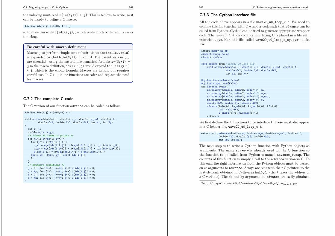
C.7 Migrating loops to C via Cython 567
the indexing must read u[i*(Ny+1) + j]. This is tedious to write, so itcan be handy to define a C macro,
#define idx(i,j) (i)*(Ny+1) + j
so that we can write u[idx(i,j)], which reads much better and is easierto debug.
Be careful with macro definitionsMacros just perform simple text substitutions: idx(hello,world)is expanded to (hello)*(Ny+1) + world. The parenthesis in (i)are essential - using the natural mathematical formula i*(Ny+1) +j in the macro definition, idx(i-1,j) would expand to i-1*(Ny+1)+ j, which is the wrong formula. Macros are handy, but requirescareful use. In C++, inline functions are safer and replace the needfor macros.
C.7.2 The complete C code
The C version of our function advance can be coded as follows.
#define idx(i,j) (i)*(Ny+1) + j
void advance(double* u, double* u_n, double* u_nm1, double* f,double Cx2, double Cy2, double dt2, int Nx, int Ny)
int i, j;double u_xx, u_yy;/* Scheme at interior points */for (i=1; i<=Nx-1; i++)
for (j=1; j<=Ny-1; j++) u_xx = u_n[idx(i-1,j)] - 2*u_n[idx(i,j)] + u_n[idx(i+1,j)];u_yy = u_n[idx(i,j-1)] - 2*u_n[idx(i,j)] + u_n[idx(i,j+1)];u[idx(i,j)] = 2*u_n[idx(i,j)] - u_nm1[idx(i,j)] +
Cx2*u_xx + Cy2*u_yy + dt2*f[idx(i,j)];
/* Boundary conditions */j = 0; for (i=0; i<=Nx; i++) u[idx(i,j)] = 0;j = Ny; for (i=0; i<=Nx; i++) u[idx(i,j)] = 0;i = 0; for (j=0; j<=Ny; j++) u[idx(i,j)] = 0;i = Nx; for (j=0; j<=Ny; j++) u[idx(i,j)] = 0;
568 C Software engineering; wave equation model
C.7.3 The Cython interface file
All the code above appears in a file wave2D_u0_loop_c.c. We need tocompile this file together with C wrapper code such that advance can becalled from Python. Cython can be used to generate appropriate wrappercode. The relevant Cython code for interfacing C is placed in a file withextension .pyx. Here this file, called wave2D_u0_loop_c_cy.pyx1, lookslike
import numpy as npcimport numpy as npcimport cython
cdef extern from "wave2D_u0_loop_c.h":void advance(double* u, double* u_n, double* u_nm1, double* f,
double Cx2, double Cy2, double dt2,int Nx, int Ny)
@cython.boundscheck(False)@cython.wraparound(False)def advance_cwrap(
np.ndarray[double, ndim=2, mode=’c’] u,np.ndarray[double, ndim=2, mode=’c’] u_n,np.ndarray[double, ndim=2, mode=’c’] u_nm1,np.ndarray[double, ndim=2, mode=’c’] f,double Cx2, double Cy2, double dt2):advance(&u[0,0], &u_n[0,0], &u_nm1[0,0], &f[0,0],
Cx2, Cy2, dt2,u.shape[0]-1, u.shape[1]-1)
return u
We first declare the C functions to be interfaced. These must also appearin a C header file, wave2D_u0_loop_c.h,
extern void advance(double* u, double* u_n, double* u_nm1, double* f,double Cx2, double Cy2, double dt2,int Nx, int Ny);
The next step is to write a Cython function with Python objects asarguments. The name advance is already used for the C function sothe function to be called from Python is named advance_cwrap. Thecontents of this function is simply a call to the advance version in C. Tothis end, the right information from the Python objects must be passedon as arguments to advance. Arrays are sent with their C pointers to thefirst element, obtained in Cython as &u[0,0] (the & takes the address ofa C variable). The Nx and Ny arguments in advance are easily obtained
1 http://tinyurl.com/nu656p2/wave/wave2D_u0/wave2D_u0_loop_c_cy.pyx
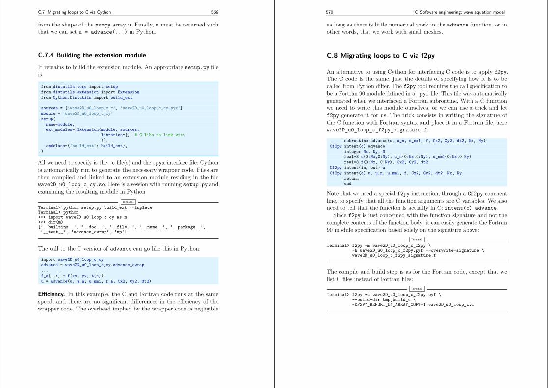
C.7 Migrating loops to C via Cython 569
from the shape of the numpy array u. Finally, u must be returned suchthat we can set u = advance(...) in Python.
C.7.4 Building the extension module
It remains to build the extension module. An appropriate setup.py fileis
from distutils.core import setupfrom distutils.extension import Extensionfrom Cython.Distutils import build_ext
sources = [’wave2D_u0_loop_c.c’, ’wave2D_u0_loop_c_cy.pyx’]module = ’wave2D_u0_loop_c_cy’setup(
name=module,ext_modules=[Extension(module, sources,
libraries=[], # C libs to link with)],
cmdclass=’build_ext’: build_ext,)
All we need to specify is the .c file(s) and the .pyx interface file. Cythonis automatically run to generate the necessary wrapper code. Files arethen compiled and linked to an extension module residing in the filewave2D_u0_loop_c_cy.so. Here is a session with running setup.py andexamining the resulting module in Python
Terminal
Terminal> python setup.py build_ext --inplaceTerminal> python>>> import wave2D_u0_loop_c_cy as m>>> dir(m)[’__builtins__’, ’__doc__’, ’__file__’, ’__name__’, ’__package__’,’__test__’, ’advance_cwrap’, ’np’]
The call to the C version of advance can go like this in Python:
import wave2D_u0_loop_c_cyadvance = wave2D_u0_loop_c_cy.advance_cwrap...f_a[:,:] = f(xv, yv, t[n])u = advance(u, u_n, u_nm1, f_a, Cx2, Cy2, dt2)
Efficiency. In this example, the C and Fortran code runs at the samespeed, and there are no significant differences in the efficiency of thewrapper code. The overhead implied by the wrapper code is negligible
570 C Software engineering; wave equation model
as long as there is little numerical work in the advance function, or inother words, that we work with small meshes.
C.8 Migrating loops to C via f2py
An alternative to using Cython for interfacing C code is to apply f2py.The C code is the same, just the details of specifying how it is to becalled from Python differ. The f2py tool requires the call specification tobe a Fortran 90 module defined in a .pyf file. This file was automaticallygenerated when we interfaced a Fortran subroutine. With a C functionwe need to write this module ourselves, or we can use a trick and letf2py generate it for us. The trick consists in writing the signature ofthe C function with Fortran syntax and place it in a Fortran file, herewave2D_u0_loop_c_f2py_signature.f:
subroutine advance(u, u_n, u_nm1, f, Cx2, Cy2, dt2, Nx, Ny)Cf2py intent(c) advance
integer Nx, Ny, Nreal*8 u(0:Nx,0:Ny), u_n(0:Nx,0:Ny), u_nm1(0:Nx,0:Ny)real*8 f(0:Nx, 0:Ny), Cx2, Cy2, dt2
Cf2py intent(in, out) uCf2py intent(c) u, u_n, u_nm1, f, Cx2, Cy2, dt2, Nx, Ny
returnend
Note that we need a special f2py instruction, through a Cf2py commentline, to specify that all the function arguments are C variables. We alsoneed to tell that the function is actually in C: intent(c) advance.
Since f2py is just concerned with the function signature and not thecomplete contents of the function body, it can easily generate the Fortran90 module specification based solely on the signature above:
Terminal
Terminal> f2py -m wave2D_u0_loop_c_f2py \-h wave2D_u0_loop_c_f2py.pyf --overwrite-signature \wave2D_u0_loop_c_f2py_signature.f
The compile and build step is as for the Fortran code, except that welist C files instead of Fortran files:
Terminal
Terminal> f2py -c wave2D_u0_loop_c_f2py.pyf \--build-dir tmp_build_c \-DF2PY_REPORT_ON_ARRAY_COPY=1 wave2D_u0_loop_c.c
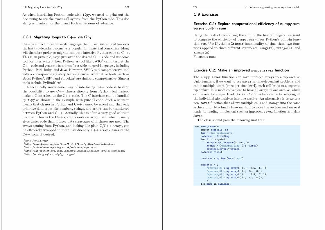
C.8 Migrating loops to C via f2py 571
As when interfacing Fortran code with f2py, we need to print out thedoc string to see the exact call syntax from the Python side. This docstring is identical for the C and Fortran versions of advance.
C.8.1 Migrating loops to C++ via f2py
C++ is a much more versatile language than C or Fortran and has overthe last two decades become very popular for numerical computing. Manywill therefore prefer to migrate compute-intensive Python code to C++.This is, in principle, easy: just write the desired C++ code and use sometool for interfacing it from Python. A tool like SWIG2 can interpret theC++ code and generate interfaces for a wide range of languages, includingPython, Perl, Ruby, and Java. However, SWIG is a comprehensive toolwith a correspondingly steep learning curve. Alternative tools, such asBoost Python3, SIP4, and Shiboken5 are similarly comprehensive. Simplertools include PyBindGen6.
A technically much easier way of interfacing C++ code is to dropthe possibility to use C++ classes directly from Python, but insteadmake a C interface to the C++ code. The C interface can be handledby f2py as shown in the example with pure C code. Such a solutionmeans that classes in Python and C++ cannot be mixed and that onlyprimitive data types like numbers, strings, and arrays can be transferredbetween Python and C++. Actually, this is often a very good solutionbecause it forces the C++ code to work on array data, which usuallygives faster code than if fancy data structures with classes are used. Thearrays coming from Python, and looking like plain C/C++ arrays, canbe efficiently wrapped in more user-friendly C++ array classes in theC++ code, if desired.
2 http://swig.org/3 http://www.boost.org/doc/libs/1_51_0/libs/python/doc/index.html4 http://riverbankcomputing.co.uk/software/sip/intro5 http://qt-project.org/wiki/Category:LanguageBindings::PySide::Shiboken6 http://code.google.com/p/pybindgen/
572 C Software engineering; wave equation model
C.9 Exercises
Exercise C.1: Explore computational efficiency of numpy.sumversus built-in sumUsing the task of computing the sum of the first n integers, we wantto compare the efficiency of numpy.sum versus Python’s built-in func-tion sum. Use IPython’s %timeit functionality to time these two func-tions applied to three different arguments: range(n), xrange(n), andarange(n).Filename: sumn.
Exercise C.2: Make an improved numpy.savez functionThe numpy.savez function can save multiple arrays to a zip archive.Unfortunately, if we want to use savez in time-dependent problems andcall it multiple times (once per time level), each call leads to a separatezip archive. It is more convenient to have all arrays in one archive, whichcan be read by numpy.load. Section C.2 provides a recipe for merging allthe individual zip archives into one archive. An alternative is to write anew savez function that allows multiple calls and storage into the samearchive prior to a final close method to close the archive and make itready for reading. Implement such an improved savez function as a classSavez.
The class should pass the following unit test:
def test_Savez():import tempfile, ostmp = ’tmp_testarchive’database = Savez(tmp)for i in range(4):
array = np.linspace(0, 5+i, 3)kwargs = ’myarray_%02d’ % i: arraydatabase.savez(**kwargs)
database.close()
database = np.load(tmp+’.npz’)
expected = ’myarray_00’: np.array([ 0. , 2.5, 5. ]),’myarray_01’: np.array([ 0., 3., 6.])’myarray_02’: np.array([ 0. , 3.5, 7. ]),’myarray_03’: np.array([ 0., 4., 8.]),
for name in database:
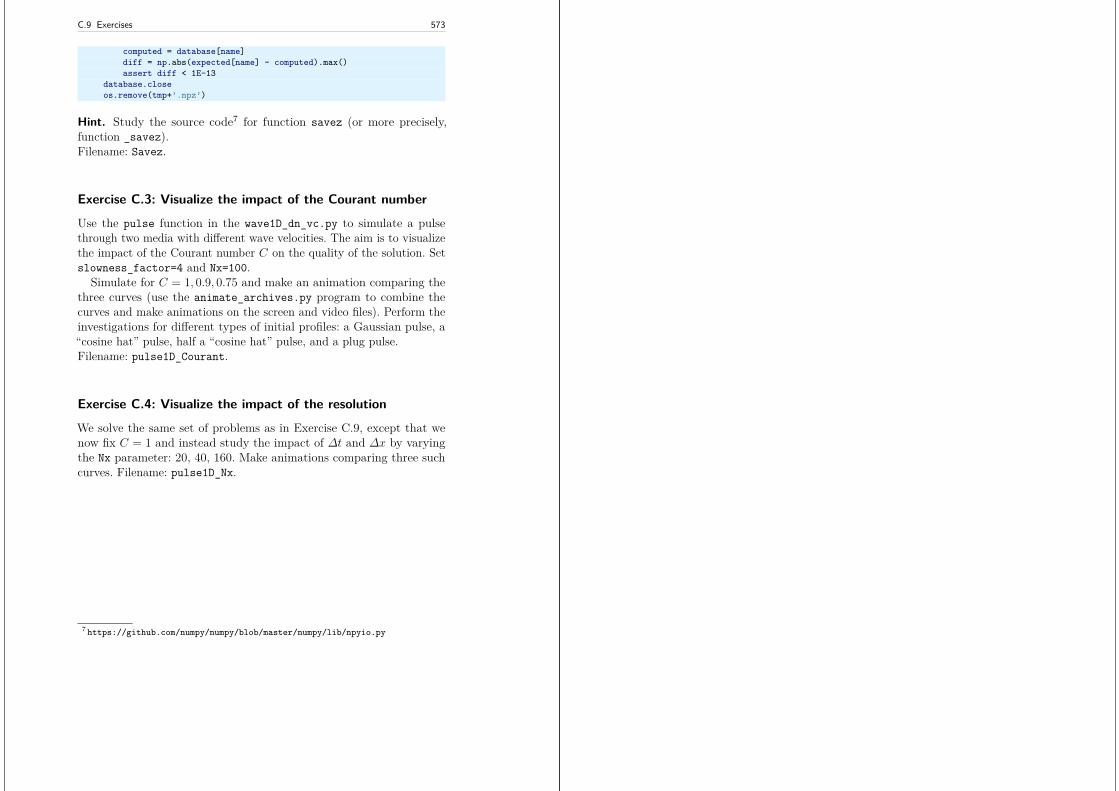
C.9 Exercises 573
computed = database[name]diff = np.abs(expected[name] - computed).max()assert diff < 1E-13
database.closeos.remove(tmp+’.npz’)
Hint. Study the source code7 for function savez (or more precisely,function _savez).Filename: Savez.
Exercise C.3: Visualize the impact of the Courant number
Use the pulse function in the wave1D_dn_vc.py to simulate a pulsethrough two media with different wave velocities. The aim is to visualizethe impact of the Courant number C on the quality of the solution. Setslowness_factor=4 and Nx=100.
Simulate for C = 1, 0.9, 0.75 and make an animation comparing thethree curves (use the animate_archives.py program to combine thecurves and make animations on the screen and video files). Perform theinvestigations for different types of initial profiles: a Gaussian pulse, a“cosine hat” pulse, half a “cosine hat” pulse, and a plug pulse.Filename: pulse1D_Courant.
Exercise C.4: Visualize the impact of the resolution
We solve the same set of problems as in Exercise C.9, except that wenow fix C = 1 and instead study the impact of ∆t and ∆x by varyingthe Nx parameter: 20, 40, 160. Make animations comparing three suchcurves. Filename: pulse1D_Nx.
7 https://github.com/numpy/numpy/blob/master/numpy/lib/npyio.py
References
[1] O. Axelsson. Iterative Solution Methods. Cambridge UniversityPress, 1996.
[2] R. Barrett, M. Berry, T. F. Chan, J. Demmel, J. Donato, J. Dongarra,V. Eijkhout, R. Pozo, C. Romine, and H. Van der Vorst. Templatesfor the Solution of Linear Systems: Building Blocks for IterativeMethods. SIAM, second edition, 1994. http://www.netlib.org/linalg/html_templates/Templates.html.
[3] D. Duran. Numerical Methods for Fluid Dynamics - With Applica-tions to Geophysics. Springer, second edition, 2010.
[4] C. A. J. Fletcher. Computational Techniques for Fluid Dynamics,Vol. 1: Fundamental and General Techniques. Springer, secondedition, 2013.
[5] C. Greif and U. M. Ascher. A First Course in Numerical Methods.Computational Science and Engineering. SIAM, 2011.
[6] E. Hairer, S. P. Nørsett, and G. Wanner. Solving Ordinary Differen-tial Equations I. Nonstiff Problems. Springer, 1993.
[7] M. Hjorth-Jensen. Computational Physics. Institute ofPhysics Publishing, 2016. https://github.com/CompPhysics/ComputationalPhysics1/raw/gh-pages/doc/Lectures/lectures2015.pdf.
[8] C. T. Kelley. Iterative Methods for Linear and Nonlinear Equations.SIAM, 1995.
[9] H. P. Langtangen. Finite Difference Computing with ExponentialDecay Models. Lecture Notes in Computational Science and Engi-neering. Springer, 2016. http://hplgit.github.io/decay-book/
© 2016, Hans Petter Langtangen, Svein Linge. Released under CC Attribution 4.0 license
576 REFERENCES
doc/web/.[10] H. P. Langtangen. A Primer on Scientific Programming with Python.
Texts in Computational Science and Engineering. Springer, fifthedition, 2016.
[11] H. P. Langtangen and G. K. Pedersen. Scaling of DifferentialEquations. Simula Springer Brief Series. Springer, 2016. http://hplgit.github.io/scaling-book/doc/web/.
[12] L. Lapidus and G. F. Pinder. Numerical Solution of Partial Differ-ential Equations in Science and Engineering. Wiley, 1982.
[13] R. LeVeque. Finite Difference Methods for Ordinary and PartialDifferential Equations: Steady-State and Time-Dependent Problems.SIAM, 2007.
[14] I. P. Omelyan, I. M. Mryglod, and R. Folk. Optimized forest-ruth-and suzuki-like algorithms for integration of motion in many-bodysystems. Computer Physics Communication, 146(2):188–202, 2002.
[15] R. Rannacher. Finite element solution of diffusion problems withirregular data. Numerische Mathematik, 43:309–327, 1984.
[16] Y. Saad. Iterative Methods for Sparse Linear Systems. SIAM,second edition, 2003. http://www-users.cs.umn.edu/~saad/IterMethBook_2ndEd.pdf.
[17] J. Strikwerda. Numerical Solution of Partial Differential Equationsin Science and Engineering. SIAM, second edition, 2007.
[18] L. N. Trefethen. Trefethen’s index cards - Forty years of notes aboutPeople, Words and Mathematics. World Scientific, 2011.
Index
3D visualization, 210
alternating mesh, 53amplification factor, 279animation, 14argparse (Python module), 73ArgumentParser (Python class),
73arithmetic mean, 163array computing, 137array slices, 137averaging
arithmetic, 163geometric, 68, 163harmonic, 163
boundary conditionopen (radiation), 177
boundary conditionsDirichlet, 150Neumann, 150periodic, 179
C extension module, 559
C/Python array storage, 564callback function, 125centered difference, 3central difference approximation,
249Cholesky factorization, 336closure, 132column-major ordering, 564conjugate gradient method, 338continuation method, 461, 485correction terms, 509Courant number, 190Cython, 555cython -a (Python-C translation
in HTML), 558
decay ODE, 502declaration of variables in Cython,
557diffusion coefficient, 247
piecewise constant, 295non-constant, 293
diffusion equation1D, 247
577
578 INDEX
2D, 3032D, banded matrix, 3082D, implementation, 3112D, implementation (sparse),
3172D, numbering of mesh points,
3042D, sparse matrix, 3072D, verification (conv. rates),
3162D, verification (exact num.
sol.), 3151D, boundary condition, 2481D, Crank-Nicolson scheme,
2681D, discrete equations, 2491D, explicit scheme, 2481D, Forward Euler scheme, 2491D, Fourier number, 2491D, Implementation, 2941D, implementation (FE), 2511D, implicit schemes, 2631D, initial boundary value
problem, 2481D, initial condition, 2481D, mesh Fourier number, 2491D, numerical experiments,
2571D, theta rule, 2701D, tridiagonal matrix, 2671D, verification (BE), 2671D, verification (CN), 2701D, verification (FE), 253implementation, 296axi-symmetric diffusion, 299diffusion coefficient, 247source term, 249spherically-symmetric diffu-
sion, 302stationary solution, 247, 295
diffusion limit of random walk, 348dimensionless number, 249Dirichlet conditions, 150discrete Fourier transform, 187distutils, 559DOF (degree of freedom), 81domain, 249
energy estimates (diffusion), 377energy principle, 41error
global, 28Euler-Cromer scheme, 46explicit discretization methods, 249
finite differencesbackward, 496centered, 3, 498forward, 497
fixed-point iteration, 425Flash (video format), 14Fokker-Planck equation, 362forced vibrations, 67Fortran array storage, 564Fortran subroutine, 561forward difference approximation,
249forward-backward Euler-Cromer
scheme, 46Fourier series, 187Fourier transform, 187fractional step methods, 462frequency (of oscillations), 2
Gauss-Seidel method, 329geometric mean, 68, 163Gnuplot, 210
harmonic average, 163heat equation, 247
INDEX 579
homogeneous Dirichlet conditions,150
homogeneous Neumann conditions,150
HTML5 video tag, 15Hz (unit), 2
index set notation, 153, 205interrupt a program by Ctrl+c, 360
Jacobi method, 322
lambda function (Python), 141Laplace equation, 247linearization, 424
explicit time integration, 422fixed-point iteration, 425Picard iteration, 425successive substitutions, 425
LU factorization, 336
making movies, 14Mayavi, 212mechanical energy, 41mechanical vibrations, 2mesh
finite differences, 2, 112mesh function, 2, 113, 249mesh points, 249MP4 (video format), 14
Neumann conditions, 150nonlinear restoring force, 67nonlinear spring, 67nose, 7, 127
Ogg (video format), 14open boundary condition, 177operator splitting, 462oscillations, 2
parallelism, 137
period (of oscillations), 2periodic boundary conditions, 179phase plane plot, 37Picard iteration, 425plotslopes.py, 10Plotter class (SciTools), 360preconditioning, 339, 380pytest, 7, 127
radiation condition, 177random walk, 342red-black numbering, 332relaxation, 323relaxation (nonlinear equations),
430resonance, 104Richardson iteration, 380row-major ordering, 564
scalar code, 137scitools movie command, 16scitools.avplotter, 360seed (random numbers), 346setup.py, 559single Picard iteration technique,
426slice, 137slope marker (in convergence plots),
10SOR method, 330splitting ODEs, 462stability criterion, 29, 190staggered Euler-Cromer scheme, 53staggered mesh, 53stationary solution, 247stencil
1D wave equation, 113Neumann boundary, 151
stochastic difference equation, 361stochastic ODE, 362Stoermer-Verlet algorithm, 51
580 INDEX
stopping criteria (nonlinear prob-lems), 426, 442
Strang splitting, 463successive substitutions, 425symplectic scheme, 47
test function, 7, 127truncation error
Backward Euler scheme, 496correction terms, 509Crank-Nicolson scheme, 498Forward Euler scheme, 497general, 493table of formulas, 499
unit testing, 7, 127upwind difference, 394
vectorization, 6, 137, 345verification, 346, 514
convergence rates, 8hand calculations, 7polynomial solution, 127polynomial solutions, 8
vibration ODE, 2video formats, 14visualization of 2D scalar fields, 210
wave equation1D, 1111D, analytical properties, 1851D, exact numerical solution,
1891D, finite difference method,
1121D, implementation, 1251D, stability, 1902D, implementation, 203
waveson a string, 111
WebM (video format), 14
Wiener process, 362wrapper code, 561