Embed Size (px)
Citation preview
Finite-Difference Schemes for the Black-Scholes Equation with Non-smooth Payoff Initial Conditions
Issues with the Greeks in simple schemes
Introduction[This lecture will be supplemented with C++ code in a lab session provided separately.]
In previous lectures I gave some examples which show how various commonly used finite-difference schemes behave with simple smooth "payoffs". With smooth payoffs the Douglas finite-difference scheme gives much better results than Crank-Nicolson. In this session we will look at how these methods behave when applied to real-world option-pricing problems. This will highlight the potentially nasty behaviour of both Crank-Nicolson and Douglas finite-difference schemes when applied to simple option-pricing prob-lems. The discontinuous nature of the payoff or its derivative in the neighbourhood of the strike induces slowly decaying oscillations into the solution of the finite-difference equations, when we use a larger time-step (which is the main point of introducing FD schemes in the first place.) These introduce small errors into the valuation itself, and undermine attempts to compute d, G and other "derivative" quantities in the neighbourhood of the strike. Note that, even with the oscillatory components small in the valuation error, the effect on the slope of the function is larger (generating larger errors in d), and there are even larger errors in G.
In this session I also look at the three-time-level version of the Douglas scheme. This chapter shows how the problem of larger errors in the Greeks can be cured, in that the oscillations can be removed, at least for our test payoffs, and the method ("three-time-level Douglas") will be used initially as the basis of our programme to define benchmark numerical algorithms. Later we shall look at some recent work by Evans and Chawla, and Giles and Carter.
The problems with the Crank-Nicolson scheme, and its resolution, are exemplified by a test problem with a = 8. Although the error in the valuation is small, we get an error in G near the strike of 12% of its exact value, and an error in q of 200%. In the corresponding three-time-level Douglas solution, the error in G near the strike is reduced to 0.2%, and that in q to 2.6%.
279

[This lecture will be supplemented with C++ code in a lab session provided separately.]
In previous lectures I gave some examples which show how various commonly used finite-difference schemes behave with simple smooth "payoffs". With smooth payoffs the Douglas finite-difference scheme gives much better results than Crank-Nicolson. In this session we will look at how these methods behave when applied to real-world option-pricing problems. This will highlight the potentially nasty behaviour of both Crank-Nicolson and Douglas finite-difference schemes when applied to simple option-pricing prob-lems. The discontinuous nature of the payoff or its derivative in the neighbourhood of the strike induces slowly decaying oscillations into the solution of the finite-difference equations, when we use a larger time-step (which is the main point of introducing FD schemes in the first place.) These introduce small errors into the valuation itself, and undermine attempts to compute d, G and other "derivative" quantities in the neighbourhood of the strike. Note that, even with the oscillatory components small in the valuation error, the effect on the slope of the function is larger (generating larger errors in d), and there are even larger errors in G.
In this session I also look at the three-time-level version of the Douglas scheme. This chapter shows how the problem of larger errors in the Greeks can be cured, in that the oscillations can be removed, at least for our test payoffs, and the method ("three-time-level Douglas") will be used initially as the basis of our programme to define benchmark numerical algorithms. Later we shall look at some recent work by Evans and Chawla, and Giles and Carter.
The problems with the Crank-Nicolson scheme, and its resolution, are exemplified by a test problem with a = 8. Although the error in the valuation is small, we get an error in G near the strike of 12% of its exact value, and an error in q of 200%. In the corresponding three-time-level Douglas solution, the error in G near the strike is reduced to 0.2%, and that in q to 2.6%.
280 15. Finite-Differences and Black-Scholes
280
Finite-Difference Schemes with Three Time-LevelsVarious schemes have been proposed for treating problems introduced by considering discontinuous or non-smooth boundary/initial conditions. These schemes aim to damp fast oscillations more effectively, by adjusting the spectrum of eigenvalues of the difference matrix. Richtmyer and Morton (1957) give a list of 14 difference schemes for the diffusion equation, and recommend schemes (their numbering) 9, 11 and 13 for non-smooth initial data. Schemes 9 and 13 are also recommended for these purposes by Smith (1985). These two schemes may be regarded as the three-time-level versions of the Crank-Nicolson scheme and the Douglas scheme, since they have truncation errors of a similar character to their two-time-level counter-parts. We already know that the truncation error characteristics of the Douglas scheme make it preferable, so we shall use this. As in previous lectures, we let m denote the time-step, and n denote the x-step. The three time-level Douglas scheme is then given by
(1)
1
8- a Iun-1
m+1 + un+1m+1M +
5
4+ 2 a unm+1
=1
6Iun-1m + un+1
m + 10 unmM -1
24Iun-1m-1 + un+1
m-1 + 10 unm-1M
This type of process requires a kick-off procedure, since initially we only know u1. We use the ordinary Douglas two-time-level scheme:
(2)H1 - 6 aL Iun-1m+1 + un+1
m+1M + H10 + 12 aL unm+1 = H1 + 6 aL Iun-1m + un+1
m M + H10 - 12 aL unm
once with a Ø a ê4 , then the three-time-level scheme once with a ê4 and then again with a ê2.
This gives us our vector pair of vectors to allow the three-time-level iteration to proceed normally there-after.
Some Required Functions from previous lecturesI am going to define many functions with similar sounding names so I will ask Mathematica to not give spelling warnings (only do this if you have sure there are no mistakes in function names!)
Off@General::spell1D
15. Finite-Differences and Black-Scholes 281
281
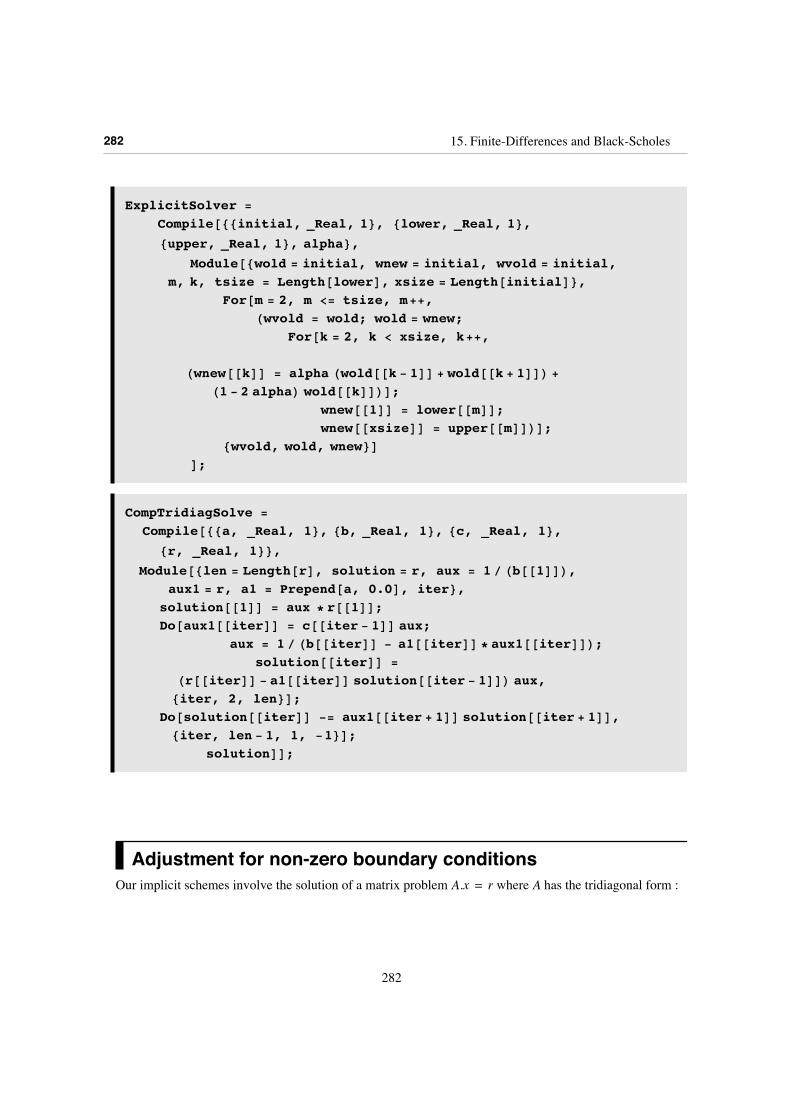
ExplicitSolver =
Compile@88initial, _Real, 1<, 8lower, _Real, 1<,
8upper, _Real, 1<, alpha<,Module@8wold = initial, wnew = initial, wvold = initial,
m, k, tsize = Length@lowerD, xsize = Length@initialD<,For@m = 2, m <= tsize, m++,
Hwvold = wold; wold = wnew;For@k = 2, k < xsize, k++,
Hwnew@@kDD = alpha Hwold@@k - 1DD + wold@@k + 1DDL +
H1 - 2 alphaL wold@@kDDLD;wnew@@1DD = lower@@mDD;wnew@@xsizeDD = upper@@mDDLD;
8wvold, wold, wnew<DD;
CompTridiagSolve =
Compile@88a, _Real, 1<, 8b, _Real, 1<, 8c, _Real, 1<,
8r, _Real, 1<<,Module@8len = Length@rD, solution = r, aux = 1 ê Hb@@1DDL,
aux1 = r, a1 = Prepend@a, 0.0D, iter<,solution@@1DD = aux * r@@1DD;Do@aux1@@iterDD = c@@iter - 1DD aux;
aux = 1 ê Hb@@iterDD - a1@@iterDD * aux1@@iterDDL;solution@@iterDD =
Hr@@iterDD - a1@@iterDD solution@@iter - 1DDL aux,8iter, 2, len<D;
Do@solution@@iterDD -= aux1@@iter + 1DD solution@@iter + 1DD,8iter, len - 1, 1, -1<D;
solutionDD;
Adjustment for non-zero boundary conditionsOur implicit schemes involve the solution of a matrix problem A.x = r where A has the tridiagonal form :
282 15. Finite-Differences and Black-Scholes
282
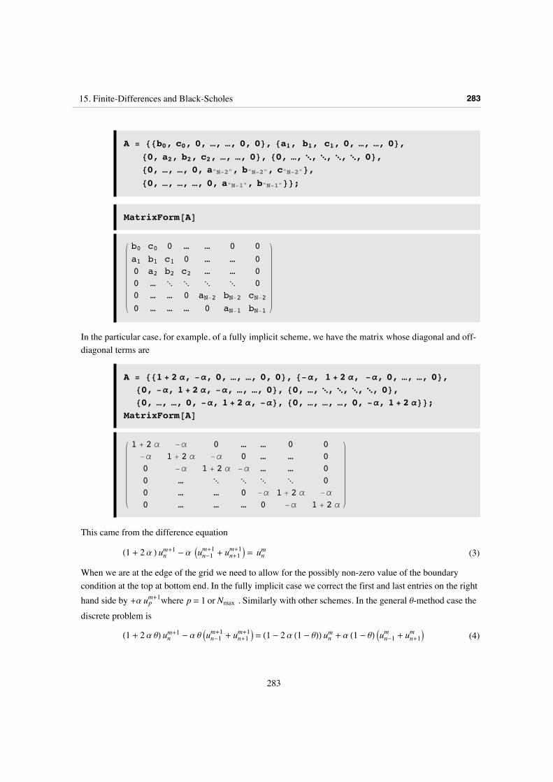
A = 88b0, c0, 0, …, …, 0, 0<, 8a1, b1, c1, 0, …, …, 0<,80, a2, b2, c2, …, …, 0<, 80, …, ¸⋱, ¸⋱, ¸⋱, ¸⋱, 0<,80, …, …, 0, a"N-2", b"N-2", c"N-2"<,80, …, …, …, 0, a"N-1", b"N-1"<<;
MatrixForm@AD
b0 c0 0 … … 0 0a1 b1 c1 0 … … 00 a2 b2 c2 … … 00 … ¸⋱ ¸⋱ ¸⋱ ¸⋱ 00 … … 0 aN-2 bN-2 cN-20 … … … 0 aN-1 bN-1
In the particular case, for example, of a fully implicit scheme, we have the matrix whose diagonal and off-diagonal terms are
A = 881 + 2 a, -a, 0, …, …, 0, 0<, 8-a, 1 + 2 a, -a, 0, …, …, 0<,80, -a, 1 + 2 a, -a, …, …, 0<, 80, …, ¸⋱, ¸⋱, ¸⋱, ¸⋱, 0<,80, …, …, 0, -a, 1 + 2 a, -a<, 80, …, …, …, 0, -a, 1 + 2 a<<;
MatrixForm@AD
1 + 2 a -a 0 … … 0 0-a 1 + 2 a -a 0 … … 00 -a 1 + 2 a -a … … 00 … ¸⋱ ¸⋱ ¸⋱ ¸⋱ 00 … … 0 -a 1 + 2 a -a0 … … … 0 -a 1 + 2 a
This came from the difference equation
(3)H1 + 2 a L unm+1 - a Iun-1m+1 + un+1
m+1M = unm
When we are at the edge of the grid we need to allow for the possibly non-zero value of the boundary condition at the top at bottom end. In the fully implicit case we correct the first and last entries on the right hand side by +a upm+1where p = 1 or Nmax . Similarly with other schemes. In the general q-method case the discrete problem is
(4)H1 + 2 a qL unm+1 - a q Iun-1m+1 + un+1
m+1M = H1 - 2 a H1 - qLL unm + a H1 - qL Iun-1m + un+1
m M
and we will add a term +a q upm+1 + aH1 - qL upm at the edges of the grid.NEEDS CARE - possible source of error. You need to think about boundary conditions. Usually such thought pays off. Sometimes a misplaced love of trees can arise from wanting to avoid thinking about boundary conditions. (But then you get bitten by exotics - see Boyle's work on barriers.)
15. Finite-Differences and Black-Scholes 283
283
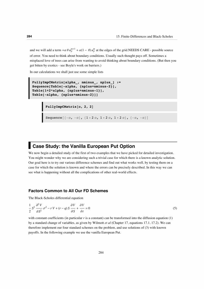
and we will add a term +a q upm+1 + aH1 - qL upm at the edges of the grid.NEEDS CARE - possible source of error. You need to think about boundary conditions. Usually such thought pays off. Sometimes a misplaced love of trees can arise from wanting to avoid thinking about boundary conditions. (But then you get bitten by exotics - see Boyle's work on barriers.)
In our calculations we shall just use some simple lists
FullyImpCMatrix[alpha_, nminus_, nplus_] :=Sequence[Table[-alpha, {nplus+nminus-2}], Table[1+2*alpha, {nplus+nminus-1}],Table[-alpha, {nplus+nminus-2}]]
FullyImpCMatrix@a, 2, 2D
Sequence@8-a, -a<, 81 + 2 a, 1 + 2 a, 1 + 2 a<, 8-a, -a<D
Case Study: the Vanilla European Put OptionWe now begin a detailed study of the first of two examples that we have picked for detailed investigation. You might wonder why we are considering such a trivial case for which there is a known analytic solution. Our goal here is to try out various difference schemes and find out what works well, by testing them on a case for which the solution is known and where the errors can be precisely described. In this way we can see what is happening without all the complications of other real-world effects.
Factors Common to All Our FD SchemesThe Black-Scholes differential equation
(5)1
2S2
¶∂2V
¶∂S2s2 - r V + Hr - qL S
¶∂V
¶∂S+¶∂V
¶∂ t= 0
with constant coefficients (in particular r is a constant) can be transformed into the diffusion equation (1) by a standard change of variables, as given by Wilmott et al (Chapter 17, equations 17.1, 17.2). We can therefore implement our four standard schemes on the problem, and use solutions of (3) with known payoffs. In the following example we use the vanilla European Put.
Standardization of Variables
284 15. Finite-Differences and Black-Scholes
284
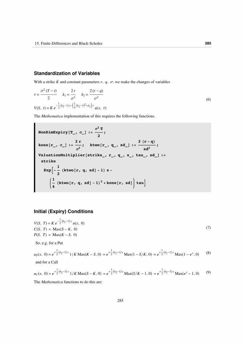
Standardization of VariablesWith a strike K and constant parameters r, q, s, we make the changes of variables
(6)t =
s2 HT - tL
2k1 =
2 r
s2k2 =
2 Hr - qL
s2
VHS, tL = K ‰-12Ik2-1M x-K
14Ik2-1M
2+k1O t uHx, tL
The Mathematica implementation of this requires the following functions.
NonDimExpiry@T_, s_D :=s2 T
2;
kone@r_, s_D :=2 r
s2; ktwo@r_, q_, sd_D :=
2 Hr - qL
sd2;
ValuationMultiplier@strike_, r_, q_, x_, tau_, sd_D :=strike
ExpB-1
2Hktwo@r, q, sdD - 1L x -
1
4Hktwo@r, q, sdD - 1L2 + kone@r, sdD tauF
Initial (Expiry) Conditions
(7)VHS, TL = K ‰
-12Ik2-1M x uHx, 0L
CHS, TL = MaxHS - K, 0LPHS, TL = MaxHK - S, 0L
So, e.g. for a Put
(8)uPHx, 0L = ‰+12Ik2-1M x 1 êK MaxHK - S, 0L = ‰
+12Ik2-1M x MaxH1 - S êK, 0L = ‰
+12Ik2-1M x MaxH1 - ‰x, 0L
and for a Call
(9)uCHx, 0L = ‰+12Ik2-1M x 1 êK MaxHS - K, 0L = ‰
+12Ik2-1M x MaxHS êK - 1, 0L = ‰
+12Ik2-1M x MaxH‰x - 1, 0L
The Mathematica functions to do this are:
15. Finite-Differences and Black-Scholes 285
285
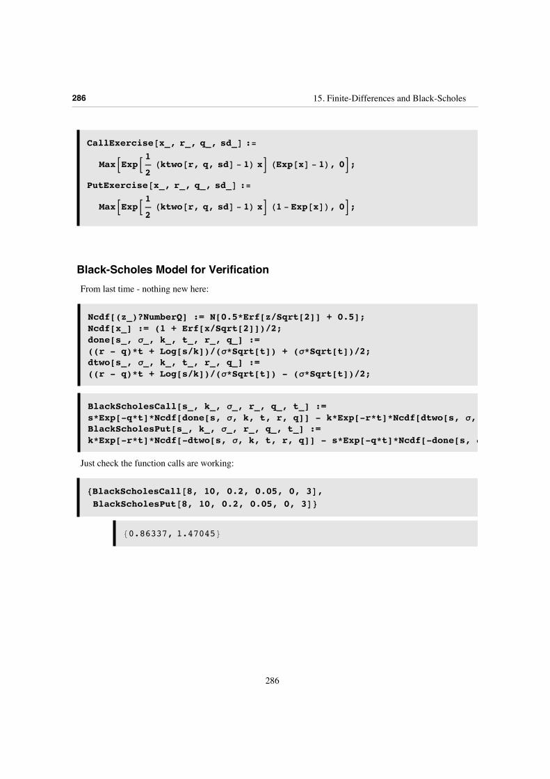
CallExercise@x_, r_, q_, sd_D :=
MaxBExpB1
2Hktwo@r, q, sdD - 1L xF HExp@xD - 1L, 0F;
PutExercise@x_, r_, q_, sd_D :=
MaxBExpB1
2Hktwo@r, q, sdD - 1L xF H1 - Exp@xDL, 0F;
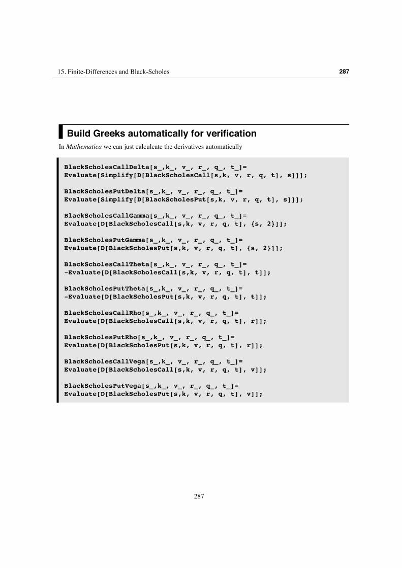
Black-Scholes Model for VerificationFrom last time - nothing new here:
Ncdf[(z_)?NumberQ] := N[0.5*Erf[z/Sqrt[2]] + 0.5]; Ncdf[x_] := (1 + Erf[x/Sqrt[2]])/2;done[s_, s_, k_, t_, r_, q_] := ((r - q)*t + Log[s/k])/(s*Sqrt[t]) + (s*Sqrt[t])/2; dtwo[s_, s_, k_, t_, r_, q_] := ((r - q)*t + Log[s/k])/(s*Sqrt[t]) - (s*Sqrt[t])/2;
BlackScholesCall[s_, k_, s_, r_, q_, t_] := s*Exp[-q*t]*Ncdf[done[s, s, k, t, r, q]] - k*Exp[-r*t]*Ncdf[dtwo[s, s, k, t, r, q]]; BlackScholesPut[s_, k_, s_, r_, q_, t_] := k*Exp[-r*t]*Ncdf[-dtwo[s, s, k, t, r, q]] - s*Exp[-q*t]*Ncdf[-done[s, s, k, t, r, q]]
Just check the function calls are working:
8BlackScholesCall@8, 10, 0.2, 0.05, 0, 3D,BlackScholesPut@8, 10, 0.2, 0.05, 0, 3D<
80.86337, 1.47045<
286 15. Finite-Differences and Black-Scholes
286
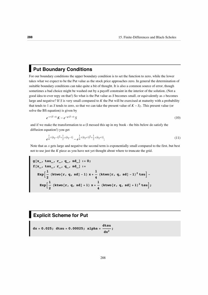
Build Greeks automatically for verificationIn Mathematica we can just calculcate the derivatives automatically
BlackScholesCallDelta[s_,k_, v_, r_, q_, t_]= Evaluate[Simplify[D[BlackScholesCall[s,k, v, r, q, t], s]]];
BlackScholesPutDelta[s_,k_, v_, r_, q_, t_]= Evaluate[Simplify[D[BlackScholesPut[s,k, v, r, q, t], s]]];
BlackScholesCallGamma[s_,k_, v_, r_, q_, t_]= Evaluate[D[BlackScholesCall[s,k, v, r, q, t], {s, 2}]];
BlackScholesPutGamma[s_,k_, v_, r_, q_, t_]= Evaluate[D[BlackScholesPut[s,k, v, r, q, t], {s, 2}]];
BlackScholesCallTheta[s_,k_, v_, r_, q_, t_]= -Evaluate[D[BlackScholesCall[s,k, v, r, q, t], t]];
BlackScholesPutTheta[s_,k_, v_, r_, q_, t_]= -Evaluate[D[BlackScholesPut[s,k, v, r, q, t], t]];
BlackScholesCallRho[s_,k_, v_, r_, q_, t_]= Evaluate[D[BlackScholesCall[s,k, v, r, q, t], r]];
BlackScholesPutRho[s_,k_, v_, r_, q_, t_]= Evaluate[D[BlackScholesPut[s,k, v, r, q, t], r]];
BlackScholesCallVega[s_,k_, v_, r_, q_, t_]= Evaluate[D[BlackScholesCall[s,k, v, r, q, t], v]];
BlackScholesPutVega[s_,k_, v_, r_, q_, t_]= Evaluate[D[BlackScholesPut[s,k, v, r, q, t], v]];
15. Finite-Differences and Black-Scholes 287
287
Put Boundary ConditionsFor our boundary conditions the upper boundary condition is to set the function to zero, while the lower takes what we expect to be the Put value as the stock price approaches zero. In general the determination of suitable boundary conditions can take quite a bit of thought. It is also a common source of error, though sometimes a bad choice might be washed out by a payoff constraint in the interior of the solution. (Not a good idea to ever repy on that!) So what is the Put value as S becomes small, or equivalently as x becomes large and negative? If S is very small compared to K the Put will be exercised at maturity with a probability that tends to 1 as S tends to zero, so that we can take the present value of K - ST . This present value (or solve the BS equation) is given by
(10)‰-r HT-tL K - ‰-q HT-tL S
and if we make the transformation to u (I messed this up in my book - the bits below do satisfy the diffusion equation!) you get
(11)‰14t Ik2-1M
2+12x Ik2-1M - ‰
14t Ik2+1M
2+12x Ik2+1M;
Note that as x gets large and negative the second term is exponentially small compared to the first, but best not to use just the K piece as you have not yet thought about where to truncate the grid.
g@x_, tau_, r_, q_, sd_D := 0;
f@x_, tau_, r_, q_, sd_D :=
ExpB1
2Hktwo@r, q, sdD - 1L x +
1
4Hktwo@r, q, sdD - 1L2 tauF -
ExpB1
2Hktwo@r, q, sdD + 1L x +
1
4Hktwo@r, q, sdD + 1L2 tauF;
Explicit Scheme for Put
dx = 0.025; dtau = 0.00025; alpha =dtau
dx2;
288 15. Finite-Differences and Black-Scholes
288
M = 400; nminus = 160; nplus = 160;
‡ Setting the Initial (Expiry) Condition and Boundary Conditions
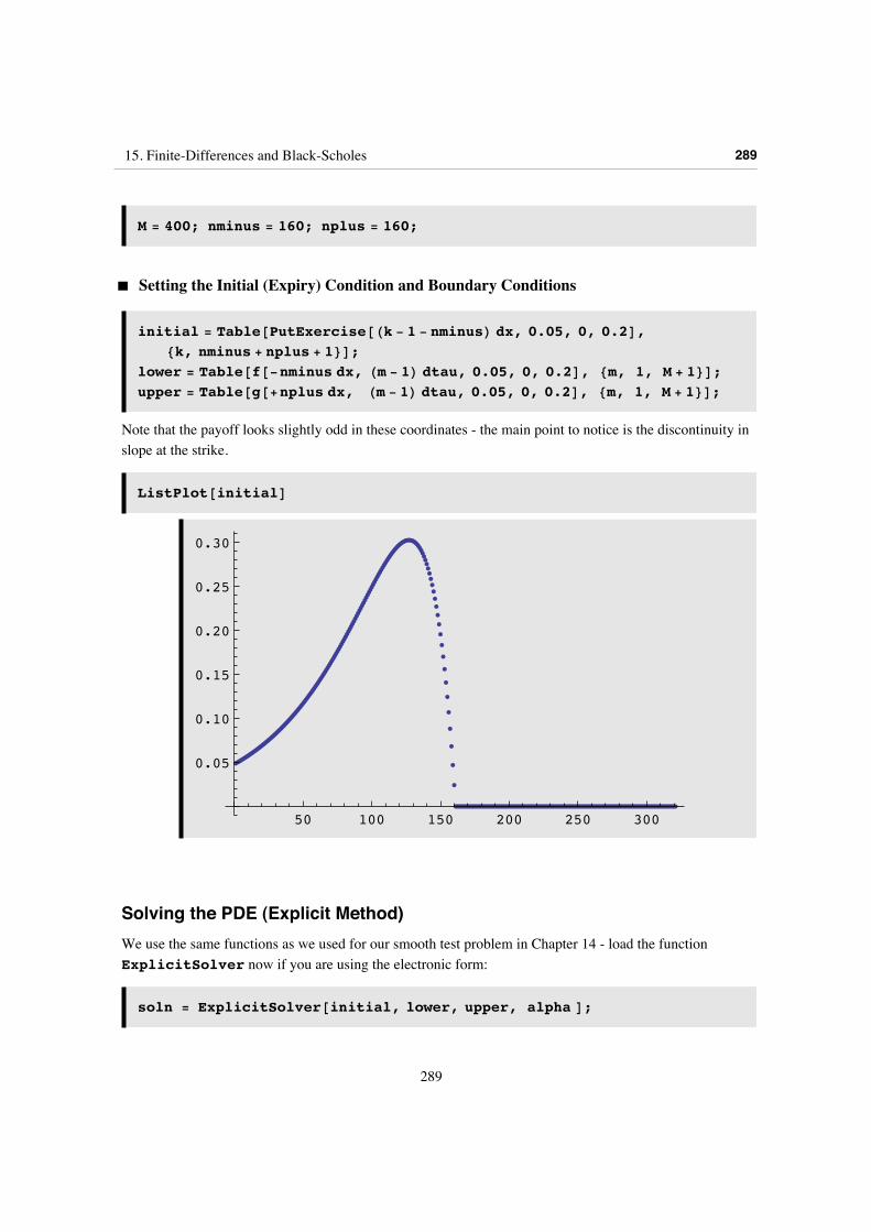
initial = Table@PutExercise@Hk - 1 - nminusL dx, 0.05, 0, 0.2D,8k, nminus + nplus + 1<D;
lower = Table@f@-nminus dx, Hm - 1L dtau, 0.05, 0, 0.2D, 8m, 1, M + 1<D;upper = Table@g@+nplus dx, Hm - 1L dtau, 0.05, 0, 0.2D, 8m, 1, M + 1<D;
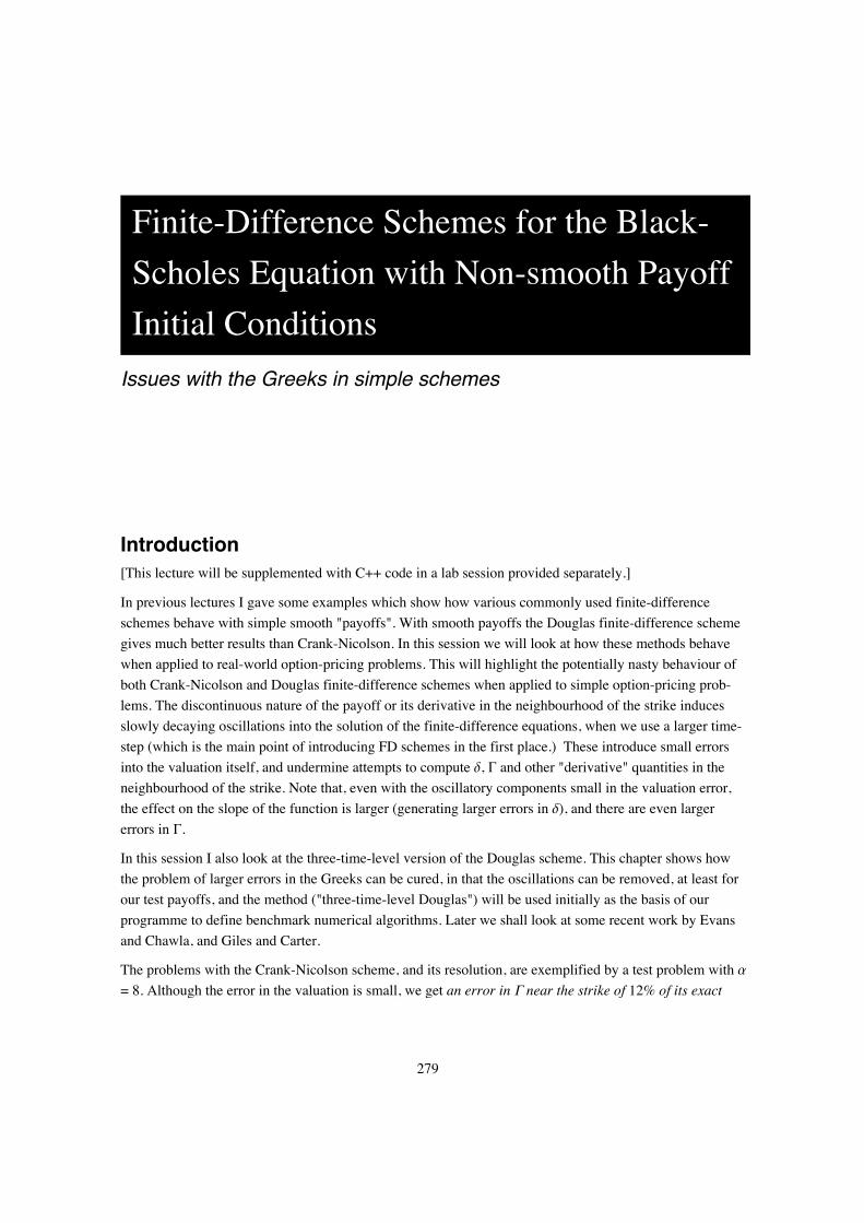
Note that the payoff looks slightly odd in these coordinates - the main point to notice is the discontinuity in slope at the strike.
ListPlot@initialD
50 100 150 200 250 300
0.05
0.10
0.15
0.20
0.25
0.30
Solving the PDE (Explicit Method)We use the same functions as we used for our smooth test problem in Chapter 14 - load the function ExplicitSolver now if you are using the electronic form:
soln = ExplicitSolver@initial, lower, upper, alpha D;
Interpolating to Supply a Continuous Function
15. Finite-Differences and Black-Scholes 289
289
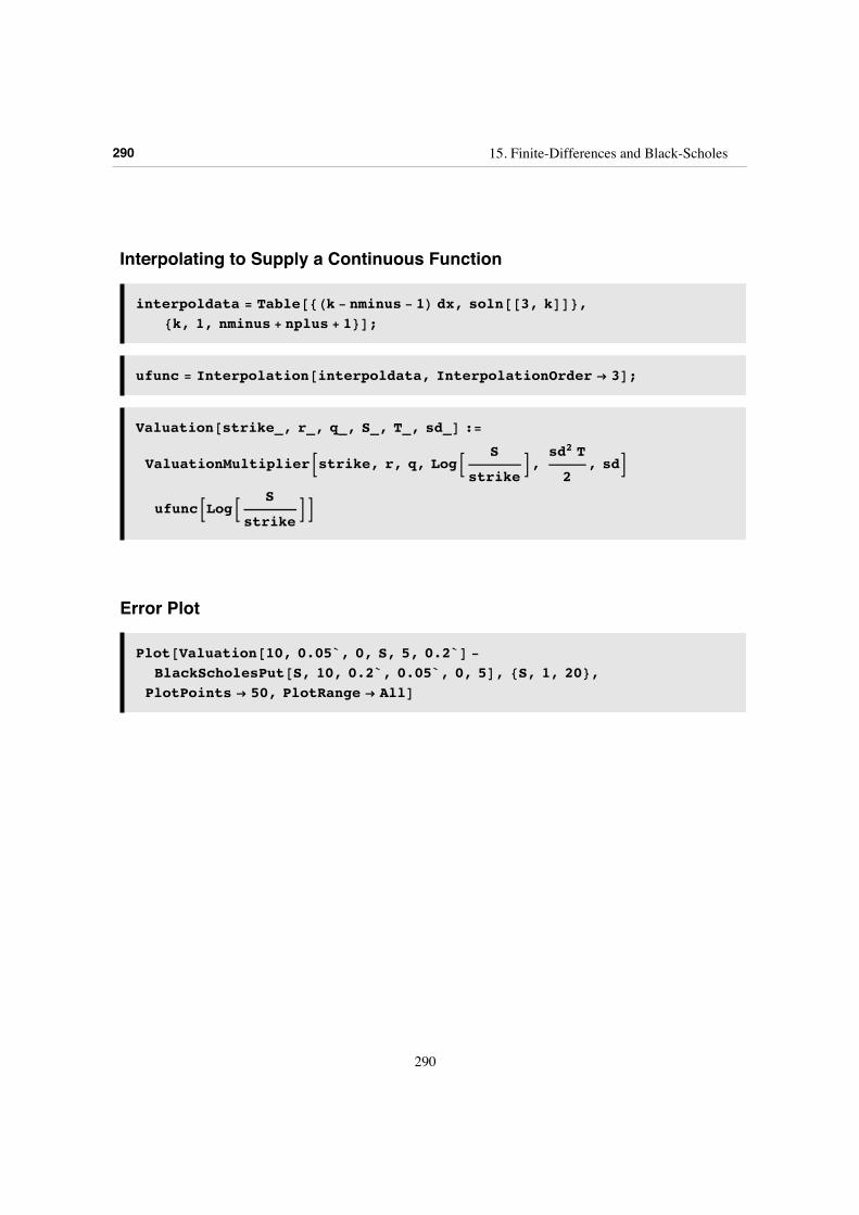
Interpolating to Supply a Continuous Function
interpoldata = Table@8Hk - nminus - 1L dx, soln@@3, kDD<,8k, 1, nminus + nplus + 1<D;
ufunc = Interpolation@interpoldata, InterpolationOrder Ø 3D;
Valuation@strike_, r_, q_, S_, T_, sd_D :=
ValuationMultiplierBstrike, r, q, LogBS
strikeF,
sd2 T
2, sdF
ufuncBLogBS
strikeFF
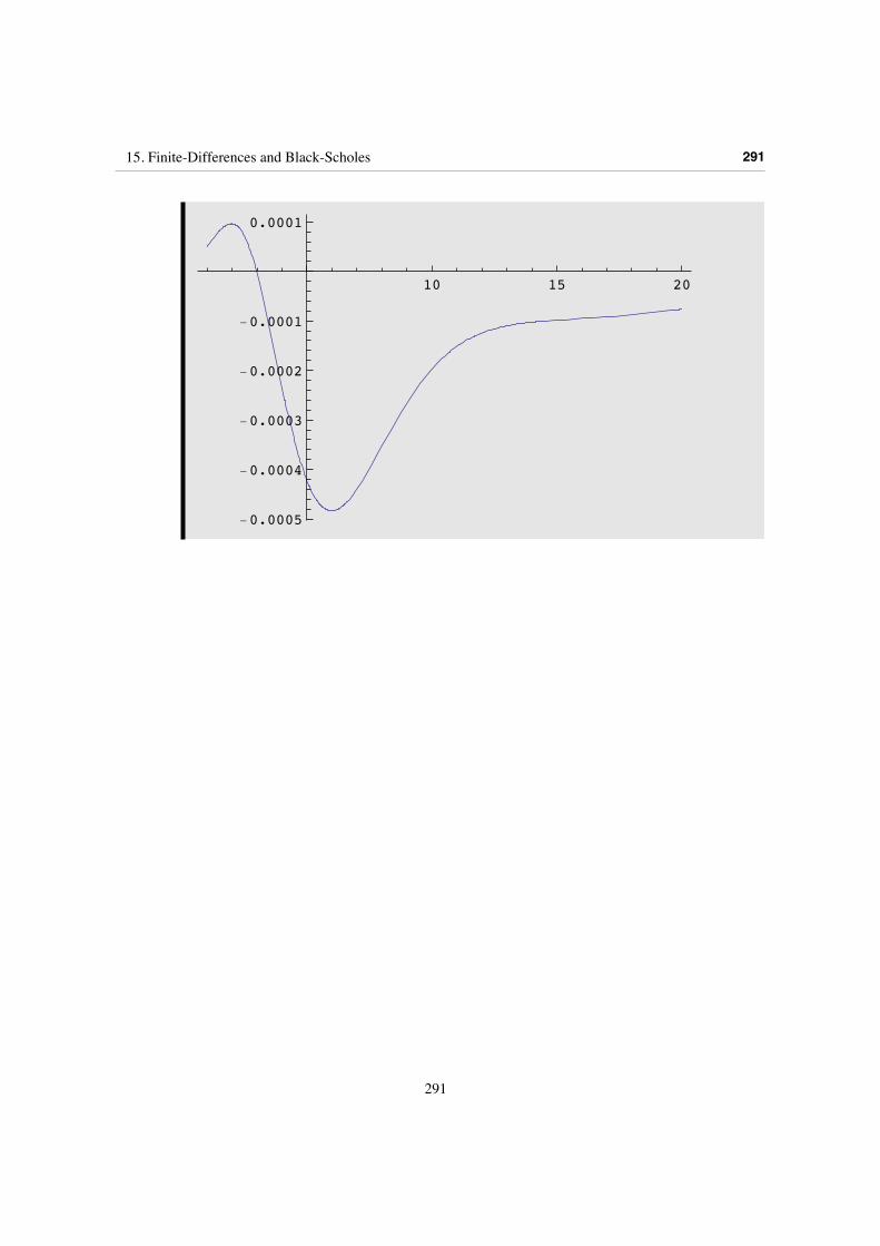
Error Plot
Plot@Valuation@10, 0.05`, 0, S, 5, 0.2`D -
BlackScholesPut@S, 10, 0.2`, 0.05`, 0, 5D, 8S, 1, 20<,PlotPoints Ø 50, PlotRange Ø AllD
290 15. Finite-Differences and Black-Scholes
290
10 15 20
-0.0005
-0.0004
-0.0003
-0.0002
-0.0001
0.0001
15. Finite-Differences and Black-Scholes 291
291

samples = TableForm@Join@88"S", "Explicit FD", "Exact", "Error"<<,Table@HPaddedForm@N@Ò1D, 85, 5<D &L êü
8S, Valuation@10, 0.05, 0, S, 5, 0.2D,BlackScholesPut@S, 10, 0.2, 0.05, 0, 5D,
Valuation@10, 0.05, 0, S, 5, 0.2D -
BlackScholesPut@S, 10, 0.2, 0.05, 0, 5D<,8S, 2, 16, 1<
DDD
S Explicit FD Exact Error2.00000 5.78870 5.78860 0.000103.00000 4.80050 4.80050 -2.16410 µ 10-6
4.00000 3.86130 3.86150 -0.000235.00000 3.02040 3.02090 -0.000426.00000 2.31040 2.31080 -0.000487.00000 1.73820 1.73870 -0.000448.00000 1.29290 1.29320 -0.000359.00000 0.95451 0.95478 -0.0002710.00000 0.70167 0.70187 -0.0002011.00000 0.51477 0.51492 -0.0001512.00000 0.37754 0.37766 -0.0001213.00000 0.27715 0.27726 -0.0001114.00000 0.20384 0.20394 -0.0001015.00000 0.15030 0.15040 -0.0001016.00000 0.11116 0.11125 -0.00010
292 15. Finite-Differences and Black-Scholes
292
Fully Implicit Scheme for PutThese algorithms are by now self-explanatory - first the initialization:
dx = 0.025; dtau = 0.00025; alpha =dtau
dx2;
M = 400; nminus = 160; nplus = 160;
initial = Table@PutExercise@Hk - 1 - nminusL dx, 0.05, 0, 0.2D,8k, nminus + nplus + 1<D;
lower = Table@f@-nminus dx, Hm - 1L dtau, 0.05, 0, 0.2D, 8m, 1, M + 1<D;upper = Table@g@+nplus dx, Hm - 1L dtau, 0.05, 0, 0.2D, 8m, 1, M + 1<D;wold = initial;wvold = wold; wnew = wold;
CMat = FullyImpCMatrix@alpha, nminus, nplusD;
Evolving the solution (this may take some time):
For[m=2, m<=M+1, m++,(wvold = wold;wold = wnew;(* Adjust the rhs for non-zero BCs *)rhs = Take[wold, {2, -2}]+Table[Which[k==1, alpha*lower[[m]],k== nplus + nminus-1, alpha*upper[[m]],True, 0],{k, 1, nplus + nminus-1}];temp = CompTridiagSolve[CMat, rhs];wnew = Join[{lower[[m]]}, temp, {upper[[m]]}])]
Interpolation and construction of valuation function:
interpoldata = Table[{(k - nminus - 1)*dx, wnew[[k]]}, {k, 1, nminus + nplus + 1}];
15. Finite-Differences and Black-Scholes 293
293
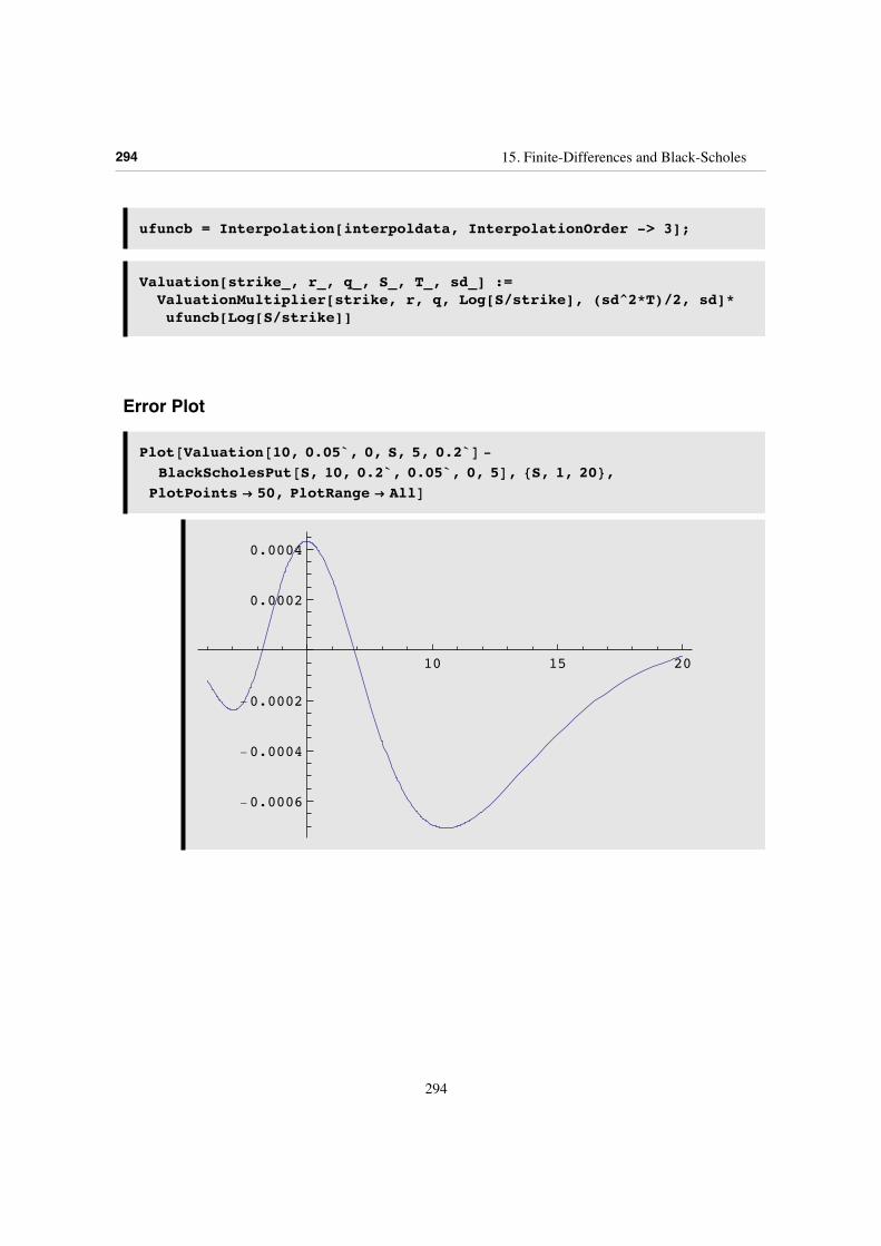
ufuncb = Interpolation[interpoldata, InterpolationOrder -> 3];
Valuation[strike_, r_, q_, S_, T_, sd_] := ValuationMultiplier[strike, r, q, Log[S/strike], (sd^2*T)/2, sd]* ufuncb[Log[S/strike]]
Error Plot
Plot@Valuation@10, 0.05`, 0, S, 5, 0.2`D -
BlackScholesPut@S, 10, 0.2`, 0.05`, 0, 5D, 8S, 1, 20<,PlotPoints Ø 50, PlotRange Ø AllD
10 15 20
-0.0006
-0.0004
-0.0002
0.0002
0.0004
294 15. Finite-Differences and Black-Scholes
294
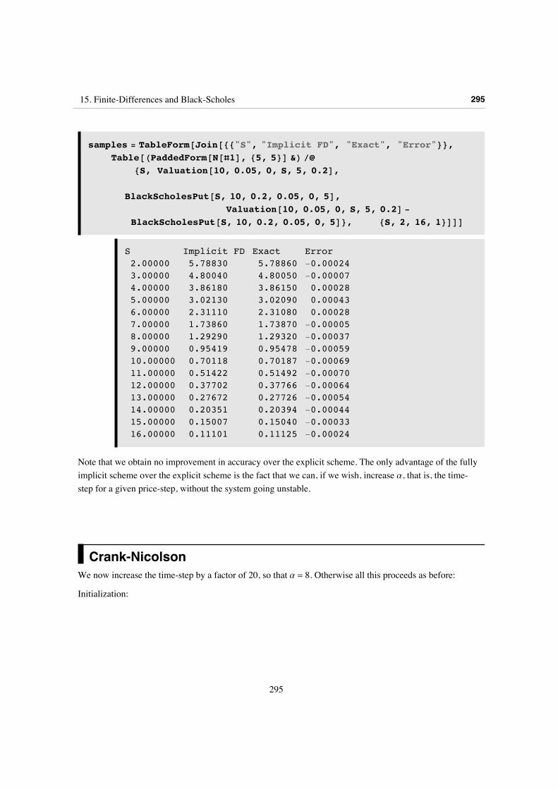
samples = TableForm@Join@88"S", "Implicit FD", "Exact", "Error"<<,Table@HPaddedForm@N@Ò1D, 85, 5<D &L êü
8S, Valuation@10, 0.05, 0, S, 5, 0.2D,
BlackScholesPut@S, 10, 0.2, 0.05, 0, 5D,Valuation@10, 0.05, 0, S, 5, 0.2D -
BlackScholesPut@S, 10, 0.2, 0.05, 0, 5D<, 8S, 2, 16, 1<DDD
S Implicit FD Exact Error2.00000 5.78830 5.78860 -0.000243.00000 4.80040 4.80050 -0.000074.00000 3.86180 3.86150 0.000285.00000 3.02130 3.02090 0.000436.00000 2.31110 2.31080 0.000287.00000 1.73860 1.73870 -0.000058.00000 1.29290 1.29320 -0.000379.00000 0.95419 0.95478 -0.0005910.00000 0.70118 0.70187 -0.0006911.00000 0.51422 0.51492 -0.0007012.00000 0.37702 0.37766 -0.0006413.00000 0.27672 0.27726 -0.0005414.00000 0.20351 0.20394 -0.0004415.00000 0.15007 0.15040 -0.0003316.00000 0.11101 0.11125 -0.00024
Note that we obtain no improvement in accuracy over the explicit scheme. The only advantage of the fully implicit scheme over the explicit scheme is the fact that we can, if we wish, increase a, that is, the time-step for a given price-step, without the system going unstable.
Crank-NicolsonWe now increase the time-step by a factor of 20, so that a = 8. Otherwise all this proceeds as before:
Initialization:
15. Finite-Differences and Black-Scholes 295
295
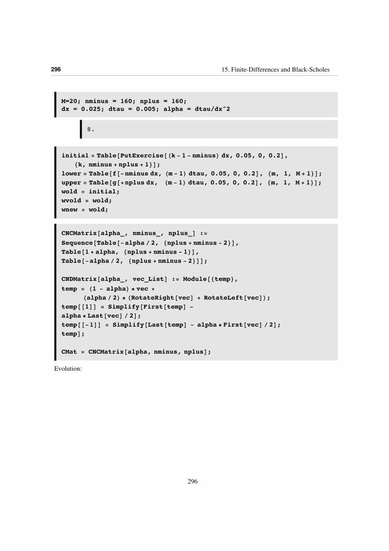
M=20; nminus = 160; nplus = 160;dx = 0.025; dtau = 0.005; alpha = dtau/dx^2
8.
initial = Table@PutExercise@Hk - 1 - nminusL dx, 0.05, 0, 0.2D,8k, nminus + nplus + 1<D;
lower = Table@f@-nminus dx, Hm - 1L dtau, 0.05, 0, 0.2D, 8m, 1, M + 1<D;upper = Table@g@+nplus dx, Hm - 1L dtau, 0.05, 0, 0.2D, 8m, 1, M + 1<D;wold = initial;wvold = wold;wnew = wold;
CNCMatrix@alpha_, nminus_, nplus_D :=Sequence@Table@-alpha ê 2, 8nplus + nminus - 2<D,Table@1 + alpha, 8nplus + nminus - 1<D,Table@-alpha ê 2, 8nplus + nminus - 2<DD;
CNDMatrix@alpha_, vec_ListD := Module@8temp<,temp = H1 - alphaL * vec +
Halpha ê 2L * HRotateRight@vecD + RotateLeft@vecDL;temp@@1DD = Simplify@First@tempD -
alpha * Last@vecD ê 2D;temp@@-1DD = Simplify@Last@tempD - alpha * First@vecD ê 2D;tempD;
CMat = CNCMatrix@alpha, nminus, nplusD;
Evolution:
296 15. Finite-Differences and Black-Scholes
296
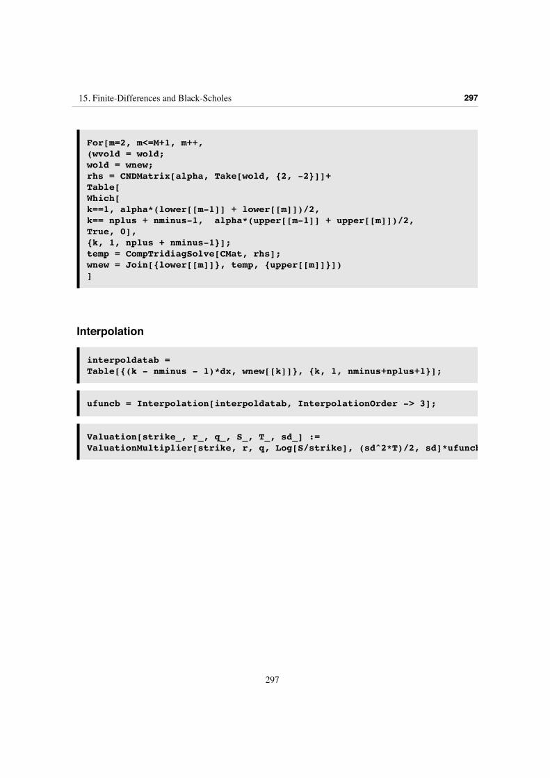
For[m=2, m<=M+1, m++,(wvold = wold;wold = wnew;rhs = CNDMatrix[alpha, Take[wold, {2, -2}]]+Table[Which[k==1, alpha*(lower[[m-1]] + lower[[m]])/2,k== nplus + nminus-1, alpha*(upper[[m-1]] + upper[[m]])/2,True, 0],{k, 1, nplus + nminus-1}];temp = CompTridiagSolve[CMat, rhs];wnew = Join[{lower[[m]]}, temp, {upper[[m]]}])]
Interpolation
interpoldatab = Table[{(k - nminus - 1)*dx, wnew[[k]]}, {k, 1, nminus+nplus+1}];
ufuncb = Interpolation[interpoldatab, InterpolationOrder -> 3];
Valuation[strike_, r_, q_, S_, T_, sd_] :=ValuationMultiplier[strike, r, q, Log[S/strike], (sd^2*T)/2, sd]*ufuncb[Log[S/strike]]
15. Finite-Differences and Black-Scholes 297
297
Error Plot
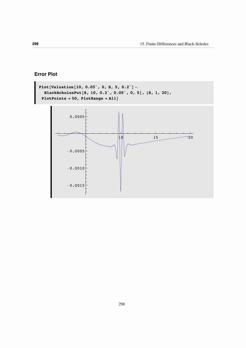
Plot@Valuation@10, 0.05`, 0, S, 5, 0.2`D -
BlackScholesPut@S, 10, 0.2`, 0.05`, 0, 5D, 8S, 1, 20<,PlotPoints Ø 50, PlotRange Ø AllD
10 15 20
-0.0015
-0.0010
-0.0005
0.0005
298 15. Finite-Differences and Black-Scholes
298
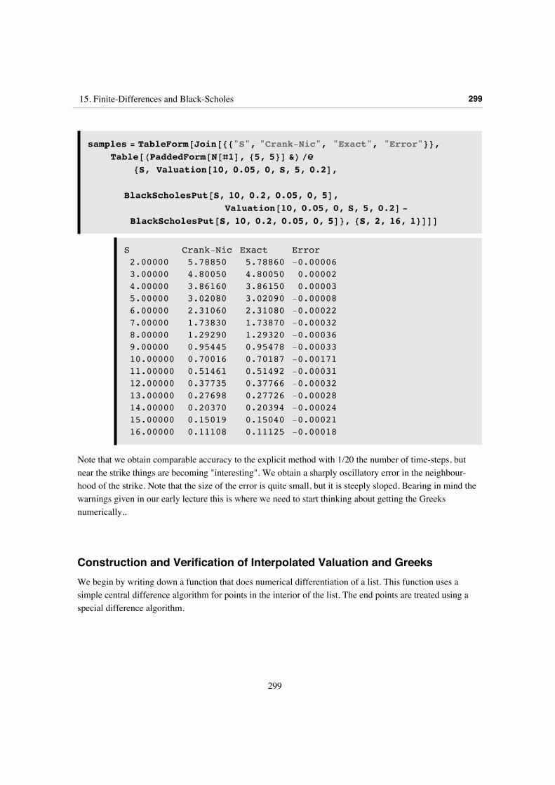
samples = TableForm@Join@88"S", "Crank-Nic", "Exact", "Error"<<,Table@HPaddedForm@N@Ò1D, 85, 5<D &L êü
8S, Valuation@10, 0.05, 0, S, 5, 0.2D,
BlackScholesPut@S, 10, 0.2, 0.05, 0, 5D,Valuation@10, 0.05, 0, S, 5, 0.2D -
BlackScholesPut@S, 10, 0.2, 0.05, 0, 5D<, 8S, 2, 16, 1<DDD
S Crank-Nic Exact Error2.00000 5.78850 5.78860 -0.000063.00000 4.80050 4.80050 0.000024.00000 3.86160 3.86150 0.000035.00000 3.02080 3.02090 -0.000086.00000 2.31060 2.31080 -0.000227.00000 1.73830 1.73870 -0.000328.00000 1.29290 1.29320 -0.000369.00000 0.95445 0.95478 -0.0003310.00000 0.70016 0.70187 -0.0017111.00000 0.51461 0.51492 -0.0003112.00000 0.37735 0.37766 -0.0003213.00000 0.27698 0.27726 -0.0002814.00000 0.20370 0.20394 -0.0002415.00000 0.15019 0.15040 -0.0002116.00000 0.11108 0.11125 -0.00018
Note that we obtain comparable accuracy to the explicit method with 1/20 the number of time-steps, but near the strike things are becoming "interesting". We obtain a sharply oscillatory error in the neighbour-hood of the strike. Note that the size of the error is quite small, but it is steeply sloped. Bearing in mind the warnings given in our early lecture this is where we need to start thinking about getting the Greeks numerically..
Construction and Verification of Interpolated Valuation and GreeksWe begin by writing down a function that does numerical differentiation of a list. This function uses a simple central difference algorithm for points in the interior of the list. The end points are treated using a special difference algorithm.
15. Finite-Differences and Black-Scholes 299
299
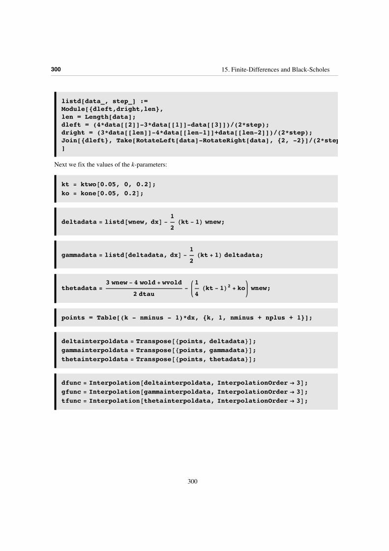
listd[data_, step_] :=Module[{dleft,dright,len},len = Length[data];dleft = (4*data[[2]]-3*data[[1]]-data[[3]])/(2*step);dright = (3*data[[len]]-4*data[[len-1]]+data[[len-2]])/(2*step);Join[{dleft}, Take[RotateLeft[data]-RotateRight[data], {2, -2}]/(2*step), {dright}]]
Next we fix the values of the k-parameters:
kt = [email protected], 0, 0.2D;ko = [email protected], 0.2D;
deltadata = listd@wnew, dxD -1
2Hkt - 1L wnew;
gammadata = listd@deltadata, dxD -1
2Hkt + 1L deltadata;
thetadata =3 wnew - 4 wold + wvold
2 dtau-
1
4Hkt - 1L2 + ko wnew;
points = Table[(k - nminus - 1)*dx, {k, 1, nminus + nplus + 1}];
deltainterpoldata = Transpose@8points, deltadata<D;gammainterpoldata = Transpose@8points, gammadata<D;thetainterpoldata = Transpose@8points, thetadata<D;
dfunc = Interpolation@deltainterpoldata, InterpolationOrder Ø 3D;gfunc = Interpolation@gammainterpoldata, InterpolationOrder Ø 3D;tfunc = Interpolation@thetainterpoldata, InterpolationOrder Ø 3D;
300 15. Finite-Differences and Black-Scholes
300
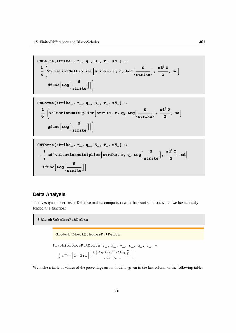
CNDelta@strike_, r_, q_, S_, T_, sd_D :=
1
SValuationMultiplierBstrike, r, q, LogB
S
strikeF,
sd2 T
2, sdF
dfuncBLogBS
strikeFF
CNGamma@strike_, r_, q_, S_, T_, sd_D :=
1
S2ValuationMultiplierBstrike, r, q, LogB
S
strikeF,
sd2 T
2, sdF
gfuncBLogBS
strikeFF
CNTheta@strike_, r_, q_, S_, T_, sd_D :=
-1
2sd2 ValuationMultiplierBstrike, r, q, LogB
S
strikeF,
sd2 T
2, sdF
tfuncBLogBS
strikeFF
Delta AnalysisTo investigate the errors in Delta we make a comparison with the exact solution, which we have already loaded as a function:
? BlackScholesPutDelta
Global`BlackScholesPutDelta
BlackScholesPutDelta@s_, k_, v_, r_, q_, t_D =
- 1
2‰-q t 1 + ErfB-
t J-2 q+2 r+v2N+2 LogBskF
2 2 t vF
We make a table of values of the percentage errors in delta, given in the last column of the following table:
15. Finite-Differences and Black-Scholes 301
301
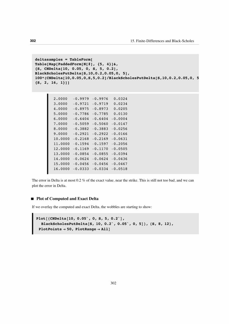
deltasamples = TableForm[Table[Map[PaddedForm[N[#], {5, 4}]&, {S, CNDelta[10, 0.05, 0, S, 5, 0.2],BlackScholesPutDelta[S,10,0.2,0.05,0, 5],100*(CNDelta[10,0.05,0,S,5,0.2]/BlackScholesPutDelta[S,10,0.2,0.05,0, 5]-1)}],{S, 2, 16, 1}]]
2.0000 -0.9979 -0.9976 0.03243.0000 -0.9721 -0.9719 0.02344.0000 -0.8975 -0.8973 0.02055.0000 -0.7786 -0.7785 0.01306.0000 -0.6404 -0.6404 -0.00047.0000 -0.5059 -0.5060 -0.01478.0000 -0.3882 -0.3883 -0.02569.0000 -0.2921 -0.2922 -0.016610.0000 -0.2168 -0.2169 -0.063111.0000 -0.1594 -0.1597 -0.205612.0000 -0.1169 -0.1170 -0.050513.0000 -0.0854 -0.0855 -0.039414.0000 -0.0624 -0.0624 -0.043615.0000 -0.0456 -0.0456 -0.046716.0000 -0.0333 -0.0334 -0.0518
The error in Delta is at most 0.2 % of the exact value, near the strike. This is still not too bad, and we can plot the error in Delta.
‡ Plot of Computed and Exact Delta
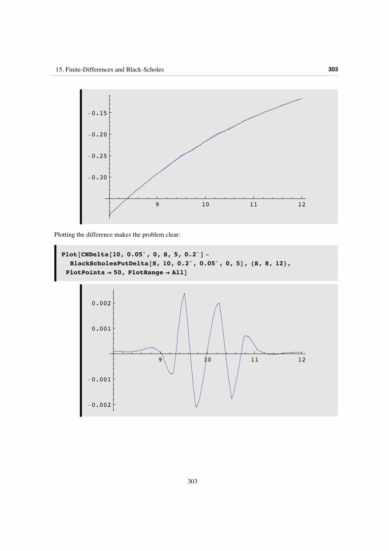
If we overlay the computed and exact Delta, the wobbles are starting to show:
Plot@8CNDelta@10, 0.05`, 0, S, 5, 0.2`D,BlackScholesPutDelta@S, 10, 0.2`, 0.05`, 0, 5D<, 8S, 8, 12<,
PlotPoints Ø 50, PlotRange Ø AllD
302 15. Finite-Differences and Black-Scholes
302
9 10 11 12
-0.30
-0.25
-0.20
-0.15
Plotting the difference makes the problem clear:
Plot@CNDelta@10, 0.05`, 0, S, 5, 0.2`D -
BlackScholesPutDelta@S, 10, 0.2`, 0.05`, 0, 5D, 8S, 8, 12<,PlotPoints Ø 50, PlotRange Ø AllD
9 10 11 12
-0.002
-0.001
0.001
0.002
15. Finite-Differences and Black-Scholes 303
303
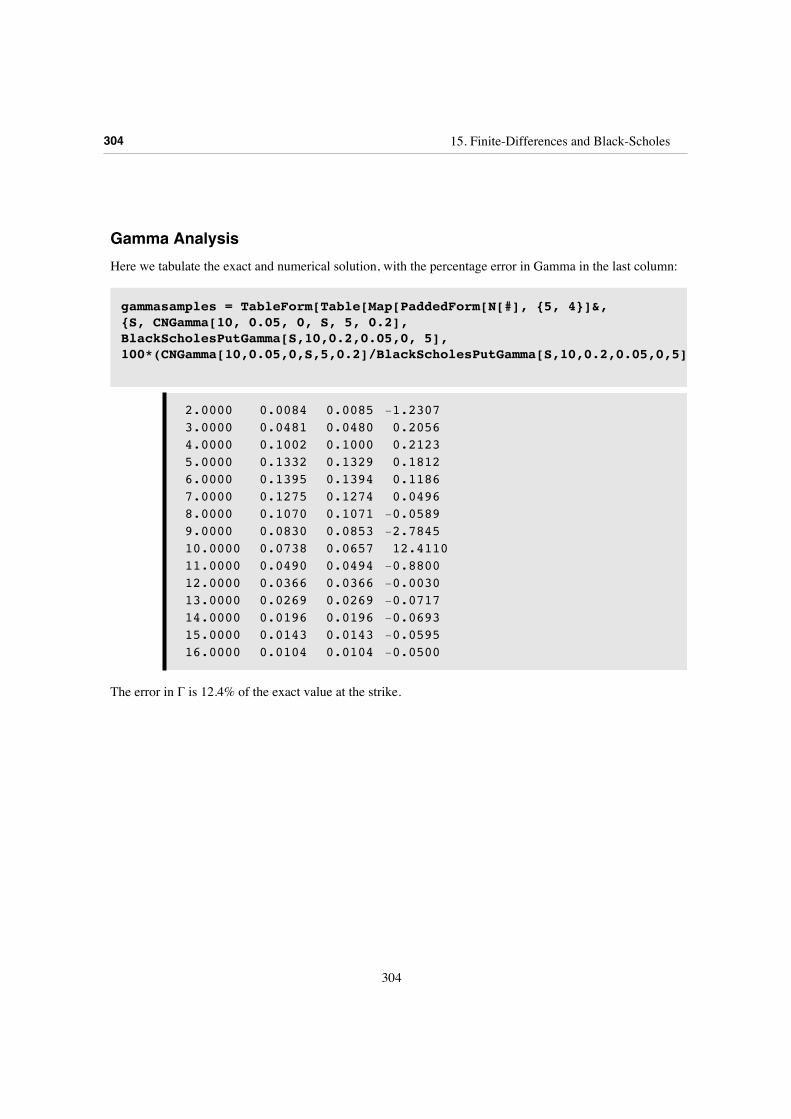
Gamma AnalysisHere we tabulate the exact and numerical solution, with the percentage error in Gamma in the last column:
gammasamples = TableForm[Table[Map[PaddedForm[N[#], {5, 4}]&, {S, CNGamma[10, 0.05, 0, S, 5, 0.2],BlackScholesPutGamma[S,10,0.2,0.05,0, 5],100*(CNGamma[10,0.05,0,S,5,0.2]/BlackScholesPutGamma[S,10,0.2,0.05,0,5]-1)}],{S, 2, 16, 1}]]
2.0000 0.0084 0.0085 -1.23073.0000 0.0481 0.0480 0.20564.0000 0.1002 0.1000 0.21235.0000 0.1332 0.1329 0.18126.0000 0.1395 0.1394 0.11867.0000 0.1275 0.1274 0.04968.0000 0.1070 0.1071 -0.05899.0000 0.0830 0.0853 -2.784510.0000 0.0738 0.0657 12.411011.0000 0.0490 0.0494 -0.880012.0000 0.0366 0.0366 -0.003013.0000 0.0269 0.0269 -0.071714.0000 0.0196 0.0196 -0.069315.0000 0.0143 0.0143 -0.059516.0000 0.0104 0.0104 -0.0500
The error in G is 12.4% of the exact value at the strike.
304 15. Finite-Differences and Black-Scholes
304
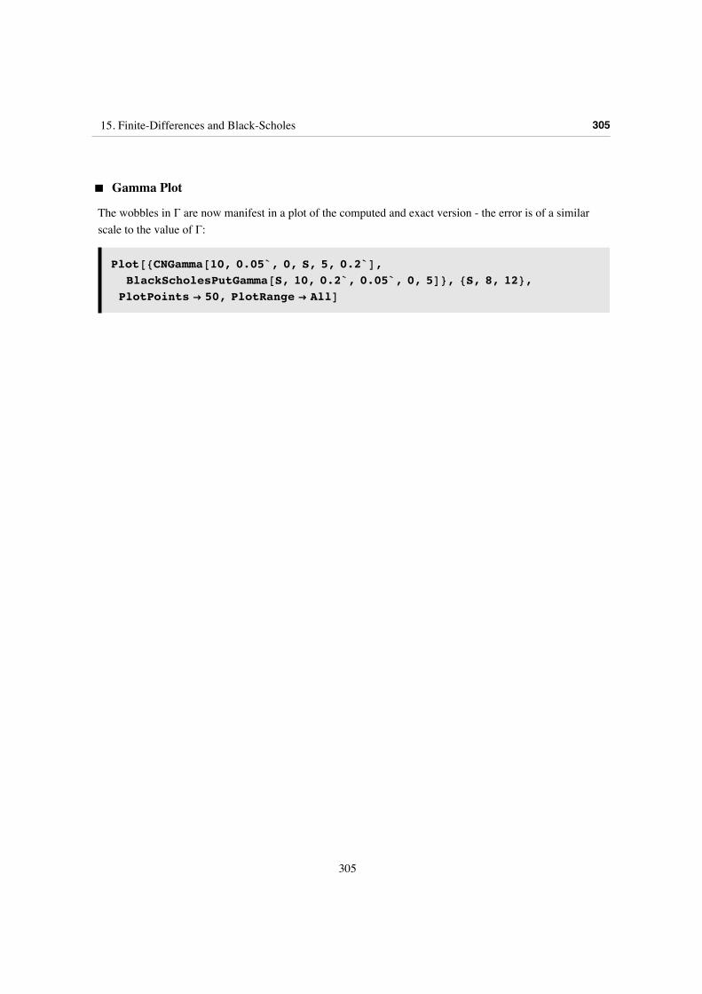
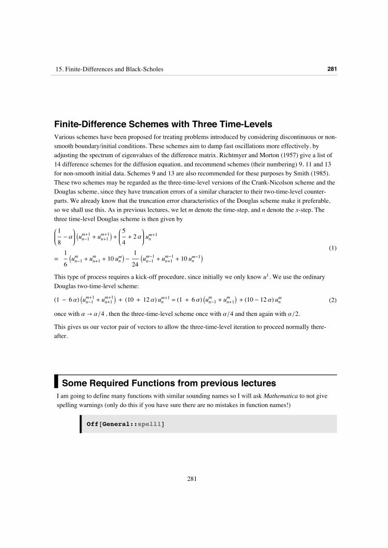
‡ Gamma Plot
The wobbles in G are now manifest in a plot of the computed and exact version - the error is of a similar scale to the value of G:
Plot@8CNGamma@10, 0.05`, 0, S, 5, 0.2`D,BlackScholesPutGamma@S, 10, 0.2`, 0.05`, 0, 5D<, 8S, 8, 12<,
PlotPoints Ø 50, PlotRange Ø AllD
15. Finite-Differences and Black-Scholes 305
305
9 10 11 12
0.05
0.06
0.07
0.08
0.09
0.10
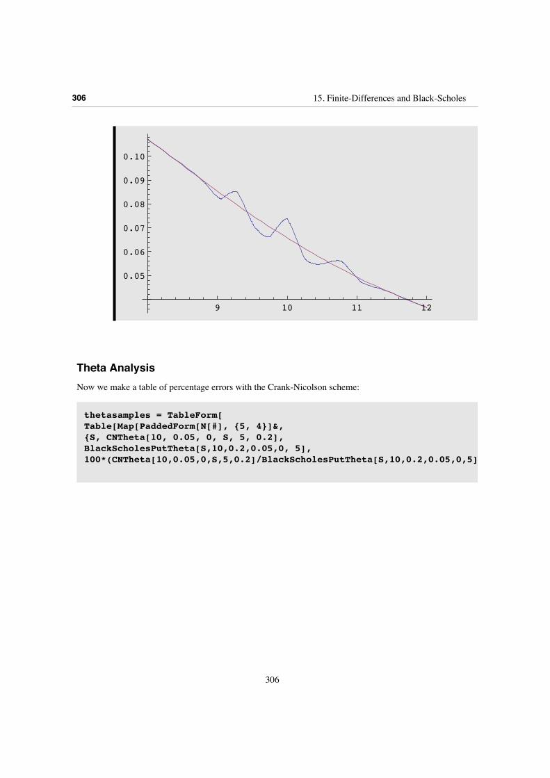
Theta AnalysisNow we make a table of percentage errors with the Crank-Nicolson scheme:
thetasamples = TableForm[Table[Map[PaddedForm[N[#], {5, 4}]&, {S, CNTheta[10, 0.05, 0, S, 5, 0.2],BlackScholesPutTheta[S,10,0.2,0.05,0, 5],100*(CNTheta[10,0.05,0,S,5,0.2]/BlackScholesPutTheta[S,10,0.2,0.05,0,5]-1)}], {S, 2, 16, 1}]]
306 15. Finite-Differences and Black-Scholes
306
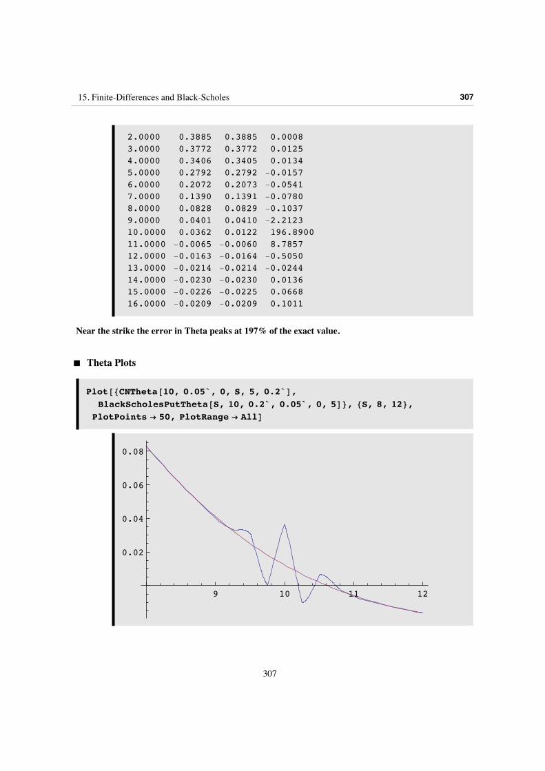
2.0000 0.3885 0.3885 0.00083.0000 0.3772 0.3772 0.01254.0000 0.3406 0.3405 0.01345.0000 0.2792 0.2792 -0.01576.0000 0.2072 0.2073 -0.05417.0000 0.1390 0.1391 -0.07808.0000 0.0828 0.0829 -0.10379.0000 0.0401 0.0410 -2.212310.0000 0.0362 0.0122 196.890011.0000 -0.0065 -0.0060 8.785712.0000 -0.0163 -0.0164 -0.505013.0000 -0.0214 -0.0214 -0.024414.0000 -0.0230 -0.0230 0.013615.0000 -0.0226 -0.0225 0.066816.0000 -0.0209 -0.0209 0.1011
Near the strike the error in Theta peaks at 197% of the exact value.
‡ Theta Plots
Plot@8CNTheta@10, 0.05`, 0, S, 5, 0.2`D,BlackScholesPutTheta@S, 10, 0.2`, 0.05`, 0, 5D<, 8S, 8, 12<,
PlotPoints Ø 50, PlotRange Ø AllD
9 10 11 12
0.02
0.04
0.06
0.08
Remark on Two-Time-Level Douglas
15. Finite-Differences and Black-Scholes 307
307
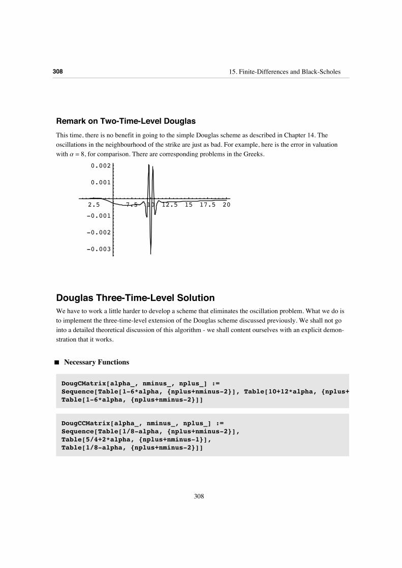
Remark on Two-Time-Level DouglasThis time, there is no benefit in going to the simple Douglas scheme as described in Chapter 14. The oscillations in the neighbourhood of the strike are just as bad. For example, here is the error in valuation with a = 8, for comparison. There are corresponding problems in the Greeks.
2.5 7.5 10 12.5 15 17.5 20
-0.003
-0.002
-0.001
0.001
0.002
Douglas Three-Time-Level SolutionWe have to work a little harder to develop a scheme that eliminates the oscillation problem. What we do is to implement the three-time-level extension of the Douglas scheme discussed previously. We shall not go into a detailed theoretical discussion of this algorithm - we shall content ourselves with an explicit demon-stration that it works.
‡ Necessary Functions
DougCMatrix[alpha_, nminus_, nplus_] :=Sequence[Table[1-6*alpha, {nplus+nminus-2}], Table[10+12*alpha, {nplus+nminus-1}],Table[1-6*alpha, {nplus+nminus-2}]]
DougCCMatrix[alpha_, nminus_, nplus_] :=Sequence[Table[1/8-alpha, {nplus+nminus-2}], Table[5/4+2*alpha, {nplus+nminus-1}],Table[1/8-alpha, {nplus+nminus-2}]]
308 15. Finite-Differences and Black-Scholes
308
DougDMatrix[alpha_, vec_List] := Module[{temp},temp = (10 - 12*alpha)*vec + (1+6*alpha)*(RotateRight[vec] + RotateLeft[vec]);temp[[1]] = Simplify[First[temp] - !(1+6*alpha)*Last[vec]];temp[[-1]] = Simplify[Last[temp] - (1 + 6*alpha)*First[vec]];temp]
DougDDMatrix[vec_List] := Module[{temp},temp = (10*vec + RotateRight[vec] + RotateLeft[vec]);temp[[1]] = Simplify[First[temp] - Last[vec]];temp[[-1]] = Simplify[Last[temp] - First[vec]];temp/6]
Douglas Three Time-Level Solution EvolutionThe initialization consists of defining the grid parameters, setting boundary and initial conditions and defining the various matrices.
dx = 0.025;dtau = 0.005;alpha = dtau/dx^2;M=20;nminus = 160;nplus = 160;alpha
8.
initial = Table@PutExercise@Hk - 1 - nminusL dx, 0.05, 0, 0.2D,8k, nminus + nplus + 1<D;
lower = Table@f@-nminus dx, Hm - 1L dtau, 0.05, 0, 0.2D, 8m, 1, M + 1<D;upper = Table@g@+nplus dx, Hm - 1L dtau, 0.05, 0, 0.2D, 8m, 1, M + 1<D;
w = Table[0, {m, 1, 3}, {k, 1, nminus+nplus+1}];
vold = Take[initial, {2, -2}];
15. Finite-Differences and Black-Scholes 309
309
w[[1,1]] = f[-nminus*dx, dtau/4, 0.05, 0, 0.2];w[[1, nminus+nplus+1]] = g[nplus*dx, dtau/4, 0.05, 0, 0.2];w[[2,1]] = f[-nminus*dx, dtau/2, 0.05, 0, 0.2];w[[2, nminus+nplus+1]] = g[nplus*dx, dtau/2, 0.05, 0, 0.2];w[[3,1]] = f[-nminus*dx, dtau, 0.05, 0, 0.2];w[[3, nminus+nplus+1]] = g[nplus*dx, dtau, 0.05, 0, 0.2];
CMat = DougCMatrix[alpha,nminus,nplus];CCMat = DougCCMatrix[alpha,nminus,nplus];
CMatQ = DougCMatrix[alpha/4,nminus,nplus];CMatH = DougCMatrix[alpha/2,nminus,nplus];
CCMatQ = DougCCMatrix[alpha/4,nminus,nplus];CCMatH = DougCCMatrix[alpha/2,nminus,nplus];
‡ Kick-Off Phase
This begins with the simple Douglas scheme with two time-levels and 1/4 the basic time-step.
rhs = DougDMatrix[alpha/4, vold]+Table[Which[k==1, (6*alpha/4+1)*lower[[1]] + (6*alpha/4-1)*w[[1, 1]],k== nplus + nminus-1, (6*alpha/4+1)*upper[[1]] +(6*alpha/4-1)*w[[1, nplus+nminus+1]],True, 0],{k, 1, nplus + nminus-1}];vnew = CompTridiagSolve[CMatQ, rhs];w[[1]] = Join[{w[[1,1]]}, vnew, {w[[1,nplus+nminus+1]]}];vvold = vold;vold = vnew;
Now we have two iterations of the three-time-level Douglas system, doubling the time-step at each stage:
310 15. Finite-Differences and Black-Scholes
310
rhs = DougDDMatrix[vold] - DougDDMatrix[vvold]/4 + Table[Which[k==1, (alpha/4-1/8)*w[[2, 1]] + w[[1,1]]/6 - lower[[1]]/24,k==nplus + nminus-1, (alpha/4-1/8)*w[[2, nplus+nminus+1]] + w[[1,nplus+nminus+1]]/6 - upper[[1]]/24,True, 0],{k, 1, nplus + nminus-1}];vnew = CompTridiagSolve[CCMatQ, rhs];w[[2]] = Join[{w[[2,1]]}, vnew, {w[[2,nplus+nminus+1]]}];vold = vnew;
rhs = DougDDMatrix[vold] - DougDDMatrix[vvold]/4 + Table[Which[k==1, (alpha/2-1/8)*w[[3, 1]] + w[[2,1]]/6 - lower[[1]]/24,k==nplus + nminus-1, (alpha/2-1/8)*w[[3, nplus+nminus+1]] + w[[2,nplus+nminus+1]]/6 - upper[[1]]/24,True, 0],{k, 1, nplus + nminus-1}];vnew = CompTridiagSolve[CCMatH, rhs];w[[3]] = Join[{w[[3,1]]}, vnew, {w[[3,nplus+nminus+1]]}];wold = initial;wvold = initial;wnew = w[[3]];
15. Finite-Differences and Black-Scholes 311
311
‡ Main Evolution Phase and Interpolation of Solution
For[m=3, m<=M+1, m++,(wvold = wold;wold = wnew;rhs = DougDDMatrix[Take[wold, {2, -2}]] -DougDDMatrix[Take[wvold, {2, -2}]]/4 + Table[Which[k==1, (alpha-1/8)*lower[[m]] + lower[[m-1]]/6 - lower[[m-2]]/24,k==nplus + nminus-1, (alpha-1/8)*upper[[m]] + upper[[m-1]]/6 - upper[[m-2]]/24,True, 0],{k, 1, nplus + nminus-1}];temp = CompTridiagSolve[CCMat, rhs];wnew = Join[{lower[[m]]}, temp, {upper[[m]]}])]
points = Table@Hk - nminus - 1L * dx,8k, 1, nplus + nminus + 1<D;
finalstep = wnew;
prevstep = wold;
pprevstep = wvold;
interpoldata = Transpose@8points, finalstep<D;
ufunc = Interpolation[interpoldata, InterpolationOrder -> 3];
Valuation[strike_, r_, q_, S_, T_, sd_] :=ValuationMultiplier[strike, r, q, Log[S/strike], sd^2*T/2, sd]*ufunc[Log[S/strike]]
Valuation Analysis
312 15. Finite-Differences and Black-Scholes
312
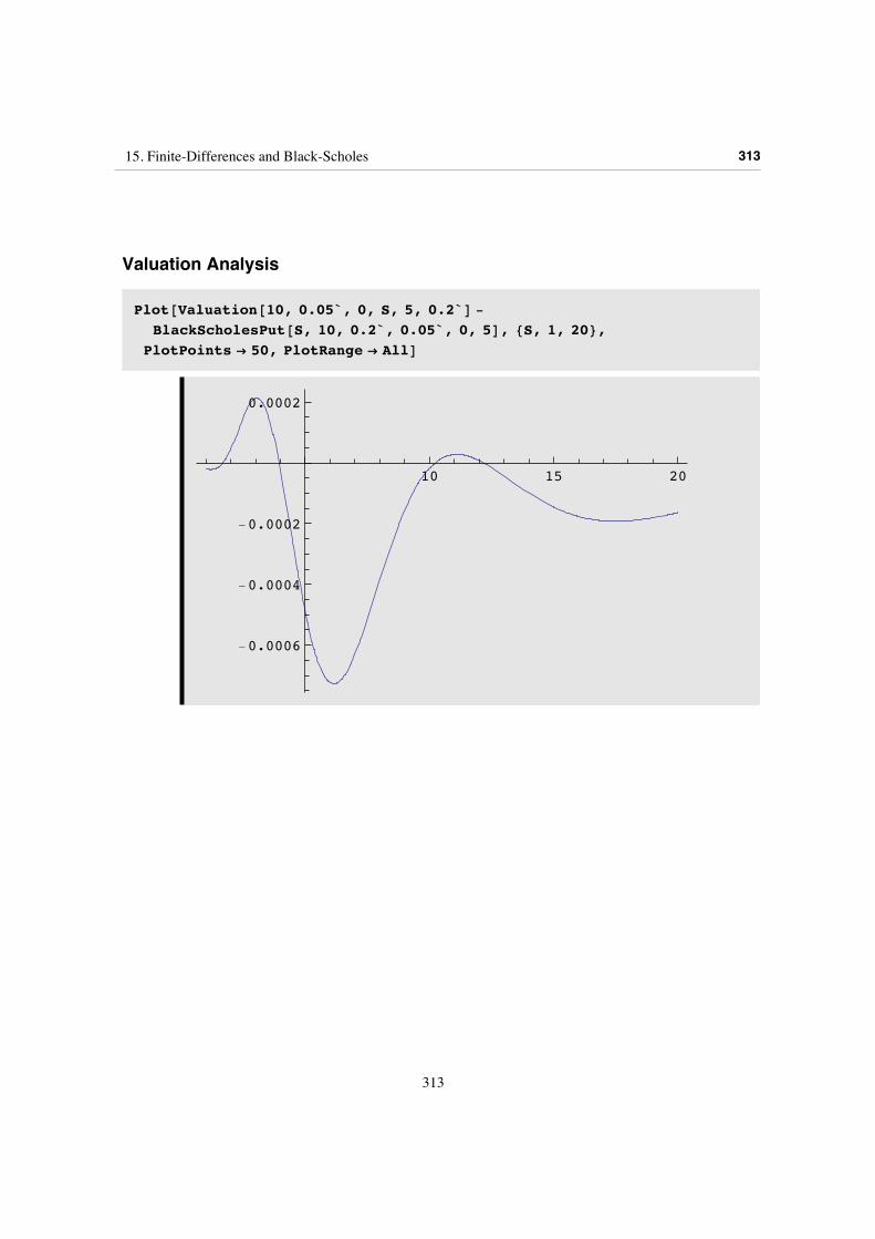
Valuation Analysis
Plot@Valuation@10, 0.05`, 0, S, 5, 0.2`D -
BlackScholesPut@S, 10, 0.2`, 0.05`, 0, 5D, 8S, 1, 20<,PlotPoints Ø 50, PlotRange Ø AllD
10 15 20
-0.0006
-0.0004
-0.0002
0.0002
15. Finite-Differences and Black-Scholes 313
313
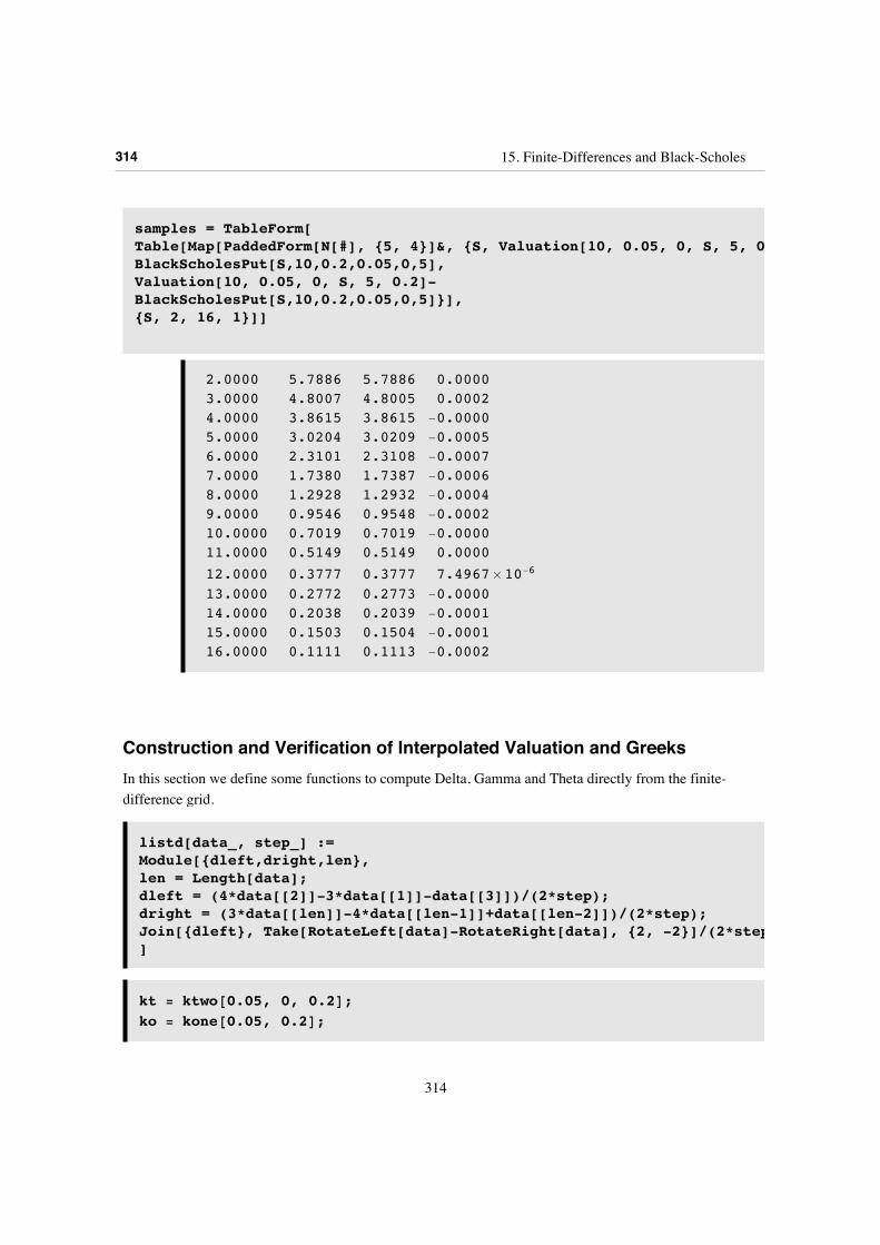
samples = TableForm[Table[Map[PaddedForm[N[#], {5, 4}]&, {S, Valuation[10, 0.05, 0, S, 5, 0.2],BlackScholesPut[S,10,0.2,0.05,0,5],Valuation[10, 0.05, 0, S, 5, 0.2]-BlackScholesPut[S,10,0.2,0.05,0,5]}],{S, 2, 16, 1}]]
2.0000 5.7886 5.7886 0.00003.0000 4.8007 4.8005 0.00024.0000 3.8615 3.8615 -0.00005.0000 3.0204 3.0209 -0.00056.0000 2.3101 2.3108 -0.00077.0000 1.7380 1.7387 -0.00068.0000 1.2928 1.2932 -0.00049.0000 0.9546 0.9548 -0.000210.0000 0.7019 0.7019 -0.000011.0000 0.5149 0.5149 0.000012.0000 0.3777 0.3777 7.4967 µ 10-6
13.0000 0.2772 0.2773 -0.000014.0000 0.2038 0.2039 -0.000115.0000 0.1503 0.1504 -0.000116.0000 0.1111 0.1113 -0.0002
Construction and Verification of Interpolated Valuation and GreeksIn this section we define some functions to compute Delta, Gamma and Theta directly from the finite-difference grid.
listd[data_, step_] :=Module[{dleft,dright,len},len = Length[data];dleft = (4*data[[2]]-3*data[[1]]-data[[3]])/(2*step);dright = (3*data[[len]]-4*data[[len-1]]+data[[len-2]])/(2*step);Join[{dleft}, Take[RotateLeft[data]-RotateRight[data], {2, -2}]/(2*step), {dright}]]
kt = [email protected], 0, 0.2D;ko = [email protected], 0.2D;
314 15. Finite-Differences and Black-Scholes
314
deltadata = listd@finalstep, dxD -1
2Hkt - 1L finalstep;
gammadata = listd@deltadata, dxD -1
2Hkt + 1L deltadata;
thetadata =3 finalstep - 4 prevstep + pprevstep
2 dtau-
1
4Hkt - 1L2 + ko finalstep;
deltainterpoldata = Transpose@8points, deltadata<D;gammainterpoldata = Transpose@8points, gammadata<D;thetainterpoldata = Transpose@8points, thetadata<D;
dfunc = Interpolation@deltainterpoldata, InterpolationOrder Ø 3D;gfunc = Interpolation@gammainterpoldata, InterpolationOrder Ø 3D;tfunc = Interpolation@thetainterpoldata, InterpolationOrder Ø 3D;
DougDelta@strike_, r_, q_, S_, T_, sd_D :=
1
SValuationMultiplierBstrike, r, q, LogB
S
strikeF,
sd2 T
2, sdF
dfuncBLogBS
strikeFF
DougGamma@strike_, r_, q_, S_, T_, sd_D :=
1
S2ValuationMultiplierBstrike, r, q, LogB
S
strikeF,
sd2 T
2, sdF
gfuncBLogBS
strikeFF
15. Finite-Differences and Black-Scholes 315
315
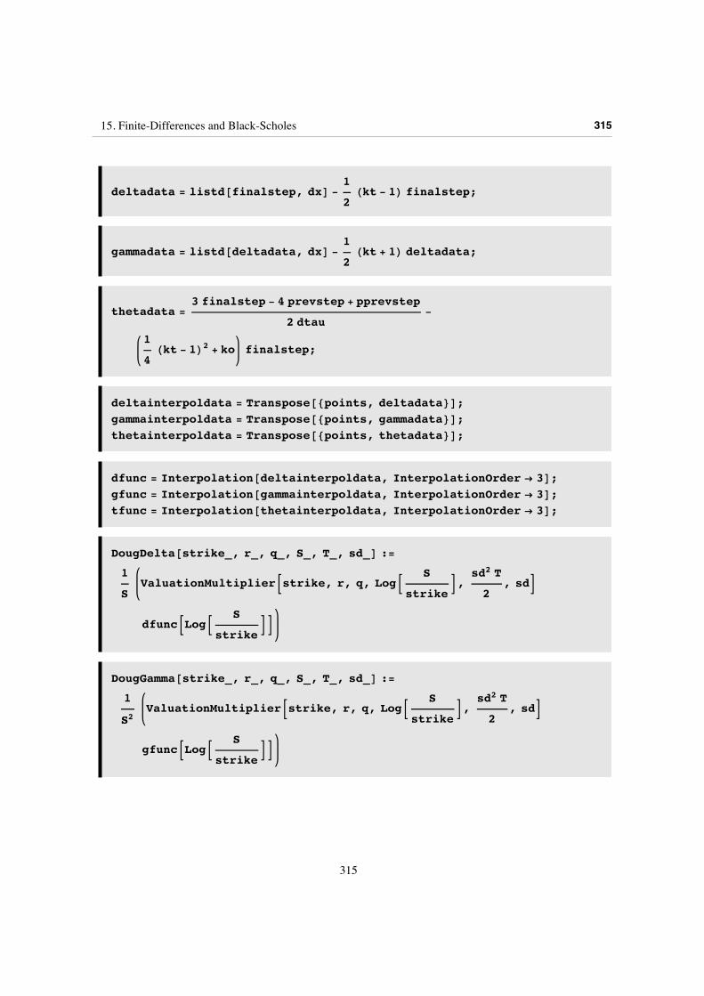
DougTheta@strike_, r_, q_, S_, T_, sd_D :=
-1
2sd2 ValuationMultiplierBstrike, r, q, LogB
S
strikeF,
sd2 T
2, sdF
tfuncBLogBS
strikeFF
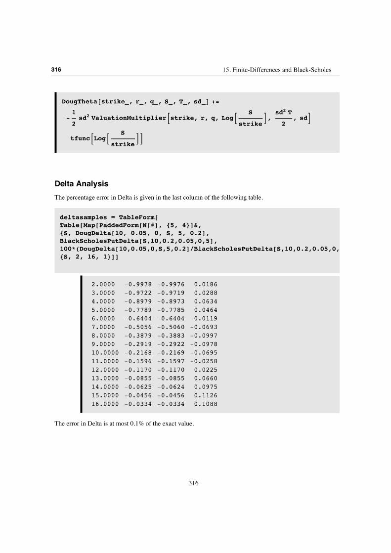
Delta AnalysisThe percentage error in Delta is given in the last column of the following table.
deltasamples = TableForm[Table[Map[PaddedForm[N[#], {5, 4}]&, {S, DougDelta[10, 0.05, 0, S, 5, 0.2],BlackScholesPutDelta[S,10,0.2,0.05,0,5],100*(DougDelta[10,0.05,0,S,5,0.2]/BlackScholesPutDelta[S,10,0.2,0.05,0,5]-1)}],{S, 2, 16, 1}]]
2.0000 -0.9978 -0.9976 0.01863.0000 -0.9722 -0.9719 0.02884.0000 -0.8979 -0.8973 0.06345.0000 -0.7789 -0.7785 0.04646.0000 -0.6404 -0.6404 -0.01197.0000 -0.5056 -0.5060 -0.06938.0000 -0.3879 -0.3883 -0.09979.0000 -0.2919 -0.2922 -0.097810.0000 -0.2168 -0.2169 -0.069511.0000 -0.1596 -0.1597 -0.025812.0000 -0.1170 -0.1170 0.022513.0000 -0.0855 -0.0855 0.066014.0000 -0.0625 -0.0624 0.097515.0000 -0.0456 -0.0456 0.112616.0000 -0.0334 -0.0334 0.1088
The error in Delta is at most 0.1% of the exact value.
316 15. Finite-Differences and Black-Scholes
316
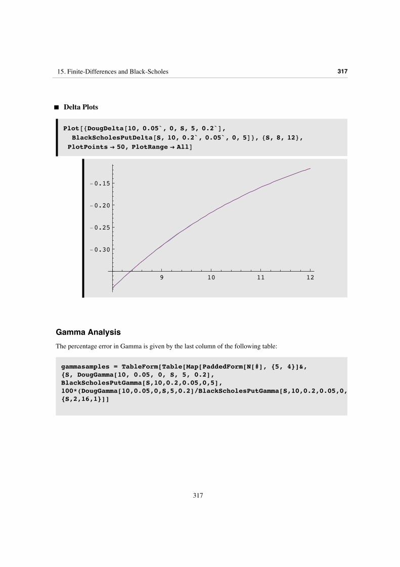
‡ Delta Plots
Plot@8DougDelta@10, 0.05`, 0, S, 5, 0.2`D,BlackScholesPutDelta@S, 10, 0.2`, 0.05`, 0, 5D<, 8S, 8, 12<,
PlotPoints Ø 50, PlotRange Ø AllD
9 10 11 12
-0.30
-0.25
-0.20
-0.15
Gamma AnalysisThe percentage error in Gamma is given by the last column of the following table:
gammasamples = TableForm[Table[Map[PaddedForm[N[#], {5, 4}]&, {S, DougGamma[10, 0.05, 0, S, 5, 0.2],BlackScholesPutGamma[S,10,0.2,0.05,0,5],100*(DougGamma[10,0.05,0,S,5,0.2]/BlackScholesPutGamma[S,10,0.2,0.05,0,5]-1)}],{S,2,16,1}]]
15. Finite-Differences and Black-Scholes 317
317
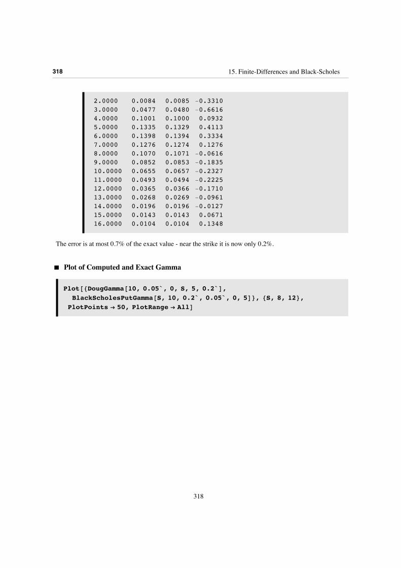
2.0000 0.0084 0.0085 -0.33103.0000 0.0477 0.0480 -0.66164.0000 0.1001 0.1000 0.09325.0000 0.1335 0.1329 0.41136.0000 0.1398 0.1394 0.33347.0000 0.1276 0.1274 0.12768.0000 0.1070 0.1071 -0.06169.0000 0.0852 0.0853 -0.183510.0000 0.0655 0.0657 -0.232711.0000 0.0493 0.0494 -0.222512.0000 0.0365 0.0366 -0.171013.0000 0.0268 0.0269 -0.096114.0000 0.0196 0.0196 -0.012715.0000 0.0143 0.0143 0.067116.0000 0.0104 0.0104 0.1348
The error is at most 0.7% of the exact value - near the strike it is now only 0.2%.
‡ Plot of Computed and Exact Gamma
Plot@8DougGamma@10, 0.05`, 0, S, 5, 0.2`D,BlackScholesPutGamma@S, 10, 0.2`, 0.05`, 0, 5D<, 8S, 8, 12<,
PlotPoints Ø 50, PlotRange Ø AllD
318 15. Finite-Differences and Black-Scholes
318
9 10 11 12
0.05
0.06
0.07
0.08
0.09
0.10
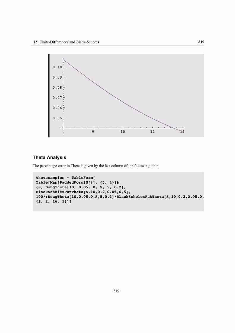
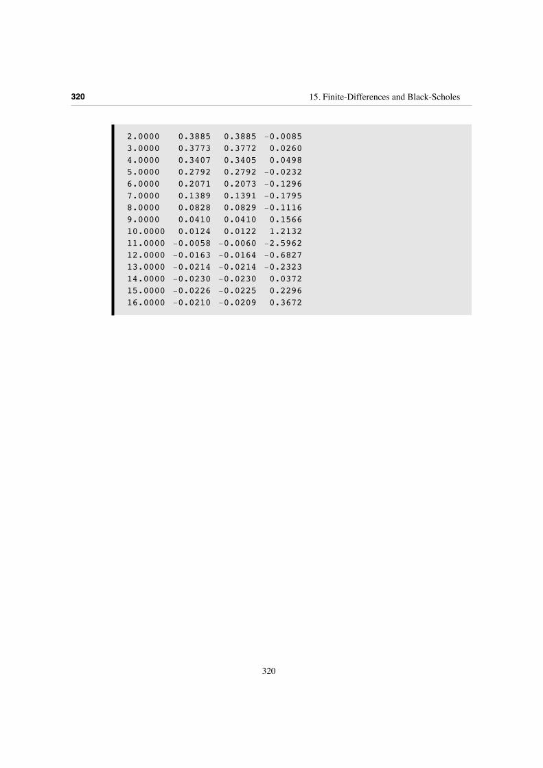
Theta AnalysisThe percentage error in Theta is given by the last column of the following table:
thetasamples = TableForm[Table[Map[PaddedForm[N[#], {5, 4}]&, {S, DougTheta[10, 0.05, 0, S, 5, 0.2],BlackScholesPutTheta[S,10,0.2,0.05,0,5],100*(DougTheta[10,0.05,0,S,5,0.2]/BlackScholesPutTheta[S,10,0.2,0.05,0,5]-1)}],{S, 2, 16, 1}]]
15. Finite-Differences and Black-Scholes 319
319
2.0000 0.3885 0.3885 -0.00853.0000 0.3773 0.3772 0.02604.0000 0.3407 0.3405 0.04985.0000 0.2792 0.2792 -0.02326.0000 0.2071 0.2073 -0.12967.0000 0.1389 0.1391 -0.17958.0000 0.0828 0.0829 -0.11169.0000 0.0410 0.0410 0.156610.0000 0.0124 0.0122 1.213211.0000 -0.0058 -0.0060 -2.596212.0000 -0.0163 -0.0164 -0.682713.0000 -0.0214 -0.0214 -0.232314.0000 -0.0230 -0.0230 0.037215.0000 -0.0226 -0.0225 0.229616.0000 -0.0210 -0.0209 0.3672
320 15. Finite-Differences and Black-Scholes
320
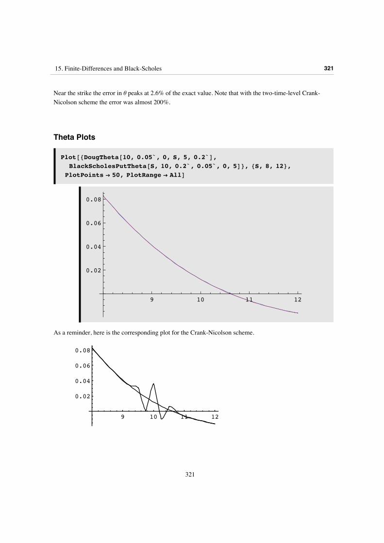
Near the strike the error in q peaks at 2.6% of the exact value. Note that with the two-time-level Crank-Nicolson scheme the error was almost 200%.
Theta Plots
Plot@8DougTheta@10, 0.05`, 0, S, 5, 0.2`D,BlackScholesPutTheta@S, 10, 0.2`, 0.05`, 0, 5D<, 8S, 8, 12<,
PlotPoints Ø 50, PlotRange Ø AllD
9 10 11 12
0.02
0.04
0.06
0.08
As a reminder, here is the corresponding plot for the Crank-Nicolson scheme.
9 10 11 12
0.02
0.04
0.06
0.08
Summary
15. Finite-Differences and Black-Scholes 321
321
SummaryThe introduction of implicit schemes is motivated by the desire to get accurate and stable solutions for larger values of a. When we need to compute the values of both a function and its first and second derivatives, popular schemes such as the ordinary two-time-level Crank-Nicolson scheme are unsuitable for option-pricing problems, unless small to moderate values of a are used. This is because of the fact that non-smoothness in initial data (almost always present in option payoffs) propagates through the solution causing small oscillatory errors. When amplified by the process of differentiation, these may cause substantial errors in the Greeks. The errors in the valuation may be deceptively small - to quote Wilmott et al (1993) when discussing a verification example with the Crank-Nicolson scheme, they remark that "Even with a = 10, the numerical and exact results differ only marginally." This is absolutely right, at least when we just look at the valuation. When we inspect the Greeks a rather more disturbing picture emerges. We have given an example where estimates of q from a computation with a = 8 are in error by about 200%.
The oscillation problem and the resulting corruption of the Greeks can be cured by the use of a more suitable difference scheme. When the initial data were smooth, we saw previously that the two-time-level Douglas scheme was sufficient, but in the presence of non-smooth data the corresponding three-time-level Douglas scheme cures the problems quite dramatically.
The transition to such a scheme for practitioners should not be a great leap. We have already seen that the two-time-level Douglas scheme is the natural implicit generalization of the trinomial model, when carried out on a grid rather than a tree. The next step to a three-time-level scheme allows larger time steps still to be taken without a loss of accuracy or corruption of the Greeks.
322 15. Finite-Differences and Black-Scholes
322