Finite Element Analysis and Statistical Method to Determine Temperature Distribution on Cutting

European Journal of Scientific Research ISSN 1450-216X Vol.30 No.3 (2009), pp.451-463 © EuroJournals Publishing, Inc. 2009 http://www.eurojournals.com/ejsr.htm

Finite Element Analysis and Statistical Method to Determine

Temperature Distribution on Cutting Tool in End-Milling

K. Kadirgama Faculty of Mechanical Engineering, Universiti Malaysia Pahang

Tun Abdul Razak Highway, 26300 Gambang, Kuantan, Pahang, Malaysia E-mail: [email protected]

M.M. Noor

Faculty of Mechanical Engineering, Universiti Malaysia Pahang Tun Abdul Razak Highway, 26300 Gambang, Kuantan, Pahang, Malaysia

E-mail: [email protected]

M.M. Rahman Faculty of Mechanical Engineering, Universiti Malaysia Pahang


Tel: +6095492207; Fax: +6095492244

W.S.W. Harun Faculty of Mechanical Engineering, Universiti Malaysia Pahang


C.H.C. Haron

Department of Mechanical and Materials Engineering Faculty of Engineering and Built Environment

Universiti Kebangsaan Malaysia 43600 Bangi, Selangor, Malaysia

E-mail: [email protected]

Abstract

The aim of this study is to determine the temperature distribution on cutting tool when machining HASTELLOY C-22HS with carbide coated cutting tool. Response Surface Method (RSM) used to minimize the number of experiments and to develop first order temperature model. Finite element analysis (FEA) was used to verification of the temperature distribution on cutting tool. From FEA results show clearly that the relationship between the variables (cutting speed, feed rate and axial depth) with responses (temperature). From the first order model shows that cutting speed, feed rate and axial depth plays important role in producing cutting temperature. The feed rate has the most dominant parameter on the temperature, followed by the axial depth and cutting speed. The results from FEA were compared with the experimental values. The predicted values are quite close to the experimental results, even though its accuracy is slightly inferior as

Finite Element Analysis and Statistical Method to Determine Temperature Distribution on Cutting Tool in End-Milling 452

compared to RSM. However, FEA is able to produce the temperature distribution around the cutting tool, in great detail. The predicted values deviate slightly from the experimental values due to the employed friction value. Keywords: Finite element analysis, temperature, end-milling, response surface method,

HASTELLOY C-22HS. 1. Introduction Modern machining processes face continuous cost pressures and high quality expectations. To remain competitive a company must continually identify cost reduction opportunities in production, exploit economic opportunities, and continuously improve production processes. A key technology that represents cost saving opportunities related to improve the overall performance of cutting operations. The metal cutting is a coupled of thermo-mechanical process. During the process, the heat generation occurs as a result of plastic deformation and friction along the tool–chip and tool–workpiece interface. It is a comprehensive assumption that almost all the energy required for cutting is converted to heat in the cutting domain. The temperature rises to critical levels up to 1000 ◦C in the cutting zone affecting the material behavior and mechanics of chip formation. The maximum temperature occurs at the tool–chip interface. The tool–wear and fracture considerably increase at higher temperatures. Temperature rise in machining has a controlling influence on the cutting parameters. Many parameters depend on the temperature field during cutting: tool life, mechanics of chip formation, surface quality, cutting forces, cutting speed, process efficiency, etc. Determination of temperature distribution in cutting domain, therefore, has been one of the major subjects in the machining researches [1]. Usui and Shirakachi [2] have first assumed the shear cutting angle, chip geometry and flow line in order to predict parameters such as stress, strain and temperature. Fang et al. [3] have included the effect of adhering layer formation on the tool into the finite element analysis. The temperature gradient vertical to the rake face is smaller as compared to that of the adhering layer. Ng et al. [4] was employed the finite element method to calculate the cutting force and temperature distribution. The authors were used the experimental data obtained from the infrared and cutting force measurements in order to validate their model. At lower heat conductance, the amount of heat carried by the chip and the temperature of the tool–chip interface is higher. Muraka et al. [5] have studied the influence of process variables such as cutting speed, feed rate, rake angle, flank wear rate, coolant water on the temperature distribution. Along the tool-chip interface, the highest temperature point has been found to move towards the end of the contact length with the increase of cutting speed and feed rate. When the cutting edge is not sharp enough, metal is pushed instead of cut, results in higher cutting force and higher temperature [6].

A lot of efforts have been made to measure the temperatures at the tool-chip interface zone, chip, cutting tool and the workpiece. A review of the common experimental techniques designed for temperature measurement in metal cutting processes reveals that these techniques can be classified as: direct conduction, indirect radiation, and metallographic. These techniques have been reviewed by Da Silva and Wallbank [7], Ay and Yang [8] and more recently by Komanduri and Hou [9], O’Sullivan and Cotterell [10], and Sutter et al. [11]. Generally, these techniques include: tool-work thermocouple, embedded thermocouple, radiation pyrometer, metallographic technique and a method of using powders of constant melting point. Maekawa et al. [12] have employed this technique to study the effect of cutting temperature on tool wear in high speed turning operation of Inconel 718 and milling operation of Ti-6Al-6V-2Sn alloy. Tungsten micro-thermocouples are embedded in the tool. Temperatures of 1200 ºC and 1100 ºC are reported for the ceramic–Inconel tool material pair at 150 m/min and the carbide-Ti-6Al-6V-2Sn tool-material pair at 500 m/min, respectively. Chen et al. [13] have calculated the heat flowing into the rake face of the cutting tool by using the Inverse Heat

453 K. Kadirgama, M.M. Noor, M.M. Rahman, W.S.W. Harun and C.H.C. Haron

Conduction Method (IHCM), based on the interior temperatures measured from a thermocouple. Although this technique has been widely used, especially for the estimation of temperature of the tool, there are a number of limitations and questionable aspects concerning on the placement of the thermocouple. It is due to the fact that the thermocouples alter the heat flow, as well as, limit the strength of the tool. Other limitations include the slow response time, difficulty in drilling holes on hard material such as ceramics, as well as, its inability to predict the transient response of temperature.

The radiation techniques are non-contact thermographic methods designed to measure the surface temperature of a body based on its emitted thermal energy. It is available for temperature field measurement (infrared thermography), including photo camera with films sensitive to infrared radiation and infrared camera, and for temperature point measurement (infrared pyrometer). The radiation technique has many advantages over the thermo-electric technique: (i) faster response; (ii) no adverse effects on temperature and material; (iii) no physical contact; and (iv) allowing measurements on objects that are difficult to access. This technique is probably the most suitable in HSM applications where high temperature can be captured easily as there is no direct contact taking place with the heat source. However, the measurement position must be selected carefully as the accuracy can be significantly affected by chip obstruction. Chip obstruction also causes the temperature measurement difficult to be performed, especially those taking place at the toolchip interface. In addition, the exact surface emissivity must be known as it strongly affects the measured temperature. O’Sullivan and Cotterell [10] have applied a coating of known emissivity on the workpiece surface in order to eliminate any measurement problems. There are many values of emissivity reported in literature for different cutting tools and workpiece materials. However, it is important to note that the emissivities of most metals with clean surface or thin oxide layer vary with wavelength and temperature. Therefore, the pyrometeroperating wavelength and band data must match with the spectral emissivity values. In addition, emissivity measurement is also complicated by the fact that the emissivity of an object alters significantly with respect to the change of surface condition such as oxidation, etc. In most cases, in order to overcome the uncertainty of the emissivity measurement, it is important to measure the emissivity of the object prior to the temperature measurement performed in the cutting test. Yourong et al. [14] have used the infrared camera to investigate the temperature distribution on the flank face of ceramic tools used for turning operation. More recently, Muller and Renz [15] have developed a two-colour fiber-optic pyrometer for the measurement of temperatures on surfaces of unknown or varying emissivity. The pyrometer has been also used for the temperature measurement of the chip and the workpiece in an oblique turning process of AISI 1045 steel. Infra-red (IR) pyrometer has been used as a remote sensor to measure the temperature at the tool-chip interface in high-speed milling operation [16]. The measured temperatures have been used as an input for the inverse heat transfer model to calculate the heat flux and temperature distribution on the tool-chip interface.

In metallographic techniques, the temperature measurement involves the analysis of the microstructure or the microhardness of the heat-affected zone within the cutting tool. It requires calibration curves, which give the hardness of the tool material against the known temperatures and heating time. Typically the accuracy of the temperatures measured by this method is in the range of G25 8C. However, this technique is mainly limited to HSS tools, which experience a change of the structure/microhardness with temperature in the range from 600 to 1000 oC. It has been reported that temperature maps can be constructed for the iron-bonded cemented carbide tools where cobalt is replaced by iron [17]. The accuracy of this method to determine the metal cutting temperature is limited. This method cannot be used to record the temperature field in the cutting tool as a function of time. The fine powder method can be used to predict the temperature gradients on the rake face of cutting tools. The temperature distribution on the rake face is estimated by observing the boundary line formed by the melted and unmelted powder scattered on the tool surface. The complexity of the machining process makes it extremely difficult to compare the results obtained from different techniques. In terms of the temporal and spatial resolutions of the temperature measurement performed in metal cutting operation, it has been reported that the best temporal resolution of 50 mm can be obtained by the pyrometer while the best spatial resolution of 5 mm can be obtained by thermal video

Finite Element Analysis and Statistical Method to Determine Temperature Distribution on Cutting Tool in End-Milling 454 cameras [18]. The objective of this study is to determine the temperature distribution on cutting tool while the machining the Hastelloy C-22 HS and also develop the statistical model to predict the temperature profile using the FEA. 2. Response Surface Method Response surface method is found the successful technique to perform the trend analysis of surface roughness with respect to various combinations of design variables include the cutting speed, feed rate, axial depth and radial depth [19]. It is a combination of experimental and regression analysis and statistical inferences. The concept of the response surface involves a dependent variable (y) called the response variable and several independent variables x1, x2,...,xk. If all of these variables are assumed to be measurable, the response surface can be expressed as Eq. (1).

y = f (x1, x2,... xk) (1) The goal is to optimize the response variable y. It is assumed that the independent variables are

continuous and controllable by the experimenter with negligible error. The response or the dependent variable is assumed to be a random variable. Say in a milling operation, it is necessary to find a suitable combination of cutting speed (x1 = ln V), feed (x2 = ln f), axial depth (x3 = ln ax) and radial depth(x4 = ln ar) that optimize response. The observed response y as a function of the speed, feed, axial depth and radial depth can be written as in Eq. (2).

Cqpnmy +×+×+×+×= depth Radialdepth Axialrate Feedspeed Cutting (2) where y is the response, C, m, n, p and q are the constants. Equation (2) can also be expressed as in Eq. (3):

4433221100 xxxxxy βββββ ++++= (3) where y is the response, x0 = 1(dummy variables), x1= cutting speed, x2 = feed rate, x3 = axial depth and x4 = radial depth. β0 = C and β1, β2, β3, and β4 are the model parameters.

El-Khabeery and Fattouh [20] was studied the residual stresses based on a moving heat source under various simulated cutting conditions, but the predicted trend was not in agreement with the results of actual machining. RSM was then utilized to determine the residual stresses under different cutting conditions and for various tensile strengths presented by different materials [21]. Whilst the properties of the materials were not coincident except for tensile strength, some materials machined by a tool with a chamfer have been found to result in microstructure change because of temperature effect. Alauddin et al. [22] proposed a prediction models by using the Takushi method and RSM by using factors such as cutting speed, feed and depth of cut. 2.1. Box-Behnken Design

Box-Behnken Design is normally used when performing non-sequential experiments that are performing the experiment only once. These designs allow efficient estimation of the first and second-order coefficients. Because Box-Behnken design has fewer design points, they are less expensive to run than central composite designs with the same number of factors. Box-Behnken design do not have axial points, thus can be sure that all design points fall within the safe operating. Box-Behnken design also ensures that all factors never set at their high levels simultaneously [23]. After the preliminary investigation, the suitable levels of the factors were used to deduce the design parameters. Level of independence variables are given in Table 1 and experimental design variables are shown in Table 2. In this study, 3 variables have been selected include the cutting speed, feed rate and axial depth. For the radial depth, 3.5 mm has been selected for every experiment.


Table 1: Level of Independence Variables

Levels Low Medium High Coding -1 0 1 Speed, v (m/min) 100 140 180 Feed rate, f (mm/rev) 0.1 0.15 0.2 Axial depth, da (mm) 1 1.5 2

Table 2: Experimental design

Cutting Speed (m/min) Feed Rate (mm/rev) Axial Depth (mm) 140 0.1 2 140 0.2 1 100 0.15 1 100 0.15 2 140 0.15 1.5 100 0.1 1.5 180 0.1 1.5 180 0.15 2 180 0.2 1.5 140 0.2 2 180 0.15 1 140 0.15 1.5 140 0.1 1 100 0.2 1.5 140 0.15 1.5

3. Finite Element Analysis Thirdwave Systems Advantedge is utilized for machining simulations. It is developed based on the dynamic explicit Lagrangian formulation. The model was built by selecting the type of machining operation of milling and defining the necessary process parameters. Since the main subject of this work is related to milling operation, the process parameters are feed rate, axial depth of cut, length of cut, radial depth, spindle speed and initial temperature of the workpiece. This model is thermo-mechanically coupled. In Advantedge, a staggered procedure is adopted for the purpose of coupling the thermal and mechanical equations. Geometrically identical meshes for the thermal and mechanical models are used. Mechanical and thermal computations are staggered, assuming constant temperature during the mechanical step and constant heat generation during the thermal step. A mechanical step is taken first based on the current distribution of temperature, and the heat generated is computed from plastic working and frictional heat generation. Certain assumptions are made to simulate the complex procedure of metal cutting with FEM. These assumptions are used to define the problem to be solved as well as to apply the boundary and loading conditions:

1. The cutting speed is constant. 2. The width of cut is larger than the feed (plane strain condition), and both are constant. 3. The cutting velocity vector is normal to the cutting edge. 4. The workpiece material is a homogeneous polycrystalline, isotropic, and incompressible solid. 5. The workpiece is set at a reference temperature of 20° C at the beginning of simulation. 6. The machine tool is perfectly rigid and no influence of machine tool dynamics on machining is

considered. 7. Constant friction at tool-chip interaction and tool-workpiece interaction.

The initial coolant temperature is selected as the room temperature. Heat flux due to coolant is applied to all exposed and non-contacting surfaces on tool and workpiece, except the bottom face of the workpiece and the faces on the tool where constant temperature is applied. The heat transfer coefficient of the coolant is 10000 W/ (m2.K) and the coolant temperature is 20ºC.

Finite Element Analysis and Statistical Method to Determine Temperature Distribution on Cutting Tool in End-Milling 456 4. Experimental Setup The 15 experiments were carried out on Okuma CNC machining centre MX-45 VA with 90º holders and using a standard coolant. The water soluble coolant was used in these experiments. Each experiment was stopped after 85 mm cutting length. For the temperature measurement on the tool tip Infrared Thermometer was used as shown in Figure 1. Each experiment was repeated three times using a new cutting edge every time to obtain accurate readings of the cutting force and temperature. A cutting pass was conducted in such a way that a shoulder, of depth ranging from 1 to 2 mm, and width 3.5 mm, was produced.

Figure 1: Infrared thermometer.

The workpiece material was selected to represent the major group of workpiece materials used in industry. The cutting tools used in this study are a 12º rake positive end milling cutter of 50 mm diameter. The end mill can be equipped with four inserts whose only one edge can be used for cutting. The tool inserts were made by Kennametal and had an ISO catalogue number of SPHX1205ZCFRGN1W (KC520M). KC520M is coated with TiAIN (PVD). In this study, only one inserts per one experiment was mounted on the cutter. 5. Results and Discussion After conducting the first pass (one pass is equal to 85 mm length) of the 15 cutting experiments, the cutting temperature readings are used to determine the parameters appearing in the postulated first-order model. In order to determine these parameters, the least square method is used with the aid of Minitab. The first-order linear equation to predicte the cutting temperature can be expressed in Eq. (4):

813256.031.16321+++=′ xxy (4)

From Eq. (4) can easily notice that the response y′ (cutting temperature) is affected significantly by feed rate followed by axial depth of cut and cutting speed for all the models. Generally, the increase in feed rate, axial depths and cutting speed causes the cutting temperature to increase [24]. Lee et al. [25] have also reported that the nickel-based alloy is high in strength due to the high temperature and stress at the tool-chip contact area. Although nickel-based alloys are not


exceptionally hard but their outstanding high temperature strength and extreme toughness create difficulties during machining due to their tendencies of work hardening, which result in very high cutting forces and significant burr formation during machining. Figure 2 shows the measured cutting temperature values and those predicted by the first-order model. It is clearly shows that the predicted values well agree with the experimental results. This indicates that the obtained linear model is useful to predict the cutting temperature. The adequacy of the first-order model is verified using the ANOVA. At a level of confidence of 95%, the model is checked for its adequacy. As shown in Table 3, the P value is not significant with the lack-of fit (<0.05). This implies that the model could fit and it is adequate [26-27].

Figure 2: Experiment result and prediction result for first order cutting temperature model 90º coolant and dry

0

100

200

300

400

500

600

700

1 2 3 4 5 6 7 8 9 10 11 12 13 14 15

No.Experiments

Tem

pera

ture

(deg

C)

Exp.Temperature(N)(90°-clt)

Pred.Temperature(N)(90° - clt)

Exp.Temperature(N)(90°-dry)

Pred.Temperature(N)(90° -dry)

Table 3: Variance analysis for first order cutting temperature model

Source Degree of Freedom F-ratio P-value Regression 3 9.57 0.002 Linear 3 9.57 0.002 Residual Error 11 Lack-of-Fit 9 2.29 0.341 Pure Error 2 Total 14

Large temperature difference occurred between the cutting edge and bulk of the insert causes

evenly spaced cracks perpendicular to the cutting edge. Interrupted cutting (as in milling), or machining materials such as nickel superalloys can cause temperature fluctuations. Cracks progress slowly, leading to chipping and eventually, tool fracture [25]. As shown in Figure 3, the coating layers are worn off due to the high temperature. It can be seen that from Figure 4, the chips from the workpiece are stuck on the cutting tool due to high temperature and this leads to tool failure.

Finite Element Analysis and Statistical Method to Determine Temperature Distribution on Cutting Tool in End-Milling 458

Figure 3: Coating layers are wearing off because of the high temperature.

The coating layer wears off

Figure 4: Chips from the workpiece already stuck at the cutting tool due to high temperature.

Chip stuck at insert

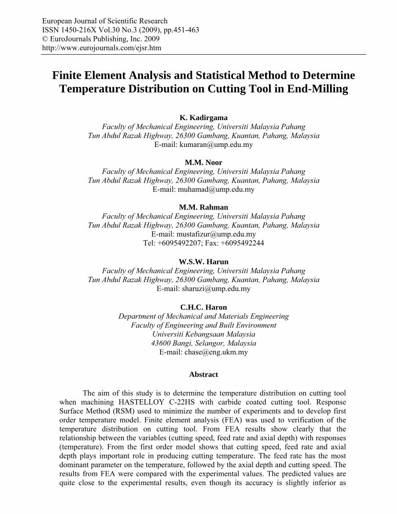
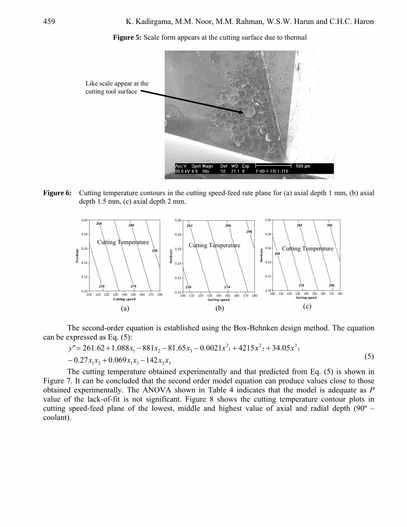
Heat and pressure generated in machining can cause the cutting tool’s binder to soften, allowing the carbide grains to move. Little insert material is actually worn away, as it is in crater wear, but the nose of the insert becomes distorted. Inconsistent part size and tool breakage can follow. As shown in Figure 5, scale form appears at the cutting surface due to thermal deformation. Figures 6 shows the cutting temperature contours at three different axial depths (lowest “-1”, middle “0”, and highest values “+1”). It is clear that an increase in all the variables cause the cutting temperature to increase dramatically.


Figure 5: Scale form appears at the cutting surface due to thermal

Like scale appear at the cutting tool surface

Figure 6: Cutting temperature contours in the cutting speed-feed rate plane for (a) axial depth 1 mm, (b) axial

depth 1.5 mm, (c) axial depth 2 mm.

Cutting speed

Feed

rate

298

286

274

262

250

180170160150140130120110100

0.20

0.18

0.16

0.14

0.12

0.10

Cutting speed

Feed

rate 290

280

270

260

250

180170160150140130120110100

0.20

0.18

0.16

0.14

0.12

0.10

Cutting speed

Feed

rate

300

290

280

270

260

180170160150140130120110100

0.20

0.18

0.16

0.14

0.12

0.10

(a) (b) (c)

Cutting Temperature Cutting Temperature Cutting Temperature

The second-order equation is established using the Box-Behnken design method. The equation can be expressed as Eq. (5):

323121

32

22

12

321

142069.027.005.3442150021.065.81881088.162.261"

xxxxxxxxxxxxy

−+−++−−−+=

(5)

The cutting temperature obtained experimentally and that predicted from Eq. (5) is shown in Figure 7. It can be concluded that the second order model equation can produce values close to those obtained experimentally. The ANOVA shown in Table 4 indicates that the model is adequate as P value of the lack-of-fit is not significant. Figure 8 shows the cutting temperature contour plots in cutting speed-feed plane of the lowest, middle and highest value of axial and radial depth (90º – coolant).

Finite Element Analysis and Statistical Method to Determine Temperature Distribution on Cutting Tool in End-Milling 460 Figure 7: Experiment result and prediction result for second order cutting temperature model: (a) 90º coolant

and dry and (b) 70º coolant and dry

0

100

200

300

400

500

600

700

1 2 3 4 5 6 7 8 9 10 11 12 13 14 15

No.Experiments

Tem

pera

ture

(deg

C)

Exp.Temperature(N)(90°-clt)

Pred.Temperature(N)(90° - clt)

Exp.Temperature(N)(90°-dry)

Pred.Temperature(N)(90° -dry)

Table 4: Variance analysis for second order cutting temperature model

Source Degree of freedom F-ratio P-value Regression 9 3.1 0.113 Linear 3 7.92 0.024 Square 3 1.26 0.381 Interaction 3 0.1 0.954 Residual Error 5 Lack-of-Fit 3 3.47 0.232 Pure Error 2 Total 14

Figure 8: Cutting temperature contours of cutting speed-feed rate plane for (a) axial depth 1 mm, (b) axial

depth 1.5 mm, (c) axial depth 2 mm.

Cutting speed

Feed

rate

298

286

274

262

250

180170160150140130120110100

0.20

0.18

0.16

0.14

0.12

0.10

Cutting speed

Feed

rate

290

280

270

260

250

180170160150140130120110100

0.20

0.18

0.16

0.14

0.12

0.10

Cutting speed

Feed

rate

300

300

290

280

270

260

180170160150140130120110100

0.20

0.18

0.16

0.14

0.12

0.10

(a) (b) (c)

Cutting Temperature Cutting Temperature Cutting Temperature

Figure 9(a) shows the temperature contour of cutting tool for cutting speed at 100 m/min, feed rate at 0.15 mm/rev and axial depth at 1 mm. The value of maximum temperature of 368.76ºC appears at the lower sliding friction region and minimum temperature of 232.44 ºC at the cutting tip of the cutting tool. According to Boothroyd and Knight [28], maximum temperature is developed at the rake


face, located some distance away from the tool nose but before where the chip lifts away. Figure 9 (b) shows the temperature distribution obtained from the 3D simulation of the cutting tool. As seen, high temperature region occurs at the cutting tool tip and at the rake face. Figure 9: (a) Temperature contour when cutting speed at 100 m/min, Feed rate 0.15mm/rev and axial depth at

1mm, (b) 3D simulation for the cutting tool.

Sliding friction region High temperature distribution at the cutting tool

(a) (b)

Figure 10 shows the comparison between predicted and experimental results. The predicted

temperature results are quite close to the experimental results, even though its accuracy is slightly inferior as compared to those of RSM. However, FEA is competent to produce the temperature distribution around the cutting tool, in great detail. The predicted values deviate slightly from the experimental values due to the employed friction value.

Figure 10: Prediction cutting temperature by FEA and experimental data for (a) 90º coolant; (b) 70º coolant

0.00

100.00

200.00

300.00

400.00

500.00

600.00

700.00

800.00

1 2 3 4 5 6 7 8 9 10 11 12 13 14 15

Cutt

ing

Tem

pera

ture

(°C)

Number of Experiments

FEA (coolant)

Exp.Cutting Temp (90°-coolant) (°C)

Exp.Cutting Temp (90°-dry) (°C)

FEA (dry)

The optimum value for cutting temperature (holder 90º with coolant) is 241.34 N, which corresponds to design variables: Cutting speed (m/min) =100, Feed rate (mm/rev) = 0.1 and Axial depth (mm) = 1. The optimum value for cutting temperature (holder 70º with coolant) is 305.93 N, which corresponds to design variables: Cutting speed (m/min) = 25, Feed rate (mm/rev) = 0.10 and Axial depth (mm) = 0.5417. For the dry cutting condition, the optimum value is not found due to the fact that its associated cutting force value is very large and it is not suitable to be used.

Finite Element Analysis and Statistical Method to Determine Temperature Distribution on Cutting Tool in End-Milling 462 6. Conclusions In the milling operation, cutting speed, feed rate and axial depth play the major role in producing temperature. Maximum temperature is developed at the rake face some distance away from the tool nose but before the chip lift away and at the tool tip. From the first order model, one can easily notice that the response y (temperature) is affected significantly by the feed rate followed by axial depth of cut and then by cutting speed. Generally, the increase in feed rate, axial depth and cutting speed causes the cutting temperature becomes larger. Response surface method is very useful since with few simulations, a lot of information can be derived such as the relationship between the variables (cutting speed, feed rate and axial depth) with responses (temperatures). Acknowledgement The authors would like to thanks the Universiti Tenaga National for provided laboratory facilities. The authors want to express their deep gratitude to Universiti Malaysia Pahang (UMP) for financial support. References [1] Tay, A.A.O. 1993. A review of methods of calculating machining temperature, J. Mater.

Process. Technol. 36(3): 225-257. [2] Usui, E. and Shirakashi, T. 1982. Mechanics of machining from descriptive to predictive theory

on the art of cutting metals, ASME PED 7: 13-35 [3] Fang, X. D., Tieu, A.K. and Zhang, D. 1998. FE analysis of cutting tool temperature field with

adhering layer formation, Wear 214 (2): 252-258. [4] Ng, E.G., Aspinwall, D.K. Brazil, D. and Monaghan, J. 1999. Modelling of temperature and

forces when orthogonally machining hardened steel, Int. J. Mach. Tools Manuf. 39(6): 885-993 [5] Muraka, P.D, Barrow G., Hinduja S. 1979. Influence of the process variables on the

temperature distribution in orthogonal machining using the finite element method, Int. J. Mech. Sci. 21(8): 445-456.

[6] Kadirgama, K., Abou-El-Hossein, K.A., Mohammad, B., Habeeb A. A. and Noor, M.M. 2008. Cutting Force prediction model by FEA and RSM when machining Hastelloy C-22HS with 90º holder. Int. J. Scientific & Ind. Res, 67(6): 421-427

[7] Da Silva, M.B. and Wallbank, J. 1999. Cutting temperature: prediction and measurement methods -a review, J. Mater. Process. Technol. 88: 195-202.

[8] Ay, H. and Yang, W. 1998. Heat transfer and life of metal cutting tools in turning, Int. J. Heat Mass Transfer 41(3): 613-623.

[9] Komanduri, R. and Hou, Z.B. 2001. A review of the experimental techniques for the measurement of heat and temperature generated in some manufacturing processes and tribology, Tribol. Int. 34(10): 653-682.

[10] O’Sullivan, D. and Cotterell, M. 2001. Temperature measurement in single point turning, J. Mater. Process. Technol. 118(1): 301-308.

[11] Sutter, G., Faure, L., Molinari, A., Ranc, N. and Pina, V. 2003. An experimental technique for the measurement of temperature fields for the orthogonal cutting in high speed machining, Int. J. Mach. Tools Manufac. 43(7): 671-678.

[12] Maekawa, K., Kitagawa, T. and Kubo, A. 1997. Temperature and wear of cutting tools in high speed machining of Inconel 718 and Ti-6Al-6V-2Sn, Wear 202(2):142-148.

[13] Chen, W.C. , Tsao, C.C. and Liang, P.W. 1997. Determination of temperature distribution on the rake face of cutting tools using a remote method. Heat Mass Trans. 24(2): 161-170.


[14] Yourong, L., Jiajun, L., Baoliang, Z. and Zhi, D. 1998. Temperature distribution near cutting edge of ceramic cutting tools measured by thermal video system (TVS). Prog. Nat. Sci. 8 (1): 44-50.

[15] Muller, B. and Renz, U. 2003. Time resolved temperature measurements in manufacturing, Measurement 34(4): 363-370.

[16] Ming, C., Fanghong, S., Haili, W., Renwei, Y., Zhenghong, Q. and Shuqiao, Z. 2003. Experimental research on the dynamic characteristics of the cutting temperature in the process of high-speed milling. J. Mater. Process. Technol. 138(1): 468-471.

[17] Dearnley, P.A. 1983. New technique for determining temperature distribution in cemented carbide cutting tools. Metals Technol. 10: 205-214.

[18] Potdar, Y.K. and Zehnder, A.T. 2003. Measurements and simulations of temperature and deformation fields in transient metal cutting. J. Manuf. Sci. Eng. 125: 645–655.

[19] Kadirgama, K., Noor, M.M., Rahman, M.M., Rejab, M.R.M., Haron, C.H.C. and Abou-El-Hossein, K.A. 2009. Surface Roughness Prediction Model of 6061-T6 Aluminium Alloy Machining using Statistical Method. European Journal of Scientific Research, 25(2): 250-256.

[20] E1-Khabeery, M.E. and Fattouh, M. 1989. Residual stress distribution caused by milling. Int. J. Mach. Tools Manuf., 29(3): 391- 401

[21] Wu, D.W. and Matsumoto, Y. 1990. The effect of hardness on residual stresses in orthogonal machining of AISI 4340 steel. ASME J. Eng. Ind., 112: 245-252.

[22] Alauddin, M., Mazid, M.A., EL Baradi, M.A. and Hashmi, M.S.J. 1998. Cutting forces in the end milling of Inconel 718. J. Mater. Process. Technol. 77(1): 153-159

[23] Box, G.E.P. and Behnken, D.W. 1960. Some new three level designs for the study of quantitative variables. Technometrics, 2(4): 455-475.

[24] Bill, H., Kilic, S.E. and Tekkaya, A.E. 2004. A comparison of orthogonal cutting data from experiments with three different finite element models. Int. J. Machine Tools Manufac. 44(9): 933-944

[25] Lee, M., Horne, J.G. and Tabor, D. 1979. The mechanism of notch formation at depth of cut line of ceramic tools machining nickel-base superalloys. Proc. 2nd Int. Conf., Wear Materials, Dearborn, MI. pp. 460-464.

[26] Kadirgama, K., Abou-El-Hossein, K.A. 2005. Force Prediction Model for Milling 618 tool Steel Using Response Surface Methodology. American Journal of Applied Sciences 2(8): 1222-1227.

[27] Kadirgama, K., Abou-El-Hossein. K.A. 2005. Torque and Cutting force prediction model by using Response Surface Method. Inter. J. Applied Math. Statist. 4(6): 11-30.

[28] Boothroyd,G. and Knight, W.A. 2005. Fundamentals of Machining and Machine tools. 3rd edition. Saint Lucie Pr, Marcell Dekker.

Documents

Finite Element Analysis and Statistical Method to Determine Temperature Distribution on Cutting