Finite element analysis of thermally coupled nonlinear Darcy flows

Finite Element Analysis of Thermally CoupledNonlinear Darcy FlowsJiang ZhuLaboratório Nacional de Computação Científica, MCT, Avenida Getúlio Vargas 333,25651-075 Petrópolis, RJ, Brazil

Received 18 March 2008; accepted 2 September 2008Published online 7 January 2009 in Wiley InterScience (www.interscience.wiley.com).DOI 10.1002/num.20412

We consider a coupled system describing nonlinear Darcy flows with temperature dependent viscosity andwith viscous heating. We first establish existence, uniqueness, and regularity of the weak solution of thesystem of equations. Next, we decouple the coupled system by a fixed point algorithm and propose its finiteelement approximation. Finally, we present convergence analysis with an error estimate between continuoussolution and its iterative finite element approximation. © 2009 Wiley Periodicals, Inc. Numer Methods PartialDifferential Eq 26: 24–36, 2010

Keywords: coupled nonlinear system, error estimates, existence, finite element approximations, nonlinearDarcy flow, regularity, uniqueness, viscous heating

I. INTRODUCTION

In modeling non-Newtonian flows with thermal effects, see for instance [1–7], we encounter acoupled system involving a nonlinear Darcy’s law describing the dynamics of the non-Newtonianflows with a temperature dependent viscosity and a thermal balance with viscous heating.

We assume that the velocity v and the pressure p of the fluid obey the nonlinear Darcy law ofthe form:

v = −k(θ)|∇p|r−2∇p (1.1)

where k(θ) is the viscosity dependent on the temperature θ of the fluid. It is a kind ofnon-Newtonian flows, i.e. the flow of power law fluids.

In this article, we consider the following simplified model of the problems:

(i) −∇ · (k(θ)|∇p|r−2∇p) = f in �

(ii) −�θ = k(θ)|∇p|r in �

(iii) p = 0 on �

(iv) θ = 0 on �

(1.2)

Correspondence to: Jiang Zhu, National Laboratory for Scientific Computing, LNCC/MCT, Av. Getulio Vargas 333,25651-075 Petropolis, RJ, Brazil (e-mail: [email protected])

© 2009 Wiley Periodicals, Inc.

THERMALLY COUPLED NONLINEAR DARCY FLOWS 25

where � is a bounded open subset of IRd , d = 1, 2, 3, r ∈ (1, ∞), and � is its regular boundary.This kind of problems have received especial attention in last decade. The existence study

for the system of equations can be found in, e.g. [3, 5–7], and [2, 8, 9] for non-Newtonian flowswith viscous heating. As our knowledge, there is no mathematical analysis (such as uniquenessand regularity) and numerical analysis for problem (1.2) up to now. In a simpler case of r = 2(thermistor problem for example), there are many studies, cf. [10–18]. In [17,18], we gave a com-plete mathematical and numerical studies such as existence, uniqueness, regularity, finite elementapproximations based on an iterative algorithm and convergence analysis. We extended our studyto the Stokes flows with viscous heating in [9]. In this article, we give mathematical and numericalanalyses for problem (1.2).

In our analysis we admit for simplicity the homogeneous boundary condition and assume thatthe coupling function k ∈ C(IR) is bounded, i.e., there exist constants K2 ≥ K1 > 0 such that,for all t ∈ IR,

K1 ≤ k(t) ≤ K2. (1.3)

Similarly to our former studies [9,17,18], we first establish existence, uniqueness, and regularityof the weak solution of problem (1.2). We apply a fixed point algorithm to the nonlinear coupledproblem and then propose a finite element approximation to the iterative solution. Finally we giveconvergence analysis and derive error estimates.

II. VARIATIONAL FORMULATION

Let Wm,s(�) denote the Sobolev space with its norm ‖ · ‖Wm,s , for m ≥ 0 and 1 ≤ s ≤ ∞. Wewrite Hm(�) = Wm,2(�) when s = 2, with the norm ‖·‖Hm , and Ls(�) = W 0,s(�) when m = 0,with the norm ‖ · ‖Ls . W

m,s0 (�) is the closure of the space C∞

0 (�) for the norm ‖ · ‖Wm,s .Throughout this work, we assume that f ∈ Ld(�), which implies that f ∈ W−1,r ′

(�), wherer ′ = r

r−1 is the dual number of r , then the variational formulation of problem (1.2) can be definedas:

Find (p, θ) ∈ W1,r0 (�) × H 1

0 (�) such that

(i) (k(θ)|∇p|r−2∇p, ∇q) = (f , q), ∀ q ∈ W1,r0 (�)

(ii) (∇θ , ∇η) = (k(θ)|∇p|r , η), ∀ η ∈ H 10 (�) ∩ L∞(�)

(2.1)

where (·, ·) denotes the inner product of L2(�)d or the duality between Ls(�)d and Ls′(�)d .

III. EXISTENCE, UNIQUENESS, AND REGULARITY

Lemma 3.1. (cf. [8]). For any given θ , if p ∈ W1,r0 (�) satisfies (2.1.i), then there exist δ > 0

and a constant C > 0 depending only on �, K1 and K2 such that p ∈ W1,r(1+δ)

0 (�) and thefollowing estimate holds

‖∇p‖Lr(1+δ) ≤ C‖f ‖1

r−1

W−1,r′(1+δ)≤ C‖f ‖

1r−1Ld . (3.1)

By Lemma 3.1, for any η ∈ H 10 (�), and such δ defined in Lemma 3.1 and satisfying that

δ ≥ 1/5, if d = 3, (3.2)

Numerical Methods for Partial Differential Equations DOI 10.1002/num

26 ZHU

we have

|(k(θ)|∇p|r , η)| ≤ K2‖∇p‖r

Lr(1+δ)‖η‖L

r(1+δ)δ

≤ C‖f ‖r ′Ld ‖∇η‖L2 . (3.3)

Therefore, by the density of H 10 (�)∩L∞(�) in H 1

0 (�), problem (2.1) can be written equivalentlyas:

Find (p, θ) ∈ W

1,r0 (�) × H 1

0 (�) such that

(i) (k(θ)|∇p|r−2∇p, ∇q) = (f , q), ∀ q ∈ W1,r0 (�)

(ii) (∇θ , ∇η) = (k(θ)|∇p|r , η), ∀ η ∈ H 10 (�).

(3.4)

Remark 3.1. It is more convenient to deal with problem (3.4) than problem (2.1) since the trialand test function spaces of problem (3.4) are same.

We are now going to show existence of solution to problem (3.4). For any given ξ ∈ L2(�),we denote by pξ ∈ W

1,r0 (�) the solution of

(k(ξ)|∇pξ |r−2∇pξ , ∇q) = (f , q), ∀ q ∈ W1,r0 (�). (3.5)

Next, we define by θξ ∈ H 10 (�) the solution of

(∇θξ , ∇η) = (k(ξ)|∇pξ |r , η), ∀ η ∈ H 10 (�). (3.6)

By (3.6), (1.3), and (3.3), we have

‖∇θξ‖L2 ≤ C0‖f ‖r ′Ld (3.7)

where constant C0 > 0 depends only on �, K1, K2, and δ.Let BR be the ball in L2(�) defined by

BR = {η ∈ L2(�)

∣∣‖∇η‖L2 ≤ C0‖f ‖r ′Ld

}. (3.8)

Then, the map T defined by

ξ → T (ξ) = θξ ∈ H 10 (�), ∀ ξ ∈ L2(�) (3.9)

is compact since H 10 (�) is compactly embedded in L2(�), and satisfies that T (L2(�)) ⊂ BR . We

need only show that the map T is continuous, then the solvability of problem (3.4) comes fromthe Schauder Fixed Point Theorem.

To show the continuity of the map T , let ξj → ξ in L2(�), by Lemma 3.1, the correspondingsolutions {pξj

} of

(k(ξj )|∇pξj|r−2∇pξj

, ∇q) = (f , q), ∀ q ∈ W1,r0 (�). (3.10)

satisfy that

‖∇pξj‖Lr(1+δ) ≤ C‖f ‖

1r−1Ld . (3.11)

So, there is a subsequence denoted by {pξjm} such that

pξjm→ pξ weakly in W

1,r(1+δ)

0 (�). (3.12)



The uniqueness of the solution of (3.5) implies that (the whole sequence)

pξj→ pξ weakly in W

1,r(1+δ)

0 (�). (3.13)

Noticing (3.2), we can see that

k(ξj )|∇pξj|r → k(ξ)|∇pξ |r weakly in L1+δ ⊂ H−1(�). (3.14)

Since (3.6) is a standard elliptic problem, the continuity of the map T is well known.

Theorem 3.1 (Existence). If δ, defined in Lemma 3.1, satisfies (3.2), then problem (3.4) is equiv-alent to problem (2.1), and has a solution (p, θ). Furthermore, there exists a constant C > 0 onlydependent of �, K1, K2 and δ such that

‖∇p‖Lr(1+δ) ≤ C‖f ‖1

r−1Ld (3.15)

and

‖∇θ‖Lr ≤ C‖f ‖r ′Ld (3.16)

where

r =

d(1+δ)

d−(1+δ)if δ < d − 1

any number in (2, ∞), if δ = d − 1∞, if δ > d − 1

(3.17)

Proof. It is only needed to prove (3.16). In fact, by the Sobolev inequality, we have

‖∇θ‖Lr ≤ C‖�θ‖L1+δ = C‖k(θ)|∇p|r‖L1+δ

≤ C‖∇p‖r

Lr(1+δ) ≤ C‖f ‖r ′Ld .

(3.18)

where C > 0 is a constant only dependent of �, K1, K2, r and δ.

To study the uniqueness of the problem, we need to assume that the function k is Lipschitzcontinuous, i.e., there is a Lipschitz constant L, for any s, t ∈ IR, such that

|k(s) − k(t)| ≤ L|s − t |. (3.19)

The following technical lemma is useful (see, for example [19, 20]):

Lemma 3.2. For all r > 1, there exist two positive constants C1 and C2 such that for all X,Y ∈ IRd ,

(|X|r−2X − |Y |r−2Y , X − Y ) ≥ C1|X − Y |2(|X| + |Y |)r−2, (3.20)

||X|r−2X − |Y |r−2Y | ≤ C2|X − Y |(|X| + |Y |)r−2. (3.21)

To study the uniqueness of problem (3.4), we need to restrict ourselves (from now on) in thecase of 1 < r ≤ 2. If problem (3.4) has two solutions (p1, θ1) and (p2, θ2), and let p = p1 − p2

and θ = θ1 − θ2. Then, by (3.4), we have

(k(θ1)|∇p1|r−2∇p1, ∇q) = (k(θ2)|∇p2|r−2∇p2, ∇q), ∀ q ∈ W1,r0 (�). (3.22)


28 ZHU

Thus,

(k(θ1)

[|∇p1|r−2∇p1 − |∇p2|r−2∇p2

], ∇p

) = − ([k(θ1) − k(θ2)]|∇p2|r−2∇p2, ∇p)

. (3.23)

By (3.20),

(k(θ1)

[|∇p1|r−2∇p1 − |∇p2|r−2∇p2

], ∇p

) ≥ K1C1‖∇p‖2

Lr

(‖∇p1‖Lr + ‖∇p2‖Lr )2−r. (3.24)

By (3.19), (3.15), the Sobolev inequality, and an assumption of

r > 6/5, δ ≥ r/(5r − 6), if d = 3 (3.25)

(which implies (3.2)), we have

|([k(θ1) − k(θ2)]|∇p2|r−2∇p2, ∇p)| ≤ L‖θ‖L

r(1+δ)δ(r−1)

‖∇p2‖r−1Lr(1+δ)‖∇p‖Lr

≤ C‖f ‖Ld ‖∇ θ‖L2‖∇p‖Lr . (3.26)

Combining (3.23), (3.24), and (3.26), we obtain

‖∇p‖Lr ≤ C‖f ‖1

r−1Ld ‖∇ θ‖L2 (3.27)

where C is a constant dependent of �, K1, K2, L, r , and δ.On the other hand, by (3.4),

‖∇ θ‖2L2 = (k(θ1)|∇p1|r − k(θ2)|∇p2|r , θ )

= ([k(θ1) − k(θ2)]|∇p1|r , θ ) + (k(θ2)[|∇p1|r − |∇p2|r ], θ )

= D1 + D2. (3.28)

By (3.19), (3.15), and (3.25) (which implies that δ ≥ 1/2),

D1 ≤ L‖∇p1‖r

Lr(1+δ)‖θ‖2

L2(1+δ)

δ

≤ C‖f ‖r ′Ld ‖∇ θ‖2

L2 . (3.29)

Since

|∇p1|r − |∇p2|r = 1

2∇(p1 + p2) · (|∇p1|r−2∇p1 − |∇p2|r−2∇p2

)

+ 1

2

(|∇p1|r−2∇p1 + |∇p2|r−2∇p2

) · ∇ (p1 − p2) , (3.30)



then, by (3.21), (3.25), and (3.27), we have

D2 = 1

2

(k(θ2)∇(p1 + p2) · (|∇p1|r−2∇p1 − |∇p2|r−2∇p2

), θ

)

+ 1

2

(k(θ2)

(|∇p1|r−2∇p1 + |∇p2|r−2∇p2

) · ∇p, θ)

≤ C(‖∇p1‖r−1

Lr(1+δ) + ‖∇p2‖r−1Lr(1+δ)

)‖∇p‖Lr ‖θ‖L

r(1+δ)δ(r−1)

≤ C‖f ‖Ld ‖∇p‖Lr ‖∇ θ‖L2

≤ C‖f ‖r ′Ld ‖∇ θ‖2

L2 . (3.31)

By (3.28), (3.29), and (3.31), we obtain

‖∇ θ‖2L2 ≤ C‖f ‖r ′

Ld ‖∇ θ‖2L2 (3.32)

where C is a constant dependent of �, K1, K2, L, r , and δ.Therefore, if

C‖f ‖r ′Ld < 1, (3.33)

then it should hold that θ = 0, and which implies that p = 0 by (3.27).

Theorem 3.2 (Uniqueness). Under the assumption (3.19), if r and δ (defined in Lemma 3.1)satisfy (3.25) and condition (3.33) holds. Then, problem (3.4) has a unique solution.

We assume that, for given θ , the solution to problem (3.4.i) p satisfies that

|p|2(2,r) ≡∫

�

|∇p|r−2|D2p|2 < +∞. (3.34)

Remark 3.2. Assumption (3.34) is true for the solution to the r-Laplace problem with 1 < r < ∞(see [21]).

Theorem 3.3 (Regularity). If p satisfies that (3.34), then p ∈ W 2,r (�) for 1 < r < 2,θ ∈ H 2(�) for d/2 ≤ r < 2, and the following estimates hold:

‖p‖W2,r ≤ |p|(2,r) + C‖f ‖1

r−1Ld (3.35)

‖θ‖H2 ≤ C{|p|r(2,r) + ‖f ‖r ′

Ld

}(3.36)

where constant C > 0 is independent of p, θ and f .

Proof. Similarly to the proof of Lemma 5.1 in [21], if 1 < r < 2, we have

‖p‖W2,r ≤ |p|(2,r) + ‖∇p‖Lr ≤ |p|(2,r) + C‖f ‖1

r−1Ld . (3.37)


30 ZHU

Now, if d/2 ≤ r < 2, then W 2,r (�) is embedded into W 1,2r (�). Thus, p ∈ W 1,2r (�), andθ ∈ H 2(�) by the classical theory for the Laplace equation. Moreover, there exists a constantC > 0 such that

‖θ‖H2 ≤ C‖�θ‖L2 = C‖k(θ)|∇p|r‖L2 ≤ C‖∇p‖r

L2r

≤ C‖p‖r

W2,r ≤ C{|p|r(2,r) + ‖f ‖r ′

Ld

}. (3.38)

IV. A FIXED POINT ALGORITHM

To decouple problem (3.4), we propose an iterative scheme which is based on a fixed pointalgorithm.

For an arbitrary θ 0, and n = 1, 2, . . ., we can get {(pn, θn)} by:

Find (pn, θn) ∈ W1,r0 (�) × H 1

0 (�) such that

(i) (k(θn−1)|∇pn|r−2∇pn, ∇q) = (f , q), ∀ q ∈ W1,r0 (�)

(ii) (∇θn, ∇η) = (k(θn−1)|∇pn|r , η), ∀ η ∈ H 10 (�).

(4.1)

Similarly to Theorem 3.1, we can prove

Theorem 4.1. The solution of (4.1) {(pn, θn)} satisfies that, for all n ≥ 1,

‖∇pn‖Lr(1+δ) ≤ C‖f ‖1

r−1Ld , (4.2)

‖∇θn‖Lr ≤ C‖f ‖r ′Ld (4.3)

where δ and r are same as in Theorem 3.1.

Theorem 4.2. If problem (3.4) has a unique solution (p, θ), and δ is same as in Theorem 3.2.Then the sequence {(pn, θn)} defined by (4.1) converges in W

1,r0 (�) × H 1

0 (�) to (p, θ).

Proof. The proof is similar to that in [17, 18].

Similarly to (3.27) and (3.32), we can deduce that

‖∇(p − pn)‖Lr ≤ C‖f ‖1

r−1Ld ‖∇(θ − θn−1)‖L2 , (4.4)

‖∇(θ − θn)‖L2 ≤ C‖f ‖r ′Ld ‖∇(θ − θn−1)‖L2 (4.5)

where C is same as in (3.32). Thus, we have

Theorem 4.3. Under the assumptions of Theorem 3.2, the fixed point algorithm (4.1) workswith the linear convergence rate, and the following estimates hold:

‖∇(p − pn)‖Lr ≤ C‖f ‖1

r−1Ld M(f )n−1‖∇(θ − θ 0)‖L2 , (4.6)

‖∇(θ − θn)‖L2 ≤ M(f )n‖∇(θ − θ 0)‖L2 (4.7)

where M(f ) = C‖f ‖r ′Ld < 1.



Theorem 4.4. If pn is such that

|pn|(2,r) < +∞, (4.8)

then pn ∈ W 2,r (�) for 1 < r < 2, θn ∈ H 2(�) for d/2 ≤ r < 2, and the following estimateshold, for all n ≥ 1,

‖pn‖W2,r ≤ |pn|(2,r) + C‖f ‖1

r−1Ld (4.9)

‖θn‖H2 ≤ C{|pn|r(2,r) + ‖f ‖r ′

Ld

}(4.10)

where constant C > 0 is independent of p, θ , f , and n.

V. FINITE ELEMENT APPROXIMATION

Let Mh ⊂ W1,r0 (�) and V h ⊂ H 1

0 (�) be two C0(�) Lagrangian linear finite element spaces onquasi uniform meshes of triangles (or tetrahedrons) or convex quadrilaterals (or hexahedrons).The Galerkin approximation to problem (4.1) reads: Given θ 0

h as an approximation of θ 0, forn = 1, 2, . . ., {(pn

h, θnh )} can be calculated by:

Find(pn

h, θnh

) ∈ Mh × Vh such that

(i)(k(θn−1

h

)∣∣∇pnh

∣∣r−2∇pnh, ∇qh

) = (f , qh), ∀ qh ∈ Mh

(ii)(∇θn

h , ∇ηh

) = (k(θn−1

h

)∣∣∇pnh

∣∣r , ηh

), ∀ ηh ∈ Vh.

(5.1)

To analyze problem (5.1), we introduce two projections:(a) pn

h ∈ Mh defined by

(k(θn−1

h

)∣∣∇pnh

∣∣r−2∇pnh, ∇qh

) = (k(θn−1

h

)∣∣∇pn∣∣r−2∇pn, ∇qh

), ∀ qh ∈ Mh; (5.2)

(b) θ nh ∈ Vh defined by

(∇ θ nh , ∇ηh

) = (∇θn, ∇ηh), ∀ ηh ∈ Vh. (5.3)

Lemma 5.1. If pn satisfies (4.8) and d/2 < r < 2, then there exists a constant C > 0independent of h and n such that the following estimates hold:

∥∥∇(pn − pn

h

)∥∥Lr ≤ Ch|pn|(2,r), (5.4)∥∥θn − θ n

h

∥∥L2 + h

∥∥∇(θn − θ n

h

)∥∥L2 ≤ Ch2‖θn‖H2 . (5.5)

Proof. The proof of (5.4) can be obtained similarly in [21], while (5.5) is well known.

For the errors of pnh − pn

h and θnh − θ n

h , we have:


32 ZHU

Lemma 5.2. Under the assumption (3.19), if δ, defined in Lemma 3.1, satisfies (3.25), thereexists a constant C > 0 independent of h and n such that

∥∥∇(pn

h − pnh

)∥∥Lr ≤ C‖f ‖

1r−1Ld

∥∥∇(θn−1 − θn−1

h

)∥∥L2 . (5.6)

Proof. By (5.1.i), (5.2), (4.1), (3.20), and (3.21), we have, ∀ qh ∈ Mh

K1C1

∥∥∇(pn

h − pnh

)∥∥2

Lr(∥∥∇pnh

∥∥Lr + ∥∥∇pn

h

∥∥Lr

)2−r

≤ (k(θn−1

h

)[∣∣∇pnh

∣∣r−2∇pnh − ∣∣∇pn

h

∣∣r−2∇pnh

], ∇(

pnh − pn

h

))= (

k(θn−1)∣∣∇pn

∣∣r−2∇pn − k(θn−1

h

)∣∣∇pn∣∣r−2∇pn, ∇(

pnh − pn

h

))= ([

k(θn−1) − k(θn−1

h

)]∣∣∇pn∣∣r−2∇pn, ∇(

pnh − pn

h

))≤ L

∥∥θn−1 − θn−1h

∥∥L

r(1+δ)δ(r−1)

‖∇pn‖r−1Lr(1+δ)

∥∥∇(pn

h − pnh

)∥∥Lr .

It follows from (5.1.i) that

∥∥∇pnh

∥∥Lr ≤ C‖f ‖

1r−1

W−1,r′ ≤ C‖f ‖1

r−1Ld .

And noticing that

∥∥∇pnh

∥∥Lr ≤ ‖∇pn‖Lr ≤ C‖f ‖

1r−1Ld ,

the Sobolev inequality and (4.2), we have

∥∥∇(pn

h − pnh

)∥∥Lr ≤ C‖f ‖

1r−1Ld

∥∥∇(θn−1 − θn−1

h

)∥∥L2 .

Thus, we complete the proof.

Lemma 5.3. Under the assumptions of Lemma 5.2 and (4.8), the following estimate

∥∥∇(θn

h − θ nh

)∥∥L2 ≤ C

{‖f ‖r ′Ld

∥∥∇(θn−1 − θn−1

h

)∥∥L2 + h‖f ‖Ld |pn|(2,r)

}(5.7)

holds with C > 0 independent of h and n.

Proof. By (5.1.ii), (5.3), and (4.1), we have

∥∥∇(θn

h − θ nh

)∥∥2

L2 = (∇(θn

h − θn), ∇(

θnh − θ n

h

))= (

k(θn−1

h

)∣∣∇pnh

∣∣r − k(θn−1)∣∣∇pn

∣∣r , θnh − θ n

h

)= ([

k(θn−1

h

) − k(θn−1)]∣∣∇pn

∣∣r , θnh − θ n

h

)+ (

k(θn−1

h

)[∣∣∇pnh

∣∣r − ∣∣∇pn∣∣r], θn

h − θ nh

)= R1 + R2. (5.8)



By the Hölder inequality and the Sobolev inequality with δ ≥ 1/2,

R1 ≤ L∥∥θn−1 − θn−1

h

∥∥L

2(1+δ)δ

‖∇pn‖r

Lr(1+δ)

∥∥θnh − θ n

h

∥∥L2r(1+δ)/δ

≤ C‖f ‖r ′Ld

∥∥∇(θn−1 − θn−1

h

)∥∥L2

∥∥∇(θn

h − θ nh

)∥∥L2 . (5.9)

Since

∣∣∇pnh

∣∣r − |∇pn|r = 1

2∇(

pnh + pn

) · (∣∣∇pnh

∣∣r−2∇pnh − |∇pn|r−2∇pn

)

+ 1

2

(∣∣∇pnh

∣∣r−2∇pnh + |∇pn|r−2∇pn

) · ∇(pn

h − pn), (5.10)

then

R2 = 1

2

(k(θn−1

h

)∇(pn

h + pn) · (∣∣∇pn

h

∣∣r−2∇pnh − |∇pn|r−2∇pn

), θn

h − θ nh

)

+ 1

2

(k(θn−1

h

)(∣∣∇pnh

∣∣r−2∇pnh + |∇pn|r−2∇pn

) · ∇(pn

h − pn), θn

h − θ nh

)

= R21 + R22. (5.11)

By (3.21), the Hölder inequality, (3.25) and the Sobolev inequality,

R21 ≤ 1

2K2C2

∥∥∇(pn − pn

h

)∥∥Lr

(‖∇pn‖r−1Lr(1+δ) + ‖∇pn

h‖r−1Lr(1+δ)

)∥∥θnh − θ n

h

∥∥L

r(1+δ)δ(r−1)

≤ C‖f ‖Ld

∥∥∇(pn − pn

h

)∥∥Lr

∥∥∇(θn

h − θ nh

)∥∥L2 . (5.12)

To estimate R22, we have

R22 ≤ 1

2K2

(‖∇pn‖r−1

Lr(1+δ) + ∥∥∇pnh

∥∥r−1

Lr(1+δ)

) ∥∥∇(pn − pn

h

)∥∥Lr

∥∥θnh − θ n

h

∥∥L

r(1+δ)δ(r−1)

≤ C‖f ‖Ld

∥∥∇(pn − pn

h

)∥∥Lr

∥∥∇(θn

h − θ nh

)∥∥L2 . (5.13)

Combine (5.8)–(5.13), and notice that∥∥∇(

pn − pnh

)∥∥Lr ≤ ∥∥∇(

pn − pnh

)∥∥Lr + ∥∥∇(

pnh − pn

h

)∥∥Lr

≤ C

{‖f ‖

1r−1Ld

∥∥∇(θn−1 − θn−1

h

)∥∥L2 + h|pn|(2,r)

}, (5.14)

we obtain (5.7).

By (5.5), Lemma 5.3 and Theorem 4.4, we have∥∥∇(

θn − θnh

)∥∥Lr ≤ ∥∥∇(

θn − θ nh

)∥∥Lr + ∥∥∇(

θnh − θ n

h

)∥∥Lr

≤ C‖f ‖r ′Ld

∥∥∇(θn−1 − θn−1

h

)∥∥L2 + Ch

{‖f ‖Ld |pn|(2,r) + ‖θn‖H2

}≤ C‖f ‖r ′

Ld

∥∥∇(θn−1 − θn−1

h

)∥∥L2 + Ch

{‖f ‖Ld |pn|(2,r) + |pn|r(2,r) + ‖f ‖r ′Ld

}(5.15)


34 ZHU

where C is a constant independent of h and n. If

C‖f ‖r ′Ld = M(f ) < 1, (5.16)

then

∥∥∇(θn − θn

h

)∥∥L2 ≤ M(f )n

∥∥∇(θ 0 − θ 0

h

)∥∥L2 + Ch

n−1∑i=0

M(f )i{1 + |pn−i |(2,r) + |pn−i |r(2,r)

}

≤ M(f )n∥∥∇(

θ 0 − θ 0h

)∥∥L2 + Ch

1 − M(f )

{1 + max

n|pn|(2,r) + max

n|pn|r(2,r)

}.

(5.17)

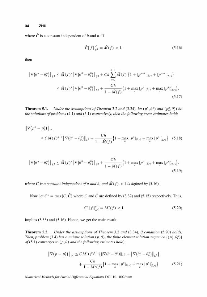
Theorem 5.1. Under the assumptions of Theorem 3.2 and (3.34), let (pn, θn) and (pnh, θn

h ) bethe solutions of problems (4.1) and (5.1) respectively, then the following error estimates hold:

∥∥∇(pn − pn

h

)∥∥Lr

≤ CM(f )n−1∥∥∇(

θ 0 − θ 0h

)∥∥L2 + Ch

1 − M(f )

{1 + max

n|pn|(2,r) + max

n|pn|r(2,r)

}(5.18)

∥∥∇(θn − θn

h

)∥∥L2 ≤ M(f )n

∥∥∇(θ 0 − θ 0

h

)∥∥L2 + Ch

1 − M(f )

{1 + max

n|pn|(2,r) + max

n|pn|r(2,r)

}.

(5.19)

where C is a constant independent of n and h, and M(f ) < 1 is defined by (5.16).

Now, let C∗ = max{C, C} where C and C are defined by (3.32) and (5.15) respectively. Thus,

C∗‖f ‖r ′Ld = M∗(f ) < 1 (5.20)

implies (3.33) and (5.16). Hence, we get the main result

Theorem 5.2. Under the assumptions of Theorem 3.2 and (3.34), if condition (5.20) holds.Then, problem (3.4) has a unique solution (p, θ), the finite element solution sequence {(pn

h, θnh )}

of (5.1) converges to (p, θ) and the following estimates hold,

∥∥∇(p − pn

h

)∥∥Lr ≤ CM∗(f )n−1

{‖∇(θ − θ 0)‖L2 + ∥∥∇(θ 0 − θ 0

h

)∥∥L2

}

+ Ch

1 − M∗(f )

{1 + max

n|pn|(2,r) + max

n|pn|r(2,r)

}(5.21)



∥∥∇(θ − θn

h

)∥∥L2 ≤ M∗(f )n

{‖∇(θ − θ 0)‖L2 + ∥∥∇(θ 0 − θ 0

h

)∥∥L2

}

+ Ch

1 − M∗(f )

{1 + max

n|pn|(2,r) + max

n|pn|r(2,r)

}. (5.22)

where C is a constant independent of n and h, and M∗(f ) < 1 is defined by (5.20).

Remark 5.3. We have to mention here that, (5.1.i) is still nonlinear problem which can be com-puted in practice by an iterative method such as, for example, augmented Lagrangian method [19]or conjugate gradient method [20].

References

1. J. Bass, Thermoelasticity, S.P. Parker, editor, McGraw-Hill encyclopedia of physics, McGraw-Hill,New York, 1982.

2. J. Baranger and A. Mikelic, Stationary solutions to a quasi-Newtonian flow with viscous heating, MathModels Methods Appl Sci 5 (1995), 725–738.

3. M. Boukrouche and G. Lukaszewicz, The stationary Stefan problem with convection governed by anon-linear Darcy’s law, Math Meth Appl Sci 22 (1999), 563–585.

4. U. Eisele, Introduction to polymer physics, Springer-Verlag, Berlin, 1990.

5. R. P. Gilbert and M. Fang, Nonlinear systems arising from nonisothermal, non-Newtonian Hele-Shawflows in the presence of body forces and sources, Math Comput Model 35 (2002), 1425–1444.

6. R. P. Gilbert and P. Shi, Nonisothermal, nonNewtonian Hele-Shaw flows. I. Mathematical formulation,in Proceeding on Transport Phenomenon, Technomic, Lancaster, 1992, pp. 1067–1088.

7. R. P. Gilbert and P. Shi, Nonisothermal, nonNewtonian Hele-Shaw flows. II. asymptotics and existenceof weak solutions, Nonlinear Anal 27 (1996), 539–559.

8. V. V. Zhikov, Meyers type estimates for the solution of a nonlinear Stokes system, Differential Equations33 (1997), 108–115.

9. J. Zhu, A. F. D. Loula, J. Karam, and J. N. C. Guerreiro, Finite element analysis of a coupled thermallydependent viscosity flow problem, Comput Appl Math 26 (2007), 45–66.

10. G. Cimatti, A bound for the temperature in the thermistor problem, IMA J Appl Math 40 (1988), 15–22.

11. G. Cimatti, Remarks on existence and uniqueness for the thermistor problem under mixed boundaryconditions, Q Appl Math 47 (1989), 117–121.

12. G. Cimatti and G. Prodi, Existence results for a nonlinear elliptic system modelling a temperaturedependent electrical resistor, Ann Mat Pura Appl 152 (1989), 227–236.

13. S. Clain, J. Rappaz, M. Swierkosz, and R. Touzani, Numerical modelling of induction heating fortwo-dimensional geometries, Math Models Methods Appl Sci 3 (1993), 805–822.

14. S. D. Howison, J. F. Rodrigues, and M. Shillor, Stationary solutions to the thermistor problem, J MathAnal Appl 174 (1993), 573–588.

15. T. Gallouët and R. Herbin, Existence of a solution to a coupled elliptic system, Appl Math Lett 7 (1994),49–55.

16. C. M. Elliott and S. Larsson, A finite element model for the time-dependent Joule heating problem,Math Comp 64 (1995), 1433–1453.

17. A. F. D. Loula and J. Zhu, Finite element analysis of a coupled nonlinear system, Comput Appl Math20 (2001), 321–339.

18. J. Zhu and A. F. D. Loula, Mixed finite element analysis of a thermally nonlinear coupled problem,Numer Methods Partial Differential Eq 22 (2006), 180–196.


36 ZHU

19. R. Glowinski and A. Marrocco, Sur l’approximation par éléments finis d’ordre un, et la résolution,par pénalisation-dualité, d’une classe de problèmes de Dirichlet non linéaires, RAIRO Anal Numér 2(1975), 41–76.

20. J. W. Barrett and W.-B. Liu, Finite element approximation of the p-Laplacian, Math Comp 61 (1993),523–537.

21. C. Ebmeyer and W.-B. Liu, Quasi-norm interpolation error estimates for the piecewise linear finiteelement approximation of p-Laplacian problems, Numer Math 100 (2005), 233–258.


Documents

Finite element analysis of thermally coupled nonlinear Darcy flows