Embed Size (px)
Citation preview
Int J Advanced Design and Manufacturing Technology, Vol. 11/ No. 1/ March - 2018 51
© 2018 IAU, Majlesi Branch
Finite Element Crushing
Analysis, Neural Network
Modelling and Multi-Objective
Optimization of the
Honeycomb Energy Absorbers Mahdi Vakili Department of Mechanical Engineering, College of Engineering,
University of Takestan, Takestan, Iran Email: [email protected]
Mohammad Reza Farahani * Department of Mechanical Engineering, College of Engineering,
University of Tehran, Tehran, Iran
Email: [email protected]
*Corresponding author
Abolfazl Khalkhali Department of Automotive Engineering, Iran University of Science and
Technology, Tehran, Iran
Email: [email protected]
Received: 18 September 2017, Revised: 21 October 2017, Accepted: 28 November 2017
Abstract: The thin-walled honeycomb structures are one of the most common energy absorber types. These structures are of particular use in different industries due to their high energy absorption capability. In this article, the finite element simulation of honeycomb energy absorbers was accomplished in order to analyze their crushing behavior. 48 panels with different hexagonal edge length, thickness and branch angle were examined. In the following, the amounts of mean stresses versus the geometric variables using neurotic lattices were considered. Comparison between the finite element results and the obtained neural network model verified the high accuracy of the obtained model. Then the model was optimized by one of the efficient genetic algorithm methods called “Multi-objective Uniform-diversity Genetic algorithm”. The obtained optimum results provide practical information for the design and application of these energy absorbers regards to designer requirement. It was observed that honeycomb energy absorbers with 11.07 mm hexagonal edge length, 0.078 mm wall thickness and 123-degree branch angle have the maximum energy absorption over the panel mass.
Keywords: Energy absorbers, Honeycomb, Multi-Objective optimization, Neural-Network modeling
Reference: Mahdi Vakili, Mohammad Reza Farahani, and Abolfazl Khalkhali, “Finite Element Crushing Analysis, Neural Network Modelling and Multi-Objective Optimization of the Honeycomb Energy Absorbers”, Int J of Advanced Design and Manufacturing Technology, Vol. 11/No. 1, 2018, pp. 51-59.
Biographical notes: M. Vakili is a MSc of Mechanical Engineering at University of Takestan. His current research interest mainly focuses on finite element modelling, and thin wall structures. M. Farahani is associate professor of mechanical engineering at the University of Tehran, Iran. His current research focuses on numerical and experimental modelling. A. Khalkhali is assistant professor of automotive engineering department, Iran University of Science and Technology. His current research focuses on multi objective optimization.
52 Int J Advanced Design and Manufacturing Technology, Vol. 11/ No. 1/ March - 2018
© 2018 IAU, Majlesi Branch
1 INTRODUCTION
Along with advances in technology, the power and the
speed of moving components were increased which raise
the risk of adverse events with releasing a high amount
of energy in these systems. For example, the energy
release of a boiler, a nuclear power plant or likelihood of
bopping the vehicles. Thus, in recent years, the design of
the structures with the capability of controlling the
unwanted freed energy was considered. Thin-walled
structures are one of the energy absorbers that have
found wide application. This type of structure can
tolerate large plastic deformation under the applied load
and so absorb a high amount of energy. Plastic behavior
of elements such as thin-walled tubes, thin-walled cans
and spherical shells have been investigated during last
four decades. [1]- [7].
Weirzbiki [8] for the first time presented a new method
that provides an analytical model for describing the
behavior of honeycomb structures under compressive
static loads. The thin-walled honeycomb structures have
very extended application due to their good energy
absorbing capability. Several researchers were
investigating the behavior of this type of energy
absorbers under different dynamic and static loads, using
experimental, numerical and analytical methods. [9]-
[12].
In this research, modeling of the energy absorption
capacity of the honeycomb energy absorbers versus the
panel mass was considered. Wide ranges of geometrical
parameters were studied in order to optimize the panel
geometries using multi-objective optimization
technique.
2 FINITE ELEMENT MODELING OF THE
HONEYCOMB STRUCTURE CRUSHING
In this section, crushing of the honeycomb structures
was analyzed using commercial software,
ABAQUS/Explicit. Cell specification of the honeycomb
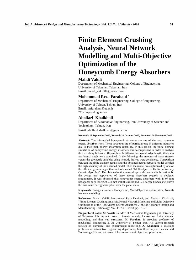
panel was depicted in Fig. 1, where d is each hexagonal
edge length, t is the wall thickness, α is the branch angle
and l is the length of the honeycomb which 100 mm is
considered in this study.
Fig. 1 Initial model of the honeycomb energy absorber
One specific cell as depicted in Fig. 1 has a “Y” shape
cross section, where consists of two single walls and one
double wall.
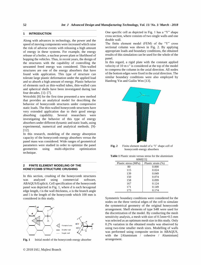
The finite element model (FEM) of the “Y” cross
sectional column was shown in Fig. 2. By applying
appropriate loads and boundary conditions, the obtained
results of this simulation can be used for the whole of the
panel.
In this regard, a rigid plate with the constant applied
velocity of 10 m s-1 is considered at the top of the model
to compress the column in the axial direction. All nodes
of the bottom edges were fixed in the axial direction. The
similar boundary conditions were also employed by
Hanfeng Yin and Guilin Wen [13].
Fig. 2 Finite element model of a ‘Y’ shape cell of
honeycomb energy absorbers
Table 1 Plastic strain versus stress for the aluminium
6060[15]
Plastic stress (MPa) Plastic strain (%)
80
115
139
150
158
167
171
173
0.000
0.024
0.049
0.074
0.099
0.124
0.149
0.174
Symmetric boundary conditions were considered for the
nodes on the three vertical edges of the cell to simulate
the symmetrical geometry of the original honeycomb
arrangement. Shell elements of type S4R were used for
the discretization of the model. By conducting the mesh
sensitivity analysis, a mesh with size of 0.5mm×0.5 mm
was selected as an optimum mesh size in this study. Only
0.2% variation in the obtained results was observed by
using two-time smaller mesh sizes. Modelling of walls
was performed using composite section in ABAQUS,
with the [Aluminium / cohesive / Aluminium]
arrangement.
Int J Advanced Design and Manufacturing Technology, Vol. 11/ No. 1/ March - 2018 53
© 2018 IAU, Majlesi Branch
The employed material was the AA6060-T4 aluminium
alloy with physical properties of density ρ = 2.7 (10−3)
gr*mm-3, Young’s modulus E = 68.2 GPa. The plastic
behaviour of the aluminium was considered according to
the stress-strain data presented in Table 1. The elastic
modulus of the adhesive has been considered E = 5 GPa
with the ultimate strength σu = 40 MPa [14]. In the
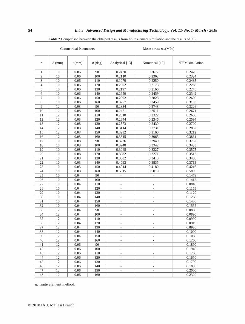
present study, 48 different models were simulated and
mean crushing stress (σm) was calculated for each model.
Mean crushing stress (σm) was obtained using the
following Eq. (1).
𝜎𝑚 = (∫ 𝜎(𝜀) 𝑑𝜀𝜀
0)/𝜀 (1)
Where σ(ε) and ε are the axial crushing stress and strain
respectively. The dimensions and the obtained results for
half of the models were presented in Table 2. The
obtained results were compared with the results of [13].
In order to quantify the differences between these
results, the error parameters R2, RMSE and MAPE were
used from Eqs. (2)-(4).
𝑅2 = 1 − (∑ (𝑇𝑗 − 𝑂𝑗)2
𝑗 ) /(∑ (𝑂𝑗)2
𝑗 ) (2)
𝑅𝑀𝑆𝐸 = (1
𝑃 ∑ |𝑇𝑗 − 𝑂𝑗 |
2𝑗 )
1
2 (3)
𝑀𝐴𝑃𝐸 = 1
𝑃 ∑ (|(𝑇𝑗 − 𝑂𝑗)/𝑇𝑗|) 100 𝑗 (4)
Where T is the results of [13] O is the obtained value and
P is the number of samples.
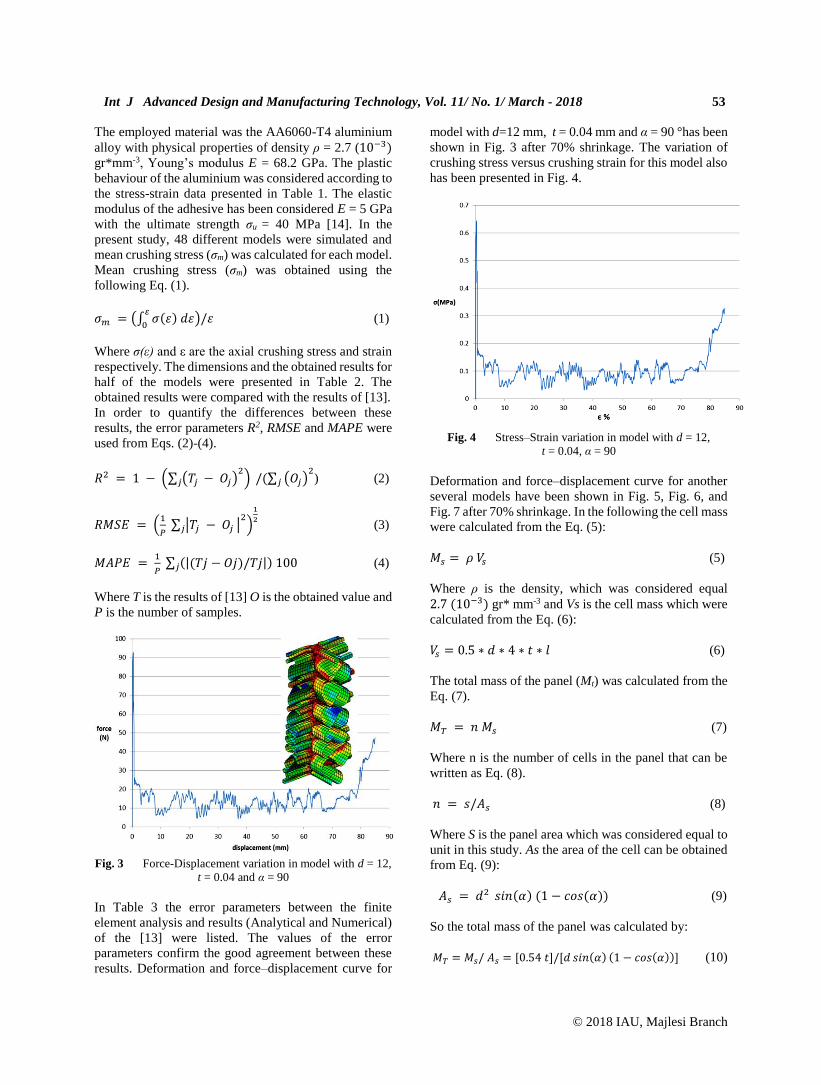
Fig. 3 Force-Displacement variation in model with d = 12,
t = 0.04 and α = 90
In Table 3 the error parameters between the finite
element analysis and results (Analytical and Numerical)
of the [13] were listed. The values of the error
parameters confirm the good agreement between these
results. Deformation and force–displacement curve for
model with d=12 mm, t = 0.04 mm and α = 90 °has been
shown in Fig. 3 after 70% shrinkage. The variation of
crushing stress versus crushing strain for this model also
has been presented in Fig. 4.
Fig. 4 Stress–Strain variation in model with d = 12,
t = 0.04, α = 90
Deformation and force–displacement curve for another
several models have been shown in Fig. 5, Fig. 6, and
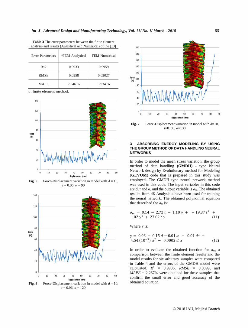
Fig. 7 after 70% shrinkage. In the following the cell mass
were calculated from the Eq. (5):
𝑀𝑠 = 𝜌 𝑉𝑠 (5)
Where ρ is the density, which was considered equal
2.7 (10−3) gr* mm-3 and Vs is the cell mass which were
calculated from the Eq. (6):
𝑉𝑠 = 0.5 ∗ 𝑑 ∗ 4 ∗ 𝑡 ∗ 𝑙 (6)
The total mass of the panel (Mt) was calculated from the
Eq. (7).
𝑀𝑇 = 𝑛 𝑀𝑠 (7)
Where n is the number of cells in the panel that can be
written as Eq. (8).
𝑛 = 𝑠/𝐴𝑠 (8)
Where S is the panel area which was considered equal to
unit in this study. As the area of the cell can be obtained
from Eq. (9):
𝐴𝑠 = 𝑑2 𝑠𝑖𝑛(𝛼) (1 − 𝑐𝑜𝑠(𝛼)) (9)
So the total mass of the panel was calculated by:
𝑀𝑇 = 𝑀𝑠/ 𝐴𝑠 = [0.54 𝑡]/[𝑑 𝑠𝑖𝑛(𝛼) (1 − 𝑐𝑜𝑠(𝛼))] (10)
54 Int J Advanced Design and Manufacturing Technology, Vol. 11/ No. 1/ March - 2018
© 2018 IAU, Majlesi Branch
Table 2 Comparison between the obtained results from finite element simulation and the results of [13]
Geometrical Parameters Mean stress σm (MPa)
n d (mm) t (mm) α (deg) Analytical [13] Numerical [13] aFEM simulation
1 10 0.06 90 0.2420 0.2677 0.2470
2 10 0.06 100 0.2110 0.2362 0.2334
3 10 0.06 110 0.1979 0.2250 0.2435
4 10 0.06 120 0.2002 0.2173 0.2258
5 10 0.06 130 0.2197 0.2166 0.2245
6 10 0.06 140 0.2659 0.2459 0.2349
7 10 0.06 150 0.2802 0.2828 0.2600
8 10 0.06 160 0.3257 0.3459 0.3103
9 12 0.08 90 0.2834 0.2748 0.3226
10 12 0.08 100 0.2471 0.2511 0.2671
11 12 0.08 110 0.2318 0.2322 0.2658
12 12 0.08 120 0.2344 0.2346 0.2594
13 12 0.08 130 0.2573 0.2439 0.2700
14 12 0.08 140 0.3114 0.2731 0.2852
15 12 0.08 150 0.3282 0.3160 0.3212
16 12 0.08 160 0.3815 0.3965 0.3861
17 10 0.08 90 0.3726 0.3940 0.3752
18 10 0.08 100 0.3248 0.3342 0.3433
19 10 0.08 110 0.3048 0.3327 0.3575
20 10 0.08 120 0.3082 0.3271 0.3512
21 10 0.08 130 0.3382 0.3413 0.3408
22 10 0.08 140 0.4093 0.3835 0.3713
23 10 0.08 150 0.4314 0.4180 0.4216
24 10 0.08 160 0.5015 0.5019 0.5009
25 10 0.04 90 - - 0.1478
26 10 0.04 100 - - 0.1412
27 10 0.04 110 - - 0.0840
28 10 0.04 120 - - 0.1153
29 10 0.04 130 - - 0.1120
30 10 0.04 140 - - 0.1268
31 10 0.04 150 - - 0.1430
32 10 0.04 160 - - 0.1555
33 12 0.04 90 - - 0.0860
34 12 0.04 100 - - 0.0890
35 12 0.04 110 - - 0.0990
36 12 0.04 120 - - 0.0919
37 12 0.04 130 - - 0.0920
38 12 0.04 140 - - 0.1000
39 12 0.04 150 - - 0.1060
40 12 0.04 160 - - 0.1260
41 12 0.06 90 - - 0.1890
42 12 0.06 100 - - 0.1940
43 12 0.06 110 - - 0.1760
44 12 0.06 120 - - 0.1650
45 12 0.06 130 - - 0.1790
46 12 0.06 140 - - 0.1890
47 12 0.06 150 - - 0.2000
48 12 0.06 160 - - 0.2320
a: finite element method.
Int J Advanced Design and Manufacturing Technology, Vol. 11/ No. 1/ March - 2018 55
© 2018 IAU, Majlesi Branch
Table 3 The error parameters between the finite element
analysis and results (Analytical and Numerical) of the [13]
Error Parameters aFEM-Analytical FEM-Numerical
R^2 0.9933 0.9959
RMSE 0.0258 0.02027
MAPE 7.846 % 5.934 %
a: finite element method.
Fig. 5 Force-Displacement variation in model with d = 10,
t = 0.06, α = 90
Fig. 6 Force-Displacement variation in model with d = 10,
t = 0.06, α = 120
Fig. 7 Force-Displacement variation in model with d=10,
t=0. 08, α=130
3 ABSORBING ENERGY MODELING BY USING
THE GROUP METHOD OF DATA HANDLING NEURAL
NETWORKS
In order to model the mean stress variation, the group
method of data handling (GMDH) - type Neural
Network design by Evolutionary method for Modeling
(GEVOM) code that is prepared in this study was
employed. The GMDH–type neural network method
was used in this code. The input variables in this code
are d, t and α, and the output variable is σm. The obtained
results from 48 Analysis’s have been used for training
the neural network. The obtained polynomial equation
that described the σm is:
𝜎𝑚 = 0.14 − 2.72 𝑡 − 1.10 𝑦 + + 19.37 𝑡2 + 1.02 𝑦2 + 27.02 𝑡 𝑦 (11)
Where y is:
𝑦 = 0.03 + 0.15 𝑑 − 0.01 𝛼 − 0.01 𝑑2 + 4.54 (10−5) 𝛼2 − 0.0002 𝑑 𝛼 (12)
In order to evaluate the obtained function for σm, a
comparison between the finite element results and the
model results for six arbitrary samples were compared
in Table 4 and the errors of the GMDH model were
calculated. R2 = 0.9986, RMSE = 0.0099, and
MAPE = 2.267% were obtained for these samples that
confirm the small error and good accuracy of the
obtained equation.
56 Int J Advanced Design and Manufacturing Technology, Vol. 11/ No. 1/ March - 2018
© 2018 IAU, Majlesi Branch
Table 4 Comparison between obtained σm from GEVOM
model and ABAQUS results for six arbitrary samples
Geometrical Parameters Mean stress σm (MPa)
d (mm) t (mm) α (deg) Gevom aFEM
10 0.07 155 0.2807 0.3600
11 0.08 115 0.3090 0.3089
11 0.05 115 0.1492 0.1480
10.5 0.06 125 0.2130 0.2104
12 0.07 135 0.2258 0.2250
10 0.07 105 0.2807 0.3023
a: finite element method.
4 MULTI-OBJECTIVE OPTIMIZATION OF
HONEYCOMB ENERGY ABSORBER
In this section multi-objective optimization method
using Multi-Objective Uniform-diversity Genetic
Algorithms (MUGA) was employed for two different
cases. For the first case, σm maximizing and Ms / As minimizing and for the second case, maximizing the σm
and As and minimizing the 𝑀𝑠 were considered.
For each case, the optimal points were found and the
Pareto chart was presented.
Upper and lower limits for the input variables are these
Eqs. (13) - (15).
10𝑚𝑚 ≤ 𝑑 ≤ 12𝑚𝑚 (13)
0.04𝑚𝑚 ≤ 𝑡 ≤ 0.08𝑚𝑚 (14)
90° ≤ 𝛼 ≤ 160° (15)
4.1. The first case optimization
In this case 𝜎𝑚 And Ms / As have been the objective
functions. The first objective function 𝜎𝑚 should be
maximized and the second objective function Ms / As
should be minimized. Since this optimization was based
on minimization, the first objective function was
reversed (1 / 𝜎𝑚) and minimized. After the optimization,
the Pareto points of the objective functions were plotted
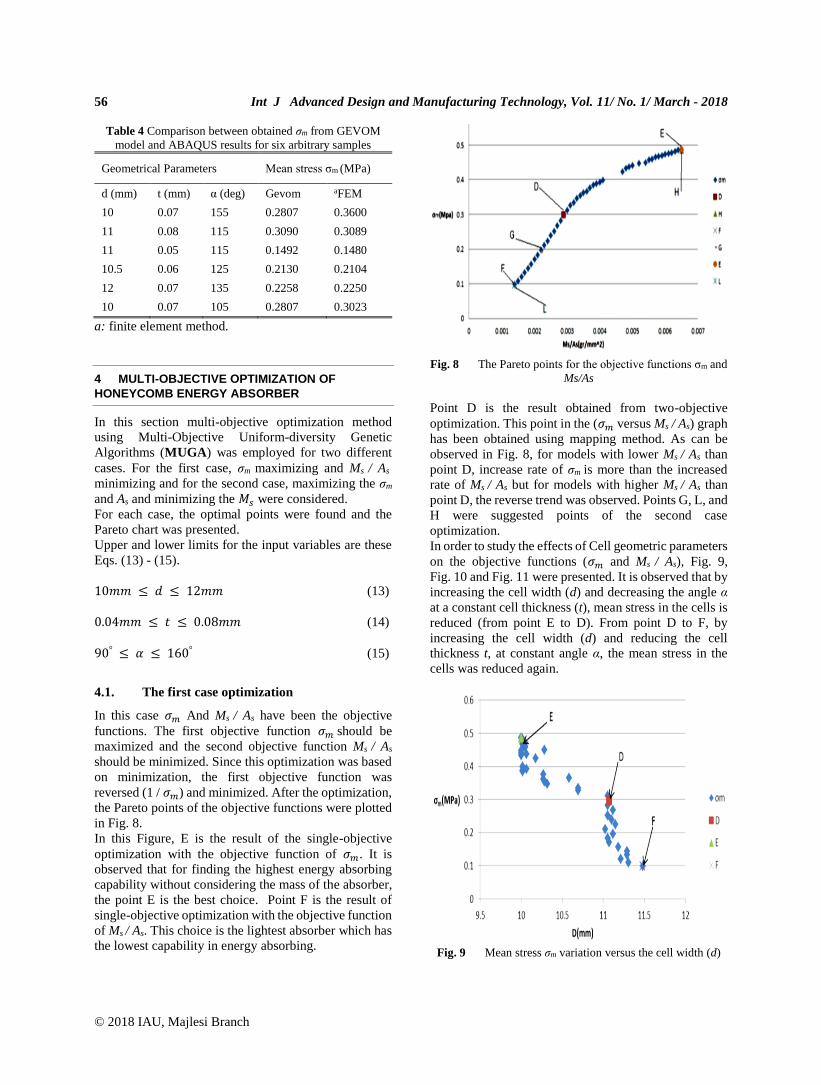
in Fig. 8.
In this Figure, E is the result of the single-objective
optimization with the objective function of 𝜎𝑚. It is
observed that for finding the highest energy absorbing
capability without considering the mass of the absorber,
the point E is the best choice. Point F is the result of
single-objective optimization with the objective function
of Ms / As. This choice is the lightest absorber which has
the lowest capability in energy absorbing.
Fig. 8 The Pareto points for the objective functions σm and
Ms/As
Point D is the result obtained from two-objective
optimization. This point in the (𝜎𝑚 versus Ms / As) graph
has been obtained using mapping method. As can be
observed in Fig. 8, for models with lower Ms / As than
point D, increase rate of σm is more than the increased
rate of Ms / As but for models with higher Ms / As than
point D, the reverse trend was observed. Points G, L, and
H were suggested points of the second case
optimization.
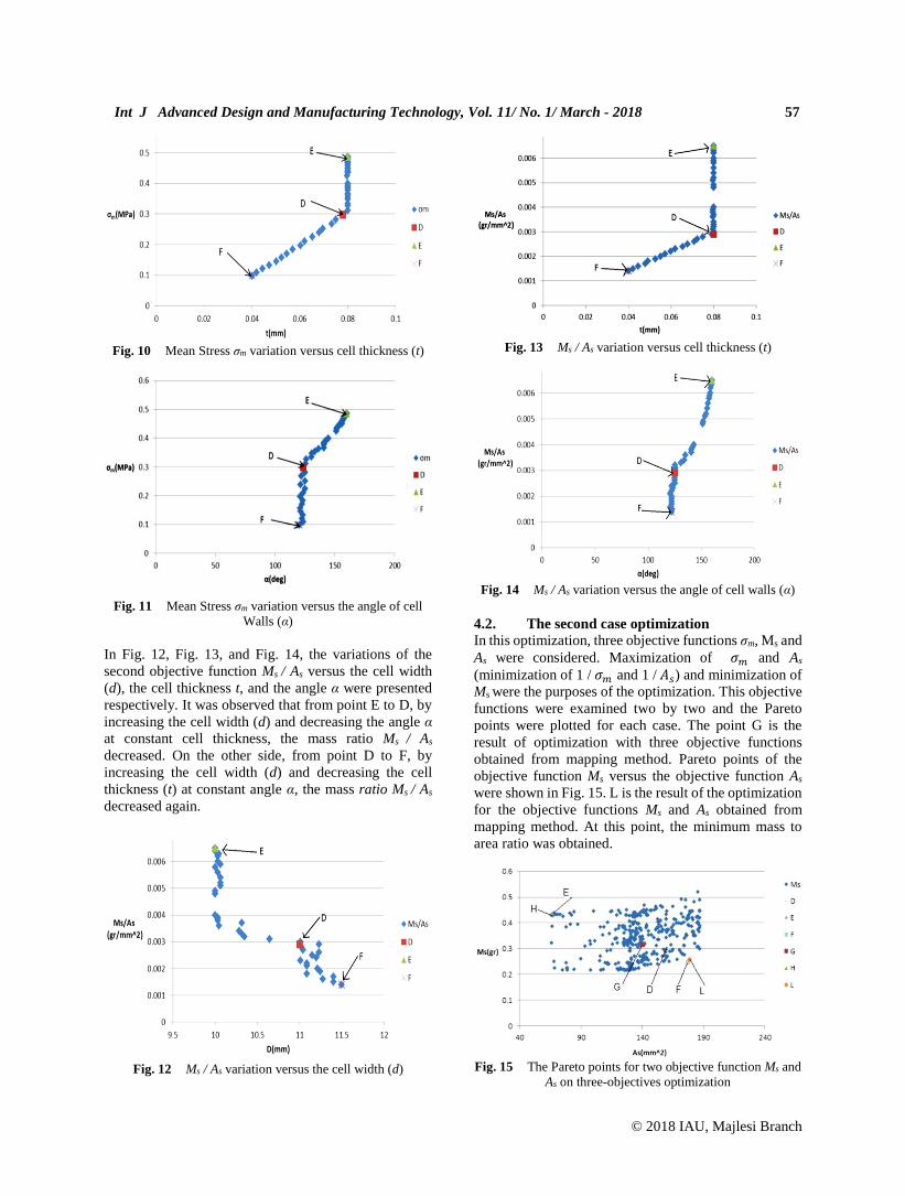
In order to study the effects of Cell geometric parameters
on the objective functions (𝜎𝑚 and Ms / As), Fig. 9,
Fig. 10 and Fig. 11 were presented. It is observed that by
increasing the cell width (d) and decreasing the angle α
at a constant cell thickness (t), mean stress in the cells is
reduced (from point E to D). From point D to F, by
increasing the cell width (d) and reducing the cell
thickness t, at constant angle α, the mean stress in the
cells was reduced again.
Fig. 9 Mean stress σm variation versus the cell width (d)
Int J Advanced Design and Manufacturing Technology, Vol. 11/ No. 1/ March - 2018 57
© 2018 IAU, Majlesi Branch
Fig. 10 Mean Stress σm variation versus cell thickness (t)
Fig. 11 Mean Stress σm variation versus the angle of cell
Walls (α)
In Fig. 12, Fig. 13, and Fig. 14, the variations of the
second objective function Ms / As versus the cell width
(d), the cell thickness t, and the angle α were presented
respectively. It was observed that from point E to D, by
increasing the cell width (d) and decreasing the angle α
at constant cell thickness, the mass ratio Ms / As
decreased. On the other side, from point D to F, by
increasing the cell width (d) and decreasing the cell
thickness (t) at constant angle α, the mass ratio Ms / As
decreased again.
Fig. 12 Ms / As variation versus the cell width (d)
Fig. 13 Ms / As variation versus cell thickness (t)
Fig. 14 Ms / As variation versus the angle of cell walls (α)
4.2. The second case optimization
In this optimization, three objective functions σm, Ms and
As were considered. Maximization of 𝜎𝑚 and As
(minimization of 1 / 𝜎𝑚 and 1 / 𝐴𝑠) and minimization of
Ms were the purposes of the optimization. This objective
functions were examined two by two and the Pareto
points were plotted for each case. The point G is the
result of optimization with three objective functions
obtained from mapping method. Pareto points of the
objective function Ms versus the objective function As
were shown in Fig. 15. L is the result of the optimization
for the objective functions Ms and As obtained from
mapping method. At this point, the minimum mass to
area ratio was obtained.
Fig. 15 The Pareto points for two objective function Ms and
As on three-objectives optimization
58 Int J Advanced Design and Manufacturing Technology, Vol. 11/ No. 1/ March - 2018
© 2018 IAU, Majlesi Branch
Fig. 16 The Pareto points for two objective function σm and
As on three-objective optimization
Pareto points of the objective functions σm versus As and
σm versus Ms were presented in Fig. 16 and Fig. 17,
respectively. It was shown in Fig. 16 that point H have
the maximum σm and consequently the maximum energy
absorbing capability. Points E and H were the optimum
results from two and three-objective optimizations
respectively. As observed in Fig. 17, these points had the
largest σm between the other obtained points and were
close to each other. On the other side, it was observed
that points L and F that had the minimum Ms/As ratio
were also close to each other. So it can be concluded that
the results of two and three objective optimizations are
similar.
Fig. 17 The Pareto points for two objective functions σm
and Ms on three objective optimization
Table 5 Energy absorber geometrical parameters proposed from optimization
Offer
points
d (mm) t (mm) α (deg) As (mm2) Ms (gr) Ms/As (gr*mm-2) σm (MPa)
D 11.07 0.078 123.62 160.70 0.4660 0.0029 0.2979
E 10.00 0.080 160.00 66.46 0.4320 0.0065 0.4866
F 11.48 0.040 120.32 177.12 0.2480 0.0014 0.0983
G 10.45 0.055 125.8 140.50 0.3148 0.0022 0.1912
H 10.00 0.080 160.00 66.34 0.4320 0.0065 0.4866
L 11.78 0.040 125.27 178.70 0.2564 0.0014 0.0963
5 CONCLUSION
The finite element simulation of honeycomb energy
absorbers was accomplished under axial pressure load in
order to analyze their crushing behavior. The obtained
results were verified by comparison with the results from
ref [13]. The very small error values represented the high
performance of the developed finite element model. In
the following, a respect is getting for the amount of mean
crushing stress versus the geometric variables using
neurotic lattices. By using the GEVOM code, a
functional model which describes the mean stress (σm) in
terms of the cell width (d), wall thickness (t), and the cell
angle (α) was obtained. The performance of the model
was examined in six randomly selected samples. The σm
values obtained from this model were compared with the
results of the finite element simulation. Small error
parameters between the model results and the calculated
finite element results proved the high accuracy of the
obtained function. Multi-objective optimization
technique was employed in order to optimize the
honeycomb energy absorbers. The Pareto points were
obtained in all the studied cases. For the first case, σm
maximize and Ms/As minimize and for the second case,
maximizing the σm and As and minimizing the Ms were
considered. Two and three-objective optimizations were
carried out which indicated that the two and three-
objective optimization results are similar. The obtained
optimum results provide practical information for the
design and application of these energy absorbers regards
to designer requirement.
ACKNOWLEDGMENTS
I would like to express my special gratitude and thanks
to Dr. Jamali for giving valuable guidance and kind
assistance.
Int J Advanced Design and Manufacturing Technology, Vol. 11/ No. 1/ March - 2018 59
© 2018 IAU, Majlesi Branch
REFERENCES
[1] Alexander, J. M., “An Approximate Analysis of the Collapse of Thin Cylindrical Shells Under Axial Loadingˮ, Q J. Mechanics Appl Math, Vol. 13, 1960, pp. 10-15.
[2] Johnson, W., Mamalis, A. G., “Crashworthiness of Vehicles Londonˮ, Mech. Eng Publications Ltd. London, 1978.
[3] Johnson, W., Reid, S. R., “Metallic Energy Dissipating Systemsˮ, ASME Applied Mechanics Review, Vol. 31, 1978, pp. 277-288.
[4] Jones, N., Wierzbicki, T., “Structural Crashworthinessˮ, Butterworth and Co Publishers, London, 1983.
[5] Mamalis, A. G., Johnson, W., “The Quasi-Static Crumpling of Thin Walled Circular Cylinders and Frusta Under Axial Compressionˮ, Int J Mech Sci, Vol. 25, 1983, pp. 713-732.
[6] Abramowicz, W., Jones, N., “Dynamic Axial Crushing of Square Tubeˮ, Int J of Impact Eng, Vol. 2, 1984, pp. 179-208.
[7] Jones, N., Abramowicz, W., “Static and Dynamic Axial Crushing of Circular and Square Tubes. Proceeding of the Symposium on Metal Forming and Impact Mechanicsˮ, Oxford: Pergamon Press, 1985.
[8] Wierzbicki, T., “Crushing Analysis of Metal Honeycombˮ, Int. J. Impact Eng., Vol. 1, 1983, pp. 157-174.
[9] Zhang, J., Ashby, M. F., “The Out of Plane Properties of Honeycombˮ, Int. J. Mech Sci, Vol. 34, 1992, pp. 475-489.
[10] Shahmirzaloo, A., Farahani, M., “Determination of Local Constitutive Properties of Aluminium Using Digital Image Correlation: A Comparative Study Between Uniform Stress and Virtual Fieldsˮ, Int J of Advanced Design and Manufacturing Technology, Under publication.
[11] Sam Daliri, O., Farahani, M., “Characterization of Stress Concentration in Thin Cylindrical Shells with Rectangular Cutoutˮ, Int J of Advanced Design and Manufacturing Technology, Vol. 2, No. 1, 2008, pp. 43–54.
[12] Alavi Nia, A., Sadeghi, M. Z., “The Effects of Foam Filling on Compressive Response of Hexagonal Cell Aluminum Honeycombs Under Axial Loading. Experimental Studyˮ, Mater des., Vol. 31, 2010, pp. 1216–1230.
[13] Yin, H., Wen, G., “Theoretical Prediction and Numerical Simulation of Honeycomb Structures with Various Cell Specifications Under Axial Loadingˮ, Int. J. Mech Mater Des., Vol. 7, 2011, pp. 253–263.
[14] Higgins, A., “Adhesive Bonding of Aircraft Structuresˮ, Int. J. Adhes., Vol. 20, 2000, pp. 367–376.
[15] Santosa, S. P., Wierzbicki, T., Hanssen, A. G., “Experiment and Numerical Studies of Foam-Filled Sectionsˮ, Int. J. Impact Eng., Vol. 24, 2000, pp. 509–534.