FINITE ELEMENT METHODS FOR ELLIPTIC PROBLEMSneela/CIMPA/notes/AmiyaPani.pdf · FINITE ELEMENT METHODS FOR ELLIPTIC PROBLEMS 1 ... (FEM) ... I have never intended to write a Lecture

Lecture Notes

On

FINITE ELEMENT METHODS FOR

ELLIPTIC PROBLEMS1

Amiya Kumar Pani

Industrial Mathematics GroupDepartment of Mathematics

Indian Institute of Technology, BombayPowai, Mumbai-4000 76 (India).

IIT Bombay, March 2012 .

1Workshop on ‘Mathematical Foundation of Advanced Finite Element Methods(MFAFEM-2013) held in BITS,GOA during 26th December - 3rd January, 2014

‘ Everything should be made simple, but not simpler’.

- Albert Einstein.

Contents

Preface I

1 Introduction 11.1 Background. . . . . . . . . . . . . . . . . . . . . . . . . . . . . . 11.2 Finite Difference Methods (FDM). . . . . . . . . . . . . . . . . . 41.3 Finite Element Methods (FEM). . . . . . . . . . . . . . . . . . . 8

2 Theory of Distribution and Sobolev Spaces 102.1 Review of L2- Space. . . . . . . . . . . . . . . . . . . . . . . . . 102.2 A Quick Tour to the Theory of Distributions. . . . . . . . . . . . 132.3 Elements of Sobolev Spaces . . . . . . . . . . . . . . . . . . . . . 19

3 Abstract Elliptic Theory 283.1 Abstract Variational Formulation . . . . . . . . . . . . . . . . . . 293.2 Some Examples. . . . . . . . . . . . . . . . . . . . . . . . . . . . 33

4 Elliptic Equations 474.1 Finite Dimensional Approximation to the Abstract Variational

Problems. . . . . . . . . . . . . . . . . . . . . . . . . . . . . . . . 474.2 Examples. . . . . . . . . . . . . . . . . . . . . . . . . . . . . . . . 504.3 Computational Issues . . . . . . . . . . . . . . . . . . . . . . . . 584.4 Adaptive Methods. . . . . . . . . . . . . . . . . . . . . . . . . . 62

Bibliography 67

I

HOW THESE NOTES CAME TO BE

I have never intended to write a Lecture Note on this topic, as there are manyexcellent books available in literature. But, when a group of enthusiastic facultymembers in the Department of Mathematics at the Universidade Federale doParana (UFPR) requested me to give some lectures on the theory of finiteelements, I immediately rushed to the Central Library of UFPR to check somebooks on this topic. To my dismay (may be it is a boon in disguise), I couldnot find any relevant books in the library here. More over, in my first lecture, Irealised the urgent need of supplying some notes in order to keep their intereston. However, thank to Professor Vidar Thomee, I had his notes entitled Lectureson Approximation of Parabolic Problems by Finite Elements [13] and thank tothe netscape for downloading [7] from the home page of Professor D. Estep fromCALTEC. So in an attempt to explain the lectures given by Professor Vidar atIIT, Bombay , first four chapters are written. Thank to LATEX and Adriana,she typed first chapter promptly and then the flow was on. So by the end ofthe series, we had these notes. At this point let me point out that the writeup is influenced by the style of Mercier [10] (although the book is not availablehere, but it is more due to my experience of using this book for a course at IIT,Bombay).

Sometimes back, I asked myself: Is there any novelty in the present ap-proach? Well, (Bem!) the answer is certainly in negative. But for the followingsimple reason this one may differ from those books written by stalwarts of thisfield : Some questions are posed in the introductory chapter and throughout thisseries, attempts have been made to provide some answers. Moreover for finiteelement methods, the usefulness of Lax equivalence theorem has been high-lighted throughout these notes and the role as well as the appropriate choiceof intermediate or auxiliary projection has been brought out in the context offinite element approximations to parabolic problems.

It seems to be a standard practice that in the Preface the author should givea brief description of each chapter of his / her book. In order to pay respectto our tradition, I (although first person is hardly used in writing articles) ammaking an effort to present some rudiments of each chapter of this lecture note.

In the introductory chapter, some basic (!) questions are raised and in thesubsequent chapters, some answers have been provided. To motivate the finite

element methods, a quick description on the finite difference method to thePoisson’s equation is also given.

Chapter 2 is devoted to a quick review of the theory of distribution, gener-alised derivatives and some basic elements of Sobolev spaces. Concept of traceand Poincare inequality are also discussed in this chapter.

In chapter 3, a brief outline of abstract variational theory is presented .A proof of Lax-Milgram Theorem is also included. Several examples on ellipticproblems are discussed and the question of solvability of their weak formulationsare examined.

Chapter 4 begins with a brief note on the finite dimensional approximationto the abstract variational problems. An introduction of finite element methodsapplied to two elliptic problems is also included. A priori error estimates arealso derived. Based on Eriksson et al. [7], an adaptive procedure is outlinedwith a posteriori error estimates.

I am indebted to Professors Bob Anderssen, Purna C. Das, Ian Sloan,Graeme Fairweather, Vidar Thomee and Lars Wahlbin for introducing me thebeautiful facets of Numerical Analysis. The present set of notes is a part ofthe lectures given in the Department of Mathematics at Federal University ofParana, Curitiba. This would have not been possible without the support ofProfessor Jin Yun Yuan. He helped me in typing and correcting the manuscript.He is a good human being and a good host and I shall recommend the readers tovisit him. I greately acknowledge the financial support provided by the UFPR.Thank to the GOROROBA group for entertaining me during lunch time and Ialso acknowledge the moral support provided by the evening cafe club members(Carlos, Correa Eidem, Fernando (he is known for his improved GOROROBA),Jose, Zeca). Perhapse, it would be incomplete if I do not acknowledge the sup-port and encouragement given by my wife Tapaswini. She allowed me to comehere in a crucial juncture of her life. Thanks to the email facility through whichI get emails from my son Aurosmit and come to know more about my new bornbaby ‘ Anupam’ ( I am waiting eagerly to see him, he was born when I wasaway to Curitiba). I would like to express my heart felt thank to the familyof Professor Jin Yun and Professor Beatriz for showing me some nice places inand around Curitiba. Finally, I am greately indebted to my friend ProfessorKannan Moudgalya and his family for their help and moral support providedto my family during my abscence.

Amiya Kumar Pani

Chapter 1

Introduction

In this introductory chapter, we briefly describe various issues related tofinite element methods for solving differential equations.

1.1 Background.

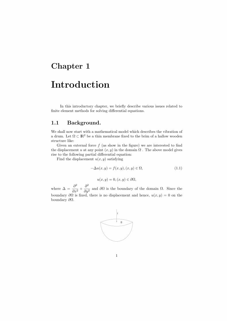
We shall now start with a mathematical model which describes the vibration ofa drum. Let Ω ⊂ IR2 be a thin membrane fixed to the brim of a hallow woodenstructure like:

Given an external force f (as show in the figure) we are interested to findthe displacement u at any point (x, y) in the domain Ω . The above model givesrise to the following partial differential equation:

Find the displacement u(x, y) satisfying

−∆u(x, y) = f(x, y), (x, y) ∈ Ω, (1.1)

u(x, y) = 0, (x, y) ∈ ∂Ω,

where ∆ =∂2

∂x2+

∂2

∂y2and ∂Ω is the boundary of the domain Ω. Since the

boundary ∂Ω is fixed, there is no displacement and hence, u(x, y) = 0 on theboundary ∂Ω.

f

Ω

1

CHAPTER 1. INTRODUCTION 2

a

uo

x

By a solution (classical ) u of (1.1), we mean a twice continuously differen-tiable function u which satisfies the partial differential equation (1.1) at eachpoint (x, y) in Ω and also the boundary condition. Note that f has to be con-tinuous, if we are looking for the classical solutions of (1.1). For the presentproblem, the external force f may not be imparted continuously. In fact f canbe a point force, i.e., a force applied at a point in the domain. Thus a physicallymore relevant problem is to allow more general f , that is, f may have some dis-countinuities. Therefore, there is a need to generalize the concept of solutions.In early 1930, S.L. Sobolev came across with a similar situation while he wasdealing with the following first order hyperbolic equation:

ut + aux = 0, t > 0, −∞ < x <∞u(x, 0) = u0(x), −∞ < x <∞. (1.2)

Here, a is a real, positive constant and u0 is the initial profile. It is well knowthe exact solution u(x, t) = u0(x− at). In this case, the solution preserves theshape of the initial profile. However, if u0 is not differentiable (say it has a kink)the solution u is stillmeaningful physically, but not in the sense of classical solution. These observa-tions were instrumental for the development of the modern partial differentialequations.

Again comming back to our vibration of drum problem, we note that inmechanics or in physics, the same model is described through a minimizationof total energy, say J(v), i.e., minimization of J(v) subjects to the set V of allpossible admissible displacements, where

J(v) =1

2

∫Ω

(|∂v∂x

|2 + |∂v∂y

|2) dxdy︸︷︷︸Kinetic Energy mass being unit

−∫Ω

fv dxdy︸︷︷︸Potential Energy

(1.3)

and V is a set of all possible displacements v such that the above integrals aremeaningful and v = 0 on ∂Ω. More precisely, we cast the above problem asFind u ∈ V such that u = 0 on ∂Ω and u minimize J , that is,

J(u) =Minv∈V

J(v). (1.4)


The advantage of the second formulation is that the displacement u maybe once continuously differentiable and the external force f may be of generalform, i.e., f may be square integrable and may allow discontinuties. Further,it is observed that every solution u of (1.1) satisfies (1.4) (it is really not quiteaparrent, but it is indeed possible, this point we shall closely examine later onin the course of my lectures). However, the converse need not be true, since in(1.4) the solution u is only once continuosly differentiable.

We shall see subsequently that (1.4) is a weak formulation of (1.1), and itallows physically more relevant external forces, say even point force.

Choice of the admissible space V . At this stage, it is worthwile to analysethe space V , which will motivate the introduction of Sobolev space in Chpater 2.With f ∈ L2(Ω) ( Space of all square integrable functions), V may be consideredas:

v ∈ C1(Ω)∩C(Ω) :∫Ω

|v|2dxdy <∞,

∫Ω

(|∂v∂x

|2+|∂v∂y

|2) dxdy <∞ and v = 0 on ∂Ω,

where C1(Ω), the space of one time continuously differentiable functions in Ω issuch that C1(Ω) = v : v, vx, vy ∈ C(Ω) and C(Ω) is the space of continuousfunctions defined on Ω with Ω = Ω ∪ ∂Ω. Hence, u|∂Ω is properly defined for

u ∈ C(Ω). Unfortunately, V is not complete with measurement (norm) givenby

‖u‖1 =

√∫Ω

(|u|2 + |∇u|2) dxdy,

where ∇u = (∂u∂x ,∂u∂y ) and |∇u|2 = |∂u∂x |

2 + |∂u∂y |2. Roughly speaking, complete-

ness means that all possible Cauchy sequences should find their limits insidethat space. In fact, if V is not complete, we add the limits to make it com-plete. One is curious to know ‘why do we require completeness ?’ In practice,we need to solve the above problem by using some approximation schemes, i.e.,we should like to approximate u by a sequence of approximate solutions un.Many times un forms a Cauchy sequence (that is a part of convergence anal-ysis). Unless the space is complete, the limit may not be inside that space.Therefore, a more desirable space is the completion of V . Subsequently, weshall see that the completion of V is H1

0 (Ω). This is a Hilbert Sobolev Spaceand is stated as: v ∈ L2(Ω) : ∂v

∂x ,∂v∂y ∈ L2(Ω) and u(x, y) = 0, (x, y) ∈ ∂Ω.

Obviously, the square integrable function may not have partial derivatives inthe usual sense. In order to attach a meaning, we shall generalize the conceptof differentiation and that we shall discuss prior to the introduction of Sobolevspaces. One should note that the meaning of the H1-function v on Ω whichsatisfies v = 0 has to be understood in a general sense.

If we accept (1.4) as a more general formulation, and the equation (1.1) isits Euler form, then it is natural to ask:

‘Does every PDE have a weak form which is of the form (1.4) ?’


The answer is simply in negative. Say, for a flow problem with a transport orconvective term :

−∆u+~b · ∇u = f,

it does not have an energy formulation like (1.4). So, next question would be:‘Under what conditions on PDE, such a minimization form exists ?’

More over,‘Is it possible to have a more general weak formulation which in a particular

situation coincides with minimization of the energy ?’This is what we shall explore in the course of these lectures.

If formally we multiply (1.1) by v ∈ V (space of admissible displacements)and apply Gauss divergence theorem, the contribution due to boundary termsbecomes zero as v = 0 on ∂Ω. Then we obtain∫

Ω

(∂u

∂x

∂v

∂x+∂u

∂y

∂v

∂y) dxdy =

∫Ω

fv dxdy. (1.5)

For flow problem with a tranport term ~b.∇u (1.5) we have an extra term∫Ω~b.∇u v dxdy added to the left hand side of (1.5). This is a more general weak

formulation and we shall also examine the relation between (1.4) and (1.5).Given such a weak formulation, ‘Is it possible to establish its wellposedness 1?’Subsequently in Chapter 3, we shall settle this issue by using Lax-MilgramLemma.

Very often problem like (1.1) doesn’t admit exact or analytic solutions. Forthe problem (1.1), if the boundary is irregular, i.e.,Ω need not be a square or acircle, it is difficult to obtain an analytic solution. Even when analytic solutionis known, it may contain complicated terms or may be an infinite series. In boththe cases, one resorts to numerical approximations. One of the objectives of thenumerical procedures for solving differential equations is to cut down the degreesof freedom (the solutions lie in some infinite dimensional spaces like the HilbertSobolev spaces described above) to a finite one so that the discrete problemcan be solved by using computers. Broadly speaking, there are three numericalmethods for solving PDE’s: Finite Difference Methods, Finite ElementProcedures and Boundary Integral Techniques. In fact, we have alsoSpectral Methods, but we may prefer to give some comments on the classof spectral methods rather describing it as a separate class of methods, whiledealing with finite element techniques. Below, we discuss only finite differencemethods and present a comparision with finite element methods.

1.2 Finite Difference Methods (FDM).

Let us assume that Ω is a unit square,i.e., Ω = (0, 1)× (0, 1) in (1.1)In order to derive a finite difference scheme, we first discretize the domain

and then discretize the equation. For fixed positive integers M and N , let h1,

1The problem is said to be wellposed (in the sense of Hadamard) if it has a solution, thesolution is unique and it depends continuously on the data


y

xx_i

y_j

the spacing in x-direction be1

Mwith mesh points xi = ih1, i = 0, 1, . . . ,M

and let h2 :=1

Nwith mesh points or nodal points in the direction of y as

yj = jh2, j = 0, 1, . . . , N .For simplicity of exposition, consider uniform partition in both directions,

i.e., M = N and h = h1 = h2. The set of all nodal points (xi, yj), 0 ≤i, j ≤ M forms a mesh in Ω. The finite difference scheme is now obtained byreplacing the second derivatives in (1.1) at each nodal pints (xi, yj) by centraldifference quotients. Let u at (xi, yj) be called uij . For fixed j using Taylorseries expansions of u(xi+1, yj) and u(xi−1, yj) around (xi, yj), it may be easilyfound out that

∂2u

∂x2|(xi,yj) =

ui+1,j − 2uij + ui−1,j

h2+O(h2). (1.6)

Similarly for fixed i, replace

∂2u

∂y2|(xi,yj) =

ui,j+1 − 2uij + ui,j−1

h2+O(h2). (1.7)

Now, we have at each interior points (xi, yj), 1 ≤ i, j ≤M − 1,

− 1

h2[ui−1,j + ui+1,j + ui,j−1 + ui,j+1 − 4ui,j ] = fij +O(h2), (1.8)

where fij = f(xi, yj). However, it is not possible to solve the above system(because of the presence of O(h2)-term). In order to drop this term, define Uij ,an approximation of uij as solution of the following algebraic equations:


Ui−1,j + Ui+1,j + Ui,j−1 + Ui,j+1 − 4Ui,j = −h2fij , 1 ≤ i, j ≤M − 1 (1.9)

with U0,j = 0 = UM,j , 0 ≤ j ≤M and Ui,0 = Ui,M = 0, 0 ≤ i ≤M .Writing a vector U in lexicographic ordering, i.e.,

U = [U1,1, U2,1, . . . , UM−1,1, U1,2, . . . , UM−1,2, . . . , U1,M−1, . . . , UM−1,M−1]T ,

it is easy to put (1.9) in a block diagonal form

AU = F (1.10)

where A = diag[B, . . . , B] and each block B = triad[1,−4, 1] is of size (M −1) × (M − 1). The size of the matrix A is (M − 1)2 × (M − 1)2. Note thatthe matrix A is very sparse (only three or five non-zero elements in each row oflength (M−1)2). This is an example of a large sparse system which is diagonallydominant (not strictly) 2 and symmetric.

One may be curious to know (prior to the actual computation) :‘Is this system (1.10) solvable?’

Since A is diagonally dominant and irreducible 3, then A is invertible. Howto compute U more efficiently is a problem related to Numerical Linear Alge-bra. However, it is to be noted that for large and sparse systems with largebandwidth, the iterative methods are more successful.

One more thing which bothers a numerical analyst (even the user commu-nity) is the convergence of the discrete solution to the exact solution as the meshsize becoming smaller and smaller. Sometimes, it is important to know ‘how fastit converges’. This question is connected with the order of convergence. Higherrate of convergence implies faster computational process. Here, a measurement(norm) is used for quantification. At this stage, let us recall one of the importanttheorem called Lax- Ritchmyer Equivalence Theorem on the convergenceof discrete solution. It roughly states that ‘For a wellposed linear problem, astable numerical approximation is convergent if and only if it is consistent’.

The consistency is somewhat related to the (local) truncation error. It isdefined as the amount by which the exact or true solution u(xi, yj) does notsatisfy the difference scheme (1.9) by u(xi, yj). From (1.8), the truncation errorsay τij at (xi, yj) is O(h2). Note that this is the maximum rate of convergencewe can expect once we choose this difference scheme. The concept of stabilityis connected with the propagation of round off or chopping off errors duringthe course of computation. We call a numerical method stable , of course withrespect to some measurement, if small changes (like these accumulation of er-rors) in the data do not give rise to a drastic change in the solution. Roughlyspeaking, computations in different machines should not give drastic changes

2A matrix A = [aij ] is diagonally dominant if |aii| ≥∑

j|aij |, ∀i. If strict inequality holds

, then A is strictly diagonally dominant.3The matrix A is irreducible if it does not have a subsystem which can be solved indepen-

dently.


in the numerical solutions, i.e., stability will ensure that the method does notdepend on a particular machine we use. Mostly for stability, we bound withrespect to some measurements the changes in solutions (difference between un-perturbed and pertubed solutions) by the perturbation in data. However, forlinear discrete problems a uniform a priori bound (uniform with respect to thediscretization parameter ) on the computed solution yields a stability of thesystem.

For (1.10), the method is stable with respect some norm say ‖·‖∞ if ‖U‖∞ ≤C‖F‖∞, where C is independent of h and ‖U‖∞ = max

0≤i,j≤M|Uij |. This is an

easy consequence of invertibility of A and boundedness of ‖A−1‖∞ independentof h. It is possible to discuss stability with respect to other norms like Euclideannorm.

Ifu = [u1,1, . . . , u2,1, . . . , uM−1,1, . . . , uM−1,M−1]

T ,

then the error u− U satisfies

A(u− U) = Au−AU = Au− F = τ,

where τ is a vector representing the local truncation errors. Hence, using sta-bility

‖u− U‖∞ ≤ C‖τ‖ ≤ Ch2,

where C depends on maximum norm of the 4th derivative of the exact solutionu. It is to be remarked here that unless the problem is periodic it is impossibleto achieve u ∈ C4(Ω), if Ω is a square (in this case at most u ∈ C2(Ω) ∩C(Ω)).Therefore, the above error estimate or order of convergence looses its meaningunless the problem is periodic. On the other hand, if we choose boundary ∂Ωof Ω to be very nice (i.e., the boundary can be represented locally by the graphof a nice function), then u may be in C4(Ω), but we loose order of conver-gence as mesh points may not fall on the boundary of Ω and we may use someinterpolations to define the boundary values on the grids.

One possible plus point “why it is so popular amongst the user community”is that it is easy to implement and in the interior of the domain, it yields areasonable good approximation. Some of the disadvantages, we would like torecall are:

• It is difficult to apply FDM to the problems with irregular boundaries

• It requires higher smoothness on the solutions for the same order of con-vergence (this would be clarified in the context of finite element method


). Nicer boundary may lead to smoother solutions, but there is a deterio-ration in the order of convergence near the boundary.

• In order to mimick the basic properties of the physical system in the entiredomain, it is desirable to refine the mesh only on the part of the domain,where there is a stiff gradient (i.e., the magnitude of ∇u is large) or aboundary layer. Unfortunately, for FDM, it is difficult to do refinementslocally. Therefore, a finer refinement on the entire domain will dramati-cally increase the computational storage and cost.

• The computed solution is obtained only on the grids. Therefore, for com-putation of solution on the points other than the grid points, we need touse some interpolation techniques.

However, the finite element methods take care of the above points, i.e.,it can be very well applied to problems with irregular domains, requires lesssmoothness to obtain the same order of convergence (say for O(h2), we needu ∈ H2 ∩H1

0 and this smoothless for u is easy to derive for a square domain);it is possible to refine the mesh locally and finally, the solution is computed ateach and every point in the domain.

1.3 Finite Element Methods (FEM).

A basic step in FEM is the reformulation (1.5) of the original problem (1.1).Note that there is a reduction in the differentiation and this is a more desirableproperty for the numerical computation (roughly speaking, numerical differen-tiation brings ill conditioning to the system ).

Then by discretizing the domain, construct a finite dimensional space Vhwhere h is the discretization parameter with property that the basis functionshave small supports in Ω . Pose the reformulated problem in the finite dimen-sional setting as : Find uh ∈ Vh such that∫

Ω

∇uh · ∇vhdxdy =

∫Ω

fvhdxdy (1.11)

The question is to be answered‘Is the above system (1.11) solvable ?’

Since (1.11) leads to a system of linear solutions, one appeals to the techiniquesin numerical linear algebra to solve this system.Next question, we may like to pose as:

‘Does uh converge to u in some measurements as h −→ 0?’If so, Is it possible to find its order of convergence ?

We may wonder, whether we have used (Lax-Ritchmyer) equivalence theo-rem here. Consistency is related to the truncation of any v ∈ V by vh ∈ Vh. If Vis a Hilbert space, then vh is the best approximation of v in Vh and it is possiblequantify the error v−vh in the best approximation. The beauty of FEM is thatstability is straightforward and it mimicks for the linear problems, the a priori


bounds for the true solution. Note that the form of the weak formulation ofthe problem does not change for the discrete problem, therefore, the wellposed-ness of the original (linear) problem invariably yields the wellposedness of thediscrete problem and hence, the the proof of stability becomes easier.

These a priori error estimates u − uh in some measurements tell the userthat the method works and we have confidence in computed numbers. How-ever, many more methods were developed by user community without botheringabout the convergence theory. But they have certain checks like if the computedsolution stabilizes after some decimal points as h decreases, then computed re-sults make sense. But this thumb rule may go wrong.

One more useful problem, we may address is related to the following:“Given a tolerance (say ε ) and a measurement (say a norm ‖ · ‖), CAN we

compute a reliable and efficient approximate solution uh such that ‖u−uh‖ ≤ ε?”By efficient approximate solution, we mean computed solution with minimalcomputational effort. This is a more relevant and practical question and I shalltry my best to touch upon these points in the course of my lectures.

Chapter 2

Theory of Distribution andSobolev Spaces

In this chapter, we quickly review L2-space, discuss distributional deriva-tives and present some rudiments of Sobolev spaces.

2.1 Review of L2- Space.

To keep the presentation at an elementary level, we try to avoid introducingthe L2-space through measure theoretic approach. However, if we closely lookat the present approach, the notion of integration is assumed tactically.

Let Ω be a bounded domain in IRd(d = 1, 2, 3) with smooth boundary ∂Ω.All the functions, we shall consider in the remaining part of this lecture note, areassumed to be real valued. It is to be noted that most of the results developedhere can be carried over to the complex case with appropriate modifications.

Let L2(Ω) be the space of all square integrable functions defined in Ω, i.e.,

L2(Ω) := v :

∫Ω

|v|2 dx <∞.

Define a mapping (·, ·) : L2(Ω)× L2(Ω) 7→ IR by

(v, w) :=

∫Ω

v(x)w(x) dx.

It satisfies all the properties of an innerproduct except for: (v, v) = 0 does notimply that v is identically equal to zero. For an example, consider Ω = (0, 1)and set for n > 1, vn(x) = n if x = 1

n and is equal to zero elsewhere. Now

(vn, vn) =∫ 1

0|vn|2 dx = 0, but vn 6= 0. Here, the main problem is that there

are infinitely many functions whose square integrals are equal to zero, but thefunctions are not identically equaly to zero. It was Lebesgue who generalizedthe concept of identically equal to zero in early 20th century. If we wish to

10

CHAPTER 2. THEORY OF DISTRIBUTION AND SOBOLEV SPACES 11

make L2(Ω) an innerproduct space, then define an equivalence relation on it asfollows:

v ≡ w if and only if

∫Ω

|v|2 dx =

∫Ω

|w|2 dx.

With this equivalence relation, the set L2(Ω) is decomposed into disjoint classesof equivalent functions. In the language of measure theory, we call this relationalmost equal everywhere (a.e.). Now (v, v) = 0 implies v = 0 a.e. This is indeeda generalization of the notion of “ identically equals to zero” to “ zero almosteverywhere”. Note that when v ∈ L2(Ω), it is a representer of that equivalenceclass. The induced L2-norm is now given by

‖v‖ = (v, v)12 =

(∫Ω

|v|2 dx) 1

2

.

With this norm, L2(Ω) is a complete (the proof of this is a nontrivial task andis usually proved using measure theoretic arguments) innerproduct space, i.e.,it is a Hilbert space.

Some Properties.

(i) The space C(Ω) ( space of all bounded and uniformly continuous functionsin Ωis continuously imbedded 1 in L2(Ω). In other words, it is possible toidentify a uniformly continuous function in each equivalence class. Notethat v ∈ L2(Ω without being in C(Ω). For example the function v(x) =x−α, x ∈ (0, 1) is in L2(0, 1) provided 0 < α < 2, but not in C[0, 1].

(ii) The space C(Ω) may not be a subspace of L2(Ω). For example, let Ω =(0, 1) and set v(x) = 1

x . Then, v ∈ C(Ω), but not in L2(Ω). Of course,v be in L2(Ω) without being in C(Ω). For example the function v(x) =0 0 ≤ x < 1

2 and for x ∈ [12 , 1], v(x) = 1 is discontinuous at x = 12 , but it

is not in L2(0, 1)

(iii) Let L1(Ω) = v :∫Ω|v| dx <∞. For bounded domain Ω, the space L2(Ω)

is continuously imbedded in L1(Ω). However for unbounded domains, theabove imbedding may not hold. For example, when Ω = (1,∞) , considerv(x) = 1

x . Then, v does not belong to L1(Ω), while it is in L2(Ω). Forbounded domains, there are functions which are in L1(Ω), but not inL2(Ω). One such example is v(x) = 1

xα , 1 > α ≥ 12 in (0, 1).

The space V = v ∈ C(Ω) :∫Ω|v|2 dx < ∞ is not complete with respect

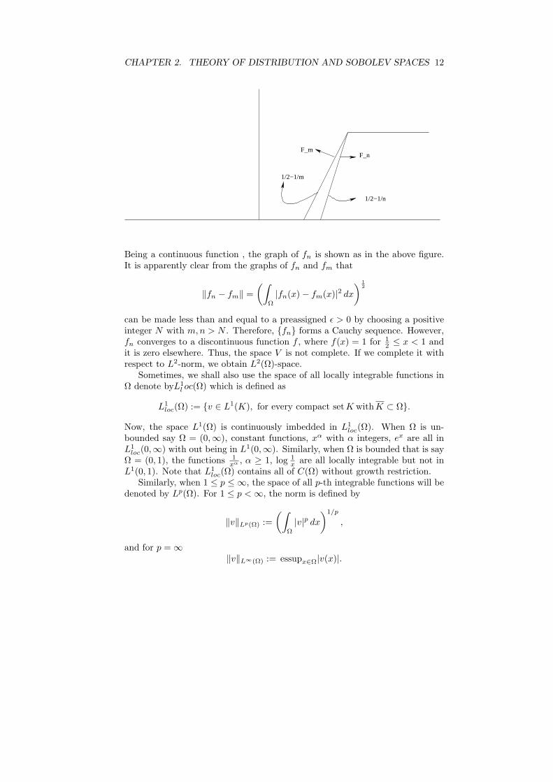
to L2-norm. We can now recall one example in our analysis course. Consider asequence fnn≥2 of continuous functions in C(0, 1) asthat is each fn ∈ C(0, 1) and

fn(x) =

1, 1

2 ≤ x < 10, 0 < x ≤ 1

2 − 1n .

1The identity map i : C(Ω) 7→ L2(Ω) is continuous that is ‖v‖ ≤ Cmaxx∈Ω

|v(x)|.


1/2−1/m

1/2−1/n

F_nF_m

Being a continuous function , the graph of fn is shown as in the above figure.It is apparently clear from the graphs of fn and fm that

‖fn − fm‖ =

(∫Ω

|fn(x)− fm(x)|2 dx) 1

2

can be made less than and equal to a preassigned ε > 0 by choosing a positiveinteger N with m,n > N . Therefore, fn forms a Cauchy sequence. However,fn converges to a discontinuous function f , where f(x) = 1 for 1

2 ≤ x < 1 andit is zero elsewhere. Thus, the space V is not complete. If we complete it withrespect to L2-norm, we obtain L2(Ω)-space.

Sometimes, we shall also use the space of all locally integrable functions inΩ denote byL1

l oc(Ω) which is defined as

L1loc(Ω) := v ∈ L1(K), for every compact setK withK ⊂ Ω.

Now, the space L1(Ω) is continuously imbedded in L1loc(Ω). When Ω is un-

bounded say Ω = (0,∞), constant functions, xα with α integers, ex are all inL1loc(0,∞) with out being in L1(0,∞). Similarly, when Ω is bounded that is say

Ω = (0, 1), the functions 1xα , α ≥ 1, log 1

x are all locally integrable but not inL1(0, 1). Note that L1

loc(Ω) contains all of C(Ω) without growth restriction.Similarly, when 1 ≤ p ≤ ∞, the space of all p-th integrable functions will be

denoted by Lp(Ω). For 1 ≤ p <∞, the norm is defined by

‖v‖Lp(Ω) :=

(∫Ω

|v|p dx)1/p

,

and for p = ∞‖v‖L∞(Ω) := essupx∈Ω|v(x)|.


2.2 A Quick Tour to the Theory of Distribu-tions.

We would like to generalize the concept of differentiation to the functions be-longing to a really large space. One way to catch hold of such a space is toconstruct a smallest nontrivial space and then take its topological dual. As apreparation to choose such a space, we recall some notations and definitions.

A multi-index α = (α1, · · · , αd) is a d-tuple with nonnegative integer ele-

ments. By an order of α, we mean |α| =∑d

i=1 αi. The notion of multi-indexis very useful for writing the higher order partial derivatives in compact form.Define αth order partial derivative of v as

Dαv =∂|α|v

∂xα11 , · · · , ∂xαd

d

, α = (α1, · · · , αd).

Example 2.1. When d = 3 and α = (1, 2, 1) with |α| = 4, the

Dαv =∂4v

∂x1∂x22∂x3.

In case |α| = 2, we have the following 6 possibilities :(2, 0, 0), (1, 1, 0), (0, 2, 0),(0, 1, 1), (0, 0, 2), (1, 0, 1) and Dα will represent all the partial derivatives oforder 2. When α ≤ 3, Dα would mean all partial derivatives up and including3.

Let Cm(Ω) := v : Dαv ∈ C(Ω), |α| ≤ m. Similarly, we define the spaceCm(Ω) as m-times continuously differentiable functions with uniformly con-tinuous derivatives up to order m. By C∞(Ω), we mean a space of infinitelydifferentiable functions in Ω, i.e., C∞(Ω) = ∩Cm(Ω) . The support of a functionv called supp v is defined by

supp v := x ∈ Ω : v(x) 6= 0.

If this set is compact ( i.e., if it is bounded in this case) and supp v ⊂⊂ Ω,then v is said to have ‘compact support’ with respect to Ω. Denote by C∞

0 (Ω),a space of all infinitely differentiable functions with compact support in Ω. Infact, this is a nonempty set and it can be shown as has been done below that ithas as many elements as the points in this set Ω.Example 2.2. For Ω = IR, consider the function

φ(x) =

exp( 1

|x|2−1 ), |x| < 1,

0, |x| ≥ 1.

In order to show that φ ∈ C∞0 (Ω), it is enough to check the continuity and

differentiability properties only at the points x = ±1. Apply L’Hopsital rule toconclude the result.

Similarly, when Ω = IRd, consider


φ(x) =

exp( 1

‖x‖2−1 ), ‖x‖ < 1,

0, ‖x‖ ≥ 1,

where ‖x‖2 =∑d

i=1 |xi|2. Then, since the function is radial, we can in a similarmanner prove that φ ∈ C∞

0 (Ω). For all other points we can simply translateand show the existence of such a function.Exersise 2.1 Show that φ ∈ C∞

0 (IRd)When Ω is a bounded domain in IRd, consider for any point x0 ∈ Ω and

small ε > 0 the following function

φε(x) =

exp( ε

‖x−x0‖2−ε ), ‖x− x0‖ < ε,

0, ‖x− x0‖ ≥ ε.

This function has the desired property and can be constructed for each and everypoint in the domain. Since the domain Ω is open, it is possible to find ε for pointx0 ∈ Ω so that the the ε-ball around x0 is inside the domain. Therefore, thespace C∞

0 (Ω) is a nontrivial vector space and this is the smallest space we arelooking for. In order to consider the topological dual of this space, we need toequip C∞

0 (Ω) with a topology with respect to which we can discuss convergenceof a sequence. Since we shall be only using the concept of convergence of asequence to discuss the continuity of the linear functionals defined on C∞

0 (Ω),we refrain from defining the topology. We say :

‘There is a structure (topology) on C∞0 (Ω) with respect to which the con-

vergence of a sequence φn to φ has the following meaning, i.e., φn 7→ φ inC∞

0 (Ω) if the following conditions are satisfied

(i) there is a common compact set K in Ω with K ⊂ Ω such that

supp φn, supp φ ⊂ K.

(ii) Dαφn 7→ Dαφ uniformly in K, for all multi-indices α.

When C∞0 (Ω) is equipped with such a topology, we call it D(Ω), the space of

test functions. Definition. A continuous linear functional on D(Ω) is calleda distribution, i.e., T : D(Ω) 7→ IR is called a distribution if T is linear andT (φn) 7→ T (φ) as φn 7→ φ in D(Ω). The space of all distributions will be denotedby D′(Ω). This is the topological dual of D(Ω).

We shall use < ·, · > for duality pairing between D′(Ω) and D(Ω).Example 2.3. Every integrable function defines a distribution.

Let f ∈ L1(Ω). Then for φ ∈ D(Ω), set Tf as

Tf (φ) =

∫Ω

fφ dx.

We now claim that Tf ∈ D′(Ω). Linearity of Tf is a consequence of additivity aswell as homogeneity property of the integral. It, therefore, remains to show that


Tf is continuous, i.e., as φn 7→ φ in D(Ω), we need to prove Tf (φn) 7→ Tf (φ).Note that

|Tf (φn)− Tf (φ)| =∣∣∣∣∫

Ω

f(φn − φ) dx

∣∣∣∣ .Since φn converges to φ in D(Ω), there is a common compact set K in Ω suchthat supp φn, supp φ ⊂ K and φn 7→ φ uniformly in K. Therefore,

|Tf (φn)− Tf (φ)| ≤∫K

|f(φn − φ)| dx ≤ maxx∈K

|φn(x)− φ(x)|∫Ω

|f | dx.

Since∫Ω|f | dx <∞, Tf (φn) 7→ Tf (φ), as n 7→ ∞ and the result follows.

If f and g are in L1(Ω) with f = g a.e., then Tf = Tg. Thus, we identifyTf = f and Tf (φ) =< f, φ >. Therefore, L1(Ω) ⊂ D′(Ω).

Excercise 2.1. Show that every square integrable function defines a distribution.Excercise 2.2. Prove that every locally integrable function defines a distribution.

Example 2.4. The Dirac delta δ function ( it is a misnomer and it is a func-tional, but in literature it is still called a function as P. A. M. Dirac called thisa function when he discovered it) concentrated at the origin (0 ∈ Ω) is definedby

δ(φ) = φ(0), ∀φ ∈ D(Ω).

This, in fact, defines a distribution. Linearity is trivial. As φn 7→ φ in D(Ω),i.e., φn 7→ φ uniformly on a common compact support, then,

δ(φn) = φn(0) 7→ φ(0) = δ(φ), ∀φ ∈ D(Ω).

Therefore, δ ∈ D′(Ω) and we write δ(φ) =< δ, φ >= φ(0).Note that the Dirac delta function can not be generated by locally integrablefunction ( the proof can be obtained by using arguments by contradiction 2).Therefore, depending on whether the distribution is generated by locally inte-grable function or not, we have two types of distributions: Regular and Singulardistributions.

(i) Regular. The distributions which are generated by locally integrable func-tions.

2Suppose that the Dirac delta is genereted by a locally integreble function say f . Thenwe define the distribution Tf (φ) = δ(φ) that is Tf (φ) = φ(0) for φ ∈ D(IRd). For ε > 0 it is

possible to find φε ∈ D(IRd) with suppφε ⊂ Bε(0), 0 ≤ φε ≤ 1 and φε ≡ 1 in Bε/2(0). Notethat δ(φε) = 1. But on the other hand

δ(φε) = Tf (φε) =

∫IRd

fφε dx =

∫Bε(0)

fφε dx ≤∫Bε(0)

|f |dx.

Since f is localy integrable ,∫Bε(0)

|f |dx −→ 0 as ε −→ 0, that is δ(φε) −→ 0. This leads to

a contradiction and hence the Direc delta function can not be genereted by locally integrablefunctions


(ii) Singular. The distributions is called singular if it is not regular. Forexample, the Dirac delta function is a singular distribution.

Note that if T1, T2 ∈ D′(Ω) are two regular distributions satisfying

< T1, φ >=< T2, φ > ∀φ ∈ D(Ω),

then T1 = T2. This we shall not prove , but like to use it in future3

We can also discuss the convergence of the sequence of distributions Tn toT in D′(Ω). Say, Tn 7→ T in D′(Ω) if

< Tn, φ >7→< T, φ >, ∀φ ∈ D(Ω).

As an example, we consider ε > 0

ρε(x) =

Aε−d exp

(−ε2

ε2−‖x‖2

)φ(x), ‖x‖ < ε,

0, ‖x‖ ≥ ε,

where A−1 =∫‖x‖≤1

exp(

−11−‖x‖2

)dx. Note that

∫IRd ρε dx = 1. It is easy to

check that ρε ∈ D′(IRd). We now claim that ρε −→ δ in D′(IRd) as ε −→ 0. Forφ ∈ D(IRd), we note that

〈ρε, φ〉 = Aε−d

∫IRd

exp

(−ε2

ε2 − ‖x‖2

)φ(x) dx.

= A

∫IRd

exp

(−1

1− ‖y‖2

)φ(εy) dy

= φ(0) +A

∫IRd

exp

(−1

1− ‖y‖2

)(φ(εy)− φ(0)) dy.

As ε −→ 0, using the Lebesgue dominated convergence theorem, we can takethe limit under the integral sign and therefor, the integral term become zero.Thus we obtain

limε〈ρε, φ〉 = φ(0) = 〈δ, φ〉.

Hence the result follows.Distributional Derivatives. In order to generalize the concept of differen-tiation, we note that for f ∈ C1([a, b]) and φ ∈ D([a, b]), integration by partsyields ∫ b

a

f ′(x)φ(x) dx = fφ|x=bx=a −

∫ b

a

f(x)φ′(x) dx.

Since supp φ ⊂ (a, b), φ(a) = φ(b) = 0. Thus,∫ b

a

f ′(x)φ(x) dx = −∫ b

a

f(x)φ′(x) dx = − < f, φ′ >, ∀φ ∈ D(Ω).

3This is a cosequence of the following Lebesque lemma: Le Tf and Tg are two regulardistribution genereted by locally integrable functions f and g, respectively. Then Tf = Tg ifand only if f = g a.e.


We observe that the meaning of derivative of f can be attached through theterm on the right hand side. However, the term on the right hand side is stillbe meaningful even if f is not differentiable. Note that f can be a distribution.This motivates us to define a derivative of a distribution.

If T ∈ D′(Ω) (Ω = (a, b)), then define DT as

(DT )(φ) = − < T,Dφ >, ∀ φ ∈ D(Ω).

Here, Dφ is simply the derivative of φ. Observe that (DT ) is a linear map. Forφ1, φ2 ∈ D(Ω) and a ∈ IR,

(DT )(φ1 + aφ2) = − < T,D(φ1 + aφ2) >

= − < T,Dφ1 > −a < T,Dφ2 >

= (DT )(φ1) + a(DT )(φ2).

For continuity, we first infer that as φn → φ in D(Ω), Dφn → Dφ on D(Ω).Now,

(DT )(φn) = − < T,Dφn >→ − < T,Dφ >= (DT )(φ).

Therefore, DT ∈ D′(Ω).More precisely, if T is a distribution, i.e., T ∈ D′(Ω), then αth order distri-

butional derivative, say DαT ∈ D′(Ω), is defined by

< DαT, φ >= (−1)α < T,Dαφ >, φ ∈ D(Ω).

Example 2.5. Let Ω = [−1, 1] and let f = |x| in Ω. Obviously, f ∈ D′(−1, 1).To find its distributional derivative Df , write first for φ ∈ D(Ω)

< Df, φ > = − < f,Dφ >

= −∫ 1

−1

f(x)φ′(x)dx

= −∫ 0

−1

(−x)φ′(x)dx−∫ 1

0

xφ′(x)dx.

On integrating by parts and using φ(1) = φ(−1) = 0, it follows that

< Df, φ > = xφ]0−1 −∫ 0

−1

φ(x)dx− xφ]10 +

∫ 1

0

φ(x)dx

=

∫ 1

−1

(−1)φ(x)dx+

∫ 1

0

1φ(x)dx

=

∫ 1

−1

H(x)φ(x)dx

= < H,φ >, ∀ φ ∈ D(Ω),

where

H(x) =−1, −1 < x < 01. 0 ≤ x < 1


As < Df, φ >=< H,φ >, ∀φ ∈ D(Ω), we obtain Df = H. The first distribu-tional derivative of f is a Heaviside step function.

Again to find DH, note that

< DH,φ > = − < H,Dφ >= −∫ 1

−1

H(x)φ′(x)dx

=

∫ 0

−1

φ′(x)dx−∫ 1

0

φ′(x)dx

= φ(0)− φ(−1)− φ(1) + φ(0)

= 2φ(0) = 2 < δ, φ > .

Therefore,DH = 2δ or D2f = 2δ.

In the above example, we observe that if a locally integrable function has aclassical derivative a.e., which is also locally integrable, then then the classicalderivative may not be equal to the distributional derivative. However, if afunction is absolute continous, then its classical derivative coincides with itsdistributional derivative.Exercises:

1.) Find Df , when

f(x) =

1, 0 ≤ x < 10, −1 < x < 0

f(x) = log x, 0 < x < 1, f(x) = (log 1x )

k, k < 12 .

2.) Find Df , when f(x) = sin ( 1x ), 0 < x < 1 and

f(x) = 1x , 0 < x < 1.

3.) Find D2f when f(x) = x|x|, −1 < x < 1.

For Ω ⊂ IRd, let f ∈ C1(Ω) and φ ∈ D(Ω). Then using integration by parts, wehave ∫

Ω

∂f

∂xiφdx = −

∫Ω

f∂φ

∂xidx = − < f,Diφ > .

As in one variable case, set the first generalized partial derivative of a distribu-tion T ∈ D′(Ω) as

< DiT, φ >= − < T,Diφ >, ∀φ ∈ D(Ω).

It is easy to check that DiT ∈ D′(Ω). Similarly, if T ∈ D′(Ω) and α is a multi-index, then the αth order distributional derivative DαT ∈ D′(Ω) is defined by

< DαT, φ >= (−1)|α| < T,Dαφ >, ∀φ ∈ D(Ω).


Example 2.6. Let Ω = (x1, x2) ∈ IR2 : x21 + x22 < 1. Set radial functionf(r) = (log 1

r )k, k < 1

2 , where r =√x21 + x22 < 1. This function is not continu-

ous at the origin, but we shall show that it is in L2(Ω). Now using coordinatetransformation (transforming to polar coordinates), we find that∫

Ω

|f |2 dx1dx2 = π

∫ 1

0

|f(r)|2r dr.

This integral is finite, because r(log( 1r ))2k 7→ 0 as r 7→ 0. Hence, it defines a

distribution. Its partial distributional derivatives may be found out as Dif =∂f∂xi

= −k(log( 1r ))k−1 xi

r2 i = 1, 2.The derivative map Dα : D′ → D′ is continuous. To prove this, let Tn a

sequence in D′ converge to T in D′. Then, for φ ∈ D

< DαTn, φ > = (−1)|α| < Tn, Dαφ >

→ (−1)|α| < T,Dαφ >

= < DαT, φ > .

Hence, the result follows.

2.3 Elements of Sobolev Spaces

We define the (Hilbert) Sobolev space H1(Ω) as the set of all functions in L2(Ω)such that all its first partial distributional derivatives are in L2(Ω), i.e.,

H1(Ω) = v ∈ L2(Ω) :∂v

∂xi∈ L2(Ω), 1 ≤ i ≤ d.

Note that v being an L2(Ω)-function, all its partial distribuitional derivativesexist. But for H1(Ω) what more we require is that ∂v

∂xi∈ L2(Ω), 1 ≤ i ≤ d.

This is, indeed, an extra condition and it is not true that every L2-function hasits first distributional partial derivatives in L2. In the second part of Example2.5, we have shown that DH = 2δ /∈ L2(−1, 1), where as H ∈ L2(−1, 1).

Let us define a map (·, ·)1 : H1(Ω)×H1(Ω) → IR by

(u, v)1 = (u, v) +d∑

i=1

(∂u

∂xi,∂v

∂xi), ∀u, v ∈ H1(Ω). (2.1)

It is a matter of an easy exercise to check that (·, ·)1 forms an inner-product onH1(Ω), and (H1(Ω), (·, ·)1) is an inner-product space. The induced norm ‖ · ‖1on H1(Ω) is set as

‖u‖1 =√

(u, u)1 =

√√√√‖u‖2 +d∑

i=1

‖ ∂u∂xi

‖2. (2.2)

In the next theorem, we shall prove that H1(Ω) is complete.


Theorem 2.1 The space H1(Ω) with ‖ · ‖1 is a Hilbert space.

Proof. Consider an arbitrary Cauchy sequence un inH1(Ω). We claim that itconverges to an element in H1(Ω). Given a Cauchy sequence un in H1(Ω), theun and ∂un

∂xi, i = 1, 2, . . . , d are Cauchy in L2(Ω). Since L2(Ω) is complete,

we can find u and ui, (i = 1, 2, . . . , d) such that

un → u in L2(Ω),

∂un∂xi

→ ui, 1 ≤ i ≤ d, in L2(Ω).

To complete the proof, it is enough to show that ui = ∂u∂xi

. For φ ∈ D(Ω),consider

<∂un∂xi

, φ > = − < un,∂φ

∂xi>= −

∫Ω

un∂φ

∂xidx

→ −∫Ω

u∂φ

∂xidx = − < u,

∂φ

∂xi>

= <∂u

∂xi, φ > .

However,

<∂un∂xi

, φ > =

∫Ω

∂un∂xi

φdx

→∫Ω

uiφdx =< ui, φ > .

Thus,

< ui, φ >=<∂u

∂xi, φ >, ∀φ ∈ D(Ω),

and we obtain

ui =∂u

∂xi.

Therefore,

un → u in L2(Ω) and∂un∂xi

→ ∂u

∂xiin L2(Ω),

i.e.,un → u in H1(Ω).

Since un is arbitrary, we have shown the completeness of H1(Ω).For positive integerm, we also define the higher order Sobolev spacesHm(Ω)

asHm(Ω) := v ∈ L2(Ω) : Dαv ∈ L2(Ω), |α| ≤ m.


This is again a Hilbert space with respect to the inner product

(u, v)m :=∑

|α|≤m

(Dαu,Dαv),

and the induced norm

‖u‖m := (∑

|α|≤m

‖Dαu‖2)1/2.

In fact, it is a matter of an easy induction on m to show that Hm(Ω) is acomplete innerproduct space.

Why should we restrict ourselves to L2-setting alone, we can now defineSobolev spaces Wm,p(Ω) of order (m, p), 1 ≤ p ≤ ∞ by

Wm,p(Ω) := v ∈ Lp(Ω) : Dαv ∈ Lp(Ω), |α| ≤ m.

This is a Banach space with norm

‖u‖m,p :=

∑|α|≤m

∫Ω

|Dαu|p dx

1/p

, 1 ≤ p <∞,

and for p = ∞‖u‖m,∞ := max

|α|≤m‖Dαu‖L∞(Ω).

When p = 2, we shall call, for simplicity, Wm,2(Ω) as Hm(Ω) and its norm‖ · ‖m,2 as ‖ · ‖m.

Exercise 2.2 Show that W 1,p(Ω), (1 ≤ p ≤ ∞) is a Banach space and the usingmathematical induction show that Wm,p(Ω) is also a Banach space.

Some Properties of H1- Space. Below, we shall discuss both negative andpositive properties of H1- Hilbert Sobolev space.Negative Properties.

(i) For d > 1, the functions in H1(Ω) may not be continuous.

In Example 2.6 , we have noted that the function f(r) is not continuousat the origin, but it has distributional derivatives of all order. Now,

∂f

∂xi= −k(log(1

r))k−1 xi

r2, i = 1, 2,

and hence,∫Ω

| ∂f∂x1

|2 dxdy = 4

∫ π/2

0

∫ 1

0

k2(log(

1

r)

)2(k−1)1

rcos2 θ drdθ

= πk2∫ 1

0

r−1

(log(

1

r)

)2(k−1)

dr.


Here, we have used change of variables : x1 = r cos θ, x2 = sin θ, 0 ≤ θ ≤π. It is easy to check that the integral is finite provided k < 1

2 (only care

is needed at r = 0). Therefore, ∂f∂x1

∈ L2(Ω). Similarly, it can be shown

that ∂f∂x2

∈ L2(Ω) and hence, f ∈ H1(Ω).

When d = 1, i.e., Ω ⊂ IR, then every function in H1(Ω) is absolutelycontinuous. This can be checked easily as

u(x)− u(x0) =

∫ x

x0

Du(τ) dτ, x0, x1 ∈ Ω,

where Du is the distributional derivative of u.

(ii) The space D(Ω) is not dense in H1(Ω). To see this, we claim that theorthogonal complement of D(Ω) in H1(Ω) is not a trivial space. Letu ∈ (D(Ω))⊥ in H1(Ω) and let φ ∈ D(Ω). Then

0 = (u, φ)1 = (u, φ) +d∑

i=1

(∂u

∂xi,∂v

∂xi)

= < u, φ > −d∑

i=1

<∂2u

∂x2i, φ >

= < −∆u+ u, φ >, ∀φ ∈ D(Ω).

Therefore,−∆u+ u = 0, inD′(Ω).

We shall show that there are enough functions satisfying the above equa-tion. Let Ω be a unit ball in IRd. Consider u = er·x with r ∈ IRd. Notethat

∆u = |r|2er·x =

|r|2u,u, |r| = 1.

When d = 1, the solution u with r = ±1 belongs to (D(Ω))⊥. For d > 1,there are infinitely many r’s lying on the boundary of the unit ball in IRd

for which u ∈ (D(Ω))⊥. Therefore, the space D(Ω) is not dense in H1(Ω).

One then curious to know :

‘What is the closure of D(Ω) in H1(Ω)-space ?’

Then

‘Is it possible to characterize such a space?’

Let H10 (Ω) be the closure of D(Ω) in H1(Ω)-space. This is a closed sub-

space of H1(Ω). The characterization of such a space will require theconcept of values of the functions on the boundary or the restrictionof functions to the boundary ∂Ω. Note that the boundary ∂Ω being a(d− 1)-dimensional manifold is a set of measure zero, and hence, for any


v ∈ H1(Ω), its value at the boundary or its restriction to the boundary∂Ω does not make sense.

When Ω is a bounded domain with Lipschitz continuous boundary ∂Ω (i.e., the boundary can be parametrized by a Lipschitz function), then thespace C1(Ω) (in fact C∞(Ω)) is dense in H1(Ω). The proof, we shall notpursue it here, but refer to Adams [1]. For v ∈ C1(Ω), its restriction tothe boundary or value at the boundary is meaningful as v ∈ C(Ω). SinceC1(Ω) is dense in H1(Ω), for every v ∈ H1(Ω) there is a sequence vnin C1(Ω) such that vn 7→ v in H1(Ω). Thus, for each vn, its restriction tothe boundary ∂Ω that is vn|∂Ω makes sense and further, vn|∂Ω ∈ L2(∂Ω).This sequence, infact, converges in L2(∂Ω) to an element say γ0v. Thisis what we call the trace of v. More precisely, we define the trace γ0 :H1(Ω) 7→ L2(∂Ω) as a continuous linear map satisfying

‖γ0v‖L2(∂Ω) ≤ C‖v‖1,

and for v ∈ C1(Ω), γ0v = v|∂Ω. This is, indeed, a generalization of theconcept of the values of H1-functions on the boundary or the restrictionto the boundary. The range of γ0 called H1/2(∂Ω) is a proper and densesubspace of L2(∂Ω). The norm on this space is defined as

‖g‖1/2,∂Ω = inf‖v‖1 : v ∈ H1(Ω) and γ0v = g.

Now the space H10 (Ω) is characterized by

H10 (Ω) := v ∈ H1(Ω) : γ0v = 0.

For a proof, again we refer to Adams [1]. Sometimes, by abuse of language,we call γ0v = 0 as simply v = 0on ∂Ω.

Positive Properties of H10 and H1- Spaces. We shall see subsequently that the

denseness of D(Ω) and C∞(Ω), respectively in H10 (Ω) and H

1(Ω) with respectto H1-norm will play a vital role. Essentially, many important results are firstderived for smooth functions and then using the denseness property are carriedover to H1

0 or H1-spaces.In the following, we shall prove some inequalities. If v ∈ V := w ∈ C1[a, b] :

w(a) = w(b) = 0, then for x ∈ [a, b]

v(x) =

∫ x

a

dv

dx(s) ds.

A use of Holder’s inequality yields

|v(x)| ≤ (x− a)1/2(

∫ b

a

|dvdx

|2 ds)1/2.


On squaring and again integrating over x from a to b, it follows that∫ b

a

|v(x)|2 dx ≤ (

∫ b

a

(x− a) dx)(

∫ b

a

|dvdx

|2 ds)

≤ (b− a)2

2

∫ b

a

|dvdx

|2 dx.

Thus,‖v‖L2(a,b) ≤ C(a, b)‖v′‖L2(a,b),

where the constant C(a, b) = (b−a)√2

. This is one dimensional version of Poincare

inequality. We note that in the above result only v(a) = 0 is used. The sameconclusion is also true when v(b) = 0. Further, it is easy to show that

maxx∈[a,b]

|v(x)| ≤ (b− a)1/2‖v′‖L2(a,b).

As a consequence of the Poincare inequality, ‖v′‖L2(a,b) defines a norm on Vwhich is equivalent to H1(a, b)-norm, i.e., there are positive constants say C1

and C2 such thatC1‖v‖1 ≤ ‖v′‖L2(a,b) ≤ C2‖v‖1,

Where C2 = 1 and C1 = ( (b−a)2

2 + 1)−1/2.We shall now generalize this to the functions in H1

0 (Ω), when Ω is a boundeddomain in IRd.

Theorem 2.3 (Poincare Inequality). Let Ω be a bounded domain in IRd. Thenthere exists constant C(Ω) such that∫

Ω

|v|2 dx ≤ C(Ω)

∫Ω

|∇v|2 dx, ∀v ∈ H10 (Ω).

Proof. Since D(Ω) is dense in H10 (Ω), it is enough to prove the above inequality

for the functions in D(Ω). Now because of denseness, for every v ∈ H10 (Ω), there

is a sequence vn in D(Ω) such that vn 7→ v in H1-norm. Suppose for everyvn in D(Ω), the above result holds good,i.e.,∫

Ω

|vn|2 dx ≤ C(Ω)

∫Ω

|∇vn|2 dx, vn ∈ D(Ω), (2.3)

then taking limit as n 7→ ∞, we have ‖vn‖ 7→ ‖v‖ as well as ‖∇vn‖ 7→ ‖∇v‖,and hence, the result follows for v ∈ H1

0 (Ω).It remains to prove (2.3). Since Ω is bounded, enclose it by a box in IRd,

i.e., say Ω ⊂ Πdi=1[ai, bi]. Then extend each vn even alongwith its first partial

derivatives to zero outside of Ω. This is possible as vn ∈ D(Ω). Now, we have(like in one dimensional case) for x = (x1, · · · , xi, · · · , xd)

vn(x) =

∫ xi

ai

∂vn∂xi

(x1, · · · , xi−1, s, xi+1, · · · , xd) ds.


Then using Holder’s inequality

|vn(x)| ≤ (xi − ai)1/2

(∫ bi

ai

|∂vn∂xi

|2 ds

)1/2

.

Squaring and then integrating both sides over the box, it is found that∫ b1

a1

· · ·∫ bd

ad

|vn(x)| dx ≤ (bi − ai)2

2

∫ b1

a1

· · ·∫ bd

ad

|∂vn∂xi

|2 dx.

Therefore the estimate (2.3) follows with the constant C = 12 (bi − ai)

2. Thiscompletes the rest of the proof.Remarks. The above theorem is not true if v ∈ H1(Ω) (say, when Ω = (0, 1)and v = 1, v ∈ H1(Ω) and it does not satisfy Poincare ineguality) or if Ω isnot bounded. But when Ω is within a strip , the result still holds (the proofof theorem only uses that the domain is bounded in one direction that is inthe direction of xi). The best constant C(Ω) can be 1

λmin, where λmin is the

minimum positive eigenvalue of the following Dirichlet problem

−∆u = λu, x ∈ Ω

with Dirichlet boundary condition

u = 0, on ∂Ω.

Using the Poincare inequality , it is easy to arrive at the following result.

Corollary 2.4 For v ∈ H10 (Ω), ‖∇v‖ is, infact, a norm on H1

0 (Ω)-space whichis equivalent to H1-norm.

Using the concept of trace and the denseness property, we can generalize theGreen’s formula to the functions in Sobolev spaces. For details , see Kesavan[9]

Lemma 2.5 Let u and v be in H1(Ω). Then for 1 ≤ i ≤ d, the followingintegration by parts formula holds∫

Ω

u∂v

∂xidx = −

∫Ω

∂u

∂xiv dx+

∫∂Ω

uvνi ds, (2.4)

where νi is the ith component of the outward normal ν to the boundary ∂Ω.Further, if u ∈ H2(Ω), then the following Green’s formula holds

d∑i=1

∫Ω

∂u

∂xi

∂v

∂xidx = −

d∑i=1

∫Ω

∂2u

∂x2iv dx+

d∑i=1

∫∂Ω

νiγ0(∂u

∂xi)γ0(v) ds,

or in usual vector notation

(∇u,∇v) = (−∆u, v) +

∫∂Ω

∂u

∂νv ds. (2.5)


We now state another useful property of H1-space. For a proof, we may referto Adams [1].

Theorem 2.6 ( Imbedding Theorem ). Let Ω be a bounded domain with Lips-chitz boundary ∂Ω. Then H1(Ω) is continuously imbedded in Lp(Ω) for 1 ≤ p <q if d = 2 or p ≤ q, for d ≥ 2, where 1

q = 12 − 1

d . Further, the above imbeddingis compact provided p < q.

Dual Spaces of H1 and H10 . We denote by H−1(Ω), the dual space of H1

0 (Ω),i.e., it consists of all continuous linear functionals on H1

0 (Ω). The norm onH−1(Ω) is given by the standard dual norm and now is denoted by

‖f‖−1 = sup0 6=v∈H1

0 (Ω)

| < f, v > |‖v‖1

. (2.6)

The following Lemma characterizes the elements in the dual space H−1(Ω).

Lemma 2.7 A distribution f ∈ H−1(Ω) if and only if there are functions fα ∈L2(Ω) such that

f =∑|α|≤1

Dαfα. (2.7)

For an example, the Dirac delta function δ belongs to H−1(−1, 1), because thereexists Heaviside step function

H(x) =

1, 0 < x < 1,0, −1 < x ≤ 0

in L2(−1, 1) such that δ = DH.Note that

H10 (Ω) ⊂ L2(Ω) ⊂ H−1(Ω).

In fact the imbedding is continuous in each case. This forms a Gelfand triplet.For f ∈ L2(Ω) and v ∈ H1

0 (Ω), we have the following identification

< f, v >= (f, v), (2.8)

where < ·, · > is a duality pairing between H−1(Ω) and H10 (Ω).

Similarly, we can define the dual space (H1(Ω))′ of H1(Ω). Its norm is againgiven through the dual norm and is defined by

‖f‖(H1(Ω))′ = sup0 6=v∈H1(Ω)

| < f, v > |‖v‖1

. (2.9)

In the present case, we may not have a characterization like the one in theprevious Lemma.


Remark. For positive integer m, we may define Hm0 (Ω) as the closure of D(Ω)

with respect to the norm ‖ · ‖m. For smooth boundary Ω, we can characterizethe space H2

0 by

H20 (Ω) := v ∈ H2(Ω) : γ0v = 0, γ0(

∂v

∂ν) = 0. (2.10)

Similarly, the dual space H−m(Ω) is defined as the set of all distributions fsuch that there are functions fα ∈ L2(Ω) with f =

∑|α|≤mDαfα. The norm is

given by

‖f‖−m = sup0 6=v∈Hm

0 (Ω)

| < f, v > |‖v‖m

. (2.11)

Note. There are some exellent books available on the theory of Distributionand Sobolev Spaces like Adams [1], Dautray and Lions [5]. In this chapter, wehave discussed only the basic rudiment theory which is barerly minimum for thedevelopment of the subsequent chapters.

Chapter 3

Abstract Elliptic Theory

We present in this chapter a brief account of the fundamental tools whichare used in the study of linear elliptic partial differential equations. To motivatethe materials to come, we again start with the mathematical model of vibrationof drum: Find u such that

−∆u = f in Ω (3.1)

u = 0 on ∂Ω, (3.2)

where Ω ⊂ IRd (d = 2, 3) is a bounded domain with smooth boundary ∂Ω andf is a given function.

Multiply (3.1) by a nice function v which vanishes on ∂Ω (say v ∈ D(Ω))and then integrate over Ω to obtain∫

Ω

(−∆u)vdx =

∫Ω

fvdx.

Formally, a use of Gauss divergence theorem for the integral on the left handside yields ∫

Ω

(−∆u)vdx = −∫∂Ω

∂u

∂νvds+

∫Ω

∇u · ∇vdx.

Since v = 0 on ∂Ω, the first term on the right hand side vanishes and hence, weobtain ∫

Ω

∇u · ∇vdx =

∫Ω

fvdx.

Therefore, the problem (3.1) is reformulated as: Find a function u ∈ V suchthat

a(u, v) = L(v), ∀v ∈ V, (3.3)

where a(u, v) =∫Ω∇u · ∇vdx, and L(v) =

∫Ωfvdx. Here, the space V (the

space of all admissable displacements for the problem (1.1)) has to be chosenapproprietely. For the present case, one thing is quite apparent that everyelement of V should vanish on ∂Ω.

28

CHAPTER 3. ABSTRACT ELLIPTIC THEORY 29

How does one choose V ? The choice of V should be such that the integralsin (3.3) are finite. For f ∈ L2(Ω), space V may be chosen in such a waythat ∇u ∈ L2(Ω) and u ∈ L2(Ω). The largest such space satisfying the aboveconditions and u = 0 on ∂Ω is, in fact, the space H1

0 (Ω). Thus, we chooseV = H1

0 (Ω). Since D(Ω) is dense in H10 (Ω), the problem (3.3) makes sense for

all v ∈ V .Now, observe that every (classical) solution of (3.1) – (3.2) satisfies (3.3).

However, the converse need not be true. Then, one is curious to know whether,in some weaker sense, the solution of (3.3) does satisfy (3.1) – (3.2) . To seethis, note that ∫

Ω

∇u · ∇vdx =

∫Ω

fvdx, ∀v ∈ D(Ω) ⊂ H10 (Ω).

Using the definition of distributional derivatives, it follows that∫Ω

∇u · ∇v dx =

d∑i=1

∫Ω

∂u

∂xi

∂v

∂xidx

=d∑

i=1

<∂u

∂xi,∂v

∂xi> = −

d∑i=1

<∂2u

∂x2i, v >

= < −∆u, v > ∀v ∈ D(Ω),

and hence,< −∆u, v >=< f, v > ∀v ∈ D(Ω).

Obviously,−∆u = f in D′(Ω). (3.4)

Thus, the solution of (3.3) satisfies (3.1) in the sense of distribution, i.e., in thesense of (3.4) .

Conversely, if u satisfies (3.4), then following the above steps backward, weobtain

a(u, v) = L(v) ∀v ∈ D(Ω).

As D(Ω) is dense in H10 (Ω), the above equation holds for v ∈ H1

0 (Ω) and hence,u is a solution of (3.3).

Since most of the linear elliptic equations can be recast in the abstract form(3.3), we examine, below, some sufficient conditions on a(·, ·) and L so that theproblem (3.3) is wellposed in the sense of Hadamard.

3.1 Abstract Variational Formulation

Let V and H be real Hilbert spaces with V → H = H ′ → V ′ where V ′ is thedual space of V . Given a continuous linear functional L on V and a bilinearform a(·, ·) : V × V → IR, the abstract variational problem is to seek a functionu ∈ V such that

a(u, v) = L(v) ∀v ∈ V. (3.5)


In the following Theorem, we shall prove the wellposedness of (3.5). This the-orem is due to P.D. Lax and A.N. Milgram (1954) and hence, it is called Lax-Milgram Theorem.

Theorem 3.1 Assume that the bilinear form a(·, ·) : V × V → IR is boundedand coercive, i.e., there exist two constants M and α0 > 0 such that

(i) |a(u, v)| ≤M‖u‖V ‖v‖V ∀u, v ∈ V

and(ii) a(u, v) ≥ α0‖v‖2V ∀v ∈ V.

Then, for a given L ∈ V ′ the problem (3.5) has one and only one solution u inV . Moreover,

‖u‖V ≤ 1

α0‖L‖V ′ , (3.6)

i.e., the solution u depends continuously on the given data L.

Remark: In addition if we assume a(·, ·) is symmetric, then as a consequence ofRiesz-Representation Theorem1, it is easy to show the wellposedness of (3.5).Since a(·, ·) is symmetric, define an innerproduct on V as ((u, v)) = a(u, v). The

introduced norm is |||u||| = ((u, u))12 = (a(u, u))

12 . The space (V, ||| · |||) is a

Hilbert space. Due to boundedness and coercivity of a(·, ·), we have

α0‖v‖2V ≤ ((u, v)) = |||v|||2 ≤M‖v‖2V .

Hence, the two norms are equivalent. Thus, both these spaces have the samedual V ′. Then the problem (3.5) can be reformulated in this new setting as:Given L ∈ V ′, find u ∈ (V, ||| · |||) such that

((u, v)) = L(v) ∀v ∈ V. (3.7)

Now, an application of Riesz-Representation Theorem ensures the existence ofa unique element u ∈ (V, ||| · |||) such that (3.7) is satisfied. Further,

√α0‖u‖V ≤ |||u||| = ‖L‖V ′

and hence, the result follows.When a(·, ·) is not symmetric, we prove the result as follows:

Proof of Theorem 3.1. We shall first prove the estimate (3.6). Using coercivity,the property (ii) of the bilinear form, we have

α0‖u‖2V ≤ a(u, u) = |L(u)| ≤ ‖L‖V ′‖u‖V .

Therefore, the result (3.6) follows. For continuous dependence, let Ln → L inV ′ and let un be the solution of (3.5) corresponding to Ln. Then, using linearityproperty,

a(un − u, v) = (Ln − L)(v).

1For every continuous linear functional l on a Hilbert space V , there exists one and onlyone element u ∈ V such that l(v) = (u, v)V , ∀v ∈ V and ‖u‖V = ‖l‖V ′ .


Now, an application of the estimate (3.6) yields

‖un − u‖V ≤ 1

α0‖Ln − L‖V ′ .

Hence, Ln → L in V ′ implies un → u in V , and this completes the proof of thecontinuous dependence of u on L. Uniqueness is a straight forward consequenceof the continuous dependence.

For existence, we shall put (3.5) in an abstract operator theoretic form andthen apply Banach contraction mapping theorem 2

For w ∈ V , define a functional lw by lw = a(w, v) ∀v ∈ V. Note that lw islinear functional on V . Using boundedness of the bilinear form, we obtain

|lw(v)| = |a(w, v)| ≤M‖w‖V ‖v‖V ,

and hence,

‖lw‖V ′ = supv∈V

|lw(v)|‖v‖V

= supv∈V

|a(w, v)|‖v‖V

≤M‖w‖V <∞.

Thus, lw ∈ V ′. Since w 7→ lw is a linear map, setting A : V → V ′ by Aw = lw,we have

(Aw, v) = a(w, v) ∀v ∈ V.

Indeed, w 7→ Aw is a linear map and A is continuous with ‖Aw‖V ≤ M‖w‖V .Let τ : V ′ 7→ V denote the Riesz mapping such that

∀f ∈ V ′, ∀v ∈ V, f(v) = (τf, v)V ,

where (·, ·)V is the innerproduct in V . The variational problem (3.5) is nowequivalent to the operator equation

τAu = τL in V. (3.8)

Thus, for the wellposedness of (3.5), it is sufficient to show the wellposedness of(3.8). For ρ > 0, define a map J : V → V by

J v = v − ρ (τAv − τL) ∀v ∈ V. (3.9)

Suppose J in (3.9) is a contraction, then by contraction mapping theorem thereis a unique element u ∈ V such that J u = u, i.e., u − ρ (τAu− L) = u and usatisfies (3.8). To complete the proof, we now show that J is a contraction. Forv1, v2 ∈ V , we note that

‖J v1 − v2‖2V = ‖v1 − v2 − ρ (τAv1 − τAv2) ‖2V≤ ‖v1 − v2‖2V − 2ρa(v1 − v2, v1 − v2) + ρ2a(v1 − v2, τA(v1 − v2))

≤ ‖v1 − v2‖2V − 2ρα0‖v1 − v2‖2V + ρ2M2‖v1 − v2‖2V .2A map J : V → V (V can be taken even as a Banach space or even a metric space) is

said to be a contraction if there is a constant 0 ≤ β < 1 such that ‖J u−J v‖V ≤ β‖u− v‖Vfor u, v ∈ V . Every contraction mapping has a unique fixed point, i.e., ∃! u0 ∈ V such thatJ u0 = u0.


Here, we have used the coercive property (ii) and boundedness property of A.Altogether,

‖J v1 − J v2‖2V ≤ (1− 2ρα0 + ρ2M2)‖v1 − v2‖2V ,

and hence,

‖Jw1 − Jw2‖V ≤√

(1− 2ρα0 + ρ2M2)‖w1 − w2‖V .

With a choice of ρ ∈ (0, α0

2M ), we find that J is a contraction and this completesthe proof.Remark. There are also other proofs that are available in the literature. Onedepends on continuation argument by looking at the deformation from the sym-metric case and other depends on the existence of a solution to an abstractoperator equation. However, the present existential proof gives an algorithm tocompute the solution as a fixed point of J . Based on Faedo-Galerkin method,another proof is presented in Temam [11] (see, pages 24–27).

Corollary 3.2 When the bilinear form a(·, ·) in symmetric, i.e., a(u, v) =a(v, u), u, v ∈ V , and coercive, then the solution u of (3.5) is also the onlyelement of V that minimizes the following energy functional J on V , i.e.,

J(u) = minv∈V

J(v), (3.10)

where J(v) = 12a(v, v)− L(v). Moreover, the converse is also true.

Proof. Let u be a solution of (3.5). Write v = u + w, for some vector w ∈ V .Note that

J(v) = J(u+ w) =1

2a(u+ w, u+ w)− L(u+ w)

=1

2a(u, u)− L(u) +

1

2(a(u,w) + a(w, u))− L(w) +

1

2a(w,w).

Using definition of J and symmetric property of a(·, ·), we have

J(v) = J(u) + (a(u,w)− L(w)) +1

2a(w,w) ≥ J(u).

Here, we have used the fact that u is a solution of (3.5) and coercivity (ii) ofthe bilinear form, Since v is arbitrary (it can be done by varying w), u satisfies(3.10).

To prove the converse (direct proof), let u be a solution of (3.10). Define ascalar function for t ∈ IR as

Φ(t) = J(u+ tv).

Indeed, Φ(t) has a minimum at t = 0. If Φ(t) is differentiable, then Φ(t)′|t=0 = 0.Note that

Φ(t) =1

2a(u+ tv, u+ tv)− L(u+ tv)

=1

2a(u, u) +

t

2(a(u, v) + a(v, u)) +

t2

2a(v, v)− L(u)− tL(v).


This is a quadratic functional in t and hence, differentiable. Using symmetricproperty of a(·, ·), the derivative of Φ is

Φ′(t) = a(u, v)− L(v) + ta(v, v), ∀t.

Now Φ′(0) = 0 implies a(u, v) = L(v) ∀v ∈ V , and hence, the result follows.

3.2 Some Examples.

In this section, we discuss some examples of linear elliptic partial differentialequations and derive wellposedness of the weak solutions using Lax-MilgramTheorem. In all the following examples, we assume that Ω is a bounded domainwith Lipschitz continuous boundary ∂Ω.

Example 3.3 (Homogeneous Dirichlet Boundary Value Problem Revisited)

For the problem (3.1)-(3.2), the weak formulation is given by (3.3) in V =H1

0 (Ω) for wellposedness, the bilinear form a(·, ·) satisfies both the properties:

a(v, v) =

∫Ω

|∇v|2 dx = ‖v‖2V ,

and

|a(u, v)| = |∫Ω

∇u · ∇v dx| ≤ ‖u‖V ‖v‖V .

The functional L is linear and using the identification (2.9) in Chapter 2, wehave

L(v) = (f, v) =< f, v > ∀v ∈ V.

Hence, using Poincare inequality it follows that

‖L‖V ′ = sup0 6=v∈V

|L(v)|‖v‖V

≤ C‖f‖.

An application of the Lax-Milgram Theorem yields the wellposedness of (3.3).Moreover,

‖u‖1 ≤ C‖f‖.Since, f ∈ L2(Ω), it is straight forward to check that ‖∆u‖ ≤ ‖f‖ and thefollowing regularity result can be shown to hold

‖u‖2 ≤ C‖f‖.

For a proof, see , Kesavan [9].Since, the bilinear form is symmetric, by Corollary 3.2 the problem (3.3) is

equivalent to the following minimization problem:

J(u) = minv∈H1

0 (Ω)J(v),

where

J(v) =1

2

∫Ω

|∇v|2 dx−∫Ω

fv dx.


Example 3.4 (Nonhomogeneous Dirichlet Problem)

Given f ∈ H−1(Ω) and g ∈ H12 (∂Ω), find a function u satisfying

−∆u = f, x ∈ Ω (3.11)

with non-homogeneous Dirchlet boundary condition

u = g, x ∈ ∂Ω.

To put (3.11) in the abstract variational form, the choice of V is not difficult

to guess. Now since H12 (∂Ω) = Range of γ0, where γ0 : H1(Ω) → H

12 (∂Ω),

then for g ∈ H12 (∂Ω), there is an element say u0 ∈ H1(Ω) such that γ0u0 = g.

Therefore, we recast the problem as: Find u ∈ H1(Ω) such that

u− u0 ∈ H10 (Ω), (3.12)

a(u− u0, v) =< f, v > −a(u0, v) ∀v ∈ H10 (Ω), (3.13)

where a(v, w) =∫Ω∇v · ∇wdx. We obtain (3.13) by using Gauss divergence

Theorem.To check the conditions in the Lax-Milgram Theorem, note that V = H1

0 (Ω),and the bilinear form a(·, ·) satisfies

|a(u, v)| ≤∫Ω

|∇u||∇v| dx ≤ ‖∇u‖‖∇v‖ = ‖u‖V ‖v‖V .

In H10 (Ω), ‖∇u‖ is in fact a norm (see Corollary 2.1) and is equivalent to

H1(Ω)−norm. For coercivity,

a(u, v) =

∫Ω

|∇u|2 dx = ‖u‖2V .

Since a(·, ·) is continuous, the mapping L : v →< f, v > −a(u0, v) is a continu-ous linear map on H1

0 (Ω) and hence, it belongs to H−1(Ω). An application ofLax-Milgram Theorem yields the wellposedness of (3.12)-(3.13). Further,

‖u‖V − ‖u0‖V ≤ ‖u− u0‖V = ‖∇(u− u0)‖ ≤ ‖L‖H−1(Ω) ≤ ‖f‖−1 + ‖∇u0‖.

Therefore, using the equivalence of the norms on H10 (Ω) and H

1(Ω), we obtain

‖u‖1 ≤ c(‖f‖−1 + ‖u0‖1),

for all u0 ∈ H1(Ω) such that γ0u0 = g. However, taking infimum over u0 ∈H1(Ω) for which γ0u0 = g, it follows that

‖u‖1 ≤ C(‖f‖−1 + infu0∈H1(Ω)

‖u0‖1 : γ0u0 = g) = C(‖f‖−1 + ‖g‖ 12 ,∂Ω

),


(using definition of H12 (∂Ω)). It remains to check that in what sense u satisfies

(3.10)-(3.11)? Choose v ∈ D(Ω) in (3.13). This is possible as D(Ω) ⊂ H10 (Ω).

Thena(u, v) = − < ∆u, v >=< f, v > ∀v ∈ D(Ω).

Since f ∈ H−1(Ω), ∆u ∈ H−1(Ω) and hence, u satisfies

u− u0 ∈ H10 (Ω), (3.14)

−∆u = f, in H−1(Ω). (3.15)

Converse part is straight forward as D(Ω) is dense in H10 (Ω). However u−u0 ∈

H10 (Ω) if only if γ0u0 = g and hence, the non-homogeneous boundary condition

is satisfied.Remark. It is even possible to show the following higher regularity result pro-vided f ∈ L2(Ω) and g ∈ H

32 (∂Ω):

‖u‖2 ≤ c(‖f‖+ ‖g‖ 32 ,∂Ω

),

where‖g‖ 3

2 ,∂Ω= inf

v∈H2(Ω)‖v‖2 : γ0v = g.

Since a(·, ·) is symmetric, u− u0 will minimize J(v) over H10 (Ω), where

J(v) =1

2a(v, v)− < f, v > .

Example 3.5 (Neumann Problem): Find u such that

−∆u+ cu = f in Ω, (3.16)

∂u

∂ν= g on ∂Ω. (3.17)

Here assume that f ∈ L2(Ω), g ∈ L2(∂Ω) and c > 0.

To find out the space V , the bilinear form and the linear functional, wemultiply (3.16)-(3.17) by a smooth function v and apply Green’s Formula:∫

Ω

∇u · ∇v dx−∫∂Ω

∂u

∂νv ds+

∫Ω

cuv dx =

∫Ω

fv dx.

Using Neumann boundary condition∫Ω

∇u · ∇v dx+

∫Ω

cuv dx =

∫Ω

fv dx+

∫∂Ω

gv ds. (3.18)

Therefore, set

a(u, v) =

∫Ω

(∇u · ∇v + cuv) dx,


and

L(v) =

∫∂Ω

gv ds+

∫Ω

fv dx.

The largest space for which these integrals are finite is H1(Ω)-space. So wechoose V = H1(Ω). To verify the sufficient conditions in the Lax-MilgramTheorem, note that the bilinear form a(·, ·) satisfies:

(i) the boundedness property as

|a(u, v)| = |∫Ω

(∇u · ∇v + cuv) dx|

≤ ‖∇u‖‖∇v‖+maxx∈Ω

c(x)‖u‖‖v‖

≤ max(1,maxx∈Ω

c(x))‖u‖1‖v‖1.

(ii) the coercive condition, since

a(v, v) =

∫Ω

(‖∇v‖2 + c|v|2) dx ≥ min(1, c)‖v‖21 = α‖v‖21.

Further, L is a linear functional and it satisfies

|L(v)| ≤∫∂Ω

|g||v| ds+∫Ω

|f ||v| dx

≤ ‖g‖L2(∂Ω)‖γ0v‖L2(∂Ω) + ‖f‖‖v‖.

As ‖v‖ ≤ ‖v‖1 and from the trace result ‖γ0v‖L2(∂Ω) ≤ C‖v‖1, we obtain

‖L‖(H1)′ = sup0 6=v∈H1(Ω)

|L(v)|‖v‖1

≤ C(‖f‖+ ‖g‖L2(∂Ω)).

Therefore, L is a continuous linear functional onH1(Ω). Apply the Lax-MilgramTheorem to obtain the wellposedness of the weak solution of (3.18). Moreover,the following regularity also holds true

‖u‖1 ≤ C(‖f‖+ ‖g‖L2(∂Ω)).

Choose v ∈ D(Ω) as D(Ω) ⊂ H1(Ω) and using Green’s formula, we find that

a(u, v) =< −∆u+ cu, v >,

and hence,< −∆u+ cu, v >=< f, v >, ∀D(Ω).

Therefore, the weak solution u satisfies the equation

−∆u+ cu = f, in D′(Ω).


Since f ∈ L2(Ω), −∆u+ cu ∈ L2(Ω). Further, it can be shown that u ∈ H2(Ω).For the boundary condition, we note that for v ∈ H1(Ω)∫

Ω

∇ · ∇v dx = −∫Ω

∆uv dx+

∫∂Ω

∂u

∂νds.

Since u ∈ H2(Ω), we obtain∫Ω

(∆u+ cu)vdx =

∫Ω

fvdx, ∀v ∈ H1(Ω).

Using Green’s Theorem, it follows that∫Ω

(∇u∇v + cuv) dx =

∫∂Ω

∂u

∂νv ds+

∫Ω

fv dx.

Comparing this with the weak formulation (3.18), we find that∫∂Ω

(g − ∂u

∂νv) ds = 0, ∀v ∈ H1(Ω).

Hence,∂u

∂ν= g on ∂Ω.

Remark: If g = 0, i.e., ∂u∂ν = 0 on ∂Ω, CAN we impose this condition on

H1(Ω)-space as we have done in case of the homogeneous Dirichlet problem?The answer is simply in negative, because the space

v ∈ H1(Ω) :∂u

∂ν= 0 on ∂Ω

is not closed. Since for Neumann problem, the boundary condition comes nat-urally when Green’s formula is applied, we call such boundary conditions asnatural boundary conditions and we do not impose homogeneous natural con-ditions on the basic space. In contrast, for second order problem, the Dirichletboundary condition is imposed on the solution space and this condition is calledessential boundary condition.

In general for elliptic operator of order 2m, (m ≥ 1, integer) 3, the boundaryconditions containing derivatives of order strictly less thanm are called essential,where as the boundary conditions containing higher derivatives upto 2m − 1and greater than or equal to m are called natural. As a rule, the homogeneousessential boundary conditions are imposed on the solution space.

Example 3.6 (Mixed Boundary Value Problems). Consider the following mixedboundary value problem in general form: Find u such that

Au = f, x ∈ Ω, (3.19)

3For higher order (order greater than one) partial differential equations, one essential con-dition for equations to be elliptic is that it should be of even order.


u = 0 on ∂Ω0, (3.20)

∂u

∂νA= g on ∂Ω1, (3.21)

where

Au = −d∑

i,j=1

∂

∂xj(aij

∂u

∂xi) + a0u,

∂u

∂νA=

d∑ij=1

aij∂u

∂xiνj ,

the boundary ∂Ω = ∂Ω0 ∪∂Ω1 with ∂Ω0 ∩∂Ω1 = ∅, and νj is the jth componentof the external normal to ∂1Ω.

We shall assume the following conditions on the coefficientes aij , a0 and theforcing function f :

(i) The coefficientes aij and a0 are continuous and bounded by a commonpositive constant M with a0 > 0.

(ii) The operator A is uniformly elliptic, i.e., the associated quadratic form isuniformly positive definite. In other words, there is a positive constant α0

such that

d∑i,j=1

aij(x)ξiξj ≥ α0

d∑i=1

|ξi|2, 0 6= ξ = (ξ1, . . . , ξd)T ∈ IRd. (3.22)

(iii) Assume, for simplicity, that f ∈ L2(Ω) and g ∈ L2(∂Ω1).

Since on one part of the boundary ∂Ω0, we have zero essential boundary condi-tion, we impose this on our solution space and thus, we consider

V = v ∈ H1(Ω) : v = 0 on ∂Ω0.

This is a closed subspace of H1(Ω) and is itself a Hilbert space. The Poincareinequality holds true for V , provided volume or surface area of ∂Ω0 is biggerthan zero (In the proof of the Poincare inequality, we need only vanishing ofelements on a part of boundary, see the proof). For weak formulation, multiply(3.19) by v ∈ V and integrate over Ω. A use of integration by parts formulayields ∫

Ω

Auv dx = −d∑

i,j=1

∫∂Ω

aij∂u

∂xiνjv ds+

d∑i,j=1

∫Ω

aij∂u

∂xi

∂v

∂xjdx

+

∫Ω

a0uv dx = −∫∂Ω1

gv ds+ a(u, v),

where

a(u, v) :=

d∑i,j=1

∫Ω

aij∂u

∂xi

∂v

∂xjdx+

∫Ω

a0uv dx.


Therefore, the weak formulation becomes

a(u, v) = L(v), v ∈ V, (3.23)

where L(v) =∫Ωfv dx+

∫∂Ω1

gv ds.

For wellposedness of (3.23), let us verify the sufficient conditions of the Lax-Milgram Theorem.

(i) For boundedness, note that

|a(u, v)| = |d∑

i,j=1

∫Ω

aij∂u

∂xi

∂v

∂xjdx+

∫Ω

a0uv dx|

≤M(d∑

i,j=1

‖ ∂u∂xi

‖‖ ∂v∂xj

‖+ ‖u‖‖v‖).

Use∑d

i=1 aibi ≤√∑d

i=1 a2i

√∑di=1 b

2i to obtain

d∑i=1

‖ ∂u∂xi

‖d∑

j=1

‖ ∂v∂xj

‖ ≤ d(

d∑i=1

‖ ∂u∂xi

‖2) 12 (

d∑j=1

‖ ∂v∂xj

‖2) 12 ≤ d‖∇u‖‖∇v‖.

Since Poincare inequality holds, i.e., ‖v‖ ≤ c(Ω)‖∇v‖, v ∈ V , the semi-norm ‖∇v‖ is infact a norm on V and this is equivalent to ‖ · ‖1-norm.Thus,

|a(u, v)| ≤ C(M,d)‖u‖V ‖v‖V .

(ii) For coercivity, observe that

a(v, v) =

∫Ω

d∑i,j=1

aij∂v

∂xi

∂v

∂xjdx+

∫Ω

a0|v|2 dx.

For the last term, use a0 > 0 so that∫Ωa0|v|2 dx ≥ 0. For the first term,

a use of uniform ellipticity with ∂v∂xi

= ξi and∂v∂xj

= ξj yields

∫Ω

d∑i,j=1

aij∂v

∂xi

∂v

∂xjdx ≥ α0

d∑i=1

∫Ω

| ∂v∂xi

|2 dx = α0‖∇v‖2 = α0‖u‖2V .

Alltogether, we obtaina(v, v) ≥ α0‖v‖2V .

Finally, the linear functional L satisfies

|L(v)| ≤∫Ω

|fv| dx+

∫∂Ω1

|g||γ0v| ds

≤ ‖f‖‖v‖+ ‖g‖L2(∂Ω1)‖γ0v‖L2(∂Ω1).


From the trace result

‖γ0v‖L2(∂Ω1) ≤ C‖v‖1 ≤ C‖v‖V ,

and now using Poincare inequality, it follows that

‖L‖V ′ = sup0 6=v∈V

|L(v)|‖v‖V

≤ C(‖f‖+ ‖g‖L2(∂Ω)).

An appeal to the Lax-Milgram Theorem yields the wellposedness of the weaksolution u ∈ V of (3.23). Moreover,

‖u‖1 ≤ C(M,α0, d,Ω)(‖f‖+ ‖g‖L2(∂Ω)).

In order to explore in what sense the weak solution u of (3.23) satisfies (3.19)–(3.21), take v ∈ D(Ω) in (3.23). Since D(Ω) ⊂ V , using the definition ofdistributional derivatives, (3.23) becomes

< Au, v >=< f, v >, ∀v ∈ D(Ω).

Thus,Au = f, in D′(Ω).

For the boundary conditions, it is found that for v ∈ V ,

A(u, v) =

∫Ω

Auv dx+

∫∂Ω

∂u

∂νAv ds

=

∫Ω

fv dx+

∫∂Ω1

∂u

∂νAv ds, (v = 0 on ∂Ω0),

and

L(v) =

∫Ω

fv dx+

∫∂Ω1

gv ds.

From (3.23), we obtain∫∂Ω1

∂u

∂νAv ds =

∫∂Ω1

gv ds, ∀v ∈ V,

and hence, the boundary conditions are satisfied.Note that even if f and g are smooth, the weak solution may not be in

H2(Ω), because of the common points or the common curves between ∂Ω0 and∂Ω1.

Since the bilinear form is symmetric (as aij = aji, if not redefine aij =(aij+aji)

2 , and this is possible), the equation (3.23) is equivalent to the mini-mization of the energy functional J , where

J(v) =1

2a(v, v)− L(v), v ∈ V.

So far, all the problems, we have discussed have symmetric bilinear forms andhence, each of those leads to an equivalent energy formulation. The exampleconsidered, below, does not have an equivalent energy minimization counterpart.


Example 3.7 Consider the following flow fluid problem with a transport term

−∆u+~b · ∇u+ c0u = f in Ω, (3.24)

u = 0 on ∂Ω, (3.25)

where ~b = (b1, . . . , bd)T is a constant vector and c0 ≥ 0.

With an obvious choice of space V as H10 (Ω), we multiply the equation (3.24)

by v ∈ H10 (Ω) and the integrate over Ω to have∫

Ω

(−∆u)v dx+

∫Ω

(~b · ∇u)v dx+

∫Ω

c0uv dx =

∫Ω

fv dx, v ∈ V.

For the first term apply Green’s formula and now rewrite the weak formulationas

a(u, v) = L(v), v ∈ V, (3.26)

where

a(u, v) =

∫Ω

∇u · ∇v dx+

∫Ω

(~b · ∇u)v dx+

∫Ω

c0uv dx

and L(v) =∫Ωfv dx. Note that a(·, ·) is not symmetric as

a(u, v)− a(v, u) =

∫Ω

[(~b · ∇u)v − (~b · ∇v)u] dx 6= 0.

It is straight forward to check a(·, ·) is bounded (use Cauchy-Schwarz inequality,

boundedness of ~b and c0).For coercicity,

a(v, v) =

∫Ω

|∇v|2dx+

∫Ω

(~b · ∇v)vdx+

∫Ω

c0|v|2dx.

Note that ∫Ω

(~b · ∇v)vdx =d∑

i=1

∫Ω

bi∂v

∂xivdx

=1

2

d∑i=1

bi

∫Ω

∂(v2)

∂xidx (~b is constant)

=1

2

d∑i=1

bi

∫∂Ω

v2νids = 0 as v ∈ V.

Thus,

a(v, v) =

∫Ω

|∇v|2dx+

∫Ω

c0|v|2dx

≥ ‖∇v‖2 = ‖v‖2V .


Here, we have used∫Ωc0|v|2dx ≥ 0 as c0 ≥ 0. Note that when the vector ~b

is not constant, under some restrictions on ~b it is possible to check coercivityof a(·, ·). Using the Lax-Milgram Theorem, there exists a unique solution u to(3.26) and

‖u‖1 ≤ c‖f‖.

Note that the minimization of the functional (in this case as ~b is constant) J ,where

J(v) =1

2

∫Ω

(|∇v|2 + c0|v|2)dx−∫Ω

fvdx

will yield a wrong solution. In general when ~b is not constant or we use otherboundary conditions, it is not even possible to write down the correspondingenergy like functional J .Exercises. Find the admissible space, and derive the weak formulation. Usingthe Lax-Milgram Theorem prove the wellposedness of weak solutions.

1.)

− d

dx(a(x)

du

dx) = f, 0 < x < 1, u(0) = 0,

du

dx(1) = 0.

Here a(x) ≥ a0 > 0, f ∈ L2(0, 1).

2.)

− d

dx(a(x)

du

dx) + b(x)

du

dx+ c(x)u = f,

du

dx(0) =

du

dx(1) = 0.

Please find approperiate conditions on b, relating a and c. Here againa(x) ≥ a0 > 0, c ≥ c0 > 0, and a, b, c are bounded by a common constantM .

3.) The following Robinson Problem:−∆u+ λu = f in Ωαu+ ∂u

∂ν = 0 on ∂Ω

where α ≥ 0 and λ > 0 constants (sometimes this boundary condition iscalled Fourier Boundary Condition).

In all the above cases, discuss in what sense the weak solutions satisfy thecorresponding differential equations.

Example 3.8 (Biharmonic Problems). Consider the following fourth orderpartial differential equations

−∆2u = f in Ω, (3.27)

u = 0 on ∂Ω, (3.28)

∂u

∂ν= 0 on ∂Ω. (3.29)


To choose an appropriate function space, multiply the partial differential equa-tion by a smooth function v ∈ D(Ω) or by C2(Ω) such that v = 0 and ∂v

∂ν = 0on ∂Ω (both these boundary conditions are essential boundary conditions forthe 4th order problem) and integrate over Ω. Apply Gauss divergence theoremto the first term, i.e.,∫

Ω

∆(∆u)v dx = −∫Ω

∇(∆u) · ∇v dx+

∫∂Ω

∇(∆u) · νv ds

−∫∂Ω

∆u(∇u · νv) ds+∫Ω

∆u∆v dx.

Since both the boundary terms vanish as v = 0 and ∂v∂ν = 0 on ∂Ω, we have∫

Ω

∆2uvdx = (∆u,∆v) = a(u, v).

Similarly,

L(v) =

∫Ω

fvdx.

The largest space for which these integrals are meaningful is u ∈ H2(Ω). Sincethe boundary conditions are essential type, we impose it on the space. Thus,the admissible space V = H2

0 (Ω), where

H20 (Ω) = v ∈ H2(Ω) : v = 0,

∂v

∂ν= 0 on ∂Ω.

Since D(Ω) is dense in H20 (Ω), we have the following weak formulation: Find

u ∈ H20 (Ω) such that

a(u, v) = L(v), ∀v ∈ H20 (Ω). (3.30)

Using Poincare inequality for ∇v as ∇v · ν = 0 on ∂Ω, we have

‖∇v‖2 ≤ c(Ω)‖∆v‖2.

Similarly, as v = 0 on ∂Ω‖v‖2 ≤ c(Ω)‖∇v‖2.

Therefore, ‖∆v‖ is a norm on H20 (Ω) which is equivalent to H2(Ω)−norm. Note

that‖v‖2H2(Ω) = ‖v‖2 + ‖∇v‖2 +

∑|α|=2

‖Dαv‖2.

Since for the last term, contains not only ‖∆v‖2 but also the cross derivatives,we need to apply interchange of derivatives like: Consider v ∈ D(Ω), then weshall use denseness to extend it to H2

0 (Ω).∫Ω

(∂2v

∂xi∂xj)2 dx =< Dijv,Dijv >= − <

∂v

∂xi,

∂3v

∂xi∂2xj>=<

∂2v

∂x2i,∂2v

∂x2j> .


Use denseness of D(Ω) in H20 (Ω), so that∫

Ω

| ∂2v

∂xi∂xj|2dx =

∫Ω

∂2v

∂x2i

∂2v

∂x2jdx.

Taking summation over i, j = 1, . . . , d, we obtain

∑|α|=2

Dαv‖2 =

d∑i=1

d∑j=1

∫Ω

| ∂2v

∂xi∂xj|2dx =

∫Ω

|∆v|2dx.

A use of Poincare inequality yields

‖v‖2H2(Ω) ≤ C‖∆v‖2,

where C is a generic positive constant. Thus

‖∆v‖2 ≤ ‖v‖22 ≤ C‖∆v‖2,

and these two norms are equivalent. In order to verify the conditions in theLax-Milgram Theorem, we observe that

|a(u, v)| ≤∫Ω

|∆u||∆v|dx ≤ ‖∆u‖‖∆v‖ = ‖u‖V ‖v‖V ,

and

a(v, v) =

∫Ω

|∆v|2dx = ‖v‖2V .

Further,

|L(v)| = |∫Ω

fvdx| ≤ ‖f‖‖v‖ ≤ C‖f‖‖∆v‖ = C‖f‖‖v‖V ,

and hence,‖L‖V ′ = ‖L‖−2 ≤ C‖f‖.

Application of the Lax-Milgram Theorem yields the wellposedness of the weaksolution u ∈ H2

0 (Ω). Moreover,

‖u‖2 ≤ C‖∆u‖ ≤ C‖f‖.

In fact, it is an easy exercise to check that the weak solution u satisfies the PDEin the sense of distribution.

Example 3.9 ( Steady State Stokes Equations). Consider the steady state

Stokes system of equations: Given the vector ~f , find a velocity vector ~u andpressure p of an incompressible fluid such that

−∆~u+∇p = ~f, in Ω, (3.31)

∇ · ~u = 0, in Ω, (3.32)

~u = 0, on ∂Ω, (3.33)

where Ω is a bounded domain with smooth boundary ∂Ω and ~u = (u1, · · · , ud).


Here, the incompressibility condition is given by the equation (3.33). However,it is this condition which makes the problem difficult to solve.

For variational formulation, we shall use the following function spaces. Let

V := ~v ∈ (D(Ω))d : ∇ · ~v = 0, in Ω,

and further, let V be the closure of V with respect to H10-norm, where

H10 := ~v ∈ (H1

0 (Ω))d : ~v = 0 in Ω.

In fact,V := ~v ∈ H1

0(Ω) : ∇ · ~v = 0 in Ω.

For a proof, see Temam [11]. The norm on H10(Ω) will be denoted by

‖~v‖H10(Ω) = (

d∑i=1

‖∇vi‖2)12 .

for weak formulation, form an innerproduct of (3.31) with ~v ∈ V and thenintegrate by parts the first term on the left hand side to obtain

−∫Ω

∆~u · ~v dx =d∑

i,j=1

∫Ω

∂2uj∂x2i

vj dx

= −d∑

i,j=1

∫∂Ω

∂uj∂xi

νivj ds+d∑

i,j=1

∫Ω

∂uj∂xi

∂vj∂xi

dx.

Since ~v = 0, on ∂Ω, it follows that

−∫Ω

∆~u · ~v dx = (∇~u,∇~v).

for the second term on the left hand side, use again integration by parts to findthat ∫

Ω

∇p · ~v dx =

d∑i=1

∫Ω

∂p

∂xivi dx

=d∑

i=1

∫∂Ω

pνivi ds−∫Ω

p∇ · ~v dx = 0.

Here, we have used ~v ∈ V. Now the admissible space is V . Since V is dense inV , the weak formulation of (3.31)–(3.33) reads as : ‘ Find ~u ∈ V such that

a(~u,~v) = L(~v), ∀~v ∈ V, (3.34)

where a(~u,~v) = (∇~u,∇~v) and L(~v) = (~f,~v). It is now straight forward to checkthat the bilinear form is coercive as well as bounded in V and moreover, the


linear form L is continuous. note that the Poincare inequality is also valid forthe functions in V . Therefore, apply the Lax-Milgram Theorem to conclude thewellposedness of the weak solution ~u of (3.34).

Since the bilinear form is symmetric, (3.34) is equivalent to the followingminimization problem:

J(~u) = min~v∈V

J(~v)

where

J(~v) =1

2‖∇~v‖2 − (~f,~v).

Now suppose that ~u satisfies (3.34), then we shall show that ~u satisfies (3.31)-(3.33) in some sense. Now ~u ∈ V implies that ∇ · ~u = 0 in the sense ofdistribution. Then for v ∈ V , using integration by parts in (3.34), we obtain

< −∆~u− f, v >= 0, ∀v ∈ V. (3.35)

At this stage, let us recall some results from Temam [11] (see, pp. 14–15).

Lemma 3.10 Let Ω be an open set in IRd and ~F = (f1, . . . , fd) with each

fi ∈ D′(Ω), i = 1, . . . , d. A necessary and sufficient condition that ~F = ∇p, forsome p ∈ D′(Ω) is that

< ~F , v >= 0, ∀v ∈ V.

Now using the above Lemma with ~F = ∆~u+ ~F , we have

−∆~u− ~F = −∇p (3.36)

for some p ∈ D′(Ω).

Note. For more details on regularity results, see Agmon [2], [5] and also Kesavan[9].

Chapter 4

Elliptic Equations

In the first part of this chapter, we discuss the finite dimensional approx-imation of the abstract variational formulations described in the third chapterand derive error estimates using Cea’s Lemma. The later part will be devotedto the discussion of some examples, derivation of the finite element equationsand adaptive methods for elliptic equations.

4.1 Finite Dimensional Approximation to theAbstract Variational Problems.

Let us first recall the abstract variational problem discussed in the previouschapter. Given a real Hilbert space V and a linear functional L on it, find afunction u ∈ V such that

a(u, v) = L(v) ∀v ∈ V, (4.1)

where the bilinear form a(·, ·) and the linear functional L satisfy the conditionsin the Lax- Milgram Theorem in chapter 3.

Let Vh be a finite dimensional subspace of V , which is parametrized by aparameter h. Let us pose the the problem (4.1) in this finite dimensional settingas: seek a solution uh ∈ Vh such that

a(uh, vh) = L(vh) ∀vh ∈ Vh. (4.2)

In literature, this formulation is known as Galerkin method. We may curious toknow whether the problem (4.2) is wellposed. Since Vh is a finite dimensionalwith dimension say Nh, we may write down a basis of Vh as φiNh

i=1. Let

uh(x) =

Nh∑i=1

αiφi,

47

CHAPTER 4. ELLIPTIC EQUATIONS 48

where αi’s are unknowns. Similarly, represent vh(x) =∑Nh

i=j βjφj , for someβj ’s. On substitution in (4.2), we obtain

Nh∑i,j=1

αiβja(φi, φj) =

Nh∑j=1

βjL(φj).

In matrix formβTAα = βT b, (4.3)

where the global stiffness matrix A = [aij ] with aij = a(φi, φj) and the globalload vector b = (bj) with bj = L(φj) . Since the system (4.2) is true for all

v ∈ Vh, therefore, the equation (4.3) holds for all β ∈ IRNh . Thus,

Aα = b. (4.4)

In other words, it is enough to consider the problem (4.2) as

a(uh, φj) = L(φj), j = 1, . . . , Nh,

that is replacing vh by the basis function φj . Since the bilinear form a(·, ·) iscoercive, the matrix A is positive definite. To verify this, we note that for anyvector 0 6= β ∈ IRNh

βTAβ =

Nh∑i,j=1

βiβja(φi, φj) = a(

Nh∑i=1

βiφi,

Nh∑j=1

βjφj) ≥ α0‖Nh∑i=1

βiφi‖2,

and hence, the linear system (4.4) has a unique solution α ∈RNh . In other words,the problem (4.2) has a unique solution uh ∈ Vh. This can also be proved directlyby applying Lax-Milgram Theorem to (4.2) as Vh ⊂ V . When the bilinear formis symmetric, then the matrix A becomes symmetric. Therefore, the problem(4.4) can be written equivalently as a minimization problem like

J(α) = minβ∈IRNh

J(β),

where J(β) = 12β

TAβ − βT b, or simply, we write

J(uh) = minvh∈Vh

J(vh),

where J(vh) =12a(vh, vh)−L(vh). Note that we identify the space Vh and IRNh

through the basis φi of Vh and the natural basis ei of IRNh , i.e., uh is a

solution of (4.2) if and only if α is a solution of Aα = b, where uh =∑Nh

i=1 αiφi.One of the attractive feature of finite element methods is that the finite

dimensional spaces are constructed with basis functions having small support.For example, if the bilinear form is given by an integral like

a(u, v) =

∫Ω

∇u · ∇v dx,


then a(φi, φj) = 0, if supp φi∩ supp φj = ∅. Therefore, small support of each φientails the sparseness of the corresponding stiffness matrixA. For computationalpurpose, this is a desirable feature as fast iterative methods are available forsolving large sparse linear systems.

Below, we prove the Cea’s Lemma which deals with the estimates of theerror e = u− uh, committed in the process of approximation.

Lemma 4.1 ( Cea’s Lemma). Let u and uh, respectively, be the solutions of(4.1) and (4.2). Let all the conditions for the Lax-Milgram Theorem hold. Thenthere is a constant C independent of the discretization parameter h such that

‖u− uh‖V ≤ C infχ∈Vh

‖u− χ‖V .

Proof. Since Vh ⊂ V , we have for χ ∈ Vh

a(u, χ) = L(χ),

anda(uh, χ) = L(χ).

Hence, taking the difference and using linearity of the form a(·, ·), we obtain

a(u− uh, χ) = 0, χ ∈ Vh. (4.5)

Using coercivity property of the bilinear form, it follows that

α0‖u− uh‖2V ≤ a(u− uh, u− uh)

= a(u− uh, u− χ) + a(u− uh, χ− uh)

= a(u− uh, u− χ).

Here, the second term in the last but one step is zero by using (4.5). Since thebilinear form is bounded, we infer that

‖u− uh‖2V ≤ M

α0‖u− uh‖V ‖u− χ‖V .

In case u = uh, the result follows trivially. Now for u 6= uh, we can cancel oneterm ‖u − uh‖V from both sides and then taking infimum over χ ∈ Vh (as χis arbitrary), we obtain the desired estimate with C = M

α0. This completes the

rest of the proof.Remark. In literature, the property (4.5) is called as Galerkin orthogonal-ity. The space Vh being a finite dimensional subspace of the real Hilbert spaceV is closed in V , and hence, the infimum is attained. In fact, the infimum is thebest approximation say P1u of u onto Vh. Given Vh, the maximum truncationerror which can be expected is ‖u−P1u‖V . This is what we call the consistencycondition. The stability is a straight forward consequence of the boundednessand coercivity of the bilinear form. Say , choose vh = uh in (4.2) to obtain

α0‖uh‖2V ≤ a(uh, uh) = |L(uh)| ≤ ‖L‖V ′‖uh‖V ,


and hence,

‖uh‖V ≤ ‖L‖V ′

α0.

This is bounded independent of the parameter h and therefore, the Galerkinmethod is stable with respect to V - norm. Now we can apply the Lax-Ritchmyerequivalence theorem to infer directly the convergence result. Note that whenthe bilinear form a(·, ·) is symmetric, the Galerkin approximation uh is the bestapproximation with respect to the energy norm (a(v, v))1/2, v ∈ V .

4.2 Examples.

In this section, we examine through a couple of examples, the essential featuresof the finite element spaces which play a vital role in the error estimates espe-cially in the optimal rate of convergence. It may be difficult for us to spendmore time on the construction of the finite element spaces and the derivationof their approximation properties. But we indicate the basic steps through thetwo examples given below and for more details, we refer to some excellent booksby Ciarlet [4], Johnson [8], and Brenner and Scott [3].

Example 4.2 ( Two point boundary value problems). Consider the followingsimple linear two point boundary value problem

−(a(x)u′)′ + a0(x)u = f(x), x ∈ I := (0, 1), (4.6)

with boundary conditions

u(0) = 0, u′(1) = 0,

where a ≥ α0 > 0, a0 ≥ 0, maxx∈[0,1](|a|, |a0|) ≤M and f ∈ L2(I).

One of the basic step in the finite element method is the weak or variationalformulation of the original problem (4.6). Following the procedures in the lastchapter, it is straight forward to guess the admissible space V as

V := v ∈ H1(I) : v(0) = 0.

Now form an innerproduct between (4.6) and v ∈ V , and use integration byparts to the first term on the left hand side. The boundary term at x = 0vanishes as v(0) = 0 , while the other boundary term becomes zero , because ofthe homogeneous Neumann condition u′(1) = 0. Then the weak form of (4.6)is to seek a function u ∈ V such that

a(u, v) = (f, v) ∀v ∈ V, (4.7)

where

a(u, v) =

∫ 1

0

(au′v′ + a0uv) dx.


Construction of finite element spaces Vh. For any positive integer N , let0 = x0 < x1 < · · · < xN = 1 be a partition of the interval I into sub-intervalscalled elements Ii = (xi−1, xi), i = 1, · · · , N with length hi = xi − xi−1. Leth = max1≤i≤N hi be the parameter associated with the finite element mesh.The simplest finite element space defined on the above partition is the followingC0-piecewise linear spline space, i.e.,

Vh := vh ∈ C0([0, 1]) : vh|Ii ∈ P1(Ii), i = 1, 2, · · · , N, vh(0) = 0,

where P1(Ii) is a linear polynomial. On each subintervals or elements Ii, vhcoincides with a linear polynomial like ai + bix, where ai and bi are unknowns.Therefore, we have 2N unknowns or degrees of freedom. But the continuityrequirement on the internal nodal points or the mesh points (x1, · · · , xN−1)would impose N−1 additional conditions and one more due to imposition of lefthand boundary condition. Thus, the total degrees of freedom or the dimensionof Vh is N . Now, the specification of values at the nodal points (x1, · · · , xN )uniquely determines the elements of Vh. Setting the Lagrange interpolatingpolynomials φiNi=1 as elements in Vh which satisfy

φi(xj) = δij , 1 ≤ i, j ≤ N,

where the Kronecker delta function δij = 1, when i = j and is equal to zero fori 6= j. It is an easy excercise to check that φiNi=1 forms a basis for Vh. Moreover, for i = 1, · · · , N − 1

φi(x) =

x−xi−1

hi, xi−1 ≤ x ≤ xi,

xi+1−xhi+1

, xi ≤ x ≤ xi+1,

and for i = N

φN (x) =1

hN(x− xN−1).

Each of these hat functions φi, i = 1, · · · , N − 1 has support in Ii ∪ Ii+1 andsupp φN = IN .

As mentioned earlier, each element vh ∈ Vh is uniquely determined by itsvalues at the nodal points xj , j = 1, . . . , N , that is,

vh(x) =

N∑i=1

vh(xi)φi(x).

Given a smooth function v with v(0) = 0, it can be approximated by its nodalinterpolant Ihv in Vh as

Ihv(xi) = v(xi), i = 1, . . . , N.

Thus, Ihv(x) =∑N

i=1 v(xi)φi(x).To estimate the error in the interpolation, we quickly prove the following

Theorem.


Theorem 4.3 Let v be an element in H2(I) which vanishes at x = 0. Let Ihvbe its nodal interpolant which is defined as above. Then the following estimates

‖(v − Ihv)′‖ ≤ C1h‖v′′‖,

and‖v − Ihv‖ ≤ C2h

2‖v′′‖

hold true.

Proof. We shall first prove the result for individual elements and then sum up toobtain the result for the entire interval. On each element Ij , the interpolant Ihvis a linear function and is such that Ihv(xj−1) = v(xj−1) and Ihv(xj) = v(xj).Then we have a representation of Ihv as

Ihv(x) = v(xj−1)φ1,j + v(xj)φ2,j ∀x ∈ Ij , (4.8)

where φ1,j =xj−xhj

= 1 − φ2,j and φ2,j =x−xj−1

hjare local basis functions

on Ij such that φi,j , i = 1, 2 takes value 1 at the left and right hand nodes,respectively, and zero elsewhere. Using Taylors formula for i = j, j− 1, we have

v(xi) = v(x) + v′(x)(xi − x) +

∫ xi

x

(xi − s)v′′(s) ds. (4.9)

Substitute (4.9) in (4.8) and use the relations φ1,j+φ2,j = 1 and (xj−1−x)φ1,j+(xj − x)φ2,j = 0 to obtain the following representation of interpolation error

v(x)− Ihv(x) = −[φ1,j

∫ x

xj−1

(s− xj−1)v′′(s) ds+ φ2,j

∫ xj

x

(xj − s)v′′(s) ds].

(4.10)First squaring both sides and using (a+ b)2 ≤ 2(a2 + b2), we integrate over Ij .Repeated applications of Cauchy-Schwarz inequality with analytic evaluationof L2-norms of the local basis functions, we obtain the desired L2 estimate forthe interpolation error on each subinterval Ij . Since ‖v − Ihv‖2 =

∑Nj=1 ‖v −

Ihv‖2L2(Ij), the result follows for the L2- norm

For the other estimate, we differentiate the error (4.10). Note that for theintegrals , differentiation with respect to x will give values of v′′ almost everywhere and then repeat the above procedure to complete the rest of the proof.

Remark. When v ∈ W 2,∞(I), then use (4.10) with some standard modifica-tions to obtain the following maximum norm error estimate

‖v − Ihv‖L∞(I) + h‖(v − Ihv)′‖L∞(I) ≤ C3h

2‖v′′‖L∞(I).

It is to be noted that quasi-uniformity condition on the finite element meshis needed for the above estimates that is

hj

h ≥ c ∀hj and for some positiveconstant c. The procedure remains same for the higher degree C0-piecewisepolynomial spaces. However, instead of looking at each element one concentrate


only on a master element on which the construction of local basis functions isrelatively simpler. Then, appropriate nonsingular transformations which areeasy to findout take the required estimates back to the individual elements.

With the finite dimensional space Vh, the Galerkin formulation is to seek afunction uh ∈ Vh such that

a(uh, vh) = (f, vh), vh ∈ Vh. (4.11)

Theorem 4.4 Let u be a solution of (4.7) with u ∈ H2(I) ∩H10 (I). Let uh be

a solution of (4.11). Then there is a constant C independent of h such that theerror e = (u− uh) satisfies

‖e′‖ ≤ Ch‖u′′‖ and ‖e‖ ≤ Ch2‖u′′‖.

Proof. Note that

|a(u, v)| ≤M‖u‖1‖v‖1 ≤ 2M‖u′‖‖v′‖

anda(u, u) ≥ α0‖u′‖2.

For the boundedness we have used the Poincare inequality ‖v‖ ≤ ‖v′‖ withV = H1

0 (I). Now apply Cea’s Lemma to obtain

‖u− uh‖V = ‖(u− uh)′‖ ≤ C(α0) inf

χ∈Vh

‖(u− χ)′‖ ≤ C‖(u− Ihu)′‖ ≤ Ch‖u′′‖.

For estimate in L2-norm, we use the Aubin -Nitsche duality arguments. Con-sider the following adjoint elliptic problem: For g ∈ L2(I), let φ be a solutionof

−(a(x)φ′)′ + a0(x)φ = g, x ∈ I, (4.12)

with boundary conditions

φ(0) = 0, φ′(1) = 0.

The above problem satisfies the following regularity result

‖φ‖2 ≤ C‖g‖. (4.13)

Multiply the equation (4.12) by e and integrate with respect to x from 0 to 1.Use the Neumann boundary condition for φ and e(0) = 0 to have

(e, g) = a(e, φ) = a(e, φ− Ihφ).

Here, we have used the Galerkin orthogonality condition a(e, χ) = 0 ∀χ ∈ Vh.A use of boundedness of the bilinear form yields

|(e, g)| ≤ C‖e′‖‖(φ− Ihφ)′‖ ≤ Ch‖e′‖‖φ‖2 ≤ Ch‖e′‖‖g‖.

In the last step we have employed the elliptic reqularity result (4.13). Now theresult follows as ‖e‖ = supφ∈L2(I) |(e, g)|.Remark. We shall defer the computational procedure and the construction offinite element equations to the next section.


Example 4.5 (The standard Galerkin method for elliptic equations). Let Ω bea domain in Rd with smooth boundary ∂Ω and consider the following homoge-neous Dirichlet boundary value problem

−∆u+ u = f, in Ω, (4.14)

u = 0, on ∂Ω, (4.15)

where ∆ = Σdj=1∂

2/∂x2j is the Laplace operator.

For the Galerkin formulation to the boundary value problem (4.14), we firstwrite this problem in weak or variational form as: find u ∈ H1

0 (Ω) such that

a(u, v) = (f, v) ∀v ∈ H10 (Ω), (4.16)

where a(u, v) = (∇u,∇v) + (u, v) This has been done in the last chapter.Construction of finite element space. We consider the simplest finite ele-ment space Vh and then apply Galerkin method to the variational form (4.16)using Vh. For easy exposition, we shall assume that the domain Ω is a convexpolygon in IR2 with boundary ∂Ω. Let Th denote a partition of Ω into disjointtriangles K of diameter hK such that

(i) ∪Ki∈ThKi = Ω, Ki ∩Kj = ∅, Ki,Kj ∈ Th with Ki 6= Kj .

(ii) No vertex of any triangle lies on the interior of a side of another triangle.

Let hK be the longest side of the triangle K ∈ Th and let h = maxK∈ThhK

denote the discretization parameter, i.e., the maximal length of a side of thetriangulation Th. Therefore, the parameter h decreases as the triangulation ismade finer. We assume that the angles of the triangulations are bounded below,independently of h. Sometimes (mainly for maximum error estimates), we alsoassume that the triangulations are quasi-uniform in the sense that the trianglesof Th are essentially of the same size. This may be expressed by demanding thatthe area of K in Th is bounded below by ch2 with c > 0 independent of h.

Let Vh denote the continuous functions on the closure Ω of Ω which arelinear on each triangle of Th and vanish on ∂Ω, i.e.,

Vh := χ ∈ C0(Ω) : χ|K ∈ IP1(K) ∀K ∈ Th, χ = 0 on ∂Ω.

Apparently, it is not quite clear that Vh is a subspace of H10 (Ω). However,

an easy excercise shows that Vh ⊂ H10 (Ω). ( Hints: What is needed to be

shown that ∂∂xi

(vh|K) ∈ L2(Ω), K ∈ Th. Use distributional derivative and thecontributions on the interelement boundaries—Try this !).

Let PjNh1 be the interior vertices of Th. A function in Vh is then uniquely

determined by its values at the points Pj and thus depends on Nh parameters.Let Φj be the “pyramid function” in Vh which takes the value 1 at Pj but

vanishes at the other vertices that is Φi(Pj) = δij . Then ΦjNh1 forms a basis

for Vh, and every vh in Vh can be expressed as

vh(x) =

Nh∑j=1

αjΦj(x) with αj = vh(Pj).


Given a smooth function v on Ω which vanishes on ∂Ω, we can now, forinstance, approximate it by its interpolant Ihv in Sh, which we define as theelement of Sh that agrees with v at the interior vertices, i.e. Ihv(Pj) = v(Pj)for j = 1, ..., Nh. The following error estimates for the interpolant just definedin the case of a convex domain in IR2 are well known, namely;

‖Ihv − v‖ ≤ Ch2‖v‖2,

and‖∇(Ihv − v)‖ ≤ Ch‖v‖2,

for v ∈ H2(Ω)∩H10 (Ω). We shall briefly indicate the steps leading to the above

estimates, and for a proof, we refer to an excellent text by Ciarlet [4]. Theseresults may be derived by showing the corresponding estimate for each K ∈ Thand then adding the squares of these estimates. For an individual K ∈ Th theproof is achieved by means of the Bramble-Hilbert lemma, noting that Ihv − vvanishes for all v ∈ IP1. We remark here that in stead of finding the estimates foreach individual elements, a master element is first constructed so that simplestaffine transformations can be easily found to map to the individual elements.The local basis functions which play a crucial role in the error analysis canbe easily derived for the master element. The Bramble-Hilbert Lemma is thenapplied only to the transformed problems on the master element.

We now return to the general case of a domain Ω in IRd and assume that weare given a family Vh of finite-dimensional subspaces of H1

0 (Ω) such that, forsome integer r ≥ 2 and small h,

infχ∈Vh

‖v − χ‖+ h‖∇(v − χ)‖ ≤ Chs‖v‖s, for 1 ≤ s ≤ r, v ∈ Hs ∩H10 . (4.17)

The above example of piecewise linear functions corresponds to d = r = 2. Inthe case r > 2, Vh most often consists of C0-piecewise polynomials of degreer − 1 on a triangulation Th as above. For instance, when r = 4, it is a case ofpiecewise cubic polynomial subspaces. In the general situation, estimates suchas (4.17) with s > d/2 may often be obtained by exhibiting an interpolationoperator Ih into Vh such that

‖Ihv − v‖+ h‖∇(Ihv − v)‖ ≤ Chs‖v‖s, for 1 ≤ s ≤ r. (4.18)

Note that in case s ≤ d/2, the point-values of v are not well defined for v ∈ Hs

and the construction has to be somewhat modified, see Brennan and Scott [3].When the domain Ω is curved and r > 2 there are difficulties near the boundary.However, the above situation may be accomplished by mapping a curved triangleonto a straight-edged one (isoparametric elements). But we shall not pursue itfurther and interested reader may refer to Ciarlet [4].

For our subsequent use, we remark that if the family of triangulations This quasiuniform and Vh consists of piecewise polynomials, then one has the thefollowing “inverse” inequality

‖∇χ‖ ≤ Ch−1‖χ‖, ∀χ ∈ Vh. (4.19)


This inequality follows easily from the corresponding inequality for each triangleK ∈ Th, which in turn is obtained by a transformation to a fixed referencetriangle, and using the fact that all norms on a finite dimensional space areequivalent, see, e.g., [4].

The optimal orders to which functions and their gradients may be approx-imated under our assumption (4.18) are O(hr) and O(hr−1), respectively, andwe shall try to obtain approximations of these orders for the solution of theDirichlet problem.Galerkin procedure. With Vh given as above, the Galerkin approximationuh ∈ Vh is determined as a function in Vh which satisfies

a(uh, χ) = (f, χ), ∀χ ∈ Vh. (4.20)

Since Vh ⊂ H10 , the error e = u−uh satisfies the following Galerkin orthogonality

condition

a(e, χ) = a(u, χ)− a(uh, χ) = (f, χ)− (f, χ) = 0 ∀ χ ∈ Vh.

Using a basis ΦjNh1 for Vh, the problem (4.20) may be stated as : Find

the coefficients αi’s in

uh(x) =

Nh∑i=1

αiΦi(x),

such that

Nh∑i=1

αi[(∇Φi,∇Φj) + (Φi,Φj)] = (f,Φj), j = 1, ..., Nh.

In vector matrix form, this may be expressed as

Aα = F,

where A = (aij) is the so called global stiffness matrix, with aij = (∇Φi,∇Φj)+(Φi,Φj), F = (fj) the global load vector with entries fj = (f,Φj), and α thevector of unknowns αi. The dimension of these arrays equals Nh, the dimensionof Vh. Since the stiffness matrix A is positive definite, it is invertible, and hence,the discrete problem has a unique solution.

When Vh consists of piecewise polynomial functions, the elements of thematrix A may be calculated exactly. However, unless f has a particularly sim-ple form, the elements (f,Φj) of F have to be computed by some quadratureformula.

We now prove the following estimate for the error e = u − uh between theexact or true solution of (4.16) and the solution of the discrete problem (4.20).

Theorem 4.6 Let uh and u be the solutions of (4.20) and (4.16), respectively.Then, for 1 ≤ s ≤ r, the error e = (u− uh) satisfies

‖e‖ ≤ Chs‖u‖s,

and‖∇e‖ ≤ Chs−1‖u‖s.


Proof. In order to apply the Cea’s Lemma, we note that

a(u, u) = ‖∇u‖2 + ‖u‖2 ≥ ‖∇u‖2

is coercive in H10 -norm and also for u, v ∈ H1

0 (Ω)

|a(u, v)| ≤M‖∇u‖‖∇v‖

is bounded. Here, we have used the Poincare inequality. Now an appeal toCea’s Lemma yields

‖∇e‖ = ‖∇(u− uh)‖ ≤ infχ∈Vh

‖∇(u− χ)‖ ≤ Chs−1‖u‖s.

For the estimate in L2 norm, we proceed by Aubin-Nitsche duality arguments.Let φ be an arbitrary in L2, and ψεH

2 ∩H10 as the solution of

−∆ψ + ψ = φ, in Ω,

ψ = 0, on ∂Ω,

and recall the elliptic regularity condition

‖ψ‖2 ≤ C‖φ‖. (4.21)

Then,(e, φ) = (u− uh,∆ψ + ψ) = a((u− uh), ψ).

Using Galerkin orthogonality for χ ∈ Vh, we have

(e, φ) = a(e, (ψ − χ)) ≤ C‖∇e‖ · ‖∇(ψ − χ)‖,

and hence, using the approximation property (4.18) with s = 2, and the ellipticregularity (4.21), we obtain

(e, φ) ≤ Chs−1‖u‖sh‖ψ‖2 ≤ Chs‖u‖s‖φ‖,

which completes the rest of the proof if we choose φ = e.

Becasue of the variational formulation of the Galerkin method, the natural errorestimates are expressed in L2- based norms. Error analyses in other norms arealso discussed in the literature. For example, we state, without proof, thefollowing maximum-norm error estimate for C0- piecewise linear elements. Fora proof, we refer to Brenner and Scott [3].

Theorem 4.7 Assume that Vh consists of C0-piecewise linear polynomials andthat the triangulations Th are quasiuniform. Let uh and u be the solutions of(4.20) and (4.16), respectively. Then the error e in the maximum norm satisfies

‖e‖L∞(Ω) ≤ Ch2 log1

h‖u‖W 2,∞(Ω).


4.3 Computational Issues

Although we shall discuss the formation of finite element equations only for thetwo examples discussed above, but the main theme remains the same for thehigher order elements applied to different elliptic boundary value problems. Wehope to being out the major steps leading to the linear algebraic equations.Example 4.1 (Revisited). For C0-linear elements, the global basis functionsare givem by those hat functions described on section 4.2. Since we have imposedthe boundary condition on the finite element sapce Vh, we obtain the globalstiffness or Grammian matrix A = [aij]1≤i,j≤N with

aij =

∫ 1

0

[a(x)φ′i(x)φ′j(x) + a0φiφj ] dx = 0, |i− j| > 1.

Therefore, each row has at most three non-zero entries,i.e., for i = j−1, j, j+1,the elements aij become

aij =

∫ xj+1

xj−1

[a(x)φ′i(x)φ′j(x) + a0φiφj ] dx.

On [xj−1, xj+1], we have

φ′j =

1hj, xj−1 ≤ x ≤ xj ,

− 1hj+1

, xj ≤ x ≤ xj+1;

φ′j−1 =

− 1

hj, xj−1 ≤ x ≤ xj0, xj < x < xj+1,

and

φ′j+1 =

0, xj−1 ≤ x ≤ xj1

hj+1, xj ≤ x ≤ xj+1.

Thus for j = 2, . . . , N − 1,

aj−1,j =

∫ xj

xj−1

a(x)1

h2jdx+

∫ xj

xj−1

a0(x)(xj − x

hj)(x− xj−1

hj) dx

= − 1

h2j

∫ xj

xj−1

a(x) dx+1

h2j

∫ xj

xj−1

a0(x)(xj − x)(x− xj−1) dx,

aj,j =1

h2j

∫ xj

xj−1

a(x) dx+1

h2j+1

∫ xj+1

xj

a(x) dx+1

h2j+1

∫ xj

xj−1

a0(x)(x− xj−1)2 dx

+1

h2j+1

∫ xj+1

xj

a0(x)(xj+1 − x)2 dx,

and

aj+1,j =−1

h2j+1

∫ xj+1

xj

a(x) dx+1

h2j+1

∫ xj+1

xj

a0(x)(xj+1 − x)(x− xj) dx.


When j = 1 and j = N . We have two entries like a11, a21, and aN−1,N , aN,N .For the right hand side, the load vector F is given by [fj ]j=1,...,N with

fj = (f, φj) =

∫ 1

0

f(x)φj(x) dx =

∫ xj+1

xj−1

f(x)φj(x) dx

=

∫ xj

xj−1

f(x)(x− xj−1

hj) dx+

∫ xj+1

xj

f(x)(xj+1 − x

hj+1) dx.

Remarks.(i) When a and a0 are exactly integrable or a and a0 are constants, we have,

particularly, a simple form for the global stifness matrix A. In case a = 1, a0 = 0and h = hj , j+1, . . . , N , we obtain a triadiagonal matrix, which is similar to onederived by finite difference scheme (replacing the second derivative by centraldifference quotient)

(ii) For higher order elements say for C0-piecewise cubic polinomials, it isdifficult to obtain global basis functions φi’s. But, on a master element, it iseasy to construct local basis funcions. Therefore, the computation of the localstiffness matrix as well as the local load vector is done on this master elementand then using affine transformations, these are obtained for each individualelements. However, the affine transformations are easy to construct and hence,make the computation of the local stiffness as well as the local load vector muchsimpler. Once, we have all the local sitffness matrices and local load vectors, weuse assembly procedure by simply looking at the position of each element in thefinite element mesh and then by adding contributions at the common vertex.

For the second examples, we shall, below, discuss the above mentioned issues.

Example 4.2 (Revisited). Since the supports of Φi’s involve several elementsin Th, it is difficult to derive these global basis functions and hence, it is noteasy to compute the global stiffness matrix A. However, we may write

a(uh, vh) =∑

K∈Th

∫K

(∇uh · ∇vh + uhvh) dx,

and

(f, vh) =∑

K∈Th

∫K

f(x)vh(x) dx.

On each element K, let PiK3i=1 denote the threee vertices of K and let ΦKi

denote the local basis functions with the property that ΦKi (PjK) = δij , 1 ≤

i, j ≤ 3. Set

uKh = uh

∣∣∣∣K

=3∑

i=1

uiKΦKi ,

and vKh = ΦKj , where uiK = uh(PiK)’s are unknows. On substitution for element

K, we obtain

a(uh, vh) =∑

K∈Th

e∑i,j=1

uiKaKij ,


where

aKij =

∫K

(∇ΦKi · ∇ΦK

j +ΦKi ΦK

j ) dx.

Note that on each element, we have the local stiffness matrix

AK = (aKij )1≤i,j≤3.

Similary, the local vector bK = (bKj ), 1 ≤ j ≤ 3 is given by

bKj =

∫K

fΦKj dx, 1 ≤ j ≤ 3.

Then, by looking at the position of the elements in the finite element mesh,i.e., by establishing a connection between the global node numbering and localnode numbering (the relation between Pj’s and PjK : K ∈ Th, 1 ≤ j ≤ 3,we assemble the contributions of the local stiffness matrices and the local loadvectors to obtain the global stiffness matrix and the global load vector.

Assembling Algorithm.

• Set A = 0.

• For K ∈ Th compute AK and bK .

• For i, j = 1, 2, 3, compute

aPjK ,PjK= aPiK ,PjK

+ aKij

andbPjK

= bPjK+ bK .

Note that the contribution of a vertex, which is common to many elements isadded up.

In general, computation of local basis function ΦKj may not be an easy task.

Specially, for higher order elements like quadratic or cubic polynomial, it iscumbersome to find local basis functions. Therefore, one introduces a masterelement K with vertices (0, 0), (1, 0), (0, 1) and the affine mapping F : K 7→K, K ∈ Th which is of the form F (x) = Bx + d where, B is 2 × 2 matrix andd ∈ IR2. Let uh(x) = uh(F (x)) and vh(x) = vh(F (x)) Then∫

K

uhvhdx =

∫K

uhvh det(B) dx.

Further,

∇uh∣∣∣∣x

= BT∇uh∣∣∣∣F (x)

,

where BT = Jacobian of F . Thus,∫K

∇uh · ∇vhdx =

∫K

(B−T∇u)(B−T∇vh) det(B) dx.


On element K, it is easy to construct the local basis functions ΦKi , that is, for

the present case,

ΦKi := ΦK

(0,0) = 1− x1 − x2, ΦK2 := ΦK

(1,0) = x1, ΦK3 := ΦK

(0,1) = x2.

Now, set

uh(x) =3∑

i=1

uiKΦKi and vh = ΦK

j , j = 1, 2, 3,

and compute∫K

∇uh · ∇vh dx =3∑

i=1

∫K

uiK(B−T∇ΦKi )(B−T∇ΦK

j ) det(B) dx.

Now, the computation only involves the evaluation of integrals like∫K

x1ix2

jdx =

i!j!

(i+ j + 2)!.

Remarks.(i) For simplicity of programming, the integrals are evaluated by using

quadrature rules. One such simple rule is∫K

f(x) dx =3∑

i=1

wif(PKi ),

where wi’s are the quadrature weights. Then programming become easier as we

have to calculate only the values of ΦKi and

∂ΦKi

∂xj

at the vertices of K.

(ii) After performing assembly procedure, we can impose essential boundaryconditions and then obtain a reduced nonsingular system

Aα = b.

The global stiffness matrix being sparse and large, one may use iterative pro-cedures to solve the system. However, there are direct methods (eliminationmethods ) like frontal and skyline methods which are used effectively along withthe assembling procedure. But, we shall not dwell on this and refer the readersto Johnson [8].

Computation of Order of Convergence. The a priori error bound (thebound obtained prior to the actual computation) in section 4.2 dependes onthe unknown solution, provided the exact solution has the required regularityproperties. However, it tells us that the approximate solution converges as themesh is refined. Therefore, we have confidence on the computed solution. Beingan asymptotic estimate, i.e., uh converges to the exact solution u in appropriatenorm as h 7→ 0, it may happen that after some refinements that is as h ≤ h0 for


some h0, the approximate solution is close to the true solution and this h0 is sosmall that the computers may consider it to be zero (otherwise very small h0may give rise to a large system of equations which is virtually difficult to solve).In such situations, the a priori error estimate looses its meaning.

Veryoften, the user community is confronted with the question“ How does one get confidence on the computed solution ?”

It is costumary to check the computed solutions for various decreasing meshsizes. If the trend is such that up to some decimal places, the solutions for vari-ous mesh sizes remain same, then one has confidence on the computed numbers.But, this may go wrong! Therefore, alongwith this trend if one computes theorder of convergence that matches with the theoretical order of convergence,then this may be a better way of ensuing the confidence. To compute the orderof convergence, we note that for h1 and h2 with 0 < h2 < h1

‖u− uh1‖ ≈ C(u)hα1 ,

and‖u− uh2

‖ ≈ C(u)hα2 .

Then the order of convergence α is computed as

α ≈(log

‖u− uh1‖‖u− uh2

‖

)/

(log

h1h2

).

In the abscence of the exact solution, we may replace u by a more refinedcomputed solution.

4.4 Adaptive Methods.

Very often the user is confronted with the following problem“Given a tolerance (TOL) and a measurement say a norm ‖ · ‖, how to

find an approximate solution uh to the exact unknown solution u with minimalcomputational effort so that ‖u− uh‖ ≤ TOL ? ”For minimal computational effort, we mean that the computational mesh is notoverly refined for the given accuracy. This is an issue in Adaptive methods.It is expected that successful computational algorithms will save substantialcomputational work for a given accuracy. These codes are now becoming astandard feature of the finite element software.

An adaptive algorithm consists of

• a stopping criterion which guarantees the error control within the preas-signed error tolerance level,

• a mesh modification strategy in case the stopping criterion is not satisfied.

It is mostly based on sharp a posteriori error estimate in which the error isevaluated in terms of the computed solutions and the given data and a priorierror estimate which predicts the error in terms of the exact (unknown) solutions


( the one which we have been discussing uptill now). While the stopping criterionis built solely on the a posteriori error estimate, the mesh modification strategymay depend on a priori error estimates.A posteriori error estimates. We shall discuss a posteriori error estimatesfirst for the example 4.1 with a0 = 0 (for simplicity) and then take up the secondexample.

In order to measure the size of the error e = u−uh, we shall use the followingenergy norm

‖v‖E ≡ ‖v′‖a :=

(∫ 1

0

a(x)|v′(x)|2 dx)1/2

.

Since a(x) ≥ α0 > 0 and v vanishes at x = 0, the above definition makessense as a weighted norm. The a priori error estimate discussed in section 4.2depends on the second derivative of the unknown solution u, where as the aposteriori error estimate, we shall describe below depends on the given dataand the computed solution uh.

Theorem 4.8 Let u be the exact solution of (4.7) with a0 = 0 and the cor-responding Galerkin approximation be denoted by uh. Then, the following aposteriori error estimate holds

‖e‖E ≡ ‖u′ − u′h‖a ≤ Ci‖hR(uh)‖ 1a,

where R(uh) , the residual on each interval Ii is defined as R(uh)|Ii := f+(au′h)′

and Ci is an interpolation constant depending on the maximum of the ratios(maxIi a/minIi a) .

Proof. Note that using Galerkin orthogonality, we have

‖e′‖2a =

∫ 1

0

ae′(e− Ihe)′ dx

=

∫ 1

0

au′(e− Ihe)′ dx−

∫ 1

0

au′h(e− Ihe)′ dx

=

∫ 1

0

f(e− Ihe) dx−N∑i=1

∫Ii

au′h(e− Ihe)′ dx.

Now integrate by parts the last term over each interval Ii and use the fact that(e− Ihe)(xi) = 0, i = 0, 1, · · · , N to obtain

‖e′‖2a =N∑i=1

∫Ii

[f + (au′h)′](e− Ihe) dx

=

∫ 1

0

R(uh)(e− Ihe) dx

≤ ‖hR(uh)‖ 1a‖h−1(e− Ihe)‖a.


A slight modification of Theorem 4.2 yields an interpolation error in the weightedL2- norm and thus, we obtain

‖h−1(e− Ihe)‖a ≤ Ci‖e′‖a,

where the interpolation constant Ci depends on the maximum of the ratios of(maxIi a/minIi a) .

For the automatic control of error in the energy norm , we shall use the abovea posteriori eror estimate and shall examine below an adaptive algorithm.

Algorithm.

• Chose an initial mesh Th(0) of the mesh size h(0).

• Compute the finite element solution uh(0) in Vh(0) .

• Given uh(m) in Vh(m) on a mesh with mesh size h(m),

• Stop, ifCi‖h(m)R(uh(m))‖ 1

a≤ TOL,

• otherwise determine a new mesh Th(m) with maximal mesh sizeh(m+1) such that

Ci‖h(m)R(uh(m))‖ 1a= TOL. (4.22)

• Continue.

By Theorem 4.6, the error is controlled to the TOL in the energy norm, ifthe stopping criterion is reached with solution uh = uh(m) , otherwise, a newmaximal mesh size is determined by solving (4.22). However, the maximalityis obtained by the equidistribution of errors so that the contributions of errorfrom each individual elements Ii are kept equal, i.e., the equidistribution giverise to

[a(xi)]−1(h

(m)i R(uh(m−1)))2h

(m)i =

(TOL)2

N (m), i = 1, 2, · · · , N (m),

where N (m) is the number of intervals in Th(m) . In practice , the above nonlinearequation is simplified by replacing N (m) by N (m−1).

With slight modification of our a priori eror estimate in section 4.2, we mayrewrite

‖u− uh‖E = ‖u′ − u′h‖a ≤ ‖(u− Ihu)′‖a ≤ Ci‖hu′′‖a.

Now it is a routine excercise to check that

‖hR(uh)‖ 1a≤ CCi‖hu′′‖a,

where C ≈ 1. This indicates that the a posteriori eror estimate is optimal in thesame sense as the a priori estimate.


As a second example, we recall the Poisson equation with homogeneousDirichlet boundary condition

−∆u = f, x ∈ Ωand u = 0, x ∈ ∂Ω.

For applying the adaptive methods, we shall define a mesh function h(x) ash(x) = hK , x ∈ K,where K is a triangle belonging to the family of triangula-tions Th, see the section 3 for this. With Vh consisting of continuous piecewiselinear functions that vanish on the boundary ∂Ω, the Galerkin orthogonalityrelation takes the form

(∇(u− uh), χ) = 0 ∀χ ∈ Vh.

We shall use the following interpolation error which can be obtained with somemodifications of the standard interpolation error (see, Eriksson et al. [6] ).

Lemma 4.9 There is a positive constant Ci depending on the minimum anglecondition such that the piecewise interpolant Ihv in Vh of v satisfies

‖hrDs(v − Ihv)‖ ≤ Ci‖h2+r−sD2v‖, r = 0, 1, s = 0, 1.

Now , we shall derive the a posteriori error estimate in the energy norm.

Theorem 4.10 The Galerkin approximation uh satisfies the following a poste-riori error estimate for e = u− uh

‖∇(u− uh)‖ ≤ Ci‖hR(uh)‖,

Where R(uh) = R1(uh) +R2(uh) with

R(uh)|K = |f +∆uh| onK ∈ Th,

and

R2(uh)|K = maxS⊂∂K

|[∂uh∂νS

]|.

Here [∂uh

∂νS] represents the jump in the normal derivative of the function uh in

Vh.

Proof. Using Galerkin orthogonality, we have

‖∇e‖2 = (∇(u− uh),∇e) = (∇u,∇e)− (∇uh,∇e)= (f, e)− (∇uh,∇e) = (f, e− Ihe)− (∇uh,∇(e− Ihe)).

On integrating by parts the last term over each triangle K , it follows thar

‖∇e‖2 =∑

K∈Th

∫K

(f +∆uh)(e− Ihe) dx+∑

K∈Th

∫∂K

∂uh∂νK

(e− Ihe) ds

=∑

K∈Th

∫K

(f +∆uh)(e− Ihe) dx+∑S∈Th

∫S

h−1S

∂uh∂νK

(e− Ihe)hS ds.


An application of interpolation inequality completes the rest of the proof.

Note that if all the triangles are more or less isoscale and the trianglulationsatisfies the minimum angle condition, then Ci ≈ 1. Compared to one dimen-sional situation, in the present case we have a contribution fron the elementsides S involving the jump in the normal derivative of uh divided by the localmesh size that is R2. In one dimensional case this term is zero, because theinterpolation error vanishes at the nodal points.

Bibliography

[1] R. A. Adams, Sobolev Spaces, Academic Press, New York, 1975.

[2] S. Agmon, Lectures on Elliptic Boundary Value Problems, New York, 1965.

[3] K. E. Brennan and R. Scott, The Mathematical Theory of Finite ElementMethods, Springer Verlag, Berlin, 1994.

[4] P. G. Ciarlet, The Finite Element Method for Elliptic Problems, NorthHolland, Amsterdam, 1978.

[5] R. Dautray, and J. L. Lions, Mathematical Analysis and Numerical Meth-ods for Science and Technology, Vol. 1–6, Springer Verlag, Berlin, 1993.

[6] K. Eriksson, and C. Johnson, Adaptive finite element methods for parabolicproblems. I: A linear Model problem SIAM J. Numer. Anal., 43–77, 1991.

[7] K. Eriksson, D. Estep, P. Hanso, and C. Johnson, Introduction to daptivefinite element methods for differential equations Acta Numerica , 105–158,1995.

[8] C. Johnson, Numerical Solution of Partial Differential Equations by FiniteElement Methods Cambridge University Press, Cambridge, 1987.

[9] S. Kesavan Topics in Functional Analysis and Applications, Wiley EasternLtd. , New Delhi, 1989.

[10] B. Mercier, Lectures on Topics in Finite Element Solution of EllipticProblems, TIFR Lectures on Mathematics, Vol. 63, Narosa Publi., NewDelhi, 1979.

[11] R. Temam, Navier Stokes Equation Studies in Mathematics and ItsApplications, Vol. 2, North Holland, (Revised Edition) 1984.

[12] V. Thomee Galerkin Finite Element Methods for Parabolic Problems, Lec-ture Notes in Mathematics No. 1054, Springer Verlag, 1984.

[13] V. Thomee Lectures on Approximation of Parabolic Problems by Finite El-ements, Lecture Notes No. 2, Department of Mathematics, Indian Instituteof Technology, Bombay (India), 1994.

67

BIBLIOGRAPHY 68

[14] M. F . Wheeler A priori L2 error estimates for Galerkin approximations toparabolic partial differential equations, SIAM J. Numer. Anal., 10, 723–759,1973.

Documents

FINITE ELEMENT METHODS FOR ELLIPTIC PROBLEMSneela/CIMPA/notes/AmiyaPani.pdf · FINITE ELEMENT METHODS FOR ELLIPTIC PROBLEMS 1 ... (FEM) ... I have never intended to write a Lecture