Finite Element Methods on a Time-VaryingSystem

Christopher Lustri

June 16, 2010

1 Introduction

We wish to explore the theory underlying the implementation of finite elementmethods in numerical analysis, particularly with reference to solutions of the par-tial differential equation

−∇2u = f in Ω, (1)

u = gD on ∂ΩD and∂u

∂n= gN on ∂ΩN . (2)

where Ω ⊂ R2, ∂ΩD ∪ ∂ΩN = ∂Ω and the two boundary regions are distinct with∂ΩD non-empty. Specifically, we will consider the key results in the developmentof the theory of finite elements, including weak solutions and the structure of theindividual elements, as well as the numerical implementation of the method. Wewill subsequently implement a finite element numerical solver in order to solvethis equation in a region of space, with f , gD and gN prescribed.

We will then extend these concepts in order to consider a time-varying problemusing Euler time-steps, and finally implement a finite element solution to a simpletime-varying analogue of the original spatial partial differential equation, given as

∂u

∂t−∇2u = f in Ω, (3)

u = u0 in Ω at t = 0, (4)

with the same boundary conditions as before. We will consider the problem withboth steady and time-varying boundary conditions.

1

2 Finite Element Methods on a Spatial Problem

2.1 Weak formulation

Many equations of interest in applied mathematics have ‘classical’ solutions. Weconsider the sets of functions

C0(Ω) = f : Ω→ R|f is continuous,C2(Ω) =

f : Ω→ R|fxixj

∈ C0(Ω) ∀ i, j.

If Ω is sufficiently regular, the solution u to an second-order partial differentialequation, such as that given in (1, 2) satisfying u ∈ C2(Ω) is known as a classical,or strong solution [4]. That is, if there exists a solution which has continuous sec-ond partial derivatives, and is therefore sufficiently smooth, it is a strong solutionto the problem.

There are numerous numerical techniques that may be applied in order to findclassical solutions to partial differential equations [1, 2, 5]. Unfortunately, manyproblems of interest do not admit classical solutions. If this is the case, we mustinstead search for a variational, or weak formulation of the original problem. Thisinvolves reformulating the original problem such that the smoothness requirementis relaxed. The resultant expression is known as a weak formulation of the prob-lem.

In order to obtain a weak formulation, we consider a test function w that lies inthe Sobolev space

H1E0

(Ω) = v ∈ H1(Ω)|v = 0 on ∂ΩD,

where

H1(Ω) = v : Ω→ R|u, ux, uy ∈ L2(Ω) ,

L2(Ω) =

v : Ω→ R|

∫Ω

v2 <∞.

That is, we require that the function w and associated first-derivatives to besquare-integrable. Now, if we integrate the product of problem given in (1) andthe test function w, we obtain

−∫

Ω

∇2u · w =

∫Ω

f · w.

Integration by parts and application of the divergence theorem gives

−∫

Ω

∇u · ∇w =

∫Ω

wf +

∫∂Ω

w∂u

∂n.

Substitution of the boundary conditions given in (2), noting that v ∈ H1E0

(Ω),gives the formulation ∫

Ω

∇u · ∇w =

∫Ω

wf +

∫∂ΩN

wgN . (5)

2

∂Ω

∆k

Ω :

Figure 1: Triangular tesselation of a domain Ω using triangular elements ∆k. The domain isshaded blue, with nodes denoted by bold circles, and the boundary of the domain,∂Ω, denoted by bold lines.

This is the weak formulation of the partial differential equation given in (1). Inorder for a solution u to be considered a weak solution of (1, 2), we require that

u ∈ H1E(Ω) = v ∈ H1(Ω)|v = gD on ∂ΩD,

and that u satisfies the weak formulation of (1), given in (5) [3]. While for strongsolutions we required the second-derivatives to be continuous, we simply requirefor weak solutions that the first-derivatives be square-integrable. It may be demon-strated that all strong solutions to the problem also satisfy the conditions to beconsidered weak solutions. By considering the weak formulation, we are effectivelypermitting a broader range of solutions to the original problem by extending thesolution space.

2.2 Galerkin method

The Galerkin approximation method allows us to convert a continuous problem,such as the weak formulation for the partial differential equation given in (refweak)into a discrete problem that may be solved numerically. This method involvesusing a finite dimensional subspace S0 of H1

E0, and therefore obtaining a solution

in a finite dimensional subset of H1E.

The first stage is to tesselate the domain Ω into non-overlapping regions. Anypolygonal domain may be tesselated using triangles and, as such, triangular tes-selations are frequently chosen when implementing the Galerkin method. It is,however, possible to divide the domain up in a variety of fashions, such as quadri-lateral tesselations, which will be touched upon in a later section. We will assumethat the domain is tesselated with non-overlapping triangles, or elements 4k fork = 1, . . . , K, such that the vertices of neighbouring elements meet at points callednodes. An example of this tesselation is included in Figure 1.

3

Node j

φj

Figure 2: The right-hand side shows a schematic of a typical φj , which is nonzero at node j andzero at all other nodes, with φj defined in a piecewise fashion such that it is linearin each triangle. The left-hand side shows φj on a single triangle. Each triangle willbe nonzero for three different values of j, corresponding to each of the three nodes onthe edge of the triangle.

The subspace S0 is typically defined as the span of a set of basis functions, suchthat

S0 = spanφ1, φ2, . . . , φn,

where φj for j = 1, . . . , n is a set of linearly independent basis functions, and n isthe number of nodes in the tesselation of the domain that are not found on ∂ΩD.The remaining nodes found on ∂ΩD are denoted as node j = n+1, n+2, . . . , n+n∂.

A common method of constructing S0 is to select φj such that φj is continuous,equal to one at node j and equal to zero on all elements not touching node j. Onthe elements that do touch node j, φj is linear in the form ax+ by + c such thatthe previous requirements are satisfied. A schematic of the function φj may beseen in Figure 2. The set φ1, φ2, . . . , φn forms a basis for the space S0 = P1,which is the space of continuous piecewise linear functions on the triangulation.We also define φn+1, φn+2, . . . , φn+n∂

in a similar fashion.

There are other methods of constructing the approximation space S0 such thatit takes different forms. It is possible to use quadratic functions of the formax2 + bxy+ cy2 +dx+ey+f , rather than linear functions, on each elements. Thisrequires nodes to be defined on the sides of each triangle, as well as at the vertices.In fact, it is possible to select polynomials of any order, although this typicallyinvolves selecting more nodes on the boundary, as well as internal nodes. Todefine cubic basis functions, we require that the triangles contain 10 nodes, withfour on each side and one internal node. While there are some situations whereselecting higher-order basis functions is desirable, they are beyond the scope ofthis document, and we will consider only linear basis functions for the purposes ofcalculation. For illustrative purposes, Figure 3 contains an example of a triangularelement containing part of a quadratic basis function. Additionally, the elementsmay not be triangular, but may instead take different shapes, such as quadrilateralelements. Again, there are some situations where such basis functions may be

4

Node j

Figure 3: A single triangular element containing part of a piecewise quadratic basis functionφj . The element contains six nodes, which is required in order to generate the basisfunction.

more useful for computational purposes, however that is also beyond the scope ofthis document. Further information on element types and basis functions may befound in Elman et al. [3].

The Galerkin method involves seeking

uh =n∑

j=1

ujφj +

n+n∂∑j=n+1

ujφj ∈ H1E, (6)

such that uh satisfies the weak form of the original problem, given in (5). Thisgives ∫

Ω

∇uh · ∇w =

∫Ω

wf +

∫∂ΩN

wgN , (7)

for all w ∈ S0. As S0 = spanφ1, φ2, . . . , φn, this is equivalent to finding uh suchthat ∫

Ω

∇uh · ∇φi =

∫Ω

φif +

∫∂ΩN

φigN ,

for i = 1, 2, . . . , n. Using (6), this may be expressed in the form of a linear systemAu = f such that

A = ai,j where ai,j =

∫Ω

∇φj · ∇φi, (8)

u = (u1, u2, . . . , un)T and f = (f1, f2, . . . , fn)T , where

fi =

∫Ω

φif +

∫∂ΩN

φigN −n+n∂∑j=n+1

uj

∫Ω

∇φj · ∇φi.

As such, the Galerkin method involves determining A and f , and then solving theresultant linear system in order to obtain an approximation for u in S0. We couldapply this method to problems with different governing equations, however thisentails obtaining a new weak formulation for the problem.

5

· · ·

...

Ω :

∂Ω

∆1

∆2

∆3

∆4

· · ·· · ·

y

x

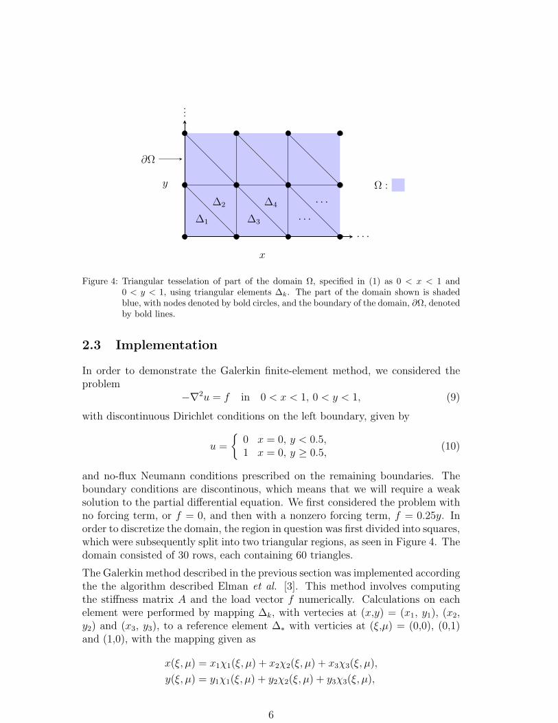
Figure 4: Triangular tesselation of part of the domain Ω, specified in (1) as 0 < x < 1 and0 < y < 1, using triangular elements ∆k. The part of the domain shown is shadedblue, with nodes denoted by bold circles, and the boundary of the domain, ∂Ω, denotedby bold lines.

2.3 Implementation

In order to demonstrate the Galerkin finite-element method, we considered theproblem

−∇2u = f in 0 < x < 1, 0 < y < 1, (9)

with discontinuous Dirichlet conditions on the left boundary, given by

u =

0 x = 0, y < 0.5,1 x = 0, y ≥ 0.5,

(10)

and no-flux Neumann conditions prescribed on the remaining boundaries. Theboundary conditions are discontinous, which means that we will require a weaksolution to the partial differential equation. We first considered the problem withno forcing term, or f = 0, and then with a nonzero forcing term, f = 0.25y. Inorder to discretize the domain, the region in question was first divided into squares,which were subsequently split into two triangular regions, as seen in Figure 4. Thedomain consisted of 30 rows, each containing 60 triangles.

The Galerkin method described in the previous section was implemented accordingthe the algorithm described Elman et al. [3]. This method involves computingthe stiffness matrix A and the load vector f numerically. Calculations on eachelement were performed by mapping ∆k, with vertecies at (x,y) = (x1, y1), (x2,y2) and (x3, y3), to a reference element ∆∗ with verticies at (ξ,µ) = (0,0), (0,1)and (1,0), with the mapping given as

x(ξ, µ) = x1χ1(ξ, µ) + x2χ2(ξ, µ) + x3χ3(ξ, µ),

y(ξ, µ) = y1χ1(ξ, µ) + y2χ2(ξ, µ) + y3χ3(ξ, µ),

6

(a) f = 0 (b) f = 0.25y

Figure 5: Solution to the spatial problem described in (1) with boundary conditions given in(10) along x = 0 and no-flux conditions on the remaining boundaries, with (a) f = 0and (b) f = 0.25y.

with

χ1 = 1− ξ − µ,χ2 = ξ,

χ3 = µ.

This simplified the numerical evaluation of the integrals within the definition ofA and f . Integrals performed over an element were performed using triangularquadrature such that ∫

∆∗

h(ξ, µ) dξ dµ ≈ 1

2h(1/3, 1/3),

while the trapezium rule was applied in order to evaluate line integrals along theedges of elements. The stiffness matrix and load vector were then assembled andmapped back into the (x,y) domain. The solution u to the equation Au = f wasthen computed using MATLAB. The results may be seen in Figure 2.3.

We see that in both cases, the heat flows into the domain where the boundaryis equal to one, and out of the domain where the boundary is equal to zero. Inthe figure with a forcing term, we see that the gradient of the heat flow is steeperin the bottom half of the domain and less steep at the top of the domain, as thecontribution from the forcing term is proportional to y. It is important to notethat the discontinuous boundary condition does not pose a problem in either case,due to the nature of numerical finite-element methods.

3 Finite-Element Methods on a Time-Varying

Problem

We may now extend the ideas developed in the previous section in order to developa scheme for solving the time-varying problem given in (3, 4). To accomplish this,

7

we obtain a weak formulation for the solution in space, and approximate the solu-tion in space by finite elements as before. This will produce a system of ordinarydifferential equations which may be solved using finite difference methods. Wewill use the Euler method, although other methods are applicable.

3.1 Weak formulation and Finite Element Scheme

The weak formulation for the time-varying problem given in (3) takes the form∫Ω

∂u

∂tw +

∫Ω

∇u ·∇w =

∫Ω

wf +

∫∂Ω

wgN .

We then discretise the spatial domain as before, and apply the Galerkin approxi-mation such that we search for uh ∈ H1

E that solves the equation in a finite sub-space, given by S0 = spanφ1, φ2, . . . , φn. We therefore find that the Galerkinequation takes the form∫

Ω

∂uh

∂tw +

∫Ω

∇uh ·∇w =

∫Ω

wf +

∫∂Ω

wgN . (11)

Aside from the time-derivative, this equation is identical to that given in (7). Assuch, each of these terms has been addressed in the previous section. It remainsto be demonstrated how the time-derivative alters the resulting system. In orderto discretise this term in space, we begin with the expression for uh given in (6).From this, we see that

∂uh

∂t(x, t) =

n∑j=1

duj

dt(t)φj(x) +

n+n∂∑j=n+1

duj

dt(t)φj(x) ∈ H1

E.

We therefore find that the discrete equation contains∫Ω

∂uh

∂tw =

n∑j=1

duj

dt(t)

∫Ω

φj(x)φi(x) +

n+n∂∑j=n+1

duj

dt(t)

∫Ω

φj(x)φi(x).

The time-varying discretised system may therefore be expressed using (6) as

n∑j=1

uj

∫Ω

φjφi +n∑

j=1

uj(t)

∫Ω

∇φj · ∇φi =

∫Ω

fφi +

∫∂ΩN

φigN −n+n∂∑j=n+1

uj

∫Ω

∇φj · ∇φi −n+n∂∑j=n+1

uj

∫Ω

φjφi.

This is a linear system of semi-discrete first-order ordinary differential equationsof the form Mu(t) + Au(t) = f, with A defined in (8), M is given by

M = mi,j where mi,j =

∫Ω

φjφi,

8

and f = (f1, f2, . . . , fn)T takes the new form

fi =

∫Ω

fφi +

∫∂ΩN

φigN −n+n∂∑j=n+1

uj

∫Ω

∇φj · ∇φi −n+n∂∑j=n+1

uj

∫Ω

φjφi.

3.2 Euler Method

We now use the Euler method [2] in order to write the semi-discrete system givenby Mu(t) + Au(t) = f as a fully discretised system. If we write

uk = (u1(k∆t), u2(k∆t), . . . , un(k∆t))T ,

for k = 1, 2, . . ., the Euler method involves approximating the time-derivatives as

u(k∆t) ≈ uk+1 − uk

∆t.

The semi-discrete system at some t = k∆t therefore becomes

M(uk+1 − uk) + ∆tAuk = ∆tf,

with some prescribed initial condition u0. As such, we can solve a linear systemat each time-step given by

Muk+1 = (M −∆tA)uk + ∆f, (12)

where u0 is known, and each subsequent uk may be obtained from uk−1. Assuch, we may now obtain the solution for the system over a number of time-steps by solving the fully-discretised linear system at each time step (that is, fork = 1, 2, . . .).

It is possible to show that this method will be unstable for large enough ∆t,and therefore care must be taken when determining the time-steps that are tobe chosen when solving a problem. If the time-steps are too large, the solutionvectors will tend to infinity as k → ∞, even if the solution does not behave inthis manner.

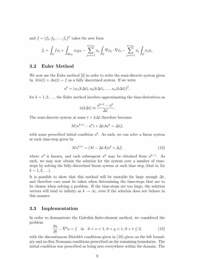
3.3 Implementation

In order to demonstrate the Galerkin finite-element method, we considered theproblem

∂u

∂t−∇2u = f in 0 < x < 1, 0 < y < 1, 0 < t ≤ 2, (13)

with the discontinuous Dirichlet conditions given in (10) given on the left bound-ary and no-flux Neumann conditions prescribed on the remaining boundaries. Theinitial condition was prescribed as being zero everywhere within the domain. The

9

discretization and finite-element scheme was identical to that applied to the sta-tionary problem, with the exception that the domain was divided into 18 rows,each containing 36 triangles, in order to improve the speed of computation.

The introduction of the time-stepping procedure as described earlier led to insta-bilities unless the time-steps were set to be extremely small. In order to ensurestability, the time-steps were chosen as ∆t = 10−5, although this could be madelarger without a loss of stability in the solution. The linear system described in(12) was solved at each time-step in order to demonstrate the behaviour of thesystem when flow starts at t = 0. Some of the results may be seen in Figure 3.3.We see that the flow tends towards the steady solution over time, as required.

Additionally, we could easily apply this method to more complicated problems,such as a problem with time-varying forcing terms or boundary conditions. Wecould also adapt the method to other governing equations by obtaining a differentweak formulation, as described in the previous section.

4 Conclusions

There are many partial differential equations that arise in applied mathematicsfor which no classical solution exists. In these cases, we must search for weaksolutions to the partial differential equations by expressing the equation in varia-tional form, which may be solved in order to obtain weak solutions to the originalproblem. We may use finite element methods in order to compute the solution tothe equations in variational form and subsequently obtain weak solutions to theoriginal equation.

The method of finite elements involved discretising the domain of the problem intoa set of elements, and defining a set of piecewise basis functions on these elementsin order to obtain an approximation space, generated by the basis functions. Itwas within this approximation space that the weak solution was sought. We sub-sequently applied the Galerkin finite element method which entailed constructinga stiffness matrix and load vector in order to express the finite element solutionas the solution to a linear system of equations, which could be solved numerically.This method was applied in order to solve two simple problems; the heat equationwithout a forcing term in the original equation, the same equation with a forcingterm included.

In order to solve time-varying problems, we obtained a variational form for theequation with a time-derivative included, and applied the finite element methodas before, obtaining a semi-discrete system that was discrete in space but continu-ous in time. This, however, resulted in a system of ordinary differential equations,rather than a fully discrete linear system. To fully discretise the system, we usedthe Euler method to discretise the ordinary differential equations in time. The re-sultant system was then solved using standard methods for solving linear systems.This method was applied in order to solve the time-varying heat equation and it

10

(a) t = 0 (b) t = 0.4

(c) t = 0.8 (d) t = 1.2

(e) t = 1.6 (f) t = 2

Figure 6: Solution to the time-dependent spatial problem described in (13) with boundary con-ditions given in 10 along x = 0 and no-flux conditions on the remaining boundaries,with u = 0 initially within the domain. The solutions is shown at regular intervalsbetween t = 0 and t = 2.

11

was observed that the computed solution evolved from the initial configurationtowards the steady solution as time progressed.

A number of extensions to the methods described here were touched upon. We canconsider a range of different equations, however doing so involves determining thevariational form for each new equation. It is possible to use elements of differentshapes, such as quadrilateral elements. Additionally, it is possible to considerhigher-order piecewise basis functions, such as quadratic or cubic basis functions.In many cases, these can give greater accuracy, but require more nodes withineach element, increasing computational cost. We could also consider differentmethods of discretisation in time, such as Runge-Kutta methods, and apply thecurrent scheme to more demanding time-varying problems, such as problems withtime-varying boundary conditions or forcing terms.

A Example finite-element solver

This code was used to discretise the system in question and apply the Galerkinfinite-element method used on a simple linear basis with triangular elements inorder to solve the system. This code was used to produce the results in the report,with minor modifications depending on the problem in question.

1 clear all2

3 % Discretisation of domain4 T = 10; % Triangles per row (even)5 N = T/2 + 1; % Nodes per row6 rows = 5; % Number of rows7 Xt = linspace(0,1,N); % Range in x8 Yt = linspace(0,1,rows+1); % Range in y9 X = [];

10 Y = [];11 for i = 1:rows+112 X = [X Xt];13 Y((i-1)*N+1:i*N) = Yt(i)*ones(1,N);14 end15 nodes = length(X); % Number of nodes in system16 triangles = T*rows; % Number of elements in system17

18 L = Xt(2)-Xt(1); % Distance between nodes19 Jk = Lˆ2; % Twice the area of each element20

21 % Contiguous list of nodes on boundary22 B = [1:N:(rows-1)*N+1 rows*N+1:(rows+1)*N ...23 rows*N:-N:N N-1:-1:2];24

25 % Forming Connectivity Matrix C26 C = zeros(4,triangles);27 C(1,:) = 1:triangles;

12

28 for i = 1:rows29 C(2,(i-1)*T+1:i*T) = ceil(C(1,1:T)/2)+(i-1)*N;30 end31 C(3,1:2:triangles-1) = C(2,1:2:triangles-1)+N;32 C(3,2:2:triangles) = C(2,1:2:triangles)+1;33 C(4,:) = C(2,:)+N+1;34

35 % Forming Stiffness Matrix A and Load Vector f36 dchidxi = [-1 1 0]; % Partial derivatives37 dchidnu = [-1 0 1];38 Jstar = 0.5; % Size of reference element39

40 for k = 1:triangles41

42 % Finding spatial coordinates of vertices43 X1 = X(C(2,k));44 X2 = X(C(3,k));45 X3 = X(C(4,k));46 XX = [X1 X2 X2];47 Y1 = Y(C(2,k));48 Y2 = Y(C(3,k));49 Y3 = Y(C(4,k));50 YY = [Y1 Y2 Y3];51 CC = [C(2,k) C(3,k) C(4,k)];52

53

54 for i = 1:355 for j = 1:356 Aloc(i,j,k) = ((Y3-Y1) * dchidxi(i) + ...57 (Y1-Y2) * dchidnu(i)) * ...58 ((Y3-Y1) * dchidxi(j) + ...59 (Y1-Y2) * dchidnu(j)) * ...60 Jstar/Jk + ((X1-X3)*dchidxi(i) + ...61 (X2-X1) * dchidnu(i)) * ...62 ((X1-X3) * dchidxi(j) + ...63 (X2-X1)*dchidnu(j)) * Jstar/Jk;64 end65

66 xstore = 0;67 ystore = 0;68 for j = 1:369 xstore = xstore + XX(j)/3;70 ystore = ystore + YY(j)/3;71 end72 % Define the function f as ffunc(x,y)73 floc(k,i) = 0.5*ffunc(xstore, ystore)*2*Jk/3;74

75 if sum(CC(i) == B) > 076 floc(k,i) = floc(k,i) + L/2*GN(XX(i),YY(i));77 end78

79 end80 end81

13

82 Pt = C(2:end,:);83 P = Pt';84

85 A = zeros(nodes,nodes);86 f = zeros(nodes,1);87 for k = 1:triangles88 for j = 1:389 for i = 1:390 A(P(k,i),P(k,j)) = A(P(k,i),P(k,j)) + Aloc(i,j,k);91 end92 f(P(k,j)) = f(P(k,j)) + floc(k,j);93 end94 end95

96 UJ = linspace(0,1,rows+1);97

98 % Setting Dirichlet condition edge of domain.99 for i = 1:rows+1

100 A(N*(i-1)+1,:) = zeros(1,nodes);101 A(N*(i-1)+1,N*(i-1)+1) = 1;102 end103

104 % Obtaining the steady-state solution105 uout = A\f;106 umapss = reshape(uout, T/2+1, rows+1);107 umapss = umapss';108

109

110 % Computing Mass Matrix M111 for k = 1:triangles112 for i = 1:3113 for j = 1:3114 Mloc(i,j,k) = 0.5*(1/3)*(1/3)*Jk;115 end116 end117 end118 M = zeros(nodes,nodes);119 for k = 1:triangles120 for j = 1:3121 for i = 1:3122 M(P(k,i),P(k,j)) = M(P(k,i),P(k,j)) + Mloc(i,j,k);123 end124 end125 end126

127 % Setting timesteps128 dt = 0.000001;129 Nsteps = 100000;130 usol = zeros(length(f), Nsteps/10000);131 uk = zeros(length(f),1);132

133 % Applying Dirichlet conditions134 for i = 1:rows+1135 M(N*(i-1)+1,:) = zeros(1,nodes);

14

136 M(N*(i-1)+1,N*(i-1)+1) = 1;137 end138

139 for i = 2:Nsteps140

141 % Creating load vector142 fnew = (M - dt*A)*uk + dt*f;143

144 % Performing Euler step145 for k = 1:rows+1146 fnew(N*(k-1)+1) = round(UJ(k));147 end148 uk = M\fnew;149

150 % Storing solution151 if i/10000 == round(i/10000)152 usol(:,i/10000) = uk;153 end154 end155

156 % Preparing solution for visualisation157 umap = reshape(usol(:,end), T/2+1, rows+1);158 umap = umap';

References

[1] W F Ames. Numerical Methods for Partial Differential Equations. AcademicPress, New York, 1992.

[2] B Carnahan, H A Luther, and J O Wilkes. Applied Numerical Methods. JohnWiley and Sons, New York, 1969.

[3] H Elman, D Silvester, and A Watham. Finite Elements and Fast IterativeSolvers. Oxford University Press, Oxford, 2005.

[4] J Ockendon, S Howison, A Lacey, and A Movchan. Applied Partial DifferentialEquations. Oxford University Press, Oxford, 2003.

[5] Q A Press, B P Flannery, S A Teukolsky, and W T Vetterling. Numericalrecipes: The Art of Scientific Computing. Cambridge University Press, NewYork, 1986.

15