Finite Element Modeling in Musculoskeletal Biomechanics · 2004-10-20 · Finite Element Modeling in Musculoskeletal Biomechanics ... by means of finite element analysis, has proven

Brown336

336

JOURNAL OF APPLIED BIOMECHANICS, 2004, 20, 336-366© 2004 Human Kinetics Publishers, Inc.

ORIGINAL RESEARCH

Thomas D. Brown is with the Orthopaedic Biomechanics Laboratory, 2181 Westlawn,University of Iowa, Iowa City, IA 52242.

Finite Element Modeling inMusculoskeletal Biomechanics

Thomas D. BrownUniversity of Iowa

Numerical approximation of the solutions to continuum mechanics boundaryvalue problems, by means of finite element analysis, has proven to be of incal-culable benefit to the field of musculoskeletal biomechanics. This article brieflyoutlines the conceptual basis of finite element analysis and discusses a num-ber of the key technical considerations involved, specifically from the stand-point of effective modeling of musculoskeletal structures. The process ofconceiving, developing, validating, parametrically exercising, and interpret-ing the results of musculoskeletal finite element models is described. Perti-nent case study examples are presented from two series of finite element models,one involving total hip implant dislocation and the other involving femoralhead osteonecrosis.

Key Words: stress analysis, computations, tissue mechanics

Transmission of mechanical load is a salient function of musculoskeletaltissues, organs, and prostheses. Purposeful musculoskeletal activity depends bothon local availability of the necessary mechanical impetus and on capability of theinvolved tissues/ organs/ implants to sustain the necessary loads without undergo-ing structural failure. Functionally, structural failure can take one of several forms.There can be direct irreversible degradation of mechanical competence, such asfrom catastrophic rupture of a tendon, fatigue fracture of a bone, plastic yield of asurgical implant, etc. Or there can be deformations which, while reversible, are soexcessive (e.g., hyperlaxity of an articular joint) as to compromise neuromuscularcontrol, load actuation efficacy, or global structural stability. Alternatively, failurecan occur because of a biologically mediated cascade of events accompanyingdisruption of tissue homeostasis, due to the local mechanical milieu being outsideof physiologically appropriate limits. Examples of the latter include disuse os-teoporosis of a bone, or catabolic degradation of articular cartilage matrix bychondrocytes experiencing excessive geometric distortion. Successful transmis-sion of necessary mechanical actuation therefore depends on avoiding inappropri-ate intensity of mechanical loading. For that reason, ascertaining levels of localmechanical stress is one of the central problems of biomechanics.

Finite Element Modeling 337

Background/Historical Overview

Much of the archival literature in the field of engineering structural mechanics,prior to about the 1970s, dealt with using analytical mathematical techniques todetermine stress distributions in objects of engineering interest. The theoreticalbasis for determining mechanical stress in a continuous isotropic elastic mediumdates from Cauchy’s work in the 1820s (Sokolnikoff, 1956). This takes the form ofpartial differential equations for equilibrium (Equ. 1) and for geometrical compat-ibility (i.e., no void openings or material overlaps) (Equ. 2), subject to a set ofboundary conditions such as a prescribed traction force distribution (Equ. 3):

(1)

(2)

and (3)

Here, per indicial notation convention, the subscripts i, j, and k denote the respec-tive orthogonal directions, repeated subscripts denote summation over the rangeof 1 to 3, and subscripted commas designate partial differentiation. The symbol τdenotes stress, F designates the body force vector (whose components are Fi), ∇2 isthe Laplacian operator (∇2ϕ = ϕ,ii ), v is the Poisson ratio, Θ is the first stress in-variant (= τii ), δij is the Kroniker delta (δij = 1 if i = j, 0 otherwise), div is thedivergence operator (div A = Ai,i), ej are the direction cosines of the external sur-face normal e, and T is the (traction) stress vector acting at a surface site whoseexternal normal is e. Solving such sets of partial differential equations called for ahigh level of skill in applied mathematics, with many classes of stress analysisproblems involving extraordinary solution complexity. Even so, analytical solu-tions were generally able to address only objects of simple geometry, comprisingmaterials with relatively simple mechanical properties, subjected to relatively simpleloading conditions. Since biological systems are geometrically irregular, and sincethey generally have complicated distributions of material mechanical propertiesand are subject to complicated loadings, analytical solutions from classical me-chanics were seldom either feasible or meaningful for stress analysis problems inbiomechanics.

That situation has changed radically over the last three decades, due to theadvent of numerical approximation techniques, enabled by digital computation.Finite element analysis (FEA) has arguably been the flagship among these ap-proximation techniques. In FEA, the basic idea is that rather than obtaining anexact algebraic solution of the governing partial differential equations throughoutthe domain of interest, one instead numerically solves a system of simultaneousequations that arise from enforcing those governing equations for an array of dis-crete simplified subdomains (elements). Within these individual elements, spe-cific interpolation functions (usually polynomials) are assumed, from whichcontinuous internal variables (e.g., strains) are piecewise approximated on the ba-sis of corresponding parameters (e.g., displacements, in the case of strain) evalu-ated at a discrete number of characteristic local points (nodes).

This conceptual approach had its mathematical roots in Courant’s work inthe early 1940s (Bathe, 1996), with the first applications in physics (Synge, 1957)

–

–e

– ––

Brown338

and in engineering (Argyris & Kelsey, 1954) appearing in the mid-1950s. Coinageof the term “finite element analysis” is frequently attributed to R.W. Clough (1960),who used it in a civil engineering conference presentation in 1960. The ensuingdecade witnessed vigorous development both of the underlying theoretical basisand of its computational implementation, driven especially by analysts in the fieldsof structural mechanics and aeronautical engineering. Beyond its initial applica-tion to static structural problems, the FEA piecewise approximation approach provedapplicable to dynamic structural problems, to fluid mechanics, to thermal and masstransport analysis, and to electromagnetic field analysis and other continuum fieldproblems.

The Role of FEA in Biomechanics

The first applications of FEA to biomechanics, which appeared in 1972, involvedisotropic linearly elastic structural analyses of bone, performed by groups workingindependently in the U.S. (Rybicki et al., 1972) and in the Netherlands (Brekelmanset al., 1972). This new capability’s benefit to the field of biomechanics was imme-diately evident: For the first time, one could calculate mechanical stresses in bod-ies having complicated shapes, complicated material distributions, and/orcomplicated loadings. Other types of biomechanical complexity subsequently ad-dressed have included material anisotropy, material and geometrical nonlinearity,contact and interface nonlinearities, time-variant loadings, adaptive behavior (ma-terial and geometrical), and fluid/structure interactions. The FEA biomechanicsliterature now encompasses many hundreds of papers. Surveys of work of the first(Huiskes & Chao, 1983) and second (Huiskes & Hollister, 1993) decades in thisfield were necessarily restricted to reviewing just small subsets of the highlights.

The purpose of the present article is to discuss a number of considerationspertinent to applying FEA to research problems in biomechanics, especially inmusculoskeletal structural analysis. Didactic presentation of the formulative basisfor FEA, normally the subject of entire semester-long university courses at theadvanced engineering undergraduate or graduate level, is necessarily beyond thescope of this brief discussion.

Biomechanical FEA studies sometimes involve man-made geometries (e.g.,surgical implants), sometimes natural geometries (anatomical structures), and some-times both. For man-made geometries, mesh zonings at the simplest level can bebased on nominally corresponding geometrical abstractions. More typically nowa-days, they are user-built to approximate the physical objects at an appropriate levelof detail, or they are generated automatically or semi-automatically by utility rou-tines which translate the data in the computer aided engineering files used to actu-ally manufacture the part. Regarding natural geometries, a key consideration iswhether the anatomic representation is generic vs. case- (or patient-) specific. Sourcegeometric data for the meshing of natural structures nowadays usually come fromthree-dimensional imaging modalities such as computed axial tomography (CT),magnetic resonance imaging (MRI), or confocal microscopy. Sometimes photo-graphs of serial physical sections are used instead, and on rare occasions, planefilm or biplanar xrays. Geometric fidelity typically depends on the resolution ofthe pixel or voxel image source. Another consideration is that such image sourcesoften have limited capability for delineating subregions of differing material be-havior.


Finite element program libraries now incorporate a wide range of optionsfor material property representation, including linear and nonlinear elasticity, plas-ticity, hyperelasticity (rubber-like materials), viscoelasticity, poroelasticity, andbimodal behavior for tension vs. compression. Various types of material symmetryare readily accommodated, including isotropy, transverse isotropy, and orthotropy.Since material representation is normally specified in a piecewise manner, the pres-ence of material inhomogeneity presents no computational difficulty. Commonlyused treatments include regional homogeneity, element-specified properties, and(less frequently) element properties interpolated from node-specified properties.Computational treatments also are available for many commonly used compositearrangements. For practical purposes, the realism of material representation in bio-mechanical problems is far more frequently limited by available experimental datathan by algorithmic capabilities.

There are two primary sources of complexity in the loadings typically en-countered in biomechanical finite element studies. The first complexity is tempo-ral: Some systems are appropriately analyzed with a single static loading, othersystems with a series of different quasi-static loadings, yet other systems meritfully dynamic treatment (i.e., inertial effects included). Occasionally, modal analysisis invoked for applications such as vibration studies. The second source of com-plexity is the spatial distribution of loading. Point loadings (the simplest situation)are relatively rare, as are line loadings. Most frequently, loadings of interest occuracross surfaces, and most commonly they are nonuniformly distributed. These cantake the form of prescribed traction distributions, or they can be loading-contin-gent, as for example in contact problems.

Sometimes it is appropriate to also superimpose a distributed body force toaccount for weight. Besides loading, the other commonly encountered type of ex-ternal influence is displacement boundary conditions. These can take the form of aconstraint against motion in one or more degrees of freedom, either applied atindividual element nodes or along element edges or faces. Alternatively, ratherthan fixities, displacement boundary conditions can involve prescribed nonzerodisplacements in one or more degrees of freedom, again specified at nodes, alongelement edges, or over element faces. For some problems it is appropriate to makeprovision for mechanical interaction across an interface. One type of interfacetreatment is friction-dependent slip/nonslip. Another is gap closure: no tensiontransmission, but allowing for transmission of compression at sites of gap closure.Formal contact treatments can include shear as well as compression, and in in-creasing order of complexity can involve sticky contact (no relative tangentialmotion of contact surfaces), small slip contact, or large displacement sliding con-tact. And, a number of specialty formulations have been developed to model othertypes of interface behavior.

Stages of the Modeling Process

Finite element studies generally involve five stages. The first stage is developmentof specialty coding, if appropriate to the problem at hand. (This step is now unnec-essary in most studies, which are well accommodated by the many features andcapabilities already incorporated in the major program packages available com-mercially.) The next phase, known as preprocessing, involves prescribing the meshgeometry, specifying the material property distributions, and designating the load-

Brown340

ing. Then the finite element solution is executed computationally, a process usu-ally involving little or no direct interaction with the user. There then follows astage known as postprocessing, where the FE solution’s raw output is used to com-pute variables of interest, and where selected information is displayed graphically.The final stage is that of interpretation of the results, a process heavily dependenton analyst judgment.

In research settings, these four (or five) stages typically proceed iteratively,over weeks or months, as different aspects of a model are brought into ever-betterconsonance with physical/clinical reality, and as issues influencing system behav-ior are explored in context. Computer CPU time to execute the actual finite ele-ment solutions (Stage 3) is usually just a small fraction of elapsed calendar time inan FE project, although models at the more complex end of the spectrum can some-times involve multihour, overnight, or even multiday solution runs.

The great majority of biomechanical finite element models utilize commer-cial software, both for pre- and postprocessing (e.g., PATRAN, SUPERTAB,FEMGEN, GIFTS) and for the actual solution phase (e.g., ABAQUS, ANSYS,NASTRAN, MARC, ADINA). These are all large program packages with exten-sive libraries of features from which the user can select. In recent years the majorFE solution programs have greatly improved their qualities and capabilities re-garding user interface, and thus have gained an increased marketplace share inpre- and postprocessing.

Elements and Nodal Forces

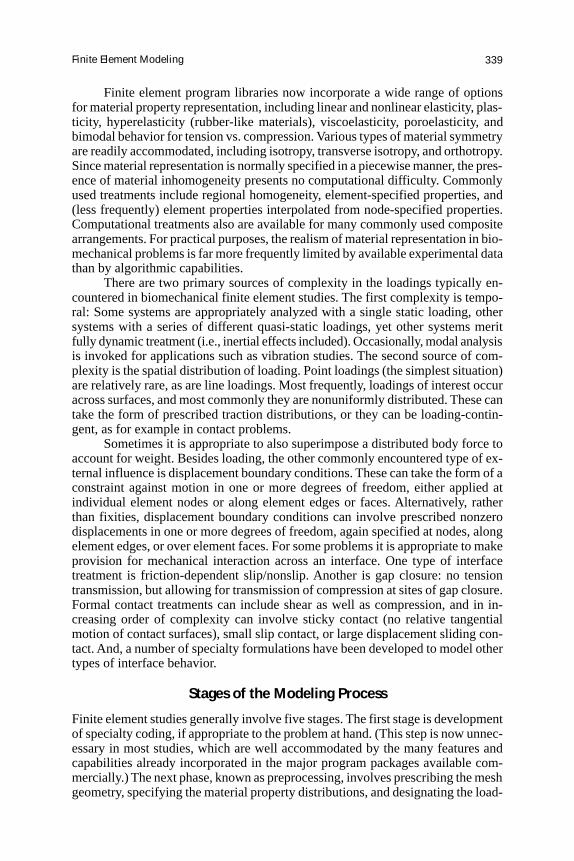
To appreciate why the field of finite element analysis is so intimately coupled withdigital computation, it is useful to understand how the finite element approach topiecewise discretization is implemented numerically. Here the situation of elasticstructural analysis, the simplest and most common of FE formulations, is illustra-tive. Consider the situation of a linear spring (Figure 1a), which can alternativelybe viewed as a one-dimensional finite element. Application of a force f causes thetwo ends of the spring (or nodes of the element) to displace a distance u, depend-ing on the stiffness k of the spring. Mathematically, this relationship is simply f =k·u. The two-dimensional counterpart (Figure 1b) is a quadrilateral element. Herethere are four nodes, each of whose displacements involves two variables (e.g., anx- and a y-component, in conventional Cartesian coordinates.) Hence the element’sdisplacement is characterized in terms of an eight-member nodal displacementvector, {u}. Similarly, each node can experience a distinct force, again involvingtwo components, so the system’s overall force can be expressed in terms of aneight-member nodal force vector {f}.

The set of nodal displacements resulting from a given set of nodal forces(Equation 1b) depends on the element stiffness, specified in terms of a two-dimen-sional array [k] known as the element’s stiffness matrix. Mathematically, analo-gous to the spring, this relationship is {f} = [k]·{u}. Taking this idea further, consideran assemblage of two-dimensional elements (Figure 1c). Most of the nodes in thissystem are shared by two or more elements, which provides a mechanism throughwhich the deformations of all elements are interlinked. Mathematically, again analo-gous to the spring, the global behavior of this system is conveniently described interms of the vector/matrix relationship {F} = [K]·{U}, where {F} is the globalforce vector (40 members, in this 20-node, two-dimensional system), {U} is the


Figure 1 — Elements and stiffnessmatrices. For a simple liner spring(1a), essentially a one-dimensionalelement, application of a force fcauses a displacement u, in inverseproportion to the spring stiffness,i.e., f = k·u. In the 2-D counterpart(1b), the set of nodal displacements{u} and forces {f} are interrelated inaccordance with a geometrically andmaterially dependent local stiffnessmatrix [k]: {f} = [k]·{u}. Similarconcepts apply in a multi-elementsystem (1c), where the forces {F} anddisplacements {U} of the nodes ofthe entire system are linked in termsof the relation {F} = [K]·{U}, wherethe global stiffness matrix [K] isconstructed on the basis ofindividual nodes’ associations withmultiple elements.

global displacement vector (again, 40 members), and [K] is a 40 3 40 array knownas the global stiffness matrix. For a given {F}, calculating the corresponding {U}requires solving a system of 40 equations with 40 unknowns.

The coefficients in the local stiffness matrix depend on two factors, one physi-cal and the other geometric. The physical factor is the mechanical behavior of thematerial which the element comprises. In two dimensions, this can be character-ized as a 3 3 3 coefficient array [D] linking local stress (a three-member vector,two of whose members are the in-plane normal stress components, and one is thein-plane shear component) and local strain (similarly, three components). The geo-metrical factor is a relationship—usually an interpolation polynomial—throughwhich the element’s local internal strain is assumed/defined to depend on nodaldisplacements: this also takes the form of a two-dimensional array [B]. The localstiffness matrix [k] is obtained by element-wide integration (Equation 2) of thekernel [B]T [D] [B], where the superscript T denotes transposition. Element-wideintegration involves an area integral in two dimensions, and analogously a volumeintegral in three dimensions.

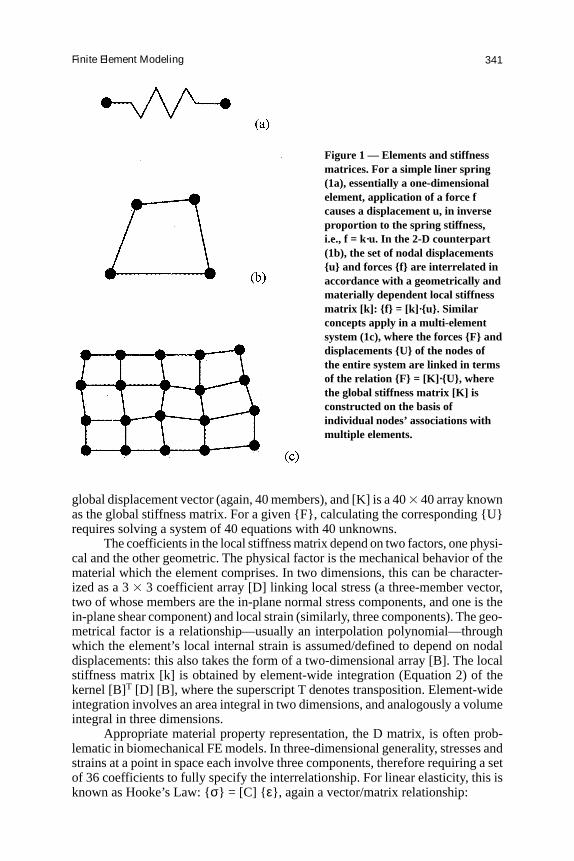
Appropriate material property representation, the D matrix, is often prob-lematic in biomechanical FE models. In three-dimensional generality, stresses andstrains at a point in space each involve three components, therefore requiring a setof 36 coefficients to fully specify the interrelationship. For linear elasticity, this isknown as Hooke’s Law: {σ} = [C] { ε}, again a vector/matrix relationship:

Brown342

Although the stiffness matrix is symmetrical about its main diagonal (i.e.,only 21 of the 36 members are unique), virtually never in biomechanics is this fullset of anisotropic material coefficients available. Instead, varying levels of simpli-fication are invoked, to fill out the array on the basis of limited available informa-tion. For example, Cowin and Sadegh (1991) have characterized cortical bone’sbehavior (units of GPa) as orthotropic:

Most nodes in a global structure are local nodes of multiple elements withinthat structure. Since mechanical equilibrium at these (shared) nodes therefore de-pends on the local stiffness matrices of all elements of which they are a part, thereis a basis for assembling all the local element stiffness matrices into a global stiff-ness matrix. Owing to the multiplicity of terms in the local element stiffness matri-ces, plus the large number of individual elements needed to discretize a complexglobal anatomic structure such as a bone, most contemporary finite element mod-els in biomechanics involve a very large global stiffness matrix, often with dimen-sions in the hundreds of thousands or more. One noteworthy recent model of anentire femur, zoned from micro-CT data, involved over 96 million three-dimen-sional elements (van Rietbergen et al., 2003). Fortunately for computation pur-poses, individual nodes are shared by elements only in a “nearby” neighborhoodof the overall global structure. If the nodes and elements are sequentially num-bered appropriately (built-in optimization routines for such purpose are now stan-dard in commercial FE programs and operate transparently to the user), globalstiffness matrices tend to be very sparse, with their nonzero terms clustered nearthe main diagonal.

This sparseness greatly facilitates specialized simultaneous equation pro-cessing algorithms that obtain solutions with orders of magnitude of fewer alge-braic operations (i.e., orders of magnitude more quickly) than “brute-force” matrixinversion. Even so, FE computations have always demanded high processor speed,large RAM, and large amounts of disk storage. Finite element analysis initiallywas exclusively the province of mainframe computers, but continued advances inplatform capabilities has enabled continued decentralization, first to high-endengineering workstations and nowadays routinely with PCs. Of course the larger

(4)

(5)


and faster the platform, the better. Powerful computers especially hold importantadvantages when working with nonlinear models, where the simultaneous equa-tion system solutions need to be obtained many times, rather than just once as isthe case in linear problems.

In structural problems, by far the most common class of FE formulationscurrently used in biomechanics, the base variable that emerges from equation sys-tem processing is the set of displacements of the nodes. (Recall, one is simplysolving for {U} from the equation {F} = [K] · {U}). Normally, however, informa-tion about site-specific point displacements in a structure is of limited practicalutility. Rather, one is usually interested in strains and/or stresses. To get that infor-mation from the base dataset, the global node displacements are referenced backto the corresponding local nodes of individual elements and the strain displace-ment ([B]) matrices of those elements, thus allowing evaluation of strain. Goingfurther, the strains are combined with the elements’ material coefficient ([C]) ma-trices, for evaluation of stress. Going still further, stresses and strains are typicallyused to evaluate yet other quantities of physical or physiological interest, such asprincipal stresses, strain energy density, von Mises equivalent stress, etc. In commer-cial programs, such postprocessing calculations normally are transparent to the user,who needs merely to select from an extensive menu of output data options.

Nonlinear Problems

The situation is complicated somewhat when structures undergo relatively largedeformations, such that deformation-dependent definitions of strain (e.g., Green-Lagrange strain) and stress (e.g., Cauchy stress) are necessary (Bathe, 1996), orwhen materials have deformation-dependent mechanical properties. Such nonlin-ear situations require that the finite element problem be solved incrementally. Toimplement this, a small fraction of the total load is initially applied, such that thestiffness matrix can be reasonably approximated based on the undeformed geom-etry, or the undeformed material properties, and a nodal displacement solutionobtained. The deformed nodal displacements are then used to update the geom-etry, or the material properties, at which point an updated stiffness matrix is calcu-lated, prior to application of an additional increment of the total applied loading,and so forth. Since the loading increments used for this purpose need to be rela-tively small, this vastly increases the computational effort compared to that re-quired for linear problems.

One of two major incremental solution strategies is utilized for nonlinearproblems. One of these is the explicit formulation, which is unconditionally stablenumerically, and which involves marching the process monotonically forward atprespecified increments which are sufficiently small that incremental adjustmentsof the nodal coordinates are not required to propagate through the structure atspeeds greater than the physically admissible (i.e., sonic) deformation wave veloc-ity. Alternatively, and more commonly, a conditionally and numerically stable im-plicit solution technique is employed, wherein a new solution is extrapolated fromthe previous increment, and nodal displacements are iteratively adjusted untilmechanical equilibrium is re-achieved within some specified tolerance limit. De-pending on the specifics of the situation, it may or may not be possible to implic-itly converge to a new equilibrium configuration for the increment size chosen. Ifnot, implicit solvers typically cut back the increment size and repeat the iterative

Brown344

procedure, recursively attempting to find a new equilibrium configuration involv-ing lesser extrapolation from the previous increment’s equilibrium solution, with asolution error abort condition being invoked if the increment size shrinks below aspecified threshold.

Zoning

In developing biomechanical FE models, arguably the most critical and challeng-ing aspect is zoning the physical structure into elements. Unless zoning is doneappropriately, reliable stress/strain data will not emerge. Many types and subtypesof elements are available in program libraries. The most commonly utilized ele-ment family, known as full continuum elements, imposes relationships betweenelement nodal forces and nodal displacements, in such a manner as to account forall stress and strain components present in the corresponding solid continuum.Some examples are shown in Figure 2. Depending on the number and positions oflocal nodes in an element, varying levels of accuracy and refinement can be achievedin approximating the spatial distribution of stresses and strains in the correspond-ing domain of the actual physical solid.

A key consideration in biomechanics is that using higher-order elements(i.e., those with more nodes than the number of vertices in the corresponding geo-metric solid) allows generating elements whose edges or faces are curved. Also, todeal with the geometrical transitions that are pervasive in many biological struc-tures, it is often convenient to specify that certain pairs (or even groups) of nodesin continuum elements remain coincident, thus “degenerating” the parent solid

Figure 2 — Typical 3-Delements. Higher-orderelements (which haveadditional nodes atlocations other than theelement vertices, such as atintermediate positionsalong edges or vertices) arecapable of more complexperformance, such asregistering heterogeneousdistributions of stress andstrain, and/or mappingonto curved boundaries ofthe object being meshed.


into a different type of solid having fewer vertices/ edges/ faces (Figure 3). Otherfamilies of elements are designed to offer economies of simplification, by notcomputing certain components of stress or strain for situations where those com-ponents either are negligible or are of no physical interest. Examples are truss andspring elements (Figure 4), beam elements (Figure 5), and shell elements (Figure6). Yet other families of elements implement special considerations that bear uponthe interrelationship of nodal forces and nodal displacement, such as contact ele-ments (Figure 7) or crack tip elements (Figure 8).

Two other concepts of element definitions merit mention, in light of fre-quent biomechanical implications. The first is local coordinates. Individual ele-ments are always specified in terms of their local nodes, which follow a specificnumbering sequence (Figure 9). The local node numbering sequence in turn pro-vides a basis for establishing local coordinate directions, specific to each element,and not necessarily coincident with global coordinate axes. Local coordinate di-rections are useful in biomechanics because they provide a basis for incorporatinglocal tissue structure, for example in terms of direction-dependent mechanical prop-erties (anisotropy), or in terms of stresses or strains relative to tissue planes. Corti-cal bone, for example, is approximately half again as stiff in the prevailing directionof its secondary osteons (e.g., longitudinally, in a diaphysis) than transversely, a

Figure 3 — Transition of element subdivisions in physical domains can be accomplishedusing “degenerative” elements, wherein multiple nodes of parent elements with a highernumber of surfaces are defined to be coincident. Transitions of this type are often helpfulwhen meshing geometrically complex biological structures.

Brown346

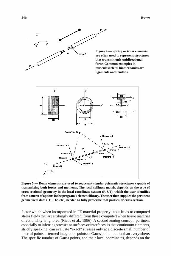
Figure 4 — Spring or truss elementsare often used to represent structuresthat transmit only unidirectionalforce. Common examples inmusculoskeletal biomechanics areligaments and tendons.

Figure 5 — Beam elements are used to represent slender prismatic structures capable oftransmitting both forces and moments. The local stiffness matrix depends on the type ofcross-sectional geometry in the local coordinate system (R,S,T), which the user identifiesfrom a menu of options in the program’s element library. The user then supplies the pertinentgeometrical data (H1, H2, etc.) needed to fully prescribe that particular cross-section.

factor which when incorporated in FE material property input leads to computedstress fields that are strikingly different from those computed when tissue materialdirectionality is ignored (Ricos et al., 1996). A second zoning concept, pertinentespecially to inferring stresses at surfaces or interfaces, is that continuum elements,strictly speaking, can evaluate “exact” stresses only at a discrete small number ofinternal points— termed integration points or Gauss point—rather than everywhere.The specific number of Gauss points, and their local coordinates, depends on the


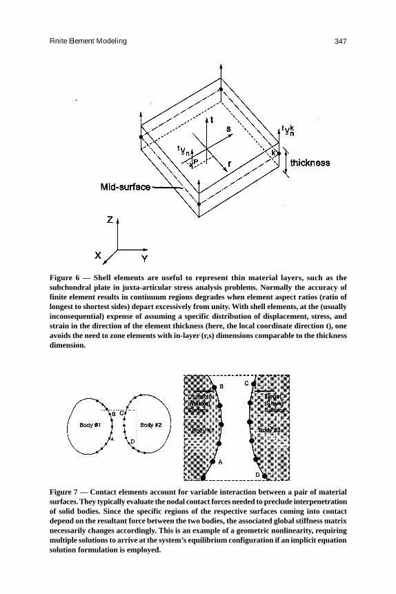
Figure 6 — Shell elements are useful to represent thin material layers, such as thesubchondral plate in juxta-articular stress analysis problems. Normally the accuracy offinite element results in continuum regions degrades when element aspect ratios (ratio oflongest to shortest sides) depart excessively from unity. With shell elements, at the (usuallyinconsequential) expense of assuming a specific distribution of displacement, stress, andstrain in the direction of the element thickness (here, the local coordinate direction t), oneavoids the need to zone elements with in-layer (r,s) dimensions comparable to the thicknessdimension.

Figure 7 — Contact elements account for variable interaction between a pair of materialsurfaces. They typically evaluate the nodal contact forces needed to preclude interpenetrationof solid bodies. Since the specific regions of the respective surfaces coming into contactdepend on the resultant force between the two bodies, the associated global stiffness matrixnecessarily changes accordingly. This is an example of a geometric nonlinearity, requiringmultiple solutions to arrive at the system’s equilibrium configuration if an implicit equationsolution formulation is employed.

Brown348

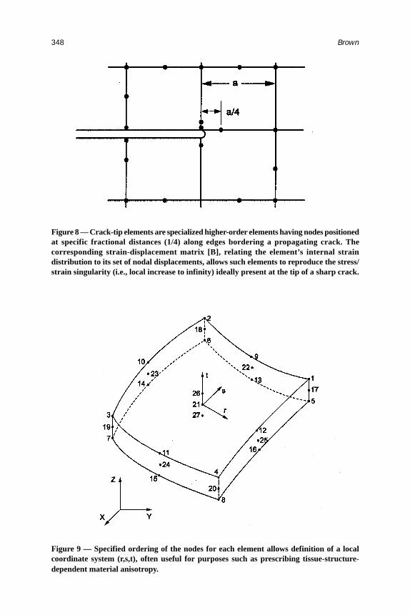
Figure 9 — Specified ordering of the nodes for each element allows definition of a localcoordinate system (r,s,t), often useful for purposes such as prescribing tissue-structure-dependent material anisotropy.

Figure 8 — Crack-tip elements are specialized higher-order elements having nodes positionedat specific fractional distances (1/4) along edges bordering a propagating crack. Thecorresponding strain-displacement matrix [B], relating the element’s internal straindistribution to its set of nodal displacements, allows such elements to reproduce the stress/strain singularity (i.e., local increase to infinity) ideally present at the tip of a sharp crack.


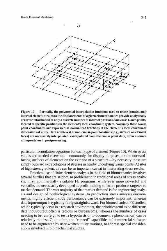
particular formulation equations for each type of element (Figure 10). When stressvalues are needed elsewhere—commonly, for display purposes, on the outward-facing surfaces of elements on the exterior of a structure—by necessity these aresimply outward extrapolations of stresses in nearby underlying Gauss points. At sitesof high stress gradient, this can be an important caveat in interpreting stress results.

Practical use of finite element analysis in the field of biomechanics involvesseveral hurdles that are seldom so problematic in traditional areas of stress analy-sis. First, commercially available FE programs, while ever more powerful andversatile, are necessarily developed as profit-making software products targeted tomarket demand. The vast majority of that market demand is for engineering analy-sis and design of nonbiological systems. In production stress analysis environ-ments, highly efficient code performance can be extremely important, whereasdata input/output is typically fairly straightforward. For biomechanical FE studies,which typically occur in a research environment, the priorities tend to be different:data input/output often is tedious or burdensome, whereas the numbers of casesneeding to be run (e.g., to test a hypothesis or to document a phenomenon) can berelatively modest. Quite often, the “canned” capabilities of commercial softwareneed to be augmented by user-written utility routines, to address special consider-ations involved in biomechanical studies.

Figure 10 — Formally, the polynomial interpolation functions used to relate (continuous)internal element strains to the displacements of a given element’s nodes provide analyticallyaccurate information at only a discrete number of internal positions, known as Gauss points,located at specific positions in the element’s local coordinate system. Normally these Gausspoint coordinates are expressed as normalized fractions of the element’s local coordinatedimensions of unity. Data of interest at non-Gauss-point locations (e.g., stresses on elementfaces) are necessarily interpolated/ extrapolated from the Gauss point data, often a sourceof imprecision in postprocessing.

Brown350

Specialty biomechanics augments unfortunately tend to be of little interestfrom a theoretical or numerical analysis perspective, and they tend to serve only avery small segment of the marketplace. FE users in the biomechanics communitytherefore share a stake in nurturing such developments wherever possible. An-other concern, also of a logistical nature, is that updates of commercial software,which tend to be market-driven, are rapid, relentless, and for practical purposesmandatory. The majority of that software market is in private industry, where or-ganizational cultures have evolved to provide their R&D component with the re-sources needed to remain competitive. Resource availability tends to be less inmost computational settings engaged in biomechanical modeling, such as univer-sities or health care research institutes.

Effective use of FEA in biomechanics also has several unique scientific con-siderations. First, the analyst should appreciate that individuals with a clinical orbiological background are often skeptical about the validity and utility of math-ematical models. Thus it is important to clearly justify why computed stresses helpanswer the question at hand. Where possible, avoidance of complicated param-eters or indices helps keep that basic message comprehensible and compelling tononspecialists. Input data (geometry, materials, loadings) should be based on asituation as closely related as possible to the problem at hand, and those data shouldbe as physically and biologically grounded as is practical. FE model developmentin new areas therefore often requires that the analyst be prepared, either directly orby collaboration, to collect specialty input data not available in the literature.

Geometry

Regarding geometry, three-dimensional models now constitute the norm. Aboutthe only appropriate uses of two-dimensional formulations are when the system ofinterest possesses approximate geometrical and material symmetry about a singleaxis (axisymmetric simplification), when it is a thin surface such as a membrane(two-dimensional plane stress), or when it is a cross-section of a long, prismaticstructure in which all sections can be assumed to behave comparably (two-dimen-sional plane strain). Two-dimensional idealizations also are appropriate, as an in-termediate stage of development, for formulations having an appreciable degreeof conceptual novelty. Otherwise, however, two-dimensional FE models appearrelatively infrequently in contemporary biomechanics research. Digitized imagesources are generally preferable, for purposes of accurately capturing the complexgeometry of biological constructs. Where possible, these should be coupled withobjective delineation of internal material boundaries or interfaces. Oftentimes, in-terpretation of computational results is facilitated by a graphic demonstrating FEmesh overlay onto the source geometry. One situation where idealized geometry isappropriate, however, is with man-made objects such as surgical implants; therethe best source of information is data from the CAE files used for the actual manu-facturing.

Material Properties

Because of biologic variability, biomechanical constructs almost always involvesome degree of idealization of material properties. Judgments in that regard arewithin the analyst’s legitimate purview, and can and should be made in a mannerthat facilitates the overall objectives of the analysis. Since material properties are


seldom unambiguously known in biomechanical FEA, it is usually a good practiceto conduct preliminary sensitivity trials, to gage solution sensitivity to plausiblevariations in the material input. This is particularly the case in nonlinear problems,where the “character” of the solution can vary appreciably, depending on whereone is operating in the state space of system parameters. Meshing should be donein such a manner that all distinct material regions are represented. In that regard,for a given problem size (i.e., for a given number of global nodes), low-orderelements having relatively few local nodes are normally preferable to high-orderelements for biomechanical models. The former provide better spatial resolutionfor delineating material property input, a consideration that usually far outweighsthe latter’s slight intrinsic numerical performance superiority.

Loadings

Loadings are another aspect of biomechanical FE models that usually call for ap-preciable judgment on the part of the analyst. Most living systems experience widefluctuations of loading during function, so it is usually desirable to input dutycycles that reflect this variation. For example, in studying stresses in a total hipprosthesis, it is desirable to consider a range of loadings that span those developedduring the gait cycle. Computationally, this is easy to do in linear problems, sincethe global stiffness matrix need not be recalculated; commercial FE packages nor-mally include an option for the user to specify multiple loading cases. Even innonlinear problems, however, the additional credibility provided by considering aphysiologically representative sequence of loadings normally more than justifiesthe extra time and expense involved. Most loadings in biomechanical systems aredistributed, rather than concentrated. Finite element codes provide a menu of op-tions for specifying those distributions. A commonly used choice is to specifyloadings individually for each element on the surface of a loaded structure. Fi-nally, in nonlinear problems, as with material property assumptions, it is usuallyprudent to evaluate solution sensitivity to loading assumptions, since model be-havior can be qualitatively very different in different regions of the parameter space.

Post-Processing

In reporting results from biomechanical FE models, the analyst needs to be cau-tious about reporting trends that are specific to individual components of stress orstrain. Different components of computed stress or strain can exhibit very differ-ent (sometimes even contradictory) responses to input variables. In that commonsituation, the analyst bears responsibility for choosing which, among many, outputvariable(s) merit attention, for purposes of characterizing the relevant aspects ofsystem behavior. Sometimes, conventional multicomponent indices (e.g., von Misesequivalent stress) available from FE postprocessing programs can be very helpfulin that regard, but their use should be limited to contexts in which the index hasdirect physical meaning. In other situations it may be appropriate to define andevaluate ad hoc multicomponent indices, a step normally requiring off-line calcu-lations using a separately written program (e.g., in FORTRAN or C++) or a spread-sheet.

In biomechanics, good graphics are key to a high-impact finite element model.In discussing stress distributions in a biomechanical construct, it is almost alwaysuseful to first give the reader/audience the “lay of the land” by presenting at least

Brown352

one full-field view of the structure being analyzed. Often a contour plot of thebaseline stress distribution works well for that purpose. However, to maximizetheir quantitative utility, contour plots require clearly identifiable gradations, andtheir scale annotations typically need to be enlarged from plotting program de-faults in order to be easily legible. Individual parametric influences are usuallybest illustrated by line plots, which afford space-economical demonstrations of theeffects of univariate, bivariate, or even trivariate input changes. Again, however,while most finite element postprocessing programs include basic line-plotting ca-pabilities, these often lack sufficient flexibility for use in biomechanical systems.Access to an adjunct imaging/ plotting/ analysis package is therefore highly desir-able to enable construction of ad hoc graphics.

Reliability and Validation

Since FEA is by nature an approximation technique, it is important to demonstratethat the results obtained are reliable. One consideration is to show that the mesh issufficiently refined that the solution will not change appreciably with additionalmesh refinement, i.e., that the numerical solution has converged mathematically.Two variants of convergence testing are typically used in the general field of finiteelement analysis, h-convergence and p-convergence (Figure 11). P-convergencetesting, which involves progressively higher order elements, is rarely performedin biomechanical models, because high-order elements are seldom appropriate,for reasons noted above. But even formal h-convergence tests are usually difficultto design in biomechanical modeling studies, since geometrically irregular struc-tures seldom lend themselves to systematic progressive refinements of zoning.Instead, what is often done is to perform an “informal” h-convergence test, involv-ing several alternative meshes with progressively increased resolution, but with-out the sort of uniformly systematic subdivisions that are practical for simplegeometric shapes.

Figure 11 — Successively refined spatial resolution can be achieved either by usingprogressively greater numbers of elements of the same order, or by progressively increasingthe order of a fixed number of elements. The former is far more common in biomechanics,owing to the typical need to account for material heterogeneity. Documenting that the levelof mesh refinement is such that the computed solution does not change appreciably foradditional refinement is the province of convergence testing. Doing this for element numbervs. element order is known as h- and p-convergence testing, respectively.


Another broad approach to demonstrating FE solution reliability is to per-form model validation. In order of increasing levels of model credibility provided,approaches to validation include:

1. Showing that the solution is reasonable and well-behaved, in the sense of beinginternally consistent;

2. Showing that the solution exhibits general consistency with existing literature;

3. Performing quantitative spot checks with existing literature;

4. Performing limit checks against available analytical solutions for related situa-tions;

5. Comparing FE results with directly corresponding prospective experiments.

Depending on the system being studied, various sources of information maybe appropriate for model validation. Surface strain measurements are one frequentlyused standard for comparison. Strain gages hold the advantage of giving directnumerical data. In biomechanical constructs, however, there can often be diffi-culty in making direct comparisons with FE, since the gage position and orienta-tion need to be precisely and unambiguously registered relative to the numericalmodel. This is especially problematic in the all-too-common situation where thesites of primary interest in the model have high gradients of strain. Photoelasticcoatings afford broader depiction of complex strain fields, but extracting specificnumerical values is difficult and tedious, and often yield data which are at bestonly approximate. Normally, therefore, photoelastic recordings are useful mainlyto confirm overall patterns in an FE-computed strain field.

An alternative basis for kinematic validation is to compare point-wise dis-placements or velocities. Sensors used for that purpose include both contactingmodalities such as linearly variable displacement transformers (LVDTs) and ex-tensometers, and noncontacting modalities such as eddy current transducers, ultra-sound, and laser position sensors. As with strain gages, however, the problem ofunambiguous spatial registration limits the available precision of comparisons.Finite element problems involving contact stress and/or fluid pressures are ame-nable to kinetic validation. Contact stresses can be measured statically with FujiFilm, or dynamically with sheet sensors such as TekScan® or EMed®. Fluid pres-sures can be measured using a wide variety of commercially available transducers.Yet another approach to physical validation is to compare (integral) process vari-ables, such as global accelerations or velocities of moving objects, flow rate offluids, weight loss in wear simulations, or other such summary variables pertinentto the problem at hand.

Interpretation

A final key component to successful use of finite element modeling in biomechan-ics is appropriate interpretation of the model’s results. Doing this effectively re-quires that the FE analyst have at least a working knowledge of the physical/ clinical/biological system under study. Since finite element models generate prodigiousamounts of output data, it is important to avoid information overload. Direct knowl-edge of the subject matter is invaluable for identifying the FE phenomena that aremost germane to the issues(s) under study. Subject knowledge also helps the ana-lyst avoid making observations that will appear trivial or irrelevant to experts in

Brown354

the field, and it helps the analyst identify contra-intuitive results that potentiallymerit reexamining the computational formulation or the input data. Subject knowl-edge also helps the analyst design parametric series that answer the question(s) athand with reasonable economy of effort, and it provides a basis for making criticalassessments of model limitations.

Interpreted in appropriate context, observations from biomechanical finiteelement models can be reported with a great deal of confidence and credibility.Numerical models are highly respected throughout the broad field of mechanics,and in many specialty areas their impact has been so pervasive as to displace ex-perimentation as the preferred means of inquiry. This is certainly not yet the casein biomechanics, but toward that end, one can realistically look forward to contin-ued dramatic improvements in the realism of biomechanical finite element models.

Examples

Case Study 1

Two sets of finite element case studies, drawn from recent research in the field oforthopaedic biomechanics, should serve to illustrate many of the above concepts.The first set of examples involves dislocation of total hip replacements. Here thegeneral goal of finite element modeling is to gain direct mechanistic insight intoways to reduce the incidence of this troublesome surgical complication. Clinicalregistry data in this area unfortunately have many confounding variables, and thushave proven capable of documenting relatively few statistically significant cause/effect relationships. Direct laboratory experimentation, primarily with cadavericmaterial, is expensive, unwieldy, and can address only a narrow range of paramet-ric influences and outcome measures.

For studying dislocations, the system of direct interest is the total hip im-plant, and the phenomenon of interest is disruption of normal ball-in-hemispheri-cal-socket articulation, due to impingement of the ball’s support base (termed theneck) against the rim of the socket. The proximate cause of impingement is exces-sive angular motion of the hip, which tends to be associated with various untowardpatient maneuvers, such as crossing one’s leg or rising from a low toilet seat. Theimpingement site serves as a fulcrum, about which the femoral head ball tends topivot, leading toward its being levered out of the socket.

Although geometrical idealizations were helpful in the exploratory phase ofFE model development, this was a situation where credibility of the results in theeyes of clinicians strongly depended on working with familiar, realistic implantgeometries. Therefore, the meshes (Figure 12) were zoned from CAE files (IGESfiles) used to manufacture the implants. A commercial pre-/postprocessing pro-gram (PATRAN) was used for that purpose. Since stresses in the metal femoralcomponent and in the metal shell backing of the socket (acetabulum) were not ofparticular interest, and since the elastic modulus of the metal in those memberswas orders of magnitude higher than that of the plastic socket (made of ultra-highmolecular weight polyethylene), the metal members were assumed rigid, afford-ing their representation purely by a surface mesh. The polyethylene was treated asan elasto-plastic solid, zoned into low-order wedge (5-face) and hexahedral (6-face) continuum elements. Socket meshing resolution was concentrated at the ex-pected impingement site, with suitable element density being inferred from h-typeconvergence testing (Figure 13). Because of expected stress concentrations at the


Figure 12 — Finite elementmesh used to study dislocationof total hip replacementimplants.

Figure 13 — Illustration of typical h-convergence testing, here undertaken to identify suitablemeshing density of a total hip acetabular component in the zones for which femoralcomponent neck impingement was feasible (30° zone) vs. nonfeasible (90° zone), respectively.These data showed that a problem size of at least 22,000 deg of freedom was necessary.

Brown356

impingement site, implying potentially large strains (up to 10s of %) for the poly-ethylene, finite deformation material nonlinearity was invoked.

The problem was simultaneously driven by two types of input, both experi-mentally grounded. Kinematically, a sequence of triaxial rotations was input forthe femoral component relative to the acetabular component, the latter’s outer (back-ing) shell surface being assumed to be rigidly fixed. Kinetically, a time-variantcontact force was input at the center of the femoral head, based on joint resultantcontact force calculated from an inverse dynamics multisegmental rigid body modelrun for (non-THA-implanted) individuals undergoing various motions known tobe associated with dislocations in THA patients. Motion data for dislocation-riskactivities were not previously available in the literature, and thus had to be cap-tured specifically for the intended finite element studies (Nadzadi et al., 2003).The finite element model, run using the ABAQUS program, then computed inter-nal and contact surface polyethylene stresses at each of typically 100 instants(frames) of discretized motion.

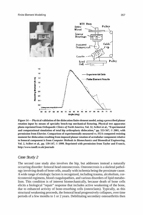
There were two outcome measures of primary interest: the range of motionprior to dislocation, and the peak moment developed to resist dislocation. Neitherof these are standard menu items in commercial finite element programs. For rangeof motion, it was necessary to define a physically meaningful criterion to desig-nate the exact instant of dislocation. The criterion used for that purpose was pas-sage of the resultant contact force off the hemispherical bearing surface. Thiscondition is associated physically with head escape from the socket, and was mani-fest computationally by the onset of numerical instability (i.e., Newtonian equilib-rium could no longer be achieved.) Regarding peak resulting moment, specialpurpose FORTRAN postprocessing code was written to summate the resultant ofall the individual moments (about the head center) of forces acting on externalsurface nodes of the polyethylene socket. The FE model was then experimentallyvalidated using a laboratory bench-top fixture designed to induce dislocation dueto imposed planar rotation of the acetabulum relative to the femur, and in whichresisting moment could be measured by a load cell. This imposed planar rotationconstituted a well-prescribed special case input sequence which could be unam-biguously replicated computationally (Figure 14).

Once developed and validated, this finite element model was used to para-metrically study dislocation propensity’s dependence on a wide range of influencefactors. Those factors included variations in specific attributes of implant design,of surgical positioning, and of patients’ hip joint motions. Such parametric datalend themselves well to presentation in line plot format, using various graphicsstructures (Figure 15). The upshot of such work has been the design of more dislo-cation-resistant implants (data from this model were used to assist in the design ofDePuy’s Pinnacle® Total Hip Section), the delineation of optimal orientations forsurgical implantation of THA components, and the identification of relative risksof various patient activities believed to be responsible for dislocations. Recent FEwork with THA dislocations (Figure 16) has involved embedding the implantcomponents in anatomically realistic bone structures, and representing the hipcapsule by means of hyperelastic elements whose input coefficients are set so as tomimic that tissue’s experimentally-observed stress/strain behavior (Stewart et al.,2004).


Case Study 2

The second case study also involves the hip, but addresses instead a naturallyoccurring disorder: femoral head osteonecrosis. Osteonecrosis is a skeletal pathol-ogy involving death of bone cells, usually with ischemia being the proximate cause.A wide range of etiologic factors is recognized, including trauma, alcoholism, cor-ticosteroid regimens, blood coagulopathies, and various disorders of lipid metabo-lism. This condition is of interest biomechanically, because death of bone cellselicits a biological “repair” response that includes active weakening of the bone,due to enhanced activity of bone-resorbing cells (osteoclasts). Typically, as thisstructural weakening proceeds, the femoral head progressively collapses, over timeperiods of a few months to 1 or 2 years. Debilitating secondary osteoarthritis then

Figure 14 — Physical validation of the dislocation finite element model, using a prescribed planarrotation input by means of specialty bench-top mechanical fixturing. Physical test apparatusphoto reprinted from Orthopaedic Clinics of North America, Vol. 32, Scifert et al., “Experimentaland computational simulation of total hip arthroplasty dislocation,” pp. 553-567, © 2001, withpermission from Elsevier. Comparison of experimentally measured vs. FEA-computed resistingmoment for dislocation resulting from imposed planar rotation of acetabular component relativeto femoral component is from Computer Methods in Biomechanics and Biomedical Engineering,Vol. 2, Scifert et al., pp. 139-147, © 1999. Reprinted with permission from Taylor and Francis,http://www.tandf.co.uk/journals

Brown358

Figure 15 — Results from parametric exercise of the dislocation finite element model. Inthis series the ability of the total hip implant to resist dislocation was assessed for motioninputs characteristic of leg crossing in an erectly seated position, for a total hip acetabularcomponent implanted at 20° of anteversion (i.e., rotation in the transverse plane), for variousangles of abduction (tilt in the coronal plane) ranging from 30° to 70°. The ability to conductsuch tests to isolate the effects of a single variable (here, acetabular component abduction)on an outcome measure of interest (here, peak resisting moment) is a major attraction offinite element analysis.

Figure 16 — Incorporation of capsule restraint and anatomic bony bed encasement in a3-D contact finite element analysis of total hip dislocation. In this formulation, the capsuleis characterized as a formal 3-D materially nonlinear region capable of arbitrary wrap-around contact with both the implant and the bony members. The locus of anatomic capsuleattachment on the respective bony members is depicted by the thick solid lines.


develops, due to the resulting articular surface incongruity. The only recourse at thatpoint is total hip replacement. Unfortunately, osteonecrosis patients tend to be youngand active, and they have an extremely high incidence of prosthesis loosening.

Osteonecrosis in the U.S. accounts for about 10% of the total hip patientpopulation, and for about 20% of that procedure’s aggregate societal cost. For thisreason there is great interest in finding ways to forestall structural collapse of thenatural femoral head. Finite element modeling has a role to play in that regard,since it provides a basis for assessing which aspects of disease involvement influ-ence the speed and severity of collapse, and it allows quantifying the degree ofimprovement of the adverse biomechanical environment afforded by structurally-motivated surgical interventions.

Meshing in this instance requires an anatomic image source. Four modali-ties have played a role in providing source data for that purpose: serial physicalsectioning, computerized tomography (CT) imaging, plane film radiographs, andmagnetic resonance (MR) imaging. Physical sectioning affords the highest spatialresolution, at least in the specific sections photographed, but the sectioning proce-dure is cumbersome, and being destructive, it obviously is applicable only to ca-daver specimens. CT scans hold the advantages of being available nondestructively,plus providing relatively good spatial resolution (voxel edge dimensions of typi-cally 1 mm or so) for contemporary images of whole major articular joints.

Another attraction of CT images for FEA of bone is that, besides geometry,the voxel source data are in the form of Hounsfield numbers, an index of localradio-density, and therefore are convertible, usually by linear regression (Ciarelliet al., 1991), to physical density and hence elastic modulus. In the case of FEmodeling of osteonecrosis, an idiosyncratic situation where the size, shape, andposition of the necrotic lesion are key determinants of collapse propensity, obvi-ously it is important to delineate the zone of involvement. MR scans are invaluablefor that purpose, since one of the early aspects of the pathogenesis is saponifica-tion of the marrow of the involved cancellous bone region, for which the changesin water content lead to characteristic changes in MR signal intensity. MR is sosensitive for that purpose that it has become the clinical standard when osteone-crosis is suspected. This is both good and bad for purposes of FE modeling. Sincethe information provided by MR is so definitive for diagnosis, CT scans are gener-ally not indicated clinically for these patients.

Conventional clinical MR sequences unfortunately do not perform well fordepicting cortical bone, so the best information available for osseous geometry isusually just plane film radiographs. A hybrid approach has therefore evolved forconstructing FE meshes for studying osteonecrosis: a generic density distributiontemplate for a normal proximal femur based on CT data, scaled appropriately onthe basis of patient-specific x-rays, and with the patient’s area of lesion involve-ment measured from MR images. Source data for material property attenuations innecrotic lesions have had to come from physical compression testing of samples(5-mm cubes) excised from pathology specimens (Brown et al., 1981).

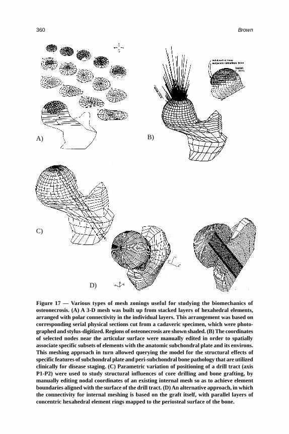
Different mesh zoning strategies have proven appropriate for different pur-poses of FE modeling of osteonecrosis. One approach, for sensitivity studies ex-ploring generic influences of lesion size/ shape/ location, has been to subdivide theproximal femur into serial transverse slabs, each such layer being further subdi-vided into concentric rings of (primarily hexahedral) elements (Figure 17a). Then,by considering specific subsets of these fixed elements to undergo material prop-

Brown360

C)

D)

Figure 17 — Various types of mesh zonings useful for studying the biomechanics ofosteonecrosis. (A) A 3-D mesh was built up from stacked layers of hexahedral elements,arranged with polar connectivity in the individual layers. This arrangement was based oncorresponding serial physical sections cut from a cadaveric specimen, which were photo-graphed and stylus-digitized. Regions of osteonecrosis are shown shaded. (B) The coordinatesof selected nodes near the articular surface were manually edited in order to spatiallyassociate specific subsets of elements with the anatomic subchondral plate and its environs.This meshing approach in turn allowed querying the model for the structural effects ofspecific features of subchondral plate and peri-subchondral bone pathology that are utilizedclinically for disease staging. (C) Parametric variation of positioning of a drill tract (axisP1-P2) were used to study structural influences of core drilling and bone grafting, bymanually editing nodal coordinates of an existing internal mesh so as to achieve elementboundaries aligned with the surface of the drill tract. (D) An alternative approach, in whichthe connectivity for internal meshing is based on the graft itself, with parallel layers ofconcentric hexahedral element rings mapped to the periosteal surface of the bone.

A) B)


erty attenuations representative of osteonecrosis, it is possible to systematicallysurvey the effects of individual characteristic parameters. Another meshing ap-proach, useful for investigating juxta-articular load transmission implications ofsubchondral plate involvement and (pathognomic) subchondral fracture, has beento adopt an ad hoc tangential element layering structure, with very high spatialresolution periarticularly, and much lower resolution elsewhere (Figure 17b).

A third approach, used to investigate the mechanical implications of thera-peutic core drilling and/or structural bone grafting, has been to manually edit thenodal coordinates of a preexisting serial-transverse-plane meshing structure, so asto align element boundaries with the material discontinuities introduced by thesurgery (Figure 17c). This strategy allowed systematic study of core/graft posi-tioning variants, in the interest of providing objective, mechanically-groundedsurgical guidelines. Of course, manual editing of preexisting 3-d FE meshes is alabor-intensive endeavor, and also has limited generality for studying surgical in-terventions such as bone grafts or implants, since oblique intersections betweenmesh planes and surgically-induced material discontinuities can sometimes leadto highly elongated or highly oblique elements, which are known to perform poorly.(Most commercial FE programs have report flags that warn the user when aspectratios of zoned elements exceed generally accepted thresholds. Often the prepro-cessing algorithms of these programs treat excessive violations of those good-practice norms as a formal error, explicitly terminating program execution.)

An alternative approach is intervention-based meshing, where characteristicgeometric features of the induced material discontinuity, rather than of the undis-turbed original anatomy, are used as the basis for structuring the mesh. An ex-ample is graft-based meshing to study fibular grafting (Figure 17d). Here the meshconsists of serial layers of concentric elements, but the element layering is perpen-dicular to the axis of the graft. This allows concentric element rings in each layer,with element boundaries aligned with the interface between the graft and the hostbone. Each such graft-based element layer terminates peripherally at its boundingplanes’ intersections with anatomic periosteal surface, the detection of which re-quired special preprocessing interpolation logic. Major commercially availablepreprocessing programs (PATRAN in this instance) include capabilities for theuser to write special command-language instruction sequences, to implement math-ematical operations of various sorts as part of the process of automated and/orinteractive mesh generation.

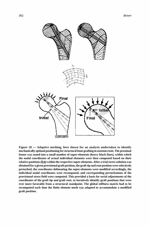
Another approach to meshing also merits mention: known as adaptive mesh-ing, it involves solution-contingent alteration of the geometry (and/or, more gen-erally, also of the material property distribution) during evolution of a multistageFE simulation. As applied to osteonecrosis, an example has been the use of struc-tural optimization analysis, to find the particular orientation and positioning of abone graft that provides the best possible load protection for a given lesion. This isimplemented (Figure 18) by subsectioning the structure into a small number ofsuper-elements having generic interconnection patterns (i.e., shared nodes on thesuper-element boundaries), but within which the coordinates of individual ele-ments can be conditionally changed.

Starting from a plausible “trial” position of the graft, positioning is system-atically perturbed (requiring corresponding nodal position changes, and stiffnessmatrix recomputation) to find which positioning change offers the best incremen-tal benefit in terms of reducing lesion stresses. This provides a basis for ever more

Brown362

Figure 18 — Adaptive meshing, here shown for an analysis undertaken to identifymechanically optimal positioning for structural bone grafting in osteonecrosis. The proximalfemur was zoned into a small number of super-elements (heavy black lines), within whichthe nodal coordinates of actual individual elements were then computed based on theirrelative positions (ξξξξξ,ηηηηη) within the respective super-elements. After a trial stress solution wasobtained for a given provisional graft position, the graft tip and root position were selectivelyperturbed, the coordinates delineating the super-elements were modified accordingly, theindividual nodal coordinates were recomputed, and corresponding perturbations of theprovisional stress field were computed. This provided a basis for serial adjustments of thecoordinates of the graft tip and graft root, to iteratively identify graft positions that wereever more favorable from a structural standpoint. The global stiffness matrix had to berecomputed each time the finite element mesh was adapted to accommodate a modifiedgraft position.


favorable repositionings of the graft, until the FE model finally converges on agraft configuration from which no further lesion stress improvement accrues. Spe-cial-purpose adaptive meshing formulations such as this normally lie outside thetemplate of standard capabilities provided by commercially available finite ele-ment and preprocessor programs. The analyst instead needs to write ad hoc pro-gram code to read the finite element results for a given FE solution time step, alterthe nodal coordinates and/or material properties according to whatever adaptationrule is being implemented, and initiate the subsequent FE time step. This off-lineinterruption/adjustment of an ongoing multitime step FE simulation can be donemanually by starting and stopping the finite element solution at successive timesteps, or it can be done automatically by means of script programming at the oper-ating system level (Maxian et al., 1996).

A relatively new approach to FE zoning, coming into increased usage in thefield of biomechanics, is known as voxel-based meshing. Here, as the name im-plies, the vertices of a voxellated image (such as an MR or CT image) are con-

Figure 19 — A voxel-based finite element mesh for the emu proximal femur, viewed fromanteromedially, from superiorly, and in midcoronal cross-section. The source geometricdata were from a high resolution CT scan, which also allowed input of (Hounsfield) density-dependent spatial variation of the elastic modulus. The rectilinear voxels of the CT imagewere converted to hexahedral elements, by means of invoking one-to-one correspondencebetween image voxel vertices and finite element nodes. In subsequent preprocessing, themesh was smoothed so as to achieve continuous distributions of computed stresses andstrains on the external anatomic surfaces. Loading was via prescribed distributions oftraction (normal stress) on the articular surface of the femoral head, data for which wereobtained experimentally.

Brown364

verted directly into finite element nodes, thus generating a cubically connectedarray of block-shaped hexahedral elements, corresponding 1:1 to the voxels of thesource image. This approach is attractive in that it lends itself to fully automatedmeshing of arbitrarily complex geometries. Although the stair-step jaggednessunavoidably present at the edges of voxellated structures was originally a draw-back (Keyak & Skinner, 1992), increases in computer speed and memory havepermitted continued improvements in FE mesh resolution, to the point that thestair-steps have become virtually unnoticeable at the edges of contemporary glo-bal models. Indeed, some of the very largest FE problem sizes yet undertaken inbiomechanics (van Rietbergen et al., 2003) have been zoned in this manner.

To date, most work in this area has been for linear problems, where a consis-tent pattern of local interconnection between elements facilitates specialized logicfor solving extremely large systems of simultaneous linear equations. An exampleis a voxel-based mesh (Figure 19) of the proximal femur of the emu, a bipedalanimal model that is useful for studying the biomechanics of osteonecrosis owingto its mimicking the collapse process seen in human patients. Nonlinear voxel-

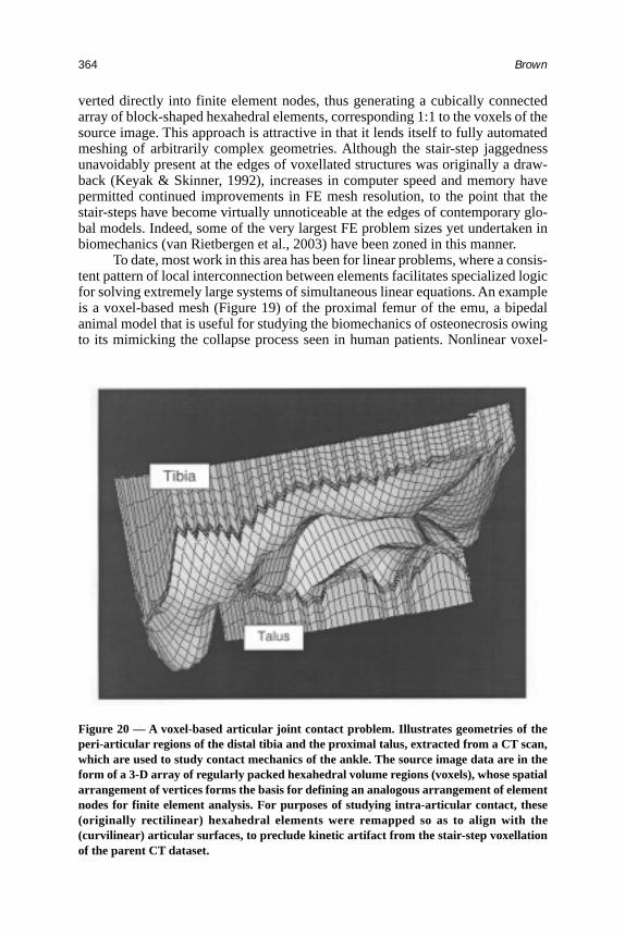
Figure 20 — A voxel-based articular joint contact problem. Illustrates geometries of theperi-articular regions of the distal tibia and the proximal talus, extracted from a CT scan,which are used to study contact mechanics of the ankle. The source image data are in theform of a 3-D array of regularly packed hexahedral volume regions (voxels), whose spatialarrangement of vertices forms the basis for defining an analogous arrangement of elementnodes for finite element analysis. For purposes of studying intra-articular contact, these(originally rectilinear) hexahedral elements were remapped so as to align with the(curvilinear) articular surfaces, to preclude kinetic artifact from the stair-step voxellationof the parent CT dataset.


based formulations have recently begun to appear (Grosland & Brown, 2002) toaddress special situations arising in biomechanics, such as for example patient-specific articular joint contact problems (Figure 20).

Conclusion

Thirty years have now elapsed since the first applications of FEA in biomechanics.There has been ever-accelerating growth in sophistication of the formulationsemployed, and ever-improving realism of the resulting simulations. These improve-ments have been powered by truly prodigious improvements in the capabilities ofcomputing platforms. In the ever-changing world of computer technology, per-haps the one anchor of stability has been that the cost of implementing a givenarithmetic operation has historically dropped by about 50% every 6 months. Theensuing unrelenting treadmill of hardware and software obsolescence is widelyregarded as a much-more-than-acceptable price to pay for the ever-widening op-portunities thus opened. Finite element analysis therefore remains a thriving areaof growth in the field of biomechanics, with no end in sight.

References

Argyris, J.H., & Kelsey, S. (1954). Energy theorems and structural analysis. Aircraft Engi-neering, 26-27 (Oct. 1954–May 1955).

Bathe, K-J. (1996). Finite element procedures. Englewood Cliffs, NJ: Prentice Hall.Brekelmans, W.A.M., Poort, H.W., & Sloof, T.J.J.H. (1972). A new method to analyze the

mechanical behavior of skeletal parts. Acta Orthopaedica Scandinavica, 43, 301-307.

Brown, T.D., Way, M.E., & Ferguson, A.B., Jr. (1981). Mechanical characteristics of bonein femoral capital aseptic necrosis. Clinical Orthopaedics and Related Research,156, 240-247.

Ciarelli, M.J., Goldstein, S.A., Kuhn, J.L., Cody, D.D., & Brown, M.B. (1991). Evaluationof orthogonal mechanical properties and density of human trabecular bone from majormetaphyseal regions with materials testing and computed tomography. Journal ofOrthopaedic Research, 9, 674-682.

Clough, R.W. (1960). The finite element method in plane stress analysis. Proceedings of2nd ASCE Conference on Electronic Computation (pp. 345-378). Pittsburgh, PA.

Cowin, S.C., & Sadegh, A.M. (1991). Non-interacting modes for stress, strain, and energyin ansiotropic hard tissue. Journal of Biomechanics, 24, 859-867.

Grosland, N.M., & Brown, T.D. (2002). A voxel-based formulation for contact finite ele-ment analysis. Computer Methods in Biomechanics and Biomedical Engineering, 5,21-32.

Huiskes, R., & Chao, E.Y.S. (1983). A survey of finite element analysis in orthopaedicbiomechanics: The first decade. Journal of Biomechanics, 16, 385-409.

Huiskes, R., & Hollister, S.J. (1993). From structure to process, from organ to cell: Recentdevelopments of finite element analysis in orthopaedic biomechanics. Journal ofBiomechanical Engineering, 115(4B), 520-527.

Keyak, J.H., & Skinner, H.B. (1992). Three-dimensional finite element modelling of bone:Effects of element size. Journal of Biomedical Engineering, 14, 483-489.

Brown366

Maxian, T.A., Brown, T.D., Pedersen, D.R., & Callaghan, J.J. (1996). Adaptive finite ele-ment modeling of long-term polyethylene wear in total hip arthroplasty. Journal ofOrthopaedic Research, 14, 668-675.

Nadzadi, M.E., Pedersen, D.R., Yack, H.J., Callaghan, J.J., & Brown, T.D. (2003). Kine-matics, kinetics, and finite element analysis of commonplace maneuvers at risk fortotal hip dislocation. Journal of Biomechanics, 36, 577-591.

Ricos, V., Pedersen, D.R., Brown, T.D., Ashman, R.B., Rubin, C.T., & Brand, R.A. (1996).Effects of anisotropy and material axis registration on computed strain distributionsin the turkey ulna. Journal of Biomechanics, 29, 261-267.

Rybicki, E.F., Simonen, F.A., & Weis, E.B. (1972). On the mathematical analysis of stressin the human femur. Journal of Biomechanics, 5, 203-215.

Scifert, C.F., Brown, T.D., Pedersen, D.R., Heiner, A.D., & Callaghan, J.J. (1999). Devel-opment and physical validation of a finite element model of total hip dislocation.Computer Methods in Biomechanics and Biomedical Engineering, 2, 139-147.

Scifert, C.F., Noble, P.C., Brown, T.D., Bartz, R.L., Kadakia, N., Sugano, N., Johnston,R.C., Pedersen, D.R., & Callaghan, J.J. (2001). Experimental and computational simu-lation of total hip arthroplasty dislocation. Orthopaedic Clinics of North America,32, 553-567.

Sokolnikoff, I.S. (1956). Mathematical theory of elasticity (2nd ed.). New York: McGrawHill.

Stewart, K.J., Pedersen, D.R., Callaghan, J.J., & Brown, T.D. (2004). Implementing cap-sule representation in a total hip dislocation finite element model. Iowa OrthopaedicJournal, 24, 1-8.

Synge, J.L. (1957). The hypercircle in mathematical physics. London: Cambridge Press.Van Rietbergen, B., Huiskes, R., Eckstein, F., & Ruegsegger, P. (2003). Trabecular bone

tissue strains in the healthy and osteoporotic human femur. Journal of Bone andMineral Research, 18, 1781-1788.

Acknowledgments

Financial assistance was provided by NIH grants AR46601, AR48939, AR49919,and by DePuy, Inc.

The work depicted in the two case studies was performed in collaboration with Drs.Kelly J. Baker, Douglas R. Pedersen, Richard A. Brand, M. James Rudert, Jiro Sakamoto,Karen (Reed) Troy, Nicole M. Grosland, Christopher F. Scifert, Anneliese D. Heiner, JohnJ. Callaghan, and Mr. Mark E. Nadzadi and Mr. Kristofer J. Stewart. Ms. Julie M. Mock andMr. Thomas E. Baer kindly assisted with manuscript preparation.

Documents

Finite Element Modeling in Musculoskeletal Biomechanics · 2004-10-20 · Finite Element Modeling in Musculoskeletal Biomechanics ... by means of finite element analysis, has proven