Embed Size (px)
Citation preview

HAL Id: tel-01537637https://tel.archives-ouvertes.fr/tel-01537637
Submitted on 12 Jun 2017
HAL is a multi-disciplinary open accessarchive for the deposit and dissemination of sci-entific research documents, whether they are pub-lished or not. The documents may come fromteaching and research institutions in France orabroad, or from public or private research centers.
L’archive ouverte pluridisciplinaire HAL, estdestinée au dépôt et à la diffusion de documentsscientifiques de niveau recherche, publiés ou non,émanant des établissements d’enseignement et derecherche français ou étrangers, des laboratoirespublics ou privés.
Finite element modelling and PGD based modelreduction for piezoelectric and magnetostrictive
materialsZhi Qin
To cite this version:Zhi Qin. Finite element modelling and PGD based model reduction for piezoelectric and magne-tostrictive materials. Electronics. Université Pierre et Marie Curie - Paris VI, 2016. English. �NNT :2016PA066566�. �tel-01537637�

This work is licensed under a Creative Commons Attribution-NonCommercial 4.0 International License
Université Pierre et Marie Curie Ecole Doctorale Science Mécanique Acoustique Electronique et Robotique
Laboratoire d’Electronique et Electromagnétisme (L2E)
Finite Element Modeling and PGD Based Model
Reduction for Piezoelectric & Magnetostrictive Materials
Par Zhi QIN
Thèse de Doctorat en Electronique
Présentée et soutenue publiquement le 02.décembre.2016
Devant un jury composé de :
M. Yves MARECHAL Professeur, Grenoble INP Rapporteur
M. Frédéric BOUILLAULT Professeur, Université Paris Sud Rapporteur
M. Stéphane CLENET Professeur, ENSAM Examinateur
Mme. Hélène ROUSSEL Professeur, UPMC Examinateur
M. Zhuoxiang REN Professeur, UPMC Directeur de Thèse
M. Hakeim TALLEB Maître de Conférences, UPMC Co-Encadrant de Thèse

This page is intentionally left blank.

i
Abstract
The energy harvesting technology that aims to enable wireless sensor networks (WSN) to be maintenance-free, is recognized as a crucial part for the next generation technology mega-trend: the Internet of Things (IoT). Piezoelectric and magnetostrictive materials, which can be used in a wide range of energy harvesting systems, have attracted more and more interests during the past few years. This thesis focuses on multiphysics finite element (FE) modeling of these two materials and performing model reduction for resultant systems, based on the Prop-er Generalized Decomposition (PGD).
Modeling these materials remains challenging although research in this area has been under-going over decades. A multitude of difficulties exist, among which the following three issues are largely recognized. First, mathematically describing properties of these materials is com-plicated, which is particularly true for magnetostrictive materials because their properties depend on factors including temperature, stress and magnetic field. Second, coupling effects between electromagnetic, elastic, and thermal fields need to be considered, which is beyond the capability of most existing simulation tools. Third, as systems becoming highly integrated whole-scale simulations become necessary, which means three dimensional (3D) numerical models should be employed. 3D models, on the other hand, quickly turns intractable if not properly built. The work presented here provides solutions in respond to the above challenges.
A differential forms based multiphysics FE framework is first established. Within this frame-work quantities are discreted using appropriate Whitney elements. After discretization, the system is solved as a single block, thus avoiding iterations between different physics solutions and leading to rapid convergences. Next, the linear piezoelectric, and a free energy based nonlinear magnetostrictive constitutive model called Discrete Energy Averaged Model (DE-AM) are incorporated into the framework. Our implementation describes underlying material behaviors at reasonable numerical costs. Eventually, two novel PGD based algorithms for model reduction are proposed. With our algorithms, problem size of multiphysics models can be significantly reduced while final results of very good accuracy are obtained. Our algo-rithms also provide means to handle coupling and nonlinearity conveniently.
All our methodologies are demonstrated and verified via representative examples

This page is intentionally left blank.
iii
Contents
Abstract ............................................................................................................................................. i
Contents .......................................................................................................................................... iii
List of Tables ................................................................................................................................. vii
List of Figures ............................................................................................................................... viii
Chapter 1. Introduction .................................................................................................................... 1
1.1 Energy harvesting in wireless sensor networks ................................................................... 1
1.2 Piezoelectric and magnetostrictive materials ...................................................................... 3
1.2.1 Piezoelectric materials and piezoelectric effects ................................................... 3
1.2.2 Magnetostrictive materials and magnetostrictive effects ..................................... 4
1.3 Review of existing models .................................................................................................. 7
1.3.1 Existing models for piezoelectric materials ......................................................... 7
1.3.2 Existing models for magnetostrictive materials ................................................... 8
1.4 Research objectives and outline ........................................................................................ 10
Chapter 2. Multiphysics Finite Element Modeling ........................................................................ 13
2.1 Preliminaries on finite element modeling .......................................................................... 13
2.1.1 The finite element method ................................................................................. 13
2.1.2 Whitney elements ............................................................................................... 14
2.2 Equilibrium equations ....................................................................................................... 19
2.2.1 Maxwell’s Equations .......................................................................................... 19
2.2.2 Heat conduction equation ................................................................................... 20
2.2.3 Balance of linear momentum ............................................................................. 21
2.3 Piezoelectric model ........................................................................................................... 23
2.3.1 Linear theory of piezoelectricity ........................................................................ 23
Contents
iv
2.3.2 Finite element formulations ............................................................................... 26
2.3.3 Numerical examples ........................................................................................... 31
2.4 Magnetostrictive model ..................................................................................................... 38
2.4.1 Magnetostrictive constitutive equations ............................................................. 38
2.4.2 The discrete energy averaged model .................................................................. 39
2.4.3 Finite element formulations ............................................................................... 42
2.4.4 Numerical examples ........................................................................................... 47
2.5 Chapter summary .............................................................................................................. 53
Chapter 3. PGD Based Model Reduction of Multiphysics Systems .............................................. 55
3.1 Separated representation based model reduction............................................................... 55
3.1.1 The Proper Orthogonal Decomposition ............................................................. 57
3.1.2 The Proper Generalized Decomposition ............................................................ 59
3.2 A non-incremental algorithm for transient magneto-thermal problems ............................ 63
3.2.1 The coupled nonlinear dynamic problem ........................................................... 64
3.2.2 Conventional time integration approach ............................................................ 66
3.2.3 Non-incremental space-time separation approach ............................................. 67
3.2.4 Numerical application ........................................................................................ 72
3.3 A fast algorithm for parametric electro-mechanical problems .......................................... 75
3.3.1 Separated representation of the parametric problem .......................................... 75
3.3.2 The enrichment process ...................................................................................... 77
3.3.3 Updating strategy ............................................................................................... 79
3.3.4 Numerical application ........................................................................................ 80
3.4 Chapter summary .............................................................................................................. 84
Conclusions and Prospective ......................................................................................................... 87
Appendix A .................................................................................................................................... 89

Contents
v
Appendix B .................................................................................................................................... 94
Bibliography .................................................................................................................................. 97

This page is intentionally left blank.
vii
List of Tables
Table 2.1. Representation of the elasticity tensor for different materials ................................ 22
Table 2.2. Constants for piezoelectric and substrate layers ..................................................... 33
Table 2.3. Constants for the magnetostrictive material............................................................ 49
Table 3.1. Material constants in the inductive heating model.................................................. 73
Table 3.2. Algorithm for parametric electro-mechanical problems ......................................... 79
Table 3.3. Comparison in performance of different implementations ..................................... 80
Table 3.4. Study on parameters of iterations ........................................................................... 83
Table 3.5. Study on parameters of enrichments ....................................................................... 84

viii
List of Figures
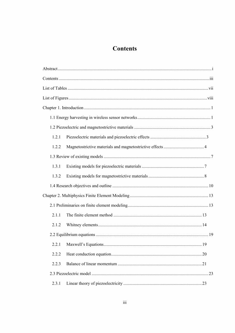
Figure 1.1. A typical scenario of the wireless sensor network [1] ............................................. 1
Figure 1.2. Schematics of (a) piezoelectric, (b) magnetostrictive [2], and (c) magnetoelectric [3] harvester. .............................................................................................................................. 2
Figure 1.3. The (a) direct and (b) inverse piezoelectric effects ................................................. 3
Figure 1.4. Domain structures of piezoelectric ceramics during poling process [6]: (a) before polarization, domains are randomly oriented, (b) domains rearrange along the electric field direction during polarization, and (c) remnant polarization presents after the poling field is removed. .................................................................................................................................... 4
Figure 1.5. Cross section of a Terfenol-D transducer [10] ........................................................ 5
Figure 1.6. Magnetization process in monolythic Terfenol-D [10] ........................................... 6
Figure 1.7. Development of magnetostriction [10] .................................................................... 6
Figure 2.1. Numbering of Whitney elements on a tetrahedron ................................................ 18
Figure 2.2. Electric and mechanical domains of the multiphysics problem ............................ 26
Figure 2.3. The cantilevered bimorph. (a) model configuration, (b) triangulation .................. 32
Figure 2.4. Real and imaginary parts of the first six vibration mode shapes. Displacements are represented by (scaled) deviations from original positions whereas potentials by colored regions (in 𝑉). .......................................................................................................................... 34
Figure 2.5. Output voltage (left) and power (right) of the bimorph versus frequency for different loads .......................................................................................................................... 35
Figure 2.6. A delay-line structured surface acoustic wave transducer. (a) top view and (b) lateral view ............................................................................................................................... 35
Figure 2.7. Displacements in the 𝑧 direction of points A and B .............................................. 37
Figure 2.8. Wave amplitude versus propagation distance (attenuation proportional to slopesof the lines) ............................................................................................................................... 37
Figure 2.9. Simulation results of nonhysteretic magnetization (right) and magnetostriction (left) for <100>𝐹𝑒81.5𝐺𝑎18.5 at various stress (top) and field (bottom) values ...................... 42
Figure 2.10. Domains of the magnetostrictive problem ........................................................... 42
Figure 2.11. Configuration of the TEAM Problem 7 ............................................................... 47

List of Figures
ix
Figure 2.12. Simulation results for the Teamwork Problem 7. (a) source current density in the coil, (b) magnetic flux density around the coil, and (c) induced eddy currents in the conductor ................................................................................................................................................. 48
Figure 2.13. Rsults of the linear magnetostrictive problem (coordinates along the lengthdirection are scaled for representation purpose). (a) edges on which nonzero Dirichlet boundary conditions for 𝐴 are applied; (b) solution of the problem in which arrows depict the magnetic flux distribution whereas the rainbow colored region depicts mechanical deformation; (c) distribution of the magnetic flux density. ..................................................... 50
Figure 2.14. Modeling hierarchy involving FEM on macroscopic, and DEAM on microscopic structure. .................................................................................................................................. 51
Figure 2.15. Convergence study of the piecewise linear strategy. ........................................... 53
Figure 3.1. The non-incremental space-time separated algorithm. .......................................... 72
Figure 3.2. Snapshots of eddy currents during the first (1-9 𝑚𝑠) and ninth period (91-99 𝑚𝑠). ................................................................................................................................................. 73
Figure 3.3. Results from different sets of simulations for (a) the magnetic and (b) thermal problem. ................................................................................................................................... 74
Figure 3.4. Schema of approximating solutions of three-way arrays with low-order tensors. 75
Figure 3.5. Convergence of enrichment process for PGD approach with and without updating. ................................................................................................................................................. 81
Figure 3.6. Components related to spatial coordinates of the first to eighth enrichment. Displacements are depicted by the (scaled) deformation from original positions, while potentials are represented using the colored region. As in Figure 2.4, area for air is not shown in the figure. Values are normalized. ....................................................................................... 82
Figure 3.7. Components related to frequencies of the first to eighth enrichment (Values are normalized). ............................................................................................................................. 82
Figure 3.8. Components related to resistor (𝑅 = 91 𝑘Ω) of all enrichments. .......................... 83

This page is intentionally left blank.
1
Chapter 1. Introduction
In this chapter, introduction to the research background and motivation are given. Specifically, the concepts of WSN and energy harvesting technologies are introduced in section 1. We briefly review properties of piezoelectric and magnetostrictive materials in section 2. A survey of exist-ing models for these materials, especially those used in energy harvesting, is given in section 3, which also explains our motivation of 3D multiphysics FE modeling and models reduction. The chapter concludes with research objectives and outline of the thesis.
1.1 Energy harvesting in wireless sensor networks
Figure 1.1. A typical scenario of the wireless sensor network [1]
With the ever-increasing computing power over the last decade, WSN, recognized as a key ena-bling technique for the IoT, has been applied in applications like environmental monitoring, object tracking and body networks. It is predicted that commercial use of WSN will be perva-sive in the coming years [1].
A typical WSN scenario is depicted in Figure 1.1 where a large number of sensor nodes are deployed for data acquiring. The collected data are processed on the node before sent to a base station, which are finally accessed by end users through the Internet. Such sensor nodes gather and transfer data, thereby consuming considerable energy. While modern sensors are energeti-
Chapter 1. Introduction
2
cally low consuming, power supply can still be an issue. This is because some of them are ex-pected to work for several years, during which period, maintenance of the power units is diffi-cult, or even impossible in many situations. As a result, batteries are no more adequate in this regard. On the contrary, energy harvesting technologies are promising as they require little even zero human intervention.
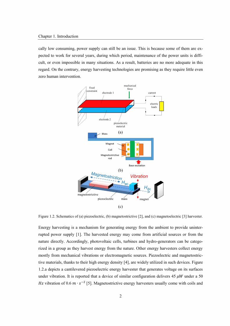
Figure 1.2. Schematics of (a) piezoelectric, (b) magnetostrictive [2], and (c) magnetoelectric [3] harvester.
Energy harvesting is a mechanism for generating energy from the ambient to provide uninter-rupted power supply [1]. The harvested energy may come from artificial sources or from the nature directly. Accordingly, photovoltaic cells, turbines and hydro-generators can be catego-rized in a group as they harvest energy from the nature. Other energy harvesters collect energy mostly from mechanical vibrations or electromagnetic sources. Piezoelectric and magnetostric-tive materials, thanks to their high energy density [4], are widely utilized in such devices. Figure 1.2.a depicts a cantilevered piezoelectric energy harvester that generates voltage on its surfaces under vibration. It is reported that a device of similar configuration delivers 45 𝜇𝑊 under a 50 𝐻𝑧 vibration of 0.6 𝑚 ∙ 𝑠 [5]. Magnetostrictive energy harvesters usually come with coils and

1.2. Piezoelectric and magnetostrictive materials
3
magnets, as shown in Figure 1.2.b. They can also be used to transfer mechanical vibration into electrical energy, while they are less advantageous than piezoelectric harvesters in terms of min-iaturization of volume, due to the existence of coils and magnets. Piezoelectric and magneto-strictive materials can be combined and utilized as magnetoelectric composites (see Figure 1.2.c). In such devices, the magnetostrictive layer generates strain in respond to a varying mag-netic field. Due to inter-layer elastic bonding, the strain passes to the piezoelectric layer that eventually generates electrical charges. It can also harvester energy from mechanical vibration.
1.2 Piezoelectric and magnetostrictive materials
1.2.1 Piezoelectric materials and piezoelectric effects
Piezoelectric materials refer to non-conducting ferroelectric materials that produce electric charges on the surface when mechanical stress is applied, and conversely, produce mechanical strain when electric field is applied, as represented in Figure 1.3 where 𝑃 is the polarization. The stress to charge conversion is called the direct piezoelectric effect, while the other is called the inverse piezoelectric effect.
Figure 1.3. The (a) direct and (b) inverse piezoelectric effects
Piezoelectric materials can be categorized into inorganic, organic and composite types [6]. Pie-zoelectric monocrystalline materials and piezoelectric ceramics fall into the first category. Pie-zoelectric single crystals (e.g. quartz) are commonly seen in e.g. high-selectivity filters and high-temperature ultrasonic transducers because of their high mechanical quality factor and excellent stability. Their applicability is limited due to low piezoelectric coefficients and low machining properties. Piezoelectric ceramics (e.g. lead zirconate titanate, or PZT), on the other hand, possess strong piezoelectricity and can be easily formed into various shapes, although

Chapter 1. Introduction
4
they suffer from low mechanical quality factor and large electric loss. This enables them to be used in high-power transducers and wide-band filters. In the organic piezoelectric group (also referred to as piezoelectric polymers), the polyvinylidene fluoride, or PVDF is probably the most famous. These materials are flexible, low-weight and having small impedance. They are widely used for underwater ultrasonic measuring, pressure sensing, etc. For piezoelectric com-posites, in which piezoelectric ceramics and polymers are bonded together, properties of indi-vidual materials are enhanced. For instance, they can have both strong coupling coefficients and outstanding machining properties, which makes them ideal to be fabricated into large area films or other sophisticated applications [6]. Application of piezoelectric materials in energy harvest-ing systems can be found in [7].
Figure 1.4. Domain structures of piezoelectric ceramics during poling process [6]: (a) before polarization, domains are randomly oriented, (b) domains rearrange along the electric field direction during
polarization, and (c) remnant polarization presents after the poling field is removed.
Piezoelectric effects can be explained from a microscopic point of view. Roughly speaking, they are structurally asymmetric in crystalline, making the electrical domains (see Figure 1.4), which are separated by walls along spontaneous polarization directions, randomly distributed at the original state. Applying increasingly larger electric fields makes these electric domains gradual-ly align with the field, which also results in macroscopic change in shape due to the movements of domains. This procedure is called polarization. Meanwhile, applying mechanical stress caus-es reallocation of electrical walls and as a result, generating macroscopic polarization, or volt-age on the surface. Although piezoelectric coupling is determined by several factors such as temperatures, stresses and fields, the piezoelectric effect can be regarded as linear over a wide range of conditions. We only consider linear piezoelectric behaviors in the thesis.
1.2.2 Magnetostrictive materials and magnetostrictive effects
Magnetostrictive materials refer to those exhibiting magnetostrictive effects that are found in ferromagnetic materials. Magnetostrictive effects consist of two mechanisms: the Joules effect
1.2. Piezoelectric and magnetostrictive materials
5
and the Villari effect [8]. The former implies that rotation of moments to align with an applied field generates strains, while the latter implies that applied stresses cause magnetic moments to rotate thus changing the magnetization. There has been various research on magnetostrictive effects and materials (see e.g. [9]), while we restrict ourselves to giant magnetostrictive materi-als whose magnetostrictive effects are more significant.
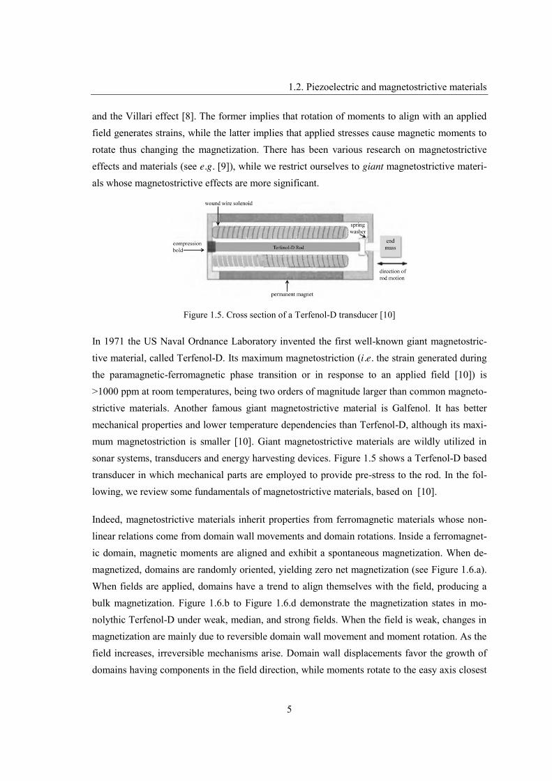
Figure 1.5. Cross section of a Terfenol-D transducer [10]
In 1971 the US Naval Ordnance Laboratory invented the first well-known giant magnetostric-tive material, called Terfenol-D. Its maximum magnetostriction (i.e. the strain generated during the paramagnetic-ferromagnetic phase transition or in response to an applied field [10]) is >1000 ppm at room temperatures, being two orders of magnitude larger than common magneto-strictive materials. Another famous giant magnetostrictive material is Galfenol. It has better mechanical properties and lower temperature dependencies than Terfenol-D, although its maxi-mum magnetostriction is smaller [10]. Giant magnetostrictive materials are wildly utilized in sonar systems, transducers and energy harvesting devices. Figure 1.5 shows a Terfenol-D based transducer in which mechanical parts are employed to provide pre-stress to the rod. In the fol-lowing, we review some fundamentals of magnetostrictive materials, based on [10].
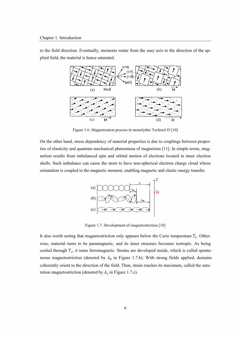
Indeed, magnetostrictive materials inherit properties from ferromagnetic materials whose non-linear relations come from domain wall movements and domain rotations. Inside a ferromagnet-ic domain, magnetic moments are aligned and exhibit a spontaneous magnetization. When de-magnetized, domains are randomly oriented, yielding zero net magnetization (see Figure 1.6.a). When fields are applied, domains have a trend to align themselves with the field, producing a bulk magnetization. Figure 1.6.b to Figure 1.6.d demonstrate the magnetization states in mo-nolythic Terfenol-D under weak, median, and strong fields. When the field is weak, changes in magnetization are mainly due to reversible domain wall movement and moment rotation. As the field increases, irreversible mechanisms arise. Domain wall displacements favor the growth of domains having components in the field direction, while moments rotate to the easy axis closest
Chapter 1. Introduction
6
to the field direction. Eventually, moments rotate from the easy axis to the direction of the ap-plied field, the material is hence saturated.
Figure 1.6. Magnetization process in monolythic Terfenol-D [10]
On the other hand, stress dependency of material properties is due to couplings between proper-ties of elasticity and quantum mechanical phenomena of magnetism [11]. In simple terms, mag-netism results from imbalanced spin and orbital motion of electrons located in inner electron shells. Such imbalance can cause the atom to have non-spherical electron charge cloud whose orientation is coupled to the magnetic moment, enabling magnetic and elastic energy transfer.
Figure 1.7. Development of magnetostriction [10]
It also worth noting that magnetostriction only appears below the Curie temperature 𝑇 . Other-
wise, material turns to be paramagnetic, and its inner structure becomes isotropic. As being cooled through 𝑇 , it turns ferromagnetic. Strains are developed inside, which is called sponta-neous magnetostriction (denoted by 𝜆 in Figure 1.7.b). With strong fields applied, domains
coherently orient to the direction of the field. Then, strain reaches its maximum, called the satu-ration magnetostriction (denoted by 𝜆 in Figure 1.7.c).

1.3. Review of existing models
7
1.3 Review of existing models
1.3.1 Existing models for piezoelectric materials
1.3.1.1 Piezoelectric constitutive models
Although hysteresis and nonlinearity are intrinsic for piezoelectric constitutive relations, a cou-ple of mechanisms (e.g. keeping the material in low or moderate operating regimes to linearize the response) can be employed to reduce hysteretic and nonlinear effects. More importantly, polarization and fields generated with the direct piezoelectric effect, which is of main concern in our context, exhibit an almost linear dependence on the stress for low input levels [10]. All in all, the linear piezoelectric constitutive model, which relates dielectric and elastic behaviors of piezoelectric materials, provides sufficient accuracy in most cases. Therefore, we only use the linear model. More details of this model will be presented in the next chapter when we develop piezoelectric FE models.
1.3.1.2 Piezoelectric system models
Generally, piezoelectric system models can be divided into lumped-parameter type and FE type. For the former, lumped parameters for the electric domains can be easily obtained due to the inherent capacitance of piezoelectric materials and resistances from the external load. For the mechanical domain, a single mechanical degree of freedom is usually employed for the predic-tion of system dynamics. As long as the mechanical domain lumped-parameters are available, mechanical and electric equilibrium equations can be coupled via piezoelectric constitutive equations, leading to transformer relations (see e.g. [12] for details). While such methods pro-
vide initial insights into the coupled system through solving computationally cheap equations, the solutions lack some important aspects, such as the dynamic mode shapes, accurate strain distribu-tion, and effects of the latter two on the electrical side [13].
FE models (see e.g. [14]), on the other hand, are more advantageous as they are more flexible to model complicated configurations and capable to obtain full field numerical solutions. With this method, weak forms are generated based on equilibrium and constitutive equations. The result-ing infinite dimensional problem is then projected onto finite dimensions. As such, the problem amounts to solving a discrete system. At the same time, FE methods are also computationally more intensive, especially for large 3D models. Therefore, developing model order reduction techniques that preserve versatilities of the FE method while alleviate the computational burden, seems like a prospective approach.
Chapter 1. Introduction
8
1.3.2 Existing models for magnetostrictive materials
1.3.2.1 Magnetostrictive constitutive models
As summarized in [15], early magnetostrictive constitutive models consist in adapting ferro-magnetic models to incorporate magnetoelastic couplings. Examples are the modified Preisach model and Jiles-Atherton model. In the latter, for instance, the effect of stress on magnetization is incorporated through adding a stress-equivalent field term into the modified Langevin equa-tion. These models can be used to simulate e.g. variation of magnetization with stress. However, they are, to some extent, purely mathematical tools that do not address the underlying physics with sufficient accuracy. There are also a class of free-energy models for uniaxial cases [15]. In these models, the Gibbs energy for a given applied field is expressed in function of magnetiza-tion, and additional terms that were created to incorporate stress effects. This class of models is reported to be more suited to explain the physics of hysteresis rather than realistic simulations.
In [16] a new energy-based model called the modified Armstrong model is introduced. The idea is to construct magnetocrystalline, magnetoelastic and magnetic field energy terms. Sum of the latter terms corresponding to magnetization of different orientations is evaluated. The probabil-ity of a certain magnetization orientation is determined with respect to (w.r.t.) the total energy of that orientation, the lower its total energy is the larger that probability will be. Macroscopic properties of the material can be obtained as averages of all possible orientations. Therefore, accurate evaluation of macroscopic properties requires considering a large number of such ori-entations. The modified Armstrong model is based on 98 such orientations. A further improve-ment is proposed in [17] where the number of orientation is reduced to six. This model is named the Discrete Energy-Averaged Model, or DEAM. It has been validated for Galfenol [18] and Terfenol-D [19]. Compared with other magnetostrictive constitutive models, DEAM is advanta-geous due to its accuracy and ease to be elaborated into a FE framework. Although there are other magnetostrictive constitutive models, they are generally one dimensional or, more or less, do not properly address the underlying physics.
1.3.2.2 Magnetostrictive system models
As introduced above, magnetostrictive materials are normally inhomogeneous. Consequently, modeling magnetostrictive devices involves a hierarchy of structures on different levels – con-stitutive modeling on the microscopic level and system modeling on the macroscopic level. Here constitutive modeling refers to the calculation of material constants, whereas system mod-eling refers to the calculation of state variables (e.g. magnetic fields and stresses). As with the
1.3. Review of existing models
9
piezoelectric case, popular magnetostrictive system modeling approaches can be categorized into the lumped-parameter type and the FE type. However, with the former type it is difficult, or impossible, to account for material inhomogeneity. Therefore, only FE models are reviewed.
Among the reported magnetostrictive models, a considerable amount of them are implemented using commercial packages e.g. COMSOL Multiphysics. Take the latter for example; single field interfaces are predefined while couplings need to be established via e.g. initial stress and remanant flux density features. Values of initial stresses and remanant flux densities are speci-fied as functions of respectively, magnetic field and mechanical strain [20]. With this approach, incorporating material constitutive relations or any other un-predefined features can be cumber-some, if ever possible. Other ones, which do not rely on commercial packages, consist in en-forcing the coupling weakly. For example, in [21] magnetic and elastic problems are resolved individually, while couplings are enforced through magnetic or mechanical excitations. The shortcoming with this approach is evident: data needs to be transferred between physics; itera-tions are also needed to enforce equilibrium, which deteriorates the simulation speed. In [22] a strongly coupled magnetostrictive model is presented. In this model, magnetic and elastic prob-lems are solved simultaneously, using the same mesh, which eventually forms a block of dis-crete equations. Within the block, diagonal parts correspond to individual physics, whereas off-diagonal parts correspond to couplings. Unknowns are mechanical displacements and vector magnetic potentials 𝐴. However, in [22] nodal elements are used to discretize 𝐴. This can be improved through discretizing 𝐴 using Whitney elements, or vector basis functions [23]. Anoth-er issue with the model in [22] is that the electrical potential 𝜙 is not considered, while it is proved that the 𝐴- 𝜙 formulation is more appropriate regarding stability and convergence rate, especially for magneto-dynamic problems [24].
Magnetostrictive FE models are also commonly found in literatures of two-phase magnetoelec-tric laminated composites. This is because in the latter, magnetostrictive and piezoelectric mate-rials are combined via strain, due to which magnetoelectric modeling is, in fact, combination of individual magnetostrictive and piezoelectric modeling. For example, in [25] a nonlinear but two dimensional (2D) FE magnetostrictive model is presented. In this model magnetostriction is assumed to be a parabolic function of the magnetization, while a Langevin-type equation is employed to consider relations between magnetization and magnetic field. In our own research group, 2D nonlinear magnetostrictive models are also developed, in the context of magnetoelec-tric modeling, where the effect of load impedances in magnetoelectric devices can be accounted for [26]. As a first attempt, the Brauer model describing the initial magnetization curve is used.
Chapter 1. Introduction
10
This model gives good predictions for devices of various volume ratios, epoxy bonding materi-als, and bias fields. Recently, this approach is extended to model Rosen-type devices [27]. While these models are effective in certain cases, there is no doubt that a fully coupled 3D mag-netostrictive model which better incorporates material nonlinearities and multiphysics couplings is indispensable.
1.4 Research objectives and outline
Our ultimate objective of the thesis is to build a 3D FE framework, in which piezoelectric and magnetostrictive materials involved multiphysics problems can be modeled and simulated. To this end, several challenges, as mentioned previously, shall be addressed.
x The first one lies in constitutive modeling. For piezoelectric materials, constitutive equa-tions based on linear piezoelectricity can be utilized. Elaborating the latter into FE systems is also well explained in numerous piezoelectric modeling literatures. For magnetostrictive materials, the state-of-the-art constitutive models are energy-based. These models are favor-able because they better describe underlying physics of the material, and are applicable for a larger range of cases. However, elaborating them into FE systems can be also very compu-tationally expensive, due to the involvement of a hierarchy of multi-level modeling. More precisely, the magnetostrictive constitutive model is fed with state variables (usually includ-ing stress and magnetic field strength) at a specific location, and gives as outputs material constants for that location. State variables can be solved with FE models on the macroscopic level, while solving the constitutive model takes place on microscopic level. Therefore, for a given profile of state variables the microscopic problem needs to be solved a lot of times (in fact, as many as the number of microscopic volumes consisted in the system), not to mention possible involvements of nonlinearity (resulted from the recursive dependency of state variables in the FE system). As such, the objective is to implement constitutive models in an efficient way, so that solutions on the microscopic level do not deteriorate the simula-tion speed while integration of constitutive models and FE models is convenient.
x Another challenge comes from involvements of multiphysics fields including electromag-netic, elastic, thermal, and electric circuits. Without doubt, for problems with single fields dedicated FE methodologies are vastly available. By contrast, the availability becomes questionable when multiple physics and coupling in between need to be considered. We note that in a differential forms based FE framework, the problem can be easily resolved. In

1.4. Research objectives and outline
11
such a framework, quantities of different type are discretized using appropriate types of el-ements, called Whitney elements. Properties on the continuous level can be preserved after discretization. In addition, problems of different fields can be modeled in a unified fashion; boundary conditions that are normally tedious to handle with conventional FEs can also be handled straightforwardly. Hence, we define our second objective to be establishing a dif-ferential forms based FE framework, in order to elaborate piezoelectric and magnetostric-tive problems into the 3D numerical system. Meanwhile, thermal fields and electric circuit related models shall be incorporated in this framework, so that we can investigate, for ex-ample, effects of thermal losses and load impedances in a piezoelectric/magnetostrictive materials based system.
x While 3D FE models are superiors compared with their counterparts, in terms of providing full-field solutions, dealing with complicated geometries and boundary conditions, etc., they can also be problematic because of their large model size. For this reason, it is vital to de-velop corresponding model reduction techniques, with which advantages of FE models can be preserved while at affordable computing costs. We noticed that PGD is adequate to this end. Indeed, high computational costs of 3D multiphysics FE simulation frequently come in two flavors. One consists in solving the large system repeatedly in a similar setting, such as in the case of transient analysis where the number of time steps is huge. The other consists in solving the large system for a large number of times in different settings, for example, in the case of parametric analysis where the number of parameters is large. PGD tackles these problems through decomposition, with which the original large-size problem can be con-verted to a series of smaller-size sub-problems, thereby significantly reducing the problem complexity. Our third objective with PGD is to develop efficient algorithms so that transient and parametric simulations using our multiphysics FE models can be performed as efficient-ly as possible.
With these objectives in mind, we have accomplished a couple of contributions that are present-ed in the remainder of the thesis.
In Chapter 2, we describe our implementation of the multiphysics framework and constitutive models. Some preliminaries of FE modeling including the principle procedures of an FE analy-sis, and Whitney elements, are first provided. Introduction of equilibrium equations of electro-magnetic, elastic and thermal fields, which are incorporated in our framework, comes aftermath. In § 2.3, we present our piezoelectric model. The model is based on linear piezoelectricity, with electrodes and electric loads considered. Unknowns of the model are mechanical displacements

Chapter 1. Introduction
12
and elastic potentials, which are interpolated using the nodal Whitney elements. Simulations of a piezoelectric bimorph and a surface acoustic wave (SAW) device are presented. In § 2.4, we introduce our magnetostrictive model. More precisely, we review some fundamentals of DEAM and describe our implementation of it. After that, FE models of magnetostrictive materials, as well as elaboration of DEAM into the latter are discussed. In our model, the 𝐴 − 𝜙 formulation for magnetodynamics is used. Various elements including the nodal, edge, and facet Whitney elements are employed for discretization of involved quantities. Simulations of both linear and nonlinear magnetostrictive problems are presented. FE formulations of these models for linear tetrahedron elements are provided.
In Chapter 3, model reduction via separated representations is first reviewed. Basics of PGD and the method closely related to it – Proper Orthogonal Decomposition (POD) are briefly re-visited. Our two PGD-based novel algorithms are then presented. The first one is dedicated to nonlinear magneto-thermal transient analysis, in which time constants of different fields are orders of magnitude different, and thus resulting in a large number of time steps. Our proposi-tion is to decompose quantities into space and time associated components, with which the orig-inal problem of solving a large space system at sequential time steps is converted to solving space system and time system alternatively, thereby reducing the problem complexity. The sec-ond algorithm is dedicated to parametric electro-mechanical analysis. For such problems, the number of parameters is large, due to which the large-size FE system have to be solved for as many times, being extremely time-consuming. Our solution is to decompose ensemble of the problem into components associated with different parameters, after which we solve a series of smaller-size problems to obtain approximate solutions. At the end of the chapter, we also dis-cuss extension of the above algorithms to other applications.
In the last chapter, conclusions and prospective of the thesis are provided.
13
Chapter 2. Multiphysics Finite Element Modeling
In this chapter, we present our multiphysics FE models for piezoelectric and magnetostrictive materials. Preliminaries on FEM are provided in section 1, with emphasis on Whitney ele-ments. Next, equilibrium equations used for electromagnetic, elastic and thermal fields are revisited in section 2. The piezoelectric model is presented in section 3. Applications of the model on investigation of a bimorph and a SAW device are also described. Section 4 deals with the magnetostrictive model. Introduction to DEAM (as well as the implementation for it) and FE formulations are presented separately. Elaborating DEAM into the FE system is ex-plained through a nonlinear magnetostrictive problem. Applications of the magnetostrictive model for source current involved problems and harmonic analysis are also presented.
2.1 Preliminaries on finite element modeling
2.1.1 The finite element method
FEM is a numerical technique for finding approximate solutions to boundary value problems (BVPs) that are defined in terms of partial differential Equations (PDEs). FEM was first de-veloped in the 1950s and is nowadays utilized in various domains, thanks to their flexibility in modeling complicated geometry and capability in obtaining full field numerical solutions. Generally, a FE analysis can be divided into the following steps:
x Construct PDEs governing the problem of interest, based on physical laws; identifyboundary and initial conditions of the problem.
x Build weak forms, using either the variational method or weighted residue methods,through which an error function associated with the approximated solutions is minimized.
x Triangulate the domain into simplex that are called finite elements; over each element,interpolate quantities with degrees of freedoms and FE basis functions.
x Sum the interpolants over the triangulation, which leads to a system of matrix energetical-ly equivalent to the weak form; resolve the discrete system.
x Post-process, analyze the results, etc.
In the remainder of the thesis, we apply FEM to specific problems, for which the convention
Chapter 2. Multiphysics Finite Element Modeling
14
of notation are as follows. We use (in the majority of the cases) lower case letters e.g. 𝑎 to denote scalars, bold lower case letters e.g. 𝒂 and plain capital letters e.g. 𝐴 to denote vectors, bold capital letters e.g. 𝑨 to denote matrices, and calligraphic letters e.g. 𝔄 to denote tensors of order higher than two (that shall appear in Chapter 3).
2.1.2 Whitney elements
For certain multivariable calculus problems, particularly electromagnetics, it is more direct to solve with differential forms than vector calculus. Because with the former, field properties such as curl-free or divergence-free, and appropriate continuity across material interfaces are preserved [28]. More importantly, when the system is discretized with differential forms based elements, which are called Whitney elements [29], the favorable characteristics can be inherited from the continuous to discrete level. In this part, differential forms and Whitney elements, particularly linear tetrahedral elements, are briefly introduced. More comprehensive treatment on these topics can be found in, e.g. [30], [31] and [32]. Here, we follow [28].
2.1.2.1 Differential forms
In differential forms calculus, four types of entries called 𝑝-forms are utilized in 3D applica-tions. Among them the 0-form and 3-form are scalar quantities whilst the 1-form and 2-form are vector quantities. Roughly speaking, a 𝑝-form takes a 𝑝-dimensional vector and gives a number. Each type of 𝑝-form belongs to a specific functional space, called Hilbert space. Meanwhile, various operators, corresponding to those in vector calculus, are defined on 𝑝-forms. For instance, the exteriors derivative, a metric free operator, corresponds to the gradi-ent, curl and divergence in vector calculus. The wedge operator ∧, also called exterior prod-uct, corresponds to the dot and cross products. Other frequently used operators including the Hodge star operator ⋆ , the pullback and push-forward operators are mainly used for coordi-nate transformations [28]. Properties of 𝑝-forms are summarized as follow.
𝜔 ∶= 𝛽(𝑦)d𝑥 ∧ d𝑥 ∧ d𝑥 (2.1)
The 3-form is integrated over a volume and constant in the volume. It is best suited to repre-sent quantities like scalar densities. A 3-form is shown in Equation (2.1) where (𝑥 , 𝑥 , 𝑥 ) is the basis of a manifold in ℝ , (d𝑥 , d𝑥 , d𝑥 ) the basis of the cotangent space of the man-ifold, 𝑦 a point in ℝ , and 𝛽 the value at 𝑦.
2.1. Preliminaries on finite element modeling
15
ℒ (Ω) ∶= 𝑢; 𝑢 𝑑Ω < ∞
‖𝑢‖ℒ ∶= (‖𝑢‖ ) /
(2.2)
The Hilbert space where 𝜔 lives in, is denoted by ℒ whose definition and associated normare shown in Equation (2.2).
A 0-form, as in Equation (2.3), is defined on a point, giving a scalar of the function at that point. It is utilized to represent potential variables as it is continuous along all orientations.
𝜔 ∶= 𝛽(𝑦) (2.3)
Concurrently a continuous scalar function represented by 𝜔 , belongs to the functional spaceℋ(grad) whose definition and norm are shown in Equation (2.4).
ℋ(grad, Ω) ∶= 𝑢: 𝑢 ∈ ℒ (Ω); grad(𝑢) ∈ ℒ (Ω)
‖𝑢‖ℋ( , ) ∶= (‖𝑢‖ + ‖grad(𝑢)‖ ) /(2.4)
The 1-form, as shown in Equation (2.5), is integrated over a line. It has tangential continuity which makes it suited for the representation of field quantities such as electric field.
𝜔 ∶= 𝛽 (𝑦)d𝑥 + 𝛽 (𝑦)d𝑥 + 𝛽 (𝑦)d𝑥 (2.5)
Functions expressed as 1-forms are defined in the functional space ℋ(curl) whose definition and associated norm are presented in Equation (2.6).
ℋ(curl, Ω) ∶= 𝑈: 𝑈 ∈ ℒ (Ω) ; curl(𝑈) ∈ ℒ (Ω)
‖𝑈‖ℋ( , ) ∶= (‖𝑈‖ + ‖curl(𝑈)‖ ) /(2.6)
Chapter 2. Multiphysics Finite Element Modeling
16
The 2-form, integrated over surfaces, has the form of Equation (2.7). It is continuous in the normal direction, making it suitable for representing flux quantities.
𝜔 ∶= 𝛽 (𝑦)d𝑥 ∧ d𝑥 + 𝛽 (𝑦)d𝑥 ∧ d𝑥 + 𝛽 (𝑦)d𝑥 ∧ d𝑥 (2.7)
Objects expressed as a 2-form is defined in the functional space ℋ(div), as depicted in (2.8).
ℋ(div, Ω) ∶= 𝑈: 𝑈 ∈ ℒ (Ω) ; div(𝑈) ∈ ℒ (Ω)
‖𝑈‖ℋ( , ) ∶= (‖𝑈‖ + ‖div(𝑈)‖ ) /(2.8)
Between differential forms the exterior derivative is defined, which linearly maps a 𝑝-form to a (𝑝 + 1)-form, as expressed in Equation (2.9).
d: Λ → Λ ; 𝜔 ↦ d𝜔 (𝑝 = 0,1,2) (2.9)
An exact sequence of 𝑝-forms can be generated with the exterior derivative operator, as de-picted in Equation (2.10) where corresponding derivative operators in vector calculus are shown in blue. The sequence suggests that the exterior derivative of a 𝑝-form belongs to a subspace of the space of the (𝑝 + 1)-form.
𝜔d
⟶ (grad)
𝜔d
⟶ (curl)
𝜔d
⟶ (div)
𝜔 (2.10)
Moreover, the generalized Stokes law can be expressed with the exterior derivative operator
d𝜔 = 𝜔 (2.11)
The equation implies that integrating the exterior derivative of an 𝑝-form over the whole man-ifold Ω euqals to the integral of that 𝑝-form over the oriented boundary of the manifold.

2.1. Preliminaries on finite element modeling
17
Namely, the boundary operator and exterior derivative are dual to each other. On the other hand, successively applying the exterior derivative results in the trivial form i.e. d(d𝜔 ) = 0. Physically, this correlates to, for example, the curl-free property of the electric field and the divergence-free property of the magnetic flux density
2.1.2.2 Whitney elements
The edge elements were initialized by Nédélec [33] while the link between differential forms and FEs was advanced by Bossavit who also created the term Whitney elements [29]. An ex-hausted history review is outside the scope here, but it can be found in e.g. [30]. Here we show the involvement of Whitney elements in discretization via an abstract problem.
Consider a given Hilbert space 𝑉, a bilinear continuous form 𝑎(∙ , ∙) defined on 𝑉 × 𝑉, and a continuous linear form 𝑙(∙) defined on 𝑉. The abstract problem can be defined in the weak form: find 𝑢 ∈ 𝑉, such that 𝑎(𝑢, 𝑣) = 𝑙(𝑣), for all 𝑣 ∈ 𝑉. 𝑉 is the test space of 𝑝-forms with appropriate boundary conditions. Using the Galerkin method, the problem is projected onto a finite dimensional space 𝑉 ⊆ 𝑉, associated with a triangulation of the domain with ℎ charac-terizing the triangulation. The finite dimensional weak form reads: find 𝑢 ∈ 𝑉 , such that 𝑎(𝑢 , 𝑣 ) = 𝑙(𝑣 ), for all 𝑣 ∈ 𝑉 . Denoting the error between the exact solution 𝑢 and the approximation 𝑢 as 𝜖 , the Galerkin orthogonality can be deduced, as in (2.12).
𝑎(𝜖 , 𝑣) ∶= 𝑎(𝑢 , 𝑣 ) − 𝑙(𝑣 ) = 0 (2.12)
The equation implies that the residual, which is obtained by inserting 𝑢 into the original equation and taking the difference between both sides, is orthogonal to the test functional space. In general, bases for 𝑉 and 𝑉 are identical polynomial functions. These functions have compact supports, meaning that each basis function is only nonzero over a specific sub-domain – an eleent 𝒦. The solution 𝑢 over element 𝒦 is interpolated with 𝑁 bases functions on the element and degrees of freedom (DoFs) 𝛼 , as presented in Equation (2.13). Briefly, a FE is the combination of the polynomial space 𝒫, the compact support 𝒦and DoFs.
𝐼𝒦(𝑢) ∶= 𝛼 (𝑢)𝑣 (2.13)
Over the triangulation 𝒯 containing all the elements 𝒦 , the solution 𝑢 is interpolated as the
Chapter 2. Multiphysics Finite Element Modeling
18
sum of local interpolants over each 𝒦 , see Equation (2.14).
𝐼𝒯(𝑢)|𝒦 ∶= 𝐼𝒦 (𝑢), ∀ 𝒦 ∈ 𝒯 (2.14)
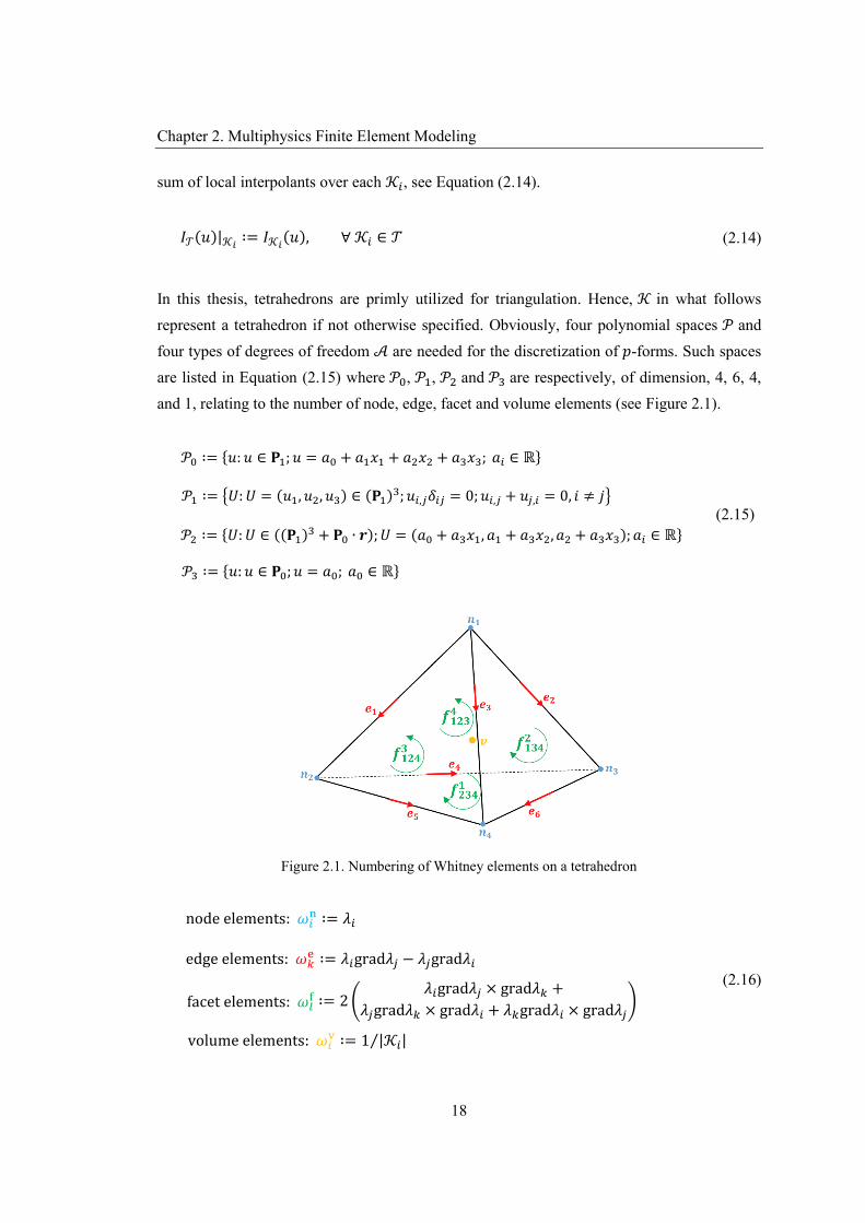
In this thesis, tetrahedrons are primly utilized for triangulation. Hence, 𝒦 in what follows represent a tetrahedron if not otherwise specified. Obviously, four polynomial spaces 𝒫 and four types of degrees of freedom 𝒜 are needed for the discretization of 𝑝-forms. Such spaces are listed in Equation (2.15) where 𝒫 , 𝒫 , 𝒫 and 𝒫 are respectively, of dimension, 4, 6, 4,and 1, relating to the number of node, edge, facet and volume elements (see Figure 2.1).
𝒫 ∶= {𝑢: 𝑢 ∈ 𝐏 ; 𝑢 = 𝑎 + 𝑎 𝑥 + 𝑎 𝑥 + 𝑎 𝑥 ; 𝑎 ∈ ℝ}
𝒫 ∶= 𝑈: 𝑈 = (𝑢 , 𝑢 , 𝑢 ) ∈ (𝐏 ) ; 𝑢 , 𝛿 = 0; 𝑢 , + 𝑢 , = 0, 𝑖 ≠ 𝑗
𝒫 ∶= {𝑈: 𝑈 ∈ ((𝐏 ) + 𝐏 ∙ 𝒓); 𝑈 = (𝑎 + 𝑎 𝑥 , 𝑎 + 𝑎 𝑥 , 𝑎 + 𝑎 𝑥 ); 𝑎 ∈ ℝ}
𝒫 ∶= {𝑢: 𝑢 ∈ 𝐏 ; 𝑢 = 𝑎 ; 𝑎 ∈ ℝ}
(2.15)
Figure 2.1. Numbering of Whitney elements on a tetrahedron
node elements: 𝜔 ∶= 𝜆
edge elements: 𝜔 ∶= 𝜆 grad𝜆 − 𝜆 grad𝜆
facet elements: 𝜔 ∶= 2𝜆 grad𝜆 × grad𝜆 +
𝜆 grad𝜆 × grad𝜆 + 𝜆 grad𝜆 × grad𝜆
volume elements: 𝜔 ∶= 1 |𝒦 |⁄
(2.16)

2.2. Equilibrium equations
19
Basis functions of the four types of elements are summarized in Equation (2.16) where 𝜆 indicates the barycentric coordinate associated with the i-th vertex 𝑛 . The value of 𝜆 ranges between 0 and 1, reaching its maximum 1 at 𝑛 and linearly decreasing to 0 on the facet op-posing to 𝑛 . |𝒦 | in the volume element basis function represents the volume of 𝒦 . Formula-tions utilized to calculate barycentric coordinates are listed in § A.1.
Meanwhile, DoFs represent discrete 𝑝-form coefficients. For node elements, they are values of the quantity on the vertices; For edge elements, they are circulations of the field over edges (∫ 𝑈 ∙ 𝒕), where 𝒕 is denotes the unit tangential vector. For facet element, they are flux through facets (∫ 𝑈 ∙ 𝒏), where 𝒏 is a unit outward normal to the boundary of the facet. For volume elements, they are volume integral of the distribution.
It is noted that when interpolants are substituted into the bilinear form in Equation (2.12), the unified single operator – exterior derivative in Equation (2.10) leads to three discrete opera-tors: 𝑮, C and D, called the incident matrices, corresponding to respectively, the gradient, curl and divergence operator in vector calculus. Entries in these discrete operators are 1, 0 or -1, decided by the orientations and incident relations of the involved geometric entries [34].
2.2 Equilibrium equations
Next, we briefly revisit equilibrium equations for multiphysics fields. They are the Maxwell’s Equations for electromagnetic fields, the heat conduction equation for thermal fields, and balance of linear momentum for elastic fields. While differential forms are employed in the previous section, equations here are presented in vector calculus because we use nodal Whit-ney elements, (also called Lagrange elements), for both elastic and thermal quantities in the implementation (other 𝑝-forms based elements are used for electromagnetic quantities), for which vector calculus representations seem to be more common. That being said, differential forms are employed for introduction of Whitney elements, rather than continuous field equa-tions. Nevertheless, thorough differential forms based treatments on the involved problems can be found in literatures. See e.g. [34] on magnetics, [35], [36] on elastics and [37] on thermal problems.
2.2.1 Maxwell’s Equations
Maxwell’s Equations are shown in Equation (2.17). The first is the Maxwell-Ampère’s law;
Chapter 2. Multiphysics Finite Element Modeling
20
second the Faraday’s law; third and fourth respectively, Gauss’ magnetic and electric law. Quantities in the equations can be grouped into three categories – field intensities including electric field 𝐸(𝑉 ∙ 𝑚 ) and magnetic field 𝐻(𝐴 ∙ 𝑚 ), flux densities including electric displacement 𝐷(𝐶 ∙ 𝑚 ), magnetic induction 𝐵(𝑇), and current density 𝐽(𝐴 ∙ 𝑚 ), and vol-ume density - the electric charge density 𝜌 (𝐶 ∙ 𝑚 ). On the discrete side, they are repre-
sented with respectively, edge, facet and volume elements. In practice potentials are em-ployed to express field variables. We use electric potential 𝜑(𝑉) and magnetic vector poten-tial 𝐴(𝑉 ∙ 𝑠 ∙ 𝑚 ). They are represented by node and edge elements, respectively.
curl𝐻 = 𝐽 + 𝜕𝐷 𝜕𝑡⁄
curl𝐸 = − 𝜕𝐵 𝜕𝑡⁄
div𝐵 = 0
div𝐷 = 𝜌
(2.17)
𝐷 = 𝜀 𝐸 + 𝑃
𝐵 = 𝜇 (𝐻 + 𝑀)
𝐽 = 𝜎 𝐸
(2.18)
Field and flux quantities are related by constitutive equations. See Equation (2.18) in which 𝜀 and 𝜇 are the permittivity and permeability of free space, equal to, 8.854∙10-12 (𝐹 ∙ 𝑚) and 4𝜋 ∙10-7 (𝐻 ∙ 𝑚 ), respectively. 𝜎 (𝑆 ∙ 𝑚 ) denotes the electric conductivity.
2.2.2 Heat conduction equation
Heat conduction is governed by
𝜌𝑐 𝜕𝜃⁄𝜕𝑡 + div𝜙 − 𝑠 = 0 (2.19)
in which 𝜌(𝑘𝑔 ∙ 𝑚 ) represents the mass density per unit volume, 𝑐 (𝐽 ∙ 𝐾 ) specific heat capacity at constant pressure, 𝜃(𝐾) temperature, 𝜙(𝑊 ∙ 𝑚 ) heat flux, and 𝑠(𝑊 ∙ 𝑚 ) the rate of heat generation per unit volume. According to the Fourier’s theorem, 𝜙 can be ex-pressed using temperature gradients, as expressed in (2.20) where the minus sign implies flux

2.2. Equilibrium equations
21
flows from higher to lower temperatures.
𝜙 = −𝜅 ∙ grad𝜃 (2.20)
Meanwhile, 𝜅(𝑊 ∙ 𝑚 ∙ 𝐾 ) in the equation represents the thermal conductivity. Substitut-ing the Fourier’s theorem into Equation (2.19) yields Equation (2.21) that, in conjunction with proper initial and boundary conditions, is employed to describe thermal fields.
𝜌𝑐 𝜕𝜃 𝜕𝑡⁄ − div(𝜅 ∙ grad𝜃) − 𝑠 = 0 (2.21)
2.2.3 Balance of linear momentum
The balance of momentum describes movements and deformations of solid matter in spatial coordinates. In general, the basis of the spatial coordinates is denoted by minuscule 𝒙(𝑥, 𝑦, 𝑧). A reference coordinate is also needed in order to describe material properties before solution. The basis of the reference coordinate system is denoted by capitals 𝑿(𝑋, 𝑌, 𝑍).
𝒙(𝑿, 𝑡) = 𝑿 + 𝒖(𝑿, 𝑡) (2.22)
The reference coordinates are constant over solution whereas the spatial coordinates changes. The relation between these two coordinate systems is shown in Equation (2.22) where 𝒖(𝑢, 𝑣, 𝑤) denotes the displacement vector. In this thesis geometric linearity is assumed, which means no distinction between them is made. In other words, equations are formulated w.r.t. the undeformed state. This assumption is viable, as long as deformations are small enough, so that errors introduced by ignoring the deformation are negligible. Accordingly, the Engineering strain, Cauchy stress and linear elastic material models [38] are employed, as addressed below. Otherwise, geometric nonlinearity needs to be considered, which means the reference configuration is updated with deformation after each solution. The Green-Lagrange strain and the Second Piola-Kirchoff stress [38] shall be utilized in the latter case.
To relate displacements with forces, we first introduce the engineering strain tensor 𝜺, as shown in (2.24). Normal strain entries are defined as 𝜀 = 𝜕𝑢 𝜕𝑥⁄ , while shear strain en-tries, which are denoted by 𝜀 satisfying 𝜀 = 𝜀 for 𝑖 ≠ 𝑗. 𝑢 and 𝑥 are components of 𝑢and 𝑥 in Equation (2.22), with 𝑖, 𝑗 = 1,2,3. The symmetric-gradient operator (which is denot-

Chapter 2. Multiphysics Finite Element Modeling
22
ed by grad) is applied to the displacement, to obtain the strain tensor (see the expression incompact form in (2.23) where the superscript ‘𝑡’ implies transpose).
grad 𝒖 ∶= 1 2⁄ (grad 𝒖 + (grad 𝒖) ) . (2.23)
The strain tensor 𝜺 has six independent entries that can be denoted by [𝜀 , 𝜀 , 𝜀 , 𝜀 , 𝜀 , 𝜀 ] .The vector corresponds to [𝜀 , 𝜀 , 𝜀 , 2𝜀 , 2𝜀 , 2𝜀 ] in the Standard form, or[𝜀 , 𝜀 , 𝜀 , 2𝜀 , 2𝜀 , 2𝜀 ] in the Voigt form. In § A.2, FE formulations for expressing 𝜺in terms of 𝒖 are presented.
𝜺 ∶=𝜀 𝜀 𝜀𝜀 𝜀 𝜀𝜀 𝜀 𝜀
(2.24)
Also utilized in linear elasticity is the Cauchy stress, which refers to the quantity of the force divided by area, considering deformation in the current configuration. The Cauchy stress ten-sor 𝝈 is also symmetric, sharing similar representations as the engineering strain tensor. In the compact form, it is usually denoted by 𝝈 = [𝜎 , 𝜎 , 𝜎 , 𝜎 , 𝜎 , 𝜎 ] . Interpretation of subscriptsfor entries of the latter vector depends on whether the Standard or Voigt form is used.
Table 2.1. Representation of the elasticity tensor for different materials
isotropic orthotropic anisotropic
𝜆 + 2𝜇 𝜆 𝜆𝜆 𝜆 + 2𝜇 𝜆𝜆 𝜆 𝜆 + 2𝜇
0 0 00 0 00 0 0
0 0 0 0 0 0 0 0 0
𝜇 0 00 𝜇 00 0 𝜇
𝐶 𝐶 𝐶𝐶 𝐶 𝐶𝐶 𝐶 𝐶
0 0 0 0 0 0 0 0 0
0 0 0 0 0 0 0 0 0
𝐶 0 0 0 𝐶 0 0 0 𝐶
𝐶 𝐶 𝐶𝐶 𝐶 𝐶𝐶 𝐶 𝐶
𝐶 𝐶 𝐶𝐶 𝐶 𝐶𝐶 𝐶 𝐶
𝐶 𝐶 𝐶𝐶 𝐶 𝐶𝐶 𝐶 𝐶
𝐶 𝐶 𝐶𝐶 𝐶 𝐶𝐶 𝐶 𝐶
The stress tensor can be obtained using the Hooke’s law, as shown in Equation (2.25) where 𝝈 indicates stresses from external sources (those unrelated to strain e.g. the residual stressafter heat treatment). 𝜺 represents the sum of all strains (e.g. that due to temperaturechange, piezoelectric or magnetostrictive coupling effects) except for the Engineering strain. 𝒄 is the fourth order elasticity tensor, whereas the operator “:” represents the double-dot ten-sor product. 𝒄 is symmetric, having 21 independent entries in the general case.
2.3. Piezoelectric model
23
𝝈 = 𝝈 + 𝒄 ∶ (𝜺 − 𝜺 ) (2.25)
Depending on the property of the material, the elasticity tensor can be presented in different forms, as summarized in Table 2.1. For isotropic materials, it can be represented using the Lamé parameters, or a set of two other equivalent variables; for orthotropic materials, nine independent parameters are needed; for general anisotropic materials the number is 21. Even-tually, the balance of linear momentum can be expressed as in Equation (2.26).
𝜌 𝜕 𝒖 𝜕𝑡⁄ + div𝝈 − 𝒇 = 0 (2.26)
where 𝜌 indicates the mass density per unit volume, 𝒇 the volume force vector. Forces on the boundary are incorporated into the system after enforcing boundary conditions. In the follow-ing, we present FE models, for which different conventions are employed. Constitutive equa-tions are presented in Einstein summation convention. FE systems are presented in matrix convention, which facilitates implementation.
2.3 Piezoelectric model
In the Chapter 1, microscopic mechanisms and existing modeling methods of the piezoelectric material are briefly introduced. Here we present a piezoelectric FE model based on linear piezoelectricity. In the FE model, dependent variables are mechanical displacements and elec-tric potentials which are both approximated using the 0-form based Whitney elements. Elabo-rating electric loads and electrodes into the FE model is also discussed. For demonstration, the model is utilized for simulations of a bimorph energy harvester and a SAW device.
2.3.1 Linear theory of piezoelectricity
Under the assumption of linear piezoelectricity, the equations of linear elasticity, i.e. Equation (2.26), and the equation of electrostatics are coupled through piezoelectric coefficients. To avoid notation confusions between mechanical and electrical quantities, the strain tensor is denoted by 𝑆 in lieu of 𝜺 , the stress tensor is denoted by 𝑇 in lieu of 𝝈, as recommended by the Standard [39]. Other notations introduced in the section of equilibrium equations remain unchanged, if not otherwise specified.

Chapter 2. Multiphysics Finite Element Modeling
24
2.3.1.1 Constitutive equations
Denote the stored energy density for a piezoelectric continuum by 𝑈. By the conservation of energy and the first law of thermodynamics, the time derivative of 𝑈 can be divided into elas-tic and electrical parts, as shown in Equation (2.27) where 𝑖, 𝑗=1,2,3. Note that summation convention is employed in equations of this section, which is recommended in the IEEE Standard on Piezoelectricity [39].
�̇� = 𝑇 �̇� − 𝐸 �̇� (2.27)
In the meanwhile, the electric enthalpy 𝐻 is defined by
𝐻 ∶= 𝑈 − 𝐸 𝐷 (2.28)
Taking derivative on both sides of Equation (2.28) and substituting Equation (2.27) into the resultant equation yields Equation (2.29).
�̇� = 𝑇 �̇� − 𝐷 �̇� (2.29)
The partial derivatives in (2.30) can be obtained based on (2.29).
𝑇 =𝜕𝐻𝜕𝑆
, 𝐷 = −𝜕𝐻𝜕𝐸 (2.30)
On the other hand, 𝐻 takes the form of Equation (2.31) for linear piezoelectricity.
𝐻 =12
𝑐 𝑆 𝑆 − 𝑒 𝐸 𝑆 −12
𝜀 𝐸 𝐸 (2.31)
where 𝑐 (𝑃𝑎), 𝑒 (𝐶 ∙ 𝑚 ) and 𝜀 (𝐹 ∙ 𝑚 ) are the elastic, piezoelectric and dielectric constants, respectively. Superscripts 𝐸 and 𝑆 suggest values under constant electric field and strain, respectively. As a result, constitutive equations can be yield as (2.32).
2.3. Piezoelectric model
25
𝑇 = 𝑐 𝑆 − 𝑒 𝐸
𝐷 = 𝑒 𝑆 + 𝜀 𝐸 (2.32)
In practice, strain and electric field are expressed in terms of displacements and electric po-tential, respectively (see (2.33)), so that (2.34) holds for 𝑖, 𝑗 = 1,2,3.
𝑆 = 1 2⁄ 𝑢 , + 𝑢 , , 𝐸 = 𝜑, . (2.33)
Next, substituting (2.32) into equilibrium equations (2.26) and (2.17) yields (2.34). Note that the electric field is in fact time dependent, as it is coupled with dynamic elastic fields. None-theless, full electromagnetic equations are not necessary because phase velocities of elastic waves are several orders of magnitude less than velocities of electromagnetic waves [39].
𝜌�̈� − 𝑐 𝑢 , − 𝑒 𝜑, − 𝑓 = 0
𝑒 𝑢 , − 𝜀 𝜑, = 0 (2.34)
where a comma subscript followed by an orientation index denotes a derivation w.r.t. the corresponding orientation. For conciseness, 𝑢, 𝑣 and 𝑤 are denoted by 𝑢 for 𝑖 = 1,2,3, which are components of the mechanical displacement. In practice, contracted subscripts (i.e. the Standard or Voigt form as introduced in § 2.2.3) are usually utilized, so that the number of indices in the subscripts of 𝑐 and 𝑒 are reduced to two.
2.3.1.2 Elasto-piezo-dielectric material constants
When applying constitutive equations to particular piezoelectric materials, it is important to identify three coordinate systems: the crystallographic coordinate system (denoted by 𝑎𝑏𝑐), the reference coordinate system (𝑋 𝑋 𝑋 ), and the spatial coordinate system (𝑥𝑦𝑧). The crys-tallographic system, provided by the crystal itself, refers to the natural coordinate system, in terms of which properties of the crystal are described. The reference coordinate system, on the other hand, is a right-handed system, used to define material constants. The rules for de-termining positive sense of this system is as follow [39]. For the first axis, the first non-zero in the following list: 𝑒 , 𝑒 , 𝑒 , 𝑒 and 𝑒 , shall be positive. The same applies to the sec-
Chapter 2. Multiphysics Finite Element Modeling
26
ond axis except that the second non-zero in the list should be positive. The last axis forms a right-handed system with the previous two axes. As a result, 𝑒 constants have unambiguous meanings. For instance, a positive 𝑒 implies that tensile stresses (by convention, the tensile stress is chosen to be positive), parallel to 𝑋 leads to an electric tension whose positive ter-minal is on the +𝑋 face. Lastly, the spatial coordinate system 𝑥𝑦𝑧 is used for specifying boundary conditions and excitations. Coordinate system transforms are needed when spatial and reference systems do not coincide. Rotating matrices defined in [40] can be used in the latter case.
2.3.2 Finite element formulations
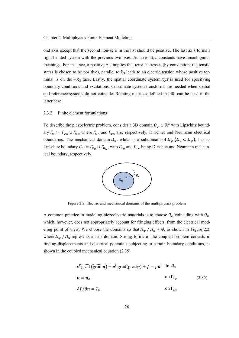
To describe the piezoelectric problem, consider a 3D domain 𝛺 ∈ ℝ with Lipschitz bound-ary 𝛤 ∶= 𝛤 ∪ 𝛤 where 𝛤 and 𝛤 are, respectively, Dirichlet and Neumann electrical boundaries. The mechanical domain Ω , which is a subdomain of 𝛺 𝛺 ⊂ 𝛺 , has its Lipschitz boundary 𝛤 ∶= 𝛤 ∪ 𝛤 , with 𝛤 and 𝛤 being Dirichlet and Neumann mechan-ical boundary, respectively.
Figure 2.2. Electric and mechanical domains of the multiphysics problem
A common practice in modeling piezoelectric materials is to choose 𝛺 coinciding with 𝛺 , which, however, does not appropriately account for fringing effects, from the electrical mod-eling point of view. We choose the domains so that 𝛺 ∕ 𝛺 ≠ ∅, as shown in Figure 2.2. where 𝛺 ∕ 𝛺 represents an air domain. Strong forms of the coupled problem consists in finding displacements and electrical potentials subjecting to certain boundary conditions, as shown in the coupled mechanical equation (2.35)
𝒄 grad grad 𝒖 + 𝒆 grad(grad𝜑) + 𝒇 = 𝜌�̈�
𝒖 = 𝒖
𝜕𝑇 𝜕𝒏⁄ = 𝑇
in Ω
on Γ
on Γ
(2.35)
2.3. Piezoelectric model
27
and the coupled electrostatic equation (2.36)
𝒆 grad grad 𝒖 − 𝜺 grad(grad𝜑) = 0
− 𝜺 grad(grad𝜑) = 0
𝜑 = 𝜑
𝜕𝜑 𝜕𝒏⁄ = 0
in Ω
in Ω ∕ Ω
on Γ
on Γ
(2.36)
where 𝒖 , 𝑇 , and 𝜑 are predefined values for respectively, displacements, surface tractions, and electrical potentials. 𝒏 is the unit outward normal to the boundary. The symbol ‘ ̈ ’ indi-cates second order time derivative.
Meanwhile, electrodes, which are deposited on piezoelectric units, impose equipotential elec-trical conditions. Mechanically, their influences are negligible as they are very thin. Hence, electrodes can be considered as surfaces, involving only equipotential conditions. We address modeling for electrodes and electrical loads after setting up elementary FE systems.
2.3.2.1 Finite element approximations
First, we define some integrals, as presented in Equation (2.37).
𝐵 (𝒖′ , 𝒖) ∶= 𝒖′ 𝒄 grad grad 𝒖 − 𝜌�̈� 𝑑𝛺
𝐵 (𝒖′ , 𝜑) ∶= 𝒖′ 𝒆 grad(grad𝜑) 𝑑𝛺
𝐵 (𝜑 , 𝒖) ≔ 𝜑 𝒆 grad grad 𝒖
𝑑𝛺
𝐵 (𝜑 , 𝜑) ≔ 𝜑 𝜺 grad(grad𝜑)
𝑑𝛺
(𝒖′ , 𝒇) ∶= 𝒖 𝒇 𝑑𝛺, (𝒖′ , 𝑇 ) ≔ 𝒖 𝑇 𝑑𝛤
(2.37)

Chapter 2. Multiphysics Finite Element Modeling
28
Then consider the weak form: find 𝒖 ∈ (𝒰) and 𝜑 ∈ 𝒱 such that
𝐵 (𝒖′ , 𝒖) + 𝐵 (𝒖′ , 𝜑) = −(𝒖′ , 𝒇) + (𝒖′ , 𝑇 ) ∀ 𝒖′ ∈ 𝒰
𝐵 (𝜑′ , 𝜑) + 𝐵 (𝜑′ , 𝒖) = 0 ∀ 𝜑 ∈ 𝒱 (2.38)
In (2.38), 𝒰 and 𝒱 are Hilbert spaces - ℋ(grad, Ω); 𝒰 and 𝒱 are, respectively, subspaces of 𝒰 and 𝒱 subject to boundary conditions. Discrete counterparts of Equation (2.38) read: find 𝒖 ∈ (𝒰 ) and 𝜑 ∈ 𝒱 so that equations in (2.39) hold. In the equation, 𝒰 ⊂ 𝒰, 𝒰 ⊂ 𝒰, 𝒱 ⊂ 𝒱, and 𝒱 ⊂ 𝒱 are finite dimensional subspaces associated with the triangulation, with ℎ characterizing resolution of the latter.
𝐵 (𝒖 ′ , 𝒖 ) + 𝐵 (𝒖 ′ , 𝜑 ) = −(𝒖 ′ , 𝒇) + (𝒖 ′ , 𝑇 ) ∀ 𝒖 ′ ∈ 𝒰
𝐵 (𝜑 ′ , 𝜑 ) + 𝐵 (𝜑 ′ , 𝒖 ) = 0 ∀ 𝜑 ∈ 𝒱 (2.39)
Within an element 𝒦 , the weak form can be build using the Galerkin method, with the trial functions expressed as in Equation (2.40) where 𝑛 is the number of vertices in 𝒦 . 𝜔 are 0-form based nodal basis functions. 𝑢 and 𝜑 are nodal values associated with vertices. Practically, it is more convenient to arrange unknowns in vectors. In this case, entries of 𝒖 i.e. 𝑢 ′s, 𝑗 = 1,2,3 can be written as 𝑈 = [𝑢 𝑣 𝑤 ] in which 𝑢, 𝑣 and 𝑤 are recov-ered from 𝑢 for 𝑖 = 1,2,3.
𝑢 ( ) = 𝜔 𝑢 , 𝜑 ( ) = 𝜔 𝜑 (2.40)
Re-writing (2.40) in compact form gives (2.41).
𝑈 ( ) ∶= 𝑾 , 𝑈 , 𝜑 ( ) ∶= 𝑊 , 𝛷 (2.41)
where 𝑈 ∶= u v w ⋯ w , 𝛷 ∶= 𝜑 𝜑 ⋯ 𝜑 , 𝑾 , ∶= 𝜔 𝑰 𝜔 𝑰 ⋯ 𝜔 𝑰 , 𝑊 , ∶= 𝜔 𝜔 ⋯ 𝜔 , 𝐈 is the third order identity matrix.
2.3. Piezoelectric model
29
𝑴( )�̈� + 𝑲( )𝑈 + 𝑲( )𝛷 = 𝐹 ( )
𝑲( ), 𝑈 − 𝑲( )𝛷 = 0
−𝑲( )𝛷 = 0
for 𝒦 ∈ 𝛺
for 𝒦 ∈ 𝛺 𝛺⁄
(2.42)
Substituting (2.41) into (2.39) leads to elementary systems in (2.42) where 𝑈 , 𝛷 and 𝛷represent, respectively nodal values in the element 𝛷 (associated with piezoelectric materi-als) and element 𝒦 (associated with the air domain). Without losing generality, assume line-ar tetrahedral elements are used for discretization (see e.g. [41] for discussion on other types of elements). The mass matrix 𝑴( ), stiffness matrices 𝑲( ) and 𝑲( ), coupling matrix 𝑲( )
and load vector 𝐹 ( ) are calculated as in (2.43). Superscripts 𝛼 and 𝛽 correspond, respective-ly, to 𝒦 and 𝒦 whereas 𝑡 denotes tensor transpose. 𝑩 and 𝑩 are defined as in (2.44).
𝑴( ) = 𝑾 , , 𝜌𝑾𝒦
𝑑𝛺 , 𝑲( ) = 𝑩 , 𝒄 𝑩𝒦
𝑑𝛺 ,
𝑲( ) = 𝑩 , 𝒆 𝑩𝒦
𝑑𝛺 , 𝑲( / ) = 𝑩 / , 𝜺 𝑩 /
𝒦 /
𝑑𝛺 ,
𝐹 ( ) = 𝑾 , , 𝜌𝒇𝒦
𝑑𝛺 + 𝑾 , , 𝜌𝑡̅∩ 𝒦
𝑑𝛤
(2.43)
𝑩 ∶= [𝑩 𝑩 𝑩 𝑩 ]
𝑩 ∶=
⎣⎢⎢⎢⎢⎢⎡𝜕𝜔
𝜕𝑥𝜕𝜔
𝜕𝑥𝜕𝜔
𝜕𝑦𝜕𝜔
𝜕𝑦𝜕𝜔
𝜕𝑧𝜕𝜔
𝜕𝑧
𝜕𝜔𝜕𝑥
𝜕𝜔𝜕𝑥
𝜕𝜔𝜕𝑦
𝜕𝜔𝜕𝑦
𝜕𝜔𝜕𝑧
𝜕𝜔𝜕𝑧 ⎦
⎥⎥⎥⎥⎥⎤
𝐁 ∶=
⎣⎢⎢⎢⎢⎢⎡∂𝜔
∂𝑥0 0
0∂𝜔
∂𝑦0
0 0∂𝜔
∂𝑧
∂𝜔∂y
0∂𝜔
∂𝑧∂𝜔
∂𝑥∂𝜔
∂𝑧0
0∂𝜔
∂𝑦∂𝜔
x ⎦⎥⎥⎥⎥⎥⎤
(2.44)
Chapter 2. Multiphysics Finite Element Modeling
30
To model structural damping, Rayleigh damping can be considered. It introduces the damping matrix as a fraction of the mass and stiffness matrices using 𝛼 and 𝛽 , as in (2.45). Here, 𝜉 denotes the damping factor at resonant frequency 𝜔 . It can be measured at the first two resonant frequencies with which 𝛼 and 𝛽 are calculated and used for the whole frequen-cy range, approximately [42].
𝑪( ) ∶= 𝛼 𝑴( ) + 𝛽 𝑲( ) , 𝜉 =12
𝛼𝜔
+ 𝛽 𝜔 (2.45)
Adding Equation (2.45) into the first equation of (2.42) yields the elementary system
𝑴( )�̈� + 𝑪( )�̇� + 𝑲( )𝑈 + 𝑲( )𝛷 = 𝐹 ( ) . (2.46)
It is noted that damping also prevents singularity in the frequency regime when the problem is solved near frequencies of resonance. Before assembling elementary matrices into the global system, modeling electrodes and electrical loads are discussed.
2.3.2.2 Modeling the electrodes and electrical loads
Denote the surface of the 𝑘-th electrode as 𝑆 . The equipotential condition means 𝜑(𝑋) =𝜑 for 𝑋 ∈ 𝑆 . When electric potentials are prescribed, this can be realized via Dirichlet boundary conditions. Otherwise, extra treatments are required. Suppose there are 𝑛 vertices on 𝑆 . Then, the number of electrical DoFs is reduced to one for all the 𝑛 nodes. Without losing generality, assume all 𝑛 electrical DoFs are assigned with the numbering 𝑘. If there are 𝑚 electrodes, the total number of electrical DoFs not on electrodes is 𝑛 − ∑ 𝑛 . These DoFs can be numbered from 𝑚 + 1 to 𝑚 + 𝑛 − ∑ 𝑛 − 𝑛 , with 𝑛 denoting the number of nodes on Dirichlet boundaries 𝛤 . For elastic the field, the 𝑗-th component of DoFs associated with the 𝑙-th vertex is numbered as 3 × 𝑙 + 𝑗 − 1 (𝑗 = 1,2,3). Hence, the total number of mechanical and electrical DoFs (denoted by 𝑛 and 𝑛 ) are 3𝑛 − 𝑛 and 𝑚 + 𝑛 − 𝑛 − ∑ 𝑛 (𝑛 number of nodes on 𝛤 ), respectively.
𝑴 �̈� + 𝑪 �̇� + 𝑲 𝑈 + 𝑲 𝛷 = 𝐹
𝑲 𝑈 − 𝑲 𝛷 = 0 (2.47)

2.3. Piezoelectric model
31
After assembling, global systems can be obtained as in (2.47) where 𝑴 , 𝑪 , 𝑲 ∈ ℝ × , 𝑲 ∈ ℝ × ,𝑲 ∈ ℝ × , and 𝐹 ∈ ℝ × . Equations in (2.47) can be transformed from the time regime to the frequency regime. For a time-harmonic excitation at angular fre-quency ω, the transformed system reads
(−𝜔 𝑴 + 𝑗𝜔𝑪 + 𝑲 )𝑈 + 𝑲 𝛷 = 𝐹
𝑲 𝑈 − 𝑲 𝛷 = 0 (2.48)
Incorporating electric circuits can be achieved by using equivalent admittance matrix [43] and modifying the dielectric matrix in the second equation of (2.48). To be more specific, 𝑲 is replaced with 𝑲 + 𝑲 in which the effective capacitance matrix 𝑲 is initially null. For each circuit element 𝑥 connected between the 𝑝-th and 𝑞-th electrode, define a vector 𝑉 that is of size 𝑛 × 1 with the 𝑝-th and 𝑞-th entry being 1 or -1, and others being zero. For con-ciseness, We denote the product 𝑉 𝑉 by 𝑲 . Eventually, − 𝑗 𝜔𝑍⁄ 𝑲 is added to 𝑲 :
𝑲 =𝑗
𝜔𝑍𝑲 . (2.49)
where 𝑍 = −𝑍 when 𝑥 denotes a capacitor, 𝑍 = 𝑍 when 𝑥 denotes a resistor or inductor. 𝑍 is the impedance of 𝑥. The new system can be expressed as in Equation (2.50).
(−𝜔 𝑴 + 𝑗𝜔𝑪 + 𝑲 )𝑈 + 𝑲 𝛷 = 𝐹
𝑲 𝑈 − 𝑲 + 𝑲 𝛷 = 0 (2.50)
In this way, a FE system that considers both electrodes and electrical loads is built. Note that while the final FE formulations are expressed in frequency domain, they can be used for tran-sient analysis (after transferring back to time domain).
2.3.3 Numerical examples
In this part, we present simulations based on the developed model. The first one consists in modal analysis and parametric study of a cantilevered piezoelectric bimorph. The second consists in assessment of thermos-elastic attenuation in SAW device [44].

Chapter 2. Multiphysics Finite Element Modeling
32
2.3.3.1 Cantilevered piezoelectric bimorph
As shown in Figure 2.3, the bimorph is fixed onto a base. In practice, acceleration is applied on the base. For modeling, it is more convenient to consider displacements w.r.t. the base, which means the system is fixed on the base and subject to an acceleration 𝑎(𝑓).
Figure 2.3. The cantilevered bimorph. (a) model configuration, (b) triangulation
Dimensions of the bimorph are set, so that piezoelectric layers are of 27 × 3.2 × 0.258 𝑚𝑚whereas the substrate in sandwiched by piezoelectric layers is of 27 × 3.2 × 0.115 𝑚𝑚 .Meanwhile, we suppose that electrodes are connected in series (though little work is required for the case of a parallel connection) [45]. Piezoelectric layers are made of PZT-5H, while the substrate is made of brass. Material constants are summarized in Table 2.2.
To perform modal analysis, (2.50) is re-formulated as
(−𝜔 𝑴 + 𝑗𝜔𝑪 + 𝑲)𝑋 = 𝐹 (2.51)
where 𝑋 = [𝑈, 𝛷] whereas 𝑴, 𝑪, and 𝑲 comprise corresponding elastic and electrical terms.
The problem amounts to setting 𝐹 to zero and solving the Eigen problem for resonant fre-quencies 𝜔 and vibration mode shapes 𝑋. It is noted that instead of solving a purely structural
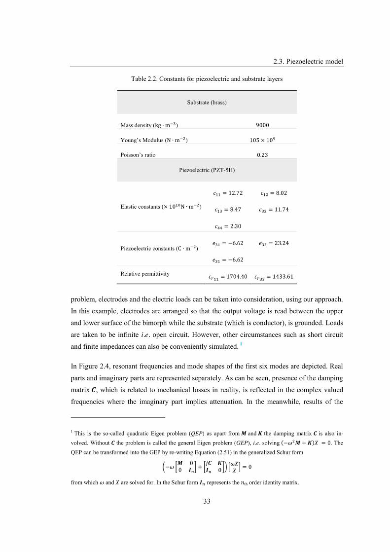
2.3. Piezoelectric model
33
Table 2.2. Constants for piezoelectric and substrate layers
Substrate (brass)
Mass density (kg ∙ m ) 9000
Young’s Modulus (N ∙ m ) 105 × 10
Poisson’s ratio 0.23
Piezoelectric (PZT-5H)
Elastic constants (× 10 N ∙ m )
𝑐 = 12.72 𝑐 = 8.02
𝑐 = 8.47 𝑐 = 11.74
𝑐 = 2.30
Piezoelectric constants (C ∙ m )𝑒 = −6.62 𝑒 = 23.24
𝑒 = −6.62
Relative permittivity 𝜀 = 1704.40 𝜀 = 1433.61
problem, electrodes and the electric loads can be taken into consideration, using our approach. In this example, electrodes are arranged so that the output voltage is read between the upper and lower surface of the bimorph while the substrate (which is conductor), is grounded. Loads are taken to be infinite i.e. open circuit. However, other circumstances such as short circuit and finite impedances can also be conveniently simulated. 1
In Figure 2.4, resonant frequencies and mode shapes of the first six modes are depicted. Real parts and imaginary parts are represented separately. As can be seen, presence of the damping matrix 𝑪, which is related to mechanical losses in reality, is reflected in the complex valued frequencies where the imaginary part implies attenuation. In the meanwhile, results of the
1 This is the so-called quadratic Eigen problem (QEP) as apart from 𝑴 and 𝑲 the damping matrix 𝑪 is also in-volved. Without 𝑪 the problem is called the general Eigen problem (GEP), i.e. solving (−𝜔 𝑴 + 𝑲)𝑋 = 0. TheQEP can be transformed into the GEP by re-writing Equation (2.51) in the generalized Schur form
−𝜔 𝑴 00 𝑰 + 𝑗𝑪 𝑲
𝑰 0𝜔𝑋𝑋 = 0
from which 𝜔 and 𝑋 are solved for. In the Schur form 𝑰 represents the 𝑛th order identity matrix.
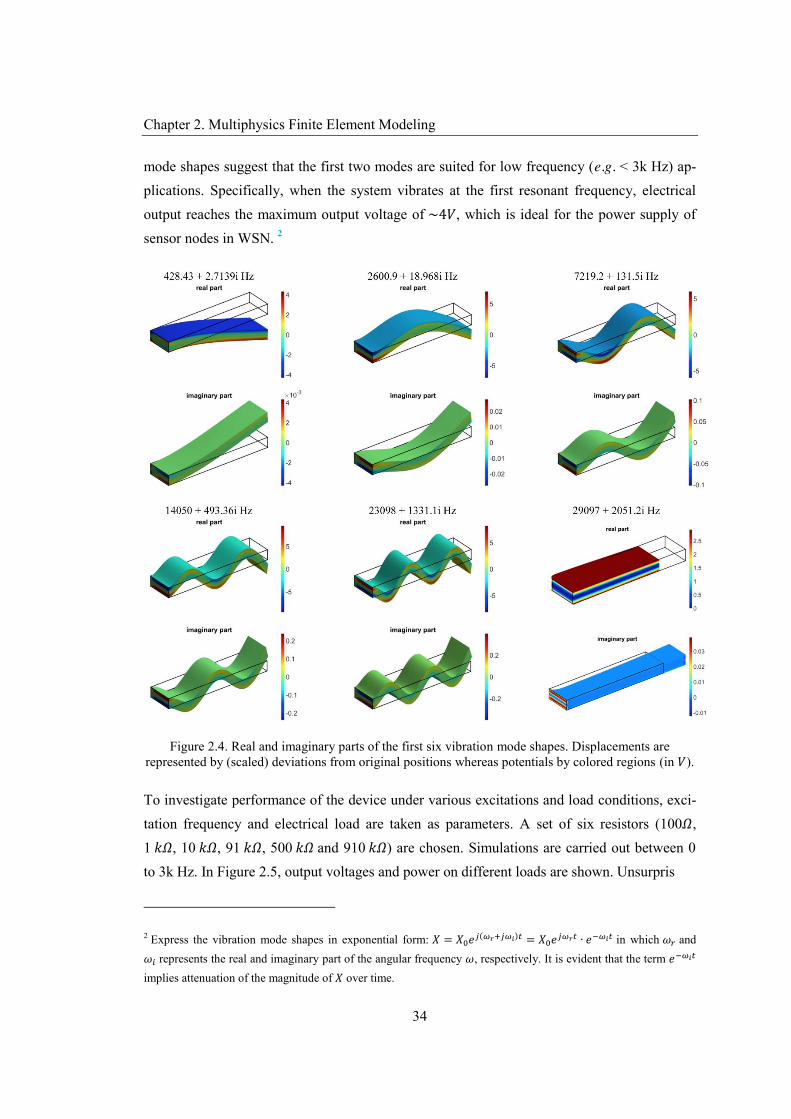
Chapter 2. Multiphysics Finite Element Modeling
34
mode shapes suggest that the first two modes are suited for low frequency (e.g. < 3k Hz) ap-plications. Specifically, when the system vibrates at the first resonant frequency, electrical output reaches the maximum output voltage of ~4𝑉, which is ideal for the power supply of sensor nodes in WSN. 2
Figure 2.4. Real and imaginary parts of the first six vibration mode shapes. Displacements are represented by (scaled) deviations from original positions whereas potentials by colored regions (in 𝑉).
To investigate performance of the device under various excitations and load conditions, exci-tation frequency and electrical load are taken as parameters. A set of six resistors (100𝛺, 1 𝑘𝛺, 10 𝑘𝛺, 91 𝑘𝛺, 500 𝑘𝛺 and 910 𝑘𝛺) are chosen. Simulations are carried out between 0 to 3k Hz. In Figure 2.5, output voltages and power on different loads are shown. Unsurpris
2 Express the vibration mode shapes in exponential form: 𝑋 = 𝑋 𝑒 ( ) = 𝑋 𝑒 ∙ 𝑒 in which 𝜔 and𝜔 represents the real and imaginary part of the angular frequency 𝜔, respectively. It is evident that the term 𝑒implies attenuation of the magnitude of 𝑋 over time.
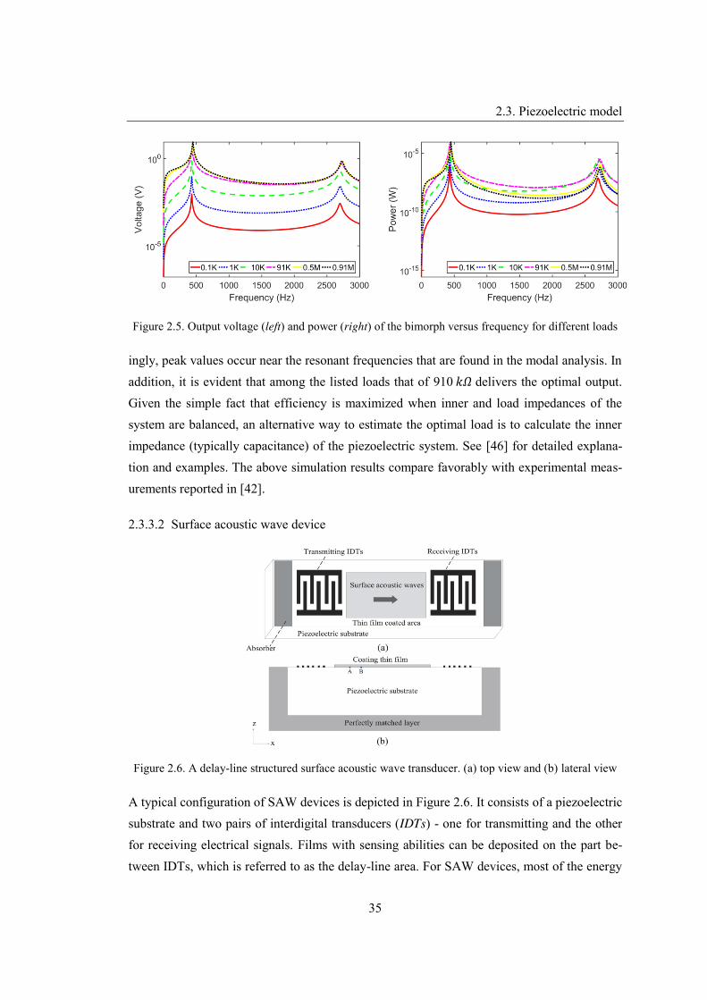
2.3. Piezoelectric model
35
Figure 2.5. Output voltage (left) and power (right) of the bimorph versus frequency for different loads
ingly, peak values occur near the resonant frequencies that are found in the modal analysis. In addition, it is evident that among the listed loads that of 910 𝑘𝛺 delivers the optimal output. Given the simple fact that efficiency is maximized when inner and load impedances of the system are balanced, an alternative way to estimate the optimal load is to calculate the inner impedance (typically capacitance) of the piezoelectric system. See [46] for detailed explana-tion and examples. The above simulation results compare favorably with experimental meas-urements reported in [42].
2.3.3.2 Surface acoustic wave device
Figure 2.6. A delay-line structured surface acoustic wave transducer. (a) top view and (b) lateral view
A typical configuration of SAW devices is depicted in Figure 2.6. It consists of a piezoelectric substrate and two pairs of interdigital transducers (IDTs) - one for transmitting and the other for receiving electrical signals. Films with sensing abilities can be deposited on the part be-tween IDTs, which is referred to as the delay-line area. For SAW devices, most of the energy
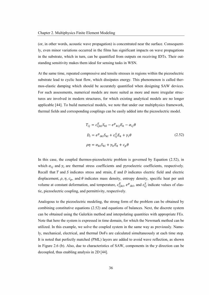
Chapter 2. Multiphysics Finite Element Modeling
36
(or, in other words, acoustic wave propagation) is concentrated near the surface. Consequent-ly, even minor variations occurred in the films has significant impacts on wave propagations in the substrate, which in turn, can be quantified from outputs on receiving IDTs. Their out-standing sensitivity makes them ideal for sensing tasks in WSN.
At the same time, repeated compressive and tensile stresses in regions within the piezoelectric substrate lead to cyclic heat flow, which dissipates energy. This phenomenon is called ther-mos-elastic damping which should be accurately quantified when designing SAW devices. For such assessments, numerical models are more suited as more and more irregular struc-tures are involved in modern structures, for which existing analytical models are no longer applicable [44]. To build numerical models, we note that under our multiphysics framework, thermal fields and corresponding couplings can be easily added into the piezoelectric model.
𝑇 = 𝑐 𝑆 − 𝑒 𝐸 − 𝛼 𝜃
𝐷 = 𝑒 𝑆 + 𝜀 𝐸 + 𝛾 𝜃
𝜌𝜂 = 𝛼 𝑆 + 𝛾 𝐸 + 𝑐 𝜃
(2.52)
In this case, the coupled thermos-piezoelectric problem is governed by Equation (2.52), in which 𝛼 and 𝛾 are thermal stress coefficients and pyroelectric coefficients, respectively.Recall that 𝑇 and 𝑆 indicates stress and strain, 𝐸 and 𝐷 indicates electric field and electric displacement, 𝜌, 𝜂, 𝑐 , and 𝜃 indicates mass density, entropy density, specific heat per unitvolume at constant deformation, and temperature, 𝑐 , 𝑒 , and 𝜀 indicate values of elas-tic, piezoelectric coupling, and permittivity, respectively.
Analogous to the piezoelectric modeling, the strong form of the problem can be obtained by combining constitutive equations (2.52) and equations of balances. Next, the discrete system can be obtained using the Galerkin method and interpolating quantities with appropriate FEs. Note that here the system is expressed in time domain, for which the Newmark method can be utilized. In this example, we solve the coupled system in the same way as previously. Name-ly, mechanical, electrical, and thermal DoFs are calculated simultaneously at each time step. It is noted that perfectly matched (PML) layers are added to avoid wave reflection, as shown in Figure 2.6 (b). Also, due to characteristics of SAW, components in the 𝑦 direction can be decoupled, thus enabling analysis in 2D [44].

2.3. Piezoelectric model
37
Figure 2.7. Displacements in the 𝑧 direction of points A and B
A 2D model is built for the thermos-piezoelectric problem. Simulations are carried out for both coated and uncoated conditions (that corresponds to the case with or without the pres-ence of the film in Figure 2.6 (b), respectively). Regarding the model set-up, we use a 𝑌- cut LiNbO3 (see [44] for constant values of the material) substrate of 30𝜆 × 10 𝜆 (where 𝜆 is the wavelength at a central frequency 𝑓 of 300 𝑀𝐻𝑧). A total of 24 electrodes are modeled in IDTs. Meanwhile, relatively fine meshes (with maximum element length of 1 32⁄ 𝜆) and small time steps (of 0.025 𝑓⁄ ) are chosen so as to ensure accuracy of the results.
Figure 2.8. Wave amplitude versus propagation distance (attenuation proportional to slopes of the lines)
In Figure 2.7 displacements in the 𝑧 direction at two points 𝐴 and 𝐵 (as marked in Figure 2.6) are depicted. Point 𝐴 is closer to transmitting IDTs, sitting four wavelength away from point 𝐵. Displacements at both points oscillate at constant amplitudes eventually. However, due to thermos-elastic damping slight descending in the amplitude at 𝐵, w.r.t. that at 𝐴 can be ob-served. Both simulated and reference results [47] in terms of wave attenuation are presented in Figure 2.8. As the figure implies, excellent correlations are obtained.
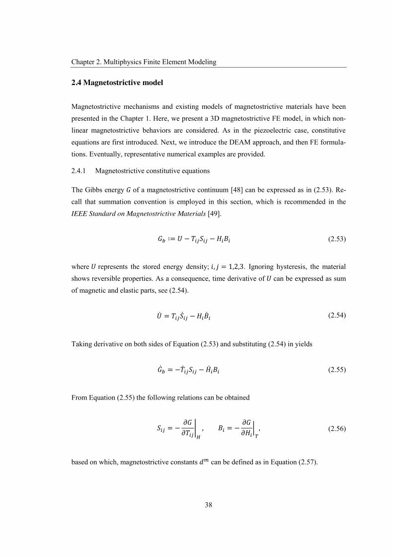
Chapter 2. Multiphysics Finite Element Modeling
38
2.4 Magnetostrictive model
Magnetostrictive mechanisms and existing models of magnetostrictive materials have been presented in the Chapter 1. Here, we present a 3D magnetostrictive FE model, in which non-linear magnetostrictive behaviors are considered. As in the piezoelectric case, constitutive equations are first introduced. Next, we introduce the DEAM approach, and then FE formula-tions. Eventually, representative numerical examples are provided.
2.4.1 Magnetostrictive constitutive equations
The Gibbs energy 𝐺 of a magnetostrictive continuum [48] can be expressed as in (2.53). Re-call that summation convention is employed in this section, which is recommended in the IEEE Standard on Magnetostrictive Materials [49].
𝐺 ∶= 𝑈 − 𝑇 𝑆 − 𝐻 𝐵 (2.53)
where 𝑈 represents the stored energy density; 𝑖, 𝑗 = 1,2,3. Ignoring hysteresis, the material shows reversible properties. As a consequence, time derivative of 𝑈 can be expressed as sum of magnetic and elastic parts, see (2.54).
�̇� = 𝑇 �̇� − 𝐻 �̇� (2.54)
Taking derivative on both sides of Equation (2.53) and substituting (2.54) in yields
�̇� = −�̇� 𝑆 − �̇� 𝐵 (2.55)
From Equation (2.55) the following relations can be obtained
𝑆 = −𝜕𝐺
𝜕𝑇, 𝐵 = −
𝜕𝐺𝜕𝐻
, (2.56)
based on which, magnetostrictive constants 𝑑 can be defined as in Equation (2.57).

2.4. Magnetostrictive model
39
𝑑 =𝜕𝑆𝜕𝐻
=𝜕𝐵𝜕𝑇 (2.57)
As the equation suggests, 𝑑 denotes derivatives of strain (respectively, magnetic flux densi-ty) w.r.t. magnetic field (respectively, stress), under constant stress (respectively, magnetic field). Given the relations between (𝑆, 𝐵) and (𝑇, 𝐻), magnetostrictive constitutive equations can be obtained as in (2.58) where superscripts 𝐻 in 𝑠 and 𝑇 in 𝜇 indicates values ofcompliance and permeability, under constant magnetic field and stress, respectively.
𝛿𝑆 = 𝑠 𝛿𝑇 + 𝑑 𝛿𝐻
𝛿𝐵 = 𝑑 𝛿𝑇 + 𝜇 𝛿𝐻(2.58)
For FE modeling, it is more convenient to express (𝑇, 𝐻) in terms of (𝑆, 𝐵), as expressed in (2.59) where magnetostrictive constants ℎ(𝑁 ∙ 𝑊𝑏 𝑜𝑟 𝐴 ∙ 𝑚 ) instead of 𝑑 (𝑊𝑏 ∙𝑁 , or 𝑚 ∙ 𝐴 ) are used; 𝜈 (𝑚 ∙ 𝐻 𝑜𝑟 4π. 10 𝑂𝑒 ∙ 𝐺 ) indicates reluctivity under con-stant strain. In literature, 𝐵 may be expressed in either 𝐺 or 𝑇 (1𝑇 = 10 𝐺), while 𝐻 may beexpressed in either 𝐴 ∙ 𝑚 or 𝑂𝑒 (1𝐴 ∙ 𝑚 = 4π. 10 𝑂𝑒) . Other forms of constitutiveequations, as well as conversions between different sets of constants, are addressed in [49].
𝛿𝑇 = 𝑐 𝛿𝑆 − ℎ 𝛿𝐵
𝛿𝐻 = −ℎ 𝛿𝑆 + 𝜈 𝛿𝐵(2.59)
In (2.59), 𝛿 implies quantities of perturbation. When deviations in equations in (2.59) are small enough, the linear form can be obtained, see (2.60).
𝑇 = 𝑐 𝑆 − ℎ 𝐵
𝐻 = −ℎ 𝑆 + 𝜈 𝐵(2.60)
2.4.2 The discrete energy averaged model
DEAM was first introduced for modeling Galfenol, and later adopted for modeling Terfenol-

Chapter 2. Multiphysics Finite Element Modeling
40
D. Exceptional correlations between DEAM based simulation results and experimental meas-urements are reported, see [50], [17], [18], and [19]. We implemented it on a C++ platform. The program is compiled as a mex file that can be called from MATLAB programs directly (for integration with FE programs, as the latter are implemented on MATLAB).
For DEAM, it is assumed that magnetostrictive materials are composed by non-interacting, single-domain particles whose magnetocrystalline anisotropy gives domains easy directions (denoted by 𝒄 ). When the material undergoes variation of magnetic fields 𝐻 and stresses 𝑇, these single-domains tend to rotate, and align themselves along the orientation 𝒎 . The bulk magnetization 𝑀 and magnetostriction 𝑆 are obtained as the weighted sum of the magnetiza-tion 𝑀 𝒎 (with 𝑀 representing the saturation magnetization) and magnetostriction 𝑆 from each orientation, as expressed in Equation (2.61). Note that strain 𝑆 is assumed to be decom-posed into magnetostriction 𝑆 and a purely mechanical part 𝑆 (determined by stresses).
𝑀 = 𝜉 𝑀 𝒎 , 𝑆 = 𝜉 𝑆 (2.61)
where 𝜉 is the averaged hysteretic volume fractions of the particle, calculated as energy-weighted averages, see Equation (2.62).
𝜉 ∶= exp − 𝐺 Ω⁄ ∙ exp 𝐺 Ω⁄ (2.62)
In(2.62) Ω is the Armstrong smoothing factor, whereas 𝐺 is the Gibbs free energy - the sum of anisotropy, coupling and the Zeeman energy, corresponding to the first, second and third term on the r.h.s. of (2.63), respectively. 𝐾 is the anisotropy coefficient.
𝐺 ∶=12
𝐾 𝒎 − 𝒄 − 𝑆 ∙ 𝑇 − 𝜇 𝑀 𝒎 ∙ 𝐻 (2.63)
Denote entries of 𝒎 as 𝑚 with 𝑖 = 1,2,3. For particles with cubic symmetry, magneto-striction 𝑆 in 𝒎 direction can be expressed as in Equation (2.64) where 𝑐 and 𝑐 are elastic moduli, while 𝜆 and 𝜆 are magnetostriction constants.
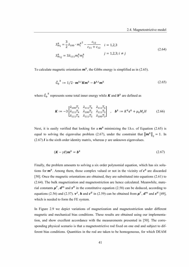
2.4. Magnetostrictive model
41
𝑆 =
32
𝜆 ∙ 𝑚 −𝑐
𝑐 + 𝑐
𝑆 = 3𝜆 𝑚 𝑚
𝑖 = 1,2,3
𝑗 = 1,2,3; 𝑖 ≠ 𝑗 (2.64)
To calculate magnetic orientation 𝒎 , the Gibbs energy is simplified as in (2.65).
𝐺 ∶= 1 2⁄ ∙ 𝒎 , 𝑲𝒎 − 𝒃 , 𝒎 (2.65)
where 𝐺 represents some total inner energy while 𝑲 and 𝒃 are defined as
𝑲 ∶= −3𝜆 𝑇 𝜆 𝑇 𝜆 𝑇𝜆 𝑇 𝜆 𝑇 𝜆 𝑇𝜆 𝑇 𝜆 𝑇 𝜆 𝑇
, 𝒃 ∶= 𝐾 𝒄 + 𝜇 𝑀 𝐻 (2.66)
Next, it is easily verified that looking for a 𝒎 minimizing the l.h.s. of Equation (2.65) is equal to solving the eigenvalue problem (2.67), under the constraint that 𝒎 = 1. In (2.67) 𝑰 is the sixth order identity matrix, whereas 𝛾 are unknown eigenvalues.
(𝑲 − 𝛾𝑰)𝒎 = 𝒃 (2.67)
Finally, the problem amounts to solving a six order polynomial equation, which has six solu-tions for 𝒎 . Among them, those complex valued or not in the vicinity of 𝒄 are discarded [50]. Once the magnetic orientations are obtained, they are substituted into equations (2.61) to (2.64). The bulk magnetization and magnetostriction are hence calculated. Meanwhile, mate-rial constants 𝝁 , 𝒅 and 𝒔 in the constitutive equation (2.58) can be deduced, according to equations (2.56) and (2.57). 𝝂 , 𝒉 and 𝒄 in (2.59) can be obtained from 𝝁 , 𝒅 and 𝒔 [49], which is needed to form the FE system.
In Figure 2.9 we depict variations of magnetization and magnetostriction under different magnetic and mechanical bias conditions. These results are obtained using our implementa-tion, and show excellent accordance with the measurements presented in [50]. The corre-sponding physical scenario is that a magnetostrictive rod fixed on one end and subject to dif-ferent bias conditions. Quantities in the rod are taken to be homogeneous, for which DEAM

Chapter 2. Multiphysics Finite Element Modeling
42
needs to be run only once for a given combination of state variables (namely, the aforemen-tioned macroscopic and microscopic volumes refer to the same thing - the rod itself; the case of non-homogeneity i.e. the number of microscopic volumes is larger than the macroscopic one is discussed in § 2.4.4.3).
Figure 2.9. Simulation results of nonhysteretic magnetization (right) and magnetostriction (left) for ⟨100⟩𝐹𝑒 . 𝐺𝑎 . at various stress (top) and field (bottom) values
2.4.3 Finite element formulations
Figure 2.10. Domains of the magnetostrictive problem
To formulate the magnetostrictive problem, consider a domain Ω ∈ ℝ that is composed bysubdomains Ω , Ω , and Ω , representing the air, support of source currents and magneto-strictive materials, respectively (see Figure 2.10). Note that here we consider the effect of non-vanishing electric conductivity of magnetostrictive materials, hence Ω can also be inter-preted as the domain of conductors. Also, we ignore eddy currents in the support of source currents. Therefore, Ω can be viewed as part of Ω except that source currents, if there are
2.4. Magnetostrictive model
43
any, are nonzero in Ω while vanishing in other parts of Ω . For textual simplification, Ω will only be mentioned for specification of source currents.
In what below low frequencies operating regimes are assumed, and thus the electric dis-placement term in the Maxwell-Ampère’s theorem is neglected. As a result, magnetic part of the coupled problem (that is the magneto-quasistatic problem) can be represented by (2.68), in which 𝐽 is the imposed source current; 𝜎 𝐸 is the eddy current induced. 𝜎 is nonzero in Ω and vanishing in others.
curl𝐻 = 𝜎 𝐸 + 𝐽
𝜕𝐵 𝜕𝑡⁄ + curl𝐸 = 0 (2.68)
We also assume Ω is sufficiently large so that null boundary conditions on 𝜕Ω are valid. Next, the magnetic vector potential 𝐴 and a scalar potential 𝜙 (which is the primitive of the aforementioned electric potential 𝜑), are introduced so that
𝐵 = curl𝐴
𝐸 = − 𝜕(𝐴 + grad𝜙) 𝜕𝑡⁄ (2.69)
where the negative sign in the second equation is used for symmetry of the discrete system. Substituting Equation (2.69) into (2.68) yields (2.70).
curl(𝝂 ∙ curl𝐴) + 𝜕(𝜎 𝐴 + 𝜎 grad𝜙) 𝜕𝑡⁄ = 𝐽
div(𝐽 − 𝜎 𝜕(𝐴 + grad𝜙) 𝜕𝑡⁄ ) = 0 (2.70)
where the second equation comes from the divergence-free property of the current density. In fact, it can be obtained by taking divergence of both sides of the first equations.
curl𝒯 curl𝒯𝑑Ω = curl𝒯 𝐽 𝑑Ω (2.71)
To explicitly enforce the divergence-free property of 𝐽 , Equation (2.71) is first resolved.

Chapter 2. Multiphysics Finite Element Modeling
44
Therefore, 𝐽 is expressed as curl𝒯 in which 𝒯 is discretized using edge elements 𝜔 , having boundary condition 𝒯 × 𝒏 = 0 on 𝜕Ω. Here 𝒏 denotes the outward unit normal vector.
For magnetostrictive materials, a term corresponding to the magneto-elastic coupling needs to be added into (2.70). That being said, the coupled magnetic problem can be stated as: find 𝐴 ∈ ℋ(curl, Ω) and 𝜙 ∈ ℋ(grad, Ω) such that equations in (2.72) holds true for all 𝐴′ ∈ℋ (curl, Ω) and 𝜙′ ∈ ℋ (grad, Ω). Here, ℋ indicates Hilbert spaces with boundary condi-tions 𝐴 = 0 on 𝜕Ω and 𝜙 = 0 on 𝜕Ω.
curl𝐴 ∙ 𝝂 ∙ curl𝐴 𝑑Ω − curl𝐴 ∙ 𝒯𝑑Ω = 0
curl𝐴 ∙ 𝝂 ∙ curl𝐴𝑑Ω − curl𝐴 ∙ 𝒉 ∙ grad𝒖 𝑑Ω
+ 𝜎 𝐴′ ∙ �̇� 𝑑Ω + 𝜎 𝐴′ ∙ grad�̇�𝑑Ω − curl𝐴 ∙ 𝒯𝑑Ω = 0
𝜎 grad𝜙 ∙ �̇� 𝑑Ω + 𝜎 grad𝜙 ∙ grad�̇� 𝑑Ω = 0
in Ω
in Ω
in Ω
(2.72)
In (2.72) 𝒖 represents the mechanical displacement. The standard form is expressed in (2.73).
𝐵 (𝐴 , 𝐴) − 𝐵 (𝐴 , 𝒯) = 0
𝐵 (𝐴 , 𝐴) − 𝐵 (𝐴 , 𝒖) + 𝐶 𝐴 , �̇� + 𝐶 𝐴 , �̇� − 𝐵 (𝐴 , 𝒯) = 0 .
𝐶 𝜙 , �̇� + 𝐵 𝜙 , �̇� = 0
(2.73)
In the meanwhile, the coupled mechanical problem can be represented as in (2.74), which is treated the same way as in the piezoelectric case of previous section,
𝒖 ∙ 𝜌 ∙ �̈� 𝑑Ω + grad𝒖′ ∙ 𝒄 ∙ grad𝒖 𝑑Ω − grad𝒖′ ∙ 𝒉 ∙ curl𝐴 𝑑Ω
+ 𝒖 ∙ 𝒇 𝑑Ω − 𝒖 ∙ �̅� 𝑑Ω = 0 (2.74)
2.4. Magnetostrictive model
45
where 𝑢 ∈ ℋ (grad, Ω). associated boundary conditions are 𝑢 = 𝑢 on Γ and 𝑛 𝑇 = 𝑡on Γ . Appropriate initial conditions are also needed. The standard form corresponding toEquation (2.74) reads
𝑀 (𝒖 , �̈�) + 𝐾 (𝒖 , 𝒖) − 𝐾 (𝒖 , 𝐴) + (𝒖 , 𝒇 ) − (𝒖 , 𝒕 ) = 0 (2.75)
In the above equation, a structural damping term is needed when damping effects are consid-ered. The discrete version of the above weak formulations is presented in (2.76).
𝐵 (𝐴 , 𝐴 ) − 𝐵 (𝐴 , 𝒯 ) = 0
𝐵 (𝐴 , 𝐴 ) − 𝐵 (𝐴 , 𝒖 ) + 𝐶 𝐴 , �̇� + 𝐶 𝐴 , �̇� − 𝐵 (𝐴 , 𝒯 ) = 0
𝐶 𝜙 , �̇� + 𝐵 𝜙 , �̇� = 0
𝑀 (𝒖 , �̈� ) + 𝐵 (𝒖 , 𝒖 ) − 𝐵 (𝒖 , 𝐴 ) + 𝒖 , 𝒇 , − (𝒖 , 𝒕 ) = 0
(2.76)
Variables related to 𝒖 and 𝜙 are interpolants of nodal elements 𝜔 , whereas those related to𝒯 and 𝐴 are interpolants of edge elements 𝜔 . Body forces and surface tractions, if there areany, can be treated the same way as displacements. Substituting the interpolants into (2.76) and using the Galerkin method, we can have (2.77) for elements 𝒦 ∈ Ω and 𝒦 ∈ Ω .
𝑲( )�̅� = 𝐹( )
𝑲( )�̅� − 𝑲( )𝑈 + 𝑪( )�̅̇� + 𝑪( )Ψ̇ = 𝐹( )
𝑪( ), �̅̇� + 𝑲( )Ψ̇ = 0
𝑴( )�̈� + 𝑲( )𝑈 − 𝑲( ), �̅� = 𝐹 ( )
(2.77)
In (2.77), 𝐹( , ) and 𝐹 ( ) are force vectors, whereas �̅� , , 𝑈 , and Ψ̇ represent discretevalues for respectively, 𝐴, 𝒖, and 𝜙. The bar in �̅� , is used to suggest that values are in factline integrals. Recall that the exterior derivative of a 𝑝-form lies in a subspace of the space of (𝑝 + 1)-form, see Equation (2.10). Applying this rule to e.g. curl𝐴 and grad�̇� in Equation
Chapter 2. Multiphysics Finite Element Modeling
46
(2.72), the following identities can be obtained
curl𝐴( ) = curl 𝜔 �̅� = 𝑾 𝑪( )�̅�
grad�̇�( ) = grad 𝜔 �̇� = 𝑾 𝑮( )Ψ
(2.78)
Recall that 𝜔 , 𝜔 , and 𝜔 are nodal, edge, and facet basis functions in 𝒦 (which reads,respectively, 𝑊 , 𝑾 , and 𝑾 , in compact form); 𝑛 , 𝑛 , and 𝑛 are numbers of correspond-ing basis functions; incident matrices associated with discrete gradient, curl, and divergence are denoted by 𝑮, 𝑪, and 𝑫, respectively. Implementations of incident matrices are specified in § A.3. Meanwhile 𝑲( / ), 𝐹( / ), 𝑲( ), 𝑪( ), 𝑪( ) and 𝑲( ) in (2.77) are calculated as in(2.79). Those associated with the elastic problem are treated as in the piezoelectric case, see Equation (2.43).
𝑲 ,( / ) ∶= 𝑪( / ), 𝑾 /
, ∙ 𝝂 ∙ 𝑾 / 𝑑Ω𝒦 ,
𝑪( / )
𝑲( ) ∶= 𝑪( ), 𝑾 ,, ∙ 𝒉 ∙ 𝑩 𝑑Ω
𝒦 ,
𝑪( ) ∶= 𝑾 , 𝜎 𝑾 𝑑Ω𝒦
𝑪( ) ∶= 𝑾 , 𝜎 𝑾 𝑑Ω𝒦
𝑮( )
𝑲( ) ∶= 𝑮( ), 𝑾 , 𝜎 𝑾 𝑑Ω𝒦
𝑮( )
𝐹( / ) ∶= 𝑪( / ), 𝑾 /, ∙ 𝑾 / 𝑑Ω
𝒦𝒯 /
(2.79)
The elementary systems are assembled according to the numbering of elements. The global system is expressed in (2.80).

2.4. Magnetostrictive model
47
𝑲( )�̅� = 𝐹( )
𝑲( )�̅� − 𝑲( )𝑈 + 𝑪( )�̅̇� + 𝑪( )Ψ̇ = 𝐹( )
𝑪( ), �̅̇� + 𝑲( )Ψ̇ = 0
𝑴( )�̈� + 𝑪( )�̇� + 𝑲( )𝑈 − 𝑲( ), �̅� = 𝐹 ( )
(2.80)
Note that in (2.80) superscripts C and D are used to represent, respectively, domains related to magnetostrictive materials and air, similar to those in (2.77) for elementary systems. Also, the damping matrix, generated using the Rayleigh damping, is added to the fourth equation.
2.4.4 Numerical examples
Now, we present three numerical examples that are carried out using our magnetostrictive model. For the first one, magnetic fields are calculated for given source currents, while for the others source currents are set to zero and magnetic fields are obtained for given boundary conditions. The well-known TEAM (Testing Electromagnetic Analysis Methods) Problem 7 is utilized in the first example; the other two examples are concerned with investigation on a cantilevered magnetostrictive unimorph. More precisely, the second example deals with a linear problem whereas the third with a nonlinear one in which we also introduce elaborating DEAM into the FE model.
2.4.4.1 The TEAM Problem 7 (asymmetrical conductor with a hole)
Figure 2.11. Configuration of the TEAM Problem 7
The problem (as shown in Figure 2.11) consist in calculating non-uniform magnetic fields (that are stimulated by a harmonically time varying source current in the coil), and eddy cur-rent in a conductor plate that is placed eccentrically under the coil.
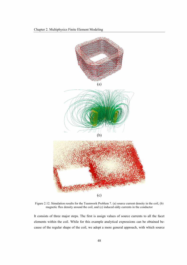
Chapter 2. Multiphysics Finite Element Modeling
48
Figure 2.12. Simulation results for the Teamwork Problem 7. (a) source current density in the coil, (b) magnetic flux density around the coil, and (c) induced eddy currents in the conductor
It consists of three major steps. The first is assign values of source currents to all the facet elements within the coil. While for this example analytical expressions can be obtained be-cause of the regular shape of the coil, we adopt a more general approach, with which source
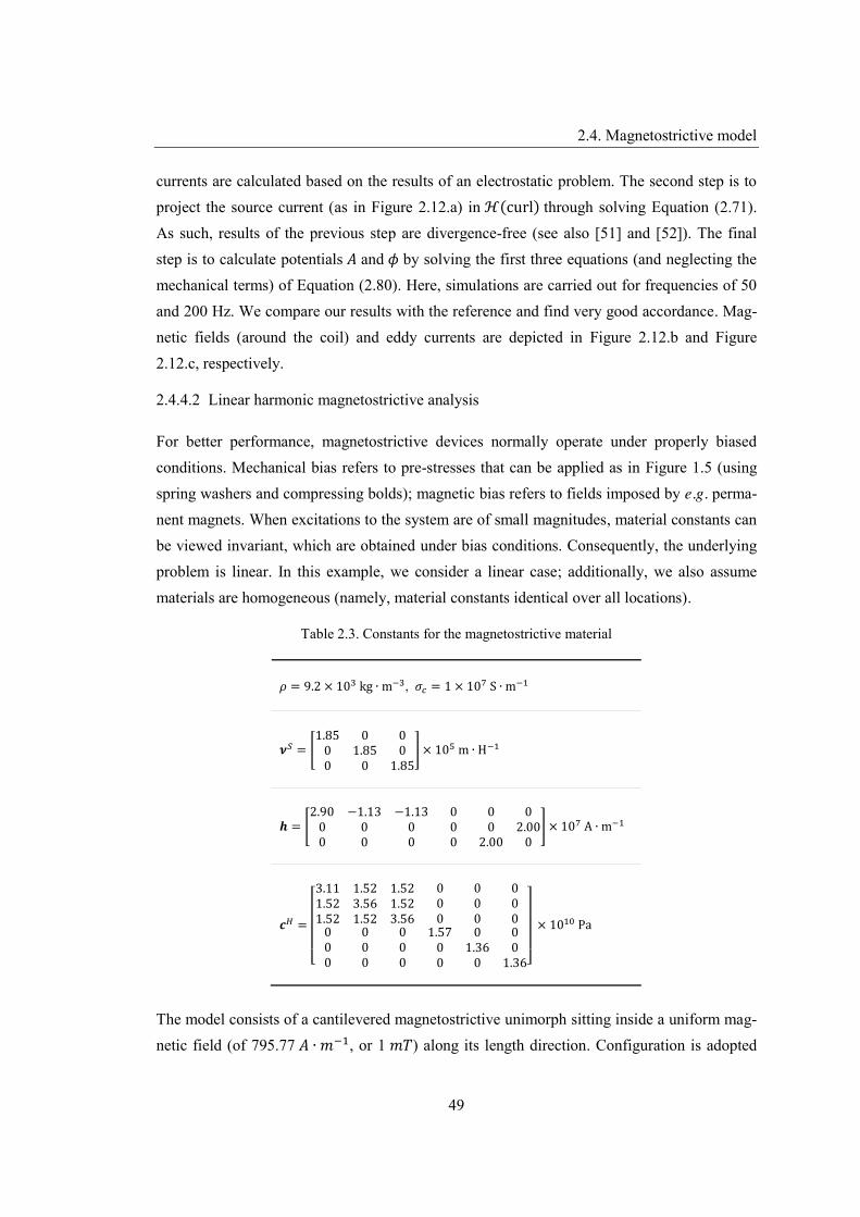
2.4. Magnetostrictive model
49
currents are calculated based on the results of an electrostatic problem. The second step is to project the source current (as in Figure 2.12.a) in ℋ(curl) through solving Equation (2.71). As such, results of the previous step are divergence-free (see also [51] and [52]). The final step is to calculate potentials 𝐴 and 𝜙 by solving the first three equations (and neglecting the mechanical terms) of Equation (2.80). Here, simulations are carried out for frequencies of 50 and 200 Hz. We compare our results with the reference and find very good accordance. Mag-netic fields (around the coil) and eddy currents are depicted in Figure 2.12.b and Figure 2.12.c, respectively.
2.4.4.2 Linear harmonic magnetostrictive analysis
For better performance, magnetostrictive devices normally operate under properly biased conditions. Mechanical bias refers to pre-stresses that can be applied as in Figure 1.5 (using spring washers and compressing bolds); magnetic bias refers to fields imposed by e.g. perma-nent magnets. When excitations to the system are of small magnitudes, material constants can be viewed invariant, which are obtained under bias conditions. Consequently, the underlying problem is linear. In this example, we consider a linear case; additionally, we also assume materials are homogeneous (namely, material constants identical over all locations).
Table 2.3. Constants for the magnetostrictive material
𝜌 = 9.2 × 10 kg ∙ m , 𝜎 = 1 × 10 S ∙ m
𝝂 =1.85 0 0 0 1.85 0 0 0 1.85
× 10 m ∙ H
𝒉 =2.90 −1.13 −1.13 0 0 0 0 0 0
0 0 0 0 0 2.00 0 2.00 0
× 10 A ∙ m
𝒄 =
⎣⎢⎢⎢⎢⎡3.11 1.52 1.521.52 3.56 1.521.52 1.52 3.56
0 0 0 0 0 0 0 0 0
0 0 0 0 0 0 0 0 0
1.57 0 0 0 1.36 0 0 0 1.36⎦
⎥⎥⎥⎥⎤
× 10 Pa
The model consists of a cantilevered magnetostrictive unimorph sitting inside a uniform mag-netic field (of 795.77 𝐴 ∙ 𝑚 , or 1 𝑚𝑇) along its length direction. Configuration is adopted

Chapter 2. Multiphysics Finite Element Modeling
50
from [53], in which dimensions are 5 × 1 × 0.5 𝑚𝑚 , the excitation frequency is 1 𝑘𝐻𝑧(harmonic excitations assumed), material constants are presented in Table 2.2. In addition, we add a sufficiently large air domain around the unimorph, as depicted in Figure 2.13.b.
Figure 2.13. Rsults of the linear magnetostrictive problem (coordinates along the length direction are scaled for representation purpose). (a) edges on which nonzero Dirichlet boundary conditions for 𝐴 are applied; (b) solution of the problem in which arrows depict the magnetic flux distribution whereas the rainbow colored region depicts mechanical deformation; (c) distribution of the magnetic flux density.
For magnetic boundary condition, we see that integrating both side of the first equation in (2.69) leads to the identity between ∫ 𝐵 and ∑ �̅� . The latter represents the sum of DoFsassociated with 𝐴, over any sets of edges enclosing the section. A simple way to this end is to assign zero to all �̅� on the boundary surface, except for those crossing a randomly built path(that go from one end of the domain to the other), formed by a layer of elements. These edges

2.4. Magnetostrictive model
51
are shown in Figure 2.13.a (in red and green, for which different colors imply different edge orientations (see A.3); accordingly, DoFs associated with these edges are assigned values of opposite signs). The Biconjugate gradient stabilized (BiCGSTAB) method is employed to solve the resultant system, with diagonal preconditioners.
Simulation results are depicted in Figure 2.13.b, in which yellow arrows represent the mag-netic flux, whereas the multicolored regions represent displacements. As can be seen from the figures, magnetic fields near both ends of the unimorph are distorted (with more details in Figure 2.13.c), which is due to the fact that permeability of the magnetostrictive material is relatively larger than that of the free space. Moreover, we note that deformation occurs main-ly along the direction of the field: maximum displacement along the length direction is around 45 𝑛𝑚, while along the width and height direction it is about 2.2 and 0.7 𝑛𝑚, respectively.
2.4.4.3 Nonlinear static magnetostrictive analysis
This example is based on the previous one but considering material non-homogeneity and nonlinearity. Non-homogeneity results from the fact that material constants at a given location are determined by state variables on that location, while the latter (i.e. stress and magnetic field levels) are normally different from location to location. Therefore, material constants also vary spatially. As for nonlinearity, it is due to the recursive dependency between material constants and state variables. For example, to obtain material constants we need state varia-bles, to solve for which we need to have material constants.
Figure 2.14. Modeling hierarchy involving FEM on macroscopic, and DEAM on microscopic structure.
As we have mentioned previously, the underlying problem involves a hierarchy of structures: material constants are solved on the microscopic structure (using DEAM), while state varia-bles are solved on the macroscopic structure (using FEM). Such microscopic structures are sometimes referred to as microscopic representative volumes (MRV) [54]. Given that our FE implementation is based on linear tetrahedral elements, the concerned state variables are ele-ment-wise constant. Thus, it is natural to choose FEs as MRVs for calculations with DEAM. The results (i.e. material constants) are used to form FE systems. The schema in Figure 2.14 summarizes integration of DEAM with FEM on the hierarchy.

Chapter 2. Multiphysics Finite Element Modeling
52
To solve the nonlinear problem, Newton methods are usually utilized. With these methods, we can start with an initial guess of state variables, and calculate material constants that are then used to form a new FE system, based on which new solves of state variables can be ob-tained. Next, previous solves are updated based on the errors, using the Jacobian. This pro-cess is repeated until reaching convergence. In our case here, however, Newton methods are not suited because calculating the Jacobian will be too much involved and expensive (recall that DEAM involves a lot of operations, even for the calculation on a single MRV). For this reason, we adopt the piecewise linear approach [55], which seems to be more feasible. This approach is based on the thought that for a nonlinear relation over a range, when the latter is divided into many sufficiently small sub-ranges, the relation over each sub-range can be ap-proximated using linear expressions. Moreover, at the initial state where pre-stress and mag-netic fields are all zero, values of stress and fields in all elements vanish over all FEs. Note that here we only deal with stationary analysis, as we assume that the magnetostrictive device operates under static biased fields supper-positioned with small dynamic excitations, for which nonlinearity involves only when solving for the biased conditions (i.e. calculating ma-terial constants over all MRVs, or FEs), which is a stationary problem.
To describe the approach, we denote we denote the number of pieces by 𝑛. Say, we need to solve for material constants over all elements for under a biased condition of magnetic field 𝐻 and pre-stress 𝑇 . We take 𝑛 values of magnetic field and pre-stress in the range between0 and the biased condition, denoted by 𝐻 , 𝐻 , ⋯ 𝐻 and 𝑇 , 𝑇 , ⋯ 𝑇 . From the pre-vious linear example, we see that the magnetic bias condition is associated with boundary conditions in the FE system. For mechanical bias, or pre-stress, we need to add an additional term (that is related to 𝝈 in Equation (2.25)) to the r.h.s. of the FE system (2.80). For anelement 𝒦 , this term reads |𝒦 | ∙ 𝑩 , ∙ 𝑇 in which |𝒦 | is the volume of element 𝒦 . Foreach piece, we first solve for state variables over all elements (in which magnetostrictive ma-terials are assigned), using FEM (at the 𝑘-th piece, 𝐻 and 𝑇 are used). After that, weextract variations of stress and magnetic field from FE solutions. These variations are added to corresponding initial values, based on which the current FE problem is solved. The results are then utilized as inputs for DEAM to calculate materials constants over each element, which are, in turn, used to form the FE system for the next stage. The procedure is repeated until the final piece, for which the obtained material constants can be stored and employed for subsequent analysis. The piecewise linear approach is employed for the nonlinear problem, based on the linear FE model as described in § 2.4.4.2. Material parameters used for DEAM are adopted from [50]. The bias field is of 50 𝑘𝐴 ∙ 𝑚 while the pre-stress is zero. Note that

2.5. Chapter summary
53
a relatively large field is chosen so that saturation can be observed. A series of simulation consisting of 2000 and 3000 pieces are carried out; results in terms of the maximum dis-placement in the length direction divided by the length are depicted in Figure 2.15. With ref-erence to the figure, we see that results tend to converge as the number of pieces increase. In addition, the saturation phenomenon can be observed when 𝐻 passes certain level. We notethat the maximum strain still increases but at a very small rate. This is due to the fact that the turn point before ‘saturation’ in fact corresponds to the moment where materials in most ele-ments are saturated, while the rest goes saturated aftermath (due to non-homogeneous distri-bution of stresses and fields), gradually. Note that during the solution for 𝐻 , results forbiased conditions 𝐻 , 𝐻 , ⋯ 𝐻 , are also obtained.
Figure 2.15. Convergence study of the piecewise linear strategy.
2.5 Chapter summary
In this chapter, we presented our multiphysics framework for modeling piezoelectric and magnetostrictive materials. Whitney elements are employed for discretization of variables of electromagnetic, elastic and thermal fields. We’ve also seen that electrodes and electrical loads can be conveniently elaborated into the framework, which is important for investigation of performances of piezoelectric energy harvesters. For magnetostrictive modeling, it is es-sential to integrate DEAM and FEM when material nonlinearity needs to be considered. The underlying nonlinear problem can be solved using the piecewise linear approach.

This page is intentionally left blank.
55
Chapter 3. PGD Based Model Reduction of Multiphysics Systems
In this chapter, we first review some basics of separated representation based model reduc-tion. In particular, the PGD, as well as POD method, are introduced. Then, two PGD based model reduction algorithms dedicated to respectively, nonlinear transient and multi-parametric problems that might arise in our multiphysics modeling work, are presented in the second and third section. It is concluded in the fourth section.
3.1 Separated representation based model reduction
Although computational resource has become increasingly available today, there are still cas-es where the solution of some large-size problems can take enormous amount of time, or simply intractable, even using the most advanced computing facilities. This phenomenon is usually termed as ‘the curse of dimensionality’, which may frequently arise in multiphysics modeling. For instance, for transient analysis of strongly coupled problems, time constant of one physics may be orders of magnitude different than the other, which may lead to too many time steps (thus very long runtime) when using conventional time integration algorithms. Parametric problems are another important category in this regard, since ‘multiple physics’ implies more factors or, more parameters that can affect the system. On the other hand, prob-lem size grows exponentially with the number of parameters, which can quickly become too large to be solved for large 3D FE systems.
Fortunately, model reduction techniques have been developed to alleviate this issue [56]. Such techniques consist in projecting a large system of equations onto a much smaller sub-space, thereby significantly reducing the problem size while preserving underlying properties of the original problem. While such projections can be accomplished in several means, in this thesis we focus on those based on separated representation. For illustration, let’s resume the abstract problem that has been used in § 2.1.2.2: find 𝑢 ∈ 𝑉, such that
𝑎(𝑢, 𝑣) = 𝑙(𝑣), for all 𝑣 ∈ 𝑉 . (3.1)
The bilinear form 𝑎(∙ , ∙) and linear form 𝑙(∙) is defined as it was, whereas the solution 𝑢
Chapter 3. PGD Based Model Reduction of Multiphysics Systems
56
depends on parameters 𝑥 , 𝑥 , … , 𝑥 that are associated with e.g. spatial coordinates, materi-al constants, time, etc. When the problem in (3.1) is solved using FEM, for example, the nu-merical solution to a given combination of parameters reads
𝑈(𝑥 , 𝑥 , … , 𝑥 ) = ⋯ 𝛼 ,…, ℎ (𝑥 ) . (3.2)
In the equation 𝑛 represents the number of DoFs related to 𝑥 , ℎ (𝑥 ) represents some FEbasis function. The total number of unknowns is therefore 𝑛 ∗ 𝑛 ∗ ⋯ ∗ 𝑛 .
Using a rank-𝐽 separated representation, the function 𝑢(𝑥 , … , 𝑥 ) can be approximated with
𝑢(𝑥 , 𝑥 , … , 𝑥 ) = 𝐹 (𝑥 ) × ⋯ × 𝐹 (𝑥 ) . (3.3)
Hopefully, the approximation approaches the true solution if 𝐽 → ∞. Discretizing the func-tions 𝐹 (𝑥 ), …, 𝐹 (𝑥 ) for 𝑗 = 1, … , 𝐽 in the equation, yields the numerical approximation
𝑈(𝑥 , 𝑥 , … , 𝑥 ) = ⋯ 𝛼 , ℎ (𝑥 ) . (3.4)
Now, the total number of unknowns becomes 𝐽 ∗ (𝑛 + 𝑛 + ⋯ + 𝑛 ) which can be muchsmaller than in the previous case. Therefore, separated representation can bring huge compu-tational saving [57]. The representation in (3.4) can be constructed either a posteriori or a priori, leading to e.g. the POD and PGD approach, respectively. POD has been employed in various scientific computational applications over decades [58], whereas PGD is more of an ongoing research subject [57] dating back to 2006 [59]. Note that although other similar ap-proaches exist, in this section we restrict our review to PGD, based on which our algorithms are developed, and POD, which is closely relevant to PGD and provides possibilities of ex-tensions to our work. Complete surveys on model reduction including other approaches can be found in e.g. [56], [60], and references therein.

3.1. Separated representation based model reduction
57
3.1.1 The Proper Orthogonal Decomposition
POD is a method for constructing low-dimensional approximation representations of a sub-space in Hilbert space [61]. POD are normally utilized for problems with two (types of) varia-bles [57], e.g. space and time; in this case, 𝑑 in (3.4) equals 2. Also, as we are dealing with numerical problems, we are more concerned with POD in finite dimensional settings.
The finite dimensional problem of (3.1) can be stated as: find 𝑢 ∈ 𝑉 , such that
𝑎(𝑢 , 𝑣 ) = 𝑙(𝑣 ), for all 𝑣 ∈ 𝑉 . (3.5)
In the equation variables with subscript ℎ stand for the same objects as in § 2.1.2.2, 𝑢 and 𝑣 are function of 𝑥 and 𝑥 . Applying POD to this problem consists of three steps. First, solve (3.5) for a list of selected samples of the parameter (say, 𝑥 ). Solutions are called snapshots that are utilized to compute a reduced basis with Singular Value Decomposition (SVD) in the second step. The final step is to project the discrete system in (3.5) onto the obtained POD basis, using e.g. the Galerkin method [62]. After that, we solve a much smaller-size problem before recovering solutions to the original problem from those of the reduced one.
Obviously, the selection of snapshots is critical since the quality of approximation (i.e. re-duced solutions) depends totally on it. There is an approach called Reduced Basis (RB) [63], which provides means for optimal selections. However, it is reported that the increased com-putational cost coming with RB can be high [64]. Here, we suppose selections are properly made, and snapshots are available. In addition, we denote the finite dimensions of 𝑥 and 𝑥 by 𝑛 and 𝑛 , respectively, the number of snapshots by 𝑚 , with 𝑚 ≪ 𝑛 . Let 𝑼 =
𝑈 , … , 𝑈 be ensemble of snapshots, in which 𝑈 ∈ ℝ , 𝑖 = 1, … , 𝑚 . Then, the second step can be seen as extracting ordered orthonormal basis vectors 𝚽 = Φ , … , Φ from 𝑼 such that the following relation between mean square errors holds [58].
𝐸{‖𝑈 − 𝑈(𝑟)‖ } ≤ 𝐸 𝑈 − 𝑈(𝑟) (3.6)
In (3.6) 𝑈 represents an arbitrary vector in 𝑉 , 𝑈(𝑟) is an approximation of 𝑈 using the lead-ing 𝑟 vectors in 𝚽 ≔ (Φ , … , Φ ), whereas 𝑈(𝑟) is an approximation using arbitrary 𝑟 basis vectors in 𝑉 . Next, it can be easily verified that performing SVD on 𝑼 yields (3.7).
Chapter 3. PGD Based Model Reduction of Multiphysics Systems
58
In the equation, 𝑴 and 𝑵 are 𝑛 by 𝑛 and 𝑚 by 𝑚 orthogonal matrices, respectively. 𝚺 is an 𝑛 by 𝑚 matrix with zero entries everywhere except on the diagonal (whose entries Σ , are denoted by 𝜎 ). The latter are called singular values of 𝑼 and are non-negative numbers arranged in decreasing order: 𝜎 < 𝜎 < ⋯ < 𝜎 ̂ where �̂� is the rank of 𝑼 .
𝑼 = 𝑴𝚺𝑵 (3.7)
It turns out that 𝑴 is, in fact, the basis 𝚽 we are looking for. Substituting 𝑴, the minimum error in (3.6) can be expressed as ∑ 𝜎̂ , see [58]. Hence, 𝑈 can be approximated with
𝑈 = 𝑢 Φ = 𝚽 𝑈 (3.8)
where 𝑈 ∈ ℝ . As the last operation at the second step, we pre-multiply both sides of the discrete system of (3.5) with the POD basis 𝚽 to form a reduced system, which is called Galerkin projection [62]. At the final step, we solve the reduced system for all samples of the variable 𝑥 to obtain reduced solutions of size 𝑟 by 𝑛 , which, after being pre-multiplied with 𝚽 , gives the approximated solution of size 𝑛 by 𝑛 to 𝑢 in (3.5).
Note that when 𝑛 is too large, the SVD operation can be expensive, which can be circum-vented by the fact that the singular vectors are also eigenvectors of the product of 𝑼 and its transpose, which is 𝑟 by 𝑟, and cheaper to calculate [65]. Also, when nonlinearities are in-volved, there are terms to be evaluated e.g. 𝑓(𝑈), for which repeated matrix-vector products, i.e. 𝚽 𝑓(𝚽 𝑈), are required. The complexity of the latter can be very high which costs enormous runtime. In this case, the Discrete Empirical Interpolation Model (DEIM) can be employed to mitigate the situation. See examples in e.g. [65] and [66].
POD is effective in certain cases. Nonetheless, it has two shortcomings [57]. Firstly, it is only defined for separated representations in two variables. Although higher dimensional exten-sions have been studied, the optimality as in two variables is not guaranteed. Secondly, a priori knowledge of the solution is needed to form the reduced basis, which in some occa-sions can be prohibitive. PGD, as its name suggests, is a more generalized model reduction method that addresses both issues of POD.

3.1. Separated representation based model reduction
59
3.1.2 The Proper Generalized Decomposition
PGD is also used for construction of low-dimensional approximated representations. In con-trast to POD, PGD does not require a priori calculation on selected samples. Moreover, it is theoretically unlimited in terms of the number of variables. See e.g. [67] in which applying PGD in a problems in 100 variables is presented. Since its creation [59], PGD has been wide-ly utilized in various domains, especially on mechanics, see e.g. [68] and [69] among others. For electromagnetic and electromagnetics related multiphysics modeling, examples can be found in e.g. [45], [70], and [71].
The essential assumption of PGD is that the numerical solution can be expressed as low rank tensors, or sum of rank-one tensors [72]. Each term in the sum is called a mode while the number of terms is called the rank [73]. From a numerical perspective, each mode is a multi-dimensional array in which every dimension is related to some physical quantity. In practice, modes are calculated successively, which is referred to as the enrichment process. During enrichment, simultaneously determining all vectors in the array leads to a nonlinear problem that can be effectively solved by employing the alternating direction method (ADM) which is also called the fixed point iteration procedure [74]. The advantage of PGD is twofold. First, instead of solving a high-dimensional problem through looping over each sample of the pa-rameter (i.e. as with the conventional approach), it solves the problem with all samples of parameter at the same time, thus avoiding a large number of loops and reducing runtime. Sec-ond, the number of unknowns to be determined is generally dramatically reduced since PGD solutions actually form reduced basis of the full solution (though this basis is not necessarily orthonormal, as opposed to the case in POD). Numerical experience suggests that only mod-erate number of enrichments and iterations (within enrichments) are required. As a result, less solution data needs to be stored which is important for real-time simulations [75].
On the other hand, PGD relies on the separability of the problem. For a discrete system, sepa-rating the r.h.s. is usually feasible, because excitations and boundary conditions based on which the r.h.s. is formed are normally known, for which techniques such as SVD can be used (there exist high-dimensional versions of SVD for problems in more than two variables, see e.g. [76]). By contrast, separating a general coefficient matrix is still an open problem, albeit some literatures on this topic are now available. For instance, in [77] operator separating in mechanical and thermal problems are discussed, in [78] the same issue for high-dimensional Helmholtz problems are discussed. After separating, various PGD formulations can be built depending on underlying properties of the problem [79]. We also note that, convergence rates

Chapter 3. PGD Based Model Reduction of Multiphysics Systems
60
and optimality of the solution (i.e. attaining the same level of accuracy at the smallest rank) are important during the PGD procedure, see [79]. In the following, we review the process of PGD construction through the discrete abstract problem in (3.5), in which 𝑢 now might be inmore than two variables (namely, 𝑑 ≥ 2 for the equation in (3.4)).
Since separated representation in PGD are realized in the form of low-rank tensors, it is nec-essary to introduce formats of the latter. In [72], five types of such formats are summarized. They are called the canonical, 𝛼-rank, Tucker, tree-based Tucker, and Tensor-train format, respectively. The canonical format is simple and very easy to build. For this reason we focus on this format in the thesis. While other formats have their own advantages, discussion about them is beyond the scope of this text. More information in this regard can be found in [72]. In canonical format, ensemble of solutions to (3.5) for all 𝑥 , 𝑥 , … , 𝑥 (among which time intransient analysis or frequency in harmonic analysis might be included) can be expressed as
𝔘( ) ∶= 𝔘 = ⊗ 𝑈 ∶= 𝑈 ⊗ ⋯ ⊗ 𝑈 (3.9)
where 𝔘 is 𝑈 in calligraphic form (representing tensors of order higher than two), 𝑛 is the rank, whereas 𝔘 is the i-th mode, ‘⊗’ denotes the Kronecker product. Since 𝔘 belongs to 𝑉that is subspace of ℂ ×⋯× (ℝ ×⋯× if only real values appear in the entries), the expres-sion in (3.9) admits that 𝑉 = 𝑉 × ⋯ × 𝑉 in which 𝑈 ∈ 𝑉 , 𝑘 = 1, ⋯ , 𝑑 , 𝑉 ⊆ ℂ .Hence, the relation between norms of 𝔘 and 𝑈 can be expressed as in (3.10) where ⟨∙,∙⟩and ⟨∙,∙⟩ denote Euclidean inner products, the superscript ‘†’ denotes conjugate transpose.
‖𝔘 ‖ ∶= ⟨𝔘 , 𝔘 ⟩ = ⟨𝑈 , 𝑈 ⟩ = 𝑈 𝑈 = 𝑈 (3.10)
In addition, suppose that a linear system is derived from the discrete weak form (3.5), after applying e.g. the Galerkin method to the latter. We denote the coefficient matrix and r.h.s. in this system by, respectively, 𝑨 and 𝑏 whose entries are also in variables 𝑥 , 𝑥 , … , 𝑥 . Then,we express ensemble of samples for 𝑨 and 𝑏 in corresponding tensor forms: 𝔄 ∈ ℂ ∏
and 𝒷 ∈ ℂ∏ . The key point is to decompose them into lower-rank tensor form. We as-sume this can be achieved, and separations can be expressed as
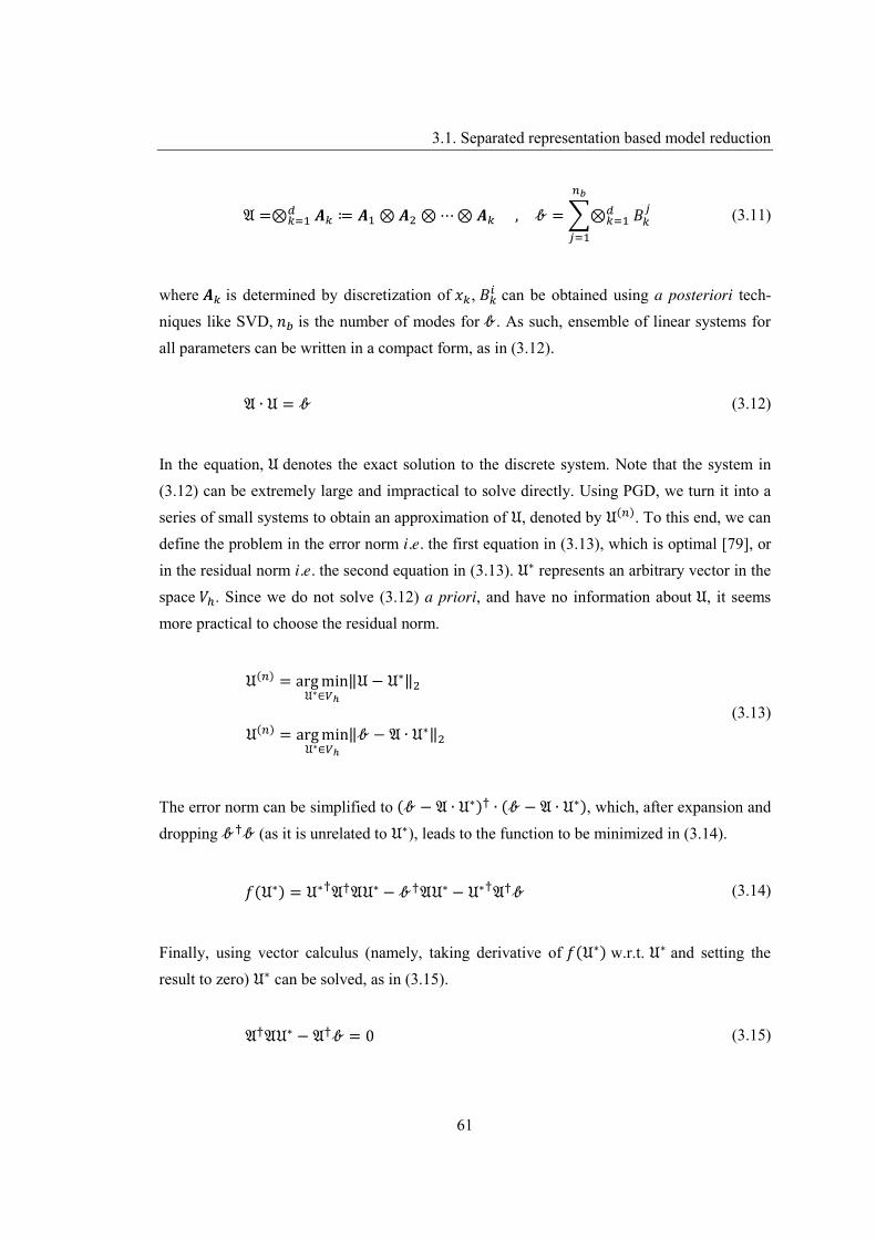
3.1. Separated representation based model reduction
61
𝔄 =⊗ 𝑨 ≔ 𝑨 ⊗ 𝑨 ⊗ ⋯ ⊗ 𝑨 , 𝒷 = ⊗ 𝐵 (3.11)
where 𝑨 is determined by discretization of 𝑥 , 𝐵 can be obtained using a posteriori tech-niques like SVD, 𝑛 is the number of modes for 𝒷. As such, ensemble of linear systems for all parameters can be written in a compact form, as in (3.12).
𝔄 ∙ 𝔘 = 𝒷 (3.12)
In the equation, 𝔘 denotes the exact solution to the discrete system. Note that the system in (3.12) can be extremely large and impractical to solve directly. Using PGD, we turn it into a series of small systems to obtain an approximation of 𝔘, denoted by 𝔘( ). To this end, we can define the problem in the error norm i.e. the first equation in (3.13), which is optimal [79], or in the residual norm i.e. the second equation in (3.13). 𝔘∗ represents an arbitrary vector in the space 𝑉 . Since we do not solve (3.12) a priori, and have no information about 𝔘, it seems more practical to choose the residual norm.
𝔘( ) = arg min𝔘∗∈
‖𝔘 − 𝔘∗‖
𝔘( ) = arg min𝔘∗∈
‖𝒷 − 𝔄 ∙ 𝔘∗‖ (3.13)
The error norm can be simplified to (𝒷 − 𝔄 ∙ 𝔘∗) ∙ (𝒷 − 𝔄 ∙ 𝔘∗), which, after expansion and dropping 𝒷 𝒷 (as it is unrelated to 𝔘∗), leads to the function to be minimized in (3.14).
𝑓(𝔘∗) = 𝔘∗ 𝔄 𝔄𝔘∗ − 𝒷 𝔄𝔘∗ − 𝔘∗ 𝔄 𝒷 (3.14)
Finally, using vector calculus (namely, taking derivative of 𝑓(𝔘∗) w.r.t. 𝔘∗ and setting the result to zero) 𝔘∗ can be solved, as in (3.15).
𝔄 𝔄𝔘∗ − 𝔄 𝒷 = 0 (3.15)
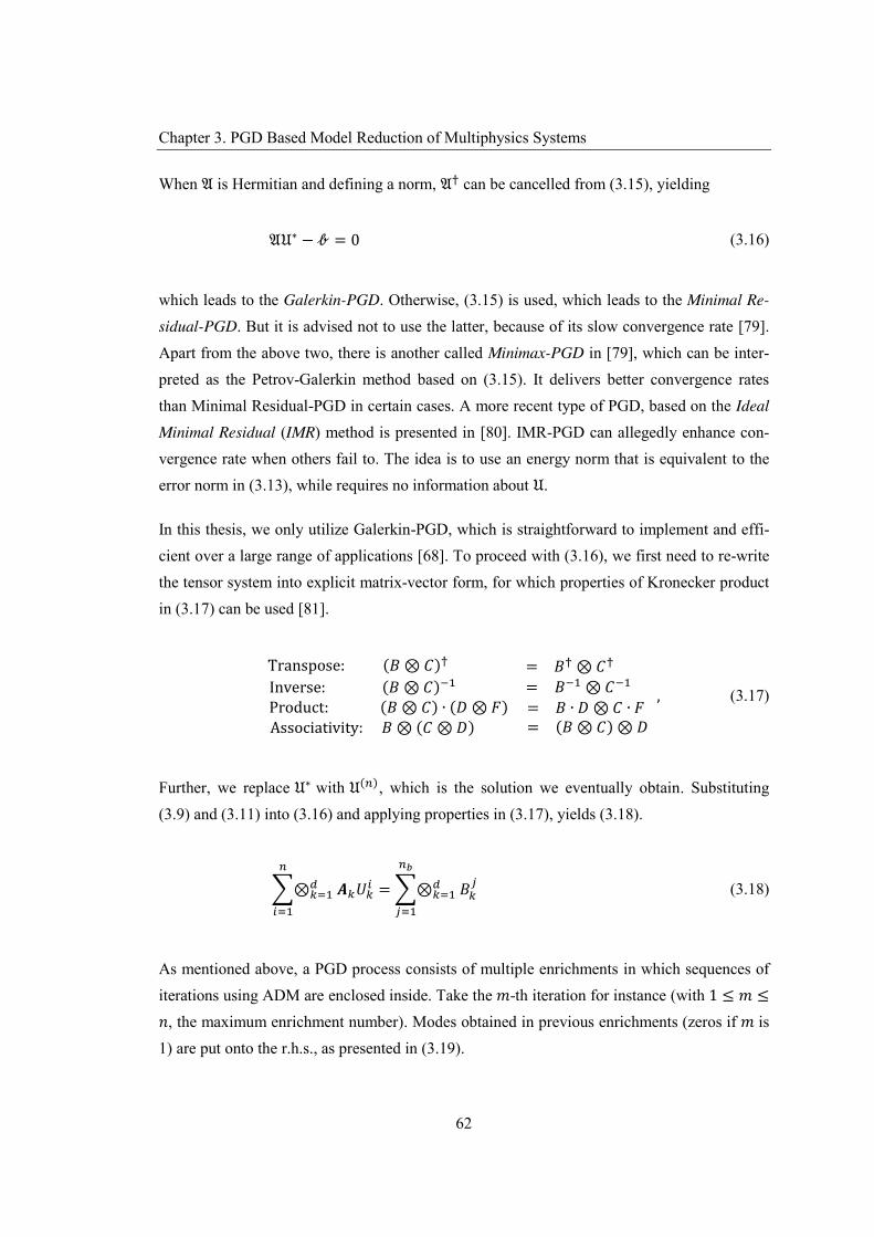
Chapter 3. PGD Based Model Reduction of Multiphysics Systems
62
When 𝔄 is Hermitian and defining a norm, 𝔄 can be cancelled from (3.15), yielding
𝔄𝔘∗ − 𝒷 = 0 (3.16)
which leads to the Galerkin-PGD. Otherwise, (3.15) is used, which leads to the Minimal Re-sidual-PGD. But it is advised not to use the latter, because of its slow convergence rate [79]. Apart from the above two, there is another called Minimax-PGD in [79], which can be inter-preted as the Petrov-Galerkin method based on (3.15). It delivers better convergence rates than Minimal Residual-PGD in certain cases. A more recent type of PGD, based on the Ideal Minimal Residual (IMR) method is presented in [80]. IMR-PGD can allegedly enhance con-vergence rate when others fail to. The idea is to use an energy norm that is equivalent to the error norm in (3.13), while requires no information about 𝔘.
In this thesis, we only utilize Galerkin-PGD, which is straightforward to implement and effi-cient over a large range of applications [68]. To proceed with (3.16), we first need to re-write the tensor system into explicit matrix-vector form, for which properties of Kronecker product in (3.17) can be used [81].
Transpose: (𝐵 ⊗ 𝐶) Inverse: (𝐵 ⊗ 𝐶)
= 𝐵 ⊗ 𝐶 = 𝐵 ⊗ 𝐶
Product: (𝐵 ⊗ 𝐶) ∙ (𝐷 ⊗ 𝐹)Associativity: 𝐵 ⊗ (𝐶 ⊗ 𝐷)
= 𝐵 ∙ 𝐷 ⊗ 𝐶 ∙ 𝐹 = (𝐵 ⊗ 𝐶) ⊗ 𝐷
, (3.17)
Further, we replace 𝔘∗ with 𝔘( ), which is the solution we eventually obtain. Substituting(3.9) and (3.11) into (3.16) and applying properties in (3.17), yields (3.18).
⊗ 𝑨 𝑈 = ⊗ 𝐵 (3.18)
As mentioned above, a PGD process consists of multiple enrichments in which sequences of iterations using ADM are enclosed inside. Take the 𝑚-th iteration for instance (with 1 ≤ 𝑚 ≤𝑛, the maximum enrichment number). Modes obtained in previous enrichments (zeros if 𝑚 is 1) are put onto the r.h.s., as presented in (3.19).
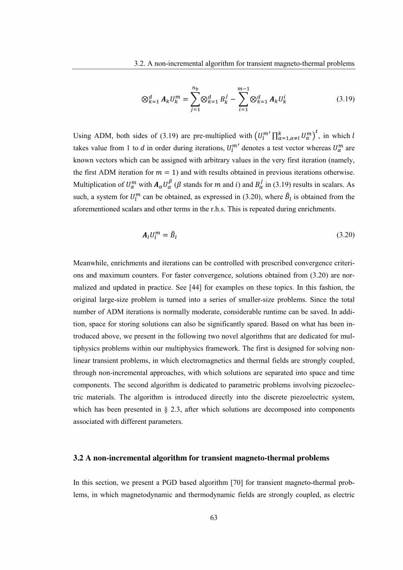
3.2. A non-incremental algorithm for transient magneto-thermal problems
63
⊗ 𝑨 𝑈 = ⊗ 𝐵 − ⊗ 𝑨 𝑈 (3.19)
Using ADM, both sides of (3.19) are pre-multiplied with 𝑈 ∏ 𝑈, , in which 𝑙 takes value from 1 to 𝑑 in order during iterations, 𝑈 denotes a test vector whereas 𝑈 are known vectors which can be assigned with arbitrary values in the very first iteration (namely, the first ADM iteration for 𝑚 = 1) and with results obtained in previous iterations otherwise. Multiplication of 𝑈 with 𝑨 𝑈 (𝛽 stands for 𝑚 and 𝑖) and 𝐵 in (3.19) results in scalars. As such, a system for 𝑈 can be obtained, as expressed in (3.20), where 𝐵 is obtained from the aforementioned scalars and other terms in the r.h.s. This is repeated during enrichments.
𝑨 𝑈 = 𝐵 (3.20)
Meanwhile, enrichments and iterations can be controlled with prescribed convergence criteri-ons and maximum counters. For faster convergence, solutions obtained from (3.20) are nor-malized and updated in practice. See [44] for examples on these topics. In this fashion, the original large-size problem is turned into a series of smaller-size problems. Since the total number of ADM iterations is normally moderate, considerable runtime can be saved. In addi-tion, space for storing solutions can also be significantly spared. Based on what has been in-troduced above, we present in the following two novel algorithms that are dedicated for mul-tiphysics problems within our multiphysics framework. The first is designed for solving non-linear transient problems, in which electromagnetics and thermal fields are strongly coupled, through non-incremental approaches, with which solutions are separated into space and time components. The second algorithm is dedicated to parametric problems involving piezoelec-tric materials. The algorithm is introduced directly into the discrete piezoelectric system, which has been presented in § 2.3, after which solutions are decomposed into components associated with different parameters.
3.2 A non-incremental algorithm for transient magneto-thermal problems
In this section, we present a PGD based algorithm [70] for transient magneto-thermal prob-lems, in which magnetodynamic and thermodynamic fields are strongly coupled, as electric
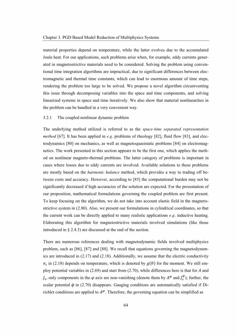
Chapter 3. PGD Based Model Reduction of Multiphysics Systems
64
material properties depend on temperature, while the latter evolves due to the accumulated Joule heat. For our applications, such problems arise when, for example, eddy currents gener-ated in magnetostrictive materials need to be considered. Solving the problem using conven-tional time integration algorithms are impractical, due to significant differences between elec-tromagnetic and thermal time constants, which can lead to enormous amount of time steps, rendering the problem too large to be solved. We propose a novel algorithm circumventing this issue through decomposing variables into the space and time components, and solving linearized systems in space and time iteratively. We also show that material nonlinearities in the problem can be handled in a very convenient way.
3.2.1 The coupled nonlinear dynamic problem
The underlying method utilized is referred to as the space-time separated representation method [67]. It has been applied in e.g. problems of rheology [82], fluid flow [83], and elec-trodynamics [80] on mechanics, as well as magnetoquasistatic problems [84] on electromag-netics. The work presented in this section appears to be the first one, which applies the meth-od on nonlinear magneto-thermal problems. The latter category of problems is important in cases where losses due to eddy currents are involved. Available solutions to these problems are mostly based on the harmonic balance method, which provides a way to trading off be-tween costs and accuracy. However, according to [85] the computational burden may not be significantly decreased if high accuracies of the solution are expected. For the presentation of our proposition, mathematical formulations governing the coupled problem are first present. To keep focusing on the algorithm, we do not take into account elastic field in the magneto-strictive system in (2.80). Also, we present our formulations in cylindrical coordinates, so that the current work can be directly applied to many realistic applications e.g. inductive heating. Elaborating this algorithm for magnetostrictive materials involved simulations (like those introduced in § 2.4.3) are discussed at the end of the section.
There are numerous references dealing with magnetodynamic fields involved multiphysics problem, such as [86], [87] and [88]. We recall that equations governing the magnetodynam-ics are introduced in (2.17) and (2.18). Additionally, we assume that the electric conductivity 𝜎 in (2.18) depends on temperature, which is denoted by 𝑔(𝜃) for the moment. We still em-ploy potential variables in (2.69) and start from (2.70), while differences here is that for 𝐴 and 𝐽 , only components in the 𝜑 axis are non-vanishing (denote them by 𝐴 and 𝐽 ); further, the scalar potential 𝜙 in (2.70) disappears. Gauging conditions are automatically satisfied if Di-richlet conditions are applied to 𝐴 . Therefore, the governing equation can be simplified as
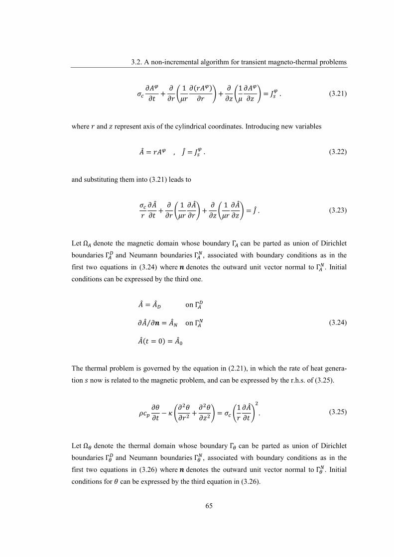
3.2. A non-incremental algorithm for transient magneto-thermal problems
65
𝜎𝜕𝐴𝜕𝑡
+𝜕
𝜕𝑟1
𝜇𝑟𝜕(𝑟𝐴 )
𝜕𝑟+
𝜕𝜕𝑧
1𝜇
𝜕𝐴𝜕𝑧
= 𝐽 . (3.21)
where 𝑟 and 𝑧 represent axis of the cylindrical coordinates. Introducing new variables
𝐴 = 𝑟𝐴 , 𝐽 = 𝐽 . (3.22)
and substituting them into (3.21) leads to
𝜎𝑟
𝜕𝐴𝜕𝑡
+𝜕
𝜕𝑟1
𝜇𝑟𝜕𝐴𝜕𝑟
+𝜕
𝜕𝑧1
𝜇𝑟𝜕𝐴𝜕𝑧
= 𝐽 . (3.23)
Let Ω denote the magnetic domain whose boundary Γ can be parted as union of Dirichletboundaries Γ and Neumann boundaries Γ , associated with boundary conditions as in thefirst two equations in (3.24) where 𝒏 denotes the outward unit vector normal to Γ . Initialconditions can be expressed by the third one.
𝐴 = 𝐴 on Γ
𝜕𝐴 𝜕𝒏⁄ = 𝐴 on Γ
𝐴(𝑡 = 0) = 𝐴
(3.24)
The thermal problem is governed by the equation in (2.21), in which the rate of heat genera-tion 𝑠 now is related to the magnetic problem, and can be expressed by the r.h.s. of (3.25).
𝜌𝑐𝜕𝜃𝜕𝑡
− 𝜅𝜕 𝜃𝜕𝑟
+𝜕 𝜃𝜕𝑧
= 𝜎1𝑟
𝜕𝐴𝜕𝑡
. (3.25)
Let Ω denote the thermal domain whose boundary Γ can be parted as union of Dirichletboundaries Γ and Neumann boundaries Γ , associated with boundary conditions as in thefirst two equations in (3.26) where 𝒏 denotes the outward unit vector normal to Γ . Initialconditions for 𝜃 can be expressed by the third equation in (3.26).

Chapter 3. PGD Based Model Reduction of Multiphysics Systems
66
𝜃 = 𝜃 on Γ
−𝜅 ∙ 𝜕𝜃 𝜕𝒏⁄ = 𝑠 on Γ
𝜃(𝑡 = 0) = 𝜃
(3.26)
3.2.2 Conventional time integration approach
Weak forms of the coupled problem can be obtained by pre-multiplying equations in (3.23) and (3.25) with test functions 𝐴 and 𝜃′, respectively, and integrating the resultant systemover corresponding domains, as expressed in (3.27).
𝐴𝜎𝑟
𝜕𝐴𝜕𝑡
+1
𝜇𝑟𝜕 𝐴𝜕𝑟
+𝜕 𝐴𝜕𝑧
− 𝐽 𝑑Ω = 0
𝜃′ 𝜌𝑐𝜕𝜃𝜕𝑡
− 𝜅𝜕 𝜃𝜕𝑟
+𝜕 𝜃𝜕𝑧
− 𝜎1𝑟
𝜕𝐴𝜕𝑡
𝑑Ω = 0
(3.27)
Next, we treat the problem in (3.27) the same fashion as in Chapter 2; namely, we use the same triangulations for Ω and Ω , then solve magnetic and thermal unknowns simultaneous-ly. Denote the triangulation by Ω , which is the union of 𝑛 FEs. Equations in (3.27) can beprojected onto finite-dimensional spaces. For simplicity, 𝜎 and 𝑟 are approximated as ele-ment-wise constant (denote them as 𝜎 and 𝑟 for the element 𝒦 ), as expressed in (3.28).
𝐴𝜎𝑟
𝜕𝐴𝜕𝑡
+1
𝜇𝑟𝜕 𝐴𝜕𝑟
+𝜕 𝐴𝜕𝑧
− 𝐽 𝑑Ω = 0𝒦
𝜃′ 𝜌𝑐𝜕𝜃𝜕𝑡
− 𝜅𝜕 𝜃𝜕𝑟
+𝜕 𝜃𝜕𝑧
−𝜎𝑟
𝜕𝐴𝜕𝑡𝒦
𝑑Ω = 0
(3.28)
Techniques used for 2D Cartesian coordinate system based FE problems can be directly ap-plied to (3.28). We use 2D nodal elements (defined in (2.16)) for discretization. Over 𝒦 , 𝐴 and 𝜃 are interpolated with shape functions 𝑊 , and nodal values 𝐴 and Θ , as depicted in(3.29) where we use superscript ‘†’ in lieu of ‘𝑡’ to avoid confusions in the subsequent.
3.2. A non-incremental algorithm for transient magneto-thermal problems
67
𝐴 = 𝑊 , , 𝐴 , 𝜃 = 𝑊 , , Θ (3.29)
Note that notation 𝐴 is used for both functions and vectors of discrete values, whose meaning are supposed to be told from the context. Eventually, the global FE system can be deduced by following the same procedure as in § 2.3.2.1, as depicted in (3.30). Definitions of terms in the equation are provided in § B.1.
𝑪 (Θ)
𝜕𝐴𝜕𝑡
+ 𝑲 𝐴 = 𝐽
𝑪𝜕Θ𝜕𝑡
+ 𝑲 Θ = 𝑆 Θ, 𝐴
(3.30)
For time discretization, we use the Crank-Nicholson schema, with which ordinary differential equations (ODE) in (3.30) are solved in a step by step fashion. To account for nonlinearity, both the Picard (also referred to as the fixed point method) and Newton method can be em-ployed. However, for a general nonlinear relation 𝑔(𝜃), the Newton method might not be appropriate, because calculating the Jacobian can be very involved. On the other hand, the Picard method is simpler as it linearizes the system at the current time step by substituting results from the previous time step into the nonlinear terms. Nonetheless, the Picard method may converge slowly or fail to converge, if the time step size is large. To prevent this, we choose sufficiently small time steps. The conventional approach is usually referred to as in-cremental, while our PGD based approach is non-incremental.
3.2.3 Non-incremental space-time separation approach
3.2.3.1 Weak form and space-time discretization
Our non-incremental approach is based on PGD, with which it is assumed that functions 𝐴 and 𝜃 admit separation as in (3.31) where subscripts 𝑋 and 𝑡 implies spatial and temporal association, 𝑟 denotes the maximum number of modes, or rank that depends on the prescribed accuracy and maximum counter of enrichments (as presented in the coming sections).
𝐴( ) ≈ 𝐴 𝐴 , 𝜃( ) ≈ 𝜃 𝜃 (3.31)
Chapter 3. PGD Based Model Reduction of Multiphysics Systems
68
Meanwhile, separation of 𝐽 in (3.23) is trivial, as we introduced in § 3.1.2. We present the separation in (3.32), in which 𝑟 represents the number of modes (corresponding to e.g. the number of stranded inductors in reality), 𝐽 and 𝐽 represents, respectively, the unit current density in coils and the time function of electric currents.
𝐽 ≈ 𝐽 𝐽 (3.32)
On the other hand, terms in (3.31) are calculated a priori, through enrichments. With refer-ence to (3.19), we assume that at the 𝑚-th enrichment, the previous 𝑚 − 1 modes are availa-ble, as depicted in (3.33), where 𝐴 𝐴 and 𝜃 𝜃 are new modes to be calculated.
𝐴( ) = 𝐴( ) + 𝐴 𝐴 ∶= 𝐴 𝐴 + 𝐴 𝐴
𝜃( ) = 𝜃( ) + 𝜃 𝜃 ∶= 𝜃 𝜃 + 𝜃 𝜃
(3.33)
At the same time, nonlinear terms involved in the Joule heat source are handled so that at the 𝑚-th enrichment we have
𝜎 = 𝑔 𝜃( ) ,𝜕𝐴𝜕𝑡
=𝜕𝜕𝑡
𝐴( ) = 𝐴𝜕𝐴𝜕𝑡
. (3.34)
Since each mode has both space and time unknowns components, test functions 𝐴 and 𝜃 in (3.27) now correspond to 𝐴 ′𝐴 + 𝐴 𝐴 ′ and 𝜃 ′𝜃 + 𝜃 𝜃 ′, respectively. To obtain the weak form, integrals are now over the entire space-time domain, which can be denoted by Ω⨂Ι. Ω is the spatial domain, whereas Ι is the temporal domain. The weak form is expressed in (3.35), which needs to be projected onto a finite-dimensional subspace (i.e. discretization).
For Ω, we use the same discretization as the in § 3.2.2. For Ι, we also use FE discretization. More precisely, we denote the discrete time domain by Ι , which consists of 𝑡 , 𝑡 , ⋯, 𝑡 with 𝑡 < 𝑡 < ⋯ < 𝑡 (𝑛 is the total number of time instants).

3.2. A non-incremental algorithm for transient magneto-thermal problems
69
𝐴 ′𝐴 + 𝐴 𝐴 ′
⎩⎪⎪⎨
⎪⎪⎧ 𝑔 𝜃( )
𝑟𝜕 𝐴( ) + 𝐴 𝐴
𝜕𝑡+
1𝜇𝑟
𝜕 𝐴( ) + 𝐴 𝐴𝜕𝑟
+𝜕 𝐴( ) + 𝐴 𝐴
𝜕𝑧
− 𝐽 𝐽⎭⎪⎪⎬
⎪⎪⎫
⨂𝑑𝛺𝑑𝛪 = 0
(𝜃 ′𝜃 + 𝜃 𝜃 ′)⨂
⎩⎪⎪⎨
⎪⎪⎧ 𝜌𝑐
𝜕 𝜃( ) + 𝜃 𝜃𝜕𝑡
−
𝜅𝜕 𝜃( ) + 𝜃 𝜃
𝜕𝑟+
𝜕 𝜃( ) + 𝜃 𝜃𝜕𝑧
−𝑔 𝜃( )
𝑟𝐴
𝜕𝐴𝜕𝑡 ⎭
⎪⎪⎬
⎪⎪⎫
𝑑𝛺𝑑𝛪 = 0
(3.35)
The discrete space-time domain can be denoted by Ω ⨂Ι , and expressed as in (3.36) where ℐ denotes the time element 𝑡 , 𝑡 .
Ω ⨂Ι ≔ 𝒦 ⨂ℐ (3.36)
The discrete weak form is obtained through projecting continuous weak forms in (3.35) onto the discrete space-time domain Ω ⨂Ι . The resultant discrete systems are presented in § B.2. We denote solutions to the discrete system by 𝐴 , , 𝐴 , , Θ , , Θ , (which are associated with continuous variables in (3.33) 𝐴 , 𝐴 , 𝜃 , and 𝜃 , respectively).
Further, we denote vectors containing spatial nodal values in 𝒦 and temporal nodal values in ℐ for 𝐴 (respectively, 𝜃) by 𝐴 and 𝐴 (respectively, Θ and Θ ), and the 1D nodal shape functions for time discretization as 𝑊 , . As such, 𝐴 and 𝜃 over the space-time element𝒦 ⨂ℐ can be interpolated as
𝐴 = 𝑊 , , 𝐴 ⨂ 𝑊 , 𝐴 , 𝜃 = 𝑊 , , Θ ⨂ 𝑊 , Θ (3.37)
Eventually, the FE system used to solve for 𝐴 , , 𝐴 , , Θ , , Θ , can be formed, through replacing variables in the discrete weak form (in § B.2) with the interpolants in (3.37). For

Chapter 3. PGD Based Model Reduction of Multiphysics Systems
70
conciseness, we define coefficient matrices 𝑪 , 𝑲 , 𝑴 , 𝑲 , 𝑪 , 𝑲 , 𝑲 , and 𝑴 , that are shape functions related integrals, as presented in § B.3.
3.2.3.2 Enrichment procedure
Obviously, the obtained global system is nonlinear. As introduced in § 3.1.2, ADM can be employed. It this case, ADM consists in iteratively solving the temporal problem − giving
𝐴 , , Θ , then solving for 𝐴 , , Θ , , and the spatial problem − giving 𝐴 , , Θ ,
then solving for 𝐴 , , Θ , . The temporal problem can be formulated by assigning 𝐴 𝐴 ′
to 𝐴 and 𝜃 𝜃 ′ to 𝜃 in (3.35), whereas the spatial problem can be formulated by assigning𝐴 ′𝐴 to 𝐴 and 𝜃 ′𝜃 to 𝜃 . Algebraic systems for the temporal and spatial problem arepresented in respectively, (3.38) and (3.39). Subscripts 𝐴 and 𝜃 of matrices imply magnetic and thermal problems, whereas superscripts 𝑋 and 𝑡 (not for tensor transpose) imply spatial and temporal problems, respectively. Note that vectors 𝐽 , and 𝐽 , result from discretizationof 𝐽 and 𝐽 in (3.32), whereas 𝑆 , and 𝑆 , result from separating the term related to Jouleheat in (3.35).
𝐴 , , 𝑪 𝐴 , 𝑲 + 𝐴 , , 𝑲 𝐴 , 𝑴 𝐴 ,
= − 𝐴 , , 𝑪 𝐴 , 𝑲 + 𝐴 , , 𝑲 𝐴 , 𝑴 𝐴 , + 𝐴 , , 𝑲 𝐽 , 𝑴 𝐽 ,
Θ , , 𝑪 Θ , 𝑲 + Θ , , 𝑲 Θ , 𝑴 Θ ,
= − Θ , , 𝑪 Θ , 𝑲 + Θ , , 𝑲 Θ , 𝑴 Θ , + Θ , , 𝑲 𝑆 , 𝑴 𝑆 ,
(3.38)
𝐴 , , 𝑲 𝐴 , 𝑪 + 𝐴 , , 𝑴 𝐴 , 𝑲 𝐴 ,
= − 𝐴 , , 𝑲 𝐴 , 𝑪 + 𝐴 , , 𝑴 𝐴 , 𝑲 𝐴 , + 𝐴 , , 𝑴 𝐽 , 𝑲 𝐽 ,
Θ , , 𝑲 Θ , 𝑪 + Θ , , 𝑴 Θ , 𝑲 Θ ,
= − Θ , , 𝑲 Θ , 𝑪 + Θ , , 𝑴 Θ , 𝑲 Θ , + Θ , , 𝑴 𝑆 , 𝑲 𝑆 ,
(3.39)
Meanwhile, for equations in (3.31) it might occur that space values turn to infinitely large,

3.2. A non-incremental algorithm for transient magneto-thermal problems
71
while temporal values to infinitely small (thus leading to numerical overflow). To prevent it, we can normalize 𝐴 , and Θ , by dividing them with their corresponding norms. Also, for efficiency considerations, the maximum iteration counter in ADM (denote it by 𝑛 3) can be set to lower than 10. A tolerance of ~10 can be used as converging criterion (denoted by 𝜀 ), which can be utilized as in (3.40). The symbol 𝑌 refers to both 𝐴 and Θ, which applies to (3.41) and (3.42) in the following, too.
‖𝑌 , − 𝑌 , ‖ ‖𝑌 , ‖⁄ ≤ 𝜀 (3.40)
Once 𝐴 , , 𝐴 , , Θ , , and Θ , are calculated, we can obtain approximations for the real solutions as: 𝐴( ) (i.e. ∑ 𝐴 , ⨂𝐴 , ) and Θ( ) (i.e. ∑ Θ , ⨂Θ , ). To improve conver-gence rates, we can update all time components through solving for 𝐴 , and Θ , from (3.41), in which 𝔄 and 𝒷 denote ensemble of the matrices and r.h.s.s corresponding to all time values, 𝑌 , ′ are test vectors. Spatial values 𝑌 , are not updated, because otherwise it results in a very large system (of size (2𝑚 ∙ 𝑛 ) , as a matter of fact). In contrast, the problem size for updating Y , is (2𝑚 ∙ 𝑛 ) , which is much smaller.
Y , ⨂Y , ′ 𝔄 𝑌 , ⨂Y , = 𝑌 , ⨂Y , 𝒷 (3.41)
The enrichment procedure can be terminated when reaching the maximum counter (denoted by 𝑛 ), or the following criterion is satisfied.
‖𝑌 ‖ ‖𝑌 ‖⁄ = ‖𝑌 , ‖ ‖𝑌 , ‖⁄ ≤ 𝜀 (3.42)
The algorithm is summarized and presented in Figure 3.1. We see that during enrichments, iterations for magnetic and thermal problems are actually “no longer coupled” (namely, un-knowns of the magnetic and thermal problems are solved for separately), which makes it possible to solve these two problems in parallel. With the novel algorithm, complexity of the
3 The subscript ‘In’ and ‘Out’ (that is to appear in the following) can be explained from the fact that ADM itera-tions are inside loops that are enclosed by enrichments, which can be called as outside loops.
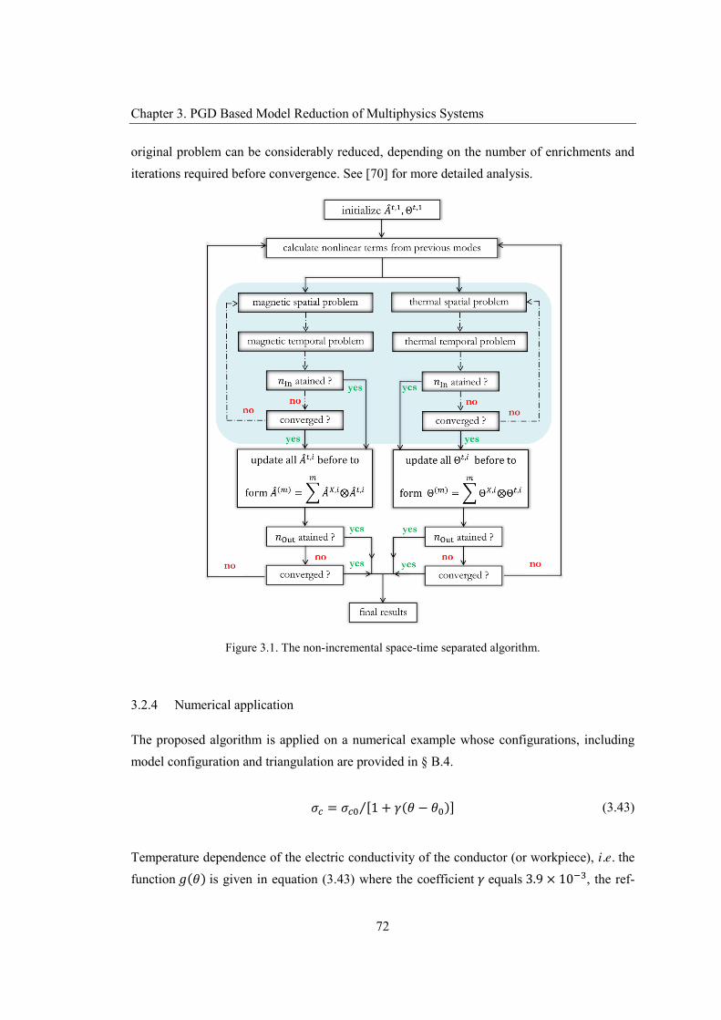
Chapter 3. PGD Based Model Reduction of Multiphysics Systems
72
original problem can be considerably reduced, depending on the number of enrichments and iterations required before convergence. See [70] for more detailed analysis.
Figure 3.1. The non-incremental space-time separated algorithm.
3.2.4 Numerical application
The proposed algorithm is applied on a numerical example whose configurations, including model configuration and triangulation are provided in § B.4.
𝜎 = 𝜎 [1 + 𝛾(𝜃 − 𝜃 )]⁄ (3.43)
Temperature dependence of the electric conductivity of the conductor (or workpiece), i.e. the function 𝑔(𝜃) is given in equation (3.43) where the coefficient 𝛾 equals 3.9 × 10 , the ref-
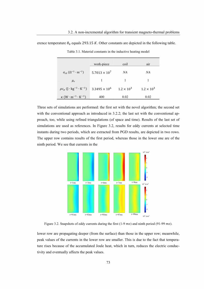
3.2. A non-incremental algorithm for transient magneto-thermal problems
73
erence temperature 𝜃 equals 293.15 𝐾. Other constants are depicted in the following table.
Table 3.1. Material constants in the inductive heating model
work-piece coil air
𝜎 (Ω ∙ m ) 5.7013 × 10⁷ NA NA
𝜇 1 1 1
𝜌𝑐 (J ∙ kg ∙ K ) 3.3495 × 10⁶ 1.2 × 10³ 1.2 × 10³
𝜅 (W ∙ m ∙ K ) 400 0.02 0.02
Three sets of simulations are performed: the first set with the novel algorithm; the second set with the conventional approach as introduced in 3.2.2; the last set with the conventional ap-proach, too, while using refined triangulations (of space and time). Results of the last set of simulations are used as references. In Figure 3.2, results for eddy currents at selected time instants during two periods, which are extracted from PGD results, are depicted in two rows. The upper row contains results of the first period, whereas those in the lower one are of the ninth period. We see that currents in the
Figure 3.2. Snapshots of eddy currents during the first (1-9 𝑚𝑠) and ninth period (91-99 𝑚𝑠).
lower row are propagating deeper (from the surface) than those in the upper row; meanwhile, peak values of the currents in the lower row are smaller. This is due to the fact that tempera-ture rises because of the accumulated Joule heat, which in turn, reduces the electric conduc-tivity and eventually affects the peak values.
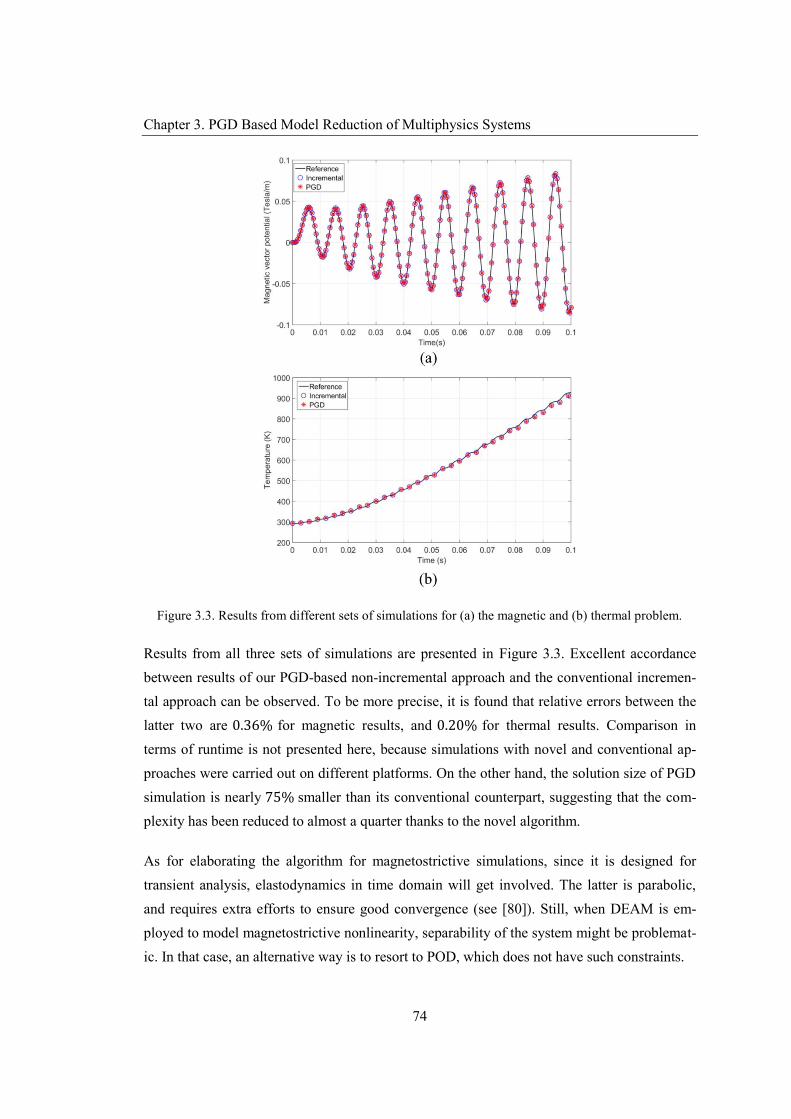
Chapter 3. PGD Based Model Reduction of Multiphysics Systems
74
Figure 3.3. Results from different sets of simulations for (a) the magnetic and (b) thermal problem.
Results from all three sets of simulations are presented in Figure 3.3. Excellent accordance between results of our PGD-based non-incremental approach and the conventional incremen-tal approach can be observed. To be more precise, it is found that relative errors between the latter two are 0.36% for magnetic results, and 0.20% for thermal results. Comparison in terms of runtime is not presented here, because simulations with novel and conventional ap-proaches were carried out on different platforms. On the other hand, the solution size of PGD simulation is nearly 75% smaller than its conventional counterpart, suggesting that the com-plexity has been reduced to almost a quarter thanks to the novel algorithm.
As for elaborating the algorithm for magnetostrictive simulations, since it is designed for transient analysis, elastodynamics in time domain will get involved. The latter is parabolic, and requires extra efforts to ensure good convergence (see [80]). Still, when DEAM is em-ployed to model magnetostrictive nonlinearity, separability of the system might be problemat-ic. In that case, an alternative way is to resort to POD, which does not have such constraints.
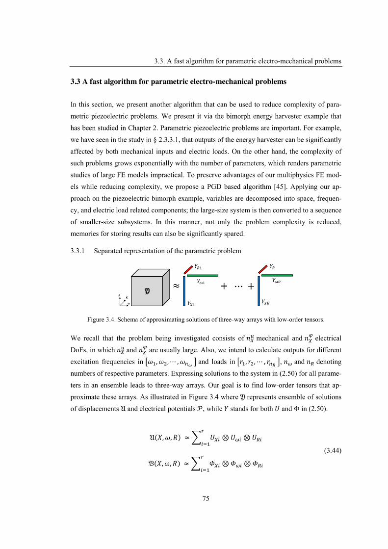
3.3. A fast algorithm for parametric electro-mechanical problems
75
3.3 A fast algorithm for parametric electro-mechanical problems
In this section, we present another algorithm that can be used to reduce complexity of para-metric piezoelectric problems. We present it via the bimorph energy harvester example that has been studied in Chapter 2. Parametric piezoelectric problems are important. For example, we have seen in the study in § 2.3.3.1, that outputs of the energy harvester can be significantly affected by both mechanical inputs and electric loads. On the other hand, the complexity of such problems grows exponentially with the number of parameters, which renders parametric studies of large FE models impractical. To preserve advantages of our multiphysics FE mod-els while reducing complexity, we propose a PGD based algorithm [45]. Applying our ap-proach on the piezoelectric bimorph example, variables are decomposed into space, frequen-cy, and electric load related components; the large-size system is then converted to a sequence of smaller-size subsystems. In this manner, not only the problem complexity is reduced, memories for storing results can also be significantly spared.
3.3.1 Separated representation of the parametric problem
Figure 3.4. Schema of approximating solutions of three-way arrays with low-order tensors.
We recall that the problem being investigated consists of 𝑛 mechanical and 𝑛 electricalDoFs, in which 𝑛 and 𝑛 are usually large. Also, we intend to calculate outputs for differentexcitation frequencies in 𝜔 , 𝜔 , ⋯ , 𝜔 and loads in 𝑟 , 𝑟 , ⋯ , 𝑟 , 𝑛 and 𝑛 denotingnumbers of respective parameters. Expressing solutions to the system in (2.50) for all parame-ters in an ensemble leads to three-way arrays. Our goal is to find low-order tensors that ap-proximate these arrays. As illustrated in Figure 3.4 where 𝔜 represents ensemble of solutions of displacements 𝔘 and electrical potentials 𝒫, while 𝑌 stands for both 𝑈 and Φ in (2.50).
𝔘(𝑋, 𝜔, 𝑅) ≈ 𝑈 ⊗ 𝑈 ⊗ 𝑈
𝔙(𝑋, 𝜔, 𝑅) ≈ 𝛷 ⊗ 𝛷 ⊗ 𝛷
(3.44)
Chapter 3. PGD Based Model Reduction of Multiphysics Systems
76
The approximation can also be expressed by equations in (3.44), where 𝑟 is the rank, while 𝑈 ⊗ 𝑈 ⊗ 𝑈 and 𝛷 ⊗ 𝛷 ⊗ 𝛷 are, respectively, displacement and potential mode.As in (3.11), we also express ensemble of coefficient matrices and r.h.s.s of the system in (2.50) in tensor form. Regarding the r.h.s.s, we assume that identical mechanical excitations are applied in all cases of 𝜔 and 𝑅. Then, the r.h.s. of the whole system can be expressed as 𝐹 ⊗ 𝐹 ⊗ 𝐹 , in which entries of 𝐹 and 𝐹 are all equal to 1, are vectors of size 𝑛 and 𝑛 ,respectively. Regarding coefficient matrices, the expression is straightforward, thanks to our modeling of electric loads and electrodes in § 2.3.2.2, with which variables related to 𝑋, 𝜔 and 𝑅 are individual terms in products. The tensor consists of four blocks, as shown in (3.45).
𝔄 =𝔄 𝔄
𝔄 𝔄 (3.45)
where blocks are defined by
𝔄 ∶= 𝑲 ⊗ 𝑫 ⊗ 𝑫
𝔄 ∶= 𝑲 ⊗ 𝑫 ⊗ 𝑫
𝔄 ∶= 𝑲 ⊗ 𝑫 ⊗ 𝑫 − 𝑗𝑲 ⊗ 𝑮 ⊗ 𝑮
𝔄 ∶= −𝑴 ⊗ 𝑨 ⊗ 𝑫 + 𝑗𝑪 ⊗ 𝑩 ⊗ 𝑫 + 𝑲 ⊗ 𝑫 ⊗ 𝑫
. (3.46)
For definitions in (3.46), 𝑫 and 𝑫 equal identity matrices of respectively 𝑛 and 𝑛 order.Others that are not defined in (2.50) are diagonal matrices, as shown in the following.
𝑨 ≔ diag 𝜔 𝜔 ⋯ 𝜔 ∈ ℝ ×
𝑩 ≔ diag{𝜔 𝜔 ⋯ 𝜔 } ∈ ℝ ×
𝑮 ∶= diag{1 𝑟⁄ 1 𝑟⁄ ⋯ 1 𝑟⁄ } ∈ ℝ ×
𝑮 ∶= diag{1 𝜔⁄ 1 𝜔⁄ ⋯ 1 𝜔⁄ } ∈ ℝ ×
(3.47)
To keep notations neat, we introduce two calligraphic symbols 𝔟 and 𝔵, so that objects can be accessed via subscripts of these latter, see (3.48).
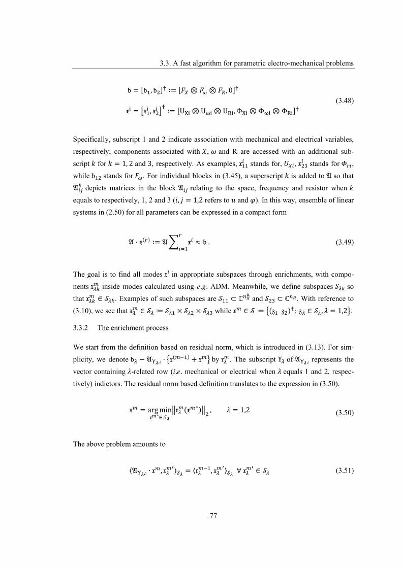
3.3. A fast algorithm for parametric electro-mechanical problems
77
𝔟 = [𝔟 , 𝔟 ] ∶= [𝐹 ⊗ 𝐹 ⊗ 𝐹 , 0]
𝔵 = 𝔵 , 𝔵 ∶= [U ⊗ U ⊗ U , Φ ⊗ Φ ⊗ Φ ](3.48)
Specifically, subscript 1 and 2 indicate association with mechanical and electrical variables, respectively; components associated with 𝑋, 𝜔 and R are accessed with an additional sub-script 𝑘 for 𝑘 = 1, 2 and 3, respectively. As examples, 𝔵 stands for, 𝑈 , 𝔵 stands for 𝛷 , while 𝔟 stands for 𝐹 . For individual blocks in (3.45), a superscript 𝑘 is added to 𝔄 so that 𝔄 depicts matrices in the block 𝔄 relating to the space, frequency and resistor when 𝑘 equals to respectively, 1, 2 and 3 (𝑖, 𝑗 = 1,2 refers to 𝑢 and 𝜑). In this way, ensemble of linear systems in (2.50) for all parameters can be expressed in a compact form
𝔄 ⋅ 𝔵( ) ∶= 𝔄 𝔵 ≈ 𝔟 . (3.49)
The goal is to find all modes 𝔵 in appropriate subspaces through enrichments, with compo-nents 𝔵 inside modes calculated using e.g. ADM. Meanwhile, we define subspaces 𝒮 so that 𝔵 ∈ 𝒮 . Examples of such subspaces are 𝒮 ⊂ ℂ and 𝒮 ⊂ ℂ . With reference to (3.10), we see that 𝔵 ∈ 𝒮 ≔ 𝒮 × 𝒮 × 𝒮 while 𝔵 ∈ 𝒮 ≔ (𝔷 𝔷 ) ; 𝔷 ∈ 𝒮 , 𝜆 = 1,2 .
3.3.2 The enrichment process
We start from the definition based on residual norm, which is introduced in (3.13). For sim-plicity, we denote 𝔟 − 𝔄 ,: ⋅ 𝔵( ) + 𝔵 by 𝔯 . The subscript Υ of 𝔄 ,: represents thevector containing 𝜆-related row (i.e. mechanical or electrical when 𝜆 equals 1 and 2, respec-tively) indictors. The residual norm based definition translates to the expression in (3.50).
𝔵 = arg min𝔵 ∗∈ 𝒮
𝔯 (𝔵 ∗) , 𝜆 = 1,2 (3.50)
The above problem amounts to
⟨𝔄 ,: ∙ 𝔵 , 𝔵 ⟩𝒮 = ⟨𝔯 , 𝔵 ⟩𝒮 ∀ 𝔵 ∈ 𝒮 (3.51)
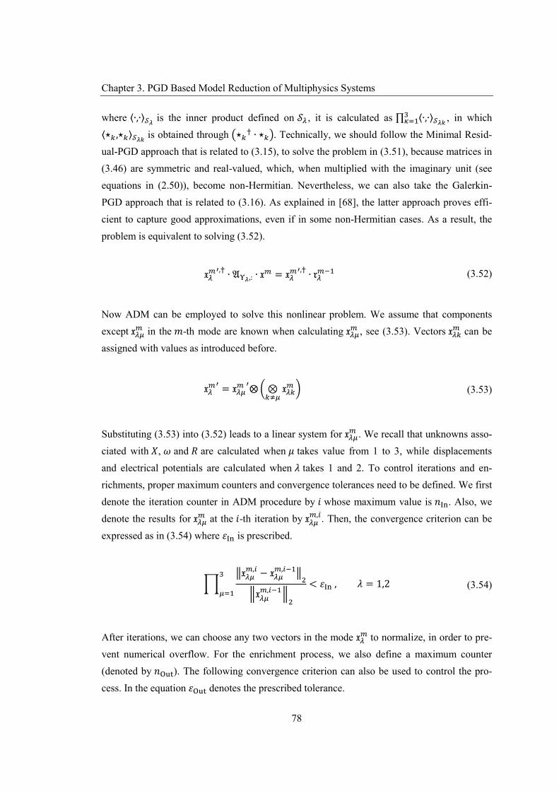
Chapter 3. PGD Based Model Reduction of Multiphysics Systems
78
where ⟨∙,∙⟩𝒮 is the inner product defined on 𝒮 , it is calculated as ∏ ⟨∙,∙⟩𝒮 , in which ⟨⋆ ,⋆ ⟩𝒮 is obtained through ⋆ ∙ ⋆ . Technically, we should follow the Minimal Resid-ual-PGD approach that is related to (3.15), to solve the problem in (3.51), because matrices in (3.46) are symmetric and real-valued, which, when multiplied with the imaginary unit (see equations in (2.50)), become non-Hermitian. Nevertheless, we can also take the Galerkin-PGD approach that is related to (3.16). As explained in [68], the latter approach proves effi-cient to capture good approximations, even if in some non-Hermitian cases. As a result, the problem is equivalent to solving (3.52).
𝔵 , ∙ 𝔄 ,: ∙ 𝔵 = 𝔵 , ∙ 𝔯 (3.52)
Now ADM can be employed to solve this nonlinear problem. We assume that components except 𝔵 in the 𝑚-th mode are known when calculating 𝔵 , see (3.53). Vectors 𝔵 can beassigned with values as introduced before.
𝔵 = 𝔵 ⨂ ⊗ 𝔵 (3.53)
Substituting (3.53) into (3.52) leads to a linear system for 𝔵 . We recall that unknowns asso-ciated with 𝑋, 𝜔 and 𝑅 are calculated when 𝜇 takes value from 1 to 3, while displacements and electrical potentials are calculated when 𝜆 takes 1 and 2. To control iterations and en-richments, proper maximum counters and convergence tolerances need to be defined. We first denote the iteration counter in ADM procedure by 𝑖 whose maximum value is 𝑛 . Also, wedenote the results for 𝔵 at the 𝑖-th iteration by 𝔵 , . Then, the convergence criterion can beexpressed as in (3.54) where 𝜀 is prescribed.
𝔵 , − 𝔵 ,
𝔵 ,< 𝜀 , 𝜆 = 1,2 (3.54)
After iterations, we can choose any two vectors in the mode 𝔵 to normalize, in order to pre-vent numerical overflow. For the enrichment process, we also define a maximum counter (denoted by 𝑛 ). The following convergence criterion can also be used to control the pro-cess. In the equation 𝜀 denotes the prescribed tolerance.
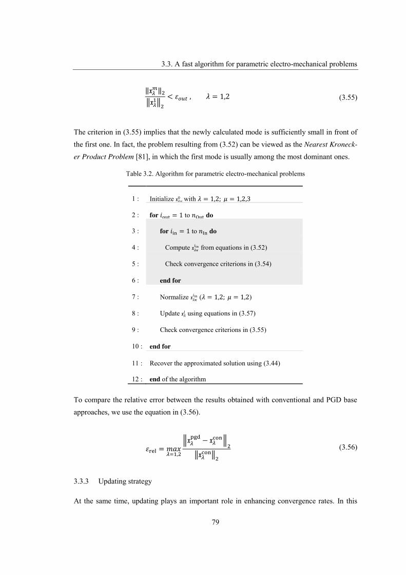
3.3. A fast algorithm for parametric electro-mechanical problems
79
‖𝔵 ‖
𝔵< 𝜀 , 𝜆 = 1,2 (3.55)
The criterion in (3.55) implies that the newly calculated mode is sufficiently small in front of the first one. In fact, the problem resulting from (3.52) can be viewed as the Nearest Kroneck-er Product Problem [81], in which the first mode is usually among the most dominant ones.
Table 3.2. Algorithm for parametric electro-mechanical problems
1 : Initialize 𝔵 with 𝜆 = 1,2; 𝜇 = 1,2,3
2 : for 𝑖 = 1 to 𝑛 do
3 : for 𝑖 = 1 to 𝑛 do
4 : Compute 𝔵 from equations in (3.52)
5 : Check convergence criterions in (3.54)
6 : end for
7 : Normalize 𝔵 (𝜆 = 1,2; 𝜇 = 1,2)
8 : Update 𝔵 using equations in (3.57)
9 : Check convergence criterions in (3.55)
10 : end for
11 : Recover the approximated solution using (3.44)
12 : end of the algorithm
To compare the relative error between the results obtained with conventional and PGD base approaches, we use the equation in (3.56).
𝜀 = 𝑚𝑎𝑥,
𝔵 − 𝔵
𝔵 (3.56)
3.3.3 Updating strategy
At the same time, updating plays an important role in enhancing convergence rates. In this

Chapter 3. PGD Based Model Reduction of Multiphysics Systems
80
case, it can be achieved through enforcing that 𝔯 obtained using the newly calculated mode 𝔵 is orthonormal to the subspace (𝒮 ) ≔ × , , 𝒮 , see (3.57).
𝔵 , ⋅ 𝔟 − 𝔄 ,: ⋅ 𝔵( ) = 0 , 𝑙 = 1,2, … , 𝑚 (3.57)
Again, ADM can be employed to solve (3.57). It consists in solving all 𝑚 components 𝔵while fixing other sets of components 𝔵 for 𝜅 ≠ 𝜇, and take 𝜇 = 1,2,3 in turn. However, itis found in our numerical tests that the convergence rate can be extremely slow, especially when 𝑚 is large. In other words, increasing iteration numbers has insignificant effects in the current case. Consequently, we only perform iteration once in the updating. Also, when up-dating space related components, the problem size is square of 𝑚 × 𝑛 + 𝑛 , which quick-ly goes large as 𝑚 increases. Thus, we do not consider updating space related components. The algorithm is summarized and presented in Table 3.2.
3.3.4 Numerical application
The novel algorithm is applied to solve the bimorph example in § 2.3.3.1. For performance comparison, model configuration, and samples values of parameters are kept identical as with the conventional approach. Recall that the number of frequency samples is 600, while that for resistors is six. In contrast to the example in § 3.2.4, the problem of interest here is solved with conventional and PGD based approach on the same platform, using MATLAB.
Table 3.3. Comparison in performance of different implementations
@ 32 G RAM, 3.5G Hz processor runtime Solutions size Relative error
Conventional (sequetial) 11228 s 1144 Mb reference
Conventional (parallel) 5125 s
PGD (without updating) 3094 s 30.72 Mb 0.178
PGD (with updating) 2483 s 8.01×10⁻⁶
In the first set of tests, convergence criterions for iterations and enrichments are set to be 10 and 10 , respectively. Corresponding maximum counters are set to 10 and 100.Meanwhile, conventional approaches in both sequential and parallel (based on the built-in
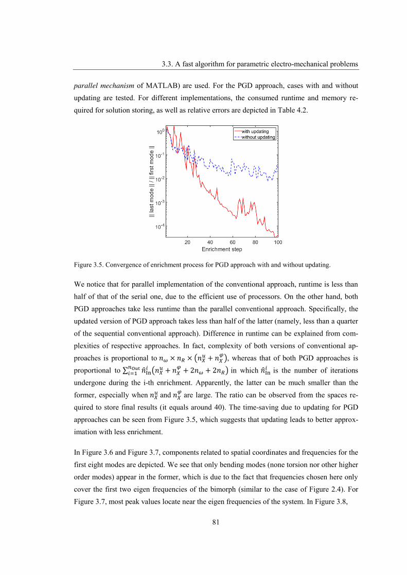
3.3. A fast algorithm for parametric electro-mechanical problems
81
parallel mechanism of MATLAB) are used. For the PGD approach, cases with and without updating are tested. For different implementations, the consumed runtime and memory re-quired for solution storing, as well as relative errors are depicted in Table 4.2.
Figure 3.5. Convergence of enrichment process for PGD approach with and without updating.
We notice that for parallel implementation of the conventional approach, runtime is less than half of that of the serial one, due to the efficient use of processors. On the other hand, both PGD approaches take less runtime than the parallel conventional approach. Specifically, the updated version of PGD approach takes less than half of the latter (namely, less than a quarter of the sequential conventional approach). Difference in runtime can be explained from com-plexities of respective approaches. In fact, complexity of both versions of conventional ap-proaches is proportional to 𝑛 × 𝑛 × 𝑛 + 𝑛 , whereas that of both PGD approaches is proportional to ∑ 𝑛 𝑛 + 𝑛 + 2𝑛 + 2𝑛 in which 𝑛 is the number of iterations undergone during the i-th enrichment. Apparently, the latter can be much smaller than the former, especially when 𝑛 and 𝑛 are large. The ratio can be observed from the spaces re-quired to store final results (it equals around 40). The time-saving due to updating for PGD approaches can be seen from Figure 3.5, which suggests that updating leads to better approx-imation with less enrichment.
In Figure 3.6 and Figure 3.7, components related to spatial coordinates and frequencies for the first eight modes are depicted. We see that only bending modes (none torsion nor other higher order modes) appear in the former, which is due to the fact that frequencies chosen here only cover the first two eigen frequencies of the bimorph (similar to the case of Figure 2.4). For Figure 3.7, most peak values locate near the eigen frequencies of the system. In Figure 3.8,

Chapter 3. PGD Based Model Reduction of Multiphysics Systems
82
Figure 3.6. Components related to spatial coordinates of the first to eighth enrichment. Displacements are depicted by the (scaled) deformation from original positions, while potentials are represented using
the colored region. As in Figure 2.4, area for air is not shown in the figure. Values are normalized.
Figure 3.7. Components related to frequencies of the first to eighth enrichment (Values are normalized).
we depict components related to the resistor of 91 𝑘Ω whose counterparts for other resistors show similar shapes.
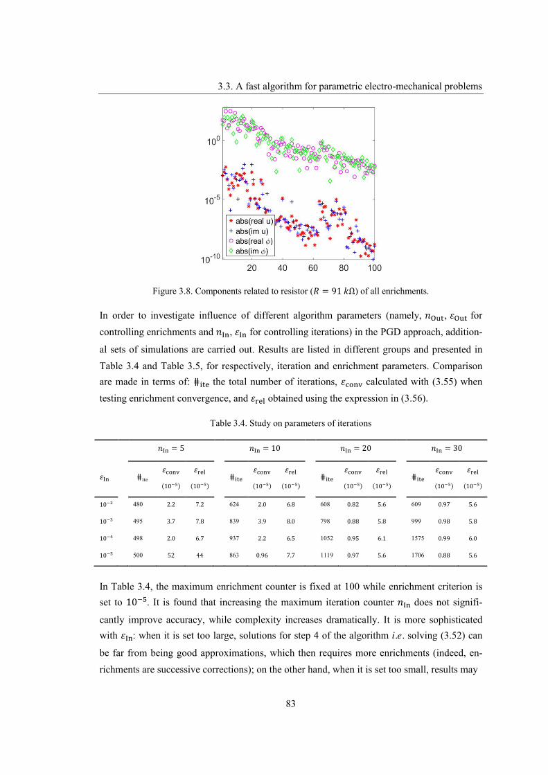
3.3. A fast algorithm for parametric electro-mechanical problems
83
Figure 3.8. Components related to resistor (𝑅 = 91 𝑘Ω) of all enrichments.
In order to investigate influence of different algorithm parameters (namely, 𝑛 , 𝜀 for controlling enrichments and 𝑛 , 𝜀 for controlling iterations) in the PGD approach, addition-
al sets of simulations are carried out. Results are listed in different groups and presented in Table 3.4 and Table 3.5, for respectively, iteration and enrichment parameters. Comparison are made in terms of: ⋕ the total number of iterations, 𝜀 calculated with (3.55) when testing enrichment convergence, and 𝜀 obtained using the expression in (3.56).
Table 3.4. Study on parameters of iterations
𝑛 = 5 𝑛 = 10 𝑛 = 20 𝑛 = 30
𝜀 ⋕𝜀
(10 )
𝜀
(10 ) ⋕
𝜀
(10 )
𝜀
(10 ) ⋕
𝜀
(10 )
𝜀
(10 ) ⋕
𝜀
(10 )
𝜀
(10 )
10 480 2.2 7.2 624 2.0 6.8 608 0.82 5.6 609 0.97 5.6
10 495 3.7 7.8 839 3.9 8.0 798 0.88 5.8 999 0.98 5.8
10 498 2.0 6.7 937 2.2 6.5 1052 0.95 6.1 1575 0.99 6.0
10 500 52 44 863 0.96 7.7 1119 0.97 5.6 1706 0.88 5.6
In Table 3.4, the maximum enrichment counter is fixed at 100 while enrichment criterion is set to 10 . It is found that increasing the maximum iteration counter 𝑛 does not signifi-
cantly improve accuracy, while complexity increases dramatically. It is more sophisticated with 𝜀 : when it is set too large, solutions for step 4 of the algorithm i.e. solving (3.52) can
be far from being good approximations, which then requires more enrichments (indeed, en-richments are successive corrections); on the other hand, when it is set too small, results may

Chapter 3. PGD Based Model Reduction of Multiphysics Systems
84
get deteriorated, because more iterations are needed for higher precision, while it can go di-verging after certain number of iterations. Therefore, the solved modes are not necessarily more accurate, albeit the larger number of iterations.
Table 3.5. Study on parameters of enrichments
𝑛 = 30 𝑛 = 50 𝑛 = 100 𝑛 = 200
𝜀⋕
𝜀
(10 )
𝜀
(10 ) ⋕
𝜀
(10 )
𝜀
(10 ) ⋕
𝜀
(10 )
𝜀
(10 ) ⋕
𝜀
(10 )
𝜀
(10 )
10 228 0.72 4.8 228 7.2 48 228 72 480 228 720 480
10 254 5.7 5.4 417 2.7 1.9 425 8.2 18 425 82 18
10 254 5.7 5.4 417 2.7 1.9 623 0.92 3.6 623 9.2 3.6
10 254 5.7 5.4 417 2.7 1.9 835 0.17 0.69 948 0.82 0.58
In Table 3.5, maximum iteration number is set to 10, iteration convergence criterion is fixed at 10 for all cases. Influences of enrichment parameters are obvious. With more enrich-ment, it is more likely to arrive at better approximations. Thus, both smaller values of 𝜀 and larger values of 𝑛 are in favor of accuracy. However, it is also important to keep in mind
that the limit of approximation precision is also decided by factors other than parame-ters being investigated here, such as updating. Therefore, results are no longer improved to some limit by simply increasing the number of modes. In the present case, maximum counter of 100 and tolerance of 10 are found to be appropriate.
3.4 Chapter summary
In this chapter, we have seen the potential of complexity reducing with separated representa-tions. Based on the latter, POD and PGD are introduced through an abstract problem. We noticed that the former provides good approximations in certain occasions, while subjecting to the number of variables and requiring calculation of the original problem at selected sam-ples of parameter. PGD, on the other hand, can be applied in higher dimensional problems, and construct solutions approximations a priori. Nevertheless, approximations obtained with PGD are normally less optimal than with POD. Besides, effectiveness of the former depends on separability of specific problems.
3.4. Chapter summary
85
Fortunately, the two algorithms that we’ve proposed, based on PGD, prove to be very satis-factory. The first algorithm can be used to significantly reduce problem size of nonlinear magneto-thermal problems. Moreover, when combined with the Picard method, we can solve the strongly-coupled problem in a ‘decoupled’ way, in parallel, thereby, nonlinearity is treated straightforwardly. The second algorithm can be used for large electro-mechanical problems with multiple parameters. In the presented numerical application, our algorithm outperforms the conventional one in terms of runtime and memory requirements, by a large margin, while still delivers highly accurate results (whose relative error is ~10 ).

This page is intentionally left blank.
87
Conclusions and Prospective
In this thesis, a multiphysics finite element framework for piezoelectric and magnetostrictive materials modeling has been presented. We used differential forms based Whitney elements for discretization of quantities of electromagnetic, elastic, and thermal fields. It is shown that the involved fields, as well as coupling effects between these fields, can be conveniently modeled in this framework. Elaborating electrical circuits (including electrodes) into FE sys-tems has also been demonstrated. For constitutive modeling, we adopted the linear piezoelec-tricity for piezoelectric materials, and the free-energy based the discrete energy-averaged model, or DEAM, for magnetostrictive materials. Due to non-homogeneity of magnetostric-tive materials, integration of DEAM with FEM requires that FEM be solved on the macro-scopic structure, and DEAM solved on the microscopic structure. To this end, we have chosen FEs as microscopic representative volumes. As a result, FE results were utilized to extract inputs for DEAM, whereas DEAM results were utilized to assemble FE systems. To deal with nonlinearity involved in this hierarchy, the piecewise linear strategy was adopted. Throughout our numerical tests, we observed that FE models were versatile and able to provide more de-tailed insights into the simulated system than others; however, FE models also demanded more computing resources, especially in cases of transient and parametric analysis. To pre-server advantages of our FE models while reduce the price in terms of runtime and memories; we proposed two novel model reduction algorithms, based on the proper generalized decom-position, or PGD method. In these algorithms, solutions of the multiphysics problem were decomposed into components associated with different parameters, through which the original large-size problem could be converted to a multitude of much smaller-size sub-problems. We presented through a couple of examples that our algorithms were able to significantly reduce problem complexity, while generating very high quality solutions at the same time. To sum up, we have achieved the objectives listed at the beginning of the thesis: 1) building a 3D FE framework to model piezoelectric and magnetostrictive materials involved multiphysics fields and coupling effects; 2) elaborating state-of-the-art constitutive models for better description of materials behaviors; and 3) performing model reduction so as to carry out 3D FE simula-tions efficiently.
In the meanwhile, we also realized that the work presented in this thesis could be extended in some possible orientations. For instance, we noticed that when elastic problems of thin struc-tures involved (for both piezoelectric and magnetostrictive materials), it becomes expensive,
Conclusions and Prospective
88
sometimes problematic to obtain accurate results using our first order elements, due to the well-known shear locking phenomenon. Therefore, it would be helpful to add in higher order elements for such kinds of problems. Also, shell elements can also be considered in such cas-es. Second, although several applications for energy harvesting have been accomplished (and presented) during the thesis, extra efforts are necessary in order to leverage the potential of the developed framework for simulations of devices that are under investigation within our research group. Take the DEAM model for example. Running simulation using the latter re-quires materials specific parameters, which are available for Galfenol and Terfenol-D while currently not for Metglas (per the author’s knowledge). Consequently, additional measure-ments and some fine tuning based on the present work may be needed. Third, for uncertainty quantification it is becoming a trend to perform stochastic simulations for piezoelectric and magnetostrictive materials involved systems, so that a broader range of realistic factors can be accounted for. In this case, our multiphysics models can take the role of modeling the deter-ministic part of the problem, whereas our PGD based algorithms can serve to carry out model reductions in problems related to uncertainties. Last but not the least important, when nonlin-earities in general cases (such as those in DEAM) involved, it becomes questionable for the separability of applying PGD. Therefore, it would be beneficial to investigate novel method-ologies addressing such issue, so that our algorithms can be applied to more general nonlinear problems.
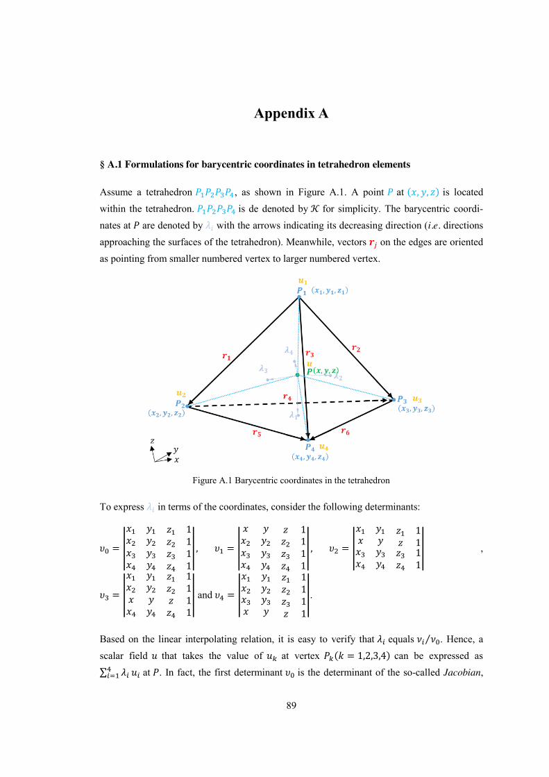
89
Appendix A
§ A.1 Formulations for barycentric coordinates in tetrahedron elements
Assume a tetrahedron 𝑃 𝑃 𝑃 𝑃 , as shown in Figure A.1. A point 𝑃 at (𝑥, 𝑦, 𝑧) is locatedwithin the tetrahedron. 𝑃 𝑃 𝑃 𝑃 is de denoted by 𝒦 for simplicity. The barycentric coordi-nates at 𝑃 are denoted by 𝜆 with the arrows indicating its decreasing direction (i.e. directionsapproaching the surfaces of the tetrahedron). Meanwhile, vectors 𝒓 on the edges are orientedas pointing from smaller numbered vertex to larger numbered vertex.
Figure A.1 Barycentric coordinates in the tetrahedron
To express 𝜆 in terms of the coordinates, consider the following determinants:
𝜐 =
𝑥 𝑦𝑥 𝑦
𝑧 1𝑧 1
𝑥 𝑦𝑥 𝑦
𝑧 1𝑧 1
, 𝜐 =
𝑥 𝑦𝑥 𝑦
𝑧 1𝑧 1
𝑥 𝑦𝑥 𝑦
𝑧 1𝑧 1
, 𝜐 =
𝑥 𝑦𝑥 𝑦
𝑧 1𝑧 1
𝑥 𝑦𝑥 𝑦
𝑧 1𝑧 1
,
𝜐 =
𝑥 𝑦𝑥 𝑦
𝑧 1𝑧 1
𝑥 𝑦𝑥 𝑦
𝑧 1𝑧 1
and 𝜐 =
𝑥 𝑦𝑥 𝑦
𝑧 1𝑧 1
𝑥 𝑦𝑥 𝑦
𝑧 1𝑧 1
.
Based on the linear interpolating relation, it is easy to verify that 𝜆 equals 𝜈 𝜈⁄ . Hence, ascalar field 𝑢 that takes the value of 𝑢 at vertex 𝑃 (𝑘 = 1,2,3,4) can be expressed as∑ 𝜆 𝑢 at 𝑃. In fact, the first determinant 𝜐 is the determinant of the so-called Jacobian,
Appendix
90
denoted by J as in Equation (A.1), which can also be obtained from, e.g. (𝒓 × 𝒓 ) ∙ 𝒓 . The latter is six times of the volume of the tetrahedron (𝜐 = 6|𝒦|).
𝐽 =
𝑥 𝑦𝑥 𝑦
𝑧 1𝑧 1
𝑥 𝑦𝑥 𝑦
𝑧 1𝑧 1
(A.1)
As the barycentric coordinates are first order function, their gradients w.r.t. coordinates 𝑥, 𝑦, and 𝑧 are constant over 𝒦. These constants are shown in Equation (A.2).
grad(𝜆 ) = 𝒓 × 𝒓 6𝜐⁄ , grad(𝜆 ) = 𝒓 × 𝒓 6𝜐⁄grad(𝜆 ) = 𝒓 × 𝒓 6𝜐⁄ , grad(𝜆 ) = 𝒓 × 𝒓 6𝜐⁄ (A.2)
Since all basis function of Whitney elements are calculated via the barycentric coordinates, the above relations allow for a convenient implementation.
§ A.2 Formulations relating the engineering strain and displacement
By definition, the engineering strain tensor 𝜺 within an element 𝒦 is expressed as in Equation (A.3) where (𝑢, 𝑣, 𝑤) represents the displacement of a particle located on the point (𝑥, 𝑦, 𝑧).
𝜺 =
⎣⎢⎢⎢⎢⎡
𝜀 𝜀 𝜀
2𝜀2𝜀2𝜀 ⎦
⎥⎥⎥⎥⎤
=
⎣⎢⎢⎢⎢⎡
𝜕𝑢 𝜕⁄ 𝑥 𝜕𝑣 𝜕⁄ 𝑦
𝜕𝑤 𝜕⁄ 𝑧𝜕𝑢 𝜕⁄ 𝑦 + 𝜕𝑣 𝜕⁄ 𝑥𝜕𝑣 𝜕⁄ 𝑧 + 𝜕𝑤 𝜕⁄ 𝑦𝜕𝑢 𝜕⁄ 𝑧 + 𝜕𝑤 𝜕⁄ 𝑥⎦
⎥⎥⎥⎥⎤
(A.3)
Denote DoFs on 𝒦 – displacements at the 𝑖th vertex for 𝑖 = 1,2,3,4 by (𝑢 , 𝑣 , 𝑤 ), and inter-polate (𝑢, 𝑣, 𝑤) via 𝒶 = ∑ 𝜆 𝒶 for 𝒶 = 𝑢, 𝑣, 𝑤.
Then, insert the interpolants into Euation (A.3) and re-arrange DoFs in a vector as [𝑢 , 𝑣 , 𝑤 , 𝑢 , 𝑣 , 𝑤 , 𝑢 , 𝑣 , 𝑤 , 𝑢 , 𝑣 , 𝑤 ] . As such, 𝜺 can be re-written as

Appendix
91
⎣⎢⎢⎢⎢⎢⎢⎢⎢⎢⎢⎢⎡𝜕𝜆𝜕𝑥
0 0
0𝜕𝜆𝜕𝑦
0
0 0𝜕𝜆𝜕𝑧
𝜕𝜆𝜕𝑥
0 0
0𝜕𝜆𝜕𝑦
0
0 0𝜕𝜆𝜕𝑧
𝜕𝜆𝜕𝑥
0 0
0𝜕𝜆𝜕𝑦
0
0 0𝜕𝜆𝜕𝑧
𝜕𝜆𝜕𝑥
0 0
0𝜕𝜆𝜕𝑦
0
0 0𝜕𝜆
𝜕𝜕𝜆𝜕𝑦
𝜕𝜆𝜕𝑥
0
0𝜕𝜆𝜕𝑧
𝜕𝜆𝜕𝑦
𝜕𝜆𝜕𝑧
0𝜕𝜆𝜕𝑥
𝜕𝜆𝜕𝑦
𝜕𝜆𝜕𝑥
0
0𝜕𝜆𝜕𝑧
𝜕𝜆𝜕𝑦
𝜕𝜆𝜕𝑧
0𝜕𝜆𝜕𝑥
𝜕𝜆𝜕𝑦
𝜕𝜆𝜕𝑥
0
0𝜕𝜆𝜕𝑧
𝜕𝜆𝜕𝑦
𝜕𝜆𝜕𝑧
0𝜕𝜆𝜕𝑥
𝜕𝜆𝜕𝑦
𝜕𝜆𝜕𝑥
0
0𝜕𝜆𝜕𝑧
𝜕𝜆𝜕𝑦
𝜕𝜆𝜕𝑧
0𝜕𝜆𝜕𝑥 ⎦
⎥⎥⎥⎥⎥⎥⎥⎥⎥⎥⎥⎤
⎣⎢⎢⎢⎢⎢⎢⎢⎢⎢⎡𝑢𝑣𝑤𝑢𝑣𝑤𝑢𝑣𝑤𝑢𝑣𝑤 ⎦
⎥⎥⎥⎥⎥⎥⎥⎥⎥⎤
.
Note that nonzero entries in the central large matrix (denoted as 𝑩 ) can be divided into three groups, as marked in different color. Let 𝑩 ,: and 𝑩 :, represent respectively, the ith line and jth colume of 𝑩 . It can be verified that 𝑩 { , , },{ , , , }, 𝑩 { , , },{ , , , }, 𝑩 { , , },{ , , , } all refer to the same matrix :
⎣⎢⎢⎢⎢⎢⎡𝜕𝜆𝜕𝑥
𝜕𝜆𝜕𝑥
𝜕𝜆𝜕𝑦
𝜕𝜆𝜕𝑦
𝜕𝜆𝜕𝑧
𝜕𝜆𝜕𝑧
𝜕𝜆𝜕𝑥
𝜕𝜆𝜕𝑥
𝜕𝜆𝜕𝑦
𝜕𝜆𝜕𝑦
𝜕𝜆𝜕𝑧
𝜕𝜆𝜕𝑧 ⎦
⎥⎥⎥⎥⎥⎤
.
This property of the elastic gradient matrix allows for rapid implementing of the elastic stiff-ness matrix, as the above matrix is very common for FE problems of the scalar field, and can be readily obtained with equation in § A.1. Therefore, while elastic DoFs are vector valued (i.e. three DoFs per vertex) the elastic stiffness matrix can be built based on those of scalar field problems in a straightforward manner.
§ A.3 Calculation of the incident matrices
Denote the number of tetrahedrons, triangles, edges, and nodes in the concerned triangulation by respectively, 𝑛 , 𝑛 , 𝑛 , and 𝑛 . Dimensions of the incident matrices 𝑫, 𝑪, and 𝑮 can thus be expressed as 𝑛 × 𝑛 , 𝑛 × 𝑛 , and 𝑛 × 𝑛 , respectively. Meanwhile, 𝑫, 𝑪, and 𝑮 are composed of values ±1 and 0. Take 𝐶 for example. 𝐶 = 0 means the 𝑗 edge 𝐸 does not locate within the 𝑖 facet 𝐹 . Otherwise, 𝐸 is one of the constituting edges of 𝐹 . Further-more, 𝐶 = +1 implies the local orientation of 𝐸 is consistent with the global orientation, whereas 𝐶 = −1 implies inconsistent.
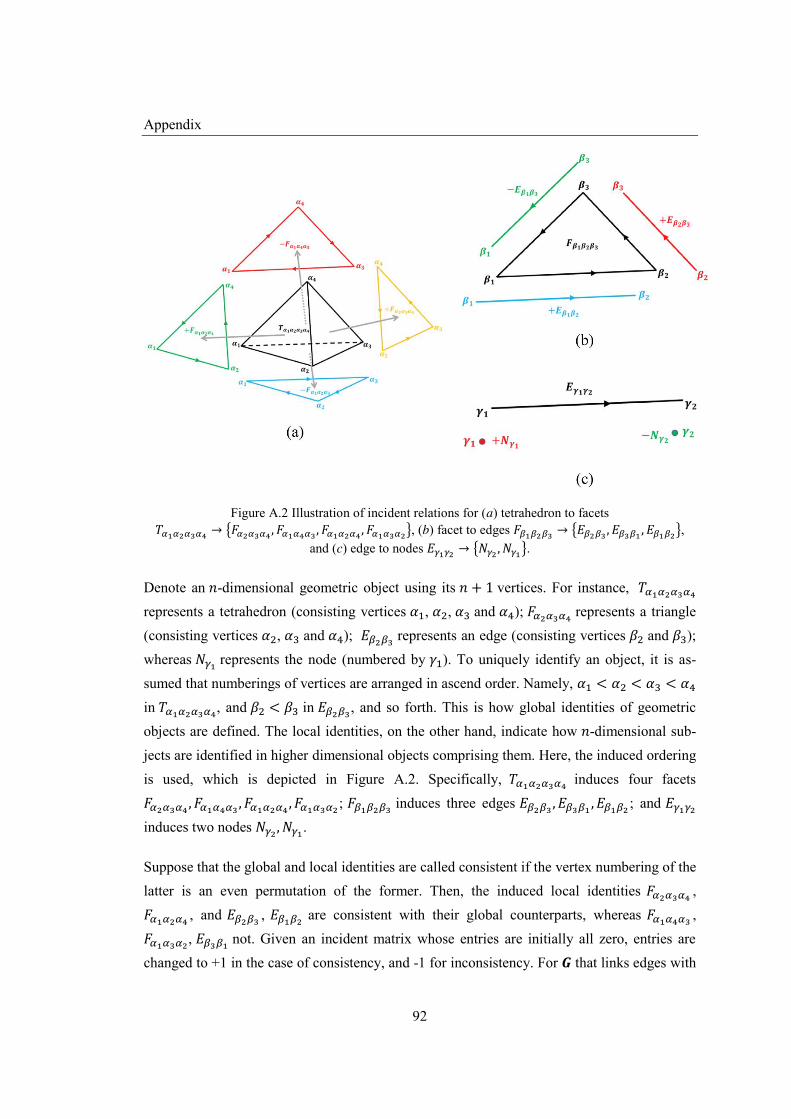
Appendix
92
Figure A.2 Illustration of incident relations for (a) tetrahedron to facets 𝑇 → 𝐹 , 𝐹 , 𝐹 , 𝐹 , (b) facet to edges 𝐹 → 𝐸 , 𝐸 , 𝐸 ,
and (c) edge to nodes 𝐸 → 𝑁 , 𝑁 .
Denote an 𝑛-dimensional geometric object using its 𝑛 + 1 vertices. For instance, 𝑇represents a tetrahedron (consisting vertices 𝛼 , 𝛼 , 𝛼 and 𝛼 ); 𝐹 represents a triangle(consisting vertices 𝛼 , 𝛼 and 𝛼 ); 𝐸 represents an edge (consisting vertices 𝛽 and 𝛽 );whereas 𝑁 represents the node (numbered by 𝛾 ). To uniquely identify an object, it is as-sumed that numberings of vertices are arranged in ascend order. Namely, 𝛼 < 𝛼 < 𝛼 < 𝛼in 𝑇 , and 𝛽 < 𝛽 in 𝐸 , and so forth. This is how global identities of geometricobjects are defined. The local identities, on the other hand, indicate how 𝑛-dimensional sub-jects are identified in higher dimensional objects comprising them. Here, the induced ordering is used, which is depicted in Figure A.2. Specifically, 𝑇 induces four facets𝐹 , 𝐹 , 𝐹 , 𝐹 ; 𝐹 induces three edges 𝐸 , 𝐸 , 𝐸 ; and 𝐸induces two nodes 𝑁 , 𝑁 .
Suppose that the global and local identities are called consistent if the vertex numbering of the latter is an even permutation of the former. Then, the induced local identities 𝐹 ,𝐹 , and 𝐸 , 𝐸 are consistent with their global counterparts, whereas 𝐹 ,𝐹 , 𝐸 not. Given an incident matrix whose entries are initially all zero, entries arechanged to +1 in the case of consistency, and -1 for inconsistency. For 𝑮 that links edges with

Appendix
93
vertices, the second vertex of an edge is assigned with -1, whereas the first with +1. Note that most entries are zero in 𝑫, 𝑪, and 𝑮. As a result, the incident matrices are better stored as sparse matrices,; namely only nonzero entries are stored.
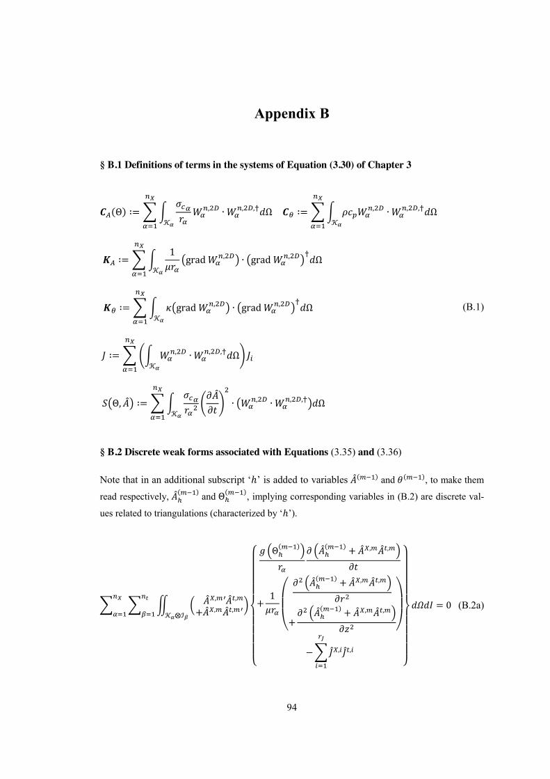
94
Appendix B
§ B.1 Definitions of terms in the systems of Equation (3.30) of Chapter 3
𝑪 (Θ) ∶=𝜎𝑟
𝑊 , ∙ 𝑊 , , 𝑑Ω𝒦
𝑪 ∶= 𝜌𝑐 𝑊 , ∙ 𝑊 , , 𝑑Ω𝒦
𝑲 ∶=1
𝜇𝑟grad 𝑊 , ∙ grad 𝑊 , 𝑑Ω
𝒦
𝑲 ∶= 𝜅 grad 𝑊 , ∙ grad 𝑊 , 𝑑Ω𝒦
𝐽 ∶= 𝑊 , ∙ 𝑊 , , 𝑑Ω𝒦
𝐽
𝑆 Θ, 𝐴 ∶=𝜎𝑟
𝜕𝐴𝜕𝑡
∙ 𝑊 , ∙ 𝑊 , , 𝑑Ω𝒦
(B.1)
§ B.2 Discrete weak forms associated with Equations (3.35) and (3.36)
Note that in an additional subscript ‘ℎ’ is added to variables 𝐴( ) and 𝜃( ), to make them
read respectively, 𝐴( ) and Θ( ), implying corresponding variables in (B.2) are discrete val-
ues related to triangulations (characterized by ‘ℎ’).
𝐴 , ′𝐴 ,
+𝐴 , 𝐴 , ′
⎩⎪⎪⎪⎪⎨
⎪⎪⎪⎪⎧ 𝑔 Θ( )
𝑟𝜕 𝐴( ) + 𝐴 , 𝐴 ,
𝜕𝑡
+1
𝜇𝑟
⎝
⎜⎛
𝜕 𝐴( ) + 𝐴 , 𝐴 ,
𝜕𝑟
+𝜕 𝐴( ) + 𝐴 , 𝐴 ,
𝜕𝑧 ⎠
⎟⎞
− 𝐽 , 𝐽 ,
⎭⎪⎪⎪⎪⎬
⎪⎪⎪⎪⎫
𝒦 ⨂ℐ𝑑𝛺𝑑𝛪 = 0 (B.2a)

Appendix
95
Θ , ′Θ ,
+Θ , Θ , ′
⎩⎪⎪⎪⎪⎨
⎪⎪⎪⎪⎧ 𝜌𝑐
𝜕 Θ( ) + Θ , Θ ,
𝜕𝑡
−𝜅
⎝
⎜⎛
𝜕 Θ( ) + Θ , Θ ,
𝜕𝑟
+𝜕 Θ( ) + Θ , Θ ,
𝜕𝑧 ⎠
⎟⎞
−𝑔 Θ( )
𝑟𝐴 , 𝜕𝐴 ,
𝜕𝑡 ⎭⎪⎪⎪⎪⎬
⎪⎪⎪⎪⎫
𝒦 ⨂ℐ𝑑𝛺𝑑𝛪 = 0 (B.2b)
§ B.3 Coefficient matrices obtained through substituting (3.37) into (B.2)
𝑪 ∶=𝜎𝑟
𝑊 , ∙ 𝑊 , ,
𝒦𝑑𝛺
𝑛𝑋
𝛼=1
𝑲 ∶=1
𝜇𝑟grad 𝑊 , ∙ grad 𝑊 ,
𝒦𝑑𝛺
𝑛𝑋
𝛼=1
𝑪 ∶= 𝜌𝑐 𝑊 , ∙ 𝑊 , ,
𝒦𝑑𝛺
𝑛𝑋
𝛼=1
𝑲 ∶= 𝜅 grad 𝑊 , ∙ grad 𝑊 ,
𝒦𝑑𝛺
𝑛𝑋
𝛼=1
𝑴 ∶= 𝑊 , ∙ 𝑊 , ,
ℐ𝛽
𝑑𝛪𝑛𝑡
𝛽=1𝑲 ∶= 𝑊 , ∙
𝜕𝑊 ,
𝜕𝑡ℐ𝛽
𝑑𝛪𝑛𝑡
𝛽=1
𝑴 ∶= 𝑊 , ∙ 𝑊 , ,
ℐ𝛽
𝑑𝛪𝑛𝑡
𝛽=1𝑲 ∶= 𝑊 , ∙
𝜕𝑊 ,
𝜕𝑡ℐ𝛽
𝑑𝛪𝑛𝑡
𝛽=1
(B.3)
It is worth noting that due to the consistency of time discretization, time basis functions in 𝑲 and 𝑲 are changed from 𝑊 , to 𝑊 , , which equals 𝑊 , + 0.5 ℐ𝛽 ∙ 𝜕𝑊 , 𝜕𝑡⁄ (i.e. the so-called upwind Petrov-Galerkin formulation). ℐ𝛽 is the length of time element ℐ .
§ B.4 Settings for the numerical model in §3.2.4 (inductive heating)
The model consists of a conductor that is axisymmetric to the 𝑧-axis, an excitation coil, and

Appendix
96
an air boxed (of 0.2 𝑚 × 0.5 𝑚). Geometric dimensions related to the conductor and coil are depicted in Figure B.1.a. Linear triangular elements are used to discretize the space domain. Size of elements near the conductor skin is set to be relatively small, so as to account for the skin effect. A total of 5659 elements with 2900 nodes are generated.
Figure B.1 Model configuration (a) geometric dimensions, and (b) spatial triangulation
97
Bibliography
[1] F. K. Shaikh and S. Zeadally, “Energy harvesting in wireless sensor networks: A comprehensive review,” Renew. Sustain. Energy Rev., vol. 55, pp. 1041–1054, 2016.
[2] Z. Deng, “Nonlinear Modeling and Characterization of the Villari Effect and Model-guided Development of Magnetostrictive Energy Harvesters and Dampers,” Ph.D. dissertation, Dept. Mech. Eng., Ohio State Univ., Columbus, OH, US, 2015.
[3] G. Srinivasan, S. Priya, and N. X. Sun, Composite Magnetoelectrics: Materials, Structures and Applications. Woodhead Publishing, Cambridge, UK, 2015.
[4] Y. K. Tan, Energy harvesting autonomous sensor systems, sesign, analysis, and practical implementation. CRC Press, Taylor & Francis Group, Boca Raton, FL, US, 2013.
[5] S. P. Beeby, R. N. Torah, M. J. Tudor, P. Glynne-Jones, T. O’Donnell, C. R. Saha, and S. Roy, “A micro electromagnetic generator for vibration energy harvesting,” J. Micromechanics Microengineering, vol. 17, no. 7, pp. 1257–1265, 2007.
[6] C. Zhao, Ultrasonic Motors. Springer Berlin heidelberg, Germany, 2011.
[7] K. Uchino, Ferroelectric Devices. Marcel Dekker, Inc., New York, NY, US, 2000.
[8] D. Jiles, Introduction to Magnetism and Magnetic Materials. Chapman & Hall, London, UK, 1991.
[9] A. Belahcen, “Magnetoelasticity, Magnetic Forces and Magnetostriction in Electrical Machines,” Ph.D. dissertation, Dept.Elec. Eng., Helsinki University of Technology, Espoo, Finland, 2001.
[10] R. C. Smith, “Smart Material Systems: Model Development.pdf.” SIAM, Philadelphia, US, 2005.
[11] A. Clark and K. Hathaway, “Physics of Giant Magnetostriction,” in Handbook of Giant Magnetostrictive Materials, Academic Press, San Diego, US, 2000.
[12] S. Roundy and P. K. Wright, “A piezoelectric vibration based generator for wireless electronics,” Smart Mater. Struct., vol. 13, no. 5, pp. 1131–1142, 2004.
[13] A. Erturk and D. J. Inman, Piezoelectric Energy Harvesting. John Wiley & Sons, Ltd., West Sussex, UK, 2011.
[14] H. A. Sodano, G. Park, and D. J. Inman, “Estimation of electric charge output for piezoelectric energy harvesting,” Strain, vol. 40, no. 2, pp. 49–58, 2004.
[15] J. Atulasimha and A. B. Flatau, “A review of magnetostrictive iron–gallium alloys,” Smart Mater. Struct., vol. 20, no. 4, p. 43001, 2011.
Bibliography
98
[16] J. Atulasimha, “Characterization and modeling of the magnetomechanical behavior of Iron-Gallium alloys,” Ph.D. dissertation, Dept. Aero. Eng., University of Maryland, College Park, MD, US, 2006.
[17] P. G. Evans and M. J. Dapino, “Efficient magnetic hysteresis model for field and stress application in magnetostrictive Galfenol,” J. Appl. Phys., vol. 107, no. 6, pp. 1–11, 2010.
[18] S. Chakrabarti, “Modeling of 3D Magnetostrictive Systems with Application to Galfenol and Terfenol-D Transducers,” Ph.D. dissertation, Dept. Mech. Eng., Ohio State Univ., Columbus, OH, US, 2011.
[19] J. J. Scheidler, “Static and Dynamic Delta E Effect in Magnetostrictive Materials with Application to Electrically-Tunable Vibration Control Devices,” Ph.D. dissertation, Dept. Mech. Eng., Ohio State Univ., Columbus, OH, US, 2015.
[20] “COMSOL Multiphysics.” [Online]. Available: www.comsol.com.
[21] M. Schinnerl, M. Kaltenbacher, U. Langer, R. Lerch, and J. Schöberl, “An efficient method for the numerical simulation of magneto-mechanical sensors and actuators,” Eur. J. Appl. Math., vol. 18, no. 2, p. 233, 2007.
[22] P. G. Evans and M. J. Dapino, “Dynamic model for 3-D magnetostrictive transducers,” IEEE Trans. Magn., vol. 47, no. 1 PART 2, pp. 221–230, 2011.
[23] J.-M. Jin, The Finite Element Method in Electromagnetics, 3rd edition. John wiley & Sons, Inc., Hoboken, New Jersey, 2014.
[24] O. Bíró, “Edge element formulations of eddy current problems,” Comput. Methods Appl. Mech. Eng., vol. 169, no. 3–4, pp. 391–405, 1999.
[25] T. T. Nguyen, F. Bouillault, L. Daniel, and X. Mininger, “Finite element modeling of magnetic field sensors based on nonlinear magnetoelectric effect,” J. Appl. Phys., vol. 109, no. 8, p. 84904, 2011.
[26] H. Talleb and Z. Ren, “Finite element modeling of magnetoelectric laminate composites in considering nonlinear and load effects for energy harvesting,” J. Alloys Compd., vol. 615, pp. 65–74, 2014.
[27] H. Talleb, A. Gensbittel, and Z. Ren, “Multiphysics modeling of a magnetoelectric composite Rosen-type device,” Compos. Struct., vol. 137, pp. 1–8, 2016.
[28] J. M. Koning, “An Object Oriented , Finite Element Framework For Linear Wave Equations,” PhD dissertation, Univ. of California at Davis, Livermore, CA, US, 2004.
[29] A. Bossavit, Computational Electromagnetism, Variational Formulations, Complementarity, Edge Elements. Academic Press Ltd., London, UK, 1998.
[30] M. Desbrun, E. Kanso, and Y. Tong, “Discrete differential forms for computational modeling,” ACM SIGGRAPH 2006 Courses SIGGRAPH 06, vol. 38, p. 39, 2006.

Bibliography
99
[31] A. N. Hirani, “Discrete Exterior Calculus,” PhD dissertation, California Institute of Technology, Pasadena, CA, US, 2003.
[32] A. Journeaux, “Modélisation multi-physique en génie électrique. Application au couplage magnéto-thermo-mécanique,” PhD dissertation, GeePs, Université Paris Sud - Paris XI, Gif sur Yvette, France, 2013.
[33] J. C. Nedelec, “Mixed finite elements in ℝ3,” Numer. Math., vol. 35, no. 3, pp. 315–341, 1980.
[34] F. L. Teixeira and W. C. Chew, “Lattice electromagnetic theory from a topological viewpoint,” J. Math. Phys., vol. 40, no. 1, pp. 169–187, 1999.
[35] A. Angoshtari and A. Yavari, “A geometric structure-preserving discretization scheme for incompressible linearized elasticity,” Comput. Methods Appl. Mech. Eng., vol. 259, pp. 130–153, 2013.
[36] A. S. Sinwel, “A New Family of Mixed Finite Elements for Elasticity,” PhD dissertation, Institute fuer Numerische Mathematik, Johannes Kepler Univ., Linz, Austria, 2009.
[37] A. . Fallis, P. Freschi, M. Repetto, and C. Rosso, The Cell Method for ElectricalEngineering and Multiphysics Problems - An Introduction. Lecture Notes in Electrical Engineering, Springer, Berlin, Germany, 2013.
[38] I. Doghri, Mechanics of Deformable Solids: Linear, Nonlinear, Analytical andComputational Aspects. Springer-Verlag Berlin Heidelberg, Germany, 2000.
[39] IEEE Standards Board, IEEE Standard on Piezoelectricity. The Institute of Electrical and Electronics Engineers, Inc., New York, NY, US, 1988.
[40] D. Dissanayake (editor), “Acoustic Waves, Chapter 9: Surface acoustic wave based wireless MEMS actuators for biomedical applications,” Sciyo, Rijeka, Croatia, 2010.
[41] J. L. Coulomb, F. X. Zgainski, and Y. Maréchal, “A pyramidal element to link hexahedral, prismatic and tetrahedral edge finite elements,” IEEE Trans. Magn., vol. 33, no. 2, pp. 1362–1365, 1997.
[42] S. Zhao and a Erturk, “Electroelastic modeling and experimental validations of piezoelectric energy harvesting from broadband random vibrations of cantilevered bimorphs,” Smart Mater. Struct., vol. 22, no. 1, p. 15002, 2013.
[43] J. S. Wang and D. F. Ostergaard, “Finite element-electric circuit coupled simulation method,” IEEE Ultrason. Symp., pp. 1105–1108, 1999.
[44] Z. Qin, H. Talleb, J. Y. Duquesne, M. Marangolo, and Z. Ren, “Finite-element modeling of thermoelastic attenuation in piezoelectric surface acoustic wave devices,” IEEE Trans. Magn., vol. 51, no. 3, pp. 2–5, 2015.
[45] Z. Qin, H. Talleb, S. Yan, X. Xu, and Z. Ren, “Application of PGD on parametric

Bibliography
100
modeling of a piezoelectric energy harvester,” IEEE Trans. Magn., vol. 52, no. 11 pp. 7210211, 2016.
[46] F. Wein, “Topology optimization of smart piezoelectric transducers,” PhD dissertation, Engineering Faculty, Univ. Erlangen-Nuernberg, Nuernberg, Germany, 2011.
[47] A.P. Mayer, “Thermoelastic attenuation of surface acoustic waves in elastic media,” J.Appl. Phys, vol. 68, no. 11, pp. 5913–5915, 1990.
[48] G. Engdahl, “Modeling of giant magnetostrictive materials,” in Handbook of GiantMagnetostrictive Materials, Academic Press, San Diego, US, 2000.
[49] IEEE Standards Board, “IEEE Standard on Magnetostrictive Materials: Piezomagnetic Nomenclature,” IEEE Trans. Sonics Ultrason., vol. 20, pp. 67–77, 1973.
[50] H. Tari, J. J. Scheidler, and M. J. Dapino, “Robust solution procedure for the discrete energy-averaged model on the calculation of 3D hysteretic magnetization and magnetostriction of iron–gallium alloys,” J. Magn. Magn. Mater., vol. 384, pp. 266–275, 2015.
[51] S. Clénet, “Model with source terms in the constitutive relationship,” IEEE Trans.Magn., vol. 38, no. 2 I, pp. 481–484, 2002.
[52] T. Henneron, S. Clénet, P. Dular, and F. Piriou, “Discrete finite element characterizations of source fields for volume and boundary constraints in electromagnetic problems,” J. Comput. Appl. Math., vol. 215, no. 2, pp. 438–447, 2008.
[53] J. F. Blackburn, M. Vopsaroiu, and M. G. Cain, “Verified finite element simulation of multiferroic structures: Solutions for conducting and insulating systems,” J. Appl.Phys., vol. 104, no. 7, pp. 1–14, 2008.
[54] I. Oezdemir, W. A. M. Brekelmans, and G. M.G.D., “Computational homogenization for heat conduction in heterogeneous solids,” Int. J. Numer. Meth. Engng, vol. 73, pp. 185–204, 2008.
[55] S. Chakrabarti and M. J. Dapino, “Nonlinear finite element model for 3D Galfenol systems,” Smart Mater. Struct., vol. 20, no. 10, p. 105034, 2011.
[56] A. C. Antoulas, D. . Sorensen, and S. Gugercin, “A survey of model reduction methods for large-scale systems,” Comtenporary Math., vol. 280, pp. 193–219, 2001.
[57] T. Croft, “Proper Generalised Decompositions: theory and applications,” PhD dissertation, School of Mathematics, Cardiff Univ., Cardiff, Wales, UK, 2015.
[58] Y. C. Liang, H. P. Lee, S. P. Lim, W. Z. Lin, K. H. Lee, and C. G. Wu, “Proper Orthogonal Decomposition and its applications—Part I: Theory,” J. Sound Vib., vol. 252, no. 3, pp. 527–544, 2002.
Bibliography
101
[59] A. Ammar, B. Mokdad, F. Chinesta, and R. Keunings, “A new family of solvers for some classes of multidimensional partial differential equations encountered in kinetic theory modeling of complex fluids,” J. Nonnewton. Fluid Mech., vol. 139, no. 3, pp. 153–176, 2006.
[60] U. Baur, P. Benner, and L. Feng, “Model Order Reduction for Linear and Nonlinear Systems: A System-Theoretic Perspective,” Arch. Comput. Methods Eng., vol. 21, no. 4, pp. 331–358, 2014.
[61] S. Chaturantabut and D. C. Sorensen, “Nonlinear model reduction via discrete empirical interpolation,” SIAM J. Sci. Comput., vol. 32, no. 5, pp. 2737–2764, 2010.
[62] A. M. Lattimer, “Model Reduction of Nonlinear Fire Dynamics Models,” PhD dissertation, Dept. of Mathematics, Virginia Polytechnic Institute and State Univ., Blacksburg VI, US, 2016.
[63] G. Rozza, D. B. P. Huynh, and A. T. Patera, “Reduced basis approximation and a posteriori error estimation for affinely parametrized elliptic coercive partial differential equations: Application to transport and continuum mechanics,” Arch. Comput.Methods Eng., vol. 15, no. 3, pp. 229–275, 2008.
[64] M. Capaldo, “A new approximation framework for PGD-based nonlinear solvers,” PhD dissertation, Ecole doctorale SMEMG, Univ. Paris-Saclay, Cachan, France, 2015.
[65] T. Henneron and S. Clénet, “Model order reduction of nonlinear magnetostatic problems based on POD and DEI methods,” IEEE Trans. Magn., vol. 50, no. 2, p. 7000604, 2014.
[66] T. Henneron and S. Clénet, “Model-order reduction of multiple-input non-linear systems based on POD and DEI methods,” IEEE Trans. Magn., vol. 51, no. 3, pp. 7207104, 2015.
[67] A. Ammar, B. Mokdad, F. Chinesta, and R. Keunings, “A new family of solvers for some classes of multidimensional partial differential equations encountered in kinetic theory modelling of complex fluids. Part II: Transient simulation using space-time separated representations,” J. Nonnewton. Fluid Mech., vol. 144, no. 2–3, pp. 98–121, 2007.
[68] M. Chevreuil and A. Nouy, “A model order reduction based on proper generalized decomposition for the propagation of uncertainty in structural dynamics,” Int. J.Numer. Meth. Engng, vol. 89, no. 2, pp. 241–268, 2012.
[69] P. Ladevèze, Nonlinear Computational Structural Mechanics: New Approaches andNon-Incremental Methods of Calculation. Springer Verlag, New York, NY, US, 1999.
[70] Z. Qin, H. Talleb, and Z. Ren, “A proper generalized decomposition-based solver for nonlinear magnetothermal problems,” IEEE Trans. Magn., vol. 52, no. 2, p. 7400209, 2016.
[71] T. Henneron and S. Clénet, “Application of the PGD and DEI methods to solve a

Bibliography
102
nonlinear magnetostatic problem coupled with the circuit equations,” IEEE Trans. Magn., vol. 52, no. 3, p. 7202104, 2016.
[72] A. Nouy, “Low-rank tensor methods for model order reduction,” arXiv: 1511.01554 [math.NA], 2015.
[73] L. Grasedyck, D. Kressner, and C. Tobler, “A literature survey of low-rank tensor approximation techniques,” Gesellschaft fuer Angew. Math. und Mech. - Mitteilungen, vol. 36, no. 1, pp. 53–78, 2013.
[74] E. Pruliere, F. Chinesta, and A. Ammar, “On the deterministic solution of multidimensional parametric models using the proper generalized decomposition,” Math. Comput. Simulat., vol. 81, no. 4, pp. 791–810, 2010.
[75] S. Nirromandi, D. Gonzales, I. Alfaro, and E. Al, “Real-time simulation of biological soft tissues: a PGD approach,” Int. J. Numer. Meth. Engng, vol. 29, no. 5, pp. 586–600, 2013.
[76] D. Yang, Z. M. Ma, and A. Buja, “A sparse SVD method for high-dimensional data,” arXiv: 1112.2433v1 [stat.ME], 2011.
[77] J. V Aguado, “Advanced strategies for the separated formulation of problems in the Proper Generalized Decomposition framework,” PhD dissertation, Ecole doctorale SPIGA, Univ. Nantes Anger Le Mans, Nante, France, 2015.
[78] D. Modesto, S. Zlotnik, and A. Huerta, “Proper generalized decomposition for parameterized Helmholtz problems in heterogeneous and unbounded domains,” Comput. Methods Appl. Mech. Eng., vol. 295, no. 1, pp. 127–149, 2015.
[79] A. Nouy, “A priori model reduction through proper generalized decomposition for solving time-dependent partial differential equations,” Comput. Methods Appl. Mech. Eng., vol. 199, no. 23, pp. 1603–1626, 2010.
[80] L. Boucinha, A. Ammar, A. Gravouil, and A. Nouy, “Ideal minimal residual-based proper generalized decomposition for non-symmetric multi-field models - Application to transient elastodynamics in space-time domain,” Comput. Methods Appl. Mech. Eng., vol. 273, pp. 56–76, 2014.
[81] G. H. Golub and C. F. Van Loan, Matrix Computations, 4th Edition. The Johns Hopkins University Press, Baltimore, MD, US, 2013.
[82] A. Ammar, M. Normandin, F. Daim, D. Gonzale, E. Cueto, and F. Chinesta, “Non incremental strategies based on separated representaions: application in computational rheology,” Commun. Math. Sci., vol. 8, no. 3, pp. 671–695, 2010.
[83] A. Dumon, C. Allery, and A. Ammar, “Proper generalized decomposition for the resolution of Navier-Stokes equations,” J. Comput. Phys., vol. 230, no. 4, pp. 1387–1407, 2011.
[84] T. Henneron and S. Clénet, “Proper generalized decomposition method applied to
Bibliography
103
solve 3D magnetoquasi-static field problems coupling with external electric circuits,” IEEE Trans. Magn., vol. 51, no. 6, p. 7208910, 2015.
[85] R. Pascal, P. Conraux, and B. J.M., “Coupling between finite elements and boundary elements for the numerical simulation of induction heating processes using a harmonic balance method,” IEEE Trans. Magn., vol. 39, no. 3, pp. 1535–1538, 2003.
[86] Z. X. Ren and A. Razek, “Computation of 3D electromagnetic field using differential forms based elements and dual formulations,” Int. J. Numer. Model. Electron. Netw. Devices Fields, vol. 9, pp. 81–98, 1996.
[87] Y. Maréchal and G. Meunier, “Computation of 2D and 3D eddy currents in moving conductors of electromagnetic retarders,” IEEE Trans. Magn., vol. 26, no. 5, pp. 2382–2384, 1990.
[88] F. Bay, V. Labbe, Y. Favennec, and J. L. Chenot, “A numerical model for induction heating processes coupling electromagnetism and thermomechanics,” Int. J. Numer. Meth. Engng, vol. 58, no. 6, pp. 839–867, 2003.