University of Central Florida University of Central Florida

STARS STARS

Honors Undergraduate Theses UCF Theses and Dissertations

2016

Finite Element Simulation of Single-lap Shear Tests Utilizing the Finite Element Simulation of Single-lap Shear Tests Utilizing the

Cohesive Zone Approach Cohesive Zone Approach

Wilson A. Perez University of Central Florida

Part of the Other Mechanical Engineering Commons

Find similar works at: https://stars.library.ucf.edu/honorstheses

University of Central Florida Libraries http://library.ucf.edu

This Open Access is brought to you for free and open access by the UCF Theses and Dissertations at STARS. It has

been accepted for inclusion in Honors Undergraduate Theses by an authorized administrator of STARS. For more

information, please contact STARS@ucf.edu.

Recommended Citation Recommended Citation Perez, Wilson A., "Finite Element Simulation of Single-lap Shear Tests Utilizing the Cohesive Zone Approach" (2016). Honors Undergraduate Theses. 149. https://stars.library.ucf.edu/honorstheses/149

FINITE ELEMENT SIMULATION OF SINGLE-LAP SHEAR TESTS

UTILIZING THE COHESIVE ZONE APPROACH

by

WILSON PEREZ

A thesis submitted in partial fulfillment of the requirements

for the Honors in the Major Program in Mechanical Engineering

in the College of Engineering and Computer Science

and in the Burnett Honors College

at the University of Central Florida

Orlando, Florida

Spring Term, 2016

Thesis Chair: Dr. Ali P. Gordon, Ph.D.

ii

Abstract

Many applications require adhesives with high strength to withstand the exhaustive loads

encountered in regular operation. In aerospace applications, advanced adhesives are needed to

bond metals, ceramics, and composites under shear loading. The lap shear test is the experiment

of choice for evaluating shear strength capabilities of adhesives. Specifically during single-lap

shear testing, two overlapping rectangular tabs bonded by a thin adhesive layer are subject to

tension. Shear is imposed as a result. Debonding occurs when the shear strength of the adhesive

is surpassed by the load applied by the testing mechanism. This research develops a finite

element model (FEM) and material model which allows mechanicians to accurately simulate

bonded joints under mechanical loads. Data acquired from physical tests was utilized to correlate

the finite element simulations. Lap shear testing has been conducted on various adhesives,

specifically SA1-30-MOD, SA10-100, and SA10-05, single base methacrylate adhesives. The

adhesives were tested on aluminum, stainless steel, and cold rolled steel adherends. The finite

element model simulates what is observed during a physical single-lap shear test consisting of

every combination of the mentioned materials. To accomplish this, a three-dimensional model

was created and the cohesive zone approach was used to simulate debonding of the tabs from the

adhesive. The thicknesses of the metallic tabs and the adhesive layer were recorded and

incorporated into the model in order to achieve an accurate solution. From the data, force output

and displacement of the tabs are utilized to create curves which were compared to the actual

data. Stress and strain were then computed and plotted to verify the validity of the simulations.

The modeling and constant determination approach developed here will continue to be used for

newly-developed adhesives.

iii

Dedication

For my family and friends who stay by my side in the good times and bad. This work is

dedicated to those who made this possible and supported me every step of the way.

iv

Acknowledgments

I would like to thank my thesis chair, Dr. Ali P. Gordon for pushing me to complete this thesis.

Dr. Gordon saw something in me that I could not even see myself. Due to his support, I was able

to meet the requirements for completing the Honors in the Major program and this work has

inspired me to pursue a Ph.D. in the field of Mechanical Engineering. I would have never gone

down this path if Dr. Gordon did not guide me to it.

I would also like to thank the students in the Mechanics of Materials Research Group at UCF. I’d

like to give a special thanks to Kevin Smith and Thomas Bouchenot. With their patience and

guidance, I was able to successfully develop the codes necessary for this simulation. Without the

help of these individuals, I would not have completed this work. Thank you all.

v

Table of Contents

1. Introduction ............................................................................................................................................... 1

2. Background ............................................................................................................................................... 2

2.1 Lap Shear Testing of Adhesives ......................................................................................................... 2

3. Experimental Approach ............................................................................................................................ 5

4. Numerical Approach ............................................................................................................................... 14

4.1 Specimen Design .............................................................................................................................. 14

4.2 Determining Material Constants ....................................................................................................... 20

5. Numerical Results ................................................................................................................................... 23

6. Comparing Numerical and Experimental Solutions ............................................................................... 29

7. Conclusions ............................................................................................................................................. 34

Appendix ..................................................................................................................................................... 35

References ................................................................................................................................................... 42

vi

List of Figures

Figure 1: Specimen Dimensions ..................................................................................................... 5

Figure 2: Instron 50kN Electromechanical Load Frame................................................................. 6

Figure 3: Cohesive and Adhesive Failure Modes ........................................................................... 7

Figure 4: Mixed Mode Failure (Adhesive and Cohesive) .............................................................. 7

Figure 5: Adhesive Failure.............................................................................................................. 7

Figure 6: Adherend Failure ............................................................................................................. 8

Figure 7: Bending Moment ............................................................................................................. 8

Figure 8: Initial Loading ................................................................................................................. 8

Figure 9: Summary of Experiments ................................................................................................ 9

Figure 10: SA10-05 Specimen with AL Adherends ..................................................................... 10

Figure 11: Shear Force vs. Shear Displacement ........................................................................... 11

Figure 12: Shear Stress vs. Shear Strain ....................................................................................... 12

Figure 13: Collection of Experimental Data ................................................................................. 13

Figure 14: SOLID185 3-D 8-Node structural solid elements ....................................................... 14

Figure 15: INTER205 3-D 8-Node linear interface elements ....................................................... 14

Figure 16: Representation of Model Symmetry............................................................................ 16

Figure 17: Representation of Mesh Refinement ........................................................................... 17

Figure 18: Boundary Conditions ................................................................................................... 19

Figure 19: Numerical Solution for Level 7 ................................................................................... 24

Figure 20: Numerical Solution for Level 10 ................................................................................. 24

Figure 21: Numerical Solution for Level 23 ................................................................................. 25

Figure 22: Rotating Adherends (Goland and Reissner, 1944) ...................................................... 26

Figure 23: Deformed Shape of Single-Lap Joint [8] .................................................................... 26

Figure 24: Undeflected FE Model ................................................................................................ 27

Figure 25: Deflected FE Model .................................................................................................... 27

Figure 26: Peel Stress Distribution [10]........................................................................................ 28

Figure 27: Simulation Peel Stress Distribution ............................................................................. 28

Figure 28: Comparison Between Experimental and L7 Simulation Data..................................... 29

Figure 29: Comparison Between Experimental and L10 Simulation Data................................... 30

Figure 30: Comparison Between Experimental and L23 Simulation Data................................... 30

Figure 31: Experimental, Numerical, and Mathematical Modeling Curves for L7 ...................... 32

Figure 32: Experimental, Numerical, and Mathematical Modeling Curves for L10 .................... 32

Figure 33: Experimental, Numerical, and Mathematical Modeling Curves for L23 .................... 33

vii

List of Tables

Table 1: Exponential Cohesive Zone Law Material Constants [ANSYS Help Menu] ................. 18

Table 2: Bilinear Kinematic Hardening Material Model Constants [ANSYS Help Menu] ......... 18

Table 3: Taguchi L25 Orthogonal Array ...................................................................................... 21

Table 4: Initial Values for Taguchi Array ..................................................................................... 22

Table 5: Varied Values for Taguchi Array ................................................................................... 22

Table 6: Completed L25 Taguchi Array ....................................................................................... 23

1

1. Introduction

In various mechanical and aerospace applications, metals, ceramics, and composites are

joined by various types of adhesives. These bonds are subjected to high mechanical loads during

regular operation which leads to the development of shear stresses causing crack propagation and

debonding. In order to compensate for these forces, adhesives with appropriate strength must be

selected; however, it is crucial that the chosen adhesive possesses the optimal properties to allow

durable and high joint strength. Certain adhesives create stronger bonds with specific materials

and a joint made with an adhesive which does not effectively adhere to the chosen materials will

lead to premature failure.

In order to evaluate mechanical properties, single-lap shear experiments performed in

prior studies at UCF were modeled utilizing finite element analysis (FEA). The tests were

performed according to the American Society of Testing and Materials (ASTM) standards and

follow the ASTM standard D1002 for single-lap shear testing under tension loading. The parent

materials chosen for these simulations are aluminum, stainless steel, and cold rolled steel.

2

2. Background

2.1 Lap Shear Testing of Adhesives

Lap shear testing is a very common choice when analyzing strengths of adhesives. As

previously discussed, a single-lap joint consists of a thin adhesive layer placed between the

adherends which are metal, rectangular tabs. Naturally, adhesively bonded joints withstand shear

forces more efficiently than peel stresses [1]. To ensure that the joint does not experience

excessive peel stresses, various testing parameters must be considered. The strength of the

adhesive bond greatly depends on geometry, testing rate, adherend material, properties of the

adhesives, overlap length, and several other components of the joint. Of all the mentioned

characteristics, it has been found that the overlap length has the greatest effect on the joint

strength [2]. However, much attention has been given to the thickness of the bondlines. When the

bondlines are thin, the lap joint strength has been observed to increase. The reason for this being

that a thick bondline contains more defects such as voids and microcracks [3] which lead to a

weaker bond. Throughout the lap shear test, the joint is subjected to an in-plane tensile load and

a linear shear stress distribution is seen throughout the thickness of the adherends [1].

Consequently, eccentricities in the load path cause deformation of the adherends and the internal

moment at the edge of the overlap region is reduced as the experiment progresses. This reduction

in moment directly influences the distribution of shear and peel stresses in the adhesive layer and

the resulting problem may require a nonlinear solution [1].

Many analytical models have been made throughout the history of lap shear testing. The

first method found in literature for stress analysis of bonded joints was created by Volkersen in

1938. Throughout his work, he developed the “shear-lag model” which introduced the idea of

3

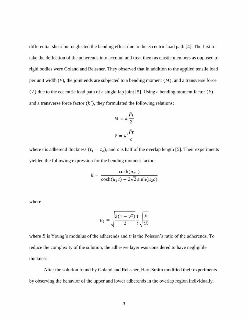
differential shear but neglected the bending effect due to the eccentric load path [4]. The first to

take the deflection of the adherends into account and treat them as elastic members as opposed to

rigid bodies were Goland and Reissner. They observed that in addition to the applied tensile load

per unit width (�̅�), the joint ends are subjected to a bending moment (𝑀), and a transverse force

(𝑉) due to the eccentric load path of a single-lap joint [5]. Using a bending moment factor (𝑘)

and a transverse force factor (𝑘′), they formulated the following relations:

𝑀 = 𝑘�̅�𝑡

2

𝑉 = 𝑘′�̅�𝑡

𝑐

where t is adherend thickness (𝑡1 = 𝑡2), and 𝑐 is half of the overlap length [5]. Their experiments

yielded the following expression for the bending moment factor:

𝑘 = cosh(𝑢2𝑐)

cosh(𝑢2𝑐) + 2√2 sinh(𝑢2𝑐)

where

𝑢2 = √3(1 − 𝑣2)

2

1

𝑡√

�̅�

𝑡𝐸

where 𝐸 is Young’s modulus of the adherends and 𝑣 is the Poisson’s ratio of the adherends. To

reduce the complexity of the solution, the adhesive layer was considered to have negligible

thickness.

After the solution found by Goland and Reissner, Hart-Smith modified their experiments

by observing the behavior of the upper and lower adherends in the overlap region individually.

4

This introduced the adhesive layer into the solution and produced an enhanced expression for

Goland and Reissner’s bending moment factor:

𝑘 = (1 +𝑡𝑎

𝑡)

1

1 + ξ c +16

(ξ c)2

where 𝑡𝑎 is the adhesive thickness, ξ 2 =�̅�

𝐷, and 𝐷 is the adhereneds bending stiffness [5].

2.2 Finite Element Modeling of Lap Shear Tests

To simulate single-lap shear tests, numerical modeling represents a viable option. Finite

element method determines approximate solutions to partial differential equations (PDEs) and

applies the selected parameters to small elements known as finite elements throughout the entire

geometry of the object. When lap shear tests are simulated via finite element modeling, the

adhesive is assumed to provide cohesive tractions across the interface joint [5]. Previous models

have used two-dimensional plane-stress elements to represent the adherends. The contact zone

has been assumed to exhibit linear-elastic behavior until yielding occurs and once yielding

occurs, it exhibits isotropic hardening [6].

5

3. Experimental Approach

Testing was performed on specimens provided by Engineering Bonding Solutions, LLC.

Data collected from testing was used to compare the validity of the FE results. The provided

samples were developed to comply with the ASTM D1002 test method. The adherend

dimensions are shown in Figure 1, where 𝐿 is the length of the overlap region. The bond gap for

the provided samples ranges from 0.254 mm to 0.305 mm.

Figure 1: Specimen Dimensions

As stated by the ASTM D1002 standard test method, the grip area must be a 1 inch by 1

inch square and must be sufficiently tightened to prevent slipping during testing. The material

testing machine utilized for the single-lap shear experiments was an Instron equipped with a

50kN capacity load cell (Figure 2). The free crosshead speed for the testing machine was

maintained at 1.3 mm (0.05 in)/min. The adherend materials included aluminum, cold rolled

steel, and stainless steel. Although these three metals were tested, the focus of the simulations

and this thesis will be on the aluminum samples. Methacrylate adhesives of various chemical

compositions (SA1-30-MOD, SA10-100, and SA10-05) were used to adhere the metallic tabs.

6

Figure 2: Instron 50kN Electromechanical Load Frame

Upon completion of the experimental setup, the Instron machine is set to apply a tensile

load on the clamped sample and elongates the specimen until the adhesive experiences either

adhesive or cohesive failure, shown in Figure 3 below. To ensure that the adhesive bond

possesses desirable strength, it is crucial to observe not only when the adhesive layer fails but

also how it is failing. With the ruptured sample and a clear representation of how the adhesive

tends to fail, the data outputted by the Instron software was extracted and analyzed using

Microsoft Excel.

7

Examples of each failure mode found in the experimental results are presented below. As

can be observed, for adhesive failure, the chemical bonds at the adherend-adhesive interface

become weaker than the adhesive strength of the adhesive. This causes the residual adhesive to

remain on one surface of the joint only. During cohesive failure, the specimen fails along the

thickness of the ahesive layer. This is typically caused by insufficient overlap length or excessive

peel stresses [7]. In this case, the residual adhesive remains on both surfaces.

Figure 3: Cohesive and Adhesive Failure Modes

Figure 4: Mixed Mode Failure (Adhesive and Cohesive) Figure 5: Adhesive Failure

8

Figure 8: Initial Loading Figure 7: Bending Moment Figure 6: Adherend Failure

Adherend failure occurs due to in-plane stresses resulting from the direct load stresses

and bending stresses which are imposed due to the eccentric load path of the experiment [8]. In

this failure mode, the bond between the fibers in the adherends fails prior to the adhesive,

causing failure in the aherend as opposed to the adhesive layer (Figures 6, 7, and 8) .

9

Presented above is a summary of the experiments run in the MOMRG lab. Due to the

primary purpose of these experiments being for industry and for creating a marketable product,

the composition of each adhesive was not disclosed. As can be seen on each specimen composed

of metal-to-metal bonds, each adhesive which follows the ASTM D1002 standard is tested on

aluminum (AL), cold rolled steel (CRS), and stainless steel (SS). Each specimen analyzed with

the ASTM D5868 standard contained fiberglass reinforced plastic (FRP). The single base

methacrylate specimens were provided by Engineering Bonding Solutions, LLC and are known

as ACRALOCK structural adhesives. Some data for a small amount of these adhesives is

available through the ACRALOCK website. Since the mechanical properties of SA10-05 are

provided by the datasheet online and were known through personal inquiry of the customer, this

adhesive is chosen as the focus of this research.

Figure 9: Summary of Experiments

10

The adherend chosen for analysis is aluminum (Figure 10). The modulus of elasticity of

aluminum 6061-T6 is known to be 68.9 GPa. The Poisson’s ratio is 0.33. For the SA10-05

adhesive, the modulus of elasticity and Poisson’s ratio (provided by supplier) are 620 MPa and

0.48, respectively. When combined, an adhesive layer of SA10-05 with aluminum adherends is

expected to have shear strength of 17.2 – 20.7 MPa.

Figure 10: SA10-05 Specimen with AL Adherends

11

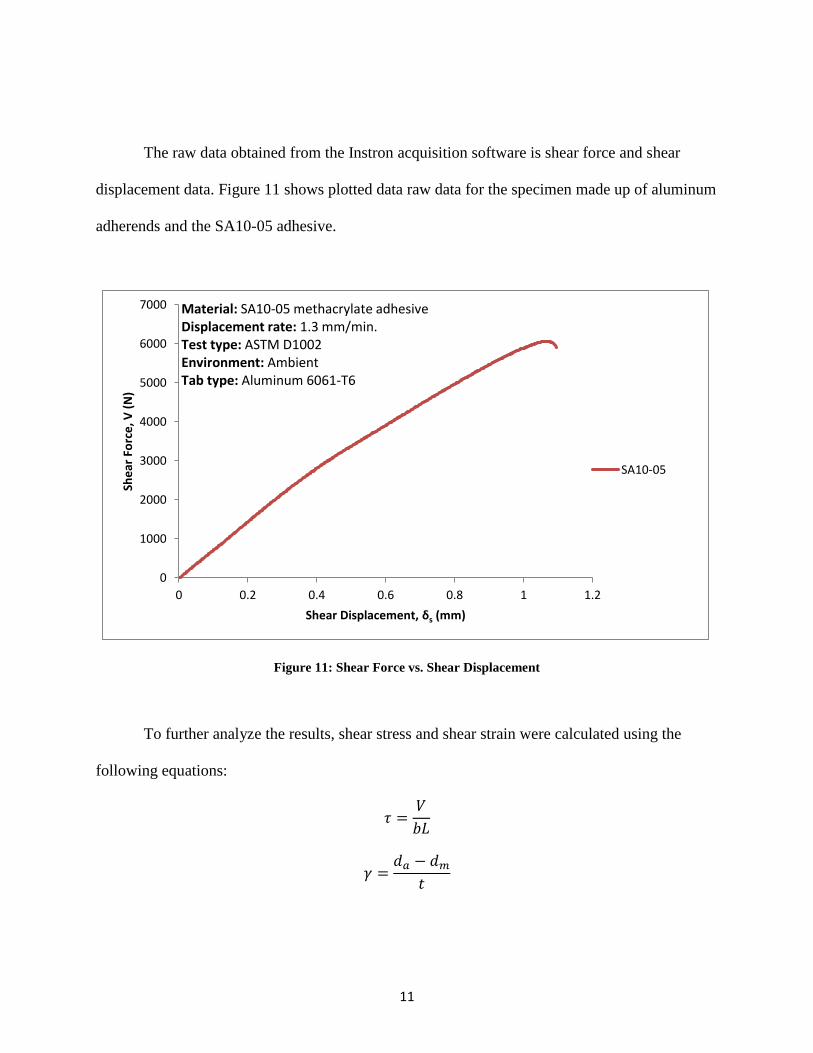
The raw data obtained from the Instron acquisition software is shear force and shear

displacement data. Figure 11 shows plotted data raw data for the specimen made up of aluminum

adherends and the SA10-05 adhesive.

Figure 11: Shear Force vs. Shear Displacement

To further analyze the results, shear stress and shear strain were calculated using the

following equations:

𝜏 =𝑉

𝑏𝐿

𝛾 =𝑑𝑎 − 𝑑𝑚

𝑡

0

1000

2000

3000

4000

5000

6000

7000

0 0.2 0.4 0.6 0.8 1 1.2

She

ar F

orc

e, V

(N

)

Shear Displacement, δs (mm)

SA10-05

Material: SA10-05 methacrylate adhesiveDisplacement rate: 1.3 mm/min.Test type: ASTM D1002Environment: AmbientTab type: Aluminum 6061-T6

12

where 𝜏 is engineering shear stress, 𝑉 is shear force, 𝑏 is the joint width, L is the joint length, 𝛾 is

engineering shear strain, 𝑑𝑎 is the displacement measured on the test sample, 𝑑𝑚 is the corrected

displacement of the adhered, and 𝑡 is the thickness of the adhesive layer [9]. Due to the nature of

this experiment, 𝑑𝑚 contributes a negligible amount of displacement and is therefore neglected.

The data curve for shear stress versus shear strain is shown below in Figure 12.

Figure 12: Shear Stress vs. Shear Strain

For the specific specimen in question, four trials were run. The data was collected for

each run and data analysis was conducted on the results. The collection of results is shown

below, in Figure 13.

13

Sample Width(mm) Length(mm) Area (mm^2)Load at

Failure (N)

Yeild Strength

(MPa)

Extension at

Failure (mm)

Strength at

Break

(MPa)

Failure (C/A)

1 25.4 12.7 322.586064.281359

18.79930981 1.09601 18.278427 COHESIVE

2 25.4 12.7 322.586218.509013

19.2774165 1.171575 18.334233 COHESIVE

3 25.4 12.7 322.585503.860776

17.06200253 1.1219942 15.698948 COHESIVE

4 25.4 12.7 322.585526.684519

17.13275627 1.0676128 15.545989 COHESIVE

Mean 25.4 12.7 322.58 5828.333917 18.06787128 1.114298 16.964399

St. Dev 0 0 0 367.0526664 1.137865542 0.044173314 1.5509535

COV 0 0 0 6.297728848 6.297728848 3.96422808 9.1424015

Figure 13: Collection of Experimental Data

14

Figure 15: INTER205 3-D 8-Node linear interface elements

4. Numerical Approach

4.1 Specimen Design

The finite element model developed in ANSYS uses three dimensional structural solid

elements, specifically SOLID185 eight-noded elements (Figure 14). Both the adherends and

adhesives were modeled utilizing this element type. To simulate the adhesion between the faces

of the adherends and the adhesive, eight-noded linear interface elements (INTER205) were used

(Figure 15). Using eight-noded elements as opposed to twenty-noded elements significantly

reduced both the complexity and solution time of the simulation.

Figure 14: SOLID185 3-D 8-Node structural solid elements

15

Due to the geometry of the model, it is convenient to use symmetry in order to further

reduce the complexity of the model. The number of elements was halved by mirroring the model

along the centerline of the y-axis, denoted in Figure 16 by a capital S. In a previous study

conducted by Kashif [10], it was found that the stresses and their gradients are high at or near the

ends of the overlap region. The critical regions are located at the adherend-adhesive interfaces

making it necessary to create a mesh with small elements across this area. This allows for

accurate solutions and employing this mesh refinement method through the thickness of the

specimen allows for the analysis of the stresses experienced through the thickness of the

adhesive. The level of refinement is shown in Figure 17.

16

Figure 16: Representation of Model Symmetry

17

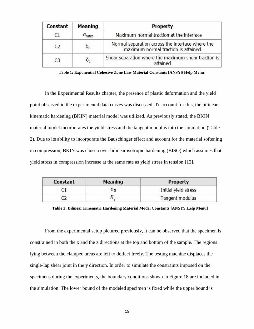
As previously mentioned, this finite element model utilizes the cohesive zone model

(CZM) to simulate the adhesive layer. In order to correctly create the interface elements required

by the cohesive zone approach, the elements along the xy-plane at the adherend-adhesive

interface must align perfectly. For this reason, a hexahedral mesh is used. The exponential law

for traction separation is followed, incorporating three material constants (Table 1). This

particular cohesive zone law is attractive to researchers because a phenomenological description

of contact is automatically achieved in normal compression and the tractions and their

corresponding derivatives are continuous [11].

Figure 17: Representation of Mesh Refinement

18

In the Experimental Results chapter, the presence of plastic deformation and the yield

point observed in the experimental data curves was discussed. To account for this, the bilinear

kinematic hardening (BKIN) material model was utilized. As previously stated, the BKIN

material model incorporates the yield stress and the tangent modulus into the simulation (Table

2). Due to its ability to incorporate the Bauschinger effect and account for the material softening

in compression, BKIN was chosen over bilinear isotropic hardening (BISO) which assumes that

yield stress in compression increase at the same rate as yield stress in tension [12].

From the experimental setup pictured previously, it can be observed that the specimen is

constrained in both the x and the z directions at the top and bottom of the sample. The regions

lying between the clamped areas are left to deflect freely. The testing machine displaces the

single-lap shear joint in the y direction. In order to simulate the constraints imposed on the

specimens during the experiments, the boundary conditions shown in Figure 18 are included in

the simulation. The lower bound of the modeled specimen is fixed while the upper bound is

Table 1: Exponential Cohesive Zone Law Material Constants [ANSYS Help Menu]

Table 2: Bilinear Kinematic Hardening Material Model Constants [ANSYS Help Menu]

19

allowed to translate freely in the y direction, accounting for the displacement induced by the

testing machine.

Figure 18: Boundary Conditions

20

4.2 Determining Material Constants

Each material model included in this simulation requires various material constants to be

inserted into the APDL code. In order to optimize the simulation and obtain accurate data, initial

guesses were chosen arbitrarily for each parameter. The simulation was run with these chosen

values and the data was stored. An iterative method, similar to the procedure used in a study

requiring traction-separation material parameters [13], in which each parameter was varied by

equal increments was then implemented to optimize the values. The results obtained from the

simulations were compared to the experimental data and modified until the simulation and the

experimental curves were considerably similar.

With the simulation curve possessing similar qualities as the experimental data curve, the

simulation parameter values were then varied further and inserted into a Taguchi array. An L25

orthogonal array was utilized to automate the iterative process, reducing the number of

experiments significantly. Table 3 shows how each experiment was determined, with 𝑃

representing a model parameter. Table 4 indicates the initial values used for the simulations and

Table 5 shows the varied values for each parameter.

21

Experiment 𝑷𝟏 𝑷𝟐 𝑷𝟑 𝑷𝟒 𝑷𝟓 𝑷𝟔

1 1 1 1 1 1 1

2 1 2 2 2 2 2

3 1 3 3 3 3 3

4 1 4 4 4 4 4

5 1 5 5 5 5 5

6 2 1 2 3 4 5

7 2 2 3 4 5 1

8 2 3 4 5 1 2

9 2 4 5 1 2 3

10 2 5 1 2 3 4

11 3 1 3 5 2 4

12 3 2 4 1 3 5

13 3 3 5 2 4 1

14 3 4 1 3 5 2

15 3 5 2 4 1 3

16 4 1 4 2 5 3

17 4 2 5 3 1 4

18 4 3 1 4 2 5

19 4 4 2 5 3 1

20 4 5 3 1 4 2

21 5 1 5 4 3 2

22 5 2 1 5 4 3

23 5 3 2 1 5 4

24 5 4 3 2 1 5

25 5 5 4 3 2 1

Table 3: Taguchi L25 Orthogonal Array

22

Parameters Initial Values

𝜎𝑚𝑎𝑥 (𝑀𝑝𝑎) 18.8

𝛿𝑛 (𝑚𝑚) 0.14

𝛿𝑡 (𝑚𝑚) 0.3

𝜎0 (𝑀𝑃𝑎) 16

𝐸𝑇 (𝑀𝑃𝑎) 80

𝐸 (𝑀𝑃𝑎) 620 Table 4: Initial Values for Taguchi Array

Parameters 1 2 3 4 5

𝜎𝑚𝑎𝑥 (𝑀𝑝𝑎) 18.8 14.1 16.45 21.15 23.5

𝛿𝑛 (𝑚𝑚) 0.14 0.105 0.1225 0.1575 0.175

𝛿𝑡 (𝑚𝑚) 0.3 0.225 0.2625 0.3375 0.375

𝜎0 (𝑀𝑃𝑎) 16 4 8 24 28

𝐸𝑇 (𝑀𝑃𝑎) 80 60 70 90 100

𝐸 (𝑀𝑃𝑎) 620 465 542.5 697.5 775

Table 5: Varied Values for Taguchi Array

23

5. Numerical Results

Prior to running the simulations, the values indicated by Table 5 were inserted into the

arrangement provided by the Taguchi L25 orthogonal array. Table 6 is the completed table with

all of the levels containing the parameter values tested.

Run 𝜎𝑚𝑎𝑥 (𝑀𝑝𝑎) 𝛿𝑛 (𝑚𝑚) 𝛿𝑡 (𝑚𝑚) 𝜎0 (𝑀𝑃𝑎) 𝐸𝑇 (𝑀𝑃𝑎) 𝐸 (𝑀𝑃𝑎)

1 18.8 0.14 0.3 16 80 620 2 18.8 0.105 0.225 4 60 465 3 18.8 0.1225 0.2625 8 70 542.5 4 18.8 0.1575 0.3375 24 90 697.5 5 18.8 0.175 0.375 28 100 775 6 14.1 0.14 0.225 8 90 775 7 14.1 0.105 0.2625 24 100 620 8 14.1 0.1225 0.3375 28 80 465 9 14.1 0.1575 0.375 16 60 542.5

10 14.1 0.175 0.3 4 70 697.5 11 16.45 0.14 0.2625 28 60 697.5 12 16.45 0.105 0.3375 16 70 775 13 16.45 0.1225 0.375 4 90 620 14 16.45 0.1575 0.3 8 100 465 15 16.45 0.175 0.225 24 80 542.5 16 21.15 0.14 0.3375 4 100 542.5 17 21.15 0.105 0.375 8 80 697.5 18 21.15 0.1225 0.3 24 60 775 19 21.15 0.1575 0.225 28 70 620 20 21.15 0.175 0.2625 16 90 465 21 23.5 0.14 0.375 24 70 465 22 23.5 0.105 0.3 28 90 542.5 23 23.5 0.1225 0.225 16 100 697.5 24 23.5 0.1575 0.2625 4 80 775 25 23.5 0.175 0.3375 8 60 620

Table 6: Completed L25 Taguchi Array

24

Each level of the Taguchi array was run for 100 time steps allowing enough points to be

collected to capture the behavior of the adhesive immediately before rupture. Examples of the

simulation data obtained from the Taguchi experiments are shown in Figures 19, 20, and 21

below.

Figure 19: Numerical Solution for Level 7

Figure 20: Numerical Solution for Level 10

0

2

4

6

8

10

12

14

0 0.5 1 1.5 2 2.5 3

She

ar S

tre

ss, τ

(M

Pa)

Shear Strain, γ (mm/mm)

L7 Taguchi

0

2

4

6

8

10

12

14

16

18

20

0 1 2 3 4

She

ar S

tre

ss, τ

(M

Pa)

Shear Strain, γ (mm/mm)

L10 Taguchi

25

Figure 21: Numerical Solution for Level 23

By noting the difference in values shown in the completed Taguchi array and observing

the data curves presented above, it is clear that even slight changes in the values of the

parameters alter the entire shape.

Along with the force and displacement output of the simulation, many other aspects of

the numerical solution were studied. In order to validate the simulation, results were compared to

findings in similar studies. The first portion of the verification process was the deflected shape of

the specimens immediately before rupture. Since it has been found that an eccentric load

imposed on a single-lap joint generates bending moment and transverse force [14] evidence of

adherend bending and adhesive debonding is expected. This phenomenon of rotating adherends,

first considered by Goland and Reissner in 1944, is illustrated in Figure 22. Figure 23 shows the

0

5

10

15

20

25

30

0 1 2 3 4 5

She

ar S

tre

ss, τ

(M

Pa)

Shear Strain, γ (mm/mm)

L23 Taguchi

26

deflected shape of a single-lap joint with a 0.254 mm adhesive layer thickness observed in a

previous study.

Figure 22: Rotating Adherends (Goland and Reissner, 1944)

Figure 23: Deformed Shape of Single-Lap Joint [8]

27

A comparison between what is found in literature and the results obtained from the FE

model presented here shows an agreement in the solutions. Figures 24 and 25 show the

undefelcted shape of the simulated specimen and the deformed shape immediately before

rupture, respectively.

Figure 24: Undeflected FE Model

Figure 25: Deflected FE Model

Knowing that the deflected shape resembles what is seen in literature, the comparison can

be expanded to include an analysis of the observations seen on the adherend- adhesive interface

and within the adhesive layer. Considering the nature of the single-lap shear experiment and the

geometry of the specimen, it is crucial that peel stresses be kept at a minimum to avoid

premature failure. To further validate the simulation, a study of the peel stresses experienced by

the upper interface of the adhesive and the adherend was conducted. When compared to what has

28

been found in prior studies, it is seen that the simulation produces peel stress data similar to what

is expected from a single-lap specimen. Figures 26 and 27 show the peel stress distribution

found in literature and the simulation data, respectively.

Figure 26: Peel Stress Distribution [10]

Figure 27: Simulation Peel Stress Distribution

29

6. Comparing Numerical and Experimental Solutions

With the assurance that the simulation was providing reasonable results, considerable

effort was put into obtaining simulation data which closely matched the experimental data. Since

a collection of data from simulations run for each level of the Taguchi array was present, the

simulation data was plotted on the same axis as the experimental data for each run (Figures 28,

29, and 30).

Figure 28: Comparison Between Experimental and L7 Simulation Data

0

2

4

6

8

10

12

14

16

18

20

0 1 2 3 4

She

ar S

tre

ss, τ

(M

Pa)

Shear Strain, γ (mm/mm)

Experimental

L7 Taguchi

30

Figure 29: Comparison Between Experimental and L10 Simulation Data

Figure 30: Comparison Between Experimental and L23 Simulation Data

0

2

4

6

8

10

12

14

16

18

20

0 1 2 3 4

She

ar S

tre

ss, τ

(M

Pa)

Shear Strain, γ (mm/mm)

L10 Taguchi

0

5

10

15

20

25

30

0 1 2 3 4 5

She

ar S

tre

ss, τ

(M

Pa)

Shear Strain, γ (mm/mm)

Experimental

L23 Taguchi

31

Considering every level of the Taguchi array and the results obtained from each, it is

obvious that level 10 provides the most accurate solution (Figure 29). The initial slope (elastic

modulus) for the elastic region matches the experimental data curve closely. Upon reaching the

yield stress and entering the region where plastic deformation occurs, a similar tangent modulus

is found between both curves. As the specimen approaches the point of rupture, the experimental

data and the simulation data both reach their ultimate strengths at approximately 18.8 MPa.

Throughout the numerical simulation procedure, a trend was seen where iterations were

performed until the parameters were optimized. This method, although effective, is tedious and

requires an extensive amount of time. In order to reduce experiment time and make the process

more convenient, mathematical models were developed with respect to 𝜏 and the other with

respect to 𝛾.

𝜏 =𝛾

𝛿𝑠+ 𝛾𝜎𝑚𝑎𝑥𝛿𝑛 +

𝛾𝜎𝑚𝑎𝑥𝛿𝑛𝛿0 − 𝜎𝑚𝑎𝑥𝛿𝑠𝛾3

𝐸𝑇

𝛾 =𝜏𝛿𝑠

(𝛿𝑠𝐸𝑇 + 𝜎𝑚𝑎𝑥𝛿𝑠𝛿0 − 𝜏)𝛿𝑛

Below, the curves obtained from the mathematical models, the simulation curves, and the

experimental data are plotted on the same axis for three selected Taguchi levels (Figures 31, 32,

and 33). Although the ultimate goal of the mathematical modeling effort is to obtain an equation

which fits the elastic and plastic regions, along with the rupture, it can be seen that the

mathematical models do follow the data quite well. Through the use of these equations, estimates

32

of the cohesive zone and bilinear kinematic hardening models can be obtained. These values can

be used to significantly reduce the time necessary to obtain an accurate numerical solution.

Figure 31: Experimental, Numerical, and Mathematical Modeling Curves for L7

Figure 32: Experimental, Numerical, and Mathematical Modeling Curves for L10

33

Figure 33: Experimental, Numerical, and Mathematical Modeling Curves for L23

34

7. Conclusions

The goal of this research is to provide a method to numerically understand the

mechanical properties of adhesives. Through the use of FEA simulations, numerical results for

single-lap shear tests were obtained and compared to experimental data. By doing so and

comparing to results found in literature, the model was validated and it was assured that accurate

results were being acquired. The FEA model made use of the cohesive zone method (CZM) to

model the adhesive layer. In order to account for the yield stress and the plastic deformation, the

bilinear kinematic hardening (BKIN) material model was employed. By implementing these

modeling techniques, creating a mathematical model utilizing the simulation data and comparing

each result, a valid approach to observe the behavior of single-lap joints is created and the

mechanical properties of adhesive layers are thoroughly explored to better understand adhesive

bonding and optimize bond strength.

35

Appendix

36

finish

/clear

/PNUM,TYPE,1

/title, Tensile Test Redo

/prep7

ET,1,SOLID185

ET,2,SOLID185

ET,3,SOLID185

MP,EX,1,6.9E4 ! Young's modulus (Material 1 - N/mm^2)

MP,PRXY,1,0.334 ! Poisson's ratio (Material 1)

MP,EX,2,620

!MP,GXY,2,21.692 ! Young's modulus (Material 2 - N/mm^2)

MP,PRXY,2,0.48

TB,BKIN,2

TBDATA,,4,60 !BKIN

MP,EX,3,6.9E4 ! Young's modulus (Material 3 - N/mm^2)

!MP,GXY,3,2.4E4 ! Shear Modulus (N/mm^2)

MP,PRXY,3,0.334

TYPE,1

BLOCK,0,12.7,0,-101.6,0,1.6

Mat, 1

mshape,0,3D ! Differentiate between Textra- and Hexa-

TYPE,1

LESIZE,7,,,8

LESIZE,11,,,2

LESIZE,6,,,136

VMESH,1

DA, 6,SYMM

TYPE,2

BLOCK,0,12.7,-88.9,-101.6,1.6,1.9

37

Mat,2

TYPE,2

LESIZE,18,,,17

LESIZE,22,,,3

LESIZE,19,,,8

VMESH,2

DA, 12,SYMM

TYPE,3

BLOCK,0,12.7,-88.9,-190.5,1.9,3.5

Mat,3

TYPE,3

LESIZE,29,,,8

LESIZE,34,,,2

LESIZE,30,,,136

VMESH,3

DA, 18,SYMM

ESEL,S,TYPE, ,2

NSLE

NSEL,R,LOC,Y,-88.9,-101.6

CM,ADH1,NODE,

NSEL,S,LOC,Y,0

CM,TOP_1,ELEM,

NSEL,S,LOC,Y,0

CM,TOP1,NODE,

ESEL,S,TYPE,,1

NSEL,R,LOC,Y,0

NSEL,R,LOC,X,0

CM,TOPSING,NODE

ESEL, S, TYPE, ,3 !Select a subset of elements

NSLE !Select nodes associated with above elements

NSEL,R,LOC,Y,-101.6

38

CM, TOP3, NODE,

NSEL, S, LOC, Y, -190.5

CM, BASE3, NODE,

ALLSEL,ALL

TNMAX=23.5

delta_norm=0.175

delt_shear=0.3375

ET,4,INTER205

TB,CZM,4,,,EXPO

TBDATA,1,TNMAX,delta_norm,delt_shear

CSYS,0

esel,s,type,,2

NSEL,R,LOC,Y,-88.9,-101.6

NSEL,R,LOC,X,12.7

!NSEL,R,LOC,Z,1.6,2.1

CM,SIDE,NODE,

ALLSEL,ALL

!***************************************************

ESEL, S, TYPE, ,1,

CM, ePlate1, Elem

ESEL, S, TYPE, ,2,

CM, ePlate2, Elem

ESEL, S, TYPE, ,3,

CM, ePlate3, Elem

ESEL, S, TYPE, ,1,2,1

NSLE

NSEL, S, LOC, Y, -88.9,-101.6, 1

NSEL, R, LOC, Z, 1.6,

NUMMRG,Nodes

Type,4

MAT,4

CZMESH, ePlate1, ePlate2,

------------------------------------------

39

ESEL, S, TYPE, ,2,3,1

NSLE

NSEL, S, LOC, Y, -88.9,-101.6, 1

NSEL, R, LOC, Z, 1.9,

NUMMRG,Nodes

Type,4

MAT,4

CZMESH, ePlate2, ePlate3,

!NSEL,S,LOC,Y,-101.6

!NSEL,R,LOC,Z,2.1,3.7

!NUMMRG,NODES

!ESLN

!NSEL,S,LOC,Y,-88.9

!NSEL,R,LOC,Z,0,1.6

!NUMMRG,NODES

!ESLN

!********************Boundary Conditions***********************

!cmsel,s,ADH1,NODE

!D,ALL,UZ,0

!D,ALL,UY,0

!D,ALL,UX,0

!cmsel,s,ADH2,NODE

!D,ALL,UZ,0

!D,ALL,UY,0

!D,ALL,UX,0

cmsel, s, top1, node

D,ALL,UZ,0

D,ALL,UX,0

cmsel, s, base3, node

D,ALL,UZ,0

D,ALL,UY,0

D,ALL,UX,0

40

allsel,all

/SOLU

ANTYPE,STATIC

NLGEOM,ON

cmsel, s, top1, node

!CP,NEXT,UY,ALL

!F,ALL,FY,100

D,top1,UY,1.3

ALLSEL, ALL

!TIME,20

sub_steps = 10

AUTOTS,OFF

NSUBST, sub_steps

Outres, All, All

solve

FINISH

!/EXPAND,2,RECT,HALF,12.7

!/REPLOT

!******POSTPROCESSEING******************

!*DIM,TTime,ARRAY,TIME_count,1

/post1

/OUTPUT,WithoutBKIN,txt,C:\Users\Wilson\Desktop\Research\Results\New_Test

!*DIM,ReactionForces,ARRAY,sub_sets

RESET

cmsel,s,top1,node

NPLOT

*DO,i,0,sub_steps,1

SET,,, ,,, ,i

FSUM,,top1

!PRRSOL,FY

*ENDDO

/post1

/OUTPUT,Stress_stuff,txt,C:\Users\Wilson\Desktop\Research\Results

RESET

NSEL,S,LOC,Y,-88.9,-101.6

41

NSEL,R,LOC,Z,2.1

NSEL,R,LOC,X,0

NPLOT

*DO,i,0,sub_steps,1

SET,,, ,,, ,i

!PLNSOL, S,EQV, 0,1.0

PRNSOL,EPTO,PRIN

*ENDDO

/post1

/OUTPUT,Stress_stuff,txt,C:\Users\Wilson\Desktop\Research\Results

NSEL,S,LOC,Y,-88.9,-101.6

NSEL,R,LOC,Z,1.8

NSEL,R,LOC,X,0

NPLOT

SET,,, ,,, ,19

!*

PRNSOL,S,PRIN

/post1

/OUTPUT,Stress_stuff,txt,C:\Users\Wilson\Desktop\Research\Results

NSEL,S,LOC,Y,-88.9,-101.6

NSEL,R,LOC,Z,1.8

NSEL,R,LOC,X,0

NPLOT

SET,,, ,,, ,19

!*

PRESOL,S,PRIN

!*****************************************************************************

42

References

[1] Albuquerque, E., Paiva, W., Rodrigues, M., and Rodriguez, R., 2010, “Analytical and

Numerical Tools for Bonded Joint Analysis,” Mecánica Computacional, 29, pp. 7557-

7569.

[2] Alía, C., Arenas, J., and Narbón, J., “Optimum Adhesive Thickness in Structural Adhesives

Joints Using Statistical Techniques Based on Weibull Distribution,” pp. 1-6.

[3] Brown, K., Carbas, R., Critchlow, G., Figueiredo, M., and da Silva, L., 2009, “Effect of

Material, Geometry, Surface Treatment and Environment on the Shear Strength of Single

Lap Joints,” International Journal of Adhesion & Adhesives, 29 (6), pp. 621-632.

[4] Christensen, T., 1976, “A Finite Element Analysis of a Single Lap Shear Adhesive Joint With

and Without an Edge Crack,” pp. 48-65.

[5]Court, R., Sutcliffe, M., and Tavakoli, S., 2001, “Ageing of Adhesively Bonded Joints –

Fracture and Failure Analysis Using Video Imaging Techniques,” International Journal

of Adhesion and Adhesives, 21 (6), pp. 2-3

[6] Kafkalidis, M., and Thouless, M., 2002, “The Effects of Geometry and Material Properties on

the Fracture of Single Lap-Shear Joints,” pp. 8-18.

[7] Davis, M.J., and Bond, D.A., “The Importance of Failure Mode Identification in Adhesive

Bonded Aircraft Structures and Repairs,” Aircraft Structural Integrity Section.

[8] Zhu, Y., and Kedward, K., 2005, “Methods of Analysis and Failure Predictions for

Adhesively Bonded Joints of Uniform and Variable Bondline Thickness,” Technical

Report No. DOT/FAA.AR-05/12, Federal Aviation Administration, Washington, DC.

43

[9] ASTM D5656-10, Standard Test Method for Thick-Adherend Metal Lap-Shear Joints for

Determination of the Stress-Strain Behavior of Adhesives in Shear by Tension Loading,

ASTM International, West Conshohocken, PA, 2010,www.astm.org

[10] Kashif, S.M., (0017), “Delamination effect modeling, simulation and experimental

validation of lap shear test,” International Journal of Mechanical and Materials

Engineering.

[11] Bosch, M.J., Schreurs, P.J.G., Geers, M.G.D., 2006, “An improved description of the

exponential Xu and Needleman cohesive zone law for mixed-mode decohesion,”

Engineering Fracture Mechanics, 73, pp. 1220-1234

[12] Taneja, A., 2012, “On isotropic and kinematic hardening,” http://www.ajaytaneja-

isotropickinematichard.blogspot.com/

[13] Di Leo, C.V., Luk-Cyr, J., Liu, H., Loeffel, K., Al-Athel, K., Anand, L., 2014, “A new

methodology for characterizing traction-separation relations for interfacial delamination

of thermal barrier coatings,” Acta Materialia, 71, pp. 306-318

[14] Moreira, D.C., Nunes, L.C.S., 2014, “Experimental analysis of bonded single lap joint with

flexible adhesive,” Applied Adhesion Science, 2, pp. 1-8