Compnfm & SlmcIuns Vol. 15. No. 5. pp. 533-54. 1982 0045-7919/82/050J333.~/0 Ptiied in Gnat Britain. Pcrgamon Press Ltd.

FINITE-ELEMENTTECHNIQUEFORSOLVING PROBLEMSFORMULATEDBY HAMILTON'S PRINCIPLE

S. SOREK and J.J. BLECHt Faculty of Mechanical Engineering, Technion-Israel Institute of Technology, Haifa, Israel

(Received 23 January 1981; received for publication 26 August 1981)

Abrtnct-The finite element technique is applied to functionals which govern dynamical problems, where time is an independent variable.

The present paper demonstrates improved accuracy in mass-spring-damper systems and exemplifies “rendevous problems” of a “travelling” particle in a medium. The motion is governed by Hamilton’s principle. The time interval is tixed.

Functionals are constructed from Hamilton’s extended principle and appropriate conditions stating the various constraints.

Initial value problems may be incorporated by writing a functional in accordance with Gurtin’s method. Shape functions are polynomials in time and can be extended to other spatial variables when present. As a result of a variation to the functional, a system of algebraic (not necessarily linear) equations is formed.

This system is solved simultaneously to yield its motion within the boundaries of the given time interval.

Abbreviations NOMENCLMVRE

CFS HPFE

KKS SFFE

VP

B t

to4 T V

5Y

closed form solution Hamiliton’s principle with finite elements Runge-Kutta’s solution second functional with finite elements velocity’s power

time derivation vector elements independent parameters at the nodes that belongs to an element element’s nodes convolution product variational operator time step damping coefficient nonconservative external force impulse gravity acceleration spring coefficient the Lagrangian; L = T - V mass shape function power of particle’s velocity when introduced in

Hamilton’s principle; 1= l/2 (VP-l) generali.zed coordinate particle’s velocity time time limits at the origin and final time interval system’s kinetic energy system’s potential energy coordinates

Gnek symbols I functional 7 normalized time 0 natural frequency O, specific damping coefficient; 01 = B/m

tFaculty of Mechanical Engineering, Technion, Israel Institute of Technology; Haifa, Israel.

INTRODUCTION

In a finite element analysis for time dependent phenomena, a variation is usually applied to the spatial approximations of the dependent variables [l-3], yielding a system of ordinary differential equations in time which yield an initial value problem. Solutions to such systems are well documented.

Fried[4] used Hamilton’s principle to develop a pro- cedure which can be regarded as a generalization of the step-by-step method for integrating the dynamic equation of motion. Vance and Sitchin[S] received a system of recurrence equations using the finite differences method, and by imposing Lagrange multipliers into Hamilton’s principle.

Papers dealing with the question of whether Hamil- ton’s principle is an extremum principle, were presented by Leitmann[6], Smith, D. R. and Smith, C. V.[7]. Gurtin in his papers [8,9] extended the application of variational method by showing how initial conditions may be in- corporated explicitly in the variational formulation of a problem, the limitation of his method being that only linear problems can be dealt with. Sandhu and Wilson[lO] had applied the finite element method to functionals of Gurtin’s method for fluid flow in porous media.

The present method includes the time variable in the functional to be varied. Boundary conditions at both ends of the time interval are given. The entire time interval (the only independent variable at the present work) is also a given parameter.

Applying the finite element technique to a given functional, a differential formulation, that of searching an extremum to a function of several variables is obtained.

In contrast to initial value problems techniques, here a system of algebraic equations is derived from Hamil- ton’s extended principle. The system is solved simul- taneously. This fact prevents an accumulation of round- off errors.

Various constraints, when present, are imposed as

533

534 S. SOREK and J. J. BLECH

appropriate additions to corresponding equations of the system.

An example showing an application of the present method to a Gurtin type functional will be shown later on.

For some examples that were illustrated, a comparison was made between: (1) the closed form solution; (2) a solution based on the Runge-Kutta method; (3) a solu- tion derived from a functional not identical to Hamilton’s extended principle.

For the problems that were solved it was demonstrated that applying the finite element method to Hamilton’s principle (being a stationary principle) gives better cor- relation to the closed form solution than using either the Runge-Kutta method, or the solution which was generated in Step (3) above.

The work done here is based on the M.Sc. research thesis of the first author [ll] which was performed during the year 1975.

DYNAMICAL SYSTEMS

Hamilton’s extended principle states that [5]:

noting that the variation is not applied to non-con- servative external forces [12]. Equation (l), due to the fact that not all of its parts underwent a variation, is not an extremum of J. Adding the expression, _f(Zf&)dt, Hamilton’s extended principle may be regarded as a vir- tual work principle.

Leitmann[6] presented for certain types of field differential equations, functionals such that when varia- tion is applied to all of their expressions the field equa- tions result. A finite element desecretization for ap- proximating generalized coordinates in the element would be:

(2)

Two degrees of freedom at each element’s node yields:

qi?’ =]qj* @+I, 6, &+tlT. (3)

Normalizing shape functions so that each one equals unity at the correspondent element’s node and zero at the second node, yields third degree polynomials:

NE = IN,, N2, N, N,, NAT

= [(I -3T2+ 2T3), (3T2_2T3),

A& - T)‘, - Af12( 1 - T)] = (4)

AE=tj+l-tj; T=?. E

Inserting the finite element desecretization into the functional yields a function with several independent variables, as many as the number of degrees of freedom which are imposed on element’s nodes. For two degrees of freedom, we have:

.r = .I(qk, dk, t)* (5)

Proceeding with the variation, a formulation that of searching an extremum is obtained:

(6)

by which a system of algebraic equations is formed.

ILLUSTRATIVE EXAMPLES

(1) Mass spring and damper system The functional in accordance to Hamilton’s extended

principle would be:

J,=fm6[f2- 02x2 - (20, i)x] df. (7)

Not using Hamilton’s principle a second accurate func- tional would be [7]:

J2=im I *f e”“(P - 02x2)dt. (8 :il

Following eqns (5) and (a), with finite element de- scretization, a system of two algebraic equations for each element’s node (k) would then be:

(3,=4 [k’x=(k’ - o,N=)

- 02NTx’NT] $- dr = 0 t

I (9)

($),=AEI, fiTxe(IiT - o,N=)

- 02NTx’NT] dx’dT,O ai

k I and for the second functional:

- 02NTxeNT)$dr = 0 k

I (10)

- W2NTxeNT)$dr = 0. k

Letting j = k and j = k - 1 intermittently, yields a system of linear algebraic equations that involve parameters aboutnodesk-l,k,ktl.

Integrating the recurrence system formed by Hamil- ton’s extended principle, eqns (9), and letting:

A=AB=tk-tk_,=tk+,-tk;AeQl

yields:

=&+,-2&t&+,=0 (11)

Finite-element technique for solving problems formulated by Hamilton’s principle 535

= &+, -&., = 0. (12)

Multiplying eqn (12) by f yields the Taylor expansion for xk+, and &-1 as functions of parameters about the node k.

.&A = $(&+, - xk-,) &A= = xk-1 -2x, t &+, I

(13)

Equations (13) are used as finite difference schemes that stand for the appropriate expressions in the equations of motion.

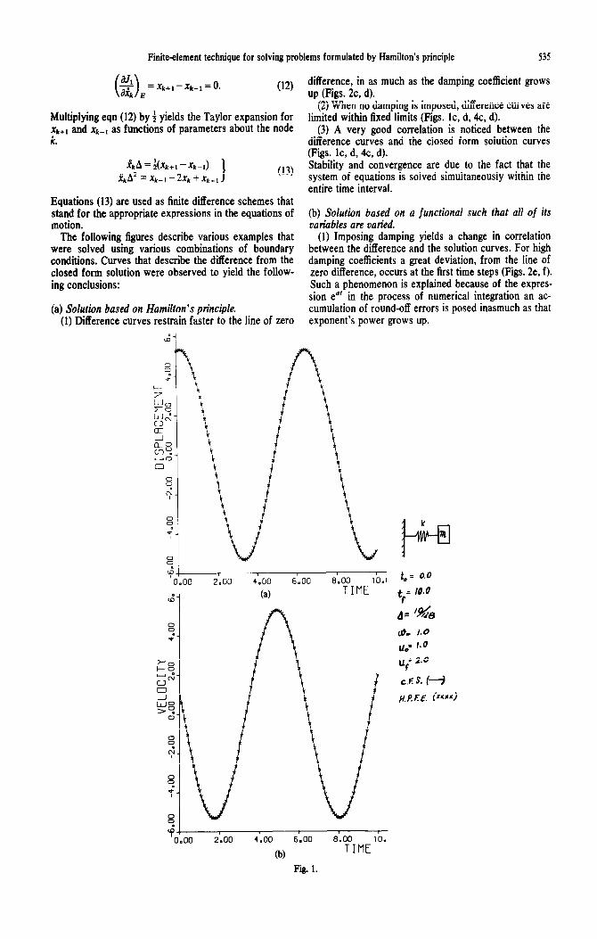
The following figures describe various examples that were solved using various combinations of boundary conditions. Curves that describe the difference from the closed form solution were observed to yield the follow- ing conclusions:

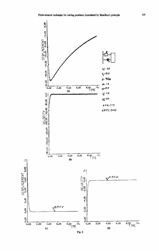
(a) Solution based on Hamilton’s principle. (1) Difference curves restrain faster to the line of zero

difference, in as much as the damping coefficient grows up (Figs. 2c, d).

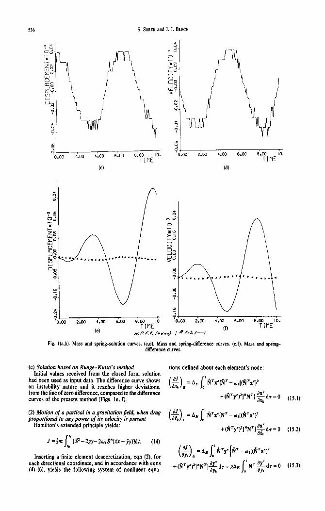
(2) When no damping is imposed, difference curves are limited within fixed limits (Figs. lc, d, 4c, d).

(3) A very good correlation is noticed between the difference curves and the closed form solution curves (Figs. lc, d, 4c, d). Stability and convergence are due to the fact that the system of equations is solved simultaneously within the entire time interval.

(b) Solution based on a functional such that all of its variables are varied.

(1) Imposing damping yields a change in correlation between the difference and the solution curves. For high damping coefficients a great deviation, from the line of zero difference, occurs at the first time steps (Figs. 2e, f). Such a phenomenon is explained because of the expres- sion eat in the process of numerical integration an ac- cumulation of round-off errors is posed inasmuch as that exponent’s power grows up.

+oti * D 4.00 L = 6.00 8.00 ,b., to 0.0

2’1 (a) TIME $S 10.0

‘PA 0.00 2.00 4.00 6.00 8.00 IO.

(b) TIME

Fii. 1.

536 S. SOREK and J. J. BLECH

44 0.00 2.00 4.00 6.00 a.00 IO.

TIME (4

,.

8.00 IO, TIME

(4

4 0.00 2.00 4.00 6.00 8.00 10.

tn TIME w H.P.F.E. /urrr) / R-0. /-) ‘-’

Fig. l(a,b). Mass and spring-solution curves. (c,d). Mass and spring4ifference curves. (e,f). Mass and spring difference curves.

(c) Solution based on Runge-Kutta’s method. tions defined about each element’s node: Initial values received from the closed form solution

had been used as input data. The difference curve shows an instability nature and it reaches higher deviations, (EL=AEl,

rVx+J= - o,[($X’)*

from the line of zero difference, compared to the difference curves of the present method (Figs. le, f). +(kTye)‘]“N’}~dr=O (15.1)

(2) Motion of a partical in a gravitation field, when drag proportional to any power of its velocity is present ($9, =AEl, $x={N= - ~,[(fi=x=)*

Hamilton’s extended principle yields: + (fi’y’)*]“NT}~ dr = 0 (15.2)

J=im I

’ 19” - 2gy- 2w,9’73x + jy)]dt. (14) CO

Inserting a finite element desecretization, eqn (2), for ($), = be 1.’ firy’(kT - ~,[(fi~x’)*

each directional coordinate, and in accordance with eqns (4)-(6), yields the following system of nonlinear equa-

+ &‘y’)‘]‘NT}~ dr = gA,, \’ NT $$ dr = 0 (15.3) 0

I-

S. SOREK and J. J. BLECH

4.00 (o)

6.00 8.00 10. t 00 2.00 4.00 6.00 6.00 IO. TIME (9 TIME

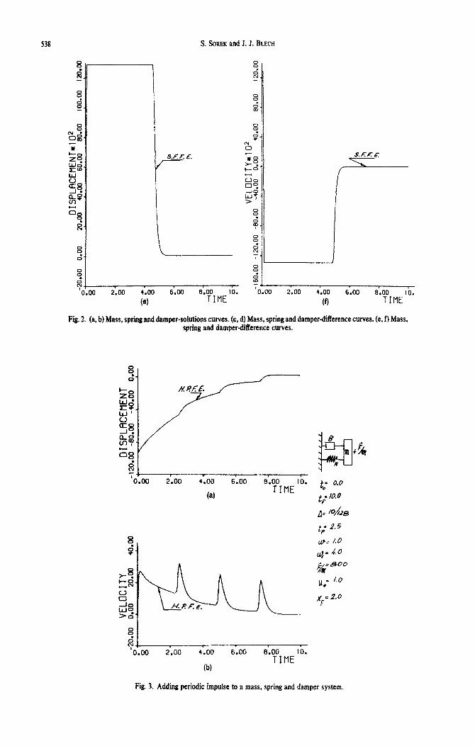
Fii 2. (a, b) Mass, spring and dam~r-soi~~ns curves. (c, d) Mass, spring and dam~r~ifferen~ curves. (e, f) Mass, spring and damper-difference curves.

8 . B+ '0.00 2.00 4.00 6.00 8.00 IO.

TIME 04

Fig. 3. Adding periodic impulse to a mass, spring and damper system.

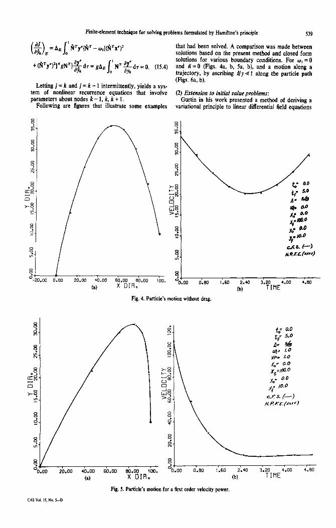
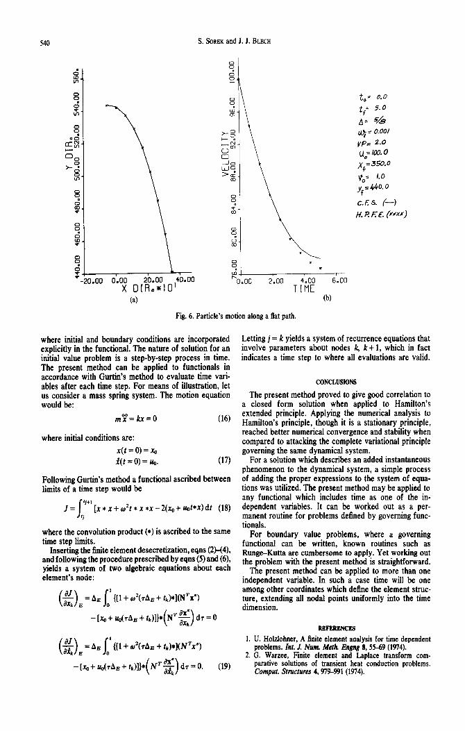
Finiteclement technique for solving problems formulated by Hamilton’s principle 539

rVy’{IV - o*[(rVX’)2 that had been solved. A comparison was made between solutions based on the present method and closed form

+ Rj’y’)‘]“gN=}~ I

I solutions for various boundary conditions. For o1 = 0

ah dr = gA, NT x dT = 0. (15.4)

ayk

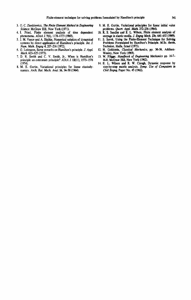
and fi = 0 (Figs. 4a b, Sa, b), and a motion along a 0 trajectory, by ascribing J/ye 1 along the particle path

Letting j = k and j = k - 1 intermittently, yields a sys- (Figs. 6a, b).

tem of nonlinear recurrence equations that involve parameters about nodes k - 1, k, k + 1.

(2) Extension to initial value problems:

Following are figures that illustrate some examples Gurtin in his work presented a method of deriving a

variational principle to linear differential field equations

z--- . . 20.00 40.00 60.00 80.00 100. 0

(a) x DIR.

I

\

-r- 0.c m 0;eo 1;60 2;40 3;20 4;oo 4;eo

0) TINE

Fig. 4. Particle’s motion without drag.

. DO 20.00 40.00 60.00 60.00 100. "0.00 0.60 1.60 2.40 3.20 4.00 4.80

(a) x DIR. 0) TIME

Fig. 5. Particle’s motion for a first order velocity power.

CAS Vol. 15. No. 5-D

540 S. SOREK and J. J. BLECH

to= 0.0

t,: 5.0

A= 5h

(q - 0.001

yps 2.0 uo= ILV. 0

/y,=Jso.O

vo= 1.0

yf=440.0

c.Es. (-1

H. J? EE. (~~~~)

(4 TIME

(f-9

Fig. 6. Particle’s motion along a flat path.

where initial and boundary conditions are incorporated explicitly in the functional. The nature of solution for an initial value problem is a step-by-step process in time. The present method can be applied to functionals in accordance with Gurtin’s method to evaluate time vari- ables after each time step. For means of illustration, let us consider a mass spring system. The motion equation would be:

m?=kx=O (16)

where initial conditions are:

x(t = 0) = XIJ i(t = 0) = uo. (17)

Following Gurtin’s method a functional ascribed between limits of a time step would be

J= I

‘+’ [x * x t 02t * x *x -2(x, t uot*x) dt (18) *i

where the convolution product (*) is ascribed to the same time step limits.

Inserting the 6nite element desecretization, eqns (2)-(4), and following the procedure prescribed by eqns (5) and (6), yields a system of two algebraic equations about each element’s node:

(3, =A4 {[l t 02(7AE t &)*](NTx’)

-[G t d7AE t l,)]}*(Nrg) d7 = 0

63, =A4 {[l + 02(7AB t t,)*](N%‘)

-[x&,,(rP,+~,‘)]}*(Nr$)d~=O. (19)

Letting j = k yields a system of recurrence equations that involve parameters about nodes k, k t 1, which in fact indicates a time step to where all evaluations are valid.

CONCLUSIONS

The present method proved to give good correlation to a closed form solution when applied to Hamilton’s extended principle. Applying the numerical analysis to Hamilton’s principle, though it is a stationary principle, reached better numerical convergence and stability when compared to attacking the complete variational principle governing the same dynamical system.

For a solution which describes an added instantaneous phenomenon to the dynamical system, a simple process of adding the proper expressions to the system of equa- tions was utilized. The present method may be applied to any functional which includes time as one of the in- dependent variables. It can be worked out as a per- manent routine for problems defined by governing func- tionals.

For boundary value problems, where a governing functional can be written, known routines such as Runge-Kutta are cumbersome to apply. Yet working out the problem with the present method is straightforward.

The present method can be applied to more than one independent variable. In such a case time will be one among other coordinates which define the element struc- ture, extending all nodal points uniformly into the time dimension.

REFERENCES

1. U. Holzlohner, A linite element analysis for time dependent problems. Znt. 1. Num. Meth. Engng 8,5%9 (1974).

2. G. Warzee, Finite element and Laplace transform com- parative solutions of transient heat conduction problems. Comput. Structures 4,979-991 (1974).

Finite-element technique for solving problems formulated by Hamilton’s principle 541

3. 0. C. Zienkiewicz, The Finite Element Method in Engineering 9. hf. E. Gurtin, Variational principles for linear initial value Science. McGraw Hill, New York (1971). problems. Quart. Appl. MaM 252256 (1964).

4. I. Fried, Finite element analysis of time dependent 10. R. S. Sandhu and E. L. Wilson, Finite element analysis of phenomena. AZAA .I. 7(6), 1170-I 173 (1%9). seepage in elastic media. .r. Engng Mech. Dfu. 641652 (1969).

5. J. M. Vance and A. Sitchin, Numerical solution of dynamical 11. S. Sorek, Using the Finite-Element Technique for Solving systems by direct applicatton of Hamilton’s principle. Int. 1. Problems Formulated by Hamilton’s Principle. M.Sc. thesis, Num. Meth. Engng 4,207-216 (1972). Technion, Haifa, Israel (1975).

6. G. Leitmann, Some remarks on Hamilton’s principle. J Appl. Mech. 623425 (1973).

7. D. R. Smith and C. V. Smith, Jr., When is Hamilton’s principle an extremum principle? AIAA J. 12( I l), 157>1576 (1974).

8. M. E. Gurtin, Variational principles for linear elastody- namics. Arch. Rat. Mech. Anal. 16, 34-50 (1964).

12. H. Goldstein, Clnssical Mechanics, pp. 3&56, Addison- Wesley, New York (1969).

13. W. Flugge, Handbook of Engineering Mechanics pp. S-7- 16-8, McGraw Hill, New York (1%2).

14. E. L. Wilson and R. W. Clough, Dynamic response by step-by-step matrix analysis. Symp. Use oj Compufers in Civil Engng, Paper No. 45 (1%2).