FINITE-ELEMENTMODELLING OF - AudiLab home pageaudilab.bme.mcgill.ca/~funnell/AudiLab/theses/siah_2002_thesis.pdf · 4.2.2 The variational method 17 ... CHAPTER6 FINITE-ELEMENTMODEL

•

•

•

FINITE-ELEMENT MODELLING OFTHE MECHANICS OF THE COUPLING

BETWEEN THE INCUS AND STAPES INTHE MIDDLE EAR

Tiong Reng Siah

A thesis submitted to the Faculty of Graduate Studies and

Research in partial fulfi1ment of the requirements of the degree of

Master of Engineering

Department of Electrical & Computer Engineering

McGill University

Montréal, Québec

March2002

© Tiong Reng Siah, 2002

1+1 National Libraryof Canada

Acquisitions andBibliographie Services

38S Wellington St,..tOftawa ON K1 A 0N4canada

BibliothèQue nationaledu Canada

Acquisitions etserviees bibliographiques

395. rue w..ngton0Ita_ ON K1A 0N4Canada

The author bas granted a nonexclusive licence allowing theNational Libnuy ofCanada tareproduce, loD, distnbute or sencopies of this thesis in microform,paper or electronic formats.

The author retains ownershïp ofthecopyright in this thesis. Neither thethesis nor substBntial extracts from itmay he printed or otherwisereproduced without the author'spem11SS1on.

L'autem a accordé une licence nonexclusive permettant à laBibliothèque nationale du Canada dereproduire, pr~, distribuer ouvendre des copies de cette thèse sousla forme de microfichelfilm, dereproduction sur papier ou sur fonnatélectronique.

L'auteur consetVe la propriété dudroit d'auteur qui protège cette thèse.Ni la thèse ni des extraits substantielsde celle-ci ne doivent être imprimésou autrement reproduits sans sonautorisation.

0-612-79096-7

Canad~

•

•

•

ABSTRACT

The middle ear is a smal1 air-fil1ed cavity which contains a chain ofthree smal1 bones or

ossicles: the mal1eus, the incus and the stapes. There is a tiny bony bridge (pedicle)

between the long process of the incus and the lenticular process, but little or nothing is

known about the effect of the pedicle on the movements of the ossicles. The motivation

of the work presented here is to improve our understanding of the mechanical behaviour

at the pedicle and the incudostapedial joint, in particular the relative contributions of the

two structures to sound transmission through the middle ear.

A three-dimensional finite-element model of the pedicle and the incudostapedial joint

was created, where the dimensions are based on examination of histological sections of a

cat middle ear. Careful attention has been paid to the mesh generation of the model,

especial1y for the regions of interest, such as the pedicle, that are very smal1 relative to

the overal1 structure. The issue of the compromise between the mesh resolution and the

computational time will be discussed as well. Ranges of plausible values for the

stiffnesses of the joint, joint capsule and pedicle were tested and the resulting

displacements were examined for various loading conditions.

1

•

•

•

RÉsuMÉ

L'oreille moyenne est constituée d'une petite cavité remplie d'air qui contient une chaîne

de trois osselets, à savoir, le marteau (malleus), l'enclume (incus) et l'étrier (stapes). Entre

le processus longus de l'enclume et le processus lenticularis se trouve une connexion

osseuse très fine qui s'appelle la pédicule. Jusqu'à date nous connaissons très peu de

l'effet de la pédicule sur les mouvements des osselets. Le but du présent travail est donc

d'améliorer notre compréhension du comportement mécanique de la pédicule et de

l'articulation incudostapédienne et plus particulièrement d'approfondir nos connaissances

des contributions relatives de ces deux structures en ce qui concerne la transmission des

sons par l'oreille moyenne.

Nous avons élaboré un modèle tri-dimensionnel d'éléments finis de la pédicule et de

l'articulation incudostapédienne, les dimensions duquel étant basées sur l'étude de

sections histologiques de l'oreille moyenne du chat. Nos efforts se sont concentrés

notamment sur la génération de maillage de ce modèle, surtout par rapport aux structures,

telle la pédicule, qui sont relativement minuscules. Nous discuteront aussi le compromis

qu'il faut faire entre la résolution et le temps de calcul. Nous avons testé des variations

des valeurs plausibles se rapportant à la rigidité de l'articulation, de la capsule

d'articulation et de la pédicule, et nous avons calculé les déplacements résultant de

diverses charges.

11

•

•

•

ACKNOWLEDGEMENTS

1 would like to thank my supervisor, Professor W. Robert 1. Funnell, for the help he has

given me in preparing this thesis, and for his guidance and patience for my English. 1

would also like to thank my colleagues Salim Abou Khalil, Rene G. van Wijhe and

Joubin Hatamzadeh Tabrizi for their support. 1 would especially like to thank my

colleague Qi Li, for inviting me for dinners. Finally, 1 am indebted to my parents, Seow

Hoon and Ah Goh Siah, for their love and understanding.

This work was supported by the Canadian Institutes of Health Research and the Natural

Sciences & Engineering Research Council (Canada). We thank Professor M. McKee of

McGill University and S. M. Khanna of Columbia University for providing the

histological sections.

iii

•

•

•

TABLE OF CONTENTS

CHAPTERI

INTRODUCTION 1

1.1 Background and Motivation '" 1

1.2 Outline 3

CHAPTER2

ANATOMY OF THE MIDDLE EAR 4

2.1 Ruman middle ear 4

2.1.1 Introduction 4

2.1.2 Eardrum 5

2.1.3 Ossicular chain 6

2.1.4 Pedic1e and incudostapedial joint.. 8

2.2 Cat middle ear 9

CHAPTER3

MIDDLE-EAR MECHANICS Il

3.1 Impedance-matching function Il

3.2 Eardrum 12

3.3 Ossicles 13

CHAPTER4

THE FINITE-ELEMENT METHOD 16

4.1 Introduction 16

4.2 General derivation of equilibrium equations 16

4.2.1 Overview 16

4.2.2 The variational method 17

4.2.3 The strain-displacement matrix 18

4.2.4 Global finite-e1ement equilibrium equations 20

4.3 Monotonie convergence 21

IV

•

•

•

4.4 Choice of element type 22

CHAPTER 5 2S

MESH GENERATION 25

5.1 Introduction 25

5.2 Mesh generators 25

5.2.1 TR4 25

5.2.2 GRUMMP 27

5.2.3 GiD® 29

5.3 Comparison 30

CHAPTER6

FINITE-ELEMENT MODEL 31

6.1 Introduction ~ 31

6.2 Pedicle-and-joint model 31

6.2.1 Geometry and dimensions 31

6.2.2 Mechanical Properties 34

6.2.3 Pedicle 35

6.2.4 Joint 36

6.2.5 Capsule 37

6.2.6 Other structures 38

6.3 Adequacy ofmesh 39

6.3.1 Convergence tests 39

6.3.2 Reducing number of elements 41

6.4 Middle-ear model 44


6.4.2 Eardrum 46

6.4.3 Stapedial footplate 46

6.4.4 Supporting ligaments 48

6.4.5 Modifications 50

v

•

•

•

6.5 Bandwidth minimization 56

6.6 Input stimulus 56

CHAPTER 7

RESULTS 58

7.1 Pedicle-and-joint model 58


7.1.2 Base case 59

7.1.3 Variation ofjoint stiffness 62

7.1.4 Variation of pedicle stiffness 64

7.1.5 Summary 65

7.2 Middle-ear model 66


7.2.2 Validation ofthe middle-ear model 66

7.2.2.1 Static displacements of the eardrum 66

7.2.2.2 Footplate displacements 68

7.2.2.3 Axis ofrotation 71

7.2.3 Pedicle-and-joint model 72

CHAPTER8

CONCLUSION AND FUTURE WORK 77

8.1 Conclusion 77

8.2 Future Work 78

R E FER E NeE S •.•.•.•.•. ••.•.•••.•.••••••••.•.•••.•.•.•.•.•.••...•.•.•.•.•.•.••.•.•••..•.•.•.••.•.••••.••••••.••.••••.••• 80

VI

• LIST OF FIGURES

Figure 1.1 Histo1ogical section from human ear, showing the pedic1e. 2

Figure 2.1 Anatomy ofhuman midd1e ear. 4

Figure 2.2 Human eardrum. 5

Figure 2.3 Human ossic1es. 6

Figure 2.4 Midd1e-ear muscles. 7

Figure 2.5 Drawing of the bony 1enticular process. 8

Figure 2.6 Histologica1 image showing the head of the stapes and the 1enticu1ar process. 9

Figure 2.7 Middle-ear anatomy of human and cat. 10

Figure 2.8 Ossic1es of (a) human and (b) cat (right ear, lateral view). 10

Figure 3.1 Vibration patterns of the cat eardrum measured at (a) 4000 Hz at 117 dB SPL and (b)

at 5937 Hz at 114 dB SPL. 13

Figure 4.1 Monotonie and non-monotonie convergence. 21

Figure 4.2 Col1apsing an eight-node brick e1ement into a tetrahedral element. 23

Figure 5.1 Core and ring oftwo consecutive 2-D contours. 26

Figure 5.2 A 'flat' tetrahedron is created ifthe boundary condition is not met. 27

Figure 5.3 Swappable configurations of five points in three dimensions. 28

Figure 5.4 Screen shot of GiD programme. 29

Figure 6.1 Shape and dimensions of the pedicle-andjoint mode!. 32

Figure 6.2 Histologica1 image and model ofjoint capsule. 33

Figure 6.3 The nature of lenticular process. 34

Figure 6.4 Histological image showing the incudostapedial joint. 37

Figure 6.5 Histological image showing the joint capsule. 38

Figure 6.6 Convergence test for the pedicle. 40

Figure 6.7 Second convergence test for the pedicle. 40

Figure 6.8 An example of stretching of a tetrahedral element. 41

Figure 6.9 An examp1e to illustrate Unstructured size transition parameter in GiD. 42

Figure 6.10 Previous finite-element model of cat middle ear. 45

Figure 6.11 Finite-element model of stapes. 47

Figure 6.12 Representations ofthe suspending ligaments in the mode!. 49

Figure 6.13 Screen shots ofthe programme to help modifying the old finite-element mode!. 51•VIl

,.Figure 6.14 3-D reconstruction from MRI and the modified finite-element model of the middle

ear. 52

Figure 6.15 3-D reconstruction from MRI and finite-element model of middle ear viewed from

different perspectives. 53

Figure 6.16 The pedic1e-and-joint model is incorporated into the middle-ear mode!. 54

Figure 6.17 Finite-element model of middle ear after inc1uding the pedic1e-and-joint mode!. 55

Figure 6.18 Boundary condition and input stimulus ofthe pedicle-and-joint mode!. 56

Figure 7.1 The simulation results for the base case. 59

Figure 7.2 Figure defining angles a and p. 60

Figure 7.3 How the angle fi. is calculated. 61

Figure 7.4 The simulation results after varying the Young's moduli of the capsule and joint gap. 63

Figure 7.5 The simulation results after varying the Young' s modulus of the pedicle. 64

Figure 7.6 Vibration pattern of the eardrum. 67

Figure 7.7 Finite-element model of the footplate. 68

Figure 7.8 The axis of rotation for the middle-ear mode!. 71

• Figure 7.9 The simulation results for the pedic1e-and-joint part in the middle-ear model for the

base case. 72

Figure 7.10 The simulation results for the pedic1e-and-joint part in the middle-ear model, for

cases in which the Young's moduli of the capsule and joint gap vary. 73

Figure 7.11 The simulation results for the pedicle-and-joint part in the middle-ear model, for

cases in which the Young's modulus of the pedicle varies. 74

Figure 7.12 A c1ose-up view of the "ears". 76

Figure 8.1 More realistic pedic1e and middle-ear mode!. 78

•V1l1

•

•

•

CHAPTER 1

INTRODUCTION

1.1 Background and Motivation

The mammalian ear can be divided into three sections: the outer ear, the middle ear, and

the inner ear. The incoming acoustic signal travelling through the outer ear canal vibrates

the eardrum and the pressure is then transmitted to the inner ear via the vibration of a

chain ofthree small bones in the middle ear. Also known as ossic1es, these bones can be

damaged permanently by middle-ear disease, which leads to conductive hearing loss.

Clinically the impaired ossic1es can be replaced by middle-ear prostheses but none of

these prostheses can completely restore the hearing sensitivity back to normal. In order

to improve the design of the middle-ear prosthesis, it is essential to establish a better

understanding of the mechanical behaviour of the middle ear. A good quantitative

middle-ear model can help with that, and also lead to improvement in the development of

noninvasive screening and diagnosis, especially for infants.

The three small bones forming the ossicular chain are the malleus, the incus, and the

stapes. Between the long process of the incus and its extreme tip (lenticular process) is a

tiny bony bridge (pedic1e). Although many studies have been done on the mechanics of

the ossic1es, little is currently known about the function and mechanical behaviour of the

pedic1e. In fact, the pedic1e has often been overlooked, partly because it is surrounded by

soft tissue which makes it difficult to observe.

A considerable amount of experimental evidence has indicated that flexibility exists

between the incus and the stapes, and it is generally believed that the flexibility originates

from the incudostapedial joint. However, the pedic1e's shape (see Figure 1.1) suggests

that it may exhibit bending motion in normal modes of operation. If it does, then the

1

•

•

•

question arises of how much of the flexibility actually originates from the pedicle rather

than from the incudostapedial joint. The objective of this research is to examine the

significance of the pedicle to hearing. Potentially the work should provide sorne insight

into the development of middle-ear prostheses.

The investigation of the bending of the pedicle is partly motivated by the earlier work

that predicted bending at the manubrium of the malleus (Funnell, 1992). The recent

availability of the high-resolution MRI and histological sections makes this work

possible.

Figure 1.1: Histological section frOID human ear, showing the pedicle, lenticular plate and the head of the

stapes.

2

•

•

•

1.20utline

In this thesis, the design and implementation of the finite-e1ement model of the pedicle

and incudostapedial joint will be described. The mode1 has been incorporated into an

existing middle-ear model to allow further investigation. Possible values for the Young's

moduli of the joint, joint capsule and pedicle were tested under simple static loading

conditions to study the interaction between the pedicle and the joint.

A brief overview of middle-ear anatomy and mechanics is presented in Chapter 2 and

Chapter 3, respectively. Chapter 4 gives a quick review of the finite-element method;

and Chapter 5 discusses the issues of mesh generation. Chapter 6 describes the

implementation of the finite-e1ement model. The simulation results are presented and

discussed in Chapter 7, followed by conclusions and future work in Chapter 8.

3

• CHAPTER2

ANATOMY OF THE MIDDLE EAR

2.1 Ruman middle ear

2. 1. 1 Introduction

The middle ear is a small air-filled cavity which contains a linked ossicular chain, two

muscles, and ligaments. As shown in Figure 2.1, the ossicular chain consists of three

small bones: malleus, incus and stapes. The manubrium of the malleus is attached to the

eardrum while the footplate of the stapes is connected to the oval window of the inner

ear. Any incoming sound energy may vibrate the eardrum, then the ossicular chain and

finally the liquid in the inner ear. The following sections in this chapter will briefly

• review the anatomy of the eardrum and the ossicular chain.

Figure 2.1: Anatomy of human middle ear.

•4

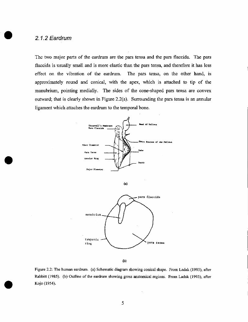
• 2. 1.2 Eardrum

The two major parts of the eardrum are the pars tensa and the pars flaccida. The pars

flaccida is usually small and is more elastic than the pars tensa, and therefore it has less

effect on the vibration of the eardrum. The pars tensa, on the other hand, is

approximately round and conical, with the apex, which is attached to tip of the

manubrium, pointing medially. The sides of the cone-shaped pars tensa are convex

outward; that is clearly shown in Figure 2.2(a). Surrounding the pars tensa is an annular

ligament which attaches the eardrum to the temporal bone.

Sbort Proc... of the Malleua

Dlveh

Armub.r line

Shn1'Oell'. H...br.... "i", r-1Ptu FheoU. ; ,j")

:- \ A'\ Il

Pus Tenu

Major Clameur•(a)

tympanicring

(b)

•Figure 2.2: The human eardrum. (a) Sehematie diagram showing eonieal shape. From Ladak (1993), after

Rabbitt (1985). (b) Outline of the eardrum showing gross anatomieal regions. From Ladak (1993), after

Kojo (1954).

5

•

•

•

The pars tensa is composed of three layers: 1) an outer epidermal layer; 2) the lamina

propria; and 3) an inner mucosal layer. The outer epidermal and inner mucosal are

continuations of the epidermis of the ear canal and the mucous lining of the middle-ear

cavity, respectively. The lamina propria contains a layer ofhighly organized outer radial

fibres and a layer of inner circular fibres. These two layers form the main structural

components of the eardrum.

2. 1.3 Ossieu/ar ehain

An illustration of the human ossicular chain is shown in Figure 2.3. The tip of the

manubrium (umbo) and the lateral process of the malleus are embedded in the eardrum.

The head of the malleus articulates with the body of the incus at the incudomallear joint.

The extremity of the long process of the incus is called the lenticular plate, which forms

the incudostapedial joint with the head of stapes. The head of the stapes continues to the

anterior and posterior crura, which are connected to the footplate.

MALLEUS:

Figure 2.3: The human ossicles. From Ladak (1993), after Anson and Donaldson (1967).

6

•

•

•

There are two muscles in the middle ear, the tensor tympani muscle and the stapedius

muscle. The two muscles acts as antagonist muscles, as a pull of one muscle will result

in a stretching of the other (Karl-Bernd, 1996). Though both muscles help to prevent

transmission of intense vibration to the inner ear, the classical theory of inner-ear

protection by the acoustic reflex has been questioned. According to Prof. Harald

Feldmann (Karl-Bernd, 1996), the muscles may help to maintain the circulation of the

synovial fluid to the joint cartilage by their contraction.

Figure 2.4: The middle-ear muscles.

7

•

•

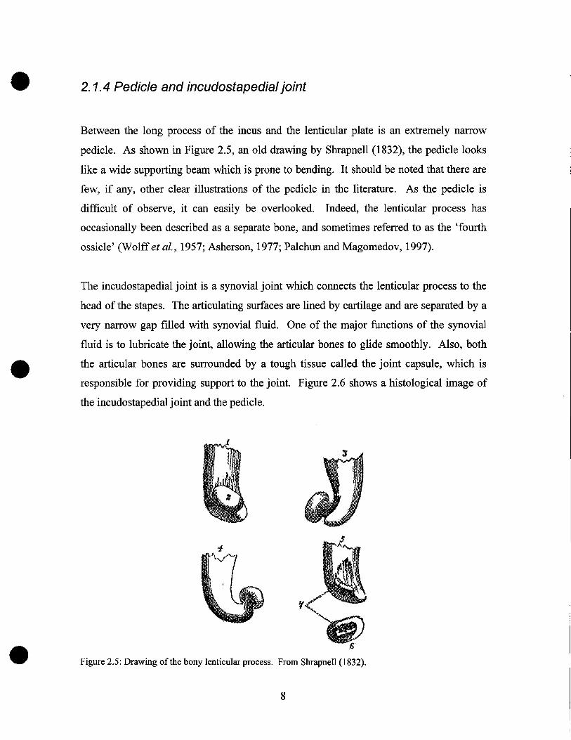
2. 1.4 Pedicle and incudostapedial joint

Between the long process of the incus and the lenticular plate is an extremely narrow

pedicle. As shown in Figure 2.5, an old drawing by Shrapnell (1832), the pedicle looks

like a wide supporting beam which is prone to bending. It should be noted that there are

few, if any, other clear illustrations of the pedicle in the literature. As the pedicle is

difficult of observe, it can easily be overlooked. Indeed, the lenticular process has

occasionally been described as a separate bone, and sometimes referred to as the 'fourth

ossicle' (Wolff et al., 1957; Asherson, 1977; Palchun and Magomedov, 1997).

The incudostapedial joint is a synovial joint which connects the lenticular process to the

head of the stapes. The articulating surfaces are lined by cartilage and are separated by a

very narrow gap filled with synovial fluid. One of the major functions of the synovial

fluid is to lubricate the joint, allowing the articular bones to glide smoothly. AIso, both

the articular bones are surrounded by a tough tissue called the joint capsule, which is

responsible for providing support to the joint. Figure 2.6 shows a histological image of

the incudostapedial joint and the pedicle.

• Figure 2.5: Drawing of the bony lenticular process. From Shrapnell (1832).

8

•

•

•

Figure 2.6: Histological image showing the head of the stapes on the left and the lenticular process on the

right. From Wolff et al. (1957).

2.2 Cat middle ear

The cat middle ear is somewhat similar to the human middle ear. They both have an air

filled cavity which contains a conical eardrum and an ossicular chain, consisting of

malleus, incus and stapes. They do, however, have sorne distinct differences in the

details of the structures. For example, the middle-ear cavity of the cat has a different

configuration, as illustrated in Figure 2.7. The human eardrum is roughly circular while

the cat eardrum is elliptical. The ossicles of the cat and human are shown in Figure 2.8.

9

•

o 5...1·" , r n,,1

Figure 2.7: Middle-ear anatomy ofhuman and cat. After Funnell (1972).

(a)

Cat

(b)

•Figure 2.8: Ossicles of (a) human and (b) cat (right ear, lateral view). From Funnell (1972), (a) after Jayne

(1898), (b) after Nager (1953).

10

•

•

•

Chapter 3

MIDDLE-EAR MECHANICS

3.1 Impedance-matching function

The primary function of the middle ear is to serve as an impedance matcher between the

air-filled outer ear and the liquid-filled inner ear. As the acoustic impedance of the liquid

is higher than that of the air, most of the acoustic energy will be ref1ected if delivered

directly from the air to the liquid. In the auditory system, the presence of the middle ear

helps to increase the sound pressure applied to the inner ear, and hence enhances the

sensitivity of hearing. This increase is obtained by: (a) the ratio of the area of the

eardrum to that of the stapes footplate; (b) the lever ratio of the ossicles; and (c) the

curvature of the eardrum.

The acoustic pressure applied to the eardrum produces a force which is then transferred to

the stapedial footplate. Since the footplate has a smaller surface area than that of the

eardrum, it exerts a greater pressure on the oval window of the inner ear. The increase of

the pressure is roughly equal to the ratio of the two surface areas. For example, if the

effective areas of the eardrum and the footplate are 55 mm2 and 3.2 mm2, respectively,

there will be an approximately 17 times increase of pressure at the footplate. However,

the concept of a fixed area ratio implicitly requires the assumptions that the eardrum

should vibrate as a stiff plate, and that the footplate should act as a piston. As seen from

experimental measurements, neither assumption is true. In fact, the vibration pattern of

the eardrum becomes complex at high frequencies and the displacement of the stapedial

footplate is a combination of piston-like and rocking motions (Khanna and Tonndorf,

1972).

As the manubrium is longer than the long process of the incus, the malleus and incus

have been described as acting as a simple mechanicallever increasing the force applied to

11

•

•

•

the footplate. Assuming a fixed axis of rotation, the increase is equal to the inverse ratio

of the lengths of the lever arms. The length of the incus lever arm is given by the

distance from the axis of rotation to the incudostapedial joint. The eardrum is not

connected only to the umbo, however, but also at other points along the manubrium.

Thus the length of the malleus lever arm should be taken as the distance from the axis of

rotation to a point on the manubrium which represents the centre of action. Similar to the

area ratio, the lever ratio changes with frequency. The change in the lever ratio can be

caused by the shifting of the rotation axis or the flexing of the incudomallear joint at high

frequencies.

The third mechanism of the middle-ear transformer is known as the curved-membrane

effect, originally proposed by Helmholtz (1869). As discussed by Tonndorf and Khanna

(1970), the curvature of the eardrum amplifies the force acting on its surface before it is

applied to the manubrium (Funnell, 1996).

3.2 Eardrum

As stated previously, the vibration pattern of the eardrum becomes complex at high

frequencies, as illustrated in Figure 3.1. For the human eardrum, at frequencies above 2.5

kHz, the vibration pattern breaks up into independently vibrating regions which change

dramatically with frequency (Khanna and Tonndorf, 1972). Similar vibration patterns

have been observed using the finite-element method, which has shown a lot of success in

the modelling of the eardrum since the first finite-element model of it was developed

(Funnell, 1975). Yet, the greatest problem associated with the finite-element modelling is

the lack of accurate measurements on the eardrum's material properties and thickness,

which have a significant effect on the mechanical behaviour.

12

•

•

•

Figure 3.1: Vibration patterns of the cat eardrum measured at (a) 4000 Hz at 117 dB SPL and (b) at

5937 Hz at 114 dB SPL. Atler Khanna, et al. (1996). The vibration pattern changed dramatically when the

frequency was increased from 4 KHz to about 6 KHz; there were more independently vibrating regions at

the higher frequency.

Since the manubrium is coupled to different points on the eardrum, the vibration of the

malleus is therefore affected by the vibrations of different parts of the eardrum (Khanna

and Decraemer, 1996). Certain regions of the eardrum have been found to be 'more

effective in driving the manubrium' (Funnell, 1996). At higher frequencies, the eardrum

is poody coupled to the manubrium (Funnell and Laszlo, 1982).

3.3 Ossicles

The motion of the malleus consists of both rotation and translation, and their magnitudes

may vary with frequency (Decraemer et al., 1991). For the rotational motion, the axis of

13

•

•

•

rotation shifts with frequency (Gundersen, 1972; Gyo et al., 1987) and even within each

cycle (Decraemer et al., 1991). At 10w frequencies, where the rotation component

dominates, the axis of rotation roughly matches the classical fixed rotation axis which

runs from the anterior mallear ligament to the posterior incudal ligament (Guinan and

Peake, 1967).

Guinan and Peake (1967) found that, for sound pressures below 140 to 150 dB SPL

(Sound Pressure Level) and for frequencies less than 3 kHz, the malleus and incus are

rigidly connected by the incudomallear joint. At high frequencies, there is a phase

difference between the malleus and the incus displacements, and that suggests sorne

relative movement within the incudomallear joint.

The other joint in the middle ear is the incudostapedial joint, which has a much smaller

articulating surface. Experimental observations have shown that the joint is non-rigid,

as flexing at the joint has been observed (Guinan and Peake, 1967; Decraemer et al.,

1994). However, the effect of the pedicle was not taken into account in these

observations. As a consequence, it is possible that a portion of the flexibility found

between the incus and the stapes arises from the lenticular process rather than from the

incudostapedial joint. The effect of the pedicle will be discussed later in Chapter 7.

The function of the flexibility of the ossicular joints is still unclear. The middle ear is

always exposed to the external static (or slowly changing) air pressure, which could

induce a huge (up to 1 mm) displacement of the malleus. According to Feldmann

(Hüttenbrink, 1996), the gliding in the ossicular joints is therefore necessary to maintain

small and piston-like displacements at the footplate.

The motion of the stapedial footplate has been studied by different researchers. It is

generally accepted that the motion of the footplate is piston-like, moving in and out of the

oval window (Guinan and Peake, 1967; Dankbaar, 1970; Gundersen and Hogmoen,

1976). Experimental evidence has shown that the amplitude of the footplate

displacement in the z direction (towards the oval window) is ten times greater than that in

14

•

•

•

the x and y directions (in the plane of the footplate). In addition, the stapedial footplate

motion involves complex rocking motions that have much smaIler magnitudes

(Decraemer et al., 2000). According to Gyo et al. (1987), the stapedial footplate rocks

about its longitudinal axis at low frequencies, and the motion of the stapedial footplate

becomes complex at high frequencies. Decraemer et al. (2000) found that aIl 3-D

components of rotation are present in the motion of stapes. At frequencies up to 8 kHz,

the rotation about the long axis of the footplate dominates; and at higher frequencies, the

three components of rotation become comparable.

15

•

•

•

CHAPTER4

THE FINITE-ELEMENT METHOO

4.1 Introduction

The finite-element method is a powerful tool for solving complex structural engineering

problems that involve complicated partial differential equations. The basic principle of

the method is that a continuum (the total structure) is divided into subregions called

elements, which are connected at points called nodes. For each element the behaviour is

described by the element matrices defining the displacements in that region. The

assemblage of all the element matrices forms the equilibrium equations for the

continuum.

The next section will give a brief review of the derivation of the equilibrium equations.

The concept ofmonotonic convergence will be reviewed in Section 4.3; the choice of the

element type will be discussed briefly in Section 4.4.

4.2 General derivation of equilibrium equations

4.2. 1 Overview

The analysis of a system often requires the solution of the differential equations for the

system. It is often very difficult, however, if not impossible, to obtain exact solutions of

the goveming differential equations of the system. This is particularly true if the model

has irregular geometry, for instance. Therefore, approximate solution techniques have

been developed and provide the basis for the finite-element method.

16

• The variational (Rayleigh-Ritz) method and the weighted-residual method are the two

most commonly used techniques (Bathe, 1982). A brief description of the variational

method will be covered in Section 4.2.2.

4.2.2 The variational method

The core of the method involves the principle of stationary potential energy of a system,

II.

where Di represent the degrees offreedom (d.o.f.'s) of the ith node in the system. As dDi

are independent and arbitrary, the only way for dII=O is

•

dIT =t aIl dD; =0;=1 aD;

aIl =0aD;

where i=I,2, .. ,n.

(4.1)

(4.2)

For a linearly elastic body in static equilibrium, the potential energy of the system can be

expressed as

II = (Strain Energy) + (Work Potential Of Extemal Loads)

= U + Q (4.3)

•The strain energy is equal to one-half the integral of strain multiplied by stress, integrated

over the entire volume of the body.

17

• u =! J{.sY {o-}dV2 v

where {s} T is the strain vector and {o-} is the stress vector.

(4.4)

In the constitutive equation, the relationship between stress and strain can be written in

the form

•

{a} = [C]{s}

where [C] is a material matrix. Substituting equation (4.5) into equation (4.4) yields

u =!J{sf[C]{s}dV2 v

The potential of the loads can be expressed as

Q =- Jv{sf {F}dV - Js {S}T {<D}dS - {S}T {Pl

(4.5)

(4.6)

(4.7)

where {F },{ lP } and {P } are the body force vector, the surface traction vector and the

concentrated force vector respectively; and {s } is the displacement vector.

4.2.3 The strain-displacement matrix

Therefore, the total potential energy in one element is

It should be noted that the V and S in (4.8) correspond to the element volume and surface,

• respectively; {s} represents the element nodal displacement vector while {D} is the

18

• structure nodal displacement vector. For convenience in the calculations, it is desirable

to perform the integrals in a local coordinate system. The transformation between the

global and local displacements is given as

{s} = [N]{d} (4.9)

where {s} and {d} are vectors of global and local element displacements, respectively;

[N] is a matrix of displacement interpolation functions. The corresponding element

strains can be expressed as:

{c} = [B]{d} (4.10)

•where [B] is the strain-displacement matrix and can be obtained by differentiating the

element displacement interpolation matrix [N]. Substituting equation (4.10) into the

expression for strain energy (4.6),

•

u =! f {c}T[C]{c}dV =! f {[B]{d} }T[C]{[B]{d} }dV2 v 2 v

=! f {d}T[Bf[C][B]{d}dV2 v

Similarly by using equation (4.9), the potential of the loads can be rewritten as

Q =- fv{sf{F}dV - fs{sf {<I>}dS - {Df {P}

=- fV {d}T {Nf {F}dV - fs {d}T[Nf {<I>}dS - {D}T {P}

19

(4.11)

(4.12)

• 4.2.4 Global finite-element equilibrium equations

Hence the total potential energy in the system, with M elements, is a sum of the potential

energies of all finite elements,

where

[kl = L,,[Bf[CHB]dV

is the element stiffness matrix for element i, and

{rL = fv[Nf{F}dV + L[Nf{<D}dS, ,

(4.13)

(4.14)

(4.15)

• is the element load vector. Equation (4.13) can be rewritten by replacing L{d} by {D},

where

(4.16)

M

[K] =Z)kl andi=1

M

{R}={P}+ ~)rLi=1

(4.17)

Equation (4.16) may be differentiated with respect to each nodal displacement variable in

order to obtain the finite-element equilibrium equations as

•[K]{D} = {R}

20

(4.18)

• Equation (4.18) applies only to the static (or low frequency) case, in which the effect of

inertia and damping are ignored. For a high-frequency dynamic analysis, the finite

element equilibrium equations can be expressed as

[K]{D} + [C]{D}' + [M]{D}" = {R} (4.19)

•

•

where [C] and [M] represent the damping matrix and the mass matrix, respectively;

{Dl' and{D}" are the first and second time derivatives of the displacement matrix,

respectively. Detailed descriptions of equation (4.19) can be .found in many finite

element reference books and will not be covered here.

4.3 Monotonie convergence

The concept of monotonie convergence can be illustrated by Figure 4.1. As shown in the

graph, the dashed monotonie convergence line approaches the exact solution on each

successive mesh refinement. One of the advantages of this behaviour is that a more

precise solution is always guaranteed as the number of finite element increases.

Figure 4.1: Monotonie and non-monotonie convergence. For monotonie convergence, the solution of the

analysis approaches the exact solution D as the number of elements increases.

To ensure monotonie convergence, the e1ements must be complete and compatible. The

completeness of an element means that the displacement function must be able to account

21

•

•

displacements of the element without straining. Constant-strain states indicate that the

strain in each individual element must approach a constant strain as the element size

becomes very small. The compatibility means that the displacements within the elements

and across the element boundaries must be continuous. In another words, no gaps or

overlaps are allowed between elements before or after the analysis.

4.4 Choice of element type

There is a variety of element types that can be employed for finite-element analysis. The

basic element can be as simple as a 2-node line or as complex as a 20-node hexahedral

element. The considerations for the element type normally involve the accuracy of

solution, computer resources required and the geometry of the mode!. In the analysis

presented in this thesis, the tetrahedron has been selected to be the basic three

dimensional element as it could theoretically be used to model any solid structure.

An example of a generalized material matrix [C] for isotropic materials for a three

dimensional element is shown here:

1v v

0 0 0I-v I-v

v1

v0 0 0

I-v I-vv v

1 0 0 0

c= E(1- v) I-v I-v(4.20)

(1 + v)(1- 2v) 0 0 01-2v

0 02(1- v)

0 0 0 01-2v

02(1- v)

0 0 0 0 01-2v

2(1- v)

22

• where E is the material modulus of elasticity (Young's modulus) and v is the Poisson's

ratio.

The finite-e1ement analysis program SAP IV used in the laboratory does not truly support

tetrahedral elements. One possible trick that can be used is to collapse the eight-node

brick e1ement supported by SAP IV to a four-node tetrahedral element, as demonstrated

in Figure 4.2.

z z

y

t

1x

v

5

;--t-----I-Jo- $

1

3 21r--t----__9

4

t

1

1

'f-·---··1

11 r

x•Figure 4.2: Collapsing an eight-node brick element into a tetrahedral element

As mentioned in the Master's thesis of S. Funnell (1989), modifications have to be made

to the code to remove the addition of incompatible modes to the brick element. The

incompatible modes are added to the brick e1ement to reduce the analysis cost and speed

up the convergence rate. The improvement is achieved by adding higher-order

displacement interpolation to represent a constant bending moment. For example,

•23

• 8

U = Lh;u; +a2(1-r2)+a2(1-s2)+a3(1-t2);=18

V = Lh;v; + p2(1-r2)+ P2(1-S2)+ P3(1-t2);=1

8

W = Lh;w; + r2(1- r2) + r2(1- S2) + r3(1-t

2)

;=1

t t

incompatible modes

t

•

•

This is generally advantageous provided the elements are not badly distorted, which is

not the case for the collapsed-brick tetrahedral elements. As a result, the modified code,

written by S. Funnell (1989), is used here for finite-element analysis.

24

• CHAPTER5

MESH GENERATION

5.1 Introduction

Mesh generation is one of the most crucial parts in the finite-element analysis and it is

definitely not a trivial task. Numerous algorithms have been developed and yet mesh

generation is still an ongoing challenge.

Section 5.2 briefly reviews three potential tetrahedral mesh generators: TR4, GRUMMP

and GiD; Section 5.3 compares the three mesh generators in terms of their performance

and capabilities.

• 5.2 Mesh generators

5.2.1 TR4

•

TR4 is a 3-D mesh generator originally developed by Boubez (1986), a Master's student

in the laboratory. The programme was intended to work alongside Fie, a programme

developed locally for segmentation, to construct 3-D biological models. It should be

noted that segmentation is a process of specifying the boundaries of regions of interest

from image sources, such as MRI and histological data. Briefly speaking, the

segmentation programme Fie defines the boundaries of the model and, based on that,

TR4 generates the mesh. The capabilities ofTR4 were further improved by S.M. Funnell

(1989), a Master's student in the laboratory, to handle more general irregularly shaped

objects.

The main philosophy of the algorithm is to construct 3-D meshes between every two

adjacent slices of contours, and assemble aIl the meshes to complete the whole volume

25

•

•

•

mesh. Basically the programme divides the volume between slices into two parts: the

core and the ring, which are dealt with separately. The core is first divided evenly into

triangular prisms and then each prism is divided into six tetrahedra. The mesh generation

for the ring is much more complicated. It should be noted that no additional nodes are

generated during the meshing process, and that is quite different from most of the mesh

generators available. Figure 5.1 shows an example of a 3-D core and ring of two

consecutive 2-D contours.

Sometimes it is possible to reach a situation where the ring cannot he divided into

tetrahedra without modifying its surface triangulation. That, however, would make it

incompatible ta the surface triangulations of the core. The idea of a "flat" tetrahedron is

proposed to preserve the compatibility (see Figure 5.2). The "flat" tetrahedron will be

inflated by relaxation afterward. More detailed descriptions of the TR4 programme can

he found in the Master's theses of Boubez (1986) and Funnell (1989).

Figure 5.1: Core and ring oftwo consecutive 2-D contours. After Funnell (1989)

26

•

•

•

(b)

Figure 5.2: A 'flat' tetrahedron is created in order to preserve compatibility between the surface

triangulations of the core and the ring. After Funnell (1989)

5.2.2 GRUMMP

GRUMMP (Generation and Refinement of Unstructured, Mixed-Element Meshes in

Parallel) is a freely distributed mesh generator. The programme is capable of generating

high-quality 2-D and 3-D meshes. It features sophisticated mesh improvement functions

to reduce poorly shaped elements that can possibly cause numerical problem.

GRUMMP is essentially a Delaunay-based generator. Therefore, the constructed mesh of

tetrahedra has to satisfy the Delaunay criterion that the circumsphere defined by each

tetrahedron contains no mesh nodes in its interior. However, employing the Delaunay

criterion alone is not sufficient to avoid poody shaped tetrahedra. Additionally, it does

not guarantee that the mesh nodes lie within the bounding surfaces. As a result,

additional refinement techniques are usually used to enhance the performance (Yuan and

Fitzsimons, 1993 and Shewchuk, 1998)

27

•

•

In GRUMMP, improvement mechanisms adopted include face swapping and a modified

Laplacian smoothing method (Ollivier-Gooch, 1998). Face swapping is a very common

technique which changes the local connectivity so as to improve the mesh quality. For

example, there are two legal configurations to divide the structure shown in Figure 5.3

into tetrahedra. The objective of the face-swapping algorithm is to select the most

appropriate configuration which minimizes the maximum dihedral angle (angle between

two facets of the tetrahedron) and satisfies the Delaunay criterion. The Laplacian

smoothing method is an operation that optimizes the location of each vertex according to

its neighbours. The smoothing method implemented in GRUMMP is claimed to be

smarter, as it only accepts a change in vertex location if that can lead to improved mesh

quality.

It has been shown that the combination of the swapping followed by the smoothing

technique yields better improvement than applying each mechanism individually (Freitag

and Ollivier-Gooch, 1997). More information about GRUMMP can be found at

http://tetra.mech.ubc.ca/GRUMMPI.

H

•Figure 5.3: Swappable configurations offive points in three dimensions. There are two ways to divide the

structure into tetrahedra. The configuration on the left is preferable and that can be determined by selecting

the one with the smallest maximum dihedral angle. After Freitag and Ollivier-Gooch (1997).

28

•

•

•

5.2.3 GiD@

GiD is a general-purpose pre-postprocessor for finite-e1ement analysis. It adopts the

advancing-front technique, another popular algorithm for mesh generation. Descriptions

of the software can be found at http://gid.cimne.upc.es.

One main problem associated with the traditional De1aunay-based algorithms is that

special care has to be taken to remove elements that lie outside the domain, or cross the

boundary. However, this is not a problem for the advancing-front algorithm. The

method operates by first triangulating the surfaces to create an initial front, and then

moving forward to connect each triangle segment to a fourth node to form a tetrahedron.

The tetrahedron will then be removed and the remaining triangular faces will form the

new fronts. The process will continue until the whole volume is meshed with tetrahedral

e1ements. As the mesh is initiated from the boundary surfaces, the problem of the

elements lying outside the boundary, that may occur in the Delaunay triangulation, is

avoided (George and Seveno, 1994; Moller and Hansbo, 1995).

Figure 5.4: Screen shot ofGiD programme. User is about to start the mesh generation process.

29

•

•

•

5.3 Comparison

Table 5.1 shows a comparison for the three mesh generators. In selecting a suitable mesh

generator, the major consideration is definitely the capability to generate a tetrahedral

mesh on irregularly shaped structures with a high success rate. GiD simply tops the other

two in this category as both TR4 and GRUMMP may occasionally fail in generating the

mesh. In addition, GiD offers the possibility of creating nQn-uniform meshes, which is

helpful in reducing the total number of elements. The programme also comes with a

visualisation tool that has been used extensively in this work to display the finite-element

models and simulation results. A major drawback, however, is that its source code is not

available. In conclusion, GiD has been selected as the best choice among the three.

TR4 GRUMMP GiDSupport Tetrahedral Yes Yes Yes

Element

Control Over Yes Yes Yes

Element size

Support Non-uniform No No Yes

Mesh

Mesh Refinement Smoothing Face swapping, NA.

Laplacian smoothing

Customizable Yes Yes No

Output

Built-in No No Yes

Visualisation Tooi

Friendly No No Yes

Interface

Source Code Yes Yes No

Available

Free Yes Yes No

Technical Support Local Yes Yes

Remarks Fails sometimes Fails sometimes Always works

Table 5.1: Companson ofTR4, GRUMMP and Gill

30

•

•

•

Chapter 6

FINITE-ElEMENT MODEl

6.1 Introduction

This chapter begins with a description of the modelling of the pedic1e and the

incudostapedial joint. The pedic1e-and-joint finite-element model is presented in

Sections 6.2 and 6.3. The pedic1e-and-joint model was tested within an existing model of

the complete middle ear. Section 6.4 gives a brief description of the complete middle-ear

model.

6.2 Pedicle-and-joint modet

6.2. 1 Geometry and dimensions

The pedic1e-and-joint model is a simplified representation of the true anatomy, and

therefore the implementation and the modification, if necessary, of the model can be

accomplished more easily than for a realistic model. The modelling of the simple model

as well as the preliminary simulation results should provide sorne insight into the

development of a more realistic model in the future. Figure 6.1(a) and (b) show

histological images of a cat middle ear. As shown in Figure 6.1(c) and (d), the model

consists of the end of the long process of the incus, the pedic1e, the lenticular plate, the

joint gap, the joint capsule, and the head of the stapes. The dimensions of each structure

were approximated based on histological sections of a cat middle ear. Figure 6.1(e) and

(f) show the model's dimensions that are based on histo1ogica1 sections as shown in

Figure 6.1(a) and (b). Despite the fact that the simple model could easily be meshed with

brick elements, tetrahedral elements are used here because the experience with tetrahedral

elements will help with future work on a more realistic model. Chapter 8 will review the

issue of the realistic model in greater detail.

31

•

•

(a)

(e) side view

(b)

(d) without capsule

(t) top view

•Figure 6.1: (a) is one of the l-I.lm-thick histological seriai sections, stained with toluidene blue, received

2001 Jan from M. McKee (Dept. Anatomy & Cell Biology, McGill University). (b) is one of the 50-1.lffi

thick histological seriaI sections, stained with Hematoxyl and Eosin (H&E), provided by Khanna.

Geometry(c)(d) and dimensions (e)(t) of the pedicle-and-joint model are determined based on histoIogicai

sections (a)(b).

32

•

•

The pedicle is modelled by a 55 !-lm x 160 !-lm x 240 !-lm beam. The joint cavity or gap in

the incudostapedial joint is represented by a 35-!-lm-thick articular cartilage as discussed

in Section 6.2.4. Surrounding the joint is a 30-!-lm-thick layer representing the joint

capsule. To be consistent with the real anatomy of the joint capsule as observed in the

histological sections, only the two ends of the capsule are attached to the bone (see

Figure 6.2).

(a)

Only ends ofcapsule

•

Joint capsule(b)

Figure 6.2: (a) Histology ofjoint capsule (H&E). It should be noted that only the ends of the joint capsule

are attached to the bone, and it has been taken into consideration when building the fmite-element model as

illustrated in (b).

33

•

•

6.2.2 Mechanical Properties

The material properties of the model are assumed to be linear, uniform (i.e., the same in

aH locations) and isotropic (i.e., the same in aH directions). The assumption of linearity is

generaHy valid in the middle ear under normal hearing conditions. At low frequencies at

which the effects of damping and inertia are negligible, the material properties of a linear

isotropic structure can be completely described by its Young' s modulus (Pa or N/m2), and

Poisson's ratio, a dimensionless number.

Poisson's ratio for aH materials has been taken to be 0.3. Explicit sensitivity tests suggest

that varying the Poisson's ratio has little effect on the simulation results of the model,

which matches the earlier findings by FunneH (1975). The tests indicate that mechanical

behaviour of the middle ear is primarily determined by its stiffness and the Poisson's

ratio is found to be less important.

Compact bone

Calcified cartilage

Subchondralbone

(Compact)

•Uncalcified cartilage

Figure 6.3: The nature of lenticular process.

34

•

•

•

As mentioned in the previous chapter, the work presented here has been made possible by

the availability of highly detailed histological sections which show the precise nature of

the pedicle and the incudostapedial joint. With the help of M. McKee, Professor in the

Department of Anatomy & Cell Biology of McGill University, the nature of the material

types has been identified, as illustrated in Figure 6.3.

Calcified cartilage is a cartilage layer close to bone and is about ten times stiffer than

uncalcified cartilage. Most of the lenticular plate is calcified cartilage. The articulating

surface of the lenticular plate is a thin layer of uncalcified cartilage, which stains lighter.

Subchondral bone can be defined as a bone layer just beneath the cartilage, and it serves

as a cushion between the calcified cartilage and the stiffer compact bone. There are

regions of subchondral bone in the lenticular plate. The long process of the incus consists

mainly of compact bone.

The determination of the material properties of living tissues is not easy, because they

can vary widely, depending on their location, direction of measurement, etc. Sections

6.2.3 to 6.2.6 discuss the material properties of the structures in the pedicle-and-joint

mode!.

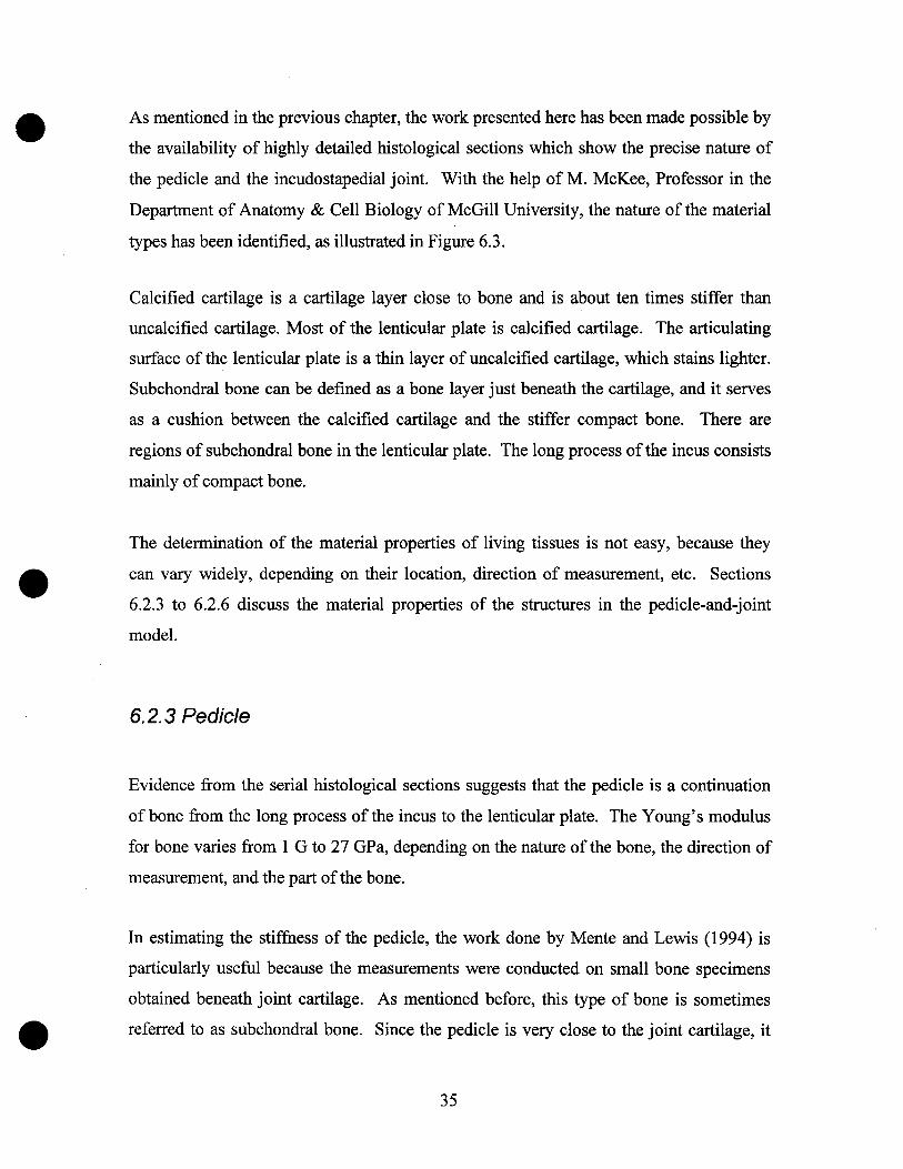
6.2.3 Pedicle

Evidence from the seriaI histological sections suggests that the pedicle is a continuation

ofbone from the long process of the incus to the lenticular plate. The Young's modulus

for bone varies from 1 G to 27 GPa, depending on the nature of the bone, the direction of

measurement, and the part of the bone.

In estimating the stiffness of the pedicle, the work done by Mente and Lewis (1994) is

particularly useful because the measurements were conducted on small bone specimens

obtained beneath joint cartilage. As mentioned before, this type of bone is sometimes

referred to as subchondral bone. Since the pedicle is very close to the joint cartilage, it

35

•

•

•

can be considered as subchondral bone, and therefore a Young's modulus of 5 GPa

(Mente and Lewis, 1994) is adopted for the pedicle.

On the other hand, histological evidence suggests that the pedicle could actually be a

single osteon, the principal organizing feature of compact bone. For a single osteon, the

Young's modulus was calculated to be 10.7 GPa by Ascenzi (1967). A modulus of 21.7

GPa was calculated by Rho et al. (1998), but the value could have been overestimated, as

the bone specimens used were dehydrated, which can lead to an increase in stiffness

(Elices, 2000). Therefore, the simulations also include cases in which a Young's

modulus of 12 GPa is used for the pedicle.

6.2.4 Joint

The incudostapedial joint is a synovial joint, in which the load is transferred from a

cartilage layer on one bone to a cartilage layer on the other bone, either through direct

contact, or through a thin film of synovial fluid between the cartilage layers, or by a

mixture of both. Examination of the histological images shows that the thickness

between the two articulating surfaces is so small that the cartilage on both sides is

probably (at least partially) in direct contact during acoustic vibration. Therefore, the

contacting region in the joint has been modelled as a single block of articular cartilage

(ignoring the synovial fluid space), which has a Young's modulus of around 10 MPa as

measured in normal human articular cartilage (Elices, 2000).

The synovial fluid functions as a lubricant which allows the two articulating surfaces to

glide easily. l t should be noted that the modelling of the thin film of synovial fluid would

be technically complicated. Limited by the finite-element programme SAP IV used in

the laboratory, the sliding contact surface is not implemented in this model. This implies

that the two articulating surfaces in the model are firmly attached and the three

components of the stress are transferred, with no loss, from one surface to another in the

36

•

•

joint. In reality, the stress parallel to the articulating surface will possibly be greatly

attenuated because of the synovial fluid. As a consequence, the in-plane displacements

of the footplate may be smaller than those predicted by the simulation results.

Figure 6.4: Histology showing the incudostapedialjoint. Between the two articulating surfaces is an

extremely narrow gap, filled with synovial fluid (arrow).

6.2.5 Capsule

Another key structure in the model is the incudostapedial joint capsule that completely

encloses the joint. The outer layers of the capsule consist of dense fibrous connective

tissue, the capsule ligament, which dominates the capsule mechanical properties. It is

therefore reasonable to apply the value of Young's modulus for capsule ligament to the

capsule directly. Hewitt and Guilak (2000) reported that the Young's moduli for the hip

joint capsules range from 76.1 ta 285.8 MPa. ltoi et al. (1993) calculated the Young's

modulus for the shoulder joint capsule to be in the range from 31.5±9.4 MPa to 66.9 ±9.4

MPa. In fact, "the overall material behavior properties of the ligaments of different joint

capsules are similar but not identical" (Hewitt and Guilak, 2000).

37

•

•

•

Figure 6.5: Histology showing the joint capsule

Since it is not clear what the Young's modulus of the incudostapedial joint capsule

should be, possible values such as 20 MPa, 50 MPa and 100 MPa are used in the

simulations discussed in the next chapter.

6.2.6 Other structures

The long process of the incus is given a Young's modulus of 12 GPa, corresponding to

stiff compact bone. Since the long process of the incus is so wide that it will bend litlle,

the exact value ofits Young's modulus is unimportant.

The lenticular plate and the head of the stapes consist partly of calcified cartilage and

partly of subchondral bone, and their Young's moduli are 0.3 GPa and 5 GPa,

38

•

•

•

respectively (Mente and Lewis, 1994). Renee an intermediate value of 1 GPa is used as

the Young's modulus for the two structures.

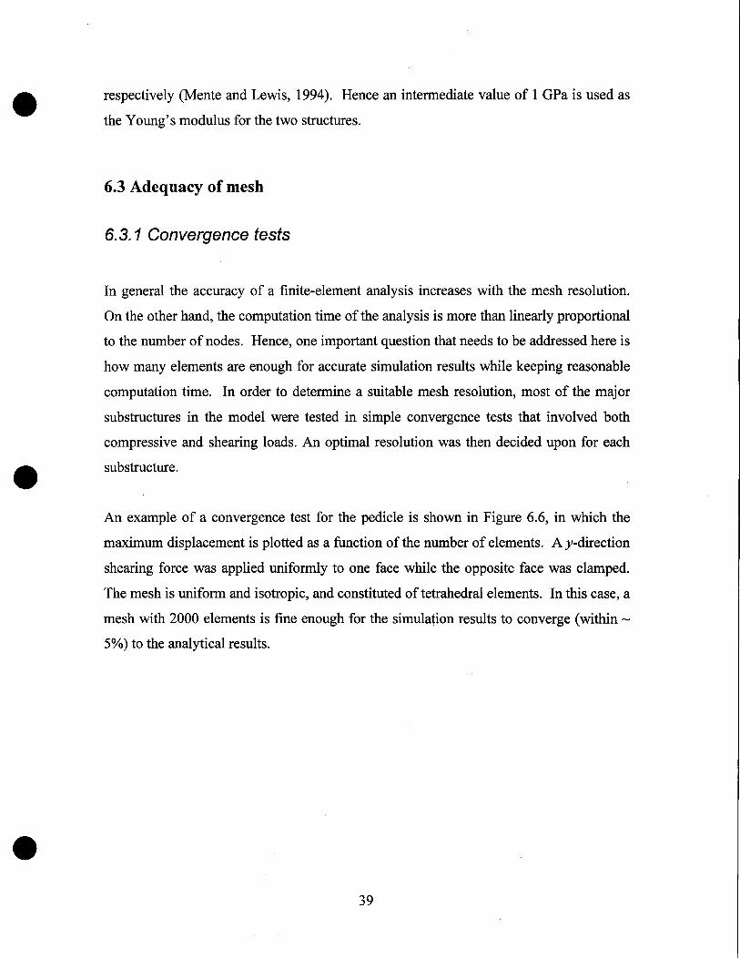
6.3 Adequacy of mesh

6.3. 1 Convergence tests

In general the accuracy of a finite-element analysis increases with the mesh resolution.

On the other hand, the computation time of the analysis is more than linearly proportional

to the number of nodes. Renee, one important question that needs to be addressed here is

how many e1ements are enough for accurate simulation results while keeping reasonable

computation time. In order to determine a suitable mesh resolution, most of the major

substructures in the model were tested in simple convergence tests that involved both

compressive and shearing loads. An optimal resolution was then decided upon for each

substructure.

An example of a convergence test for the pedicle is shown in Figure 6.6, in which the

maximum displacement is plotted as a function of the number of elements. A y-direction

shearing force was applied uniformly to one face while the opposite face was clamped.

The mesh is uniform and isotropie, and constituted of tetrahedral elements. In this case, a

mesh with 2000 e1ements is fine enough for the simulation results to converge (within ~

5%) to the analytical results.

39

300020001000

--""." "',.,.,,~"" ...----//

I-4-SimJIatiOn ReS1.Jtsl"'''--Analylical Results

3,1006-02o

3.200E-02

3,250&02

3400E-02

3,300E-02

•

Figure 6.6: Convergence test for the pedic1e. A y-component shearing load was applied on one face while

the opposite face was c1amped. A mesh resolution with at least 2000 elements is required for high accuracy

in this case.

•Figure 6.7 shows another convergence test for the pedicle; the shearing load was applied

in the x direction in this case. Clearly a mesh with only 2000 e1ements is not even close

to reaching the plateau region of the curve, and a mesh with at least 10000 elements

should be used if the desired discrepancy is less than 5%.

3.500E-Dl .,...------------,

3. ooOE-01 +..:::"":;:".:::",.:::"":;:",.:":"""~""".~,,,,,,~,,,,. -"...-'::".::-...",~"....~.......-"""~".,,..--;._:::---l

5000 10000 15000 20000

No. er.ments

2.500E-Ol ;--....,.~~---------1

2.oo0E-01 +-IJ+/----------I

1.500E-01 +------------11.000&01 -I---------CI.~Si;;:· mJ;;;:latl;ï";·o=n"'i:Rei:su;:::;:lits1

-4-' Ana vtical Re9Jlls 15.000&02 +- -=:==:::i:::ii:::=r.::.;::.::..;..;.:;..::;;:.;.;;;;;...J

0.000800 ;----,...----'T---..----!o

•Figure 6.7: Second convergence test for the pedic1e. An x-component shearing load was applied on one

face while the opposite face was c1amped. A mesh with at least 10000 elements is required for high

accuracy in this case.

40

•

•

6.3.2 Reducing number of e/ements

As illustrated previously, the number of elements required for each substructure can be

determined based on its convergence tests. In the examples presented in the previous

section, where the desirable discrepancy is no more than 5%, the accuracy of the analysis

can always be guaranteed but it cornes at the expense of long computation times.

One way to reduce the computation time is to allow greater discrepancies when deciding

on the number of elements based on the convergence curve. For our present purposes,

discrepancies of up to 30% between the simulation results and the analytical results are

considered to be "acceptable" based on the rationale that the uncertainties of the Young' s

moduli of each substructure are much larger than 30%.

Another way of reducing the number of elements is to use longer and thinner tetrahedral

elements as illustrated in Figure 6.8, in cases where the structure is much larger in one

direction than in another. The quality of the mesh will, however, be affected, as the

tetrahedral elements should ideally be equilateral for the best simulation results. A

poody meshed model is very like1y to cause numerical errors during the solution process

(e.g. Fried, 1972; Babuska and Aziz, 1976). Hence it is important not to over-stretch the

elements. Technically, stretching the elements can be accomplished by applying a

scaling factor to the mesh, in only one direction.

Stretch in one direction

• (a)

41

(b)

'---->

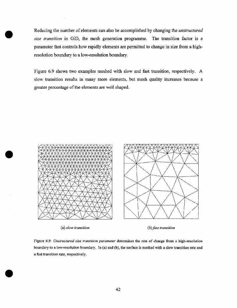
• Reducing the number of elements can also be accomplished by changing the unstructured

size transition in GiD, the mesh generation programme. The transition factor is a

parameter that controls how rapidly elements are permitted to change in size from a high

resolution boundary to a low-resolution boundary.

Figure 6.9 shows two examples meshed with slow and fast transition, respectively. A

slow transition results in many more elements, but mesh quality increases because a

greater percentage of the elements are well shaped.

•

(a) slow transition (b) fast transition

•

Figure 6.9: Unstructured size transition parameter detennines the rate of change from a high-resolution

boundary to a low-resolution boundary. In (a) and (b), the surface is meshed with a slow transition rate and

a fast transition rate, respectively.

42

•

•

•

In GiD, the size transition is represented as a value from 0.0 (slow) to 1.0 (fast). For the

pedicle-and-joint model, a size transition of 0.8 is used to reduce the number of elements.

The scheme that involves stretching of the elements is not adopted because that could

further reduce the quality of the final mesh.

In the final mesh, there are altogether 13209 tetrahedral elements in the model, and each

simulation takes about one hour (PIII 700 MHz, 256 Mbytes RAM) to complete. It

should be noted that the finite-element programme SAP IV fails under Windows on

models with too many elements, as the intermediate file exceeds the 2 GBytes file size

limit of Windows. The file size problem has been solved by running the programme

under Linux.

43

•

•

•

6.4 Middle-ear model

6.4.1 Introduction

To obtain more convincing simulation results from the pedicle-and-joint model, realistic

loading and boundary conditions are required. Obviously, having an applied load in only

one or two directions is not good enough to simulate what really happens in the middle

ear, as the 3-D vibrations of the eardrum, malleus and incus drive the pedicle. Similarly,

having clamped the head of the stapes is a gross simplification of the true situation, in

which the displacements of the stapes are constrained by the annular ligament, stapedial

muscle and cochlear load. As a result, it is desirable to run tests on the pedicle-and-joint

model within a middle-ear model.

Figure 6.10 shows a finite-element model of the cat middle ear which was developed in

this laboratory (Funnell, 1996). The model includes shell representations of the eardrum

and ossicles, and springs representing the middle-ear ligaments and cochlear load. The

model of the eardrum is essentially the same as in previous models (Funnell, 1987, 1992).

The footplate and the cochlear load are equivalent to the models described previously by

Ladak and Funnell (1993, 1994). The incudostapedial joint is represented by a simple

block formed by eight triangular shell elements (Ghosh and Funnell, 1995). Unlike its

predecessors, this model does not have a fixed axis of rotation. Instead, the axis of

rotation is determined by the ligaments, represented by springs, attached to the malleus

and incus (Funnell, 1996).

44

•

•

•

Figure 6.10: Previous fmite-e1ement model of cat middle ear

45

•

•

Details of the existing middle-ear mode1 (Funnell, 1996) will be presented in the

following three sections. The modifications made to it will be discussed in Section 6.4.5.

6.4.2 Eardrum

As shown in Figure 6.8, the eardrum is represented by thin-shell elements. The conical

shape of the eardrum is represented using circular arcs which have one end on the

manubrium and the other along the tympanic ring. The degree of curvature of the arcs,

expressed as a normalized radius of curvature, was set to 1.19 in this model (Funnell and

Laszlo, 1977; Funnell, 1983).

The pars tensa is assigned a Young's modulus of 20 MPa, and a Poisson's ratio of 0.3.

The overall thickness is estimated at 40 Ilm, based on observations by Lim (1968).

6.4.3 Stapedial footplate

The geometry and dimensions of the footplate were determined according to photo

micrographs by Guinan and Peake (1967). The central portion and the rim of the

footplate have thicknesses of 20 Ilm and 200 Ilm, respective1y. Since the footplate is

modelled as compact bone, it is given a Young's modu1us of 20 GPa and a Poisson's

ratio of 0.3.

Attaching the footplate to the oval window is the annular ligament. It constrains the

displacements of the footplate and is represented by in-plane and out-of-plane springs

evenly distributed along the circumference of the footplate (Ladak and Funnell, 1993).

The model of the footplate is shown in Figure 6.11.

46

•

•Figure 6.11: Finite-e1ement model of stapes

The mechanical properties of each spring can be characterized by its stiffness (N/m). For

the out-of-plane springs, which are perpendicular to the plane of the footplate, the total

stiffness is

area2stif.fYzeSStotai =--------

acoustic compliance(6.1)

•

where the acoustic compliance takes into account of the effects of both the annular

ligament and the cochlear load. Given that the acoustic compliance is 0.36 x 10-14 m5/N

(Lynch et al., 1982) and the area of the footplate is 1.26 mm2 (Guninan and Peake, 1967),

the total stiffness is calculated to be 4.4 x 102 N/m (Ladak and Funnell, 1994). Thus, the

stiffness of each spring is equal to the total stiffness divided by the number of springs. In

this mode!, there are 40 out-of-plane springs and therefore each has a stiffness of 11 N/m.

The in-plane displacements of the footplate are constrained by the annular ligament

which determines the stiffness of the in-plane springs. The dimensions of the annular

ligament are considered to be uniform around its perimeter (Guinan and Peake, 1967).

47

• The stiffness of a segment of the annular ligament, which is assumed to have a unifonn

rectangular cross section, is given by:

k= Etl/w (6.2)

•

where E is the Young's modulus, t is the thickness, 1 is the distance between adjacent

nodes and w is the width. With the Young's modulus estimated at 10 kPa (Lynch et al.,

1982) and the dimensions measured from a histological section (Guinan and Peake,

1967), Ladak and Funnell (1996) calculated the stiffness of each segment of annular

ligament, and divided it equally between the springs at the two nodes. In this model, the

in-plane springs are assigned a stiffness of9.9 N/m.

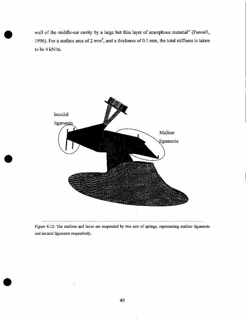
6.4.4 Supporting ligaments

The ligaments which support the ossicular chain are explicitly represented by springs. As

shown in Figure 6.12, there are two sets of springs representing· the ligaments which

attach the middle-ear cavity to the anterior mallear process and the posterior incudal

process, respectively. To be consistent, the stiffness calculated previously by Funnell

(1996) is adopted for the springs. It should be noted that these springs are highly

simplified representations of the ligaments.

Following Funnell's approach (1996), the lateral bundle of the posterior incudalligament

is approximated by a cube with edges of 0.5 mm. Using the previously described

equation k= Etl/w, in which the Young's modulus E is taken to be 20 MPa, Funnell

determined the total stiffness of the ligament to be 10 kN/m. For the medial bundle,

which is about a third as thick, the stiffness is estimated to be 30 kN/m.

Similarly, three spring elements are used to model the elastic suspension of the malleus.

In fact, it is a very crude representation because "the malleus appears to be attached to the

48

• wall of the middle-ear cavity by a large but thin layer of amorphous material" (Funnell,

1996). For a surface area of2 mm2, and a thickness of 0.1 mm, the total stiffness is taken

to be 4 kN/m.

•

Incudal

Mallear

•

Figure 6.12: The malleus and ineus are suspended by two sets of springs, representing mallear ligaments

and ineuda1ligaments respeetively.

49

•

•

•

6.4.5 Modifications

At the time the original middle-ear model was constructed, the high-resolution histology

and MRI data were not yet available. Problems were found when comparing the original

model with the most recent 3-D reconstructions from histology and MRI. Renee, sorne

modifications were made to the original model, in particular to the alignment of the

footplate and to the location of the elastic suspensions of the malleus and incus.

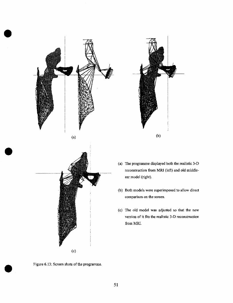
A new programme was developed to offer a friendly environment to display and

manipulate the finite-element models. The programme was implemented with OpenGL

in C. As illustrated in Figure 6.13, the basic principle of the programme is to allow the

user to superimpose two models and adjust the old model to fit the realistic 3-D

reconstructions from histology or MRI.

The programme displays the 3-D reconstruction and the finite-element model

simu1taneously, allowing direct comparison by inspection on the screen. Using the

eardrum as reference, two models are superimposed as the first step. The user then

selects parts, i.e. the stapes, which require changes. The user can translate and rotate the

selected parts of the old model in the x, y and z directions. The programme also provides

features such as zoom, change ofviewing angles, change of the degree of rotation, etc.

50

•

•

•

(a)

(c)

Figure 6.13: Screen shots of the programme.

(b)

(a) The programme displayed both the realistic 3-D

reconstruction from MRI (left) and old middle

ear model (right).

(b) Both models were superimposed to allow direct

comparison on the screen.

(c) The old model was adjusted so that the new

version of it fits the realistic 3-D reconstruction

fromMRI.

51

•

•

•

Figure 6.14(a) and (b) show the 3-D reconstruction from MRI and the modified finite

element model of the middle ear, respectively. The bold line shown in the figure is the

supposed axis of rotation, corresponding to the classical concept of a fixed axis through

the anterior process of the malleus and the posterior process of the incus. The fixed axis

of rotation is roughly parallel to the long axis of the footplate. Illustrations of the models

from different perspectives are shown in Figure 6.15.

(a)

(b)

Figure 6.14: (a) 3-D reconstruction from MRI. (b) Finite-element model of middle ear. The solid bold

lines correspond to the classical axis of rotation, running from the anterior mallear tip to the posterior

incudal tip. The dashed lines correspond to the long axis of the footplate.

52

•

• (a)

(b)

•Figure 6.15: 3-D reconstruction from MRI and fmite-element model of middle ear viewed from different

perspectives.

53

• The pedicle-and-joint model has been incorporated into the middle-ear model

(Figure 6.16). Careful attention has been paid to the pedicle-and-joint model's

alignment, which is determined based on the 3-D reconstruction from the histological

data of the middle ear. The complete model of the middle ear is shown in Figure 6.17.

•

~,.,.--- ... ,...",

\\

\.\

\ ..

•

Figure 6.16: The pedicle-and-joint model is incorporated in the middle-ear model, replacing the old

tepresentation of the incudostapedialjoint.

54

•

• (a)

Figure 6.17: (a) Finite-element model ofmiddle ear after including the pedicle-and-joint mode!.

(b)(c) Pedicle-and-joint model within the middle-ear model from different perspectives.•(b) (c)

55

•

•

6.5 Bandwidth minimization

The computation time can be greatly reduced if the nodes of the mesh are numbered in a

specifie order that minimizes the bandwidth, the width of the band of non-zero numbers

which lies along the diagonal of the stiffness matrix. For the models presented here, the

minimization of the bandwidth is performed, using a bandwidth-minimization

programme written by Funnell, based on the algorithm of Crane et al (1976).

6.6 Input stimulus

For the isolated pedicle-and-joint mode!, the exact input is not known but it can be

simulated with small loads for the purposes of this study. A uniform static pressure was

applied on the long process of the incus; one surface of the head of the stapes was

clamped (Figure 6.18). The simulation results for this model will be discussed in

Section 7.1.

Uniform pressure !CI mped

•Figure 6.18: A unifonn pressure was applied the pedicle-and-joint model. One surface of the head of the

stapes was clamped.

56

•

•

•

For the middle-ear mode!, a uniform sound pressure of 100 dB SPL, equivalent to 2.828

Pa, is applied to the eardrum. Since the middle ear behaves linearly up to 130 dB SPL

(Guinan and Peake, 1967), the assumption of linearity in this model is not violated. The

frequency of the input is taken to be low enough so that the damping and inertial effects

can be ignored.

57

•7.1 Pedicle-and-joint model


Chapter 7

RESULTS

Section 7.1 presents the simulation results of the isolated pedicle-and-joint mode!. As

discussed in the preceding sections, the mechanical properties of the middle-ear

structures are uncertain and therefore the tests are designed explore variations in the

Young's moduli of various substructures in the pedicle-and-joint mode!. Section 7.1.2

shows the results for the base case in which a set of plausible estimates of the Young's

moduli, as discussed in Chapter 6, is adopted. The results after varying the Young's

moduli of the pedicle and the joint are presented in Section 7.1.3 and 7.104, respectively.

• A summary of the results of the isolated pedicle-and-joint model is presented in Section

7.1.5.

As the displacements of the ossicles are on the order of nm (10-9 m), the simulated

deformations presented here were scaled up so that the displacements can be seen.

•58

•

•

7. 1.2 Base case

Figure 7.1 shows the simulation results for the isolated pedicle-and-joint mode! in which

the Young's moduli of its substructures are as given (refer to Sections 6.2.2 to 6.2.6) in

Table 7.1.

Pedicle: 5 GPa;joint gap: 10 MPa; capsule: 50 MPa

Figure 7.1: The simulation results for the base case. The deformations were scaled up so that the

displacements, on the order of nID, can be seen.

Long process of incus

Pedicle

Lenticular plate

Joint gap

Head of stapes

Joint capsule

Young's modulus (Pa)

•Table 7.1: The Young's moduli of the substructures in the pedicle-and-joint model in the base case.

59

•

•

•

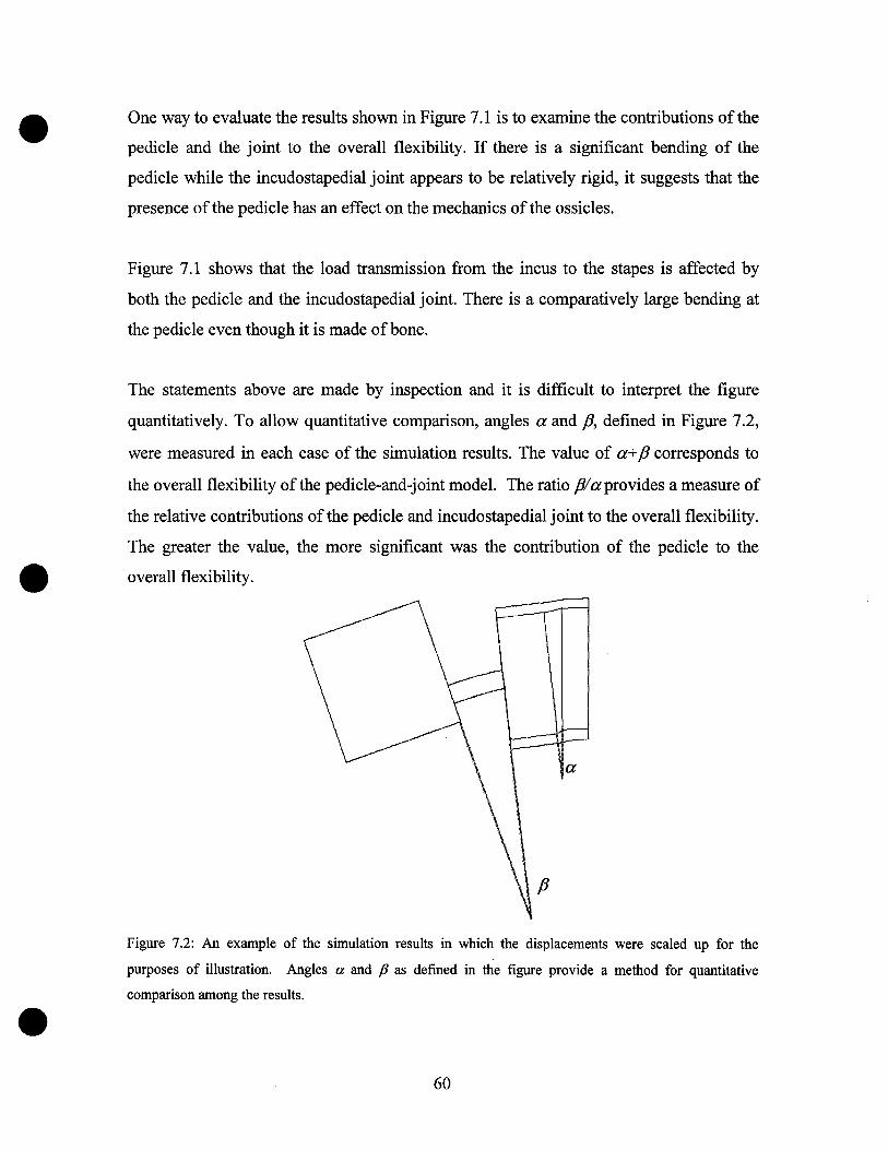
One way to evaluate the results shown in Figure 7.1 is to examine the contributions of the

pedicle and the joint to the overall flexibility. If there is a significant bending of the

pedicle while the incudostapedial joint appears to be relatively rigid, it suggests that the

presence of the pedicle has an effect on the mechanics of the ossicles.

Figure 7.1 shows that the load transmission from the incus to the stapes is affected by

both the pedicle and the incudostapedial joint. There is a comparatively large bending at

the pedicle even though it is made ofbone.

The statements above are made by inspection and it is difficult to interpret the figure

quantitatively. To allow quantitative comparison, angles a and fi, defined in Figure 7.2,

were measured in each case of the simulation results. The value of a+fi corresponds to

the overall flexibility of the pedicle-and-joint mode!. The ratio fi/aprovides a measure of

the relative contributions of the pedicle and incudostapedial joint to the overall flexibility.

The greater the value, the more significant was the contribution of the pedicle to the

overall flexibility.

a

fi

Figure 7.2: An example of the simulation results in which the displacements were scaled up for the

purposes of illustration. Angles a and j3 as defmed in the figure provide a method for quantitative

comparison among the results.

60

•

•

There are different methods for calculating the angles a and /3, and the following

example demonstrates the method used in this thesis.

Figure 7.3: An illustration showing how the angle fi is calculated.

As illustrated in Figure 7.3, the angle /3is given by

•

/3 = /31 - /32Ale-Ale Ale-Ale=sin-I 1 2 _ sin-I 3 4

II 12

Since the angles /31 and /32 are very small, equation 7.1 can be rewritten as

/3 ~ Alel - Ale2 _ Ale3 - Ale4

II 12

61

(7.1)

(7.2)

• For the base case, the values of the angles a, fJ, a+fJ and the ratio fJla are listed in Table

7.2. In this case, the bending at the pedicle is significant since the angle fJ is about seven

times greater than a

a

(~rad)

p(~rad)

a+p

(~rad)

pla

p:5 G; j: 10 M; c:50 M

(Base case)

•

•

Table 7.2: Angles a, f3, a+f3 and the ratio f3la for the base case. The Young's moduli (measured in Pa) of

the pedicle, joint gap and capsule are represented by p,j and c, respectively.

7. 1.3 Variation ofjoint stiffness

The Young's moduli of the joint gap and capsule were varied as discussed in Chapter 6.

The simulation results are shown in Figure 7.4. The values of the angles a, fJ, a+fJ and

the ratio fJla for these cases listed in Table 7.3. For these cases, the pedicle bending (f3) is

almost constant at Il.8.

In Figure 7.4 (a), the flexibility of the joint increases since the Young's modulus of the

joint gap is reduced from 10 MPa to 5 MPa. The value of a increases by 40% as the

stiffness of the joint gap decreases by 50%.

In Figure 7.4 (b) and (c), the Young's modulus of the joint capsule was reduced from

50 MPa to 20 MPa, and increased to 100 MPa, respectively. For case (b), the 60%

decrease of the capsule stiffness leads to a 66% increase of angle a For case (c), the

doubling of the capsule stiffness results in a 42% decrease of the angle a

In Figure 7.4 (d), the Young's moduli of the joint gap and the capsule were both reduced,

to values of 5 MPa and 20 MPa, respectively. The value of a increases by 170%. The

62

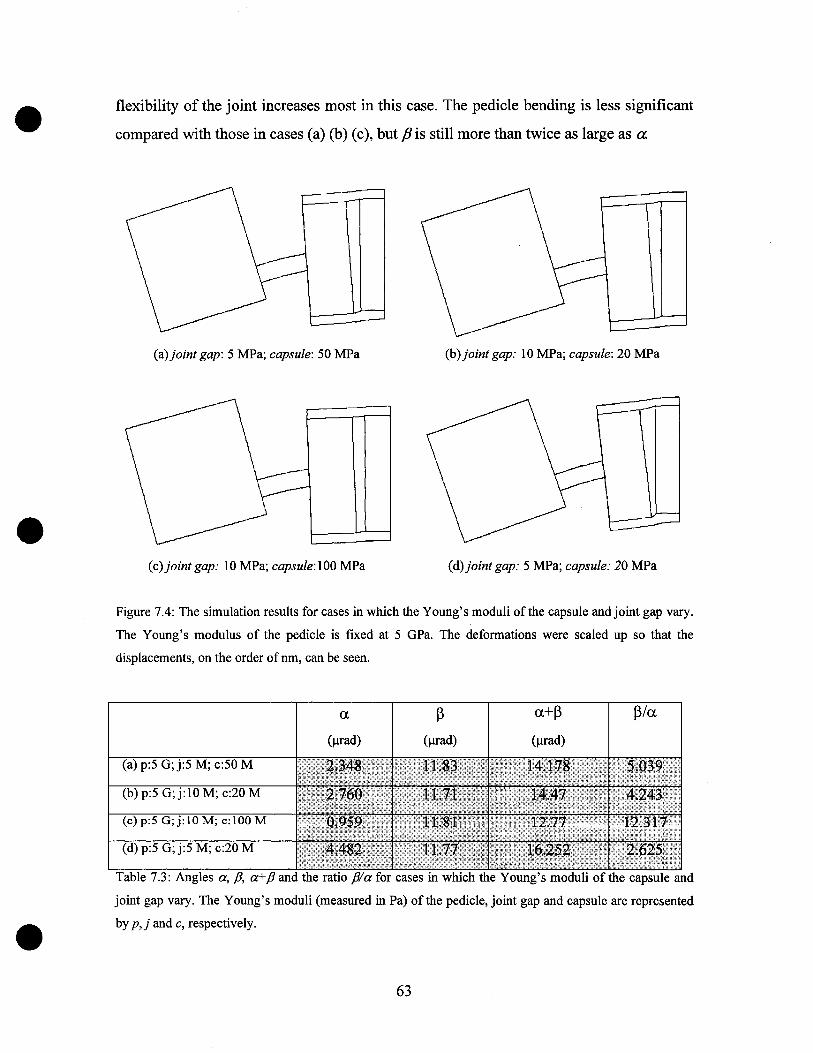
• flexibility of the joint increases most in this case. The pedicle bending is less significant

compared with those in cases (a) (b) (c), but fJ is still more than twice as large as a

•

(a)joint gap: 5 MPa; capsule: 50 MPa

(c) joint gap: 10 MPa; capsule: 100 MPa

(b)joint gap: 10 MPa; capsule: 20 MPa

(d)joint gap: 5 MPa; capsule: 20 MPa

Figure 7.4: The simulation results for cases in which the Young's moduli of the capsule and joint gap vary.

The Young's modulus of the pedicle is ftxed at 5 GPa. The deformations were scaled up so that the

displacements, on the order of nm, can be seen.

Table 7.3: Angles a, P, a+p and the ratio pla for cases in which the Young's moduli of the capsule and

joint gap vary. The Young's moduli (measured in Pa) of the pedicle, joint gap and capsule are represented

by p,j and c, respectively.•

(a) p:5 G;j:5 M; c:50 M

(b) p:5 G;j:l0 M; c:20 M

(c) p:5 G;j:IO M; c:IOO M

(d) p:5 G;j:5 M; c:20 M

a a+~

(Jlrad)

~/a

63

•

•

7. 1.4 Variation of pedicle stiffness

Figure 7.5 shows the simulation results where the Young' s modulus of pedic1e varies as

discussed in Chapter 6. The values of the angles a, /3, a+/3 and the ratio /3/a for these

cases are listed in Table 7.4.

In Figure 7.5 (a) the pedic1e stiffness was increased from 5 GPa to 12 GPa, to equal that

of the long process of the incus. As the pedic1e becomes stiffer, the degree of the pedic1e

bending decreases by 35% but it is still about 4.5 times as large as that ofthe joint.

In Figure 7.5 (b) the Young's modulus of the pedic1e was reduced from 5 GPa to 3 GPa.

In contrast to case (a), the degree of the pedic1e bending increases by 39% and this case

results in a significant increase of the ratio /3/a It also has the highest value of a+f3,

indicating the greatest flexibility of the pedic1e-and-joint model.

(a) Pedicle: 12 GPa (b) Pedicle: 3 GPa

•

Figure 7.5: The simulation results for cases in which the Young's modulus of the pedicle varies. The

deformations were scaled up so that the displacements, on the order of nm, can be seen. The Young's

moduli of the joint gap and capsule are fixed at value of 10 MPa and 50 MPa, respectively.

64

• a

(~ad)

~

(~rad)

a+p

(~rad)

pla

(a)p=12 G;j=IO M; c=50 M

(b)p=3 G;j=lO M; c=SO M

•

•

Table 7.4: Angles a, /3, a+/3 and the ratio fJ/a for cases in which the Young's modulus of the pedicle

varies. The Young's moduli (measured in Pa) of the pedicle, joint gap and capsule are represented by p,j

and c, respectively.

7. 1.5 Summary

In general, the bending at the pedicle is more significant than the flexing at the

incudostapedial joint since the ratios fJ/a are always greater than 2.5 for these parameters.

Relative contributions to the overall bending vary as expected as the parameters are

varied.

The change of the moduli of the joint and capsule has little effect on the bending at the

pedicle. Conversely, the change of the modulus of the pedicle has little effect on the

bending of the joint and capsule. The flexibility of the joint increases most when the

Young's moduli of the joint and the capsule are both reduced; their respective

contributions to the increased flexibility are roughly the same. The pedicle bends most

when its stiffness is reduced: decreasing its Young's modulus by 40% increases f3 by

about the same percentage.

65

• 7.2 Middle-ear model


As stated in Section 6.4, the loading and boundary conditions in the isolated pedicle-and

joint model are highly simplified. As a result, the pedicle-and-joint model has been

included in the middle-ear model for more sophisticated investigation (Figure 6.16).

The middle-ear model is suspended by springs representing the suspending ligaments and

cochlear loads. A uniform sound pressure of 100 dB SPL is applied to the eardrum. Once

again, a range of plausible values is used for the Young's moduli for the pedicle, joint

and capsule.

7.2.2 Validation of the middle-ear model•7.2.2.1 Static displacements of the eardrum

Figure 7.6 shows the low-frequency vibration pattern of the eardrum in the middle-ear

model. The maximum eardrum displacement and the umbo displacement can be used to

characterize the eardrum and manubrium movements. For the midd1e-ear model

presented here, the maximum eardrum disp1acement (308 nm) is about 2.3 times as large

as the umbo displacement (135 nm). The vibration pattern and the magnitudes of the

maximum displacements are similar even when the stiffness of the pedicle-and-joint part

of the model changes. The results are similar to the results obtained in earlier models

developed by Ghosh (1996) and Funnell (1996). For those two earlier models, the

maximum eardrum displacement and the umbo displacement are 232 nm and 74 nm, and

258 nm and 105 nm, respectively.

•66

•

•

•

Figure 7.6: Vibration pattern of the eardrum. The maximal displacements of the eardrum and

manubrium are 308 and 135, respectively.

67

• 7.2.2.2 Footplate displacements

The displacement of the central node is used here to represent the displacement of the

footplate. For the middle-ear model presented here, the footplate displacements in the x,

y and z directions are 3.71 mn/Pa, 4.17 nmlPa and 11.3 nmlPa, respectively. The footplate

displacement in the z direction is, as expected, greater than that in the other directions.

The magnitude of the z displacement is, however, only about one third of the values of

the experimental measurement (Guinan and Peake, 1967; Decraemer et al., 2000).

Table 7.5 lists the values of the maximum eardrum displacement, umbo displacement

(maximum manubrium displacement), and footplate displacement in the z direction, as

reported by different 'authors.

•x

~z

•

Figure 7.7: Finite-element model of the footplate.

68

• Maximum

disp1acement of Disp1acement of the

the eardrum umbo

z disp1acement of

the footp1ate

•

•

Ghosh (1996) *Funnell (1996)

Mode1 presented here

Guinan & Peake (1967)

Decraemer et al. (2000)

ootplate

displacement in the z direction, reported by different authors. The frequency of the input stimulus is below

lOO Hz. The displacements are normalized to a stimulus of 1 Pa.

* Finite-element model has a fixed rotation axis

The finite-e1ement mode1s ofmidd1e ear listed in Table 7.5 include the midd1e-ear mode1

presented in this thesis, and the mode1s deve10ped by Ghosh (1996) and Funnell (1996).

The midd1e-ear mode1 constructed by Ghosh (1996) is the earliest among the three, and it

has a fixed rotation axis. An improved version of that mode1 was constructed by Funnell

in 1996. For the improved mode1, the rotation axis is determined by the suspending

ligaments, and the representations of the ossicles are greatly improved. For the middle

ear model presented here, the alignment problem in its predecessors has been corrected.

In addition, a pedicle-and-joint representation is included in the model.

Although the three middle-ear models are closely related, there are clear differences,

especially in the representation of the ossicles. That may explain the differences in the

maximum eardrum displacement and the umbo displacement among the three mode1s, as

shown in Table 7.5. For the three middle-ear models, the ratio between the maximum

eardrum disp1acement and the umbo displacement is nevertheless roughly the same.

69

•

•

•

In the model constructed by Ghosh (1996), the distance between the stapes and the plane

of the tympanic ring is about three times greater than that in the anatomy, and that results

in a much greater lever ratio of the ossicles. That explains the large z component of the

footplate displacement which is about three times greater than that of the other two

models listed in Table 7.5.

The discrepancy of the z component of the footplate displacement between the simulation

results and the experimental measurements could come from many sources in the middle

ear model: uncertainties of the Young's moduli, highly simplified representation of the

supporting ligaments, insufficiency of finite elements in the mesh, etc.

To examine the effect of the supporting-ligament alignment on the z component of the

footplate displacement, 15 test cases were designed having different alignments for the

springs representing the ligaments. In one trial, the z displacement of the footplate could

be increased by -20%. A simulation was also done with a fixed axis of rotation, in case

the flexibility of the supporting springs was responsible for the decreased footplate

displacement, but this did not seem to be the case. The hours of simulation time

discourage any further effort to tune up the displacement just by trial and error.

70

•

•

•

7.2.2.3 Axis of rotation

Figure 7.8 shows the medial view of the displacement-amplitude contours of the model.

The contour with zero displacement indicates the position of the axis of rotation. As

expected, the axis of rotation is roughly parallel to the classical fixed axis, running from

the anterior mallear tip to the posterior incudal tip.

rotation

Figure 7.8: Visualisation of the displacement pattern for the displacement component along the axis normal

to the plane of the page. The axis of rotation for this model is roughly parallel to the classical axis of

rotation.

71

•

•

•

7.2.3 Pedicle-and-joint model

The simulation results for the pedicle-and-joint part of the middle-ear model will be

evaluated in the same manner as described in Section 7.1. Figure 7.9 shows the results

for the base case; Figure 7.10 and 7.11 show the results after varying the stiffness of the

joint and pedicle, respectively. The deformations are scaled up so that the displacements,

on the order of nm, can be seen.

Table 7.6 lists the measurements of a, p, a+p and the ratio pla in these seven different

cases.

Pedicle: 5 GPa;joint gap: 10 MPa; capsule: 50 MPa

Figure 7.9: The simulation results for the pedicle-and-joint part in the middle-ear model for the base case.

72

•

•(a)joint gap: 5 MPa; capsule: 50 MPa

(c)joint gap: 10 MPa; capsule: 100 MPa

(b)joint gap: 10 MPa; capsule: 20 MPa

(d)joint gap: 5 MPa; capsule: 20 MPa

•

Figure 7.10: The simulation results for the pedicle-and-joint part in the middle-ear model, for cases in

which the Young's moduli of the capsule and joint gap vary. The Young's modulus ofthe pedicle is fixed

at 5 GPa.

73

•

(a) Pedicle: 12 GPa (b) Pedicle: 3 GPa

•

Figure 7.11: The simulation results for the pedicle-and-joint part in the middle-ear model, for cases in

which the Young's modulus of the pedicle varies. The Young's moduli of the joint gap and capsule are

fixed at value of 10 MPa and 50 MPa, respectively.

Pedicle-and-joint part in middle-ear model

a

(prad)

~

(prad)

a+~

(prad)

~/a

(a) p=5 G;j=IO M; c=50 M

Base Case

(b)p=5 G;j=5 M; c=50 M

(c) p=5 G;j=10 M; c=20 M

(d)p=5 G;j=lO M; c=100 M

(e)p=5 G;j=5 M; c=20 M

(f)p=12 G;j=IO M; c=50 M

(g)p=3 G;j=10 M; c=50 M

•Table 7.6: Angles a, p, a+p and the ratio pla for the seven different cases shown in Figure 7.9, 7.10 and

7.11. The Young's moduli (measured in Pa) of the pedicle,joint gap and capsule are represented by p,j

and c, respectively.

74

•

•

The simulation results are consistent with those obtained when the pedicle-and-joint

model was tested alone. The results suggest that most of the flexibility between the incus

and the stapes actually originates from the pedicle rather than from the incudostapedial

joint.

Table 7.7 summarizes the measurements of a, p, a+p and the ratio pla for the isolated

pedicle-and-joint model. Tables 7.6 and 7.7 both indicate that reducing the stiffness of the

pedicle results in the greatest values of fi a+p and pla. The value of ~ a measure of the

joint flexibility, increases most when the Young's moduli of the joint and the capsule are

both reduced. In contrast, the flexibility of the joint decreases drastically when the

Young' s modulus of the joint capsule is increased to 100 MPa.

There is a twisting at the pedicle-and-joint model within the middle-ear model. The

presence of the twisting is not very surprising since the motion of the ossicles is

complicated. Indeed, the twisting may correspond to the in-plane rotation of the footplate

as discussed in Chapter 3.

Isolated pedicle-and-joint model

Table 7.7: Angles a, p, a+p and the ratio pla for the isolated pedicle-and-joint model. The Young's

moduli (measured in Pa) of the pedicle, joint and capsule are represented by p,j and c, respectively.•

(b) p=5 G;j=10 M; c=50 M

Base Case

(b)p=5 G;j=5 M; c=50 M

(c) p=5 G;j=10 M; c=20 M

(d)p=5 G;j=10 M; c=100 M

(e) p=5 G;j=5 M; c=20 M

(t) p=12 G;j=lO M; c=so M

(g) p=3 G;j=lO M; c=50 M

a.

(Ilrad)

a.+p

(Ilrad)

pla.

75

•

•

•

In the results shown in Figures 7.9 to 7.11, there are "ears" at the corners of the stapes

head. It should be noted that for simplicity the crura have been attached only to the four

corners (nodes) of the stapes head of the pedic1e-and-joint model. The stresses from the

stapes head are transferred to the crura on1y via four nodes, and therefore these four

nodes have greater displacements compared with other nodes on the stapes-head surface.

These "ears" indicate that part of the energy transferred from the stapes head to the crura

has been dissipated, and that could affect the accuracy of the simulation results. One way

to solve the problem is to use more nodes to attach the stapes head to the crura.

Figure 7.12 shows a c1ose-up view of the "ears".

Joint Capsule

Figure 7.12: Close-up view ofthe "ears".

76

•

•

•

Chapter 8

CONCLUSION AND FUTURE WORK

8.1 Conclusion

This is the first attempt to model the pedicle and the incudostapedial joint in such detail.

A great deal of effort was devoted to the mesh generation and material properties of the

model. The pedicle-and-joint mode1 was tested in two different ways. On the one hand,

the mode1 was tested in isolation; on the other hand, the model was tested within an

existing middle-ear model. The mode1 was subjected to a low-frequency load, where the

effects of inertia and damping are negligible.

The pedicle-and-joint model consists of the end of the long process of the incus, the

pedicle, the lenticular plate, the joint gap, the joint capsule, and the head of the stapes.

The shape and dimensions of the model were based on histological sections of a cat

middle ear. Special attention has been paid to the material properties of the structures in

the models. Possible values for the Young's moduli of the joint,joint capsule and pedicle

were examined.

The pedicle-and-joint model was constructed using tetrahedral elements. Convergence

tests were conducted to determine the number of e1ements required for each substructure

in the model. The issue of the compromise between the mesh resolution and the

computation time was investigated.

An existing finite-element mode1 of the cat middle ear was modified to include the new

pedicle-and-joint component. Sorne alignment problems of the old model were found

when comparing it with the most recent 3-D reconstructions from histology and MRI. To

solve the problems, a programme was deve10ped to offer a friendly environment to

display and manipulate the finite-element models.

77

•

•

The simulation results of the middle-ear model are consistent with those of the simple

pedicle-and-joint model. The results suggest that the bending at the pedicle is more

significant than the flexing at the incudostapedial joint. In other words, most of the

flexibility between the incus and the stapes actually originates from the bony pedicle

rather than from the incudostapedial joint itself.

8.2 Future Work

The next phase of the project will be to use more realistic models which are constructed

based on histology and/or MRI. For example, the modelling of the form of the pedicle

should be improved. In fact, as shown in Figure 8.1, more realistic surface models of the

pedicle and the middle ear have recently been developed in the laboratory. In addition,

the estimates of the parameters used in the model, such as the Young's moduli, should

ideally be refined using data derived from experimental studies on the middle ear itself

rather than the existing measurements on other parts of the body.

Figure 8.1: More realistic models of (a) lenticular process and (b) cat middle ear. Both models were

constructed by Funnell.•(a) (b)

78

•

•

•

Long computation time is one of the main problems for the model presented here, and

will get even more serious for more realistic models, which often involve a tremendous

number of nodes. As a result, there must be some new algorithms, or more powerful

hardware, to reduce the computation time to a comfortable level.

In order to have a better representation of the joint, the finite-element programme should

be able to model the gliding contact surface and the synovial fluid. In fact, this feature

has already been included in many recent finite-element programmes.

For the simulation results presented in this thesis, the frequency of the input stimulus is

assumed to be low enough so that the effects of the inertia and damping can be ignored. It

would be useful to extend the frequency range. The main challenge here is to estimate

the damping coefficients. In addition, the computation time would increase drastically

compared with that in a static test. Some work is needed to reduce the simulation time.

79

•

•

•

REFERENCES

Ascenzi A, Bonucci E (1967): "The tensile properties of single osteons" Anat Rec. Aug 158(4),

375-86

Babuska l, Aziz AK (1976): "On the angle condition in the finite element method" SIAM J.

Numer. Anal. 13,214-226

Bathe KJ (1982): "Finite element procedures in engineering analysis" Prentice-Hall, New Jersey

Békésy GV (1941): "On the measurement of the amplitude of vibration of the ossicles with a

capacitive probe" Akust. Zeitschr, Vol.6, 1-16 [in German]

Boubez TI (1986): "Three-dimensional finite-element mesh generation using seriaI sections"

M.Eng. Thesis, McGill University, Montréal.

Crane Jr. HL, Gibbs NE, Poole Jr. WG, Stockmeyer PK (1976): "Algorithm 508. Matrix

bandwidth and profile reduction" ACM Trans. Math. Software 2, 375-377, Complete source in

"Collected Algorithms" from ACM

Dankbaar WA (1970): "The pattern ofstapedial vibration" J. Acoust. Soc. Am., 48,1021-22

Decraemer WF, Khanna SM, Funnell WRJ (1991): "Malleus vibration mode changes with

frequency" Hearing research, 54, 305-318

Decraemer WF, Khanna SM, Funnell WRJ (1994): "A method for determining three dimensional

vibration in the ear" Hear. Res., 77, 19-37.

Decraemer WF, Khanna, SM, Funnell WRJ (2000): "Measurement and modelling of the three

dimensional vibration of the stapes in caf' Proc. Internat. Symp. on Recent Developments in

Auditory Mechanics (Sendai, Japan, 1999 July), World Scientific Pub., US, UK, Singapore, 36

43

80

•

•

•

Elices M (2000), "Structural Biological Materials". Pergamon, Amsterdam, xv+361 pp.

Fried 1 (1972): "Condition offinite element matrices generated from nonuniform meshes", AIAA

Journal 10, pp.219-221

Freitag LA, Ollivier-'Gooch (1997): "Tetrahedral mesh improvement using swapping and

smoothing" International Journal for Numerical Methods in Engineering, v 40,3979-4002

Funnell SM (1989): "An approach to finite-element modeling of the middle-ear" M.Eng. Thesis,

McGill University, Montréal

Funnell WRJ (1972): "The acoustical impedance of the guinea-pig middle ear and the effects of

the middle-ear muscles", M.Eng. Thesis, McGill University, Montréal

Funnell WRJ (1975): "A theoretical study ofeardrum vibrations using the finite-element method"

Ph.D. Thesis, McGill University, Montréal

Funnell WRJ, Laszlo CA (1978): "Modeling of the cat eardrum as a thin shell using the finite

element method" J. Acoust. Soc. Am., 63, 1461-1467

Funnell WRJ, Laszlo CA (1982): "A critical review of experimental observations on ear-drum

structure and function" ORL, 44, 181-205

Funnell WRJ (1983): "On the undamped natural frequencies and mode shapes of a finite-element

model of the cat eardrum" J.Acoust.Soc.Am., 73, 1657-1661

Funnell WRJ, Decraemer WF, Khanna SM (1987): "On the damped frequency response of a

finite-element model of the cat eardrum" J.Acoust.Soc.Am., 81, 1851-1859

Funnell WRJ, Khanna SM, Decraemer WF (1992): "On the degree ofrigidity of the manubrium

in a finite-element model of the cat eardrum" J. Acoust. Soc. Am., 91, 2082-2090

81

•

•

•

Funnell WRJ (1996a): "Finite-element modelling of the cat middle ear with elastically suspended

malleus and incus" 19th Midwinter Res. Mtg., Assoc. Res. Otolaryngol., St. Petersburg Beach

Funnell WRJ (1996b): "Low-frequency coupling between eardrum and manubrium in a finite

element model" J. Acoust. Soc. Am., 99, 3036-3043

Funnell WRJ, Decraemer WF (1996): "On the incorporation of moiré shape measurements in

finite-element models of the cat eardrum" J. Acoust. Soc. Am., 100,925-932

Fung YC (1993): "Biomechanics, mechanical properties of living tissues" Springer-Verlag,

466-499

George PL, Seveno E (1994): "The advancing-front mesh generation method revisited"

International journal for numerical methods in engineering, Vol. 37, N. 21, 3605-3619

Ghosh SS (1996): "On the effects of incudostapedial joint flexibility in a finite-element model of

the cat middle ear" M. Eng. Thesis, McGill University, Montréal

Ghosh SS, Funnell WRJ (1995): "On the effects of incudostapedial joint flexibility in a finite

element model of the cat middle ear" Engineering in Medicine and Biology Society, 1995., IEEE

17th Annual Conference, Vol. 2, 1437 -1438

Guinan JJ, Peake WT (1967): "Middle-ear characteristics of anesthetized cats" 1. Acoust. Soc.

Am., 41, 1237-1261

Gundersen T, Hogmoen K (1976): "Holographie vibration analysis of the ossicular chain" Acta

Otolaryngol. (Stockholm), 82, 16-25

Gyo K, Aritomo H, Goode RL (1987): "Measurement of the ossicular vibration ratio in human

temporal bones by use of a video measuring system" Acta Otolaryngol. (Stockholm), 103,87-95.

Helmholtz HLF (1869): "The mechanism of the middle-ear ossic1es and of the eardrum" Plfügers

Archiv. F. Physiol. (Bonn) 1, 1-60 [in German: trnas, by Buck AH and Smith N (Wood W, New

York, 187369 pp.) and by Hinton J, (Publ. New Sydenham Soc. London 62, 97-155 (1874).

82

•

•

•

Hewitt ID, Olisson RR, Ouilak F, Vail TP (2001): "Regional materials properties of the human

hip capsule ligaments" J Ortho Res, 19(3):359-364

Hüttenbrink K-B (1997): "The middle ear as a pressure recepto",. Proceedings of Middle ear

mechanics in Research and Otosurger, Dresden, 15-20

Itoi E, Kuechle DK, Newman SR (1993): "Stabilising function of the biceps in stable and

unstable shoulders" J Bone Joint Surg Br. 75(4), 546-550

Jayne H (1898): "Mammalian anatomy" 1. The skeleton of the cat. (Lippincott, Philadelphia)

Khanna SM, Tonndorf J (1972): "Tympanic membrane vibrations in cats studied by time

averaged holography" J. Acoust. Soc. Am., 51, 6, 1904-1920

Khanna SM, Decraemer WF (1996): "Vibrations modes and the middle ear function"

Proceedings of Middle ear mechanics in Research and Otosurger, Dresden, 21-26

Ladak HM (1993): "Finite-element modelling of middle-ear prosthesis in cat" M.Eng. thesis,

McGill University, Montréal

Ladak HM, Funnell WRJ (1994): "Finite-element modelling of malleus-sapes and malleus

footplate prostheses in cat" 17th Midwinter Res. Mtg., Assoc. Res. Otolaryngol., St. Petersburg

Beach

Lim DJ (1968): "Tympanic membrane. Electron microscope observation. Part 1. Pars tensa"

Acta Otolaryngol., Vol. 66, 181-198

Lynch TJ, Nedzelnitsky V, Peake WT (1982): "Input impedance ofthe cochlea in cat", J. Acoust.

Soc. Am., Vol. 72, 108-130

Mente PL, Lewis JL (1994), "Elastic modulus of calcified cartilage is an order of magnitude less

than that of subchondral bone", J. Orthop. Res. 12: 637

83

•

•

•

Moller P, Hansbo P (1995): "On advancing front mesh generation in three dimensions"

International journal for numerical methods in engineering, Vol. 38, N. 21, 3551-3568

Murray RP, Hayes WC, Edwards WT, Harry ID (1984), "Mechanical properties of the

subchondral plate and the metaphyseal shell", Trans. Orthop. Res. Soc. 9: 197

Nager GT, Nager M (1953): "The arteries of the human middle ear, with particular regard to the

blood supply of the auditory ossic1es", Ann. Otol. Rhinol. Laryngol. Vol. 62, 923-949

Nigg BM, Herzog W (1999): "Biomechanics of the musculo-skeletal system 2nd edition"

Wiley 1999

Ollivier-Gooch CF (1998): "An unstructured mesh improvement toolkit with application to mesh

improvement, generation and (de-)refinement" Presented at the AIAA 36th Aerospace Sciences

Meeting, Reno, Nevada, January 1998. AIAA 98-0218

Palchun VT, Magomedov MM (1997): "Sorne anatomical features of the long process of the

incus" Bulletin of otorinilaringology, No.2

Rho JY, Tsui TY, Pharr GM (1998): "Elastic properties of osteon and trabecular bone measured

by nanoindentation" J. Biomed. Mater. Res. 45, 48-54.

Shewchuk JR (1998): "Tetrahedral Mesh Generation by Delaunay Refinement" Proceedings of

the Fourteenth Annual Symposium on Computational Geometry (Minneapolis, Minnesota), 86-95

Tonndorf J, Khanna SM (1970): "The role of the tympanic membrane as a part of the middle ear

transformer" Acta Otolaryng., Vol. 71, 177-180

Von Békésy G (1960): "Experiments in Hearing" New York: McGraw-Hill

Wada H, Metoki T, Kobayashi T (1992): "Analysis of dynamic behavior of human middle ear

using a finite-element method" J. Acoust. Soc. Am., 96, 3157-3168

84

•

•

•

Wolff D, Bellucci RJ, Eggston AA (1957): "Microscopy anatomy ofthe temporal bone" Williams

& Wilkins, Baltimore: ix + 414 pp

Yuan JS, Fitzsimons CJ (1993): "A mesh generator for tetrahedral elements using Delaunay

triangulation" IEEE Transaction on magnetics, vol. 29, 1906-09

85

Documents

FINITE-ELEMENTMODELLING OF - AudiLab home pageaudilab.bme.mcgill.ca/~funnell/AudiLab/theses/siah_2002_thesis.pdf · 4.2.2 The variational method 17 ... CHAPTER6 FINITE-ELEMENTMODEL