Finite-state Machines: Theory and Applications - Weighted ... · Finite-state Machines: Theory and Applications Weighted Finite-state Automata Thomas Hanneforth Institut f¨ur Linguistik

Finite-state Machines: Theory and ApplicationsWeighted Finite-state Automata

Thomas Hanneforth

Institut fur LinguistikUniversitat Potsdam

December 10, 2008

Thomas Hanneforth (Universitat Potsdam) Finite-state Machines: Theory and Applications December 10, 2008 1 / 132

Overview

1 Semirings2 Weighted finite-state automata3 Semiring properties4 Closure properties and algebra of weighted finite-state automata5 Shortest-distance algorithms6 Equivalence transformations


Outline

1 Semirings


Semirings

SemiringsAbstract weights

We add weights to finite-state machines to enhance their capabilities.

The notion of a weight is an abstract one: everything which fulfills theconditions of an abstract algebraic structure called a semiring can beused as a weight in a FSM.So weights can be:

I Real numbersI ProbabilitiesI DistancesI StringsI Feature structuresI SetsI MatricesI ...


SemiringsMonoid

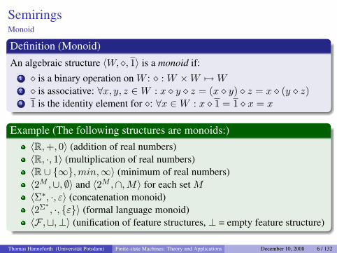
Definition (Monoid)An algebraic structure 〈W, �, 1〉 is a monoid if:

1 � is a binary operation on W : � : W ×W 7→W2 � is associative: ∀x, y, z ∈W : x � y � z = (x � y) � z = x � (y � z)3 1 is the identity element for �: ∀x ∈W : x � 1 = 1 � x = x

Example (The following structures are monoids:)〈R,+, 0〉 (addition of real numbers)〈R, ·, 1〉 (multiplication of real numbers)〈R ∪ {∞},min,∞〉 (minimum of real numbers)〈2M ,∪, ∅〉 and 〈2M ,∩,M〉 for each set M〈Σ∗, ·, ε〉 (concatenation monoid)〈2Σ∗ , ·, {ε}〉 (formal language monoid)〈F ,t,⊥〉 (unification of feature structures, ⊥ = empty feature structure)


SemiringsCommutative Monoid

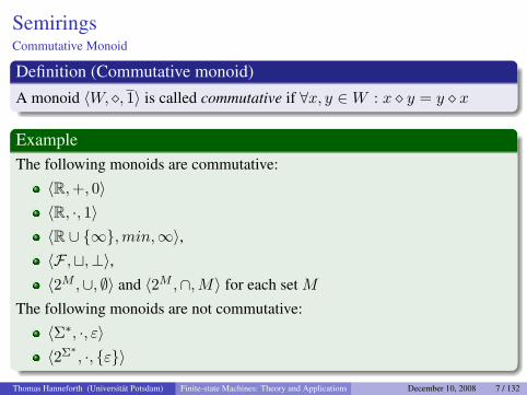
Definition (Commutative monoid)A monoid 〈W, �, 1〉 is called commutative if ∀x, y ∈W : x � y = y � x

ExampleThe following monoids are commutative:

〈R,+, 0〉〈R, ·, 1〉〈R ∪ {∞},min,∞〉,〈F ,t,⊥〉,〈2M ,∪, ∅〉 and 〈2M ,∩,M〉 for each set M

The following monoids are not commutative:

〈Σ∗, ·, ε〉〈2Σ∗ , ·, {ε}〉


SemiringsDefinition

Definition (Semiring)

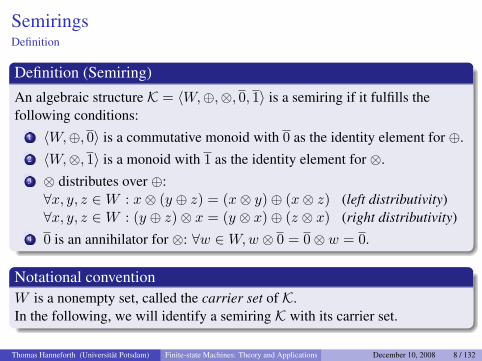
An algebraic structure K = 〈W,⊕,⊗, 0, 1〉 is a semiring if it fulfills thefollowing conditions:

1 〈W,⊕, 0〉 is a commutative monoid with 0 as the identity element for ⊕.2 〈W,⊗, 1〉 is a monoid with 1 as the identity element for ⊗.3 ⊗ distributes over ⊕:∀x, y, z ∈W : x⊗ (y ⊕ z) = (x⊗ y)⊕ (x⊗ z) (left distributivity)∀x, y, z ∈W : (y ⊕ z)⊗ x = (y ⊗ x)⊕ (z ⊗ x) (right distributivity)

4 0 is an annihilator for ⊗: ∀w ∈W,w ⊗ 0 = 0⊗ w = 0.

Notational conventionW is a nonempty set, called the carrier set of K.In the following, we will identify a semiring K with its carrier set.


SemiringsCommon semirings

Example (Common semirings)

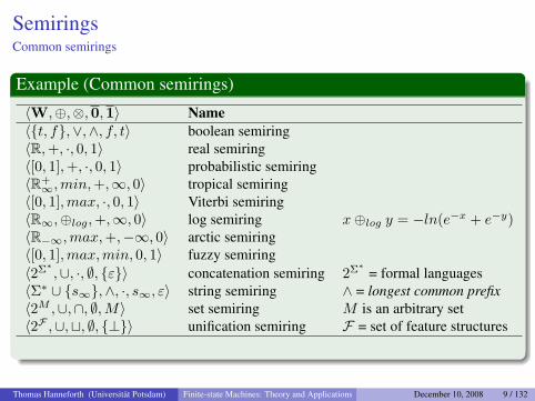
〈W,⊕,⊗,0,1〉 Name〈{t, f},∨,∧, f, t〉 boolean semiring〈R,+, ·, 0, 1〉 real semiring〈[0, 1],+, ·, 0, 1〉 probabilistic semiring〈R+∞,min,+,∞, 0〉 tropical semiring

〈[0, 1],max, ·, 0, 1〉 Viterbi semiring〈R∞,⊕log,+,∞, 0〉 log semiring x⊕log y = −ln(e−x + e−y)〈R−∞,max,+,−∞, 0〉 arctic semiring〈[0, 1],max,min, 0, 1〉 fuzzy semiring〈2Σ∗ ,∪, ·, ∅, {ε}〉 concatenation semiring 2Σ∗ = formal languages〈Σ∗ ∪ {s∞},∧, ·, s∞, ε〉 string semiring ∧ = longest common prefix〈2M ,∪,∩, ∅,M〉 set semiring M is an arbitrary set〈2F ,∪,t, ∅, {⊥}〉 unification semiring F = set of feature structures


SemiringsString semiring

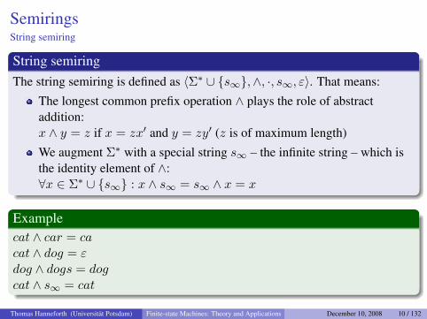
String semiringThe string semiring is defined as 〈Σ∗ ∪ {s∞},∧, ·, s∞, ε〉. That means:

The longest common prefix operation ∧ plays the role of abstractaddition:x ∧ y = z if x = zx′ and y = zy′ (z is of maximum length)

We augment Σ∗ with a special string s∞ – the infinite string – which isthe identity element of ∧:∀x ∈ Σ∗ ∪ {s∞} : x ∧ s∞ = s∞ ∧ x = x

Examplecat ∧ car = cacat ∧ dog = εdog ∧ dogs = dogcat ∧ s∞ = cat


SemiringsIsomorphic semirings

Definition (Isomorphic semirings)

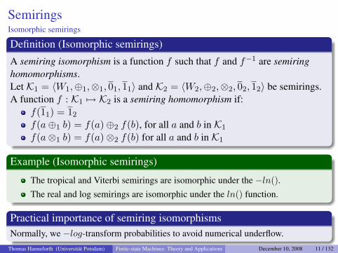
A semiring isomorphism is a function f such that f and f−1 are semiringhomomorphisms.Let K1 = 〈W1,⊕1,⊗1, 01, 11〉 and K2 = 〈W2,⊕2,⊗2, 02, 12〉 be semirings.A function f : K1 7→ K2 is a semiring homomorphism if:

f(11) = 12

f(a⊕1 b) = f(a)⊕2 f(b), for all a and b in K1

f(a⊗1 b) = f(a)⊗2 f(b) for all a and b in K1

Example (Isomorphic semirings)

The tropical and Viterbi semirings are isomorphic under the −ln().The real and log semirings are isomorphic under the ln() function.

Practical importance of semiring isomorphismsNormally, we −log-transform probabilities to avoid numerical underflow.


SemiringsOther interesting semirings: matrix semiring


SemiringsOther interesting semirings: entropy semiring


Outline

2 Weighted finite-state automata


Weighted finite-state automata

Weighted Finite-state AutomataWeighted finite-state acceptors

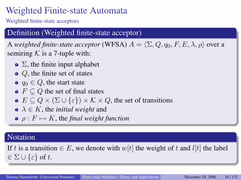
Definition (Weighted finite-state acceptor)A weighted finite-state acceptor (WFSA) A = 〈Σ, Q, q0, F, E, λ, ρ〉 over asemiring K is a 7-tuple with:

Σ, the finite input alphabetQ, the finite set of statesq0 ∈ Q, the start stateF ⊆ Q the set of final statesE ⊆ Q× (Σ ∪ {ε})×K ×Q, the set of transitionsλ ∈ K, the initial weight andρ : F 7→ K, the final weight function

NotationIf t is a transition ∈ E, we denote with w[t] the weight of t and l[t] the label∈ Σ ∪ {ε} of t.



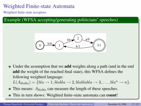
Example (WFSA accepting/generating politicians’ speeches)

� ��

��

��

��

��

Under the assumption that we add weights along a path (and in the endadd the weight of the reached final state), this WFSA defines thefollowing weighted language:L(Ablabla) = {bla→ 1, blabla→ 2, blablabla→ 3, . . . , blan → n}.This means: Ablabla can measure the length of these speeches.

This in turn shows: Weighted finite-state automata can count!



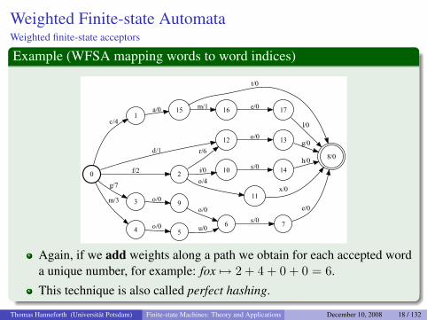
Example (WFSA mapping words to word indices)

�

��

��

��

��

�

�

�

��

��

��

��

��

��

��

��

��

��

��

��

��

��

�

��

��

��

��

��

��

��

��

Again, if we add weights along a path we obtain for each accepted worda unique number, for example: fox 7→ 2 + 4 + 0 + 0 = 6.

This technique is also called perfect hashing.


Weighted Finite-state AutomataWeighted finite-state transducers

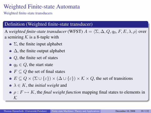
Definition (Weighted finite-state transducer)A weighted finite-state transducer (WFST) A = 〈Σ,∆, Q, q0, F, E, λ, ρ〉 overa semiring K is a 8-tuple with

Σ, the finite input alphabet

∆, the finite output alphabet

Q, the finite set of states

q0 ∈ Q, the start state

F ⊆ Q the set of final states

E ⊆ Q× (Σ ∪ {ε})× (∆ ∪ {ε})×K ×Q, the set of transitions

λ ∈ K, the initial weight and

ρ : F 7→ K, the final weight function mapping final states to elements inK


Weighted Finite-state AutomataWeighted finite-state transducers

Example


Weighted Finite-state AutomataWeight of a string - the Master formula

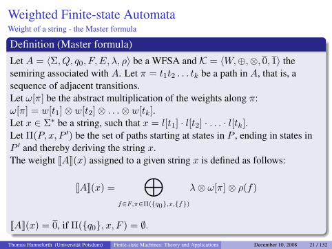
Definition (Master formula)Let A = 〈Σ, Q, q0, F, E, λ, ρ〉 be a WFSA and K = 〈W,⊕,⊗, 0, 1〉 thesemiring associated with A. Let π = t1t2 . . . tk be a path in A, that is, asequence of adjacent transitions.Let ω[π] be the abstract multiplication of the weights along π:ω[π] = w[t1]⊗ w[t2]⊗ . . .⊗ w[tk].Let x ∈ Σ∗ be a string, such that x = l[t1] · l[t2] · . . . · l[tk].Let Π(P, x, P ′) be the set of paths starting at states in P , ending in states inP ′ and thereby deriving the string x.The weight JAK(x) assigned to a given string x is defined as follows:

JAK(x) =⊕

f∈F,π∈Π({q0},x,{f})

λ⊗ ω[π]⊗ ρ(f)

JAK(x) = 0, if Π({q0}, x, F ) = ∅.


Weighted Finite-state AutomataWhat does the Master formula mean?

For each path labeled with x, starting at the start state and reaching afinal state, we combine a constant weight λ, the weight of the individualtransitions and the weight assigned to that final state by abstractmultiplication.

There may be more than one path for x, if A is non-deterministic.In that case, we abstractly add the weights of all paths.

This in turn means: if A is deterministic there is at most on path for x inA. The contribution of

⊕can then be neglected.

If there is no path for x, the weight assigned to x is 0.Thus, 0 – the identity element of ⊕ – signals, that a certain word x is notaccepted by A.

Note that JAK(x) is a function mapping x ∈ Σ∗ to elements in K.


Weighted Finite-state AutomataMaster formula

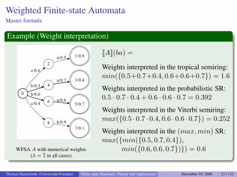
Example (Weight interpretation)

�

�

��

��

�

��

��

��

��

��

��

��

WFSA A with numerical weights(λ = 1 in all cases)

JAK(ba) =

Weights interpreted in the tropical semiring:min({0.5+0.7+0.4, 0.6+0.6+0.7}) = 1.6

Weights interpreted in the probabilistic SR:0.5 · 0.7 · 0.4 + 0.6 · 0.6 · 0.7 = 0.392

Weights interpreted in the Viterbi semiring:max({0.5 · 0.7 · 0.4, 0.6 · 0.6 · 0.7}) = 0.252

Weights interpreted in the (max,min) SR:max({min({0.5, 0.7, 0.4}),

min({0.6, 0.6, 0.7})}) = 0.6


Weighted Finite-state AutomataMaster formula

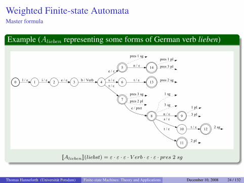
Example (Alieben representing some forms of German verb lieben)

� ��

��

��

��

��

��

�

��

� ��

��

��

� ��

� ��

�

��

� ��

� ��

� ��

��

��

��

��

��

��

��

��

��

��

��

��

JAliebenK(liebst) = ε · ε · ε · V erb · ε · ε · pres 2 sg


Weighted Finite-state AutomataWhy are semirings a suitable weight structure for finite-state automata?

The fact that the semiring is composed out of two monoids gives us:I two identity elements 0 and 1: 0 signals that some string is not part of the

language accepted by the WFSM, and 1, which gives us a notion of a“trivial” weight

I a high degree of freedom in which order to compute weights (byassociativity)

Commutativity of ⊕ gives us the freedom to consider the paths accordingto the master formula in any order

Distributivity of ⊗ enables us to factor out common “weight prefixes” ofdifferent paths (this property is for example important for weighteddeterminization)

The annihilation relationship between ⊗ and 0 causes any path whichcontains a transition with weight 0 to be invalid


Weighted Finite-state AutomataSignificance of semirings

Semirings play an import role in processing tasks based on finite-stateautomata, but are not limited to that.

The tropical semiring is the classical semiring of all kinds ofshortest-distance / best-analysis problems

The probabilistic semiring plays a important role in statistical languageprocessing for computing string probabilities.

The same is true for the Viterbi semiring, since it is related to processingtasks where we are interested in the analysis with the highest probability.

The string semiring is used in string processing tasks, computationalmorphology.


Weighted Finite-state AutomataWeighted rational languages

Weighted rational languages as monoid homomorphisms


Weighted Finite-state AutomataWeighted regular relations

Definition (Weighted regular relation)1

2


Outline

3 Semiring properties


Semiring properties

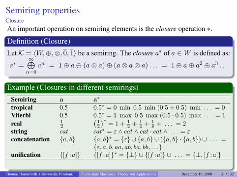
Semiring propertiesClosureAn important operation on semiring elements is the closure operation ∗.

Definition (Closure)Let K = 〈W,⊕,⊗, 0, 1〉 be a semiring. The closure a∗ of a ∈W is defined as:

a∗ =∞⊕n=0

an = 1⊕ a⊕ (a⊗ a)⊕ (a⊗ a⊗ a) . . . = 1⊕ a⊕ a2 ⊕ a3 . . .

Example (Closures in different semirings)Semiring a a∗

tropical 0.5 0.5∗ = 0 min 0.5 min (0.5 + 0.5) min . . . = 0Viterbi 0.5 0.5∗ = 1 max 0.5 max (0.5 · 0.5) max . . . = 1real 1

2

(12

)∗ = 1 + 12 + 1

4 + 18 + . . . = 2

string cat cat∗ = ε ∧ cat ∧ cat · cat ∧ . . . = εconcatenation {a, b} {a, b}∗ = {ε} ∪ {a, b} ∪ ({a, b} · {a, b}) ∪ . . . =

{ε, a, b, aa, ab, ba, bb, . . .}unification {[f :a]} {[f :a]}∗ = {⊥} ∪ {[f :a]} ∪ . . . = {⊥, [f :a]}


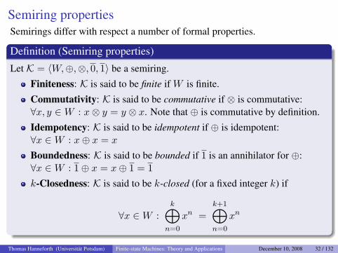
Semiring propertiesSemirings differ with respect a number of formal properties.

Definition (Semiring properties)

Let K = 〈W,⊕,⊗, 0, 1〉 be a semiring.

Finiteness: K is said to be finite if W is finite.

Commutativity: K is said to be commutative if ⊗ is commutative:∀x, y ∈W : x⊗ y = y ⊗ x. Note that ⊕ is commutative by definition.

Idempotency: K is said to be idempotent if ⊕ is idempotent:∀x ∈W : x⊕ x = x

Boundedness: K is said to be bounded if 1 is an annihilator for ⊕:∀x ∈W : 1⊕ x = x⊕ 1 = 1k-Closedness: K is said to be k-closed (for a fixed integer k) if

∀x ∈W :k⊕

n=0

xn =k+1⊕n=0

xn


Semiring properties

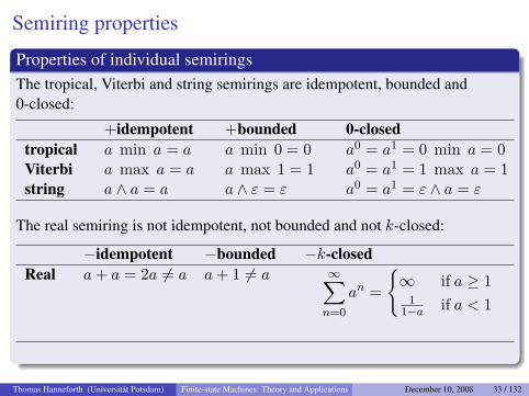
Properties of individual semiringsThe tropical, Viterbi and string semirings are idempotent, bounded and0-closed:

+idempotent +bounded 0-closedtropical a min a = a a min 0 = 0 a0 = a1 = 0 min a = 0Viterbi a max a = a a max 1 = 1 a0 = a1 = 1 max a = 1string a ∧ a = a a ∧ ε = ε a0 = a1 = ε ∧ a = ε

The real semiring is not idempotent, not bounded and not k-closed:

−idempotent −bounded −k-closedReal a+ a = 2a 6= a a+ 1 6= a ∞∑

n=0

an =

{∞ if a ≥ 1

11−a if a < 1


Semiring properties

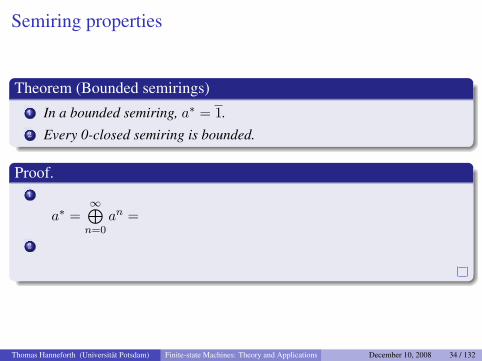
Theorem (Bounded semirings)1 In a bounded semiring, a∗ = 1.2 Every 0-closed semiring is bounded.

Proof.1

a∗ =∞⊕n=0

an =

2


Semiring propertiesClosed semiring

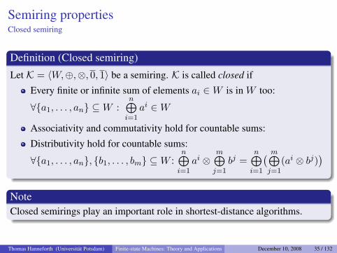
Definition (Closed semiring)

Let K = 〈W,⊕,⊗, 0, 1〉 be a semiring. K is called closed if

Every finite or infinite sum of elements ai ∈W is in W too:

∀{a1, . . . , an} ⊆W :n⊕i=1

ai ∈W

Associativity and commutativity hold for countable sums:

Distributivity hold for countable sums:

∀{a1, . . . , an}, {b1, . . . , bm} ⊆W :n⊕i=1

ai ⊗m⊕j=1

bj =n⊕i=1

( m⊕j=1

(ai ⊗ bj))

NoteClosed semirings play an important role in shortest-distance algorithms.


Semiring properties

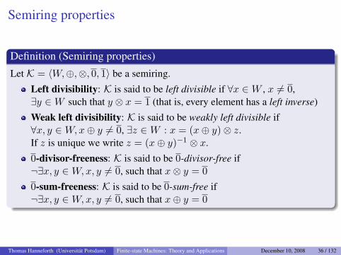
Definition (Semiring properties)

Let K = 〈W,⊕,⊗, 0, 1〉 be a semiring.

Left divisibility: K is said to be left divisible if ∀x ∈W , x 6= 0,∃y ∈W such that y ⊗ x = 1 (that is, every element has a left inverse)

Weak left divisibility: K is said to be weakly left divisible if∀x, y ∈W,x⊕ y 6= 0, ∃z ∈W : x = (x⊕ y)⊗ z.If z is unique we write z = (x⊕ y)−1 ⊗ x.

0-divisor-freeness: K is said to be 0-divisor-free if¬∃x, y ∈W,x, y 6= 0, such that x⊗ y = 00-sum-freeness: K is said to be 0-sum-free if¬∃x, y ∈W,x, y 6= 0, such that x⊕ y = 0


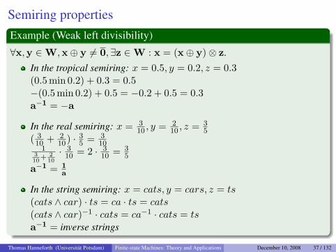
Semiring propertiesExample (Weak left divisibility)

∀x,y ∈W,x⊕ y 6= 0, ∃z ∈W : x = (x⊕ y)⊗ z.

In the tropical semiring: x = 0.5, y = 0.2, z = 0.3(0.5 min 0.2) + 0.3 = 0.5−(0.5 min 0.2) + 0.5 = −0.2 + 0.5 = 0.3a−1 = −a

In the real semiring: x = 310 , y = 2

10 , z = 35

( 310 + 2

10) · 35 = 3

101

310

+ 210

· 310 = 2 · 3

10 = 35

a−1 = 1a

In the string semiring: x = cats, y = cars, z = ts(cats ∧ car) · ts = ca · ts = cats(cats ∧ car)−1 · cats = ca−1 · cats = tsa−1 = inverse strings


Semiring propertiesWeak left divisibility and determinization of WFSAs

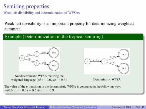
Weak left divisibility is an important property for determinizing weightedautomata.

Example (Determinization in the tropical semiring)

�

��

�

��

��

��

��

Nondeterministic WFSA realizing theweighted language {ab 7→ 0.9, ac 7→ 0.6}

� ��

��

��

��

Deterministic WFSA

The value of the c-transition in the deterministic WFSA is computed in the following way:−(0.5 min 0.3) + 0.5 + 0.1 = 0.3


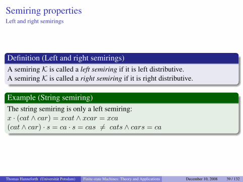
Semiring propertiesLeft and right semirings

Definition (Left and right semirings)A semiring K is called a left semiring if it is left distributive.A semiring K is called a right semiring if it is right distributive.

Example (String semiring)The string semiring is only a left semiring:x · (cat ∧ car) = xcat ∧ xcar = xca(cat ∧ car) · s = ca · s = cas 6= cats ∧ cars = ca


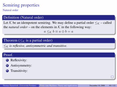
Semiring propertiesNatural order

Definition (Natural order)Let K be an idempotent semiring. We may define a partial order ≤K – calledthe natural order – on the elements in K in the following way:

a ≤K b ≡ a⊕ b = a

Theorem (≤K is a partial order)≤K is reflexive, antisymmetric and transitive.

Proof.1 Reflexivity:2 Antisymmetry:3 Transitivity:


Semiring propertiesNatural order

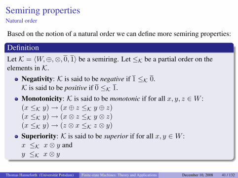
Based on the notion of a natural order we can define more semiring properties:

DefinitionLet K = 〈W,⊕,⊗, 0, 1〉 be a semiring. Let ≤K be a partial order on theelements in K.

Negativity: K is said to be negative if 1 ≤K 0.K is said to be positive if 0 ≤K 1.

Monotonicity: K is said to be monotonic if for all x, y, z ∈W :(x ≤K y)→ (x⊕ z ≤K y ⊕ z)(x ≤K y)→ (x⊗ z ≤K y ⊗ z)(x ≤K y)→ (z ⊗ x ≤K z ⊗ y)Superiority: K is said to be superior if for all x, y ∈W :x ≤K x⊗ y andy ≤K x⊗ y


Semiring propertiesNatural order: significance

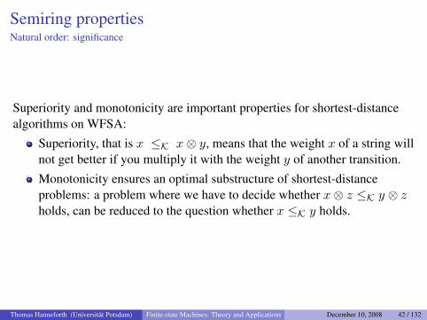
Superiority and monotonicity are important properties for shortest-distancealgorithms on WFSA:

Superiority, that is x ≤K x⊗ y, means that the weight x of a string willnot get better if you multiply it with the weight y of another transition.

Monotonicity ensures an optimal substructure of shortest-distanceproblems: a problem where we have to decide whether x⊗ z ≤K y ⊗ zholds, can be reduced to the question whether x ≤K y holds.


Semiring properties

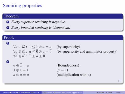
Theorem1 Every superior semiring is negative.2 Every bounded semiring is idempotent.

Proof.1

∀a ∈ K : 1 ≤ 1⊗ a = a (by superiority)∀a ∈ K : a ≤ 0⊗ a = 0 (by superiority and annihilator property)∀a ∈ K : 1 ≤ a ≤ 0

2

a⊕ 1 = a (Boundedness)1⊕ 1 = 1 (a = 1)a⊕ a = a (multiplication with a)


Semiring propertiesSummary: Semirings and their properties

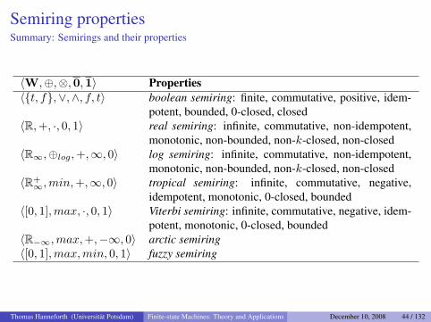
〈W,⊕,⊗,0,1〉 Properties〈{t, f},∨,∧, f, t〉 boolean semiring: finite, commutative, positive, idem-

potent, bounded, 0-closed, closed〈R,+, ·, 0, 1〉 real semiring: infinite, commutative, non-idempotent,

monotonic, non-bounded, non-k-closed, non-closed〈R∞,⊕log,+,∞, 0〉 log semiring: infinite, commutative, non-idempotent,

monotonic, non-bounded, non-k-closed, non-closed〈R+∞,min,+,∞, 0〉 tropical semiring: infinite, commutative, negative,

idempotent, monotonic, 0-closed, bounded〈[0, 1],max, ·, 0, 1〉 Viterbi semiring: infinite, commutative, negative, idem-

potent, monotonic, 0-closed, bounded〈R−∞,max,+,−∞, 0〉 arctic semiring〈[0, 1],max,min, 0, 1〉 fuzzy semiring


Semiring propertiesSummary: Semirings and their properties

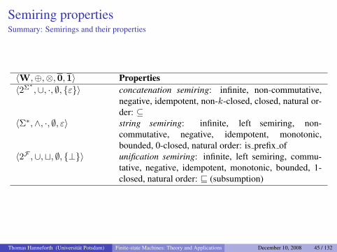
〈W,⊕,⊗,0,1〉 Properties〈2Σ∗ ,∪, ·, ∅, {ε}〉 concatenation semiring: infinite, non-commutative,

negative, idempotent, non-k-closed, closed, natural or-der: ⊆

〈Σ∗,∧, ·, ∅, ε〉 string semiring: infinite, left semiring, non-commutative, negative, idempotent, monotonic,bounded, 0-closed, natural order: is prefix of

〈2F ,∪,t, ∅, {⊥}〉 unification semiring: infinite, left semiring, commu-tative, negative, idempotent, monotonic, bounded, 1-closed, natural order: v (subsumption)


Semiring propertiesSemiring properties and FSM algebra

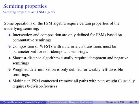
Some operations of the FSM algebra require certain properties of theunderlying semiring:

Intersection and composition are only defined for FSMs based oncommutative semirings.

Composition of WFSTs with ε : x or x : ε transitions must beparameterized for non-idempotent semirings.

Shortest-distance algorithms usually require idempotent and negativesemirings

Weighted determinization is only defined for weakly left-divisiblesemirings.

Making an FSM connected (remove all paths with path weight 0) usuallyrequires 0-divisor-freeness


Outline

4 Closure properties and algebra of weighted finite-state automataWeighted closureWeighted intersectionWeighted compositionAlgebra of WRLs and WRTs


Closure properties and algebra

of weighted finite-state automata

Closure properties and algebra of WFSA

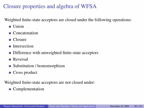
Weighted finite-state acceptors are closed under the following operations:

Union

Concatenation

Closure

Intersection

Difference with unweighted finite-state acceptors

Reversal

Substitution / homomorphism

Cross product

Weighted finite-state acceptors are not closed under:

Complementation


Closure properties and algebra of WFSM

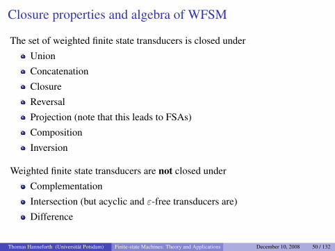
The set of weighted finite state transducers is closed under

Union

Concatenation

Closure

Reversal

Projection (note that this leads to FSAs)

Composition

Inversion

Weighted finite state transducers are not closed under

Complementation

Intersection (but acyclic and ε-free transducers are)

Difference


Closure properties and algebra of WFSAWeighted closure

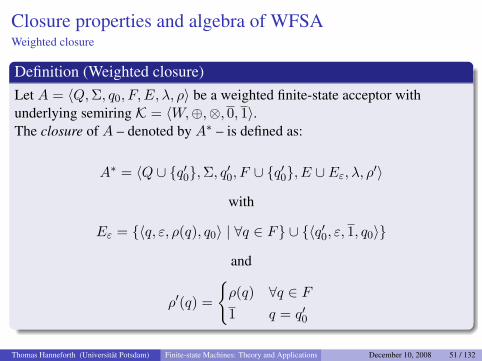
Definition (Weighted closure)Let A = 〈Q,Σ, q0, F, E, λ, ρ〉 be a weighted finite-state acceptor withunderlying semiring K = 〈W,⊕,⊗, 0, 1〉.The closure of A – denoted by A∗ – is defined as:

A∗ = 〈Q ∪ {q′0},Σ, q′0, F ∪ {q′0}, E ∪ Eε, λ, ρ′〉

with

Eε = {〈q, ε, ρ(q), q0〉 | ∀q ∈ F} ∪ {〈q′0, ε, 1, q0〉}

and

ρ′(q) =

{ρ(q) ∀q ∈ F1 q = q′0


Closure properties and algebra of WFSAWeighted closure

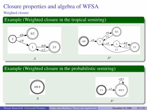
Example (Weighted closure in the tropical semiring)

��

� ��

��

�

��

��

A

��

��

��

��

��

��

��

��

��

A∗

Example (Weighted closure in the probabilistic semiring)

��

A

��

��

��

A∗


Closure properties and algebra of WFSAWeighted intersection

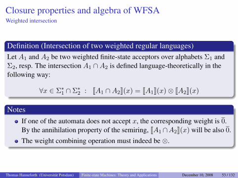
Definition (Intersection of two weighted regular languages)Let A1 and A2 be two weighted finite-state acceptors over alphabets Σ1 andΣ2, resp. The intersection A1 ∩A2 is defined language-theoretically in thefollowing way:

∀x ∈ Σ∗1 ∩ Σ∗2 : JA1 ∩A2K(x) = JA1K(x)⊗ JA2K(x)

NotesIf one of the automata does not accept x, the corresponding weight is 0.By the annihilation property of the semiring, JA1∩A2K(x) will be also 0.

The weight combining operation must indeed be ⊗.



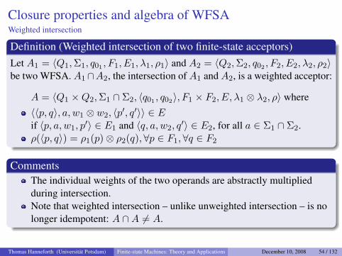
Definition (Weighted intersection of two finite-state acceptors)Let A1 = 〈Q1,Σ1, q01 , F1, E1, λ1, ρ1〉 and A2 = 〈Q2,Σ2, q02 , F2, E2, λ2, ρ2〉be two WFSA. A1∩A2, the intersection of A1 and A2, is a weighted acceptor:

A = 〈Q1 ×Q2,Σ1 ∩ Σ2, 〈q01 , q02〉, F1 × F2, E, λ1 ⊗ λ2, ρ〉 where

〈〈p, q〉, a, w1 ⊗ w2, 〈p′, q′〉〉 ∈ Eif 〈p, a, w1, p

′〉 ∈ E1 and 〈q, a, w2, q′〉 ∈ E2, for all a ∈ Σ1 ∩ Σ2.

ρ(〈p, q〉) = ρ1(p)⊗ ρ2(q),∀p ∈ F1, ∀q ∈ F2

CommentsThe individual weights of the two operands are abstractly multipliedduring intersection.Note that weighted intersection – unlike unweighted intersection – is nolonger idempotent: A ∩A 6= A.



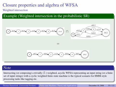
Example (Weighted intersection in the probabilistic SR)

� �� ∩�

��

��

��

��

��

��

��

=

� ��

NoteIntersecting (or composing) a trivially (1-) weighted, acyclic WFSA representing an input string (or a finiteset of input strings) with a cyclic weighted finite-state machine is the typical scenario for HMM-styleprocessing tasks like tagging etc.


Closure properties and algebra of WFSAWeighted intersection: why is it only possible in commutative semirings?

1 Let A1 and A2 be two ε-free WFSA.2 Suppose that some input x is in A1 ∩A2 with JA1 ∩A2K(x) 6= 0.3 Let t11 . . . t

1n and t21 . . . t

2n be accepting paths in A1 and A2, respectively

4 The algebraic definition of intersection is:JA1 ∩A2K(x) = (JA1K(x)⊗ JA2K(x).In our example that means:JA1 ∩A2K(x) = (w[t11]⊗ . . .⊗ w[t1n])⊗ (w[t21]⊗ . . .⊗ w[t2n])

5 The weight of the corresponding path in A1 ∩A2 is(w[t11]⊗ w[t21])⊗ (w[t12]⊗ w[t22])⊗ . . .⊗ (w[t1n]⊗ w[t2n])

6 But 4. and 5. are the same only if the underlying semiring of A1 and A2

is commutative.


Closure properties and algebra of WFSAWeighted intersection in non-commutative semirings?

This result limits the usefulness of intersection and composition innon-commutative semirings like the string semiring.

On the other hand, if one of the operands in A1 ∩A2 is triviallyweighted, then no problem arises.


Closure properties and algebra of WFSAWeighted composition

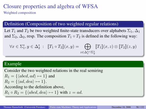
Definition (Composition of two weighted regular relations)Let T1 and T2 be two weighted finite-state transducers over alphabets Σ1, ∆1

and Σ2, ∆2, resp. The composition T1 ◦ T2 is defined in the following way:

∀x ∈ Σ∗1, y ∈ ∆∗2 : JT1 ◦ T2K(x, y) =⊕

z∈∆∗1∩Σ∗2

JT1K(x, z)⊗ JT2K(z, y)

ExampleConsider the two weighted relations in the real semiringR1 = {〈abcd, ad〉 7→ 1} andR2 = {〈ad, dea〉 7→ 1}.According to the definition above,R1 ◦R2 = {〈abcd, dea〉 7→ 1} with z = ad.



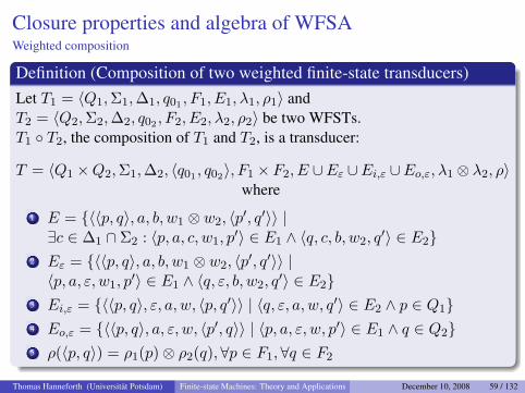
Definition (Composition of two weighted finite-state transducers)Let T1 = 〈Q1,Σ1,∆1, q01 , F1, E1, λ1, ρ1〉 andT2 = 〈Q2,Σ2,∆2, q02 , F2, E2, λ2, ρ2〉 be two WFSTs.T1 ◦ T2, the composition of T1 and T2, is a transducer:

T = 〈Q1 ×Q2,Σ1,∆2, 〈q01 , q02〉, F1 × F2, E ∪Eε ∪Ei,ε ∪Eo,ε, λ1 ⊗ λ2, ρ〉where

1 E = {〈〈p, q〉, a, b, w1 ⊗ w2, 〈p′, q′〉〉 |∃c ∈ ∆1 ∩ Σ2 : 〈p, a, c, w1, p

′〉 ∈ E1 ∧ 〈q, c, b, w2, q′〉 ∈ E2}

2 Eε = {〈〈p, q〉, a, b, w1 ⊗ w2, 〈p′, q′〉〉 |〈p, a, ε, w1, p

′〉 ∈ E1 ∧ 〈q, ε, b, w2, q′〉 ∈ E2}

3 Ei,ε = {〈〈p, q〉, ε, a, w, 〈p, q′〉〉 | 〈q, ε, a, w, q′〉 ∈ E2 ∧ p ∈ Q1}4 Eo,ε = {〈〈p, q〉, a, ε, w, 〈p′, q〉〉 | 〈p, a, ε, w, p′〉 ∈ E1 ∧ q ∈ Q2}5 ρ(〈p, q〉) = ρ1(p)⊗ ρ2(q),∀p ∈ F1, ∀q ∈ F2



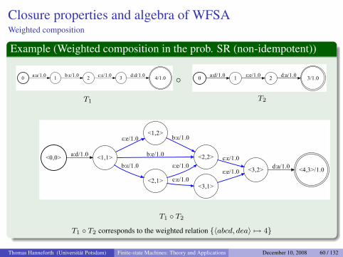
Example (Weighted composition in the prob. SR (non-idempotent))

� ��

��

��

��

T1

◦ � ��

��

��

T2

��

��

��

��

��

��

��

��

��

��

T1 ◦ T2

T1 ◦ T2 corresponds to the weighted relation {〈abcd, dea〉 7→ 4}


Closure properties and algebra of WFSAWeighted composition: ε-filter FSTs

The problem is, that there are 4 paths deriving the string pair bc : e withweight 1.0

By the master formula, paths weights are added

In idempotent semirings this doesn’t cause harm, since a⊕ a = a.But in non-idempotent semirings, we are faced with a problem

Solution: introduce a filter such that all paths except one are deleted



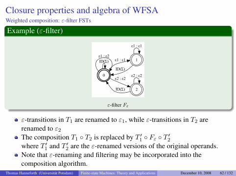
Example (ε-filter)

�

��

��

��

��

��

��

��

ε-filter Fε

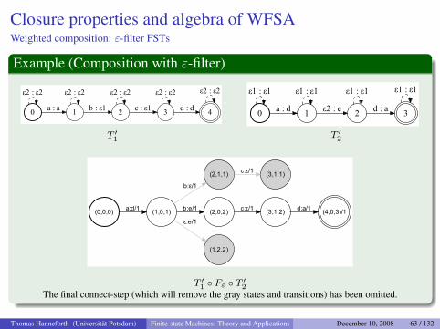
ε-transitions in T1 are renamed to ε1, while ε-transitions in T2 arerenamed to ε2

The composition T1 ◦ T2 is replaced by T ′1 ◦ Fε ◦ T ′2where T ′1 and T ′2 are the ε-renamed versions of the original operands.Note that ε-renaming and filtering may be incorporated into thecomposition algorithm.



Example (Composition with ε-filter)

�

��

��

��

��

��

��

��

��

��

T ′1

�

��

��

��

��

��

��

��

T ′2

��

��

��

��

��

��

� ��

� ��

��

T ′1 ◦ Fε ◦ T ′2The final connect-step (which will remove the gray states and transitions) has been omitted.


Closure properties and algebra of WFSAAlgebra of WRLs and WRTs

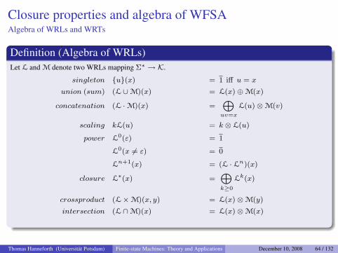
Definition (Algebra of WRLs)Let L and M denote two WRLs mapping Σ∗ → K.

singleton {u}(x) = 1 iff u = x

union (sum) (L ∪M)(x) = L(x)⊕M(x)

concatenation (L ·M)(x) =⊕uv=x

L(u)⊗M(v)

scaling kL(u) = k ⊗ L(u)

power L0(ε) = 1

L0(x 6= ε) = 0

Ln+1(x) = (L · Ln)(x)

closure L∗(x) =⊕k≥0

Lk(x)

crossproduct (L×M)(x, y) = L(x)⊗M(y)

intersection (L ∩M)(x) = L(x)⊗M(x)



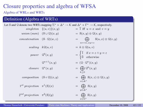
Definition (Algebra of WRTs)Let S and Q denote two WRTs mapping Σ∗ ×∆∗ → K and ∆∗ × Γ∗ → K, respectively.

singleton {(u, v)}(x, y) = 1 iff u = x and v = y

union (sum) (S ∪ Q)(x, y) = S(x, y)⊕ Q(x, y)

concatenation (S · Q)(w, z) =⊕

uv=w,xy=z

S(u, x)⊗ Q(v, y)

scaling kQ(u, v) = k ⊗ Q(u, v)

power Q0(x, y) =

{1 if x = ε ∧ y = ε

0 otherwise

Qn+1(x, y) = (Q · Qn)(x, y)

closure Q∗(x, y) =⊕k≥0

Qk(x, y)

composition (S ◦ Q)(x, y) =⊕z∈∆∗

S(x, z)⊗ Q(z, y)

1st projection π1(S)(x) =⊕y∈∆∗

S(x, y)

2nd projection π2(S)(y) =⊕x∈Σ∗

S(x, y)



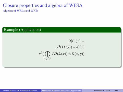
Example (Application)

Q[L](x) =

π2(ID(L) ◦ Q)(x)

π2(⊕x∈∆∗

ID(L(x))⊗ Q(x, y))


Outline

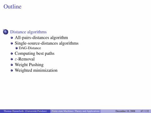
5 Distance algorithmsAll-pairs-distances algorithmSingle-source-distances algorithms

DAG-Distance

Computing best pathsε-RemovalWeight PushingWeighted minimization


Distance algorithms

in weighted finite-state automata

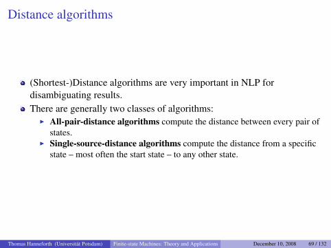
Distance algorithms

(Shortest-)Distance algorithms are very important in NLP fordisambiguating results.There are generally two classes of algorithms:

I All-pair-distance algorithms compute the distance between every pair ofstates.

I Single-source-distance algorithms compute the distance from a specificstate – most often the start state – to any other state.


Distance algorithms

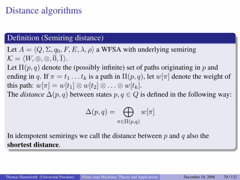
Definition (Semiring distance)Let A = 〈Q,Σ, q0, F, E, λ, ρ〉 a WFSA with underlying semiringK = 〈W,⊕,⊗, 0, 1〉.Let Π(p, q) denote the (possibly infinite) set of paths originating in p andending in q. If π = t1 . . . tk is a path in Π(p, q), let w[π] denote the weight ofthis path: w[π] = w[t1]⊗ w[t2]⊗ . . .⊗ w[tk].The distance ∆(p, q) between states p, q ∈ Q is defined in the following way:

∆(p, q) =⊕

π∈Π(p,q)

w[π]

In idempotent semirings we call the distance between p and q also theshortest distance.


Distance algorithmsClosed semiring: recapitulation of the definition

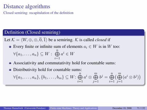
Definition (Closed semiring)

Let K = 〈W,⊕,⊗, 0, 1〉 be a semiring. K is called closed if

Every finite or infinite sum of elements ai ∈W is in W too:

∀{a1, . . . , an} ⊆W :n⊕i=1

ai ∈W

Associativity and commutativity hold for countable sums:

Distributivity hold for countable sums:

∀{a1, . . . , an}, {b1, . . . , bm} ⊆W :n⊕i=1

ai ⊗m⊕j=1

bj =n⊕i=1

( m⊕j=1

(ai ⊗ bj))


Distance algorithmsAll-pairs-distances algorithm

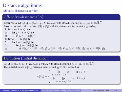
All-pairs-distances(A)

Require: A WFSA A = 〈Q,Σ, q0, F, E, λ, ρ〉 with closed semiring K = 〈W,⊕,⊗, 0, 1〉Ensure: A matrix d|Q| of size |Q| × |Q| with the distances between states qi and qj .1: for i← 1 to |Q| do2: for j ← 1 to |Q| do3: d0[i, j]← w[i, j]4: for k ← 1 to |Q| do5: for i← 1 to |Q| do6: for j ← 1 to |Q| do7: d(k)[i, j]← d(k−1)[i, j]⊕

(d(k−1)[i, k]⊗ (d(k−1)[k, k])∗ ⊗ d(k−1)[k, j]

)Definition (Initial distance)Let A = 〈Q,Σ, q0, F, E, λ, ρ〉 a WFSA with closed semiring K = 〈W,⊕,⊗, 0, 1〉.The initial distance w[i, j] between states qi and qj ∈ Q is defined as:

w[i, j] =

⊕

〈qi,a,w,qj〉∈Ew if i 6= j

1⊕⊕

〈qi,a,w,qj〉∈Ew if i = j


Distance algorithmsAll-pairs-distance algorithm

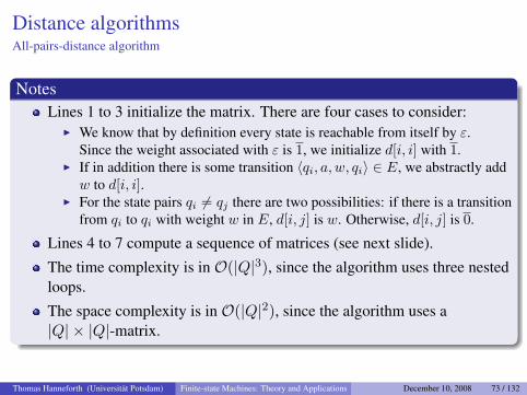
NotesLines 1 to 3 initialize the matrix. There are four cases to consider:

I We know that by definition every state is reachable from itself by ε.Since the weight associated with ε is 1, we initialize d[i, i] with 1.

I If in addition there is some transition 〈qi, a, w, qi〉 ∈ E, we abstractly addw to d[i, i].

I For the state pairs qi 6= qj there are two possibilities: if there is a transitionfrom qi to qi with weight w in E, d[i, j] is w. Otherwise, d[i, j] is 0.

Lines 4 to 7 compute a sequence of matrices (see next slide).

The time complexity is in O(|Q|3), since the algorithm uses three nestedloops.

The space complexity is in O(|Q|2), since the algorithm uses a|Q| × |Q|-matrix.


Distance algorithmsAll-pairs-distance algorithm: idea

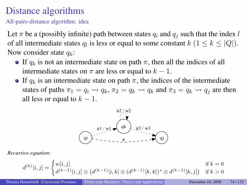
Let π be a (possibly infinite) path between states qi and qj such that the index lof all intermediate states ql is less or equal to some constant k (1 ≤ k ≤ |Q|).Now consider state qk:

If qk is not an intermediate state on path π, then all the indices of allintermediate states on π are less or equal to k − 1.If qk is an intermediate state on path π, the indices of the intermediatestates of paths π1 = qi qk, π2 = qk qk and π3 = qk qj are thenall less or equal to k − 1.

��

��

��

��

��

Recursive equation:

d(k)[i, j] =

{w[i, j] if k = 0

d(k−1)[i, j]⊕(d(k−1)[i, k]⊗ (d(k−1)[k, k])∗ ⊗ d(k−1)[k, j]

)if k > 0


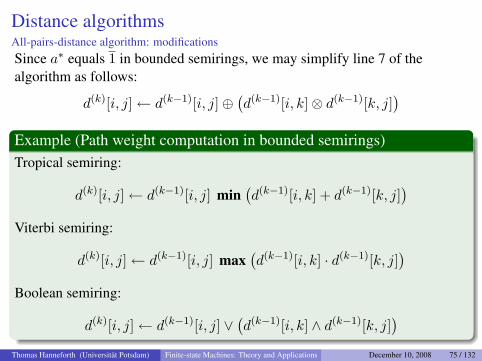
Distance algorithmsAll-pairs-distance algorithm: modificationsSince a∗ equals 1 in bounded semirings, we may simplify line 7 of thealgorithm as follows:

d(k)[i, j]← d(k−1)[i, j]⊕(d(k−1)[i, k]⊗ d(k−1)[k, j]

)Example (Path weight computation in bounded semirings)Tropical semiring:

d(k)[i, j]← d(k−1)[i, j] min(d(k−1)[i, k] + d(k−1)[k, j]

)Viterbi semiring:

d(k)[i, j]← d(k−1)[i, j] max(d(k−1)[i, k] · d(k−1)[k, j]

)Boolean semiring:

d(k)[i, j]← d(k−1)[i, j] ∨(d(k−1)[i, k] ∧ d(k−1)[k, j]

)Thomas Hanneforth (Universitat Potsdam) Finite-state Machines: Theory and Applications December 10, 2008 75 / 132

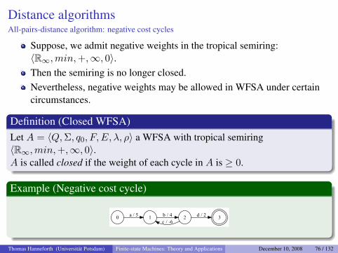
Distance algorithmsAll-pairs-distance algorithm: negative cost cycles

Suppose, we admit negative weights in the tropical semiring:〈R∞,min,+,∞, 0〉.Then the semiring is no longer closed.Nevertheless, negative weights may be allowed in WFSA under certaincircumstances.

Definition (Closed WFSA)Let A = 〈Q,Σ, q0, F, E, λ, ρ〉 a WFSA with tropical semiring〈R∞,min,+,∞, 0〉.A is called closed if the weight of each cycle in A is ≥ 0.

Example (Negative cost cycle)

� ��

��


Distance algorithmsAll-pairs-distance algorithm

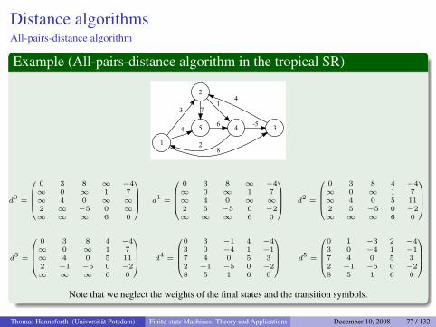
Example (All-pairs-distance algorithm in the tropical SR)

�

��

�

�

�

�

��

��

�

��

�

d0

=

0 3 8 ∞ −4∞ 0 ∞ 1 7∞ 4 0 ∞ ∞2 ∞ −5 0 ∞∞ ∞ ∞ 6 0

d1

=

0 3 8 ∞ −4∞ 0 ∞ 1 7∞ 4 0 ∞ ∞2 5 −5 0 −2∞ ∞ ∞ 6 0

d2

=

0 3 8 4 −4∞ 0 ∞ 1 7∞ 4 0 5 112 5 −5 0 −2∞ ∞ ∞ 6 0

d3

=

0 3 8 4 −4∞ 0 ∞ 1 7∞ 4 0 5 112 −1 −5 0 −2∞ ∞ ∞ 6 0

d4

=

0 3 −1 4 −43 0 −4 1 −17 4 0 5 32 −1 −5 0 −28 5 1 6 0

d5

=

0 1 −3 2 −43 0 −4 1 −17 4 0 5 32 −1 −5 0 −28 5 1 6 0

Note that we neglect the weights of the final states and the transition symbols.


Distance algorithmsAll-pairs-distance algorithm and matrix multiplication


Distance algorithmsAll-pairs-distance algorithm: applications

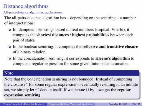
The all-pairs-distance algorithm has – depending on the semiring – a numberof interpretations:

In idempotent semirings based on real numbers (tropical, Viterbi), itcomputes the shortest distances / highest probabilities between eachpair of states.

In the boolean semiring, it computes the reflexive and transitive closureof a binary relation.

In the concatenation semiring, it corresponds to Kleene’s algorithm tocompute a regular expression for some given finite-state automaton.

NoteNote that the concatenation semiring is not bounded. Instead of computingthe closure r∗ for some regular expression r, eventually resulting in an infiniteset, we simply let r∗ denote itself. If we denote ∪ by |, we get the regularexpression semiring.


Distance algorithmsAll-pairs-distance algorithm: Kleene’s algorithm

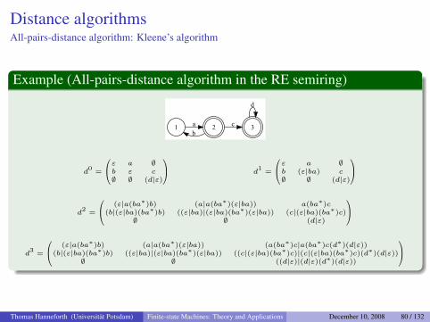
Example (All-pairs-distance algorithm in the RE semiring)

� ��

��

�

d0

=

ε a ∅b ε c∅ ∅ (d|ε)

d1

=

ε a ∅b (ε|ba) c∅ ∅ (d|ε)

d2

=

(ε|a(ba∗)b) (a|a(ba∗)(ε|ba)) a(ba∗)c(b|(ε|ba)(ba∗)b) ((ε|ba)|(ε|ba)(ba∗)(ε|ba)) (c|(ε|ba)(ba∗)c)

∅ ∅ (d|ε)

d3

=

(ε|a(ba∗)b) (a|a(ba∗)(ε|ba)) (a(ba∗)c|a(ba∗)c(d∗)(d|ε))(b|(ε|ba)(ba∗)b) ((ε|ba)|(ε|ba)(ba∗)(ε|ba)) ((c|(ε|ba)(ba∗)c)|(c|(ε|ba)(ba∗)c)(d∗)(d|ε))

∅ ∅ ((d|ε)|(d|ε)(d∗)(d|ε))


Distance algorithmsAll-pairs-distance algorithm: Kleene’s algorithm

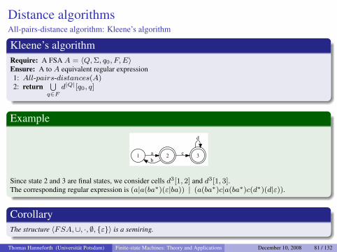
Kleene’s algorithmRequire: A FSA A = 〈Q,Σ, q0, F, E〉Ensure: A to A equivalent regular expression1: All-pairs-distances(A)2: return

⋃q∈F

d|Q|[q0, q]

Example

� ��

��

�

Since state 2 and 3 are final states, we consider cells d3[1, 2] and d3[1, 3].The corresponding regular expression is (a|a(ba∗)(ε|ba)) | (a(ba∗)c|a(ba∗)c(d∗)(d|ε)).

CorollaryThe structure 〈FSA,∪, ·, ∅, {ε}〉 is a semiring.


Distance algorithmsSingle-source-distance algorithms

Single-source-distance algorithms compute the distances from a givenstate q (in most cases the start state q0) to every other state in the WFSA.They have a lot of applications:

I Computing the best analysis (tropical semiring)I Computing the path with the highest probability (Viterbi semiring)I Statistical language processing: forward algorithm (probabilistic semiring)

There are a number of different algorithms, depending of the acyclicityof the input WFSA and the semiring:

1 Lawler’s algorithm2 Dijkstra’s algorithm3 Bellman-Ford algorithm4 Mohri’s algorithm

Mohri’s algorithm generalizes algorithms 1 to 3.


Distance algorithmsSingle-source-shortest-distance: initialization

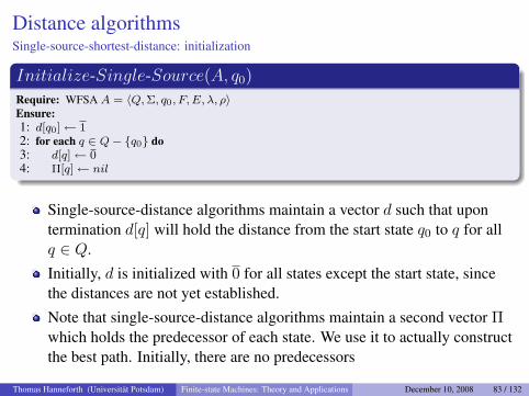
Initialize-Single-Source(A, q0)

Require: WFSA A = 〈Q,Σ, q0, F, E, λ, ρ〉Ensure:1: d[q0]← 12: for each q ∈ Q− {q0} do3: d[q]← 04: Π[q]← nil

Single-source-distance algorithms maintain a vector d such that upontermination d[q] will hold the distance from the start state q0 to q for allq ∈ Q.

Initially, d is initialized with 0 for all states except the start state, sincethe distances are not yet established.

Note that single-source-distance algorithms maintain a second vector Πwhich holds the predecessor of each state. We use it to actually constructthe best path. Initially, there are no predecessors


Distance algorithmsSingle-source-shortest-distance: Relaxation

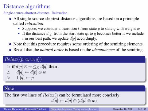
All single-source-shortest-distance algorithms are based on a principlecalled relaxation:

I Suppose, we consider a transition t from state p to state q with weight wI If the distance d[q] from the start state q0 to q becomes better if we includet in our best path, we update d[q] accordingly.

Note that this procedure requires some ordering of the semiring elements.Recall that the natural order is based on the idempotence of the semiring.

Relax(〈p, a, w, q〉)1: if d[p]⊗ w ≤K d[q] then2: d[q]← d[p]⊗ w3: Π[q]← p

NoteThe first two lines of Relax() can be formulated more concisely:

d[q]← d[q]⊕ (d[p]⊗ w)


Distance algorithmsSingle-source-shortest-distance: path properties

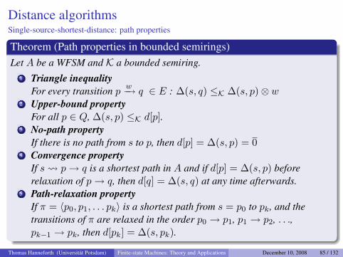
Theorem (Path properties in bounded semirings)Let A be a WFSM and K a bounded semiring.

1 Triangle inequalityFor every transition p w−→ q ∈ E : ∆(s, q) ≤K ∆(s, p)⊗ w

2 Upper-bound propertyFor all p ∈ Q, ∆(s, p) ≤K d[p].

3 No-path propertyIf there is no path from s to p, then d[p] = ∆(s, p) = 0

4 Convergence propertyIf s p→ q is a shortest path in A and if d[p] = ∆(s, p) beforerelaxation of p→ q, then d[q] = ∆(s, q) at any time afterwards.

5 Path-relaxation propertyIf π = 〈p0, p1, . . . pk〉 is a shortest path from s = p0 to pk, and thetransitions of π are relaxed in the order p0 → p1, p1 → p2, . . .,pk−1 → pk, then d[pk] = ∆(s, pk).


Distance algorithmsDAG-Distance: topological sort

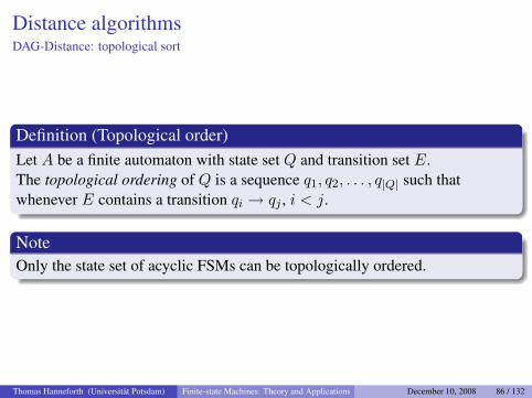
Definition (Topological order)Let A be a finite automaton with state set Q and transition set E.The topological ordering of Q is a sequence q1, q2, . . . , q|Q| such thatwhenever E contains a transition qi → qj , i < j.

NoteOnly the state set of acyclic FSMs can be topologically ordered.


Distance algorithmsDAG-Distance: topological sort

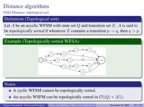
Definition (Topological sort)Let A be an acyclic WFSM with state set Q and transition set E. A is said tobe topologically sorted if whenever E contains a transition p→ q, then q > p.

Example (Topologically sorted WFSA)

�

��

��

�

��

��

��

��

��

��

��

��

��

��

��

��

��

��

��

NotesA cyclic WFSM cannot be topologically sorted.

An acyclic WSFM can be topologically sorted in O(|Q|+ |E|).


Distance algorithmsDAG-Distance(A, d)

DAG-Distance(A, d)

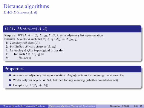
Require: WFSA A = 〈Q,Σ, q0, F, E, λ, ρ〉 in adjacency list representation.Ensure: A vector d such that ∀q ∈ Q : d[q] = ∆(q0, q)1: Topological-Sort(A)2: Initialize-Single-Source(A, q0)3: for each q ∈ Q in topological order do4: for each t ∈ Adj[q] do5: Relax(t)

PropertiesAssumes an adjacency list representation: Adj[q] contains the outgoing transitions of q.

Works only for acyclic WFSA, but then for any semiring (whether bounded or not).

Complexity: O(|Q|+ |E|).


Distance algorithmsDAG-Distance: example

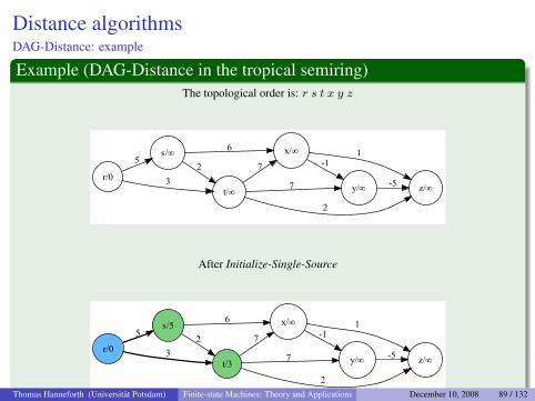
Example (DAG-Distance in the tropical semiring)The topological order is: r s t x y z

��

��

��

�

��

�

��

�

��

��

After Initialize-Single-Source

��

��

��

�

��

�

��

�

��

��

Exploring state r: d[s] and d[t] become better

��

��

��

�

��

�

��

�

�

��

Exploring state s

��

��

��

�

��

�

��

�

�

��

Exploring state t

��

��

��

�

��

�

��

�

�

��

Exploring state x: d[y] becomes better

��

��

��

�

��

�

��

�

�

��

Exploring state y: d[z] becomes better

��

��

��

�

��

�

��

�

�

��

Exploring state z

��

��

��

�

��

�

��

�

�

��

Distances after termination


Distance algorithmsDijkstra’s algorithm

Dijkstra(A, d)

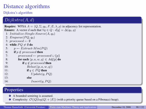
Require: WFSA A = 〈Q,Σ, q0, F, E, λ, ρ〉 in adjacency list representation.Ensure: A vector d such that ∀q ∈ Q : d[q] = ∆(q0, q)1: Initialize-Single-Source(A, q0)2: Enqueue(PQ, q0)3: processed← ∅4: while PQ 6= ∅ do5: p← Extract-Min(PQ)6: if p /∈ processed then7: processed← processed ∪ {p}8: for each 〈p, a, w, q〉 ∈ Adj[p] do9: if q /∈ processed then

10: Relax(〈p, a, w, q〉)11: if q ∈ PQ then12: Update(q, PQ)13: else14: Insert(q, PQ)

PropertiesA bounded semiring is assumed.Complexity: O(|Q|log|Q|+ |E|) (with a priority queue based on a Fibonacci heap).


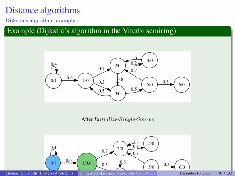
Distance algorithmsDijkstra’s algorithm: example

Example (Dijkstra’s algorithm in the Viterbi semiring)

��

��

��

��

��

��

��

��

��

��

��

��


��

��

��

��

��

��

��

��

��

��

��

��

After extracting state 0

��

��

��

��

��

��

��

��

��

��

��

��

��


��

��

��

��

��

��

��

��

��

��

��

��

��

��

��


��

��

��

��

��

��

��

��

��

��

��

��

��

��


��

��

��

��

��

��

��

��

��

��

��

��

��

��


��

��

��

��

��

��

��

��

��

��

��

��

��

��


��

��

��

��

��

��

��

��

��

��

��

��

��

��


��

��

��

��

��

��

��

��

��

��

��

��

��

��

Distances after termination


Distance algorithmsBellman-Ford algorithm

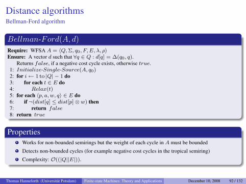
Bellman-Ford(A, d)

Require: WFSA A = 〈Q,Σ, q0, F, E, λ, ρ〉Ensure: A vector d such that ∀q ∈ Q : d[q] = ∆(q0, q).

Returns false, if a negative cost cycle exists, otherwise true.1: Initialize-Single-Source(A, q0)2: for i← 1 to |Q| − 1 do3: for each t ∈ E do4: Relax(t)5: for each 〈p, a, w, q〉 ∈ E do6: if ¬(dist[q] ≤ dist[p]⊗ w) then7: return false8: return true

PropertiesWorks for non-bounded semirings but the weight of each cycle in A must be bounded

Detects non-bounded cycles (for example negative cost cycles in the tropical semiring)

Complexity: O((|Q||E|)).


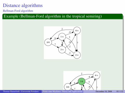
Distance algorithmsBellman-Ford algorithm

Example (Bellman-Ford algorithm in the tropical semiring)

��

��

��

��

��

��

��

�

��

�

�


��

��

��

��

��

��

��

�

��

�

�

After pass 1

��

��

��

��

��

��

�

�

�

�

�

After pass 2

��

��

��

��

��

��

�

�

�

�

�

After pass 3

��

��

��

� �

��

��

�

�

�

�

�

After pass 4

��

��

��

� �

��

��

�

�

�

�

�

After termination


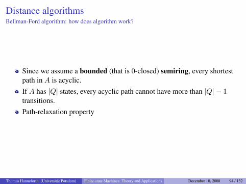
Distance algorithmsBellman-Ford algorithm: how does algorithm work?

Since we assume a bounded (that is 0-closed) semiring, every shortestpath in A is acyclic.

If A has |Q| states, every acyclic path cannot have more than |Q| − 1transitions.

Path-relaxation property


Distance algorithmsBellman-Ford algorithm: why does the negative cost cycle check work?


Distance algorithmsMohri’s algorithm for arbitrary semirings

They key idea to generalize the single-source-distance algorithms alreadyseen is, that they all are based on a certain queue discipline, that is, the statesare processed in a certain order:

DAG-distance uses a queue which contains the states in topologicalorder. Every state is processed once.

The queue in Dijkstra’s algorithm contains the states in best-first order.Every state is processed once.

The queue in Bellman-Ford’s algorithm contains the states in any order,but every state is enqueued |Q| − 1 times.



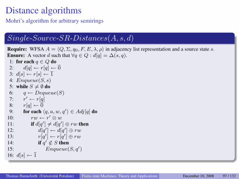
Single-Source-SR-Distances(A, s, d)

Require: WFSA A = 〈Q,Σ, q0, F, E, λ, ρ〉 in adjacency list representation and a source state s.Ensure: A vector d such that ∀q ∈ Q : d[q] = ∆(s, q).1: for each q ∈ Q do2: d[q]← r[q]← 03: d[s]← r[s]← 14: Enqueue(S, s)5: while S 6= ∅ do6: q ← Dequeue(S)7: r′ ← r[q]8: r[q]← 09: for each 〈q, a, w, q′〉 ∈ Adj[q] do

10: rw ← r′ ⊗ w11: if d[q′] 6= d[q′]⊕ rw then12: d[q′]← d[q′]⊕ rw13: r[q′]← r[q′]⊕ rw14: if q′ /∈ S then15: Enqueue(S, q′)16: d[s]← 1



NotesLines 1 to 3 initialize d[q] and r[q] for all q ∈ Q\{s} to 0.d[s] and r[q] are initialized with 1.

Lines 5 to 15 define a while loop in which a state queue is processed.The states in the queue may be processed in any order, but the queue mayalso make use of semiring properties (boundedness) or acyclicity of theWFSA.

Lines 10 to 13 define the actual relaxation step. Since we do not requirebounded semirings, the test with ≤ is replaced by 6=.


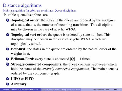
Distance algorithmsMohri’s algorithm for arbitrary semirings: Queue disciplinesPossible queue disciplines are:

1 Topological order: the states in the queue are ordered by the in-degreeof a state, that is, the number of incoming transitions. This disciplinemay be chosen in the case of acyclic WFSA.

2 Topological sort order: the queue is ordered by state number. Thisdiscipline may be chosen in the case of acyclic WFSA which aretopologically sorted.

3 Best-first: the states in the queue are ordered by the natural order of theweights in d.

4 Bellman-Ford: every state is enqueued |Q| − 1 times.5 Strongly-connected components: the queue contains subqueues which

hold the states of the strongly-connected components. The main queue isordered by the component graph.

6 LIFO or FIFO7 Arbitrary



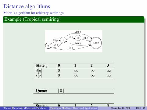
Example (Tropical semiring)

�

��

��

��

��

��

��

State q 0 1 2 3d[q] 0 ∞ ∞ ∞r[q] 0 ∞ ∞ ∞

Queue [ 0 ]

State q 0 1 2 3d[q] 0 0.2 ∞ 0.8r[q] ∞ 0.2 ∞ 0.8

Queue [ 3 1 ]

State q 0 1 2 3d[q] 0 0.2 ∞ 0.8r[q] ∞ 0.2 ∞ ∞

Queue [ 1 ]

State q 0 1 2 3d[q] 0 0.2 0.8 0.5r[q] ∞ ∞ 0.8 0.5

Queue [ 3 2 ]

State q 0 1 2 3d[q] 0 0.2 0.8 0.5r[q] ∞ ∞ 0.8 ∞

Queue [ 2 ]


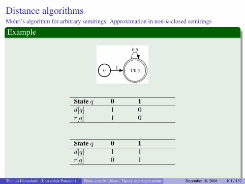
Distance algorithmsMohri’s algorithm for arbitrary semirings: Approximation in non-k-closed semirings

Example

� ��

��

State q 0 1d[q] 1 0r[q] 1 0

State q 0 1d[q] 1 1r[q] 0 1

State q 0 1d[q] 1 1.5r[q] 0 0.5

State q 0 1d[q] 1 1.75r[q] 0 0.25

State q 0 1d[q] 1 1.875r[q] 0 0.125

State q 0 1d[q] 1 1.9375r[q] 0 0.0625

State q 0 1d[q] 1 1.96875r[q] 0 0.03125

State q 0 1d[q] 1 1.984375r[q] 0 0.015625

State q 0 1d[q] 1 1.9921875r[q] 0 0.0078125

State q 0 1d[q] 1 1.9960938r[q] 0 0.00390625

State q 0 1d[q] 1 1.9980469r[q] 0 0.001953125


Distance algorithmsComputing best paths

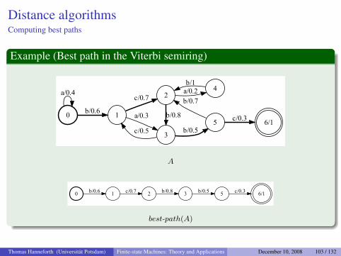
After using one of the shortest-distance algorithms, we calculate the weight ofthe best path in the following way:

Definition (Best path)

Let A = 〈Q,Σ, q0, F, E, λ, ρ〉 be a WFSA with K = 〈W,⊕,⊗, 0, 1〉 as theunderlying semiring.The weight of the best path in A is defined as follows:

best-path(A) =⊕q∈F

(λ⊗∆(q0, q)⊗ ρ(p)

)The actual best path can be reconstructed using the predecessor vector Π.

NoteNote that this corresponds to the master formula, except that the labels alongthe different paths are neglected.



Example (Best path in the Viterbi semiring)

�

��

��

�

��

��

��

��

��

��

��

��

A

� ��

��

��

��

��

best-path(A)


Distance algorithmsComputing best paths: application in morphological disambiguation

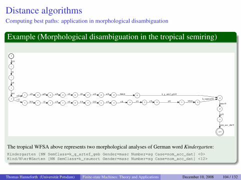
Example (Morphological disambiguation in the tropical semiring)

�

�

��

�

��

�

��

�

��

�

��

��

��

��

� ��

��

��

��

��

��

��

��

��

��

��

��

��

��

��

��

��

��

��

��

��

The tropical WFSA above represents two morphological analyses of German word Kindergarten:Kindergarten [NN SemClass=k_g_artef_geb Gender=masc Number=sg Case=nom_acc_dat] <0>Kind/N\er#Garten [NN SemClass=k_raumort Gender=masc Number=sg Case=nom_acc_dat] <12>



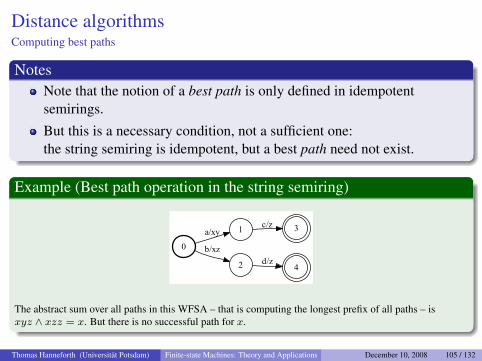
NotesNote that the notion of a best path is only defined in idempotentsemirings.

But this is a necessary condition, not a sufficient one:the string semiring is idempotent, but a best path need not exist.

Example (Best path operation in the string semiring)

�

��

�

��

��

��

The abstract sum over all paths in this WFSA – that is computing the longest prefix of all paths – isxyz ∧ xzz = x. But there is no successful path for x.


Shortest-distance algorithmsComputing n-best paths


Equivalence transformations

Equivalence transformations

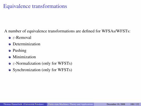
A number of equivalence transformations are defined for WFSAs/WFSTs:

ε-Removal

Determinization

Pushing

Minimization

ε-Normalization (only for WFSTs)

Synchronization (only for WFSTs)


Equivalence transformationsε-Removal

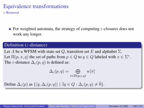
For weighted automata, the strategy of computing ε-closures does notwork any longer.

Definition (ε-distance)Let A be a WFSM with state set Q, transition set E and alphabet Σ.Let Π(p, x, q) the set of paths from p ∈ Q to q ∈ Q labeled with x ∈ Σ∗.The ε-distance ∆ε(p, q) is defined as:

∆ε(p, q) =⊕

π∈Π(p,ε,q)

w[π]

Define ∆ε(p) as {〈q,∆ε(p, q)〉 | ∃q ∈ Q : ∆ε(p, q) 6= 0}.



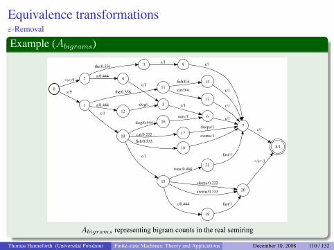
Example (Abigrams)

�

�

��

��

��

��

��

��

��

��

��

�

��

��

��

��

��

��

��

��

��

��

��

�

��

�

��

��

��

��

��

��

��

��

��

��

��

��

��

��

��

��

��

��

Abigrams representing bigram counts in the real semiring



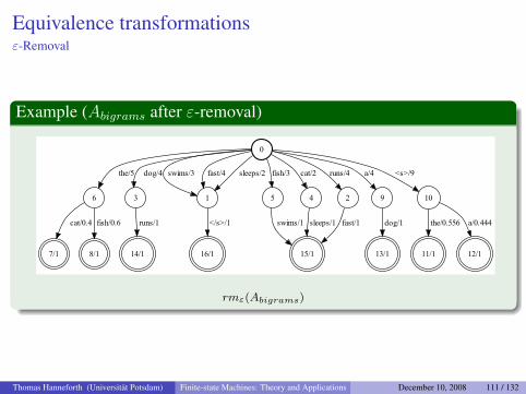
Example (Abigrams after ε-removal)

�

�

��

�

��

��

�

��

�

��

�

��

�

��

�

��

��

��

�

��

��

��

��

��

��

��

��

��

�

��

��

��

rmε(Abigrams)


Equivalence transformationsε-removal algorithm

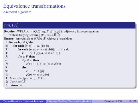
rmε(A)

Require: WFSA A = 〈Q,Σ, q0, F, E, λ, ρ〉 in adjacency list representationwith underlying semiring 〈W,⊕,⊗, 0, 1〉.

Ensure: An equivalent WFSA A′ without ε-transitions1: for each p ∈ Q do2: for each 〈q, w〉 ∈ ∆ε(p) do3: for each 〈q, a, w′, r〉 ∈ Adj[q], a 6= ε do4: E ← E ∪ {〈p, a, w ⊗ w′, r〉}5: if q ∈ F then6: if p ∈ F then7: ρ(p)← ρ(p)⊕ (w ⊗ ρ(q))8: else9: F ← F ∪ {p}

10: ρ(p)← w ⊗ ρ(q)11: E ← E\{〈p, ε, w, q〉 ∈ E}12: Connect(A)13: return A


Equivalence transformationsε-removal scheme

�

��

��

��

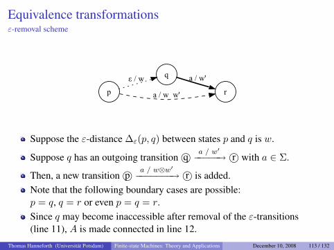
Suppose the ε-distance ∆ε(p, q) between states p and q is w.

Suppose q has an outgoing transition q© a / w′−−−−−→ r© with a ∈ Σ.

Then, a new transition p© a / w⊗w′−−−−−−−→ r© is added.Note that the following boundary cases are possible:p = q, q = r or even p = q = r.Since q may become inaccessible after removal of the ε-transitions(line 11), A is made connected in line 12.


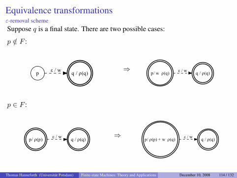
Equivalence transformationsε-removal schemeSuppose q is a final state. There are two possible cases:

p /∈ F :

� �� ⇒

��

p ∈ F :

�� ⇒

��


Equivalence transformationsε-removal algorithm: complexity


Equivalence transformationsWeighted determinization

Determinization of weighted FSAs and FSTs is based on an extension ofthe classical power set construction.

States in deterministic finite-state machines are constructed as sets ofpairs 〈q, w〉 such that q is a state of the input WFSM and w is a weight,the so called delayed weight.

The underlying semiring is required to be weakly left divisible becausewe try to realize “safe” weights as early as possible.


Equivalence transformationsWeighted determinization: algorithm

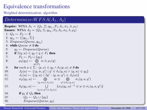
Determinize-WFSA(A1, A2)

Require: WFSA A1 = 〈Q1,Σ, q01 , F1, δ1, σ1, λ, ρ1〉Ensure: WFSA A2 = 〈Q2,Σ, q02 , F2, δ2, σ2, λ, ρ2〉1: Q2 ← F2 ← ∅2: q02 ← {〈q01 , 1〉}3: Enqueue(Queue, q02 )4: while Queue 6= ∅ do5: q2 ← Dequeue(Queue)6: if ∃〈q, w〉 ∈ q2 ∧ q ∈ F1 then7: F2 ← F2 ∪ {q2}8: ρ2(q2)←

⊕q∈F1

w ⊗ ρ1(q)

9: for each a ∈ Σ : 〈p, x〉 ∈ q2 ∧ δ1(p, a) 6= ∅ do10: J2(a)← {〈q, w, q′〉 | q′ ∈ δ1(q, a) ∧ 〈q, w〉 ∈ q2}11: J1(a)← {〈q, w〉 | ∃q′ : 〈q, w, q′〉 ∈ J2(a)}12: σ2(q2, a)←

⊕〈q,w〉∈J1(a)

w ⊗⊕

q′∈δ1(q,a)

σ1(q, a, q′)

13: δ2(q2, a)←⋃

〈q,w,q′〉∈J2(a)

{σ2(q2, a)−1 ⊗ w ⊗ σ1(q, a, q′)}

14: if q2 /∈ Q2 then15: Q2 ← Q2 ∪ {q2}16: Enqueue(Queue, q2)


Equivalence transformationsWeighted determinization: algorithm

NotesLine 3 enqueues the start state q02 of the deterministic WFSA

Lines 4 to 16 create new states



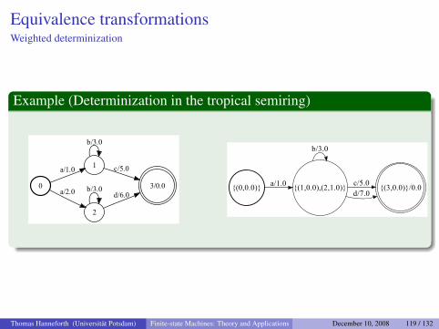
Example (Determinization in the tropical semiring)

�

��

�

��

��

��

��

��

��

��

��

��



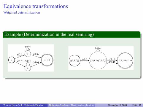
Example (Determinization in the real semiring)

�

��

�

��

��

��

��

��

��

��

��

��


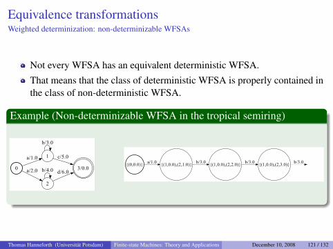
Equivalence transformationsWeighted determinization: non-determinizable WFSAs

Not every WFSA has an equivalent deterministic WFSA.

That means that the class of deterministic WFSA is properly contained inthe class of non-deterministic WFSA.

Example (Non-determinizable WFSA in the tropical semiring)

�

��

�

��

��

��

��

��

��

��

��


Equivalence transformationsWeighted determinization: non-determinizable WFSAs

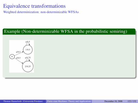
Example (Non-determinizable WFSA in the probabilistic semiring)

�

��

��

��

��

��


Equivalence transformationsWeighted determinization: twins property


Equivalence transformationsWeight Pushing

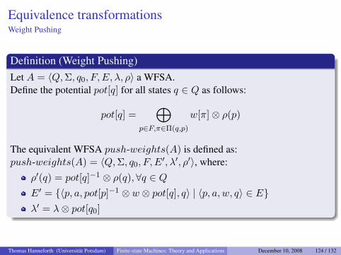
Definition (Weight Pushing)Let A = 〈Q,Σ, q0, F, E, λ, ρ〉 a WFSA.Define the potential pot[q] for all states q ∈ Q as follows:

pot[q] =⊕

p∈F,π∈Π(q,p)

w[π]⊗ ρ(p)

The equivalent WFSA push-weights(A) is defined as:push-weights(A) = 〈Q,Σ, q0, F, E

′, λ′, ρ′〉, where:

ρ′(q) = pot[q]−1 ⊗ ρ(q),∀q ∈ QE′ = {〈p, a, pot[p]−1 ⊗ w ⊗ pot[q], q〉 | 〈p, a, w, q〉 ∈ E}λ′ = λ⊗ pot[q0]



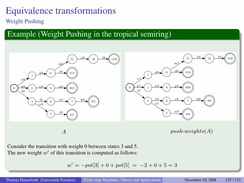
Example (Weight Pushing in the tropical semiring)

�

�

��

��

�

��

��

��

��

��

��

��

��

��

��

��

��

��

A

�

�

��

��

�

��

��

��

��

��

��

��

��

��

��

��

��

��

push-weights(A)

Consider the transition with weight 0 between states 3 and 5.The new weight w′ of this transition is computed as follows:

w′ = −pot[3] + 0 + pot[5] = −2 + 0 + 5 = 3



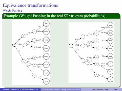
Example (Weight Pushing in the real SR: trigram probabilities)

�

�

��

��

�

��

��

��

��

��

��

��

�

��

��

��

��

��

��

��

��

��

��

��

��

�

�

��

��

�

��

��

��

��

��

��

�

��

��

��

��

� ��

��

��

��

��

��

��

��

��



Weight pushing is always possible, regardless whether the input WFSAis deterministic or not.In case of deterministic WFSA, weight pushing leads to a canonical ornormal form of the input WFSA A:

I For every x ∈ Σ∗ there is at most a single path in A.I On that path, the path weight is pushed as much as possible towards the

start state.


Equivalence transformationsWeighted minimization

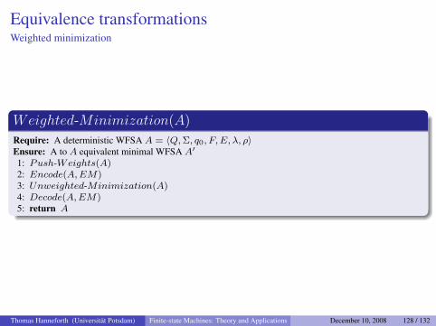
Weighted-Minimization(A)

Require: A deterministic WFSA A = 〈Q,Σ, q0, F, E, λ, ρ〉Ensure: A to A equivalent minimal WFSA A′

1: Push-Weights(A)2: Encode(A,EM)3: Unweighted-Minimization(A)4: Decode(A,EM)5: return A


Equivalence transformationsWeighted minimization

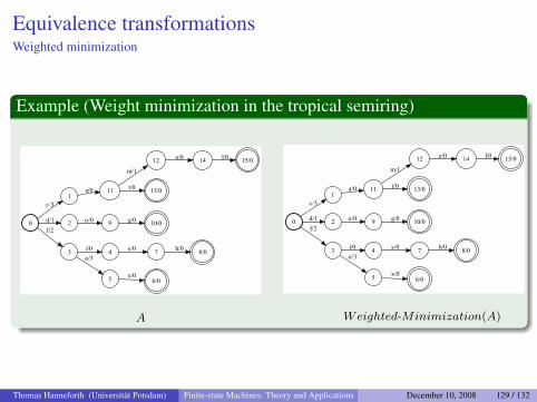
Example (Weight minimization in the tropical semiring)

�

�

��

��

�

��

��

��

��

��

��

��

��

��

��

��

��

��

A

�

�

��

��

�

��

��

��

��

��

��

��

��

��

��

��

��

��

Weighted-Minimization(A)


Outline

6 Literature


Literature


Versions

31.10.2008: version 0.1 (initial version)

14.11.2008: version 0.2 (added shortest-distance algorithms)

23.11.2008: version 0.3 (changed Dijkstra algorithm, added shortest pathproperties, added ε-filter example)

1.12.2008: version 0.4 (added equivalence transformation section)


Documents

Finite-state Machines: Theory and Applications - Weighted ... · Finite-state Machines: Theory and Applications Weighted Finite-state Automata Thomas Hanneforth Institut f¨ur Linguistik