Embed Size (px)
Citation preview
Finite-State Verification or Model Checking
Finite State Verification (FSV) or ModelChecking• Holds the promise of providing a cost effective way
of verifying important properties about a system• Not all faults are created equal• Invest effort into most important properties
• Several promising prototypes• Reachability Based
• SPIN• Symbolic Model Checking (SMV)• LTSA
• Flow Equations• Integer Necessary Conditions (INCA)
• Data Flow Analysis• FLAVERS
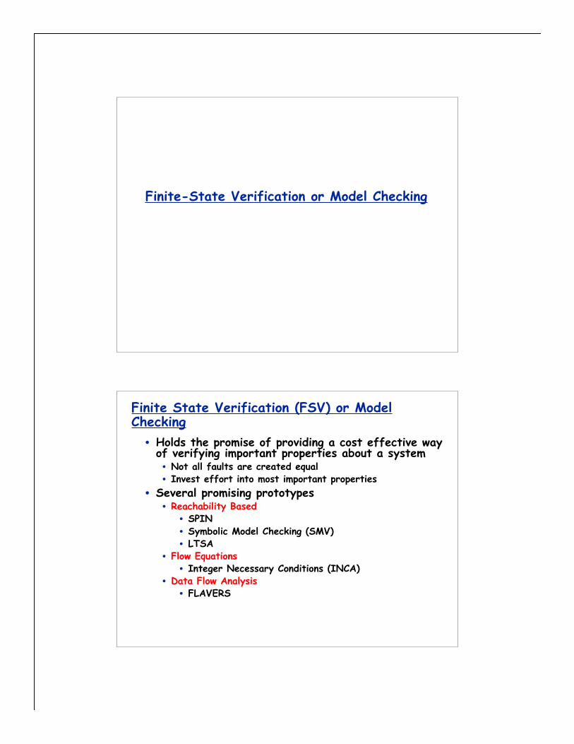
Property
System
Property Translator
SystemTranslator
ReasoningEngine
System Model Property Verified
PropertyRepresentation
Counter Examplesfor Model
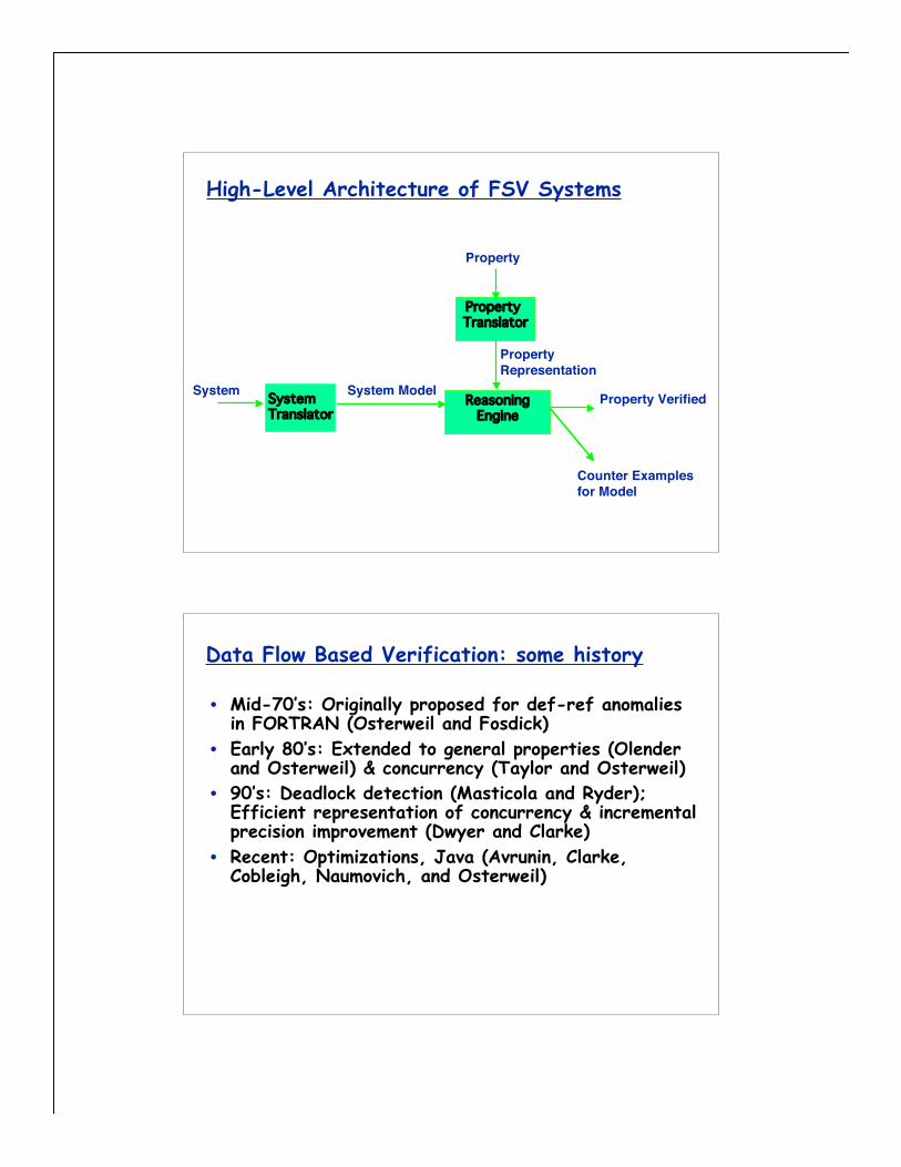
High-Level Architecture of FSV Systems
Conservative Analysis
• If property verified, property holds for allpossible executions of the system
• If property not verified:• An error found (in the system or in theproperty)
OR
• A spurious result• System model abstracts information to betractable
• Conservative abstractions usually over-approximate behavior
• If inconsistency relies upon over-approximations, then a spurious result• e.g. every counterexample corresponds to an infeasiblepath
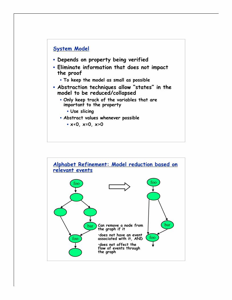
System Model
• Depends on property being verified• Eliminate information that does not impactthe proof• To keep the model as small as possible
• Abstraction techniques allow “states” in themodel to be reduced/collapsed• Only keep track of the variables that areimportant to the property• Use slicing
• Abstract values whenever possible• x<0, x=0, x>0
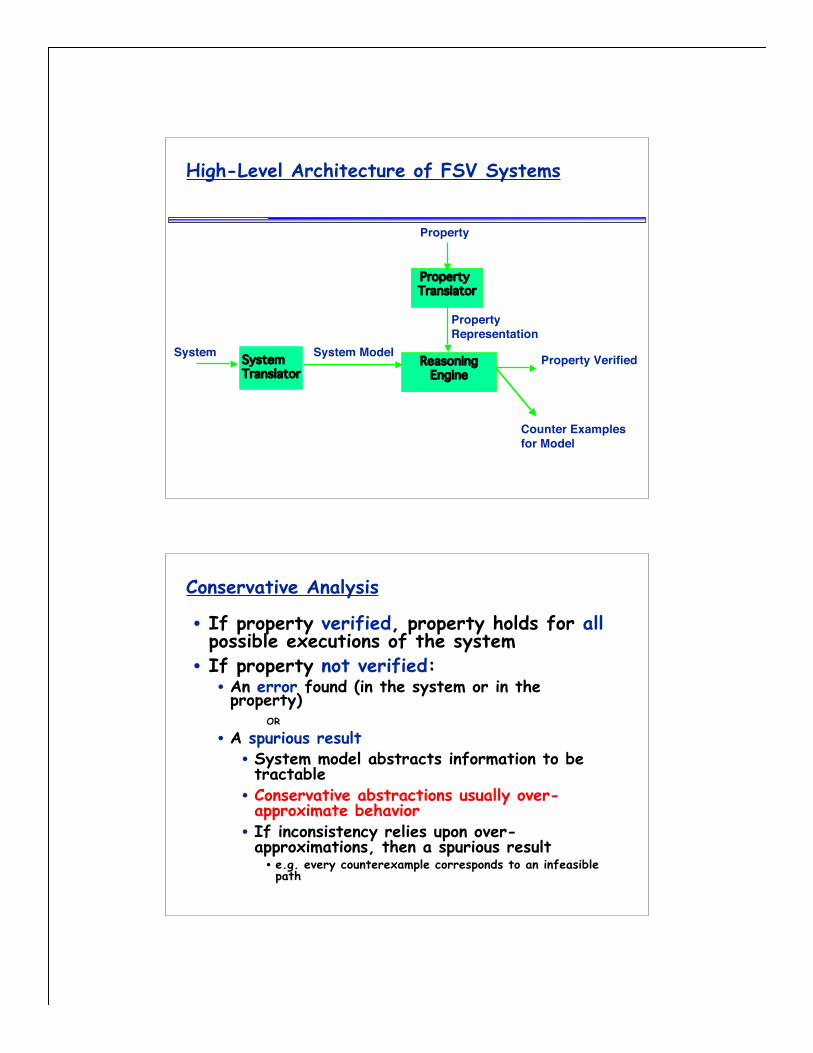
Alphabet Refinement: Model reduction based onrelevant events
foo
foo
bar
foo
foo
barCan remove a node fromthe graph if it•does not have an eventassociated with it, AND•does not affect theflow of events throughthe graph
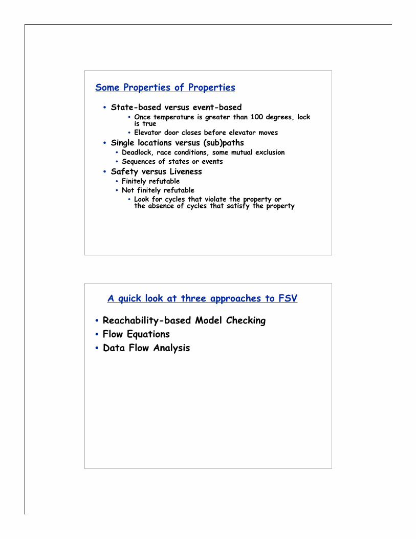
Some Properties of Properties
• State-based versus event-based• Once temperature is greater than 100 degrees, lock
is true• Elevator door closes before elevator moves
• Single locations versus (sub)paths• Deadlock, race conditions, some mutual exclusion• Sequences of states or events
• Safety versus Liveness• Finitely refutable• Not finitely refutable
• Look for cycles that violate the property orthe absence of cycles that satisfy the property
A quick look at three approaches to FSV
• Reachability-based Model Checking• Flow Equations• Data Flow Analysis
Reachability-based Model Checking: somehistory• Originally proposed for hardware• Early 80’s: E. Clarke and Emerson;
Quielle and Sifakis• Late 80’s: Improved algorithms and property
notations (E. Clarke, Emerson, Sistla)• 90’s: Symbolic Model Checking (SMV) and other
optimizations (Burch, E. Clarke, Dill, Long, andMcMillan)
• Current: Hybrid approaches that combine modelchecking with• Theorem proving techniques• Symbolic execution• Optimization techniques (e.g., points to analysis)
Model Checking: Overview
• Properties usually expressed in a temporallogic
• System represented as a (possibly“abstracted”) reachability graph• State based=>show the values of all the “relevant”variables
• Reasoning engine propagates valid subformulasthrough the graph
Temporal Logic Property
System
Property Translator
SystemTranslator
Subformula propagation
State-based Reachability
Graph Property Verified
PropertyRepresentation
Counter Examplesfor Model
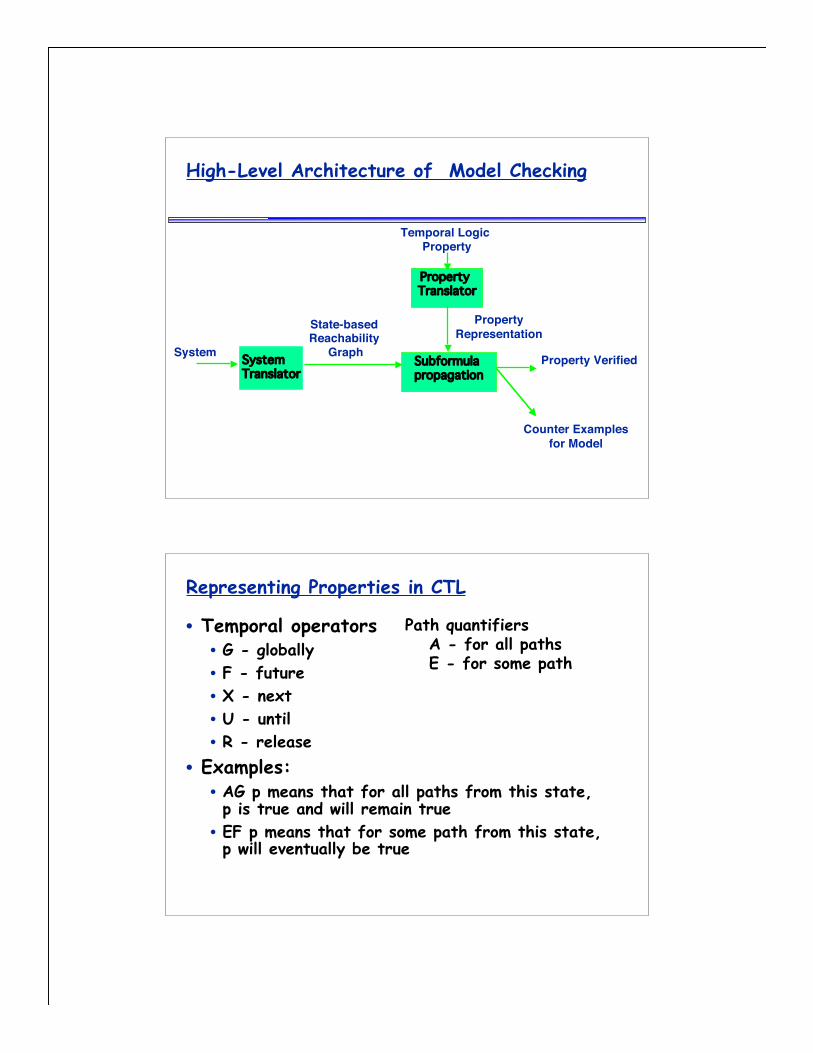
High-Level Architecture of Model Checking
Representing Properties in CTL
• Temporal operators• G - globally• F - future• X - next• U - until• R - release
• Examples:• AG p means that for all paths from this state,p is true and will remain true
• EF p means that for some path from this state,p will eventually be true
Path quantifiersA - for all pathsE - for some path

Assigning propositions to nodes
• Mark nodes with propositions that are true atthat node
• Each type of expression has a rule for how topropagate that expression through the graph• E.g., Mark a node with AXp (EXp) if for all(some) of its successors p is true
Propagating Propositions: AXp and EXp
p
p
p
X p - in the next state, p is true
p
p
EX pAX p
Consider AX p Consider EX p
Only need to look at the successors of the node of interest
EX p
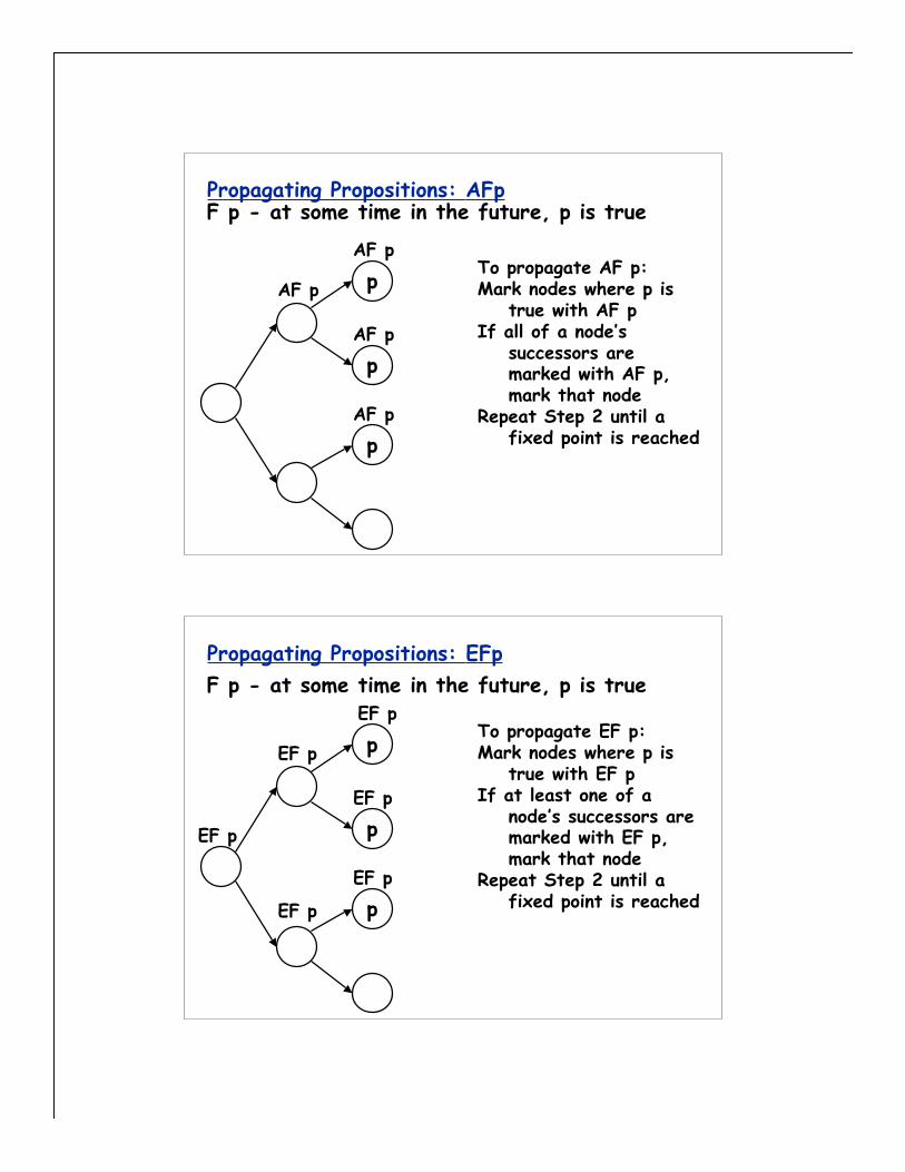
Propagating Propositions: AFp
p
p
p
F p - at some time in the future, p is true
AF p
AF p
AF p
AF pTo propagate AF p:Mark nodes where p is
true with AF pIf all of a node’s
successors aremarked with AF p,mark that node
Repeat Step 2 until afixed point is reached
Propagating Propositions: EFpF p - at some time in the future, p is true
EF p
EF p
EF p
EF p
EF p
EF p
p
p
p
To propagate EF p:Mark nodes where p is
true with EF pIf at least one of a
node’s successors aremarked with EF p,mark that node
Repeat Step 2 until afixed point is reached
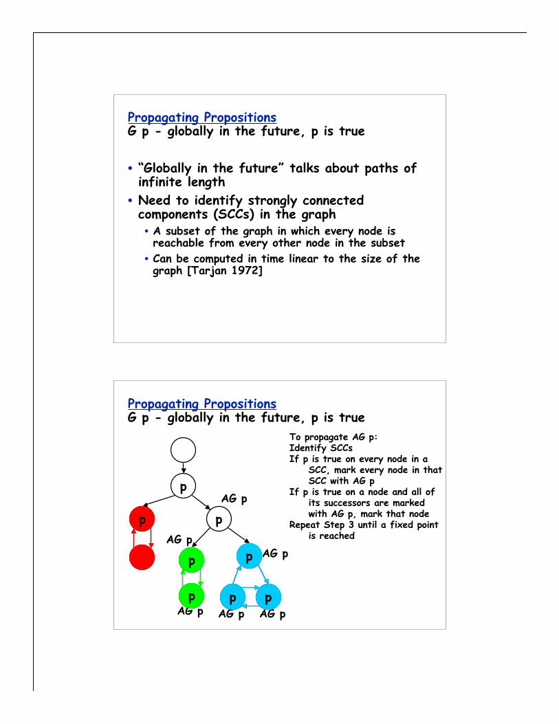
Propagating PropositionsG p - globally in the future, p is true
• “Globally in the future” talks about paths ofinfinite length
• Need to identify strongly connectedcomponents (SCCs) in the graph• A subset of the graph in which every node isreachable from every other node in the subset
• Can be computed in time linear to the size of thegraph [Tarjan 1972]
Propagating PropositionsG p - globally in the future, p is true
p
pp
ppp
p
p
To propagate AG p:Identify SCCsIf p is true on every node in a
SCC, mark every node in thatSCC with AG p
If p is true on a node and all ofits successors are markedwith AG p, mark that node
Repeat Step 3 until a fixed pointis reached
AG p
AG p
AG pAG p
AG p
AG p
p
p
p
p
pp
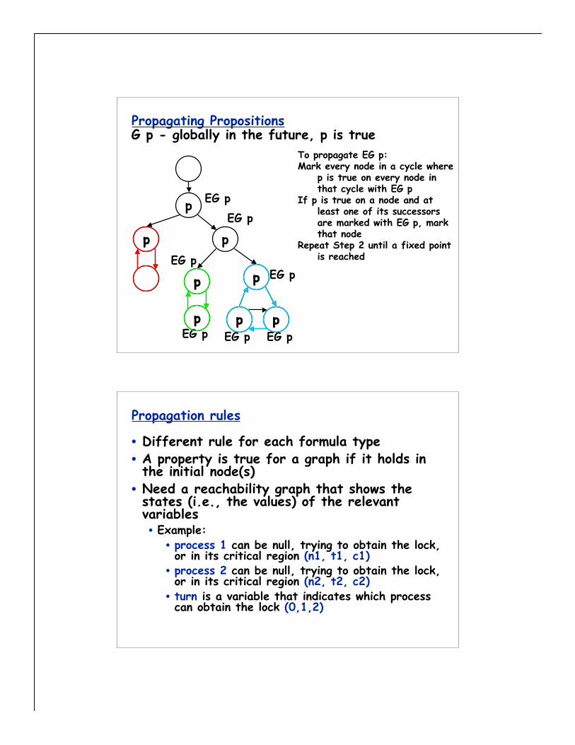
Propagating PropositionsG p - globally in the future, p is true
p
p
To propagate EG p:Mark every node in a cycle where
p is true on every node inthat cycle with EG p
If p is true on a node and atleast one of its successorsare marked with EG p, markthat node
Repeat Step 2 until a fixed pointis reached
EG p
EG p
EG pEG p
EG p
EG p
EG p
pp
ppp
pp
p
p
p
pp
Propagation rules
• Different rule for each formula type• A property is true for a graph if it holds inthe initial node(s)
• Need a reachability graph that shows thestates (i.e., the values) of the relevantvariables• Example:
• process 1 can be null, trying to obtain the lock,or in its critical region (n1, t1, c1)
• process 2 can be null, trying to obtain the lock,or in its critical region (n2, t2, c2)
• turn is a variable that indicates which processcan obtain the lock (0,1,2)
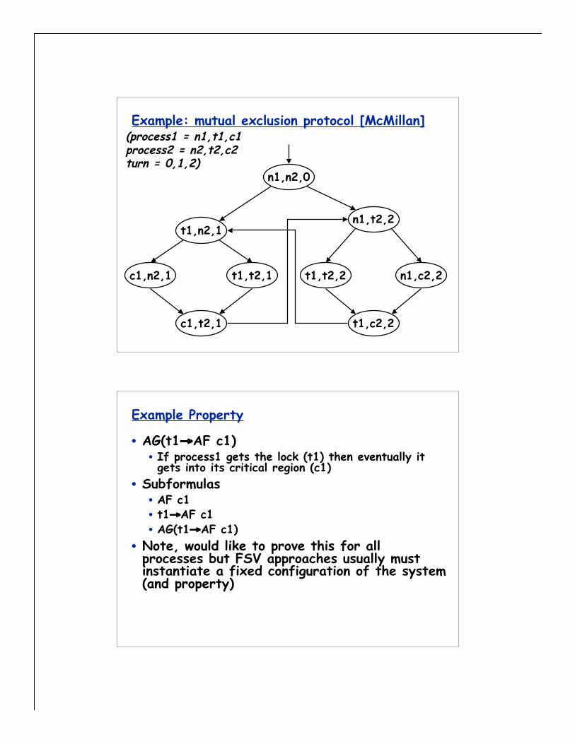
Example: mutual exclusion protocol [McMillan](process1 = n1,t1,c1process2 = n2,t2,c2turn = 0,1,2)
n1,n2,0
t1,n2,1n1,t2,2
n1,c2,2t1,t2,2
t1,c2,2
t1,t2,1c1,n2,1
c1,t2,1
Example Property
• AG(t1→AF c1)• If process1 gets the lock (t1) then eventually itgets into its critical region (c1)
• Subformulas• AF c1• t1→AF c1• AG(t1→AF c1)
• Note, would like to prove this for allprocesses but FSV approaches usually mustinstantiate a fixed configuration of the system(and property)

Example: propagation
(process1, process2, turn)
n1,n2,0
t1,n2,1n1,t2,2
n1,c2,2t1,t2,2
t1,c2,2
t1,t2,1c1,n2,1
c1,t2,1
AG(t1→AF c1)AG(t1→AF c1)
AF c1
AF c1
AF c1
AF c1
AF c1
AF c1
AF c1
AF c1
AF c1
Need to continue propagating
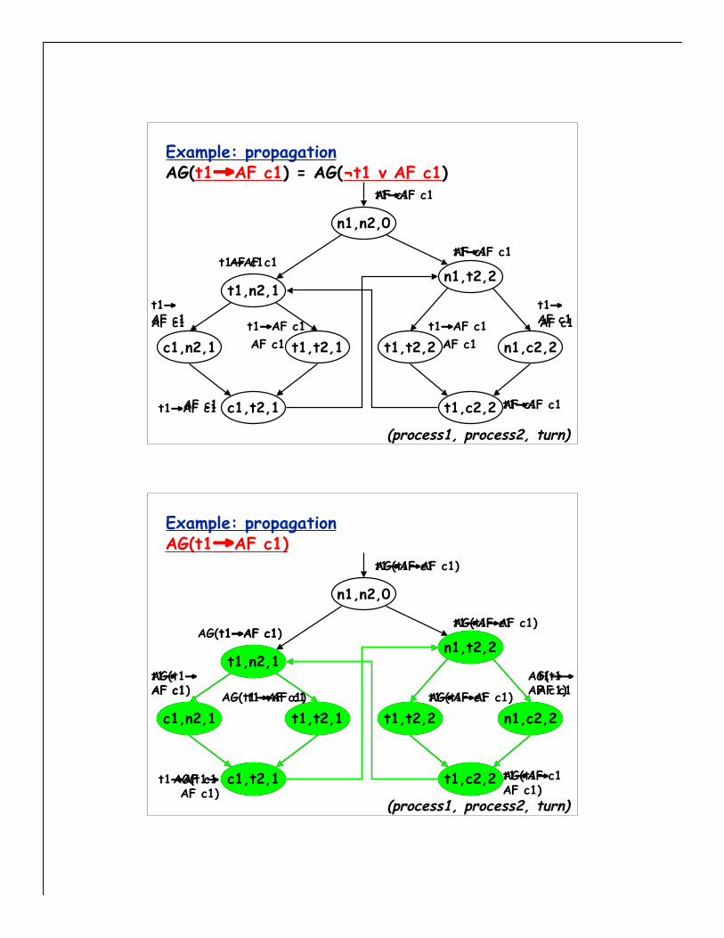
• AG(t1→AF c1)• (t1→AF c1)• equivalent to (¬t1 v AF c1)
Example: propagation
(process1, process2, turn)
n1,n2,0
t1,n2,1n1,t2,2
n1,c2,2t1,t2,2
t1,c2,2
t1,t2,1c1,n2,1
c1,t2,1AF c1
AF c1
AF c1
AF c1
AF c1
AF c1
AF c1
AF c1
AF c1AG(t1→AF c1) = AG(¬t1 v AF c1)
t1→AF c1
t1→AF c1
t1→AF c1
t1→AF c1
t1→AF c1
t1→AF c1t1→AF c1
t1→AF c1
t1→AF c1
Example: propagation
(process1, process2, turn)
n1,n2,0
t1,n2,1n1,t2,2
n1,c2,2t1,t2,2
t1,c2,2
t1,t2,1c1,n2,1
c1,t2,1
AG(t1→AF c1)
AG(t1→AF c1)
AG(t1→AF c1)
AG(t1→AF c1)
AG(t1→AF c1)
AG(t1→AF c1)
AG(t1→AF c1)AG(t1→AF c1)
AG(t1→AF c1)
t1,n2,1n1,t2,2
n1,c2,2t1,t2,2
t1,c2,2
t1,t2,1c1,n2,1
c1,t2,1t1→AF c1
t1→AF c1
t1→AF c1
t1→AF c1
t1→AF c1
t1→AF c1t1→AF c1
t1→AF c1
AG(t1→AF c1)t1→AF c1
Example: propagation
(process1, process2, turn)
n1,n2,0
t1,n2,1n1,t2,2
n1,c2,2t1,t2,2
t1,c2,2
t1,t2,1c1,n2,1
c1,t2,1AG(t1→AF c1)
AG(t1→AF c1)
AG(t1→AF c1)
AG(t1→AF c1)
AG(t1→AF c1)
AG(t1→AF c1)AG(t1→AF c1)
AG(t1→AF c1)
t1,n2,1n1,t2,2
n1,c2,2t1,t2,2
t1,c2,2
t1,t2,1c1,n2,1
c1,t2,1
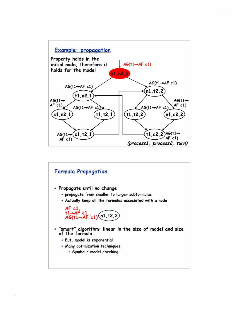
AG(t1→AF c1)Property holds in theinitial node, therefore itholds for the model
Formula Propagation
• Propagate until no change• propagate from smaller to larger subformulas• Actually keep all the formulas associated with a node
AF c1,t1→AF c1 ,AG(t1→AF c1)
• “smart” algorithm: linear in the size of model and sizeof the formula• But, model is exponential• Many optimization techniques
• Symbolic model checking
n1,t2,2
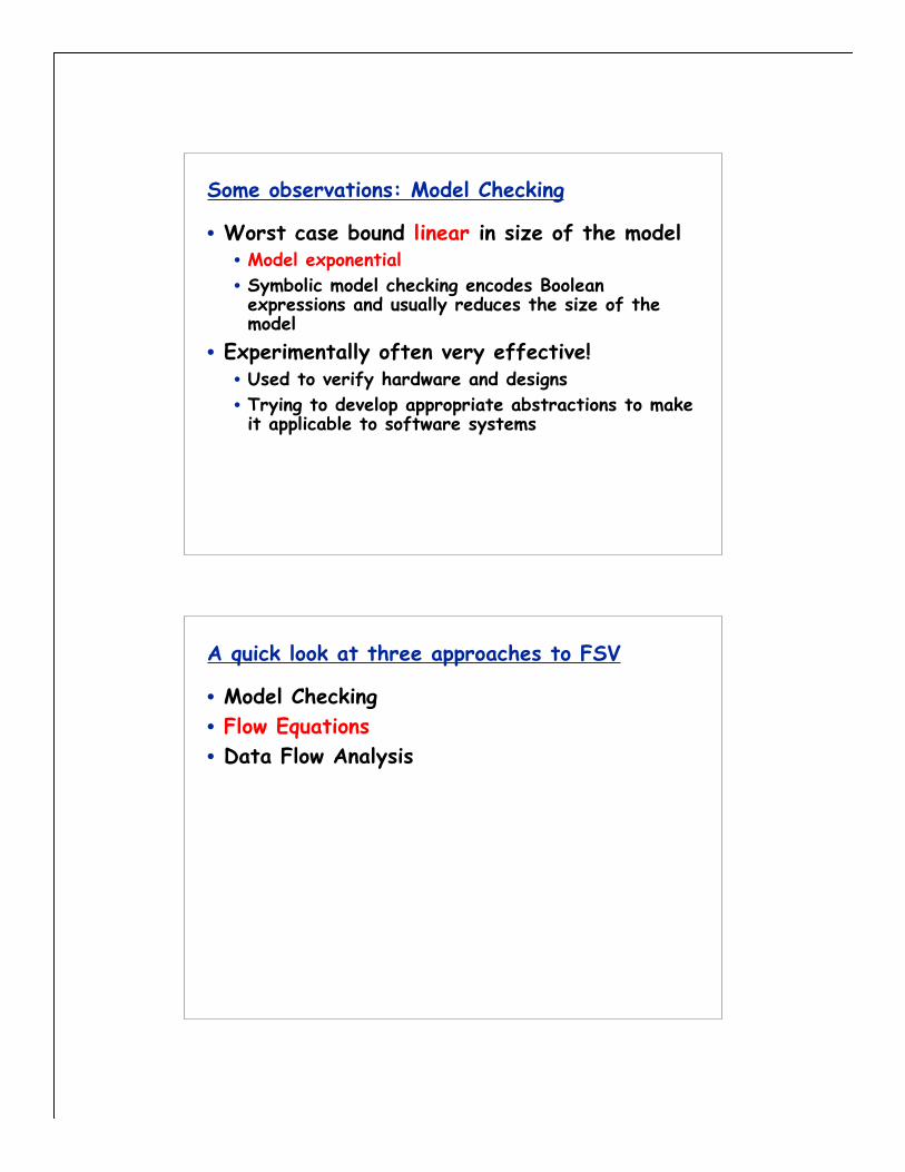
Some observations: Model Checking
• Worst case bound linear in size of the model• Model exponential• Symbolic model checking encodes Booleanexpressions and usually reduces the size of themodel
• Experimentally often very effective!• Used to verify hardware and designs• Trying to develop appropriate abstractions to makeit applicable to software systems
A quick look at three approaches to FSV
• Model Checking• Flow Equations• Data Flow Analysis

Flow Equations: some history
• Originally proposed for designs• Early 80’s: Initial development(Avrunin, Dillon, and Wileden)
• 90’s: Optimized and extended to real-time(Avrunin, Buy, Corbett, Dillon, and Wileden)
• Current: INCA prototype (Avrunin, Corbett,and Siegel)
Flow Equations
• Model system as a set of finite stateautomata
• Use extended network flow inequalitiesto capture legal flow through aconcurrent system
• Represent complement of the propertyand see if it is consistent with the setof system inequalities
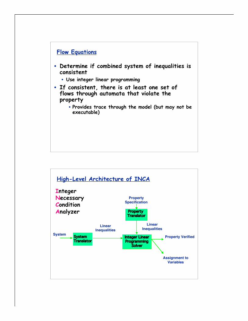
Flow Equations
• Determine if combined system of inequalities isconsistent• Use integer linear programming
• If consistent, there is at least one set offlows through automata that violate theproperty
• Provides trace through the model (but may not beexecutable)
PropertySpecification
System
Property Translator
SystemTranslator
Integer LinearProgramming
Solver
LinearInequalities
Property Verified
LinearInequalities
Assignment toVariables
High-Level Architecture of INCA
IntegerNecessaryConditionAnalyzer
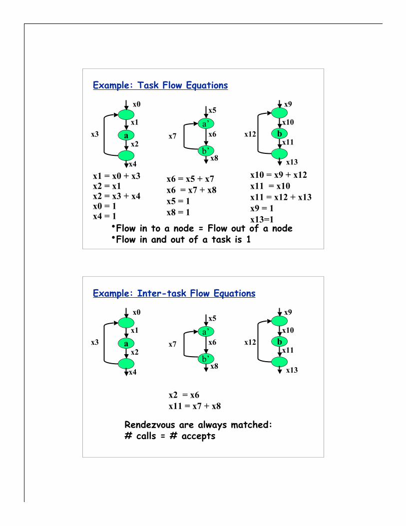
Example: Task Flow Equations
aa’
b’
b
x1 = x0 + x3x2 = x1x2 = x3 + x4x0 = 1x4 = 1
x10 = x9 + x12x11 = x10x11 = x12 + x13x9 = 1x13=1
x6 = x5 + x7x6 = x7 + x8x5 = 1x8 = 1
x1
x2x3
x5
x6x7
x10
x11x12
x0 x9
x4x8 x13
•Flow in to a node = Flow out of a node•Flow in and out of a task is 1
Example: Inter-task Flow Equations
a bx1
x2x3
x10
x11x12
x0 x9
x4 x13
x2 = x6x11 = x7 + x8
Rendezvous are always matched:# calls = # accepts
a’
b’
x5
x6x7
x8
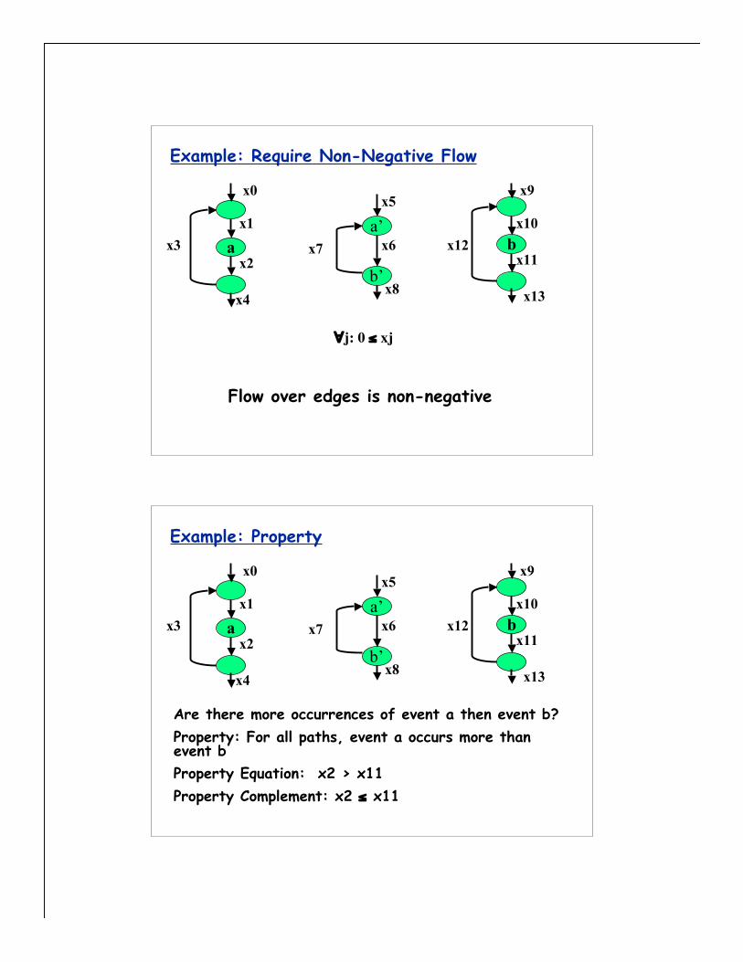
Example: Require Non-Negative Flow
a bx1
x2x3
x10
x11x12
x0 x9
x4 x13
∀j: 0 ≤ xj
Flow over edges is non-negative
a’
b’
x5
x6x7
x8
Example: Property
a bx1
x2x3
x10
x11x12
x0 x9
x4 x13
Are there more occurrences of event a then event b?Property: For all paths, event a occurs more thanevent bProperty Equation: x2 > x11Property Complement: x2 ≤ x11
a’
b’
x5
x6x7
x8
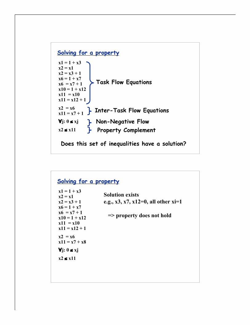
Solving for a propertyx1 = 1 + x3x2 = x1x2 = x3 + 1x6 = 1 + x7x6 = x7 + 1x10 = 1 + x12x11 = x10x11 = x12 + 1
x2 = x6x11 = x7 + 1∀j: 0 ≤ xjx2 ≤ x11
Task Flow Equations
Inter-Task Flow Equations
Non-Negative FlowProperty Complement
Does this set of inequalities have a solution?
Solving for a propertyx1 = 1 + x3x2 = x1x2 = x3 + 1x6 = 1 + x7x6 = x7 + 1x10 = 1 + x12x11 = x10x11 = x12 + 1
x2 = x6x11 = x7 + x8∀j: 0 ≤ xjx2 ≤ x11
Solution existse.g., x3, x7, x12=0, all other xi=1
=> property does not hold
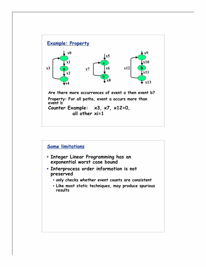
Example: Property
a bx1
x2x3
x10
x11x12
x0 x9
x4 x13
Are there more occurrences of event a then event b?Property: For all paths, event a occurs more thanevent bCounter Example: x3, x7, x12=0,
all other xi=1
a’
b’
x5
x6x7
x8
Some limitations
• Integer Linear Programming has anexponential worst case bound
• Interprocess order information is notpreserved• only checks whether event counts are consistent• Like most static techniques, may produce spuriousresults

Benefits of the approach
• Does not enumerate the state space!• ILP is often very efficient
• Empirical evidence: linear inequality systemsusually grow linearly and take sub-exponentialtimes to solve
• In practice, INCA is often an effectivetechnique
A quick look at three approaches to FSV
• Reachability-based Model Checking• Flow Equations• Data Flow Analysis
• FLAVERS
Property
System
Property Translator
SystemTranslator
ReasoningEngine
System Model Property Verified
PropertyRepresentation
Counter Examplesfor Model
High-Level Architecture of FSV Systems
Data Flow Based Verification: some history
• Mid-70’s: Originally proposed for def-ref anomaliesin FORTRAN (Osterweil and Fosdick)
• Early 80’s: Extended to general properties (Olenderand Osterweil) & concurrency (Taylor and Osterweil)
• 90’s: Deadlock detection (Masticola and Ryder);Efficient representation of concurrency & incrementalprecision improvement (Dwyer and Clarke)
• Recent: Optimizations, Java (Avrunin, Clarke,Cobleigh, Naumovich, and Osterweil)
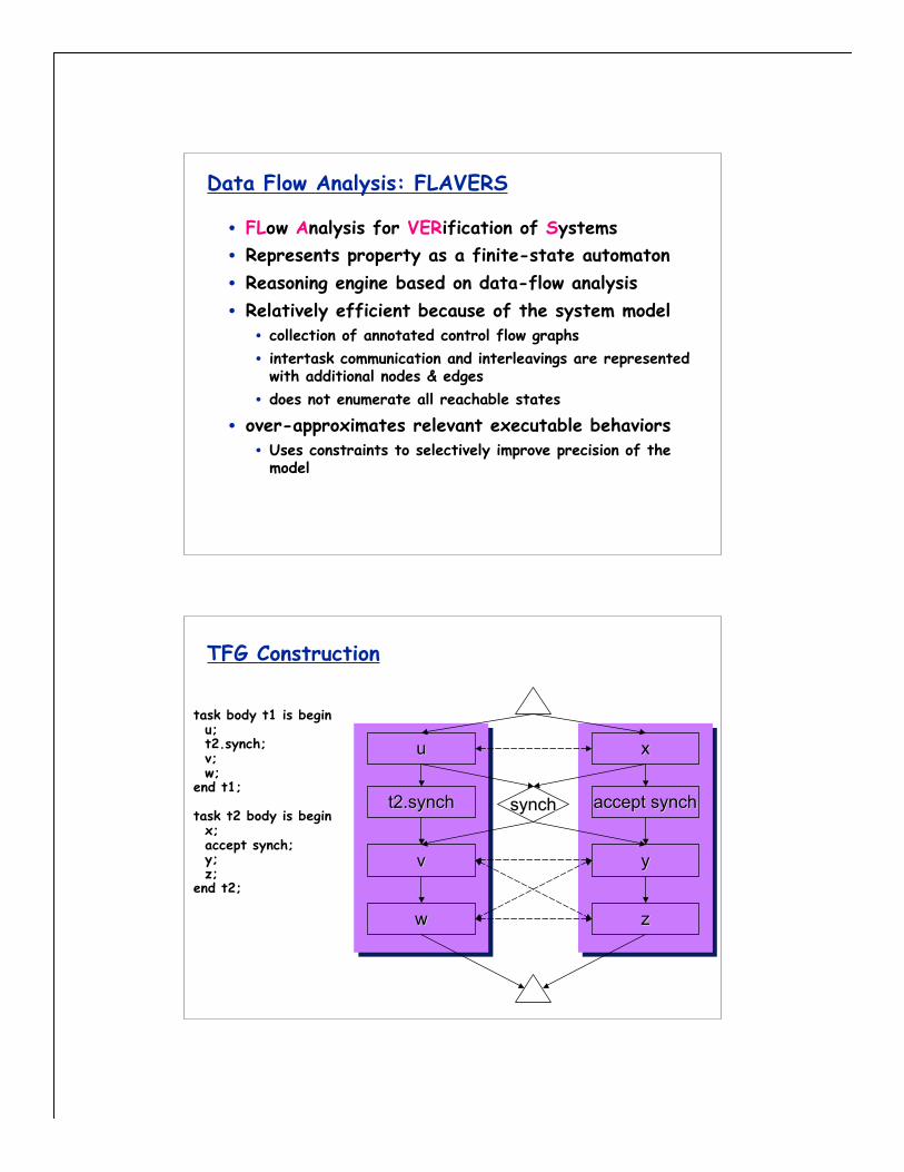
Data Flow Analysis: FLAVERS
• FLow Analysis for VERification of Systems• Represents property as a finite-state automaton• Reasoning engine based on data-flow analysis• Relatively efficient because of the system model
• collection of annotated control flow graphs• intertask communication and interleavings are represented
with additional nodes & edges• does not enumerate all reachable states
• over-approximates relevant executable behaviors• Uses constraints to selectively improve precision of the
model
`̀`̀
TFG Construction
xx
yy
uu
vv
ww
synchsynch accept synchaccept syncht2.syncht2.synch
task body t1 is begin u; t2.synch; v; w;end t1;
task t2 body is begin x; accept synch; y; z;end t2;
zz
xx
yy
uu
vv
ww
synchsynch
zz
bb,,bb
u,u,bb
u,xu,x
bb,x,x
ss,,ss
ss,y,yv,v,ss
w,w,ss v,yv,y
w,yw,y
ee,,ee
ss,z,z
v,zv,z
w,zw,z
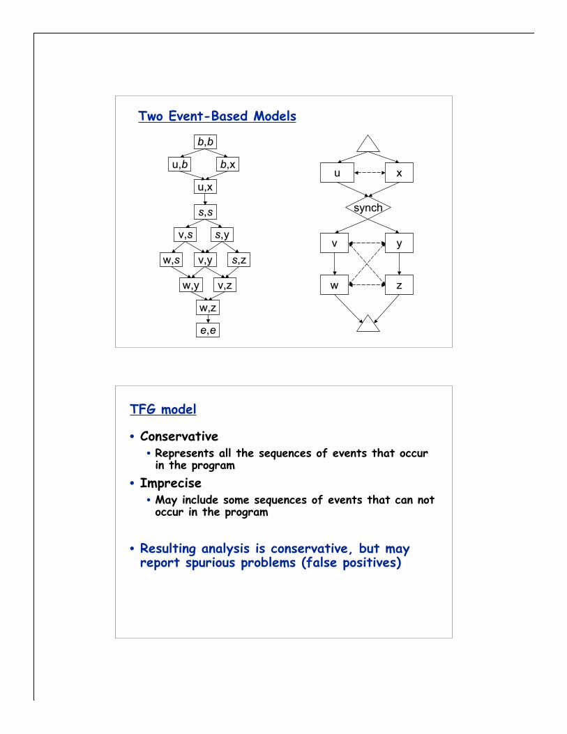
Two Event-Based Models
TFG model
• Conservative• Represents all the sequences of events that occurin the program
• Imprecise• May include some sequences of events that can notoccur in the program
• Resulting analysis is conservative, but mayreport spurious problems (false positives)

PropertySpecification
System
Property Translator
SystemTranslator
StatePropagation
Trace Flow Graph(TFG)
Property Verified
Property FSA
Counter ExampleTrace through TFG
High-Level Architecture of FLAVERS
FLAVERS
• Forward Flow, Any Path Problem• IN and OUT are sets of FSA states• IN(n) = ∪ OUT(m)
• OUT(n) = ∪ δ(s, n)
• δ is the FSA transition function• Result: Let f be the final node of the TFG
• All property: Want OUT(f) ⊆ Accept(P)• None property: Want OUT(f) ∩ Accept(P) = ∅• Accept(P) is the set of accepting states of a property, P
• Similar to Cesar, but state propagation being appliedto a Trace Flow Graph
m inpred(n)
s in IN(n)
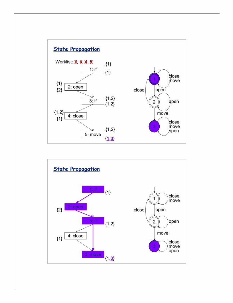
State Propagation
1
22
3
closeclose openopen
movemove
closeclosemovemoveopenopen
openopen
closeclosemovemove
WorklistWorklist: 2, 3: 2, 3
{1}{1}
{2}{2}
{1}{1}
{1,2}{1,2}
{{11,,33}}
, 4, 5, 4, 5
2: open2: open
4: close4: close
5: move5: move
3: if3: if
1: if1: if{1}{1}
{1}{1}
{1,2}{1,2}
{1,2}{1,2}
{1,2}{1,2}
State Propagation
1: if
2: open
3: if
4: close4: close
5: move
{1}{1}
{2}{2}
{1}{1}
{1,2}{1,2}
{1,{1,33}}
11
22
3
closeclose openopen
movemove
closeclosemovemoveopenopen
openopen
closeclosemovemove

State Propagation
1: if
2: open
3: if
4: close4: close
5: move
……1:1: if (stopped) thenif (stopped) then2:2: open;open;
end if;end if;……
3:3: if (stopped) thenif (stopped) then4:4: close;close;
end if;end if;……
5:5: move;move;……
PropertySpecification
System
Property Translator
SystemTranslator
StatePropagation
Trace Flow GraphProperty Verified
Property FSA
Counter ExampleTrace through TFG
Incrementally Improving Precision
...
Constraints
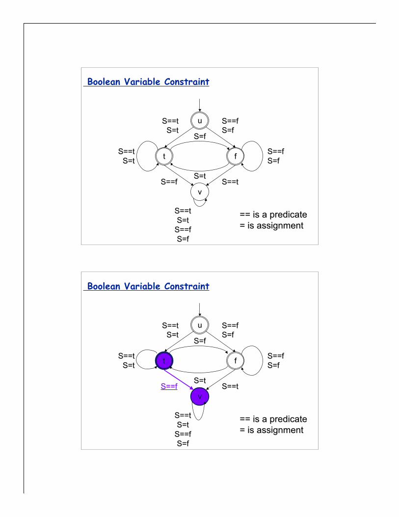
Boolean Variable Constraint
== is a predicate== is a predicate= is assignment= is assignment
S==tS==tS=tS=t
S==tS==tS=tS=t
S==tS==t
S==fS==fS=fS=f
S==fS==f
S==tS==tS=tS=t
S==fS==fS=fS=f
S==fS==fS=fS=f
S=fS=f
S=tS=t
uu
fftt
vv
Boolean Variable Constraint
== is a predicate== is a predicate= is assignment= is assignment
S==tS==tS=tS=t
S==tS==tS=tS=t
S==tS==t
S==fS==fS=fS=f
S==fS==f
S==tS==tS=tS=t
S==fS==fS=fS=f
S==fS==fS=fS=f
S=fS=f
S=tS=t
uu
fft
v
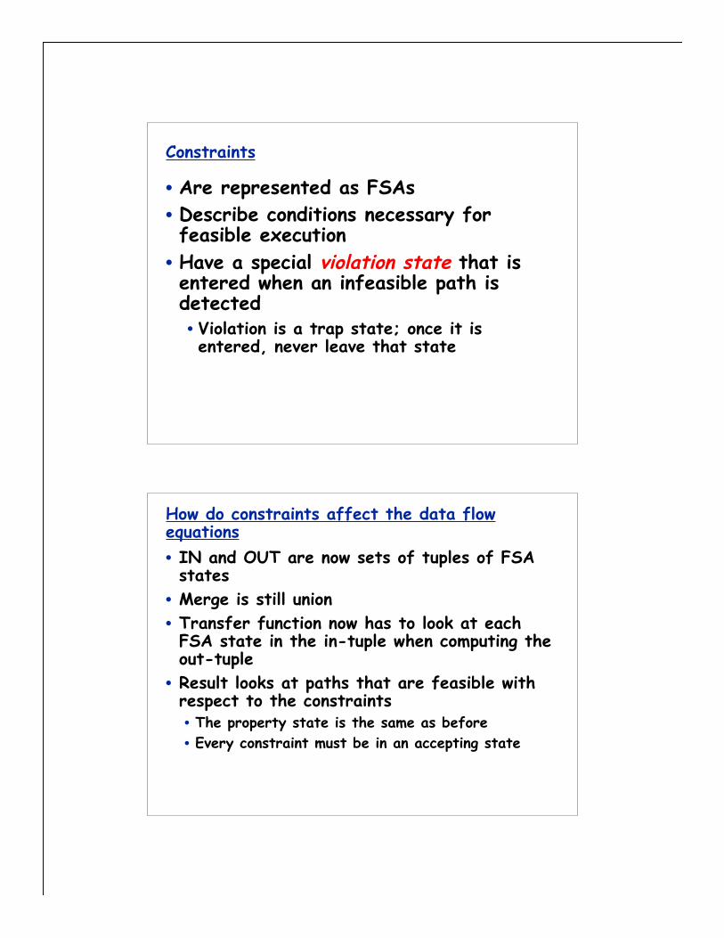
Constraints
• Are represented as FSAs• Describe conditions necessary forfeasible execution• Have a special violation state that isentered when an infeasible path isdetected• Violation is a trap state; once it isentered, never leave that state
How do constraints affect the data flowequations• IN and OUT are now sets of tuples of FSAstates
• Merge is still union• Transfer function now has to look at eachFSA state in the in-tuple when computing theout-tuple
• Result looks at paths that are feasible withrespect to the constraints• The property state is the same as before• Every constraint must be in an accepting state
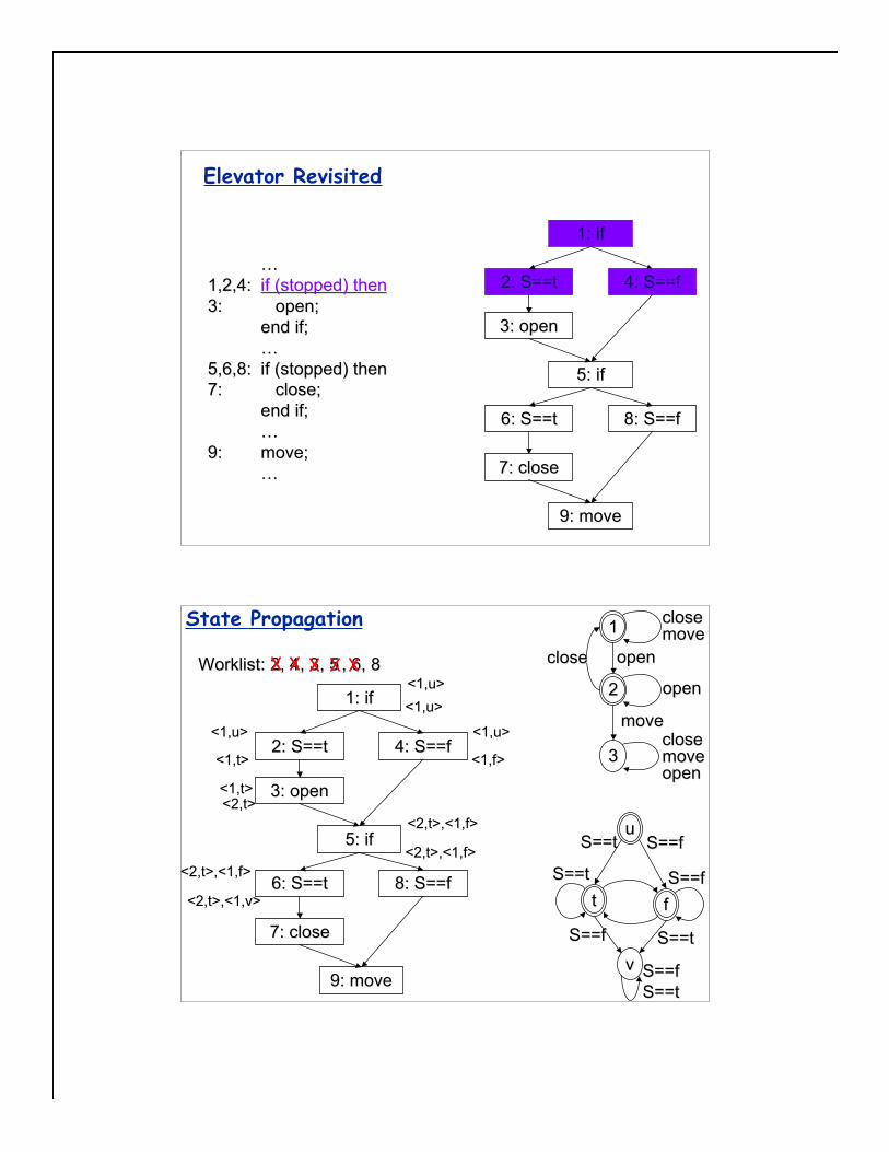
Elevator Revisited
1: if
2: S==t
5: if5: if
9: move9: move
4: S==f
3: open3: open
6: S==t6: S==t 8: S==f8: S==f
7: close7: close
……1,2,4:1,2,4: if (stopped) thenif (stopped) then3:3: open;open;
end if;end if;……
5,6,8:5,6,8: if (stopped) thenif (stopped) then7:7: close;close;
end if;end if;……
9:9: move;move;……
, 6, 8, 6, 8, 5, 5, 3, 3
State Propagation
2: S==t2: S==t
1: if1: if
5: if5: if
9: move9: move
4: S==f4: S==f
3: open3: open
6: S==t6: S==t 8: S==f8: S==f
7: close7: close
11
22
33
closeclose openopen
movemovecloseclosemovemoveopenopen
openopen
closeclosemovemove
tt
vv
S==tS==t
ff
uuS==fS==f
S==fS==f S==tS==t
S==tS==t S==fS==f
S==fS==fS==tS==t
<2,t>,<1,v><2,t>,<1,v>
WorklistWorklist: 2, 4: 2, 4
<1,u><1,u>
<1,t><1,t>
<2,t><2,t>
<1,f><1,f>
<2,t>,<1,f><2,t>,<1,f>
<1,u><1,u>
<1,u><1,u> <1,u><1,u>
<1,t><1,t>
<2,t>,<1,f><2,t>,<1,f>
<2,t>,<1,f><2,t>,<1,f>
1: if
5: if
, 6, 8, 6, 8, 5, 5, 3, 3
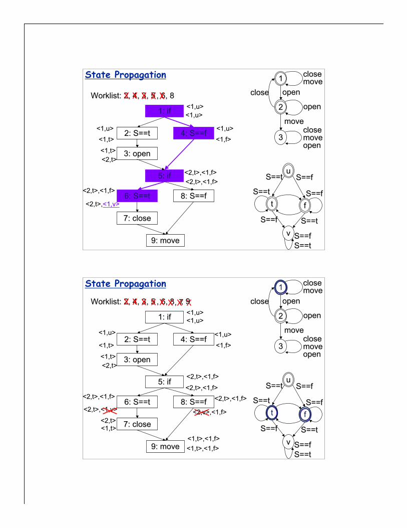
State Propagation
2: S==t2: S==t
9: move9: move
4: S==f
3: open3: open
6: S==t 8: S==f8: S==f
7: close7: close
<2,t>,<2,t>,<1,v><1,v>
WorklistWorklist: 2, 4: 2, 4
<1,u><1,u>
<1,t><1,t>
<2,t><2,t>
<1,f><1,f>
<2,t>,<1,f><2,t>,<1,f>
11
22
33
closeclose openopen
movemovecloseclosemovemoveopenopen
openopen
closeclosemovemove
tt
vv
S==tS==t
ff
uuS==fS==f
S==fS==f S==tS==t
S==tS==t S==fS==f
S==fS==fS==tS==t
<1,u><1,u>
<1,u><1,u><1,u><1,u>
<1,t><1,t>
<2,t>,<1,f><2,t>,<1,f>
<2,t>,<1,f><2,t>,<1,f>
State Propagation 1
22
33
closeclose openopen
movemovecloseclosemovemoveopenopen
openopen
closeclosemovemove
t
vv
S==tS==t
f
uuS==fS==f
S==fS==f S==tS==t
S==tS==t S==fS==f
S==fS==fS==tS==t
1: if1: if
5: if5: if
, 6, 8, 6, 8, 5, 5, 3, 3
2: S==t2: S==t
9: move9: move
4: S==f4: S==f
3: open3: open
6: S==t6: S==t 8: S==f8: S==f
7: close7: close
<2,t>,<1,v><2,t>,<1,v>
WorklistWorklist: 2, 4: 2, 4
<1,u><1,u>
<1,t><1,t>
<2,t><2,t>
<1,f><1,f>
<2,t>,<1,f><2,t>,<1,f>
, 7, 7<1,u><1,u>
<1,u><1,u><1,u><1,u>
<1,t><1,t>
<2,t>,<1,f><2,t>,<1,f>
<2,t>,<1,f><2,t>,<1,f> <2,t>,<1,f><2,t>,<1,f>
<1,t><1,t>
<2,v>,<1,f><2,v>,<1,f>
<1,t>,<1,f><1,t>,<1,f>
<2,t><2,t>
<1,t>,<1,f><1,t>,<1,f>
, 9, 9
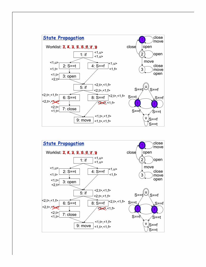
State Propagation 1
22
33
closeclose openopen
movemovecloseclosemovemoveopenopen
openopen
closeclosemovemove
t
vv
S==tS==t
f
uuS==fS==f
S==fS==f S==tS==t
S==tS==t S==fS==f
S==fS==fS==tS==t
1: if1: if
5: if5: if
, 6, 8, 6, 8, 5, 5, 3, 3
2: S==t2: S==t
9: move9: move
4: S==f4: S==f
3: open3: open
6: S==t6: S==t 8: S==f8: S==f
7: close7: close
<2,t>,<1,v><2,t>,<1,v>
WorklistWorklist: 2, 4: 2, 4
<1,u><1,u>
<1,t><1,t>
<2,t><2,t>
<1,f><1,f>
<2,t>,<1,f><2,t>,<1,f>
, 7, 9, 7, 9<1,u><1,u>
<1,u><1,u><1,u><1,u>
<1,t><1,t>
<2,t>,<1,f><2,t>,<1,f>
<2,t>,<1,f><2,t>,<1,f> <2,t>,<1,f><2,t>,<1,f>
<1,t><1,t>
<2,v>,<1,f><2,v>,<1,f>
<1,t>,<1,f><1,t>,<1,f>
<2,t><2,t>
<1,t>,<1,f><1,t>,<1,f>
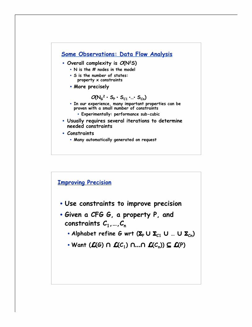
Some Observations: Data Flow Analysis• Overall complexity is O(N2S)
• N is the # nodes in the model• S is the number of states:
property x constraints• More precisely
O(NG2 ⋅ SP ⋅ SC1 ⋅…⋅ SCn)
• In our experience, many important properties can beproven with a small number of constraints• Experimentally: performance sub-cubic
• Usually requires several iterations to determineneeded constraints
• Constraints• Many automatically generated on request
Improving Precision
• Use constraints to improve precision• Given a CFG G, a property P, andconstraints C1,…,Cn
• Alphabet refine G wrt (ΣP ∪ ΣC1 ∪ … ∪ ΣCn)
• Want (L(G) ∩ L(C1) ∩…∩ L(Cn)) ⊆ L(P)
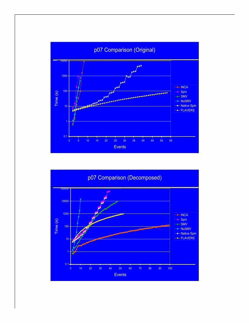
p07 Comparison (Original)
0.1
1
10
100
1000
10000
0 5 10 15 20 25 30 35 40 45 50 55
Events
Tim
e (
s)
INCA
Spin
SMV
NuSMV
Native Spin
FLAVERS
p07 Comparison (Decomposed)
0.1
1
10
100
1000
10000
100000
0 10 20 30 40 50 60 70 80 90 100
Events
Tim
e (
s)
INCA
Spin
SMV
NuSMV
Native Spin
FLAVERS
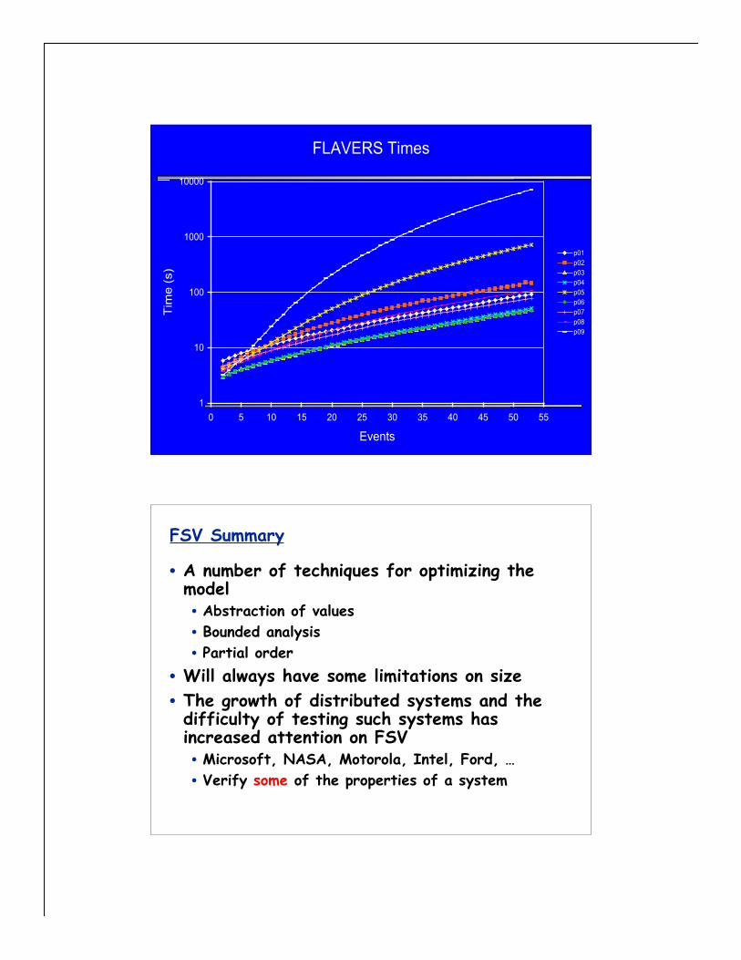
FLAVERS Times
1
10
100
1000
10000
0 5 10 15 20 25 30 35 40 45 50 55
Events
Tim
e (
s)
p01
p02
p03
p04
p05
p06
p07
p08
p09
FSV Summary
• A number of techniques for optimizing themodel• Abstraction of values• Bounded analysis• Partial order
• Will always have some limitations on size• The growth of distributed systems and thedifficulty of testing such systems hasincreased attention on FSV• Microsoft, NASA, Motorola, Intel, Ford, …• Verify some of the properties of a system