Finite Volume Methods (1D-2D)aleon3/courses/Transient_flows/Lectures...Finite Volume Methods (1D-2D) Adapted from Notes on “Transient Flows” by Arturo Leon and Shallow-Water equations

Finite Volume Methods(1D-2D)

Adapted from Notes on “Transient Flows” by Arturo Leon and Shallow-Water equations by Andrew Sleigh

Arturo Leon, Oregon State University (Fall 2013)

11/26/20131 © Arturo S. Leon, OSU

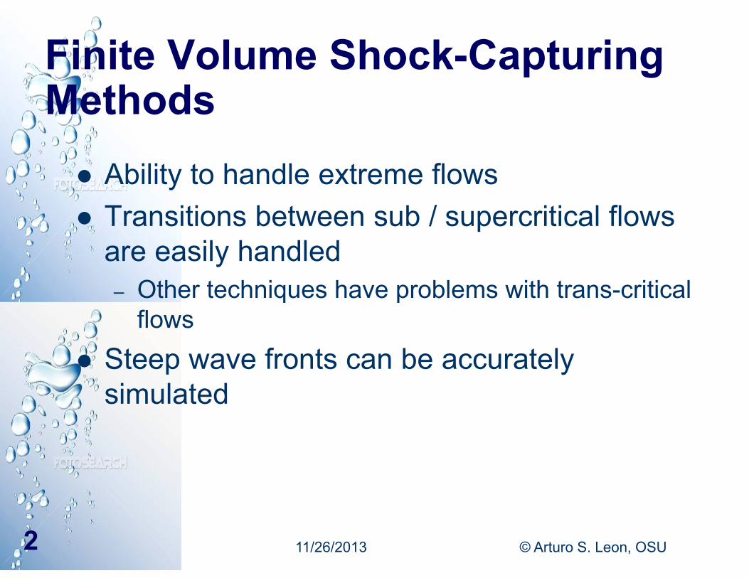
Ability to handle extreme flows Transitions between sub / supercritical flows

are easily handled– Other techniques have problems with trans-critical

flows Steep wave fronts can be accurately

simulated

11/26/2013 © Arturo S. Leon, OSU2

Finite Volume Shock-Capturing Methods

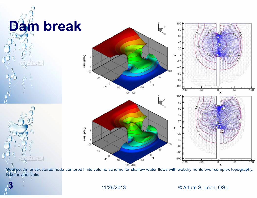
Dam break


Source: An unstructured node-centered finite volume scheme for shallow water flows with wet/dry fronts over complex topography, Nikolos and Delis

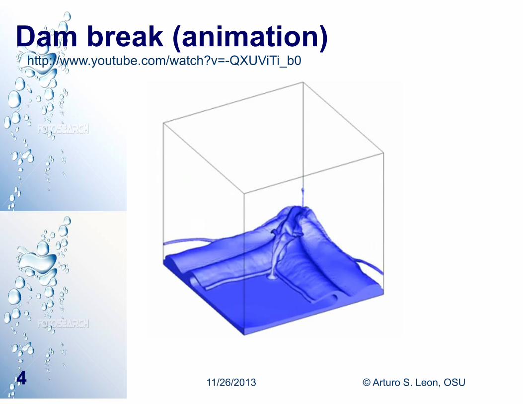
Dam break (animation)


http://www.youtube.com/watch?v=-QXUViTi_b0

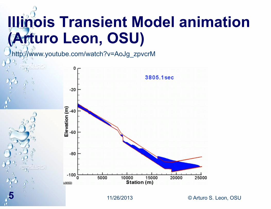
Illinois Transient Model animation (Arturo Leon, OSU)


http://www.youtube.com/watch?v=AoJg_zpvcrM

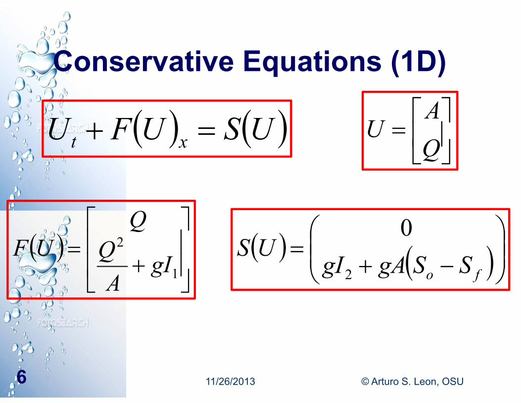
Conservative Equations (1D)

USUFU xt

QA

U

1

2

gIAQQ

UF

fo SSgAgI

US2

0


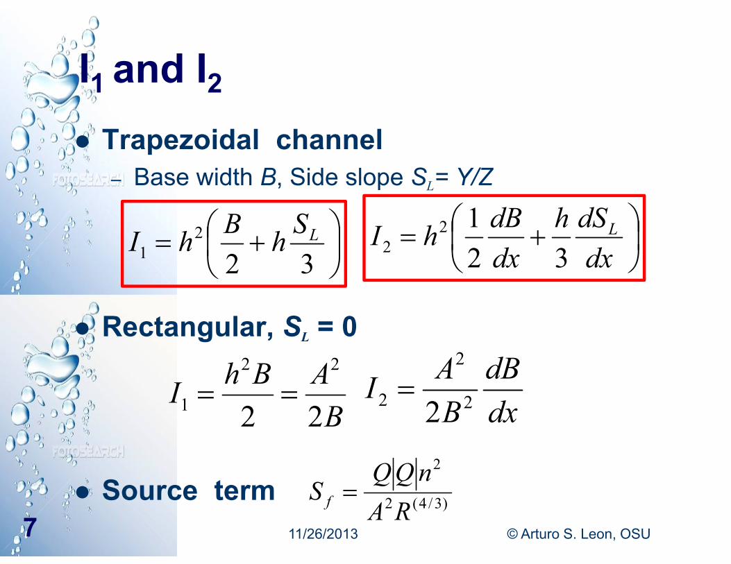
I1 and I2 Trapezoidal channel

– Base width B, Side slope SL= Y/Z

Rectangular, SL = 0

Source term

322

1LShBhI

dxdSh

dxdBhI L

3212

2

BABhI22

22

1 dxdB

BAI 2

2

2 2

)3/4(2

2

RAnQQ

S f 11/26/2013 © Arturo S. Leon, OSU7

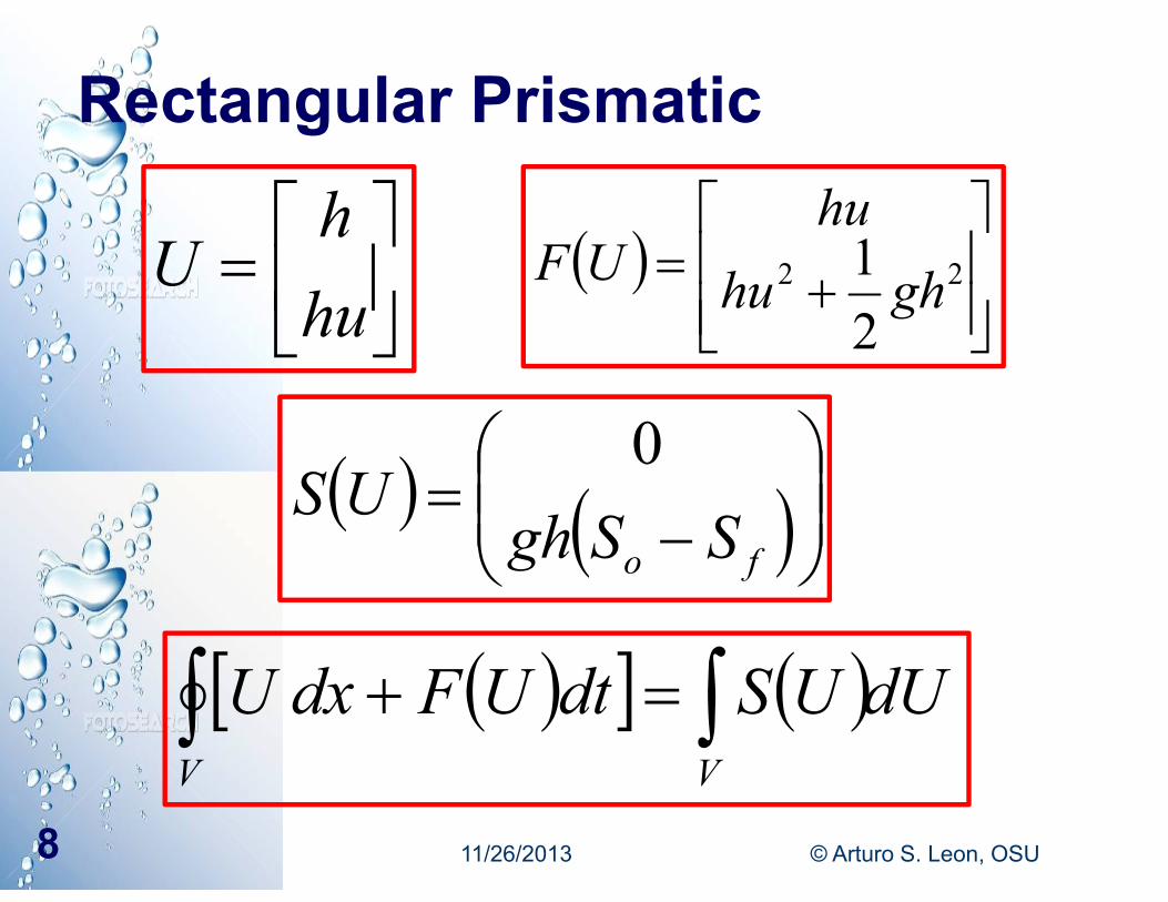
Rectangular Prismatic

huh

U

22

21 ghhuhu

UF

fo SSgh

US0

dUUSdtUFdxUVV


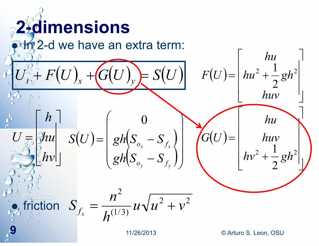
2-dimensions In 2-d we have an extra term:

friction

USUGUFU yxt

hvhuh

U

huv

ghhuhu

UF 22

21

22

21 ghhv

huvhu

UG

yy

xx

fo

fo

SSghSSghUS

0

22)3/1(

2

vuuhnS

xf


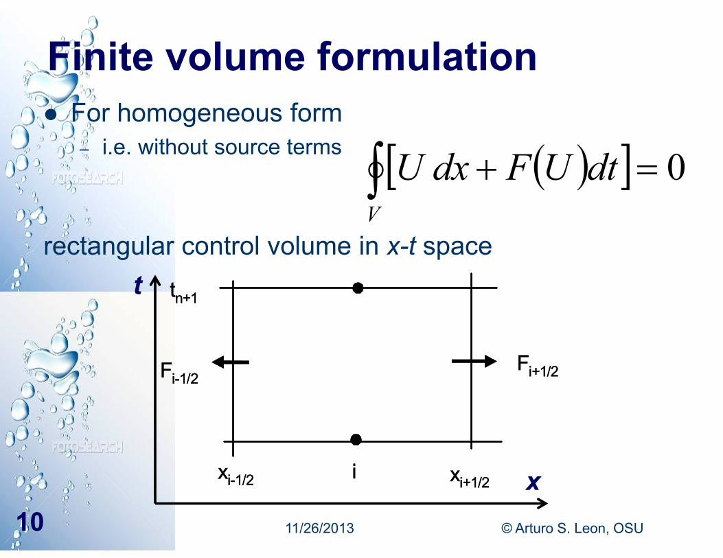
Finite volume formulation For homogeneous form

– i.e. without source terms

rectangular control volume in x-t space

0V

dtUFdxU


xi-1/2 xi+1/2

tn+1

i

Fi-1/2Fi+1/2

xi-1/2 xi+1/2

tn+1

i

Fi-1/2Fi+1/2

t

x

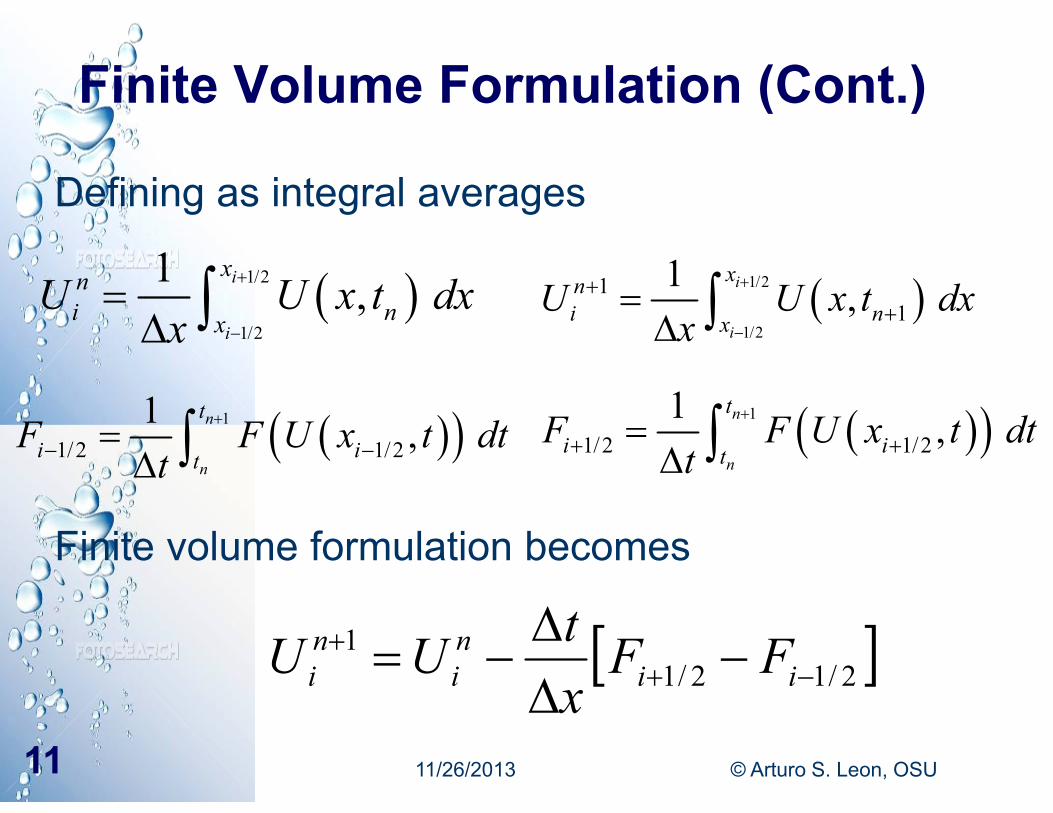
Finite Volume Formulation (Cont.)

Defining as integral averages

Finite volume formulation becomes

1/2

1/2

1 ,i

i

xni nx

U U x t dxx

1/2

1/2

11

1 ,i

i

xni nx

U U x t dxx

1

1/2 1/21 ,n

n

t

i itF F U x t dt

t

1

1/2 1/21 ,n

n

t

i itF F U x t dt

t

2/12/11

iini

ni FF

xtUU


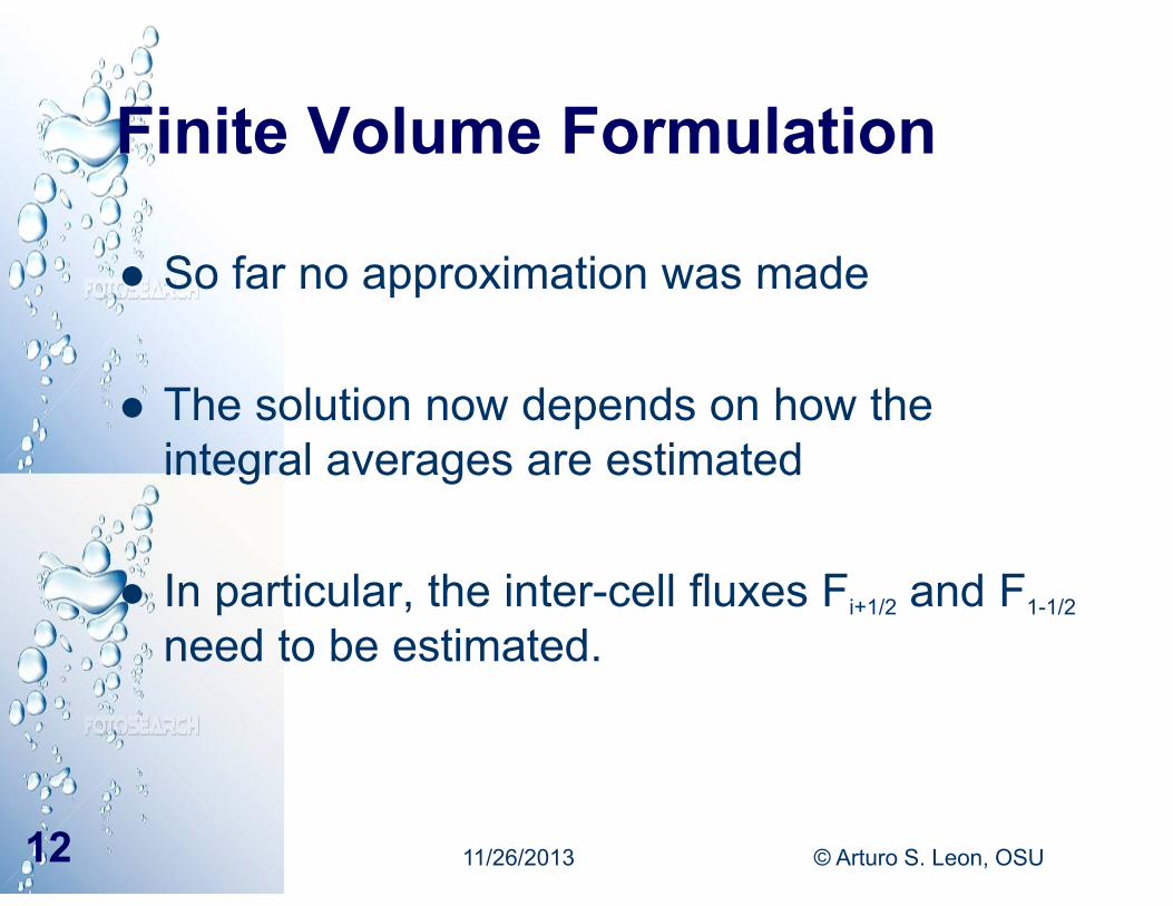
Finite Volume Formulation

So far no approximation was made

The solution now depends on how the integral averages are estimated

In particular, the inter-cell fluxes Fi+1/2 and F1-1/2

need to be estimated.


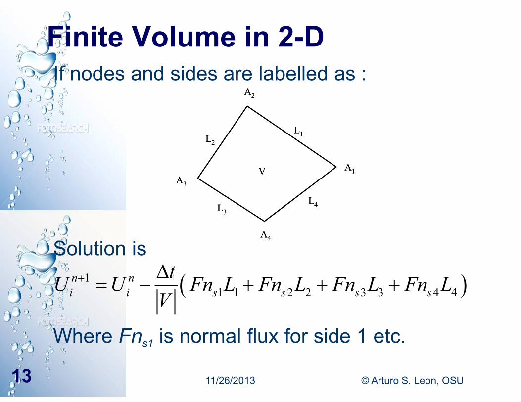
Finite Volume in 2-DIf nodes and sides are labelled as :

Solution is

Where Fns1 is normal flux for side 1 etc.

A1A3

A2

A4

V

L4L3

L2

L1

A1A3

A2

A4

V

L4L3

L2

L1

11 1 2 2 3 3 4 4

n ni i s s s s

tU U Fn L Fn L Fn L Fn LV


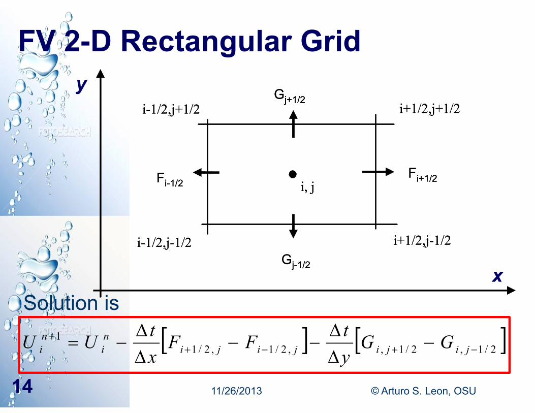
FV 2-D Rectangular Grid

Solution is

Fi-1/2Fi+1/2

Gj-1/2

Gj+1/2

i+1/2,j-1/2

i-1/2,j+1/2

i-1/2,j-1/2

i+1/2,j+1/2

i, jFi-1/2Fi+1/2

Gj-1/2

Gj+1/2

i+1/2,j-1/2

i-1/2,j+1/2

i-1/2,j-1/2

i+1/2,j+1/2

i, j

2/1,2/1,,2/1,2/11

jijijijini

ni GG

ytFF

xtUU


y

x

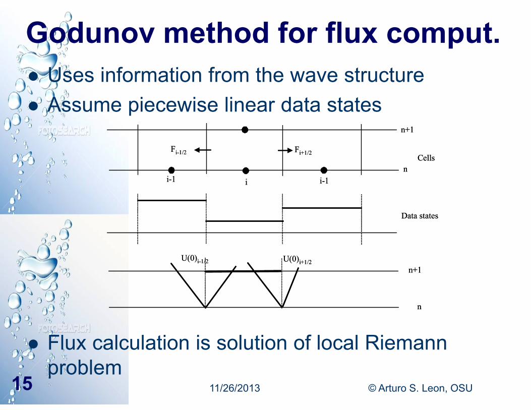
Godunov method for flux comput. Uses information from the wave structure Assume piecewise linear data states

Flux calculation is solution of local Riemann problem

n

n+1

i-1 i i-1

Fi+1/2Fi-1/2Cells

Data states

n+1

n

U(0)i+1/2U(0)i-1/2

n

n+1

i-1 i i-1

Fi+1/2Fi-1/2Cells

Data states

n+1

n

U(0)i+1/2U(0)i-1/2


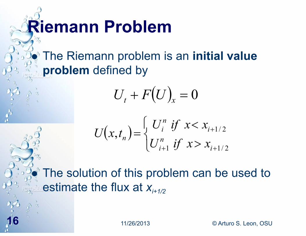
Riemann Problem The Riemann problem is an initial value

problem defined by

The solution of this problem can be used to estimate the flux at xi+1/2

0 xt UFU

2/11

2/1,i

ni

ini

n xxifUxxifU

txU


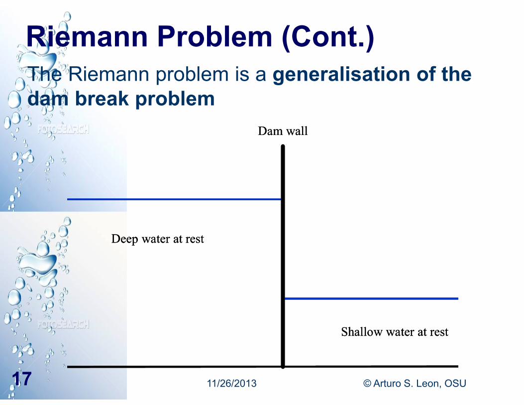
Riemann Problem (Cont.)The Riemann problem is a generalisation of the dam break problem

Dam wall

Deep water at rest

Shallow water at rest

Dam wall

Deep water at rest

Shallow water at rest


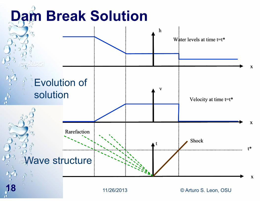
Dam Break Solution

Evolution of solution

x

x

x

Water levels at time t=t*

t*t

Velocity at time t=t*

v

h

Shock

Rarefaction

xx

xx

xx

Water levels at time t=t*

t*t

Velocity at time t=t*

v

h

Shock

Rarefaction

Wave structure


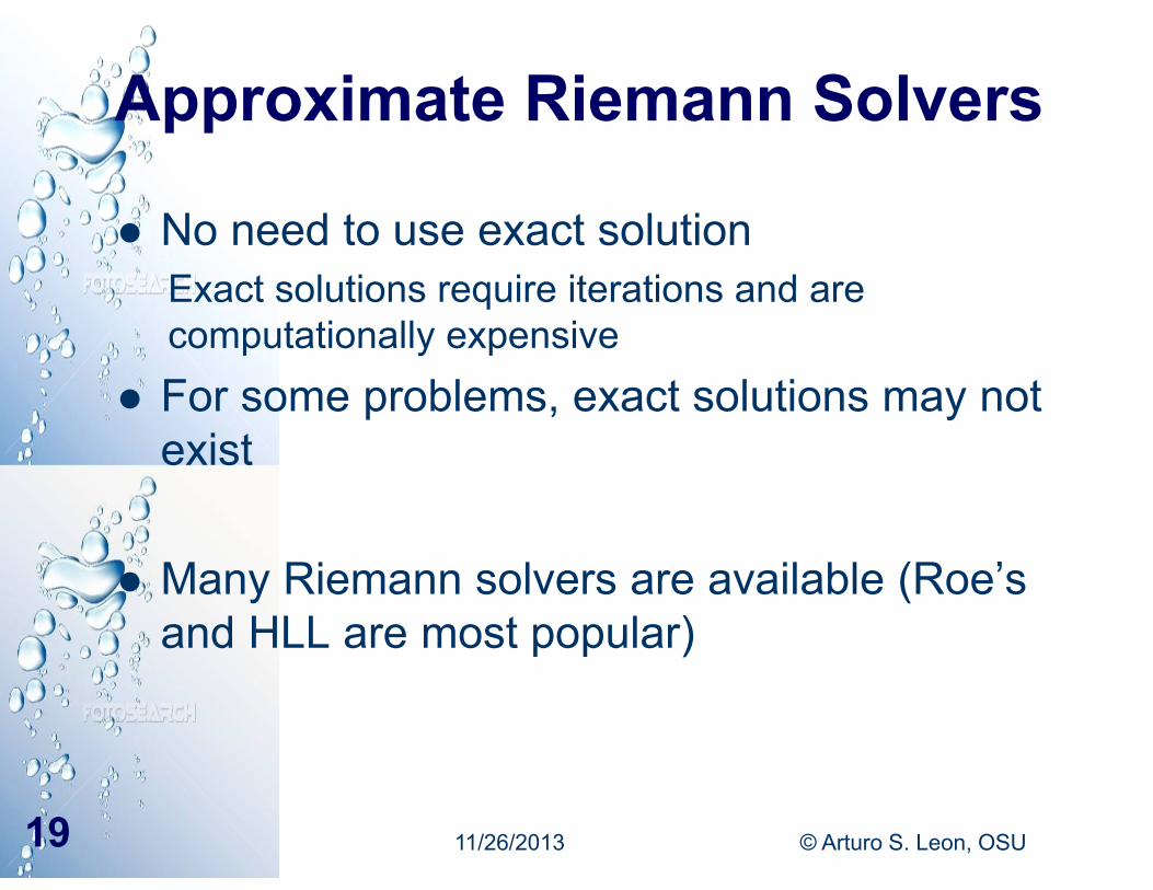
Approximate Riemann Solvers

No need to use exact solutionExact solutions require iterations and are computationally expensive

For some problems, exact solutions may not exist

Many Riemann solvers are available (Roe’s and HLL are most popular)


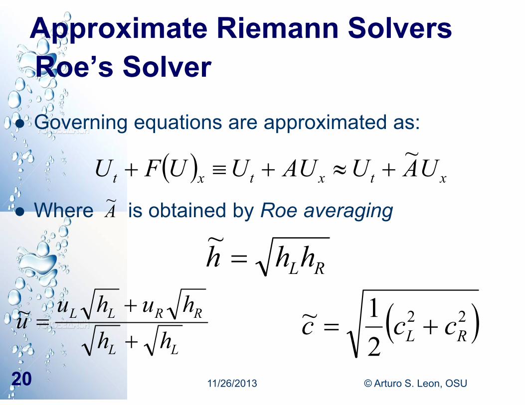
Roe’s Solver

Governing equations are approximated as:

Where is obtained by Roe averaging

xtxtxt UAUAUUUFU ~

A~

LL

RRLL

hhhuhu

u

~

RLhhh ~

22

21~

RL ccc


Approximate Riemann Solvers

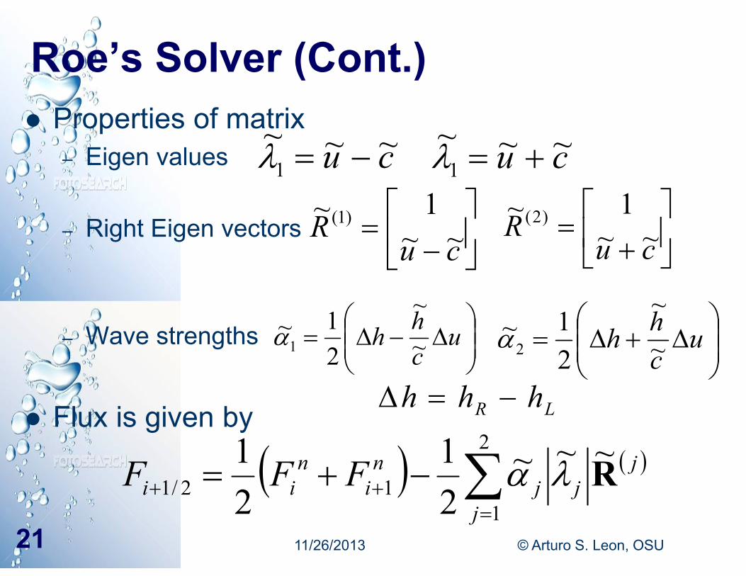
Roe’s Solver (Cont.) Properties of matrix

– Eigen values

– Right Eigen vectors

– Wave strengths

Flux is given by

cu ~~~1 cu ~~~

1

cu

R ~~1~ )1(

cu

R ~~1~ )2(

u

chh ~

~

21~

1

u

chh ~

~

21~

2

LR hhh

2

112/1

~~~21

21

j

jjj

ni

nii FFF R


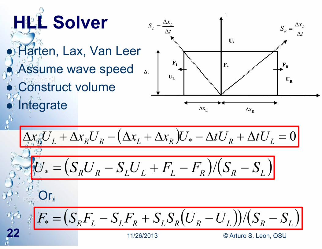
HLL Solver Harten, Lax, Van Leer Assume wave speed Construct volume Integrate

Or,

t

URUL

U*

FRFL F*

t

xL xR

t

URUL

U*

FRFL F*

t

xL xR

0* LRRLRRLL tUtUUxxUxUx

txS L

L

txS R

R

LRRLLLRR SSFFUSUSU /*

LRLRRLRLLR SSUUSSFSFSF /*11/26/2013 © Arturo S. Leon, OSU22

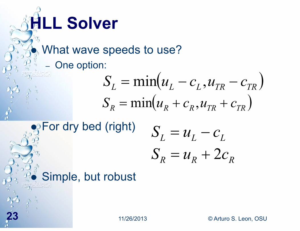
HLL Solver What wave speeds to use?

– One option:

For dry bed (right)

Simple, but robust

TRTRLLL cucuS ,min TRTRRRR cucuS ,min

LLL cuS

RRR cuS 2


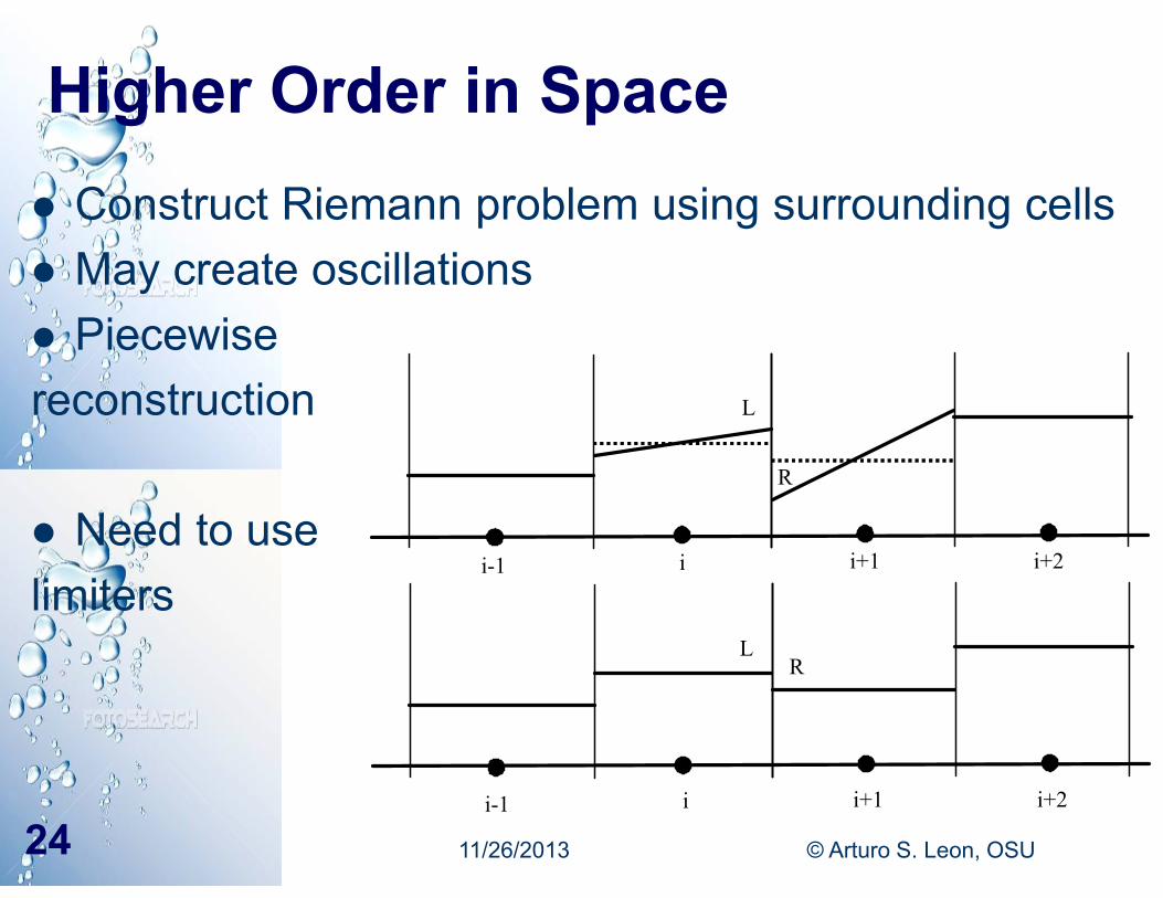
Higher Order in Space Construct Riemann problem using surrounding cells May create oscillations Piecewise reconstruction

Need to use limiters

i-1 i i+1 i+2

i-1 i i+1 i+2

L

R

LR


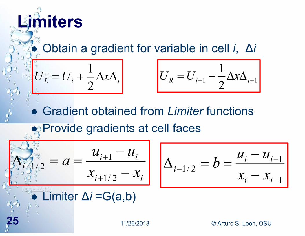
Limiters Obtain a gradient for variable in cell i, ∆i

Gradient obtained from Limiter functions Provide gradients at cell faces

Limiter ∆i =G(a,b)

iiL xUU 21

11 21

iiR xUU

ii

iii xx

uua

2/1

12/1

1

12/1

ii

iii xx

uub


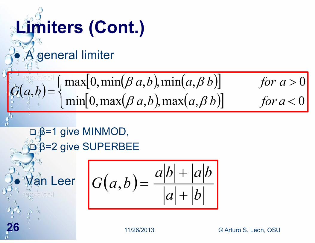
Limiters (Cont.) A general limiter

β=1 give MINMOD, β=2 give SUPERBEE

Van Leer

0,max,,max,0min0,min,,min,0max

,aforbabaaforbaba

baG

bababa

baG

,


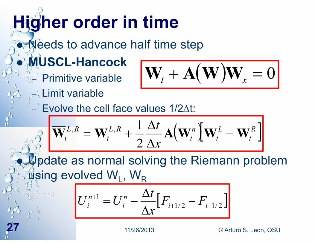
Higher order in time Needs to advance half time step MUSCL-Hancock

– Primitive variable– Limit variable– Evolve the cell face values 1/2t:

Update as normal solving the Riemann problem using evolved WL, WR

0 xt WWAW

RiLi

ni

RLi

RLi x

t WWWAWW

21,,

2/12/11

iini

ni FF

xtUU


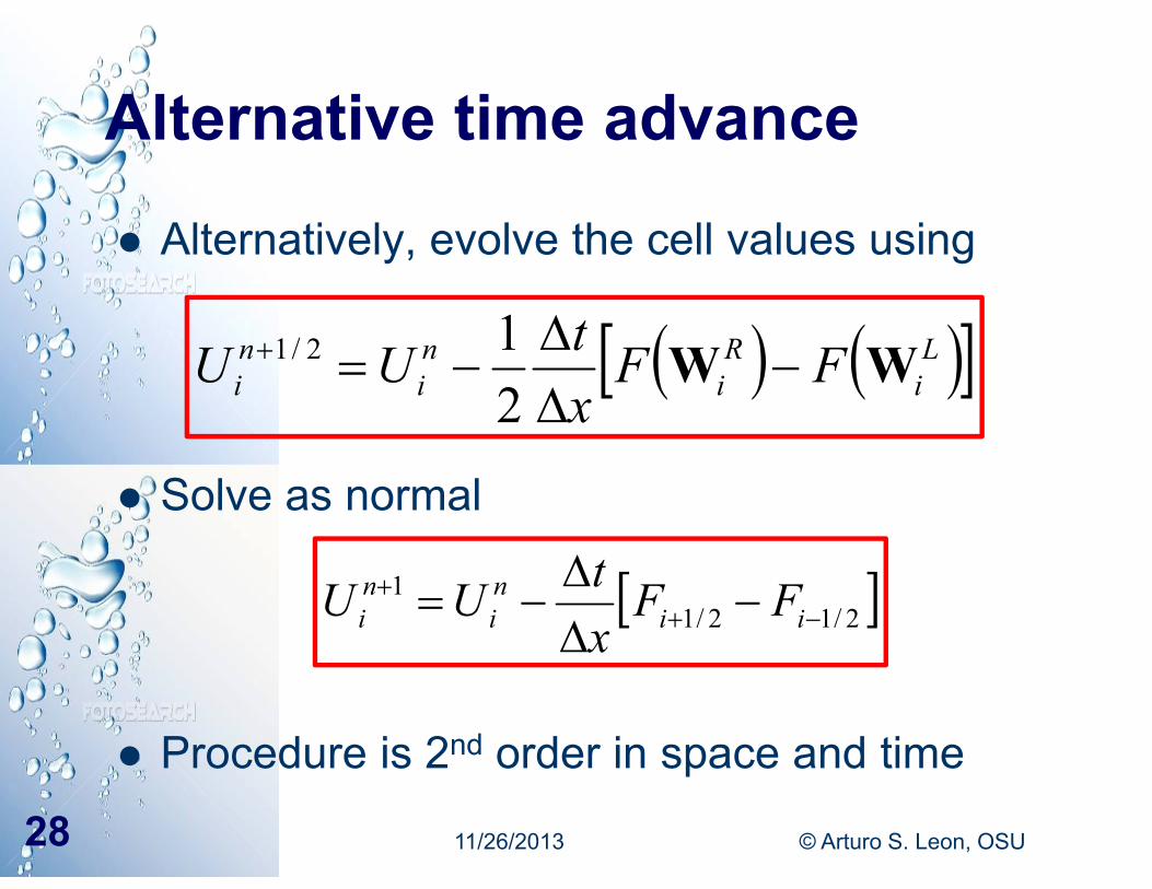
Alternative time advance

Alternatively, evolve the cell values using

Solve as normal

Procedure is 2nd order in space and time

Li

Ri

ni

ni FF

xtUU WW

212/1

2/12/11

iini

ni FF

xtUU


Wet / Dry Fonts

Wet / Dry fronts are difficult– Source of error– Source of instability

Found in: Filling of storm-water and combined sewer

systems Flooding - inundation


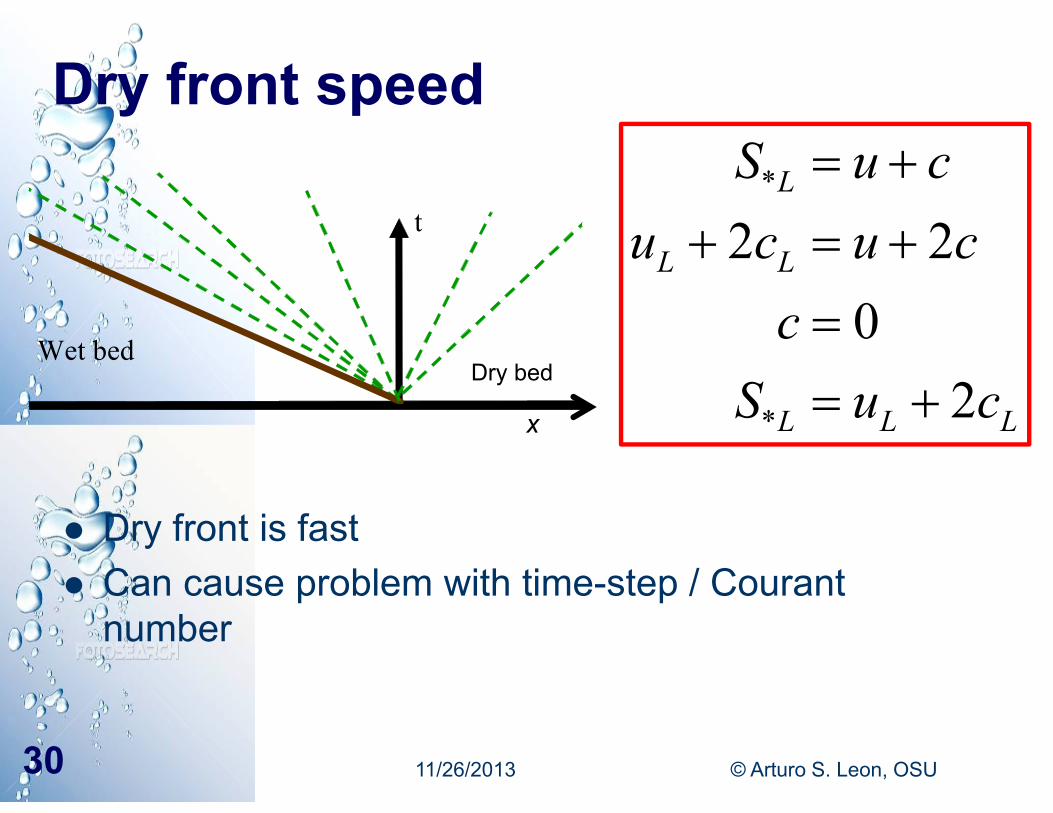
Dry front speed

Dry front is fast Can cause problem with time-step / Courant

number

*

*

2 20

2

L

L L

L L L

S u cu c u c

cS u c


t

Wet bed

x

Dry bed

Solutions for wet/dry fronts

Most popular way is to artificially wet bed Provide a small water depth with zero

velocity Can drastically affect front speed Need to be very careful about dividing by

zero


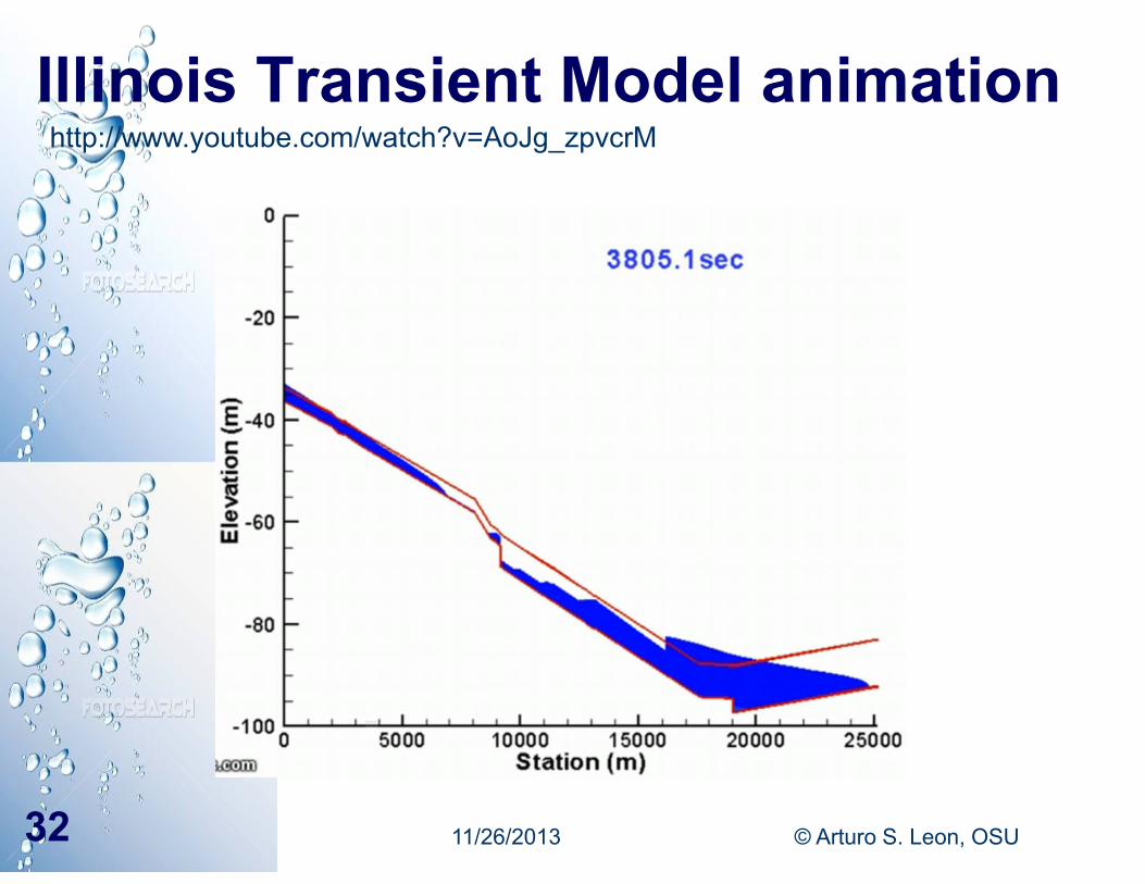
Illinois Transient Model animation


http://www.youtube.com/watch?v=AoJg_zpvcrM

Documents

Finite Volume Methods (1D-2D)aleon3/courses/Transient_flows/Lectures...Finite Volume Methods (1D-2D) Adapted from Notes on “Transient Flows” by Arturo Leon and Shallow-Water equations