Finite Volume Methods and Adaptive Refinementfor Tsunami Propagation and Inundation

David L. George

A dissertation submitted in partial fulfillmentof the requirements for the degree of

Doctor of Philosophy

University of Washington

2006

Program Authorized to Offer Degree: Applied Mathematics

University of WashingtonGraduate School

This is to certify that I have examined this copy of a doctoral dissertation by

David L. George

and have found that it is complete and satisfactory in all respects,and that any and all revisions required by the final

examining committee have been made.

Chair of the Supervisory Committee:

Randall J. LeVeque

Reading Committee:

Randall J. LeVeque

Christopher S. Bretherton

Vasilli V. Titov

Date:

In presenting this dissertation in partial fulfillment of the requirements for the doctoraldegree at the University of Washington, I agree that the Library shall make its copiesfreely available for inspection. I further agree that extensive copying of this dissertation isallowable only for scholarly purposes, consistent with “fair use” as prescribed in the U.S.Copyright Law. Requests for copying or reproduction of this dissertation may be referredto Proquest Information and Learning, 300 North Zeeb Road, Ann Arbor, MI 48106-1346,1-800-521-0600, to whom the author has granted “the right to reproduce and sell (a) copiesof the manuscript in microform and/or (b) printed copies of the manuscript made frommicroform.”

Signature

Date

University of Washington

Abstract

Finite Volume Methods and Adaptive Refinementfor Tsunami Propagation and Inundation

David L. George

Chair of the Supervisory Committee:Professor Randall J. LeVeque

Department of Applied Mathematics

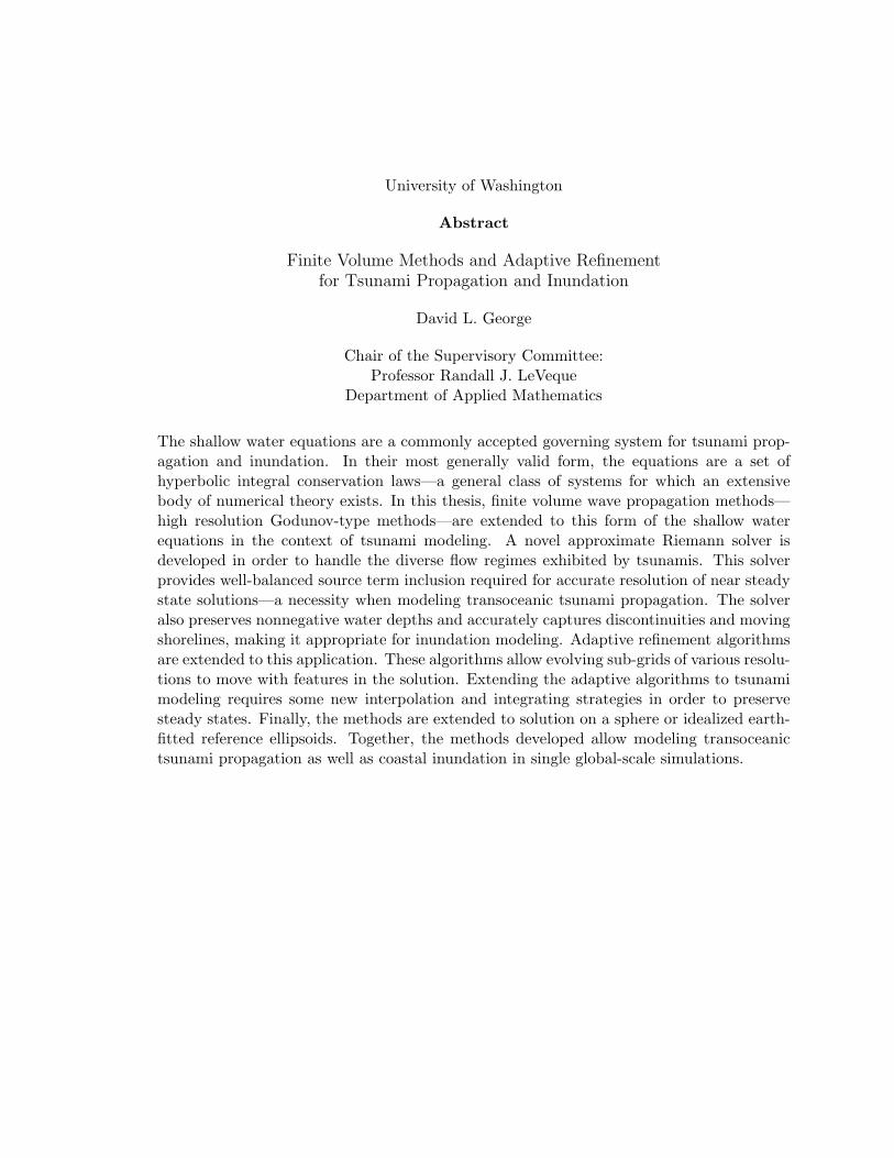
The shallow water equations are a commonly accepted governing system for tsunami prop-agation and inundation. In their most generally valid form, the equations are a set ofhyperbolic integral conservation laws—a general class of systems for which an extensivebody of numerical theory exists. In this thesis, finite volume wave propagation methods—high resolution Godunov-type methods—are extended to this form of the shallow waterequations in the context of tsunami modeling. A novel approximate Riemann solver isdeveloped in order to handle the diverse flow regimes exhibited by tsunamis. This solverprovides well-balanced source term inclusion required for accurate resolution of near steadystate solutions—a necessity when modeling transoceanic tsunami propagation. The solveralso preserves nonnegative water depths and accurately captures discontinuities and movingshorelines, making it appropriate for inundation modeling. Adaptive refinement algorithmsare extended to this application. These algorithms allow evolving sub-grids of various resolu-tions to move with features in the solution. Extending the adaptive algorithms to tsunamimodeling requires some new interpolation and integrating strategies in order to preservesteady states. Finally, the methods are extended to solution on a sphere or idealized earth-fitted reference ellipsoids. Together, the methods developed allow modeling transoceanictsunami propagation as well as coastal inundation in single global-scale simulations.

TABLE OF CONTENTS

Page

List of Figures . . . . . . . . . . . . . . . . . . . . . . . . . . . . . . . . . . . . . . . . iv

Chapter 1: Introduction . . . . . . . . . . . . . . . . . . . . . . . . . . . . . . . . . 11.1 Statement of Purpose . . . . . . . . . . . . . . . . . . . . . . . . . . . . . . . 11.2 Tsunami Modeling with the Shallow Water Equations . . . . . . . . . . . . . 11.3 Numerical Challenges . . . . . . . . . . . . . . . . . . . . . . . . . . . . . . . 31.4 Thesis Overview . . . . . . . . . . . . . . . . . . . . . . . . . . . . . . . . . . 4

Chapter 2: Hyperbolic Conservation Laws and Related Systems . . . . . . . . . . 62.1 The Shallow Water Equations . . . . . . . . . . . . . . . . . . . . . . . . . . . 62.2 Hyperbolic Conservation Laws . . . . . . . . . . . . . . . . . . . . . . . . . . 72.3 Discontinuities and Weak Solutions . . . . . . . . . . . . . . . . . . . . . . . . 82.4 Linear and Quasilinear Hyperbolic Systems . . . . . . . . . . . . . . . . . . . 102.5 Riemann Problems . . . . . . . . . . . . . . . . . . . . . . . . . . . . . . . . . 112.6 Balance Laws and Source Terms . . . . . . . . . . . . . . . . . . . . . . . . . 17

Chapter 3: Finite Volume Methods and Wave Propagation Algorithms . . . . . . 193.1 Finite Volume Methods for Conservation Laws . . . . . . . . . . . . . . . . . 193.2 Godunov-Type Methods . . . . . . . . . . . . . . . . . . . . . . . . . . . . . . 203.3 Approximate Riemann Solvers . . . . . . . . . . . . . . . . . . . . . . . . . . 213.4 Wave Propagation Algorithms . . . . . . . . . . . . . . . . . . . . . . . . . . . 243.5 Depth Positivity and Vacuum States . . . . . . . . . . . . . . . . . . . . . . . 263.6 Numerical Treatment of Source Terms . . . . . . . . . . . . . . . . . . . . . . 293.7 High Resolution Methods . . . . . . . . . . . . . . . . . . . . . . . . . . . . . 313.8 Extension to Multiple Dimensions . . . . . . . . . . . . . . . . . . . . . . . . 333.9 Preserving Positivity by Limiting . . . . . . . . . . . . . . . . . . . . . . . . . 34

Chapter 4: The Shallow Water Equations . . . . . . . . . . . . . . . . . . . . . . . 364.1 The Shallow Water Approximation and Derivation . . . . . . . . . . . . . . . 364.2 The Riemann Problem . . . . . . . . . . . . . . . . . . . . . . . . . . . . . . . 39

i

4.3 Dry State Riemann Problems . . . . . . . . . . . . . . . . . . . . . . . . . . . 444.4 Steady States and Source Terms . . . . . . . . . . . . . . . . . . . . . . . . . 47

Chapter 5: Numerical Tsunami Modeling . . . . . . . . . . . . . . . . . . . . . . . 585.1 Tsunami Generation and Governing Assumptions . . . . . . . . . . . . . . . . 585.2 The Diverse Regimes of Tsunami Flow . . . . . . . . . . . . . . . . . . . . . . 605.3 Deep Ocean Propagation . . . . . . . . . . . . . . . . . . . . . . . . . . . . . . 605.4 Shoaling: Bores and Discontinuities . . . . . . . . . . . . . . . . . . . . . . . . 635.5 Shorelines and Inundation . . . . . . . . . . . . . . . . . . . . . . . . . . . . . 64

Chapter 6: Approximate Augmented Riemann Solvers for the Shallow Water Equa-tions and Tsunami Modeling . . . . . . . . . . . . . . . . . . . . . . . 66

6.1 Augmented Systems . . . . . . . . . . . . . . . . . . . . . . . . . . . . . . . . 666.2 An Approximate Riemann Solver Based on an Augmented System . . . . . . 696.3 Shock Preservation and Relation to the Roe Solver . . . . . . . . . . . . . . . 716.4 Source Terms and Well-Balancing . . . . . . . . . . . . . . . . . . . . . . . . . 726.5 Preserving Positivity and Relation to the HLLE Solver . . . . . . . . . . . . . 756.6 The Resonant Problem and Near-Sonic Problems . . . . . . . . . . . . . . . . 806.7 Rarefactions and Entropy Fixes . . . . . . . . . . . . . . . . . . . . . . . . . . 816.8 Inundation . . . . . . . . . . . . . . . . . . . . . . . . . . . . . . . . . . . . . 876.9 Extension to the Two-Dimensional Problem . . . . . . . . . . . . . . . . . . . 93

Chapter 7: Adaptive Mesh Refinement for Tsunami Modeling . . . . . . . . . . . 947.1 Adaptive Mesh Refinement for Hyperbolic Systems . . . . . . . . . . . . . . . 957.2 Maintaining Conservation and Steady States for Tsunami Modeling . . . . . 967.3 Shorelines and Shallow Regions . . . . . . . . . . . . . . . . . . . . . . . . . . 1027.4 Time Refinement . . . . . . . . . . . . . . . . . . . . . . . . . . . . . . . . . . 108

Chapter 8: Modeling Tsunamis on the Earth . . . . . . . . . . . . . . . . . . . . . 1098.1 General Quadrilateral Grids on a Flat Surface . . . . . . . . . . . . . . . . . . 1098.2 The Shallow Water Equations on Latitude-Longitude Grids . . . . . . . . . . 1138.3 Coriolis Forces . . . . . . . . . . . . . . . . . . . . . . . . . . . . . . . . . . . 1188.4 Frictional Forces . . . . . . . . . . . . . . . . . . . . . . . . . . . . . . . . . . 119

Chapter 9: Miscellaneous Numerical Results . . . . . . . . . . . . . . . . . . . . . 1209.1 Some One-Dimensional Test Problems . . . . . . . . . . . . . . . . . . . . . . 1209.2 Benchmark Problems from the 3rd International Longwave Workshop . . . . 125

ii

9.3 Adaptive Mesh Refinement for the Conical Island Test Problem . . . . . . . . 128

Chapter 10: Simulations of the 2004 Indian Ocean Tsunami . . . . . . . . . . . . . 13310.1 The 2004 Sumatra-Andaman Earthquake and Generation of the Tsunami . . 13310.2 A Three-Level Simulation For the Bay of Bengal . . . . . . . . . . . . . . . . 13810.3 A Fourth Level to Model Inundation at Madras, India . . . . . . . . . . . . . 140

Chapter 11: Conclusions and Future Directions . . . . . . . . . . . . . . . . . . . . 14411.1 Conclusions . . . . . . . . . . . . . . . . . . . . . . . . . . . . . . . . . . . . . 14411.2 Future Work . . . . . . . . . . . . . . . . . . . . . . . . . . . . . . . . . . . . 145

Bibliography . . . . . . . . . . . . . . . . . . . . . . . . . . . . . . . . . . . . . . . . . 146

Appendix A: TsunamiClaw User’s Guide . . . . . . . . . . . . . . . . . . . . . . . 154A.1 Introduction . . . . . . . . . . . . . . . . . . . . . . . . . . . . . . . . . . . . . 154A.2 General Features of TsunamiClaw . . . . . . . . . . . . . . . . . . . . . . . 154A.3 Running TsunamiClaw . . . . . . . . . . . . . . . . . . . . . . . . . . . . . . 155A.4 The TsunamiClaw library . . . . . . . . . . . . . . . . . . . . . . . . . . . . 155A.5 Application Directory . . . . . . . . . . . . . . . . . . . . . . . . . . . . . . . 156A.6 Data Input (setprob.data) . . . . . . . . . . . . . . . . . . . . . . . . . . . . 156A.7 Data Input (amr2ez.data) . . . . . . . . . . . . . . . . . . . . . . . . . . . . 159A.8 User Accessible Fortran Routines . . . . . . . . . . . . . . . . . . . . . . . . . 159A.9 The Computational Domain . . . . . . . . . . . . . . . . . . . . . . . . . . . . 160A.10 Bathymetry . . . . . . . . . . . . . . . . . . . . . . . . . . . . . . . . . . . . . 161A.11 Fault Models . . . . . . . . . . . . . . . . . . . . . . . . . . . . . . . . . . . . 162A.12 Time-Stepping and Anisotropic Refinement . . . . . . . . . . . . . . . . . . . 163A.13 Memory Allocation (bathcommon.i) . . . . . . . . . . . . . . . . . . . . . . . 164A.14 Data Output . . . . . . . . . . . . . . . . . . . . . . . . . . . . . . . . . . . . 164A.15 Matlab Graphics and Output Visualization . . . . . . . . . . . . . . . . . . . 165A.16 Acknowledgements . . . . . . . . . . . . . . . . . . . . . . . . . . . . . . . . . 166A.17 Usage Restrictions . . . . . . . . . . . . . . . . . . . . . . . . . . . . . . . . . 166

iii

LIST OF FIGURES

Figure Number Page

2.1 Cross section of a free surface flow governed by the shallow water equations. . 7

2.2 Characteristics of the three nonlinear wave-types in Riemann solutions areshown in the x–t plane. . . . . . . . . . . . . . . . . . . . . . . . . . . . . . . 13

2.3 Solutions to Riemann problems in the x–t plane. . . . . . . . . . . . . . . . . 14

2.4 Integral curves and Hugoniot loci of the shallow water equations. . . . . . . . 16

2.5 A solution to a one-dimensional normal Riemann problem of the two-dimensionalshallow water equations. . . . . . . . . . . . . . . . . . . . . . . . . . . . . . . 17

3.1 Comparison of the Roe and HLLE solvers for a Riemann problem with twostrong rarefactions. . . . . . . . . . . . . . . . . . . . . . . . . . . . . . . . . . 27

4.1 Deriving the shallow water equations from conservation principles. . . . . . . 38

4.2 Characterization of the Riemann problem for the shallow water equations byfunction evaluation. . . . . . . . . . . . . . . . . . . . . . . . . . . . . . . . . 43

4.3 An incipient cavitation Riemann problem. . . . . . . . . . . . . . . . . . . . . 44

4.4 Integral curves for the incipient cavitation problem. . . . . . . . . . . . . . . . 45

4.5 The incipient cavitation Riemann problem in the x-t plane. . . . . . . . . . . 46

4.6 An initial dry bed Riemann problem. . . . . . . . . . . . . . . . . . . . . . . . 47

4.7 The initial dry bed Riemann problems in the x-t plane. . . . . . . . . . . . . 48

4.8 A smoothed version of piecewise constant bathymetry. . . . . . . . . . . . . . 52

5.1 Tsunami scales: cross-section of the Bay of Bengal from a simulation of the2004 Sumatra-Andaman Tsunami. . . . . . . . . . . . . . . . . . . . . . . . . 61

5.2 Deviation from the physically common steady state. . . . . . . . . . . . . . . 62

5.3 Tsunami shoaling. . . . . . . . . . . . . . . . . . . . . . . . . . . . . . . . . . 63

6.1 Depths of steady state Riemann solution, for the motionless steady state andthe steady flow case with velocity. . . . . . . . . . . . . . . . . . . . . . . . . 74

6.2 Preserving the depth-positive-definite property of the augmented solver whenvariable bathymetry exists. . . . . . . . . . . . . . . . . . . . . . . . . . . . . 77

6.3 A common Riemann problem compared to one with a large rarefaction. . . . 82

6.4 A Riemann problem in the h-hu phase plane, showing the integral curve whenthere is a large rarefaction. . . . . . . . . . . . . . . . . . . . . . . . . . . . . 86

iv

6.5 Insufficient speed estimates for near-dry-state Riemann problems. . . . . . . . 88

6.6 A Riemann problem at the shoreline. . . . . . . . . . . . . . . . . . . . . . . . 90

6.7 The wall boundary condition Riemann problem as a test for the source term. 92

7.1 Adaptive mesh refinement with rectangular Cartesian grids . . . . . . . . . . 96

7.2 Interpolation and averaging between level l and (l + 1) grids. . . . . . . . . . 98

7.3 Interpolating the water depth from coarse grid cells to fine grid cells overnonlinear variable bathymetry. . . . . . . . . . . . . . . . . . . . . . . . . . . 101

7.4 Interpolation at the shoreline . . . . . . . . . . . . . . . . . . . . . . . . . . . 106

7.5 Adaptive mesh refinement around a shoreline. . . . . . . . . . . . . . . . . . . 107

8.1 Quadrilateral grids. . . . . . . . . . . . . . . . . . . . . . . . . . . . . . . . . . 112

8.2 Earth-fitted grids . . . . . . . . . . . . . . . . . . . . . . . . . . . . . . . . . . 114

8.3 Geographic latitude on an oblate ellipse . . . . . . . . . . . . . . . . . . . . . 116

9.1 Transcritical flow with a shock . . . . . . . . . . . . . . . . . . . . . . . . . . 121

9.2 Close-up of the critical region for the transcritical flow problem. . . . . . . . . 122

9.3 The momentum hu for the transcritical flow problem. . . . . . . . . . . . . . 123

9.4 Solutions using various methods to the double rarefaction problem over dis-continuous topography. . . . . . . . . . . . . . . . . . . . . . . . . . . . . . . . 124

9.5 First and second order solutions to the double rarefaction problem over dis-continuous topography using the augmented Riemann solver and the wavepropagation methods. . . . . . . . . . . . . . . . . . . . . . . . . . . . . . . . 124

9.6 Benchmark 1: the surface elevation and beach at two times. . . . . . . . . . . 125

9.7 Benchmark 1: comparison of runup with an analytical solution. . . . . . . . . 126

9.8 Benchmark 2 from the Long Wave Workshop. Comparison to a wave tankexperiment. . . . . . . . . . . . . . . . . . . . . . . . . . . . . . . . . . . . . . 127

9.9 Diagram of the circular island wave tank experiment . . . . . . . . . . . . . . 128

9.10 Simulation of the circular island experiment using adaptive mesh refinement. 130

9.11 Surface elevation at some of the gages from the conical island experiment . . 131

9.12 Runup at the four gages closest to each side of the circular island . . . . . . . 132

10.1 Simulation of the Indian Ocean Tsunami. . . . . . . . . . . . . . . . . . . . . 134

10.2 Dynamic generation of the Indian Ocean Tsunami using a spatial-temporalpattern of the fault motion. . . . . . . . . . . . . . . . . . . . . . . . . . . . 136

10.3 Comparison to Jason-1 Satellite Altimetry Data . . . . . . . . . . . . . . . . . 137

10.4 Simulation of the Indian Ocean Tsunami using three grid levels. . . . . . . . 139

10.5 Satellite photographs of the coastal region around Madras, India . . . . . . . 140

v

10.6 Simulation using a fourth-level grid for inundation modeling of the MadrasHarbor . . . . . . . . . . . . . . . . . . . . . . . . . . . . . . . . . . . . . . . . 142

10.7 Inundation of the Madras Harbor . . . . . . . . . . . . . . . . . . . . . . . . . 143

vi

ACKNOWLEDGMENTS

My thesis advisor Randall LeVeque has a well-deserved reputation among his studentsfor being an excellent mentor, and I would like to thank him for his guidance. His uniquecombination of patience and high expectations provided the encouragement necessary tocomplete this work. I would also like to thank him for his generous support and encour-agement to attend many conferences and pursue collaboration with researchers in diversefields.

I would like to sincerely thank my Reading and Supervisory Committee, ChristopherBretherton, Vasily Titov and Richard Anderson, for their valuable advice as well as ac-commodating my schedule during the busy summer months. I would also like to expressgratitude to Professor Harry Yeh of Oregon State University for his support and advice. Hisexpertise and knowledge of tsunamis guided much of this work. Professor Marsha Bergerof the Courant Institute at NYU developed and wrote the core algorithms for the adaptivemesh refinement, and her generous assistance was always only a phone call or email away. Iwould also like to thank Roger Denlinger of the U.S.G.S. for his advice and interest in thiswork.

I am grateful to the current and former students of Professor LeVeque, as well as everyonein the Applied Mathematics department for input and collaboration. I owe thanks to DamonToth for collaboration and discussion along the way, and for assisting me with my finaldefense petition while I was away.

Lastly, I would like to thank my family and friends, and Rebecca and her family forpatience and encouragement.

vii

1

Chapter 1

INTRODUCTION

1.1 Statement of Purpose

Whenever a mathematical model is used to represent or predict the behavior of a real phys-ical system there are two possible sources of error that should be carefully distinguished.First, the set of equations assumed to govern the system will always oversimplify the truephysical system. Second, given the complexity of most physical applications, the govern-ing equations will rarely be exactly solved—either analytical approximations or numericalcomputations will only be estimates of solutions to the already oversimplified system. Inter-preting the source of error when models fail to represent reality is not always easy, yet, thefirst source of error is typically more appreciated in the scientific community. This thesisprimarily concerns the latter issue.

The purpose of the work leading to this thesis was to develop accurate, robust andefficient numerical methods for solving the shallow water equations when they are used fortsunami modeling. Tsunamis exhibit a wide variety of diverse fluid dynamical features andno single set of governing equations approximated by a numerical method will ideally modelall of the features. However, general patterns and important characteristics of tsunamis canbe predicted by various sets of governing equations—the shallow water equations being oneimportant and commonly used example. This thesis describes a particular class of numericalmethods that is well equipped for dealing with some of the mathematical features exhibitedby the shallow water equations. Further, it describes the development, application andmodification of algorithms to confront some of the unique difficulties presented by tsunamis.It must be emphasized that this work is centered around the numerical issues involved whensolving a set of equations in a certain context. It is not a set of numerical experiments forthe scientific investigation of tsunamis, although some comparisons with physical data arepresented in Chapter 9 and Chapter 10.

1.2 Tsunami Modeling with the Shallow Water Equations

Computational modeling has been commonly accepted for decades by the geological andoceanographic communities as serving an integral role in tsunami science. Numerical andmathematical models of actual or potential tsunamis serve several purposes. First, they canbe used for potential inundation mapping, which is important for hazard mitigation such asemergency planning and coastal infrastructure construction. Second, they can be used forscientific studies aimed at revealing the physical processes of tsunami initiation, propagationand inundation. These scientific studies then allow better predictions of potential tsunami

2

events. Third, numerical simulations can be used to establish seismic criteria for issuingtsunami warnings in the event of an actual tsunami, and they might eventually be used forreal-time simulations for issuing warnings. (For more information on these topics, see, forinstance, the National Oceanic and Atmospheric Administration (NOAA) tsunami researchsite [79].)

Because tsunamis begin as very long wavelength disturbances, they are commonly, andhave been historically, modeled with the shallow water equations—a system of nonlinearhyperbolic PDEs described in detail in this thesis. Like tsunamis themselves, solutionsto the shallow water equations exhibit diverse flow features and the equations serve as anapproximation to the global propagation regime, the near shore regime (which can exhibitdiscontinuities such as breaking waves and propagating bores) and the inundation regime(the flooding of dry land).

Mathematical and physical studies of wave runup on sloping beaches and other simplifiedshore geometries, for the purpose of investigating tsunami inundation, have long made useof numerical and analytical approximations to the shallow water equations. See for instancethe work of Carrier and Greenspan [13], Hibberd and Peregrine (e.g. [80, 44]), Yeh (e.g.[104, 105, 108, 111, 106]), Briggs, Synolakis, and Liu (e.g. [11, 90, 72]) and Fujima (e.g.[23, 24] ). For early studies of isolated flow features such as runup, numerical methods werelargely based on finite difference approximations based on Taylor series, such as the Lax-Wendroff [60] and similar methods. For the purpose of computing real tsunami simulationswith global-scale propagation or runup, more specific and sophisticated finite differencemethods were developed in the 1990s that continue to evolve. See, for instance, Titov andSynolakis [93, 97, 94, 98, 99, 96], Liu and Cho (e.g. [72, 71]), Mader (e.g. [73]), Goto andSato [36], Imamura [48], as well as Kowalik (e.g. [56]).

The shallow water equations are found in several different forms, some more generallyvalid than others. The different forms of the equations present different sets of numericaldifficulties, and often certain flow regimes make one form of the equations more or lesstractable. For instance, for the global propagation regime, a primitive form of the equationsis the most tractable and provides the most reliable solutions, given standard numericalmethods. This form is typically used for modeling global propagation, for which other formsof the equations can be problematic. However, the validity of this form of the equationsbreaks down in the near shore regime if steepening or discontinuities exist, and furthermore,standard numerical methods often exhibit spurious results near such features. Only the mostgenerally valid integral form of the shallow water equations is valid near discontinuities.

The shallow water equations, in their most fundamental physically relevant form, arehyperbolic integral conservation laws. This mathematical class of equations arises in diverseapplications with wave-like behavior, and is notorious for exhibiting difficulties for numericalsolution, such as non-uniqueness of solutions as well as propagating shock-waves and similarfeatures that generate numerical oscillations. Nevertheless, a large body of theory andnumerical methods have been dedicated to overcoming these difficulties. Such work haslargely been in the field of compressible gas dynamics, where systems such as the Eulerequations exhibit propagating shock-waves and large variations of physical scales in thesolution, requiring adaptive refinement. One class of methods that has been particularlysuccessful for such applications is the Godunov-type finite volume methods and the related

3

high-resolution methods. In recent years these methods have been increasingly used forsolving the shallow water equations for various applications. See, for instance, Kurganovand Levy (e.g. [59]), Gallouet Herard and Seguin (e.g. [26]), Chinnayya and LeRoux (e.g.[15]), Garcia-Navarro et al (e.g. [27]) and the text by Toro [101]. The aim of the researchpresented in this thesis has been to extend modern developments in this field to tsunamimodeling. By taking this approach, several new difficulties are encountered. However, byusing the most generally valid form of the shallow water equations—and methods equippedat dealing with that form—the potential to accurately and robustly model all solutionregimes might be realized. Although using this general class of numerical method for theshallow water equations is by no means novel, tsunamis present a collection of uniquefeatures that must be overcome. The methods described here present a unified approach atdealing with these diverse difficulties when using Godunov-type finite volume methods forhyperbolic conservation laws.

1.3 Numerical Challenges

We will categorize the numerical difficulties associated with tsunami modeling, as belongingto two types—diverse flow regimes and diverse spatial scales.

1.3.1 Flow Regimes

Tsunamis exhibit diverse flow characteristics that demand diverse properties from a nu-merical method. For instance, a tsunami begins as a tiny perturbation to the motionlesssteady state, since the amplitude of a deep ocean tsunami is on the order of centimeters andocean depths can approach thousands of meters. Accurately modeling global propagationtherefore demands resolving this tiny deviation from the background steady state. Sincethe energy of the deviation is focused and concentrated as the waves approach shore, smallerrors can be amplified—much like the tsunami itself. This problem is pronounced with theconservative integral form of the shallow water equations, since, in this form, the steadystate arises from the nontrivial balance of possibly large gradients.

As a tsunami wave approaches shallow coastal waters, its wavelength, and hence energyis compressed and its amplitude increases. In this region nonlinearities lead to steepeningwaves, or even breaking waves and propagating bores. Modeling this regime accurately withthe shallow water equations requires a numerical method that can handle steep gradientsand discontinuities robustly.

Ultimately, the inundation of dry land is of the most interest, since this is where tsunamisunleash their destructive capacity. Modeling inundation requires a method that can accu-rately track or capture the shoreline boundary, as well as be robust to the appearance ofdry regions. Preserving positivity of depth is a well known difficulty for these types ofmethods when used in shallow and drying regions. Additionally, accurately modeling themoving shoreline is problematic given realistic finite grid spacings, and even determiningthe right governing assumptions can be difficult. However, the integral form of the shallowwater equations is valid when applied to a region that contains wet and dry regions andthis conservative form can be used to capture moving shorelines.

4

An integral component of the numerical methods described in this thesis is the Riemannsolver. Here, a novel Riemann solver is presented that is designed to solve many of theabove difficulties simultaneously.

1.3.2 Spatial Scales

The diverse flow regimes of tsunamis occur at extremely different spatial scales. For instance,in the deep ocean, tsunami wavelength is on the order of hundreds of kilometers. Modelingthis propagation requires global-scale grids, which necessitates coarse grid spacings. Luckilythese can accurately resolve the long wavelength tsunamis; however, as tsunamis shoal inshallow waters, their wavelengths are compressed to the meter scale. In the inundationregime, bathymetry and local coastal features (even manmade structures) can influence andfocus the inundation patterns in unpredictable ways. These features can occur at the spatialscale of several meters. Modeling all of these flow features must involve some form of gridrefinement. Refining all coastal areas to an ideal scale is prohibitively costly; however, rarelydoes a given tsunami impact every potential shoreline—allowing selective refinement. Sincebathymetry focuses tsunami energy in unpredictable ways, knowing which areas to refine apriori is problematic.

For these reasons this thesis presents the use of adaptive refinement methods for tsunamimodeling. Algorithms previously developed for hyperbolic problems generally are modifiedand extended to this application.

1.4 Thesis Overview

In Chapter 2 some mathematical properties of hyperbolic conservation laws and relatedhyperbolic PDEs will be discussed in general terms. This discussion will provide the propermathematical context for the numerical methods described in this thesis. Chapter 3 intro-duces Godunov-type finite volume methods and Riemann solver techniques as well as thespecific wave propagation algorithms that underly all of the numerical methods described inlater chapters. For the most part, Chapter 2 and Chapter 3 provide background materialfor readers less familiar with hyperbolic conservation laws in a general setting. However,Section 3.5 on the vacuum problem and Section 3.6 on source term integration might in-troduce some new concepts to readers familiar with hyperbolic conservation laws in othercontexts. Chapter 4 provides a detailed look at the shallow water equations, specificallysome analytical problems that will be important for later chapters. Chapter 5 provides anintroduction into some aspects of numerical tsunami modeling. This chapter is intended toprovide a background on tsunami modeling, as well as emphasize some of the difficultiesthat motivate later numerical techniques. Chapter 6 describes the approximate Riemannsolver that is intended to overcome many of the difficulties of this application in a uni-fied manner. Chapter 7 describes the adaptive mesh refinement techniques—specificallythe modifications that were necessary for this application. Chapter 8 describes how thesenumerical methods can be generalized to modeling on the curved Earth. The following twochapters show various numerical results, meant to validate and legitimize the mathemati-cal methods described. A comprehensive comparison of numerical experiments with field

5

work data and empirical tsunami data is not shown here. However, as mentioned in theChapter 11, extensive comparison with empirical tsunami data is one of the future goals forapplying this work.

6

Chapter 2

HYPERBOLIC CONSERVATION LAWS AND RELATED SYSTEMS

This chapter introduces hyperbolic conservation laws and addresses the mathematicalproperties of these and related systems of equations before a discussion of numerical methodsin Chapter 3. It begins with an introduction to the shallow water equations—a commonlyaccepted approximation governing tsunamis as well as other types of fluid flows.

2.1 The Shallow Water Equations

The shallow water equations are a system of PDEs for depth and momentum

∂h

∂t+

∂

∂x(hu) +

∂

∂y(hv) = 0, (2.1a)

∂

∂t(hu) +

∂

∂x(hu2 +

12gh2) +

∂

∂y(huv) = −gh ∂b

∂x, (2.1b)

∂

∂t(hv) +

∂

∂x(huv) +

∂

∂y(12gh2 + hv2) = −gh∂b

∂y, (2.1c)

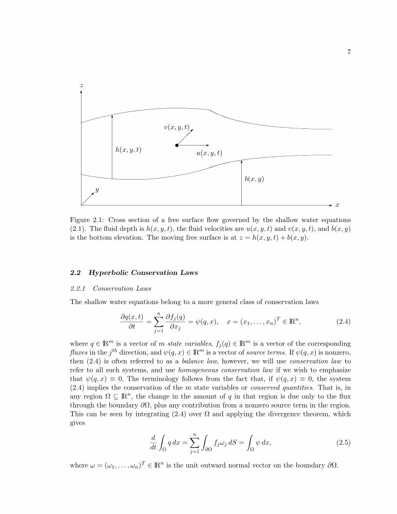
where g is the gravitational constant, h(x, y, t) is the nonnegative fluid depth, u(x, y, t) is thefluid velocity in the x-direction, v(x, y, t) is the fluid velocity in the y-direction and b(x, y) isthe elevation of the bottom surface (see Figure 2.1). The system (2.1) governs free surfaceflows where the fluid acceleration in the vertical z-direction is zero and horizontal velocitiesare uniform in the vertical direction. These simplifying assumptions will be discussed andthe equations (2.1) derived in Chapter 4. In this chapter we will confine our attention tosolutions to systems such as (2.1), and save any discussion regarding the relevance of theshallow water approximation until Chapter 4 and Chapter 5.

For theoretical examination, frequently it will be convenient to discuss the one dimen-sional form of the shallow water equations

ht + (hu)x = 0, (2.2a)

(hu)t + (hu2 +12gh2)x = −ghbx, (2.2b)

where subscripts denote partial derivatives (()t ≡ ∂∂t). If the bottom elevation is flat, bx ≡ 0,

(2.2) reduces to the homogeneous shallow water equations:

ht + (hu)x = 0, (2.3a)

(hu)t + (hu2 +12gh2)x = 0. (2.3b)

7

6

z

- xy

6

b(x, y)

6

h(x, y, t)-

tu(x, y, t)

v(x, y, t)

Figure 2.1: Cross section of a free surface flow governed by the shallow water equations(2.1). The fluid depth is h(x, y, t), the fluid velocities are u(x, y, t) and v(x, y, t), and b(x, y)is the bottom elevation. The moving free surface is at z = h(x, y, t) + b(x, y).

2.2 Hyperbolic Conservation Laws

2.2.1 Conservation Laws

The shallow water equations belong to a more general class of conservation laws

∂q(x, t)∂t

=n∑j=1

∂fj(q)∂xj

= ψ(q, x), x = (x1, . . . , xn)T ∈ lRn, (2.4)

where q ∈ lRm is a vector of m state variables, fj(q) ∈ lRm is a vector of the correspondingfluxes in the jth direction, and ψ(q, x) ∈ lRm is a vector of source terms. If ψ(q, x) is nonzero,then (2.4) is often referred to as a balance law, however, we will use conservation law torefer to all such systems, and use homogeneous conservation law if we wish to emphasizethat ψ(q, x) ≡ 0. The terminology follows from the fact that, if ψ(q, x) ≡ 0, the system(2.4) implies the conservation of the m state variables or conserved quantities. That is, inany region Ω ⊆ lRn, the change in the amount of q in that region is due only to the fluxthrough the boundary ∂Ω, plus any contribution from a nonzero source term in the region.This can be seen by integrating (2.4) over Ω and applying the divergence theorem, whichgives

d

dt

∫Ωq dx =

n∑j=1

∫∂Ωfjωj dS =

∫Ωψ dx, (2.5)

where ω = (ω1, . . . , ωn)T ∈ lRn is the unit outward normal vector on the boundary ∂Ω.

8

2.2.2 Hyperbolic Conservation Laws

The system (2.4) is said to be hyperbolic if the flux functions satisfy certain properties.

Definition 2.1. Hyperbolicity. Let∂fj∂q

denote the Jacobian matrix of the function fj(q), and consider the matrix

A(q, ω) =n∑j=1

ωj∂fj∂q

where ω = (ω1, . . . , ωn)T is a unit vector. The system (2.4) is hyperbolic, if A(q, ω) has mreal eigenvalues λp(q, ω), p = 1, . . . ,m, and m linearly independent eigenvectors rp(q, ω),p = 1, . . . ,m, for all ω ∈ lRn, |ω| = 1. Further, the system (2.4) is strictly hyperbolic at astate q0 if the eigenvalues λp(q0, ω), p = 1, . . . ,m, are distinct.

The integral conservation law (2.5) will also be referred to as hyperbolic, if the corre-sponding system of PDEs (2.4) is hyperbolic. Note that the matrix A(q, ω) is the Jacobian ofthe flux in the direction ω. The arbitrariness of ω implies that hyperbolicity is independentof any particular choice of coordinate directions.

The shallow water equations are hyperbolic conservation laws. As we will see, solutionsto hyperbolic conservation laws will share certain properties, and by identifying the shallowwater equations with this broader class of equations, we will be able to exploit the body oftheory and numerical methods previously developed for these mathematically challengingsystems.

2.3 Discontinuities and Weak Solutions

Although hyperbolic conservation laws were introduced as a system of PDEs (2.4) thatimplied the integral system (2.5), in most applications the integral system is derived fromfirst principles and is the more fundamental governing system. The two are equivalent ifthe solution is continuously differentiable, however, the integral system (2.5) admits non-smooth, even discontinuous solutions for which the PDEs are not defined in the classicalsense. We seek solutions to the more fundamental integral system, which can be shownto be equivalent to weak solutions to (2.4)—more generalized nonclassical solutions in thesense of distributions. See, for intstance, [22] for a general treatment of distribution theoryand generalized solutions to PDEs.

2.3.1 The Rankine-Hugoniot Jump Conditions

The weak solutions that arise in physical applications are characterized by regions of smoothvariation separated by propagating jump discontinuities. We can therefore isolate weaksolutions by requiring that they satisfy the PDEs where smooth, and meet appropriatejump conditions across discontinuities derived by the integral form. If we apply the integral

9

conservation law (2.5) to a region around a jump discontinuity, it is easy to derive (e.g.[67, 32]) the following condition:

|s|(q+ − q−

)=

n∑j=1

sj(fj(q+)− fj(q−)

), (2.6)

where |s| is the instantaneous speed of the propagating discontinuity, s is a unit vector in thedirection of the propagation, and the superscripts denote the limiting value of the solutionon either side of the discontinuity. The condition (2.6) on discontinuous solutions is knownas the Rankine-Hugoniot jump condition. It is easy to show that (2.6) is unaffected by asource term that is bounded in the neighborhood of the discontinuity.

For a one-dimensional system, (2.6) is simply

s [[q]] = [[f(q)]] , (2.7)

where s is the speed of the discontinuity, and [[·]] denotes the jump in the quantity acrossthe discontinuity.

2.3.2 Entropy Conditions

While uniqueness is guaranteed for smooth classical solutions to the hyperbolic PDEs (2.4),uniqueness of discontinuous solutions to the integral conservation laws (2.5) is not guaran-teed, and additional admissability conditions based on physical considerations are requiredto isolate the physically relevant solution. These admissability conditions are called entropyconditions, owing to the Euler equations of gas dynamics—a hyperbolic system for whichentropy plays this role. An entropy function ν(q) is an additional conserved quantity whenthe solution is smooth, obeying another conservation law

ν(q)t + ψ(q)x = 0, (2.8)

where ψ(q) is an entropy flux—some function based on physical considerations. For the shal-low water equations, ν(q) is the mechanical energy, ψ(q) is the energy flux, and (2.8) can beshown to be equivalent to the shallow water PDEs (2.2). For discontinuous solutions, (2.8)becomes an inequality based on the physical admissability considerations. For the shallowwater equations, mechanical energy must decrease in a region containing a discontinuity,and the equality in (2.8) is replaced by an inequality, ≤, for more general solutions.

An alternative formulation of entropy conditions can be found for systems satisfyingcertain mathematical properties, of which the shallow water equations belong. That formu-lation will be more convenient for our purposes, and will be discussed further below.

2.3.3 Steepening Waves

It should be realized that the admissability of discontinuous solutions to the integral formof hyperbolic conservation laws is not merely a mathematical technicality. The existenceof smooth initial conditions by no means implies that the solution to a hyperbolic systemwill remain smooth, and depending on the form of the flux function, various smooth initial

10

data leads to steepening waves—eventually leading to a shock discontinuity. Therefore, formost applications, the existence of discontinuous solutions cannot be ignored by merelyconsidering smooth initial data.

2.4 Linear and Quasilinear Hyperbolic Systems

2.4.1 One-Dimensional Linear Systems

Some basic properties of solutions to hyperbolic conservation laws are elucidated by con-sidering the simple linear homogeneous case in one dimension, where the flux f(q) = Aqimplies the system

qt +Aqx = 0. (2.9)

In order for (2.9) to be hyperbolic, the constant matrix A ∈ lRm×m must have real eigen-values λ1, . . . , λm, and a corresponding set of linearly independent eigenvectors r1, . . . , rm.Since A is therefore diagonalizable, (2.9) is equivalent to the diagonal system

wt + Λwx = 0, (2.10)

where w = R−1q, R is the matrix of eigenvectors, and Λ = R−1AR is the diagonal matrixof eigenvalues. Since (2.10) is a decoupled system of m scalar advection equations, we notethat the initial profile of each characteristic variable wp, p = 1, . . . ,m, is advected at theconstant speed of the corresponding eigenvalue λp. (For a review of the solution to scalaradvection equations, see for instance [67]). The characteristic curves of (2.9) in the x–t planeare therefore straight lines of unvarying slope, carrying the “weight” of each eigenvector atthe speed of an associated eigenvalue.

2.4.2 Quasilinear Hyperbolic Systems

In general f(q) is a nonlinear function of q, but we can write the one dimensional conserva-tion law

qt + f(q)x = 0, (2.11)

as a quasilinear system

qt + f ′(q)qx = 0, (2.12)

where f ′(q) denotes the Jacobian matrix of the flux. Although hyperbolicity implies thatf ′(q) is diagonalizable, the eigenvalues and eigenvectors are generally functions of q. Aswith linear systems, however, all solution information is carried at the local speed of theeigenvalues of f ′(q). The characteristics associated with a particular eigenpair λp, rp willbe referred to as the pth characteristic family or pth characteristic field.

The conservative system (2.12) belongs to a larger class of hyperbolic systems of PDEs

qt +B(q, x)qx = 0, (2.13)

11

where B(q, x) ∈ lRm×m is a nonlinear diagonalizable matrix with real eigenvalues. Ingeneral, however, B(q, x)qx need not be a full derivative of any function, and so (2.13)is not necessarily a conservation law. Nevertheless, many of the properties of solutions to(2.12) and the larger class of systems (2.13), are shared. For instance, the wave-like behaviorof solutions to hyperbolic conservation laws is due to the fact that information propagatesat the finite speed of the eigenvalues. This remains true for (2.13).

2.5 Riemann Problems

We will be interested in weak solutions to one-dimensional hyperbolic conservation laws,and hyperbolic systems generally, given a specific form of initial data that happens to betractable to analytical solution techniques. Consider the one-dimensional system

qt + f(q)x = 0, x ∈ lR, t > 0, (2.14a)

with piecewise constant initial conditions

q(x, 0) =

ql if x < 0,qr if x > 0.

(2.14b)

The initial value problem (2.14) is known as the Riemann problem.

2.5.1 Linear Waves

If f(q) happens to be linear, we know that the initial profile of each characteristic variable wp

translates at the speed of the corresponding eigenvalue λp. This implies that the solution to(2.14) in the linear case is a set of constant states separated bym discontinuities propagatingaway from the origin at the speed of the eigenvalues. The jump (q+ − q−) across the pth

discontinuity must be proportional to the pth eigenvector, since it represents the initialjump in the characteristic variable, wp, where q = Rw. The solution to the linear Riemannproblem can therefore be determined by decomposing the initial jump into the eigenvectorsrp of f ′(q) = A,

qr − ql =m∑p=1

αprp, (2.15)

and noting that each discontinuity αprp propagates at the speed λp. We will denote thediscontinuity Wp = αprp, and refer to it as the pth−wave. Note that each wave satisfies theRankine-Hugoniot conditions (2.7) for discontinuities since f(q) = Aq.

2.5.2 Nonlinear Waves

For the nonlinear case, the solution also consists of a set of transitions in each characteristicfamily that connect the states ql and qr. These transitions separate regions where thesolution is constant, however, the transitions are not necessarily discontinuous. Three typesof transitions can be distinguished: rarefactions, shock waves, and contact discontinuities.

12

A rarefaction is a type of smooth differentiable transitions in a particular characteristicfield, that if parameterized, is an integral curve of the associated eigenvector in phase space.That is, the solution satisfies q(x, t) = q(ξ(x, t)) throughout the wave, where

q′(ξ) = α(ξ)rp(ξ), (2.16)

for some function ξ(x, t), where α(ξ) is some scalar depending on the particular functionξ. A solution with such properties is known as a simple wave, of which, a rarefaction isone type arising in Riemann problems. Shock waves and contact discontinuities are bothdiscontinuities satisfying (2.7). In order to distinguish the two, the following definitions arerequired:

Definition 2.2. The pth characteristic field is called genuinely nonlinear if

∇λp(q) · rp(q) 6= 0, ∀q ∈ Ω. (2.17a)

Alternatively, the pth characteristic field is called linearly degenerate if

∇λp(q) · rp(q) ≡ 0, ∀q ∈ Ω. (2.17b)

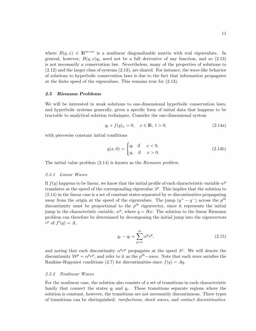
Shock waves are discontinuities in a genuinely nonlinear field. A contact discontinuityconversely, is a jump in a linearly degenerate field. If a field is linearly degenerate, the eigen-value would be unchanged through any simple wave satisfying (2.16), because of (2.17b).The field is similar to a linear field then, in the sense that the characteristic curves have aconstant slope through any transition that remains proportional to the pth eigenvector. Acontact discontinuity in the pth field may be thought of as a jump from one point to anotheron an integral curve of rp. In this case, s = λp(q+) = λp(q−), where s is the speed of thediscontinuity. For each of the three types of waves, the characteristics of the correspondingfield are shown in Figure 2.2.

It can be shown (e.g. [32]) that the Riemann problem (2.14) has a unique entropysatisfying weak solution if all of the m characteristic fields are either genuinely nonlinear orlinearly degenerate, provided that |qr− ql| is sufficiently small. Furthermore, the solution isa similarity solution depending only on (x/t), where (m+ 1) constant states are separatedby waves—shock waves, rarefactions or contact discontinuities. Solutions to a linear andnonlinear Riemann problem with m = 2 are depicted in Figure 2.3.

2.5.3 Entropy

For strictly hyperbolic conservation laws where each field is genuinely nonlinear, an alterna-tive formulation of the entropy condition holds that does not explicitly require an entropyfunction (2.8). This is known as the Lax entropy condition, and the following definition isborrowed from [67] .

Definition 2.3. Lax entropy condition. A discontinuity separating states ql and qr, prop-agating at speed s, satisfies the Lax entropy condition if there is an index p such that

λp(ql) > s > λp(qr), (2.18a)

13

(a) (b) (c)

x = 0

t

x = 0

t

x = 0

t

Figure 2.2: Characteristics of the three wave-types in Riemann solutions are shown in the x–t plane. (a) A rarefaction in the pth field: the p-characteristics emanating from x = 0 moveat a speed x/t. If the solution is parameterized through the rarefaction, it smoothly variesalong an integral curve of rp. (b) A shock in the pth field: the p-characteristic impinge on theshock according to the Lax entropy condition (Definition 2.3). (c) A contact discontinuityin the pth field: the discontinuity and p-characteristics on either side of the discontinuity allpropagate at the same speed.

so that p-characteristics are impinging on the discontinuity, while the other characteristicsare crossing the discontinuity,

λj(ql) < s and λj(qr) < s for j < p, (2.18b)

λj(ql) > s and λj(qr) > s for j > p, (2.18c)

where, in this definition, the eigenvalues are ordered so that λ1 < λ2 < · · · < λm in eachstate.

2.5.4 The Shallow Water Riemann Problem and Characteristic Structure

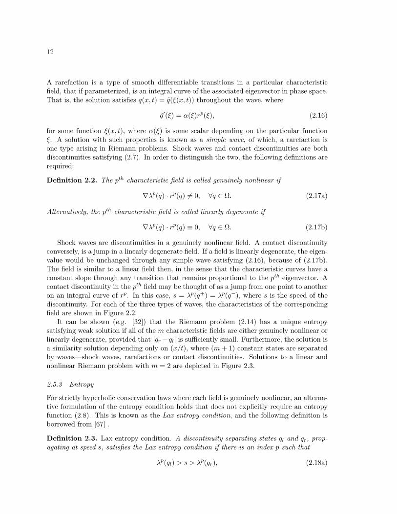
For the homogeneous shallow water equations in one dimension (2.3), we have

q =[hhu

], f(q) =

[hu

hu2 + 12gh

2

]. (2.19)

(The flux and the following quantities derived from it will frequently be denoted as functionsof the conserved variable q, but their formulas will be written in terms of the more familiarvariables, h and u.) The Jacobian matrix (differentiated with respect to q) for the flux is

f ′(q) =[

0 1−u2 + gh 2u

], (2.20)

which has eigenvalues

λ1(q) = u−√gh, λ2(q) = u+

√gh, (2.21)

14

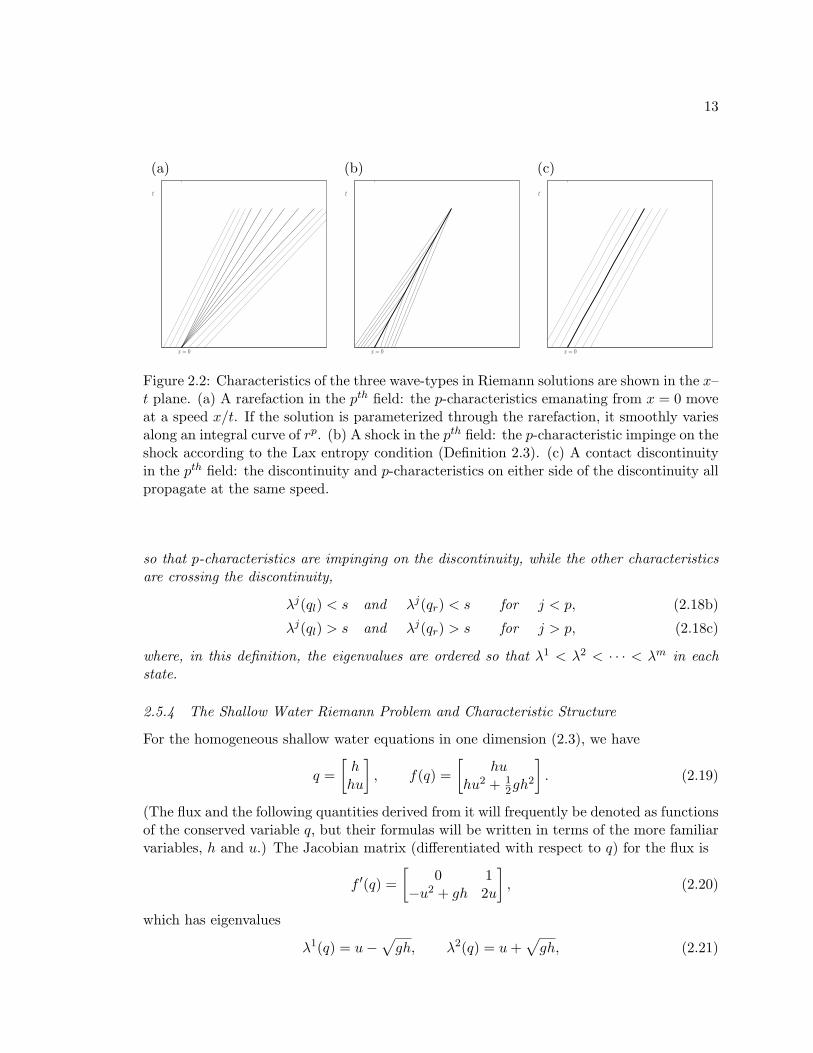
(a) (b)

t

ql qrq∗

W1= α1r1 W2

= α2r2

λ1 λ2

x = 0

s

qrql q∗

x = 0

t

λ1(q)

Figure 2.3: (a) The solution to a Riemann problem for a linear system in the x–t plane. Thesolution consists of m waves—each a jump discontinuity Wp proportional to the eigenvectorrp of A, moving at the speed of the corresponding eigenvalue λp. (b) An example of asolution to a nonlinear Riemann problem in the x–t plane showing each of the waves orcharacteristic transitions. The example shows 1-characteristics for a rarefaction in the firstfield, and shows a propagating discontinuity—a shock in the second field. In both (a) and(b) regions where the solution is constant are separated by the moving waves. For m = 2,there is a single constant middle state denoted q∗.

and corresponding eigenvectors

r1(q) =[

1λ1

], r2(q) =

[1λ2

]. (2.22)

It is easy to show that both characteristic fields are genuinely nonlinear. Therefore, theRiemann problem must consist of two waves—each wave being either a rarefaction or ashock—separating a single constant middle state from the adjacent state, ql or qr. Thesingle constant middle state will be denoted q∗, and the region it occupies in the x–t planewill occasionally be referred to as the middle region (see Figure 2.3). The unique entropysatisfying weak solution to the Riemann problem for the shallow water equations can bedetermined, though this entails nonlinear root finding. This will be described in more detailin Chapter 4 (see also [64, 101]). Several concepts that help elucidate this process will bebriefly introduced below.

It is possible to show that an integral curve in the phase plane of a genuinely nonlinearfield corresponds to a constant contour of a function of q (e.g. [64, 32]). These functionsare called Riemann invariants since the value of the function is invariant along an integralcurve. For the shallow water equations, the Riemann invariant of the first and second field

15

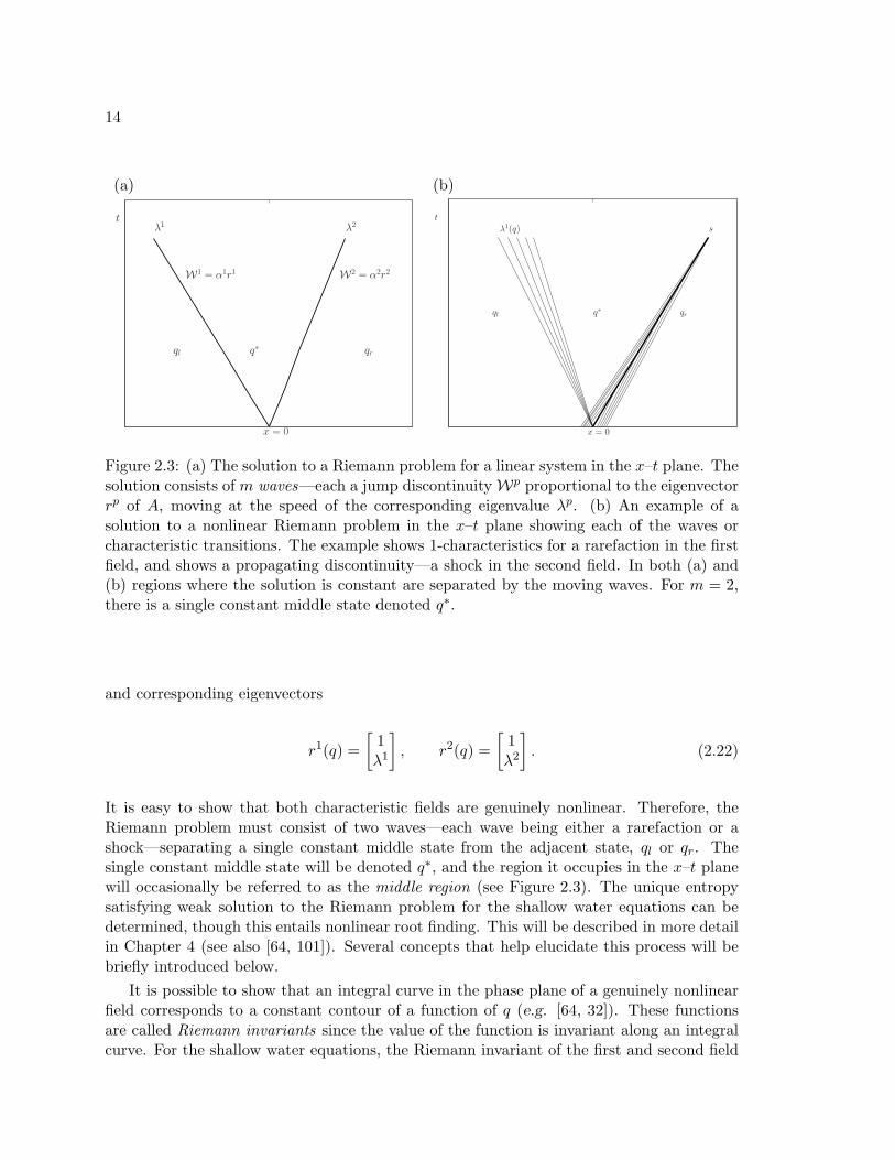
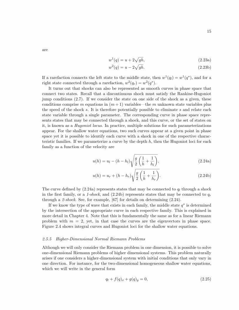
are

w1(q) = u+ 2√gh, (2.23a)

w2(q) = u− 2√gh. (2.23b)

If a rarefaction connects the left state to the middle state, then w1(ql) = w1(q∗), and for aright state connected through a rarefaction, w2(qr) = w2(q∗).

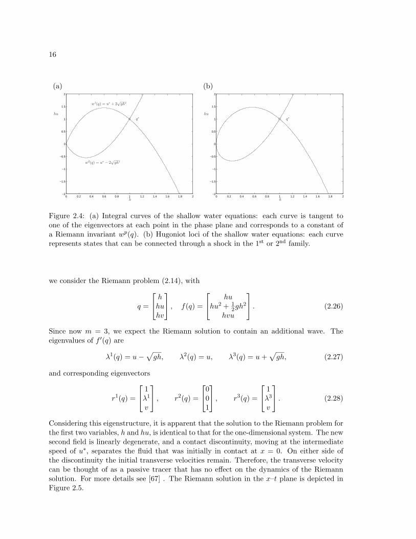
It turns out that shocks can also be represented as smooth curves in phase space thatconnect two states. Recall that a discontinuous shock must satisfy the Rankine-Hugoniotjump conditions (2.7). If we consider the state on one side of the shock as a given, theseconditions comprise m equations in (m+ 1) variables—the m unknown state variables plusthe speed of the shock s. It is therefore potentially possible to eliminate s and relate eachstate variable through a single parameter. The corresponding curve in phase space repre-sents states that may be connected through a shock, and this curve, or the set of states onit, is known as a Hugoniot locus. In practice, multiple solutions for such parameterizationsappear. For the shallow water equations, two such curves appear at a given point in phasespace yet it is possible to identify each curve with a shock in one of the respective charac-teristic families. If we parameterize a curve by the depth h, then the Hugoniot loci for eachfamily as a function of the velocity are

u(h) = ul − (h− hl)

√g

2

(1h

+1hl

), (2.24a)

u(h) = ur + (h− hr)

√g

2

(1h

+1hr

). (2.24b)

The curve defined by (2.24a) represents states that may be connected to ql through a shockin the first family, or a 1-shock, and (2.24b) represents states that may be connected to qrthrough a 2-shock. See, for example, [67] for details on determining (2.24).

If we know the type of wave that exists in each family, the middle state q∗ is determinedby the intersection of the appropriate curve in each respective family. This is explained inmore detail in Chapter 4. Note that this is fundamentally the same as for a linear Riemannproblem with m = 2, yet, in that case the curves are the eigenvectors in phase space.Figure 2.4 shows integral curves and Hugoniot loci for the shallow water equations.

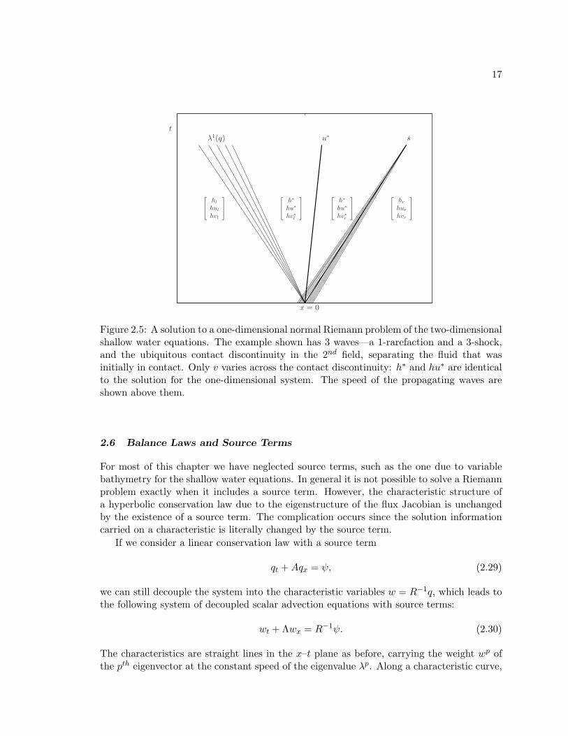
2.5.5 Higher-Dimensional Normal Riemann Problems

Although we will only consider the Riemann problem in one dimension, it is possible to solveone-dimensional Riemann problems of higher dimensional systems. This problem naturallyarises if one considers a higher-dimensional system with initial conditions that only vary inone direction. For instance, for the two-dimensional homogeneous shallow water equations,which we will write in the general form

qt + f(q)x + g(q)y = 0, (2.25)

16

(a) (b)

0 0.2 0.4 0.6 0.8 1 1.2 1.4 1.6 1.8 2−2

−1.5

−1

−0.5

0

0.5

1

1.5

2

q∗

h

hu

w2(q) = u∗ − 2√

gh∗

w1(q) = u∗ + 2√

gh∗

0 0.2 0.4 0.6 0.8 1 1.2 1.4 1.6 1.8 2−2

−1.5

−1

−0.5

0

0.5

1

1.5

2

q∗

h

hu

Figure 2.4: (a) Integral curves of the shallow water equations: each curve is tangent toone of the eigenvectors at each point in the phase plane and corresponds to a constant ofa Riemann invariant wp(q). (b) Hugoniot loci of the shallow water equations: each curverepresents states that can be connected through a shock in the 1st or 2nd family.

we consider the Riemann problem (2.14), with

q =

hhuhv

, f(q) =

huhu2 + 1

2gh2

hvu

. (2.26)

Since now m = 3, we expect the Riemann solution to contain an additional wave. Theeigenvalues of f ′(q) are

λ1(q) = u−√gh, λ2(q) = u, λ3(q) = u+

√gh, (2.27)

and corresponding eigenvectors

r1(q) =

1λ1

v

, r2(q) =

001

, r3(q) =

1λ3

v

. (2.28)

Considering this eigenstructure, it is apparent that the solution to the Riemann problem forthe first two variables, h and hu, is identical to that for the one-dimensional system. The newsecond field is linearly degenerate, and a contact discontinuity, moving at the intermediatespeed of u∗, separates the fluid that was initially in contact at x = 0. On either side ofthe discontinuity the initial transverse velocities remain. Therefore, the transverse velocitycan be thought of as a passive tracer that has no effect on the dynamics of the Riemannsolution. For more details see [67] . The Riemann solution in the x–t plane is depicted inFigure 2.5.

17

s

hr

hur

hvr

hl

hul

hvl

h∗

hu∗

hv∗r

h∗

hu∗

hv∗l

x = 0

t

λ1(q) u∗

Figure 2.5: A solution to a one-dimensional normal Riemann problem of the two-dimensionalshallow water equations. The example shown has 3 waves—a 1-rarefaction and a 3-shock,and the ubiquitous contact discontinuity in the 2nd field, separating the fluid that wasinitially in contact. Only v varies across the contact discontinuity: h∗ and hu∗ are identicalto the solution for the one-dimensional system. The speed of the propagating waves areshown above them.

2.6 Balance Laws and Source Terms

For most of this chapter we have neglected source terms, such as the one due to variablebathymetry for the shallow water equations. In general it is not possible to solve a Riemannproblem exactly when it includes a source term. However, the characteristic structure ofa hyperbolic conservation law due to the eigenstructure of the flux Jacobian is unchangedby the existence of a source term. The complication occurs since the solution informationcarried on a characteristic is literally changed by the source term.

If we consider a linear conservation law with a source term

qt +Aqx = ψ, (2.29)

we can still decouple the system into the characteristic variables w = R−1q, which leads tothe following system of decoupled scalar advection equations with source terms:

wt + Λwx = R−1ψ. (2.30)

The characteristics are straight lines in the x–t plane as before, carrying the weight wp ofthe pth eigenvector at the constant speed of the eigenvalue λp. Along a characteristic curve,

18

X(t) = x0 + λpt, each component obeys the ODE

d

dt(wp(X(t), t)) = (R−1ψ)p, (2.31)

suggesting that the decomposed source term is carried on characteristics as well. For in-stance, if the source term ψ happens to be proportional to an eigenvector rp, then it affectsonly the wp characteristic variable.

For a nonlinear system, the effect of the source term is considerably more complex sincethe eigenvalues and eigenvectors are functions of the solution. The solution to a Riemannproblem with a source term would not, in general, be a similarity solution—a function of(x/t) only—since the characteristics can curve with the changing eigenvalues. Similarly, ifthe source term is bounded, the instantaneous speed of a shock still obeys the Rankine-Hugoniot conditions, however, the value of the solution on either side of a shock can changedue to the source term, curving the shock in the x–t plane.

An alternative view of the effect of a source term is provided by considering a concen-trated point source. Suppose that the source term acts at a single point, ψ(q, x) = Ψδ(x),where δ(x) is the delta function defined by the functional

f(0) =∫f(x)δ(x) dx. (2.32)

By applying conservation to a vanishingly small neighborhood around x = 0, it is easy toshow (e.g. [67] ) that the flux must satisfy

f(q(0+, t))− f(q(0−, t)) = Ψ. (2.33)

Away from the concentrated source the conservation law is essentially homogeneous, sinceψ(q, x) = 0. The solution to a Riemann problem with a source term at the initial discon-tinuity is therefore a similarity solution. Like the homogeneous conservation law, a set ofwaves propagate away from the interface into regions with no source term, yet, a contactdiscontinuity remains at x = 0 where the flux obeys (2.33). This view will help elucidatenumerical methods where the source term is idealized as a point source ψ(q, x) = Ψ∆xδ(x),where ∆x is some interval that the point source “acts for.” That is, Ψ ≈ ψ(q(0, t), 0) sothat

∫ x2

x1ψ(q, x) dx ≈ Ψ∆x, where ∆x = (xr − xl).

19

Chapter 3

FINITE VOLUME METHODS AND WAVE PROPAGATIONALGORITHMS

This chapter gives an overview of a class of numerical methods developed for hyperbolicconservation laws (2.4). Originally, these methods were developed largely in the contextof solving the Euler equations of compressible gas dynamics, however, they are generallyapplicable to other systems such as the shallow water equations. Additionally, we willconsider wave propagation algorithms—finite volume methods that are applicable to moregeneral hyperbolic systems (2.13). Ultimately, as will be described in this and later chapters,the more general wave propagation algorithms will be used to solve the shallow waterequations. This chapter describes the basic methods—modifications specific to tsunamimodeling will be taken up in later chapters.

3.1 Finite Volume Methods for Conservation Laws

For numerically solving systems that obey integral conservation laws, finite volume methodsprovide a natural intuitive approach. In this approach, the numerical solution can beviewed as a piecewise constant function in space rather than a set of values at discretepoints. The spatial domain is divided into a set of grid cells where the numerical solutionhas a given value at each time step. In one dimension, the grid cells are simply intervalsCi = [xi−1/2, xi+1/2] of length ∆x, around the point xi = x0+i∆x, where xi±1/2 = xi± 1

2∆x,i ∈ Zc ⊆ Z. (For simplicity we will assume that the intervals are all of equal length∆x, however, this is not strictly necessary.) The numerical solution Qni ∈ lRm is then anapproximation to the average value of the true solution in the grid cell

Qni ≈1

∆x

∫Ci

q(x, tn) dx. (3.1)

(For analysis of smooth solutions, note that Qni ≈ q(xi, tn).) If we wish to approximate ahomogeneous conservation law, the numerical solution can be updated from time tn to tn+1,with ∆t = tn+1 − tn, by the explicit flux-differencing scheme

Qn+1i = Qni −

∆t∆x

[Fni+1/2 − Fni−1/2

], (3.2)

where Fni±1/2 are the numerical fluxes—approximations to the fluxes at the grid cell bound-aries. Note that (3.2) is a direct approximation to the integral conservation law applied to

20

the domain Ci, which integrated from time tn to tn+1 and divided by ∆x gives

1∆x

∫Ci

q(x, tn+1) dx =1

∆x

∫Ci

q(x, tn) dx

− 1∆x

[∫ tn+1

tnf(q(xi+1/2, t)) dt−

∫ tn+1

tnf(q(xi−1/2, t)) dt

]. (3.3)

Considering (3.1) and (3.3), note that the numerical fluxes in (3.2) should be approximationsto the time averaged fluxes at the cell boundaries:

Fni±1/2 ≈1

∆t

∫ tn+1

tnf(q(xi±1/2, t)) dt. (3.4)

Because (3.3) is exact, the accuracy and stability of the numerical method (3.2) is deter-mined by the approximation (3.4). Developing an explicit flux differencing scheme of theform (3.2), therefore, entails developing consistent and stable numerical fluxes.

Note that (3.2) is a conservative numerical scheme regardless of the form of Fni±1/2.That is, the numerical solution is conserved on the computing domain (aside from anycontribution from the boundaries), since the same Fni−1/2 is used to update Qni−1 and Qni .This implies that whatever quantity enters one grid cell must leave another, as with thetrue conservation law. It turns out that numerical conservation is a necessary condition forconverging to the correct discontinuous solutions to conservation laws [47].

3.2 Godunov-Type Methods

A class of methods that provide a stable and consistent approximation to the numericalfluxes (3.4), are the Godunov-type methods. The original Godunov method [33], is a first-order upwind-type scheme, where Riemann problems are solved at each grid cell interfacebefore each time step to determine the numerical flux for that time step. That is, at timetn, ∀i ∈ Zc, we solve the Riemann problem (2.14), with data ql = Qni−1 and qr = Qni . If wedenote the similarity solution to the Riemann problem, described in the previous chapter,as q(x/t, ql, qr), then our numerical flux Fni−1/2 becomes f(q(0, Qni−1, Q

ni ))—the actual flux

function evaluated with the solution to the Riemann problem at x = 0. At first glance,solving the Riemann problem seems like an overly involved procedure for estimating theflux (3.4), however, it turns out that it provides several essential properties. First, theexplicit time update in (3.2) requires proper upwinding of the flux estimate for stability.For a first order method, the Riemann solution provides the proper upwinding, even whenthere are m characteristic curves. Second, the Godunov method converges to entropy sat-isfying discontinous weak solutions, provided that the Riemann solutions satisfy entropyconditions. The standard Godunov method is only first order accurate but standard sec-ond order methods, based on the validity of Taylor series, break down near discontinuities.If fact, it can be shown that no linear second order method can converge to discontinu-ous solutions in general (where linearity is in the sense of the abstract updating functionQn+1i = L(∆x,∆t, Qn1 , . . . , Q

ni , . . . )). See, for example, [32, 67, 100] for a full discussion of

21

these topics. Later in this chapter we will discuss the extension of the standard Godunovmethod to higher order methods for smooth solutions that maintain the ability to convergeto discontinuities.

In practice, it is often sufficient to approximate the solution to the Riemann problem,and various approximate Riemann solvers have been developed specifically for Godunov-type methods. Some standard approaches will be discussed in the next section.

3.3 Approximate Riemann Solvers

Approximate Riemann solvers are typically based on using a solution to some related linearproblem at each grid cell interface that approximates the true nonlinear Riemann solution.Recall that a solution to a linear Riemann problem consists of a set of discontinuities orwaves propagating at speeds equal to the eigenvalues of the constant Jacobian. All of theapproximate solvers discussed in this section will be of that same basic form. That is, theapproximate solutions consist of a set ofMw waves,Wp ∈ lRm, propagating at correspondingspeeds sp, p = 1, . . . ,Mw, where

qr − ql =Mw∑p=1

Wp. (3.5)

The new notation Mw is used for the number of waves, and sp for the speeds, since, for anapproximate solution, it is not strictly necessary that Mw = m, nor that sp correspond toactual eigenvalues λp of some Jacobian.

One approach for creating an approximating linear solution is to use a local lineariza-tion of the Jacobian, where f ′(q) is replaced with a constant matrix A(ql, qr). The resultinglinear Riemann problem is then solved to determine the numerical flux. In order to main-tain hyperbolicity, A(ql, qr) must have real eigenvalues and a full set of linear independenteigenvectors. Additionally, it must be consistent in the following sense: A(ql, qr) → f ′(q),as ql, qr → q.

If the approximate solution is conservative, that is, if it obeys the conservation law whenapplied to a region surrounding the Riemann solution, it must satisfy

f(qr)− f(ql) =Mw∑p=1

spWp. (3.6)

The right hand side represents the time rate of change of the solution due to the movingjump discontinuities Wp, and the left hand side represents the flux evaluated at the far sidesof the changing region. Not all linearizations will satisfy (3.6).

3.3.1 The Roe Solver

A particular linearization that is endowed with several nice properties is the Roe lineariza-tion, or the Roe solver. This was originally developed for the Euler equations by Roe [82],but it has since been extended to the shallow water equations. The Roe solver is based

22

on evaluating the flux Jacobian f ′(q) with a special average of qr and ql in the Riemannproblem. If we denote this matrix A, we have

A(ql, qr) = f ′(q(ql, qr)), (3.7)

where q(ql, qr) denotes the special Roe average of ql and qr. Because the Roe matrix isdetermined by evaluating the true flux Jacobian with a valid state q, all of the essentialhyperbolic eigenstructure is maintained. The essential and unique property of the averageq is that the resulting linear Riemann solution is conservative with respect to the originalflux. That is, the following property is satisfied:

f(qr)− f(ql) = A(ql, qr) (qr − ql) . (3.8)

By considering a decomposition of (qr−ql) into the eigenvectors of A(ql, qr), it is easy to seethat if (3.8) is satisfied, the solution to a linear Riemann problem with Jacobian A satisfiesthe conservation condition (3.6). The actual Roe average q(qr, ql) depends on the particularsystem of equations. For the shallow water equations,

h(ql, qr) =12

(hl + hr) , (3.9a)

u(ql, qr) =ul√hl + ur

√hr√

hl +√hr

, (3.9b)

where, as usual, the formulas have been written in terms of the more familiar variables hand u rather than q. Roe averages and the functions evaluated with them will be denotedwith a hat throughout this thesis.

A beneficial feature of the Roe solver is the approximate solution that it produces in theneighborhood of a shock. Suppose that the true solution to the Riemann problem is a singleshock wave propagating at speed s satisfying the Rankine-Hugoniot conditions. The Roesolver produces the exact solution in this case, following from its conservative properties:

s(qr − ql) = f(qr)− f(ql) = A(ql, qr)(qr − ql). (3.10)

The first equality in (3.10) is the Rankine-Hugoniot condition governing the true solution,and the second equality follows from (3.8). Recall that the solution to a linear problemcan be determined by decomposing the initial jump (qr − ql) into the eigenvectors of theJacobian and translating the resulting waves at the speed of the corresponding eigenvalues.Since (3.10) implies that (qr − ql) is an eigenvector of A(ql, qr) with eigenvalue s, clearlythe Roe solver produces the exact solution in this case. This can also be interpreted in thefollowing way: if the data ql and qr lie on the same Hugoniot locus of the pth characteristicfamily, the vector (qr − ql) is the eigenvector rp of A(ql, qr).

3.3.2 The HLL and HLLE solvers

The HLL solver, introduced by Harten, Lax and Van Leer [42], provides a simple con-servative alternative to the Roe linearization. The HLL solver does not use an explicitlinearization of the Jacobian, but rather constructs a conservative solution by requiring

23

that two discontinuities propagate at predetermined speeds, s1 and s2, s2 > s1, where thespeeds are based somehow on ql and qr. (The solver actually uses two speeds even whenthe system has m > 2 equations.) The middle state q∗ between the two discontinuities isthen determined by applying the conservation law to the region

s1(q∗ − ql) + s2(qr − q∗) = f(qr)− f(ql), (3.11a)

⇒q∗ =1

s1 − s2(s1ql − s2qr + f(qr)− f(ql)

). (3.11b)

The properties of the HLL solver are strongly tied to the pre-chosen speeds s1 and s2. Forthe shallow water equations, where m = 2, if s1 and s2 correspond to the Roe eigenvalues—the eigenvalues of f ′(q) evaluated at q—then the HLL solver is identical to the Roe solver,which follows from conservation.

The HLLE solver is an HLL type of solver that arises when a particular choice of speedsare used:

s1 = minp

min(λp(ql), λp(ql, qr)), (3.12a)

s2 = maxp

max(λp(qr), λp(ql, qr)), (3.12b)

where λ(ql, qr)p are the Roe eigenvalues, or the Roe speeds. The speeds (3.12) were advocatedby Einfeldt [20], and we will refer to them as the Einfeldt speeds, and denote them s1E ands2E . For the shallow water equations, it is easy to show that (3.13) is simply

s1E = min(λ1(ql), λ1(ql, qr)), (3.13a)

s2E = max(λ2(qr), λ2(ql, qr)). (3.13b)

The Einfeldt speeds endow the approximate solver for the shallow water equations withsome special properties that will be discussed further below and in Section 3.5. See also[20, 21].

3.3.3 Entropy Fixes

As mentioned previously, the Godunov-type methods converge to the correct entropy satis-fying discontinuous solutions, provided that the Riemann solutions are the correct entropysatisfying weak solutions. Since approximate Riemann solvers are discontinuous, even whenthe true solution is a smooth rarefaction, they can generate convergence to discontinuousentropy violating solutions. This well known problem occurs when the true solution to aRiemann problem contains a transonic rarefaction—a rarefaction in the pth field where λp

passes through zero. In this case the true solution has a wave spreading out in both direc-tions. Since an approximate solver uses a single discontinuity to represent this rarefaction,it allows convergence to the pathological stationary expansion shock—a stationary discon-tinuity at a cell interface that violates entropy. The Roe solver is prone to this problem,however, numerous entropy fixes have been developed for the Roe solver (e.g. [19, 40, 41]).

The HLLE method provides a natural fix to this problem, since, in the case of a transonicrarefaction, the speeds (3.12) bound the true speeds of the spreading rarefaction.

24

3.4 Wave Propagation Algorithms

The standard Godunov-methods are flux differencing methods (3.2), where exact or approx-imate solvers are used to determine a numerical flux (3.4), sometimes called an interfaceflux. These methods are conservative regardless of the form of the approximate Riemannsolution. Alternatively, the structure of an approximate Riemann solution can be used di-rectly to update the numerical solution. That is, the effect of moving waves Wp ∈ lRm

can be directly re-averaged onto the computational grid cells. This is the idea behind thewave propagation algorithms, such as those developed by LeVeque [65, 67]. For instance,an approximate Riemann solution at xi−1/2 with data ql = Qi−1 and qr = Qi, produces aset of waves:

Qi −Qi−1 =Mw∑p=1

Wpi−1/2, (3.14)

and a corresponding set of speeds spi−1/2, p = 1, . . . ,Mw. If these waves are re-averagedonto the adjacent grid cells, they produce a change of the average value to the right

Qn+1i −Qni = −∆t

∆x

∑np: sp

i−1/2>0o s

pi−1/2W

pi−1/2, (3.15)

and to the left

Qn+1i−1 −Qni−1 = −∆t

∆x

∑np: sp

i−1/2<0o s

pi−1/2W

pi−1/2. (3.16)

The net effect of the two Riemann problems on the boundaries of Ci is then

Qn+1i = Qni −

∆t∆x

∑np: sp

i−1/2>0o s

pi−1/2W

pi−1/2 +

∑np: sp

i+1/2<0o s

pi+1/2W

pi+1/2

. (3.17)

Adopting the notation from [67] , we will denote the sum in (3.15) as A+∆Qi−1/2 and thesum in (3.16) as A−∆Qi−1/2, and refer to them as fluctuations. The update (3.17) can thenbe written as

Qn+1i = Qni −

∆t∆x

(A+∆Qi−1/2 +A−∆Qi+1/2

). (3.18)

The wave propagation method is more generally applicable than the flux differencingapproach (3.2), since (3.18) can be applied to non-conservative hyperbolic systems of theform (2.13). In fact, (3.18) is a generally valid approach even when the Riemann solution hasa discontinuity at x = 0, or in the case of the numerical update, at a cell interface. If (3.18)is used for a conservation law, the following property is required to maintain conservation

f(Qi)− f(Qi−1) = A−∆Qi−1/2 +A+∆Qi−1/2. (3.19)

25

Note that if approximate solvers of the form described in Section 3.3 are used, (3.19) isequivalent to the requirement

f(Qi)− f(Qi−1) =Mw∑p=1

spi−1/2Wpi−1/2, (3.20)

which is equivalent to (3.6)—the condition that an approximate solution obeys conservation.

3.4.1 The f-wave Method

Decomposing the solution at a grid cell interface (3.14), and then requiring (3.20), suggests asimpler approach where the jump in the flux is simply decomposed into some set of vectors,

f(Qi)− f(Qi−1) =Mw∑p=1

Zpi−1/2, (3.21)

where Zpi−1/2 ∈ lRm is called an f-wave, since it carries the same dimension as the flux, likespi−1/2W

pi−1/2 (see [6]). As before, some set of speeds spi−1/2, p = 1, . . . ,Mw are associated

with the waves. The fluctuations can then be defined by

A−∆Qi−1/2 =∑

np: sp

i−1/2<0oZ

pi−1/2, (3.22a)

A+∆Qi−1/2 =∑

np: sp

i−1/2>0oZ

pi−1/2. (3.22b)

If all of the speeds are nonzero, decomposing the flux into any set of vectors will maintainconservation since, by (3.21) and (3.22), (3.19) is automatically satisfied. However, for con-sistency, as with the solution the flux should typically be decomposed into the eigenvectorsof the Jacobian. This follows from the fact that through any rarefaction of the pth family,f(q)x = f ′(q)qx = λprp. Additionally, across a shock in the pth family, [[f(q)]] = s [[q]].Note that if the Roe eigenvectors and speeds are used, the f -wave approach is the same asthe standard Roe solver, and each flux wave is exactly Zpi−1/2 = λp(Qi−1, Qi)Wp

i−1/2, wherethe waves Wp

i−1/2 are defined by a Roe decomposition of (Qi−Qi−1). This follows from theconservative property of the Roe solver (3.8).

In general, in order to ensure conservation, special measures have to be taken if one ofthe speeds spi−1/2 happens to be zero, such as splitting the wave into two waves moving ineither direction. However, this is not the case if Zpi−1/2 is also zero. If a flux wave Zpi−1/2

is nonzero, and it is stationary, spi−1/2 = 0, this represents a jump in the flux that does notchange the solution. For certain systems, such as systems with a source term, this may bedesired and in fact we will exploit this property in Chapter 6.

26

3.4.2 The CFL Condition

Recall that the CFL condition is a necessary condition for stability, and it requires thatthe numerical domain of dependence include the true domain of dependence. Since thewave propagation method uses the adjacent values to any grid cell to determine an explicitnumerical update, it is required that the time step satisfy

maxp(|spi−1/2|)∆t∆x

≤ 1, (3.23)

∀i ∈ Zc. Recall that the left hand side of (3.23) is the Courant number.

3.5 Depth Positivity and Vacuum States

For some applications, certain properties might be desired in the approximate Riemannsolution that are guaranteed in a true weak solution to the Riemann problem, such aspositivity of one of the conserved variables. For the shallow water equations, the depthsatisfies h ≥ 0, and it might be desired that approximate Riemann solution always reflectthis. However, the appearance of nonphysical negative values for the depth in the shallowwater equations as well as the density in the Euler equations of gas dynamics, is a wellknown problem. This problem is sometimes called the vacuum state problem, named fromthe latter application.

3.5.1 The Roe Solver

Unfortunately the Roe solver fails to maintain positivity of the depth h for the shallow waterequations. (This same difficulty is encountered for the density in the Euler equations.) Sincethe Roe decomposition for the shallow water equations

qr − ql =2∑p=1

αprp =2∑p=1

Wp (3.24)

corresponds to two discontinuities on either side of a constant middle state q∗, the singlemiddle state depth

h∗ = hl + α1(r1)1 = hr − α2(r2)1 (3.25)

corresponds to the intersection of the vectors r1 and r2 in phase space. In general, this isnot necessarilly positive—particularly if the initial data induces large rarefactions, such aswhen hur >> hul. This type of Riemann problem will be described in detail in Chapter 4.Figure 3.1 compares the approximate middle states for the Roe and HLLE solver—theintersection of constant vectors—with the true middle state—the intersection of the twointegral curves.

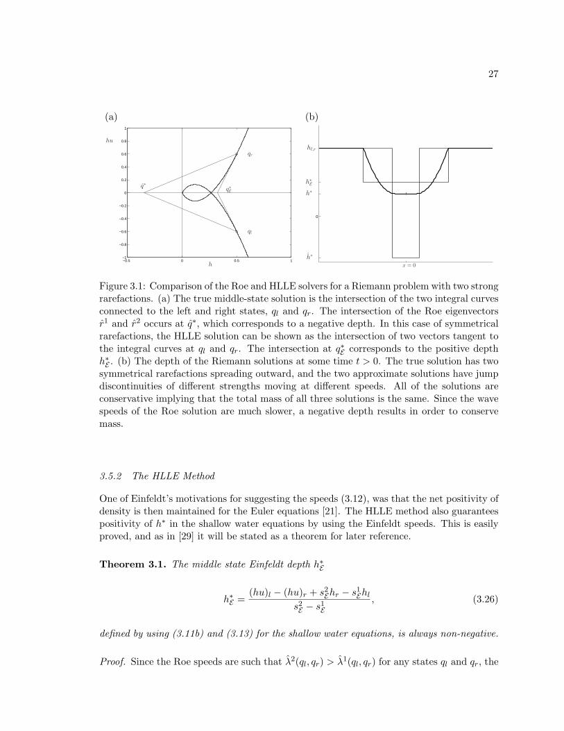
27

(a) (b)

−0.5 0 0.5 1−1

−0.8

−0.6

−0.4

−0.2

0

0.2

0.4

0.6

0.8

1

h

hu

qr

ql

q∗q∗E

0

hl,r

h∗E

h∗

h∗

x = 0

Figure 3.1: Comparison of the Roe and HLLE solvers for a Riemann problem with two strongrarefactions. (a) The true middle-state solution is the intersection of the two integral curvesconnected to the left and right states, ql and qr. The intersection of the Roe eigenvectorsr1 and r2 occurs at q∗, which corresponds to a negative depth. In this case of symmetricalrarefactions, the HLLE solution can be shown as the intersection of two vectors tangent tothe integral curves at ql and qr. The intersection at q∗E corresponds to the positive depthh∗E . (b) The depth of the Riemann solutions at some time t > 0. The true solution has twosymmetrical rarefactions spreading outward, and the two approximate solutions have jumpdiscontinuities of different strengths moving at different speeds. All of the solutions areconservative implying that the total mass of all three solutions is the same. Since the wavespeeds of the Roe solution are much slower, a negative depth results in order to conservemass.

3.5.2 The HLLE Method

One of Einfeldt’s motivations for suggesting the speeds (3.12), was that the net positivity ofdensity is then maintained for the Euler equations [21]. The HLLE method also guaranteespositivity of h∗ in the shallow water equations by using the Einfeldt speeds. This is easilyproved, and as in [29] it will be stated as a theorem for later reference.

Theorem 3.1. The middle state Einfeldt depth h∗E

h∗E =(hu)l − (hu)r + s2Ehr − s1Ehl

s2E − s1E, (3.26)

defined by using (3.11b) and (3.13) for the shallow water equations, is always non-negative.

Proof. Since the Roe speeds are such that λ2(ql, qr) > λ1(ql, qr) for any states ql and qr, the

28

denominator of (3.26) is always positive. For the numerator,

h∗E = (hu)l − (hu)r + s2Ehr − s1Ehl

≥ hlul − hrur + (ur +√ghr)hr − (ul −

√ghl)hl

= hr√ghr + hl

√ghl

≥ 0. (3.27)

Theorem 3.1 is intuitively clear if one considers the nature of the Einfeldt speeds. Thesespeeds are intended to bound the maximum and minimum speeds of waves arising out of thetrue Riemann solution. If the true Riemann solution maintains positivity of h for all (x/t),and it is replaced by a single constant state extending beyond the lower and upper values of(x/t) where the true solution varies—conservation ensures that the approximate solution isalso nonnegative. In fact, note from the proof of Theorem 3.1, that if the Eindeldt speedswere replaced by speeds sE1,2 that bound them from below and above:

sE1 ≤ s1E < s2E ≤ sE

2, (3.28)

then positivity would still be maintained.

3.5.3 The f-wave Method

In the f -wave approach, the flux, not the solution is not decomposed into waves. A middlestate solution q∗ is therefore not explicitly constructed since the jumps across the wavesZp do not correspond directly to jumps in q. However, for the shallow water equations,if one considers the numerical effect of the f -waves in defining the fluctuations (3.22), itis possible to define what we will call the effective middle state depth(s). That is, in thestandard decomposition of the solution, one has

h∗ = hl + (W1)1 = hr − (W2)1. (3.29)

The fluctuations that update the solution are then constructed by multiplying the wavesWp by the corresponding speed sp. In the f -wave approach, the fluctuations are definedby using Zp directly and these are associated with a speed sp. Note that if we decomposedthe flux directly, and then defined the fluctuations in the standard way, using Wp = Zp/sp,this would produce exactly the same numerical result as if Wp, representing jumps in thesolution, were determined by some other means.

Definition 3.1. Effective middle-state depths. If the fluctuations used in (3.18) are definedby a decomposition of the (shallow water) flux according to (3.22), then the effective middlestate depths are given by

h∗l = hl +(Z1)1

s1, (3.30a)

h∗r = hr −(Z2)1

s2. (3.30b)

29

More generally, given any wave-type approximate Riemann solver based on a flux decompo-sition, if the resulting numerical update is equivalent to that from a wave-type solver basedon a solution decomposition, the middle-state depths of the latter will be referred to as theeffective middle-state depths of the former.

In general, h∗r 6= h∗l , and for the f -wave approach, one may imagine a jump in the solutionat the cell interface, even if it is not explicitly constructed. (If the Roe eigenstructure isused, it is easy to show that h∗l = h∗r , so a jump at the cell interface is due to a deviationfrom the Roe eigenstructure.) If two middle states were explicitly constructed using (3.30),and the fluctuations were defined in the standard way, the update to the mass equationwould be identical to that of the f -wave decomposition.

Considering the positive preserving properties of the HLLE solver, it might seem that byusing some set of vectors with corresponding speeds equivalent to the Einfeldt speeds, thatpositivity of the f -wave method should be maintained based on conservation. However, thisis not the case since two effective middle state depths exist. It can be shown that the sum

s2Eh∗r − s1Eh

∗l , (3.31)

representing the net mass (divided by ∆t) of the Riemann solution between the two waveswould be positive for such a method. However, there is no guarantee in general that bothh∗l and h∗r are positive with the f -wave method.

3.5.4 Depth-Positive-Definite Riemann Solvers

We will summarize some of these ideas as a definition for later reference.

Definition 3.2. Depth-positive-definite Riemann Solvers. An approximate Riemann solverfor the shallow water equations with initial data hl, hr ≥ 0, that produces only nonnegativemiddle states, or effective middle states as defined by Definition 3.1, will be referred to asa depth-positive-definite Riemann solver.

It might also simply be said that the Riemann solver maintains positivity of the solution.It should be noted that using a depth positive definite Riemann solver is not the onlyrequirement for maintaining a nonnegative numerical solution. However, if the first orderupdate (3.18) is used in one dimension, and if the Courant number is restricted to 1/2 (1/4in two dimensions), it is sufficient. An additional fix is discussed in Section 3.9 if theserestrictions are not met.

3.6 Numerical Treatment of Source Terms

3.6.1 The Fractional Step Method

The numerical methods described so far have been based on solving a homogeneous conser-vation law. When a source term exists, the numerical method described for homogeneousconservation laws can be implemented unaltered, by incorporating the source term with a

30

separate integration step. This is called the fractional step method, or fractional stepping.The idea is to first solve the homogeneous conservation law

qt + f(q)x = 0, (3.32)

followed by an integration of the set of ODEs

qt = ψ(q, x) (3.33)

in each time step. The effect of alternating between these two steps incorporates the sourceterm. Accuracy of the individual methods can be inherited by the overall method (yet onlyup to second order, see [67] ) given specific formulations of the order and size of the timesteps (see Strang [88]).

The popularity of this approach is due to the fact that it is very simple and is veryrobust for many applications. The approach fails for applications where there is a prevalentsteady state that exists due to a nontrivial balance f(q)x ≈ ψ. In this case it is well known(see, for instance, [66, 6]) that fractional stepping fails to preserve the steady state, orresolve small deviations to it. This is quite intuitive, since if f(q)x ≈ ψ(q, x), and bothterms are large, the distinct steps for (3.32) and (3.33) must nearly and precisely undo oneanother, while resolving the small deviation. This situation is precisely what occurs withthe shallow water equations, where the “lake at rest” steady state over variable bathymetryis due to a nontrivial balance 1

2g(h2)x = −ghbx. This situation is exacerbated for tsunami

modeling, where the tsunami is actually a tiny, nearly infinitesimal deviation, consideringthe background steady state. This will be discussed in more detail in Chapter 5.

3.6.2 An f-wave Approach to Source Terms

The wave propagation methodology of LeVeque uses the waves arising from a Riemannsolver to directly update the solution. This same methodology can be applied to sourceterms as well; rather than treating source and flux terms separately, the effect of the sourceterm can be added directly to the updating waves in the fluctuations A±∆Q. This is theapproach suggested by Bale et al in [6]. This is accomplished, and is consistent with theoriginal conservation law, if the source term is subtracted from the flux difference beforeperforming the decomposition

f(Qi)− f(Qi−1)−∆xΨi−1/2 =Mw∑p=1

Zpi−1/2, (3.34)

where Ψi−1/2∆x is some approximation to∫ xi+1

xi−1ψ(q, x) dx. The fluctuations at grid cell

interfaces are then defined in the standard way (3.22), and the standard updating formula(3.18) can be used. If the source term is interpreted as a point source at the grid cellinterface, ψ(q, x) = Ψi−1/2∆xδ(x − xi−1/2), equation (3.34) amounts to subtracting thejump in the flux at the grid cell interface

f(q(x+i−1/2, t))− f(q(x−i−1/2, t)) = ∆xΨi−1/2 (3.35)

31

from the flux difference before decomposing into the propagating waves. If the Riemannproblem arises near a steady state where f(q)x ≈ ψ(q, x), then

f(Qi)− f(Qi−1)∆x

≈ Ψi−1/2, (3.36)

and nonzero waves in the decomposition (3.34) will be due to the deviation from the steadystate.

Equation (3.34) is said to upwind the source term, in the sense that the source term isdecomposed into the eigenvectors of the Jacobian and propagated at the wave speeds. Thisapproximates the true solution, as was pointed out for linear problems in Section 2.6. Infact, this form of upwinding has been commonly advocated (e.g. [83, 52]).

3.7 High Resolution Methods

The Godunov-type methods, as described so far, converge to discontinuous entropy satis-fying weak solutions, however, they are only first-order accurate and numerically diffusive.Various second-order methods, such as the Lax-Wendroff method, can be derived based onTaylor series expansions of the PDEs—requiring smoothness of the solution. These methodsnot only fail to be second-order accurate near discontinuities, they exhibit large spuriousoscillations near such features and are overly dispersive in general near steep gradients—problematic since hyperbolic equations typically exhibit steepening. This problem is circum-vented by the high-resolution methods—nonlinear methods that use standard second-orderformulas where the solution is smooth yet resort to the first-order Godunov methods nearshocks or steep gradients. This is accomplished by adding second-order corrections to thefirst-order method, together with the use of a limiter function φ that measures the localsmoothness of the solution.

The wave propagation algorithm (3.18) can be extended to a second-order accuratemethod

Qn+1i = Qni −

∆t∆x

(A+∆Qi−1/2 +A−∆Qi+1/2

)+

∆t∆x

(Fi+1/2 + Fi−1/2), (3.37)

where Fi±1/2 are limited second-order correction fluxes. These corrections can be definedin terms of the first-order waves,

Fi−1/2 =12

Mw∑p=1

|spi−1/2|(

1− ∆t∆x

|spi−1/2|)Wpi−1/2, (3.38)

where Wpi−1/2 = φWp

i−1/2 is a limited wave. For the f -wave approach, the correspondingcorrection flux must be

Fi−1/2 =12

Mw∑p=1

sgn(spi−1/2)(

1− ∆t∆x

|spi−1/2|)Zpi−1/2, (3.39)

where Zpi−1/2 = φZpi−1/2. If the limiters are absent (or φ=1), (3.37) is an extension of thesecond-order Lax-Wendroff method for systems (see [63, 67] for details). Note that in the

32

case of a source term, if the f -waves are defined by (3.34), then it is the deviations fromthe steady state that get limited.

Limiter functions interpret the smoothness of the solution by comparing the jump in thesolution in neighboring grid cells, and in the case of a potential shock, limit the waves in(3.38) or (3.39). Ideally, the limiter functions should isolate when a steep gradient or shockexists in one characteristic family and limit that corresponding wave. This is accomplishedby comparing the wave Wp

i−1/2 with WpI−1/2 where

I =

i− 1 if spi−1/2 > 0,

i+ 1 if spi−1/2 < 0.(3.40)

Some variable θ that measures the local smoothness in the pth field at xi−1/2 is then defined.For instance,

θpi−1/2 =WpI−1/2 · W

pi−1/2

|Wpi−1/2|

(3.41)

is small if |Wpi−1/2| >> |Wp

I−1/2|, or if the pth eigenvector varies significantly. A limiterfunction φ(θ) is then chosen that approaches zero if θ → 0, and is otherwise bounded by asmall constant. For instance, the minmod function

φ(θ) = max(0,min(1, 0)) (3.42)

produces a method that varies between the diffusive Godunov method and the dispersiveLax-Wendroff method. Another choice of limiter, the MC limiter

φ(θ) = max(0,min(1 + θ)/2, 2, 2θ) (3.43)

produces a method that varies between Fromm’s method (φ = 2), the Lax-Wendroff method(φ = 1) and the first-order Godunov method (φ = 0) (see [67] ). For finite grid spacings theMC limiter produces a more accurate method than the minmod limiter (e.g. [84]), thoughboth are formally second order accurate for smooth solutions.

It can be shown that the high resolution methods with the limiters (3.42) or (3.43), anda reasonable definition of θ, produce a method that is total variation diminishing. For proofand details see the work by Harten [40] and Sweby [89]. The total variation of a numericalsolution is defined by

TV (Qn) =∑i∈Zc

|Qni −Qn+1i |. (3.44)

A total variation diminishing method, or TVD method, satisfies TV (Qni ) ≤ TV (Qi). Thisin turn allows convergence to shocks without spurious oscillations.

33

3.8 Extension to Multiple Dimensions

The wave propagation algorithms can be extended to higher dimensions by solving, ateach grid cell interface, one-dimensional normal Riemann problems—described in the lastsection of Section 2.5. High resolution can again be accomplished by including limited fluxcorrections at each interface (though the total variation diminishing property is not strictlyaccomplished in more that one dimension [67] ). Additionally, for full second-order accuracy,some transverse terms must be included that approximate cross derivatives.

We consider the two-dimensional conservations law (neglecting the source term)

qt + f(q)x + g(q)y = 0. (3.45)

The numerical solution Qnij is an approximation

Qnij ≈1

∆x∆y

∫Cij

q(x, y, tn) dxdy, (3.46)

where Cij =[xi−1/2, xi+1/2]× [yj−1/2, yj+1/2]

is the rectangular grid cell. A first-order

extension to the wave propagation algorithm (3.18) can be written

Qn+1ij = Qnij −

∆t∆x

(A+∆Qi−1/2,j +A−∆Qi+1/2,j)

− ∆t∆y

(B+∆Qi,j−1/2 + B−∆Qi,j+1/2), (3.47)

where the fluctuations A±∆Qi±1/2,j are defined as in Section 3.4, using the solution toone-dimensional normal Riemann problems at the two cell interfaces of Ci,j at x = xi±1/2,and B±∆Qi,j±1/2 are defined in the same logical way at the other two cell interfaces.

If we include the limited correction fluxes we can write the two dimensional method as

Qn+1ij = Qnij

− ∆t∆x

(A+∆Qi−1/2,j +A−∆Qi+1/2,j)−∆t∆y

(B+∆Qi,j−1/2 + B−∆Qi,j+1/2)

− ∆t∆x

(Fi+1/2,j − Fi−1/2,j

)− ∆t

∆x

(Gi,j+1/2 − Gi,j−1/2

), (3.48)

where Gi,j±1/2 are defined in the same logical way as Fi±1/2,j , described in Section 3.7.The method (3.48), as so far described, is not formally second-order accurate for smooth

solutions, since a Taylor expansion shows that cross derivatives (qxy) are neglected. Analternative way to view this same problem, is that, in multiple dimensions waves shouldgenerally propagate at an angle to the grid, and in a single time step, the solution in all ofthe cells Ci±1,j±1 effects the solution in Ci,j . This is discussed in detail in [67] . The effectof these cross derivatives can be included in (3.48), by introducing new terms to Fi±1/2,j

and Gi,j−1/2. It turns out that this can be done in the context of the wave propagationmethods by splitting the right- and left-going fluctuations A±∆Qi±1/2,j into additional up-and down-going components, and the up- and down-going components B±∆Qi,j±1/2 into

34

additional right- and left-going components. This procedure requires transverse Riemannsolvers, which are similar to normal Riemann solvers, yet, the fluctuations not the solutionare decomposed into transversely propagating waves. This procedure also improves thestability of the two-dimensional methods, allowing Courant numbers up to 1 (like the one-dimensional methods). The details are omitted and can be found in [67] .

3.9 Preserving Positivity by Limiting

Even when depth-positive-definite Riemann solvers are used, it is possible to generate non-physical negative depths for the shallow water equations due to the correction fluxes (secondorder terms) in the wave propagation method (3.48). This can be circumvented by intro-ducing additional limiting to these terms to maintain nonnegativity when near a dry state.Since interface fluxes affect more than one cell, it is necessary to limit the gross outwardmass fluxes, even when the net flux does not generate a negative depth. That is, if the grossoutward mass flux from a grid cell is more than the remaining mass, those mass flux termsmust be limited even if inward mass flux at another boundary prevents a negative depth.This is because, if limiting was based only on the net mass flux, preventing a negativedepth in one cell might actually generate a negative depth on an adjacent cell, by limitingits inward mass flux. Therefore, only the outward mass fluxes from a given grid cell maybe considered. This is demonstrated below.

The second order method (3.48) can be written as

Qn+1ij = Qnij

∗ − ∆t∆x

(Fi+1/2,j − Fi−1/2,j

)− ∆t

∆x

(Gi,j+1/2 − Gi,j−1/2

), (3.49)

where Qnij∗ represents the solution due only to the first order update:

Qnij∗ = Qnij

− ∆t∆x

(A+∆Qi−1/2,j +A−∆Qi+1/2,j)−∆t∆y

(B+∆Qi,j−1/2 + B−∆Qi,j+1/2). (3.50)

Now, let Pij be the total gross mass-flux out of the cell Cij , due to the first component ofthe second order fluxes:

Pij = ∆y∆t(max(0, F 1

i+1/2,j)−min(0, F 1i−1/2,j)

)+ ∆x∆t

(max(0, G1

i,j+1/2)−min(0, G1i,j−1/2)

). (3.51)

Let Mij be the amount of mass (the first component of Qij times the area of Cij) remainingin the cell after the first-order update:

Mi = ∆x∆y(Qnij∗)1. (3.52)

We now define the limiter

φi,j =

1 if Pij = 0,min(1,Mij/Pij) if Pij 6= 0.

(3.53)

35

We then redefine the fluxes using the limiter from the cell that those fluxes take mass awayfrom,

Fi−1/2,j → φi,jFi−1/2,j if F 1i−1/2,j < 0, (3.54a)

Fi−1/2,j → φi−1,jFi−1/2,j if F 1i−1/2,j > 0, (3.54b)

Gi,j−1/2 → φi,jGi,j−1/2 if G1i,j−1/2 < 0, (3.54c)

Gi,j−1/2 → φi,j−1Gi,j−1/2 if G1i,j−1/2 > 0. (3.54d)

It is easy to show that this will prevent generating negative depths from the secondorder correction fluxes. When Courant numbers are allowed to approach 1, it might benecessary to include the first order fluxes (easily determined from the fluctuations [67] ) inthis procedure, even when using a depth-positive-definite Riemann solver. However, notethat since the procedure is overly agressive (fluxes might be limited even when the netflux does not generate a negative value), use of a depth-positive-definite Riemann solver isnonetheless advantageous for accuracy.

36

Chapter 4

THE SHALLOW WATER EQUATIONS

In this chapter we will take a closer look at the shallow water equations before addressingtsunami modeling specifically in Chapter 5. First we will look at the shallow water assump-tions and a derivation of the equations, followed by a closer investigation of solutions to theRiemann problem. Finally, we will look at the source term due to variable bathymetry andconsider some properties of analytical steady state solutions.

4.1 The Shallow Water Approximation and Derivation

The shallow water equations can be derived in a number of ways, all of which are consistentwith a hydrostatic assumption about the flow—that fluid parcels are in vertical equilibriumdue to a balance of gravity and the vertical pressure gradient. Once this assumption ismade, the shallow water equations can be derived from the full three dimensional equationsfor an incompressible inviscid free surface flow. However, if the hydrostatic assumptionand its implications are accepted a priori, a more generally valid system of equations inconservative form can be derived from first principles.

We start with an incompressible inviscid fluid of uniform density ρ and a flow velocityu ≡ (u, v, w), with a free (unknown) upper boundary z = η(x, y, t) and a fixed bottomboundary z = b(x, y). The flow is governed by the incompressibility condition

∇ · u = 0, (4.1)

and the Euler equations for an inviscid fluid

DuDt

= −1ρ∇P − gz, (4.2)

whereD

Dt≡ ∂

∂t+ u · ∇ (4.3)

is the material derivative, gz is the gravitational force in the z-direction and P (x, y, z, t)is the pressure. The PDEs (4.1) and (4.2) are complemented with kinematic and dynamicboundary conditions on z = b(x, y) and z = η(x, y, t) (e.g. [103, 87]). Determining η(x, y, t)is one of the goals of the problem. The crucial simplifying assumption for shallow watertheory is that the pressure is strictly hydrostatic,

∂P (x, y, z, t)∂z

= −ρg, (4.4)

which upon integrating vertically implies

P (x, y, z, t) = ρg (η(x, y, t)− z) . (4.5)

37

From (4.1) and (4.2), this assumption implies (e.g. [103, 87]) that the velocity field isindependent of z,

uz ≡ vz ≡ wz ≡ 0, (4.6)

and that w ≡ 0. Clearly no realistic dynamic flow is strictly hydrostatic, however, we areinterested in the leading order behavior of flows that approximately satisfy (4.5).

The relevant question is then—what types of flows are approximately hydrostatic? Using(4.1), (4.2) and boundary conditions on the free surface η(x, y, t) and bottom surface b(x, y),a perturbation procedure can be developed for all quantities using relevant physical scales ofa particular problem. For flows where the relevant horizontal length scale L is long comparedto a characteristic depth H, the hydrostatic condition is the leading order approximation tothe pressure P (x, y, z, t). That is, if the equations are developed using the nondimensionalquantity

ε =H

L, (4.7)

and the pressure is written as an asymptotic series,

P (x, y, z, t) = P0(x, y, z, t) + εP1(x, y, z, t) + ε2P2(x, y, z, t) + · · · , (4.8)

it can be shown (e.g. [50, 87, 103])that

P0(x, y, z, t) = ρg (η(x, y, t)− z) . (4.9)

For shallow water theory then, (4.9) is taken to be the pressure, and higher order correctionsare ignored. No assumption is made about the amplitude of shallow water waves relativeto the depth—all such nonlinearities are retained in shallow water theory.

If we take the hydrostatic pressure assumption and its consequences for granted, we canderive the shallow water equations directly from conservation. Since the velocity field isindependent of z, we can integrate out the vertical dimension and reduce the problem totwo dimensions. Consider a three dimensional control volume:

V = (x, y, z) : (x, y) ∈ Ω, b(x, y) ≤ z ≤ η(x, y, t) , (4.10)

where Ω ⊆ lR2 is an arbitrary region of the x–y plane (see Figure 4.1). Conservation ofmass requires

∂

∂t

∫Vρ = −

∫∂Vρu · n, (4.11)

where n is the unit outward normal vector to the surface ∂V. It should be clear that thereis no contribution to the surface integral in (4.11) from the top and bottom boundaries:

∂Vη = (x, y, z) : (x, y) ∈ Ω, z = η(x, y, t) and, (4.12a)∂Vb = (x, y, z) : (x, y) ∈ Ω, z = b(x, y) . (4.12b)

Integrating out the vertical dimension and dropping the constant density gives

∂

∂t

∫Ωh = −

∫∂Ωhu⊥ · n⊥, (4.13)

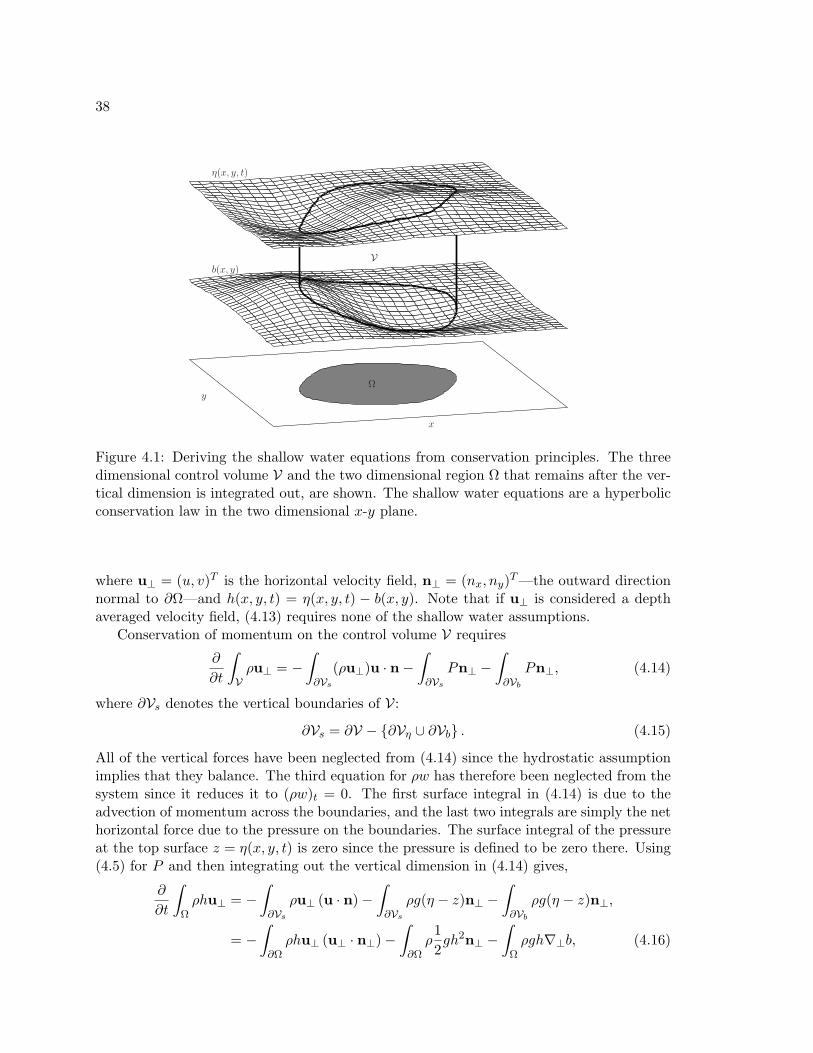
38

x

y

V

η(x, y, t)

b(x, y)

Ω

Figure 4.1: Deriving the shallow water equations from conservation principles. The threedimensional control volume V and the two dimensional region Ω that remains after the ver-tical dimension is integrated out, are shown. The shallow water equations are a hyperbolicconservation law in the two dimensional x-y plane.

where u⊥ = (u, v)T is the horizontal velocity field, n⊥ = (nx, ny)T—the outward directionnormal to ∂Ω—and h(x, y, t) = η(x, y, t) − b(x, y). Note that if u⊥ is considered a depthaveraged velocity field, (4.13) requires none of the shallow water assumptions.

Conservation of momentum on the control volume V requires

∂

∂t

∫Vρu⊥ = −

∫∂Vs

(ρu⊥)u · n−∫∂Vs

Pn⊥ −∫∂Vb

Pn⊥, (4.14)

where ∂Vs denotes the vertical boundaries of V:

∂Vs = ∂V − ∂Vη ∪ ∂Vb . (4.15)

All of the vertical forces have been neglected from (4.14) since the hydrostatic assumptionimplies that they balance. The third equation for ρw has therefore been neglected from thesystem since it reduces it to (ρw)t = 0. The first surface integral in (4.14) is due to theadvection of momentum across the boundaries, and the last two integrals are simply the nethorizontal force due to the pressure on the boundaries. The surface integral of the pressureat the top surface z = η(x, y, t) is zero since the pressure is defined to be zero there. Using(4.5) for P and then integrating out the vertical dimension in (4.14) gives,

∂

∂t

∫Ωρhu⊥ = −

∫∂Vs

ρu⊥ (u · n)−∫∂Vs

ρg(η − z)n⊥ −∫∂Vb

ρg(η − z)n⊥,

= −∫∂Ωρhu⊥ (u⊥ · n⊥)−

∫∂Ωρ12gh2n⊥ −

∫Ωρgh∇⊥b, (4.16)

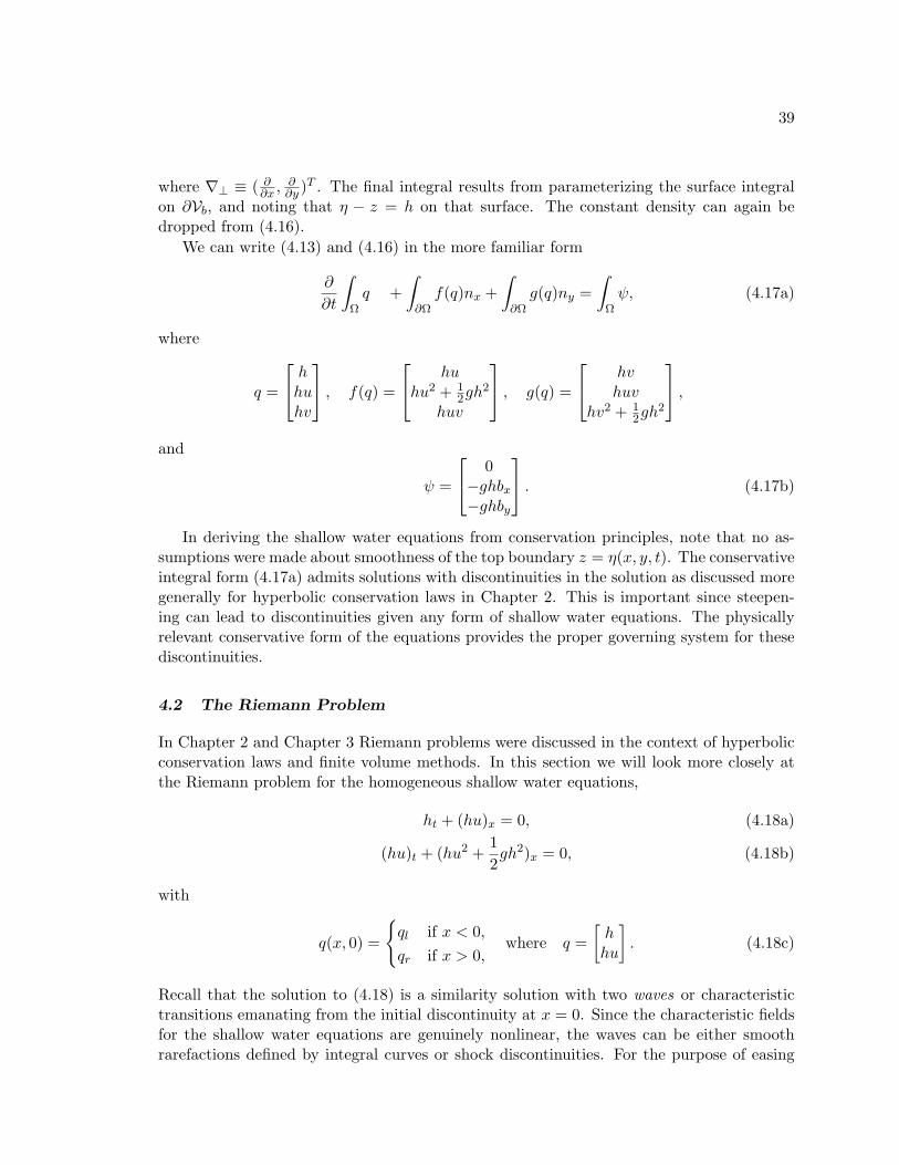
39

where ∇⊥ ≡ ( ∂∂x ,∂∂y )

T . The final integral results from parameterizing the surface integralon ∂Vb, and noting that η − z = h on that surface. The constant density can again bedropped from (4.16).

We can write (4.13) and (4.16) in the more familiar form

∂

∂t

∫Ωq +

∫∂Ωf(q)nx +

∫∂Ωg(q)ny =

∫Ωψ, (4.17a)

where

q =

hhuhv

, f(q) =

huhu2 + 1

2gh2

huv

, g(q) =

hvhuv

hv2 + 12gh

2

,and

ψ =

0−ghbx−ghby

. (4.17b)

In deriving the shallow water equations from conservation principles, note that no as-sumptions were made about smoothness of the top boundary z = η(x, y, t). The conservativeintegral form (4.17a) admits solutions with discontinuities in the solution as discussed moregenerally for hyperbolic conservation laws in Chapter 2. This is important since steepen-ing can lead to discontinuities given any form of shallow water equations. The physicallyrelevant conservative form of the equations provides the proper governing system for thesediscontinuities.

4.2 The Riemann Problem

In Chapter 2 and Chapter 3 Riemann problems were discussed in the context of hyperbolicconservation laws and finite volume methods. In this section we will look more closely atthe Riemann problem for the homogeneous shallow water equations,

ht + (hu)x = 0, (4.18a)

(hu)t + (hu2 +12gh2)x = 0, (4.18b)

with

q(x, 0) =

ql if x < 0,qr if x > 0,

where q =[hhu

]. (4.18c)

Recall that the solution to (4.18) is a similarity solution with two waves or characteristictransitions emanating from the initial discontinuity at x = 0. Since the characteristic fieldsfor the shallow water equations are genuinely nonlinear, the waves can be either smoothrarefactions defined by integral curves or shock discontinuities. For the purpose of easing

40

discussion in this section, zero-strength transitions (or lack of a wave in a family) will beconsidered a rarefaction. For the shallow water equations the Riemann invariants

w1(q) ≡ u+ 2√gh, (4.19a)

w2(q) ≡ u− 2√gh, (4.19b)

hold through an integral curve of the first and second characteristic fields respectively.Discontinuities must obey the Rankine-Hugoniot jump conditions (2.7), which take theform

s

[[hhu

]]=[[

huhu2 + 1

2gh2

]], (4.20)

where [[·]] indicates the difference across the jump discontinuity and s is the propagationspeed of the discontinuity. Recall that the Rankine-Hugoniot conditions can be used toderive the Hugoniot loci, or curves in phase space that can connect two states through ashock. For the shallow water equations, states q∗ that can be connected to ql through a1-shock satisfy

u∗ + h∗

√g

2

(1h∗

+1hl

)= ul + hl

√g

2

(1h∗

+1hl

), (4.21a)

and states q∗ that can be connected to qr through a 2-shock satisfy

u∗ − h∗

√g

2

(1h∗

+1hr

)= ur − hr

√g

2

(1h∗

+1hr

). (4.21b)

Discontinuities must also obey entropy conditions, such as the Lax entropy condition—Definition 2.3— which applies to strictly hyperbolic genuinely nonlinear systems such asthe shallow water equations. For the shallow water equations, simple admissability criteriacan be derived from the Lax entropy condition.

Theorem 4.1. A solution to (4.18) is the correct entropy satisfying solution if and only ifit has the following properties:

(i). A 1-shock connects ql to q∗ if and only if h∗ > hl.

(ii). A 2-shock connects qr to q∗ if and only if h∗ > hr.

(iii). Otherwise rarefactions defined by smooth integral curves of the first or secondcharacteristic field connect q∗ to ql or qr respectively.

Proof. This is a simple consequence of the Lax entropy condition with (4.19) and (4.21).Since the homogeneous shallow water equations are strictly hyperbolic and genuinely nonlin-ear, q∗ is connected to ql by either a 1-shock or a rarefaction in the first characteristic field,and q∗ is connected to qr by either a 2-shock or a rarefaction in the second characteristicfield. It will therefore suffice to prove the contrapositive to (i) and (ii).

41

(⇒) Suppose that a 2-wave connecting qr to q∗ is a rarefaction. By (4.19) and the Laxentropy condition,

0 ≤ λ2(qr)− λ2(q∗)

= ur+√ghr −

(u∗+

√gh∗)

= w2(qr) + 3√ghr −

(w2(q∗) + 3

√gh∗)

= 3(√ghr −

√gh∗), (4.22)

implying h∗ ≤ hr.

(⇐) Conversely, suppose that h∗ ≤ hr. If a 2-shock connects q∗ to qr, then the Lax entropycondition implies: u∗ +

√gh∗ > ur +

√ghr,

⇒ u∗ − ur >√ghr −

√gh∗,

≥ 0 by supposition. (4.23)

Additionally, the two states must lie on the Hugoniot loci for a 2-shock, implying that

u∗ − h∗

√g

2

(1h∗

+1hr

)= ur − hr

√g

2

(1h∗

+1hr

), (4.24)

⇒ u∗ − ur = (h∗ − hr)

√g

2

(1h∗

+1hr

)≤ 0 by supposition. (4.25)

However, (4.23) and (4.25) are contradictory since they imply 0 ≥ u∗ − ur > 0.Therefore, if h∗ ≤ hr, then a rarefaction not a 2-shock must connect qr to q∗. Anentirely analogous proof can be used for 1-waves.

Theorem 4.1 allows us to uniquely determine the middle solution q∗ by using (4.19) and(4.21) such that the properties (i)-(iii) are satisfied. If we define the function

ϕ1(h;hl) =

2(√gh−

√ghl)

if h ≤ hl,

(h− hl)√

g2

(1h + 1

hl

)if h > hl,

(4.26)

then we haveu(h) = ul − ϕ1(h;hl), (4.27)

for u and h through any 1-wave connected to ul. Similarly, if we define the function

ϕ2(h;hr) =

2(√gh−

√ghr)

if h ≤ hr,

(h− hr)√

g2

(1h + 1

hr

)if h > hr,

(4.28)

42

then through any 2-wave we have

u(h) = ur + ϕ2(h;hr). (4.29)

The middle state must occur in phase space where the curves defined by (4.27) and (4.29)intersect. If we subtract the right hand side of (4.27) from (4.29) we have

f(h) = ϕ1(h;hl) + ϕ2(h;hr) + ∆u, h > 0, (4.30)

where ∆u ≡ ur − ul. A root of f(h) determines an intersection in phase space,

f(h∗) = ϕ1(h∗;hl) + ϕ2(h∗;hr) + ∆u = 0, (4.31)

and hence corresponds to a middle state depth h∗. If a root h∗ is found to f(h), then u∗

can be found by evaluating either (4.27) or (4.29).Clearly f(h) is nonlinear, however it has several nice properties in terms of root finding.

These are stated as a theorem for clarity.

Theorem 4.2. The function f(h) defined by (4.30) has the following properties:

(i). It is a monotonically increasing function of h.

(ii). It is continuous and has continuous derivatives, even at h = hl and h = hr.

(iii). It is convex: f ′′(h) < 0.

Theorem 4.2 can be demonstrated through straightforward analysis. See Toro [101] formore details.

By using Theorem 4.1 and Theorem 4.2, a complete characterization of the Riemannstructure can be determined, even without root finding [101]. That is, we can determine ifeach respective wave in the Riemann solution is a shock or rarefaction, simply by evaluatingf(hl) and f(hr). To see this, let

hmin = min(hl, hr), (4.32a)hmax = max(hl, hr). (4.32b)

Now, by Theorem 4.1 and the fact that f(h) is monotonically increasing we have

case 1: f(hmin) ≥ 0 ⇔ two rarefactions,case 2: f(hmax) ≥ 0 > f(hmin) ⇔ one shock, one rarefaction,case 3: f(hmax) < 0 ⇔ two shocks,

. (4.33)

The basis of (4.33) is clear when one considers where the root h∗ must lie relative to hminand hmax. Determining whether case 2 has a 1-shock or 2-shock simply depends on whichis greater hl or hr. Figure 4.2 shows an example of f(h) for each of the three cases. Notethat since f(h) is only defined for h > 0, it is possible that no root will exist. This will bediscussed in detail in the next section, when we consider dry states h = 0.

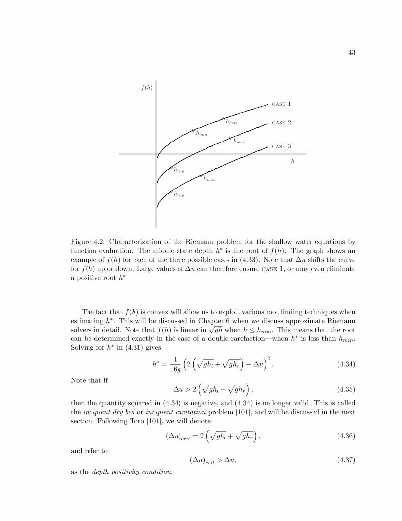
43

h

f(h)

hmin

hmin

hmin

hmax

hmax

hmax

case 1

case 2

case 3

Figure 4.2: Characterization of the Riemann problem for the shallow water equations byfunction evaluation. The middle state depth h∗ is the root of f(h). The graph shows anexample of f(h) for each of the three possible cases in (4.33). Note that ∆u shifts the curvefor f(h) up or down. Large values of ∆u can therefore ensure case 1, or may even eliminatea positive root h∗

The fact that f(h) is convex will allow us to exploit various root finding techniques whenestimating h∗. This will be discussed in Chapter 6 when we discuss approximate Riemannsolvers in detail. Note that f(h) is linear in

√gh when h ≤ hmin. This means that the root

can be determined exactly in the case of a double rarefaction—when h∗ is less than hmin.Solving for h∗ in (4.31) gives

h∗ =1

16g

(2(√

ghl +√ghr

)−∆u

)2. (4.34)

Note that if∆u > 2

(√ghl +

√ghr

), (4.35)

then the quantity squared in (4.34) is negative, and (4.34) is no longer valid. This is calledthe incipient dry bed or incipient cavitation problem [101], and will be discussed in the nextsection. Following Toro [101], we will denote

(∆u)crit = 2(√

ghl +√ghr

), (4.36)

and refer to(∆u)crit > ∆u, (4.37)

as the depth positivity condition.

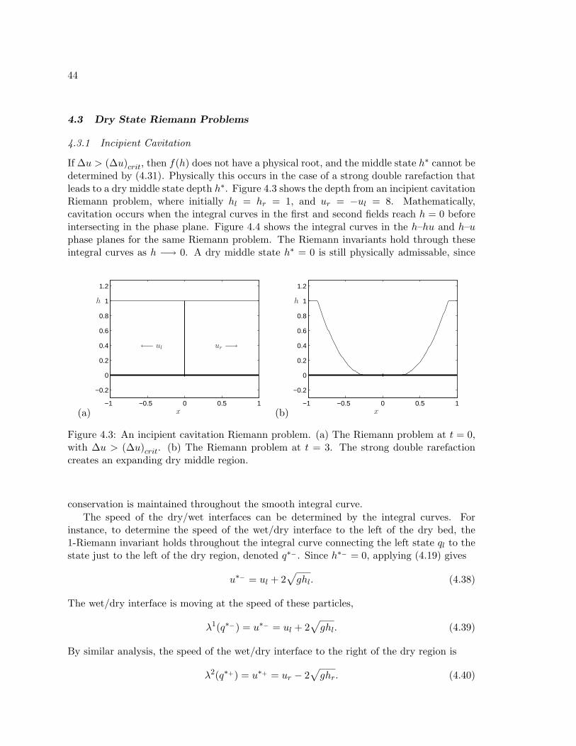
44

4.3 Dry State Riemann Problems

4.3.1 Incipient Cavitation

If ∆u > (∆u)crit, then f(h) does not have a physical root, and the middle state h∗ cannot bedetermined by (4.31). Physically this occurs in the case of a strong double rarefaction thatleads to a dry middle state depth h∗. Figure 4.3 shows the depth from an incipient cavitationRiemann problem, where initially hl = hr = 1, and ur = −ul = 8. Mathematically,cavitation occurs when the integral curves in the first and second fields reach h = 0 beforeintersecting in the phase plane. Figure 4.4 shows the integral curves in the h–hu and h–uphase planes for the same Riemann problem. The Riemann invariants hold through theseintegral curves as h −→ 0. A dry middle state h∗ = 0 is still physically admissable, since

(a)−1 −0.5 0 0.5 1

−0.2

0

0.2

0.4

0.6

0.8

1

1.2

h

x

←− ul ur −→

(b)−1 −0.5 0 0.5 1

−0.2

0

0.2

0.4

0.6

0.8

1

1.2

h

x

Figure 4.3: An incipient cavitation Riemann problem. (a) The Riemann problem at t = 0,with ∆u > (∆u)crit. (b) The Riemann problem at t = 3. The strong double rarefactioncreates an expanding dry middle region.

conservation is maintained throughout the smooth integral curve.The speed of the dry/wet interfaces can be determined by the integral curves. For

instance, to determine the speed of the wet/dry interface to the left of the dry bed, the1-Riemann invariant holds throughout the integral curve connecting the left state ql to thestate just to the left of the dry region, denoted q∗− . Since h∗− = 0, applying (4.19) gives

u∗− = ul + 2√ghl. (4.38)

The wet/dry interface is moving at the speed of these particles,

λ1(q∗−) = u∗− = ul + 2√ghl. (4.39)

By similar analysis, the speed of the wet/dry interface to the right of the dry region is

λ2(q∗+) = u∗+ = ur − 2√ghr. (4.40)

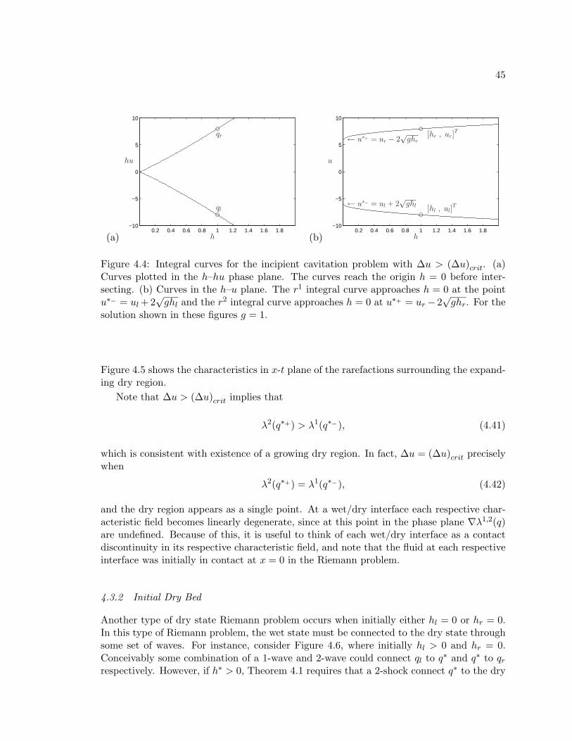
45

(a)0.2 0.4 0.6 0.8 1 1.2 1.4 1.6 1.8

−10

−5

0

5

10

h

hu

qr

ql

(b)0.2 0.4 0.6 0.8 1 1.2 1.4 1.6 1.8

−10

−5

0

5

10

[hl , ul]T

[hr , ur]T

h

u

← u∗+ = ur − 2√

ghr

← u∗− = ul + 2√

ghl

Figure 4.4: Integral curves for the incipient cavitation problem with ∆u > (∆u)crit. (a)Curves plotted in the h–hu phase plane. The curves reach the origin h = 0 before inter-secting. (b) Curves in the h–u plane. The r1 integral curve approaches h = 0 at the pointu∗− = ul +2

√ghl and the r2 integral curve approaches h = 0 at u∗+ = ur− 2

√ghr. For the

solution shown in these figures g = 1.

Figure 4.5 shows the characteristics in x-t plane of the rarefactions surrounding the expand-ing dry region.

Note that ∆u > (∆u)crit implies that

λ2(q∗+) > λ1(q∗−), (4.41)

which is consistent with existence of a growing dry region. In fact, ∆u = (∆u)crit preciselywhen

λ2(q∗+) = λ1(q∗−), (4.42)

and the dry region appears as a single point. At a wet/dry interface each respective char-acteristic field becomes linearly degenerate, since at this point in the phase plane ∇λ1,2(q)are undefined. Because of this, it is useful to think of each wet/dry interface as a contactdiscontinuity in its respective characteristic field, and note that the fluid at each respectiveinterface was initially in contact at x = 0 in the Riemann problem.

4.3.2 Initial Dry Bed

Another type of dry state Riemann problem occurs when initially either hl = 0 or hr = 0.In this type of Riemann problem, the wet state must be connected to the dry state throughsome set of waves. For instance, consider Figure 4.6, where initially hl > 0 and hr = 0.Conceivably some combination of a 1-wave and 2-wave could connect ql to q∗ and q∗ to qrrespectively. However, if h∗ > 0, Theorem 4.1 requires that a 2-shock connect q∗ to the dry

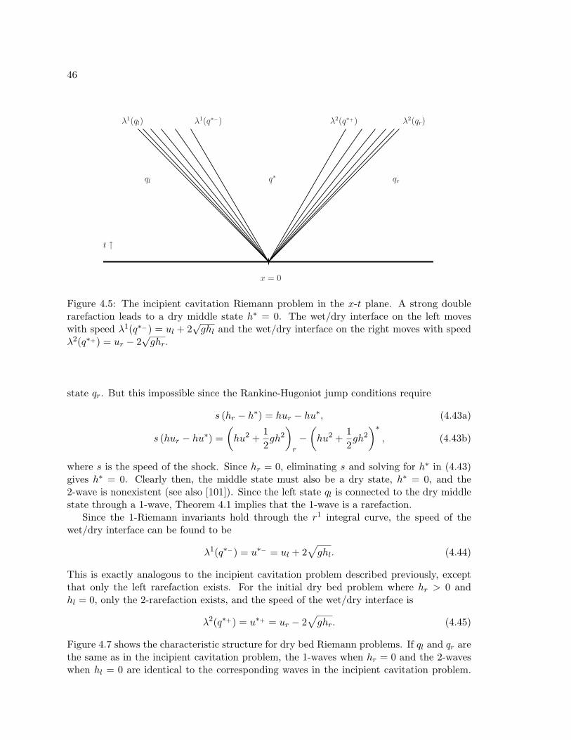
46

x = 0

t ↑

qrql q∗

λ1(ql) λ2(qr)λ1(q∗−) λ2(q∗+)

Figure 4.5: The incipient cavitation Riemann problem in the x-t plane. A strong doublerarefaction leads to a dry middle state h∗ = 0. The wet/dry interface on the left moveswith speed λ1(q∗−) = ul + 2

√ghl and the wet/dry interface on the right moves with speed

λ2(q∗+) = ur − 2√ghr.

state qr. But this impossible since the Rankine-Hugoniot jump conditions require

s (hr − h∗) = hur − hu∗, (4.43a)

s (hur − hu∗) =(hu2 +

12gh2

)r

−(hu2 +

12gh2

)∗, (4.43b)

where s is the speed of the shock. Since hr = 0, eliminating s and solving for h∗ in (4.43)gives h∗ = 0. Clearly then, the middle state must also be a dry state, h∗ = 0, and the2-wave is nonexistent (see also [101]). Since the left state ql is connected to the dry middlestate through a 1-wave, Theorem 4.1 implies that the 1-wave is a rarefaction.

Since the 1-Riemann invariants hold through the r1 integral curve, the speed of thewet/dry interface can be found to be

λ1(q∗−) = u∗− = ul + 2√ghl. (4.44)

This is exactly analogous to the incipient cavitation problem described previously, exceptthat only the left rarefaction exists. For the initial dry bed problem where hr > 0 andhl = 0, only the 2-rarefaction exists, and the speed of the wet/dry interface is

λ2(q∗+) = u∗+ = ur − 2√ghr. (4.45)

Figure 4.7 shows the characteristic structure for dry bed Riemann problems. If ql and qr arethe same as in the incipient cavitation problem, the 1-waves when hr = 0 and the 2-waveswhen hl = 0 are identical to the corresponding waves in the incipient cavitation problem.

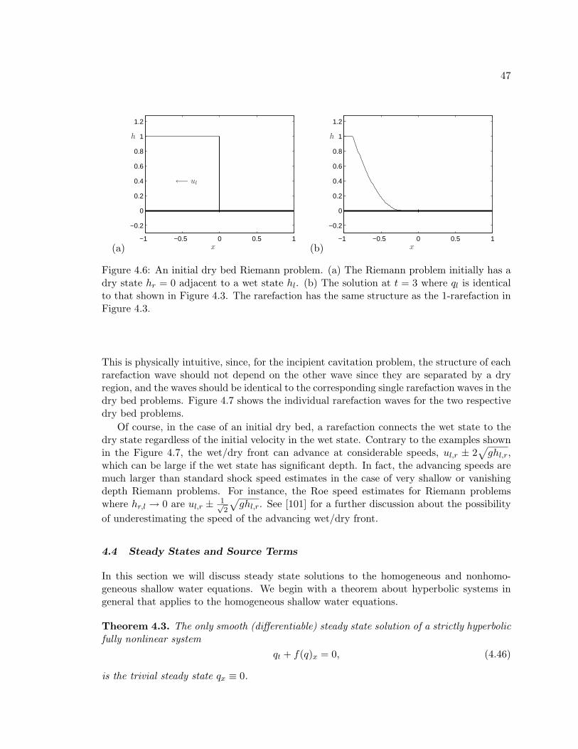
47

(a)−1 −0.5 0 0.5 1

−0.2

0

0.2

0.4

0.6

0.8

1

1.2

h

x

←− ul

(b)−1 −0.5 0 0.5 1

−0.2

0

0.2

0.4

0.6

0.8

1

1.2

h

x

Figure 4.6: An initial dry bed Riemann problem. (a) The Riemann problem initially has adry state hr = 0 adjacent to a wet state hl. (b) The solution at t = 3 where ql is identicalto that shown in Figure 4.3. The rarefaction has the same structure as the 1-rarefaction inFigure 4.3.

This is physically intuitive, since, for the incipient cavitation problem, the structure of eachrarefaction wave should not depend on the other wave since they are separated by a dryregion, and the waves should be identical to the corresponding single rarefaction waves in thedry bed problems. Figure 4.7 shows the individual rarefaction waves for the two respectivedry bed problems.

Of course, in the case of an initial dry bed, a rarefaction connects the wet state to thedry state regardless of the initial velocity in the wet state. Contrary to the examples shownin the Figure 4.7, the wet/dry front can advance at considerable speeds, ul,r ± 2

√ghl,r,

which can be large if the wet state has significant depth. In fact, the advancing speeds aremuch larger than standard shock speed estimates in the case of very shallow or vanishingdepth Riemann problems. For instance, the Roe speed estimates for Riemann problemswhere hr,l → 0 are ul,r ± 1√

2

√ghl,r. See [101] for a further discussion about the possibility

of underestimating the speed of the advancing wet/dry front.

4.4 Steady States and Source Terms

In this section we will discuss steady state solutions to the homogeneous and nonhomo-geneous shallow water equations. We begin with a theorem about hyperbolic systems ingeneral that applies to the homogeneous shallow water equations.

Theorem 4.3. The only smooth (differentiable) steady state solution of a strictly hyperbolicfully nonlinear system

qt + f(q)x = 0, (4.46)

is the trivial steady state qx ≡ 0.

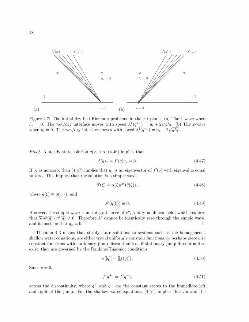
48

(a) x = 0

t ↑

qrql

λ1(ql) λ1(q∗−)

hr = 0

(b) x = 0

t ↑

qrql

λ2(qr)λ2(q∗+)

hl = 0

Figure 4.7: The initial dry bed Riemann problems in the x-t plane. (a) The 1-wave whenhr = 0. The wet/dry interface moves with speed λ1(q∗−) = ul + 2

√ghl. (b) The 2-wave

when hl = 0. The wet/dry interface moves with speed λ2(q∗+) = ur − 2√ghr.

Proof. A steady state solution q(x, ·) to (4.46) implies that

f(q)x = f ′(q)qx = 0. (4.47)

If qx is nonzero, then (4.47) implies that qx is an eigenvector of f ′(q) with eigenvalue equalto zero. This implies that the solution is a simple wave

q′(ξ) = α(ξ)rp (q(ξ)) , (4.48)

where q(ξ) ≡ q(x, ·), and

λp(q(ξ)) ≡ 0. (4.49)

However, the simple wave is an integral curve of rp, a fully nonlinear field, which requiresthat ∇λp(q) · rp(q) 6= 0. Therefore λp cannot be identically zero through the simple wave,and it must be that qx ≡ 0.

Theorem 4.3 means that steady state solutions to systems such as the homogeneousshallow water equations, are either trivial uniformly constant functions, or perhaps piecewiseconstant functions with stationary jump discontinuities. If stationary jump discontinuitiesexist, they are governed by the Rankine-Hugoniot conditions

s [[q]] = [[f(q)]] . (4.50)

Since s = 0,

f(q+) = f(q−), (4.51)

across the discontinuity, where q+ and q− are the constant states to the immediate leftand right of the jump. For the shallow water equations, (4.51) implies that hu and the

49

momentum flux (hu2 + 12gh

2) do not vary across a stationary discontinuity. Since themomentum flux is a nonlinear function of h and hu, in general it is possible to have astationary jump in h. This jump must also satisfy entropy conditions.

4.4.1 Source Terms

More complex steady states exist when source terms are included,

qt + f(q)x + ψ, (4.52)

since the balance of ψ and the flux gradient f(q)x imply that qt = 0. Note that for theshallow water equations over variable bathymetry,

ht + (hu)x = 0, (4.53a)

hut +(hu2 +

12gh2

)x

= −ghbx, (4.53b)

this occurs when

(hu)x = 0, (4.54a)(hu2 +

12gh2

)x

= −ghbx. (4.54b)

As with the homogeneous shallow water equations, (4.54a) implies that hu is always constantfor steady states, otherwise mass would accumulate in certain regions. However, (4.54b)implies that the momentum flux must balance the source term for steady states. Since themomentum flux is only a function of h and hu, h must vary through a steady state wherebx 6= 0. If we differentiate the momentum flux in (4.54b), while holding hu constant, wehave (

−u2 + gh)hx = −ghbx. (4.55)

Since the eigenvalues for the shallow water equations satisfy −λ1λ2 = −u2 + gh, it shouldbe noted that a smooth steady state over sloping bathymetry cannot have a sonic point.Therefore, for regions with monotonically varying bathymetry, steady-state flow is eitherentirely subsonic or entirely supersonic. If the flow is subsonic

(−u2 + gh > 0

), hx and bx

are opposite in sign, with the opposite being true if the flow is supersonic. The transitioncan only occur at an extremum of the bathymetry where bx = 0.

In section Section 2.3, it was mentioned that the Rankine-Hugoniot conditions are un-changed in the presence of a bounded source term. Therefore, for a steady state in the formof a stationary jump discontinuity, (4.51) still holds as long as bx is defined continuously, orif bx is bounded in a neighborhood of the jump. However, for developing numerical methods,it is useful to consider b(x) as a piecewise constant function, and allow bx to be a sum ofgeneralized distributions equal to a delta function at each jump discontinuity,

bx ≡∑xj∈X

(b(x+

j )− b(x−j ))δ(x− xj), (4.56)

50

where X contains the locations of the jump discontinuities in b(x), and δ(x) is the deltafunction defined by ∫

δ(x)f(x) = f(0). (4.57)

The source term in the shallow water equations, −ghbx, is not necessarily well defined by(4.56), even in the sense of a distribution, since it involves h, which is possibly (in factnecessarily for steady states) discontinuous at xj ∈ X . This creates a problem for thetheory of distributions involving overlapping discontinuities. See also [26], and for somediscussion of overlapping discontinuities and distribution theory, see [18]. However, wesuspend uncertainty temporarily and assume that the source term is a sum of point sourcesat the locations xj . We write the source term as a sum of distributions

−ghbx = ψ =∑xj∈X

Ψjδ(x− xj), (4.58)

which integrated across a jump discontinuity gives∫ x+j

x−j

ψ dx = Ψj . (4.59)

If we then apply the integral conservation law to a neighborhood around the single discon-tinuity at xj , we have

(hu)+ = (hu)−, (4.60a)(hu2 +

12gh2

)+

−(hu2 +

12gh2

)−= Ψj , (4.60b)

where for notational ease the superscripts (·)+, (·)− denote evaluation at x+,−j . The condi-

tions (4.60) are similar to the Rankine-Hugoniot conditions for a stationary discontinuityover continuous bathymetry (4.51), except now the infinite source term contributes a righthand side to (4.60b). This follows physical intuition, since if the jump in momentum flux didnot balance the point source of momentum, the solution would quickly become unboundedin the neighborhood of the discontinuity. As with (4.51), the momentum hu is constant andso a jump in momentum flux implies that only h varies across the stationary discontinuity.This is what causes the difficulty in defining the source term by (4.56) and (4.57), since∫

−gh(x)(b(x+

j )− b(x−j ))δ(x− xj), (4.61)

is not clearly defined when h is discontinuous at xj . Note however that (4.60) defines Ψj interms of the left and right states, q−,+, on either side of the discontinuity.

It is informative to consider the steady state problem with zero velocity, where η ≡h + b ≡ 0 everywhere. Based on physical intuition, this is obviously the correct limitingsteady state solution even when b(x) is a piecewise constant function. Evaluating (4.60)

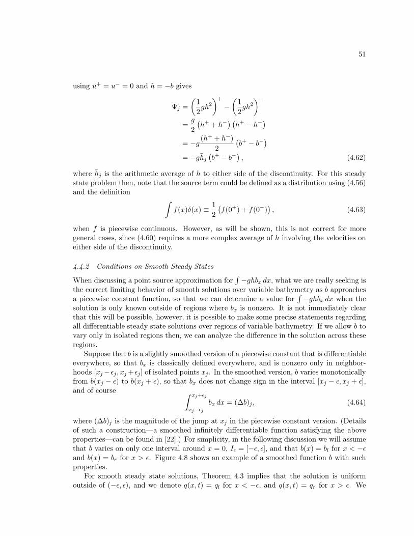
51

using u+ = u− = 0 and h = −b gives

Ψj =(

12gh2

)+

−(

12gh2

)−=g

2(h+ + h−

) (h+ − h−

)= −g (h+ + h−)

2(b+ − b−

)= −ghj

(b+ − b−

), (4.62)

where hj is the arithmetic average of h to either side of the discontinuity. For this steadystate problem then, note that the source term could be defined as a distribution using (4.56)and the definition ∫

f(x)δ(x) ≡ 12(f(0+) + f(0−)

), (4.63)

when f is piecewise continuous. However, as will be shown, this is not correct for moregeneral cases, since (4.60) requires a more complex average of h involving the velocities oneither side of the discontinuity.

4.4.2 Conditions on Smooth Steady States

When discussing a point source approximation for∫−ghbx dx, what we are really seeking is

the correct limiting behavior of smooth solutions over variable bathymetry as b approachesa piecewise constant function, so that we can determine a value for

∫−ghbx dx when the

solution is only known outside of regions where bx is nonzero. It is not immediately clearthat this will be possible, however, it is possible to make some precise statements regardingall differentiable steady state solutions over regions of variable bathymetry. If we allow b tovary only in isolated regions then, we can analyze the difference in the solution across theseregions.

Suppose that b is a slightly smoothed version of a piecewise constant that is differentiableeverywhere, so that bx is classically defined everywhere, and is nonzero only in neighbor-hoods [xj−εj , xj+εj ] of isolated points xj . In the smoothed version, b varies monotonicallyfrom b(xj − ε) to b(xj + ε), so that bx does not change sign in the interval [xj − ε, xj + ε],and of course ∫ xj+εj

xj−εjbx dx = (∆b)j , (4.64)

where (∆b)j is the magnitude of the jump at xj in the piecewise constant version. (Detailsof such a construction—a smoothed infinitely differentiable function satisfying the aboveproperties—can be found in [22].) For simplicity, in the following discussion we will assumethat b varies on only one interval around x = 0, Iε = [−ε, ε], and that b(x) = bl for x < −εand b(x) = br for x > ε. Figure 4.8 shows an example of a smoothed function b with suchproperties.

For smooth steady state solutions, Theorem 4.3 implies that the solution is uniformoutside of (−ε, ε), and we denote q(x, t) = ql for x < −ε, and q(x, t) = qr for x > ε. We

52

0−ǫ ǫ

bl

br

Figure 4.8: A smoothed version of piecewise constant bathymetry. The function shown isC∞(lR), and bx has compact support on [−ε, ε]. Additionally the function is symmetric,b(0) = (br + bl)/2.

can derive some conditions relating the left and right states, ql and qr, and the “jump” inbathymetry

∆b = (br − bl). (4.65)

(In many of the equations that follow, the operator ∆ will refer to differencing the quan-tities from the right to the left ∆(·) = (·)r − (·)l, where the subscripts refer to evaluatingthe quantities in the constant region to the right and left respectively.) First, (hu)x = 0everywhere, so

∆hu = hur − hul = 0. (4.66)

Using this fact, we can relate the jump in the momentum flux,

∆(hu2 +

12gh2

)=(hu2 +

12gh2

)r

−(hu2 +

12gh2

)l

, (4.67)

to the difference or jump in the depth

∆h = (hr − hl) . (4.68)

53

We rearrange (4.60b),

∆(hu2 +

12gh2

)=(

(hu)2

hr− (hu)2

hl

)+g

2(hr + hl) (hr − hl)

=(|(hu)r(hu)l|

hr− |(hu)l(hu)r|

hl

)+g

2(hr + hl) (hr − hl)

= (hl|urul| − hr|+ ulur|) +g

2(hr + hl) (hr − hl)

= ∆h(−|urul|+

g

2(hr + hl)

), (4.69)

where h ≥ 0 and hur = hul together imply that urul = |urul|. If we denote the averages

h = 12(hr + hl), (4.70a)

u2 = |urul|, (4.70b)

we can rewrite (4.69) as

∆φ =(−u2 + gh

)∆h, (4.71)

where φ is the momentum flux φ = (hu2 + 12gh

2). This notation for the momentum fluxwill be used frequently in the remaining chapters. The ratio implied by (4.71) is essentiallya discrete version of the partial derivative of the momentum flux φ with respect to h, whileholding hu constant, (

∂φ

∂h

)hu

= −u2 + gh, (4.72)

and requires the special averages (4.70) of the left and right states when ∆q is not infinites-imal. Equation (4.71) may also be viewed as an exact first order Taylor expansion, wherethe partial derivative is evaluated at the intermediate state defined by (4.70).

We can also relate ∆h to ∆b for smooth solutions. Consider (4.55), which is exactlytrue for differentiable steady state solutions. Dividing by h gives(

−(hu)2

h3+ g

)hx = −gbx. (4.73)

By noting that (hu)x ≡ 0 for steady states, it can be seen that (4.73) is equivalent to(12

(hu)2

h2+ gh+ gb

)x

= 0, (4.74)

which implies that(

12u

2 + gh+ gb)

is a constant for a differentiable steady state. So it mustbe true that (

12u2 + gh+ gb

)r

=(

12u2 + gh+ gb

)l

. (4.75)

54

Multiplying (4.75) by h = 12(hr + hl) and rearranging gives,

−gh∆b− gh∆h =(hr + hl

2

)(u2r − u2

l

2

)=(

12

)2 (hru

2r + hlu

2r − hru

2l − hlu

2l

)=(

12

)2 ((2hru2

r − hru2r

)+ hlu

2r − hru

2l −

(2hlu2

l − hlu2l

))=(

12

)2 ((2hlulur − hru

2r

)+ hlu

2r − hru

2l −

(2hrurul − hlu

2l

))=(

12

)2 ((hlu

2l + 2hlulur + hlu

2r

)−(hru

2l + 2hrulur + hru

2r

))=(

12

)2 (hl (ur + ul)

2 − hr (ur + ul)2)

= −(ur + ul

2

)2

∆h, (4.76)

where the fourth equality makes use of hlul = hrur. Equation (4.76) implies the relationship(−u2 + gh

)∆h = −gh∆b, (4.77)

where u is the arithmetic average 12 (ul + ur). Note that this is a discrete representation

of (4.55), or an exact first order Taylor expansion for steady states, using the arithmeticaverages of h and u.

Since (4.71) relates ∆h to ∆φ, equation (4.77) allows us to relate ∆φ to ∆b,

∆φ = −gh∆b

(−u2 + gh

−u2 + gh

). (4.78)

By applying conservation,

∆φ =∫Iε

−ghbx dx, (4.79)

the right hand side of equation (4.78) provides the correct formulation of the source termfor all smooth steady states across an interval of varying bathymetry. For these solutions,it must be true that ∫

Iε

−ghbx dx = −S+−gh∆b. (4.80)

where,

S+− =

(−u2 + gh

−u2 + gh

). (4.81)

The ratio S+− is a nondimensional quantity that provides the correct source term inte-

gral when multiplied by −gh∆b, for smooth steady states across any region of varying

55

bathymetry br− bl = ∆b. (The notation is meant to resemble an integral, since the product−S+

−gh∆b is equal to the value of the integral −∫Iεghbx dx.) Note that for smooth solu-

tions, if ql → qr, then S+− → 1. It might at first seem curious that S+

− could be negative,even if bx does not change sign, or worse, the denominator might vanish. However, recallthat we have found that steady flow cannot have a sonic point when b varies monotonicallyby (4.55), therefore, such flows must be entirely subsonic or supersonic. By requiring theFroude number, |u/gh|, to be either strictly less than or more than one for all x, it is easyto demonstrate that the ratio (4.81) is always positive for these flows. In fact, since

u2 ≥ urul, ∀ul, ur ∈ lR, (4.82)

with equality only when ur = ul, it follows that S+− is less than unity for supersonic flow, and

greater than or equal to unity for subsonic flow, with equality only for stationary flow withzero velocity—following from the fact that ul = ur implies that hl = hr unless ul = ur = 0.(Equality of depth across variable bathymetry is a contradiction because of (4.55).) Foru ≡ 0, the ratio S+

− = 1 produces the desired result (4.62) for the source term.Equation (4.55) relating hx and bx for smooth steady flows, allows further characteriza-

tion of −gh∆bS+− . Since the flow in question has no sonic points, hx cannot change sign,

and h must vary monotonically from hl to hr across the interval where b varies. Therefore,the integral for the source term can be bounded,

|S+−gh∆b| = |

∫Iε

ghbx dx|

≤ gmax(hl, hr)|∫Iε

bx dx|

= gmax(hl, hr)|∆b|, (4.83)

and similarly|S+−gh∆b| ≥ gmin(hl, hr)|∆b|. (4.84)

We can therefore statemin(hl, hr) ≤ S+

− h ≤ max(hl, hr), (4.85)

for smooth steady states.

4.4.3 Steady State Data

In this final section, the properties of smooth steady state solutions over monotonicallyvarying bathymetry will be summarized by presenting them in a simple unified manner.A discontinuous steady state will be briefly discussed as well. We will consider only acontinuously differentiable bathymetry function b(x), such as that discussed in the previoussection and depicted in Figure 4.8, where b(x) = bl to the left of an interval Iε and b(x) = brto the right of the interval, and b(x) varies monotonically in the interval. It has beenshown that this implies that the steady state solution must also be uniform to the left andright of the interval, and h varies monotonically in the interval. Concisely summarizing theproperties that must be satisfied by the left and right states is the goal of this section.

56

It will be convenient to define some of the averages discussed above, as operators actingon two states ql and qr. First, we will define the operators

λ1λ2(ql, qr) = −

(−(ul + ur

2

)2

+ g

(hr + hl

2

)), (4.86)

and

λ1λ2(ql, qr) = −(−ulur + g

(hr + hl

2

)). (4.87)

The negative signs are introduced in the right hand sides of (4.86) and (4.87), so that theoperators represent an approximation to the product of the eigenvalues of the shallow waterequations λ1(q)λ2(q) = (u2 − gh). We also introduce the operator

S+− (ql, qr) = −g

2(hr + hl)

λ1λ2(ql, qr)

λ1λ2(ql, qr), (4.88)

which is equivalent to (4.81), except that we have absorbed the −gh. The operator thensatisfies the following property,

S+− (ql, qr)∆b = −

∫ghbx dx, (4.89)

if it is evaluated by left and right states that correspond to a smooth steady state. We nowstate some results as a theorem, for emphasis and for convenient reference in the followingchapters.

Theorem 4.4. Given a monotonically varying smooth bathymetry function such as thatdescribed above, the following property must be satisfied for all smooth steady state data, qland qr,

∆

hhuφb

= ∆b

S+−(ql,qr)

−gλ1λ2(ql,qr)

0S+− (ql, qr)

1

, (4.90)

where ∆ implies subtracting the quantities evaluated with data ql from those evaluated withqr.

Proof. The theorem follows from simply considering the ratios developed in the previoussection, and the fact that (hu)x ≡ 0.

It is interesting to consider what happens if we allow a discontinuity in the steady stateover monotonically varying smooth bathymetry. For instance, suppose that the solutionto the left of the interval Iε, q(x < −ε, t) = ql, is joined to solution to the right of Iε,q(x > ε, t) = qr, through a smooth transition on either side of a discontinuity at x = 0,with q(0−, t) = q− and q(0+, t) = q+. Recall that when b is continuously differentiable,a discontinuous solution is still governed by the Rankine-Hugoniot (4.50) conditions for a

57

shock. For a steady state, the shock is stationary, and the fluxes must be constant acrossthe discontinuity (4.51). So we have, assuming that b(x) is continuously differentiable,

∆

hhuφb

= ∆h

1000

, (4.91)

where ∆ is the difference just across the discontinuity.It should be noted that the relation (4.71) is valid across the discontinuity, and because

the flux is constant it must be that λ1λ2(q−, q+) = 0. In fact, λ1λ2(q−, q+) = 0 for anystationary discontinuity where q− and q+ are the states to the left and right of the discon-tinuity, which follows from relating (4.55) to the Rankine-Hugoniot conditions governing astationary shock.)

Conservation applied around the interval Iε still requires that

f(qr)− f(ql) = −∫Iε

ghbx dx. (4.92)

Since the right hand side of (4.92) is nonzero, f(q−) = f(q+), and hu does not vary, hmust vary through the smooth regions and the total change (hr − hl) must be nonzero.Therefore, over a region of monotonically varying bathymetry, ql cannot be connected toqr with a single stationary shock. Since (4.71) still holds using ql and qr, it cannot be thatλ1λ2(ql, qr) = 0. Therefore, the total jump ∆h = (hr−hl) is well defined by (4.71). Since astationary shock implies that the flow is supersonic to one side of the shock and subsonic tothe other, it is not clear if a general statement can be made about the sign of λ1λ2(ql, qr),however, it is apparent that hx is positive to one side of the discontinuity and negative tothe other because of (4.55). We can summarize these properties most easily by first definingthe augmented state variable

q(q, b) =

hhuφb

. (4.93)

For all steady state data, ql and qr, to the left and right of a region of monotonically smoothlyvarying bathymetry, q(qr, br) and q(ql, bl) can be connected by a linear combination of thetwo vectors

1000

, and

−Rghbx

−λ1λ2(ql,qr)

0−∫ghbx

br − bl

, (4.94)

where λ1λ2(ql, qr) is guaranteed to be nonzero. Additionally, when the solution is continu-ously differentiable

−∫ghbx dx = S+

− (ql, qr)∆b. (4.95)

58

Chapter 5

NUMERICAL TSUNAMI MODELING

Physical aspects of tsunamis will be addressed in this chapter, and the resulting chal-lenges that must be confronted by numerical modelers will be described. We begin by firstconsidering the generation of tsunamis and governing approximations for tsunami flows.

5.1 Tsunami Generation and Governing Assumptions

Tsunamis can be generated by a variety of geophysical disturbances—most commonly earth-quakes, landslides, or some combination of the two. Because of the diverse physical natureof these disturbances, tsunamis can vary greatly in their size and extent, however, all canbe destructive and deadly. Typically, landslide generated tsunamis are more localized, yet,large submarine landslides can generate oceanic tsunamis impacting an entire region. Forinstance, the Papua New Guinea Tsunami of 1998, which killed over 2000 people, is believedto have been caused by a submarine landslide following an earthquake. A more localizedtsunami due to an underwater landslide occurred in 1994 at Skagway Harbor, Alaska, wherea cruise ship wharf undergoing construction collapsed [57].

The most notable tsunamis are the large earthquake-generated global-scale tsunamisthat can affect coastlines around an entire oceanic region, such as the recent Indian OceanTsunami. The generating mechanism for these tsunamis is believed to be the verticaluplift of the water column due to the displacement of the ocean floor, not the seismicwaves or the horizontal momentum of the fault plane. It is therefore the geometry of afault mechanism that determines whether a seismic event is tsunamigenic. If the verticaldisplacement of the water column is the principle tsunamigenic mechanism, then tsunamiwaves begin as long waves—waves governed by the shallow water equations. This is becausethe horizontal length scales of most fault displacements are far greater than the depth of theocean, and additionally, vertical displacement of the ocean floor creates initial conditionsthat are invariant in the vertical direction—the entire water column is lifted and remainshydrostatic. Recently, it has been argued by some (e.g. Rivera [81]) that the horizontalmotion of the fault plane is a significant ingredient in tsunami initiation by impartingmomentum to the water column. If this is true, then vertically varying horizontal fluidmomentum would play a significant role in tsunamigenesis, and these effects would not begoverned by the shallow water approximation. However, it is more traditionally believedthat such motion is not transferred to the long-wave gravity waves of tsunami propagation.See [92] for a discussion of tsunamigenic sea-floor deformations.

There is growing evidence that dispersive effects may be more important in tsunamipropagation than previously thought. See, for instance, [34],[46] and [58] for some empir-ical arguments. The largest terms neglected in the shallow water equations are dispersiveterms, which might be desirable for more accurate modeling of tsunamis in certain cases.

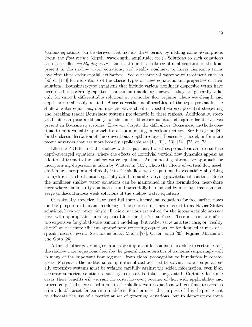
59

Various equations can be derived that include these terms, by making some assumptionsabout the flow regime (depth, wavelength, amplitude, etc.). Solutions to such equationsare often called weakly-dispersive, and exist due to a balance of nonlinearities, of the kindpresent in the shallow water equations, and weakly nonlinear to linear dispersive termsinvolving third-order spatial derivatives. See a theoretical water-wave treatment such as[50] or [103] for derivations of the classic types of these equations and properties of theirsolutions. Boussinesq-type equations that include various nonlinear dispersive terms havebeen used as governing equations for tsunami modeling, however, they are generally validonly for smooth differentiable solutions in particular flow regimes where wavelength anddepth are predictably related. Since advection nonlinearities, of the type present in theshallow water equations, dominate as waves shoal in coastal waters, potential steepeningand breaking render Boussinesq systems problematic in these regions. Additionally, steepgradients can pose a difficulty for the finite difference solution of high-order derivativespresent in Boussinesq systems. However, despite the difficulties, Boussinesq methods con-tinue to be a valuable approach for ocean modeling in certain regimes. See Peregrine [80]for the classic derivation of the conventional depth averaged Boussinesq model, or for morerecent advances that are more broadly applicable see [1], [31], [53], [74], [75] or [78].

Like the PDE form of the shallow water equations, Boussinesq equations are free-surfacedepth-averaged equations, where the effects of nontrivial vertical flow dynamics appear asadditional terms to the shallow water equations. An interesting alternative approach forincorporating dispersion is taken by Walters in [102], where the effects of vertical flow accel-eration are incorporated directly into the shallow water equations by essentially absorbingnonhydrostatic effects into a spatially and temporally varying gravitational constant. Sincethe nonlinear shallow water equations can be maintained in this formulation, near-shoreflows where nonlinearity dominates could potentially be modeled by methods that can con-verge to discontinuous weak solutions of the shallow water equations.

Occasionally, modelers have used full three dimensional equations for free surface flowsfor the purpose of tsunami modeling. These are sometimes referred to as Navier-Stokessolutions, however, often simple elliptic equations are solved for the incompressible internalflow, with appropriate boundary conditions for the free surface. These methods are oftentoo expensive for global-scale tsunami modeling, but rather serve as a test case, or “realitycheck” on the more efficient approximate governing equations, or for detailed studies of aspecific area or event. See, for instance, Mader [73], Gisler et al [30], Fujima, Masamuraand Goto [25].

Although other governing equations are important for tsunami modeling in certain cases,the shallow water equations describe the general characteristics of tsunamis surprisingly wellin many of the important flow regimes—from global propagation to inundation in coastalareas. Moreover, the additional computational cost accrued by solving more computation-ally expensive systems must be weighed carefully against the added information, even if anaccurate numerical solution to such systems can be taken for granted. Certainly for somecases, these benefits will warrant the costs, however, because of their wide applicability andproven empirical success, solutions to the shallow water equations will continue to serve asan invaluable asset for tsunami modelers. Furthermore, the purpose of this chapter is notto advocate the use of a particular set of governing equations, but to demonstrate some

60

properties that are required of numerical methods used for solving the shallow water equa-tions for tsunami modeling. Other governing systems present their own set of numericalchallenges—a modern approach for solving Boussinesq systems can be found in [86], andthe use of Navier-Stokes equations for tsunami modeling is covered in [73].

5.2 The Diverse Regimes of Tsunami Flow

In this section, we will take the governing equations—the shallow water equations—forgranted, and discuss the diversity of flow regimes exhibited by solutions to these equations inthe context of tsunamis. These diverse flow regimes demand diverse properties of numericalmethods, and it must be emphasized that not all consistent numerical methods for theshallow water equations will produce accurate solutions for flows in these regimes.

In the deep ocean, the wavelength of a typical tsunami wave is very long—on the order ofseveral hundred kilometers—while the depth of the ocean is typically only a few kilometers.If we define the parameter δ to be the ratio of depth divided by wavelength, the shallowwater approximation comes from assuming that δ is small resulting in the implication thatvertical variation in the flow is negligible. These properties are what allow tsunami energy topropagate thousands of miles away from a source before being dissipated. (This is anotherargument for the shallow water approximation—large vertical variations in the water columnare more quickly dissipated, and not transmitted in the transoceanic waves. Certainly onthe sea floor near a rupturing fault, complex, even turbulent flows must exist, but thisenergy is quickly dissipated, and the potential energy associated with the vertical uplift iswhat is carried away with the tsunami.) Contrasted to the wavelength, the amplitude oftsunami waves in the deep ocean are very small—typically less than a meter, sometimesonly a few centimeters. Given the destructive capacity of tsunamis, this seems peculiaruntil one considers the potential energy associated with a surface deviation, even less thana meter, spread over hundreds of kilometers. Figure 5.1 shows a cross section of the Bay ofBengal from a simulation of the 2004 Sumatra-Andaman tsunami, demonstrating the scalesinvolved.

As tsunami waves enter shallower waters, or shoal, the diffuse energy associated withthe long wavelength is compressed and focused. Recall that the wave speeds for the shallowwater equations are u±

√gh. In the deep ocean then, the wave speeds are roughly propor-

tional to the square root of depth. As the leading edge of the waves slow in shallow coastalregions, the faster moving tails of the long-waves catch up, and the waves are compressed.As the energy is compressed, the flow regime can change dramatically becoming much moreviolent. For instance, the waves can steepen dramatically leading to breaking waves andpropagating bores, as described in section Section 5.4. The flow is further complicated aswaves inundate dry land, and interact with complex shoreline features.

5.3 Deep Ocean Propagation

If one considers the length scales shown in Figure 5.1, a deep ocean tsunami can be thoughtof as a tiny perturbation to the steady state, albeit spread over vast areas. Considerthe common steady state—a motionless pool of water over variable bathymetry—with an

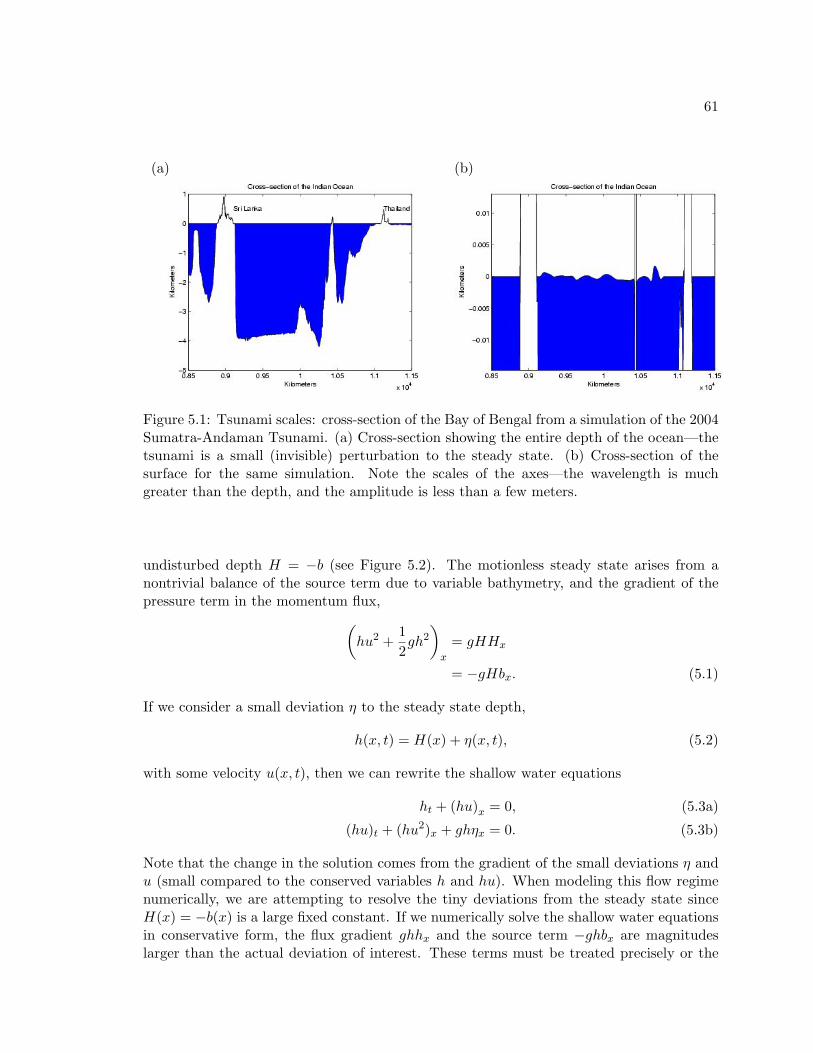
61

(a) (b)

Figure 5.1: Tsunami scales: cross-section of the Bay of Bengal from a simulation of the 2004Sumatra-Andaman Tsunami. (a) Cross-section showing the entire depth of the ocean—thetsunami is a small (invisible) perturbation to the steady state. (b) Cross-section of thesurface for the same simulation. Note the scales of the axes—the wavelength is muchgreater than the depth, and the amplitude is less than a few meters.

undisturbed depth H = −b (see Figure 5.2). The motionless steady state arises from anontrivial balance of the source term due to variable bathymetry, and the gradient of thepressure term in the momentum flux,(

hu2 +12gh2

)x

= gHHx

= −gHbx. (5.1)

If we consider a small deviation η to the steady state depth,

h(x, t) = H(x) + η(x, t), (5.2)

with some velocity u(x, t), then we can rewrite the shallow water equations

ht + (hu)x = 0, (5.3a)

(hu)t + (hu2)x + ghηx = 0. (5.3b)

Note that the change in the solution comes from the gradient of the small deviations η andu (small compared to the conserved variables h and hu). When modeling this flow regimenumerically, we are attempting to resolve the tiny deviations from the steady state sinceH(x) = −b(x) is a large fixed constant. If we numerically solve the shallow water equationsin conservative form, the flux gradient ghhx and the source term −ghbx are magnitudeslarger than the actual deviation of interest. These terms must be treated precisely or the

62

0←− η(x, t)

b(x)

H(x)

6

?

Figure 5.2: Deviation from the physically common steady state: a small perturbation ofamplitude η propagates against the background state with depth H(x) = −b(x). The figuredoes not depict a realistic scale, since for a real tsunami |η| << H.

solution of interest would be completely lost in noise. For instance, use of the fractionalstep methods described in Section 3.6, where the homogeneous shallow water equationsare solved by standard methods followed by an integration of the source term, would failmiserably for modeling this regime accurately—the numerical noise for typical grid spacingsmight be larger than the actual tsunami that we are trying to model!

It has been more standard practice in global tsunami modeling to use an alternativeform of the shallow water equations, using the non-conserved primitive variables,

ηt + ((η − b)u)x = 0, (5.4a)ut + uux + gηx = 0, (5.4b)

where η ≡ h+ b. The system (5.4) can be easily derived by manipulating the shallow waterequations in their conservative form. Note that for the motionless steady state, all of thegradients in (5.4) are zero. The motionless steady state balance has essentially been removedfrom the equations (5.4) by canceling terms after taking derivatives. Therefore, numericallypreserving the motionless steady state, or resolving small deviations to the steady state ismuch more easily accomplished. In fact, most standard finite difference methods based on

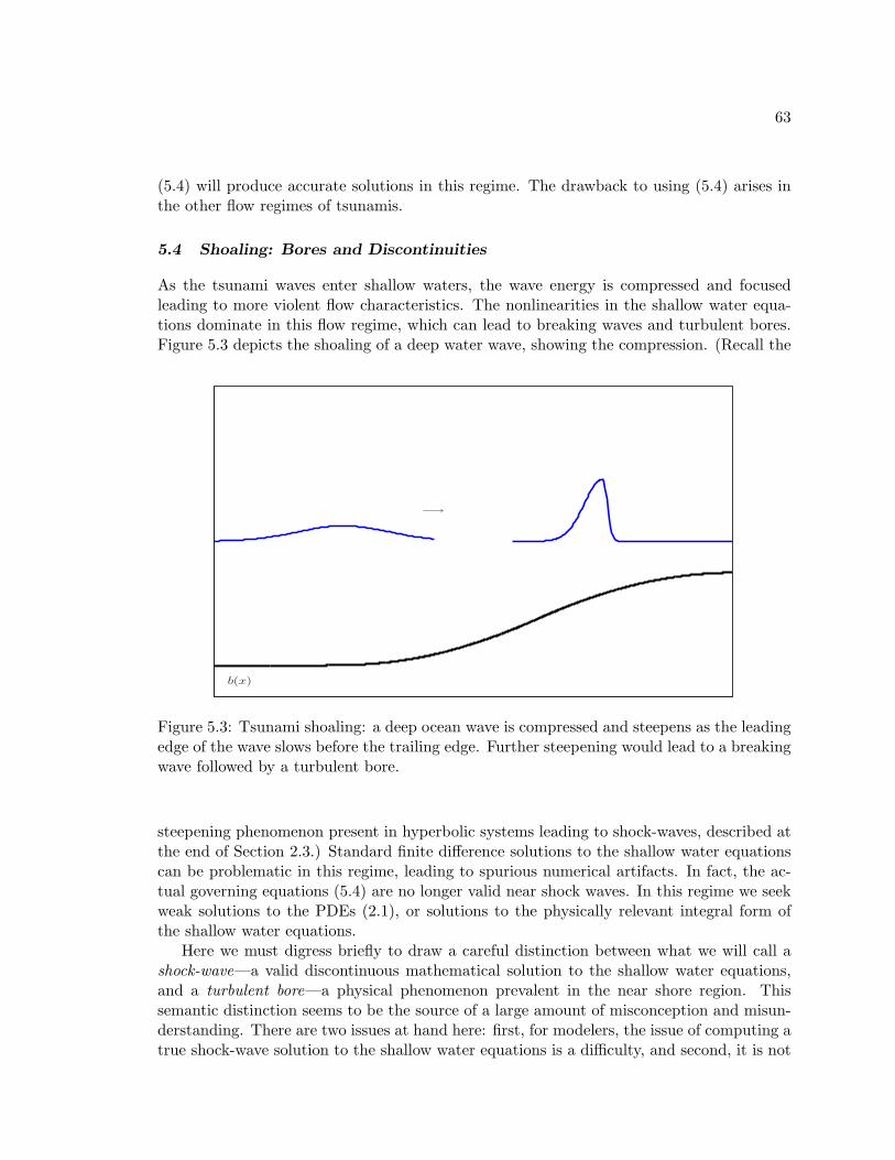
63

(5.4) will produce accurate solutions in this regime. The drawback to using (5.4) arises inthe other flow regimes of tsunamis.

5.4 Shoaling: Bores and Discontinuities

As the tsunami waves enter shallow waters, the wave energy is compressed and focusedleading to more violent flow characteristics. The nonlinearities in the shallow water equa-tions dominate in this flow regime, which can lead to breaking waves and turbulent bores.Figure 5.3 depicts the shoaling of a deep water wave, showing the compression. (Recall the

b(x)

−→

Figure 5.3: Tsunami shoaling: a deep ocean wave is compressed and steepens as the leadingedge of the wave slows before the trailing edge. Further steepening would lead to a breakingwave followed by a turbulent bore.

steepening phenomenon present in hyperbolic systems leading to shock-waves, described atthe end of Section 2.3.) Standard finite difference solutions to the shallow water equationscan be problematic in this regime, leading to spurious numerical artifacts. In fact, the ac-tual governing equations (5.4) are no longer valid near shock waves. In this regime we seekweak solutions to the PDEs (2.1), or solutions to the physically relevant integral form ofthe shallow water equations.

Here we must digress briefly to draw a careful distinction between what we will call ashock-wave—a valid discontinuous mathematical solution to the shallow water equations,and a turbulent bore—a physical phenomenon prevalent in the near shore region. Thissemantic distinction seems to be the source of a large amount of misconception and misun-derstanding. There are two issues at hand here: first, for modelers, the issue of computing atrue shock-wave solution to the shallow water equations is a difficulty, and second, it is not

64

clear how well a shock-wave solution to the shallow water equations represent the physicalturbulent bore or breaking wave. The resolution of the latter issue seems to be that shock-waves represent turbulent bores surprisingly well, if one considers only the macroscopicproperties of the bore, such as when it forms, its propagation speed, and how it affectsinundation (see [44, 97, 98, 108]). Certainly the shallow water equations do not describethe flow features right at the edge of the turbulent region of the bore. However, if the boreis represented mathematically as a discontinuity, the shallow water equations with appro-priate entropy conditions provide the correct conservation principles for hydrostatic flowsurrounding the bore. For the standard mathematical treatment of this topic, see [50],[87]or [103]. The empirical success of the shallow water equations is nicely summarized by Titovand Synolakis in [97]: “... further manifestation of the well-documented but unexplainedability of the shallow water wave equations to provide quantitatively correct runup resultseven in parameter ranges where the underlying assumptions of the governing equations areviolated.”

This work is more concerned with the first issue—numerically converging to correctdiscontinuous solutions of the shallow water equations. (Regardless of the crudeness of theshock-wave approximation to a true physical bore, certainly a correct solution to the shallowwater equations is a better approximation to the bore than a spurious one.) Shock-wavespose a difficulty for numerical solution for several reasons. First, PDE forms that are conve-nient for many of the flow regimes, such as (5.4), are no longer valid near discontinuities—only the physically relevant integral form of the shallow water equations provides the cor-rect formulation for a shock-wave. Second, nonconservative numerical methods, even thosebased on the physically conserved quantities, can converge to spurious discontinuous so-lutions propagating at incorrect speeds. And finally, discontinuities and steep gradientscan generate spurious oscillations in numerical methods that destroy accuracy, especiallyin standard finite difference methods that are based on the validity of Taylor series. It isnecessary to use a conservative numerical method that is based on the integral form of theshallow water equations, and use appropriate up-winding near shocks, such as that providedby solving Riemann problems, if we are to converge to correct weak solutions to the shallowwater equations. This creates a difficulty for modeling global propagation, as described inthe previous section.

5.5 Shorelines and Inundation

Ultimately, the goal of tsunami modeling is to determine what happens at the shoreline, sincethis is where tsunamis unleash their energy. The difficulties posed by the diverse regimesalready described are further exacerbated by the existence of dry regions and shorelines,especially if one attempts to model inundation. Inundation modeling poses several numericaldifficulties. First, the shoreline itself is a discontinuity, and methods based on PDEs mustuse some form of appropriate up-winding at this interface. Second, these regions havevanishing depths, and spurious negative solutions are a ubiquitous problem for numericalmethods in this regime. Third, it is not obvious how to determine the movement of theshoreline based on the flow variables and bathymetry near the shore, and rectifying accurateshore movement with positivity is difficult.

65

There are various types of approaches that have been used for treating the shoreline, themost common of which is to simply avoid inundation modeling by treating the shoreline asa fixed wall boundary. Inundation can then be estimated by runup at the boundary. Thisapproach is certainly not without merit, though it is less common recently since variousmethods for modeling inundation have become available. Most shoreline treatments mightbe referred to as shoreline-tracking methods. These methods attempt to track the shorelineexplicitly in some way, usually by a heuristic argument. Appropriate boundary conditions,or up-winding for finite difference methods, are then implemented near the shoreline. Someof the early shoreline-tracking methods can be found in [2] and [44]. A method developed byTitov and Synolakis [97], extrapolates the velocity of the fluid at the shoreline to determinethe movement and the position of the shoreline at the next time-step. Grid points areadded or removed appropriately, so that the computational grid covers the wet domain,with points right at the estimated shoreline. This method produces good comparison withanalytical solutions [97], and surprisingly good comparison with actual tsunami data [99, 96,98]—another testament to the use of the shallow water equations for inundation modeling.Another shoreline tracking method used by Knight, found in [70], extrapolates the surfaceelevation of the water near the shoreline in the direction perpendicular to linearly slopingbathymetry, as if water existed beyond the shoreline below the land. The location wherethe water surface intersects the land elevation after the time-step determines the shorelinelocation for the next time-step.

We will take a different approach, described more fully in the next chapter, by attempt-ing to capture the shoreline rather than explicitly track it. This is similar in philosophy tothe shock-capturing property of Godunov-type methods, where shocks are captured auto-matically by solving Riemann problems appropriately near these features.

66

Chapter 6

APPROXIMATE AUGMENTED RIEMANN SOLVERS FOR THESHALLOW WATER EQUATIONS AND TSUNAMI MODELING

Specialized Riemann solvers are one of the components that allow the finite volumemethods and the wave propagation algorithms to satisfy the requirements demanded bytsunami modeling—described in Chapter 5. For instance, Riemann solvers can be used toincorporate the source term from the shallow water equations directly into the updatingwaves, allowing accurate near-steady-state calculations required for transoceanic propaga-tion modeling. Additionally, Riemann solvers allow convergence to entropy satisfying dis-continuous solutions—the main impetus for which they were originally developed—allowingconvergence to solutions in regions that exhibit shocks and bores. Finally, dry regions andshorelines can be handled by developing Riemann solvers that maintain positivity, as wellas model the moving wet-dry interface directly—allowing inundation modeling. TypicalRiemann solvers, such as those introduced in Chapter 3, often deal with one or several ofthe above difficulties but often fail to handle all of the above difficulties simultaneously.

In this chapter, a novel Riemann solver will be described that we have developed todeal with the simultaneous difficulties described above. The Riemann solver will be shownto be well-balanced, a concept that will be described in Section 6.4. This will allow mod-eling the global propagation regime accurately, since the property implies that the wavesused in defining the numerical update represent deviations from the delicate steady state.The Riemann solver will also be shown to be depth-positive-definite as well as accurate atsolving the dry-state Riemann problem, making it appropriate for inundation modeling andshoreline capturing. Further, the solver is well suited for shock-capturing, and in fact willbe shown to be equivalent to the Roe solver near shocks. Lastly, the solver does not requirean entropy fix such as the Roe solver. It should be emphasized that although this particularsolver is novel, recently there has been considerable research directed toward developingsolvers with these properties (e.g. [26, 5]). However, the form of this solver is particularlywell suited for use with the wave propagation algorithms described in Chapter 3.

6.1 Augmented Systems

We can write the shallow water equations as a homogeneous hyperbolic system, by definingthe vector q to be the original conserved quantities q augmented by the bathymetry functionb,

q =

hhub

. (6.1)

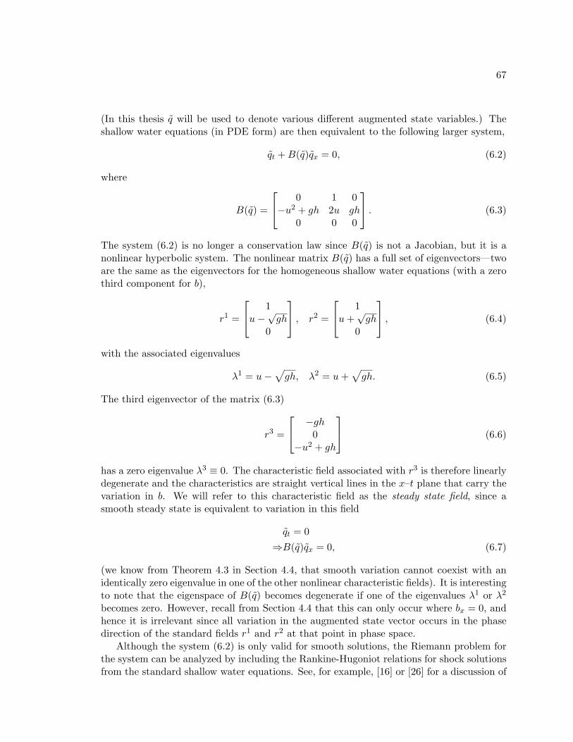
67

(In this thesis q will be used to denote various different augmented state variables.) Theshallow water equations (in PDE form) are then equivalent to the following larger system,

qt +B(q)qx = 0, (6.2)

where

B(q) =

0 1 0−u2 + gh 2u gh

0 0 0

. (6.3)

The system (6.2) is no longer a conservation law since B(q) is not a Jacobian, but it is anonlinear hyperbolic system. The nonlinear matrix B(q) has a full set of eigenvectors—twoare the same as the eigenvectors for the homogeneous shallow water equations (with a zerothird component for b),

r1 =

1u−

√gh

0

, r2 =

1u+

√gh

0

, (6.4)

with the associated eigenvalues

λ1 = u−√gh, λ2 = u+

√gh. (6.5)

The third eigenvector of the matrix (6.3)

r3 =

−gh0

−u2 + gh

(6.6)

has a zero eigenvalue λ3 ≡ 0. The characteristic field associated with r3 is therefore linearlydegenerate and the characteristics are straight vertical lines in the x–t plane that carry thevariation in b. We will refer to this characteristic field as the steady state field, since asmooth steady state is equivalent to variation in this field

qt = 0⇒B(q)qx = 0, (6.7)

(we know from Theorem 4.3 in Section 4.4, that smooth variation cannot coexist with anidentically zero eigenvalue in one of the other nonlinear characteristic fields). It is interestingto note that the eigenspace of B(q) becomes degenerate if one of the eigenvalues λ1 or λ2

becomes zero. However, recall from Section 4.4 that this can only occur where bx = 0, andhence it is irrelevant since all variation in the augmented state vector occurs in the phasedirection of the standard fields r1 and r2 at that point in phase space.

Although the system (6.2) is only valid for smooth solutions, the Riemann problem forthe system can be analyzed by including the Rankine-Hugoniot relations for shock solutionsfrom the standard shallow water equations. See, for example, [16] or [26] for a discussion of

68

some properties of systems such as (6.2). Of course, unlike Riemann problems for homoge-neous integral conservation laws, (6.2) is not classically defined for problems where part ofthe solution (b(x)) is non-differentiable. For this system, the Riemann problem might betterbe thought of as an approximation to a slightly smoothed problem. For a more rigorousdiscussion involving more generalized functions, see [35]. Augmented systems that elimi-nate the source term by introducing an additional variable and nonconservative productsare described more generally in [10]. Some methods for the shallow water equations withbathymetry that include additional solution variables and transformations of the solutionvariables are described in [26].

An additional augmented system can be derived by first considering a governing equationfor the flux of a hyperbolic conservation law. Consider a general hyperbolic conservationlaw (with source term)

qt + f(q)x = ψ(q, x). (6.8)

Multiplying (6.8) by the Jacobian f ′(q) gives

f ′(q)qt + f ′(q)f(q)x = f ′(q)ψ(q, x). (6.9)

By noting that f ′(q)qt = f(q)t, equation (6.9) implies a hyperbolic system for the flux f(q),

ft + f ′(q)fx = f ′(q)ψ(q, x), (6.10)

where the dependence of f on q has been dropped. For the shallow water equations, whereq2 = f1, the first equation of (6.10) simply reproduces the momentum equation for theshallow water equations. The second equation in (6.10) is a governing equation for f2 =φ = (hu2 + 1

2gh2), which can be written as

φt + (−u2 + gh)(hu)x + (2u)φx + (2ugh)bx = 0. (6.11)

Of course, the flux is entirely determined by the solution to the shallow water equations,but (6.11) will provide some theoretical insight into how the flux behaves. By defining theadditional augmented state variable (first introduced in Section 4.4)

q =

hhuφb

, (6.12)

and including equation (6.11), the shallow water equations can be written as an overdeter-mined, augmented homogeneous system

qt + B(q)qx = 0, (6.13)

where

B(q) =

0 1 0 0

−u2 + gh 2u 0 gh0 −u2 + gh 2u 2ugh0 0 0 0

. (6.14)

69

The matrix B(q) has the eigenvectors

r1 =

1

u−√gh(

u−√gh)2

0

, r2 =

1

u+√gh(

u+√gh)2

0

, r3 =

0010

, r4 =

−gh

−u2+gh

0−gh

1

, (6.15)

with associated eigenvalues

λ1 = u−√gh, λ2 = u+

√gh, λ3 = 2u, λ4 = 0. (6.16)

Note that r1 and r2 correspond to the nonlinear fields associated with the standard shallowwater equations. The field associated with r4 is the linearly degenerate steady state fielddescribed in the preceding discussion, yet now the vector also dictates how the flux φ shouldvary through the steady state field. The eigenvector r3 has a nonzero component only inthe “direction” (in phase space) of φ. This field is physically irrelevant, since the flux is onlya function of h and hu, and cannot vary independently. Since the system (6.13) is valid forsmooth solutions, it must be that solutions to the shallow water equations are never simplewaves corresponding to this field. This is confirmed if we note that through any simple wave

f(q)x = f ′(q)qx = c(x)λprp, (6.17)

for p = 1, 2, and some scalar function c(x). Considering the eigenstructure for the shallowwater equations, (6.17) implies that through a simple wave of the first or second family,

∂

∂x

hhuφ

= c(x)

1λp

(λp)2

, (6.18)

where (λp)2 is the pth eigenvalue squared. Although nonphysical, we might heuristicallyinterpret r3 as a field that would carry variation in the flux φ if it was another variableindependent of h and hu.

6.2 An Approximate Riemann Solver Based on an Augmented System

In this section we will introduce an approximate Riemann solver, before describing itsfeatures more fully in the following sections while showing its relation to various otherRiemann solvers. It is hoped that this solver will be viewed as unifying many of the strengthsof several solvers with diverse properties. The solver is introduced first in a simplified basicform, before describing some corrections in the sections that follow that supply some addedproperties.

Given a Riemann problem for the shallow water equations, we consider the correspondingRiemann problem for the augmented system (6.13),

qt + B(q)qx = 0, (6.19a)

70

with piecewise constant initial data

q(x, 0) =

ql if x < 0qr if x > 0

, (6.19b)

where, of course,

ql =

hl

(hu)lφlbl

, and qr =

hr

(hu)rφrbr

. (6.19c)

We then approximate the solution to (6.19), by the decomposition

∆q = qr − ql =4∑p=1

αprp, (6.20a)

where rp are local approximations to the eigenvectors of B,

r1 =

1s1E

(s1E)2

0

, r2 =

1s2E

(s2E)2

0

, r3 =

0010

, r4 =

S+−(ql,qr)

−λ1λ2(ql,qr)

0S+− (ql, qr)

1

. (6.20b)

The values s1,2E are the Einfeldt speeds defined in Section 3.3, and S+− (ql, qr) and λ1λ2(ql, qr)

are the averages defined in Section 4.4. We then propagate the waves defined by the de-composition at speeds

s1 = s1E , s2 = s2E , s3 =12(s1E + s2E), s4 = 0. (6.20c)

The third eigenpair, r3 and s3, are only one of several options presented here for complete-ness. Properties of this eigenpair and other options will be discussed in Section 6.7 when wediscuss entropy fixes. We will refer to (6.20) as an augmented approximate Riemann solver.

Note that we only need two components of the waves defined by (6.20) in order to updatethe solution. In order to maintain conservation, we will use the waves associated with theflux components to update the solution directly, based on the f -wave method described inChapter 3. This will be described more in Section 6.4.

A Riemann solver that decomposes an augmented variable, such as that defined by (6.20),can be related to simple relaxation schemes such as those described in [49]. This connectionis described by LeVeque and Pelanti [69] and also in the text [10]. These connections arenot further explored here.

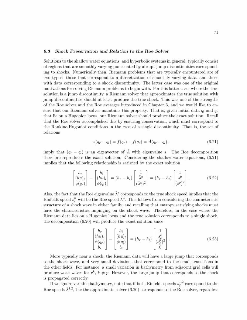
71

6.3 Shock Preservation and Relation to the Roe Solver

Solutions to the shallow water equations, and hyperbolic systems in general, typically consistof regions that are smoothly varying punctuated by abrupt jump discontinuities correspond-ing to shocks. Numerically then, Riemann problems that are typically encountered are oftwo types: those that correspond to a discretization of smoothly varying data, and thosewith data corresponding to a shock discontinuity. The latter case was one of the originalmotivations for solving Riemann problems to begin with. For this latter case, where the truesolution is a jump discontinuity, a Riemann solver that approximates the true solution withjump discontinuities should at least produce the true shock. This was one of the strengthsof the Roe solver and the Roe averages introduced in Chapter 3, and we would like to en-sure that our Riemann solver maintains this property. That is, given initial data ql and qrthat lie on a Hugoniot locus, our Riemann solver should produce the exact solution. Recallthat the Roe solver accomplished this by ensuring conservation, which must correspond tothe Rankine-Hugoniot conditions in the case of a single discontinuity. That is, the set ofrelations

s(qr − ql) = f(qr)− f(qr) = A(qr − ql), (6.21)

imply that (qr − ql) is an eigenvector of A with eigenvalue s. The Roe decompositiontherefore reproduces the exact solution. Considering the shallow water equations, (6.21)implies that the following relationship is satisfied by the exact solution hr

(hu)rφ(qr)

− hl

(hu)lφ(ql)

= (hr − hl)

1λp

(λp)2

= (hr − hl)

1sp

(sp)2

. (6.22)

Also, the fact that the Roe eigenvalue λp corresponds to the true shock speed implies that theEinfeldt speed spE will be the Roe speed λp. This follows from considering the characteristicstructure of a shock wave in either family, and recalling that entropy satisfying shocks musthave the characteristics impinging on the shock wave. Therefore, in the case where theRiemann data lies on a Hugoniot locus and the true solution corresponds to a single shock,the decomposition (6.20) will produce the exact solution since

hr(hu)rφ(qr)br

−

hl(hu)lφ(ql)bl

= (hr − hl)

1spE

(spE)2

0

. (6.23)

More typically near a shock, the Riemann data will have a large jump that correspondsto the shock wave, and very small deviations that correspond to the small transitions inthe other fields. For instance, a small variation in bathymetry from adjacent grid cells willproduce weak waves for rk, k 6= p. However, the large jump that corresponds to the shockis propagated correctly.

If we ignore variable bathymetry, note that if both Einfeldt speeds s1,2E correspond to theRoe speeds λ1,2, the the approximate solver (6.20) corresponds to the Roe solver, regardless

72

of the form of r3. This is because the jump in q lies in the two dimensional space spannedby

1λ1

(λ1)2

0

, and

1λ2

(λ2)2

0

, (6.24)

which follows from the conservative property of the Roe solver:

f(qr)− f(ql) = A(qr − ql) = A2∑p=1

αprp =2∑p=1

αpλprp. (6.25)

Considering the shallow water equations, (6.25) implies that hr(hu)rφ(qr)

− hl

(hu)lφ(ql)

=2∑p=1

αp

1λp

(λp)2

. (6.26)

Therefore, the decomposition (6.20) would result in α3 = 0. For typical Riemann problemsthat correspond to discretized smooth data, or perhaps shocks, we expect |α3| << |αp|,p 6= 3, since, if one of the Einfeldt speeds is not the Roe speed the two will typically be veryclose. An exception occurs in the case of a strong rarefaction, where either ul−

√ghl << λ1

or ur +√ghr >> λ2. This will be explored more fully when we discuss entropy fixes and

strong rarefactions in Section 6.7.

6.4 Source Terms and Well-Balancing

In Section 5.3 it was shown that accuracy for tsunami modeling will require our numericalmethod to perfectly preserve certain steady states, and more importantly, resolve tiny de-viations to the steady state. The steady state arises from a nontrivial balance of the sourceterm and the flux gradient, as described in Chapter 4 and Chapter 5. At first glance itmight seem that the Riemann solver defined by (6.20) does not include the source term,since it does not appear in the variables decomposed into the propagating waves. However,recall that our numerical update comes from the re-averaging effect of waves moving intothe grid cells and second order corrections based on those waves. The wave associated withthe linearly degenerate steady state field, r4, is a contact discontinuity that remains at x = 0producing the contribution of the source term.

6.4.1 Relation to the f-wave Method

In Section 3.3 the f -wave method was introduced as an approach for dealing with problemswhere the solution is discontinuous at the cell interfaces, either due to a variable coefficientflux function, or in the case described in Section 3.6, due to a point source terms concentrated

73

at the cell interfaces. In this latter case, recall that the point source term is accounted forby subtracting it from the flux function before performing the decomposition

f(qr)− f(ql)−Ψ∆x =Mw∑p=1

βprp, (6.27)

where Ψ∆x is some approximation of the source term,∫ xr

xlψ dx, and rp, p = 1, · · · ,Mw,

are some set of suitable approximations to the eigenvectors of the Jacobian. The resultingwaves Zp = βprp moving into the surrounding grid cells then update the solution directly.For the shallow water equations, (6.27) takes the form[

(hu)r − (hu)lφr − φl −

∫ xr

xlψ dx

]=

2∑p=1

βp[

1λp

], (6.28)

where∫ xr

xlψ dx is some approximation to −

∫ xr

xlghbx dx, based on ql,bl,br and qr, and λp

are approximations to the eigenvalues of the Jacobian. If we now consider the augmenteddecomposition (6.20), it must be that α4 = (br − bl), since this is the only eigenvector witha nonzero fourth component. Therefore, ultimately the decomposition is equivalent to thatobtained by first subtracting (br − bl)r4 from q, followed by a decomposition of the firstthree components of q onto the first three components of the remaining eigenvectors. If weconsider just the flux components of such a decomposition, which are what get used for thenumerical update, we have[

(hu)r − (hu)lφr − φl − S+

− (ql, qr)(br − bl)

]=

2∑p=1

αpspE

[1spE

]+ β3r3. (6.29)

Since S+− (ql, qr)(br − bl) is an approximation to

∫ xr

xl−ghbx dx, as shown in Section 4.4,

equation (6.29) elucidates the relation between the standard f -wave approach, equation(6.28), and the augmented decomposition (6.20). Note that the form of r4 and the firstcomponent of q—the depth h—ultimately determine the difference since they affect thedecomposition of the flux into the three vectors in (6.29) rather than the two in (6.28).

6.4.2 Well-Balancing and Preservation of Steady States

A well-balanced method generally is one that perfectly preserves certain discrete steady statedata. That is, if we take a smooth steady state solution to a hyperbolic conservation lawwith a source term, and use some relevant spatial discretization of that solution for an initialcondition, a well-balanced method will have an identically zero numerical update. Oftena method might be referred to as well-balanced even if it preserves only certain importantsteady states. For instance, various well-balanced schemes have been developed for the“lake at rest” Riemann problem for the shallow water equations, where ul = ur = 0, andhl+ bl = hr + br (e.g. [5, 12, 27, 77]). For a discussion of well-balanced schemes in the moregeneral context of hyperbolic systems with source terms see the work of Greenberg, LeRouxet al [38, 39], or the recent text [10] by Bouchut.

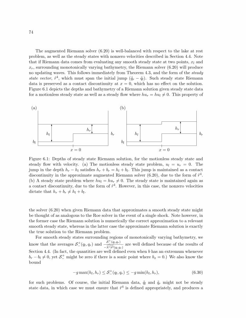
74

The augmented Riemann solver (6.20) is well-balanced with respect to the lake at restproblem, as well as the steady states with nonzero velocities described in Section 4.4. Notethat if Riemann data comes from evaluating any smooth steady state at two points, xl andxr, surrounding monotonically varying bathymetry, the Riemann solver (6.20) will produceno updating waves. This follows immediately from Theorem 4.3, and the form of the steadystate vector, r4, which must span the initial jump (qr − ql). Such steady state Riemanndata is preserved as a contact discontinuity at x = 0, which has no effect on the solution.Figure 6.1 depicts the depths and bathymetry of a Riemann solution given steady state datafor a motionless steady state as well as a steady flow where hur = hul 6= 0. This property of

(a) (b)

x = 0

bl

hl

6

?

brhr

6

?

x = 0

bl

hl

6

?

br

hr6

?

Figure 6.1: Depths of steady state Riemann solution, for the motionless steady state andsteady flow with velocity. (a) The motionless steady state problem, ul = ur = 0. Thejump in the depth hr − hl satisfies hr + br = hl + bl. This jump is maintained as a contactdiscontinuity in the approximate augmented Riemann solver (6.20), due to the form of r4.(b) A steady state problem where hul = hur 6= 0. The steady state is maintained again asa contact discontinuity, due to the form of r4. However, in this case, the nonzero velocitiesdictate that hr + br 6= hl + bl.

the solver (6.20) when given Riemann data that approximates a smooth steady state mightbe thought of as analogous to the Roe solver in the event of a single shock. Note however, inthe former case the Riemann solution is numerically the correct approximation to a relevantsmooth steady state, whereas in the latter case the approximate Riemann solution is exactlythe true solution to the Riemann problem.

For smooth steady states surrounding regions of monotonically varying bathymetry, we

know that the averages S+− (ql, qr) and

S+−(ql,qr)

−λ1λ2(ql,qr)are well defined because of the results of

Section 4.4. (In fact, the quantities are well defined even when b has an extremum wheneverbr − bl 6= 0, yet S+

− might be zero if there is a sonic point where bx = 0.) We also know thebound

−gmax(hl, hr) ≤ S+− (ql, qr) ≤ −gmin(hl, hr), (6.30)

for such problems. Of course, the initial Riemann data, ql and qr might not be steadystate data, in which case we must ensure that r4 is defined appropriately, and produces a

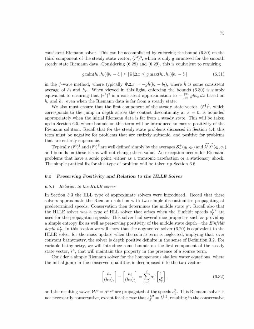
75

consistent Riemann solver. This can be accomplished by enforcing the bound (6.30) on thethird component of the steady state vector, (r4)3, which is only guaranteed for the smoothsteady state Riemann data. Considering (6.28) and (6.29), this is equivalent to requiring

gmin(hl, hr)|br − bl| ≤ |Ψ|∆x ≤ gmax(hl, hr)|br − bl| (6.31)

in the f -wave method, where typically Ψ∆x = −gh(br − bl), where h is some consistentaverage of hl and hr. When viewed in this light, enforcing the bounds (6.30) is simplyequivalent to ensuring that (r4)3 is a consistent approximation to −

∫ xr

xlghbx dx based on

hl and hr, even when the Riemann data is far from a steady state.We also must ensure that the first component of the steady state vector, (r4)1, which

corresponds to the jump in depth across the contact discontinuity at x = 0, is boundedappropriately when the initial Riemann data is far from a steady state. This will be takenup in Section 6.5, where bounds on this term will be introduced to ensure positivity of theRiemann solution. Recall that for the steady state problems discussed in Section 4.4, thisterm must be negative for problems that are entirely subsonic, and positive for problemsthat are entirely supersonic.

Typically (r4)1 and (r4)3 are well defined simply by the averages S+− (ql, qr) and λ1λ2(ql, qr),

and bounds on these terms will not change there value. An exception occurs for Riemannproblems that have a sonic point, either as a transonic rarefaction or a stationary shock.The simple pratical fix for this type of problem will be taken up Section 6.6.

6.5 Preserving Positivity and Relation to the HLLE Solver

6.5.1 Relation to the HLLE solver

In Section 3.3 the HLL type of approximate solvers were introduced. Recall that thesesolvers approximate the Riemann solution with two simple discontinuities propagating atpredetermined speeds. Conservation then determines the middle state q∗. Recall also thatthe HLLE solver was a type of HLL solver that arises when the Einfeldt speeds s1,2E areused for the propagation speeds. This solver had several nice properties such as providinga simple entropy fix as well as preserving positivity of the middle state depth—the Einfeldtdepth h∗E . In this section we will show that the augmented solver (6.20) is equivalent to theHLLE solver for the mass update when the source term is neglected, implying that, overconstant bathymetry, the solver is depth positive definite in the sense of Definition 3.2. Forvariable bathymetry, we will introduce some bounds on the first component of the steadystate vector, r4, that will maintain this property in the presence of a source term.

Consider a simple Riemann solver for the homogeneous shallow water equations, wherethe initial jump in the conserved quantities is decomposed into the two vectors[

hr(hu)r

]−[hl

(hu)l

]=

2∑p=1

αp[

1spE

], (6.32)

and the resulting waves Wp = αprp are propagated at the speeds spE . This Riemann solver isnot necessarily conservative, except for the case that s1,2E = λ1,2, resulting in the conservative

76

Roe solver. However, considering the re-averaging effect of the first component of thepropagating waves W1,2, conservation of mass requires

α1s1E + α2s2E = (hu)r − (hu)l. (6.33)

Since this condition is exactly the second equation of (6.32), the method must conservemass. Note also that since the second component of each vector rp corresponds to the speedof the wave, using the jump in depth multiplied by speed of the moving discontinuity todefine the update to the mass equation—as in the standard wave propagation algorithm—must be the same as using the jumps in the momentum directly to update the mass—asin the f -wave approach. Therefore, the two effective middle state depths (Definition 3.1)implied by the second equation in (6.32) are equivalent to the actual single middle statedepth implied by the first equation. Stated more broadly, a consistent use of the first orsecond equation in (6.32) to update the mass equation produces the same numerical result.

Since the HLLE method conserves mass with only two jump discontinuities propagatingat the same speeds as (6.32), the HLLE method and (6.32) must be identical for the masscomponent. (This can be further verified—the mass decomposition in (6.32) implies amiddle state depth h∗, where, α1 = hr−h∗ and α2 = h∗−hl. Therefore, (6.33) is equivalentto (3.26)—the equation that defines h∗E from Theorem 3.1.) Since we saw that the HLLEmethod preserves positivity of depth from Theorem 3.1, the method implied by (6.32) mustalso preserve positivity in the sense of Definition 3.1.

6.5.2 Preserving Positivity with the Augmented Decomposition

For the augmented decomposition (6.20), the initial jump qr − ql is ultimately decomposedinto four vectors, representing four propagating discontinuities or waves. Writing the de-composition in (6.20) as

hr

(hu)r∗∗

−

hl(hu)l∗∗

=

1 1 0

S+−(ql,qr)

−λ1λ2(ql,qr)

s1E s2E 0 0∗ ∗ ∗ ∗∗ ∗ ∗ ∗

α1

α2

α3

α4

, (6.34)

allows us to concentrate on the depth and momentum components of the decomposition.For the case of constant bathymetry, where br − bl = α4 = 0, it is clear that (6.34) isidentical to the decomposition (6.32) for depth and momentum. Like the HLLE methodthen, when there is constant bathymetry our method (6.20) must preserve positivity ofdepth in the sense of Definition 3.2. Of course, once variable bathymetry is introduced tothe Riemann problem, there exists a jump in depth at x = 0 due to a nonzero α4, therebychanging the terms α1 and α2, and creating two middle state depths—h∗l and h∗r . SeeFigure 6.2 depicting such an approximate Riemann solution. Recall from Section 3.3, whereit was shown that the existence of two effective middle state depths, h∗l and h∗r , preventedmaintaining effective positivity when using the f -wave approach, where the momentumdecomposition alone updated the mass equation. However, decomposing both the depthand momentum in the augmented decomposition (6.20), will allow us to control the effective

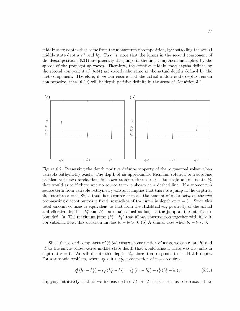
77

middle state depths that come from the momentum decomposition, by controlling the actualmiddle state depths h∗l and h∗r . That is, note that the jumps in the second component ofthe decomposition (6.34) are precisely the jumps in the first component multiplied by thespeeds of the propagating waves. Therefore, the effective middle state depths defined bythe second component of (6.34) are exactly the same as the actual depths defined by thefirst component. Therefore, if we can ensure that the actual middle state depths remainnon-negative, then (6.20) will be depth positive definite in the sense of Definition 3.2.

(a) (b)

x = 0 s2

E∆ts1

E∆t

h∗E

h∗l

hr

hl

x = 0 s2

E∆ts1

E∆t

h∗E

h∗r

hr

hl

Figure 6.2: Preserving the depth positive definite property of the augmented solver whenvariable bathymetry exists. The depth of an approximate Riemann solution to a subsonicproblem with two rarefactions is shown at some time t > 0. The single middle depth h∗Ethat would arise if there was no source term is shown as a dashed line. If a momentumsource term from variable bathymetry exists, it implies that there is a jump in the depth atthe interface x = 0. Since there is no source of mass, the amount of mass between the twopropagating discontinuities is fixed, regardless of the jump in depth at x = 0 . Since thistotal amount of mass is equivalent to that from the HLLE solver, positivity of the actualand effective depths—h∗l and h∗r—are maintained as long as the jump at the interface isbounded. (a) The maximum jump (h∗r − h∗l ) that allows conservation together with h∗r ≥ 0.For subsonic flow, this situation implies br − bl > 0. (b) A similar case when br − bl < 0.

Since the second component of (6.34) ensures conservation of mass, we can relate h∗l andh∗r to the single conservative middle state depth that would arise if there was no jump indepth at x = 0. We will denote this depth, h∗E , since it corresponds to the HLLE depth.For a subsonic problem, where s1E < 0 < s2E , conservation of mass requires

s2E (hr − h∗E) + s1E (h∗E − hl) = s2E (hr − h∗r) + s1E (h∗l − hl) , (6.35)

implying intuitively that as we increase either h∗l or h∗r the other must decrease. If we

78

increase h∗r until h∗l = 0, (6.35) implies that

h∗r =(s2E − s1E)

s2Eh∗E . (6.36)

Similarly, if h∗r = 0, we have

h∗l =(s2E − s1E)−s1E

h∗E . (6.37)

If we prevent h∗l or h∗r from becoming negative, then (6.36) and (6.37) imply a bound onh∗r − h∗l ,

(s2E − s1E)s1E

h∗E ≤ h∗r − h∗l ≤(s2E − s1E)

s2Eh∗E . (6.38)

Since, the method (6.20) implies

h∗r − h∗l = (br − bl)(r4)1, (6.39)

(6.38) would be satisfied if

(s2E − s1E)s1E

h∗E ≤ (br − bl)(r4)1 ≤(s2E − s1E)

s2Eh∗E . (6.40)

Note that the first term in (6.40) is negative and the last is positive for subsonic flow.Since (r4)1 is an approximation to

(−gh/(−λ1λ2)

), we expect this term to be negative for

subsonic flow and positive for supersonic flow. For steady state problems, we know that(r4)1 will be appropriately defined by

(r4)1 =S+− (ql, qr)

−λ1λ2(ql, qr). (6.41)

However, for subsonic problems that are far from a steady state, we may need to bound(r4)1 by the conditions,

(s2E − s1E)s1E

h∗E(br − bl)

≤(r4)1 ≤ −1 if br − bl > 0, (6.42a)

(s2E − s1E)s2E

h∗E(br − bl)

≤(r4)1 ≤ −1 if br − bl < 0, (6.42b)

These bounds will ensure that the middle state depths are positive in the case of subsonicflow.

For supersonic flow, we expect (r4)1 to change sign, however, bounding this term is notnecessary for guaranteeing positivity since all of the waves move in one direction. This isbecause conservation of mass ensures that multiple middle state depths arising from themultiple waves integrate to the single nonnegative middle state depth, h∗E . Since all of the

79

waves move in the same direction, the numerical effect of a negative middle state depth isbalanced by a positive one. In fact, the term (r4)1 has no effect on the numerical solutionat all for supersonic flow, at least when considering the first order update. (Since limitersapplied to second-order corrections are based on comparing individual wave families fromadjacent cells, bounding the term (r4)1 for supersonic flow may have some unforeseen benefit,since it would change the weights in the decomposition (6.20) into different wave families.This has not yet been explored, however, the bounds that prevent negative middle statedepths are easily determined.) To maintain positivity of all of actual and effective middlestate depths, using arguments similar to those above for subsonic problems, the followingbounds suffice:

0 ≤(r4)1 ≤ s2E − s1E

s1E

h∗E(br − bl)

if br − bl > 0, (6.43a)

0 ≤(r4)1 ≤ −hl

(br − bl)if br − bl < 0, (6.43b)

when 0 < s1E < s2E , and

0 ≤(r4)1 ≤ hr

(br − bl)if br − bl > 0, (6.44a)

0 ≤(r4)1 ≤ s2E − s1E

s2E

h∗E(br − bl)

if br − bl < 0, (6.44b)

when s1E < s2E < 0.

80

6.6 The Resonant Problem and Near-Sonic Problems

In defining the steady state vector r4 for the augmented solver, it has been assumed that allof the averages used for the components are well defined. For problems that are subsonic,λ1λ2(ql, qr) and λ1λ2(ql, qr) are negative, and S+

− (ql, qr) is a consistent approximation for

−gh. The same is true for supersonic problems, accept that λ1λ2(ql, qr) and λ1λ2(ql, qr)are each positive. This reflects the fact that for steady subsonic problems, hx and bx haveopposite signs and for steady supersonic problems they have the same sign. However, it ispossible to have Riemann problems where either λ1λ2(ql, qr) and λ1λ2(ql, qr) are oppositein sign or perhaps one is zero. This problem can be better understood by considering theaugmented system discussed in Section 6.1. Note that if one of the eigenvalues λ1(q) or λ2(q)passes through zero, the corresponding eigenvector r1(q) or r2(q) (in (6.4)) is identical to thesteady state eigenvector r3(q) (in (6.6)), and a full set of linearly independent eigenvectors nolonger exists. Therefore, at such a point, there is no eigenvector with a component allowingvariation in the additional variable b. This is a more general problem for augmented systemswhere a nonhomogeneous system is converted to a homogeneous one with nonconservativeproducts, such as (6.2). This is known as the resonant problem, and it is discussed in moredetail in [16]. In Section 6.1, it was pointed out that this is not relevant for exact physicalsolutions, since a sonic point cannot occur over variable bathymetry, and must occur atan extremum in b. However, it is possible to encounter Riemann problems with data thatresults in a critical point in the homogeneous solution, together with a jump in (br − bl).For instance, if a steady state with a critical point at a local extremum in b is discretized,such a Riemann problem might result. For such a problem, recall from Section 4.4, that bxand hx are of the same sign to one side of the critical point and opposite sign to the other.The same relationship exists for a stationary shock over smoothly varying bathymetry. Forthe resulting Riemann problems, the relationship between (hr−hl) and (br− bl), and hencethe sign of (r4)1, is unclear.

We can deal with problems where the standard definitions used in r4 are inconsistent, bysimply checking if the problem has data that reflects a possible sonic point. In such a case,(r4)1 is set to zero, and S+

− (qr, ql) is defined as −gh. A simple sonic check can be performed

by simply looking at the quantities, λ1(ql)λ1(qr), λ2(ql)λ2(qr) and λ1λ2(ql, qr)λ1λ2(ql, qr).If any of these quantities is less than or equal to zero, the Riemann data contains a sonicpoint. In practice it makes sense to compare the sign of λ1λ2 and λ1λ2 with the sign of s1Es

2E ,

so that for subsonic or supersonic problems, all of the definitions used in the eigenvectorsare consistent with the direction that the waves propagate.

Perhaps fortuitously, the two dimensional space spanned by r4 and rk does not dependon (r4)1, when skE = 0. Therefore, setting (r4)1 = 0 has no effect on the approximatesolution for problems where skE is zero—a portion of the jump (qr− ql) is projected onto thistwo-dimensional space, and these two waves remain at the interface. Considering (4.94),the space spanned by r4 and rk approximates the true jump in the steady state solutionwhen there is a stationary shock in the kth family over variable bathymetry.

81

6.7 Rarefactions and Entropy Fixes

In this section we will discuss alternatives for the approximate eigenvector r3 used in theRiemann solver (6.20). Although the Einfeldt speeds provide an entropy fix for the patholog-ical expansion shock, which can result from trancritical rarefactions, these large speeds canproduce approximate solutions with poor accuracy for these and similar types of Riemannproblems. It will be shown that the vector r3 can be used to produce better numericalapproximation for Riemann problems with strong, possibly transcritical rarefactions. Inthis section we will consider Riemann solutions to the homogeneous shallow water equa-tions with no variable bathymetry, since Riemann problems with large transitions in thetwo nonlinear fields are our main concern here.

6.7.1 The Commonly Encountered Riemann Problem and Weak Transitions

When the augmented decomposition (6.20) was introduced in Section 6.2, it included

r3 =[0 0 1 0

]T, (6.45)

as an additional eigenvector in the decomposition of (qr−ql). This is in fact an eigenvector ofthe augmented system (6.3), but as pointed out in Section 6.1, this eigenvector is nonphysicalsince the flux φ is a function only of h and hu. For smooth solutions, f(q)x = f ′(q)qx,therefore, at any point the vector hhu

φ

x

, (6.46)

must lie in the two dimensional space spanned by 1λ1(q)

(λ1(q))2

, 1λ2(q)

(λ2(q))2

. (6.47)

As described in Section 6.3, solutions to hyperbolic conservation laws typically haveregions with smooth variation in the solution, punctuated by abrupt shock wave disconti-nuities. If we consider a discretized smooth solution, evaluated at two points xl and xr withxr − xl = ∆x, using Taylor series it is easy to show that hhu

φ

r

−

hhuφ

l

=2∑1

αp

1λp

(λp)2

+O(∆x2), (6.48)

where λp is any consistent approximation to λp(q) based on ql and qr. For typical Riemannproblems in smooth varying regions, spE ≈ λp(ql) ≈ λp(qr), and for the decomposition hhu

φ

r

−

hhuφ

l

=

1 0 1s1E s2E 0

(s1E)2 (s2E)

2 1

α1

α2

α3

, (6.49)

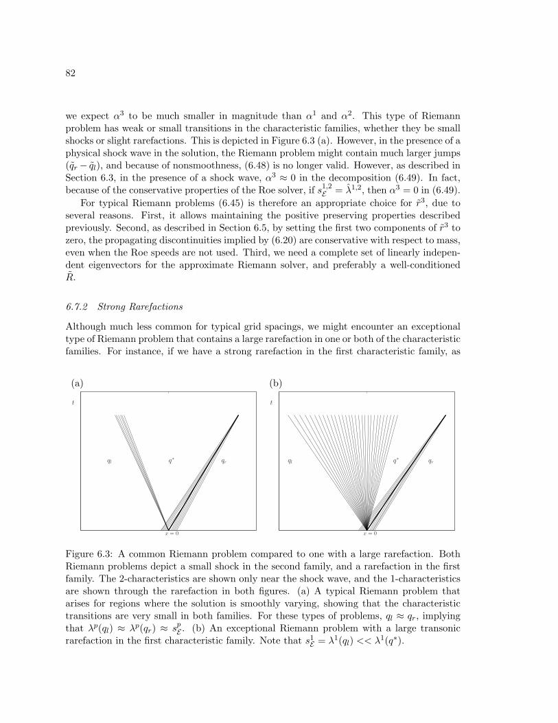
82

we expect α3 to be much smaller in magnitude than α1 and α2. This type of Riemannproblem has weak or small transitions in the characteristic families, whether they be smallshocks or slight rarefactions. This is depicted in Figure 6.3 (a). However, in the presence of aphysical shock wave in the solution, the Riemann problem might contain much larger jumps(qr − ql), and because of nonsmoothness, (6.48) is no longer valid. However, as described inSection 6.3, in the presence of a shock wave, α3 ≈ 0 in the decomposition (6.49). In fact,because of the conservative properties of the Roe solver, if s1,2E = λ1,2, then α3 = 0 in (6.49).

For typical Riemann problems (6.45) is therefore an appropriate choice for r3, due toseveral reasons. First, it allows maintaining the positive preserving properties describedpreviously. Second, as described in Section 6.5, by setting the first two components of r3 tozero, the propagating discontinuities implied by (6.20) are conservative with respect to mass,even when the Roe speeds are not used. Third, we need a complete set of linearly indepen-dent eigenvectors for the approximate Riemann solver, and preferably a well-conditionedR.

6.7.2 Strong Rarefactions

Although much less common for typical grid spacings, we might encounter an exceptionaltype of Riemann problem that contains a large rarefaction in one or both of the characteristicfamilies. For instance, if we have a strong rarefaction in the first characteristic family, as

(a) (b)

x = 0

t

q∗ qrql

x = 0

t

q∗ qrql

Figure 6.3: A common Riemann problem compared to one with a large rarefaction. BothRiemann problems depict a small shock in the second family, and a rarefaction in the firstfamily. The 2-characteristics are shown only near the shock wave, and the 1-characteristicsare shown through the rarefaction in both figures. (a) A typical Riemann problem thatarises for regions where the solution is smoothly varying, showing that the characteristictransitions are very small in both families. For these types of problems, ql ≈ qr, implyingthat λp(ql) ≈ λp(qr) ≈ spE . (b) An exceptional Riemann problem with a large transonicrarefaction in the first characteristic family. Note that s1E = λ1(ql) << λ1(q∗).

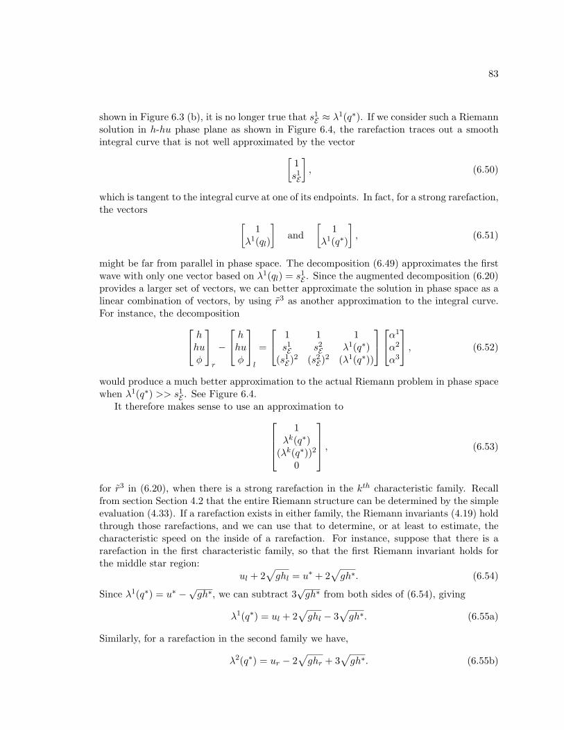
83

shown in Figure 6.3 (b), it is no longer true that s1E ≈ λ1(q∗). If we consider such a Riemannsolution in h-hu phase plane as shown in Figure 6.4, the rarefaction traces out a smoothintegral curve that is not well approximated by the vector[

1s1E

], (6.50)

which is tangent to the integral curve at one of its endpoints. In fact, for a strong rarefaction,the vectors [

1λ1(ql)

]and

[1

λ1(q∗)

], (6.51)

might be far from parallel in phase space. The decomposition (6.49) approximates the firstwave with only one vector based on λ1(ql) = s1E . Since the augmented decomposition (6.20)provides a larger set of vectors, we can better approximate the solution in phase space as alinear combination of vectors, by using r3 as another approximation to the integral curve.For instance, the decomposition hhu

φ

r

−

hhuφ

l

=

1 1 1s1E s2E λ1(q∗)

(s1E)2 (s2E)

2 (λ1(q∗))

α1

α2

α3

, (6.52)

would produce a much better approximation to the actual Riemann problem in phase spacewhen λ1(q∗) >> s1E . See Figure 6.4.

It therefore makes sense to use an approximation to1

λk(q∗)(λk(q∗))2

0

, (6.53)

for r3 in (6.20), when there is a strong rarefaction in the kth characteristic family. Recallfrom section Section 4.2 that the entire Riemann structure can be determined by the simpleevaluation (4.33). If a rarefaction exists in either family, the Riemann invariants (4.19) holdthrough those rarefactions, and we can use that to determine, or at least to estimate, thecharacteristic speed on the inside of a rarefaction. For instance, suppose that there is ararefaction in the first characteristic family, so that the first Riemann invariant holds forthe middle star region:

ul + 2√ghl = u∗ + 2

√gh∗. (6.54)

Since λ1(q∗) = u∗ −√gh∗, we can subtract 3

√gh∗ from both sides of (6.54), giving

λ1(q∗) = ul + 2√ghl − 3

√gh∗. (6.55a)

Similarly, for a rarefaction in the second family we have,

λ2(q∗) = ur − 2√ghr + 3

√gh∗. (6.55b)

84

Moreover, the differences

λ1(q∗)− λ1(ql) = 3(√

ghl −√gh∗), (6.56a)

λ2(qr)− λ2(q∗) = 3(√

ghr −√gh∗), (6.56b)

indicate the strength of the rarefaction in the first and second field respectively. If we havean estimate h∗, denoted h∗0, then we can estimate (6.55) and (6.56). Recall that in the caseof two rarefactions, the middle state depth could be exactly determined, and h∗0 = h∗. Ifonly one rarefaction exists, considering Theorem 4.2 and (4.33), a single secant iterationprovides an estimate h∗0 ≥ h∗. This provides a conservative estimate for (6.55a) or (6.55b),and for the strength of the single rarefaction.

6.7.3 Choosing the Vector r3

Allowing various forms for the eigenvector r3 presents an additional task when developingalgorithms for an approximate Riemann solver, however, it also endows the Riemann solver(6.20) with flexibility that will allow it to accommodate diverse types of Riemann prob-lems. The choice can be systematically made, based on some practical considerations andobservations.

First, note that in the augmented Riemann solver (6.20), when using a vector of theform

r3 =[1 s (s)2 0

]T, (6.57)

where s is the speed of the wave, the effective depths defined by the second componentof the decomposition are equivalent to the actual depths defined by the first component.Therefore, positivity of the effective depths can be easily checked after the decomposition.If any are negative, the decomposition can be re-performed with (6.45) for r3, ensuringpositivity. In practice this may only be necessary for Riemann problems near a potentialdry state.

For problems where there is no strong rarefaction, the vectors in (6.51) might becomenearly co-linear, and (6.52) might become poorly conditioned, suggesting that (6.45) is abetter choice for r3. For problems with two large rarefactions, positivity can be an issuedue to incipient cavitation—described in Section 4.3—and so (6.45) might again be theappropriate choice. As one last caveat, it is possible to have a very large rarefaction whereλ1(q∗0) approaches s2E , or similarly for λ2(q∗0), however, this possibility is reduced by theestimate h∗0 ≥ h∗, since the inequality produces conservative estimates for the speeds (6.55).Therefore, if this occurs, it must be due to inadequate estimations of s1E or s2E in the case ofa shock. This problem is pronounced in regions of vanishing depths, and will be discussedin detail in the next section where a unified solution will produce a robust solver for thevarious types of Riemann problems.

To conclude this section, note that when a vector of the form (6.57) is used in the aug-mented Riemann solver for r3, using the first two components of the decomposition and thespeeds to define waves for the update is entirely equivalent to using the flux decomposition.The approximate Riemann solution must conserve the first two components of the solutionthen, even when the Roe speeds are not used. A decomposition of this form therefore unifies

85

the f -wave approach and the standard approximate Riemann solvers, by introducing an-other wave. If maintaining this property is desired, even when linear dependence preventsusing an approximation to (6.53), the vector[

1 sE (sE)2 0]T, (6.58)

where sE = 12(s1E + s2E), provides an alternative that avoids linear dependence. This is also

a suitable solution to the necessary fix required if r3 is associated with a zero speed sE .

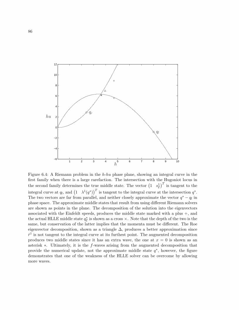
86

1 2 3 4 5 6 7 8 9 10−6

−4

−2

0

2

4

6

8

10

12

hu

h

qr

ql

Figure 6.4: A Riemann problem in the h-hu phase plane, showing an integral curve in thefirst family when there is a large rarefaction. The intersection with the Hugoniot locus inthe second family determines the true middle state. The vector

(1 s1E

)T is tangent to the

integral curve at ql, and(1 λ1(q∗)

)T is tangent to the integral curve at the intersection q∗.The two vectors are far from parallel, and neither closely approximate the vector q∗ − ql inphase space. The approximate middle states that result from using different Riemann solversare shown as points in the plane. The decomposition of the solution into the eigenvectorsassociated with the Einfeldt speeds, produces the middle state marked with a plus +, andthe actual HLLE middle state q∗E is shown as a cross ×. Note that the depth of the two is thesame, but conservation of the latter implies that the momenta must be different. The Roeeigenvector decomposition, shown as a triangle ∆, produces a better approximation sincer1 is not tangent to the integral curve at its furthest point. The augmented decompositionproduces two middle states since it has an extra wave, the one at x = 0 is shown as anasterisk ∗. Ultimately, it is the f -waves arising from the augmented decomposition thatprovide the numerical update, not the approximate middle state q∗, however, the figuredemonstrates that one of the weakness of the HLLE solver can be overcome by allowingmore waves.

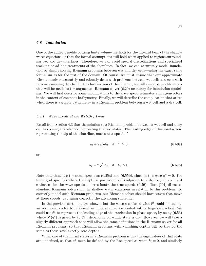
87

6.8 Inundation

One of the added benefits of using finite volume methods for the integral form of the shallowwater equations, is that the formal assumptions still hold when applied to regions surround-ing wet and dry interfaces. Therefore, we can avoid special discretizations and specializedtracking or ad hoc treatments of the shorelines. In fact, we can accurately model inunda-tion by simply solving Riemann problems between wet and dry cells—using the exact sameformalism as for the rest of the domain. Of course, we must ensure that our approximateRiemann solver accurately and robustly deals with problems between wet cells and cells withzero or vanishing depths. In this last section of the chapter, we will describe modificationsthat will be made to the augmented Riemann solver (6.20) necessary for inundation model-ing. We will first describe some modifications to the wave speed estimates and eigenvectorsin the context of constant bathymetry. Finally, we will describe the complication that ariseswhen there is variable bathymetry in a Riemann problem between a wet cell and a dry cell.

6.8.1 Wave Speeds at the Wet-Dry Front

Recall from Section 4.3 that the solution to a Riemann problem between a wet cell and a drycell has a single rarefaction connecting the two states. The leading edge of this rarefaction,representing the tip of the shoreline, moves at a speed of

ul + 2√ghl if hl > 0, (6.59a)

or

ur − 2√ghr if hr > 0. (6.59b)

Note that these are the same speeds as (6.55a) and (6.55b), since in this case h∗ = 0. Forfinite grid spacings where the depth is positive in cells adjacent to a dry region, standardestimates for the wave speeds underestimate the true speeds (6.59). Toro [101] discussesstandard Riemann solvers for the shallow water equations in relation to this problem. Tocorrectly model such Riemann problems, our Riemann solver should have waves that moveat these speeds, capturing correctly the advancing shoreline.

In the previous section it was shown that the wave associated with r3 could be used asan additional vector to represent an integral curve associated with a large rarefaction. Wecould use r3 to represent the leading edge of the rarefaction in phase space, by using (6.53)where λk(q∗) is given by (6.59), depending on which state is dry. However, we will take aslightly different approach that will allow the same definitions in the Riemann solver for allRiemann problems, so that Riemann problems with vanishing depths will be treated thesame as those with exactly zero depths.

When one of the initial states in a Riemann problem is dry the eigenvalues of that stateare undefined, so that s1E must be defined by the Roe speed λ1 when hl = 0, and similarly

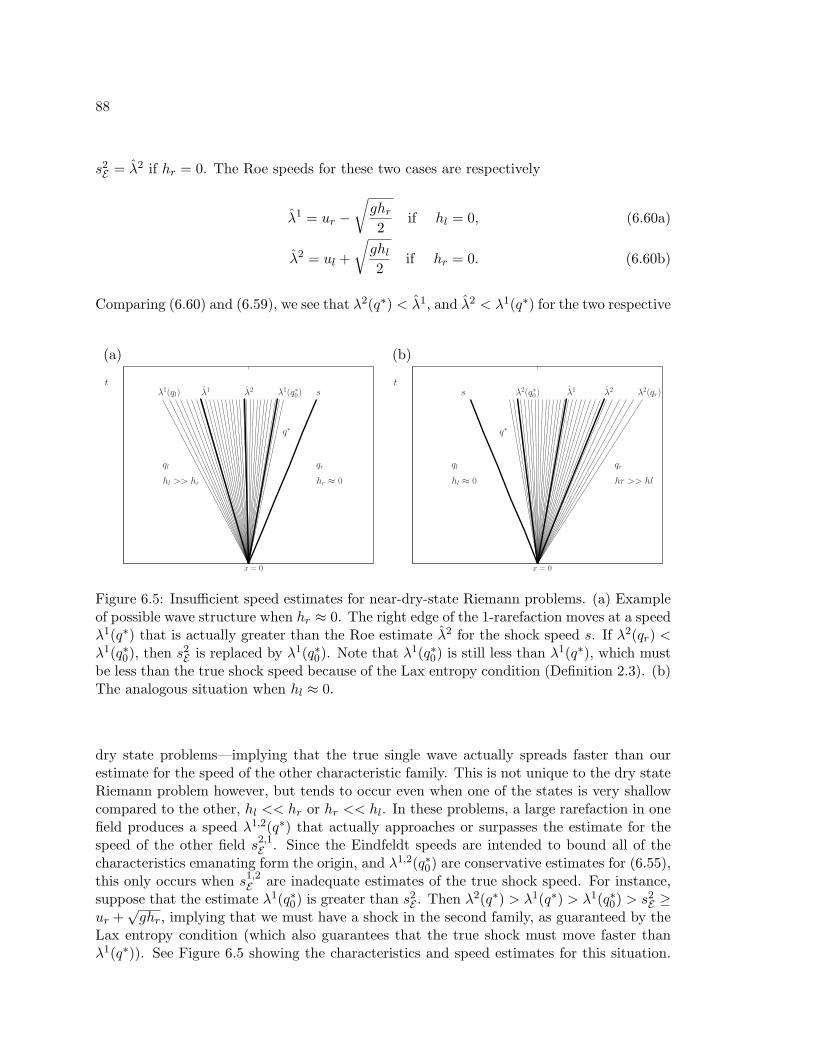
88

s2E = λ2 if hr = 0. The Roe speeds for these two cases are respectively

λ1 = ur −√ghr2

if hl = 0, (6.60a)

λ2 = ul +

√ghl2

if hr = 0. (6.60b)

Comparing (6.60) and (6.59), we see that λ2(q∗) < λ1, and λ2 < λ1(q∗) for the two respective

(a) (b)

ql

hl >> hr

qr

hr ≈ 0

sλ1(ql) λ1 λ2 λ1(q∗0)

q∗

x = 0

t

ql

hl ≈ 0

qr

hr >> hl

s λ2(q∗0) λ1 λ2 λ2(qr)

q∗

x = 0

t

Figure 6.5: Insufficient speed estimates for near-dry-state Riemann problems. (a) Exampleof possible wave structure when hr ≈ 0. The right edge of the 1-rarefaction moves at a speedλ1(q∗) that is actually greater than the Roe estimate λ2 for the shock speed s. If λ2(qr) <λ1(q∗0), then s2E is replaced by λ1(q∗0). Note that λ1(q∗0) is still less than λ1(q∗), which mustbe less than the true shock speed because of the Lax entropy condition (Definition 2.3). (b)The analogous situation when hl ≈ 0.

dry state problems—implying that the true single wave actually spreads faster than ourestimate for the speed of the other characteristic family. This is not unique to the dry stateRiemann problem however, but tends to occur even when one of the states is very shallowcompared to the other, hl << hr or hr << hl. In these problems, a large rarefaction in onefield produces a speed λ1,2(q∗) that actually approaches or surpasses the estimate for thespeed of the other field s2,1E . Since the Eindfeldt speeds are intended to bound all of thecharacteristics emanating form the origin, and λ1,2(q∗0) are conservative estimates for (6.55),this only occurs when s1,2E are inadequate estimates of the true shock speed. For instance,suppose that the estimate λ1(q∗0) is greater than s2E . Then λ2(q∗) > λ1(q∗) > λ1(q∗0) > s2E ≥ur +

√ghr, implying that we must have a shock in the second family, as guaranteed by the

Lax entropy condition (which also guarantees that the true shock must move faster thanλ1(q∗)). See Figure 6.5 showing the characteristics and speed estimates for this situation.

89

It therefore makes sense to redefine the speeds s1E and s2E in the augmented solver (6.20),

sE1 = min(s1E , λ

2(q∗0)), (6.61a)

sE2 = max(s2E , λ

1(q∗0)), (6.61b)

whenever there is a rarefaction in the first or second characteristic field respectively. Notethat when there is a rarefaction, because h∗0 ≥ h∗, the new definition (6.61) only decreasesthe Einfeldt speed s1E to a value still greater than the true speed of the 1-shock, and onlyincreases s2E to a value still less than the true speed of the 2-shock.

Note that with the expanded definition (6.61), when we have a dry state problem, theintegral curve is now approximated with r1 and r2, and the speeds of the waves associatedwith these vectors are the same as the far edges of the rarefaction, including the advancing(or receding) wet/dry front. For these problems, the vector r3 should be defined by (6.45),which ensures positivity since the HLLE depth h∗E is determined using the speeds (6.61).(See the comment after Theorem 3.1.)

It should be noted that for the practical issue of implementing the corrections describedin this section, dry state problems need no special consideration. For instance, if a rarefac-tion exists in either family, say the first family, then the value h∗ is quickly estimated andthe speed of the rarefaction edge (6.55a) estimated. This determines the speed sE

2, whichtypically is the same as s2E . If λ1(q∗0) is sufficiently close to either s1E (as in the case of aweak rarefaction) or s2E (such as for a near dry state problem), then r3 is defined by (6.45),and the associated wave moves at a speed sE = 1

2(s1E + s2E). If two strong rarefactions exist,then r3 is also defined by (6.45) in order to ensure positivity. Otherwise, r3 can be definedby

r3 =[1 λ1(q∗0) (λ1(q∗0))

2 0]T. (6.62)

It is also easy to show that defining ul = 0, when hl = 0, so that λ1(ql) = 0, will have noeffect on the numerical solution, if the above procedure for the wave speeds with a dry stateare taken.

6.8.2 Variable Bathymetry and Shorelines

As with most other approximate Riemann solvers, our wave speed estimates and approx-imate eigenvectors will not be altered by the existence of variable bathymetry and theresulting source term. However, we must treat the Riemann problem between a dry celland a wet cell carefully when there is a jump in bathymetry between the two cells. For in-stance, suppose we are solving the Riemann problem depicted in Figure 6.6, where hr = 0,and hl + bl < br. This situation arises naturally with any discretization near the shoreline(unless special care is taken to ensure that hl + bl = br). Solving such a Riemann problemwith the methods described so far will be shown to produce a spurious result. This is mosteasily seen by considering the steady state problem, where we expect the Riemann solutionto produce no waves, so that the shoreline remains unaffected. However, consider the initial

90

x = 0

bl

hl

6

?

br

hr = 0

Figure 6.6: A Riemann problem at the shoreline, showing hl + bl < br. If this Riemannproblem represents the steady state where ul = 0, solving it without modification will resultin spurious waves from the shoreline.

jump hhuφb

r

−

hhuφb

l

=

−hl0

−g2h

2l

br − bl

. (6.63)

If the steady state is to be maintained with no propagating waves, then (6.63) should be amultiple of the steady state vector r4, which, if we consider the averages of the initial leftand right states, is

−10

−g2hl1

. (6.64)

Preservation of the steady state would therefore require hl = br − bl, which would occur ifthe surface on the left was equal to the dry elevation on the right, which is not the casefor this problem. This makes intuitive sense if one considers the problem from a physicalstandpoint—if the water is motionless, the elevation of the dry topography on the right isirrelevant if it is higher than hl+bl. If we solved the problem as is, spurious waves would begenerated at the shoreline, which is clearly unacceptable. These waves can be quite largein fact for tsunami modeling, where a large domain requires large cells, so that often cellswith depths approaching hundreds of meters or more are adjacent to dry cells.

An easy solution for this steady state problem would be to simply reduce the value brto hl + bl. However, consider what would happen if a small positive velocity was added to

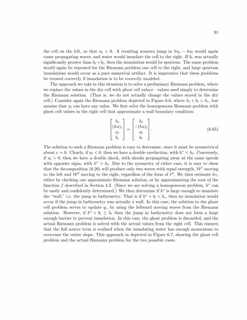
91

the cell on the left, so that ul > 0. A resulting nonzero jump in hur − hul would againcause propagating waves, and water would inundate the cell to the right. If br was actuallysignificantly greater than hl+bl, then the inundation would be spurious. The same problemwould again be repeated for the Riemann problem one cell to the right, and large spuriousinundations would occur as a pure numerical artifact. It is imperative that these problemsbe treated correctly if inundation is to be correctly modeled.

The approach we take in this situation is to solve a preliminary Riemann problem, wherewe replace the values in the dry cell with ghost cell values—values used simply to determinethe Riemann solution. (That is, we do not actually change the values stored in the drycell.) Consider again the Riemann problem depicted in Figure 6.6, where hl + bl > hr, butassume that ul can have any value. We first solve the homogeneous Riemann problem withghost cell values in the right cell that approximate a wall boundary condition:

hr(hu)rφrbr

=

hl

−(hu)lφlbl

. (6.65)

The solution to such a Riemann problem is easy to determine, since it must be symmetricalabout x = 0. Clearly, if ul < 0, then we have a double rarefaction, with h∗ < hl. Conversely,if ul > 0, then we have a double shock, with shocks propagating away at the same speedswith opposite signs, with h∗ > hl. Due to the symmetry of either case, it is easy to showthat the decomposition (6.20) will produce only two waves with equal strength, W1 movingto the left and W2 moving to the right, regardless of the form of r3. We then estimate h∗,either by checking our approximate Riemann solution, or by approximating the root of thefunction f described in Section 4.2. (Since we are solving a homogeneous problem, h∗ canbe easily and confidently determined.) We then determine if h∗ is large enough to inundatethe “wall,” i.e. the jump in bathymetry. That is if h∗ + bl < br, then no inundation wouldoccur if the jump in bathymetry was actually a wall. In this case, the solution to the ghostcell problem serves to update ql, by using the leftward moving waves from the Riemannsolution. However, if h∗ + bl ≥ br then the jump in bathymetry does not form a largeenough barrier to prevent inundation. In this case, the ghost problem is discarded, and theactual Riemann problem is solved with the actual values from the right cell. This ensuresthat the full source term is realized when the inundating water has enough momentum toovercome the entire slope. This approach in depicted in Figure 6.7, showing the ghost cellproblem and the actual Riemann problem for the two possible cases.

92

(a) (b)

(c) (d)

Figure 6.7: The wall boundary condition Riemann problem as a test for the source term.The left panel shows the ghost cell Riemann problems for two different cases, and the rightpanel shows the update for the actual Riemann problem in the same cases. (a) The ghostcell problem has equal and opposite velocities in each cell, with ul > 0, resulting in twoshocks propagating away from the initial interface. The resulting middle depth h∗ is nothigh enough to overtop the jump in bathymetry, h∗ < br − bl. (b) The actual Riemannproblem corresponding to (a). The leftward moving waves from the ghost cell problem getused to update the solution in the left cell. (c) A ghost cell problem similar to that shownin (a), yet with greater initial velocities, causing h∗ > br − bl. (d) The actual Riemannproblem gets used to update the solution in both cells.

93

6.9 Extension to the Two-Dimensional Problem

Recall from Chapter 3 that we extend the basic wave propagation algorithms to multipledimensions by solving normal one-dimensional Riemann problems corresponding to thehigher-dimensional system. For the shallow water equations in two dimensions, recall fromSection 2.5 that the Riemann problem is unchanged, except for an additional wave carryingthe jump in the transverse velocity (vr − vl), moving at the speed u∗. For an f -wave typeof approach, where the transverse flux huv is decomposed into a set of waves, the two-dimensional Riemann problem is solved exactly as the one-dimensional problem, exceptthat the waves defined in the one-dimensional problem have another component carryingthe corresponding jumps in huv, and one additional wave carrying the remaining jump inhuv, moving at an estimate to the speed u∗. For the augmented solver, the jump in huvacross the wave Zp (defined by the one-dimensional problem) is simply vl(Zp)2 if sp < u∗0,and vr(Zp)2 if sp > u∗0, where u∗0 is an estimate to the middle state velocity. The remainingjump

(huv)r − (huv)l −∑

p:sp<u∗0vl(Zp)2 −

∑p:sp>u∗0

vr(Zp)2, (6.66)

then determines the additional f -wave moving at the speed u∗0. Therefore, the only sig-nificant added task for the two-dimensional Riemann problem is to determine an estimateu∗0. It is desired that this average have several properties. First, it should be a simpleand consistent estimate for u∗. Second, in the case of a strong rarefaction such as in theinitial dry state problem, the speed should not be intermediate to the speeds at the edgesof the rarefaction wave. This is because the transverse contact discontinuity in such a caseis to one side of the rarefaction. In fact, for the initial dry state problem, the transversecontact discontinuity is precisely at the advancing wet-dry front moving at the speed of theadvancing edge of the single rarefaction. These properties are satisfied by using the value

u∗0 = min(λ2(q∗0),max(λ1(q∗0)), sE), (6.67)

when a rarefaction exists, and u∗0 = sE otherwise, where sE = 12(s1E+s2E) using the definitions

(6.61). Note that when there is no strong rarefaction, this corresponds to the speed of thewave associated with r3. For a dry state Riemann problem, it corresponds to the speed ofthe advancing front.

94

Chapter 7

ADAPTIVE MESH REFINEMENT FOR TSUNAMI MODELING

So far our efforts have been directed at the difficulty of diverse flow regimes associatedwith tsunamis—our aim has been to develop algorithms that are reasonably robust andaccurate for all of the regimes. Recall that these diverse regimes occur at extremely diversescales, and we have not yet dealt with the obvious difficulty of simply being able to resolvethese diverse scales in a single computation. In this chapter we confront that difficulty bydescribing adaptive mesh refinement algorithms. These algorithms will “bridge the gap”in the sense that they will allow the algorithms described previously to be simultaneouslyapplied to the diverse spatial scales and flow regimes in a single computation. In fact,adaptive mesh refinement is one of the main motivations for designing algorithms that aresuitable for all of the regimes of tsunami flow, otherwise it might be feasible to switchalgorithms for different computations involving different flow regimes.

The initial profile of a tsunami is determined by the geometry and nature of the gen-erating fault motion. For most global scale tsunamis the initial wavelength is hundredsof kilometers, and the disturbance can be spread over thousands of kilometers. (For theSumatra-Andaman earthquake, the rupture zone encompassed a huge swath 400 km wideby 1200 km long—one of the largest single ruptures ever recorded [3, 43]). Since initialamplitudes are often less than a meter, tsunami energy is initially spread thin over largeareas, and this energy does not easily dissipate until it is more locally concentrated. Thisallows tsunamis to travel across entire oceans without significant dissipation. Obviouslymodeling this propagation requires a large computing domain, at least big enough to in-clude the source and coastlines of interest—sometimes in different hemispheres. Fortunatelythe wavelength of this propagation is large enough that we can capture it with a fairly coarsediscretization.

As tsunami waves enter coastal shallow water their wavelength is compressed. Thisoccurs due to the decreasing wave speeds—recall that the wave speeds are u ±

√gh. In

the deep ocean this implies wave speeds of up to 200 m/s, or equivalently 720 km/hr.In the near shore the wave speeds decrease with roughly the square root of depth so thewave is dramatically compressed as the leading edge slows rapidly while the trailing edgeis still in the deep ocean. This compression occurs continually as the waves approach theshore, halving the wavelengths many times over. This energy compression is what tsunamisowe their destructive capacity to—only at the shoreline is the energy dissipated. Thisdecrease in wavelength near the shore requires an equivalent increase in computational gridresolution. If specific features of inundation are to be captured, necessary grid resolutionsmay be several meters—orders of magnitude smaller than in the deep ocean. With theenergy more compressed the flow exhibits more violent and erratic features contributing tothe unpredictability. These flow features add to the need for higher grid refinement.

A simple solution to this problem, and one frequently employed, is to use a set of

95

fixed telescoping grids at the shoreline—typically only near a region or coastline of interest.This is a legitimate approach for many problems, particularly for problems where one ismodeling a single community for future hazard mitigation, and can dedicate days or weeks ofcomputational time to the problem. However, for global-scale modeling this is less than idealfor several reasons. First, it is inefficient when modeling the entire ocean. Although onlya relatively coarse resolution is needed to capture deep ocean propagation, this resolutionis still quite expensive if used throughout an entire ocean for an entire computation. Sincetsunami waves propagate long distances, using fixed grids requires modeling an entire oceanat the level required to resolve the propagating tsunami. This means that a large amountof computing effort gets dedicated to steady-state calculations in regions where nothing ishappening. Second, it requires either under-resolving the majority of coastal regions thatmight be impacted by a global-scale tsunami, or perhaps using some a priori knowledge ofwhere inundation will be the most severe. Since depth and hence wave speeds are a functionof the variable seafloor bathymetry, the compressing energy of a tsunami as it approachesshore is focused by bathymetry in complex and unpredictable ways. Often destruction variesgreatly even along local stretches of coastline. Determining what communities or regions arevulnerable to a given fault event, using fixed grids, essentially requires a separate calculationfor each region. This is certainly not the most efficient use of computational resources, noris it practical for real-time tsunami modeling. Third, the fixed fine-scale grids are typicallyintegrated for the entire computation, even long before the tsunami arrives. This again iscomputationally wasteful and ultimately decreases the degree to which the tsunami can beresolved due to misappropriation of resources.

7.1 Adaptive Mesh Refinement for Hyperbolic Systems

Adaptive refinement methods in general use variable sized grid spacings depending on thenature of the solution in different regions of the domain. The regions of refinement adaptto the changing solution based on some set of criteria relevant to the problem. Thesemethods are particularly attractive for hyperbolic problems since interesting features in thesolutions are often highly localized, yet, because of the wave-like nature of the solutions, thefeatures often move throughout the domain. We have extended Berger-Collela-Oliger [9, 7]adaptive mesh refinement to the problem of tsunami modeling. These methods use multiplelevels of rectangular Cartesian subgrids that use integer refinement ratios in space and time.Multiple subgrids at a given level may exist and are adaptively arranged in patches thatcover important features in the solution (see Figure 7.1). (See Chapter 8 for a discussion ofhow these Cartesian computational grids can be used for more general geometries.) Sincethe size and location of the subgrids can change at any time depending on the level ofrefinement needed in a specific area, the grids can effectively move with important featuresin the solution. These methods were originally developed for hyperbolic systems such asthe Euler equations of compressible gas dynamics, where often shock waves and very steepgradients are highly localized and need much higher levels of refinement than the rest ofdomain. Since the shock waves move throughout the domain, fixed telescoping grids wouldbe ineffective.

These adaptive mesh refinement methods have previously been implemented in the gen-

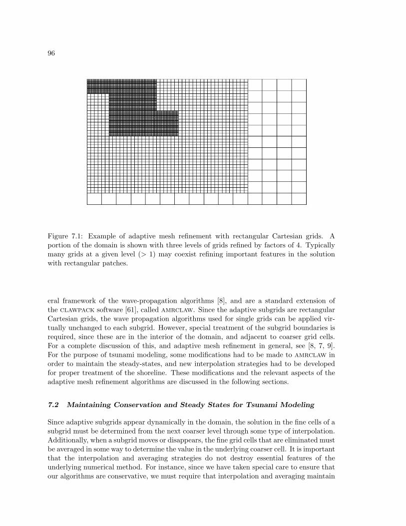
96

Figure 7.1: Example of adaptive mesh refinement with rectangular Cartesian grids. Aportion of the domain is shown with three levels of grids refined by factors of 4. Typicallymany grids at a given level (> 1) may coexist refining important features in the solutionwith rectangular patches.

eral framework of the wave-propagation algorithms [8], and are a standard extension ofthe clawpack software [61], called amrclaw. Since the adaptive subgrids are rectangularCartesian grids, the wave propagation algorithms used for single grids can be applied vir-tually unchanged to each subgrid. However, special treatment of the subgrid boundaries isrequired, since these are in the interior of the domain, and adjacent to coarser grid cells.For a complete discussion of this, and adaptive mesh refinement in general, see [8, 7, 9].For the purpose of tsunami modeling, some modifications had to be made to amrclaw inorder to maintain the steady-states, and new interpolation strategies had to be developedfor proper treatment of the shoreline. These modifications and the relevant aspects of theadaptive mesh refinement algorithms are discussed in the following sections.

7.2 Maintaining Conservation and Steady States for Tsunami Modeling

Since adaptive subgrids appear dynamically in the domain, the solution in the fine cells of asubgrid must be determined from the next coarser level through some type of interpolation.Additionally, when a subgrid moves or disappears, the fine grid cells that are eliminated mustbe averaged in some way to determine the value in the underlying coarser cell. It is importantthat the interpolation and averaging strategies do not destroy essential features of theunderlying numerical method. For instance, since we have taken special care to ensure thatour algorithms are conservative, we must require that interpolation and averaging maintain

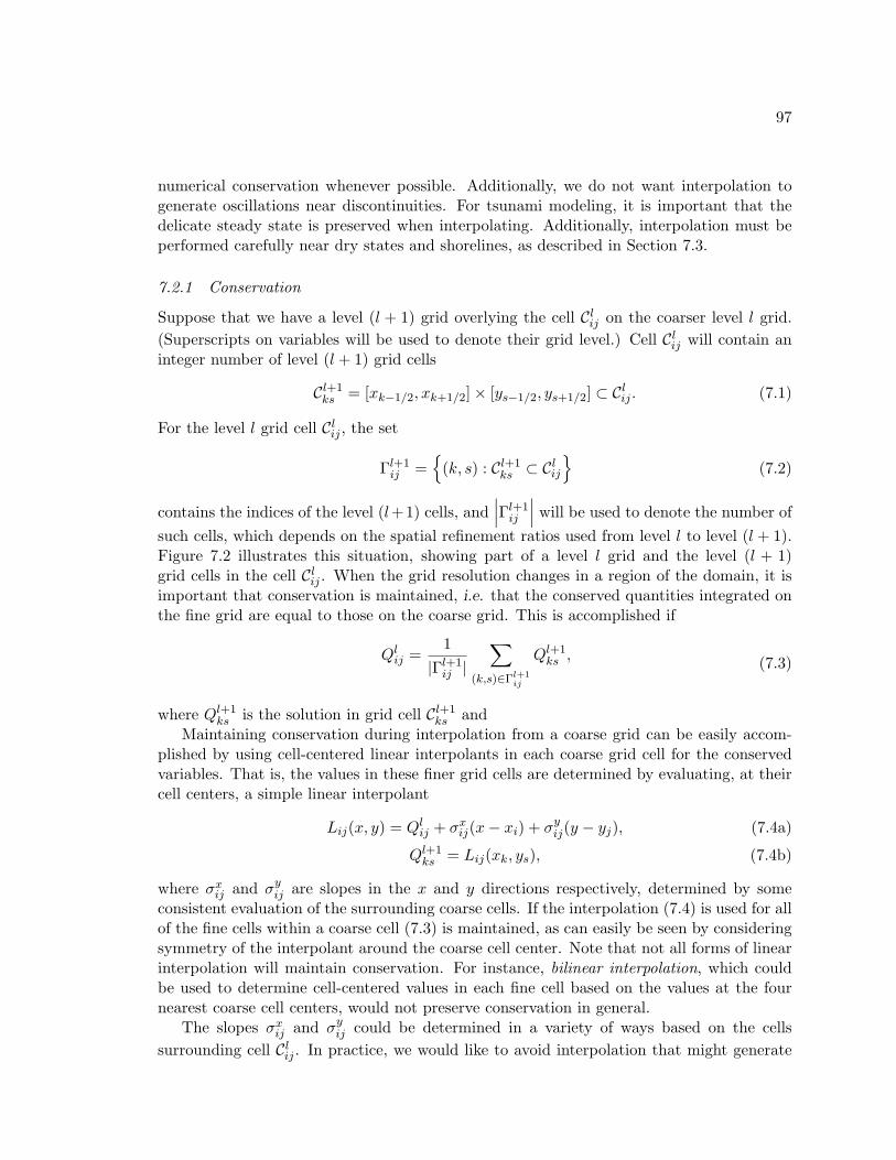
97

numerical conservation whenever possible. Additionally, we do not want interpolation togenerate oscillations near discontinuities. For tsunami modeling, it is important that thedelicate steady state is preserved when interpolating. Additionally, interpolation must beperformed carefully near dry states and shorelines, as described in Section 7.3.

7.2.1 Conservation

Suppose that we have a level (l + 1) grid overlying the cell Clij on the coarser level l grid.(Superscripts on variables will be used to denote their grid level.) Cell Clij will contain aninteger number of level (l + 1) grid cells

Cl+1ks = [xk−1/2, xk+1/2]× [ys−1/2, ys+1/2] ⊂ Clij . (7.1)

For the level l grid cell Clij , the set

Γl+1ij =

(k, s) : Cl+1

ks ⊂ Clij

(7.2)

contains the indices of the level (l+1) cells, and∣∣∣Γl+1ij

∣∣∣ will be used to denote the number ofsuch cells, which depends on the spatial refinement ratios used from level l to level (l + 1).Figure 7.2 illustrates this situation, showing part of a level l grid and the level (l + 1)grid cells in the cell Clij . When the grid resolution changes in a region of the domain, it isimportant that conservation is maintained, i.e. that the conserved quantities integrated onthe fine grid are equal to those on the coarse grid. This is accomplished if

Qlij =1

|Γl+1ij |

∑(k,s)∈Γl+1

ij

Ql+1ks , (7.3)

where Ql+1ks is the solution in grid cell Cl+1

ks andMaintaining conservation during interpolation from a coarse grid can be easily accom-

plished by using cell-centered linear interpolants in each coarse grid cell for the conservedvariables. That is, the values in these finer grid cells are determined by evaluating, at theircell centers, a simple linear interpolant

Lij(x, y) = Qlij + σxij(x− xi) + σyij(y − yj), (7.4a)

Ql+1ks = Lij(xk, ys), (7.4b)

where σxij and σyij are slopes in the x and y directions respectively, determined by someconsistent evaluation of the surrounding coarse cells. If the interpolation (7.4) is used for allof the fine cells within a coarse cell (7.3) is maintained, as can easily be seen by consideringsymmetry of the interpolant around the coarse cell center. Note that not all forms of linearinterpolation will maintain conservation. For instance, bilinear interpolation, which couldbe used to determine cell-centered values in each fine cell based on the values at the fournearest coarse cell centers, would not preserve conservation in general.

The slopes σxij and σyij could be determined in a variety of ways based on the cellssurrounding cell Clij . In practice, we would like to avoid interpolation that might generate

98

Cli−1,j Cli+1,j

Cli,j+1

Cli,j−1

xi−1/2 xi+1/2

yj−1/2

yj+1/2

Cl+1ks

Figure 7.2: Interpolation and averaging between level l and (l+ 1) grids. Using refinementratios of 4 as an example, the 16 level (l + 1) grid cells within a single level l cell Clij areshown. Linear interpolation to determine the fine grid cell values, based on (7.4), preservesconservation as can be seen by considering symmetry. Arithmetic averaging of the fine gridcell values to determine the coarse cell value also preserves conservation.

oscillations near steep gradients in the solution. This could occur if interpolation generatesnew extrema on the fine grid. Recall from Section ??, where we considered the relationshipbetween slope limiters and flux limiters, our goal was to limit the interpolating slopes ingrid cells in order to prevent nonphysical oscillations in the solution by ensuring that newextrema were not generated. We can take the same approach when interpolating from coarseto fine grids—limited slopes can be used for σxij and σyij in order to prevent generating newextrema. For instance, using the minmod slopes

σxij = minmod

(Qli+1,j −Qlij

∆x,Qlij −Qli−1,j

∆x

), (7.5a)

σyij = minmod

(Qli,j+1 −Qlij

∆y,Qlij −Qli,j−1

∆y

), (7.5b)

prevents the generation of new extrema even in two dimensions when using (7.4). Recallthat the minmod function is defined by

minmod(a, b) =

a if |a| < |b| and ab > 0,b if |b| < |a| and ab > 0,0 if ab ≤ 0.

(7.6)

Occasionally, areas of the domain covered by level (l+ 1) grids will no longer need high

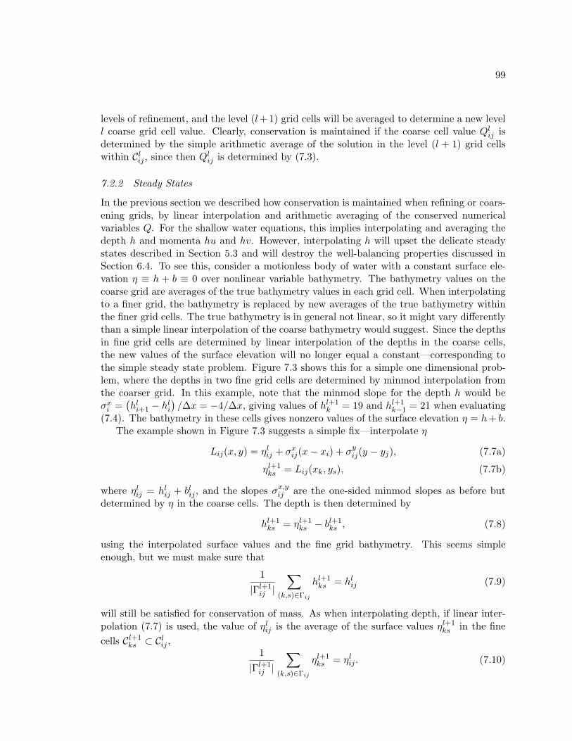
99

levels of refinement, and the level (l+1) grid cells will be averaged to determine a new levell coarse grid cell value. Clearly, conservation is maintained if the coarse cell value Qlij isdetermined by the simple arithmetic average of the solution in the level (l + 1) grid cellswithin Clij , since then Qlij is determined by (7.3).

7.2.2 Steady States

In the previous section we described how conservation is maintained when refining or coars-ening grids, by linear interpolation and arithmetic averaging of the conserved numericalvariables Q. For the shallow water equations, this implies interpolating and averaging thedepth h and momenta hu and hv. However, interpolating h will upset the delicate steadystates described in Section 5.3 and will destroy the well-balancing properties discussed inSection 6.4. To see this, consider a motionless body of water with a constant surface ele-vation η ≡ h + b ≡ 0 over nonlinear variable bathymetry. The bathymetry values on thecoarse grid are averages of the true bathymetry values in each grid cell. When interpolatingto a finer grid, the bathymetry is replaced by new averages of the true bathymetry withinthe finer grid cells. The true bathymetry is in general not linear, so it might vary differentlythan a simple linear interpolation of the coarse bathymetry would suggest. Since the depthsin fine grid cells are determined by linear interpolation of the depths in the coarse cells,the new values of the surface elevation will no longer equal a constant—corresponding tothe simple steady state problem. Figure 7.3 shows this for a simple one dimensional prob-lem, where the depths in two fine grid cells are determined by minmod interpolation fromthe coarser grid. In this example, note that the minmod slope for the depth h would beσxi =

(hli+1 − hli

)/∆x = −4/∆x, giving values of hl+1

k = 19 and hl+1k−1 = 21 when evaluating

(7.4). The bathymetry in these cells gives nonzero values of the surface elevation η = h+ b.The example shown in Figure 7.3 suggests a simple fix—interpolate η

Lij(x, y) = ηlij + σxij(x− xi) + σyij(y − yj), (7.7a)

ηl+1ks = Lij(xk, ys), (7.7b)

where ηlij = hlij + blij , and the slopes σx,yij are the one-sided minmod slopes as before butdetermined by η in the coarse cells. The depth is then determined by

hl+1ks = ηl+1

ks − bl+1ks , (7.8)

using the interpolated surface values and the fine grid bathymetry. This seems simpleenough, but we must make sure that

1|Γl+1ij |

∑(k,s)∈Γij

hl+1ks = hlij (7.9)

will still be satisfied for conservation of mass. As when interpolating depth, if linear inter-polation (7.7) is used, the value of ηlij is the average of the surface values ηl+1

ks in the finecells Cl+1

ks ⊂ Clij ,1

|Γl+1ij |

∑(k,s)∈Γij

ηl+1ks = ηlij . (7.10)

100

Together with (7.8), (7.10) implies

1|Γl+1ij |

∑(k,s)∈Γij

(hl+1ks + bl+1

ks

)= hlij + blij ,

⇒ 1|Γl+1ij |

∑(k,s)∈Γij

hl+1ks = hlij +

blij − 1|Γl+1ij |

∑(k,s)∈Γij

bl+1ks

. (7.11)

We see that if the bathymetry blij in the coarse cell is the average of the bathymetry val-ues bl+1

ks in the fine cells Cl+1ks ⊂ Clij , which is the case if both come from averaging true

bathymetry data, then the terms in parenthesis in (7.11) equal zero and (7.9) is satisfied.We also want to conserve momentum when refining grids. Since the refined depth is

determined by (7.7) and (7.8), it is not necessarily a simple linear function within eachcoarse cell. Following the idea of interpolating η, it might make sense to interpolate thevelocities ul+1

ks and vl+1ks , and then determine the momenta hul+1

ks and hvl+1ks by multiplying

the interpolated velocities by hl+1ks in each fine grid cell. However, this will not conserve

momentum in general, so we will simply interpolate momentum according to (7.4). Thisis not problematic for the most part, since the delicate background steady state that mustbe preserved has zero velocity. However, some precautions must be taken in very shallowregions, where the differences is depth between the interpolated cells are significant relativeto the overall depth. This and other issues that arise in shallow regions and at shorelineswill be explained and treated in the next section.

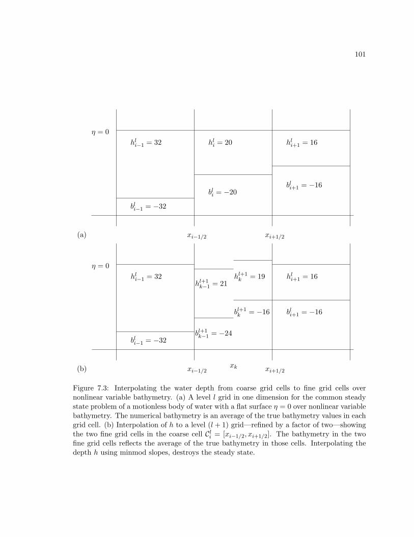
101

(a) xi−1/2 xi+1/2

η = 0

bli−1 = −32

hli−1 = 32

bli = −20

hli = 20

bli+1 = −16

hli+1 = 16

(b)

η = 0

bli−1 = −32

hli−1 = 32

bli+1 = −16

hli+1 = 16

bl+1k−1 = −24

hl+1k−1 = 21

bl+1k = −16

hl+1k = 19

xi−1/2 xi+1/2xk

Figure 7.3: Interpolating the water depth from coarse grid cells to fine grid cells overnonlinear variable bathymetry. (a) A level l grid in one dimension for the common steadystate problem of a motionless body of water with a flat surface η = 0 over nonlinear variablebathymetry. The numerical bathymetry is an average of the true bathymetry values in eachgrid cell. (b) Interpolation of h to a level (l + 1) grid—refined by a factor of two—showingthe two fine grid cells in the coarse cell Cli = [xi−1/2, xi+1/2]. The bathymetry in the twofine grid cells reflects the average of the true bathymetry in those cells. Interpolating thedepth h using minmod slopes, destroys the steady state.

102

7.3 Shorelines and Shallow Regions

7.3.1 Depth

In the previous section it was shown that by interpolating the surface values η to determineh, steady states and conservation can be simultaneously maintained when refining grids.It was assumed that each of the coarse grid cells surrounding Clij had a positive depth,yet, of course, in very shallow shoreline regions it’s possible that some of the coarse cellsare dry. Since the surface elevation is still defined in these cells by η = b, it’s possible tointerpolate as before using (7.7). This is not too problematic if the cell being interpolatedis wet, hlij > 0, and one or more of the surrounding cells are dry, however, it is still lessthan ideal. If hlij = 0 simply interpolating η as before, with ηlij = blij , will cause spuriouswaves to be generated from the shore and must be avoided.

To illustrate this situation, consider again a simple one dimensional example where acoarse grid must be interpolated to determine two fine grid cell values, hl+1

k−1 and hl+1k , in each

coarse cell [xi−1/2, xi+1/2]. Suppose first that hli = 0 and the cell to the left is wet with waterat rest (see Figure 7.4). This reflects the steady state situation that is encountered at theshoreline if no waves are present. When the grid is refined, the bathymetry will be adjustedto values that represent the average of the bathymetry in each fine cell. It is clear by lookingat Figure 7.4 what the surface elevations and depths should be in the two fine grid cells ifthe steady state is to be maintained—the surface elevation should be constant across theinterface xi−1/2, implying that ηl+1

k−1 = 0 or equivalently hl+1k−1 = −bl+1

k−1 = 1, and the depthhl+1k should be zero. (Any other values would generate waves at the interfaces xi−1/2 andxk−1/2, and the steady state would not be maintained.) However, if the surface elevationη was interpolated according to (7.7) using the minmod slope from the left, σxi = 2/∆x,the surface elevations would be ηl+1

k−1 = 1.5 and ηl+1k = 2.5. This would result in depths

hl+1k−1 = −0.5 and hl+1

k = 0.5, which conserves mass, but obviously is not the desired result.At first glance, it might seem that an easy fix to the shoreline situation is to simply

define η = 0 in dry cells, however, a near motionless steady state can exist without beingat sea level η = 0. For instance, when very long waves approach shore the sea level mayrise or fall substantially in certain areas without a pronounced wave. Arriving waves mightthen be viewed as being deviations to this near steady state that is not actually at sealevel. Defining ηli = 0 in a dry cell Cli at the shore, with no regard to the level of waterin Cli−1, could generate spurious waves by introducing a large discontinuity at xi−1/2 uponinterpolation.

A preferable strategy for defining η in dry cells that are being interpolated, is to use thesurrounding wet cells. For example, if hlij = 0, then the surface value ηlij in cell Clij can bedefined by

ηlij =1

|Ωlij |

∑(m,n)∈Ωl

ij

ηli+m,j+n, (7.12)

whereΩlij = (m,n) : m,n ∈ −1, 0, 1, hi+m,j+n > 0 , (7.13)

and |Ωlij | is the number of elements of Ωl

ij—i.e. the number of wet cells in the cells sur-

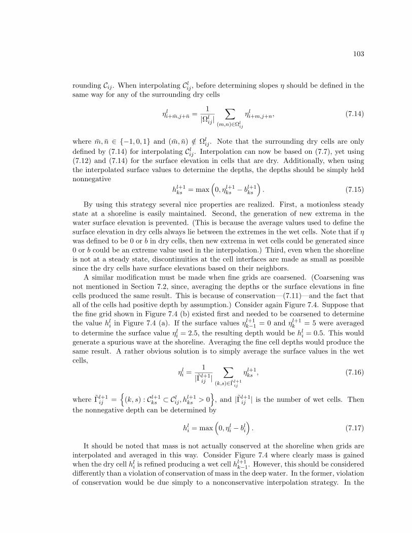
103

rounding Cij . When interpolating Clij , before determining slopes η should be defined in thesame way for any of the surrounding dry cells

ηli+m,j+n =1

|Ωlij |

∑(m,n)∈Ωl

ij

ηli+m,j+n, (7.14)

where m, n ∈ −1, 0, 1 and (m, n) /∈ Ωlij . Note that the surrounding dry cells are only

defined by (7.14) for interpolating Clij . Interpolation can now be based on (7.7), yet using(7.12) and (7.14) for the surface elevation in cells that are dry. Additionally, when usingthe interpolated surface values to determine the depths, the depths should be simply heldnonnegative

hl+1ks = max

(0, ηl+1

ks − bl+1ks

). (7.15)

By using this strategy several nice properties are realized. First, a motionless steadystate at a shoreline is easily maintained. Second, the generation of new extrema in thewater surface elevation is prevented. (This is because the average values used to define thesurface elevation in dry cells always lie between the extremes in the wet cells. Note that if ηwas defined to be 0 or b in dry cells, then new extrema in wet cells could be generated since0 or b could be an extreme value used in the interpolation.) Third, even when the shorelineis not at a steady state, discontinuities at the cell interfaces are made as small as possiblesince the dry cells have surface elevations based on their neighbors.

A similar modification must be made when fine grids are coarsened. (Coarsening wasnot mentioned in Section 7.2, since, averaging the depths or the surface elevations in finecells produced the same result. This is because of conservation—(7.11)—and the fact thatall of the cells had positive depth by assumption.) Consider again Figure 7.4. Suppose thatthe fine grid shown in Figure 7.4 (b) existed first and needed to be coarsened to determinethe value hli in Figure 7.4 (a). If the surface values ηl+1

k−1 = 0 and ηl+1k = 5 were averaged

to determine the surface value ηli = 2.5, the resulting depth would be hli = 0.5. This wouldgenerate a spurious wave at the shoreline. Averaging the fine cell depths would produce thesame result. A rather obvious solution is to simply average the surface values in the wetcells,

ηli =1

|Γl+1ij |

∑(k,s)∈Γl+1

ij

ηl+1ks , (7.16)

where Γl+1ij =

(k, s) : Cl+1

ks ⊂ Clij , hl+1ks > 0

, and |Γl+1

ij | is the number of wet cells. Thenthe nonnegative depth can be determined by

hli = max(0, ηli − bli

). (7.17)

It should be noted that mass is not actually conserved at the shoreline when grids areinterpolated and averaged in this way. Consider Figure 7.4 where clearly mass is gainedwhen the dry cell hli is refined producing a wet cell hl+1

k−1. However, this should be considereddifferently than a violation of conservation of mass in the deep water. In the former, violationof conservation would be due simply to a nonconservative interpolation strategy. In the

104

latter, the violation is due to an actual refinement and more accurate representation of theshoreline. Consider a steady state problem for instance where a flat pool of water lies overvariable bathymetry. Keeping the surface elevation of the water fixed and changing gridresolutions clearly changes the amount of mass present, since the area of the region underwater changes. Figure 7.5 shows the same set of grids from Figure 7.1, being used to coverSumatra. The dry cells over land have been erased showing only the wet cells. In morerefined regions the shoreline is more accurately resolved, but the mass must clearly changeas the shoreline is more accurately resolved. It should be pointed out that for the steadystate problem, repeated interpolation and coarsening of the grid would have no net effecton mass.

7.3.2 Momentum

As might be expected, momentum must be treated carefully as well in shoreline regions. InSection 7.2 we showed that in order to conserve momentum we must interpolate momentumdirectly not velocity. However, in shoreline regions it is possible to end up with vanishingor zero depths in fine cells. If momentum is interpolated independently, this can lead tononphysically large velocities in these cells since velocities are determined by dividing themomentum by the depth. (Note that this problem is independent of the issues described inthe preceding discussion—even in regions that have positive depths in fine and coarse cells,nonlinear bathymetry can lead to vanishing depths independent of linearly interpolatedmomentum leading to unbounded velocities.) This must be avoided since the velocities areused in several formulas including the momentum flux.

Suppose that the coarse cell Clij must be interpolated to determine values for the momen-tum hu in the fine cells Cl+1

ks ⊂ Clij . Recall that the minmod slopes used for interpolation inSection 7.2 were employed to prevent extrema in the fine cells Cl+1

ks ⊂ Clij , from surpassingthe bounds of the neighboring coarse cells. Based on this idea, it is possible to limit velocitywhen interpolating while still actually interpolating momentum. This requires determiningbounds for the (l + 1) velocities when interpolating,

ulij = max(m,n)∈S

(u(i+m,j+n)

), (7.18a)

ulij = min(m,n)∈S

(u(i+m,j+n)

), (7.18b)

where, S = −1, 0, 1 × −1, 0, 1. (By considering the corner cells Cli,j±1 and Ci±1,j thebounds are less restrictive and still prevent new local extrema in u). The momentum canthen be interpolated by (7.4) as always, followed by a check of the new velocities hul+1

ks /hl+1ks

in all of the fine cells Cl+1ks ⊂ Clij . If any of these violate the bounds (7.18), then all of the

fine cell momenta are defined by

hul+1ks = hl+1

ks ulij , ∀(k, s) ∈ Γl+1

ij . (7.19)

The fix (7.19) prevents new extrema in u, while still maintaining conservation if all of the

105

fine cells are wet since,

1|Γl+1ij |

∑(k,s)∈Γl+1

ij

hl+1ks u

lij = ulij

1|Γl+1ij |

∑(k,s)∈Γl+1

ij

hl+1ks = ulijh

lij , (7.20)

where the last equality is due to conservation of mass which occurs when all of the fine cellsare wet and hlij > 0. Therefore, if momentum is gained or lost by employing (7.20), it mustoccur because mass is gained or lost when interpolating based on the procedures discussedin Section 7.3.1, and the momentum change is directly proportional to the mass change

1|Γl+1

ij |

∑(k,s)∈Γl+1

ij

hl+1ks u

lij

huijl=

1|Γl+1

ij |

∑(k,s)∈Γl+1

ij

hl+1ks

hijl. (7.21)

Therefore, if momentum is gained or lost at the shoreline it is due directly to the gain orloss in mass. Trying to conserve momentum when mass is gained or lost at the shorelinewould not be a stable approach.

The problem of unbounded velocities can also occur when coarsening a fine grid if someof the fine grid cells are dry. This occurs because of a loss of mass. Consider again Figure 7.4,assuming now that the shoreline is not at the steady state, but has momentum. Supposethat the fine cells in Figure 7.4 (b) must be averaged to determine huli in the coarse cell inFigure 7.4 (a). Suppose that hulk−1 is nonzero. Then averaging the momenta in the twofine cells would result in a coarse cell momentum of huli = hul+1

k−1/2. Obviously this is aproblem since coarsening the depth based on (7.16) and (7.17) resulted in the value hli = 0.An approach similar to that described above for interpolating momentum can be taken,where the momentum is not conserved but is related to the change in mass. The averagedmomentum is multiplied by the ratio of mass in the fine and coarse cells,

hulij =

hli1

|Γl+1ij |

∑(k,s)∈Γl+1

ij

hl+1ks

1|Γl+1ij |

∑(k,s)∈Γl+1

ij

hul+1ks . (7.22)

This prevents unbounded velocities that occur when the coarsened depth is far less thanthe average depth in the fine cells. Note that the ratio in (7.22) is always 1, unless dry finecells exist.

Obviously the formulas and procedures discussed in this section apply to hv and v aswell as hu and u. It should also be noted that the interpolation and averaging formulaspresented in this section can be applied everywhere on the domain, since they reduce to theformulas in Section 7.2 when away from the shoreline.

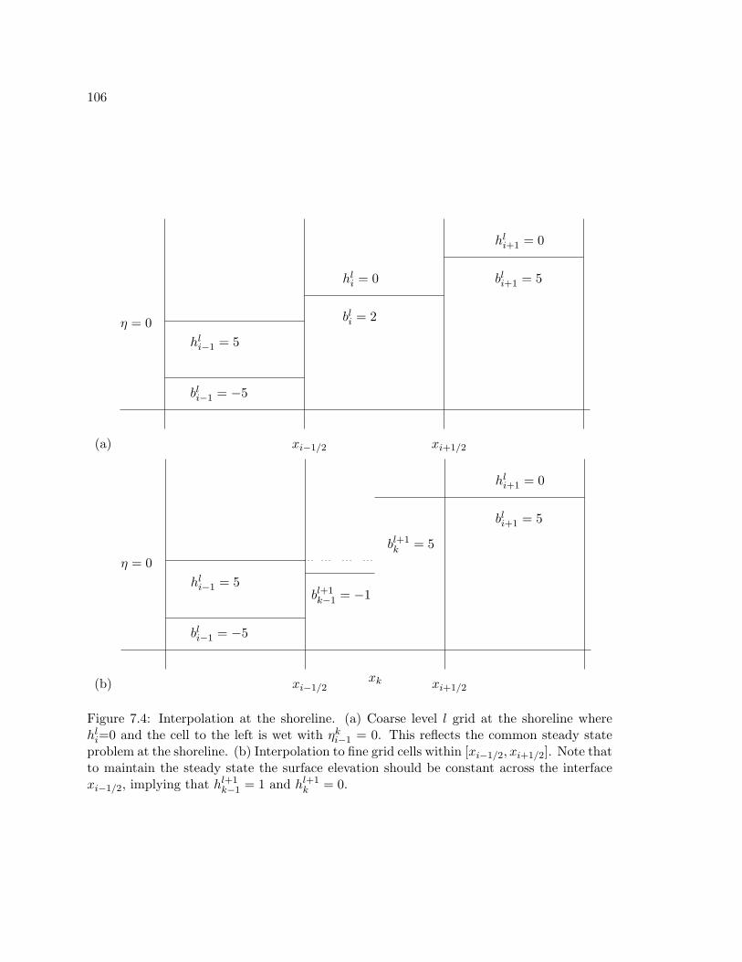
106

(a) xi−1/2 xi+1/2

η = 0

bli−1 = −5

hli−1 = 5

bli = 2

hli = 0 bli+1 = 5

hli+1 = 0

(b) xi−1/2 xi+1/2

η = 0

bli−1 = −5

hli−1 = 5

bli+1 = 5

hli+1 = 0

bl+1k−1 = −1

bl+1k = 5

xk

Figure 7.4: Interpolation at the shoreline. (a) Coarse level l grid at the shoreline wherehli=0 and the cell to the left is wet with ηki−1 = 0. This reflects the common steady stateproblem at the shoreline. (b) Interpolation to fine grid cells within [xi−1/2, xi+1/2]. Note thatto maintain the steady state the surface elevation should be constant across the interfacexi−1/2, implying that hl+1

k−1 = 1 and hl+1k = 0.

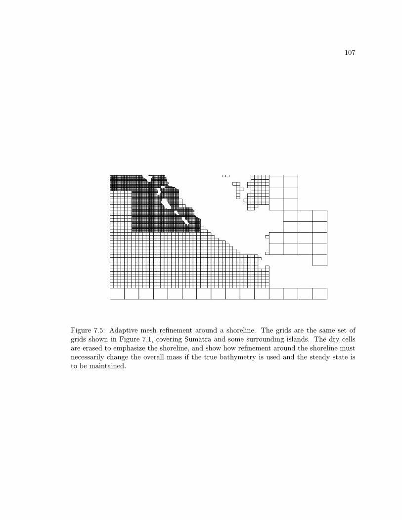
107

Figure 7.5: Adaptive mesh refinement around a shoreline. The grids are the same set ofgrids shown in Figure 7.1, covering Sumatra and some surrounding islands. The dry cellsare erased to emphasize the shoreline, and show how refinement around the shoreline mustnecessarily change the overall mass if the true bathymetry is used and the steady state isto be maintained.

108

7.4 Time Refinement

The adaptive refinement methods discussed in this chapter typically employ refinement intime that is equal to refinement in space. That is, if a coarse level l grid is refined by afactor of n to a finer level (l+ 1) grid, then n timesteps are taken on the fine grid for everytimestep taken on the coarse grid. This is typically required for stability, assuming that thewave speeds on the fine grid and the coarser grids are similar. The CFL condition requiressx∆t < ∆x and sy∆t < ∆y for every grid cell, where sx and sy are the maximum wavespeeds in the x and y directions respectively. If ∆x or ∆y are reduced by a factor of n,then ∆t must be reduced as well. For gas dynamics—the application that these methodswere originally developed for—this is not problematic since typically the wave speeds areas large in areas with the highest refinement—the areas with high pressure and shocks.

With tsunami modeling an interesting peculiarity arises—the wave speeds u ±√gh

decrease with depth, and shallow regions are typically where the most refinement is needed.This means that temporal refinement equal to spatial refinement may be unnecessarilyrestrictive. Suppose that level l grids are restricted to shallow regions to refine inundatingwaves, and the deep ocean is covered by grids of levels 1, · · · , l − 1. If level l grids arerefined by a factor of n in space, timesteps reduced by a factor of n will typically have verysmall Courant numbers since the wave speeds in these shallow regions are much smallerthan on level l − 1 grids and lower. It might be possible to take far fewer timesteps onthese finest grids, speeding the computation considerably. For instance, suppose that levell grids are restricted to regions less than 100 meters deep and refined by a factor of n = 6.A rough calculation (neglecting u) suggests that wave speeds will be faster by a factor of√

4000/100 ≈ 6 on grid levels l− 1 and less, since ocean depths can approach 4000 meters.This implies that timesteps on level l might approach that of time-steps on level l − 1,however, the standard methods would take 6 steps on the level l grids for every step on levell − 1. Of course, wave speeds are also related to water velocity, which can be quite largenear the shoreline, so generally one must be more conservative than this simple calculationsuggests, and we might refine by a factor of 2 at level l

All of the strategies discussed in this chapter have been successfully implemented inthe clawpack and amrclaw routines. We have employed the interpolation and averagingstrategies discussed in Sections 7.2 and 7.3, and we have allowed for anisotropic time re-finement, that allows specifying spatial and temporal refinement separately so that highlyrefined grids restricted to shallow regions can take less restrictive timesteps. These adaptivealgorithms can also be implemented on more complex grids fitted to an idealized surface ofthe earth. The procedure of mapping rectangular Cartesian grids to more general geometriesis discussed in the next chapter.

109

Chapter 8

MODELING TSUNAMIS ON THE EARTH

So far we have assumed that we are solving equations on a flat Cartesian grid in arectangular domain, where the computational space is a direct discrete representation ofthe physical space. Of course, for global-scale tsunami modeling we are interested in solvingthe shallow water equations on the earth, or at least on the surface of an idealized sphere orellipsoid. One approach to such a problem is to recast the shallow water PDEs in sphericalcoordinates, then use latitude and longitude as angular coordinates, however, this entailstransforming derivatives—requiring assumptions about smoothness in the solution that wewish to avoid. It would be preferable to maintain the formalism that we have developedthus far, using the same general form of the equations and simply use a more complex gridthat conforms to the physical domain. The integral conservation law can be applied to anygrid cell and approximated numerically, so the basis of the finite volume approach is stillvalid on grid cells that are more complex than simple rectangles. This approach is generallyapplicable to conservation laws using quite general types of grids on two dimensional curvedmanifolds, and is described in detail in [67, 32, 85]. We will first consider this method on aflat domain, before considering more general curved earth-fitted grids.

8.1 General Quadrilateral Grids on a Flat Surface

We can use the wave propagation algorithm on a more general grid with cells other thanuniform rectangles. We will consider only logically rectangular quadrilateral grids (ie. rect-angular grids with cells in rows and columns that are labeled in a logical manner—cell(i, j) has four neighbors (i± 1, j) and (i, j ± 1)). The simplest implementation of the wavepropagation algorithm on a nonuniform quadrilateral grid, is to use a uniform grid in com-putational space, and then incorporate an appropriate scaling on the numerical update thattakes into account the true physical geometry of each computational cell. We will denotegeneralized coordinates in computational space by ξ and η. Figure 8.1 shows two such gridmappings for illustration. Both quadrilateral grids in physical space are mapped from auniform rectangular grid in computational space shown on top. The grid on the bottom leftis orthogonal whereas the grid on the bottom right is not.

For a finite volume method on a quadrilateral grid, the numerical solution Qij is anapproximation to the average value of the solution in cell (i, j), regardless of the shapeof the cell, and we can base a numerical method on the integral conservation law usinginterface fluxes just as in Chapter 3. Following the notation of LeVeque [67], such a method

110

can be written as

Qn+1ij = Qnij −

∆t|Cij |

(hi+1/2,jFi+1/2,j − hi−1/2,jFi−1/2,j

+hi,j+1/2Gi,j+1/2 − hi,j−1/2Gi,j−1/2

), (8.1)

where

|Cij | = area of cell (i, j),hi±1/2,j = length of side between cells (i± 1, j) and (i, j),hi,j±1/2 = length of side between cells (i, j ± 1) and (i, j),Fi±1/2,j = flux normal to the edge between cells (i, j) and (i± 1, j),

per unit length per unit timeGi,j±1/2 = flux normal to the between cells (i, j) and (i, j ± 1),

per unit length per unit time.

For a uniform Cartesian grid in Euclidean space, the cell area |Cij | is simply the product ofthe edge lengths hi−1/2,j and hi,j−1/2, which are simply the increments of the computationalcoordinates ∆x and ∆y. Additionally the flux Fi−1/2,j is simply the flux in the x direction atthe interface between cells (i−1, j) and (i, j), denoted simply Fi−1/2,j , and similarly Gi,j−1/2

is simply the flux in the y direction at the interface between cells (i, j) and (i, j−1), denotedsimply Gi,j−1/2. The more general numerical method (8.1) then reduces to the standardformula

Qn+1ij = Qnij −

∆t∆x

(Fi+1/2,j − Fi−1/2,j

)− ∆t

∆y(Gi+1/2,j −Gi−1/2,j

), (8.2)

where the computational coordinates are simply x and y. For more general grids, we canwrite (8.1) in terms of computational coordinates following [67], if we set

κij =|Cij |

∆ξ∆η, (8.3a)

Fi−1/2,j =(hi−1/2,j

∆η

)Fi−1/2,j , (8.3b)

Gi,j−1/2 =(hi,j−1/2

∆ξ

)Gi,j−1/2, (8.3c)

so that (8.1) becomes

Qn+1ij = Qnij −

∆tκij∆ξ

(Fi+1/2,j − Fi−1/2,j

)− ∆tκij∆η

(Gi+1/2,j −Gi−1/2,j

). (8.4)

The formulas (8.3) relate the geometry of the computational grid to that of the physicalgrid. The area ratio κij is sometimes called a capacity function since it relates the capacityor true physical area of a grid cell to the area of a cell in computational space. The lengthratios that multiply the normal fluxes are scale factors and will be denoted

γi−1/2,j = hi−1/2,j/∆η (8.5a)

γi,j−1/2 = hi,j−1/2/∆ξ. (8.5b)

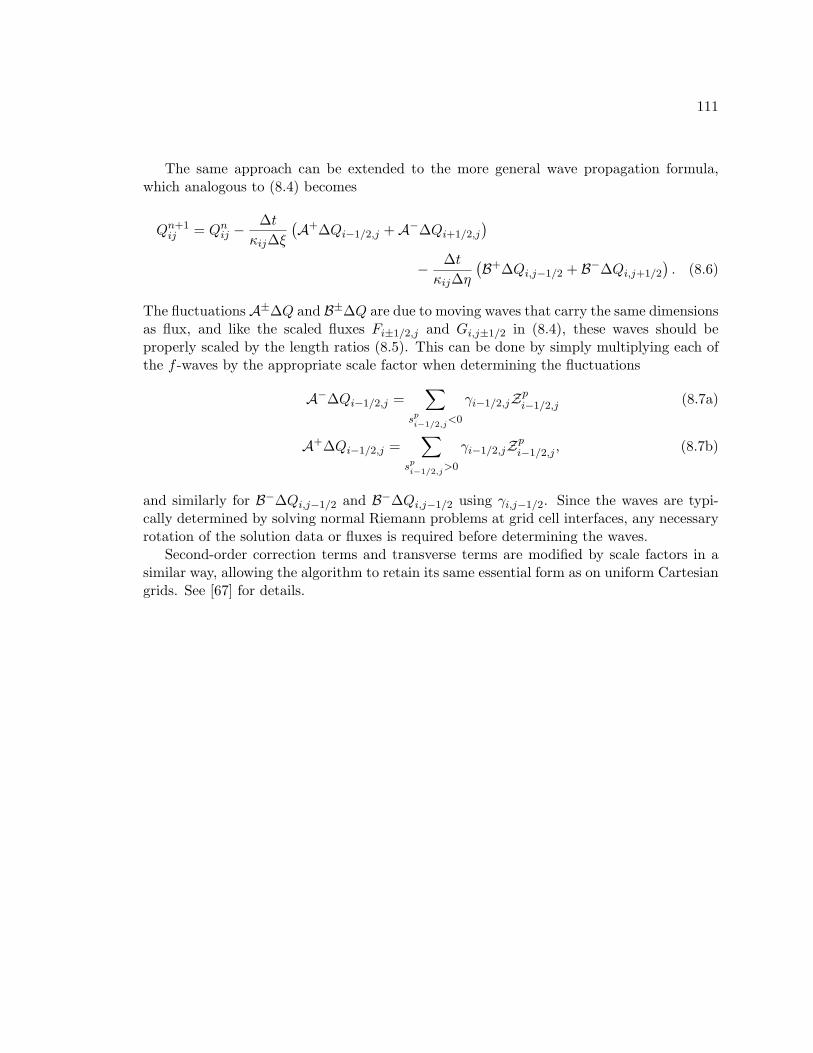
111

The same approach can be extended to the more general wave propagation formula,which analogous to (8.4) becomes

Qn+1ij = Qnij −

∆tκij∆ξ

(A+∆Qi−1/2,j +A−∆Qi+1/2,j

)− ∆tκij∆η

(B+∆Qi,j−1/2 + B−∆Qi,j+1/2

). (8.6)

The fluctuationsA±∆Q and B±∆Q are due to moving waves that carry the same dimensionsas flux, and like the scaled fluxes Fi±1/2,j and Gi,j±1/2 in (8.4), these waves should beproperly scaled by the length ratios (8.5). This can be done by simply multiplying each ofthe f -waves by the appropriate scale factor when determining the fluctuations

A−∆Qi−1/2,j =∑

spi−1/2,j

<0

γi−1/2,jZpi−1/2,j (8.7a)

A+∆Qi−1/2,j =∑

spi−1/2,j

>0

γi−1/2,jZpi−1/2,j , (8.7b)

and similarly for B−∆Qi,j−1/2 and B−∆Qi,j−1/2 using γi,j−1/2. Since the waves are typi-cally determined by solving normal Riemann problems at grid cell interfaces, any necessaryrotation of the solution data or fluxes is required before determining the waves.

Second-order correction terms and transverse terms are modified by scale factors in asimilar way, allowing the algorithm to retain its same essential form as on uniform Cartesiangrids. See [67] for details.

112

(i, j)

-∆ξ

?

6∆η

ξi−1/2 ξi+1/2

ηj−1/2

ηj+1/2

(i, j)?

6

hi−1/2,j

-

hi,j−1/2

CCCCCCCCCCCCCCCCC

hhhhhhhhhhhhhhhhh

(((((((((((((((((

(i, j)

-

hi,j−1/2

CCO

CCWhi−1/2,j

Figure 8.1: Logically rectangular quadrilateral grids. Top: a uniform rectangular grid incomputational space. Bottom Left: a nonuniform orthogonal quadrilateral grid. BottomRight: a nonuniform non-orthogonal quadrilateral grid.

113

8.2 The Shallow Water Equations on Latitude-Longitude Grids

Next we will consider the shallow water equations on the surface of a sphere or moregeneral ellipsoid that approximates the surface of the earth. Recall that the shallow waterequations can be derived by conservation and a hydrostatic assumption, meaning that thepressure gradient balances the gravitational force on a parcel of water at all times in theseflows. Therefore, the equivalent assumption on an ellipsoid is that the gravitational forceis balanced by hydrostatic pressure such that momentum is never in the direction normalto the surface and that pressure depends only on depth. Given the velocity of geophysicalwater flows like tsunamis, and the curvature of the earth, the validity of these assumptionsis unchanged by the curved geometry. For higher velocity shallow flows on a more curvedsurface, where the pressure may depend appreciably on the velocity of the water column, adifferent set of equations may be necessary.

The same basic approach described in Section 8.1 can be used to solve conservation lawson smooth curved manifolds, assuming the conservation law is valid on the manifold. See[85] for a general treatment. For solving the shallow water equations on the surface of anidealized earth, the procedure is simplified from the general procedure for several reasons.First, the surface of an ellipsoid is easily parameterized by latitude and longitude coordi-nates, which means that we can use latitude and longitude to define a uniform quadrilateralgrid in computational space that is logically rectangular. Second, latitude and longitudecoordinates on an ellipsoid define locally orthogonal directions (ie. at any given point on thesurface of the ellipsoid, infinitesimal increases in the two coordinate directions are orthogo-nal in the larger Euclidean space). This allows physical quantities in a grid cell to continueto be represented in a locally orthogonal basis, while simultaneously being aligned with thecomputational grid. This implies that Riemann problems and transverse corrections can beapplied in the standard way without rotation of the data. Lastly, the pole singularity isavoided since the ice-covered poles do not need to be included in the domain. Figure 8.2shows a portion of a uniform computational grid that is mapped to the surface of a referenceellipsoid for the earth.

For the special case of latitude-longitude grids, we will denote the computational coor-dinates by λ for latitude and θ for longitude, and to simplify the formulas we will assumethat λ and θ are in radians. Since the fluxes are everywhere tangent to the ellipsoid surface,the relevant lengths, hi±1/2,j and hi,j±1/2, are the arc lengths of the curved cell edges andthe relevant area of the cell |Cij | is the surface area of a curved surface in physical space. Ifwe consider Euclidean space with the origin at the center of the ellipsoid, and represent thesurface in Euclidean space by the parameterized vector, ~S(θ, λ), the area of the cell (i, j) is

|Cij | =∫ λj+1/2

λj−1/2

∫ θi+1/2

θi−1/2

∣∣∣∣∣∂~S∂θ∣∣∣∣∣∣∣∣∣∣∂~S∂λ

∣∣∣∣∣ dθdλ. (8.8)

Similarly the cell interface lengths are

hi−1/2,j =∫ λj+1/2

λj−1/2

∣∣∣∣∣∂~S∂λ∣∣∣∣∣ dλ, (8.9)

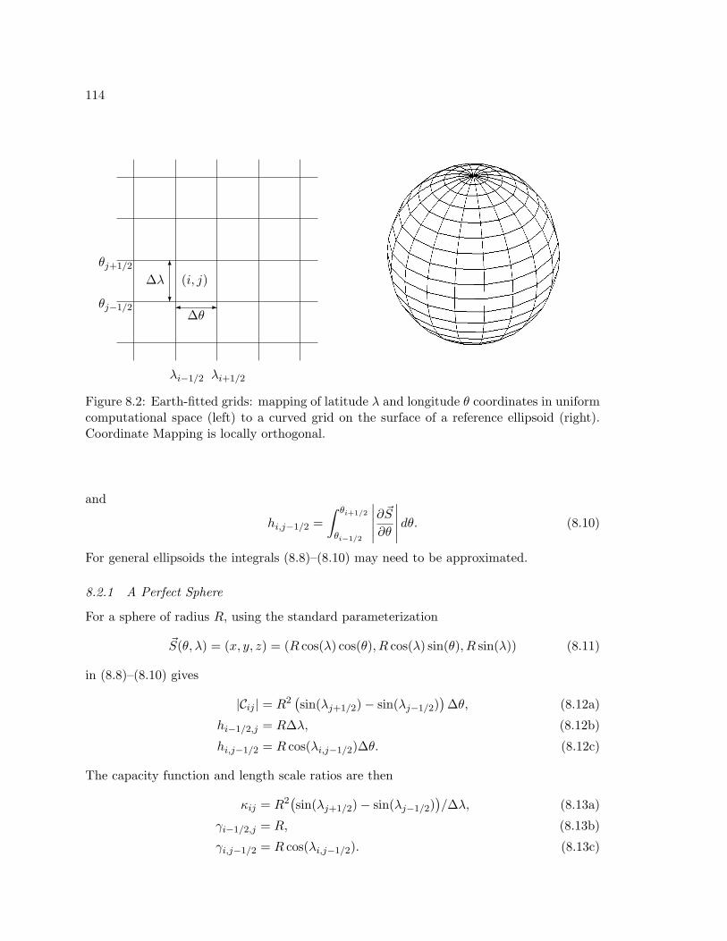
114

(i, j)

-∆θ

?

6∆λ

λi−1/2 λi+1/2

θj−1/2

θj+1/2

Figure 8.2: Earth-fitted grids: mapping of latitude λ and longitude θ coordinates in uniformcomputational space (left) to a curved grid on the surface of a reference ellipsoid (right).Coordinate Mapping is locally orthogonal.

and

hi,j−1/2 =∫ θi+1/2

θi−1/2

∣∣∣∣∣∂~S∂θ∣∣∣∣∣ dθ. (8.10)

For general ellipsoids the integrals (8.8)–(8.10) may need to be approximated.

8.2.1 A Perfect Sphere

For a sphere of radius R, using the standard parameterization

~S(θ, λ) = (x, y, z) = (R cos(λ) cos(θ), R cos(λ) sin(θ), R sin(λ)) (8.11)

in (8.8)–(8.10) gives

|Cij | = R2(sin(λj+1/2)− sin(λj−1/2)

)∆θ, (8.12a)

hi−1/2,j = R∆λ, (8.12b)

hi,j−1/2 = R cos(λi,j−1/2)∆θ. (8.12c)

The capacity function and length scale ratios are then

κij = R2(sin(λj+1/2)− sin(λj−1/2)

)/∆λ, (8.13a)

γi−1/2,j = R, (8.13b)

γi,j−1/2 = R cos(λi,j−1/2). (8.13c)

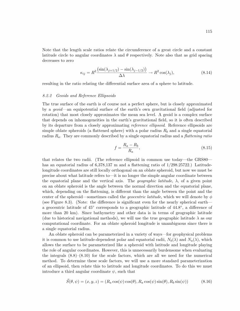
115

Note that the length scale ratios relate the circumference of a great circle and a constantlatitude circle to angular coordinates λ and θ respectively. Note also that as grid spacingdecreases to zero

κij = R2

(sin(λj+1/2)− sin(λj−1/2)

)∆λ

→ R2 cos(λj), (8.14)

resulting in the ratio relating the differential surface area of a sphere to latitude.

8.2.2 Geoids and Reference Ellipsoids

The true surface of the earth is of course not a perfect sphere, but is closely approximatedby a geoid—an equipotential surface of the earth’s own gravitational field (adjusted forrotation) that most closely approximates the mean sea level. A geoid is a complex surfacethat depends on inhomogeneities in the earth’s gravitational field, so it is often describedby its departure from a closely approximating reference ellipsoid. Reference ellipsoids aresimple oblate spheroids (a flattened sphere) with a polar radius Rb and a single equatorialradius Ra. They are commonly described by a single equatorial radius and a flattening ratio

f =Ra −RbRa

, (8.15)

that relates the two radii. (The reference ellipsoid in common use today—the GRS80—has an equatorial radius of 6,378,137 m and a flattening ratio of 1/298.25722.) Latitude-longitude coordinates are still locally orthogonal on an oblate spheroid, but now we must beprecise about what latitude refers to—it is no longer the simple angular coordinate betweenthe equatorial plane and the vertical axis. The geographic latitude, λ, of a given pointon an oblate spheroid is the angle between the normal direction and the equatorial plane,which, depending on the flattening, is different than the angle between the point and thecenter of the spheroid—sometimes called the geocentric latitude, which we will denote by φ(see Figure 8.3). (Note: the difference is significant even for the nearly spherical earth—a geocentric latitude of 45 corresponds to a geographic latitude of 44.8, a difference ofmore than 20 km). Since bathymetry and other data is in terms of geographic latitude(due to historical navigational methods), we will use the true geographic latitude λ as ourcomputational coordinate. For an oblate spheroid longitude is unambiguous since there isa single equatorial radius.

An oblate spheroid can be parameterized in a variety of ways—for geophysical problemsit is common to use latitude-dependent polar and equatorial radii, Nb(λ) and Na(λ), whichallows the surface to be parameterized like a spheroid with latitude and longitude playingthe role of angular coordinates. However, this is unnecessarily burdensome when evaluatingthe integrals (8.8)–(8.10) for the scale factors, which are all we need for the numericalmethod. To determine these scale factors, we will use a more standard parameterizationof an ellipsoid, then relate this to latitude and longitude coordinates. To do this we mustintroduce a third angular coordinate ψ, such that

~S(θ, ψ) = (x, y, z) = (Ra cos(ψ) cos(θ), Ra cos(ψ) sin(θ), Rb sin(ψ)) (8.16)

116

λφ

Ra

Rb

Figure 8.3: Geographic latitude on an oblate ellipse. The cross section of an oblate ellipsewith a single equatorial radius Ra and smaller polar radius Rb is shown. The geographiclatitude λ of a point is the angle between the normal direction and the equatorial plane,not the standard angular coordinate φ.

defines the surface. Note that ψ is neither the geocentric latitude φ nor the geographiclatitude λ, but the three are related by the equation

tan(λ) =1√

1− e2tan(ψ) =

1(1− e2)

tan(φ), (8.17)

where e is the ellipticity defined by

e2 =R2a −R2

b

R2a

. (8.18)

Using (8.16) in the integral (8.8) gives the surface area of a grid cell Cij

|Cij | =∫ ψ(λj+1/2)

ψ(λj−1/2)

∫ θi+1/2

θi−1/2

∣∣∣∣∣∂~S∂θ∣∣∣∣∣∣∣∣∣∣∂~S∂ψ

∣∣∣∣∣ dθdψ= R2

a∆θ∫ ψ(λj+1/2)

ψ(λj−1/2)cos(ψ)

√1− e2 cos2(ψ)dψ

≈ R2a∆θ

∫ ψ(λj+1/2)

ψ(λj−1/2)cos(ψ)

(1− 1

2e2 cos2(ψ)

)dψ

= R2a∆θ

[sin(ψ)

(1− 1

3e2 − 1

6e2 cos2(ψ)

)]ψ=ψ(λj+1/2)

ψ=ψ(λj−1/2)

. (8.19)

Although an exact closed form solution for (8.19) is possible, given the small value of theellipticity of the earth, the O(e4) terms are neglected in the third integral of (8.19), resulting

117

in a less cumbersome formula. Using the implicit definition of ψ(λ) from (8.17) in (8.19)gives

|Cij | =

[∆θR2

a

√1− e2

(sin(λ)√

1− e2 sin2(λ)

)(1− 1

3e2 − 1

6e2 cos2(λ)(

1− e2 sin2(λ)))]λ=λi−1/2

λ=λi−1/2

.

(8.20)Similarly, using (8.16) and (8.17) to determine the length scale factors from (8.9) and (8.10)gives

hi,j−1/2 = ∆θRacos(λi,j−1/2)√

1− e2 sin2(λi,j−1/2)(8.21a)

hi−1/2,j = Ra

∫ ψ(λj+1/2)

ψ(λj−1/2)

√1− e2 cos2(ψ)dψ

≈ Ra

∫ ψ(λj+1/2)

ψ(λj−1/2)

(1− 1

2e2 cos2(ψ)

)dψ

= Ra

[(1− 1

4e2)

arctan(√

1− e2 tan(λ))− 18e2√

1− e2 sin(λ)(1− e2 sin2(2λ)

)]λ=λj+1/2

λ=λj−1/2

. (8.21b)

We can now use (8.20) and (8.21) to determine the capacity function κij and length scaleratios, γi−1/2,j and γi,j−1/2, for (8.6) and (8.7).

Geoid estimates allow an even closer approximation to the true surface of the earth, andcould be incorporated into the surface area of grid cells by using locally scaled radii Ra andRb. However, this would have a negligible effect for tsunami modeling—geoid deviationsfrom the reference ellipsoid are on the order of tens of meters and vary little over hundredsof kilometers. While this is important for applications that require the exact Euclideanposition of a point, such as GPS navigation, it would have little effect on the surface areaand length-scales used to scale computational grid cells.

118

8.3 Coriolis Forces

So far in this chapter we have dealt with effects due entirely to the geometry or curvatureof the earth. In this section we deal with Coriolis forces that are due to the rotation of theearth. Several pseudo-forces arise when Newton’s laws are written with respect to a rotatingcoordinate system. When a particle confined to the surface of the earth changes latitude itsradius of rotation changes so it must accelerate relative to the rotating coordinate system,if its momentum is conserved. This apparent acceleration is due to the Coriolis force. Thispseudo-force can act on a wave as well, if it carries momentum to different latitudes.

The Coriolis acceleration of a particle moving at velocity ~u

∂

∂t~u = −2~ω × ~u, (8.22)

where ~ω is the angular velocity vector of the earth, and the derivative is with respect tothe rotating frame of reference. Since we are solving the shallow water equations on alatitude longitude grid, our momentum variables are conveniently represented in the ro-tating local orthogonal coordinates in the directions of increasing longitude and latitude,not a rotating Euclidean set of axes. If we denote the time dependent unit vectors in thelatitude and longitude directions eλ and eθ respectively, then our momentum vector is~hu ≡ (hu eθ + hv eλ). The rate change in momentum in the rotating coordinate system dueto the Coriolis acceleration (8.22) is then

∂

∂t~hu = −2|ω| (cos(λ) eλ + sin(λ) er)× (hu eθ + hv eλ) ,

= 2|ω| (hv sin(λ) eθ − hu sin(λ) eλ + hu cos(λ) er) . (8.23)

Neglecting the acceleration in the radial direction, (8.23) gives the Coriolis force in thetangent plane

∂

∂t

[huhv

]= 2|ω| sin(λ)

[hv−hu

], (8.24)

where as always the first and second components of the vectors are in the locally orthogonaldirections, denoted by eθ and eλ respectively. Equation (8.24) makes it clear that theCoriolis force is essentially another source term, similar to variable bathymetry and friction.That is, (8.24) can be written

∂

∂tq = ψω, (8.25)

where

ψω = 2|ω| sin(λ)

0hv−hu

. (8.26)

Since there is no relevant steady state due to the Coriolis force, it can be integrated byfractional stepping, discussed in Section 3.6.

119

8.4 Frictional Forces

The shallow water equations are derived for a nonviscous fluid with a uniform velocityprofile in the vertical direction so that there is no boundary layer between the fluid and theunderlying substrate. The validity of this approximation becomes more and more tenuousas the fluid depth decreases and the velocity of the fluid increases. These flow characteristicsare exhibited in the extreme inundation regimes, motivating the use of empirically derivedfriction terms in the shallow water equations when tsunami modeling. These source termsare often based on experimental studies of wave runup given various types of substrates(gravel, sand, concrete etc. e.g. [17]). Friction source terms should therefore be usedcautiously and possibly only for depths below some cutoff value—although they are oftenvery small for regions with any appreciable depth.

The shallow water equations with friction become

∂h

∂t+

∂

∂x(hu) +

∂

∂y(hv) = 0, (8.27a)

∂

∂t(hu) +

∂

∂x(hu2 +

12gh2) +

∂

∂y(huv) = −gh ∂b

∂x− τx, (8.27b)

∂

∂t(hv) +

∂

∂x(huv) +

∂

∂y(12gh2 + hv2) = −gh∂b

∂y− τy, (8.27c)

where

τx =gn2

h7/3hu√

(hu)2 + (hv)2, (8.28)

and

τy =gn2

h7/3hv√

(hu)2 + (hv)2, (8.29)

where n is the Manning coefficient—an empirically determined constant. Typical values forthe Manning coefficient range from n = 0.013 to n = 0.025 depending on the application andthe substrate (e.g. [17]). Since no relevant steady state exists due to friction for tsunamis(the case is very different for river flows), the source term due to friction can be included byfractional stepping. This is the same as for Coriolis forces, discussed in Section 8.3. However,note that an implicit numerical method should be used since the terms can become quitelarge and time-steps are determined by the CFL condition from the underlying hyperbolicpart of the problem.

120

Chapter 9

MISCELLANEOUS NUMERICAL RESULTS

In this chapter several test problems will be shown using the methods described through-out this thesis. In some cases the results will be compared to other modern Godunov-typemethods for the shallow water equations. A description of the other methods is not providedhere, but can be found in the cited references. All of the numerical results using the meth-ods described in this thesis are implemented in TsunamiClaw , described in Appendix A,which is an extension of LeVeque’s clawpack software [61].

9.1 Some One-Dimensional Test Problems

9.1.1 Transcritical Flow with a Shock

This one dimensional test was borrowed from [10], and was originally computed in [37] andlater discussed in [26]. The domain is x ∈ [0, 25], t ∈ [0, 25], with initial data h(x, 0) ≡ 0.33and hu(x, 0) ≡ 0.18. Dirichlet boundary conditions must be imposed with hu(0, t) = 0.18and h(25, t) = 0.33. The bottom topography is given by

b(x) =

0.2− 0.05 (x− 10)2 if 8 < x < 12,0 otherwise.

(9.1)

The goal of the problem is to investigate convergence to a non-stationary steady state.The eventual solution contains a critical point and stationary shock. (Stationary and slowmoving shocks are notorious for generating spurious oscillations, even for shock-capturingschemes [4, 51].) Bouchut computed this problem using several modern numerical schemes,as described in [10]. These solutions are shown in Figure 9.1 (a), which is borrowed directlyfrom [10]. Note that all but one of the methods is free from spurious oscillations. Figure 9.1(b) shows the numerical solution using the augmented Riemann solver and wave propagationmethods developed and described in this thesis. All of the numerical solutions shown werecomputed with 200 points. Figure 9.2 shows a close up of the solution at t = 200 in thecritical region. First and second order versions of the methods described in [10] as well asthe first and second order methods described in this thesis are compared in Figure 9.2.

Figure 9.3 shows the momentum hu for the various schemes for this same test problem.Note that the steady state should have hu constant throughout the domain. Since the shockoccurs in the middle of a grid cell, the numerical solution in the single grid cell overlappingthe shock has a different larger value for hu than what the true solution has. The data inthis grid cell should lie on (or close to) the Hugoniot locus connecting the data to the rightand left of the grid cell. Shock data moving into the grid cell from either side preserve thesteady state in this cell. Therefore, the spike seen at the location of this shock remains evenas the grid is refined and the solution converges.

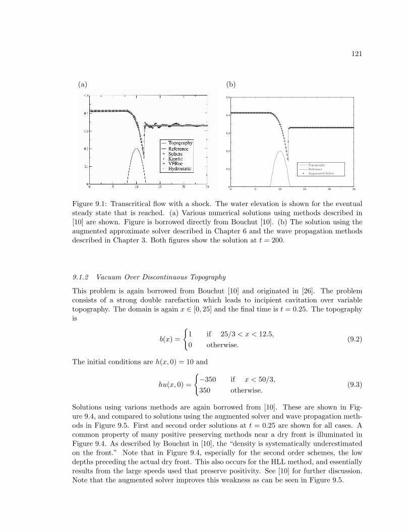
121

(a) (b)

0 5 10 15 20 250

0.1

0.2

0.3

0.4

0.5

Topography

Reference

Augmented Solver

Figure 9.1: Transcritical flow with a shock. The water elevation is shown for the eventualsteady state that is reached. (a) Various numerical solutions using methods described in[10] are shown. Figure is borrowed directly from Bouchut [10]. (b) The solution using theaugmented approximate solver described in Chapter 6 and the wave propagation methodsdescribed in Chapter 3. Both figures show the solution at t = 200.

9.1.2 Vacuum Over Discontinuous Topography

This problem is again borrowed from Bouchut [10] and originated in [26]. The problemconsists of a strong double rarefaction which leads to incipient cavitation over variabletopography. The domain is again x ∈ [0, 25] and the final time is t = 0.25. The topographyis

b(x) =

1 if 25/3 < x < 12.5,0 otherwise.

(9.2)

The initial conditions are h(x, 0) = 10 and

hu(x, 0) =

−350 if x < 50/3,350 otherwise.

(9.3)

Solutions using various methods are again borrowed from [10]. These are shown in Fig-ure 9.4, and compared to solutions using the augmented solver and wave propagation meth-ods in Figure 9.5. First and second order solutions at t = 0.25 are shown for all cases. Acommon property of many positive preserving methods near a dry front is illuminated inFigure 9.4. As described by Bouchut in [10], the “density is systematically underestimatedon the front.” Note that in Figure 9.4, especially for the second order schemes, the lowdepths preceding the actual dry front. This also occurs for the HLL method, and essentiallyresults from the large speeds used that preserve positivity. See [10] for further discussion.Note that the augmented solver improves this weakness as can be seen in Figure 9.5.

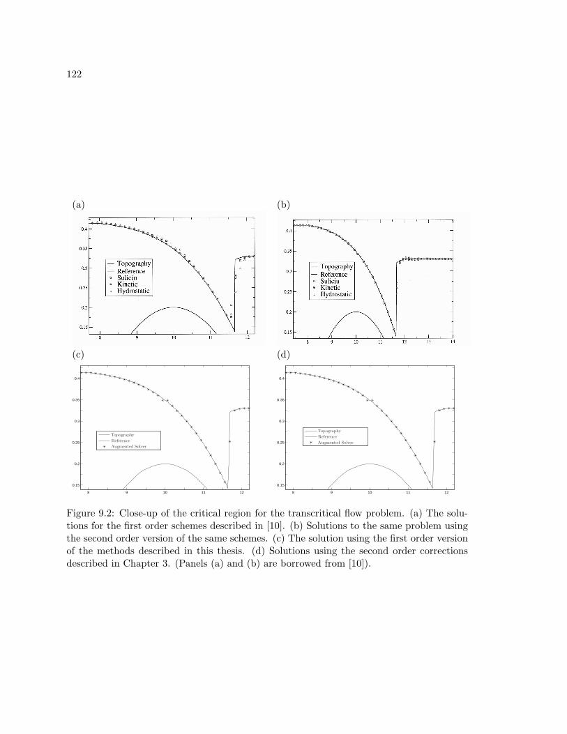
122

(a) (b)

(c) (d)

8 9 10 11 12

0.15

0.2

0.25

0.3

0.35

0.4

Topography

Reference

Augmented Solver

8 9 10 11 12

0.15

0.2

0.25

0.3

0.35

0.4

Topography

Reference

Augmented Solver

Figure 9.2: Close-up of the critical region for the transcritical flow problem. (a) The solu-tions for the first order schemes described in [10]. (b) Solutions to the same problem usingthe second order version of the same schemes. (c) The solution using the first order versionof the methods described in this thesis. (d) Solutions using the second order correctionsdescribed in Chapter 3. (Panels (a) and (b) are borrowed from [10]).

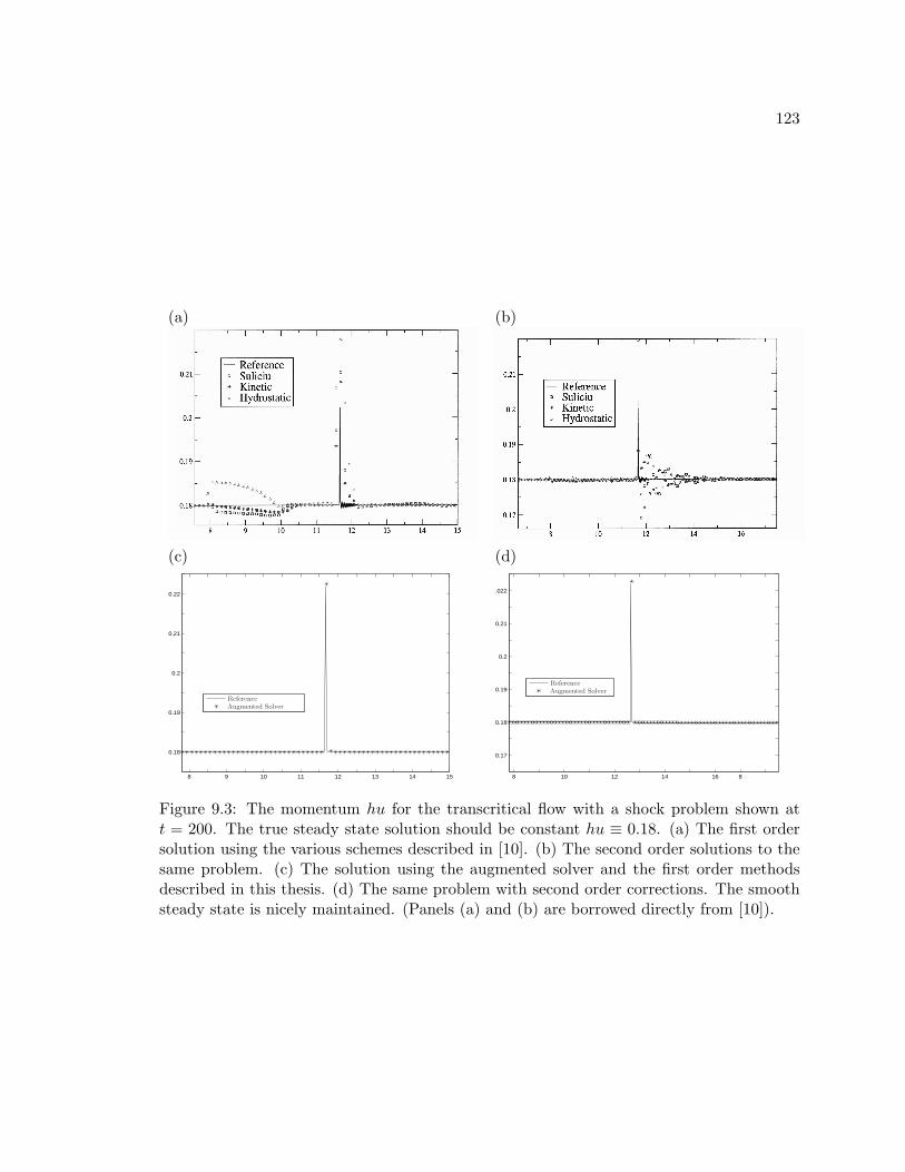
123

(a) (b)

(c) (d)

8 9 10 11 12 13 14 15

0.18

0.19

0.2

0.21

0.22

Reference

Augmented Solver

8 10 12 14 16 8

0.17

0.18

0.19

0.2

0.21

.022

Reference

Augmented Solver

Figure 9.3: The momentum hu for the transcritical flow with a shock problem shown att = 200. The true steady state solution should be constant hu ≡ 0.18. (a) The first ordersolution using the various schemes described in [10]. (b) The second order solutions to thesame problem. (c) The solution using the augmented solver and the first order methodsdescribed in this thesis. (d) The same problem with second order corrections. The smoothsteady state is nicely maintained. (Panels (a) and (b) are borrowed directly from [10]).

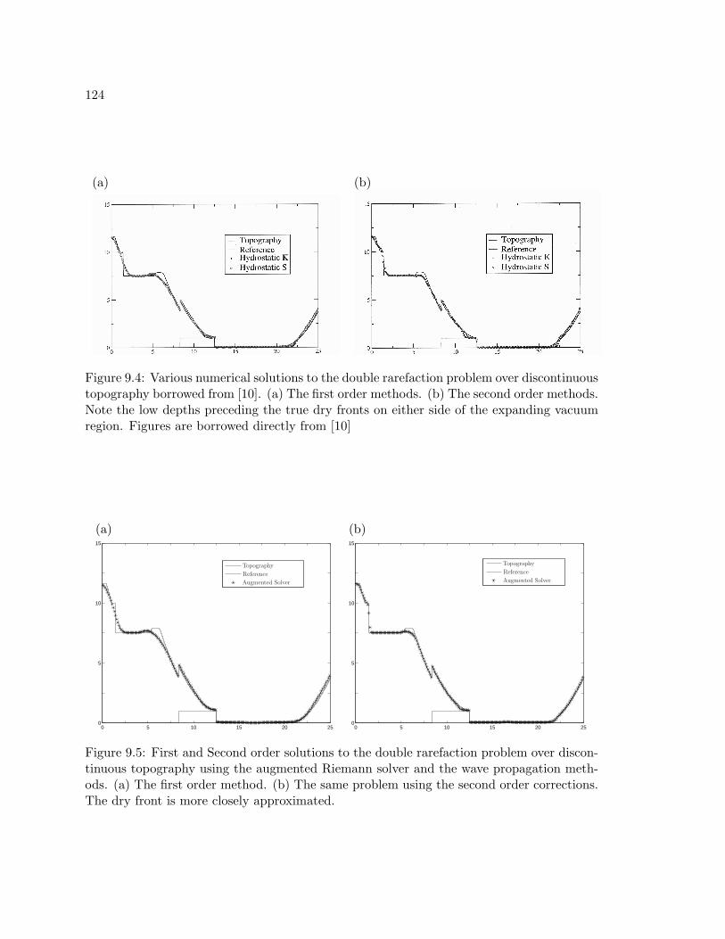
124

(a) (b)

Figure 9.4: Various numerical solutions to the double rarefaction problem over discontinuoustopography borrowed from [10]. (a) The first order methods. (b) The second order methods.Note the low depths preceding the true dry fronts on either side of the expanding vacuumregion. Figures are borrowed directly from [10]

(a) (b)

0 5 10 15 20 250

5

10

15

Topography

Reference

Augmented Solver

0 5 10 15 20 250

5

10

15

Topography

Reference

Augmented Solver

Figure 9.5: First and Second order solutions to the double rarefaction problem over discon-tinuous topography using the augmented Riemann solver and the wave propagation meth-ods. (a) The first order method. (b) The same problem using the second order corrections.The dry front is more closely approximated.

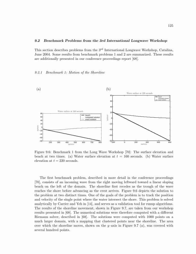
125

9.2 Benchmark Problems from the 3rd International Longwave Workshop

This section describes problems from the 3rd International Longwave Workshop, Catalina,June 2004. Some results from benchmark problems 1 and 2 are summarized. These resultsare additionally presented in our conference proceedings report [68].

9.2.1 Benchmark 1: Motion of the Shoreline

(a) (b)

200 300 400 500 600 700 800−80

−60

−40

−20

0

20

40

60

80beachcomputed solutionexact solution

mete

rs

meters

Water surface at 160 seconds

−200 0 200 400 600 800−80

−60

−40

−20

0

20

40

60

80beachcomputed solutionexact solution

mete

rs

meters

Water surface at 220 seconds

Figure 9.6: Benchmark 1 from the Long Wave Workshop [70]: The surface elevation andbeach at two times. (a) Water surface elevation at t = 160 seconds. (b) Water surfaceelevation at t = 220 seconds.

The first benchmark problem, described in more detail in the conference proceedings[70], consists of an incoming wave from the right moving leftward toward a linear slopingbeach on the left of the domain. The shoreline first recedes as the trough of the wavereaches the shore before advancing as the crest arrives. Figure 9.6 depicts the solution tothe problem at two distinct times. One of the goals of the problem is to track the positionand velocity of the single point where the water intersect the shore. This problem is solvedanalytically by Carrier and Yeh in [14], and serves as a validation tool for runup algorithms.The results of the shoreline movement, shown in Figure 9.7, are taken from our workshopresults presented in [68]. The numerical solutions were therefore computed with a differentRiemann solver, described in [68]. The solutions were computed with 1000 points on amuch larger domain, with a mapping that clustered points near the shoreline. The areaover which the shoreline moves, shown on the y–axis in Figure 9.7 (a), was covered withseveral hundred points.

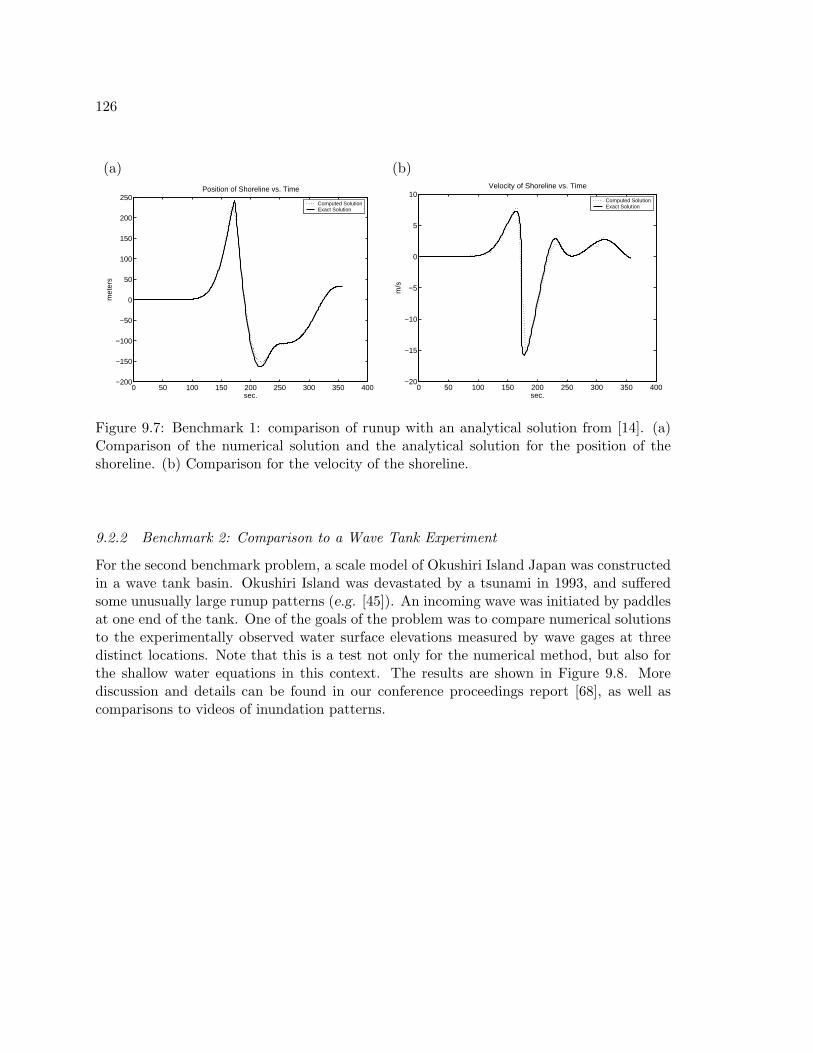
126

(a) (b)

0 50 100 150 200 250 300 350 400−200

−150

−100

−50

0

50

100

150

200

250Position of Shoreline vs. Time

sec.

met

ers

Computed SolutionExact Solution

0 50 100 150 200 250 300 350 400−20

−15

−10

−5

0

5

10Velocity of Shoreline vs. Time

sec.m

/s

Computed SolutionExact Solution

Figure 9.7: Benchmark 1: comparison of runup with an analytical solution from [14]. (a)Comparison of the numerical solution and the analytical solution for the position of theshoreline. (b) Comparison for the velocity of the shoreline.

9.2.2 Benchmark 2: Comparison to a Wave Tank Experiment

For the second benchmark problem, a scale model of Okushiri Island Japan was constructedin a wave tank basin. Okushiri Island was devastated by a tsunami in 1993, and sufferedsome unusually large runup patterns (e.g. [45]). An incoming wave was initiated by paddlesat one end of the tank. One of the goals of the problem was to compare numerical solutionsto the experimentally observed water surface elevations measured by wave gages at threedistinct locations. Note that this is a test not only for the numerical method, but also forthe shallow water equations in this context. The results are shown in Figure 9.8. Morediscussion and details can be found in our conference proceedings report [68], as well ascomparisons to videos of inundation patterns.

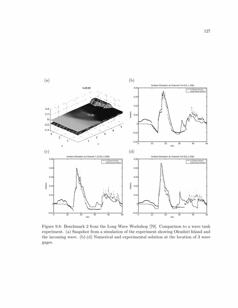
127

(a) (b)

0 10 20 30 40 50−0.02

−0.01

0

0.01

0.02

0.03

0.04Surface Elevation at Channel 5 (4.521,1.196)

sec.

met

ers

Computed SolutionExperimental Solution

(c) (d)

0 10 20 30 40 50−0.01

0

0.01

0.02

0.03

0.04

0.05Surface Elevation at Channel 7 (4.521,1.696)

sec.

met

ers

Computed SolutionExperimental Solution

0 10 20 30 40 50−0.01

0

0.01

0.02

0.03

0.04

0.05Surface Elevation at Channel 9 (4.521,2.196)

sec.

met

ers

Computed SolutionExperimental Solution

Figure 9.8: Benchmark 2 from the Long Wave Workshop [70]. Comparison to a wave tankexperiment. (a) Snapshot from a simulation of the experiment showing Okushiri Island andthe incoming wave. (b)-(d) Numerical and experimental solution at the location of 3 wavegages.

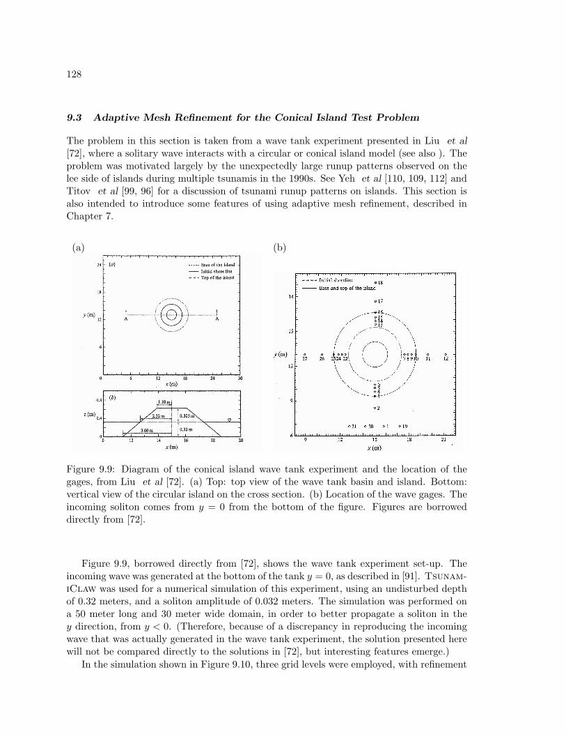
128

9.3 Adaptive Mesh Refinement for the Conical Island Test Problem

The problem in this section is taken from a wave tank experiment presented in Liu et al[72], where a solitary wave interacts with a circular or conical island model (see also ). Theproblem was motivated largely by the unexpectedly large runup patterns observed on thelee side of islands during multiple tsunamis in the 1990s. See Yeh et al [110, 109, 112] andTitov et al [99, 96] for a discussion of tsunami runup patterns on islands. This section isalso intended to introduce some features of using adaptive mesh refinement, described inChapter 7.

(a) (b)

Figure 9.9: Diagram of the conical island wave tank experiment and the location of thegages, from Liu et al [72]. (a) Top: top view of the wave tank basin and island. Bottom:vertical view of the circular island on the cross section. (b) Location of the wave gages. Theincoming soliton comes from y = 0 from the bottom of the figure. Figures are borroweddirectly from [72].

Figure 9.9, borrowed directly from [72], shows the wave tank experiment set-up. Theincoming wave was generated at the bottom of the tank y = 0, as described in [91]. Tsunam-iClaw was used for a numerical simulation of this experiment, using an undisturbed depthof 0.32 meters, and a soliton amplitude of 0.032 meters. The simulation was performed ona 50 meter long and 30 meter wide domain, in order to better propagate a soliton in they direction, from y < 0. (Therefore, because of a discrepancy in reproducing the incomingwave that was actually generated in the wave tank experiment, the solution presented herewill not be compared directly to the solutions in [72], but interesting features emerge.)

In the simulation shown in Figure 9.10, three grid levels were employed, with refinement

129

ratios of 8. The coarsest grid had 1 meter grid cells. The second level tracks the incomingsoliton, and third levels are reserved for capturing the runup at the island, as demonstratedin Figure 9.10. As the soliton wave wraps around the island, maximum runups are observedon the lee side of the island. In [72] this was experimentally reported, but the numericalresults failed to reproduce that observed feature. Figure 9.11 shows the experimentallyrecorded water surface elevation at several gages in the experiment. The locations of thegages are shown in Figure 9.9. These figures are shown to demonstrate some general featuresin the recorded solution. They are not directly compared to the computational results ofthe simulation, since the incoming wave did not replicate the experimental wave exactly.Figure 9.12 shows the numerical solution of TsunamiClaw at locations corresponding togages adjacent to the four sides of the island. Note that the solution at gage 13, locatedon the lee side of the island has the maximum runup. For the location of the gages, seeFigure 9.9.

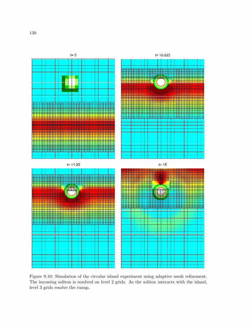
130

Figure 9.10: Simulation of the circular island experiment using adaptive mesh refinement.The incoming soliton is resolved on level 2 grids. As the soliton interacts with the island,level 3 grids resolve the runup.

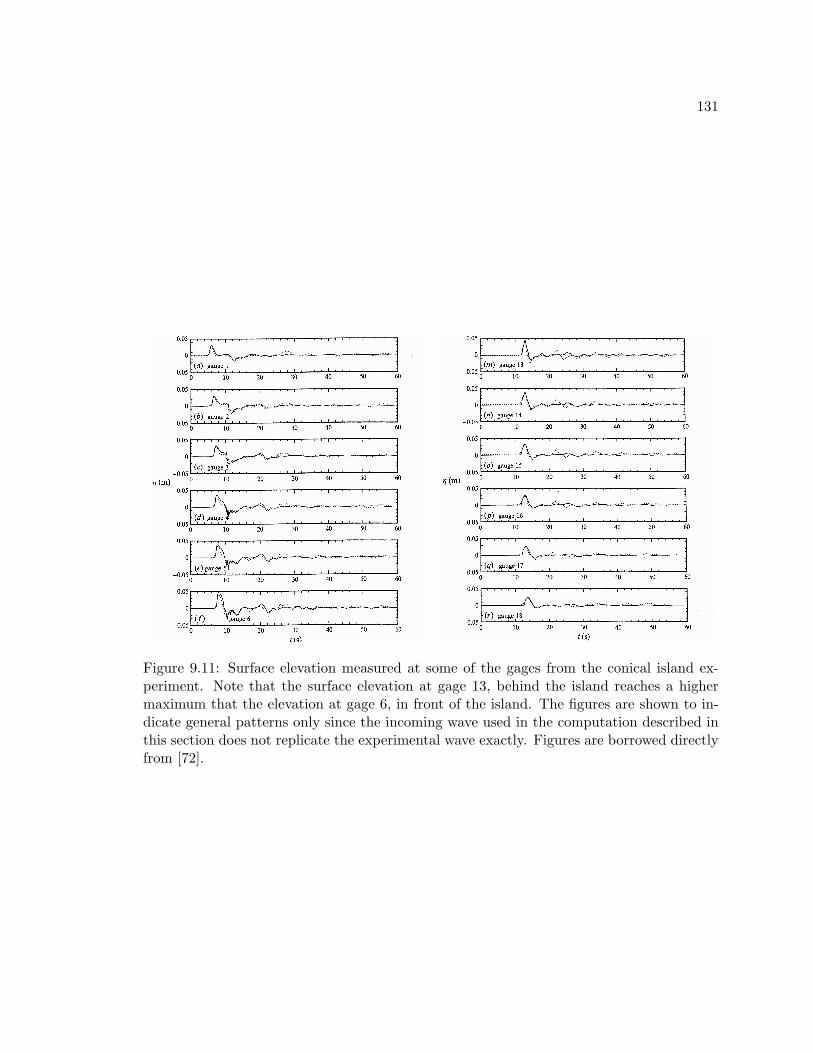
131

Figure 9.11: Surface elevation measured at some of the gages from the conical island ex-periment. Note that the surface elevation at gage 13, behind the island reaches a highermaximum that the elevation at gage 6, in front of the island. The figures are shown to in-dicate general patterns only since the incoming wave used in the computation described inthis section does not replicate the experimental wave exactly. Figures are borrowed directlyfrom [72].

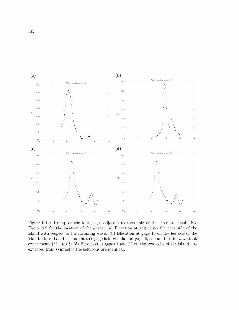
132

(a) (b)

0 5 10 15 20 25−0.01

0

0.01

0.02

0.03

0.04

0.05

0.06Water elevation at gage 6

t

η(t)

0 5 10 15 20 250

0.01

0.02

0.03

0.04

0.05

0.06Water elevation at gage 13

η(t)

(c) (d)

0 5 10 15 20 25−0.01

0

0.01

0.02

0.03

0.04

0.05Water elevation at gage 7

t

η(t)

0 5 10 15 20 25−0.01

0

0.01

0.02

0.03

0.04

0.05Water elevation at gage 22

t

η(t)

Figure 9.12: Runup at the four gages adjacent to each side of the circular island. SeeFigure 9.9 for the location of the gages. (a) Elevation at gage 6 on the near side of theisland with respect to the incoming wave. (b) Elevation at gage 13 on the lee side of theisland. Note that the runup at this gage is larger than at gage 6, as found in the wave tankexperiments [72]. (c) & (d) Elevation at gages 7 and 22 on the two sides of the island. Asexpected from symmetry the solutions are identical.

133

Chapter 10

SIMULATIONS OF THE 2004 INDIAN OCEAN TSUNAMI

In this chapter several TsunamiClaw simulations of the 2004 Indian Ocean Tsunamiwill be shown. The goal of the chapter is to demonstrate the properties and features ofadaptive mesh refinement in the context of a global scale transoceanic tsunami. In all ofthe simulations, dynamic motion of the seafloor bottom was used to generate the tsunami,as described in Section 10.1. The bathymetry in all of the simulations is from the GEBCOdata set, a global one minute gridded data set. For higher grid refinements nautical chartinterpolation was performed where possible. All of the simulations shown were computed ona latitude-longitude spherical grid as described in Chapter 8. Figure 10.1 shows a snapshotfrom a simulation on the Indian Ocean as the tsunami approaches Africa. The figure showsthree levels of grid resolutions, with grid lines omitted from the finest level for clarity. Thecode for all of the simulations shown in this chapter is available at [28].

10.1 The 2004 Sumatra-Andaman Earthquake and Generation of the Tsunami

The 2004 Sumatra-Andaman Earthquake, one of the largest earthquakes in recorded history,initiated the Indian Ocean Tsunami—eventually killing hundreds of thousands of peoplethroughout the Bay of Bengal and Indian Ocean region. The tsunami was the largest inmodern history, and waves spanning the globe and were recorded on every continent (e.g.[95]). The fault rupture initiated on December 26th off the coast of Sumatra and proceedednorth-northwest extending nearly 1300 kilometers along the Andaman islands trough at aspeed of about 2.5 kilometers per second according to Ammon et al [3]. The peak verticalfault displacements are estimated to be approximately 15 meters by the same authors in[3]. Although these fault rupture speeds are fast compared to tsunami propagation (whichcan approach 0.2 kilometers per second), the long duration (about 500 seconds [43]) ofthe fault motion might significantly affect the tsunami wave patterns, as the tsunami mightpropagate upwards of 100 kilometers at the source before the rupture ends. This means thatthe inundation in the islands of Indonesia had begun before the generation of the tsunami1300 kilometers to the north had ended.

10.1.1 Generation with a Spatial-Temporal Model of the Fault Motion

For the above reasons, the simulations shown in this chapter were generated using a dynamicfault model of the spatial-temporal movement of the seafloor. The model was provided bythe Caltech Seismolab, and was generated using the spectral element code specfem3D,described in [54, 55]. The specific data used was Chen Ji’s (Model III), described in [3].The model divides the region surrounding the fault into a 15 minute grid cells and providesdisplacement of the seafloor at 0.1 second intervals for 790 seconds. The simulations shown

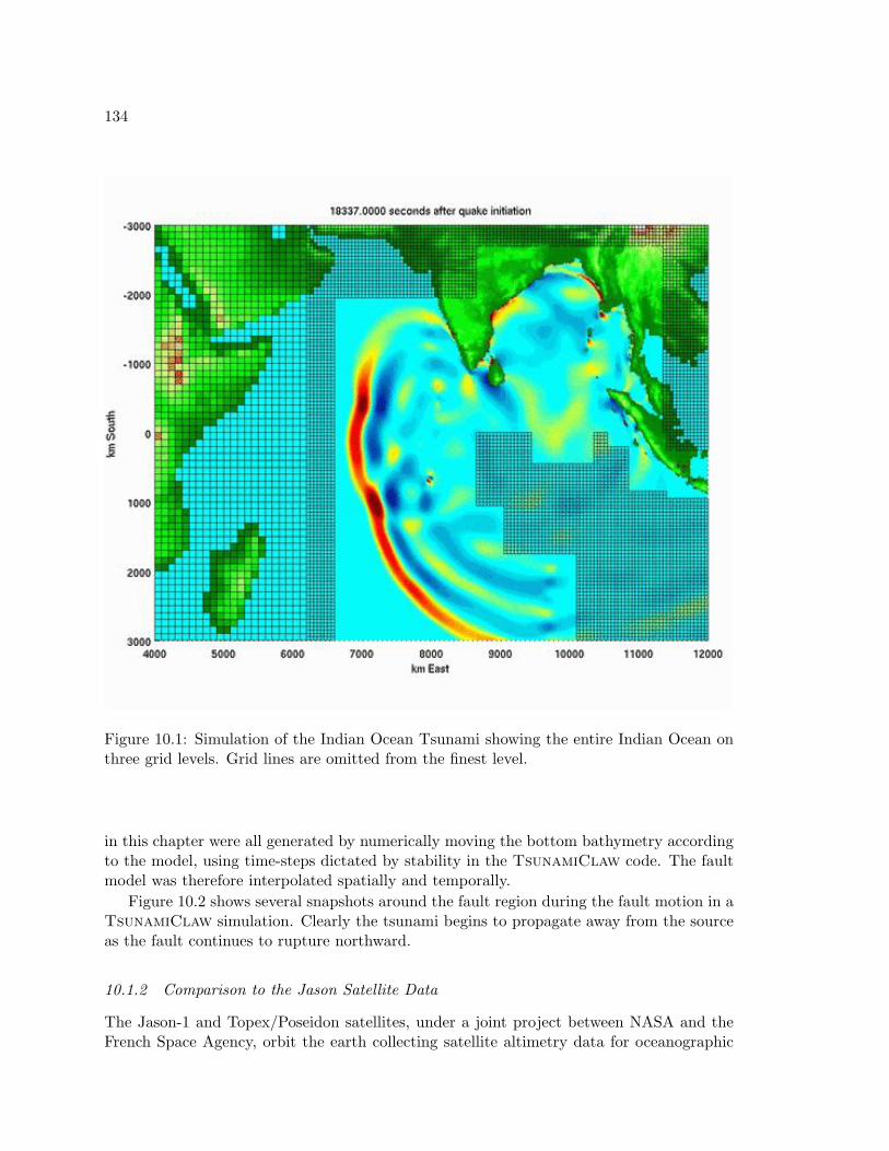
134

Figure 10.1: Simulation of the Indian Ocean Tsunami showing the entire Indian Ocean onthree grid levels. Grid lines are omitted from the finest level.

in this chapter were all generated by numerically moving the bottom bathymetry accordingto the model, using time-steps dictated by stability in the TsunamiClaw code. The faultmodel was therefore interpolated spatially and temporally.

Figure 10.2 shows several snapshots around the fault region during the fault motion in aTsunamiClaw simulation. Clearly the tsunami begins to propagate away from the sourceas the fault continues to rupture northward.

10.1.2 Comparison to the Jason Satellite Data

The Jason-1 and Topex/Poseidon satellites, under a joint project between NASA and theFrench Space Agency, orbit the earth collecting satellite altimetry data for oceanographic

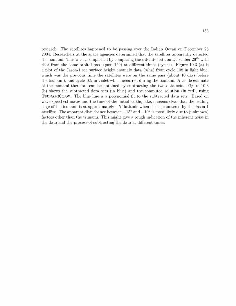
135

research. The satellites happened to be passing over the Indian Ocean on December 262004. Researchers at the space agencies determined that the satellites apparently detectedthe tsunami. This was accomplished by comparing the satellite data on December 26th withthat from the same orbital pass (pass 129) at different times (cycles). Figure 10.3 (a) isa plot of the Jason-1 sea surface height anomaly data (ssha) from cycle 108 in light blue,which was the previous time the satellites were on the same pass (about 10 days beforethe tsunami), and cycle 109 in violet which occurred during the tsunami. A crude estimateof the tsunami therefore can be obtained by subtracting the two data sets. Figure 10.3(b) shows the subtracted data sets (in blue) and the computed solution (in red), usingTsunamiClaw. The blue line is a polynomial fit to the subtracted data sets. Based onwave speed estimates and the time of the initial earthquake, it seems clear that the leadingedge of the tsunami is at approximately −5 latitude when it is encountered by the Jason-1satellite. The apparent disturbance between −15 and −10 is most likely due to (unknown)factors other than the tsunami. This might give a rough indication of the inherent noise inthe data and the process of subtracting the data at different times.

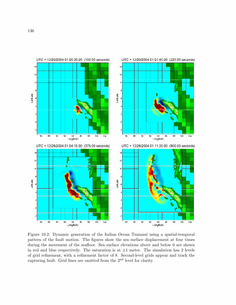
136

Figure 10.2: Dynamic generation of the Indian Ocean Tsunami using a spatial-temporalpattern of the fault motion. The figures show the sea surface displacement at four timesduring the movement of the seafloor. Sea surface elevations above and below 0 are shownin red and blue respectively. The saturation is at ±1 meter. The simulation has 2 levelsof grid refinement, with a refinement factor of 8. Second-level grids appear and track therupturing fault. Grid lines are omitted from the 2nd level for clarity.

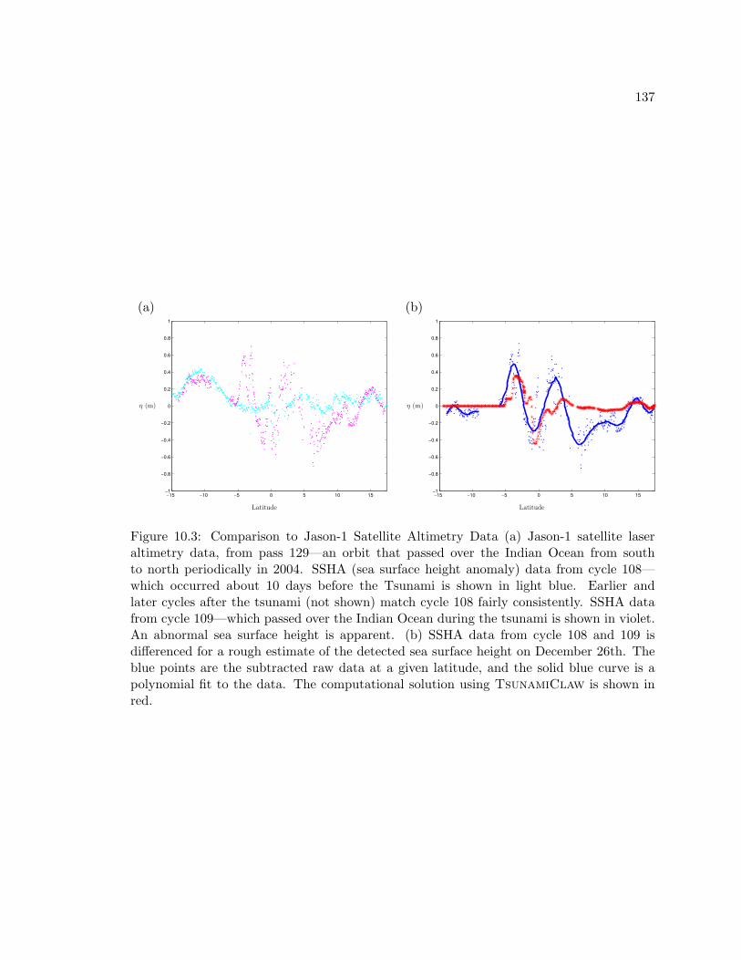
137

(a) (b)

−15 −10 −5 0 5 10 15−1

−0.8

−0.6

−0.4

−0.2

0

0.2

0.4

0.6

0.8

1

PSfrag replacements

Latitude

η (m)

−15 −10 −5 0 5 10 15−1

−0.8

−0.6

−0.4

−0.2

0

0.2

0.4

0.6

0.8

1

PSfrag replacements

Latitude

η (m)

Figure 10.3: Comparison to Jason-1 Satellite Altimetry Data (a) Jason-1 satellite laseraltimetry data, from pass 129—an orbit that passed over the Indian Ocean from southto north periodically in 2004. SSHA (sea surface height anomaly) data from cycle 108—which occurred about 10 days before the Tsunami is shown in light blue. Earlier andlater cycles after the tsunami (not shown) match cycle 108 fairly consistently. SSHA datafrom cycle 109—which passed over the Indian Ocean during the tsunami is shown in violet.An abnormal sea surface height is apparent. (b) SSHA data from cycle 108 and 109 isdifferenced for a rough estimate of the detected sea surface height on December 26th. Theblue points are the subtracted raw data at a given latitude, and the solid blue curve is apolynomial fit to the data. The computational solution using TsunamiClaw is shown inred.

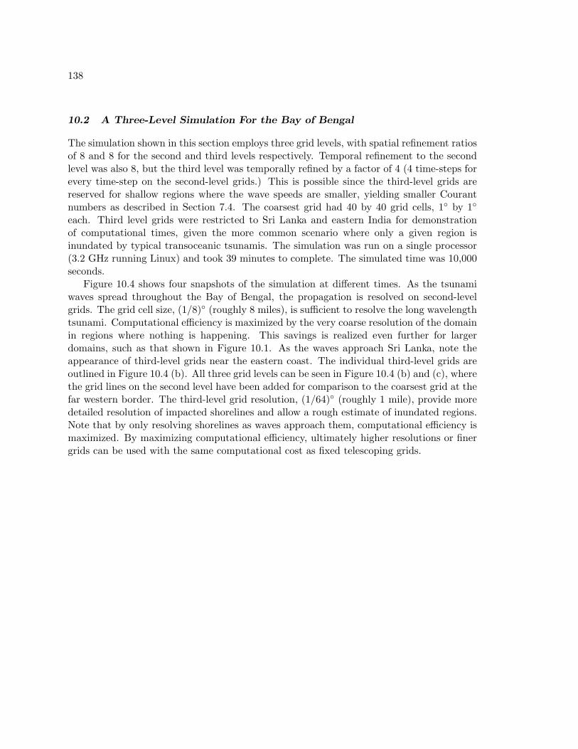
138

10.2 A Three-Level Simulation For the Bay of Bengal

The simulation shown in this section employs three grid levels, with spatial refinement ratiosof 8 and 8 for the second and third levels respectively. Temporal refinement to the secondlevel was also 8, but the third level was temporally refined by a factor of 4 (4 time-steps forevery time-step on the second-level grids.) This is possible since the third-level grids arereserved for shallow regions where the wave speeds are smaller, yielding smaller Courantnumbers as described in Section 7.4. The coarsest grid had 40 by 40 grid cells, 1 by 1

each. Third level grids were restricted to Sri Lanka and eastern India for demonstrationof computational times, given the more common scenario where only a given region isinundated by typical transoceanic tsunamis. The simulation was run on a single processor(3.2 GHz running Linux) and took 39 minutes to complete. The simulated time was 10,000seconds.

Figure 10.4 shows four snapshots of the simulation at different times. As the tsunamiwaves spread throughout the Bay of Bengal, the propagation is resolved on second-levelgrids. The grid cell size, (1/8) (roughly 8 miles), is sufficient to resolve the long wavelengthtsunami. Computational efficiency is maximized by the very coarse resolution of the domainin regions where nothing is happening. This savings is realized even further for largerdomains, such as that shown in Figure 10.1. As the waves approach Sri Lanka, note theappearance of third-level grids near the eastern coast. The individual third-level grids areoutlined in Figure 10.4 (b). All three grid levels can be seen in Figure 10.4 (b) and (c), wherethe grid lines on the second level have been added for comparison to the coarsest grid at thefar western border. The third-level grid resolution, (1/64) (roughly 1 mile), provide moredetailed resolution of impacted shorelines and allow a rough estimate of inundated regions.Note that by only resolving shorelines as waves approach them, computational efficiency ismaximized. By maximizing computational efficiency, ultimately higher resolutions or finergrids can be used with the same computational cost as fixed telescoping grids.

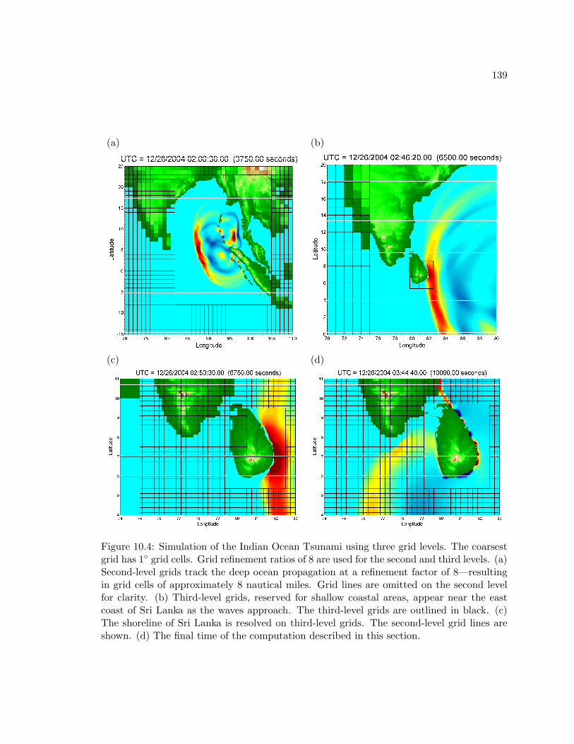
139

(a) (b)

(c) (d)

Figure 10.4: Simulation of the Indian Ocean Tsunami using three grid levels. The coarsestgrid has 1 grid cells. Grid refinement ratios of 8 are used for the second and third levels. (a)Second-level grids track the deep ocean propagation at a refinement factor of 8—resultingin grid cells of approximately 8 nautical miles. Grid lines are omitted on the second levelfor clarity. (b) Third-level grids, reserved for shallow coastal areas, appear near the eastcoast of Sri Lanka as the waves approach. The third-level grids are outlined in black. (c)The shoreline of Sri Lanka is resolved on third-level grids. The second-level grid lines areshown. (d) The final time of the computation described in this section.

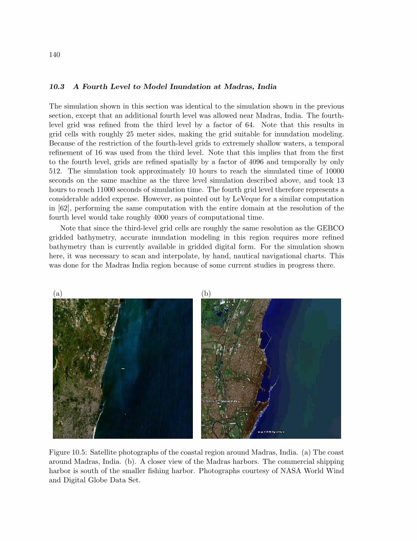
140

10.3 A Fourth Level to Model Inundation at Madras, India

The simulation shown in this section was identical to the simulation shown in the previoussection, except that an additional fourth level was allowed near Madras, India. The fourth-level grid was refined from the third level by a factor of 64. Note that this results ingrid cells with roughly 25 meter sides, making the grid suitable for inundation modeling.Because of the restriction of the fourth-level grids to extremely shallow waters, a temporalrefinement of 16 was used from the third level. Note that this implies that from the firstto the fourth level, grids are refined spatially by a factor of 4096 and temporally by only512. The simulation took approximately 10 hours to reach the simulated time of 10000seconds on the same machine as the three level simulation described above, and took 13hours to reach 11000 seconds of simulation time. The fourth grid level therefore represents aconsiderable added expense. However, as pointed out by LeVeque for a similar computationin [62], performing the same computation with the entire domain at the resolution of thefourth level would take roughly 4000 years of computational time.

Note that since the third-level grid cells are roughly the same resolution as the GEBCOgridded bathymetry, accurate inundation modeling in this region requires more refinedbathymetry than is currently available in gridded digital form. For the simulation shownhere, it was necessary to scan and interpolate, by hand, nautical navigational charts. Thiswas done for the Madras India region because of some current studies in progress there.

(a) (b)

Figure 10.5: Satellite photographs of the coastal region around Madras, India. (a) The coastaround Madras, India. (b). A closer view of the Madras harbors. The commercial shippingharbor is south of the smaller fishing harbor. Photographs courtesy of NASA World Windand Digital Globe Data Set.

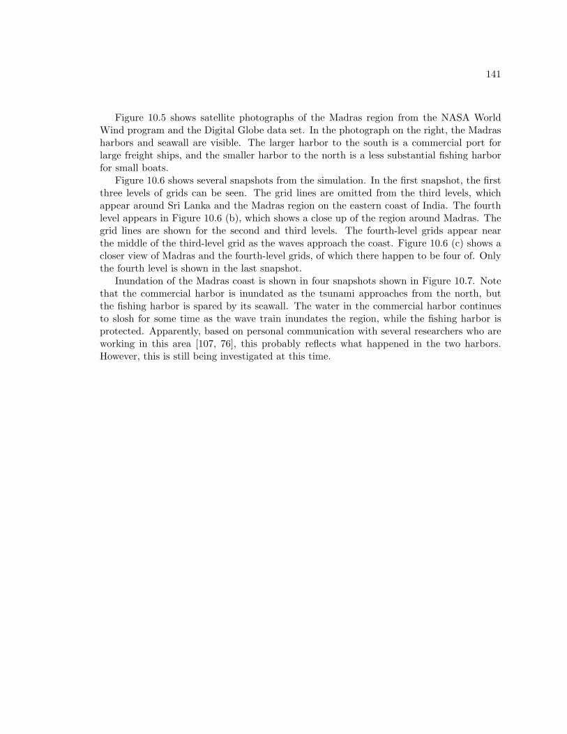
141

Figure 10.5 shows satellite photographs of the Madras region from the NASA WorldWind program and the Digital Globe data set. In the photograph on the right, the Madrasharbors and seawall are visible. The larger harbor to the south is a commercial port forlarge freight ships, and the smaller harbor to the north is a less substantial fishing harborfor small boats.

Figure 10.6 shows several snapshots from the simulation. In the first snapshot, the firstthree levels of grids can be seen. The grid lines are omitted from the third levels, whichappear around Sri Lanka and the Madras region on the eastern coast of India. The fourthlevel appears in Figure 10.6 (b), which shows a close up of the region around Madras. Thegrid lines are shown for the second and third levels. The fourth-level grids appear nearthe middle of the third-level grid as the waves approach the coast. Figure 10.6 (c) shows acloser view of Madras and the fourth-level grids, of which there happen to be four of. Onlythe fourth level is shown in the last snapshot.

Inundation of the Madras coast is shown in four snapshots shown in Figure 10.7. Notethat the commercial harbor is inundated as the tsunami approaches from the north, butthe fishing harbor is spared by its seawall. The water in the commercial harbor continuesto slosh for some time as the wave train inundates the region, while the fishing harbor isprotected. Apparently, based on personal communication with several researchers who areworking in this area [107, 76], this probably reflects what happened in the two harbors.However, this is still being investigated at this time.

142

(a) (b)

(c) (d)

Figure 10.6: Simulation using a fourth-level grid for inundation modeling of the MadrasHarbor. The coarsest grid, seen only on the far left of the top left figure, has 1 grid cells.The second and third grid levels are refined by a factor of 8, and the fourth level is refinedby a factor of 64. (a) Third level grids around Sri Lanka, and Madras, India, are shownwithout grid lines. (b) A closer view of the Madras area. Grid lines are shown on thethird-level grid, and fourth-level grids appear around the Madras area. (c) A closer viewof the fourth-level grids around the Madras harbors as the tsunami approaches. (d) Thefourth-level grids around Madras. The grid resolution is 1/4096 of 1, or approximately 25meters per grid cell.

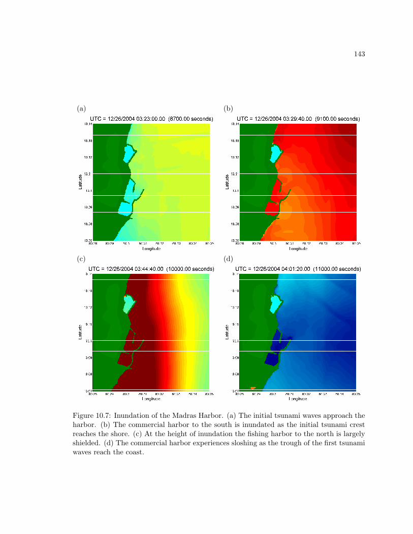
143

(a) (b)

(c) (d)

Figure 10.7: Inundation of the Madras Harbor. (a) The initial tsunami waves approach theharbor. (b) The commercial harbor to the south is inundated as the initial tsunami crestreaches the shore. (c) At the height of inundation the fishing harbor to the north is largelyshielded. (d) The commercial harbor experiences sloshing as the trough of the first tsunamiwaves reach the coast.

144

Chapter 11

CONCLUSIONS AND FUTURE DIRECTIONS

In this chapter a brief summary will be given of the results of this work, and possiblefuture directions will be mentioned.

11.1 Conclusions

In this thesis, various modern Godunov-type numerical methods for hyperbolic PDEs weredeveloped and extended to the application of tsunami modeling. A novel approximateRiemann solver, described in Chapter 6, was developed in order to deal with the diverseflow regimes exhibited by tsunamis. The Riemann solver is based on an overdeterminedor augmented homogeneous system equivalent to the shallow water equations for smoothsolutions. Moreover, the Riemann solver maintained properties of methods that convergeto discontinuous solutions of the shallow water equations for which the overdeterminedhomogeneous system fails to be valid. For instance, the solver was shown to be equivalentto the Roe solver in the event of a single shock-wave solution to a Riemann problem.The solver is well-balanced in terms of integrating the source term, and is particularlyadept at preserving non-stationary steady states, which was shown to be a necessity formodeling transoceanic tsunamis when using Godunov methods for the conservative form ofthe shallow water equations. The solver is depth-positive-definite in the sense of maintainingpositivity of the solution to Riemann problems and is robust and accurate in the presence ofmoving shorelines and evolving dry regions. Although this solver is novel, the goals soughtvery much parallel other recent developments for hyperbolic systems and the shallow waterequations from the hyperbolic numerical community, such as well-balanced solvers thatpreserve positivity.

The wave propagation methods of LeVeque [65, 64], applicable to hyperbolic conserva-tion laws and related nonconservative hyperbolic systems, has been used to implement themethods described in this thesis. The wave propagation methods are particularly suitablefor use with the approximate Riemann solver developed, since the solver is related to anonconservative system. These methods are second-order accurate for smooth solutionsto hyperbolic systems, and maintain the properties necessary to converge to discontinuousweak solutions.

Adaptive refinement algorithms, developed by Berger, Collela, Oliger and LeVeque [7, 9,8] for general hyperbolic systems, were extended and modified to the application of tsunamimodeling with the shallow water equations. This development is believed to be unique in thefield of tsunami modeling, and is thought to be particularly useful due to the diverse scalesof tsunamis. It is believed that adaptive refinement will be an integral piece of tsunamimodeling in the future, particularly if real time tsunami forecasting becomes a tool of thehazard mitigation communities.

145

The goal of this thesis was to lay the groundwork for applying modern Godunov-typefinite volume methods and adaptive refinement to tsunami modeling in a unified and practi-cally useful manner. By dealing with realistic data and scales of tsunamis, many unforseencomplications have been overcome.

11.2 Future Work

11.2.1 Progress in Riemann Solvers for Godunov Methods

Recently there has been rapid progress in the field of Riemann solvers for the shallow waterequations. It is believed that the Riemann solver presented here provides a new simplifiedframework for well-balanced approximate solvers that preserve positivity. It is hoped thatthe resonant problem, where transonic Riemann data occurs in conjunction with variablebathymetry, may be dealt with in a more simplified and coherent manner in the future.It may also be that some of the Riemann solver ideas presented in this thesis may beextendable to other applications, such as gas dynamics, particularly for problems with nearvacuum states.

11.2.2 Adaptive Refinement

Because of the unusual relationship between wave speeds and flow regimes for tsunamis(largest wave speeds occur in the deep ocean near a steady state), the standard time-stepping guidelines for hyperbolic equations, built in to adaptive routines, may be less thanideal for tsunami modeling. It would be useful to have a completely decoupled method,where time-stepping on every grid is determined entirely by stability on that grid, given aproper buffer zone for that grid.

11.2.3 Parallelization

Ideally, the algorithms presented here could be implemented on parallel platforms, allowingmore rapid calculations. For instance, in Section 10.3, it was observed how a fourth-levelgrid slows the computation considerably. Given numerous Cartesian grids with the adaptiverefinement algorithms presented, parallel processing, where different grids are allocated todifferent processors, would be ideal.

11.2.4 Scientific Modeling and Hazard Mitigation

In this thesis, emphasis was placed on the theoretical development of algorithms that arerobust and accurate for solving the shallow water equations when those solutions exhibitdiverse flow features indicative of tsunamis. It has been stated that this thesis is not ascientific investigation of tsunamis. However, the end goal of developing algorithms fortsunami modeling is not to use those algorithms for scientific studies. It is hoped that thealgorithms presented here may form the basis of robust, accurate and user-friendly codesused by tsunami researchers in different arenas.

146

BIBLIOGRAPHY

[1] Y. Agnon, P. Madsen, and H. Schaffer. A new approach to high order Boussinesqmodels. Journal of Fluid Mechanics, 399:319–333, 1999.

[2] I. Aida. Numerical experiments for inundation of tsunamis, Susaki and Usa, in theKochi Prefecture. Bull. Earthq. Res. Inst., 52:441–460, 1977.

[3] C. J. Ammon et al. Rupture process of the 2004 Sumatra-Andaman earthquake.Science, 308:1133–1139, 2005.

[4] M. Arora and P. L. Roe. Postshock oscillations due to shock capturing schemes inunsteady flows. J. Comput. Phys., 130:25–40, 1996.

[5] E. Audeusse, F. Bouchut, M. O. Bristeau, R. Klein, and B. Perthame. A fast andstable well-balanced scheme with hydrostatic reconstruction for shallow water flows.SIAM J. Sci. Comp., 25(6):2050–2065, 2004.

[6] D. Bale, R. J. LeVeque, S. Mitran, and J. A. Rossmanith. A wave-propagation methodfor conservation laws and balance laws with spatially varying flux functions. SIAM J.Sci. Comput., 24:955–978, 2002.

[7] M. J. Berger and P. Colella. Local adaptive mesh refinement for shock hydrodynamics.J. Comput. Phys., 82:64–84, 1989.

[8] M. J. Berger and R. J. LeVeque. Adaptive mesh refinement using wave-propagationalgorithms for hyperbolic systems. SIAM J. Numer. Anal., 35:2298–2316, 1998.

[9] M. J. Berger and J. Oliger. Adaptive mesh refinement for hyperbolic partial differentialequations. J. Comput. Phys., 53:484–512, 1984.

[10] F. Bouchut. Nonlinear Stability of Finite Volume Methods for Hyperbolic ConservationLaws and Well-Balanced Schemes for Sources. Birkhauser Verlag, 2004.

[11] M. Briggs, C. Synolakis, and G. Harkins. Tsunami runup on a conical island. Proc.of Waves—Physical and Numerical Modeling, 1994.

[12] T. Buffard, T. Gallouet, and J. M. Herard. A naive Godunov scheme to solve theshallow water equations. CR Acad. Sci. Paris., 1(326):885–890, 1998.

147

[13] G. Carrier and H. Greenspan. Water waves of finite amplitude on a sloping beach.Journal of Fluid Mech., 62:97–109, 1957.

[14] G. Carrier, T. Wu, and H. Yeh. Tsunami run-up and draw-down on a plane beach.Journal of Fluid Mech., 475:79–99, 2003.

[15] A. Chinnayya and A. Y. LeRoux. A new general Riemann solver for the shallow waterequations with friction and topography. preprint, 2003.

[16] A. Chinnayya, A. Y. LeRoux, and N. Seguin. A well-balanced numerical schemefor the aproximation of the shallow water equations with topgraphy: the resonancephenomenon. to appear in Int. J. Finite Volume, 2004.

[17] V. T. Chow. Open Channel Hydraulics. McGraw-Hill, 1959.

[18] J. F. Colombeau. Multiplication of Distributions: A tool in mathematics, numericalengineering and theoretical physics. Springer Verlag, Berlin, 1992.

[19] G. Dubois and G. Mehlman. A non-parameterized entropy correction for Roe’s ap-proximate riemann solver. Numer. Math., 73:169–208, 1996.

[20] B. Einfeldt. On Godunov-type methods for gas dynamics. SIAM J. Numer. Anal.,25:294–318, 1988.

[21] B. Einfeldt, C. D. Munz, P. L. Roe, and B. Sjogreen. On Godunov-type methods fornear low densities. J. Comput. Phys., 92:273–295, 1991.

[22] J. F. Friedlander and M. Joshi. Introduction to the theory of distributions. CambridgeUniversity Press, 1998.

[23] K. Fujima, M. J. Briggs, and D. Yuliadi. Runup of tsunamis with transient waveprofiles incident on a conical island. Coastal Engineering Journal, 42(2):175–195,2000.

[24] K. Fujima, R. Dozono, and T. Shigemura. Generation and propagation of tsunamiaccompanying edge waves on a uniform sloping shelf. Coastal Engineering Journal,42(2):211–236, 2000.

[25] K. Fujima, K. Masamura, and C. Goto. Generation and propagation of tsunamiaccompanying edge waves on a uniform sloping shelf. Coastal Engineering Journal,44(4):373–397, 2002.

[26] T. Gallouet, J. M. Herard, and N. Seguin. Some approximate Godunov schemes tocompute shallow water equations with topography. Computers and Fluids, 32:479–513, 2003.

148

[27] P. Garcıa-Navarro and M. E. Vazques-Cendon. On numerical treatment of the sourceterms in the shallow water equations. Comput. Fluids, 29:17–45, 2000.

[28] D. L. George. Website url. http://www.amath.washington.edu/~dgeorge.

[29] D. L. George. Numerical approximation of the nonlinear shallow water equations: aGodunov-type scheme. Master’s thesis, University of Washington, 2004.

[30] G. Gisler, R. Weaver, C. Mader, and M. Gittings. Two- and three-dimensional simu-lations of asteroid ocean impacts. Science of Tsunami Hazards, 21:119.

[31] M. Gobbi, J. Kirby, and G. Wei. A fully nonlinear Boussinesq model for surface waves.part ii. extension to o(kh)4. Journal of Fluid Mechanics, 405:182–210, 2000.

[32] E. Godlewski and P. Raviart. Numerical Approximation of Hyperbolic Systems ofConservation Laws. Springer, New York, 1996.

[33] S. K. Godunov. A difference method for numerical calculation of discontinuous solu-tions of the equations of hydrodynamics. Mat. Sb., 47:271–306, 1959.

[34] F. Gonzalez and Y. Kulikov. Tsunami dispersion observed in the deep ocean.Tsunamis in the World, pages 7–16, 1993.

[35] L. Gosse. Localization effects and measure source terms in numerical schemes forbalance laws. Math. Comp., 71:553–582, 2002.

[36] C. Goto and K. Sato. Development of tsunami numerical simulation system for Sanrikucoast in Japan. Rep. Port Harbor Res. Inst., 32(2):3–44, 1993. In Japanese.

[37] N. Goutal and F. Maurel. Proceedings of the second workshop on dam-break wavesimulation. Technical report, Chatou, France, 1997. EDF/DER HE-43/97/016/B.

[38] J. M. Greenberg and A. Y. LeRoux. A well-balanced scheme for numerical processingof source terms in hyperbolic equations. SIAM Journal of Numerical Analysis, 33:1–16, 1996.

[39] J. M. Greenberg, A. Y. LeRoux, R. Barraille, and A. Noussair. Analysis and ap-proximantion of conservation laws with source terms. SIAM Journal of NumericalAnalysis, 34:1980–2007, 1997.

[40] A. Harten. High resolution shcemes for hyperblic conservation laws. J. Comput. Phys.,49:357–393, 1983.

149

[41] A. Harten and J. M. Hyman. Self-adjusting grid methods for one-dimensional hyper-bolic conservation laws. J. Comput. Phys., 50:235–269, 1983.

[42] A. Harten, P. D. Lax, and B. van Leer. On upstream differencing and Godunov-tpyeschemes for hyperbolic conservation laws. SIAM Review, 25:235–61, 1983.

[43] D. Helmberger, S. Ni, and H. Kanamori. Energy radiation form the Sumatra earth-quake. Nature, 434:582–583, 2005.

[44] S. Hibberd and D. H. Peregrine. Surf and run-up on a beach: a uniform bore. Journalof Fluid Mech., 95:323–345, 1979.

[45] 1993 HOKKAIDO TSUNAMI SURVEY GROUP. Tsunami devastates Japanesecoastal region. EOS Trans. AGU, 74(37), 1993.

[46] J. Horillo, Z. Kowalik, and S. Yoshinori. Wave dispersion study in the Indian OceanTsunami of december 26, 2004. Science of Tsunami Hazards, 25(1):42–63, 2006.

[47] T. Hou and P. LeFloch. Why non-conservative schemes converge to the wrong solu-tions: Error analysis. Math. of Comput., 62:497–530, 1994.

[48] F. Imamura. Review of tsunami simulation with a finite difference method. Long-WaveRunup Models, pages 25–42, 1996.

[49] S. Jin and X. P. Xin. The relaxation schemes for systems of conservation laws inarbitrary space dimensions. Comm. Pure Appl. Math., 48(235), 1995.

[50] R. Johnson. A Modern Introduction to the Mathematical Theory of Water Waves.Cambridge University Press, 1997.

[51] S. Karni and S. Canic. Computations of slowly moving shocks. J. Comput. Phys.,136:132–139, 1997.

[52] T. Katsaounis, B. Perthame, and C. Simeoni. Upwinding sources at interfaces inconservation laws. to appear in Appl. Math. Lett.

[53] A. Kennedy, J. Kirby, Q. Chen, and R. Dalrymple. Boussinesq type equations withimproved nonlinear behavior. Wave Motion, 33:225–243, 2001.

[54] D. Komatitsch and J. Tromp. Spectral-element simulations of global seismic wavepropagation I. Geophysical Journal International, 149:390–412, 2002.

[55] D. Komatitsch and J. Tromp. Spectral-element simulations of global seismic wavepropagation II. three-dimensional models, oecans, rotation and self-gravitation. Geo-physical Journal International, 150:303–318, 2002.

150

[56] Z. Kowalik, W. Knight, T. Logan, and P. Whitmore. Modeling of the global tsunami:Indonesian Tsunami of 26 December 2004. Science of Tsunami Hazards, 23(1):40–56,2005.

[57] E. Kulikov, A. B. Rabinovich, R. Thomson, and B. Bornhold. The landslide tsunamiof November 3, 1994, Skagway Harbor, Alaska. Journal of Geophysical Research,101(C3):6609–6616, 1996.

[58] Y. Kulikov. The highly dispersive waves of the Indian Ocean Tsunami. RussianAcademy of Sciences, 2005.

[59] A. Kurganov and D. Levy. Central upwind schemes for the St. Venant system. Math-ematical Modelling and Numerical Analysis, 36:397–425, 2002.

[60] P. D. Lax and B. Wendroff. Systems of conservation laws. Comm. Pure Appl. Math,13:217–237, 1960.

[61] R. J. LeVeque. Clawpack software. http://www.amath.washington.edu/~claw.

[62] R. J. LeVeque. Wave propagation software, computational science, and reproducibleresearch. Proceedings of the International Congress of Mathematicians, page to ap-pear.

[63] R. J. LeVeque. High resolution finite volume methods on arbitrary grids via wavepropagaton. Journal of Computational Physics, 78:36–63, 1988.

[64] R. J. LeVeque. Numerical Methods For Conservation Laws. Birkhauser-Verlag, 1990.

[65] R. J. LeVeque. Wave propagation algorithms for multi-dimensional hyperbolic sys-tems. Journal of Computational Physics, 131:327–335, 1997.

[66] R. J. LeVeque. Balancing source terms and flux gradients in high-resolution Godunovmethods: The quasi-steady wave propagation algorithm. Journal of ComputationalPhysics, 146:346–365, 1998.

[67] R. J. LeVeque. Finite Volume Methods For Hyperbolic Problems. Cambridge Univer-sity Press, 2002.

[68] R. J. LeVeque and D. L. George. High-resolution finite volume methods for the shallowwater equations with bathymetry and dry states. In P. Liu, editor, Proceedings ofLong-Wave Workshop, Catalina, page to appear, 2004.

[69] R. J. LeVeque and M. Pelanti. A class of approximate Riemann solvers and theirrelation to relaxation schemes. Journal of Computational Physics, 172:572–591, 2001.

151

[70] P. Liu, editor. Proceedings of the 3rd International Long-Wave Workshop, Catalina,Catalina Island, California, 2004.

[71] P. L. Liu and Y. S. Cho. An integral equation model for for wave propagation withbottom frictions. J. Waterway, Port, Coastal, Ocean Engng., ASCE, 120:594–608,1994.

[72] P. L. Liu, Y. S. Cho, M. Briggs, U. Kanoglu, and C. Synolakis. Runup of solitarywaves on a circular island. Journal of Fluid Mech., 302:259–285, 1995.

[73] C. L. Mader. Numerical Modeling of Water Waves. CRC Press, 2004.

[74] P. Madsen, H. Bingham, and H. Liu. A new Boussinesq method for fully nonlinearwaves from shallow to deep water. Journal of Fluid Mechanics, 462:1–30, 2002.

[75] P. Madsen and O. Sorensen. A new form of the Boussinesq equations with improvedlinear dispersion. Coastal Engineering, pages 183–204, 1992.

[76] T. S. Murty, 2006. Personal Communication.

[77] S. Noelle, N. Pankratz, G. Puppo, and J. R. Natvig. Well-balanced finite volumeschemes of arbritrary order of accuracy for shallow water flows. J. Comput. Phys.,213:474–499, 2006.

[78] O. Nwogu. Alternative form of the Boussinesq equations for nearshore wave propa-gation. Journal of Waterway, Port, Coastal, and Ocean Engineering, 119(6):618–638,1993.

[79] National Oceanographic and Atmospheric Administration. NOAA Center for TsunamiResearch. http://www.http://nctr.pmel.noaa.gov/.

[80] D. H. Peregrine. Long waves on a beach. Journal of Fluid Mechanics, 27(4):815–827,1967.

[81] P. Rivera. Modeling the Asian tsunami evolution and propagation with a new genera-tion mechanism and a nonlinear dispersive wave model. Science of Tsunami Hazards,25(1):18–33, 2006.

[82] P. L. Roe. Approximate Riemann solvers, parameter vectors, and difference schemes.J. Comput. Phys., 43:357–372, 1981.

[83] P. L. Roe. Upwind differencing schemes for hyperbolic conservation laws with sourceterms., volume 1270 of Lecture Notes in Math, pages 41–51. Springer-Verlag, 1987.

152

[84] J. A. Rossmanith. A Wave Propagation Method with Constrained Transport for idealand shallow water magnetohydrodynamics. PhD thesis, University of Washington,2002.

[85] J. A. Rossmanith, D. S. Bale, and R. J. LeVeque. A wave propagation algorithm forhyperbolic systems on curved manifolds. J. Comput. Phys., 199:631–662, 2004.

[86] K. Sitanggang and P. Lynett. Parallel computation of a highly nonlinear boussinesqequation model through domain decomposition. International Journal for NumericalMethods in Fluids, In Press, 2005.

[87] J. J. Stoker. Water Waves:The Mathematical Theory with Applications. IntersciencePublishers, New York, 1957.

[88] G. Strang. On construction and comparison of difference schemes. SIAM J. Numer.Anal., pages 506–517, 1968.

[89] P. K. Sweby. High resolution schemes using flux limiters for hyperbolic conservationlaws. SIAM Journal of Numerical Analysis, 21:995–1011, 1984.

[90] C. E. Synolakis. The runup of solitary waves. J. Fluid Mech., 185:523–545, 1987.

[91] C. E. Synolakis. Generation of long waves in the laboratory. J. Waterways, Port,Coastal, Ocean Engng. ASCE, 116:252–266, 1990.

[92] C. E. Synolakis, P. Liu, G. Carrier, and H. Yeh. Tsunamigenic sea-floor deformations.Science, 278:598–600, 1997.

[93] V. V. Titov. Numerical Modeling of Long Wave Runup. PhD thesis, University ofSouthern California, 1997.

[94] V. V. Titov and F. I. Gonzalez. Implementation and testing of the method of splittingtsunami (MOST) model. NOAA Technical Memorandum ERL PMEL-112.

[95] V. V. Titov, A. B. Rabinovich, H. O. Mofjeld, R. E. Thomson, and F. I. Gonzalez. Theglobal reach of the 26 December 2004 Sumatra Tsunami. Science, 309(5743):2045–2048.

[96] V. V. Titov and C. E. Synolakis. Extreme inundation flows during the Hokkaido-Nansei-Oki Tsunami. Geophys. Res. Lett., 24(11):1315–1318.

[97] V. V. Titov and C. E. Synolakis. Modeling of breaking and nonbreaking long waveevolution and runup using VTCS-2. Jounal of Waterways, Ports, Coastal and OceanEngineering, 121(6):308–316.

153

[98] V. V. Titov and C. E. Synolakis. Numerical modeling of tidal wave runup. Jounal ofWaterways, Ports, Coastal and Ocean Engineering, 124(4):157–171.

[99] V. V. Titov and C. E. Synolakis. A numerical study of wave runup of the September 2,1992 Nicaraugan tsunami. Tsunami 93 Proc. IUGG/IOC Intl Tsunami Symp., pages627–636, 1993.

[100] E. F. Toro. Riemann Solvers and Numerical Methods for Fluid Dynamics. Springer–Verlag, Berlin, 1997.

[101] E. F. Toro. Shock Capturing Methods for Free Surface Shallow Flows. John Wileyand Sons, Chichester,United Kingdom, 2001.

[102] R. Walters. A semi-implicit finite element model for non-hydrostatic (dispersive)surface waves. International Journal for Numerical Methods in Fluids, 7:721–737,2005.

[103] G. Whitham. Linear and Nonlinear Waves. John Wiley and Sons, New York, 1974.

[104] H. Yeh. Nonlinear progressive edge waves: Their instability and evolution. Journalof Fluid Mechanics, 152:479–499, 1985.

[105] H. Yeh. Experimental study of standing edge waves. Journal of Fluid Mechanics,168:291–304, 1986.

[106] H. Yeh. Free-surface dynamics. In P. L. F. Liu, editor, Advances in Coastal and OceanEngineering, volume 1, pages 1–75, 1994.

[107] H. Yeh, 2006. Personal Communication.

[108] H. Yeh, Ghazali A., and I. Marton. Experimental study of bore runup. Journal ofFluid Mechanics, 206:563–578, 1989.

[109] H. Yeh, F. Imamura, C. E. Synolakis, Y. Tsuji, P. Liu, and S. Shi. The Flores Islandtsunamis. EOS, Trans. AGU, 74(33)(369):371–373, 1993.

[110] H. Yeh, P. Liu, M. Briggs, and C. Synolakis. Propagation and amplification oftsunamis at coastal boundaries. Nature, 372:353–355, 1994.

[111] H. Yeh and K. M. Mok. On turbulence in bores. Physics of Fluids, 2:821–828, 1990.

[112] H. Yeh, V. Titov, V. Gusiakov, E. Pelinovsky, V. Khramushin, and V. Kaistrenko.The Shikotan earthquake tsunamis. Pure. Appl. Geophys., 1995.

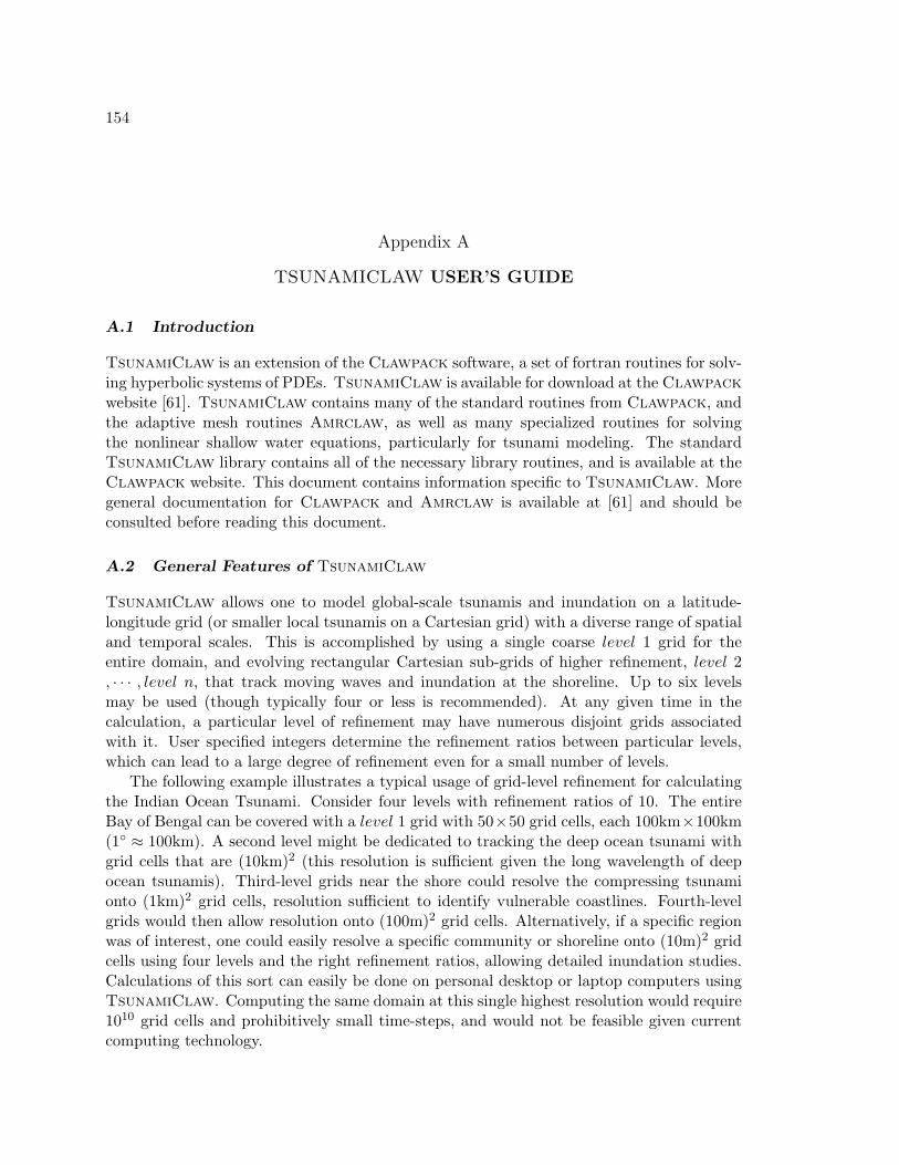
154

Appendix A

TSUNAMICLAW USER’S GUIDE

A.1 Introduction

TsunamiClaw is an extension of the Clawpack software, a set of fortran routines for solv-ing hyperbolic systems of PDEs. TsunamiClaw is available for download at the Clawpackwebsite [61]. TsunamiClaw contains many of the standard routines from Clawpack, andthe adaptive mesh routines Amrclaw, as well as many specialized routines for solvingthe nonlinear shallow water equations, particularly for tsunami modeling. The standardTsunamiClaw library contains all of the necessary library routines, and is available at theClawpack website. This document contains information specific to TsunamiClaw. Moregeneral documentation for Clawpack and Amrclaw is available at [61] and should beconsulted before reading this document.

A.2 General Features of TsunamiClaw

TsunamiClaw allows one to model global-scale tsunamis and inundation on a latitude-longitude grid (or smaller local tsunamis on a Cartesian grid) with a diverse range of spatialand temporal scales. This is accomplished by using a single coarse level 1 grid for theentire domain, and evolving rectangular Cartesian sub-grids of higher refinement, level 2, · · · , level n, that track moving waves and inundation at the shoreline. Up to six levelsmay be used (though typically four or less is recommended). At any given time in thecalculation, a particular level of refinement may have numerous disjoint grids associatedwith it. User specified integers determine the refinement ratios between particular levels,which can lead to a large degree of refinement even for a small number of levels.

The following example illustrates a typical usage of grid-level refinement for calculatingthe Indian Ocean Tsunami. Consider four levels with refinement ratios of 10. The entireBay of Bengal can be covered with a level 1 grid with 50×50 grid cells, each 100km×100km(1 ≈ 100km). A second level might be dedicated to tracking the deep ocean tsunami withgrid cells that are (10km)2 (this resolution is sufficient given the long wavelength of deepocean tsunamis). Third-level grids near the shore could resolve the compressing tsunamionto (1km)2 grid cells, resolution sufficient to identify vulnerable coastlines. Fourth-levelgrids would then allow resolution onto (100m)2 grid cells. Alternatively, if a specific regionwas of interest, one could easily resolve a specific community or shoreline onto (10m)2 gridcells using four levels and the right refinement ratios, allowing detailed inundation studies.Calculations of this sort can easily be done on personal desktop or laptop computers usingTsunamiClaw. Computing the same domain at this single highest resolution would require1010 grid cells and prohibitively small time-steps, and would not be feasible given currentcomputing technology.

155

TsunamiClaw is based on a finite volume numerical method, which means that thesolution is represented as a piecewise constant, with numerical values approximating theaverage solution value in each discrete computational grid cell. There is no specific referenceto the shoreline—grid cells may simply be wet or dry depending on their location, and mayfill-up or drain-out of water as waves inundate or draw-down at the shoreline. This meansthat dry land is part of the computational domain, and a single grid is a simple rectanglethat may overlap the shoreline. TsunamiClaw solves the shallow water equations in theirphysically relevant conservative form, therefore, the solution is represented as water depthand momentum. This is one feature that allows convergence to discontinuous bores. See[67] and [8] for a mathematical descriptions of these methods.

A.3 Running TsunamiClaw

This document assumes a basic working knowledge of Unix or Linux. TsunamiClaw iswritten in fortran 77, and can be run on any system with a proper fortran compiler. However,using the provided Makefiles requires that you are using a Unix or Linux operating system.TsunamiClaw consists of a directory of library routines, as well as an application directorythat will be used to specify problem specific parameters. Routines in the library shouldtypically not require any modification, and should only be modified at your own risk. (Onepossible exception is the call.i file. See the standard Clawpack documentation).

A.4 The TsunamiClaw library

The standard TsunamiClaw library,tsunamiclaw/lib,

is available at the Clawpack website as a tar-zipped directory,tsunamiclaw.tar.gz.

On your system, the unzipped directory should be in a path specified by an environmentvariable that you should name TSUNAMICLAW. The path to the TsunamiClaw library willtherefore be referred to as,

$TSUNAMICLAW/lib.It is recommended to set this environment variable in one of your login scripts (such as.cshrc or .bashrc depending on your shell). Before using TsunamiClaw, the .f fortranfiles in the library must be made into .o object files. This can be done by typing “make”from the library directory

$TSUNAMICLAW/lib.(Note: the variable TSUNAMICLAW must be set before using make.) If the library is modified(not recommended), or moved from one system to another, make should be run again.

The TsunamiClaw library contains a mix of routines, some that are unique and somethat are standard routines of Clawpack and Amrclaw. Routines that are unique to theTsunamiClaw library are named by the convention filename_tc.f. Other versions fromthe standard Clawpack library may or may not be compatible with the filename_tc.froutines. Use caution if updating to newer versions of the Clawpack or Amrclaw libraries.

156

A.5 Application Directory

TsunamiClaw will be run from an application directory that may reside anywhere inyour directory structure. An application directory will contain input data files where pa-rameters will be set for each specific problem. TsunamiClaw uses two input data files,amr2ez.data and setprob.data. Standard Clawpack computational parameters are setin amr2ez.data, such as the physical domain and refinement parameters, and the other file,setprob.data, is used to set computational parameters specific to TsunamiClaw. Theapplication directory will also contain several required fortran routines (.f files), explainedin section section A.8, that can optionally be modified to your needs. However, for standardapplications it should only be necessary to set parameters in the input data file. To makethe executable that runs TsunamiClaw, type “make xtsunami” from the application di-rectory. The executable file xtsunami can then be run from this directory. An exampleapplication directory comes with TsunamiClaw,

$TSUNAMICLAW/tc example,that contains the required fortran routines (.f files) and the input files (.data files), as wellas some matlab plotting scripts (.m files). It is recommended that you copy this directoryto another location outside of $TSUNAMICLAW before making modifications, so that if youupdate TsunamiClaw to newer versions, your personal application directories will not beoverwritten.

A.6 Data Input (setprob.data)

The computational parameters set in setprob.data are described below. Note that integervariables start with the letters m or l, so values specified in setprob.data for these variablesshould not contain any decimal points.

gravity: The gravitational constant should typically be set to 9.8, unless units other thanmeters and seconds are desired. When using the default latitude-longitude units,internal calculations rely on meters as the physical units, so the default value of 9.8should be used.

depthtolerance: Water depths below this value (in meters) will be effectively treatedas zero. This makes the computation more efficient, since it prevents computing thesolution in areas with vanishingly small depths. It is recommended to use a reasonablevalue such as 10−3 (1 millimeter) or larger. Since the shallow water equations haveno viscosity, water velocities can be unrealistically large in regions with very shallowdepths, and this can lead to inefficient time-stepping or even instabilities. (Note thatfriction can help alleviate this problem.) Using a value in the range of 10−3 to 10−2

is recommended.

shallowdepth: This parameter is used for refinement purposes. Typically more refinementis desired, and needed due to decreasing wavelengths, in shallow coastal waters. Thisparameter indicates areas that are considered “shallow” in meters. Larger values will

157

lead to larger areas of refinement, while smaller values will lead to limited refinementareas closer to shore. A typical value might be 100 (meters). See maxdeepoceanlevelbelow.

wavetolerance: This parameter is used for refinement purposes near waves, and controlshow sensitive refinement is to deviations from level sea-surface. Smaller values willtherefore lead to larger areas of refinement and larger values will lead to smaller areasof refinement surrounding only the biggest waves. Since deep ocean tsunamis do notnecessarily have large amplitudes, a value such as 10−1 (10 cm) might be a typicalvalue for a global scale tsunami.

frictioncoeff: This parameter sets the Manning coefficient used for optional bottomfriction. Bottom friction may be important for realistic run-up heights and can speedcalculation times as well. The friction formula is a standard empirically derived for-mula. Higher values of the Manning coefficient correspond to greater friction. Atypical value used in a tsunami calculation might be 0.025. For friction, the source-term splitting option must be set in amr2ez.data. If you do not want to use friction,you can set frictioncoeff to 0.0, or turn-off source term integration in amr2ez.data.

maxdeepoceanlevel: This parameter determines what level of refinement is allowed in thedeep ocean. Typically deep ocean tsunamis have very long wavelengths, and so highlevels of refinement are not needed and would be computationally wasteful in thedeep ocean. A typical computation might only allow the second level of refinementin the deep ocean, reserving higher level grids for shallow regions near the shore. Forclassification of deep and shallow TsunamiClaw uses the shallowdepth parameter.

levelallowdomain: This parameter determines what level of refinement is allowed on theentire domain. For instance, it might be desired to restrict high levels of refinement tocertain regions of the domain. In this case levelallowdomain should be set to somelower value that is allowed on the entire domain. See below for parameters that allowhigher refinement in certain regions.

methodquake: This parameter determines the type of method that is to be used to gener-ate the tsunami. It can have integer values of 0,1, or 2. If methodquake= 2, then adynamic fault model is used, as specified in a user provided data file. If methodquake= 1, then a static initial condition is used, as specified in a user provided data file. Theformats for these files are described in the section “Fault Models”. If methodquake= 0then the user must provide some other means of generating the tsunami, such as spec-ifying an initial condition directly in qinit.f, or perhaps a user specified boundarycondition. To use these latter options, see the standard Clawpack documentation.

158

minfaultrefinelevel: This parameter is used for determining refinement in the regiondescribed by the fault model. It can have any integer value up to the number of refine-ment levels specified in amr2ez.data. Setting mfaultrefinelevel= n will enforcethat level n grids or finer will cover the fault region during the fault motion. If you donot want to enforce a particular level, but wish for TsunamiClaw to treat the faultregion like any other region, refining based on wave heights and water depths, thenset mfaultrefinelevel to a low value such as 0 or 1.

faultfname: On the line following mfaultrefinelevel, you should place the relative orfull path to the file of the fault model in single quotes. If methodquake= 0, then theline should be blank.

mbathfiles: Set mbathfiles to the integer number of bathymetry files that you wouldlike to read in. If you are specifying bathymetry directly by some other means, setmathfiles = 0. See the description of setaux.f.

levelallowbathfile(mbathfiles): This line should contain a list of mbathfiles integers,specifying the level of refinement allowed over each bathymetry file to be used. Thisvariable is useful if you would like to use a certain level of refinement over most ofthe domain, yet reserve high levels of refinement for regions where you have moredetailed bathymetry. For more about how bathymetry files can be used, see thesection Bathymetry.

bathfname(mbathfiles): The next mbathfiles lines should contain the paths to thebathymetry files in single quotes. There should be at least one, unless mbathfiles= 0, in which case the line should be empty. The order that they are listed in shouldcorrespond to values specified in the list of integers.

mregions: For additional control and restriction of refinement to particular regions, setmregions to an integer number of regions that you would like to specify.

levelallowregion(mregions): This line should contain a list of mregions integers, spec-ifying the level of refinement allowed over each region to be specified. This option isuseful if you would like use high levels of refinement for regions of interest, even ifthese regions do not correspond specifically to bathymetry files.

regioncoords(4,mregions): The next mregions lines should each contain a list of fourcoordinates specifying the particular region: xlower xupper ylower yupper.

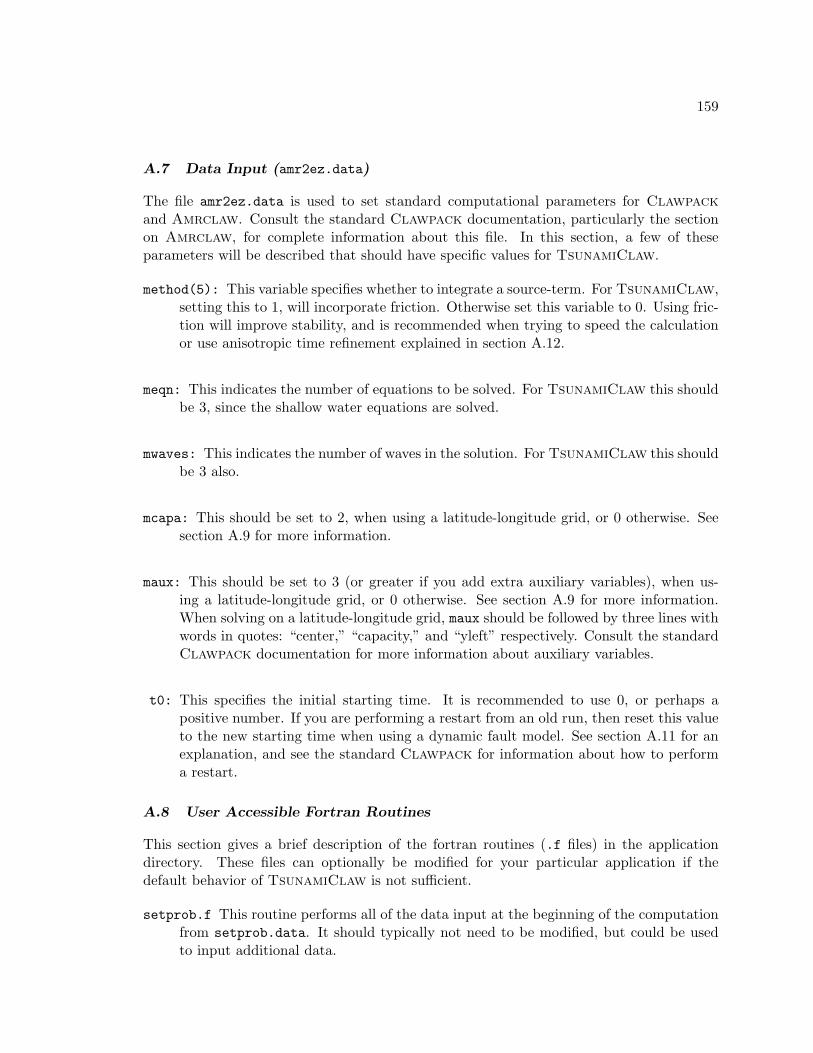
159

A.7 Data Input (amr2ez.data)

The file amr2ez.data is used to set standard computational parameters for Clawpackand Amrclaw. Consult the standard Clawpack documentation, particularly the sectionon Amrclaw, for complete information about this file. In this section, a few of theseparameters will be described that should have specific values for TsunamiClaw.

method(5): This variable specifies whether to integrate a source-term. For TsunamiClaw,setting this to 1, will incorporate friction. Otherwise set this variable to 0. Using fric-tion will improve stability, and is recommended when trying to speed the calculationor use anisotropic time refinement explained in section A.12.

meqn: This indicates the number of equations to be solved. For TsunamiClaw this shouldbe 3, since the shallow water equations are solved.

mwaves: This indicates the number of waves in the solution. For TsunamiClaw this shouldbe 3 also.

mcapa: This should be set to 2, when using a latitude-longitude grid, or 0 otherwise. Seesection A.9 for more information.

maux: This should be set to 3 (or greater if you add extra auxiliary variables), when us-ing a latitude-longitude grid, or 0 otherwise. See section A.9 for more information.When solving on a latitude-longitude grid, maux should be followed by three lines withwords in quotes: “center,” “capacity,” and “yleft” respectively. Consult the standardClawpack documentation for more information about auxiliary variables.

t0: This specifies the initial starting time. It is recommended to use 0, or perhaps apositive number. If you are performing a restart from an old run, then reset this valueto the new starting time when using a dynamic fault model. See section A.11 for anexplanation, and see the standard Clawpack for information about how to performa restart.

A.8 User Accessible Fortran Routines

This section gives a brief description of the fortran routines (.f files) in the applicationdirectory. These files can optionally be modified for your particular application if thedefault behavior of TsunamiClaw is not sufficient.

setprob.f This routine performs all of the data input at the beginning of the computationfrom setprob.data. It should typically not need to be modified, but could be usedto input additional data.

160

qinit.f This routine initializes the solution at the start of the computation (except in thecase of a restart). If you use methodquake = 1, 2 then you will not need to modify thisroutine. If you wish to initialize the solution in some other manner, then this is therelevant routine to use. More information can be found in the standard Clawpackdocumentation.

setaux.f This routine initializes auxiliary arrays that can be used to define some otherquantity in computational grid cells. TsunamiClaw uses aux(i,j,1), aux(i,j,2)and aux(i,j,3) for internal purposes, such as bathymetry and capacity functionsassociated with a latitude-longitude grid. If you would like to use additional auxiliaryarrays for some other quantity see the standard Clawpack documentation.

b4step2.f This routine is called before each new time step on each grid. If you need toperform a check on the solution or output information, this is a good place to do it.For instance, this is a convenient place to make calls to user-written routines, or tooutput the solution if the standard output is not sufficient.

allowflag.f This routine is used for adaptive refinement purposes. Refinement param-eters, such as the number of refinement levels and refinement ratios are specified inamr2ez.data. Amrclaw refines by flagging cells on a particular grid at a particularlevel that meet certain criteria (such as wave-height in TsunamiClaw). A clusteringalgorithm then groups flagged cells into rectangular regions which will then be refinedto the next higher level. allowflag.f controls whether a cell at location (x, y) andtime t is allowed to be flagged. In the default version of TsunamiClaw, allowflag.fis given information (described in section A.6) from setprob.data to determine whichareas are allowed to be refined. If the standard options are not sufficient, allowflag.fcan be modified to meet special needs.

flag2refine.f This is the routine that actually flags the cells if they are allowed to beflagged by allowflag.f. The standard flag2refine.f in TsunamiClaw uses pa-rameters form setprob.data. Modify this routine if you would like to refine basedon some other criteria.

A.9 The Computational Domain

TsunamiClaw can compute on either a latitude-longitude grid or a Cartesian grid. In theformer case, the latitude-longitude computational units are mapped internally to sphericalphysical space using a capacity function that takes into account the true physical geometryof each computational grid cell. Use of this capacity function requires that mcapa = 2 inamr2ez.data, and maux ≥ 3. When computing on a latitude-longitude domain the boundsof the domain are specified by longitude (x), and latitude (y) in amr2ez.data. Latitudeshould be specified in the standard −90 to 90 convention, where the southern latitudes

161

are negative. Although it is theoretically possible to compute all the way to the poles, thiscode has not been tested at extreme latitudes (because of vanishing grid cells at the poles,some numerical issues may arise if computing at extreme latitudes). Typically it is possibleto use either the −180 to 180 convention for longitude, or the 0 to 360 convention,where in both cases, the prime meridian corresponds to 0 and longitude increases towardthe east. If the computational domain crosses the dateline however, and does not wraparound the entire globe, then the 0 to 360 convention must be used, so that the longitudeof the computational domain increases logically. If the computational domain wraps aroundthe entire globe in longitude, then periodic boundary conditions in x should be specifiedin amr2ez.data. In this case, −180to 180, degree units could be used for longitude aswell, with the computational domain being −180to 180, however, it is preferable to placethe computational boundary at 0 at the prime meridian rather than at 180 in the middleof the Pacific Ocean which is much more likely to be of interest. When computing on alatitude-longitude grid, output units are in meters and seconds. This cannot be adjustedbecause of internal calculations.

If you wish to compute on a Cartesian domain, then the physical space and compu-tational space are the same, and domain bounds are set in meters or some other desiredunit. It is important that mcapa = 0 in this case. When computing on a Cartesian domain,units are selected by adjusting the gravitational constant in setprob.data appropriately.(See the standard Clawpack documentation for more details about the mcapa and nauxvariables).

A.10 Bathymetry

The user must provide a file or files that contain the bathymetric and topographic data.The names of these numeric ascii text files are specified in setprob.data. When computingon a latitude-longitude domain, the files should contain three columns: longitude, latitudeand elevation (in meters above sea level so that seafloor values are negative). The files mustconform to the standard GIS format, where data begins in the northwest corner and advancesin longitude first toward the northeast corner before moving to the next latitude south. Thiscode assumes that there are no missing values, either above or below sea level, and thatdata points are uniformly spaced on a rectangular domain (in latitude-longitude space). Ifyour bathymetry data does not conform to this standard, you must preprocess your dataappropriately by interpolation of some sort, before using the files in TsunamiClaw.

When computing on a Cartesian domain, bathymetry should be supplied in the samelogical format; 3 columns: x, y and elevation, advancing in the x direction first, from thelargest y value to the smallest. Units should be compatible with the gravitational constant.

At the start of the computation, TsunamiClaw will read in all of the bathymetry filesindicated in setprob.data and put the data into arrays. Separate bathymetry files can benested or overlap in any manner desired, as long as the union of all of the files is at leastas large as the computational domain specified in amr2ez.data. Typically there will be atleast one file that has bathymetry covering the entire computational region, this isn’t strictlynecessary however. TsunamiClaw will determine the bathymetry in computational cellsby interpolating or averaging the bathymetry arrays, depending on the relative resolution of

162

the bathymetry and the computational cell. When two or more bathymetry arrays overlapthe same area, TsunamiClaw will use the array with the highest resolution.

It is possible to specify idealized bathymetry (such as a simple function) rather thanusing a data file. (See mbathfiles in setprob.data)

A.11 Fault Models

TsunamiClaw is capable of using dynamic fault models to initialize the tsunami. Thedynamic model should describe the time-dependent seafloor displacement in some region.If a dynamic model of this form is used, set methodquake = 2 in setprob.data. Thismodel should be specified in a numeric ascii text file with four columns: time, longitude,latitude, and displacement (from undisturbed bathymetry in meters). The time columnshould advance the most slowly, and longitude and latitude should advance in the standardGIS way as described in the Bathymetry section. The spatial domain of the fault model (thelast 3 columns at each given time) should conform to the same standards as bathymetrydescribed in the previous section. That is, all values on a rectangular domain should bespecified, and should be uniformly spaced in latitude and longitude. The time values in thefirst column, should be uniformly spaced as well. If your fault model does not conform tothese standards, then you should preprocess you data before using TsunamiClaw.

It is also possible to use a static initialization. In this case the bathymetry will not bealtered dynamically, and the tsunami will be initiated by an initial condition that describesthe sea surface at the start of the computation. This model should be specified in a numericascii text file with three columns corresponding to longitude, latitude and displacement ofthe sea surface (in meters). The longitude and latitude columns should advance in thestandard GIS way, and should conform to the same standards described above. If thisoption is used set methodquake = 1 in setprob.data.

It is possible to instantaneously displace the sea-floor at some time after the start of thecomputation, in order to generate the tsunami. If this option is desired, use the dynamicfault model option. The dynamic fault file would then just have a single time in the firstcolumn corresponding to the time of displacement.

If you would like to generate the tsunami in some other way, modify qinit.f as needed,or enforce an appropriate boundary condition. Boundary conditions can be easily and stablyenforced in the Clawpack software packages by simply specifying ghost cell values thatcorrespond to the edge of the domain. See the standard Clawpack documentation formore details.

A NOTE ABOUT RESTARTS: Clawpack has a restart feature that allows a compu-tation to be resumed from a previous computation. This is very useful in TsunamiClawsince, often, a single real tsunami may be computed many times for studying different re-gions. When a restart is used in conjunction with a dynamic fault model, it is important tochange the initial time in amr2ez.data to the computational time at the beginning of therestart. This is so that the state of the bathymetry at the end of the previous computationcan be resumed correctly.

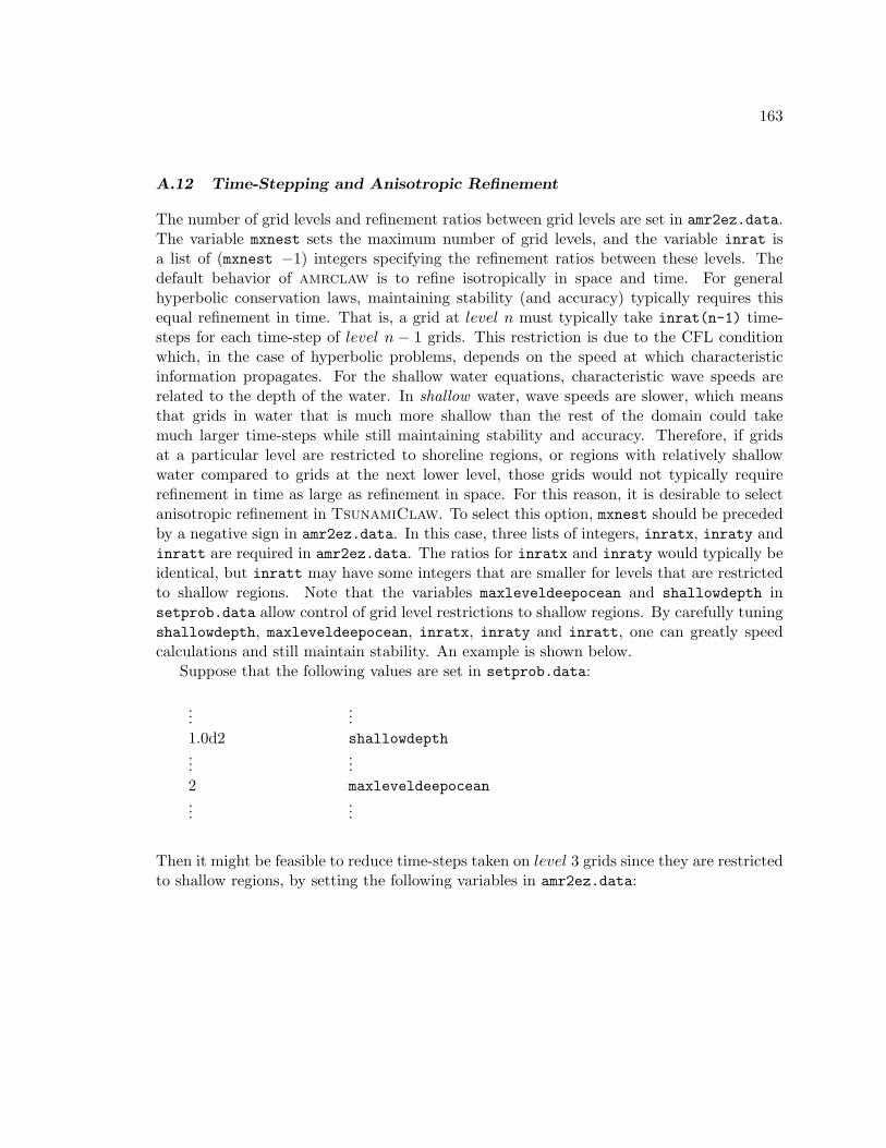
163

A.12 Time-Stepping and Anisotropic Refinement

The number of grid levels and refinement ratios between grid levels are set in amr2ez.data.The variable mxnest sets the maximum number of grid levels, and the variable inrat isa list of (mxnest −1) integers specifying the refinement ratios between these levels. Thedefault behavior of amrclaw is to refine isotropically in space and time. For generalhyperbolic conservation laws, maintaining stability (and accuracy) typically requires thisequal refinement in time. That is, a grid at level n must typically take inrat(n-1) time-steps for each time-step of level n − 1 grids. This restriction is due to the CFL conditionwhich, in the case of hyperbolic problems, depends on the speed at which characteristicinformation propagates. For the shallow water equations, characteristic wave speeds arerelated to the depth of the water. In shallow water, wave speeds are slower, which meansthat grids in water that is much more shallow than the rest of the domain could takemuch larger time-steps while still maintaining stability and accuracy. Therefore, if gridsat a particular level are restricted to shoreline regions, or regions with relatively shallowwater compared to grids at the next lower level, those grids would not typically requirerefinement in time as large as refinement in space. For this reason, it is desirable to selectanisotropic refinement in TsunamiClaw. To select this option, mxnest should be precededby a negative sign in amr2ez.data. In this case, three lists of integers, inratx, inraty andinratt are required in amr2ez.data. The ratios for inratx and inraty would typically beidentical, but inratt may have some integers that are smaller for levels that are restrictedto shallow regions. Note that the variables maxleveldeepocean and shallowdepth insetprob.data allow control of grid level restrictions to shallow regions. By carefully tuningshallowdepth, maxleveldeepocean, inratx, inraty and inratt, one can greatly speedcalculations and still maintain stability. An example is shown below.

Suppose that the following values are set in setprob.data:

......

1.0d2 shallowdepth...

...2 maxleveldeepocean...

...

Then it might be feasible to reduce time-steps taken on level 3 grids since they are restrictedto shallow regions, by setting the following variables in amr2ez.data:

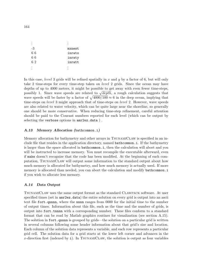
164

......

-3 mxnest6 6 inratx6 6 inraty6 2 inratt...

...

In this case, level 3 grids will be refined spatially in x and y by a factor of 6, but will onlytake 2 time-steps for every time-step taken on level 2 grids. Since the ocean may havedepths of up to 4000 meters, it might be possible to get away with even fewer time-steps,possibly 1. Since wave speeds are related to

√depth, a rough calculation suggests that

wave speeds will be faster by a factor of√

4000/100 ≈ 6 in the deep ocean, implying thattime-steps on level 3 might approach that of time-steps on level 2. However, wave speedsare also related to water velocity, which can be quite large near the shoreline, so generallyone should be more conservative. When reducing time-step refinement, careful attentionshould be paid to the Courant numbers reported for each level (which can be output byselecting the verbose options in amr2ez.data ) .

A.13 Memory Allocation (bathcommon.i)

Memory allocation for bathymetry and other arrays in TsunamiClaw is specified in an in-clude file that resides in the application directory, named bathcommon.i. If the bathymetryis larger than the space allocated in bathcommon.i, then the calculation will abort and youwill be instructed to increase memory. You must recompile the executable afterward, evenif make doesn’t recognize that the code has been modified. At the beginning of each com-putation, TsunamiClaw will output some information to the standard output about howmuch memory is allocated for bathymetry, and how much memory is actually used. If morememory is allocated than needed, you can abort the calculation and modify bathcommon.iif you wish to allocate less memory.

A.14 Data Output

TsunamiClaw uses the same output format as the standard Clawpack software. At userspecified times (set in amr2ez.data) the entire solution on every grid is output into an asciitext file fort.qnnnn, where the nnnn ranges from 0000 for the initial time to the numberof output times. Information about this file, such as the time and the number of grids, isoutput into fort.tnnnn with a corresponding number. These files conform to a standardformat that can be read by Matlab graphics routines for visualization (see section A.15).The solution in fort.qnnnn is grouped by grids—the solution on a particular grid is writtenin several columns following some header information about that grid’s size and location.Each column of the solution data represents a variable, and each row represents a particulargrid cell. The solution data for a grid starts at the lower left corner and advances in thex-direction first (indexed by i). In TsunamiClaw, the solution is output as four variables

165

in four columns: q(i,j,1) is the water depth, q(i,j,2) and q(i,j,3) are the momenta(depth times water velocity) in the x and y directions respectively, and q(i,j,4) is thesurface elevation, where 0 is mean sea level. Note that having the surface elevation and thewater depth allows determination of the bathymetry in a grid cell, since depth subtractedfrom surface elevation gives the elevation of the bathymetry or topography. Also, sinceTsunamiClaw solves the shallow water equations in their physically relevant conservativeform in order to allow convergence to bores, momenta are output rather than the morecommon variable of water velocity. Velocity can be recovered by dividing the momentumby depth. Some care should be exercised when doing this, since velocities at vanishingdepths may not be accurate, and division by zero for dry cells should obviously be avoided.

When using the latitude-longitude option to specify the computational domain, all out-put quantities are in units of meters and seconds. Therefore, in a particular grid cell,the momenta output in the solution are in the locally orthogonal longitude and latitudedirections, and given in meters squared per second.

A.15 Matlab Graphics and Output Visualization

TsunamiClaw comes with a set of Matlab plotting routines,.m files, in the directory$TSUNAMICLAW/matlab,

as well as a few routines in the example application directory. These routines are a mixof the standard Clawpack matlab plotting routines as well as several specialized routinesfor plotting with TsunamiClaw. If you use Clawpack software for other applications,then the $TSUNAMICLAW/matlab directory must be higher on your Matlab path than thestandard Clawpack Matlab routines, since some modified routines share the same name.(Much like Unix itself, which uses the PATH variable to specify its directory search path,Matlab uses the variable, MATLABPATH when run under Unix, which can also be set in yourlogin scripts.)

TsunamiClaw uses the Clawpack Matlab script plotclaw2.m as the main plottingroutine. Run plotclaw2 from the application directory (the file for the routine resides in theTsunamiClaw Matlab library). A number of plotting options are specified in setplot2.m,which resides in the application directory (see Clawpack documentation for descriptionsand examples). plotclaw2 calls setplot2 if you select yes when queried from the Mat-lab prompt. For some specialized TsunamiClaw plotting features, set PlotType=5 insetplot2.m. This creates a colored surface plot of the water surface and land, using somecolormaps provided in $TSUNAMICLAW/matlab. Waves are shaded from red at the peaks todark blue at the troughs. The default view is directly overhead, but note that these surfaceplots can be rotated and zoomed, either manually or by adjusting Matlab’s view properties.Specific user issued plotting features, such as axis labeling, axis limits, color axis propertiesfor the wave shading, or other options, can be specified in afterframe.m. The standardClawpack documentation provides a full explanation of how to use the Matlab plottingfeatures.

166

A.16 Acknowledgements

TsunamiClaw is an extension of the existing Clawpack software, including Amrclawadaptive mesh refinement routines and Matlab plotting routines. The two-dimensionalClawpack routines were written by

Randall J. LeVeque

University of Washington.

The adaptive mesh refinement algorithms were written by

Marsha Berger

Courant Institute, NYU.

Many of the Matlab plotting routines were written by

Donna Calhoun

CEA, Saclay France.

Numerous other people have contributed to Clawpack and Amrclaw in a variety of ways.Development of this software has been supported by grants from the NSF and the DOE.

A.17 Usage Restrictions

This software is made available for research and instructional use only. You may copyand use this software for these non-commercial purposes at no charge. For all other uses(including distribution of modified versions), please contact the authors. Since Tsunami-Claw is an extension of Clawpack, all of the usage restrictions and copyright notices forClawpack apply to TsunamiClaw.

This software is made available “as is,” without any assurance that it will work for yourpurposes. The software may have defects and is to be used at your own risk.

167

VITA

David L. George was born in San Francisco on February 20th, 1973. He earned Bachelor’sdegrees in Anthropology, Biology and Physics from the University of California, SantaBarbara. He received an M.S. in Applied Mathematics in 2004 and a Ph.D. in AppliedMathematics in 2006 from the University of Washington, Seattle.