FINITE VOLUME SIMULATION OF A FLOW OVER A NACA 0012 USING JAMESON, MacCORMACK, SHU AND TVD ESQUEMES

Oscar Arias a, Oscar Falcinelli b, Nide Fico Jr.a and Sergio Elaskar b,c

aInstituto Tecnológico de Aeronáutica, Brasil e-mail: nide@ita.br

bUniversidad Nacional de Córdoba. cCONICET, Argentina

Keywords: Finite volume, Jameson, MacCormack, Shu, TVD, NACA0012.

Abstract. In this paper is presented the results obtained by means numerical simulations of the flow over the NACA 0012 airfoil at different Mach numbers using two codes: one developed at Instituto Tecnológico de Aeronáutica of Brazil (ITA); the second developed at the Departamento de Aeronáutica de la Universidad Nacional de Córdoba (UNC). The computer code developed at ITA works with a boundary-fitted structured-grid context; and it solves the equations by a finite-volume technique, using three different time-marching schemes. The Euler flow was modeled as well as a Reynolds-averaged Navier Stokes formulation was calculated. Two Euler cases were done using the Jameson, MacCormack and the Shu schemes to advance in time. The computer code developed at the UNC uses a Total Variation Diminishing (TVD) scheme implemented in a non structured finite volume formulation for solving the 3D Euler equations is presented. Finally the pressure coefficient distribution along the airfoil chord and the contours of the flow properties were compared with other data available in literature.

1 INTRODUCTION

The numerical simulations comparison of the flow around the NACA 0012 airfoil at different Mach numbers using two codes are presented in this paper. The first code was developed at Instituto Tecnológico de Aeronáutica - ITA and the second software was developed at the Universidad Nacional de Córdoba - UNC.

Both computational codes implement a finite volume method to solve the Euler equations. The ITA code works on two-dimensional structured grid and it posses the capacity to work with three different schemes: (i) the Jameson scheme (Jameson et al, 1981) using a five stage Runge-Kutta time integration; (ii) the MacCormack scheme (MacCormack, 1984), based upon the predictor and corrector strategy to advance in time; (iii) and finally the Shu scheme (Yee, 1997), which uses a variation of the Jameson time integration, in order to better capture of shock waves. The UNC code works on three-dimensional unstructured grid and it implements three different numerical schemes: (i) the first order flux vector-splitting, (ii) the Harten-Yee TVD scheme (Harten, 1983; Yee, Warming and Harten, 1985), (iii) the improved Harten-Yee TVD techniques developed at the UNC (Falcinelli et al, 2007).

Furthermore, the computational effort, and total CPU time, related to the finite-volume schemes implemented is compared. The flow over the NACA 0012 at transonic and supersonic velocities was solving to calculate the general characteristics of each scheme.

2 DESCRIPTION OF THE ITA CODE

The description of the utilized schemes and the boundary conditions is presented in this section. This code was developed to solve aerodynamics flows.

2.1 Jameson scheme

The method developed by Antony Jameson and coworkers (Ortega, 1995; Pulliam, 1986) incorporates efficient stability characteristics and high compatibility to multigrid simulations. It applies a five-stage Runge-Kutta to advance the solution in time. The method is fourth-order accurate in time and second-order in space. The fluxes across the grid-cell surface are calculated by averaging the flow properties on both sides, giving rise to a central-discretization scheme. Therefore, it is intrinsically a central difference approximation in space. As a consequence, it requires the use of additional numerical dissipation terms in order to guarantee stability. In this case a non-linear artificial viscosity is used (Jameson et al., 1981).

To advance the solution in time Jameson suggested a five-stage Runge-Kutta integration scheme. The numerical dissipative terms are evaluated just in the first two stages (Mavriplis, 1988). The non-linear numerical dissipation has a pressure sensor that is somewhat more complicated than the one used here (Ortega, 1995). Therefore, the author decided to calculate these dissipative fluxes in all the Runge-Kutta stages to improve the stability. Thus, adding the numerical dissipation operator, one gets:

( ) ( ),, ,

,

1 0i je i j i j

i j

dQT Q Da Q

dt V⎡ ⎤+ − =⎣ ⎦ ,

where ( ),i jDa Q denotes the artificial viscosity. Let the superscript n denote the time level. Thus, 1n + represents the next time level after

a time increment equal to tΔ . To advance the calculation towards the steady state solution,

(1)

one writes:

( )0 nQ Q= ,

( ) ( ) ( )( ) ( )( )1 0 0 01

,

,ei j

tQ Q T Q Da QV

α Δ ⎡ ⎤= − −⎣ ⎦

( ) ( ) ( )( ) ( )( )2 0 1 12

,

,ei j

tQ Q T Q Da QV

α Δ ⎡ ⎤= − −⎣ ⎦

( ) ( ) ( )( ) ( )( )3 0 2 23

,

,ei j

tQ Q T Q Da QV

α Δ ⎡ ⎤= − −⎣ ⎦

( ) ( ) ( )( ) ( )( )4 0 3 34

,

,ei j

tQ Q T Q Da QV

α Δ ⎡ ⎤= − −⎣ ⎦

( ) ( ) ( )( ) ( )( )5 0 4 45

,

,ei j

tQ Q T Q Da QV

α Δ ⎡ ⎤= − −⎣ ⎦

( )51nQ Q+ = .

where the subscripts i,j in the Q vector where neglected for simplicity. The standard values for the α coefficients, used in the present work, are:

114

α = , 216

α = , 338

α = , 412

α = and 5 1α = .

2.2 MacCormack scheme

The explicit MacCormack algorithm (MacCormack, 1984) uses two steps to advance in time, one is the predictor and the other is the corrector. It is a second-order-accurate in both space and time. In the predictor step the flux vector at a certain face is calculated using the properties at the forward cell, whereas in the corrector step the properties values to be used are the ones relative to the backward cell. The discrete approximation of all the fluxes crossing the surface of the control volume for the predictor step is:

( ) ,21,,

21,1,,

21,,

21,1,

1

⎥⎥⎦

⎤

⎢⎢⎣

⎡⎟⎟⎠

⎞⎜⎜⎝

⎛⋅−⎟⎟

⎠

⎞⎜⎜⎝

⎛⋅+⎟⎟

⎠

⎞⎜⎜⎝

⎛⋅−⎟⎟

⎠

⎞⎜⎜⎝

⎛⋅=

−++

−++

+

jijijijijijijijijinp SPSPSPSPQT

and for the corrector it is:

( ) .21,

11,

21,

1,,

21

1,1,

21

1,,

1

⎥⎥⎦

⎤

⎢⎢⎣

⎡⎟⎟⎠

⎞⎜⎜⎝

⎛⋅−⎟⎟

⎠

⎞⎜⎜⎝

⎛⋅+⎟⎟

⎠

⎞⎜⎜⎝

⎛⋅−⎟⎟

⎠

⎞⎜⎜⎝

⎛⋅=

−

+−

+

+

−

+−

+

++

ji

njiji

njiji

njiji

njiji

nc SPSPSPSPQT

(2)

(3)

(4)

Considering the forward and backward discretization the scheme is as follows.

Predictor:

( ) ( ) ( )( ) ( )( )1 0 0 0

,

,pi j

tQ Q T Q Da QVΔ ⎡ ⎤= − −⎣ ⎦

Corrector:

( ) ( ) ( )( ) ( )( )2 0 1 1

,

,ci j

tQ Q T Q Da QVΔ ⎡ ⎤= − −⎣ ⎦

Update:

( ) ( ) ( )1 1 212

nQ Q Q+ ⎡ ⎤= +⎣ ⎦ .

The explicit MacCormack scheme, even though it is an upwind method, does not implicitly introduce a sufficient amount of artificial dissipation. Thus, it is necessary to explicitly add it. Without these terms the code diverges.

2.3 Shu scheme

Another procedure to advance the solution in time, utilized in this work, is that proposed by Shu (Shu, 1989) and explained by Yee (Yee, 1997). The resultant numeric method has good shock wave capturing characteristics. It uses a variant of the Runge-Kutta integration that needs only three steps:

( ) ( ) ( )( ) ( )( )1 0 0 0

,

,ei j

tQ Q T Q Da QVΔ ⎡ ⎤= − −⎣ ⎦

( ) ( ) ( ) ( )( ) ( )( )2 0 1 1 1

,

3 1 1 ,4 4 4 e

i j

tQ Q Q T Q Da QVΔ ⎡ ⎤= + − −⎣ ⎦

( ) ( ) ( ) ( )( ) ( )( )1 0 2 2 2

,

1 2 23 3 3

ne

i j

tQ Q Q T Q Da QV

+ Δ ⎡ ⎤= + − −⎣ ⎦ .

2.4 Boundary conditions

The types of boundary conditions used for this case are shown in Figure 1. The wall, far field and periodic boundary conditions are described next:

o Wall Boundary condition: In the Euler case the non-penetrability condition is used, forcing the flow to be tangent to a solid surface, see Figure 2.

(6)

(5)

(7)

(8)

Figure 1: Boundary Conditions for an O-grid.

Figure 2: Velocity Vectors next to a Solid Surface for Euler Formulation.

Thus, according to Figure 2, the velocity components 0U and 0V in the x and y direction, respectively, for the ghost volume must be

( )2 20 1 y x 1 x yU U n n 2V n n= − − ,

( )2 20 1 x y 1 x yV V n n 2U n n= − − ,

where the unit vector components in the x- and y-direction, nx and ny, are

(10)

(9)

( ), /i j 1 2xx

Sn

d−= ,

( ), /i j 1 2yy

Sn

d−= ,

and

( ) ( )/

, / , /

1 222x yi j 1 2 i j 1 2

d S S− −

⎡ ⎤= +⎢ ⎥⎣ ⎦

is the magnitude of the surface vector. o Far field boundary condition: The idea is to attribute free-stream values to all the flow

properties at the external boundary. It is important to point out that non-reflective boundary conditions were not implemented

o Periodic boundary condition: this could be considered as a different type of symmetry condition. The idea is to set the flux of all variables leaving the periodic outlet boundary equal to the flux entering the periodic inlet boundary. Therefore, for any property φ of the flow on a O-grid, this condition is established as

max

max

max

max

i i 1

i 1 i 2

i 0 i 1

i 1 i 2

φ φ

φ φ

φ φ

φ φ

=

+ =

= −

=− −

=

=

=

=

Finally it is important to point out that the initial conditions, necessary to start the iteration process, were the free-stream values over the entire computational domain.

2.5 Validation test cases for the ITA code

To validate the correct behavior of the ITA code are carried out numerical simulations of the inviscid flows over the NACA 0012 airfoil. The results are compared with other results available in the literature. The numerical simulations were carried out on a Dell computer Latitude D600, Pentium V, with a 1700-Mhz processor and 512 MB of RAM. The numerical solution convergence was checked calculating the maximum density variation over the entire computational domain. If it was smaller than 910− , the program stops.

For comparative purposes, the schemes of Jameson, MacCormack and Shu have been used to solve transonic and supersonic flow over the NACA 0012 airfoil. For the transonic case the Mach number is 0.8M∞ = and 1.25α = . For the supersonic case the Mach number is 1.2 at zero angle of attack. All numerical simulations were done with a boundary-fitted structured grid using 189 x 53 elements in the i and j direction respectively. The pressure coefficient along the airfoil and the convergence rate were evaluated. The schemes were run with the maximum CFL number possible. Thus, the CFL number was equal to 1.7, for the Jameson method, 0.4 for MacCormack, and 0.6 for the Shu formulation. The non-linear artificial viscosity coefficients for both cases were 2K = 2 and 4K = 0.035.

(11)

(12)

2.6 Mach 0.8, Alpha 1.25

All The pressure coefficients of the different schemes are shown in Figure 3. All the results presented by this code looks similar as that provided by Pulliam (Pulliam, 1986), using a finite difference method and Jameson-Mavriplis using a regular triangular mesh.

Figure 3: Pressure Coefficient Comparison for Jameson, McCormack and Shu Schemes.

The suction peak at the upper surface was found to be approximated -1.1 for our present simulations comparing with the Pulliam solution. However, for all the results, including that one of Pullian, the upper shock wave was shifted towards the leading edge when compared with the Jameson-Mavriplis solution, as reported by Wenneker (Wenneker, 2002) on his doctoral thesis. This could happens because of the entropy generation at the leading edge, which creates a ‘numerical boundary layer’, causing losses (close to the airfoil) that are visible in the constant Mach lines, see Figure 4. The weak shock wave, at the lower part of the airfoil, is particularly hard to capture, but all the schemes did it good. However, there was a difference in the lower shock when compared with Pulliam. Jameson predicts the shock wake formation before Pullian, while Shu is capture the shock almost at the same position of Pulliam. MacCormack predicts a stronger aft positioned shock. This difference may be related to two possible reasons: one is the AV coefficients combined with the type of grid used by Pulliam, and the other is the use by Pullian of upwind differencing in supersonic regions, as suggested by Steger (Steger, 1978), producing better shock capturing capabilities. However, it should be pointed out that the Cp minimum value, around -0.68, was the same for all the schemes.

Examining the convergence history, in Figure 5, the differences start to show up. During the first 1000 iterations, the Jameson formulation showed a highly oscillatory behavior, but after 1400, these oscillations were periodic until the convergence criterion was achieved. The MacCormack implementation had an initial behavior similar to that of Jameson. However, it took more than three times more iterations (16,120) to attain the convergence criterion. For Shu scheme, the first 1,000 iterations showed a significant residue drop. Unfortunately, as the computation continued, the density variation raised again. Just over 7000 time steps the residue looked stable in its way to convergence, but the very tight convergence criterion was reached after 23,506 iterations, a number higher than the other schemes.

Figure 4: Mach contours using the Jameson scheme

For a better understanding of these results, the computational effort, ξ, was calculated.

According to Beam and Warming (Beam and Warming, 1978).

Number of time stepsCP

I Jξ =

⋅ ⋅

where I and J are the number of grid points along each direction, CP is the computational time in seconds, and the number of steps is the total number of iterations. The results were putted together in Table I:

The MacCormack method generated 62.70% less computational effort than the Jameson method. This was because a predictor-corrector procedure was used to advance the solution in time. Thus, there were only two steps per iteration. The Shu scheme demanded 42.13% less effort than Jameson, because it used a three-step Runge-Kutta. This is a variation from the original five step Runge-Kutta formulation. In regard to the CPU time process, a more realistic figure of merit, Jameson was 24.9% faster than MacCormack, and Shu took almost three times longer than Jameson.

(13)

Y

X

Figure 5: Comparison of density variation histories.

CFLmax Comp. Time Cp (sec) Iterations Comp. Effort

ξ (sec)

Jameson 1.7 1380 4.511 3.05 x 5-10

MacCormack 0.4 1839 16.120 1.13 x 5-10

Shu 0.6 4161 23.506 1.76 x 5-10

Table I: Computational effort for different schemes.

The main idea of using the Shu variant was to improve the results, particularly in respect to a better shock wave resolution. Although the general pressure distribution with this technique is almost the same as the others, there is an improvement in the lower shock wave position. This scheme shows the closets results to the distribution presented by Pulliam. No other improvement was obtained by the present author. The MacCormack scheme, although it took 19.8% more time than the Jameson scheme, showed a considerable lower computational effort. This suggests that it maybe adequate for very fine mesh, like the ones used for viscous simulations.

2.7 Mach 1.2, Alpha 0

A supersonic flow, 1.2M∞ = , over the NACA 0012, at zero angle of attack was simulated using the same 189 x 53 grid of the transonic calculation. For this case the CFL values were the same as the previous case for all the schemes.

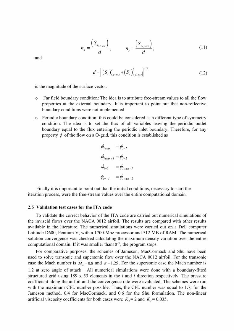
In figure 6 the results are compared with those presented by Yoshihara & Sacher (Yoshihara and Sacher, 1985) and Wenneker (Wenneker, 2002). The circles correspond to the Yoshihara solution. The delta symbols indicate the results presented by Wenneker using an unstructured grid with 31,144 cells. The Cp distribution found using the three different schemes is in very good agreement with the literature, except for a very mild asymmetry, almost imperceptible, located close to the leading edge.

Figure 6: Pressure Coefficient Comparison for 1.2M ∞ = and 0.0α = .

Comparison of the constant Mach lines of the Jameson scheme with the Wenneker result is shown in Figure 7. The result obtained by the present code was similar to that presented by that researcher. However, the bow shock did appear to be thicker. Further, Yoshihara and Sacher found the shock position to be at x/c = - 0.42 from the leading edge.

(a) (b)

(c)

Figure 7: Mach Isolines Comparison from (a) Wenneker and (b) ITA code. (c) Mach Contours.

The shock position data is condensing in table II. Wenneker obtains -0.43 while the Jameson calculation gets -0.4194, a value almost exactly to that of Yoshihara. The MacCormack and Shu formulations provided both a higher error, of an order of 5 %.

This could be produce not only due to the differences in the schemes, it could also be due to the fact that reflective boundary conditions are not implemented here, and, as the simulation advance in time, there is more possibility to contaminated the airfoil with returning disturbances form the far field boundary. This could be possible especially for the schemes that take more time to converge.

Yoshihara & Sacher Wenneker Jameson MacCormack Shu

Shock Position -0.42 -0.43 -0.4194 -0.3958 -0.40

Error (%) ------- 2.38 0.14 5.7 4.76

Table II: Shock wave position.

Figure 8: Comparison of density variation histories.

CFLmax Comp. Time Cp (sec) Iterations Comp. Effort

ξ (sec)

Jameson 1.7 606 2.111 2.86 x 5-10

MacCormack 0.4 926 7.415 1.24 x 5-10

Shu 0.6 3240 13.637 2.37 x 5-10

Table III: Computational effort for different schemes.

The density residue is shown in Figure 8 and the computational effort is shown in table III. It is clear that again the MacCormack scheme has the lower computational effort, 56% lower than Jameson, and Shu was close to Jameson, showing 17% less effort.

3 DESCRIPTION OF THE UNC CODE

The three-dimensional Euler equations can be written as:

U F 0t

∂+ ∇ ⋅ =

∂ (14)

where U is the vector of conservative variables, and F is the 3D vectorial flow.

The temporal change of the conservative variables can be written as:

1 *

10

nfacesn n

j j jj

tU U F n AVol

+

=

Δ= − ⋅ • ⋅ =∑ (15)

The numerical flux projection in the direction normal to the face “i”, *i iF • n = *

i+1/2f , is calculated using the TVD scheme proposed for Harten (Yee, 1997; Harten, 1983) and modified by Yee (Yee, Warming and Harten, 1985). Although this method was originally developed for finite differences techniques, it has been extended successfully for finite volume formulations similar to the one used in this work (Udrea, 1999).

The Eq. 15 implies the use of a locally aligned system of coordinates whose unit vector i coincides with the normal to the face of the cell, and the unit vectors j and k are tangential directions. Since the local Riemann problem is solved with rotated data, the eigensystem is calculated in the locally aligned coordinate frame. The numerical flux can then, be expressed as:

____

* 11/ 2 1/ 2 1/ 2

12 2

m mi ii i i

m

f ff r+

+ + ++

= + ⋅ Φ ⋅∑ (16)

where fi and fi+1 are the physical fluxes normal to the face in each cells, ____

1/ 2m

ir + is the m-th right eigenvector, and 1/ 2

mi+Φ is, in the original Harten-Yee scheme, defined as:

1/ 2 1 1/ 2 1/ 2 1/ 2m m m m m mi i i i i ig g+ + + + +Φ = + − λ + γ ⋅ α (17)

being:

( )1/ 2 1/ 2 1/ 2 1/ 2max 0,min ,2

m m m m mi i i i i

Sg S+ + − −⎡ ⎤= ⋅ λ ⋅ α ⋅ λ ⋅ α⎣ ⎦ (18)

( )1/ 2miS sign += λ ;

11/ 2

1/ 21/ 2

1/ 2

0

0 0

m mmi iim

imi

mi

g g si

si

++

+

+

+

⎧ −α ≠⎪ α⎪

γ = ⎨⎪ α =⎪⎩

(19)

where 1/ 2mi+α is the jump of the conserved variables across the interfaces between cells “i” and

“i+1”, and 1/ 2mi−λ is the m-th eigenvalue of the Jacobian matrix.

The limiter function given in Eq. (18) is known as minmod (Sweeby, 1984; Leveque, 1992). The minmod selects the minimum possible value, so that the scheme is TVD. The other end is the limiter function “superbee” (Hirsch, 1992) that ponders the contribution of the high order flux. The implementation of this function leads to an excessively compressive scheme which it is not very robust for general practical applications.

In the numerical solution of the three-dimensional Euler equations five wave families appear. If the five wave families are enumerated in correspondence with their speed, being one the slowest and five the faster, it can be demonstrated that for waves of the families two to four, the characteristic velocities at both sides of the discontinuity are the same and equal to the velocity discontinuity (Hirsch, 1992; Toro, 1999). This property makes very difficult to solve theses waves accurately, unless they are solved diffusely.

In this work, it is explored the possibility of implementing different limiter functions for different wave families. The objective is to improve the numerical resolution of the discontinuities associated with the families two to four using compressive limiter functions (superbee), and without losing robustness due mainly to the use of diffusive limiter functions (minmod) for the wave families one and five.

To introduce in the numerical fluxes calculations the limiter function superbee the Eq. (18) is replaced by the following expression:

( ) ( )

1/ 2 1/ 2

1/ 2 1/ 2 1/ 2 1/ 2

0 if 0

1max 0,min 2 ,1 ,min ,2 if 02

m mi i

mi

m m m mi i i i

g

r r

+ −

− − + −

⎧⎪ α ⋅α <⎪

= ⎨⎪⎪ ⋅ ⋅ ⋅ λ ⋅α α ⋅α ≥⎡ ⎤⎣ ⎦⎩

(20)

being: 1/ 2 1/ 2 1/ 2 1/ 2/m m m mi i i ir + + − −= λ ⋅α λ ⋅α .

To improve the overall scheme robustness, the implementation of different limiter functions is carried out only in those cells interfaces where the greater relative intensities of the discontinuities in central waves are registered, and using the conventional Harten-Yee TVD scheme in all other cases (Falcinelli, Elaskar and Tamagno, 2007).

3.1 Boundary conditions

The treatment of the boundary conditions is carried out through the imaginary cells technique (Hirsch, 1992; Toro, 1999). Five different types of boundaries are considered: 1 – Subsonic inlet, 2 - Supersonic inlet, 3 – Subsonic exit, 4 - Supersonic exit, 5 - Non penetration (solid boundary and symmetry).

3.2 Validation test cases for the UNC code

In order to verify the accuracy and robustness of the proposed scheme two test cases are simulated. The first one is the flow inside of a shock tube. This example is used to explore the capacity of the scheme which has been described, to model contact discontinuities; the flow does not have velocity regarding the contact discontinuity (discontinuity in waves of the family 2). The second test is the simulation of a slip layer between two flows with different velocities and densities, and equal pressures. This test was chosen to study the capacity of the scheme to solve flows in which the discontinuity is in the velocity tangent to a given interface (discontinuity in waves of the families 3 and 4). The numerical simulations of the UNC code were realized on notebook PENTIUM IV de 2.60GHz con 248MB de RAM

3.3 Flow inside a Sock tube

The shock tube has a rectangular section of 4cm x 4cm and a length of 2m; the gas is air. The driver section is filled with atmospheric initial conditions. The pressure in the driven section is 0.1 atmospheres and possesses the same temperature than the driver. The analytical solution is given by a three waves system, a shock wave that advances toward the right at 543.4m/s, a contact discontinuity that also moves toward the right at 277.6m/s and an expansion fan whose head wave travels to the left at 4.9 m/s and the tail wave traveling at 338.1 m/s leftward also18.

The computational mesh is obtained by means of a “generating cell” built up by 6 tetrahedrons that form a cube of 1cm side length. The cube is repeated up to complete an arrangement of 4x4x200.

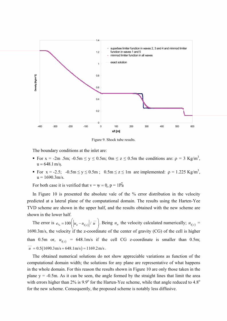
Figure 9 shows the density as a function of (x/t). In this figure are compared: the analytical solution, the results obtained applying the new TVD scheme and those obtained with the conventional Harten-Yee TVD scheme. It can be appreciated that capture of the contact discontinuity has been improved notably. Furthermore, the absence of oscillations next to discontinuities can clearly be seen, as well as the accuracy achieved with the speed of the waves.

3.4 Slip surface

The second test case is an air layer with a density of 1.225Kg/m3, a velocity of 1690.3m/s and a pressure of 100000Pa, that flows over another layer with a density of 3Kg/m3, a velocity of 648.1m/s and a pressure of 100000Pa. The analytical solution predicts the slip of a flow on another without interferences. However, due to the numerical viscosity, the computed solution produces an apparent mixture zone that gets wider downstream the end of the splitter plane. The spreading of such unphysical mixing region quantifies the lack of accuracy of the numerical method.

In this second case, the mesh has 57.790 tetrahedrons and 11.503 nodes. The control volume where the flow develops is 5m long, 1m high and 1m wide. The non-structured mesh does not have any bias plane that may influence the location of the slip discontinuity.

0

0.2

0.4

0.6

0.8

1

1.2

1.4

-400 -300 -200 -100 0 100 200 300 400 500 600

x/t [m]

Dens

ity [K

g/m

^3]

superbee limiter function in waves 2, 3 and 4 and minmod limiterfunction in waves 1 and 5minmod limiter function in all waves

exact solution

Figure 9. Shock tube results. The boundary conditions at the inlet are:

For x = -2m .5m; -0.5m ≤ y ≤ 0.5m; 0m ≤ z ≤ 0.5m the conditions are: ρ = 3 Kg/m3, u = 648.1m/s.

For x = -2.5; -0.5m ≤ y ≤ 0.5m ; 0.5m ≤ z ≤ 1m are implemented: ρ = 1.225 Kg/m3, u = 1690.3m/s.

For both case it is verified that v = w = 0 , p = 1Pa

In Figure 10 is presented the absolute vale of the % error distribution in the velocity predicted at a lateral plane of the computational domain. The results using the Harten-Yee TVD scheme are shown in the upper half, and the results obtained with the new scheme are shown in the lower half.

The error is ( )

___

% 100 /n t ze u u u⎛ ⎞= −⎜ ⎟

⎝ ⎠. Being nu the velocity calculated numerically; ( )t zu =

1690.3m/s, the velocity if the z-coordinate of the center of gravity (CG) of the cell is higher

than 0.5m or, ( )t zu = 648.1m/s if the cell CG z-coordinate is smaller than 0.5m;

( )___

0.5 1690.3m/s 648.1m/s 1169.2m/su = + = .

The obtained numerical solutions do not show appreciable variations as function of the computational domain width; the solutions for any plane are representative of what happens in the whole domain. For this reason the results shown in Figure 10 are only those taken in the plane y = -0.5m. As it can be seen, the angle formed by the straight lines that limit the area with errors higher than 2% is 9.9o for the Harten-Yee scheme, while that angle reduced to 4.8o for the new scheme. Consequently, the proposed scheme is notably less diffusive.

Figure 10. Slip surface results. Error: white 0% 2%e≤ ≤ , green 2% 5%e≤ ≤ , yellow 5% 10%e≤ ≤ , light blue 10% 20%e≤ ≤ , red 20% e≤ .

4 CODES COMPARISON

In this section are presented the numerical results obtained by means of the ITA and UNC codes. The simulations carried out by the ITA code consider two dimensional flow and structured meshes. The numerical simulations obtained with the UNC code consider three dimensional flow and non-structured meshes; the used finite volumes are tetrahedrons with four nodes.

Four tests were realized: 1 – NACA 0012, M = 3, α = 0o

2 – NACA 0012, M = 7, α = 1.25o

3 – NACA 0012, M = 8, α = 1.25o

4 – NACA 0012, M = 1.2, α = 0o

To make comparable the results, the 3D meshes used for the UNC code and the 2D meshes implemented at the ITA code posse equal number the nodes over the airfoil.

For the UNC code, the numerical results were obtained using the conventional Harten-Yee TVD scheme.

Figures 11, 12 and 13 show that the ITA codes posses a better behaviour principally in transonic regime (M = 0.8). For this case the UNC predicts the shock wave formation with a 10% error. However, the UNC code reproduces with more accuracy the sharper form of the shock wave. For the supersonic flow (M = 1.2) both codes reproduce correctly the Cp distribution (see Figures 6 and 14).

The results obtained by UNC codes correspond to 3D simulations. It can be appreciated from Figures 11, 12, 13 and 14 that the scattering of the results at each x-station is very small compared with related local dynamic pressures.

-0.6

-0.4

-0.2

0

0.2

0.4

0.6

0.8

0 0.2 0.4 0.6 0.8 1

x/c

Cp

UNC code ITA code

Figure 11. Comparison for airfoil NACA 0012, M = 0.3, α = 0o

-1.2

-1

-0.8

-0.6

-0.4

-0.2

0

0.2

0.4

0.6

0.8

1

0 0.2 0.4 0.6 0.8 1

x/c

Cp

UNC code ITA code

Figure 12. Comparison for airfoil NACA 0012, M = 0.7, α = 1.25o

5. CONCLUSIONS

The main task was to simulate, using two codes, the invisid flow over the NACA 0012 airfoil considering different Mach numbers (M = 0.3; 0.7; 0.8; 1.2). The first code developed at ITA and the second at the UNC.

Both codes use finite volume to solve the Euler equations, however have different objectives, structures and techniques. The ITA code was developed to simulate subsonic and transonic aerodynamics flows; the UNC code posses the objective to simulate supersonic and hypersonic flows. The codes has been validate in function of their objectives.

The main conclusion is that the ITA code presents better behavior to predict the pressure distribution over the airfoil for subsonic and transonic flows. For supersonic flows (M = 1.2) the numerical results of the two codes were very good. However, the UNC captures more accurately the sharper form of the shock wave (M = 0.8). Theses conclusions are in concordance with the objectives for the both codes. The following step is to carry out comparison for high supersonic flows.

-1.5

-1

-0.5

0

0.5

1

1.5

0 0.2 0.4 0.6 0.8 1

UNC ITA

x/c

Cp

Figure 13. Comparison for airfoil NACA 0012, M = 0.8, α = 1.25o

Figure 14. Comparison for M = 1.2, α = 0o. Blue: Wenneker. Green: AGARD. Red: UNC code. Finally, the simulations with the ITA code revealed that the Jameson scheme, although

demanding more computational effort than the MacCormack’s, generated much better results at least for the NACA 0012 cases studied. Moreover, Jameson’s scheme allows for greater CFL numbers, which could, at least in part, compensate the larger number of iterations it needs to converge, as well as, the more computer intense calculations between time steps. Furthermore, it was not possible to run the MacCormack scheme without artificial viscosity terms, despite its upwind character.

REFERENCES

Beam, Richard; Warming, R. F. An implicit factored scheme for the compressible Navier- Stokes Equations. AIAA Journal, 16(4): 393-402, April, 1978.

Falcinelli Oscar, Elaskar Sergio and Tamagno José, Reducing the Numerical Viscosity in Non Structured Three-Dimensional Finite Volumes Computations. AIAA Journal of Spacecraft and Rockets, submitted, 2007.

Harten, A. High resolution schemes for hyperbolic conservation laws, Journal of Computational Physics, 49:250-257, 1983.

Hirsch, C., Numerical Computation of Internal and External Flows, Vol.2 Computational Methods for Inviscid and Viscous Flows, John Wiley & Sons Ltd., London, 1992.

Jameson, A.; Schimidt, W.; Turkel, E. Numerical solution of the Euler Equations by finite volume methods using runge-kutta time-stepping schemes. In Fluid And Plasma Dynamics Conference, 14., 1981, Palo Alto. Palo Alto: AIAA, 1981. Paper No.81-1259

Leveque, R. J., Numerical Methods for Conservation Law, Birkhäuser Verlag, Basel, 1992. MacCormack, R. W. An introduction and review of the basics of computational fluid

dynamics. Washington, DC: University of Washington, 1984. (Lectures notes) Mavriplis, D. J. Multigrid solution of the two-dimensional Euler equations on unstructured

triangular Meshes. AIAA Journal, 26(7): 824-831, 1988. Ortega, M. A. Apostila do curso de CFD. São José dos Campos: Instituto Tecnológico de

Aeronáutica, 1995. Pullian, Thomas. Artificial dissipation models for Euler equations. AIAA Journal, 24(12):

1931-1940, December, 1986. Shu, Chi-Wang. Efficient Implementation of Essentially Non-oscillatory Shock Capturing

Schemes II. Journal of Computational Physics, 83:32-78. 1989. Steger, J. L. Implicit finite difference simulation of flow about arbitrary geometries with

applications to airfoils. AIAA Journal, 16:679, July, 1978. Sweeby P.K., High Resolution Schemes Using Flux Limiters for Hyperbolic Conservation

Laws, SIAM Journal on Numerical Analysis, 21:995-1011, 1984. Toro, E. F., Riemann Solvers and Numerical Methods for Fluid Dynamics, Springer-Verlag,

Berlin, 1999. Udrea, B. An advanced implicit solver for MHD, PhD Thesis, University of Washington,

1999. Wenneker, Ivo. Computation of flows using unstructured staggered grids. 2002. Thesis. (PhD

Dissertation) - DELFT University of Technology, Delft, The Netherlands. Yee, H. C. Explicit and implicit multidimensional compact high-resolution shock capturing

methods formulation. Journal of Computational Physics, 131:216-232, 1997. Yee, H.C., Warming, R.F. and Harten, A., Implicit Total Variation Diminishing (TVD)

Schemes for Steady-State Calculations, Journal of Computational Physics, 57:327-360, 1985.

Yoshihara H., Sacher, P. Test cases for inviscid flow field methods. AGARDograph No. 211, AGARD, Neuilly-sur-Seine, France, 1985.