Embed Size (px)
Citation preview

FINITE WORD LENGTH EFFECTS IN DSP
PREPARED BY GUIDED BY Snehal Gor Dr. Srikanth T.

ABSTRACT
We know that computers store numbers not with infinite precision but rather in
some approximation that can be packed into a fixed number of bits or bytes, because of
which we are loosing some information. Our aim is to study the effect of loosing this
information on the response of digital filters. This effect we called Finite word length
effect.
There are number of effects of finite word length like overflow error in addition,
round off error in multiplication, effects of coefficient quantization, limit cycle, etc. This
paper talks about effects on response of IIR filters for the case of coefficient quantization.
Section 1 gives brief introduction to number system and shows why finite word
length effect occurs. Section 2 studies same phenomena from the view point of filters it
also includes results we have obtained.
We have studied effect of finite word length on the response of Butterworth low
pass IIR filter. Also we have studied effect of finite word length on the response of 4th
order IIR filter for direct form and parallel form realization. On the basis of results we
have concluded well known result that parallel form realization is better than direct form
realization.
2

1. INTRODUCTION
Computers store numbers not with infinite precision but rather in some
approximation that can be packed into a fixed number of bits or bytes. Almost all
computers allow the programmer a choice among several different such representations
or data types. Data types can differ in the number of bits utilized, but also in the more
fundamental respect of whether the stored number is represented in fixed-point or
floating-point format.
1.1 Fixed point representation
A number in fixed point representation is exact. Arithmetic between numbers in
fixed point representation is also exact, with the conditions that (i) the answer is not
outside the range of integers that can be represented, and (ii) that division is interpreted as
producing an integer result, throwing away any integer remainder. There are many
formats to represent fixed point numbers like, Sign-magnitude, One’s compliment and
Two’s compliment, etc.
A Real number can be represented with infinite precision in two’s complement
form as
∑∞
=
−+−=1
0 )(i
iim zbbXx
Where, Xm is an arbitrary scale factor and bi’s are either 0 or 1. The quantity b0 is referred
to as sign bit. If b0 = 0, then 0 ≤ x ≤ Xm and if b0 = 1, then Xm ≤ x < 0.
An arbitrary real number x would require an infinite number of bits for its exact
binary representation. If we use only a finite number of bits (B+1), then the
representation of above equation must be modified to
∑=
− =+−==B
iBm
iimB xXzbbXxQx
10 ˆ)(][ˆ
3

The resulting binary representation is quantized, so that the smallest difference
between numbers is
∆ = Xm2-B
The operation of quantizing number to (B + 1) bits can be implemented by
rounding or by truncation, but in either case quantization is a nonlinear memory less
operation. Figure 1.1 shows input - output relation for two’s complement rounding and
truncation, respectively, for the case of B = 2.
Figure 1.1 Nonlinear Relationship representing two’s complement (a) rounding and
(b) truncation for B = 2 [1]
In considering the effects of quantization, we often define quantization error as
e=QB[x] – x. For the case of two’s complement rounding, -∆/2 < e ≤ ∆/2, and for two’s
complement truncation, -∆ < e ≤ 0(Figure 1.2).
4

Figure 1.2 probability density function for quantization errors (a) Rounding (b)
Truncation. [1]
If a number is larger than Xm, a situation called overflow occurs. Figure 1.3 (a)
shows two’s complement quantizer, including the effect of regular two’s complement
arithmetic overflow. An alternative, which is called saturation overflow or clipping, is
shown in figure 1.3 (b). This method of handling overflow is generally implemented for
A/D conversion, and it sometimes is implemented in specialized DSP microprocessor for
addition of two’s complement numbers. With saturation overflow, the size of the error
does not increases abruptly when overflow occurs; however disadvantage of such
methods is that it voids the property of two’s complement-arithmetic that ‘If several
two’s-complement numbers whose sum would not overflow are added, then the result of
two’s-complement accumulation of these numbers is correct even though intermediate
sums might overflow”.
5

Figure 1.3 Two’s complement rounding (a) Natural Overflow (b) Saturation. [1]
1.2 Floating point representation
In floating-point representation (IEEE 754 standard), a number is represented
internally by a sign bit s, an exact integer exponent E, and an exact positive integer
mantissa M. Taken together these represent the number
fx Es .121 127 ∗∗−= −
where E is eight bit exponent (0 < E <255), s is sign bit ( 0 for positive and 1 for negative
) and f is 23 bit fraction )2
120( 23
23 −<< f . Floating point representations provide a
convenient means for maintaining wide dynamic range.
6

2. FINITE WORD LENGTH EFFECTS
Numerical quantization affects the implementation of linear time-invariant
discrete time system in several ways. Below we have given brief overview of some of
them.
• Parameter quantization in digital filters
In the realization of FIR and IIR filters hardware or in software on a general
purpose computer, the accuracy with which filter coefficients can be specified is limited
by word length of the computer. Since the coefficients used in implementing a given
filter are not exact, the poles and zeros of system function will be different from desired
poles and zeros. Consequently, we obtain a filter having a frequency response that is
different from the frequency response of the filter with unquantized coefficients. Also it
sometimes affects stability of filter.
• Round off noise in multiplication
As already explained when a signal is sampled or a calculation in the computer is
performed, the results must be placed in a register or memory location of fixed bit length.
Rounding the value to the required size introduces an error in the sampling or calculation
equal to the value of the lost bits, creating a nonlinear effect. Round off error is a
characteristic of computer hardware.
• Sampling/Digitization Error
There is another, different, kind of error that is a characteristic of the program or
algorithm used, independent of the hardware on which the program is executed. Many
numerical algorithms compute “discrete” approximations to some desired “continuous”
quantity. For example, an integral is evaluated numerically by computing a function at a
discrete set of points, rather than at “every” point. Or, a function may be evaluated by
7

summing a finite number of leading terms in its infinite series, rather than all infinity
terms. In cases like this, there is an adjustable parameter, e.g., the number of points or of
terms, such that the “true” answer is obtained only when that parameter goes to infinity.
Any practical calculation is done with a finite, but sufficiently large, choice of that
parameter. The difference between the true answer and the answer obtained in a practical
calculation is called the truncation error. Truncation error would persist even on a
hypothetical, “perfect” computer that had an infinitely accurate representation and no
round off error.
• Overflow in addition
Overflow in addition of two or more binary numbers occurs when the sum
exceeds the word size available in the digital implementation of the system.
• Limit cycles
Since quantization inherent in the finite precision arithmetic operations render the
system nonlinear, in recursive system these nonlinearities often cause periodic oscillation
to occur in the output, even when input sequence is zero or some nonzero value. Such an
oscillation in recursive systems are called limit cycles.
As explained in above paragraphs finite word length affects LTI system in many
ways. We have concentrated on effects due to coefficient quantization on filter response
and in that also on IIR filters. Later we have given brief overview of effects of coefficient
quantization in FIR system for the sack of completeness.
2.1 Effects of coefficient quantization in IIR system
When the parameters of a rational system function or corresponding difference
equation are quantized, the poles and zeros of the system move to the new position in the
z-plane, equivalently, the frequency response is perturbed from the original value.
8

The system function representation corresponding to both direct forms is
∑
∑
=
−
=
−
−= N
k
kk
M
k
kk
za
zbzH
1
0
1)(
The sets of coefficients ak and bk are ideal infinite-precision coefficients. If
we quantize these coefficients, we obtain the system function
∑
∑
=
−
=
−
−= N
k
kk
M
k
kk
za
zbzH
1
0
ˆ1
ˆ
)(ˆ
where âk = ak + ∆ak and bk = bk + ∆bk are the quantized coefficients that differ from
original coefficients by quantization by quantization error ∆ak and ∆bk.
Kaiser showed that if poles (or zeros) are tightly clustered it is possible that small
error in denominator (numerator) coefficient can cause large shifts of the poles and
(zeros) for direct form structure. Thus, if the poles (zeros) are tightly clustered,
corresponding narrow band pass filter or narrow-bandwidth low pass filter, then we can
express poles of the direct-form structure to be quite sensitive to quantization error in the
coefficients. Kaiser analysis also showed that the larger the number of clustered poles
(zeros), the greater is the sensitivity to quantization error.
The cascade and parallel form system function is consists of second order direct-
form systems. However, in both cases each pair of complex conjugate poles pair is
realized independently of all other poles. Thus, the error in a particular pole pair is
independent of its distance from the other poles of system function.
For the cascade form same arguments holds for the zeros, since they are realized
as independent second order factors. Thus cascade form is generally much less sensitive
to coefficient quantization than the equivalent direct-form realization.
9

∏+
=−−
−−
−−++
=2/)1(
12
21
1
22
110
1)(
N
k kk
kkk
zazazbzbbzH
The zeros of the parallel form structure are realized implicitly through combining
the quantized second order sections. Thus, particular zero is affected by quantization
error in the numerator and denominator coefficients of all the second order sections.
However for most practical filter the parallel form is also found to be much less sensitive
to coefficient quantization than the equivalent direct-form realization.
∑∑+
=−−
−−
=
−
−−+
+=2/)1(
12
21
1
110
0 1)(
N
k kk
kkNM
k
kk zaza
zeezCzH
In summery, because of the sensitivity to finite word length effect, the direct
forms are rarely used for implementing anything other than second - order structures.
Cascade and parallel structures are more often used.
2.1.1 What we did
Before jumping on to designing of filters and seeing finite word length effect let
us explain what we have did. Here we are not going to explain designing of filters or any
other filter designing fundamentals, one can refer any good book available for same[1][2].
But one should ask how we did quantization, so let us explain how we did quantization
and give some examples which show capability and limitation of our routine.
Our quantization routine is very simple and it basically performs following steps:
1) Take 32 bit floating point number between ranges 0 to 2.
2) Multiply it with 231 – 1 (if your numbers are between 0 to 1 then multiply it with
232 – 1) to get equivalent integer number stores it in 32 bit format
3) Shift above number required number of bits as per requirement to obtain N bits
representation of corresponding number (In a way make zero least significant
32 – N bits. So we have number which is still in 32 bits but least significant bits
removed).
4) Convert above number back into corresponding floating point number.
10
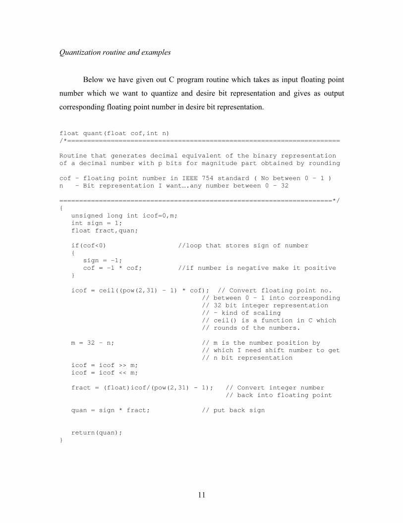
Quantization routine and examples
Below we have given out C program routine which takes as input floating point
number which we want to quantize and desire bit representation and gives as output
corresponding floating point number in desire bit representation.
float quant(float cof,int n) /*===================================================================== Routine that generates decimal equivalent of the binary representation of a decimal number with p bits for magnitude part obtained by rounding cof – floating point number in IEEE 754 standard ( No between 0 – 1 ) n - Bit representation I want….any number between 0 - 32 =====================================================================*/ unsigned long int icof=0,m; int sign = 1; float fract,quan; if(cof<0) //loop that stores sign of number sign = -1; cof = -1 * cof; //if number is negative make it positive
icof = ceil((pow(2,31) – 1) * cof); // Convert floating point no. // between 0 – 1 into corresponding // 32 bit integer representation // - kind of scaling
// ceil() is a function in C which // rounds of the numbers.
m = 32 - n; // m is the number position by
// which I need shift number to get // n bit representation
icof = icof >> m; icof = icof << m;
fract = (float)icof/(pow(2,31) – 1); // Convert integer number // back into floating point
quan = sign * fract; // put back sign return(quan);
11

Examples:
Before starting let’s see how much 1 bit represents (Note: below examples are considering numbers between range 0 to 1). :
10-685e431469961870807973752.3283064312
132 =
−
Input floating point number
Number of bit representation
Obtained floating point number
Comment
32 bits -1.0000000000
30 bits -1.0000000000
24 bits -0.9999999404
16 bits -0.9999847412
-0.9999999999
8 bits -0.9960937500
32 bits 0.4919821918 We are not using full dynamic range
30 bits 0.4919821918
24 bits 0.4919821620
16 bits 0.4919738770
0.4919822006
8 bits 0.4882812500
0.0000000001 32 bits 0.0000000002 Here it fails
2.1.2 Designing of Butterworth low pass filter using bilinear transformation
Let us start with fundamental steps needed to design Butterworth low pass filter
using bilinear transformation. Description is very brief just to give basic idea:
1) Determination of the analog filter’s edge frequencies. Use below equation
2tan2 ω
T=Ω
where is Analog frequency, T is sampling time period and Ω ω is digital
frequency.
12

2) Determination of order of the filter
⎟⎟⎠
⎞⎜⎜⎝
⎛ΩΩ
⎟⎟⎠
⎞⎜⎜⎝
⎛−−
=
1
2
21
22
log
1/11/1
log
21 δ
δ
N
Where N is filter order, 1δ and 2δ is Pass band and Stop band ripple respectively. 1Ω
and are filter edge frequencies. 2Ω
3) Determination of -3 dB cutoff frequency
Nc
21
21
1
11⎥⎦
⎤⎢⎣
⎡−
Ω=Ω
δ
4) The transfer function of Butterworth filter is usually written in the factored as given
below
∏= Ω+Ω+
Ω=
2/
122
2
)(N
k ckck
ck
csbsBsH N = 2, 4, 6, …
Or
∏−
= Ω+Ω+Ω
Ω+Ω
=2/)1(
122
2
0
0)(N
k ckck
ck
c
c
csbsB
csB
sH N = 3, 5, 7, …
Where bk and ck are given by
⎥⎦⎤
⎢⎣⎡ −
=N
kbk 2)12(sin2 π and 1=kc
The parameter Bk can be obtained from
∏=
=2/
1
N
kkBA , for even N
And
∏−
=
=2/)1(
1
N
kkBA , for odd N
5) Determination of H(z)
)1()1(2|)()(
+−
==
zz
Ts
sHzH
13

Filter parameters:
Pass band ripple: 0.99
Stop band ripple: 0.001
Pass band frequency: 1.2566
Stop band frequency: 1.885
Filter Order: 14 (so total seven 2nd order filters are there)
Cutoff Frequency: 1.672363
Filter coefficient:
Numerator coefficients are BB1-7 = 2ckB Ω
Denominator coefficients are bb1-7 = ckb Ω and cc1-7 = 2ckc Ω
Note: In above table don’t get confused by values of coefficients. It may seem they are going beyond range 0-2 but
actually it’s because of multiplication with cΩ term. See the equation of H(s)
Coefficient
Original Value
Quantized value – 24
bits
Quantized value – 16
bits
Quantized value – 12
bits
Quantized value – 8 bits
Quantized value – 5 bits
BB1-7 2.7967977483 2.7967977483 2.7966968725 2.7951660156 2.7951660156 2.6406250000
bb1 0.3744903875 0.3744902380 0.3744477993 0.3738861084 0.3657226563 0.3046875000
cc1-7 2.7967977483 2.7967977483 2.7966968725 2.7951660156 2.7951660156 2.6406250000
bb2 1.1046926835 1.1046926835 1.1046643881 1.1036987305 1.0971679688 1.0156250000
bb3 1.7795010259 1.7795010259 1.7794563742 1.7788162231 1.7763671875 1.7265625000
bb4 2.3650778886 2.3650778886 2.3649871908 2.3641357422 2.3641357422 2.2343750000
bb5 2.8320599592 2.8320599592 2.8319624346 2.8310852051 2.8212890625 2.7421875000
bb6 3.1570306704 3.1570306704 3.1569567900 3.1559906006 3.1478271484 3.0468750000
bb7 3.3236948360 3.3236948360 3.3235878469 3.3225250244 3.3176269531 3.1484375000
NOTE: In below figures red line is quantized response.
14

Fig 2.1 Response when coefficient quantized to 32 bits
Fig 2.2 Response when coefficient quantized to 24 bits
15

Fig 2.3 Response when coefficient quantized to 16 bits
Fig 2.4 Response when coefficient quantized to 12 bits
16

Fig 2.5 Response when coefficient quantized to 8 bits
Fig 2.6 Response when coefficient quantized to 5 bits
17

2.1.3 Designing of 4th order low pass filter and to show response of filter while direct
realization and parallel form realization
Direct form realization
0.323z3 + 0.4218z2 + 0.04278
H(z) = -----------------------------------------------------------
z4 – 0.5172z3 + 0.40619z2 – 0.1233z + 0.016533
Parallel form realization
-1.4509z2 + 0.2321z 1.4509z2 + 0.1848z
H(z) = --------------------------- + ----------------------------
z2 – 0.1310z + 0.3006 z2 – 0.3862z + 0.055
18

Filter Coefficient Direct Form Realization:
Coefficients
Original Value
Quantized value – 24 bits
Quantized value – 12 bits
Quantized value – 8 bits
Quantized value – 6 bits
Quantized value – 4 bits
b0 0.04278 0.0427799225 0.0424804688 0.0390625000 0.0312500000 0.0000000000
b1 0.4218 0.4217998981 0.4213867188 0.4140625000 0.4062500000 0.3750000000
b2 0.323 0.3229999542 0.3227539063 0.3203125000 0.3125000000 0.2500000000
a0 0.016533 0.0165328979 0.0161132813 0.0156250000 0.0000000000 0.0000000000
a1 -0.1233 -0.1232999563 -0.1230468750 -0.1171875000 -0.0937500000 0.0000000000
a2 0.40619 0.4061899185 0.4057617188 0.3984375000 0.3750000000 0.3750000000
a3 0.5172 -0.5171999931 -0.5170898438 -0.5156250000 -0.5000000000 -0.5000000000
a4 1.0 1.0000000000 1.0000000000 1.0000000000 1.0000000000 1.0000000000
Filter Coefficient parallel Form Realization:
Coefficients
Original Value
Quantized value – 24 bits
Quantized value – 12 bits
Quantized value – 8 bits
Quantized value – 6 bits
Quantized value – 4 bits
b10 -0.2321 -0.2320998907 -0.2319335938 -0.2265625000 -0.2187500000 -0.1250000000
b11 -1.4509 -1.4508999586 -1.4506835938 -1.4453125000 -1.4375000000 -1.3750000000
b20 0.1848
0.1847999096
0.1845703125
0.1796875000 0.1562500000 0.1250000000
b21 1.4509 1.4508999586 1.4506835938 1.4453125000 1.4375000000 1.3750000000
a10 0.3006 0.3005999327 0.3002929688 0.2968750000 0.2812500000 0.2500000000
a11 -0.1310 -0.1232999563 -0.1308593750 -0.1250000000 -0.1250000000 -0.1250000000
a12 1.0 1.0000000000 1.0000000000 1.0000000000 1.0000000000 1.0000000000
a20 0.055 0.0549999475 0.0546875000 0.0546875000 0.0312500000 0.0000000000
a21 -0.3862 -0.3861999512 -0.3857421875 -0.3828125000 -0.3750000000 -0.3750000000
a22 1.0 1.0000000000 1.0000000000 1.0000000000 1.0000000000 1.0000000000
19

Fig 2.7 Response when coefficient quantized to 24 bits (Direct form)
Fig 2.8 Response when coefficient quantized to 24 bits (Parallel form)
20

Fig 2.9 Response when coefficient quantized to 12 bits (Direct form)
Fig 2.10 Response when coefficient quantized to 12 bits (Parallel form)
21

Fig 2.11 Response when coefficient quantized to 8 bits (Direct form)
Fig 2.12 Response when coefficient quantized to 8 bits (Parallel form)
22

Fig 2.13 Response when coefficient quantized to 6 bits (Direct form)
Fig 2.14 Response when coefficient quantized to 6 bits (Parallel form)
23
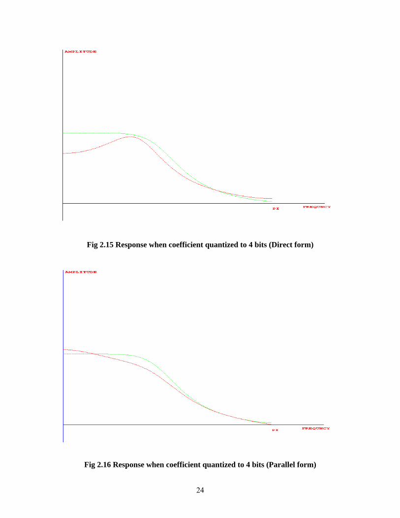
Fig 2.15 Response when coefficient quantized to 4 bits (Direct form)
Fig 2.16 Response when coefficient quantized to 4 bits (Parallel form)
24

2.2 Effects of coefficient quantization in FIR system
For FIR system, we have to concerned with locations of zeros only, since for
causal FIR system all poles are at z = 0. Although we have just seen that direct form
structure should be avoided for high order IIR system, it turns out that direct form
structure is commonly used for FIR systems. To understand why this is so, we express
the system function for a direct form FIR system in the form
∑=
−=M
n
nznhzH0
][)(
Now suppose that the coefficients h[n] are quantized, resulting in a new set of
coefficients ĥ[n] = h[n] + ∆h[n]. The system function for quantized system is then
)()(][)(ˆ0
zHzHznhzHM
n
n ∆+== ∑=
−
Where
nM
nznhzH −
=∑∆=∆
0][)(
Thus, system function of the quantized system is linearly related to the quantization
errors in the impulse response coefficients.
If the zeros of H (z) are tightly clustered, then their locations will be highly
sensitive to quantization errors in the impulse response coefficients. The reason that
direct form FIR system is widely used is that for most linear phase FIR filters, the zeros
are more or less uniformly spread in the z-plane.
Designing of FIR low pass filter using Parks-McClellan design technique
Pass band ripple: 0.99
Stop band ripple: 0.001
Pass band frequency: 1.2566
Stop band frequency: 1.885
25

Fig 2.17 FIR quantization example (a) Log magnitude for unquantized case;
Approximation error for (b) unquantized case (c) 16 bit quantization [1]
Fig 2.17 (continued) Approximation error for (d) 14 bit quantization (e) 13 bit
quantization (f) 8 bit quantization [1]
26
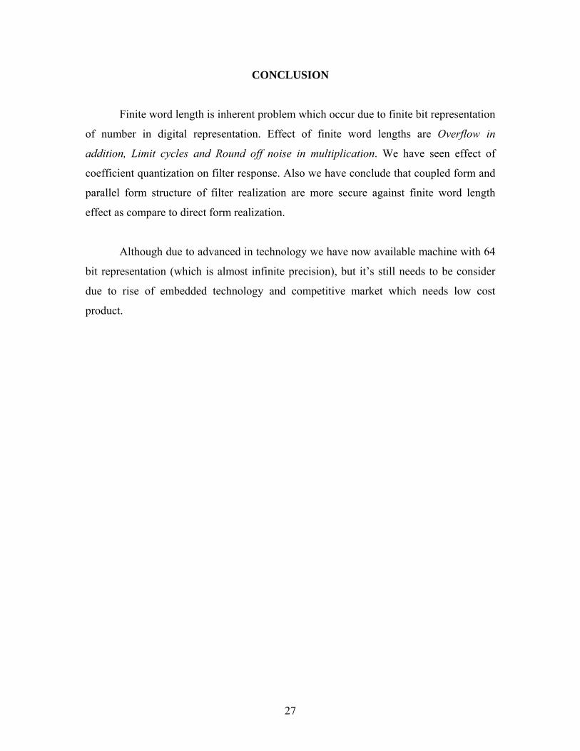
CONCLUSION
Finite word length is inherent problem which occur due to finite bit representation
of number in digital representation. Effect of finite word lengths are Overflow in
addition, Limit cycles and Round off noise in multiplication. We have seen effect of
coefficient quantization on filter response. Also we have conclude that coupled form and
parallel form structure of filter realization are more secure against finite word length
effect as compare to direct form realization.
Although due to advanced in technology we have now available machine with 64
bit representation (which is almost infinite precision), but it’s still needs to be consider
due to rise of embedded technology and competitive market which needs low cost
product.
27

REFERENCES
• Discrete Time Signal Processing, Oppenheim A. V and Schafer R. W., Prentice-Hall.
• Digital Signal Processing, John G. Proakis and Dimitris G. Manolakis, Prentice-Hall.
• Numerical Recipes in C, The Art of Scientific Computing William H. Press, Saul A.
Teukolsky, William T. Vetterling, P. Flannery, Second Edition, Cambridge University
Press..
• Digital Signal Processing, A Computer-Based Approach, Sanjit K. Mitra, McGraw
Hill, Second Edition.
• http://cnx.rice.edu/content/coll10259/latest/
• http://embedded.com/97/feat9707.html
• http://spectrumdi.com/ch4.pdf
28