Embed Size (px)
Citation preview
FINNISH METEOROLOGICAL INSTITUTE
CONTRIBUTIONS
No. 42
GEOMAGNETIC INDUCTION DURING HIGHLY DISTURBED
SPACE WEATHER CONDITIONS: STUDIES OF GROUND
EFFECTS
Antti Pulkkinen
Department of Physical Sciences
Faculty of Science
University of Helsinki
Helsinki, Finland
ACADEMIC DISSERTATION in physics
To be presented, with the permission of the Faculty of Science of the University ofHelsinki, for public critisism in Small Auditorium E204 at Physicum in Kumpula Cam-pus on August 30th, 2003, at 10 a.m.
Finnish Meteorological InstituteHelsinki, 2003

ISBN 951-697-579-8 (paperback)ISBN 952-10-1253-6 (pdf)
ISSN 0782-6117
YliopistopainoHelsinki, 2003

Series title, number and report code of publication Published by Finnish Meteorological Institute Contributions 42, FMI-CONT-42 P.O. Box 503
FIN-00101 Helsinki, Finland Date June 2003 Authors Name of project Antti Pulkkinen
Commissioned by Title Geomagnetic induction during highly disturbed space weather conditions: Studies of ground effects Abstract The thesis work tackles the end of the space weather chain. By means of both theoretical and data-based investi-gations the thesis provides new tools and physical understanding of the processes related to geomagnetic induc-tion and its effects on technological systems on the ground during highly disturbed geomagnetic conditions. In other words, the thesis focuses on geomagnetically induced currents (GIC). Noteworthy is also that GIC research is a practical interface between the solid Earth and space physics domains. It is shown that GIC can be modeled accurately with rather simple mathematical tools requiring that the topology and the electrical parameters of the conductor system, the ground conductivity structure and either the ionospheric source current or the ground magnetic field variations are known. Data-based investigations revealed that from the geophysical viewpoint, the character of GIC events is twofold. On one hand, large GIC can be observed at the same time instant throughout the entire auroral region. On the other hand, spatial and temporal scales related to these events are rather small making the detailed behavior of individual GIC events relatively local. It was ob-served that although substorms are statistically the most important drivers of large GIC in the auroral region, there are a number of different magnetospheric mechanisms capable to such dynamic changes that produce large GIC. Publishing unit Geophysical Research Classification (UDC) Keywords 52-85, 550.38 Geomagnetically induced currents, geomagnetic
disturbances, space weather ISSN and series title 0782-6117 Finnish Meteorological Institute Contributions ISBN Language 951-697-579-8(paperback), 952-10-1253-6(pdf) English Sold by Pages 164 Price
Finnish Meteorological Institute / Library P.O.Box 503, FIN-00101 Helsinki Note Finland

Julkaisun sarja, numero ja raporttikoodi Contributions 42, FMI-CONT-42 Julkaisija Ilmatieteen laitos
PL 503, 00101 Helsinki Julkaisuaika Kesäkuu 2003 Tekijä(t) Projektin nimi Antti Pulkkinen
Toimeksiantaja Nimeke Voimakkaiden avaruussäämyrskyjen vaikutukset maanpinnan teknologisiin johdinjärjestelmiin Tiivistelmä Väitöstyö käsittelee avaruussääketjun loppupäätä, geomagneettisten häiriöiden vaikutuksia maanpinnan teknologisiin johdinjärjestelmiin. Toisin sanoen työssä tarkastellaan geomagneettisesti indusoituneita virtoja (GIC). Työ tuo teoreettisten ja havaintoihin perustuvien tarkastelujen avulla sekä uusia työkaluja että uutta fysikaalista ymmmärrystä avaruusään maanpintavaikutuksiin. Työ osoittaa konkreettisesti kuinka GIC-tutkimus on rajapinta avaruusfysiikan ja maaperän tutkimuksen väillä. Väitöstyö osoittaa, että GIC:tä voidaan mallintaa tarkasti varsin yksinkertaisten matemaattisten menetelmien avulla. Mallinnus edellyttää, että johdinjärjestelmän topologia ja sähköiset ominaisuudet, maan johtavuusrakenne ja ionosfäärin virtojen tai maanpinnan magneettikentän käyttäytyminen tunnetaan. Havaintoihin perustuvat tarkastelut paljastivat, että GIC-ilmiö on geofysikaalisilta ominaisuuksiltaan kaksijakoinen. Toisaalta suuria induktiovirtoja voidaan havaita samaan aikaan kaikkialla revontulialueella. Toisaalta taas ilmiöön liittyvät aika- ja paikkaskaalat ovat verrattain pieniä, joten GIC:n yksityiskohtainen käyttäytyminen on hyvin paikallista. Havaittiin, että vaikkakin geomagneettiset alimyrskyt ovat tilastollisesti kaikkein merkittävin suurien GIC:den aiheuttaja, myös lukuisat muut magnetosfäärin dynaamiset muutokset voivat aiheuttaa merkittäviä vaikutuksia maanpinnan teknologisissa johdinjärjestelmissä. Julkaisijayksikkö Geofysiikka Luokitus (UDK) Asiasanat 52.85, 550.38 Geomagneettisesti indusoituneet virrat, geomagneettiset häiriöt, avaruussää ISSN ja avainnimike 0782-6117 Finnish Meteorological Institute Contributions ISBN Kieli 951-697-579-8(paperback), 952-10-1253-6(pdf) englanti Myynti Sivumäärä 164 Hinta Ilmatieteen laitos / Kirjasto PL 503, 00101 Helsinki Lisätietoja

Preface
In the wake of the emerging science of space weather, the effects of our nearspace environment on technological systems both on the ground and in spacehave received growing attention through the late 1990’s and beginning of thenew millennium. Because of the apparent attractiveness of the subject, largenumber of recent scientific work has fallen, or been dropped, under the realmof space weather and even commercial companies have been established toserve the interests of the industry. However, despite the existing commercialactivities, the size of the market for such a service is not yet well knownand is under a constant debate. In addition, there is still no definite pictureabout the true nature of the risk that space weather related phenomena poseon different systems. The presently ongoing Space Weather Pilot Projectsfunded by the European Space Agency, will hopefully enlighten the sizeof the space weather market and give some quantitative measures for theimpact of space weather on technological systems in the near future.
Regardless of the economical importance, space weather can be thoughtof as an ultimate test of our scientific understanding about our near spaceand its coupling to the Earth surface environment, and is by far the mostimportant motivation for the thesis at hand. In order to be able to model,and eventually, forecast, the Earth surface effects due to some specific eventon the Sun, we have to be able to describe in quite good detail the physi-cal behavior of the entire Sun - solar wind - magnetosphere - ionosphere -ground chain. The chain is governed by processes which require a numberof different physical approaches, and it is clear that convergence of multi-disciplinary science is needed before a consistent picture of the phenomenacan emerge. Space weather is an umbrella unifying different branches ofscience for establishing a collective picture of our constantly broadening en-vironment.
The thesis presented addresses the end link of the space weather chain.By means of both theoretical and data-based investigations the thesis at-tempts to provide new tools and physical understanding of the processes
i

ii PREFACE
related to geomagnetic induction and its effects on technological systemson the ground during highly disturbed geomagnetic conditions. In otherwords, the thesis focuses on geomagnetically induced currents (GIC), to usethe general term given for the phenomena.
The work done in the thesis is presented in five papers published in in-ternational journals. The papers are the following:
I) Pulkkinen, A., R. Pirjola, D. Boteler, A. Viljanen, and I. Yegorov, Mod-elling of space weather effects on pipelines, Journal of Applied Geophysics,48, 233, 2001a.
II) Pulkkinen, A., A. Viljanen, K. Pajunpaa, and R. Pirjola, Recordingsand occurrence of geomagnetically induced currents in the Finnish naturalgas pipeline network, Journal of Applied Geophysics, 48, 219, 2001b.
III) Pulkkinen, A., O. Amm, A. Viljanen, and BEAR Working Group,Ionospheric equivalent current distributions determined with the method ofspherical elementary current systems, Journal of Geophysical Research, 108,doi: 10.1029/2001JA005085, 2003a.
IV) Pulkkinen, A., A. Thomson, E. Clarke, and A. McKay, April 2000geomagnetic storm: ionospheric drivers of large geomagnetically inducedcurrents, Annales Geophysicae, 21, 709, 2003b.
V) Pulkkinen, A., O. Amm, A. Viljanen, and BEAR Working Group, Sep-aration of the geomagnetic variation field on the ground into external andinternal parts using the spherical elementary current system method, Earth,Planets and Space, 55, 117, 2003c.
Summarizing, the work made in these papers is:
I) An extension of the distributed source transmission line (DSTL) theory(Boteler and Cookson, 1986) was introduced to the computation of the in-duced currents and pipe-to-soil voltages in complex pipeline networks. Themethod was tested by three-dimensional simulations and by comparing mea-sured and modeled GIC.
II) The method developed in Paper I was applied to the Finnish natu-ral gas pipeline. Using measurements of GIC in the pipeline, carried outby the Finnish Meteorological Institute, and recordings of the geomagnetic
iii
field at the Nurmijarvi Geophysical Observatory, statistical occurrence forGIC and pipe-to-soil voltages at different parts of the Finnish pipeline werederived.
III) A novel Spherical Elementary Currents System (SECS) method devel-oped by Amm (1997) and Amm and Viljanen (1999) for the determinationof ionospheric equivalent currents was rigorously tested for applications withdata from the BEAR and IMAGE magnetometer arrays. A combined ap-plication of the SECS and complex image method (CIM) for geomagneticinduction studies was introduced. The June 26, 1998 event was investigated.
IV) GIC and magnetic data from northern Europe with ionospheric equiv-alent currents derived applying the SECS method were used to investigateionospheric drivers of GIC during the April 6-7, 2000 geomagnetic storm. Asolid component of the work was the investigation by Huttunen et al. (2002)where the entire Sun - solar wind - magnetosphere - ionosphere chain wasstudied for this storm. Additional conclusions were drawn using statisticsderived from the GIC measurements in the Finnish pipeline.
V) The SECS method was applied to the magnetic field separation problem.Using synthetic ionospheric current models and image currents mimickingthe Earth response, the new method was tested for applications with BEARand IMAGE magnetometer arrays. Data from the BEAR period were usedto separate the field for real events and the results were discussed.
The core of the thesis is composed of the attached five papers. Thepurpose of the introductory part of the thesis is to give the basic back-ground relevant for understanding the topics discussed in the papers andto relate the work made in them to a ”bigger” context of solid Earth andsolar-terrestrial physics. Repeating text from the attached papers is avoidedwhenever reasonable, and the reader is preferably referred to an appropriatepaper for more detailed discussions.
In Chapter 1, general phenomena of space weather and its role for ourenvironment are briefly outlined and some of the non-ground effect aspectsare discussed. However, the emphasis of the chapter is mainly on a relativelylow-level introduction to the ground induction effects of space weather. Lightis shed on the basic physics behind the effects and on how different tech-nological systems are affected. In Chapter 2, the general theoretical basisand the modeling artillery used in quantitative GIC investigations are pre-
iv PREFACE
sented. The aim of the chapter is to furnish a rather complete treatmentof the physics relevant for GIC. This means, that if the basic relation rel-evant to our discussion is not derived in one of the attached publications,the derivation is given here starting from first principles. In the last sec-tion of the chapter, a unification of the mathematical methods applicablefor GIC investigations is introduced. In Chapter 3 the characteristics of theGIC phenomena are discussed in the context of the work done in the thesis.Though the two sections of the chapter, one on geoelectric fields and anotheron ionospheric currents, are rather closely related, a separate treatment ispursued for clarity. Finally, in Chapter 4 the theses of the work are givenand the challenges for future GIC investigations are briefly discussed.
This thesis work was carried out at the Geophysical Research Division(GEO) of the Finnish Meteorological Institute (FMI). A number of peopledeserve my sincere gratitude. First I would like to thank Professors RistoPellinen and Tuija Pulkkinen, the former and the acting Director of GEO,respectively, as well as Prof. Erkki Jatila and Dr. Petteri Taalas, the for-mer and the present Director General of FMI, respectively, for providingexcellent working conditions. The successful completion of the work wouldnot have been possible without the talented and effective supervisor Dr.Ari Viljanen, whose MatLab programs did great deal of the work presentedin this thesis. The unofficial supervisors Drs Olaf Amm and Risto Pirjolahave put lot of work (along with A. Viljanen) into discussing numerous the-oretical and other issues related to the thesis and in correcting the worsterrors in my grammar. R. Pirjola is acknowledged also for being a flexibleand encouraging head of the Space Physics Research Group and for saying:”next is the last” - after the ”last” one in numerous places for sufficientnumber of times. Besides the colleagues in Finland and elsewhere that Ihave had the chance to work with, I would like to acknowledge Gasum Oyand Fingrid Oyj, the owners of the Finnish natural gas pipeline and thehigh-voltage transmission system, respectively, for their continuous supportfor the Finnish GIC research. The reviewers of the thesis, Prof. WolfgangBaumjohann and Dr. Jurgen Watermann are gratefully acknowledged. Thework was financially supported by the Academy of Finland.
There is also life beyond work, though the boundary between the workand ”other things” can sometimes be rather fuzzy. My lovely partner, Katja”Muori” Mikkonen knows only too well what this means. She is the one whobore evenings in the sound of typing and angry curses. Muori, I cannot thankyou enough for your patience and support. The greatest rock’n’roll band inthe history of space science, Geodynamo, is acknowledged for giving tinnitusand unforgettable moments on the stage. I am also indebted to Mega Duty
v
weightlifting sessions with Ari-Matti Harri that were the extra piece of funthat kept me going both mentally and physically. Finally, I would like tothank my family and friends who along with Muori form the strongest andthe most important building block of my life.
A. PulkkinenHelsinki, Finland
June, 2003

vi PREFACE

Notations
Below are listed the symbols and acronyms used in the work. Vector quan-tities are denoted by bold letters. SI units are used throughout the work.
E electric field in the spatial domaine electric field in the spectral domainB magnetic field in the spatial domain.b magnetic field in the spectral domain.j electric current densityJ electric sheet current densityJcf curl-free sheet currentsJdf divergence-free sheet currentsJeq equivalent sheet currentsI set of scaling factors of the spherical elementary systemst timeσ electrical conductivityµ0 permeability of the free spaceε0 permittivity of the free spaceRe radius of the EarthZ spectral impedanceZint
ij internal impedance of a transmission lineRij = Re(Zint
ij )Zp impedance per unit length of a pipelineYp admittance per unit length of a pipelineInij current along a transmission line
Iei earthing current
p complex skin depth
BEAR Baltic Electromagnetic Array ResearchCIM complex image methodDSTL distributed source transmission line
vii
viii NOTATIONS
GIC geomagnetically induced currentIMAGE International Monitor for Auroral Geomagnetic EffectsP/S pipe-to-soilSECS spherical elementary current systemSVD singular value decomposition
Contents
Preface i
Notations vii
1 Introduction 31.1 The role of space weather for our environment . . . . . . . . . 31.2 Ground induction effects of space weather . . . . . . . . . . . 6
1.2.1 Physical basis . . . . . . . . . . . . . . . . . . . . . . . 61.2.2 Technological impacts . . . . . . . . . . . . . . . . . . 10
2 Theoretical framework 152.1 Derivation of ionospheric equivalent currents . . . . . . . . . 16
2.1.1 Separation of the ground disturbance magnetic fieldinto external and internal parts . . . . . . . . . . . . . 24
2.2 Computation of the ground geoelectric field . . . . . . . . . . 262.2.1 Computation via surface magnetic field . . . . . . . . 282.2.2 Computation using a known ionospheric current system 35
2.3 Computation of geomagnetically induced currents . . . . . . . 392.3.1 Discretely grounded systems . . . . . . . . . . . . . . 392.3.2 Continuously grounded systems . . . . . . . . . . . . . 45
2.4 Unification of the methods for practical applications . . . . . 46
3 Characteristics of intense GIC events 493.1 Properties of intense meso-scale geoelectric
fields . . . . . . . . . . . . . . . . . . . . . . . . . . . . . . . . 493.2 Properties of ionospheric currents causing intense geoelectric
fields and the linkage to large-scale magnetospheric phenomena 54
4 Discussion 614.1 Theses of the work . . . . . . . . . . . . . . . . . . . . . . . . 61
1

2 CONTENTS
4.2 New challenges . . . . . . . . . . . . . . . . . . . . . . . . . . 62

Chapter 1
Introduction
1.1 The role of space weather for our environment
There is weather also in space. Although there are on average only few par-ticles per cubic centimeter in the solar wind driving the weather in space,the vast size of the system and the complex coupling mechanisms make thisnearly vacuum environment very dynamic and capable to affect our every-day life. Physical processes driving space weather are linked by the chain ofcausal connections starting from processes on the Sun. Quoting James A.Van Allen, after whom the two radiation belts surrounding the Earth arenamed, from the foreword of Carlowicz and Lopez (2002): ”Space weatheris attributable to highly variable outward flow of hot ionized gas (a weaklyionized ”plasma” at a temperature of about 100.000 degrees Kelvin, calledthe solar wind) from the Sun’s upper atmosphere and to nonthermal, spo-radic solar emissions of high-energy electrons and ions and electromagneticwaves in the X-ray and radio portions of the spectrum”. The coupling of theflow of solar wind and nonthermal emissions to the Earth’s magnetosphere,coupled itself to the ionosphere, is obtained via several different physical pro-cesses. The processes relevant in the context of this thesis will be reviewedand discussed below.
The most famous definition for space weather was formulated in 1994during the birth of the US National Space Weather Program (Robinson andBehnke, 2001). It reads as follows:
Space weather refers to conditions on the Sun and in the solar wind, magne-tosphere, ionosphere, and thermosphere that can influence the performanceand reliability of space-borne and ground-based technological systems and can
3

4 CHAPTER 1. INTRODUCTION
endanger human health. Adverse conditions in the space environment cancause disruption of satellite operations, communications, navigation, andelectric power distribution grids, leading to a variety of sosioeconomic losses.
When extended through the notification that mankind can also benefit from(instead of solely suffer from it) good space weather, i.e. with beautifulsights of auroras, the definition is quite comprehensive and describes wellthe basic meaning of space weather. The important point to realize is thatspace weather is a concept that rather than just being another term forsolar-terrestrial physics (STP), combines both technological and scientificaspects of our near space environment.
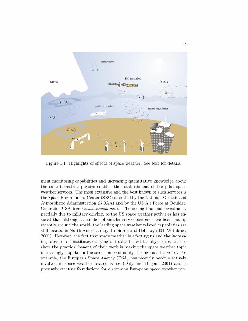
Highlights of some of the adverse effects that space weather has on sys-tems and the mechanisms behind the effects are presented in Fig. 1.1.These include single-event upsets in the spacecraft electronics caused by highenergy protons, electron induced spacecraft surface and internal chargingleading to discharge currents, solar panel degradation due to particle bom-bardment, tissue damages due to particle radiation, increased atmosphericdrag experienced by low orbit spacecraft, disturbances in HF communica-tion and navigation systems caused by the irregularities in the ionosphere,cosmic ray induced neutron radiation at airline hights, geomagnetically in-duced currents (GIC) in long conductor systems on the ground caused byrapidly varying ionospheric currents and lastly one of the hottest topics ingeophysics, the possible modulation of the neutral atmospheric weather byspace weather. For more complete listings see e.g. Lanzerotti at al. (1999);Feynman (2000); Koskinen et al. (2001); Lanzerotti (2001).
The discovery of the telegraph system in the 19th century, was the turn-ing point after which the near space phenomena begun to have direct adverseeffects on man’s daily life. Positive aspects of the phenomena date fartherback in time. The first records of auroras originate from ancient times(fairly continuous from 560 AD onward) from Eastern Asia and Europe(Pang and Yau, 2002). It is obvious, although not unambiguously recorded,that auroras were observed also before. The number of potentially vulner-able systems increased rapidly in the beginning of the 20th century: Wire-less communication applying long wavelength radio transmissions, complexhigh-voltage power transmission networks and long trans-Atlantic telecom-munication cables, and eventually orbiting spacecraft were all found to beaffected by space weather. Thus there appeared growing need for deeperunderstanding of the phenomena and even for the establishment of servicesproviding space weather related information to the operators of the affectedtechnological systems. In the 1990’s, the enhancement of near space environ-
5
B(r,t)
)j (r,tn (r,t)
E(r,t)
air dragS/C anomalies
signal degradation
cosmic rays
GIC
particle radiation
auroras
Figure 1.1: Highlights of effects of space weather. See text for details.
ment monitoring capabilities and increasing quantitative knowledge aboutthe solar-terrestrial physics enabled the establishment of the pilot spaceweather services. The most extensive and the best known of such services isthe Space Environment Center (SEC) operated by the National Oceanic andAtmospheric Administration (NOAA) and by the US Air Force at Boulder,Colorado, USA (see www.sec.noaa.gov). The strong financial investment,partially due to military driving, to the US space weather activities has en-sured that although a number of smaller service centers have been put uprecently around the world, the leading space weather related capabilities arestill located in North America (e.g., Robinson and Behnke, 2001; Withbroe,2001). However, the fact that space weather is affecting us and the increas-ing pressure on institutes carrying out solar-terrestrial physics research toshow the practical benefit of their work is making the space weather topicincreasingly popular in the scientific community throughout the world. Forexample, the European Space Agency (ESA) has recently become activelyinvolved in space weather related issues (Daly and Hilgers, 2001) and ispresently creating foundations for a common European space weather pro-

6 CHAPTER 1. INTRODUCTION
gram via targeted pilot services. Space weather related research efforts havealso started within the European Union. Consequently, the US lead in spaceweather related research and services is likely to narrow in the future, andmore importantly, the present international efforts guarantee that the recenttrend of growing popularity of space weather will remain.
1.2 Ground induction effects of space weather
1.2.1 Physical basis
After installation of the first telegraph systems in the 1830’s and 1840’s, itwas noticed that from time to time there were electric disturbances driv-ing such large ”anomalous” currents in the system that the transmissionsof the messages was extremely difficult while at other times no battery wasneeded for the operation (e.g., Barlow, 1849; Prescott, 1866). For exam-ple, the famous September 1859 geomagnetic storm (term introduced byAlexander von Humboldt in the 1830’s) produced widespread disturbancesin the telegraph systems in North America and Europe. The disturbancescoincided with the solar flare observations of Carrington and auroral ob-servations all over the world (Loomis, 1859; Carrington, 1860) and led tospeculations about the possible connection between these phenomena. How-ever, the physical explanation remained unclear for the next half century.Eventually, in the late 19th century the experimental evidence build up andconfirmed the relation between the solar, auroral and ground magnetic phe-nomena. During the First Polar Year (1882-1883) scientists defined magneticstorms as intense, irregular variations of the geomagnetic field which occuras a consequence of solar disturbances (e.g., Kamide, 2001). The work byBirkeland, Størmer and Chapman, although differing in details, suggestedthat the origin for variations of the ground magnetic field was in the electriccurrents in space and that the currents in turn were created by the interac-tion between the magnetic field of the Earth and particles streaming from theSun. The beginning of the space age in the 1950’s made direct observationsof the space environment possible and since then the important discoveriesand confirmations of earlier theories followed quickly each other: The exis-tence of the radiation belts, field-aligned currents coupling the ionosphere tothe magnetosphere, solar wind, solar sources for geomagnetic disturbances(flares, coronal mass ejections, coronal holes). The new information fromthe space and from the growing network of ground magnetic observatoriesfinally made it possible to understand the basics of the the origins and mech-anisms for ground effects of space weather (for a popular presentation see
7
e.g., Carlowicz and Lopez, 2002).Besides the advances in early space physics, significant progress was also
made in understanding the electromagnetic induction of geomagnetic origin(geomagnetic induction) inside the Earth, the ultimate reason for the exis-tence of the currents in ground conductor systems. The basic foundations foradvanced induction studies were laid by Faraday, who discovered in 1830’sthat time varying magnetic fields create currents in electrically conductingmaterials. The first quantitative measure for geomagnetic induction wasgiven by Schuster (1889), who investigated magnetic field related to diurnalvariations and found that a small portion of the field was of internal origin,i.e. caused by the currents induced within the Earth. Also in the inductionstudies the great advances were made after the turn of the 19th century,the work being focused on dealing with increasingly complicated groundconductivity structures (e.g., Lahiri and Price, 1938). However, besides tosomewhat cumbersome scale analogue models (e.g., Frischknecht, 1988), thework with realistic three-dimensional conductivity structures has not beenpossible prior to the advent of large computational power.
Noteworthy is that the main motivation in the majority of the geomag-netic induction studies has been in deducing the electrical properties of theEarth from the measured magnetic field variations. Though the basic sourcemorphology has been investigated (e.g., Mareschal, 1986), the actual sourceprocesses for these variations has been of relatively little interest. Thus untilthe present days, there has been a substantial gap between the geomagneticinduction and space physics communities regardless the physical connectionbetween the two. Space weather is a link between the disciplines, as can beseen from the work at hand.
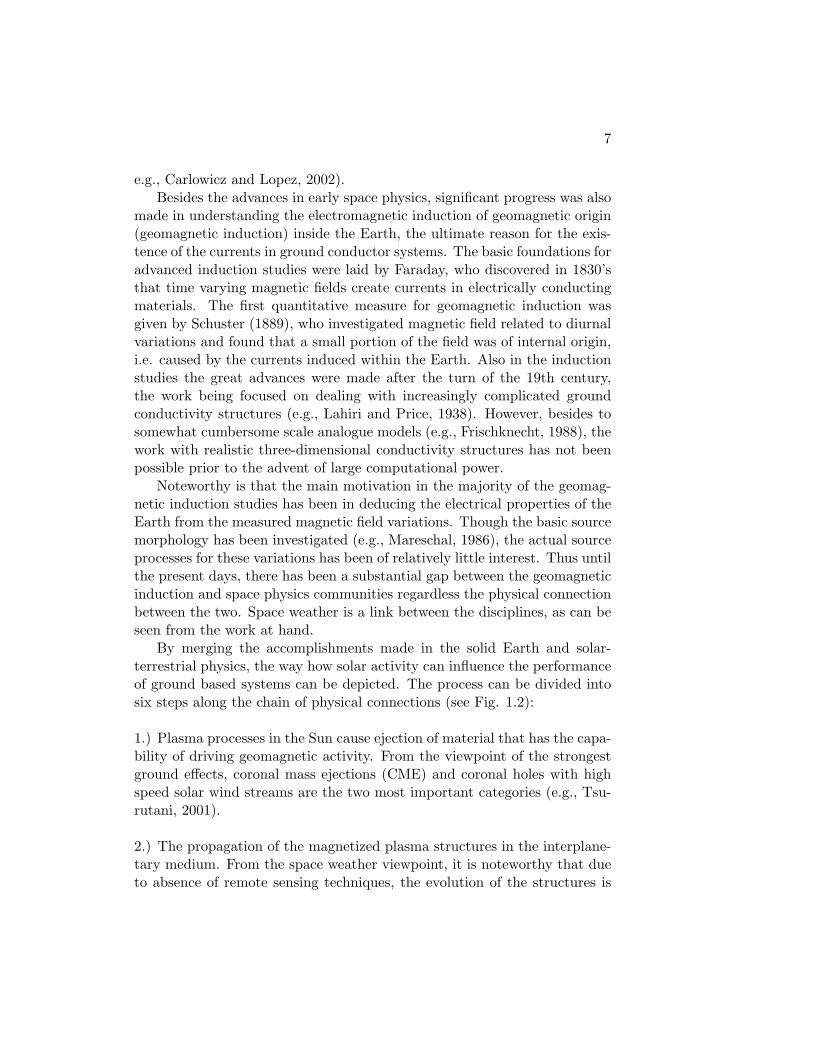
By merging the accomplishments made in the solid Earth and solar-terrestrial physics, the way how solar activity can influence the performanceof ground based systems can be depicted. The process can be divided intosix steps along the chain of physical connections (see Fig. 1.2):
1.) Plasma processes in the Sun cause ejection of material that has the capa-bility of driving geomagnetic activity. From the viewpoint of the strongestground effects, coronal mass ejections (CME) and coronal holes with highspeed solar wind streams are the two most important categories (e.g., Tsu-rutani, 2001).
2.) The propagation of the magnetized plasma structures in the interplane-tary medium. From the space weather viewpoint, it is noteworthy that dueto absence of remote sensing techniques, the evolution of the structures is
8 CHAPTER 1. INTRODUCTION
Solar wind propagation
Solar wind - magnetosphereinteraction
Magnetosphere - ionosphereinteraction
Ionosphere - groundinteraction (induction)
Geoelectric field - GIC
Solar ejections
Solar wind propagation
Solar wind - magnetosphereinteraction
Magnetosphere - ionosphereinteraction
Ionosphere - groundinteraction (induction)
Geoelectric field - GIC
Solar ejections
Figure 1.2: Six steps of space weather chain from the Sun to the ground.
very difficult to estimate.
3.) Interaction between the solar wind (or structures within) and magneto-sphere (Fig. 1.3). Here the dominant factor for determining the geoeffective-ness of the structure is the orientation of the solar wind magnetic field, i.e.how much southward the field is. The energy feed into the magnetosphere ishighest during strong reconnection of the solar wind and the magnetosphericmagnetic fields. Increased energy input to the system sets the conditions fordynamics changes in the magnetospheric electric current systems. One ofsuch dynamic changes are magnetic storms which are characterized by en-hanced convection of the magnetospheric plasma and enhanced ring currentcirculating the Earth (see e.g., Tsurutani and Gonzalez, 1997).
4.) Magnetosphere-ionosphere interaction. The closure of the magneto-spheric currents systems goes via polar regions of the ionosphere. Corre-spondingly, dynamic changes in the magnetospheric current systems coupleto the dynamics of the ionosphere. An important class of dynamic varia-tions are auroral substorms which are related to loading-unloading processesin the tail of the magnetosphere (e.g., Kallio et al., 2000). During auroral

9
BIMF shock
solarwind
magnetopause
t < 0 t = 0 t > 0t < 0 t = 0 t > 0
(a)
(b) (c)
Figure 1.3: (a) Interaction process between the solar wind magnetic fieldBIMF , i.e. interplanetary magnetic field and Earth’s magnetic field. (b) Re-connection between the magnetic field of these two regions changes the fieldtopology and transports energy into the magnetosphere. (c) Another recon-nection site in the night-side magnetosphere separates the interplanetaryand the magnetospheric magnetic fields. Figure adopted from Tanskanen(2002).
substorms particles injected from the tail of the magnetosphere are seen inthe ionosphere in terms of auroras and rapid changes in the auroral currentsystems. Although some of the basic features are understood, the details ofthe storm and substorm processes as well as the storm/substorm relation-ship are one of the most fundamental open questions in the solar-terrestrialphysics (for a review see e.g., Kamide, 2001).
5.) Rapid changes of the ionospheric and magnetospheric electric currentscause variation in the geomagnetic field which according to Faraday’s law ofinduction induce an electric field which drives an electric current in the sub-surface region of the Earth. The nature of this geoelectric field is dependent

10 CHAPTER 1. INTRODUCTION
on the characteristics of the ionospheric-magnetospheric source and on theconductivity structure of the Earth. As a rule of thumb, the magnitude ofthe geoelectric field increases with increasing time derivatives of the groundmagnetic field and with decreasing ground conductivity.
6.) Finally, the geoelectric field drives currents within conductors at andbelow the surface of the Earth. The magnitude and distribution of thecurrents are dependent on the topology and electrical characteristics of thesystem under investigation. The induced currents flowing in technologicalsystems on the ground are called geomagnetically induced currents (GIC).
1.2.2 Technological impacts
The first technological impacts of space weather were seen on telegraphsystems where disturbances in signals and even fires at telegraph stationswere experienced (Harang, 1941). However, in principle all conductors canbe influenced by GIC. Due to the relatively small magnitudes of geoelec-tric fields, with maximum observed values being of the order of 10 V/km(Harang, 1941), only spatially extended systems can be affected.
After the telegraph equipment, the next category of technological con-ductor systems seen to be affected were power transmission systems (thefirst report by Davidson, 1940). Regarding economic impacts, industrialinterests and the number of studies carried out, the effects on power trans-mission systems are, to the present knowledge, the most important categoryof space weather effects on the ground. Solely the impact of the great March1989 storm on power systems in North America was greater than reported inother systems altogether at all times (e.g., Czech et al., 1992; Kappenman,1996). Barnes and Van Dyke (1990) estimated that a blackout in the North-east US for 48 hours would cost as an unserved electricity and replacementsof the damaged equipment from 3 to 6 billion US dollars.
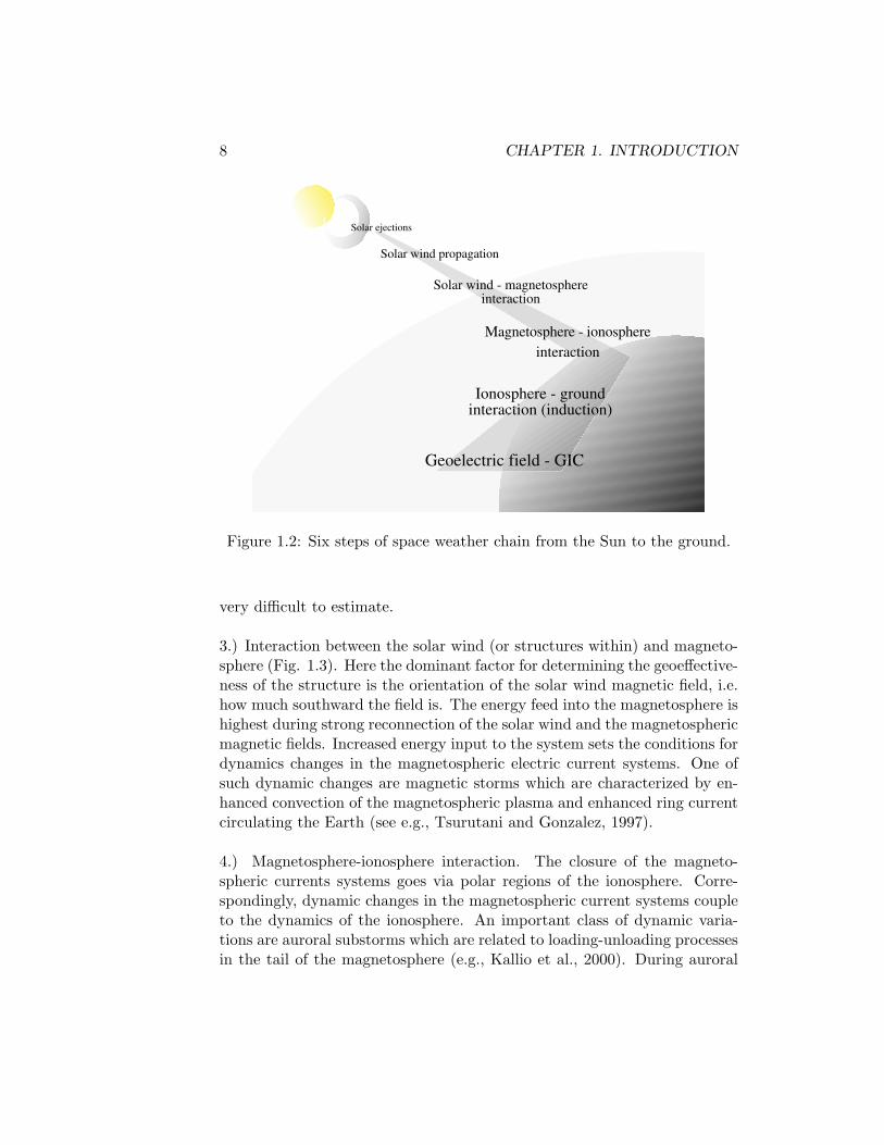
In power transmission systems, the primary effect of GIC is the half-cycle saturation of high-voltage power transformers (e.g. Kappenman andAlbertson, 1990; Molinski, 2002). The typical frequency range of GIC is 1- 0.001 Hz (periods 1 - 1000 s), thus being essentially direct current (dc)for the power transmission systems operating at 60 Hz (North America)and 50 Hz (Europe). (Quasi-)dc GIC causes the normally small excitingcurrent of the transformer to increase even to a couple orders of magnitudehigher values, i.e. the transformer starts to operate well beyond the designlimits (see Fig. 1.4). The saturated transformer causes an increase of thereactive power consumed by the transmission system, ac character of the
11
flux
current{
DC offsetof the flux
{ increase in the amplitude of the exciting current
Figure 1.4: Simplified illustration of the saturation of the transformer. Whenthe magnetic flux inside the transformer is offset by the (quasi-)dc GIC, thetransformer starts to operate in the non-linear portion of the magnetizationcurve, i.e. a small increase in the flux requires a large increase in the excitingcurrent.
power transmission which means that the real power available in the systemis decreasing. Another effect of the saturated transformer is that the 50 or60 Hz waveform is distorted, i.e. the higher harmonic content in the elec-tricity increases. Harmonics introduced to the system decrease the generalquality of the electricity, and may cause false trippings of protective relaysdesigned to switch the equipment off in the case of erratic behavior of thesystem. Trippings of the static VAR compensators (employed to deal withthe changing reactive power consumption) started the avalanche that finallyled to the collapse of the Canadian Hydro-Quebec system on March 13, 1989(e.g., Boteler et al., 1998; Bolduc, 2002).
Also more advanced telecommunication cables than single-wire telegraphsystems have been affected. The principal mode of failure for these systemsare via erroneous action of power apparatus that are used for energizing the
12 CHAPTER 1. INTRODUCTION
repeaters of the cable (Root, 1979). This is why even modern optic fibercables could be affected (Medford et al., 1989). The best known incidentsare the disruption of communications made via TAT-1, the cross-Atlantic(from Newfoundland to Scotland) communication cable in February 1958(Anderson, 1978) and the shutdown of the AT&T L4 cable running in themid-western US in August 1972 (Anderson et al., 1974). In addition tocommunication problems in February 1958, there was a blackout in theToronto area due to a power system failure (Lanzerotti and Gregori, 1986).
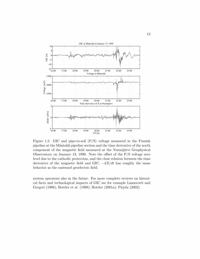
Effects of GIC on pipelines have been of concern since the constructionof the 1280 km long Trans-Alaskan pipeline in the 1970’s (Lanzerotti andGregori, 1986). The flow of GIC along the pipeline is not hazardous but theaccompanying pipe-to-soil (P/S) voltage (see Fig. 1.5) can be a source fortwo different types of adverse effects (e.g., Brasse and Junge, 1984; Boteler,2000; Gummow, 2002). The more harmful effect is related to the currentsdriven by the P/S voltage variations. If the coating, used to insulate thepipeline steel from the soil, has been damaged or the cathodic protection po-tential used to prevent the corrosion current is exceeded by the P/S voltage,the corrosion rate of the pipeline may increase. However, estimates aboutthe time that it takes from the geomagnetic disturbances to seriously dam-age vary quite a lot and no publicly reported failures due to GIC-inducedcorrosion exist (e.g., Campbell, 1978; Henriksen et al., 1978; Martin, 1993).Thus if the pipeline is properly protected against the corrosion, it is likelythat the second and the most important effect of GIC are the problems inmeasuring the cathodic protection parameters and making control surveysduring geomagnetically disturbed conditions.
Although railway systems also have long electrical conductors, it seemsthat malfunctions due to geomagnetic disturbances are very rare. The onlyreported incident is from Sweden, where during a magnetic storm in July1982 traffic lights turned unintendedly red (Wallerius, 1982). Erroneousoperation was explained by the geomagnetically induced voltage that hadannulled the normal voltage, which should only be short-circuited when atrain is approaching leading to a relay tripping. It is, of course, possiblethat some of past ”unknown” railway disturbances have in fact been causedby GIC.
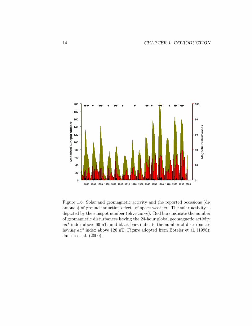
In general, GIC has been a source for problems in technological sys-tems on the ground since the mid 19th century, the number of reports beingroughly a function of the sunspot number and global geomagnetic activity(Fig. 1.6). The number of technological conductor systems is inevitablyincreasing and some of these systems will be built in regions where they canbe affected by GIC. Thus, it is quite obvious that GIC will be of concern for
13
16:00 17:00 18:00 19:00 20:00 21:00 22:00 23:00-15
-10
-5
0
5
10GIC at Mäntsälä in January 13, 1999
GIC
[A]
16:00 17:00 18:00 19:00 20:00 21:00 22:00 23:00
-2500
-2000
-1500Voltage at Mäntsälä
Vol
tage
[m
V]
16:00 17:00 18:00 19:00 20:00 21:00 22:00 23:00-5
0
5Time derivative of X at Nurmijärvi
UT [h]
-dX
/dt
[nT
/s]
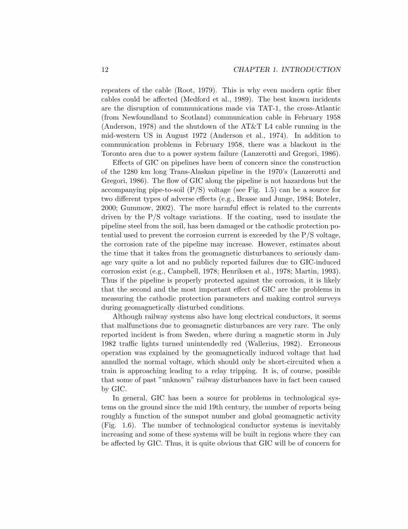
Figure 1.5: GIC and pipe-to-soil (P/S) voltage measured in the Finnishpipeline at the Mantsala pipeline section and the time derivative of the northcomponent of the magnetic field measured at the Nurmijarvi GeophysicalObservatory on January 13, 1999. Note the offset of the P/S voltage zerolevel due to the cathodic protection, and the close relation between the timederivative of the magnetic field and GIC. −dX/dt has roughly the samebehavior as the eastward geoelectric field.
system operators also in the future. For more complete reviews on histori-cal facts and technological impacts of GIC see for example Lanzerotti andGregori (1986); Boteler et al. (1998); Boteler (2001a); Pirjola (2002).
14 CHAPTER 1. INTRODUCTION
1850 1860 1870 1880 1890 1900 1910 1920 1930 1940 1950 1960 1970 1980 1990 2000
Year
0
20
40
60
80
100
120
140
160
180
200
Sm
oo
thed
Su
nsp
ot
Nu
mb
er
0
20
40
60
80
100
Mag
net
ic D
istu
rban
ces
Figure 1.6: Solar and geomagnetic activity and the reported occasions (di-amonds) of ground induction effects of space weather. The solar activity isdepicted by the sunspot number (olive curve). Red bars indicate the numberof geomagnetic disturbances having the 24-hour global geomagnetic activityaa* index above 60 nT, and black bars indicate the number of disturbanceshaving aa* index above 120 nT. Figure adopted from Boteler et al. (1998);Jansen et al. (2000).
Chapter 2
Theoretical framework
The modeling of GIC in specific technological systems is usually divided intotwo independent steps:
1.) Calculation of the surface horizontal geoelectric field based on the know-ledge of the ionospheric source currents and of the ground conductivity struc-ture. As a sub-step, we may need to derive the ionospheric source currentfirst.
2.) Calculation of GIC based on the knowledge of the surface geoelectricfield and of the topology and electrical parameters of the technological con-ductor system under investigation.
The independence of these two steps is based on the assumption that theinductive coupling between the Earth and the technological conductor sys-tem can be neglected. This may seem to be quite a severe assumption atfirst glance but as will be seen below, the coupling is not very strong at thefrequencies of our interest (< 1 Hz) and is thus a second order effect from theGIC modeling point of view. If the coupling is not neglected, the treatmentbecomes complex and very restricting assumptions, like an infinite lengthof the conductor, are needed to keep the problem mathematically tractable.This is the basic problem of GIC modeling, and perhaps more generally inall geophysical modeling: One is forced to search for pragmatic approacheswhere a variety of quite substantial approximations are made. However, inthe GIC modeling the needed approximations are relatively feasible. Forexample, the locality of the studies justifies the flat-Earth assumption, andintegration of the surface electric field made in computing GIC results in
15

16 CHAPTER 2. THEORETICAL FRAMEWORK
that only meso-scale (∼ 100 km) fields and ground conductivity structuresare of interest to us. Furthermore, any higher accuracy than one amperefor the GIC amplitude is not needed. Getting the overall picture is farmore important. This is explained in greater detail in Chapter 3 where thecharacteristics of intense GIC events are discussed.
Assuming that the decomposition of the GIC modeling problem can bemade as stated above, we approach the two steps as separate problems. InSections 2.1 and 2.2 we consider the geophysical step, i.e. determination ofthe ionospheric source currents and the calculation of the surface geoelectricfield, respectively. In Section 2.3 we treat the engineering step, i.e. thecalculation GIC in different technological systems.
2.1 Derivation of ionospheric equivalent currents
Ionospheric equivalent currents are a convenient way to model the iono-spheric source from the geomagnetic induction viewpoint. Although theyare not identical to the true three-dimensional ionospheric current system,they produce the same magnetic effect at the surface of the Earth as the truesystem. Examples of the usage of equivalent currents in induction studieswill be seen later on in Chapter 3. First, however, we see how ionosphericequivalent currents are determined using ground magnetic data.
If the ionosphere were immediately above the surface of the Earth andthe geometry were Cartesian, the equivalent currents Jeq (A/m) situatedon a infinitely thin sheet, could be obtained just by rotating the groundhorizontal magnetic field vector 90 degrees clockwise and by multiplying with2/µ0 where µ0 is the permeability of the free space. However, if the standardapproximation, regarding the ionosphere as a two-dimensional spherical shellat the 110 km height, is used, the situation is more complex and moresophisticated methods are required.
A number of methods, like spherical harmonic (Chapman and Bartels,1940), spherical cap harmonic (Haines, 1985) and Fourier (Mersmann et al.,1979) methods, have been applied to the determination of the ionosphericequivalent currents. However, all of them suffer from drawbacks that canbe avoided by applying the spherical elementary current system (SECS)method. Furthermore, as will be seen in Section 2.2.2, the SECS methodcan be combined with the complex image method used for the quick de-termination of the electromagnetic field at the surface of the Earth. Thisfeature is of significant importance for GIC-related induction studies since itpermits the utilization of realistic ionospheric sources. For a more detailed
17
discussion on advantages of the SECS method compared to the traditionalmethods, see the introduction of Paper III. The mathematical foundationsof the SECS method were established by Amm (1997); Amm and Vilja-nen (1999). Below we briefly outline the method and its usage with thegeomagnetic data.
In the SECS method, we compose ionospheric sheet currents from thedivergence-free and curl-free parts of the vector field. This is similar torepresenting the current by other elementary systems like magnetic dipoles(e.g., Weaver, 1994, p. 12-15), or by current loops having an east-west andnorth-south directed ionospheric part and closing in the magnetosphere asin Kisabeth and Rostoker (1977). However, elementary systems used hereare more fundamental in that they by their basic structure represent thedivergence and the curl of the horizontal current system. Furthermore, aswill be seen below, only the divergence-free part of the currents is neededto represent equivalent currents, thus reducing the number of degrees offreedom by a factor of two.
According to the Helmholtz theorem, any vector field can be decomposedinto divergence-free (df) and curl-free (cf) parts (see e.g. Arfken and Weber,1995, p. 92-97). Or vice versa, if we know the divergence and the curl of avector field and its normal component over the boundary, the field itself isuniquely determined. This allows us to represent the ionospheric currents,assumed to flow in an infinitely thin spherical shell of radius RI (measuredfrom the Earth’s centre), as
J(s) = Jdf (s) + Jcf (s) (2.1)
where
∇h · Jdf (s) = 0 (2.2)[∇× Jcf (s)]r = 0 (2.3)
and
[∇× Jdf (s)]r = u(s) (2.4)∇h · Jcf (s) = v(s) (2.5)
where s is the vector giving coordinates on the shell (see Fig. 2.1) and u andv are the source terms. Note that in Eqs. (2.2)-(2.5) the radial derivative ofthe sheet current is not well defined and thus the divergence is taken onlyfor the horizontal components (∇h) and only the radial component of the

18 CHAPTER 2. THEORETICAL FRAMEWORK
curl is taken into account. Physically, v in Eq. (2.5) can be interpreted as afield-aligned current density (A/m2).
Now let us seek solutions for Jdf and Jcf in Eq. (2.1) using conditions(2.2)-(2.5). The problem can be treated in separate parts; we first deal withJcf . Generally, using Green’s functions we may write
Jcf (s) =∫
SGcf (s, s0)v(s0)ds0 (2.6)
where∇h ·Gcf (s, s0) = δ(s− s0)−
14πR2
I
(2.7)
and δ is a standard Dirac delta function. By taking the divergence of (2.6)and substituting Eq. (2.7) we may verify that the condition (2.5) is fulfilled ifwe require that the total three-dimensional current system is divergence-free(what comes in, must go out), i.e.∫
Sv(s0)ds0 = 0 (2.8)
Relation (2.7) describes the elementary source for the curl-free part of thevector field in (2.1). Apart from the traditional point source seen for examplein the treatment of the electrostatic problem (see e.g., Arfken and Weber,1995, p. 510-512), we have an elementary source composed of both a pointsource at s and a uniform outflow distributed over the surface S (See Fig.2.2). The uniform outflow results in locality of the elementary source andis needed in spherical geometry to fullfill the divergence-free condition ofa single source. Another choice for the elementary source could have beensuch that the inward and outward flows are at the antipoloidal points onthe spherical ionosphere (Fukushima, 1976). However, this type of currentsystem couples the opposite sides of the ionosphere and is not as general asthe choice made here.
If we can solve Gcf defined by (2.7) then we are able to compute Jcf viaRelation (2.6). The problem can be simplified by defining
Gcf (s, s0) = Q−1(s, s0)Gelcf (Q(s, s0)s) (2.9)
where Q is an operator carrying out the changes between a common coor-dinate system having a pole at N (see Fig. 2.1) and a coordinate systemhaving pole at s0. We denote the vector in the coordinate system havingpole at s0 by s′ = Q(s, s0)s. The explicit form of the operator Q will begiven below. The basic idea in Eq. (2.9) is that by the rotation of the

19
N
S
er
eυ
eϕ
υ´
υ
( , )υ ϕs =0 0
( , )υ ϕs =0
Figure 2.1: Coordinate system used in deriving spherical elementary currentsystem method.
coordinate system we are able to reduce the determination of Gcf to thedetermination of function of one variable, i.e. to determination of Gel
cf (ϑ′).We define s = (ϑ, ϕ) where ϑ and ϕ are the polar and azimuth angles, re-spectively. Now in the coordinate system having pole at s0 = (ϑ0, ϕ0) it issimple to show that Eq. (2.7) with the boundary condition Gel
cf (ϑ′ = π) = 0is fulfilled by the function
Gelcf (ϑ′) =
14πRI
cot(ϑ′/2)eϑ′ (2.10)
where ϑ′ is the angle between s = (ϑ, ϕ) and s0 = (ϑ0, ϕ0) (see Fig. 2.1) andeϑ′ is the unit vector in the coordinate system having pole at s0 = (ϑ0, ϕ0).Eq. (2.10) for Gel
cf with the operator Q enables the computation of thegeneral Gcf in Eq. (2.9) and thus the evaluation of Eq. (2.6). The problemfor the curl-free part is solved.
The divergence-free part Jdf is handled completely analogously to thecurl-free case. We obtain
Geldf (ϑ′) =
14πRI
cot(ϑ′/2)eϕ′ (2.11)
20 CHAPTER 2. THEORETICAL FRAMEWORK
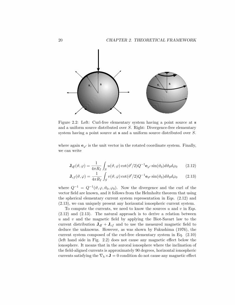
s0s s0
s
Figure 2.2: Left: Curl-free elementary system having a point source at sand a uniform source distributed over S. Right: Divergence-free elementarysystem having a point source at s and a uniform source distributed over S.
where again eϕ′ is the unit vector in the rotated coordinate system. Finally,we can write
Jdf (ϑ, ϕ) =1
4πRI
∫S
u(ϑ, ϕ) cot(ϑ′/2)Q−1eϕ′ sin(ϑ0)dϑ0dϕ0 (2.12)
Jcf (ϑ, ϕ) =1
4πRI
∫S
v(ϑ, ϕ) cot(ϑ′/2)Q−1eϑ′ sin(ϑ0)dϑ0dϕ0 (2.13)
where Q−1 = Q−1(ϑ, ϕ, ϑ0, ϕ0). Now the divergence and the curl of thevector field are known, and it follows from the Helmholtz theorem that usingthe spherical elementary current system representation in Eqs. (2.12) and(2.13), we can uniquely present any horizontal ionospheric current system.
To compute the currents, we need to know the sources u and v in Eqs.(2.12) and (2.13). The natural approach is to derive a relation betweenu and v and the magnetic field by applying the Biot-Savart law to thecurrent distribution Jdf + Jcf and to use the measured magnetic field todeduce the unknowns. However, as was shown by Fukushima (1976), thecurrent system composed of the curl-free elementary system in Eq. (2.10)(left hand side in Fig. 2.2) does not cause any magnetic effect below theionosphere. It means that in the auroral ionosphere where the inclination ofthe field-aligned currents is approximately 90 degrees, horizontal ionosphericcurrents satisfying the∇h×J = 0 condition do not cause any magnetic effect
21
on the ground. Further, it is shown in Paper V that the divergence-freeelementary systems can fully explain the ground magnetic field variationscaused by any three-dimensional ionospheric current system, independentof the inclination of the field-aligned currents. This is the ultimate reasonwhy the divergence-free elementary currents are just equivalent currents(Jdf = Jeq). The complete three-dimensional current system cannot bededuced from the ground magnetic field only. Note that also the curl-freepart of the currents can be deduced if the field-aligned current density (givingv(ϑ, ϕ)) is known (Amm, 2001).
It follows from the discussion above, that we only need the divergence-free elementary systems in this work. The vector potential related to Gel
df (ϑ′)in Eq. (2.11) with the source u0 at ϑ′ = 0 can be computed from
A(s′) =µ0u0
16π2RI
∫S
cot(ϑ′0/2)|s′ − s′0|
eϕ′ds′0 (2.14)
where s′ is now a vector on a spherical shell having radius r < RI . Integral(2.14) can be calculated by expanding the denominator using the additiontheorem for Legendre functions and by eliminating the resulting series (seethe details from the Appendix of Amm and Viljanen, 1999). The magneticfield of the elementary system in the polar coordinate system with pole ats0 is obtained as ∇×A and can be expressed as
Bϑ′ = − µ0u0
4πr sin(ϑ′)
rRI− cos(ϑ
′)√
1− 2r cos(ϑ′)
RI+(
rRI
)2+ cos(ϑ
′)
(2.15)
Br′ = −µ0u0
4πr
1√1− 2r cos(ϑ′ )
RI+(
rRI
)2− 1
(2.16)
where Bϑ′ = B · eϑ′ and Br′ = B · er′ . Eqs. (2.15) and (2.16) express therelation between the source u and the magnetic field B. We thus can find Jdf
in Eq. (2.12). Note that Eqs. (2.15) and (2.16) can be used to express themagnetic field in a continuum analogously to Eq. (2.12). The correspondingexpression is the one for which the discretization is made below.
To look at the computation of the source u in practical applications, wefirst define a scaling factor I for the gridpoint of area A as
I =∫
Au(ϑ0, ϕ0) sin(ϑ0)dϑ0dϕ0 (2.17)
22 CHAPTER 2. THEORETICAL FRAMEWORK
Then, using a discrete elementary system grid, we can write for the magneticfield at the surface of the Earth
B(ϑ, ϕ) =M∑
j=1
IjTjdf (ϑ, ϕ) (2.18)
where Tjdf are the geometric parts of Eqs. (2.15) and (2.16) (u0 omitted)
with r = Re (radius of the Earth) for M divergence-free elementary systemshaving poles at (ϑj , ϕj). Rotations to a common coordinate system usingthe operator Q−1 are not written here explicitly. By expanding Relation(2.18) for a discrete set of N measurements of the ground magnetic field atthe locations (ϑi, ϕi) we obtain the following set of equations
Bϑ(ϑ1, ϕ1)Bϕ(ϑ1, ϕ1)Br(ϑ1, ϕ1)
...Bϑ(ϑN , ϕN )Bϕ(ϑN , ϕN )Br(ϑN , ϕN )
=
T 1ϑ(ϑ1, ϕ1) ... TM
ϑ (ϑ1, ϕ1)T 1
ϕ(ϑ1, ϕ1) ... TMϕ (ϑ1, ϕ1)
T 1r (ϑ1, ϕ1) ... TM
r (ϑ1, ϕ1)...
...T 1
ϑ(ϑN , ϕN ) ... TMϑ (ϑN , ϕN )
T 1ϕ(ϑN , ϕN ) ... TM
ϕ (ϑN , ϕN )T 1
r (ϑN , ϕN ) ... TMr (ϑN , ϕN )
I1...
IM
(2.19)
where on the left hand side we have the measured and on the right hand sidethe modeled field. The solution to (2.19) is obtained by finding the set ofscaling factors I = (I1 . . . IM )T that reproduce the measured magnetic field.Due to the the usually under-determined character of the problem, i.e. M >N , a direct solution for example by means of normal equations would leadto numerical instabilities. Therefore, we use singular value decomposition(SVD). SVD stabilizes the least squares solution by searching the linearcombination of solutions providing the smallest |I|2. Without going intofurther details, we note that in practice the stabilization in SVD is made bychoosing the threshold ε for singular values related to different basis vectorsof the decomposition. A larger value of ε implies a larger number of rejectedbasis vectors and in general a smoother solution for I. For more details onSVD see Press et al. (1992, pp. 51-63). When I, i.e u’s in terms of Relation(2.17), from Eq. (2.19) has been obtained, we are able to compute thedivergence-free equivalent currents anywhere in the ionospheric plane. Notethat the treatment can be given similarly also for the Cartesian geometry(see Amm, 1997). The resulting mathematical expressions are somewhatsimpler in the Cartesian case, but due to the application of the SECS method
23
also to global problems (e.g., Huttunen et al., 2002), a treatment in sphericalgeometry was given here.
The magnetic disturbance caused by electromagnetic induction in theEarth is usually neglected in ionospheric studies. This leads to an over-estimation of the current amplitudes (Viljanen et al., 1995; Tanskanen etal., 2001) but the overall pattern of ionospheric equivalent currents is notseverely miscalculated. However, some care about induction effects is neededwhen the SECS method is applied. If we set elementary currents only inthe ionosphere, we implicitly assume that the disturbance field is purely ofexternal origin. Because this is not exactly true, we do not solve the currentamplitudes by using all three components of the ground magnetic field, butwe only use horizontal components. This is acceptable, because the hori-zontal field can always be explained by using a purely ionospheric source (oras well, by a purely internal source). For a more detailed discussion on thismatter see Paper III. The effect of induction is neglected in Papers III andIV (discussed in Chapter 3) where only the overall ionospheric equivalentcurrent patterns are of interest and thus the full treatment of induction isnot required. However, in Paper V, the SECS method is applied in a mannerwhere also induction effects are taken into account. This will be discussedin Section 2.1.1.
To complete our discussion, we present the explicit form of the operatorQ(ϑ, ϕ, ϑ0, ϕ0) carrying out the coordinate transformations (rotations) inEqs. (2.12) and (2.13). Q is defined as er′
eϑ′
eϕ′
= Q
er
eϑ
eϕ
(2.20)
Q is composed of two operators Trot and Tsc:
Q = T−1sc (ϑ′, ϕ′)Trot(ϑ0, ϕ0)Tsc(ϑ, ϕ) (2.21)
where Tsc carry out the transformations between the spherical and the Carte-sian coordinate systems and Trot carries out the rotation of the coordinatesystem in the Cartesian coordinates. When using the standard relation be-tween the coordinate systems, Tsc can be written as
Tsc =
sin(ϑ) cos(ϕ) cos(ϑ) cos(ϕ) − sin(ϕ)sin(ϑ) sin(ϕ) cos(ϑ) sin(ϕ) cos(ϕ)
cos(ϑ) − sin(ϑ) 0
(2.22)
where (ϑ, ϕ) denotes the polar and azimuth angle of the point in the oldcoordinate system. Due to orthogonality of the transformations T−1
sc = T Tsc,

24 CHAPTER 2. THEORETICAL FRAMEWORK
and (ϑ′, ϕ′) in T−1sc denotes the polar and azimuth angle of the point in the
rotated coordinate system. Trot can be written as
Trot =
cos(ϕ0) sin(ϕ0) 0− cos(ϑ0) sin(ϕ0) cos(ϑ0) cos(ϕ0) − sin(ϑ0)− sin(ϑ0) sin(ϕ0) sin(ϑ0) cos(ϕ0) cos(ϑ0)
(2.23)
where ϑ0 and ϕ0 are polar and azimuthal angles of the rotation. Note theorder of the rotation: 1.) ϕ0 is made counter-clockwise keeping the z-axisconstant and 2.) ϑ0 is made clockwise keeping the rotated x-axis constant.Now angles (ϑ′, ϕ′) needed in T−1
sc can be obtained by first computing x′
y′
z′
= Trot(ϑ0, ϕ0)Tsc(ϑ, ϕ)
100
(2.24)
and by computing then
ϑ′ = arccosz′√
x′2 + y′2 + z′2(2.25)
ϕ′ = arctany′
x′(2.26)
Some attention should be paid to Eq. (2.26) when choosing the quadrant ofthe inverse tangent. Inverse rotations are carried out by the matrix Q−1 =QT .
2.1.1 Separation of the ground disturbance magnetic fieldinto external and internal parts
This topic is discussed and treated in a complete manner in Paper V. Thusonly a brief discussion about the relation of the field separation to GICstudies together with a very brief introduction to the application of theSECS method to the field separation problem, is given here.
As was noted above, also the magnetic effect arising from electromag-netic induction inside the Earth is contributing to the total field at thesurface, i.e. the ground magnetic field is a superposition of external andinternal parts. In some cases it is acceptable to neglect the internal effects,especially when only an overall behavior of the ionospheric equivalent cur-rent patterns is of interest. However, in some cases neglecting induction may

25
lead to erroneous interpretations or separated field components are neededas a starting point for the entire investigation. For example, dependingon the individual situation, in the analysis of ionospheric electrodynamics,neglecting telluric effects may cause significant errors in the estimation ofthe ionospheric current intensity (Viljanen et al., 1995; Tanskanen et al.,2001), or even notable errors in the determination of some global magne-tospheric indices like Dst (Hakkinen et al., 2002). Also, the ratio of theinternal and external components contains information about the underly-ing ground conductivity structure (e.g., Berdichevsky and Zhdanov, 1984,p. 191). Methods applied to the estimation of the Earth’s conductivitystructure require a reliable estimation of the magnetic field spectra for bothcomponents and are thus dependent on an accurate separation.
From the GIC viewpoint, the importance of the field separation is notin the practical modeling of GIC or in understanding the basic ionosphericdynamics. The importance comes forward in the usage of the separatedfields in determining the ground conductivity structure, which is naturallyof a great importance for GIC studies. The separation of the field is alsorequired in the studies where the GIC modeling is made in detail far beyondthe scope of the work presented here. This type of future work is describedin Chapter 4.
The separation of the magnetic disturbance field into external and inter-nal parts is carried out here by utilizing the SECS method. Similarly to theequivalent current determination, there are traditional methods which areused, namely the Gauss-Schmidt (Chapman and Bartels, 1940), the spheri-cal cap harmonics (Haines, 1985), the Fourier (Weaver, 1964; Mersmann etal., 1979) and the spatial (Siebert and Kertz, 1957) method1. The SECSmethod has significant advantages over these methods. The advantagesare basically the computational efficiency and the possibility to make localchoices for the spatial resolution of the determined fields. The idea of theSECS separation is to establish two layers of divergence-free elementary sys-tems, one above the surface of the Earth (r = RI > Re) and another belowit (r = RG < Re). Using the notations of Eq. (2.18), the magnetic field atthe surface of the Earth can be expressed as
B(ϑ, ϕ) =M∑
j=1
IjTjdf (ϑ, ϕ) +
S∑k=1
IkTkdf (ϑ, ϕ) (2.27)
where tilde denotes the scaling factors and geometric parts of the fields1The spatial and the Fourier method are mathematically equivalent via convolution
theorem

26 CHAPTER 2. THEORETICAL FRAMEWORK
corresponding to the internal layer at r = RG. Now for a discrete set of Nmeasurements of the ground magnetic field at locations (ϑi, ϕi) we obtain aset of equations similar to (2.19). The equations can be solved as before inthe least squares sense using SVD. Once I and I are known, the separatedfield components can be computed from Eq. (2.27). Note that again anyground magnetic field variation can be expressed in terms of Eq. (2.27).
2.2 Computation of the ground geoelectric field
Before going into details, let us review some of the basic properties of elec-tromagnetic fields of geomagnetic origin. The mathematics will be discussedin the planar geometry where the standard choice of the coordinate systemin geophysics is utilized (x north, y east, z downward, origin at the sur-face of the Earth). Neglecting the Earth’s curvature is acceptable for localstudies (dimensions less than 1000 km), a requirement that is perfectly ful-filled in this work. The fundamental properties of the fields are expressedby Maxwell’s equations and Ohm’s law:
∇ ·E = ρ/ε (2.28)∇ ·B = 0 (2.29)
∇×E = −∂B∂t
(2.30)
∇×B = µ0j + µ0ε∂E∂t
(2.31)
j = σE (2.32)
where the standard notation is used (see page vii). The media are assumedto be nonmagnetic, i.e. the magnetic permeability of vacuum µ0 = 4π ·10−7 H/m is used. This is a valid and commonly used assumption in allgeomagnetic induction studies.
Taking curl of Eq. (2.30) and using Eqs. (2.31) - (2.32) we obtain
∇2E = ∇(∇ ·E) + µ0σ∂E∂t
+ µ0ε∂2E∂t2
(2.33)
Following the treatment by Weaver (1994), we define a dimensionless pa-rameter t′ = t/T where T is the characteristic time of the phenomena underinvestigation. Substituting t′ into Eq. (2.33), we obtain
∇2E = ∇(∇ ·E) + κ1∂E∂t′
+ κ2∂2E∂t′2
(2.34)
27
where κ1 = µ0σ/T and κ2 = µ0ε/T 2. When the smallest time scales ofinterest (1 s) and the lowest estimate for a possible ground conductivity (or-der of 10−5 S/m) and the vacuum value for the permittivity ε are chosen wefind that κ1/κ2 = σT/ε0 is of the order of 108, i.e. κ1 � κ2. Consequently,the last term in Eq. (2.34) can be neglected. This is the so-called quasi-stationary approximation which is generally valid for all geomagnetic induc-tion applications. The quasi-static approximation is equivalent to neglectingthe last term in Eq. (2.31), i.e the displacement current. By applying theapproximation, we see from Eq. (2.31) that ∇ · j = 0, i.e. the current inthe Earth is divergence-free. The divergence-free condition applied to Eq.(2.32) gives
(∇σ) ·E + σ∇ ·E = 0 (2.35)
By solving ∇ · E from this expression and substituting into the quasi-stationary version of Eq. (2.33) we obtain
∇2E = −∇((∇σ) ·E/σ) + µ0σ∂E∂t
(2.36)
A significant simplification of Eq. (2.36) is obtained if gradients of theconductivity can be neglected. A common way to do this is to use a blockmodel of the Earth where the conductivity is uniform within each block.This is valid in regions where geological structures rather than temperaturegradients cause variations of the conductivity. Usually in GIC studies, theEarth conductivity structure is assumed to be locally either one-dimensional(conductivity blocks just in the z direction), i.e. layered, or completelyuniform. These are the assumptions used also in this work. If ∇σ = 0 Eq.(2.36) takes the form
∇2E = µ0σ∂E∂t
(2.37)
which is the vector diffusion equation for the electric field. Noteworthy isthat due to the neglected displacement currents Eq. (2.37) describes a fieldthat is behaving diffusively in the medium rather than propagating as anelectromagnetic wave. Furthermore, it is an easy task to show that also themagnetic field field satisfies the diffusion equation in a uniform conductor
∇2B = µ0σ∂B∂t
(2.38)
The diffusion equations with boundary conditions for the electromagneticfields form the basis for the standard treatment of the geomagnetic induction

28 CHAPTER 2. THEORETICAL FRAMEWORK
problem (see e.g., Weaver, 1994).It is also worth noting that due to the very small conductivity of the air
(order of 10−14 S/m), there is in practice no galvanic connection between theEarth and ionospheric or magnetospheric current sources. It follows, thatthe electromagnetic field in the Earth is of inductive origin. Furthermore,if there are no horizontal variations in the Earth’s conductivity, the electricfield inside the Earth is always horizontal, i.e. the vertical component Ez
is always zero. This is seen by using the boundary condition of the currentdensity
σ1E1 · n = σ2E2 · n (2.39)
where n is the unit vector normal to the boundary. This follows from the∇ · j = 0 condition. If the conductivity of the air is taken to be zero, itfollows from (2.39) that the vertical component of electric field right belowthe surface must be zero. If also at the bottom layer, or at z → ∞, thevertical field is zero, it follows that the only solution of Eq. (2.37) for thevertical component is Ez = 0 inside the Earth, i.e. the electric field ishorizontal.
2.2.1 Computation via surface magnetic field
From the viewpoint of the study at hand, it is of great interest to know therelation between the variations of the ground magnetic field and the horizon-tal geoelectric field E(x,y)(z = 0) driving GIC. Contrary to the geoelectricfield measurements, good quality ground magnetic field data are availablefrom numerous stations distributed throughout the world, and long timeseries are available. Thus, it is clear that the ground geomagnetic field is akey quantity for the GIC modeling.
Let us start from Eq. (2.37). Express B = (Bx, By, Bz) and E =(Ex, Ey, Ez) as Fourier integrals
B(x, y, z, t) =1
(2π)3/2
∫ ∫ ∫ ∞−∞
b(α, β, z, ω)ei(αx+βy+ωt)dαdβdω (2.40)
E(x, y, z, t) =1
(2π)3/2
∫ ∫ ∫ ∞−∞
e(α, β, z, ω)ei(αx+βy+ωt)dαdβdω (2.41)
where b = (bx, by, bz) and e = (ex, ey, ez). Then Eq. (2.37) reduces to
∂2e∂z2
− γ2e = 0 (2.42)

29
where γ2 = α2 + β2 + iωµ0σ. The solution of Eq. (2.42) for horizontalcomponents can be expressed as
e(x,y)(z) = c(x,y)eγz + d(x,y)e
−γz (2.43)
where c and d are complex values and we choose Re(γ) > 0.2 From Eq.(2.30), using Eqs. (2.40) and (2.41) and utilizing the fact that Ez = 0 insidethe Earth, we obtain
∂ey
∂z= iωbx (2.44)
∂ex
∂z= −iωby (2.45)
βex − αey = ωbz (2.46)
The task is to find the relation between the horizontal components ofthe magnetic field and the geoelectric field at the surface of the Earth. Letus define the spectral impedance as
Z = µ0ex
by= −µ0
ey
bx(2.47)
Where the last equality can be verified using conditions [∇ × B]z = 0 and∇h · E = 0 which follow from the Ez = 0 condition. Using Eq. (2.43) andRelations (2.44) and (2.45) we obtain
Z = − iωµ0
γ
c(x,y)eγz + d(x,y)e
−γz
c(x,y)eγz − d(x,y)e−γz(2.48)
which can be rewritten as
Z = − iωµ0
γcoth(γz + s) (2.49)
where s = ln(√
c(x,y)/d(x,y)).Eq. (2.49) is valid for a uniform conductor. Next we consider a layered
Earth structure. Now with γ2 → γ2n = α2 +β2 + iωµ0σn and s → sn at layer
zn ≤ z ≤ zn+1 we can write (2.49) at the bottom of the layer (z = zn+1) as
Z(zn+1) = − iωµ0
γncoth(γnzn+1 + sn) (2.50)
2The same convention is applied henceforth for all square roots of complex numbers

30 CHAPTER 2. THEORETICAL FRAMEWORK
and at the top of the layer (z = zn) as
Z(zn) = − iωµ0
γncoth(γnzn + sn) (2.51)
By eliminating sn from these expressions we obtain a recursive formula
Z(zn) =iωµ0
γncoth(γndn + coth−1(
γn
iωµ0Z(zn+1))) (2.52)
where dn = zn+1−zn. Eq. (2.52) is known as Lipskaya formula (Berdichevskyand Zhdanov, 1984, p. 53) and it determines the spectral impedance at thetop of the nth layer in terms of the impedance at the bottom of the layer.In general the impedance is dependent on the frequency and also on thewavenumbers α and β. To obtain the surface impedance Z0, one just setsn = 1 in Eq. (2.52) and computes the impedance values recursively startingfrom the bottom of the modeled Earth structure.
Let us then investigate in greater detail Relation (2.47). First we moveback into the spatio-temporal domain. Using (2.41) we obtain
E0(x,y)(x, y, t) =
1(2π)3/2
∫ ∫ ∫ ∞−∞
e0(x,y)e
i(αx+βy+ωt)dαdβdω
= ± 1(2π)3/2µ0
∫ ∫ ∫ ∞−∞
Z0b0(y,x)e
i(αx+βy+ωt)dαdβdω (2.53)
where the subscript 0 denotes the corresponding quantities at the surfaceof the Earth (z = 0). Concentrating here just on the x-component (they-component is handled identically) and applying the convolution theoremto Eq. (2.53), we obtain
E0x(x, y, t) =
1(2π)3/2µ0
∫ ∫ ∫ ∞−∞
G(x′, y′, t′)0B0y(x−x′, y−y′, t−t′)dx′dy′dt′
(2.54)where the kernel of the integral is defined as
G(x′, y′, t′)0 =1
(2π)3/2
∫ ∫ ∫ ∞−∞
Z0ei(αx′+βy′+ωt′)dαdβdω (2.55)
Consequently, if we are able to evaluate the integral in (2.55), we can trans-form the horizontal magnetic field measured at the Earth’s surface into thehorizontal geoelectric field via Eq. (2.54). However, one usually does not

31
know the magnetic field from very large (infinite) area and over very longtime intervals and thus some approximations are needed for practical ap-plications. Let us investigate, in the fashion of Dmitriev and Berdichevsky(1979), the basic properties of G(x′, y′, t′)0 in the case of a uniform groundconductivity structure. By setting dn equal to infinite in Eq. (2.52), weobtain
G(x′, y′, t′)0 =iµ0
(2π)3/2
∫ ∫ ∫ ∞−∞
ω
γnei(αx′+βy′+ωt′)dαdβdω (2.56)
The spatial part of Eq. (2.56) can be transformed into a Hankel integral(e.g., Arfken and Weber, 1995, p. 849)
G(r′, t′)0 =iµ0√2π
∫ ∞−∞
∫ ∞0
ω√ρ2 + k2
ρJ0(r′ρ)eiωt′dρdω (2.57)
where r′ =√
x′2 + y′2, ρ =√
α2 + β2, k2 = iωµσ and J0 is the zeroth orderBessel function. The integration with respect to ρ gives (Gradshteyn andRyzhik, 1965, formula 6.554.1)
G(r′, t′)0 =iµ0√2π
∫ ∞−∞
ωe−kr′
r′eiωt′dω (2.58)
Before proceeding it is noted that the quasi-static approximation has beenused, i.e. σT/ε was assumed to be large. This is strictly valid for all temporalvariations only if σ/ε approaches infinity. However, the highest frequenciesof the relevant geomagnetic variations observable on the ground rarely ex-ceed 1 Hz and thus in practice the quasi-static approximation holds for alltemporal variations of geomagnetic origin (see e.g., Keller and Frischknecht,1970, p. 200). We seek for a pragmatic approach and thus we assume thatthe contribution from the frequencies above the validity of the quasi-staticapproximation to the b0
(x,y) term of Eq. (2.53) are negligible. Consequently,it is reasonable to carry out the integration in Eq. (2.58) from −∞ to ∞since the frequencies for which the approximation is not valid, do not con-tribute to the final geoelectric field (see also discussion by Pirjola, 1982, p.20-25). Let us then investigate the causality. By making a substitution√
ω = κ, the integral (including only terms contributing to the integral)appearing in Eq. (2.58) can be written as
2∫ ∞0
κ3e−cκ+iκ2t′dκ− 2∫ ∞0
κ3eicκ−iκ2t′dκ (2.59)
32 CHAPTER 2. THEORETICAL FRAMEWORK
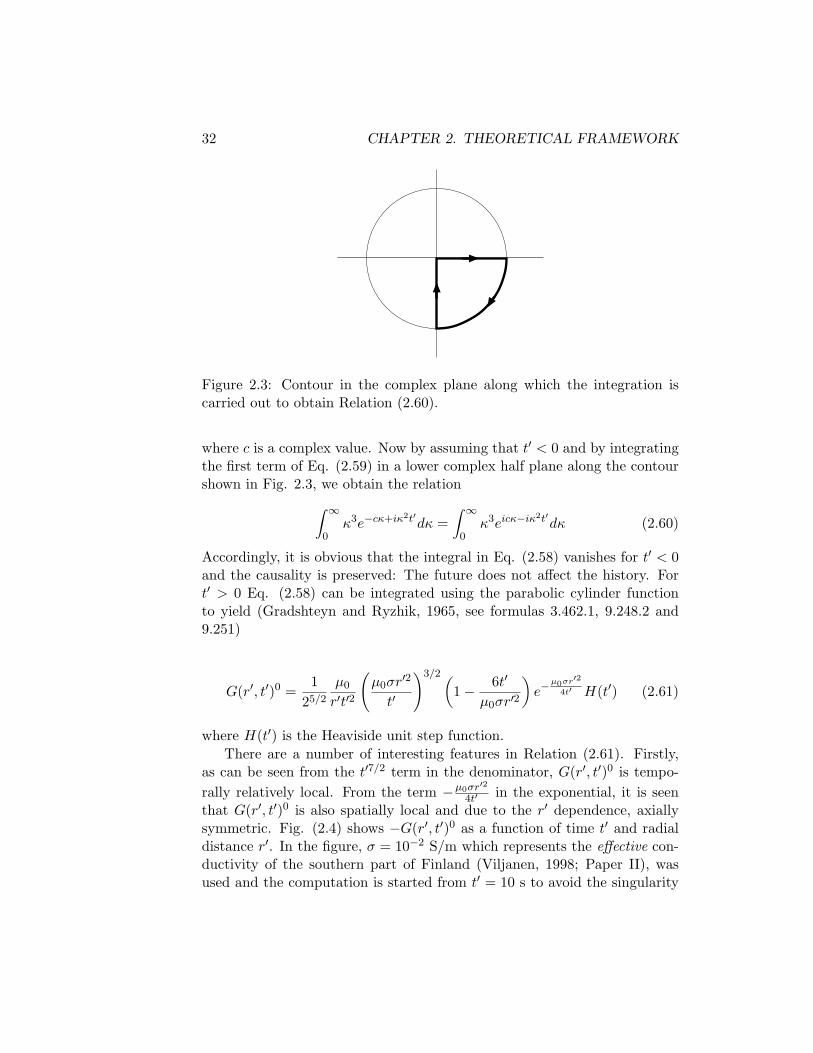
Figure 2.3: Contour in the complex plane along which the integration iscarried out to obtain Relation (2.60).
where c is a complex value. Now by assuming that t′ < 0 and by integratingthe first term of Eq. (2.59) in a lower complex half plane along the contourshown in Fig. 2.3, we obtain the relation∫ ∞
0κ3e−cκ+iκ2t′dκ =
∫ ∞0
κ3eicκ−iκ2t′dκ (2.60)
Accordingly, it is obvious that the integral in Eq. (2.58) vanishes for t′ < 0and the causality is preserved: The future does not affect the history. Fort′ > 0 Eq. (2.58) can be integrated using the parabolic cylinder functionto yield (Gradshteyn and Ryzhik, 1965, see formulas 3.462.1, 9.248.2 and9.251)
G(r′, t′)0 =1
25/2
µ0
r′t′2
(µ0σr′2
t′
)3/2 (1− 6t′
µ0σr′2
)e−
µ0σr′2
4t′ H(t′) (2.61)
where H(t′) is the Heaviside unit step function.There are a number of interesting features in Relation (2.61). Firstly,
as can be seen from the t′7/2 term in the denominator, G(r′, t′)0 is tempo-rally relatively local. From the term −µ0σr′2
4t′ in the exponential, it is seenthat G(r′, t′)0 is also spatially local and due to the r′ dependence, axiallysymmetric. Fig. (2.4) shows −G(r′, t′)0 as a function of time t′ and radialdistance r′. In the figure, σ = 10−2 S/m which represents the effective con-ductivity of the southern part of Finland (Viljanen, 1998; Paper II), wasused and the computation is started from t′ = 10 s to avoid the singularity

33
050
100150
200
1020
3040
5060
0
1
2
3
4
5
6
x 10-13
r´ [km]t´ [s]
Figure 2.4: Temporal and spatial behavior of −G(r′, t′)0 in Eq. (2.61).σ = 10−2 S/m has been used in computing the values. The diamondsdenote the values r′s =
√4t′
µ0σ .
at the origin. As it is seen from the figure, the main contribution to G(r′, t′)0
comes from the vicinity of the origin. The decay to 1/e is obtained at theradius r′s =
√4t′
µ0σ . With the chosen Earth parameters this is less than 150km for t′ = 60 s. Thus it is obvious that for obtaining the effective valuesfor E0
x(x, y, t) in Eq. (2.54), we do not need information about the groundmagnetic field variations from distances of several hundreds of kilometers.Furthermore, if we may assume that the spatial magnetic field variationswithin the effective radius of G(r′, t′)0 are linear, we need only one measure-ment point of the magnetic field to compute the local effective geoelectricfield E0
x(x, y, t). This is due to axial symmetry of G(r′, t′)0 and is easily seenby substituting
B0y(x− x′, y − y′, t− t′) = B0
y(x, y, t− t′) + ax′ + by′
= B0y(x, y, t− t′) + ar′ cos(φ′) + br′ sin(φ′) (2.62)
where a and b are just some constants and where the transformation to
34 CHAPTER 2. THEORETICAL FRAMEWORK
cylindrical coordinates has been made. In cylindrical coordinates Eq. (2.54)becomes
E0x(x, y, t) =
1(2π)3/2µ0
∫ ∞0
∫ 2π
0
∫ ∞0
G(r′, t′)0[B0y(x, y, t− t′) +
ar′ cos(φ′) + br′ sin(φ′)]r′dr′dφ′dt′
=1√
2πµ0
∫ ∞0
∫ ∞0
G(r′, t′)0B0y(x, y, t− t′)r′dr′dt′ (2.63)
where the r′ dependence is found only in G(r′, t′)0 and thus the magneticfield is needed only at point (x, y). Let us now assume spatially linearmagnetic field variations and substitute (2.61) to (2.63). From this, ther′ dependence is eliminated by integration (Gradshteyn and Ryzhik, 1965,formula 3.461.3) and we obtain
E0x(x, y, t) = − 1
2√
πµ0σ
∫ ∞0
B0y(x, y, t− t′)
t′3/2dt′ (2.64)
This can be further modified by integrating by parts. We get
E0x(x, y, t) = − 1
√πµ0σ
∫ ∞0
g0y(x, y, t− t′)
√t′
dt′ (2.65)
where g0y = dB0
y/dt′. And finally, this can be written as
E0x(x, y, t) =
1√
πµ0σ
∫ t
−∞
g0y(x, y, t′)√
t− t′dt′ (2.66)
Identically, for the Ey-component we obtain
E0y(x, y, t) = − 1
√πµ0σ
∫ t
−∞
g0x(x, y, t′)√
t− t′dt′ (2.67)
Well known Relations (2.66)-(2.67) are identical to those that would havebeen obtained by assuming the source field to be a downward propagatingplane wave, the assumption forming the basis of the magnetotelluric sound-ing method (Cagniard, 1953). However, as was seen above, the plane waverequirement can be relaxed to assumptions about the locally (∼ 100 km)linear behavior of the surface magnetic variations. This is a result thatsimplifies the practical GIC modeling significantly. To estimate the localgeoelectric field behavior we need geomagnetic recordings only from onesingle point.
35
Above the uniform ground condctivity was employed. For layered Earthconductivity structures the situation becomes more difficult. Anyhow, themain conclusions above hold for typical conductivity structures (Dmitrievand Berdichevsky, 1979). An approach for modeling a multilayered Earthis to use Eq. (2.52) with α and β equal to zero (plane wave) and computingthe surface impedance using the known conductivities of the layers. Thecomputation of the electric field is made in the frequency domain via Eqs.(2.47) and the time domain field is obtained by Fourier transforms. However,although the multilayered approach is in principle more exact, it has beenseen in numerous investigations that in practice Eqs. (2.66)-(2.67), appliedwith some effective conductivity estimate exhibiting the average behavior ofthe fields with relevant periods, are able to give the surface geoelectric fieldwith an accuracy sufficient for GIC modeling (e.g., Viljanen and Pirjola,1989; Viljanen, 1998; Paper I). The main requirement is that the magneticdata used is from the vicinity of the GIC-modeling region. Also, Relations(2.66)-(2.67) are directly applicable to real-time computations.
Worth noting here is that Relations (2.66)-(2.67) suggest that there isa close connection between the time derivative of the horizontal magneticfield and the horizontal surface geoelectric field, i.e. dBx,y/dt ∼ Ey,x. Con-sequently, the time derivative of the horizontal magnetic field is a good in-dicator for GIC activity (Viljanen et al., 2001). This feature will be utilizedin Chapter 3.
2.2.2 Computation using a known ionospheric current sys-tem
If, instead of ground magnetic field variations, the ionospheric current sys-tem is known, another pragmatic approach can be used for GIC-relatedgeoelectric field computations. The method is based on the complex im-age representation of the ground induction contribution and it simplifies theequations for the total electromagnetic field at the surface of the Earth sig-nificantly. The fundamental idea behind the complex image method (CIM)was presented by Wait and Spies (1969) and is reviewed below.
Let us again assume a homogeneous Earth with the conductivity σ, zeroair conductivity and a horizontal ionospheric source current (see Fig. 2.5).Any three-dimensional ionospheric source current can be equivalently rep-resented by a horizontal current distribution, as was shown in Section 2.1.Horizontal ionospheric currents do not produce a vertical electric field, thusalso the primary component, i.e. the field in the absence of the conductingEarth, Ep
z = 0. The x-component of the electric field in the region between

36 CHAPTER 2. THEORETICAL FRAMEWORK
the surface of the Earth and ionosphere (−h < z ≤ 0) and in the Earth(z ≥ 0) can be expressed using Eq. (2.43) with the boundary conditione1x(∞) = 0
e0x(z) = c0
xeγ0z + epx(0)e−γ0z, −h < z ≤ 0 (2.68)e1x(z) = d1
xe−γ1z, z ≥ 0 (2.69)
where epx(0) is the spectrum (α, β, ω) of the x-component of the primary
electric field at the surface. The continuity of by and ex across the boundaryz = 0 with Relation (2.45) implies
c0x + ep
x(0) = d1x (2.70)
γ0c0x − γ0e
px(0) = −γ1d
1x (2.71)
from which c0x can be solved and Eq. (2.68) takes the form
e0x(z) =
γ0 − γ1
γ0 + γ1epx(0)eγ0z + ep
x(0)e−γ0z (2.72)
where the first term on the right-hand side represents the secondary fieldarising from induction in the Earth (denoted below by e0,ind
x (z)). Let ustake a closer look at this term. We multiply the term by eγ02pe−γ02p, i.e. byone. p is so far an arbitrary parameter and is not to be confused with theprimary component of the electric field. One obtains
e0,indx (z) =
γ0 − γ1
γ0 + γ1eγ02pep
x(0)eγ0(z−2p) = K(η)epx(0)eγ0(z−2p) (2.73)
where we have defined α2 + β2 = η2. Accordingly, γ0 = η and γ1 =√η2 + iωµ0σ. Next we define
p = limη→0
Z0
iωµ0(2.74)
where Z0(η = 0) is the surface impedance, given by Eq. (2.52) with n = 1,for a uniform inducing field (plane wave). Using the chosen definitions weexpand K(η) around η = 0
K(η) =∞∑
n=0
ηn
n!K(n)(0) = −1− η3
3(iωµ0σ)(3/2)+O(η5) (2.75)
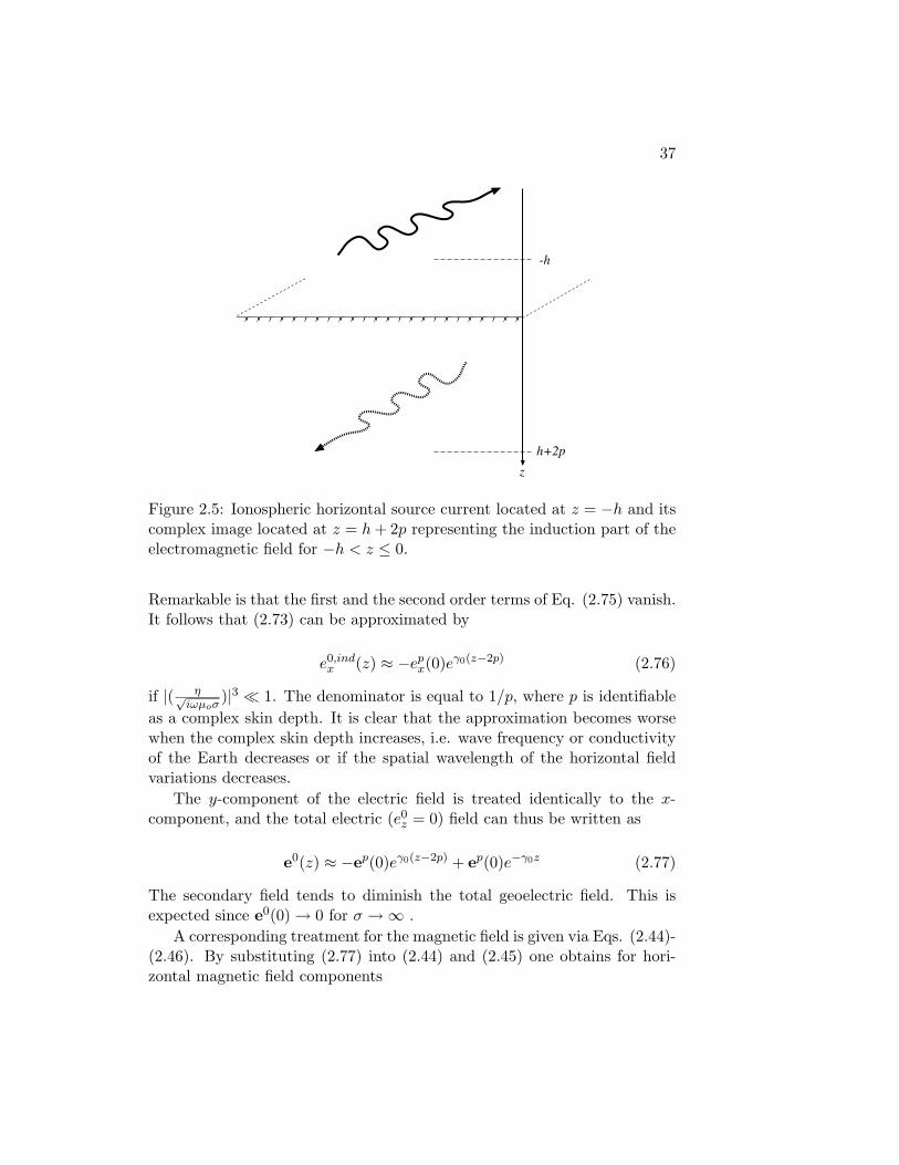
37
-h
z
h+2p
Figure 2.5: Ionospheric horizontal source current located at z = −h and itscomplex image located at z = h + 2p representing the induction part of theelectromagnetic field for −h < z ≤ 0.
Remarkable is that the first and the second order terms of Eq. (2.75) vanish.It follows that (2.73) can be approximated by
e0,indx (z) ≈ −ep
x(0)eγ0(z−2p) (2.76)
if |( η√iωµoσ
)|3 � 1. The denominator is equal to 1/p, where p is identifiableas a complex skin depth. It is clear that the approximation becomes worsewhen the complex skin depth increases, i.e. wave frequency or conductivityof the Earth decreases or if the spatial wavelength of the horizontal fieldvariations decreases.
The y-component of the electric field is treated identically to the x-component, and the total electric (e0
z = 0) field can thus be written as
e0(z) ≈ −ep(0)eγ0(z−2p) + ep(0)e−γ0z (2.77)
The secondary field tends to diminish the total geoelectric field. This isexpected since e0(0) → 0 for σ →∞ .
A corresponding treatment for the magnetic field is given via Eqs. (2.44)-(2.46). By substituting (2.77) into (2.44) and (2.45) one obtains for hori-zontal magnetic field components
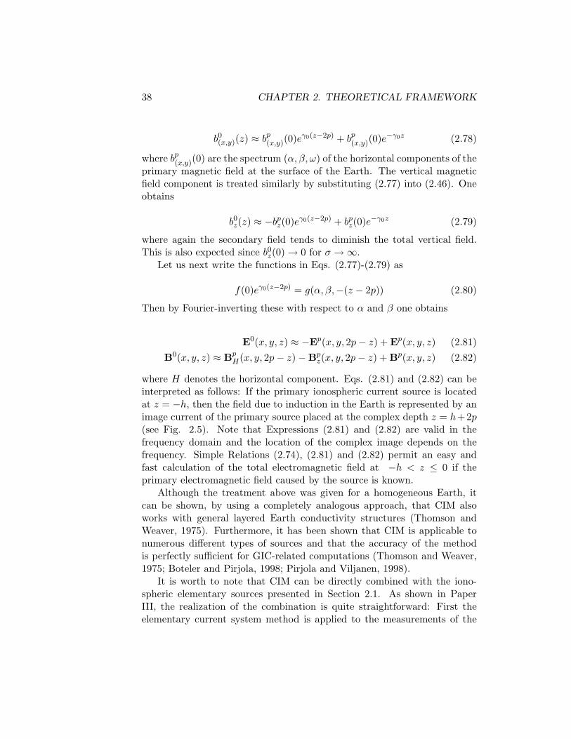
38 CHAPTER 2. THEORETICAL FRAMEWORK
b0(x,y)(z) ≈ bp
(x,y)(0)eγ0(z−2p) + bp(x,y)(0)e−γ0z (2.78)
where bp(x,y)(0) are the spectrum (α, β, ω) of the horizontal components of the
primary magnetic field at the surface of the Earth. The vertical magneticfield component is treated similarly by substituting (2.77) into (2.46). Oneobtains
b0z(z) ≈ −bp
z(0)eγ0(z−2p) + bpz(0)e−γ0z (2.79)
where again the secondary field tends to diminish the total vertical field.This is also expected since b0
z(0) → 0 for σ →∞.Let us next write the functions in Eqs. (2.77)-(2.79) as
f(0)eγ0(z−2p) = g(α, β,−(z − 2p)) (2.80)
Then by Fourier-inverting these with respect to α and β one obtains
E0(x, y, z) ≈ −Ep(x, y, 2p− z) + Ep(x, y, z) (2.81)B0(x, y, z) ≈ Bp
H(x, y, 2p− z)−Bpz(x, y, 2p− z) + Bp(x, y, z) (2.82)
where H denotes the horizontal component. Eqs. (2.81) and (2.82) can beinterpreted as follows: If the primary ionospheric current source is locatedat z = −h, then the field due to induction in the Earth is represented by animage current of the primary source placed at the complex depth z = h+2p(see Fig. 2.5). Note that Expressions (2.81) and (2.82) are valid in thefrequency domain and the location of the complex image depends on thefrequency. Simple Relations (2.74), (2.81) and (2.82) permit an easy andfast calculation of the total electromagnetic field at −h < z ≤ 0 if theprimary electromagnetic field caused by the source is known.
Although the treatment above was given for a homogeneous Earth, itcan be shown, by using a completely analogous approach, that CIM alsoworks with general layered Earth conductivity structures (Thomson andWeaver, 1975). Furthermore, it has been shown that CIM is applicable tonumerous different types of sources and that the accuracy of the methodis perfectly sufficient for GIC-related computations (Thomson and Weaver,1975; Boteler and Pirjola, 1998; Pirjola and Viljanen, 1998).
It is worth to note that CIM can be directly combined with the iono-spheric elementary sources presented in Section 2.1. As shown in PaperIII, the realization of the combination is quite straightforward: First theelementary current system method is applied to the measurements of the
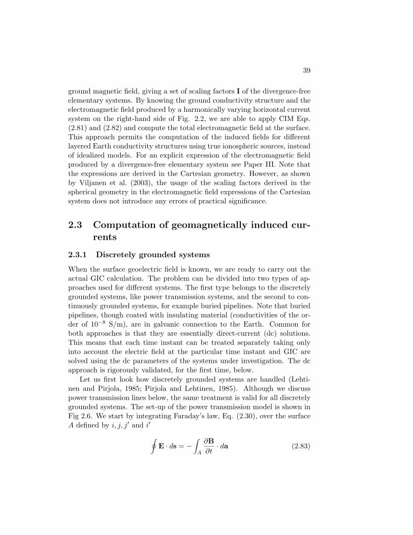
39
ground magnetic field, giving a set of scaling factors I of the divergence-freeelementary systems. By knowing the ground conductivity structure and theelectromagnetic field produced by a harmonically varying horizontal currentsystem on the right-hand side of Fig. 2.2, we are able to apply CIM Eqs.(2.81) and (2.82) and compute the total electromagnetic field at the surface.This approach permits the computation of the induced fields for differentlayered Earth conductivity structures using true ionospheric sources, insteadof idealized models. For an explicit expression of the electromagnetic fieldproduced by a divergence-free elementary system see Paper III. Note thatthe expressions are derived in the Cartesian geometry. However, as shownby Viljanen et al. (2003), the usage of the scaling factors derived in thespherical geometry in the electromagnetic field expressions of the Cartesiansystem does not introduce any errors of practical significance.
2.3 Computation of geomagnetically induced cur-rents
2.3.1 Discretely grounded systems
When the surface geoelectric field is known, we are ready to carry out theactual GIC calculation. The problem can be divided into two types of ap-proaches used for different systems. The first type belongs to the discretelygrounded systems, like power transmission systems, and the second to con-tinuously grounded systems, for example buried pipelines. Note that buriedpipelines, though coated with insulating material (conductivities of the or-der of 10−8 S/m), are in galvanic connection to the Earth. Common forboth approaches is that they are essentially direct-current (dc) solutions.This means that each time instant can be treated separately taking onlyinto account the electric field at the particular time instant and GIC aresolved using the dc parameters of the systems under investigation. The dcapproach is rigorously validated, for the first time, below.
Let us first look how discretely grounded systems are handled (Lehti-nen and Pirjola, 1985; Pirjola and Lehtinen, 1985). Although we discusspower transmission lines below, the same treatment is valid for all discretelygrounded systems. The set-up of the power transmission model is shown inFig 2.6. We start by integrating Faraday’s law, Eq. (2.30), over the surfaceA defined by i, j, j′ and i′∮
E · ds = −∫
A
∂B∂t· da (2.83)
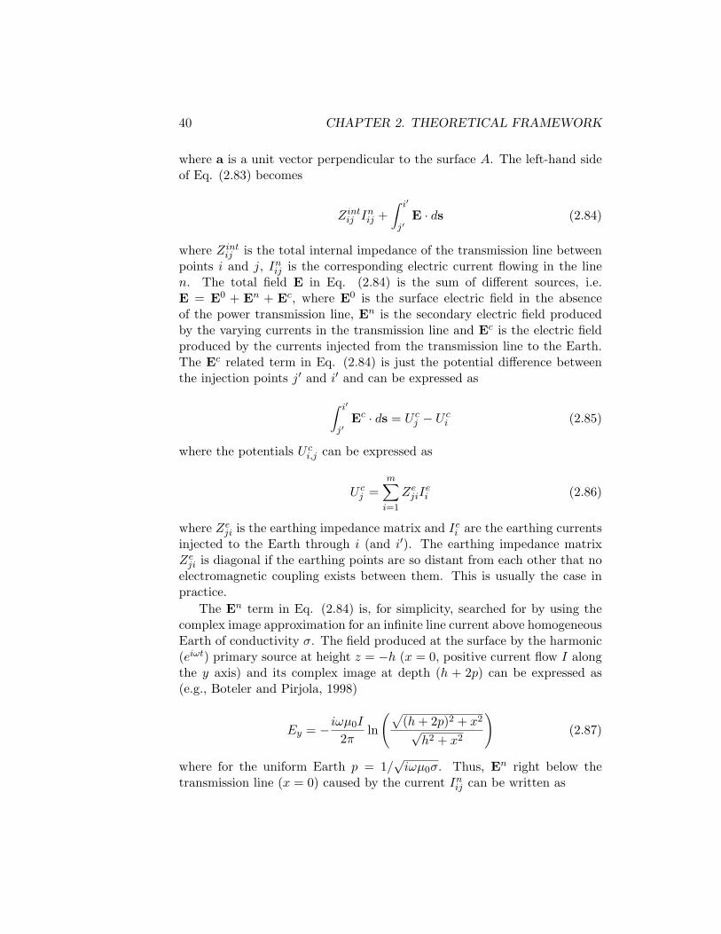
40 CHAPTER 2. THEORETICAL FRAMEWORK
where a is a unit vector perpendicular to the surface A. The left-hand sideof Eq. (2.83) becomes
Zintij In
ij +∫ i′
j′E · ds (2.84)
where Zintij is the total internal impedance of the transmission line between
points i and j, Inij is the corresponding electric current flowing in the line
n. The total field E in Eq. (2.84) is the sum of different sources, i.e.E = E0 + En + Ec, where E0 is the surface electric field in the absenceof the power transmission line, En is the secondary electric field producedby the varying currents in the transmission line and Ec is the electric fieldproduced by the currents injected from the transmission line to the Earth.The Ec related term in Eq. (2.84) is just the potential difference betweenthe injection points j′ and i′ and can be expressed as
∫ i′
j′Ec · ds = U c
j − U ci (2.85)
where the potentials U ci,j can be expressed as
U cj =
m∑i=1
ZejiI
ei (2.86)
where Zeji is the earthing impedance matrix and Ie
i are the earthing currentsinjected to the Earth through i (and i′). The earthing impedance matrixZe
ji is diagonal if the earthing points are so distant from each other that noelectromagnetic coupling exists between them. This is usually the case inpractice.
The En term in Eq. (2.84) is, for simplicity, searched for by using thecomplex image approximation for an infinite line current above homogeneousEarth of conductivity σ. The field produced at the surface by the harmonic(eiωt) primary source at height z = −h (x = 0, positive current flow I alongthe y axis) and its complex image at depth (h + 2p) can be expressed as(e.g., Boteler and Pirjola, 1998)
Ey = − iωµ0I
2πln
(√(h + 2p)2 + x2
√h2 + x2
)(2.87)
where for the uniform Earth p = 1/√
iωµ0σ. Thus, En right below thetransmission line (x = 0) caused by the current In
ij can be written as
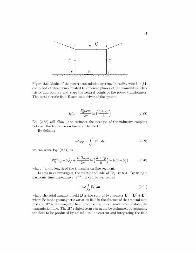
41
Ei’ j’
i jn I nij
I ei I e
j
Figure 2.6: Model of the power transmission system. In reality wire i → j iscomposed of three wires related to different phases of the transmitted elec-tricity and points i and j are the neutral points of the power transformers.The total electric field E acts as a driver of the system.
Enj′i′ =
Inijiωµ0
2πln(
h + 2p
h
)(2.88)
Eq. (2.88) will allow us to estimate the strength of the inductive couplingbetween the transmission line and the Earth.
By defining
−V 0i′j′ =
∫ i′
j′E0 · ds (2.89)
we can write Eq. (2.84) as
Zintij In
ij − V 0i′j′ +
Inijliωµ0
2πln(
h + 2p
h
)− (U c
i − U cj ) (2.90)
where l is the length of the transmission line segment.Let us next investigate the right-hand side of Eq. (2.83). By using a
harmonic time dependence (eiωt), it can be written as
−iω
∫A
B · da (2.91)
where the total magnetic field B is the sum of two sources B = B0 + Bn,where B0 is the geomagnetic variation field in the absence of the transmissionline and Bn is the magnetic field produced by the currents flowing along thetransmission line. The Bn-related term can again be estimated by assumingthe field to be produced by an infinite line current and integrating the field

42 CHAPTER 2. THEORETICAL FRAMEWORK
from the surface of the Earth to the surface of the transmission line. Thisyields
−iω
∫A
Bn · da = −Inijliωµ0
2πln(
h
r0
)(2.92)
where h is the distance from the center of the transmission line wire to thesurface of the Earth and r0 is the radius of the wire.
The B0-related term in Eq. (2.91) can be estimated assuming a planewave source, a uniform Earth and negligible air conductivity. It follows fromEqs. (2.47) and (2.52) that at the surface
bx = −γ1
iωey (2.93)
where γ1 =√
iωµ0σ when α, β → 0. It follows from the condition α, β → 0that there is no x- nor y-dependence in the electromagnetic field, and fromEq. (2.72) with zero air conductivity (γ0 = 0) it follows that above thesurface there is also no z-dependence. Thus, using Relation (2.93) it can bewritten
−iω
∫A
B0 · da = −iω
∫A
B0xda =
h
p
∫ j′
i′E0
yds = −h
pV 0
i′j′ (2.94)
where here p is equal to 1/√
iωµ0σ. If p is defined as in Eq. (2.74), it isclear that (2.94) is generally valid for all layered Earth structures.
Collecting all terms of Eq. (2.83) together we obtain
InijZ
totij − V 0
i′j′(1−h
p)− (U c
i − U cj ) = 0 (2.95)
where
Ztotij = Zint
ij +liωµ0
2πln(
h + 2p
h
)+
liωµ0
2πln(
h
r0
)(2.96)
The internal impedance Zintij can be estimated by using the internal impedance
for an infinite wire per unit length (see e.g., Jordan, 1950, p. 376). One ob-tains
Zintij =
liωµm
2πr0γm
I0(γmr0)I1(γmr0)
(2.97)

43
where the subscript m denotes parameters for the metal of which the wireis composed and I0 and I1 are the zeroth and the first order modified Besselfunctions, respectively.
Now let us investigate the relative importance of different terms in Eq.(2.95). We denote the second term in the right-hand side of Eq. (2.96)by Zind
ij and the last term by Znij . For frequencies below 1 Hz and for a
homogeneous Earth conductivity 10−2 S/m and h = 30 m, the ratio |h/p|is order of 10−3. Thus the corresponding term in Eq. (2.95) can clearly beneglected. Different terms of Eq. (2.96) have been evaluated numericallyfor frequencies from 0 to 1 Hz and are shown in Fig. 2.7. The calculationswere made with µm = 100µ0, σm = 107 S/m, σ = 10−2 S/m, r0 = 0.03 mand h = 30 m, which are realistic values for the present setting. It is seenthat, although the difference at 1 Hz is not any more orders of magnitude,the Zint
ij term dominates for frequencies below 1 Hz. It is also seen that thereal part of Zint
ij is about an order of magnitude larger than the imaginarypart up to 0.1 Hz. Furthermore, the real part remains close to its dc valueat frequencies below 1 Hz.
The above computations indicate that the inductive coupling betweenthe transmission line and the Earth can in practice be neglected, i.e. ourinitial assumption is valid. Furthermore, it was also shown that for themajority of geomagnetic variations, a dc treatment of the GIC flow in atransmission line is justified, although some errors may result from neglect-ing the imaginary part of Zint
ij when approaching frequencies of the order of1 Hz. Consequently, we proceed by approximating Eq. (2.95) as
InijRij − V 0
ij − (U ci − U c
j ) = 0 (2.98)
where Rij is the dc-resistance of the transmission line between points i andj and for convenience we have now marked V 0
i′j′ = V 0ij . Using Kirchhoff’s
law we can write
Iei =
∑j 6=i
Inji = −
∑j 6=i
Inij (2.99)
By substituting Inij in Eq. (2.98) into Eq. (2.99) we obtain
Iei = −
∑j 6=i
V 0ij
Rij−∑j
YijUcj (2.100)
where the network admittance matrix is defined as

44 CHAPTER 2. THEORETICAL FRAMEWORK
0 0.2 0.4 0.6 0.8 10
2
4
6
|Z| [
ohm
]
0 0.2 0.4 0.6 0.8 10
2
4
6
Frequency [Hz]
Z [o
hm]
Figure 2.7: Relative importance of different terms in Eq. (2.96). In the toppanel |Zint
ij | (heavy solid line) |Znij | (dashed line) and |Zind
ij | (thin solid line)for frequencies from 0 to 1 Hz are presented. In the bottom panel the real(solid line) and imaginary (dashed) parts of Zint
ij are shown. See text fordetails.
Yij =
{− 1
Riji 6= j∑
k 6=i1
Riki = j
(2.101)
And finally, using Relation (2.86) we obtain the solution for the earthingcurrent vector
Ie = (1 + YZe)−1Je (2.102)
where
Jei = −
∑j 6=i
V 0ij
Rij(2.103)
Relations (2.86), (2.98) and (2.102) permit the calculation of the currentsanywhere in the transmission system if the electrical parameters Ze
ij , Rij andthe topology of the system and the geoelectric field E0 are known.

45
2.3.2 Continuously grounded systems
The treatment of a continuously grounded systems is quite different fromthe treatment of discretely grounded systems. The details can be found inPaper I and thus only a brief overview is given here. Again, although wediscuss here buried pipelines, the same treatment is valid for all continuouslygrounded systems.
We aim to model pipeline networks. Simplified pipeline models, like aninfinitely long cylinder (see e.g., Ogunade, 1986; Trichtchenko and Boteler,2001) are treated otherwise. The basic idea in modeling a pipeline networkis to represent a segment of the pipeline as a transmission line having asource embedded in it (see Fig. 2 in Paper I). This makes it possible tomodel the pipeline as a distributed source transmission line (DSTL) and touse methods familiar from the transmission line theory (e.g., Smith, 1987).
From the DSTL theory we obtain the following equation describing thecurrent flow I(x) within a uniform pipeline section
d2I(x)dx2
− γ2pI(x) = −YpE0(x) (2.104)
where γp =√
ZpYp and Zp and Yp are the parallel impedance and thetransverse admittance per unit length of the pipeline and are not to beconfused with the spectral impedance treated in Section 2.2 or with theearthing impedance matrix and the network admittance treated in Section2.3.1. γp is effectively the adjustment distance over which discontinuitiesin the pipeline affect the current flow I(x). Similar to discretely groundedsystems, Zp is in practice the dc-resistance of the pipeline metal per unitlength and Yp is the dc-admittance of the pipeline coating (from the pipelinemetal to the ground), thus permitting a dc treatment also for pipelines. Thevalidity of the dc assumption is tested and discussed Paper I. Conclusions areagain similar to those made for discretely grounded systems: For frequenciesof the order of 0.01 Hz or less the dc assumption is perfectly valid, but whenapproaching frequencies of the order of 1 Hz some errors may be introduced ifZp and Yp are kept as dc quantities. However, errors due to the dc treatmentare clearly not large enough to justify the burden of a full ac treatment ofthe problem.
Eq. (2.104) has a simple solution for a single pipeline section. Theprincipal idea in modeling the discontinuities of the pipeline network is tosolve (2.104) for each section separately and to embed the rest of the net-work inside an equivalent terminating impedance and a voltage source, i.e.boundary conditions of the section in question. The equivalent impedance
46 CHAPTER 2. THEORETICAL FRAMEWORK
and the voltage source are computed using the Thevenin theorem (e.g., Fer-ris, 1962). By constructing the boundary conditions one by one recursivelystarting from the ends of the network until the end of the section under con-sideration, we are able to determine the current and the pipe-to-soil voltageprofiles along the entire pipeline network.
2.4 Unification of the methods for practical appli-cations
Here a general method applicable for computation of GIC in technologicalconductor systems on the ground is introduced. It is assumed that magneticfield data from a sufficiently large number of stations is available and thatthe overall ground conductivity structure, the topology of the system andthe electrical dc parameters of the system are known.
Fig. 2.8 presents the flow of different steps of the method. The inputto each model together with the model output are shown. First, the SECSmethod (Section 2.1) is applied to geomagnetic field data from a set ofmeasurements to derive the ionospheric equivalent currents. The ionoshericequivalent currents are then used to compute the magnetic field at any de-sired point at the surface of the Earth. In the next step, the geoelectric fieldis computed using the surface impedance, calculated using the informationfrom the ground conductivity, as described in Section 2.2.1. Finally, thegeoelectric field and the network data is used to compute GIC in any part ofthe conductor system by applying the methods presented in Sections 2.3.1and 2.3.2. Note that the method can be used also for real-time computationsthus permitting nowcasting of GIC.

47
Ground conductivity data
Network data
B(ri,t)Interpolation
(SECS method)B(r,t)
Computation of the electric fieldvia surface impedance
E(r,t)
GIC(r,t)
Computation of GIC
Input Method Output
Figure 2.8: Flow of different steps used in the practical calculation of GICin technological conductor systems on the ground. See text for details.

48 CHAPTER 2. THEORETICAL FRAMEWORK
Chapter 3
Characteristics of intenseGIC events
3.1 Properties of intense meso-scale geoelectricfields
As was seen above, if the electrical parameters and topology of the techno-logical conductor system under investigation and the surface geoelectric fieldare given, we are able to determine GIC in all parts of the system. Thus it isclear that we need to understand the basic nature of the geoelectric field inorder to understand the behavior of GIC. As only large GIC are of interest tous, the main attention is paid to intense geoelectric fields (> 100 mV/km).The reason why we are interested in meso-scale (∼ 100 km) fields is thatdue to integration of the geoelectric field made in calculating (and creating)GIC, formally seen from Eq. (2.89) in Section 2.3 and Eqs. (18) and (19) ofPaper I, small-scale (∼ 1 km) features in the geoelectric field smooth out andare thus not very important from the GIC viewpoint. This is an importantand simplifying feature in GIC studies since the small-scale electric field isvery much dependent on the local conductivity structure which, especiallyin the uppermost layers, can be highly varying. If such regions are takeninto account, the assumption about locally laterally homogeneous conduc-tivity structures used in Section 2.2 would be violated and the modelingof the geoelectric field would become much more complicated. However, itshould be noted that, for example, in the cases of ocean-continent bound-aries and small scale anomalies with very high conductivity contrast to thebackground conductivity, assumption about the lateral homogeneity is soseverely distorted that more sophisticated methods are required for the es-
49
50 CHAPTER 3. CHARACTERISTICS
timation of the GIC-associated geoelectric field.Perhaps the greatest general misconception connected with GIC is the
presumption about the east-west preference of the auroral geoelectric fields.If longitudinally uniform auroral ionospheric currents are assumed to flowonly in the east-west direction and the ground conductivity is laterally uni-form, the assumption is acceptable. However, as shown by Viljanen (1997)and Viljanen et al. (2001), the time derivatives of the ground magnetic field,and thus via Relations (2.66)-(2.67) also the ground geoelectric field, canhave large values in any direction. This means that the source for largetime derivatives is more complicated than just a simple east-west orientedelectrojet. An example of this fact is seen in Fig. 3.1 where the modeled andthe measured GIC in the Finnish pipeline at Mantsala and the time deriva-tive of the north and east components of the ground magnetic field at theNurmijarvi Geophysical Observatory on September 8, 2002 are shown. It isseen that this time GIC closely follows the behavior of the time derivative ofthe east component of the magnetic field (dBy/dt ∼ Ex, see Section 2.2.1),whose magnitude is about twice as large as the magnitude of dBx/dt (∼ Ey).The modeled GIC is computed with the method described in Section 2.3.2and in Paper I.
Having large values of ground geoelectric field to any direction, it isnatural to think that there may be further complications related to the”electrojet-thinking”, namely issues associated with the spatial scales of thesurface geoelectric fields. This has been investigated in Papers III and IV.Again only a brief summary is given here, for details see the attached papers.Looking at the times of large GIC or large time derivatives of the magneticfield, it was shown that the cases studied were imposing various types ofbehavior of the geoelectric field, spatial scales of the fields varying fromthousands of kilometers to less than one hundred kilometers. Patterns ofthe geoelectric fields were also varying to high degree, being dependent onthe type of the ionospheric source. Thus, although spatial scales of about 100km and above are of main interest, already 100 km is a relevant scale forunderstanding the true sources of large GIC. The temporal scales relatedto intense geoelectric fields were seen to be relatively short, varying fromabout 10 minutes down to 1 minute and even less. Thus the periods ofour interest are roughly within the range of 1-600 seconds, longer periodfields are not effective enough, i.e. do not have large enough amplitudes, toproduce notable GIC. This feature is also seen from the example shown inFig. 3.1 where the longest period of the largest GIC is about 600 seconds.
The temporal scales discussed above have important implications for therequirements of the ground conductivity models to be used when computing
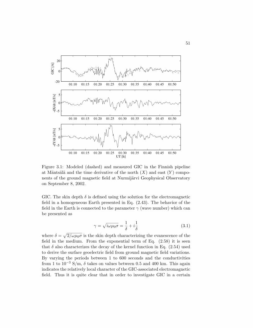
51
01:10 01:15 01:20 01:25 01:30 01:35 01:40 01:45 01:50-20
0
20
GIC
[A]
01:10 01:15 01:20 01:25 01:30 01:35 01:40 01:45 01:50
-5
0
5
-dX
/dt [
nT/s
]
01:10 01:15 01:20 01:25 01:30 01:35 01:40 01:45 01:50
-5
0
5
-dY
/dt [
nT/s
]
UT [h]
Figure 3.1: Modeled (dashed) and measured GIC in the Finnish pipelineat Mantsala and the time derivative of the north (X) and east (Y ) compo-nents of the ground magnetic field at Nurmijarvi Geophysical Observatoryon September 8, 2002.
GIC. The skin depth δ is defined using the solution for the electromagneticfield in a homogeneous Earth presented in Eq. (2.43). The behavior of thefield in the Earth is connected to the parameter γ (wave number) which canbe presented as
γ =√
iωµ0σ =1δ
+ i1δ
(3.1)
where δ =√
2/ωµ0σ is the skin depth characterizing the evanescence of thefield in the medium. From the exponential term of Eq. (2.58) it is seenthat δ also characterizes the decay of the kernel function in Eq. (2.54) usedto derive the surface geoelectric field from ground magnetic field variations.By varying the periods between 1 to 600 seconds and the conductivitiesfrom 1 to 10−3 S/m, δ takes on values between 0.5 and 400 km. This againindicates the relatively local character of the GIC-associated electromagneticfield. Thus it is quite clear that in order to investigate GIC in a certain

52 CHAPTER 3. CHARACTERISTICS
region, meso-scale (∼ 100 km) Earth conductivity models are applicable.This justifies, for example, the approach used in the work by Pulkkinen etal. (2000) where local conductivity models were used to compute the regionalgeoelectric fields via Eqs. (2.66)-(2.67).
On the other hand, small spatial scales of the geoelectric fields at aurorallatitudes indicate that the ground electromagnetic fields or the ionosphericsource cannot be reliably interpolated or extrapolated to great distances,unlike in the case of a one-dimensional electrojet. In order to compute trustworthy GIC estimates, one needs information about the source from theimmediate vicinity of the region of interest. Note that this requirement canpossibly be relaxed at lower latitudes where the source is likely to be moreuniform. For example in the study by Koen (2002), GIC in the SouthernAfrican (mid-latitudes) power transmission system was modeled relativelyaccurately by using ground magnetic data from the Hermanus GeomagneticObservatory located 500 kilometers from the GIC measurement site.
How the discussed properties of the ground geoelectric fields relate toactual GIC has been studied using the methods presented in Chapter 2 forexample by Viljanen et al. (1999), Pulkkinen et al. (2000) and in Paper II. Inthe work of Pulkkinen et al. (2000), GIC in the Finnish power transmissionsystem were studied. In the work, a uniform regional block conductivitymodels of Finland and geomagnetic data from the IMAGE magnetometerarray from the years 1993-1999 were used to calculate the geoelectric fieldvia Eqs. (2.66)-(2.67). The geoelectric field was then used as input to themodel of the transmission system (see Section 2.3.1) giving GIC at differentparts of the system. Fig. (3.2) depicts the distribution of the lengths ofthe peaks during which the sum of the absolute values of GIC through thetransformers of the Finnish high-voltage power system exceeds 400 A. Thedistribution is based on 173 events during which the geomagnetic K index1
at Nurmijarvi Geophysical Observatory reached the value 9. All events lastless than 10 minutes, supporting the conclusions about the relevant periodsmade above. It is also seen that the number of large events is peaked atdurations of less than one minute.
In Fig. 3.3 the geoelectric field pattern and the corresponding GIC in theFinnish power transmission system are shown for an event on April 7, 1995,the time of the snapshot is 16:47 UT. The figure shows a good exampleof the fact that although the spatially small scale features are of a greatimportance, large GIC can be observed throughout the network at the sametime. In this sense, large events exhibit both small and large-scale features,
1three-hour geomagnetic activity index (scale 0-9)
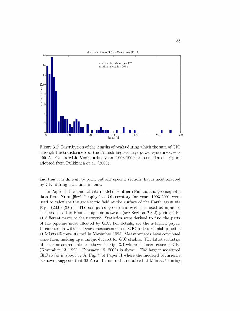
53
0 100 200 300 400 500 6000
2
4
6
8
10
12
14
16
length [s]
num
ber o
f eve
nts
[%]
durations of sum(GIC)>400 A events (K = 9)
total number of events = 173maximum length = 560 s
Figure 3.2: Distribution of the lengths of peaks during which the sum of GICthrough the transformers of the Finnish high-voltage power system exceeds400 A. Events with K=9 during years 1993-1999 are considered. Figureadopted from Pulkkinen et al. (2000).
and thus it is difficult to point out any specific section that is most affectedby GIC during each time instant.
In Paper II, the conductivity model of southern Finland and geomagneticdata from Nurmijarvi Geophysical Observatory for years 1993-2001 wereused to calculate the geoelectric field at the surface of the Earth again viaEqs. (2.66)-(2.67). The computed geoelectric was then used as input tothe model of the Finnish pipeline network (see Section 2.3.2) giving GICat different parts of the network. Statistics were derived to find the partsof the pipeline most affected by GIC. For details, see the attached paper.In connection with this work measurements of GIC in the Finnish pipelineat Mantsala were started in November 1998. Measurements have continuedsince then, making up a unique dataset for GIC studies. The latest statisticsof these measurements are shown in Fig. 3.4 where the occurrence of GIC(November 13, 1998 - February 19, 2003) is shown. The largest measuredGIC so far is about 32 A. Fig. 7 of Paper II where the modeled occurrenceis shown, suggests that 32 A can be more than doubled at Mantsala during

54 CHAPTER 3. CHARACTERISTICS
-600 -400 -200 0 200 400 600 800
-800
-600
-400
-200
0
200
400
max(E) = 7.09 V/kmmax(GIC) = 237 Asum(GIC) = 2351 A
to earthfrom earth
y [km]
x [k
m]
Figure 3.3: Snapshot of geoelectric field (arrows) computed from the groundmagnetic data and the corresponding computed GIC (circle) distributionduring an intense event on April 7, 1995 at 16:47 UT. The radius of thecircle correspond to the magnitude of GIC flowing through the neutrals ofthe power transformers. Figure adopted from Pulkkinen et al. (2000).
the very largest GIC events.
3.2 Properties of ionospheric currents causing in-tense geoelectric fields and the linkage to large-scale magnetospheric phenomena
The primary driver of the geoelectric field in the auroral regions is the iono-spheric electric current system which in turn is connected to the large-scalemagnetospheric and solar wind dynamics (see Fig. 1.2). Thus, the nextnatural step is to look at the ionospheric dynamics related to large GIC,and then ultimately extend this to cover the magnetospheric phenomenain general. These goals demonstrate again quite well the interdisciplinary
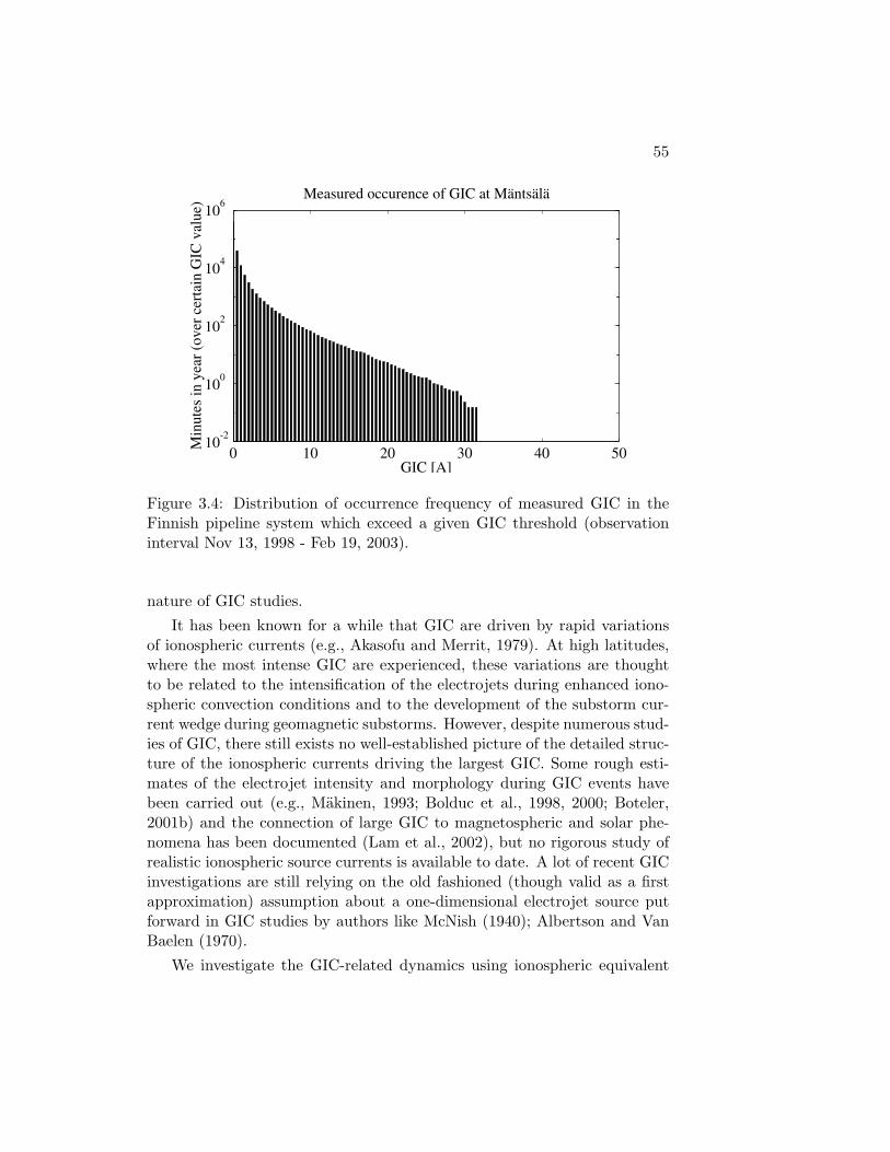
55
0 10 20 30 40 5010-2
100
102
104
106Measured occurence of GIC at Mäntsälä
Min
utes
in y
ear (
over
cer
tain
GIC
val
ue)
GIC [A]
Figure 3.4: Distribution of occurrence frequency of measured GIC in theFinnish pipeline system which exceed a given GIC threshold (observationinterval Nov 13, 1998 - Feb 19, 2003).
nature of GIC studies.
It has been known for a while that GIC are driven by rapid variationsof ionospheric currents (e.g., Akasofu and Merrit, 1979). At high latitudes,where the most intense GIC are experienced, these variations are thoughtto be related to the intensification of the electrojets during enhanced iono-spheric convection conditions and to the development of the substorm cur-rent wedge during geomagnetic substorms. However, despite numerous stud-ies of GIC, there still exists no well-established picture of the detailed struc-ture of the ionospheric currents driving the largest GIC. Some rough esti-mates of the electrojet intensity and morphology during GIC events havebeen carried out (e.g., Makinen, 1993; Bolduc et al., 1998, 2000; Boteler,2001b) and the connection of large GIC to magnetospheric and solar phe-nomena has been documented (Lam et al., 2002), but no rigorous study ofrealistic ionospheric source currents is available to date. A lot of recent GICinvestigations are still relying on the old fashioned (though valid as a firstapproximation) assumption about a one-dimensional electrojet source putforward in GIC studies by authors like McNish (1940); Albertson and VanBaelen (1970).
We investigate the GIC-related dynamics using ionospheric equivalent
56 CHAPTER 3. CHARACTERISTICS
currents which are derived using the spherical elementary current systemmethod as explained in Section 2.1. The approach contains the computa-tion of equivalent currents for periods during which intense induction effectsare experienced, and an investigation of the derived current patterns. Theprimary aim is to shed light on the detailed structure of the source, andultimately to understand the relation to the magnetospheric and solar windconditions. The work has been started in the investigations presented inPapers III and IV. In Paper III, the usage of two-dimensional ionosphericequivalent currents in GIC studies was introduced and ionospheric sourcesfor large geoelectric fields during the disturbed period on June 26, 1998 wereinvestigated. In Paper IV, the same approach was extended to cover the en-tire Sun - solar wind - magnetosphere - ionosphere - ground chain for theApril 6-7, 2000, geomagnetic storm event by using the study by Huttunenet al. (2002) as a background. Findings of these investigations are brieflysummarized and discussed below.
The June 26, 1998, period (01:18 - 01:48 UT) coincided with a substormexpansion phase (on substorms see e.g., Rostoker, 1996; Tanskanen, 2002)during which three different clearly identifiable ionospheric features wereseen to cause intense geoelectric fields. These were an Omega band event(on Omega bands see e.g., Amm, 1996), a relatively smooth intensificationof the westward electrojet and a combined enhancement and turning of iono-spheric equivalent currents. Thus even during a relatively short, 30-minute,period several ionospheric causes for large GIC were seen, all coinciding witha single auroral substorm. The same was observed in the April 2000 stormwhen the largest GIC were clearly associated with substorms. However,during both the June 1998 and April 2000 events, there were no commoncharacteristics in the substorm behavior that can be associated with theseevents: The actual causes were typically complex structures embedded inthe substorm-associated temporal development of the larger scale currentsystems. Anyhow, the presence of the auroral electrojet in general favoredlarge GIC. A sketched illustration of these features is shown in Fig. 3.5. Itis noted that isolated substorms occur without actual geomagnetic storm.Accordingly, large GIC can also occur without notable ”background” geo-magnetic activity.
Though substorms are possibly the most typical causes for the largestGIC in the auroral region, they by no means are the only cause. During theApril 2000 geomagnetic storm also sudden commencement and geomagneticpulsations were seen to cause large GIC. Furthermore, large GIC can occurat any time of the day. An example of this is seen in Fig. 3.6 where GIC inthe Finnish pipeline and magnetic field data from the northern hemisphere

57
t1
t1t -2
Figure 3.5: Graphical illustration of typical auroral ionospheric current char-acteristics behind large GIC. On the top: intensified electrojet at time t = t1.Generally |Jy| >> |Jx|, i.e. on the ground |Bx| >> |By|. On the bottom:differential currents (t2 − t1) producing the surface geoelectric field. Gener-ally |dJy/dt| ≈ |dJx/dt|, i.e. on the ground |dBx/dt| ≈ |dBy/dt|.
are shown for the geomagnetic storm that occurred on November 24, 2001.The GIC peak was observed at 07:14 UT (Finnish local time is UT + 2hours), i.e. during the daytime. Though the cusp probably itself is notover Finland at this time, the peak value is caused by the very dynamicchanges in the cusp related ionospheric current system (see e.g., Kamide andBaumjohann, 1993, p. 26-30) in the vicinity of Mantsala. As is seen fromthe figure, intense disturbances were observed at the same time throughoutthe northern hemisphere. The November 2001 event will be investigated ina forthcoming paper.
In terms of auroral substorms, the connection of large GIC to large-scale magnetospheric dynamics naturally falls into basic mechanisms of sub-storms. The problem is that from the GIC viewpoint we are interested in ef-fects of relatively small temporal and spatial scales, and at the moment eventhe most fundamental mechanisms of the substorm processes are not wellknown. Possible self organized criticality and the associated non-linearities

58 CHAPTER 3. CHARACTERISTICS
in substorm phenomena (e.g., Klimas et al., 2000) may ultimately imply thatthe detailed dynamics are far too complex to be modeled in greater detail.If that is the case, it also sets restrictions for the ultimate accuracy of GICmodeling initiated from first principle magnetospheric models. However,events like sudden commencements and certain types of geomagnetic pul-sations are, though non-linear processes, thought to be directly solar winddriven and are less structured in terms of the ground magnetic signature(e.g., Araki, 1994; Chisham and Orr, 1997), implying that the evolution ofthese events may be easier to be modeled thus enabling accuracy sufficientfor GIC-related purposes. Anyhow, it is clear that more needs to be knownabout the relative importance of different ionospheric processes behind largeGIC and about the linkage of the dynamics to magnetospheric phenomenabefore any more definite conclusions about these issues can be drawn. Theextension of the work made here is one of the main keys to a deeper under-standing of GIC phenomena.

59
07:15 07:20 07:25 07:30 07:35 07:40 07:45 07:50 07:55 08:00-20
-10
0
10
20
30
UT [h]
GIC
[A]
Time: 07:14 UT
120 oW
60 oW
0o
60 oE
120 oE
180o W 5
0o N
60o N
70o N
80o N
Mäntsälä
Time: 07:14 UT
120 oW
60 oW
0o
60 oE
120 oE
180o W
50o N
60o N
70o N
80o N
Figure 3.6: Geomagnetic storm event on November 24, 2001. On the top:GIC measured in the Finnish pipeline at Mantsala. The peak GIC is mea-sured at 07:14 UT. On the bottom, on the left: 90 degrees clockwise rotatedhorizontal magnetic field vectors (∼ Jeq) at 07:14 UT. Max |Bhor| = 2641nT. On the bottom, on the right: 90 degrees anticlockwise rotated dBhor/dt(∼ E) at 07:14 UT. Max |dBhor/dt| = 15 nT/s as computed from one minutevalues. Geomagnetic (dipole) coordinates are used.

60 CHAPTER 3. CHARACTERISTICS

Chapter 4
Discussion
4.1 Theses of the work
We have browsed through the field of GIC. We started from the motivationof the research by looking at how GIC affects our everyday life and continuedto relate GIC to a more general context of space weather and ultimately tothe context of the solar-terrestrial and solid Earth physics. Then we tooka look at the mathematical models relevant for GIC research. Separate setof methods were given for treating the geophysical and engineering partsof the problem. Finally, we investigated the basic characteristics of thegeoelectric field driving large GIC and the properties of the ionospheric andmagnetospheric phenomena behind the field. There are several theses thatemerge from these considerations. The essence of the theses and the novelwork behind these theses are the following:
• GIC research is the interface between the solid Earth and space physicsdomains. There are a number of lessons to be learned through thisinterface.
Novel work: Geomagnetically induced currents were investigated uti-lizing methods and knowledge both from the solid Earth and spacephysics.
• GIC can be modeled relatively accurately with rather simple mathe-matical tools requiring that the topology and the electrical parame-ters of the system, the ground conductivity structure and either theionospheric source current or the ground magnetic field variations areknown.
61

62 CHAPTER 4. DISCUSSION
Novel work: A model for computing GIC in any pipeline networkwas developed and applied to the Finnish pipeline. The dc treatmentof GIC was validated for both continuously and discretely groundedsystems. The SECS method was introduced to GIC studies and themethod was used for developing a new magnetic field separation tech-nique. The combined usage of the SECS method and CIM was intro-duced. The surface impedance technique for computing the geoelectricfield from the ground magnetic field was analytically transformed fromthe spectral to the spatio-temporal domain. A new practical methodfor computing GIC in any technological conductor system was intro-duced.
• From the geophysical viewpoint, the character of GIC events is twofold.On one hand, large GIC can be observed at the same time instantthroughout the entire auroral region. On the other hand, spatial andtemporal scales related to these events are rather small making thedetailed behavior of individual GIC relatively local.
Novel work: Two geomagnetically disturbed periods were investigatedin detail both from the geoelectric field and the ionospheric equiv-alent current viewpoint. A large set of magnetic data was utilizedfor comprehensive two-dimensional view of the characteristics of thephenomena.
• Though substorms are statistically the most important drivers of largeGIC in the auroral region, there are a number of different magneto-spheric mechanisms capable to produce dynamic changes which resultin large GIC.
Novel work: A geomagnetic storm was investigated throughout theSun - solar wind - magnetosphere - ionosphere - ground - GIC chain,and dynamics in the magnetosphere-ionosphere system causing thelargest GIC of the event were identified.
4.2 New challenges
The work presented here gives rise to many questions and challenges thatneed to be considered in coming GIC studies. Some of these are highlighted.
It was shown that under typical geomagnetic conditions the existingmathematical methods are sufficient for a fairly accurate GIC modeling.However, there are occasions in which some of the assumptions, namely the
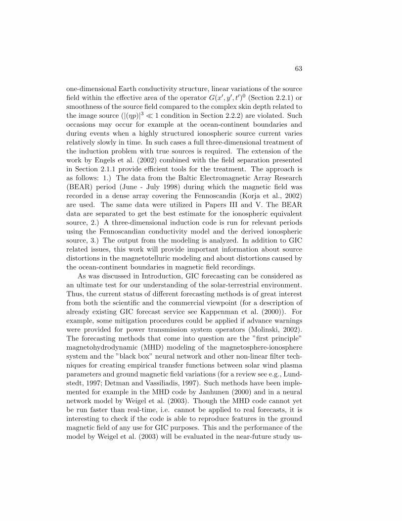
63
one-dimensional Earth conductivity structure, linear variations of the sourcefield within the effective area of the operator G(x′, y′, t′)0 (Section 2.2.1) orsmoothness of the source field compared to the complex skin depth related tothe image source (|(ηp)|3 � 1 condition in Section 2.2.2) are violated. Suchoccasions may occur for example at the ocean-continent boundaries andduring events when a highly structured ionospheric source current variesrelatively slowly in time. In such cases a full three-dimensional treatment ofthe induction problem with true sources is required. The extension of thework by Engels et al. (2002) combined with the field separation presentedin Section 2.1.1 provide efficient tools for the treatment. The approach isas follows: 1.) The data from the Baltic Electromagnetic Array Research(BEAR) period (June - July 1998) during which the magnetic field wasrecorded in a dense array covering the Fennoscandia (Korja et al., 2002)are used. The same data were utilized in Papers III and V. The BEARdata are separated to get the best estimate for the ionospheric equivalentsource, 2.) A three-dimensional induction code is run for relevant periodsusing the Fennoscandian conductivity model and the derived ionosphericsource, 3.) The output from the modeling is analyzed. In addition to GICrelated issues, this work will provide important information about sourcedistortions in the magnetotelluric modeling and about distortions caused bythe ocean-continent boundaries in magnetic field recordings.
As was discussed in Introduction, GIC forecasting can be considered asan ultimate test for our understanding of the solar-terrestrial environment.Thus, the current status of different forecasting methods is of great interestfrom both the scientific and the commercial viewpoint (for a description ofalready existing GIC forecast service see Kappenman et al. (2000)). Forexample, some mitigation procedures could be applied if advance warningswere provided for power transmission system operators (Molinski, 2002).The forecasting methods that come into question are the ”first principle”magnetohydrodynamic (MHD) modeling of the magnetosphere-ionospheresystem and the ”black box” neural network and other non-linear filter tech-niques for creating empirical transfer functions between solar wind plasmaparameters and ground magnetic field variations (for a review see e.g., Lund-stedt, 1997; Detman and Vassiliadis, 1997). Such methods have been imple-mented for example in the MHD code by Janhunen (2000) and in a neuralnetwork model by Weigel et al. (2003). Though the MHD code cannot yetbe run faster than real-time, i.e. cannot be applied to real forecasts, it isinteresting to check if the code is able to reproduce features in the groundmagnetic field of any use for GIC purposes. This and the performance of themodel by Weigel et al. (2003) will be evaluated in the near-future study us-

64 CHAPTER 4. DISCUSSION
ing the data and experience from the April 2000 event that was discussed inSection 3.2. It should be noted that it is not realistic to anticipate one-to-onecorrespondence between observed and modeled GIC but rather indicationsof regions where GIC activity may be expected.
To draw more quantitative conclusions about the relative importance ofdifferent ionospheric drivers of large GIC discussed in Section 3.2, a rigorousclassification of a large number of GIC-related current systems is required.For large datasets, and because of the need for objectivity and the time usedin the analysis, this calls for automatized procedures in practice. Interest-ingly, there is some experience on the identification of auroral forms usingpattern recognition techniques (Syrjasuo, 2001). In principle, the problem ofidentifying ionospheric current structures, for example in terms of derivedscaling factors of elementary systems (discussed in Section 2.1), is ratherclose to the identification of auroral images. Thus, it would be very in-teresting to try to transform the ideas of pattern recognition also to theionospheric current detection and classification. This type of work wouldnaturally benefit solar-terrestrial physics in general.
It is quite clear that only the very largest GIC, like those experiencedduring the March 1989 event, are capable of producing such large effects thatcatastrophic failures of systems on the ground are possible. So, it is of greatinterest not only to estimate by using the existing data how often these typesof extreme events have occurred but also to try to extrapolate these data toconclude how intense events are possible to occur. As indicated by Langloiset al. (1996), there probably exists some constraints in the dynamics of themagnetosphere-ionosphere system that also give limit to the largest possiblegeoelectric fields and GIC. One constraint is set by the characteristics ofthe storm driver, i.e. the most extreme solar ejecta (see e.g., Tsurutani,2001). Other natural constraints could be related, for example, to the largestpossible energies released in substorms and to the shortest possible timescales associated with the release. Fig. 4.1 shows the statistical occurrenceof the total horizontal geoelectric field |E| at the Nurmijarvi GeophysicalObservatory during years 1993-2001. The geoelectric field was computedusing Relations (2.66)-(2.67) with a ground conductivity σ = 3.1 · 10−2 S/mestimated in Paper II. It can be seen that the occurrence of large geoelectricfields follows a power-law pattern, characteristic for systems exhibiting selforganized criticality (e.g., Klimas et al., 2000). If data for a long enoughperiod would exist, the constraint mechanism would cause a possibly abruptdrop in the curve. Such a drop is not evident in the statistics of Fig. 4.1, andit would be interesting to speculate how far down up the higher geoelectricfield values the power law holds.
65
10-2 10-1 100100
102
104
106
Magnitude of the electric field [V/km]
Num
ber o
f 10
s va
lues
Figure 4.1: Occurrence of the computed total horizontal geoelectric field |E|at Nurmijarvi Geophysical Observatory during years 1993-2001.

66 CHAPTER 4. DISCUSSION
Bibliography
Akasofu, S.-I., and R.P. Merrit, Electric currents in power transmission lineinduced by auroral activity, Nature, 279, 308, 1979.
Albertson, V., and J. Van Baelen, Electric and magnetic fields at the Earth’ssurface due to auroral currents, IEEE T. Power Ap. Syst., 89, 578, 1970.
Amm, O., Improved electrodynamic modeling of an omega band and analysisof its current system, J. Geophys. Res., 101, 2677, 1996.
Amm, O., Ionospheric elementary current systems in spherical coordinatesand their application, J. Geomagn. Geoelectr., 49, 947, 1997.
Amm, O., and A. Viljanen, Ionospheric disturbance magnetic field contin-uation from the ground to ionosphere using spherical elementary currentsystems, Earth, Planets and Space, 51, 431, 1999.
Amm, O., The elementary current method for calculating ionospheric cur-rent systems from multisatellite and ground magnetometer data, J. Geo-phys. Res., 106, 24843, 2001.
Anderson, C.W., L.J. Lanzerotti, and C.G. Maclennan, Outage of the L-4System and the Geomagnetic Disturbances on August 4, 1972, Bell Syst.Tech. J., 53, 1817, 1974.
Anderson, C.W., Magnetic storms and cable communications, Solar SystemPlasma Physics, ed. Kennel, C.F., Lanzerotti, L.J., and Parker, E.N.,North-Holland, Amsterdam, 1978.
Araki, T., A physical model of the geomagnetic sudden commencement, So-lar Wind Sources of Magnetospheric Ultra-Low-Frequency Waves, Geo-phys. Monogr. Ser., 81, edited by M.J. Engebretson, K. Takahashi, andM. Scholer, 183 p., AGU, Washington, D.C., 1994.
67

68 BIBLIOGRAPHY
Arfken, G., and H. Weber, Mathematical methods for physicists, AcademicPress, 4th Ed., 1995.
Barlow, W.H., On the Spontaneous Electrical Currents Observed in Wiresof the Electrical Telegraph, Phil. Trans. Roy. Soc., London, 139, 61, 1849.
Barnes, P.R., and J.W. Van Dyke, Economic Consequences of GeomagneticStorms (a summary), IEEE Power Engineering Review, November, 1990.
Berdichevsky, M., and M. Zhdanov, Advanced theory of deep geomagneticsounding, Elsevier Science Publishers B.V., Netherlands, 408 pp., 1984.
Bolduc, L., P. Langlois, D. Boteler, and R. Pirjola, A Study of Geoelectro-magnetic Disturbances in Quebec, 1. General Results, IEEE Trans. PowerDelivery, 13, 1251, 1998.
Bolduc, L., P. Langlois, D. Boteler, and R. Pirjola, A Study of Geoelectro-magnetic Disturbances in Quebec, 2. Detailed Analysis of a Large Event,IEEE Trans. Power Delivery, 15, 272, 2000.
Bolduc, L., GIC observations and studies in the Hydro-Quebec power sys-tem, J. Atmos. Sol.-Terr. Phys., 64, 1793, 2002.
Boteler, D., and M.J. Cookson, Telluric currents and their effects onpipelines in the Cook Strait region of New Zealand, Materials Perfor-mance, 27, March, 1986.
Boteler, D.H., and R.J. Pirjola, The complex-image method for calculatingthe magnetic and electric fields produced at the surface of the Earth bythe auroral electrojet, Geophys. J. Int., 132, 1, 31, 1998.
Boteler, D.H., R.J. Pirjola, and H. Nevanlinna, The Effects of GeomagneticDisturbances on Electrical Systems at the Earth’s Surface, Adv. SpaceRes., 22, 17, 1998.
Boteler, D., Geomagnetic effects on the Pipe-to-Soil Potentials of a Conti-nental Pipeline, Adv. Space Res., 26, 15, 2000.
Boteler, D., Geomagnetic hazards, Synthesis of Geological Hazards inCanada, ed. G.R, Brooks, Geological Survey of Canada, Bulletin 548,183, 2001a.
Boteler, D., Space Weather Effects on Power Systems, Space Weather, AGUGeophysical Monograph 125, 347, 2001b.
69
Brasse, H., and A. Junge, The Influene of Geomagnetic Variations onPipelines and an Application for Large-Scale Magnetotelluric DepthSounding, J. Geophys., 55, 31, 1984.
Cagniard, L., Basic theory of the magneto-telluric method of geophysicalprospecting, Geophysics, 18, 605, 1953.
Campbell, W.H., Induction of Auroral Zone Electric Currents Within theAlaska Pipeline, Pure Appl. Geophys., 116, 1143, 1978.
Carlowicz, M.J., and R.E. Lopez, Stroms from the Sun, the emerging scienceof space weather, The Joseph Henry Press, Washington, D.C., 2002.
Carrington, R.C., Description of a singular appearance seen in the Sun onSeptember 1, 1859, Monthly Notices of the Royal Astronomical Society,20, p. 13, 1860.
Chapman, S., and J. Bartels, Geomagnetism, Vol. 2, Clarendon Press, Ox-ford, 1049 pp., 1940.
Chisham, G., and D. Orr, A statistical study of the local time asymmetryof Pc 5 ULF wave characteristics observed at midlatitudes by SAMNET,J. Geophys. Res., 102, 24339, 1997.
Czech, P., S. Chano, H. Huynh, and A. Dutil, The Hydro-Qubec SystemBlackout of 13 March 1989: System Response to Geomagnetic Distur-bance, EPRI Report, TR-100450, Proceedings of Geomagnetically InducedCurrents Conference, Millbrae, California, USA, November 8-10, 1989,1992.
Daly, E.J., and A. Hilgers, Space Weather: European Space Agency Per-spectives, Space Weather, AGU Geophysical Monograph 125, 53, 2001.
Davidson, W.H., The magnetic storm of March 24, 1940 - effects in thepower system, Edison Electric Institute Bulletin, July 1940, 365, 1940.
Detman, T., and D. Vassiliadis, Review of techniques for magnetic stormforecasting, Magnetic Storms, AGU Geophysical Monograph 98, 253,1997.
Dmitriev, V., and M. Berdichevsky, The fundamental model of magnetotel-luric sounding, IEEE Proc., 67, 1034, 1979.
70 BIBLIOGRAPHY
Engels, M., T. Korja, and BEAR Working Group, Multisheet modelling ofthe electrical conductivity structure in the Fennoscandian Shield, EarthPlanets Space, 54, 559, 2002
Ferris, C., Linear Network Theory, Charles E. Merril Books, Inc., Columbus,Ohio, 1962.
Feynman, J., On space weather consequences and predictions, J. Geophys.Res., 105, 10543, 2000.
Frischknecht, F.C., Electromagnetic Physical Scale Modeling, Electromag-netic Methods in Applied Geophysics, 1, Ed. M.N. Nabighian, 365, 1988.
Fukushima, N., Generalized theorem of no ground magnetic effect of verticalcurrents connected with the Pedersen currents in the uniform-conductingionosphere, Rep. Ionos. Space Res. Jpn., 30, 35, 1976.
Gradshteyn, I.S., and I.M. Ryzhik, Table of integrals series and products,Academic Press, 1965.
Gummow, R.A., GIC effects on pipeline corrosion and corrosion controlsystems, J. Atmos. Sol.-Terr. Phys., 64, 1755, 2002.
Haines, G.V., Spherical cap harmonic analysis, J. Geophys. Res., 90, 2583,1985.
Harang, L., Maximalwerte der Erdstrom in der Nahe der Nordlichtzonewahrend sehr intesiver erdmagnetischer Storungen, Gerl., Beitr. Geo-phys., 57, 310, 1941.
Henriksen, J.F., R. Elvik, and L. Gransen, Telluric Current Corrosion onBuried Pipelines, Proceedings of the 8th Scandinavian Corrosion Congress,NKM 8, 167, 1978.
Huttunen, K.E.J., H.E.J Koskinen, T.I. Pulkkinen, A. Pulkkinen, M. Palm-roth, April 2000 storm: Solar wind driver and magnetospheric response,J. Geophys. Res., 107, doi: 10.1029/2002JA0099154, 2002.
Hakkinen, L., T.I. Pulkkinen, H. Nevanlinna, R. Pirjola, and E. Tanskanen,Effects of induced currents on Dst and on magnetic variations at mid-latitude stations, J. Geophys. Res., 107, SMP 7-1 - SMP 7-8, 2002.
71
Janhunen P., GUMICS-3 - A Global Ionosphere-Magnetosphere Couplingsimulation with High Ionospheric Resolution, ESA symposiumm Proceed-ings on Enviroment Modelling for Space-based Applications, ESTEC, No-ordwijk, NL, 233, September 2000.
Jansen, F., R. Pirjola, and R. Favre, Space weather: Hazard to Earth?,Swiss Re Publishing, 2000.
Jordan, E.C., Electromagnetic Waves and Radiating Systems, New York,Prentice-Hall, Inc., 1950.
Kallio, E., T.I. Pulkkinen, H.E.J. Koskinen, and A. Viljanen, Loading-unloading processes in the nightside ionosphere, J. Geophys. Res., 27,1627, 2000.
Kamide, Y., and W. Baumjohann, Magnetosphere-ionosphere coupling,Physics and Chemistry in Space, 23, 178 p., 1993.
Kamide, Y., Geomagnetic Storms as a Dominant Component of SpaceWeather: Classic Picture and Recent Issues, Space Storms and SpaceWeather Hazards, Nato Science Series, Kluwer Academic Publishers, 43,2001.
Kappenman, J.G., and V.D. Albertson, Bracing for Geomagnetic Storms,IEEE Spectrum, March 1990, 27, 1990.
Kappenman, J.G., Geomagnetic Storms and Their Impact on Power Sys-tems, IEEE Power Eng. Rev., May 1996, 5, 1996.
Kappenman, J.G, W.A. Radasky, J.L. Gilbert, and I.A. Erinmez, Advancedgeomagnetic storm forecasting: a risk management tool for electric powersystem operations, IEEE T. Plasma Sci., 28, 2114, 2000.
Keller, G., and F. Frischknecht, Electrical Methods n Geophysical Prospect-ing, Pergamon Press, 1970.
Kisabeth, J., and G. Rostoker, Modelling of three-dimensional current sys-tems associated with magnetospheric substorms, Geophys. J. R. astr.Soc., 49, 655, 1977.
Klimas, A.J., J.A. Valdivia, D. Vassiliadis, D.N. Baker, M. Hesse, and J.Takalo, Self-organized criticality in the substorm phenomenon and itsrelation to localized reconnection in the magnetospheric plasma sheet,J. Geophys. Res., 105, 18765, 2000.

72 BIBLIOGRAPHY
Koen, J., Geomagnetically induced currents in the Southern African elec-tricity transmission network, PhD thesis, University of Cape Town, 2002.
Korja, T., M. Engels, A.A. Zhamaletdinov, A.A. Kovtun, N.A. Palshin,M.Yu. Smirnov, A. Tokarev, V.E. Asming, L.L. Vanyan, I.L. Vardaniants,and the BEAR Working Group, Crustal conductivity in Fennoscandia -a compilation of a database on crustal conductance in the FennoscandianShield, Earth, Planets and Space, 54, 535, 2002.
Koskinen, H., E. Tanskanen, R. Pirjola, A. Pulkkinen, C. Dyer, D. Rodgers,P. Cannon, J.-C. Mandeville, and D. Boscher, Space weather effects cat-alogue, Finnish Meteorological Institute, Reports, 2001:2, 2001.
Lahiri, B.N, and A.T. Price, Electromagnetic induction in non-uniform con-ductors and and the determination of the conductivity of the earth fromterrestrial magnetic variations, Phil. Trans. Roy. Soc. Lond., A237, 509,1938.
Lam, H., D. Boteler, and L. Trichtchenko, Case studies of space weatherevents from their launching on the Sun to their impacts on power systemson the Earth, Ann. Geophys., 20, 1073, 2002.
Langlois, P., L. Bolduc, and M.C. Chouteau, Probability of Occurrence ofGeomagnetic Storms Based on a Study of the Distribution of the Electricfield Amplitudes Measured in Abitibi, Quebec, in 1993-94, J. Geomagn.Geoelectr., 48, 1033, 1996.
Lanzerotti, L.J., and G.P: Gregori, Telluric Currents: The Natural Envi-ronment and Interactions with Man-made Systems, The Earth’s ElectricalEnvironment, Nat. Acad. Press, Washington, DC, 232, 1986.
Lanzerotti, L.J., Space Weather Effects on Technologies, Space Weather,AGU Geophysical Monograph 125, 11, 2001.
Lanzerotti, L., D. Thomson, and C. Maclennan, Engineering Issues in SpaceWeather, Modern Radio Science 1999, Published for the InternationalUnion of Radio Science by Oxford University Press, 1999.
Lehtinen, M., and R. Pirjola, Currents produced in earthed conductor net-works by geomagnetically-induced electric fields, Ann. Geophys., 3, 4, 479,1985.
Loomis, E., The Great Auroral Exhibition of August 28th to September 4th,1859, American Journal of Sciences and Arts, 78, 1859.
73
Lundstedt, H., AI techniques in geomagnetic storm forecasting, MagneticStorms, AGU Geophysical Monograph 98, 243, 1997.
Mareschal, M., Modelling of natural sources of magnetospheric origin in theinterpretation of regional induction studies: a review, Surveys in Geo-physics, 8, 261, 1986.
Martin, B.A., Telluric Effects on a Buried Pipeline, Corrosion, 49, 343,1993.
McNish, A., Magnetic storms, Edison Elec. Inst. Bull., 361, July 1940.
Medford, L.V., L.J. Lanzerotti, J.S. Krauss, and C.G. Maclennan, Trans-Atlantic earth potential variations during the March 1989 magneticstorms, Geophys. Res. Lett., 16, 1145, 1989.
Mersmann, U., W. Baumjohann, F. Kuppers, and K. Lange, Analysis ofan eastward electrojet by means of upward continuation of ground-basedmagnetometer data, J. Geophys., 45, 281, 1979.
Molinski, T., Why utilities respect geomagnetically induced currents, J.Atmos. Sol-Terr. Phy., 64, 1765, 2002.
Makinen, T., Geomagnetically Induced Currents in the Finnish Power Sys-tem, Geophysical Publications, No. 32, Finnish Meteorological Institute,101 p., 1993.
Ogunade, S.O., Induced Electromagnetic Field in Oil Pipelines Under Elec-trojet Current Sources, Physics of the Earth and Planetary Interiors, 43,307, 1986.
Pang, K., and K. Yau, Ancient Observations Link Changes in Sun’s Bright-ness and Earth’s Climate, EOS Transactions, 83, 481, October 2002.
Pirjola, R., Electromagnetic induction in the Earth by a plane wave or byfields of line currents harmonic in time and space, Geophysica, 18, 1, 1982.
Pirjola, R., and M. Lehtinen, Currents Produced in the Finnish 400 kVPower Transmission Grid and in the Finnish Natural Gas Pipeline byGeomagnetically-Induced Electric Fields, Ann. Geophys., 3, 4, 485, 1985.
Pirjola, R., and A. Viljanen, Complex image method for calculating electricand magnetic fields produced by an auroral electrojet of finite length,Ann. Geophys., 16, 1434, 1998.

74 BIBLIOGRAPHY
Pirjola, R., Geomagnetic effects on Ground-Based Technological Systems,Review of Radio Science, URSI, 473, 2002.
Prescott, G.B., History, Theory and Practice of the Electric Telegraph, 4thed., Ticknor and Fields, Boston, Massachussetts, 1866.
Press, W.H., S.A. Teukolsky, W.T. Vetterling, and B.P. Flannery, Numericalrecipes in FORTRAN: the art of scientific computing, 2nd ed., CambridgeUniversity Press, Cambridge, 1992.
Pulkkinen A., A. Viljanen, R. Pirjola and BEAR Working Group, LargeGeomagnetically Induced Currents in the Finnish High-Voltage PowerSystem, Finnish Meteorological Institute, Reports, 2000:2, 2000.
Pulkkinen, A., R. Pirjola, D. Boteler, A. Viljanen, and I. Yegorov, Modellingof space weather effects on pipelines, J. Appl. Geophys., 48, 233, 2001a.
Pulkkinen, A., A. Viljanen, K. Pajunpaa, and R. Pirjola, Recordings andoccurrence of geomagnetically induced currents in the Finnish natural gaspipeline network, J. Appl. Geophys., 48, 219, 2001b.
Pulkkinen, A., O. Amm, A. Viljanen, and BEAR Working Group, Iono-spheric equivalent current distributions determined with the methodof spherical elementary current systems, J. Geophys. Res., 108, doi:10.1029/2001JA005085, 2003a.
Pulkkinen, A., A. Thomson, E. Clarke, and A. McKay, April 2000 geomag-netic storm: ionospheric drivers of large geomagnetically induced currents,Annales Geophysicae, 21, 709, 2003b.
Pulkkinen, A., O. Amm, A. Viljanen, and BEAR Working Group, Sep-aration of the geomagnetic variation field on the ground into externaland internal parts using the spherical elementary current system method,Earth, Planets and Space, 55, 117, 2003c.
Robinson, R.M, and R.A. Behnke, The U.S. National Space Weather Pro-gram: A Retrospective, Space Weather, AGU Geophysical Monograph125, 1, 2001.
Root, H.G., Earth-Current Effects on Communication-Cable Power Subsys-tems, IEEE Trans. Electr. Comp., Vol. EMC-21, 1979.
Rostoker, G., Phenomenology and physics of magnetospheric substorms, J.Geophys. Res., 101, 12955, 1996.
75
Schuster, A., The diurnal variation of terrestrial magnetism, Phil. Trans.Roy. Soc. Lond., A180, 467, 1889.
Siebert, M, and W. Kertz, Zur Zerlegung eines lokalen erdmagnetischenFeldes in ausseren und inneren Anteil, Nachr. Akad. Wiss. Gottingen,Math. - Phys. Kl. Act. IIa: 87 - 112, 1957.
Smith, A., Coupling of External Electromagnetic Fields to TransmissionLines, 2nd ed., Umi Research Pr., 1987.
Syrjasuo, M., Auroral monitoring network: From all-sky camera system toautomated image analysis, D.Sc. thesis, Finnish Meteorological Institute,Contributions, 32, 2001.
Tanskanen, E.I., A. Viljanen, T.I. Pulkkinen, R. Pirjola, L. Hakkinen, A.Pulkkinen, and O. Amm, At substorm onset, 40% of AL comes fromunderground, J. Geophys. Res., 106, 13119, 2001.
Tanskanen, E., Terrestrial substorms as a part of global energy flow, PhDthesis, Finnish Meteorological Institute, Contributions, 36, 2002.
Thomson, D.J., and J.T. Weaver, The complex image approximation forinduction in a multilayered Earth, J. Geophys. Res., 80, 123, 1975.
Trichtchenko, L., and D. Boteler, Specification of geomagnetically inducedelectric field and currents in pipeline, J. Geophys. Res., 106, 21039, 2001.
Tsurutani, B., and W. Gonzalez, The interplanetary causes of magneticstorms: A review, Magnetic Storms, AGU Geophysical Monograph 98,77, 1997.
Tsurutani, B., The interplanetary causes of magnetic storms, substormsand geomagnetic quiet, Space Storms and Space Weather Hazards, NatoScience Series, Kluwer Academic Publishers, 103, 2001.
Untiedt, J., and W. Baumjohann, Studies of polar current systems using theIMS Scandinavian magnetometer array, Space Sci. Rev., 63, 245, 1993.
Viljanen, A., and R. Pirjola, Statistics on Geomagnetically-induced Currentsin the Finnish 400 kV Power System Based on Recordings of GeomagneticVariations, J. Geomag. Geoelectr., 41, 411, 1989.
Viljanen, A., K. Kauristie, and K. Pajunpaa, On induction effects at EIS-CAT and IMAGE magnetometer stations, Geophys. J. Int., 121, 893,1995.
76 BIBLIOGRAPHY
Viljanen, A., The relation between geomagnetic variations and their timederivatives and implications for estimation of induction risk, J. Geophys.res., 24, 631, 1997.
Viljanen, A., Relation of geomagnetically induced currents and local geo-magnetic variations, IEEE Trans. Pow. Del., 13, 1285, 1998.
Viljanen, A., O. Amm, and R. Pirjola, Modeling geomagnetically inducedcurrents during different ionospheric situations, J. Geophys. Res., 104,28059, 1999.
Viljanen, A., H. Nevanlinna, K. Pajunpaa, and A. Pulkkinen, Time deriva-tive of the horizontal geomagnetic field as an activity indicator, Ann.Geophys., 19, 1107, 2001.
Viljanen, A., A. Pulkkinen, O. Amm, R. Pirjola, T. Korja, and BEAR Work-ing Group, Fast computation of the geoelectric field using the method ofelementary current system, Submitted to Ann. Geophys., 2003.
Wait, J., and K. Spies, On the image representation of the quasi-static fieldsof a line current source above the ground, Canadian Journal of Physics,47, 2731, 1969.
Wallerius, A., Solen Gav Sverige en Stromstot, (written in Swedish) Nyteknik Teknisk tidskrift, 29, 3, 1982.
Weaver, J.T., On the separation of Local Geomagnetic Fields into Externaland Internal Parts, Zeitschrift fur Geophysik, 30, 29, 1964.
Weaver, J.T., Mathematical Methods for Geo-electromagnetic Induction,Applied and engineering mathematics series, Research Studies Press Ltd.,1994.
Weigel, R.S., A.J. Klimas, and D. Vassiliadis, Solar-wind coupling and pre-dictability of ground magnetic fields and their time derivatives, in press,J. Geophys. Res., 2003.
Withbroe, G.L., Living With a Star, Space Weather, AGU GeophysicalMonograph 125, 45, 2001.

Index
aa* index, 14
adjustment distance, 45admittance, 45analogue modeling, 7aurora, 4
detection, 64auroral zone, 8, 54, 56
causality, 31complex image method, 16, 35, 40complex skin depth, 37complex square root, 29conductivity, vii, 15, 25, 27, 35
effective, 32, 35convection, 55coronal hole, 6, 7coronal mass ejection, 6, 7corrosion, 12curl-free condition, 17current wedge, 55cusp, 57
diffusion equation, 27direct-current, 39displacement current, 27distributed source transmission line
theory, 45divergence-free condition, 17, 20,
27
Earthhomogeneous, 35, 40
layered, 27, 29, 35, 38electrojet, 50, 55elementary current system method,
16, 38ESA, i, 5European Union, 6extreme events, 64
field-aligned currents, 6, 18, 20Fourier method, 25Fourier transformation, 28, 35, 38
Gauss-Schmidt method, 25geoelectric field
modeling, 28, 35properties, 26, 49
geomagnetic storm, see magneticstorm
geomagnetically induced currents,10
economic impact, 10effects
communication cables, 11pipelines, 12power systems, 10railways, 12telegraph, 4, 6, 10
forecast, 63modeling
continuously grounded sys-tems, 45
discretely grounded systems,39
77

78 INDEX
reported occasions, 14Green’s function, 18
half-cycle saturation, 10
impedance, 29, 30, 35, 36, 40, 45ionospheric currents, see ionospheric
equivalent currentsionospheric equivalent currents
classification, 64derivation, 16properties, 54
K index, 52Kirchhoff’s law, 43
least squares, 22, 26linearly varying field, 33
magnetic field separation, 23, 24,63
magnetic pulsations, 56magnetic storm, 6, 8, 56magnetohydrodynamic modeling, 63magnetosphere, 3, 8, 56magnetotelluric method, 34, 63Maxwell’s equations, 26
neural networks, 63NOAA, 5
Ohm’s law, 26omega band, 56
pattern recognition, 64permeability, vii, 26permittivity, viiplane wave method, 34, 52power law, 64
quasi-static field, 27, 31
reconnection, 8
scaling factor, 21, 22, 25, 39sea-continent boundary, 63self organized criticality, 57, 64singular value decomposition, 22,
26skin depth, 51solar wind, 3, 7space environment center, 5space weather
definition, 4economic impact, ieffects, 4physics, 7
spatial method, 25spectral impedance, see impedancespherical cap harmonic analysis, 16,
25spherical elementary current sys-
tem method, see elemen-tary current system method
spherical harmonic method, 16substorm, 8, 55, 56, 64sudden commencement, 56Sun, 3, 7
Thevenin theorem, 46time derivative of the magnetic field,
35, 50
US Air Force, 5