Embed Size (px)
Citation preview
| i
FIRE SAFETY AND SUPPRESSION IN
MODERN RESIDENTIAL BUILDINGS |
Research on the Influence of the Building Skin on the Fire
Behaviour in Well Insulated and Airtight Dwellings and
Consequences for the Safety of the Occupant and Fire
Service
THESIS
BUILDING
TECHNOLOGY
| iii
THESIS
BUILDING
TECHNOLOGY
This thesis is submitted in order to acquire the title MSc for
the master track Building Technology, of the Department
Architecture, Building and Planning at the Eindhoven
University of Technology
- Department Architecture, Building and Planning -
Building Technology
Student V. van den Brink
078 3686
Supervisors
Prof. dr. ir. H.J.H. Brouwers (Chairman)
Ir. R.A.P. van Herpen FIFireE (Fellow TU/e)
Dr. ir. R. Weewer (Instituut Fysieke Veiligheid - Brandweeracademie)
Ir. A.C.J. de Korte (Supervisor TU/e)
Date: 21-04-2015

iv |

| v
Preface
In the context of the study Building Technology, which is a part of the department Architecture,
Building and Planning of the Eindhoven University of Technology, I conducted this research which
focuses on the fire behaviour and the occurrence of pressure build-up in well insulated and airtight
dwellings. This research is conducted in response to the problem statement which has been provided
by Brandweer Nederland. During their daily activities the trend is observed that window panes
withstand the fire longer before they lose its structural integrity. Because this has major implications
for the fire scenario and safety of fire fighters during the suppressive phase, the question was initially
aimed to provide an insight in the pane behaviour of modern dwellings.
In a recently conducted research of Ronald Huizinga, a thorough study to the performance of double
and triple glazing on the fire behaviour was already carried out. In his thesis, the fall out period of
double and triple glazing was identified. Another study presented on the National Congress Fire
Safety Engineering in 2013 by Brecht Debrouwere, was a research to the fire behaviour in low energy
houses. It was found that the fire behaviour in this kind of dwellings is more extreme compared to
conventional dwellings. One interesting conclusion was that the inner pressure in low energy houses
might reach values in the order of hundreds of Pascal. From the perspective of the fire service this
would mean that the observed trend will not continue as this magnitude of pressure will have a
certain effect on the structural integrity of window panes. The findings of these studies have in
consultation with Brandweer Nederland led to the research question as formulated in chapter two.
The first part of this report is theoretical in nature. In this part the research methodology is pointed
out and the basics of pressure during a fire will be pointed out. In the second part of the report,
simulations will be carried out to identify the fire behaviour in well insulated and airtight dwellings
and in the third part these results will be validated by conducting experiments and the results are
described.
This study has been realized in cooperation with Stichting Fellowship FSE WO2 and Brandweer
Nederland. In addition, several people have contributed to this research. I would take this
opportunity to thank the supervisors Prof. Brouwers, Ir. Van Herpen, Ir. De Korte and Dr. Weewer for
their support during the graduation process.
Moreover I want to thank the Fire Department Twente, and in particular Folkert van der
Ploeg for the pleasant cooperation, practical guidance and the possibilities that were offered to
conduct the experiments on TroNed (Trainings- en Oefencentrum brandweer Oost-Nederland). This
made it possible to investigate the pressure build-up during a fire in a well insulated dwelling on real
scale, and was therefore essential for my research. The materials for the experiments are sponsored
by Mr. Cleef of Rockwool. I want to thank for your contribution to this research. Additionally I would
like to thank Sylvia Brandenburg, Martin Harbers and Ronald Huizinga of Nieman Raadgevende
Ingenieurs for the support during the Voltra analysis as the preparation for the real scale fire
experiments and their support with the blowerdoor test. Finally I want to thank Dr. Regterschot from
the Eindhoven University of Eindhoven for the contribution to the research. His view and critical
comments has led to an improvement of the quality in general and in particular the statistical part of
the study.
Vincent van den Brink
Eindhoven, 21 April 2015
vi |
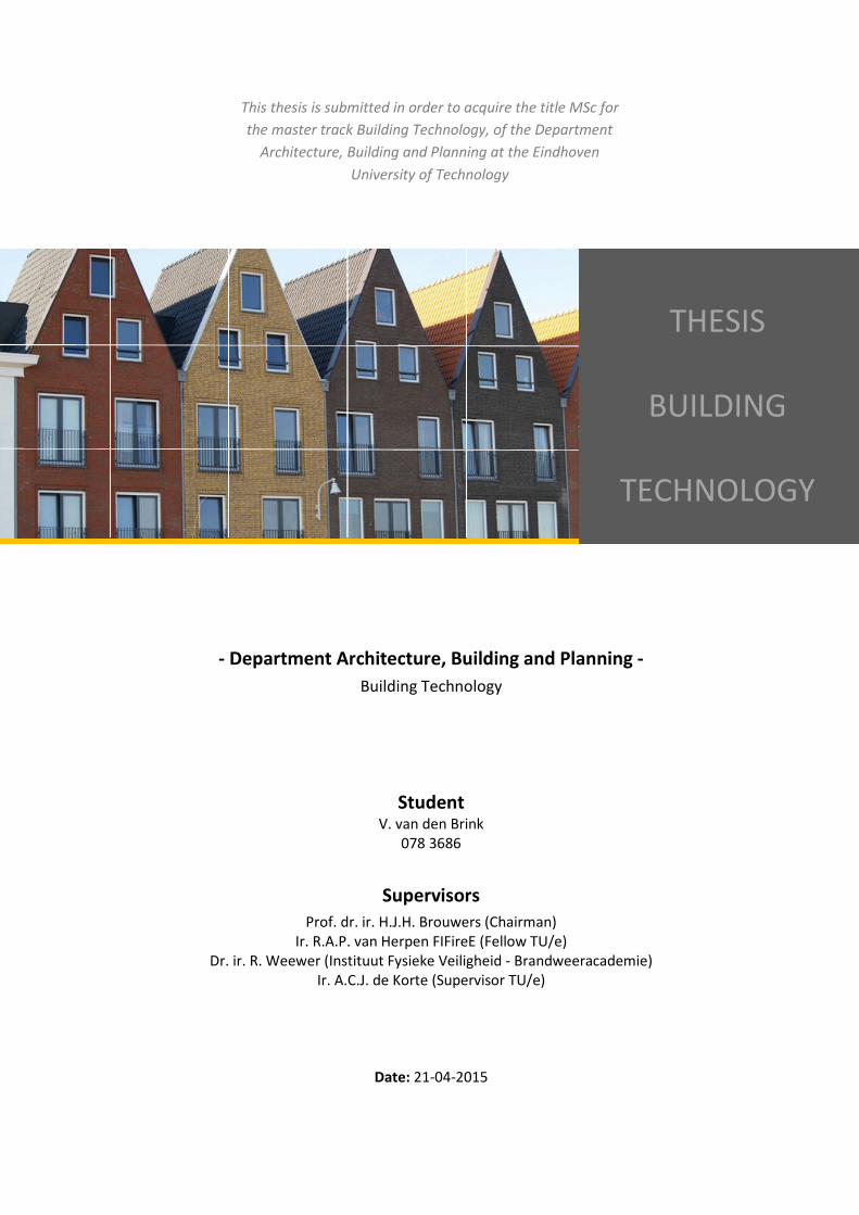
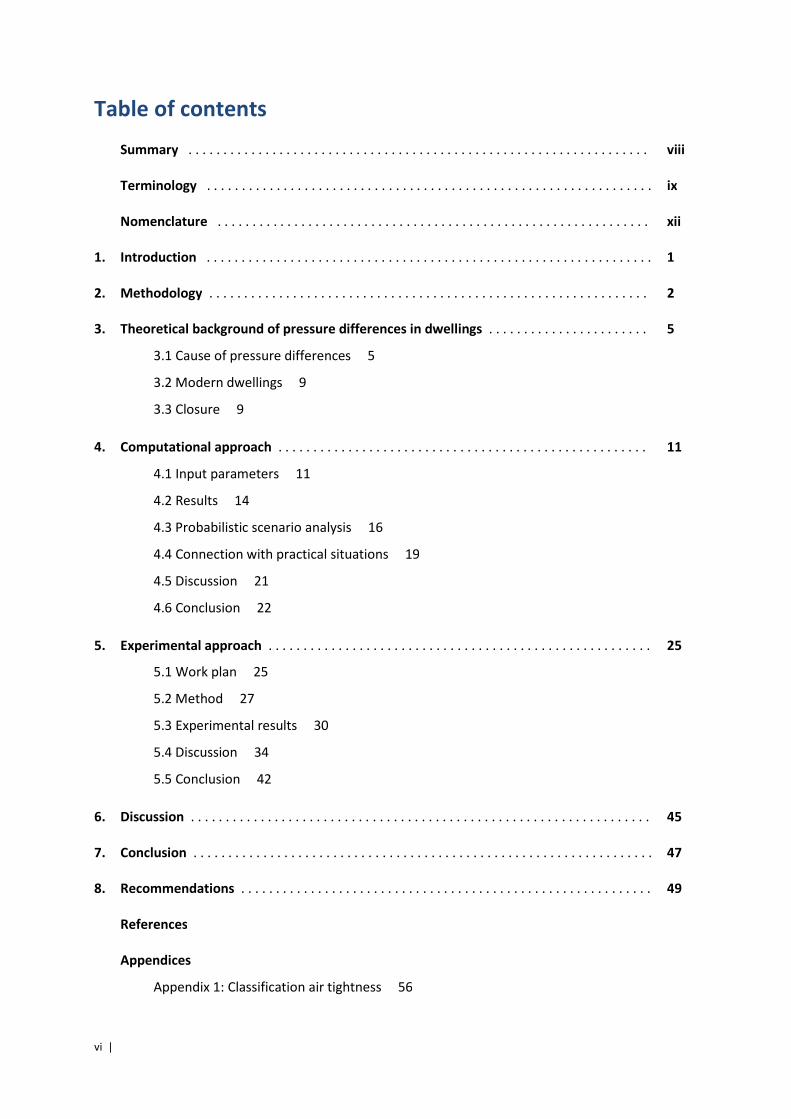
Table of contents
Summary . . . . . . . . . . . . . . . . . . . . . . . . . . . . . . . . . . . . . . . . . . . . . . . . . . . . . . . . . . . . . . . . . . viii
Terminology . . . . . . . . . . . . . . . . . . . . . . . . . . . . . . . . . . . . . . . . . . . . . . . . . . . . . . . . . . . . . . . .
ix
Nomenclature . . . . . . . . . . . . . . . . . . . . . . . . . . . . . . . . . . . . . . . . . . . . . . . . . . . . . . . . . . . . . .
xii
1. Introduction . . . . . . . . . . . . . . . . . . . . . . . . . . . . . . . . . . . . . . . . . . . . . . . . . . . . . . . . . . . . . . . .
1
2. Methodology . . . . . . . . . . . . . . . . . . . . . . . . . . . . . . . . . . . . . . . . . . . . . . . . . . . . . . . . . . . . . . . 2
3. Theoretical background of pressure differences in dwellings . . . . . . . . . . . . . . . . . . . . . . . 5
3.1 Cause of pressure differences 5
3.2 Modern dwellings 9
3.3 Closure 9
4. Computational approach . . . . . . . . . . . . . . . . . . . . . . . . . . . . . . . . . . . . . . . . . . . . . . . . . . . . . 11
4.1 Input parameters 11
4.2 Results 14
4.3 Probabilistic scenario analysis 16
4.4 Connection with practical situations 19
4.5 Discussion 21
4.6 Conclusion 22
5. Experimental approach . . . . . . . . . . . . . . . . . . . . . . . . . . . . . . . . . . . . . . . . . . . . . . . . . . . . . . . 25
5.1 Work plan 25
5.2 Method 27
5.3 Experimental results 30
5.4 Discussion 34
5.5 Conclusion 42
6. Discussion . . . . . . . . . . . . . . . . . . . . . . . . . . . . . . . . . . . . . . . . . . . . . . . . . . . . . . . . . . . . . . . . . . 45
7. Conclusion . . . . . . . . . . . . . . . . . . . . . . . . . . . . . . . . . . . . . . . . . . . . . . . . . . . . . . . . . . . . . . . . . . 47
8. Recommendations . . . . . . . . . . . . . . . . . . . . . . . . . . . . . . . . . . . . . . . . . . . . . . . . . . . . . . . . . . . 49
References
Appendices
Appendix 1: Classification air tightness 56
| vii
Appendix 2: Input Ozone Chapter 4 “Computational Approach” 57
Appendix 3: Alternative approach iterative calculation process 62
Appendix 4: Uncertainties in simulations 64
Appendix 5: Parameter study – Results 66
Appendix 6: Results probabilistic scenario analysis 72
Appendix 7: Multiple linear regression model 74
Appendix 8: Calculation insulation covering for experimental enclosure 75
Appendix 9: Results blowerdoor test 77
Appendix 10: Simulation experimental scenarios 79
Appendix 11: Fuel calculation experiments 83
Appendix 12: Analysis moment of deflection of the temperature curves on the basis
o of the slope of the line 86
Appendix 13: Overview fitted simulation models 87
Appendix 14: Mass loss rate free burning rate 88
Appendix 15: Stepwise increase RHR in 20 s. 89
Appendix 16: Temperature behaviour scenario 3 and 4 91
viii |
Summary
During their daily activities the fire service observed that there is a trend that glass fallout occurs at a
later stage of the fire. The extended period of time before the window pane fallout has major
implications for the fire behaviour, and therefore also the strategy of the fire service. As a result, it is
expected that the fire service will face more ventilated controlled fires in the near future, which
result in a faster increase of the temperature, the production of more toxic gases whereby the
survivability for the occupant decrease dramatically. The occurrence of a quick increase of the Rate
of heat Release (RHR), backdraft, smoke gas explosion or a sudden window pane failure as a result of
high pressures might result in more casualties among fire fighters. The Dutch building code will
prescribe that in the year 2020 all buildings must be energy neutral. An insight in the consequences
for the safety of the occupant and fire service is therefore essential.
In this research, a study to the influence of the building skin on the fire behaviour, and in particular
the pressure increase during fire in well insulated and airtight dwellings, is carried out. This makes it
possible to make statements about the safety of the occupant and the fire service during suppressive
actions in modern dwellings.
The literature study identified that the pressure build-up mainly depends on thermal
expansion. The thermal expansion is determined by six concrete variables which are the Rate of Heat
Release (RHR), amount of infiltration (qv;10 value), volume of the room, mechanical ventilation, type
of enclosure and the Rc- value of the enclosure. The qv;10 value, size of the compartment and the RHR
have the largest influence on the pressure behaviour.
It appeared that on the basis of the simulation programme Ozone, it is difficult to give an insight in
the fire and pressure behaviour of well insulated and airtight dwellings as a flow exponent of n ≠ 0.5
cannot be applied. The magnitude of the air flow is calculated at a fixed pressure difference of 10 Pa
and an oxygen dependent combustion model is lacking. With regard to the first two aspects an
iterative calculation tool is developed to make a closer approach for the pressure behaviour.
However, it appeared that this results in an underestimation of the pressure.
For the simulated scenario in an enclosure of 4.0 x 5.0 x 2.6 m (l x w x h), this results in a
pressure peak of 64 Pa. As a result of the stochastic deviation of the variables and a lack of
knowledge about practical situations, it can be expected that the pressure peak of 64 Pa will be
exceeded. A multiple linear regression model is used to develop an equation to predict the pressure
peak within a range of the variables of +/- 50% with regard to that scenario in practical situations.
The results of the conducted experiments show that that high pressures in the order of hundreds of
Pa can occur during fires in passive dwellings. But also for well insulated dwellings significant higher
pressures are observed. In the situation in which the amount of infiltration is doubled with regard to
the maximum amount of infiltration according the passive house standard, still a pressure peak is
173 Pa observed.
Although in theory a ventilation controlled fire can be expected in modern dwellings, in practice the
fire and pressure behaviour will be determined by coincidental factors like opened door and
windows. Therefore, the fire service can expect a wide range of scenarios. The pressure peak will
occur before arrival of the fire service at the fire scene and will therefore have no direct influence on
the safety of the fire service.
The high pressures will have an influence on the safety of the occupant as the pressure peak
will occur during the fire growth stage. This may prevent the occupant to escape the dwelling as it
will be difficult or even impossible to open inward turning doors. In combination with the strong
temperature increase this will lead to fatal circumstances within a minute.
| ix
Terminology
Adiabatic
A process is adiabatic when there is no heat exchange with the
environment.
Backdraft
A phase transition whereby a sudden supply of oxygen into an enclosure
with depleted oxygen supply leads to a rapidly and sudden combustion
of the gaseous combustion products.
CFAST A two zone mathematical model which evaluate the distribution of
smoke, fire gases en temperatures throughout compartments of a
building during fire.
Computational Fluid
dynamics (CFD)
Advanced computer models in general which describes on the basis of a
certain mesh (local) flows, velocity, temperatures and concentration of
fluids and gases. Allows solving problems which cannot be solved
analytically.
Deterministic model
Model which present its output as a single value. No variation limits are
given, and so no uncertainty is taken into account.
Equivalent surface
One single opening which corresponds to the sum of all infiltration
openings.
External validity Relationship between the scientific model and real situations; To which
extent predicts the research design real world conditions.
Fire Dynamics Simulator
(FDS)
An open source Large Eddy Simulation CFD model, which numerically
solves equations which describes low speed flows with the emphasis on
heat and smoke transport during fires.
Fire Safety Engineering
A scientific and project specific approach to create a certain level of
building safety based on the application of engineering principles.
Flashover
A rapid phase transition whereby the hot gases within the compartment
set the entire compartment on fire in a short period of time by
convection or radiation.
Fuel controlled fire
Fire scenario in which enough oxygen is present for combustion. The
existence of the fire depends on the amount of fuel present in the fire
room.
Internal validity The extent to which the reasoning in the research is carried out
correctly; Is measured what was intended to be measured.
Laboratory conditions
The extent to which the researcher can control the environmental
factors of the experiment.
Local fire Situation whereby the fire is limited to its initial object or surrounding
objects; only a part of the compartment is burning.
x |
Mass loss rate The mass released per second from a material during fire.
Model A combination of several hypotheses with regard to the distribution and
consistency between the variables.
Neutral plane
Horizontal plane in the fire room with an equal pressure as the ambient
pressure
One zone model A zone model in which the assumption of a uniform temperature in the
fire room is made.
Ozone A two zone mathematical model which evaluate the temperature
development in a single compartment during a fire.
Passive house
Building concept which emphasizes the use of little energy in order to
relieve the environment with respect to the carbon dioxide release. This
is achieved by applying small, properly orientated windows, high
Rc-values and a high degree of air-tightness.
qv;10
Volume of the air flow through the building envelope measured at a
pressure difference of 10 Pa.; A term for the degree of air-tightness of a
building.
Rate of Heat Release
(RHR)
The heat released per second from a material during fire.
Rc- value
Thermal resistance of the building envelope; The resistance of a
structure against heat transition.
Risk The multiplication of the probability that an unwanted event occurs
with the consequences.
Stoichiometry A situation in which the molar ratio is such that there is enough oxygen
for complete combustion.
Thermal thick In a thermal thick structure, accumulation takes place when the
temperature within the enclosure increases. When the temperature
within the enclosure decreases, the heat will be dissipated.
Thermal thin In a thermal thin structure no accumulation of the heat can take place.
In case of an uninsulated thermal thin structure the heat will be
dissipated to its environment.
Two zone model
A zone model in which during the simulation a hot upper layer under
the ceiling with an uniform temperature and a lower layer in which no
smoke is present with an uniform temperature are distinguished. The
layers are separated from each other by a neutral plane.
Validation
Determining the correctness of the applied model and to which extent
the made assumptions are correct.

| xi
Ventilation controlled
fire
Situation in which there is not sufficient oxygen for complete
combustion. The Rate of Heat Release is then controlled by the amount
of oxygen available in the fire room.
Verification Determining to which extent the result of the model is correct.
xii |
Nomenclature
Symbol
Description
Unit
A Area m2
Ae Equivalent surface m2
An Equivalent surface upper opening m2
Au Equivalent surface lower opening m2
c Partial air leakage coefficient dm3/s.m
1.Pa
n
cv Specific heat J/kg.K
C Total air leakage coefficient dm3/s. Pa
n
Cp Wind pressure coefficient [-]
g Gravitational constant m/s2
h Height m
hn Height above the neutral plane m
hu Height below the neutral plane m
Hc Heat of combustion [-]
k Extinction absorption coefficient [-]
l Length m
m Mass kg/m3
m” Corrected free burning rate kg/s
m∞” Free burning rate kg/s
n Flow exponent [-]
nm Number of moles [-]
N Ventilation rate [-]
p1 Fire activation probability [-]
pfi Probability of the occurrence of fire [-]
pf;fi Probability of failure [-]
pt Failure probability [-]
P Pressure Pa
Pw Wind pressure Pa
ΔPn Pressure difference in the dwelling Pa
ΔPu Atmospheric pressure Pa
q Volume flow per unit area m3/s.m
2
�� Rate of Heat Release kW
r Air flow resistance m-4
re Air flow resistance exhaust branch m-4
ri Air flow resistance inlet branch m-4
rl Air flow resistance leakages m-4
R Gas constant J/mole.K
t Time s
T Temperature K
| xiii
Symbol Description Unit
Te Temperature of the outflowing gases K
Tg Temperature inside the dwelling K
v Air current speed m/s
va Air current speed into enclosure m/s
vg Air current speed out enclosure m/s
V Compartment volume m3
w Width m
Greek symbols
ß Regression coefficient [-]
λ Thermal conductivity W/m.K
χ Combustion efficiency [-]
ɛ Error term [-]
μ Contraction coefficient (Bernoulli coefficient) [-]
ρ Density kg/m3
ρa Air density outside the dwelling kg/m3
ρg Air density inside the dwelling kg/m3

xiv |
| 1
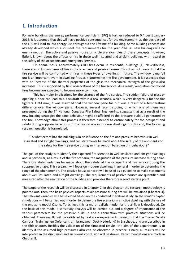
1. Introduction
For new buildings the energy performance coefficient (EPC) is further reduced to 0.4 per 1 January
2015. It is assumed that this will have positive consequences for the environment, as the decrease of
the EPC will lead to less energy use throughout the lifetime of a building. Some building concept are
already developed which also meet the requirements for the year 2020 as new buildings will be
energy neutral. The active and passive house principle are examples of these concepts. However,
little is known about the effects of fire in these well insulated and airtight buildings with regard to
the safety of the occupants and emergency services.
On annual basis, approximately 4100 fires occur in residential buildings [1]. Nevertheless,
there are no known cases of fire in these active and passive houses. This does not prevent that the
fire service will be confronted with fires in these types of dwellings in future. The window pane fall
out is an important event in dwelling fires as it determines the fire development. It is suspected that
with an increase of the thermal properties of the glass the mechanical strength of the glass also
increases. This is supported by field observations of the fire service. As a result, ventilation controlled
fires become are expected to become more common.
This has major implications for the strategy of the fire service. The sudden failure of glass or
opening a door can lead to a backdraft within a few seconds, which is very dangerous for the fire
fighters. Until now, it was assumed that the window pane fall out was a result of a temperature
difference over the window pane. However, several recent studies, of which one of them was
presented during the 6th
National Congress Fire Safety Engineering, suggests that as a result of the
new building strategies the pane behaviour might be affected by the pressure build-up generated by
the fire. Knowledge about this process is therefore essential to ensure safety for the occupant and
safety during suppressive actions of the fire service in modern dwellings. To this end, the following
research question is formulated:
“To what extent has the building skin an influence on the fire and pressure behaviour in well
insulated and airtight dwellings, and can statements be made about the safety of the occupant and
the safety for the fire service during an intervention based on this behaviour?”
The goal of the study is to identify the expected fire scenario in well insulated and airtight dwellings
and in particular, as a result of the fire scenario, the magnitude of the pressure increase during a fire.
Therefore statements can be made about the safety of the occupant and fire service during the
suppressive phase. This research will focus on modern dwellings in general in order to determine the
range of the phenomenon. The passive house concept will be used as a guideline to make statements
about well insulated and airtight dwellings. The requirements of passive houses are quantified and
measured after the realization of the building and provides therefore a good starting point.
The scope of the research will be discussed in Chapter 2. In this chapter the research methodology is
pointed out. Then, the basic physical aspects of air pressure during fire will be explained (Chapter 3).
The relevant variables will be selected based on the conducted literature study. In the fourth chapter
simulations will be carried out in order to define the fire scenario in a fictive dwelling with the use of
the one zone model Ozone. To achieve this, a more realistic model for the airflow is developed. On
the basis of this model a sensitivity analysis will be carried out and a degree of importance of the
various parameters for the pressure build-up and a connection with practical situations will be
obtained. These results will be validated by real scale experiments carried out at the Troned Safety
Campus (Trainings- en Oefencentrum brandweer Oost-Nederland) in Enschede, and are described in
the fifth chapter. Besides the validation of the simulated results, the aim of the experiments is to
identify if the assumed high pressures also can be observed in practice. Finally, all results will be
interpreted in the discussion and an overall conclusion will be drawn. Recommendations are made in
Chapter 8.
2 |
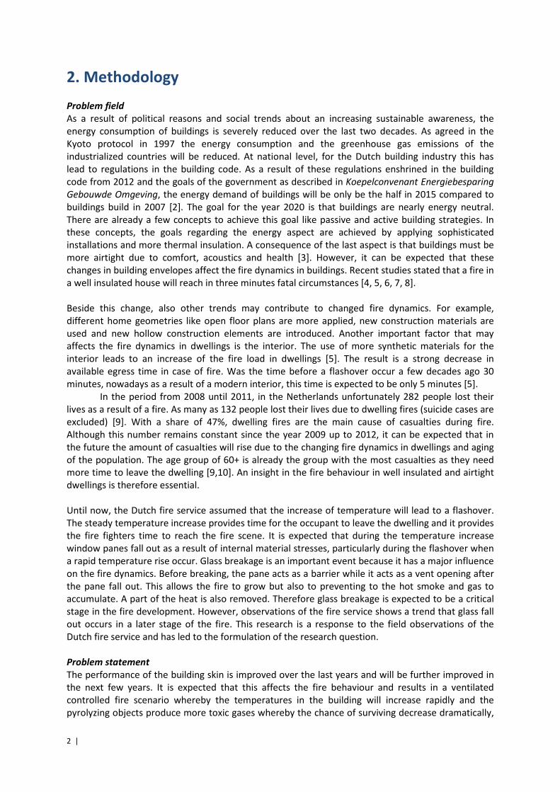
2. Methodology
Problem field
As a result of political reasons and social trends about an increasing sustainable awareness, the
energy consumption of buildings is severely reduced over the last two decades. As agreed in the
Kyoto protocol in 1997 the energy consumption and the greenhouse gas emissions of the
industrialized countries will be reduced. At national level, for the Dutch building industry this has
lead to regulations in the building code. As a result of these regulations enshrined in the building
code from 2012 and the goals of the government as described in Koepelconvenant Energiebesparing
Gebouwde Omgeving, the energy demand of buildings will be only be the half in 2015 compared to
buildings build in 2007 [2]. The goal for the year 2020 is that buildings are nearly energy neutral.
There are already a few concepts to achieve this goal like passive and active building strategies. In
these concepts, the goals regarding the energy aspect are achieved by applying sophisticated
installations and more thermal insulation. A consequence of the last aspect is that buildings must be
more airtight due to comfort, acoustics and health [3]. However, it can be expected that these
changes in building envelopes affect the fire dynamics in buildings. Recent studies stated that a fire in
a well insulated house will reach in three minutes fatal circumstances [4, 5, 6, 7, 8].
Beside this change, also other trends may contribute to changed fire dynamics. For example,
different home geometries like open floor plans are more applied, new construction materials are
used and new hollow construction elements are introduced. Another important factor that may
affects the fire dynamics in dwellings is the interior. The use of more synthetic materials for the
interior leads to an increase of the fire load in dwellings [5]. The result is a strong decrease in
available egress time in case of fire. Was the time before a flashover occur a few decades ago 30
minutes, nowadays as a result of a modern interior, this time is expected to be only 5 minutes [5].
In the period from 2008 until 2011, in the Netherlands unfortunately 282 people lost their
lives as a result of a fire. As many as 132 people lost their lives due to dwelling fires (suicide cases are
excluded) [9]. With a share of 47%, dwelling fires are the main cause of casualties during fire.
Although this number remains constant since the year 2009 up to 2012, it can be expected that in
the future the amount of casualties will rise due to the changing fire dynamics in dwellings and aging
of the population. The age group of 60+ is already the group with the most casualties as they need
more time to leave the dwelling [9,10]. An insight in the fire behaviour in well insulated and airtight
dwellings is therefore essential.
Until now, the Dutch fire service assumed that the increase of temperature will lead to a flashover.
The steady temperature increase provides time for the occupant to leave the dwelling and it provides
the fire fighters time to reach the fire scene. It is expected that during the temperature increase
window panes fall out as a result of internal material stresses, particularly during the flashover when
a rapid temperature rise occur. Glass breakage is an important event because it has a major influence
on the fire dynamics. Before breaking, the pane acts as a barrier while it acts as a vent opening after
the pane fall out. This allows the fire to grow but also to preventing to the hot smoke and gas to
accumulate. A part of the heat is also removed. Therefore glass breakage is expected to be a critical
stage in the fire development. However, observations of the fire service shows a trend that glass fall
out occurs in a later stage of the fire. This research is a response to the field observations of the
Dutch fire service and has led to the formulation of the research question.
Problem statement
The performance of the building skin is improved over the last years and will be further improved in
the next few years. It is expected that this affects the fire behaviour and results in a ventilated
controlled fire scenario whereby the temperatures in the building will increase rapidly and the
pyrolyzing objects produce more toxic gases whereby the chance of surviving decrease dramatically,
| 3
especially in dwellings. The trend is also dangerous for the fire service. A sudden supply of oxygen to
a ventilated controlled fire can result in a backdraft or smoke gas explosion and therefore cause
casualties. Therefore, the improved performance of the building skin has major implications for the
strategy of the fire service and it constitutes a risk for both the occupant and fire fighters. So
knowledge about the fire dynamics and the different variables of glass breakage is important for
strategic choices of the fire service and the safety of the occupant and fire service. Until now it was
assumed that internal material stresses as a result of thermal differences within a window pane is
the main cause for fall out. However, recent research shows that for well insulated dwellings the
increasing inner pressure may become an important factor for determining the moment of window
pane fall out. More knowledge about the fire and pressure behaviour in well insulated and airtight
dwellings is therefore required.
Research objective
The objective of the research is to contribute to the safety of the dwelling occupant and the fire
service during suppressive actions in case of fires in well insulated dwellings. The goal is to identify
the influence of the building skin on the expected fire and pressure behaviour in well insulated and
airtight dwellings by taking all possible fire scenarios into account. Recommendations for the strategy
of fire suppression will be provided.
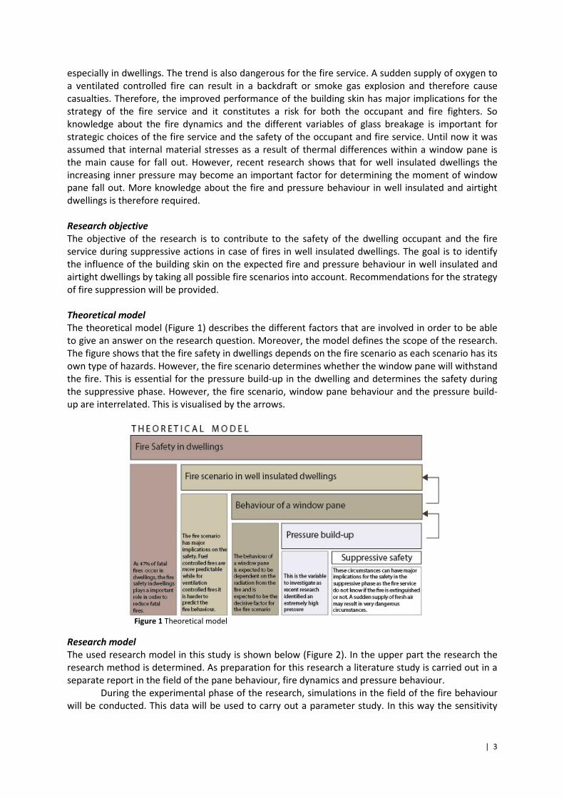
Theoretical model
The theoretical model (Figure 1) describes the different factors that are involved in order to be able
to give an answer on the research question. Moreover, the model defines the scope of the research.
The figure shows that the fire safety in dwellings depends on the fire scenario as each scenario has its
own type of hazards. However, the fire scenario determines whether the window pane will withstand
the fire. This is essential for the pressure build-up in the dwelling and determines the safety during
the suppressive phase. However, the fire scenario, window pane behaviour and the pressure build-
up are interrelated. This is visualised by the arrows.
Figure 1 Theoretical model
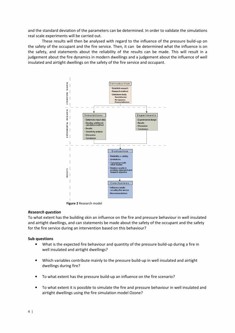
Research model
The used research model in this study is shown below (Figure 2). In the upper part the research the
research method is determined. As preparation for this research a literature study is carried out in a
separate report in the field of the pane behaviour, fire dynamics and pressure behaviour.
During the experimental phase of the research, simulations in the field of the fire behaviour
will be conducted. This data will be used to carry out a parameter study. In this way the sensitivity
4 |
and the standard deviation of the parameters can be determined. In order to validate the simulations
real scale experiments will be carried out.
These results will then be analysed with regard to the influence of the pressure build-up on
the safety of the occupant and the fire service. Then, it can be determined what the influence is on
the safety, and statements about the reliability of the results can be made. This will result in a
judgement about the fire dynamics in modern dwellings and a judgement about the influence of well
insulated and airtight dwellings on the safety of the fire service and occupant.
Figure 2 Research model
Research question
To what extent has the building skin an influence on the fire and pressure behaviour in well insulated
and airtight dwellings, and can statements be made about the safety of the occupant and the safety
for the fire service during an intervention based on this behaviour?
Sub questions
• What is the expected fire behaviour and quantity of the pressure build-up during a fire in
well insulated and airtight dwellings?
• Which variables contribute mainly to the pressure build-up in well insulated and airtight
dwellings during fire?
• To what extent has the pressure build-up an influence on the fire scenario?
• To what extent it is possible to simulate the fire and pressure behaviour in well insulated and
airtight dwellings using the fire simulation model Ozone?
| 5
3. Theoretical background of pressure differences in
dwellings
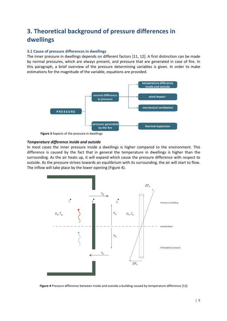
3.1 Cause of pressure differences in dwellings
The inner pressure in dwellings depends on different factors [11, 12]. A first distinction can be made
by normal pressures, which are always present, and pressure that are generated in case of fire. In
this paragraph, a brief overview of the pressure determining variables is given. In order to make
estimations for the magnitude of the variable, equations are provided.
Figure 3 Aspects of the pressure in dwellings
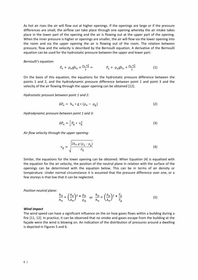
Temperature difference inside and outside
In most cases the inner pressure inside a dwellings is higher compared to the environment. This
difference is caused by the fact that in general the temperature in dwellings is higher than the
surrounding. As the air heats up, it will expand which cause the pressure difference with respect to
outside. As the pressure strives towards an equilibrium with its surrounding, the air will start to flow.
The inflow will take place by the lower opening (Figure 4).
Figure 4 Pressure difference between inside and outside a building caused by temperature difference [12]
6 |
As hot air rises the air will flow out at higher openings. If the openings are large or if the pressure
differences are small, the airflow can take place through one opening whereby the air intake takes
place in the lower part of the opening and the air is flowing out at the upper part of the opening.
When the inner pressure is higher or openings are smaller, the air will flow via the lower opening into
the room and via the upper opening the air is flowing out of the room. The relation between
pressure, flow and the velocity is described by the Bernoulli equation. A derivative of the Bernoulli
equation can be used for the hydrostatic pressure between the upper and lower part:
Bernoulli’s equation: �� + ρ�gh� + �� ��� = �� + ρ�gh� + �� ��� (1)
On the basis of this equation, the equations for the hydrostatic pressure difference between the
points 1 and 2, and the hydrodynamic pressure difference between point 1 and point 3 and the
velocity of the air flowing through the upper opening can be obtained [12].
Hydrostatic pressure between point 1 and 2:
ΔP� = h� ∗ g ∗ (ρ� −ρ�) (2)
Hydrodynamic pressure between point 1 and 3:
ΔP� = �� P� ∗ v�� (3)
Air flow velocity through the upper opening:
v� = �2ℎ!"(ρ#–ρg)ρg (4)
Similar, the equations for the lower opening can be obtained. When Equation (4) is equalised with
the equation for the air velocity, the position of the neutral plane in relation with the surface of the
openings can be determined with the equation below. This can be in terms of air density or
temperature. Under normal circumstance it is assumed that the pressure difference over one, or a
few storeys is that low that it can be neglected.
Position neutral plane:
%�%� = &'�'�(2
* )*)+ or
%�%� = &'�'�(2 *
,*,+ (5)
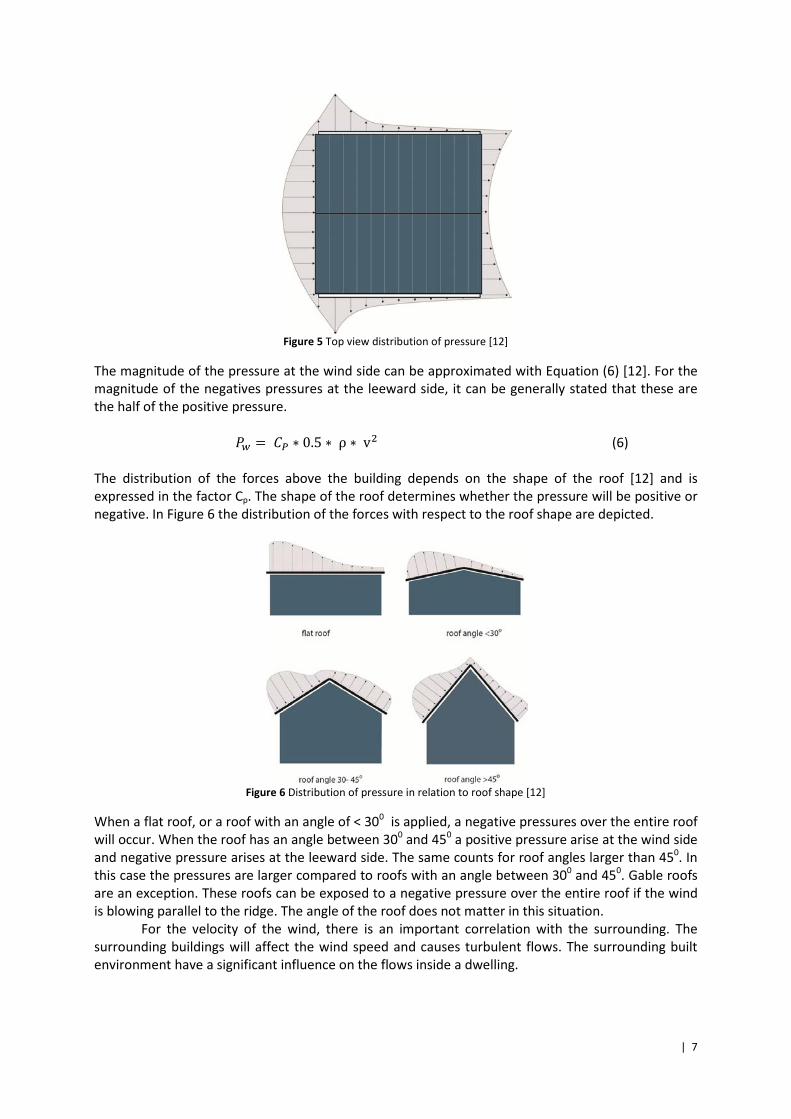
Wind impact
The wind speed can have a significant influence on the on how gases flows within a building during a
fire [11, 12]. In practice, it can be observed that no smoke and gases escape from the building at the
façade were the wind is blowing on. An indication of the distribution of pressures around a dwelling
is depicted in Figures 5 and 6.
| 7
Figure 5 Top view distribution of pressure [12]
The magnitude of the pressure at the wind side can be approximated with Equation (6) [12]. For the
magnitude of the negatives pressures at the leeward side, it can be generally stated that these are
the half of the positive pressure.
�- = ./ ∗ 0.5 ∗ ρ ∗ v� (6)
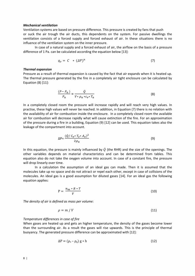
The distribution of the forces above the building depends on the shape of the roof [12] and is
expressed in the factor Cp. The shape of the roof determines whether the pressure will be positive or
negative. In Figure 6 the distribution of the forces with respect to the roof shape are depicted.
Figure 6 Distribution of pressure in relation to roof shape [12]
When a flat roof, or a roof with an angle of < 300 is applied, a negative pressures over the entire roof
will occur. When the roof has an angle between 300 and 45
0 a positive pressure arise at the wind side
and negative pressure arises at the leeward side. The same counts for roof angles larger than 450. In
this case the pressures are larger compared to roofs with an angle between 300 and 45
0. Gable roofs
are an exception. These roofs can be exposed to a negative pressure over the entire roof if the wind
is blowing parallel to the ridge. The angle of the roof does not matter in this situation.
For the velocity of the wind, there is an important correlation with the surrounding. The
surrounding buildings will affect the wind speed and causes turbulent flows. The surrounding built
environment have a significant influence on the flows inside a dwelling.
8 |
Mechanical ventilation
Ventilation systems are based on pressure difference. This pressure is created by fans that push
or suck the air trough the air ducts, this dependents on the system. For passive dwellings the
ventilation consists of a forced supply and forced exhaust of air. In these situations there is no
influence of the ventilation system on the inner pressure.
In case of a natural supply and a forced exhaust of air, the airflow on the basis of a pressure
difference of 1 Pa. can be calculated according the equation below [13]:
3 = . ∗ (4�)� (7)
Thermal expansion
Pressure as a result of thermal expansion is caused by the fact that air expands when it is heated up.
The thermal pressure generated by the fire in a completely air tight enclosure can be calculated by
Equation (8) [11]:
(/5/*)/* =
6�7∗�*∗89∗,* (8)
In a completely closed room the pressure will increase rapidly and will reach very high values. In
practise, these high values will never be reached. In addition, in Equation (7) there is no relation with
the availability of air for combustion inside the enclosure. In a completely closed room the available
air for combustion will decrease rapidly what will cause extinction of the fire. For an approximation
of the pressure during a fire in a building, Equation (9) [12] can be used. This equation takes also the
leakage of the compartment into account.
ΔP= (6� /;9∗,<∗'<)�
��* (9)
In this equation, the pressure is mainly influenced by �� (the RHR) and the size of the openings. The
other variables depends on material characteristics and can be determined from tables. This
equation also do not take the oxygen volume into account. In case of a constant fire, the pressure
will drop linearly over time.
In a calculation the assumption of an ideal gas can made. Then it is assumed that the
molecules take up no space and do not attract or repel each other, except in case of collisions of the
molecules. An ideal gas is a good assumption for diluted gases [14]. For an ideal gas the following
equation applies:
P=�=∗>∗,7 (10)
The density of air is defined as mass per volume:
? = @/A (11)
Temperature differences in case of fire
When gases are heated up and gets an higher temperature, the density of the gases become lower
than the surrounding air. As a result the gases will rise upwards. This is the principle of thermal
buoyancy. The generated pressure difference can be approximated with [12]:
ΔP = (ρa – ρg) g ∗ h (12)
| 9
Or in terms of temperature:
ΔP = 353D �,* − �,+ E g ∗ h (13)
In Equations (12) and (13) the variable h represents the height of the hot smoke layer. In an ideal
situations there is a strict separation between the upper and lower layer. However, the practice will
be more complicated as flows will arise due to oxygen supplies by leakage areas for example.
3.2 Modern dwellings
As mentioned in the literature study [15], little research is done with regard to the pressure build up
during fire in well insulated and airtight dwellings. However, in the field of the nuclear industry
extensive research is done to investigate the pressure increase in confined enclosures in case of fire
[16, 17, 18, 19]. Although the research focus on a single aspect, the involved variables can be roughly
divided into three groups of parameters [16]:
• RHR
• (Thermal) properties of the compartment
• Ventilation network and air flow resistance
To which extent modern dwellings and passive dwellings can be compared with the situations
described in the literature study depends on the characteristics of the dwelling. For passive dwellings
the characteristics are quantified during the design phase but are also measured before the
completion of the dwelling, and can therefore provides valuable information about practical
situations. The concept can therefore be the basis for the parameter study whereby statements
about modern dwellings in general can be abstracted by changing the values of the parameters. The
passive house concept defines the boundary conditions for the (thermal) properties of the
compartment and can be defined as follows [20, 21]:
• The annual primary energy demand is not more than 120 kWh/m2 per year
• The annual heating demand for space heating is not more than 15 kWh/m2per year
• The maximum infiltration rate is n = 0.6 h-1
. This can be translated into a qv;10 value of
0.15 dm3/s.m
2 (Appendix 1)
• The frequency of overheating (inner temperature of > 25 0C) is at most 10%
The boundary conditions for an ‘average’ dwelling are expected to lie between the passive dwellings
and the minimum prescribed amount of insulation in the building code and will have a significant
impact on the fire behaviour.
The passive house concept provides a guideline for this research as it will always meet the
requirements of the third category and make therefore possible to make statements, in contradiction
to modern buildings. For that reason, the passive house concept will be used as a starting point to
make statements about the fire safety of modern dwellings. In order to make statements about well
insulated and airtight dwellings, a risk based approach will be used in Chapter 4 “Computational
approach”.
3.3 Closure
In a dwelling, there are always pressure differences as a result of the temperature difference
between inside and outside the dwelling, wind impact and the mechanical ventilation. Although they
may have an influence on the pressure build-up during fire, they are hard to simulate and are
characterized by large deviations. However, it is expected that they will be subordinate to pressure
differences which are generated by thermal expansion in case of fire. To that end, these factors are
excluded and the research will focus only on the pressure differences generated by the fire. The
provided equations in this chapter can be used as a guideline for the magnitude, and so the influence
of these factors.

10 |
| 11
4. Computational approach
In this chapter a computational approach of the problem is made. The goal is to identify and visualize
the fire scenario which can be expected during a fire in a well insulated and airtight dwelling, in order
to predict the pressure difference within the enclosure. Although the focus is on the passive house
standard, also less good insulated dwellings will be examined as it gives an indication of the pressure
build-up in more common dwellings. The standards of the passive house concept provides quantified
characteristics and are therefore a good starting point for the research. In this chapter, Ozone will be
used to provide the simulations. In the first paragraph the input parameters, values and assumptions
will be accounted and in the second paragraph the fire scenario will be determined. In the third
paragraph the uncertainty will be considered and finally, a sensitivity analysis over the identified
parameters from the literature study will be carried out and a connection with practical situations is
made.
4.1 Input Parameters
Compartment
For the fire room an enclosure with the internal dimensions of 4.0 x 5.0 x 2.6 meter (w x l x h) is
maintained. This enclosure is not representing a specific function and the size is chosen arbitrary. But
the dimensions are chosen such that the enclosure could represent a bedroom or kitchen, the rooms
in a dwelling wherein a fire mostly occurs [9]. In the model, the situation is assumed to be adiabatic
in order to exclude the influence of the enclosure. The influence of the enclosure will be investigated
in a later stage, in the sensitiveness analysis. The entire Ozone input and made assumptions can be
found in Appendix 2.
Air-tightness of the compartment
Ozone assumes that the input geometry is completely air-tight. Therefore the infiltration must be
defined by hand and must be entered as a constant opening in de Ozone model. Conform the passive
house standard, the maximum amount of infiltration is 0.15 dm3/s.m
2, at ΔP = 10 Pa. So the
maximum infiltration in the fire room of 20 m2 at a pressure difference of 10 Pa. must be 3.0 dm
3/s.
However, the amount of infiltration of the passive standard applies only to the facades. As the fire
room is a part of a larger dwelling, the inner walls will have a lower air tightness as the outer walls as
they do not have to meet the requirements for the amount of infiltration.
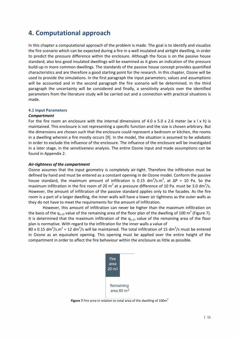
However, this amount of infiltration can never be higher than the maximum infiltration on
the basis of the qv;10 value of the remaining area of the floor plan of the dwelling of 100 m2 (Figure 7).
It is determined that the maximum infiltration of the qv;10 value of the remaining area of the floor
plan is normative. With regard to the infiltration for the inner walls a value of
80 x 0.15 dm3/s.m
2 = 12 dm
3/s will be maintained. The total infiltration of 15 dm
3/s must be entered
in Ozone as an equivalent opening. This opening must be applied over the entire height of the
compartment in order to affect the fire behaviour within the enclosure as little as possible.
Figure 7 Fire area in relation to total area of the dwelling of 100m
2
12 |
The equivalent opening in Ozone, due to air-infiltration, can be calculated according to Equation (14),
with a pressure difference of 10 Pa:
FG;�I = J9;KLI.MNN∗√�I (14)
However, when the pressure difference is significantly higher it make sense that a higher inner
pressure leads to a larger air flow through the slit whereby these deviations become too large to
ignore. Therefore, for this specific situation a correction must be applied. Equations (15) and (16) [22]
are the basic equations needed for the correction:
FG;P = ;∗Q��III∗�� (15)
3 ;P =∑. ∗(4S)� (16)
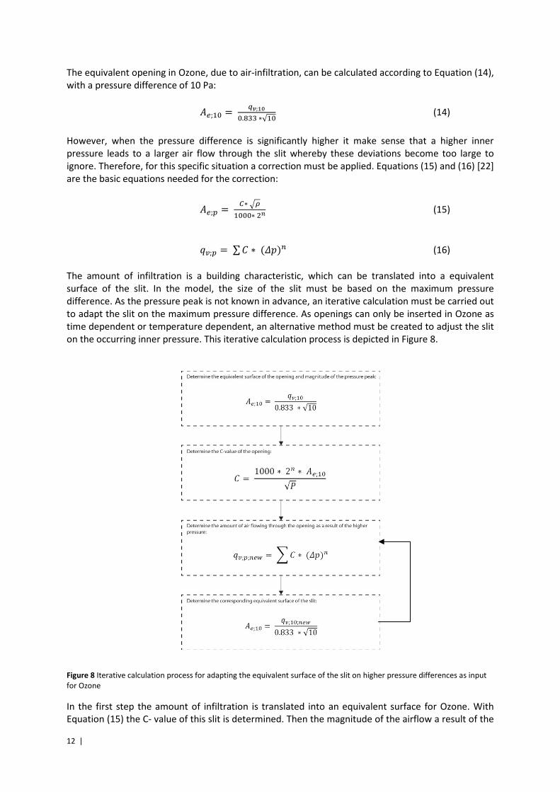
The amount of infiltration is a building characteristic, which can be translated into a equivalent
surface of the slit. In the model, the size of the slit must be based on the maximum pressure
difference. As the pressure peak is not known in advance, an iterative calculation must be carried out
to adapt the slit on the maximum pressure difference. As openings can only be inserted in Ozone as
time dependent or temperature dependent, an alternative method must be created to adjust the slit
on the occurring inner pressure. This iterative calculation process is depicted in Figure 8.
Figure 8 Iterative calculation process for adapting the equivalent surface of the slit on higher pressure differences as input
for Ozone
In the first step the amount of infiltration is translated into an equivalent surface for Ozone. With
Equation (15) the C- value of this slit is determined. Then the magnitude of the airflow a result of the
| 13
higher pressure can be calculated with Equation (16). In the last step, this airflow must be translated
back into an equivalent surface of the slit which can be entered in Ozone.
By calculating the equivalent surface for a number of pressure intervals, the slit can be
adjusted on the outcome of the pressure peak of Ozone.
With regard to determining the C- value a remark must be placed. When the size of the equivalent
opening is changed, this value will also change. In order to simplify the approximation, the amount of
variables is limited to one. Therefore, the C- value is considered to be constant. In order to overcome
this shortcoming and the shortcoming of the flow exponent n ≠ 0.5, also other simulation software
like CONTAM is considered. However, there is no simulation software currently available which
contains the possibility to apply a RHR curve as temperature input and an air infiltration model as
well.
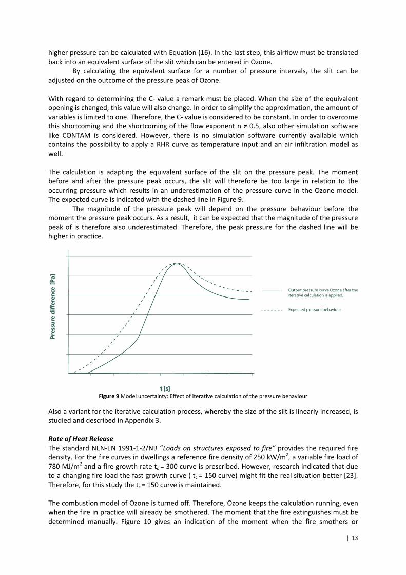
The calculation is adapting the equivalent surface of the slit on the pressure peak. The moment
before and after the pressure peak occurs, the slit will therefore be too large in relation to the
occurring pressure which results in an underestimation of the pressure curve in the Ozone model.
The expected curve is indicated with the dashed line in Figure 9.
The magnitude of the pressure peak will depend on the pressure behaviour before the
moment the pressure peak occurs. As a result, it can be expected that the magnitude of the pressure
peak of is therefore also underestimated. Therefore, the peak pressure for the dashed line will be
higher in practice.
Figure 9 Model uncertainty: Effect of iterative calculation of the pressure behaviour
Also a variant for the iterative calculation process, whereby the size of the slit is linearly increased, is
studied and described in Appendix 3.
Rate of Heat Release
The standard NEN-EN 1991-1-2/NB “Loads on structures exposed to fire” provides the required fire
density. For the fire curves in dwellings a reference fire density of 250 kW/m2, a variable fire load of
780 MJ/m2 and a fire growth rate tc = 300 curve is prescribed. However, research indicated that due
to a changing fire load the fast growth curve ( tc = 150 curve) might fit the real situation better [23].
Therefore, for this study the tc = 150 curve is maintained.
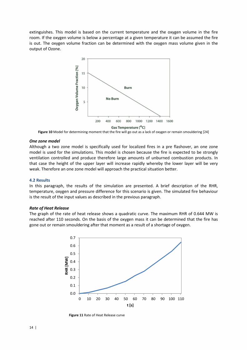
The combustion model of Ozone is turned off. Therefore, Ozone keeps the calculation running, even
when the fire in practice will already be smothered. The moment that the fire extinguishes must be
determined manually. Figure 10 gives an indication of the moment when the fire smothers or
14 |
extinguishes. This model is based on the current temperature and the oxygen volume in the fire
room. If the oxygen volume is below a percentage at a given temperature it can be assumed the fire
is out. The oxygen volume fraction can be determined with the oxygen mass volume given in the
output of Ozone.
Figure 10 Model for determining moment that the fire will go out as a lack of oxygen or remain smouldering [24]
One zone model
Although a two zone model is specifically used for localized fires in a pre flashover, an one zone
model is used for the simulations. This model is chosen because the fire is expected to be strongly
ventilation controlled and produce therefore large amounts of unburned combustion products. In
that case the height of the upper layer will increase rapidly whereby the lower layer will be very
weak. Therefore an one zone model will approach the practical situation better.
4.2 Results
In this paragraph, the results of the simulation are presented. A brief description of the RHR,
temperature, oxygen and pressure difference for this scenario is given. The simulated fire behaviour
is the result of the input values as described in the previous paragraph.
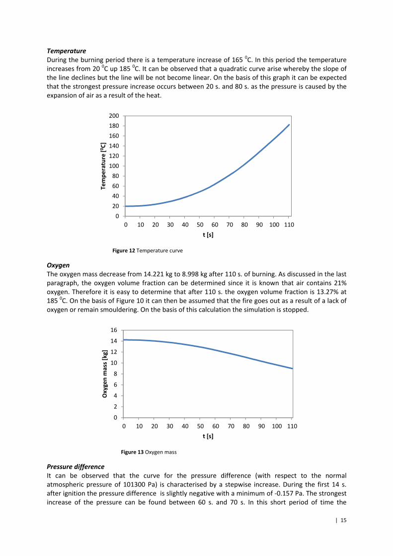
Rate of Heat Release
The graph of the rate of heat release shows a quadratic curve. The maximum RHR of 0.644 MW is
reached after 110 seconds. On the basis of the oxygen mass it can be determined that the fire has
gone out or remain smouldering after that moment as a result of a shortage of oxygen.
Figure 11 Rate of Heat Release curve
0.0
0.1
0.2
0.3
0.4
0.5
0.6
0.7
0 10 20 30 40 50 60 70 80 90 100 110
RH
R [
MW
]
t [s]
| 15
Temperature
During the burning period there is a temperature increase of 165 0C. In this period the temperature
increases from 20 0C up 185
0C. It can be observed that a quadratic curve arise whereby the slope of
the line declines but the line will be not become linear. On the basis of this graph it can be expected
that the strongest pressure increase occurs between 20 s. and 80 s. as the pressure is caused by the
expansion of air as a result of the heat.
Figure 12 Temperature curve
Oxygen
The oxygen mass decrease from 14.221 kg to 8.998 kg after 110 s. of burning. As discussed in the last
paragraph, the oxygen volume fraction can be determined since it is known that air contains 21%
oxygen. Therefore it is easy to determine that after 110 s. the oxygen volume fraction is 13.27% at
185 0C. On the basis of Figure 10 it can then be assumed that the fire goes out as a result of a lack of
oxygen or remain smouldering. On the basis of this calculation the simulation is stopped.
Figure 13 Oxygen mass
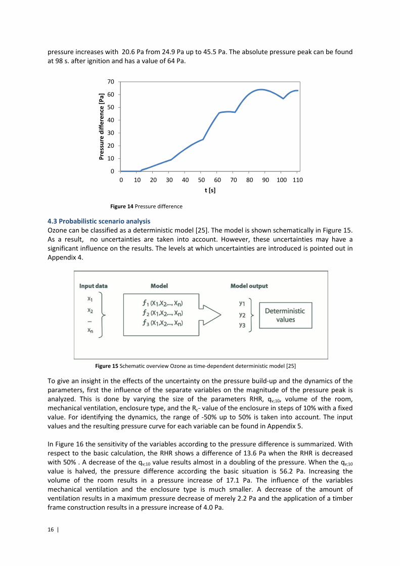
Pressure difference
It can be observed that the curve for the pressure difference (with respect to the normal
atmospheric pressure of 101300 Pa) is characterised by a stepwise increase. During the first 14 s.
after ignition the pressure difference is slightly negative with a minimum of -0.157 Pa. The strongest
increase of the pressure can be found between 60 s. and 70 s. In this short period of time the
0
20
40
60
80
100
120
140
160
180
200
0 10 20 30 40 50 60 70 80 90 100 110
Te
mp
era
ture
[0C
]
t [s]
0
2
4
6
8
10
12
14
16
0 10 20 30 40 50 60 70 80 90 100 110
Ox
yg
en
ma
ss [
kg
]
t [s]
16 |
pressure increases with 20.6 Pa from 24.9 Pa up to 45.5 Pa. The absolute pressure peak can be found
at 98 s. after ignition and has a value of 64 Pa.
Figure 14 Pressure difference
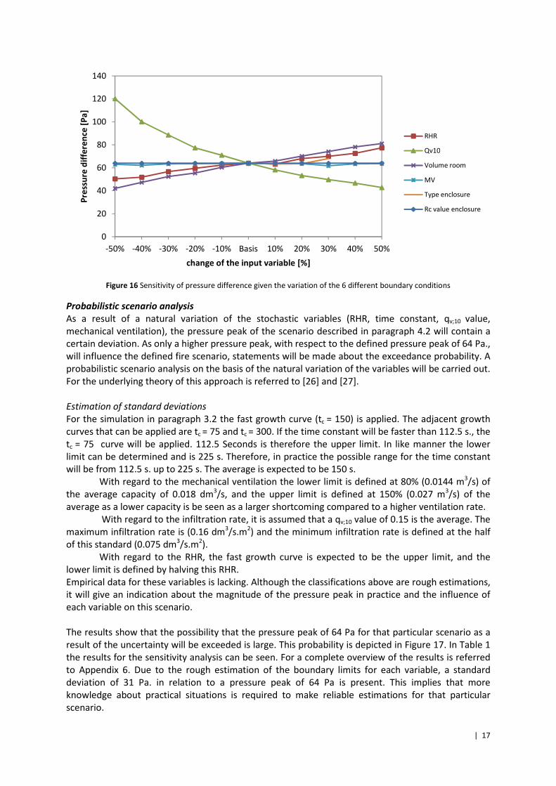
4.3 Probabilistic scenario analysis
Ozone can be classified as a deterministic model [25]. The model is shown schematically in Figure 15.
As a result, no uncertainties are taken into account. However, these uncertainties may have a
significant influence on the results. The levels at which uncertainties are introduced is pointed out in
Appendix 4.
Figure 15 Schematic overview Ozone as time-dependent deterministic model [25]
To give an insight in the effects of the uncertainty on the pressure build-up and the dynamics of the
parameters, first the influence of the separate variables on the magnitude of the pressure peak is
analyzed. This is done by varying the size of the parameters RHR, qv;10, volume of the room,
mechanical ventilation, enclosure type, and the Rc- value of the enclosure in steps of 10% with a fixed
value. For identifying the dynamics, the range of -50% up to 50% is taken into account. The input
values and the resulting pressure curve for each variable can be found in Appendix 5.
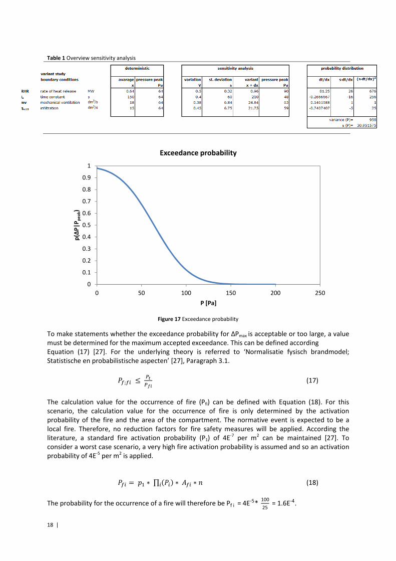
In Figure 16 the sensitivity of the variables according to the pressure difference is summarized. With
respect to the basic calculation, the RHR shows a difference of 13.6 Pa when the RHR is decreased
with 50% . A decrease of the qv;10 value results almost in a doubling of the pressure. When the qv;10
value is halved, the pressure difference according the basic situation is 56.2 Pa. Increasing the
volume of the room results in a pressure increase of 17.1 Pa. The influence of the variables
mechanical ventilation and the enclosure type is much smaller. A decrease of the amount of
ventilation results in a maximum pressure decrease of merely 2.2 Pa and the application of a timber
frame construction results in a pressure increase of 4.0 Pa.
0
10
20
30
40
50
60
70
0 10 20 30 40 50 60 70 80 90 100 110
Pre
ssu
re d
iffe
ren
ce [
Pa
]
t [s]
| 17
Figure 16 Sensitivity of pressure difference given the variation of the 6 different boundary conditions
Probabilistic scenario analysis
As a result of a natural variation of the stochastic variables (RHR, time constant, qv;10 value,
mechanical ventilation), the pressure peak of the scenario described in paragraph 4.2 will contain a
certain deviation. As only a higher pressure peak, with respect to the defined pressure peak of 64 Pa.,
will influence the defined fire scenario, statements will be made about the exceedance probability. A
probabilistic scenario analysis on the basis of the natural variation of the variables will be carried out.
For the underlying theory of this approach is referred to [26] and [27].
Estimation of standard deviations
For the simulation in paragraph 3.2 the fast growth curve (tc = 150) is applied. The adjacent growth
curves that can be applied are tc = 75 and tc = 300. If the time constant will be faster than 112.5 s., the
tc = 75 curve will be applied. 112.5 Seconds is therefore the upper limit. In like manner the lower
limit can be determined and is 225 s. Therefore, in practice the possible range for the time constant
will be from 112.5 s. up to 225 s. The average is expected to be 150 s.
With regard to the mechanical ventilation the lower limit is defined at 80% (0.0144 m3/s) of
the average capacity of 0.018 dm3/s, and the upper limit is defined at 150% (0.027 m
3/s) of the
average as a lower capacity is be seen as a larger shortcoming compared to a higher ventilation rate.
With regard to the infiltration rate, it is assumed that a qv;10 value of 0.15 is the average. The
maximum infiltration rate is (0.16 dm3/s.m
2) and the minimum infiltration rate is defined at the half
of this standard (0.075 dm3/s.m
2).
With regard to the RHR, the fast growth curve is expected to be the upper limit, and the
lower limit is defined by halving this RHR.
Empirical data for these variables is lacking. Although the classifications above are rough estimations,
it will give an indication about the magnitude of the pressure peak in practice and the influence of
each variable on this scenario.
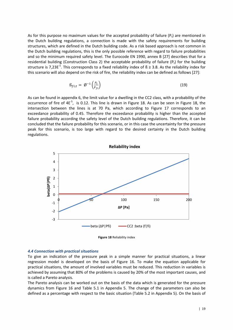
The results show that the possibility that the pressure peak of 64 Pa for that particular scenario as a
result of the uncertainty will be exceeded is large. This probability is depicted in Figure 17. In Table 1
the results for the sensitivity analysis can be seen. For a complete overview of the results is referred
to Appendix 6. Due to the rough estimation of the boundary limits for each variable, a standard
deviation of 31 Pa. in relation to a pressure peak of 64 Pa is present. This implies that more
knowledge about practical situations is required to make reliable estimations for that particular
scenario.
0
20
40
60
80
100
120
140
-50% -40% -30% -20% -10% Basis 10% 20% 30% 40% 50%
Pre
ssu
re d
iffe
ren
ce [
Pa
]
change of the input variable [%]
RHR
Qv10
Volume room
MV
Type enclosure
Rc value enclosure
18 |
Table 1 Overview sensitivity analysis
Sdsds
Figure 17 Exceedance probability
To make statements whether the exceedance probability for ΔPmax is acceptable or too large, a value
must be determined for the maximum accepted exceedance. This can be defined according
Equation (17) [27]. For the underlying theory is referred to ‘Normalisatie fysisch brandmodel;
Statistische en probabilistische aspecten’ [27], Paragraph 3.1.
�T;TU ≤ /W/XY (17)
The calculation value for the occurrence of fire (Pfi) can be defined with Equation (18). For this
scenario, the calculation value for the occurrence of fire is only determined by the activation
probability of the fire and the area of the compartment. The normative event is expected to be a
local fire. Therefore, no reduction factors for fire safety measures will be applied. According the
literature, a standard fire activation probability (P1) of 4E-7
per m2 can be maintained [27]. To
consider a worst case scenario, a very high fire activation probability is assumed and so an activation
probability of 4E-5
per m2 is applied.
�TU =S� ∗ ∏ (�U) ∗ FTU ∗ [U (18)
The probability for the occurrence of a fire will therefore be Pfi=4E-5* 100
25=1.6E-4.
0
0.1
0.2
0.3
0.4
0.5
0.6
0.7
0.8
0.9
1
0 50 100 150 200 250
p(Δ
P|
Pp
ea
k)
P [Pa]
Exceedance probability
| 19
As for this purpose no maximum values for the accepted probability of failure (Pt) are mentioned in
the Dutch building regulations, a connection is made with the safety requirements for building
structures, which are defined in the Dutch building code. As a risk based approach is not common in
the Dutch building regulations, this is the only possible reference with regard to failure probabilities
and so the minimum required safety level. The Eurocode EN 1990, annex B [27] describes that for a
residential building (Construction Class 2) the acceptable probability of failure (Pt) for the building
structure is 7,23E-5
. This corresponds to a fixed reliability index of ß ≥ 3.8. As the reliability index for
this scenario will also depend on the risk of fire, the reliability index can be defined as follows [27]:
ßTU;] = Ø5� D /W/XYE (19)
As can be found in appendix 6, the limit value for a dwelling in the CC2 class, with a probability of the
occurrence of fire of 4E-5
, is 0.12. This line is drawn in Figure 18. As can be seen in Figure 18, the
intersection between the lines is at 70 Pa, which according to Figure 17 corresponds to an
exceedance probability of 0.45. Therefore the exceedance probability is higher than the accepted
failure probability according the safety level of the Dutch building regulations. Therefore, it can be
concluded that the failure probability for this scenario, or in this case the uncertainty for the pressure
peak for this scenario, is too large with regard to the desired certainty in the Dutch building
regulations.
Figure 18 Reliability index
4.4 Connection with practical situations
To give an indication of the pressure peak in a simple manner for practical situations, a linear
regression model is developed on the basis of Figure 16. To make the equation applicable for
practical situations, the amount of involved variables must be reduced. This reduction in variables is
achieved by assuming that 80% of the problems is caused by 20% of the most important causes, and
is called a Pareto analysis.
The Pareto analysis can be worked out on the basis of the data which is generated for the pressure
dynamics from Figure 16 and Table 5.1 in Appendix 5. The change of the parameters can also be
defined as a percentage with respect to the basic situation (Table 5.2 in Appendix 5). On the basis of
-3
-2
-1
0
1
2
3
4
5
0 50 100 150 200
be
ta(Δ
P|
Pfi
)
ΔP [Pa]
Reliability index
beta (ΔP|Pfi) CC2 :beta (f|fi)
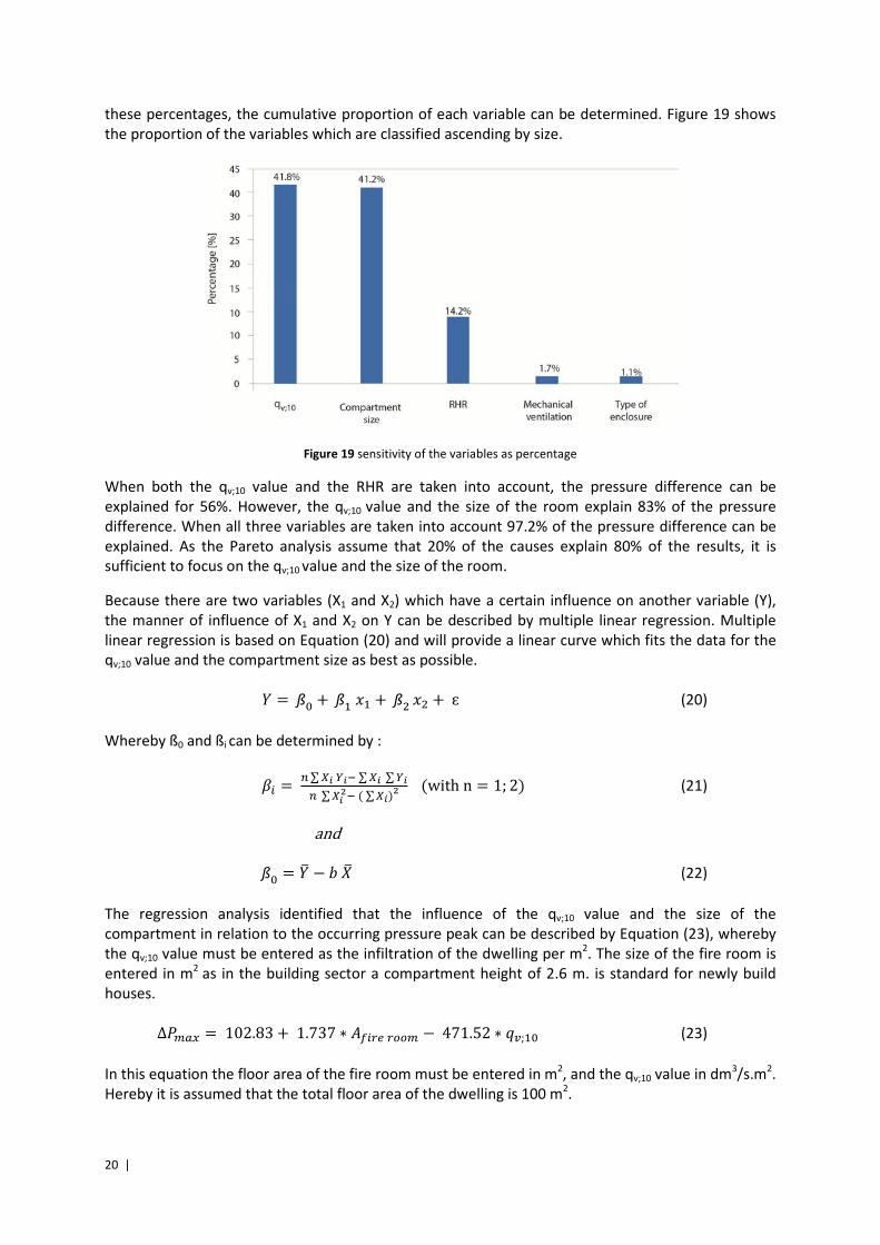
20 |
these percentages, the cumulative proportion of each variable can be determined. Figure 19 shows
the proportion of the variables which are classified ascending by size.
Figure 19 sensitivity of the variables as percentage
When both the qv;10 value and the RHR are taken into account, the pressure difference can be
explained for 56%. However, the qv;10 value and the size of the room explain 83% of the pressure
difference. When all three variables are taken into account 97.2% of the pressure difference can be
explained. As the Pareto analysis assume that 20% of the causes explain 80% of the results, it is
sufficient to focus on the qv;10 value and the size of the room.
Because there are two variables (X1 and X2) which have a certain influence on another variable (Y),
the manner of influence of X1 and X2 on Y can be described by multiple linear regression. Multiple
linear regression is based on Equation (20) and will provide a linear curve which fits the data for the
qv;10 value and the compartment size as best as possible.
_ = ßI +ß�`� +ß�`� + ɛ (20)
Whereby ß0 and ßi can be determined by :
bU = �∑cYdY5∑cY ∑ dY�∑cY�5(∑cY)�(withn = 1; 2) (21)
and
ßI = _k − lmk (22)
The regression analysis identified that the influence of the qv;10 value and the size of the
compartment in relation to the occurring pressure peak can be described by Equation (23), whereby
the qv;10 value must be entered as the infiltration of the dwelling per m2. The size of the fire room is
entered in m2
as in the building sector a compartment height of 2.6 m. is standard for newly build
houses.
Δ�nop = 102.83 + 1.737 ∗ FTUsGsttn − 471.52 ∗ 3 ;�I (23)
In this equation the floor area of the fire room must be entered in m2, and the qv;10 value in dm
3/s.m
2.
Hereby it is assumed that the total floor area of the dwelling is 100 m2.
| 21
To which extent this curve fits to the data from Table 2 is indicated by the adjusted least
square coefficient (R2
adj), this value is 0.887 and can be calculated on the basis of Equation (24). As
this value is high, it means that the developed equation fits the data from Figure 16 very well. The
fact that the R2 - value and the R
2adj in Appendix 7 are close to each other is caused by the small
sample size. As the F- value of the results is 1.14E-09, statements can be made based on a 98%
confidence level with regard to the data of Figure 16. An overview of the results can be found in
Appendix 7.
vowx� = yy<zz{z/(�5P)yyW{W/(�5�) (24)
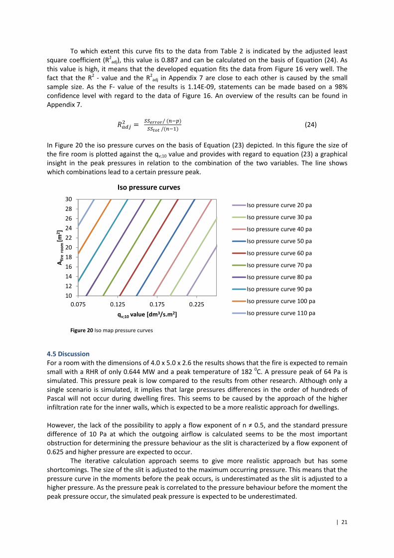
In Figure 20 the iso pressure curves on the basis of Equation (23) depicted. In this figure the size of
the fire room is plotted against the qv;10 value and provides with regard to equation (23) a graphical
insight in the peak pressures in relation to the combination of the two variables. The line shows
which combinations lead to a certain pressure peak.
Figure 20 Iso map pressure curves
4.5 Discussion
For a room with the dimensions of 4.0 x 5.0 x 2.6 the results shows that the fire is expected to remain
small with a RHR of only 0.644 MW and a peak temperature of 182 0C. A pressure peak of 64 Pa is
simulated. This pressure peak is low compared to the results from other research. Although only a
single scenario is simulated, it implies that large pressures differences in the order of hundreds of
Pascal will not occur during dwelling fires. This seems to be caused by the approach of the higher
infiltration rate for the inner walls, which is expected to be a more realistic approach for dwellings.
However, the lack of the possibility to apply a flow exponent of n ≠ 0.5, and the standard pressure
difference of 10 Pa at which the outgoing airflow is calculated seems to be the most important
obstruction for determining the pressure behaviour as the slit is characterized by a flow exponent of
0.625 and higher pressure are expected to occur.
The iterative calculation approach seems to give more realistic approach but has some
shortcomings. The size of the slit is adjusted to the maximum occurring pressure. This means that the
pressure curve in the moments before the peak occurs, is underestimated as the slit is adjusted to a
higher pressure. As the pressure peak is correlated to the pressure behaviour before the moment the
peak pressure occur, the simulated peak pressure is expected to be underestimated.
10
12
14
16
18
20
22
24
26
28
30
0.075 0.125 0.175 0.225
Afi
re r
oo
m [
m2]
qv;10 value [dm3/s.m2]
Iso pressure curves
Iso pressure curve 20 pa
Iso pressure curve 30 pa
Iso pressure curve 40 pa
Iso pressure curve 50 pa
Iso pressure curve 60 pa
Iso pressure curve 70 pa
Iso pressure curve 80 pa
Iso pressure curve 90 pa
Iso pressure curve 100 pa
Iso pressure curve 110 pa
22 |
Moreover, it is possible that the calculated C- value, which is determined for the iterative
calculation process, is not accurate enough as the C- value of the opening varies during the fire.
The results for this particular scenario cannot exclude that high pressures might occur as some input
values can be considered as a result of a lack of knowledge about practical situations.
The used qv;10 value, for example, is the minimum level for a passive dwellings. An enclosure
which is 50% more airtight will lead to a pressure peak of 120 Pa, which is an increase of 87.8%.
Moreover, the volume of the enclosure may vary in practice and it expected to lead to a higher
pressure peak. With the common open floor plans for dwellings it can be expected that the chosen
geometry is a best case scenario as a larger floor plan leads to higher pressure peaks.
On the other hand, the enclosure in the simulations is assumed to be adiabatic and the
simulation is based on the fast growth curve instead of the according the standard
NEN-EN 1991-1-2/NB prescribed medium growth curve. Moreover, no coincidental factors as opened
doors and windows are incorporated.
The probabilistic scenario analysis is used to overcome these uncertainties. As the building
code is characterized by prescriptive rules instead of a probabilistic approach, no minimum level of
certainty is defined. To that end, as indication for the minimum required level of safety the failure
probability for building structures is maintained. This probabilistic approach makes it only possible to
make statements about the described scenario.
To give an indication of the magnitude of the pressure peak at a higher level, the multiple linear
regression model is developed. This equation is only applicable for practical situations within the
range of -50% up to +50% with respect to the variables of the above described enclosure. Caution is
required when results are extrapolated as this might results in larger deviations.
4.6 Conclusion
As a result of the incorporated fixed flow exponent n = 0.5 and a pressure difference of 10 Pa.
whereby the magnitude of the airflow is calculated in Ozone, the pressure behaviour in passive
dwellings cannot be simulated accurately. To that end, the size of the slit which represents the
infiltration of a passive dwellings in the model is adapted on the calculation method of Ozone.
An enclosure which meets the requirements of a passive house with the dimensions of
4.0 x 5.0 x 2.6 m (l x w x h) is modelled. These dimensions are arbitrary but are chosen such that it
could represent a small living room or a large bedroom, the rooms in which a fire mostly occur. In the
model it is assumed that the enclosure is adiabatic. The enclosure is expected to be a part of a
dwelling of 100 m2 which results in a higher amount of infiltration for the inner walls.
The results for this scenario indicates that the fire remains small with a RHR of 0.644 MW. The fire is
expected to spontaneously go out as a result of a lack of oxygen after 120 s. During these two
minutes the temperature increases to 182 0C and a pressure peak of 64 Pa is reached after 98 s.
Although it can be assumed that this pressure is underestimated as a result of the size of the slit, it
can be concluded that a pressure increase in the order of hundreds of Pascal is not obvious for this
scenario. Nevertheless, it can be stated that the occurring pressure is higher compared to fires in
conventional dwellings. Coincidental factors like opened doors and windows are not included in the
simulation. Therefore, a wide range of scenarios is possible.
As a result of natural variation for the input parameters (RHR, time constant, qv;10 value and the
mechanical ventilation) the standard deviation for the pressure peak is 31 Pa. Taking into account the
maximum failure probability for building structures from the building code, it must be concluded that
the exceedance probability for the pressure peak is too large. This is caused by a lack of knowledge
about the values of the parameters in practical situations.
| 23
The qv;10 value and the compartment size affects the magnitude of the pressure peak at most. To that
end, these to variables are used for a multiple linear regression model to predict the magnitude of
the pressure peak. Within a range of +/- 50% with respect to the initial values for the qv;10 value and
the compartment size the magnitude of the pressure peak can be estimated with the following
equation:
4�nop = 102.83 + 1.737 ∗ FTUsGsttn − 471.52 ∗ 3 ;�I
In this equation the floor area of the fire room must be entered in m2, and the qv;10 value in dm
3/s.m
2.
Hereby it is assumed that the total floor area of the dwelling is 100 m2.

24 |
| 25
5. Experimental approach
Purpose of the experiments is on the one hand identifying if high pressures can occur during fire in
well insulated and airtight dwellings and on the other hand generating data in order to validate the
simulations as conducted in Chapter 4 ‘Computational approach’. To this end, real scale fire
experiments are conducted at the Troned (Trainings- en Oefencentrum brandweer Oost-Nederland)
on the Twente Safety Campus in Enschede. The Safety campus provides the ability to generate data
by conducting fire tests under realistic conditions. In this chapter, the experimental design will be
described and the results of the experiments will be described and analyzed. In the discussion the
experimental results will be interpreted and then compared to the preliminary calculations. Then
differences between the calculations and experimental results will be explained and the simulation
models from the preliminary calculations will be fitted subsequently on the experimental results
5.1 Work plan
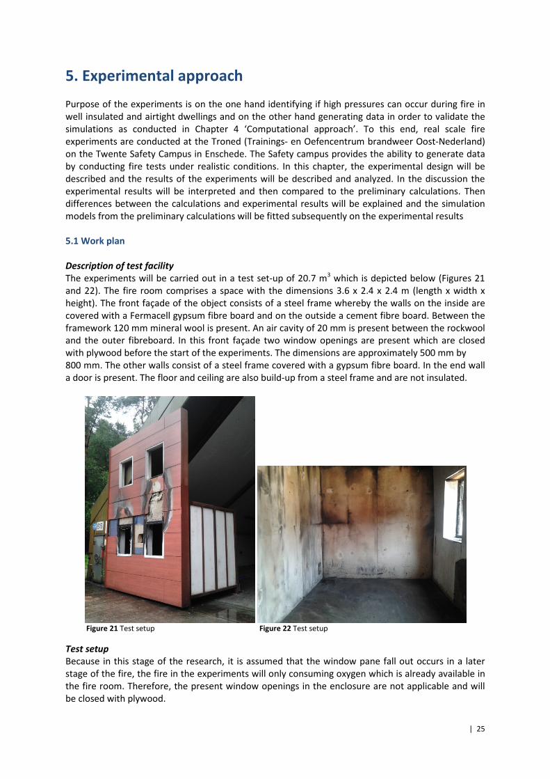
Description of test facility
The experiments will be carried out in a test set-up of 20.7 m3 which is depicted below (Figures 21
and 22). The fire room comprises a space with the dimensions 3.6 x 2.4 x 2.4 m (length x width x
height). The front façade of the object consists of a steel frame whereby the walls on the inside are
covered with a Fermacell gypsum fibre board and on the outside a cement fibre board. Between the
framework 120 mm mineral wool is present. An air cavity of 20 mm is present between the rockwool
and the outer fibreboard. In this front façade two window openings are present which are closed
with plywood before the start of the experiments. The dimensions are approximately 500 mm by
800 mm. The other walls consist of a steel frame covered with a gypsum fibre board. In the end wall
a door is present. The floor and ceiling are also build-up from a steel frame and are not insulated.
Figure 21 Test setup Figure 22 Test setup
Test setup
Because in this stage of the research, it is assumed that the window pane fall out occurs in a later
stage of the fire, the fire in the experiments will only consuming oxygen which is already available in
the fire room. Therefore, the present window openings in the enclosure are not applicable and will
be closed with plywood.
26 |
In the parameter study as described in paragraph 4.3, the influence of six variables on the pressure
build-up in dwelling fires has been identified. It has been found that the level of air-tightness of the
enclosure is one of the main factors which determine the magnitude of the pressure build-up. To this
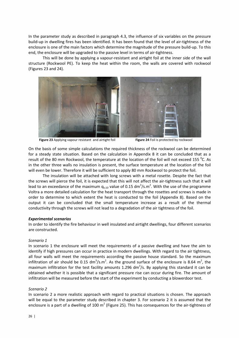
end, the enclosure will be upgraded to the passive level in terms of air-tightness.
This will be done by applying a vapour-resistant and airtight foil at the inner side of the wall
structure (Rockwool PE). To keep the heat within the room, the walls are covered with rockwool
(Figures 23 and 24).
Figure 23 Applying vapour resistant and airtight foil Figure 24 Foil is protected by rockwool
On the basis of some simple calculations the required thickness of the rockwool can be determined
for a steady state situation. Based on the calculation in Appendix 8 it can be concluded that as a
result of the 80 mm Rockwool, the temperature at the location of the foil will not exceed 155 0C. As
in the other three walls no insulation is present, the surface temperature at the location of the foil
will even be lower. Therefore it will be sufficient to apply 80 mm Rockwool to protect the foil.
The insulation will be attached with long screws with a metal rosette. Despite the fact that
the screws will pierce the foil, it is expected that this will not affect the air-tightness such that it will
lead to an exceedance of the maximum qv;10 value of 0.15 dm3/s.m
2. With the use of the programme
Voltra a more detailed calculation for the heat transport through the rosettes and screws is made in
order to determine to which extent the heat is conducted to the foil (Appendix 8). Based on the
output it can be concluded that the small temperature increase as a result of the thermal
conductivity through the screws will not lead to a degradation of the air tightness of the foil.
Experimental scenarios
In order to identify the fire behaviour in well insulated and airtight dwellings, four different scenarios
are constructed.
Scenario 1
In scenario 1 the enclosure will meet the requirements of a passive dwelling and have the aim to
identify if high pressures can occur in practice in modern dwellings. With regard to the air tightness,
all four walls will meet the requirements according the passive house standard. So the maximum
infiltration of air should be 0.15 dm3/s.m
2. As the ground surface of the enclosure is 8.64 m
2, the
maximum infiltration for the test facility amounts 1.296 dm3/s. By applying this standard it can be
obtained whether it is possible that a significant pressure rise can occur during fire. The amount of
infiltration will be measured before the start of the experiment by conducting a blowerdoor test.
Scenario 2
In scenario 2 a more realistic approach with regard to practical situations is chosen. The approach
will be equal to the parameter study described in chapter 3. For scenario 2 it is assumed that the
enclosure is a part of a dwelling of 100 m2 (Figure 25). This has consequences for the air-tightness of
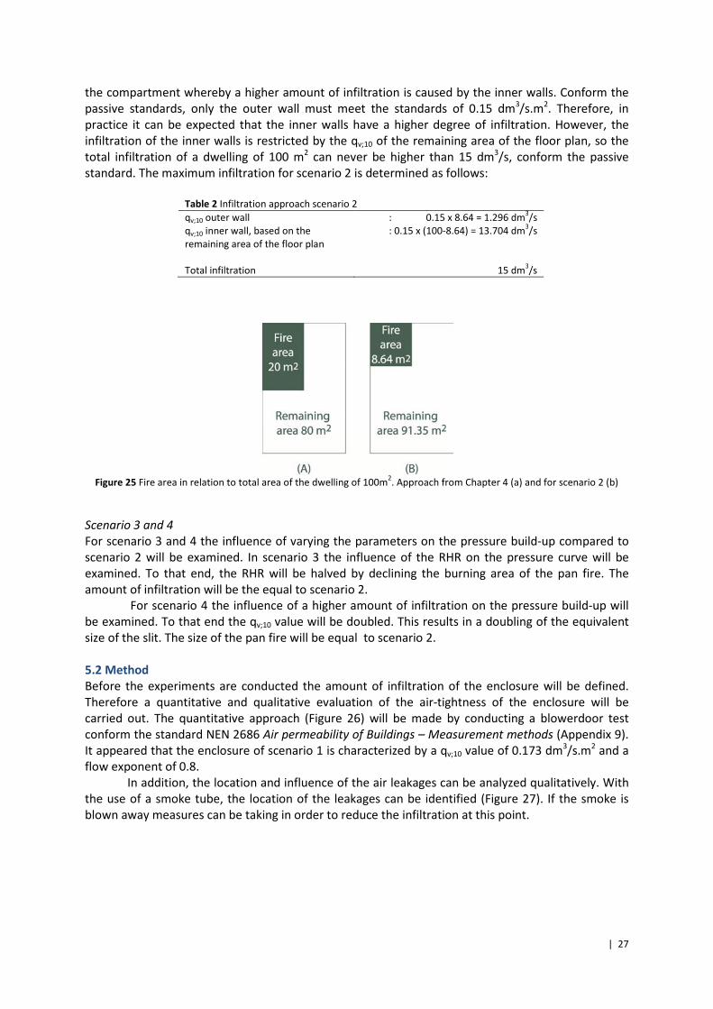
| 27
the compartment whereby a higher amount of infiltration is caused by the inner walls. Conform the
passive standards, only the outer wall must meet the standards of 0.15 dm3/s.m
2. Therefore, in
practice it can be expected that the inner walls have a higher degree of infiltration. However, the
infiltration of the inner walls is restricted by the qv;10 of the remaining area of the floor plan, so the
total infiltration of a dwelling of 100 m2 can never be higher than 15 dm
3/s, conform the passive
standard. The maximum infiltration for scenario 2 is determined as follows:
Table 2 Infiltration approach scenario 2 qv;10 outer wall : 0.15 x 8.64 = 1.296 dm
3/s
qv;10 inner wall, based on the
remaining area of the floor plan
: 0.15 x (100-8.64) = 13.704 dm3/s
Total infiltration 15 dm3/s
Figure 25 Fire area in relation to total area of the dwelling of 100m
2. Approach from Chapter 4 (a) and for scenario 2 (b)
Scenario 3 and 4
For scenario 3 and 4 the influence of varying the parameters on the pressure build-up compared to
scenario 2 will be examined. In scenario 3 the influence of the RHR on the pressure curve will be
examined. To that end, the RHR will be halved by declining the burning area of the pan fire. The
amount of infiltration will be the equal to scenario 2.
For scenario 4 the influence of a higher amount of infiltration on the pressure build-up will
be examined. To that end the qv;10 value will be doubled. This results in a doubling of the equivalent
size of the slit. The size of the pan fire will be equal to scenario 2.
5.2 Method
Before the experiments are conducted the amount of infiltration of the enclosure will be defined.
Therefore a quantitative and qualitative evaluation of the air-tightness of the enclosure will be
carried out. The quantitative approach (Figure 26) will be made by conducting a blowerdoor test
conform the standard NEN 2686 Air permeability of Buildings – Measurement methods (Appendix 9).
It appeared that the enclosure of scenario 1 is characterized by a qv;10 value of 0.173 dm3/s.m
2 and a
flow exponent of 0.8.
In addition, the location and influence of the air leakages can be analyzed qualitatively. With
the use of a smoke tube, the location of the leakages can be identified (Figure 27). If the smoke is
blown away measures can be taking in order to reduce the infiltration at this point.
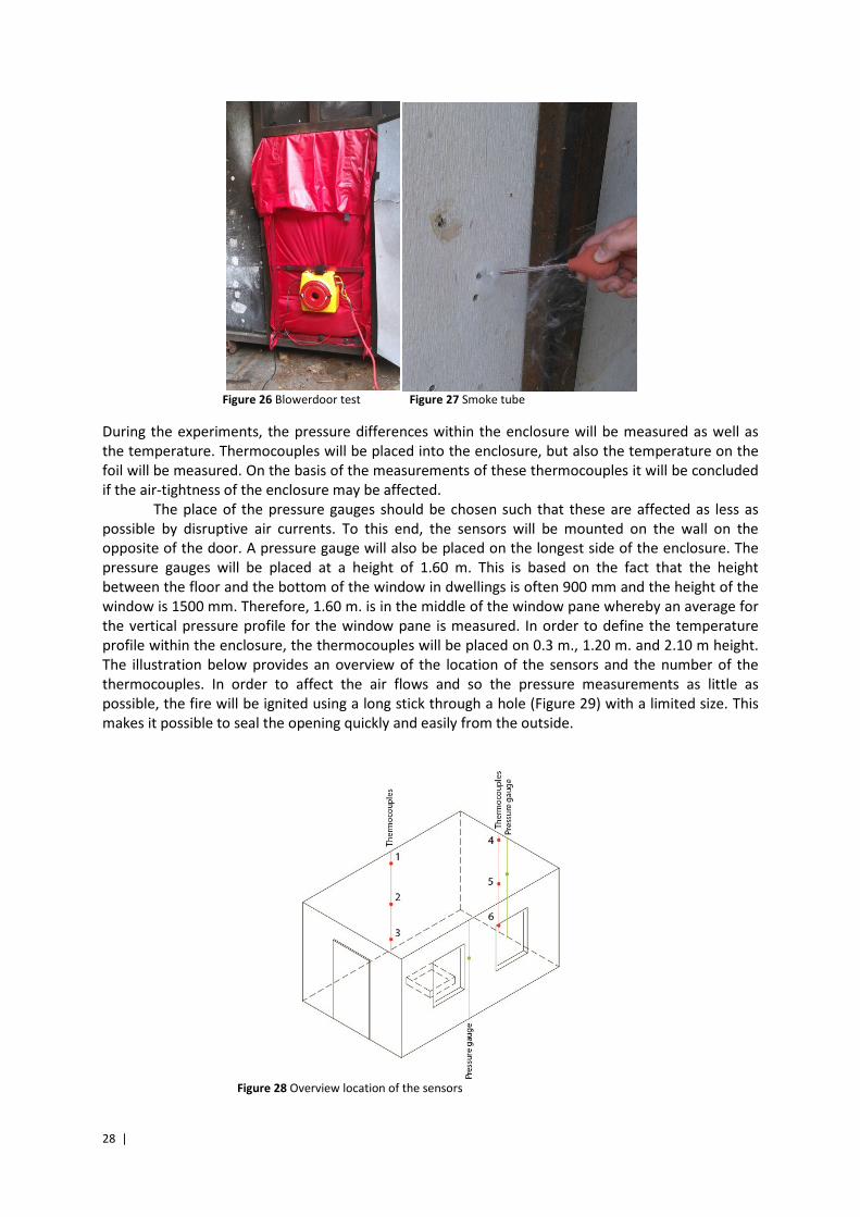
28 |
Figure 26 Blowerdoor test Figure 27 Smoke tube
During the experiments, the pressure differences within the enclosure will be measured as well as
the temperature. Thermocouples will be placed into the enclosure, but also the temperature on the
foil will be measured. On the basis of the measurements of these thermocouples it will be concluded
if the air-tightness of the enclosure may be affected.
The place of the pressure gauges should be chosen such that these are affected as less as
possible by disruptive air currents. To this end, the sensors will be mounted on the wall on the
opposite of the door. A pressure gauge will also be placed on the longest side of the enclosure. The
pressure gauges will be placed at a height of 1.60 m. This is based on the fact that the height
between the floor and the bottom of the window in dwellings is often 900 mm and the height of the
window is 1500 mm. Therefore, 1.60 m. is in the middle of the window pane whereby an average for
the vertical pressure profile for the window pane is measured. In order to define the temperature
profile within the enclosure, the thermocouples will be placed on 0.3 m., 1.20 m. and 2.10 m height.
The illustration below provides an overview of the location of the sensors and the number of the
thermocouples. In order to affect the air flows and so the pressure measurements as little as
possible, the fire will be ignited using a long stick through a hole (Figure 29) with a limited size. This
makes it possible to seal the opening quickly and easily from the outside.
Figure 28 Overview location of the sensors
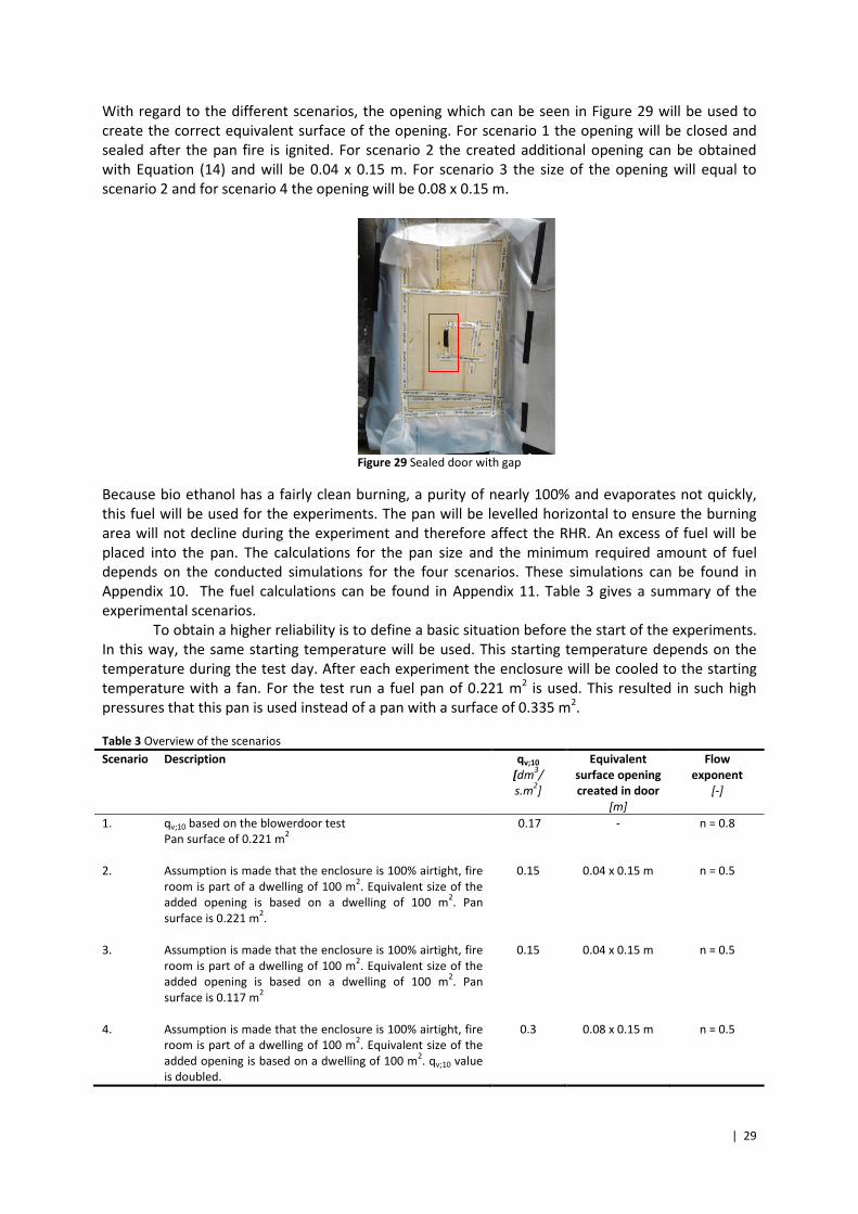
| 29
With regard to the different scenarios, the opening which can be seen in Figure 29 will be used to
create the correct equivalent surface of the opening. For scenario 1 the opening will be closed and
sealed after the pan fire is ignited. For scenario 2 the created additional opening can be obtained
with Equation (14) and will be 0.04 x 0.15 m. For scenario 3 the size of the opening will equal to
scenario 2 and for scenario 4 the opening will be 0.08 x 0.15 m.
Figure 29 Sealed door with gap
Because bio ethanol has a fairly clean burning, a purity of nearly 100% and evaporates not quickly,
this fuel will be used for the experiments. The pan will be levelled horizontal to ensure the burning
area will not decline during the experiment and therefore affect the RHR. An excess of fuel will be
placed into the pan. The calculations for the pan size and the minimum required amount of fuel
depends on the conducted simulations for the four scenarios. These simulations can be found in
Appendix 10. The fuel calculations can be found in Appendix 11. Table 3 gives a summary of the
experimental scenarios.
To obtain a higher reliability is to define a basic situation before the start of the experiments.
In this way, the same starting temperature will be used. This starting temperature depends on the
temperature during the test day. After each experiment the enclosure will be cooled to the starting
temperature with a fan. For the test run a fuel pan of 0.221 m2 is used. This resulted in such high
pressures that this pan is used instead of a pan with a surface of 0.335 m2.
Table 3 Overview of the scenarios
Scenario Description qv;10
[dm3/
s.m2]
Equivalent
surface opening
created in door
[m]
Flow
exponent
[-]
1. qv;10 based on the blowerdoor test
Pan surface of 0.221 m2
0.17 - n = 0.8
2. Assumption is made that the enclosure is 100% airtight, fire
room is part of a dwelling of 100 m2. Equivalent size of the
added opening is based on a dwelling of 100 m2. Pan
surface is 0.221 m2.
0.15 0.04 x 0.15 m n = 0.5
3. Assumption is made that the enclosure is 100% airtight, fire
room is part of a dwelling of 100 m2. Equivalent size of the
added opening is based on a dwelling of 100 m2. Pan
surface is 0.117 m2
0.15 0.04 x 0.15 m n = 0.5
4. Assumption is made that the enclosure is 100% airtight, fire
room is part of a dwelling of 100 m2. Equivalent size of the
added opening is based on a dwelling of 100 m2. qv;10 value
is doubled.
0.3 0.08 x 0.15 m n = 0.5
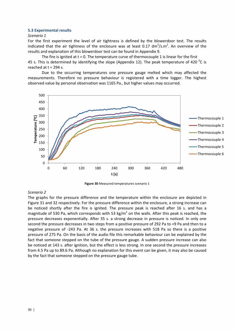
30 |
5.3 Experimental results
Scenario 1
For the first experiment the level of air tightness is defined by the blowerdoor test. The results
indicated that the air tightness of the enclosure was at least 0.17 dm3/s.m
2. An overview of the
results and explanation of this blowerdoor test can be found in Appendix 9.
The fire is ignited at t = 0. The temperature curve of thermocouple 1 is linear for the first
45 s. This is determined by identifying the slope (Appendix 12). The peak temperature of 420 0C is
reached at t = 294 s.
Due to the occurring temperatures one pressure gauge melted which may affected the
measurements. Therefore no pressure behaviour is registered with a time logger. The highest
observed value by personal observation was 1165 Pa., but higher values may occurred.
Figure 30 Measured temperatures scenario 1
Scenario 2
The graphs for the pressure difference and the temperature within the enclosure are depicted in
Figure 31 and 32 respectively. For the pressure difference within the enclosure, a strong increase can
be noticed shortly after the fire is ignited. The pressure peak is reached after 16 s. and has a
magnitude of 530 Pa, which corresponds with 53 kg/m2 on the walls. After this peak is reached, the
pressure decreases exponentially. After 35 s. a strong decrease in pressure is noticed. In only one
second the pressure decreases in two steps from a positive pressure of 292 Pa to +9 Pa and then to a
negative pressure of -243 Pa. At 36 s. the pressure increases with 518 Pa so there is a positive
pressure of 275 Pa. On the basis of the audio file this remarkable behaviour can be explained by the
fact that someone stepped on the tube of the pressure gauge. A sudden pressure increase can also
be noticed at 143 s. after ignition, but the effect is less strong. In one second the pressure increases
from 4.5 Pa up to 89.6 Pa. Although no explanation for this event can be given, it may also be caused
by the fact that someone stepped on the pressure gauge tube.
0
50
100
150
200
250
300
350
400
450
500
0 60 120 180 240 300 360 420 480
Te
mp
era
ture
[0C
]
t [s]
Thermocouple 1
Thermocouple 2
Thermocouple 3
Thermocouple 4
Thermocouple 5
Thermocouple 6
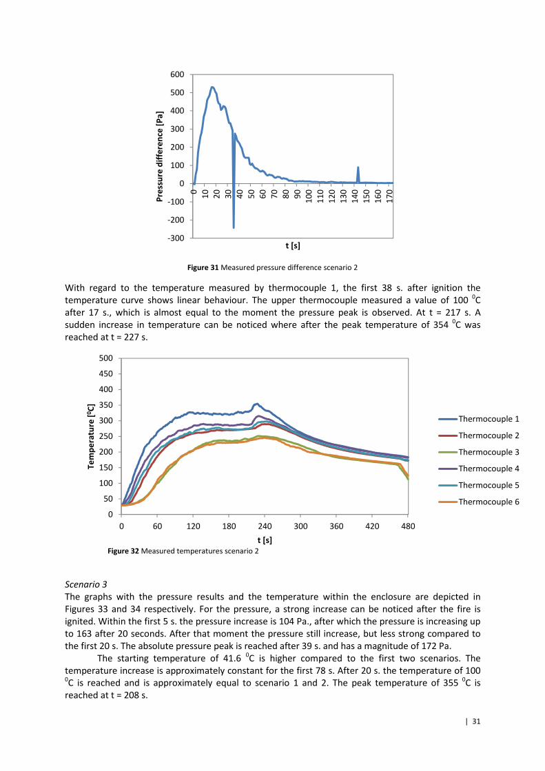
| 31
Figure 31 Measured pressure difference scenario 2
With regard to the temperature measured by thermocouple 1, the first 38 s. after ignition the
temperature curve shows linear behaviour. The upper thermocouple measured a value of 100 0C
after 17 s., which is almost equal to the moment the pressure peak is observed. At t = 217 s. A
sudden increase in temperature can be noticed where after the peak temperature of 354 0C was
reached at t = 227 s.
Scenario 3
The graphs with the pressure results and the temperature within the enclosure are depicted in
Figures 33 and 34 respectively. For the pressure, a strong increase can be noticed after the fire is
ignited. Within the first 5 s. the pressure increase is 104 Pa., after which the pressure is increasing up
to 163 after 20 seconds. After that moment the pressure still increase, but less strong compared to
the first 20 s. The absolute pressure peak is reached after 39 s. and has a magnitude of 172 Pa.
The starting temperature of 41.6 0C is higher compared to the first two scenarios. The
temperature increase is approximately constant for the first 78 s. After 20 s. the temperature of 100 0C is reached and is approximately equal to scenario 1 and 2. The peak temperature of 355
0C is
reached at t = 208 s.
-300
-200
-100
0
100
200
300
400
500
600
0
10
20
30
40
50
60
70
80
90
10
0
11
0
12
0
13
0
14
0
15
0
16
0
17
0
Pre
ssu
re d
iffe
ren
ce [
Pa
]
t [s]
0
50
100
150
200
250
300
350
400
450
500
0 60 120 180 240 300 360 420 480
Te
mp
era
ture
[0C
]
t [s]
Thermocouple 1
Thermocouple 2
Thermocouple 3
Thermocouple 4
Thermocouple 5
Thermocouple 6
Figure 32 Measured temperatures scenario 2
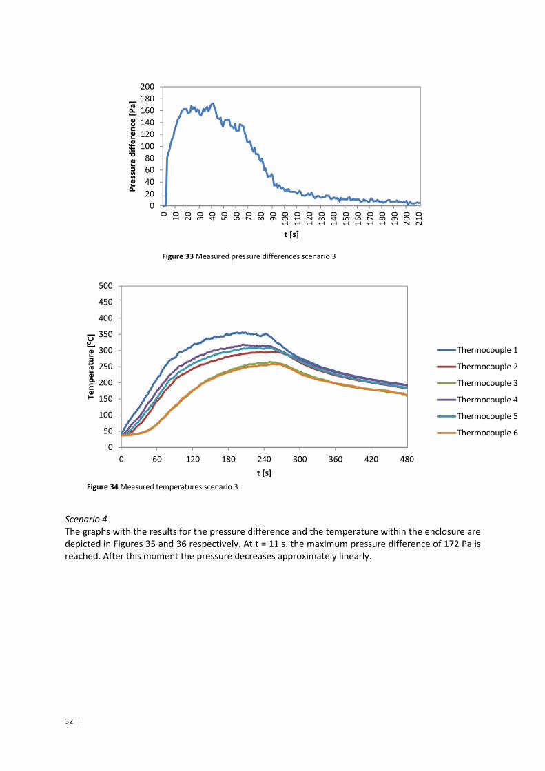
32 |
Figure 33 Measured pressure differences scenario 3
Scenario 4
The graphs with the results for the pressure difference and the temperature within the enclosure are
depicted in Figures 35 and 36 respectively. At t = 11 s. the maximum pressure difference of 172 Pa is
reached. After this moment the pressure decreases approximately linearly.
0
20
40
60
80
100
120
140
160
180
200
0
10
20
30
40
50
60
70
80
90
10
0
11
0
12
0
13
0
14
0
15
0
16
0
17
0
18
0
19
0
20
0
21
0
Pre
ssu
re d
iffe
ren
ce [
Pa
]
t [s]
0
50
100
150
200
250
300
350
400
450
500
0 60 120 180 240 300 360 420 480
Te
mp
era
ture
[0C
]
t [s]
Thermocouple 1
Thermocouple 2
Thermocouple 3
Thermocouple 4
Thermocouple 5
Thermocouple 6
Figure 34 Measured temperatures scenario 3
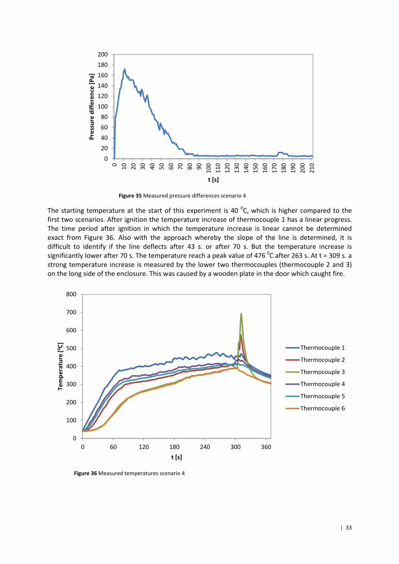
| 33
Figure 35 Measured pressure differences scenario 4
The starting temperature at the start of this experiment is 40 0C, which is higher compared to the
first two scenarios. After ignition the temperature increase of thermocouple 1 has a linear progress.
The time period after ignition in which the temperature increase is linear cannot be determined
exact from Figure 36. Also with the approach whereby the slope of the line is determined, it is
difficult to identify if the line deflects after 43 s. or after 70 s. But the temperature increase is
significantly lower after 70 s. The temperature reach a peak value of 476 0C after 263 s. At t = 309 s. a
strong temperature increase is measured by the lower two thermocouples (thermocouple 2 and 3)
on the long side of the enclosure. This was caused by a wooden plate in the door which caught fire.
Figure 36 Measured temperatures scenario 4
0
20
40
60
80
100
120
140
160
180
200
0
10
20
30
40
50
60
70
80
90
10
0
11
0
12
0
13
0
14
0
15
0
16
0
17
0
18
0
19
0
20
0
21
0
Pre
ssu
re d
iffe
ren
ce [
Pa
]
t [s]
0
100
200
300
400
500
600
700
800
0 60 120 180 240 300 360
Te
mp
era
ture
[0C
]
t [s]
Thermocouple 1
Thermocouple 2
Thermocouple 3
Thermocouple 4
Thermocouple 5
Thermocouple 6
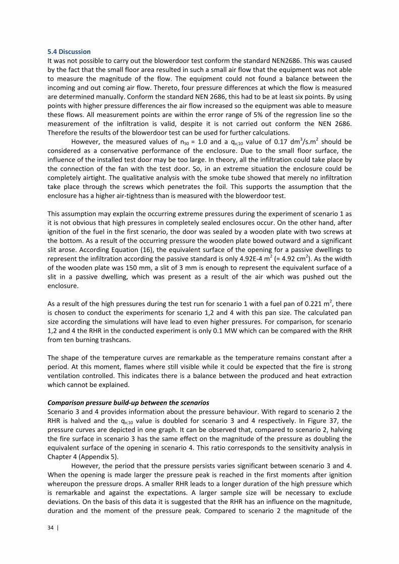
34 |
5.4 Discussion
It was not possible to carry out the blowerdoor test conform the standard NEN2686. This was caused
by the fact that the small floor area resulted in such a small air flow that the equipment was not able
to measure the magnitude of the flow. The equipment could not found a balance between the
incoming and out coming air flow. Thereto, four pressure differences at which the flow is measured
are determined manually. Conform the standard NEN 2686, this had to be at least six points. By using
points with higher pressure differences the air flow increased so the equipment was able to measure
these flows. All measurement points are within the error range of 5% of the regression line so the
measurement of the infiltration is valid, despite it is not carried out conform the NEN 2686.
Therefore the results of the blowerdoor test can be used for further calculations.
However, the measured values of n50 = 1.0 and a qv;10 value of 0.17 dm3/s.m
2 should be
considered as a conservative performance of the enclosure. Due to the small floor surface, the
influence of the installed test door may be too large. In theory, all the infiltration could take place by
the connection of the fan with the test door. So, in an extreme situation the enclosure could be
completely airtight. The qualitative analysis with the smoke tube showed that merely no infiltration
take place through the screws which penetrates the foil. This supports the assumption that the
enclosure has a higher air-tightness than is measured with the blowerdoor test.
This assumption may explain the occurring extreme pressures during the experiment of scenario 1 as
it is not obvious that high pressures in completely sealed enclosures occur. On the other hand, after
ignition of the fuel in the first scenario, the door was sealed by a wooden plate with two screws at
the bottom. As a result of the occurring pressure the wooden plate bowed outward and a significant
slit arose. According Equation (16), the equivalent surface of the opening for a passive dwellings to
represent the infiltration according the passive standard is only 4.92E-4 m2 (= 4.92 cm
2). As the width
of the wooden plate was 150 mm, a slit of 3 mm is enough to represent the equivalent surface of a
slit in a passive dwelling, which was present as a result of the air which was pushed out the
enclosure.
As a result of the high pressures during the test run for scenario 1 with a fuel pan of 0.221 m2, there
is chosen to conduct the experiments for scenario 1,2 and 4 with this pan size. The calculated pan
size according the simulations will have lead to even higher pressures. For comparison, for scenario
1,2 and 4 the RHR in the conducted experiment is only 0.1 MW which can be compared with the RHR
from ten burning trashcans.
The shape of the temperature curves are remarkable as the temperature remains constant after a
period. At this moment, flames where still visible while it could be expected that the fire is strong
ventilation controlled. This indicates there is a balance between the produced and heat extraction
which cannot be explained.
Comparison pressure build-up between the scenarios
Scenario 3 and 4 provides information about the pressure behaviour. With regard to scenario 2 the
RHR is halved and the qv;10 value is doubled for scenario 3 and 4 respectively. In Figure 37, the
pressure curves are depicted in one graph. It can be observed that, compared to scenario 2, halving
the fire surface in scenario 3 has the same effect on the magnitude of the pressure as doubling the
equivalent surface of the opening in scenario 4. This ratio corresponds to the sensitivity analysis in
Chapter 4 (Appendix 5).
However, the period that the pressure persists varies significant between scenario 3 and 4.
When the opening is made larger the pressure peak is reached in the first moments after ignition
whereupon the pressure drops. A smaller RHR leads to a longer duration of the high pressure which
is remarkable and against the expectations. A larger sample size will be necessary to exclude
deviations. On the basis of this data it is suggested that the RHR has an influence on the magnitude,
duration and the moment of the pressure peak. Compared to scenario 2 the magnitude of the
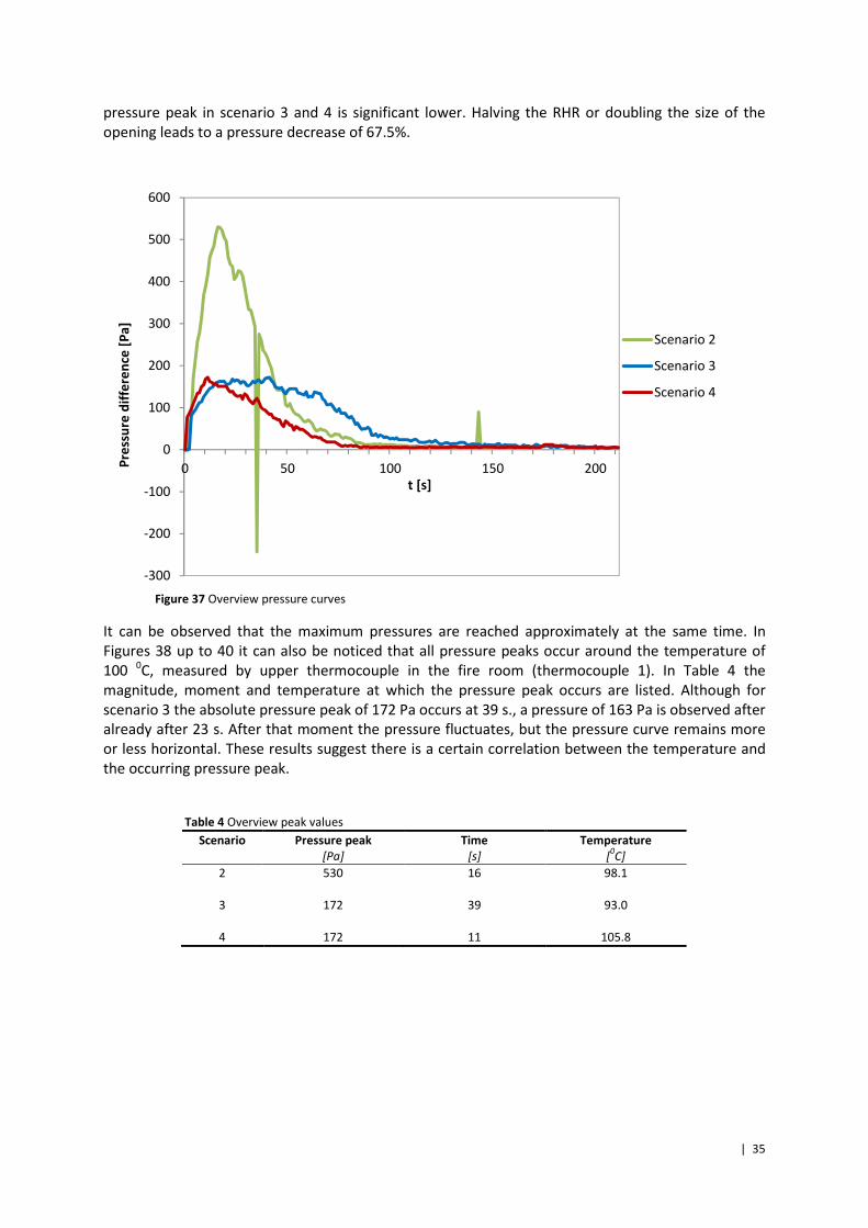
| 35
pressure peak in scenario 3 and 4 is significant lower. Halving the RHR or doubling the size of the
opening leads to a pressure decrease of 67.5%.
Figure 37 Overview pressure curves
It can be observed that the maximum pressures are reached approximately at the same time. In
Figures 38 up to 40 it can also be noticed that all pressure peaks occur around the temperature of
100 0C, measured by upper thermocouple in the fire room (thermocouple 1). In Table 4 the
magnitude, moment and temperature at which the pressure peak occurs are listed. Although for
scenario 3 the absolute pressure peak of 172 Pa occurs at 39 s., a pressure of 163 Pa is observed after
already after 23 s. After that moment the pressure fluctuates, but the pressure curve remains more
or less horizontal. These results suggest there is a certain correlation between the temperature and
the occurring pressure peak.
Table 4 Overview peak values
Scenario Pressure peak
[Pa]
Time
[s]
Temperature
[0C]
2
530 16 98.1
3
172 39 93.0
4 172 11 105.8
-300
-200
-100
0
100
200
300
400
500
600
0 50 100 150 200
Scenario 2
Scenario 3
Scenario 4
Pre
ssu
re d
iffe
ren
ce [
Pa
]
t [s]
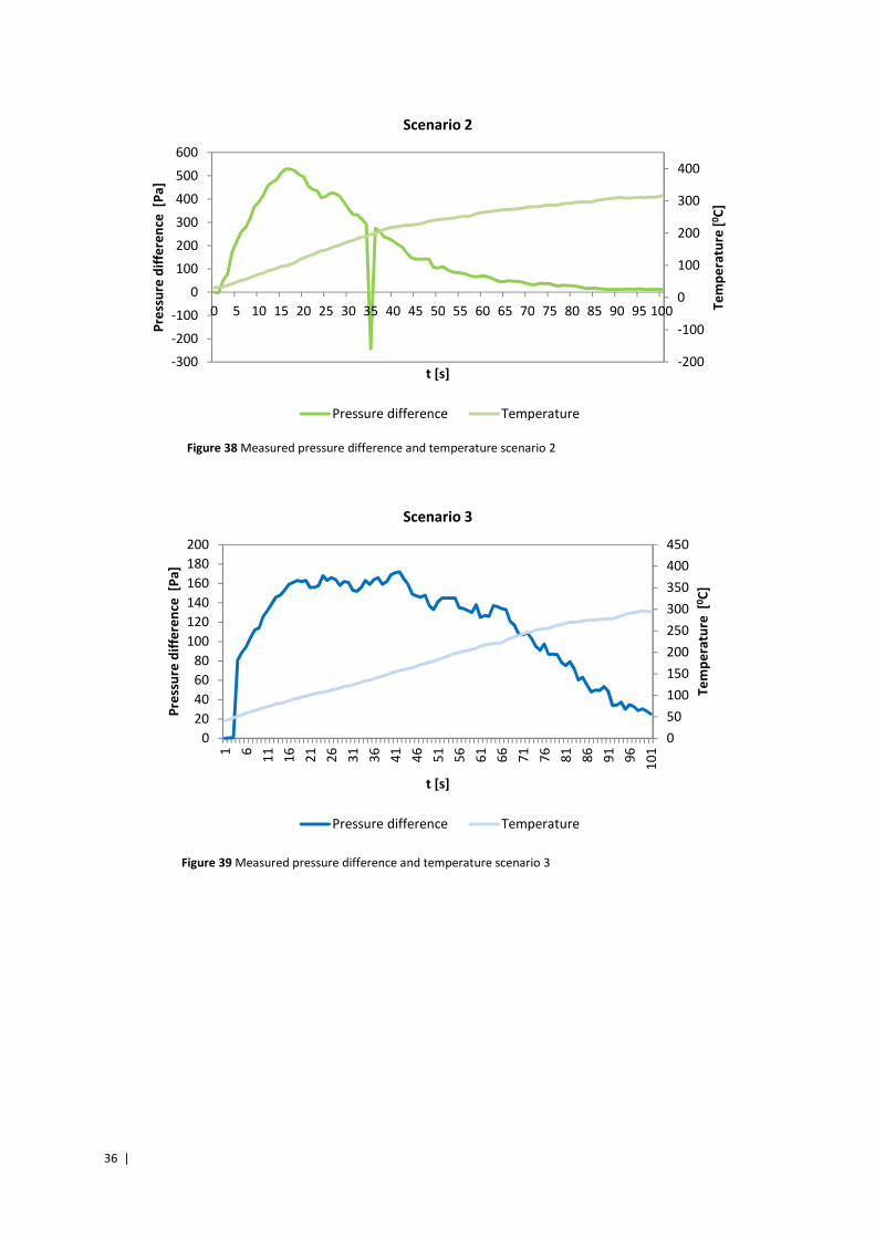
36 |
-200
-100
0
100
200
300
400
-300
-200
-100
0
100
200
300
400
500
600
0 5 10 15 20 25 30 35 40 45 50 55 60 65 70 75 80 85 90 95 100 Te
mp
era
ture
[0C
]
Pre
ssu
re d
iffe
ren
ce [
Pa
]
t [s]
Scenario 2
Pressure difference Temperature
0
50
100
150
200
250
300
350
400
450
0
20
40
60
80
100
120
140
160
180
200
1 6
11
16
21
26
31
36
41
46
51
56
61
66
71
76
81
86
91
96
10
1
Te
mp
era
ture
[0C
]
Pre
ssu
re d
iffe
ren
ce [
Pa
]
t [s]
Scenario 3
Pressure difference Temperature
Figure 38 Measured pressure difference and temperature scenario 2
Figure 39 Measured pressure difference and temperature scenario 3
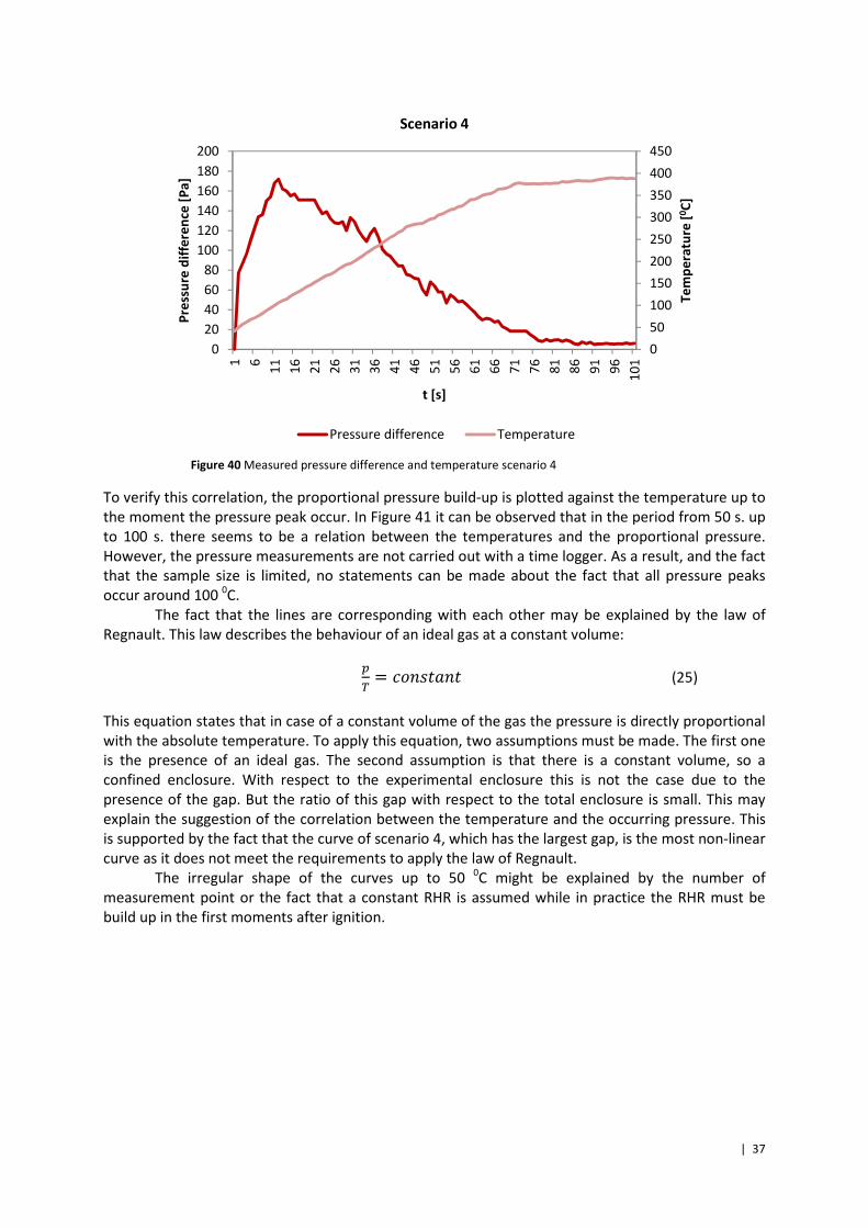
| 37
Figure 40 Measured pressure difference and temperature scenario 4
To verify this correlation, the proportional pressure build-up is plotted against the temperature up to
the moment the pressure peak occur. In Figure 41 it can be observed that in the period from 50 s. up
to 100 s. there seems to be a relation between the temperatures and the proportional pressure.
However, the pressure measurements are not carried out with a time logger. As a result, and the fact
that the sample size is limited, no statements can be made about the fact that all pressure peaks
occur around 100 0C.
The fact that the lines are corresponding with each other may be explained by the law of
Regnault. This law describes the behaviour of an ideal gas at a constant volume:
P, = |}[~�#[� (25)
This equation states that in case of a constant volume of the gas the pressure is directly proportional
with the absolute temperature. To apply this equation, two assumptions must be made. The first one
is the presence of an ideal gas. The second assumption is that there is a constant volume, so a
confined enclosure. With respect to the experimental enclosure this is not the case due to the
presence of the gap. But the ratio of this gap with respect to the total enclosure is small. This may
explain the suggestion of the correlation between the temperature and the occurring pressure. This
is supported by the fact that the curve of scenario 4, which has the largest gap, is the most non-linear
curve as it does not meet the requirements to apply the law of Regnault.
The irregular shape of the curves up to 50 0C might be explained by the number of
measurement point or the fact that a constant RHR is assumed while in practice the RHR must be
build up in the first moments after ignition.
0
50
100
150
200
250
300
350
400
450
0
20
40
60
80
100
120
140
160
180
200
1 6
11
16
21
26
31
36
41
46
51
56
61
66
71
76
81
86
91
96
10
1
Te
mp
era
ture
[0C
]
Pre
ssu
re d
iffe
ren
ce [
Pa
]
t [s]
Scenario 4
Pressure difference Temperature
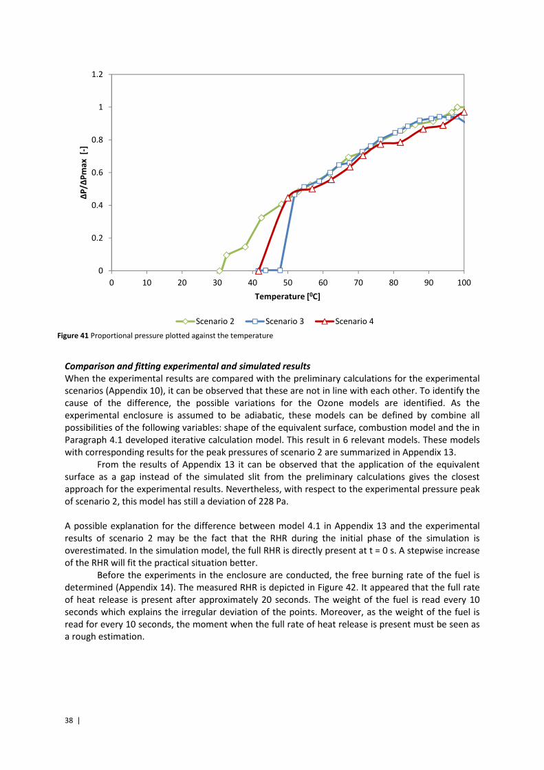
38 |
Comparison and fitting experimental and simulated results
When the experimental results are compared with the preliminary calculations for the experimental
scenarios (Appendix 10), it can be observed that these are not in line with each other. To identify the
cause of the difference, the possible variations for the Ozone models are identified. As the
experimental enclosure is assumed to be adiabatic, these models can be defined by combine all
possibilities of the following variables: shape of the equivalent surface, combustion model and the in
Paragraph 4.1 developed iterative calculation model. This result in 6 relevant models. These models
with corresponding results for the peak pressures of scenario 2 are summarized in Appendix 13.
From the results of Appendix 13 it can be observed that the application of the equivalent
surface as a gap instead of the simulated slit from the preliminary calculations gives the closest
approach for the experimental results. Nevertheless, with respect to the experimental pressure peak
of scenario 2, this model has still a deviation of 228 Pa.
A possible explanation for the difference between model 4.1 in Appendix 13 and the experimental
results of scenario 2 may be the fact that the RHR during the initial phase of the simulation is
overestimated. In the simulation model, the full RHR is directly present at t = 0 s. A stepwise increase
of the RHR will fit the practical situation better.
Before the experiments in the enclosure are conducted, the free burning rate of the fuel is
determined (Appendix 14). The measured RHR is depicted in Figure 42. It appeared that the full rate
of heat release is present after approximately 20 seconds. The weight of the fuel is read every 10
seconds which explains the irregular deviation of the points. Moreover, as the weight of the fuel is
read for every 10 seconds, the moment when the full rate of heat release is present must be seen as
a rough estimation.
0
0.2
0.4
0.6
0.8
1
1.2
0 10 20 30 40 50 60 70 80 90 100
ΔP
/ΔP
ma
x
[-]
Temperature [0C]
Scenario 2 Scenario 3 Scenario 4
Figure 41 Proportional pressure plotted against the temperature
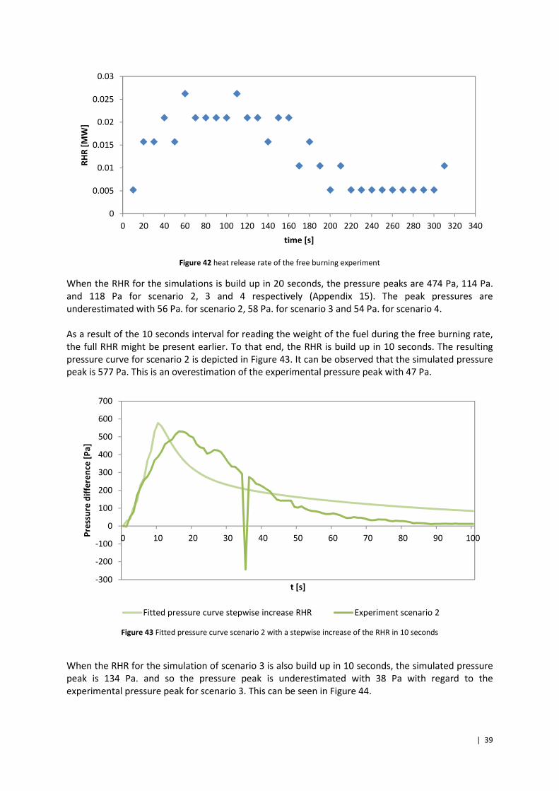
| 39
Figure 42 heat release rate of the free burning experiment
When the RHR for the simulations is build up in 20 seconds, the pressure peaks are 474 Pa, 114 Pa.
and 118 Pa for scenario 2, 3 and 4 respectively (Appendix 15). The peak pressures are
underestimated with 56 Pa. for scenario 2, 58 Pa. for scenario 3 and 54 Pa. for scenario 4.
As a result of the 10 seconds interval for reading the weight of the fuel during the free burning rate,
the full RHR might be present earlier. To that end, the RHR is build up in 10 seconds. The resulting
pressure curve for scenario 2 is depicted in Figure 43. It can be observed that the simulated pressure
peak is 577 Pa. This is an overestimation of the experimental pressure peak with 47 Pa.
Figure 43 Fitted pressure curve scenario 2 with a stepwise increase of the RHR in 10 seconds
When the RHR for the simulation of scenario 3 is also build up in 10 seconds, the simulated pressure
peak is 134 Pa. and so the pressure peak is underestimated with 38 Pa with regard to the
experimental pressure peak for scenario 3. This can be seen in Figure 44.
0
0.005
0.01
0.015
0.02
0.025
0.03
0 20 40 60 80 100 120 140 160 180 200 220 240 260 280 300 320 340
RH
R [
MW
]
time [s]
-300
-200
-100
0
100
200
300
400
500
600
700
0 10 20 30 40 50 60 70 80 90 100Pre
ssu
re d
iffe
ren
ce [
Pa
]
t [s]
Fitted pressure curve stepwise increase RHR Experiment scenario 2
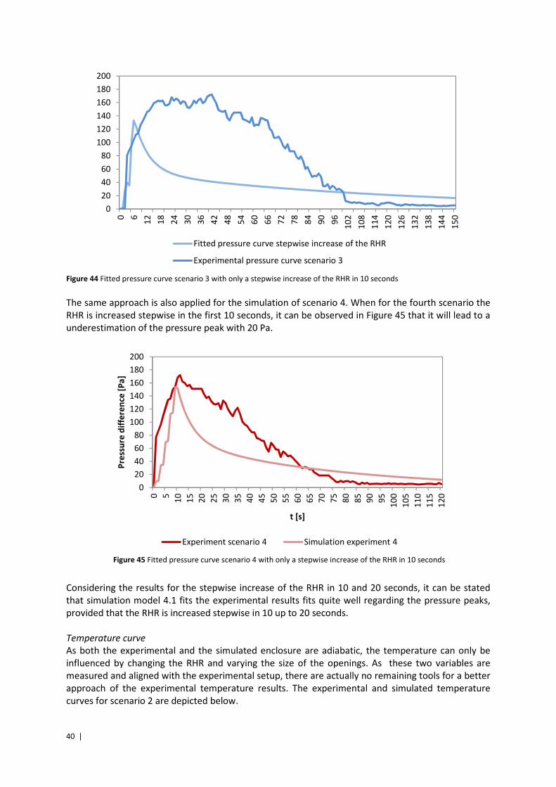
40 |
Figure 44 Fitted pressure curve scenario 3 with only a stepwise increase of the RHR in 10 seconds
The same approach is also applied for the simulation of scenario 4. When for the fourth scenario the
RHR is increased stepwise in the first 10 seconds, it can be observed in Figure 45 that it will lead to a
underestimation of the pressure peak with 20 Pa.
Considering the results for the stepwise increase of the RHR in 10 and 20 seconds, it can be stated
that simulation model 4.1 fits the experimental results fits quite well regarding the pressure peaks,
provided that the RHR is increased stepwise in 10 up to 20 seconds.
Temperature curve
As both the experimental and the simulated enclosure are adiabatic, the temperature can only be
influenced by changing the RHR and varying the size of the openings. As these two variables are
measured and aligned with the experimental setup, there are actually no remaining tools for a better
approach of the experimental temperature results. The experimental and simulated temperature
curves for scenario 2 are depicted below.
0
20
40
60
80
100
120
140
160
180
200
0 6
12
18
24
30
36
42
48
54
60
66
72
78
84
90
96
10
2
10
8
11
4
12
0
12
6
13
2
13
8
14
4
15
0
Fitted pressure curve stepwise increase of the RHR
Experimental pressure curve scenario 3
0
20
40
60
80
100
120
140
160
180
200
0 5
10
15
20
25
30
35
40
45
50
55
60
65
70
75
80
85
90
95
10
0
10
5
11
0
11
5
12
0
Pre
ssu
re d
iffe
ren
ce [
Pa
]
t [s]
Experiment scenario 4 Simulation experiment 4
Figure 45 Fitted pressure curve scenario 4 with only a stepwise increase of the RHR in 10 seconds
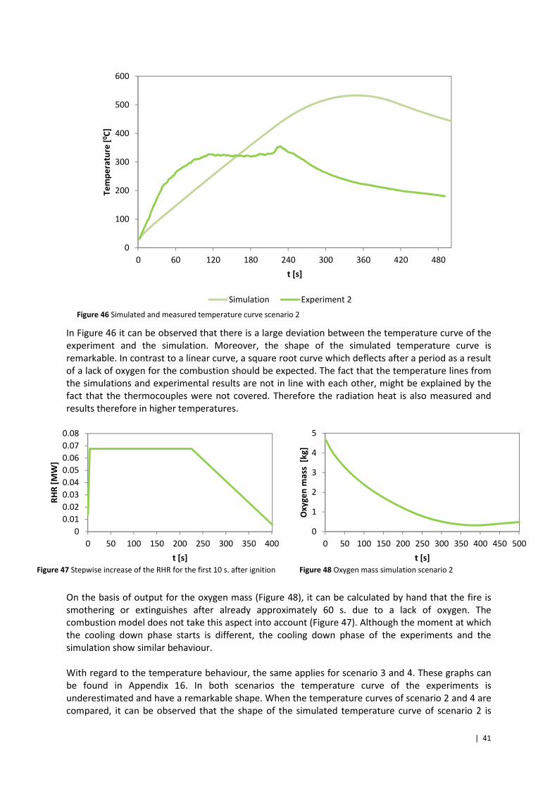
| 41
In Figure 46 it can be observed that there is a large deviation between the temperature curve of the
experiment and the simulation. Moreover, the shape of the simulated temperature curve is
remarkable. In contrast to a linear curve, a square root curve which deflects after a period as a result
of a lack of oxygen for the combustion should be expected. The fact that the temperature lines from
the simulations and experimental results are not in line with each other, might be explained by the
fact that the thermocouples were not covered. Therefore the radiation heat is also measured and
results therefore in higher temperatures.
On the basis of output for the oxygen mass (Figure 48), it can be calculated by hand that the fire is
smothering or extinguishes after already approximately 60 s. due to a lack of oxygen. The
combustion model does not take this aspect into account (Figure 47). Although the moment at which
the cooling down phase starts is different, the cooling down phase of the experiments and the
simulation show similar behaviour.
With regard to the temperature behaviour, the same applies for scenario 3 and 4. These graphs can
be found in Appendix 16. In both scenarios the temperature curve of the experiments is
underestimated and have a remarkable shape. When the temperature curves of scenario 2 and 4 are
compared, it can be observed that the shape of the simulated temperature curve of scenario 2 is
0
100
200
300
400
500
600
0 60 120 180 240 300 360 420 480
Te
mp
era
ture
[0C
]
t [s]
Simulation Experiment 2
0
1
2
3
4
5
0 50 100 150 200 250 300 350 400 450 500
Ox
yg
en
ma
ss
[kg
]
t [s]
Figure 46 Simulated and measured temperature curve scenario 2
0
0.01
0.02
0.03
0.04
0.05
0.06
0.07
0.08
0 50 100 150 200 250 300 350 400
RH
R [
MW
]
t [s]
Figure 47 Stepwise increase of the RHR for the first 10 s. after ignition Figure 48 Oxygen mass simulation scenario 2
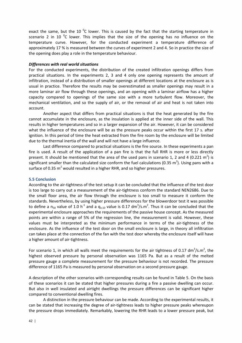
42 |
exact the same, but the 10 0C lower. This is caused by the fact that the starting temperature in
scenario 2 in 10 0C lower. This implies that the size of the opening has no influence on the
temperature curve. However, for the conducted experiment a temperature difference of
approximately 17 % is measured between the curves of experiment 2 and 4. So in practice the size of
the opening does play a role in the temperature behaviour.
Differences with real world situations
For the conducted experiments, the distribution of the created infiltration openings differs from
practical situations. In the experiments 2, 3 and 4 only one opening represents the amount of
infiltration, instead of a distribution of smaller openings at different locations at the enclosure as is
usual in practice. Therefore the results may be overestimated as smaller openings may result in a
more laminar air flow through these openings, and an opening with a laminar airflow has a higher
capacity compared to openings of the same size with a more turbulent flow. Moreover, the
mechanical ventilation, and so the supply of air, or the removal of air and heat is not taken into
account.
Another aspect that differs from practical situations is that the heat generated by the fire
cannot accumulate in the enclosure, as the insulation is applied at the inner side of the wall. This
results in higher temperatures and so in a larger expansion of the air. However, it can be considered
what the influence of the enclosure will be as the pressure peaks occur within the first 17 s. after
ignition. In this period of time the heat extracted from the fire room by the enclosure will be limited
due to the thermal inertia of the wall and will not have a large influence.
Last difference compared to practical situations is the fire source. In these experiments a pan
fire is used. A result of the application of a pan fire is that the full RHR is more or less directly
present. It should be mentioned that the area of the used pans in scenario 1, 2 and 4 (0.221 m2) is
significant smaller than the calculated size conform the fuel calculations (0.35 m2). Using pans with a
surface of 0.35 m2 would resulted in a higher RHR, and so higher pressures.
5.5 Conclusion
According to the air-tightness of the test setup it can be concluded that the influence of the test door
is too large to carry out a measurement of the air-tightness conform the standard NEN2686. Due to
the small floor area, the air flow through the enclosure is too small to measure it conform the
standards. Nevertheless, by using higher pressure differences for the blowerdoor test it was possible
to define a n50 value of 1.0 h-1
and a qv;10 value is 0.17 dm3/s.m
2. Thus it can be concluded that the
experimental enclosure approaches the requirements of the passive house concept. As the measured
points are within a range of 5% of the regression line, the measurement is valid. However, these
values must be interpreted as the minimum performance in terms of the air-tightness of the
enclosure. As the influence of the test door on the small enclosure is large, in theory all infiltration
can takes place at the connection of the fan with the test door whereby the enclosure itself will have
a higher amount of air-tightness.
For scenario 1, in which all walls meet the requirements for the air tightness of 0.17 dm3/s.m
2, the
highest observed pressure by personal observation was 1165 Pa. But as a result of the melted
pressure gauge a complete measurement for the pressure behaviour is not recorded. The pressure
difference of 1165 Pa is measured by personal observation on a second pressure gauge.
A description of the other scenarios with corresponding results can be found in Table 5. On the basis
of these scenarios it can be stated that higher pressures during a fire a passive dwelling can occur.
But also in well insulated and airtight dwellings the pressure differences can be significant higher
compared to conventional dwelling fires.
A distinction in the pressure behaviour can be made. According to the experimental results, it
can be stated that increasing the degree of air-tightness leads to higher pressure peaks whereupon
the pressure drops immediately. Remarkably, lowering the RHR leads to a lower pressure peak, but
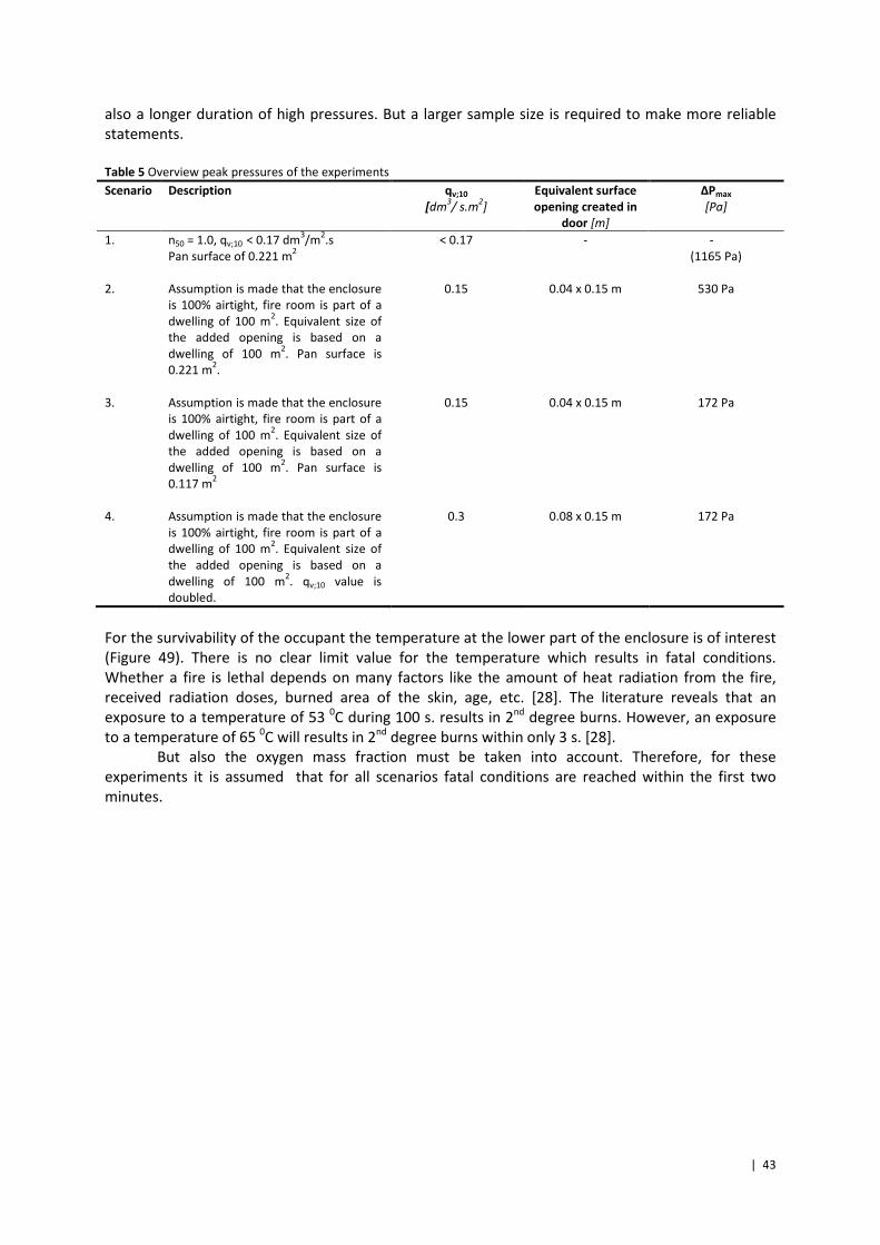
| 43
also a longer duration of high pressures. But a larger sample size is required to make more reliable
statements.
Table 5 Overview peak pressures of the experiments
Scenario Description qv;10
[dm3/ s.m
2]
Equivalent surface
opening created in
door [m]
ΔPmax
[Pa]
1. n50 = 1.0, qv;10 < 0.17 dm3/m
2.s
Pan surface of 0.221 m2
< 0.17 - -
(1165 Pa)
2. Assumption is made that the enclosure
is 100% airtight, fire room is part of a
dwelling of 100 m2. Equivalent size of
the added opening is based on a
dwelling of 100 m2. Pan surface is
0.221 m2.
0.15 0.04 x 0.15 m 530 Pa
3. Assumption is made that the enclosure
is 100% airtight, fire room is part of a
dwelling of 100 m2. Equivalent size of
the added opening is based on a
dwelling of 100 m2. Pan surface is
0.117 m2
0.15 0.04 x 0.15 m 172 Pa
4. Assumption is made that the enclosure
is 100% airtight, fire room is part of a
dwelling of 100 m2. Equivalent size of
the added opening is based on a
dwelling of 100 m2. qv;10 value is
doubled.
0.3 0.08 x 0.15 m 172 Pa
For the survivability of the occupant the temperature at the lower part of the enclosure is of interest
(Figure 49). There is no clear limit value for the temperature which results in fatal conditions.
Whether a fire is lethal depends on many factors like the amount of heat radiation from the fire,
received radiation doses, burned area of the skin, age, etc. [28]. The literature reveals that an
exposure to a temperature of 53 0C during 100 s. results in 2
nd degree burns. However, an exposure
to a temperature of 65 0C will results in 2
nd degree burns within only 3 s. [28].
But also the oxygen mass fraction must be taken into account. Therefore, for these
experiments it is assumed that for all scenarios fatal conditions are reached within the first two
minutes.
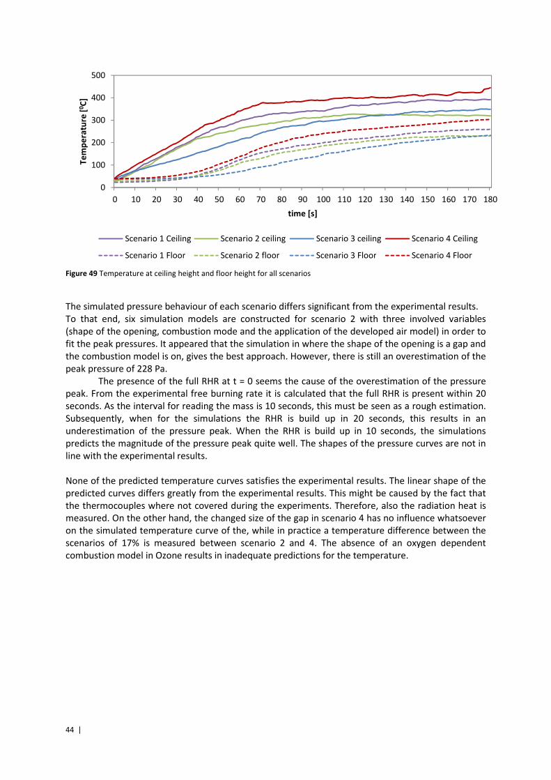
44 |
Figure 49 Temperature at ceiling height and floor height for all scenarios
The simulated pressure behaviour of each scenario differs significant from the experimental results.
To that end, six simulation models are constructed for scenario 2 with three involved variables
(shape of the opening, combustion mode and the application of the developed air model) in order to
fit the peak pressures. It appeared that the simulation in where the shape of the opening is a gap and
the combustion model is on, gives the best approach. However, there is still an overestimation of the
peak pressure of 228 Pa.
The presence of the full RHR at t = 0 seems the cause of the overestimation of the pressure
peak. From the experimental free burning rate it is calculated that the full RHR is present within 20
seconds. As the interval for reading the mass is 10 seconds, this must be seen as a rough estimation.
Subsequently, when for the simulations the RHR is build up in 20 seconds, this results in an
underestimation of the pressure peak. When the RHR is build up in 10 seconds, the simulations
predicts the magnitude of the pressure peak quite well. The shapes of the pressure curves are not in
line with the experimental results.
None of the predicted temperature curves satisfies the experimental results. The linear shape of the
predicted curves differs greatly from the experimental results. This might be caused by the fact that
the thermocouples where not covered during the experiments. Therefore, also the radiation heat is
measured. On the other hand, the changed size of the gap in scenario 4 has no influence whatsoever
on the simulated temperature curve of the, while in practice a temperature difference between the
scenarios of 17% is measured between scenario 2 and 4. The absence of an oxygen dependent
combustion model in Ozone results in inadequate predictions for the temperature.
0
100
200
300
400
500
0 10 20 30 40 50 60 70 80 90 100 110 120 130 140 150 160 170 180
Te
mp
era
ture
[0C
]
time [s]
Scenario 1 Ceiling Scenario 2 ceiling Scenario 3 ceiling Scenario 4 Ceiling
Scenario 1 Floor Scenario 2 floor Scenario 3 Floor Scenario 4 Floor
| 45
6. Discussion
This research is focussed on the influence of the building skin on the fire behaviour in well insulated
and airtight dwellings, and in particular the pressure behaviour with regard to the safety of the
occupant and fire service. Until now it was assumed that window pane breakage as a result of
internal material stresses was normative for the safety.
In order to give an answer, the relevant variables are selected by a literature study. The simulation
programme Ozone is used to give an insight in the fire and pressure behaviour. In order to create a
robust answer a probabilistic scenario analysis is carried out, and at a higher level, a regression
analysis over the two most important variables is conducted. The results are validated by conducting
real scale fire experiments.
With regard to the internal validation, it is sought to base the input parameters on standards
and prescriptive rules like the Dutch building code, NEN2687, NEN-EN 1991-1-2/NB and the
Eurocode EN 1990, annex B. With regard to the internal validation it is chosen to use the passive
building concept as a starting point, as the characteristics are quantified.
In practice, the results will be strongly influenced by random factors. One can think of windows that
are opened, window pane breakage and the initial fire object.
With regard to the simulations and the sensitiveness analysis it must be mentioned that
these results only applies for dwellings of 100 m2. A different dwelling size may lead to different
results. To find a solution for the shortcoming of Ozone to apply a flow exponent ≠ 0.5, other
programmes like CONTAM are considered. However, in these programmes it is not possible to apply
a RHR curve. Finally, this research focuses at the fire behaviour at room level. Although there is
looked at the influence of the remaining area of the dwelling on the fire room, a closer look at this
interaction may result in different outcomes.
For each scenario only one experiment is conducted. As fire source a pan fire is used. As a
result, the full RHR is directly present. Although the pan size is adjusted on the simulated pressure
peak as a result of the curve from the EN 1991-1-2, and is even reduced on the basis of the pressure
results after the test run for scenario 1, this may affect the pressure behaviour. Due to the clean
combustion of the fuel, no smoke is produced. Moreover, the enclosure is expected to be adiabatic
and the infiltration is translated into an equivalent opening. Due to the small floor area only a
maximum value for the infiltration could be measured with the blowerdoor test.
The research objectives have been achieved in that an insight is given in the fire and pressure
behaviour in well insulated and airtight and passive dwellings. Although there are some limitations,
statements can be made. The fire behaviour and in particular the pressure behaviour has been
observed in practice at full scale and recommendations for suppressive actions and safety for the
occupant can be made.
The results of this research show that more knowledge is required about current practical
situations and the ability to simulate fires in passive dwellings must be increased. The simplifications
in the experimental rig resulted in a reduction of time and money. Now it has been shown that high
pressures can occur, more extensive experiments can be conducted to overcome the limitations of
this research.

46 |
| 47
7. Conclusion
Ability to simulate the fire and pressure behaviour
The simulation of the pressure behaviour in well insulated and airtight dwellings in Ozone is
inadequate as a result of a fixed value of n = 0.5 for the flow exponent and the calculation for the
magnitude of the air flow at a fixed pressure difference of 10 Pa. To determine the air flow as a result
of the infiltration, which is translated into a slit over the entire height of the compartment, an
additional iterative calculation tool is developed. This iterative calculation tool adapts the size of the
slit on the occurring higher pressures. However, this results in an underestimation of the pressure
peaks.
The simulation of the temperature behaviour in Ozone is inadequate as a result of the
absence of an oxygen dependent combustion model.
Fire and pressure behaviour in well insulated and airtight dwellings
The pressure increase in dwelling fires is determined by 6 variables, which are the Rate of Heat
Release, amount of infiltration (qv;10 value), volume of the room, mechanical ventilation, type of
enclosure and the Rc- value of the enclosure. The qv;10 value, the size of the compartment and the
RHR have descending the largest influence on the pressure build-up during fire.
For the simulated enclosure with the arbitrary dimensions of 4.0 x 5.0 x 2.6 m. (w x l x h), which can
represent a small living room or large bedroom, a strong ventilation controlled fire with a RHR of
0.65 MW and a pressure peak of 64 Pa can be expected. As a result of the stochastic deviation of the
variables and a lack of knowledge about practical situations it can be concluded that, with the
required degree of certainty according the building code, the pressure peak of 64 Pa will be
exceeded.
From the experiments it appeared that high pressures in the order of hundreds of Pa can occur
during fires in both well insulated and passive dwellings. However, the extent to which these
pressures really occur and so determines the fire scenario will depend on the building characteristics,
heat release rate and coincidental factors. During the experiments, the temperature within the
compartment increases rapidly. Within 75 seconds the temperature at floor level exceeds 100 0C for
all conducted scenarios.
Safety for the occupant and fire service
The pressure increase will play a role in the safety of the occupant as the pressure peaks occurred
within the first 23 seconds after ignition. It may prevent the occupant to escape the dwelling as it will
be difficult or even impossible to open inward turning doors. In combination with the strong
temperature increase this will lead to fatal circumstances within a minute.
Given the expected fire behaviour in well insulated and airtight dwellings, the fire service will
not be able to carry out an offensive insight attack in order to rescue the occupant. If openings are
created below the neutral plane the RHR will increase rapidly or a smoke gas explosion could take
place. If openings are created above the neutral plane a backdraft could take place.
In theory, the fire service can expect a strong ventilation controlled fire which may have already been
gone out as a result of a lack of oxygen. This results in a potential dangerous situation as it cannot be
excluded that the fire is still smothering. In that case a sudden supply of oxygen can lead to a very
rapid increase of the RHR, backdraft or smoke gas explosion.
In practice the fire and pressure behaviour will be determined by coincidental factors
like opened door and windows. Another possibility is that the pressure increase may lead to the
occurrence of unplanned ventilation openings as a pressure increase of several hundreds of Pa in
combination with the occurring temperatures may have an influence on the structural integrity of

48 |
window panes. Therefore, the fire service can expect a wide range of scenarios. As the pressure
peaks occurred at the first moments after ignition during the fire growth stage, it will have no direct
influence on the safety of the fire service.
| 49
8. Recommendations
As a result of the findings in this research the following recommendations can be made:
• It is expected that the application of a flow exponent of n ≠ 0.5 and oxygen dependent
combustion model in Ozone will improve the ability to predict the fire and pressure
behaviour in passive dwellings. This is supported by the fact that Ozone gives somewhat
reasonable results for the peak pressures in the simulations of the conducted experiments
when a gap is modelled and the RHR is increased stepwise. It can be recommended to
integrate these possibilities in Ozone.
• No general recommendations for the strategy of the fire service in well insulated and airtight
dwellings can be given, as the fire service can face a wide range of scenarios as a result of
coincidental factors. However, a distinction in possible scenarios can be made. On the basis
of the individual scenarios and the quadrant model [30] it is possible to make
recommendations for the strategy of the fire service. The following scenarios are
distinguished:
� Local smouldering fire
� Local flaming fire
� Compartment on fire with external flames
In case of a local smouldering fire without casualties it can be recommended to do nothing
and wait until the fire spontaneously go out as a result of a lack of oxygen. In case of
casualties, no inside attack can be carried out as the scenario is expected to be strong
ventilation controlled and the fire source cannot be localized. Therefore it will be too
dangerous to carry out an offensive inside attack.
In case of a local flaming fire without casualties, an attack from the inside is not possible as
additional openings may lead to a backdraft, smoke gas explosion or a very quick increase of
the RHR. A defensive strategy from the outside can be applied. An offensive attack from the
outside is possible to reduce damage. But any additional oxygen supply will result in greater
damage and expose the fire fighters to danger.
In case of casualties, in theory the offensive outside attack might be followed by an
offensive inside attack, provided that it is certain that there are no heat sources anymore and
the hot gases are cooled. However, given the time that has been elapsed since the ignition of
the fire, it is expected that the survivability for the occupant is nil.
In case of a compartment fire with external flaming, an offensive attack from the outside can
be applied. A careful consideration must made to apply an attack from the inside as the fire
can still be ventilation controlled, even when window panes are fallen out. An additional
oxygen supply can therefore result in a quick increase of the RHR.
• For well insulated and airtight dwellings it can be recommended to apply a CO or smoke
detection system in every room to establish detection in a very early state of the fire.
However, with the moment of the pressure increase and the rapid temperature increase, this
may not be sufficient to escape the dwelling on time in many situations. A rapid intervention
to eliminate the cause of the hazards is required. This can be done by applying dwelling
sprinklers.
50 |
• Dwellings should be designed such that at least for one escape route doors are turning open
into the flee direction. Then it will be possible for the occupant to open doors. Therefore it
can be recommended to flee through the back door since back doors always open to the
outside. In absence of a back door it can be recommended to apply a pressure relaxation
device in the façade which opens at a pressure increase of 50 Pa. This can be compared with
a positive pressure system in stairwells.
• For further research, it can be recommended to conduct more experiments on a larger scale
with multiple rooms in order to obtain a higher reliability for the blowerdoor test, and to give
an insight in the interaction between the fire room and remaining area of the dwelling. This
provides also an insight in the survivability in adjacent rooms and so the necessity for an
offensive attack from the inside in case of a local flaming fire.
For a better approximation of practical situations, a more accurate distribution of
infiltration openings instead of an equivalent surface is recommended. Moreover, the
application of solid fuels will result in a fire curve which fits practical situations better. This
provides also the possibility to take the smoke layer height into account with regard to the
safety of the occupant, and gives an insight in the ability of the occurrence of a smoke gas
explosion.
• The sensitivity study identified that more practical data must be generated about the values
for the amount of infiltration (qv;10) and Rate of Heat Release in practical situations. This
makes it possible to make more robust statements about the pressure behaviour in practical
situations.

| 51
52 |
References
[1] Centraal Bureau voor de Statistiek, 2014. Brandweerstatistiek 2013. Available at:
< http://www.cbs.nl/nl-NL/menu/themas/veiligheidrecht/publicaties/publicaties/archief/2014/2014-
brandweerstatistiek-2013-pub.htm>
[Accessed at 23 September 2014]
[2] Ministerie van Binnenlandse Zaken en koninkrijksrelaties, 2012. Koepelconvenant
Energiebesparing Gebouwde Omgeving. Available at:
<http://www.rijksoverheid.nl/documenten-en-
publicaties/convenanten/2012/06/28/koepelconvenant-energiebesparing-gebouwde-
omgeving.html>
[Accessed 18 March 2014].
[3] Nieman, H., 2012. Luchtdicht bouwen; De theorie en het waarom. Available at:
<http://www.nieman.nl/wp-content/uploads/2012/05/Luchtdicht-bouwen-Harry-Nieman.pdf>
[Accessed at 14 August 2014].
[4] FOD Binnenlandse Zaken, 2010. Brand in een passiefhuis = inferno?; Brandveiligheid in
passiefhuizen. Available at:
<http://besafe.ibz.be/publications/passief-huis.pdf>
[Accessed at 8 November 2013].
[5] Underwriters Laboratories, 2012. Analysis of Changing Residential Fire Dynamics and its
Implications on Firefighter Operational Timeframes. Available at:
http://www.ul.com/global/documents/newscience/whitepapers/firesafety/FS_Analysis%20of%20Ch
anging%20Residential%20Fire%20Dynamics%20and%20Its%20Implications_10-12.pdf
[Accessed at 18 November 2013].
[6] Underwriters Laboratories, 2010. Analysis of One and Two-Story Single Family Home Fire
Dynamics and the Impact of Firefighter Horizontal Ventilation. Available at:
<http://www.ul.com/global/documents/newscience/whitepapers/firesafety/FS_Analysis%20of%20O
ne%20and%20Two-Story%20Single%20Family%20Home%20Fire%20Dynamics_10-12.pdf. >
[Accessed at 18 November 2013].
[7] Herpen, Van R.A.P., 2011. Passiefhuisconcept: brandveilig? Adviesbureau Nieman. Available at:
<http://www.infopuntveiligheid.nl/Infopuntdocumenten/3.%20Ruud%20van%20Herpen.pdf.>
[Accessed at 23 November 2013].
[8] Debrouwere, B., 2012. A study on initial fire behaviour in low-energy houses. Gent University,
Department of Flow, Heat and Combustion (Floheacom). Available at:
<http://www.vvba.nl/downloads/nominaties/A%20study%20on%20initial%20fire%20behaviour%20i
n%20low%20energy%20houses.pdf>
[Accessed at 23 November 2013].
[9] Instituut Fysieke Veiligheid, 2013. Fatale woningbranden 2008 t/m 2012: een vergelijking.
Available at:
http://www.nifv.nl/web/show/file/id=253360/filename=Vergelijking_fatale_woningbranden_2008-
2012.pdf/page=189250.
[Accessed at 20 November 2013].
| 53
[10] Hasofer, A.M., Thomas, I., 2006. Analysis of fatalities and injuries in building fire statistics. Fire
Safety Journal; 41, 2-14.
[Accessed at 15 November 2013].
[11] Bengtsson, L.G., 2001. Enclosure fires. s.l.: Swedish Rescue Services Agency.
[12] Svensson, S., 2005. Fire Ventilation. s.l.: Swedish Rescue Services Agency.
[13] Herpen, R.A.P., 2013. Meerzone luchtstroommodellen. Available at:
< http://www.nvbv.org/index.php?option=com_edocman&view=document&id=312&Itemid=271 >
[Accessed at 2 May 2014]
[14] Mierlo, van R. and Tromp, A., 2013. Fire Safety Engineering- handboek voor de bouw. Delft:
Eburon.
[15] Brink, Van den V., 2015. Fire Safety and Suppression in Modern Residential Buildings. An
experimental research to the Influence of the Building Skin on the Fire Behaviour in Well Insulated
Dwellings and its Consequences for the Safety of the Occupant and Strategy of the Fire Service –
Literature study.
[16] Prétrel, H., Saux, Le W., Audouin, L., 2012. Pressure variations induced by a pool fire in a well-
confined and force-ventilated compartment. Fire Safety Journal; 52, 11-24.
[17] Bonte, F., Noterman, N., Merci, B., 2013. Computer simulations to study interaction between
burning rates and pressure variations in confined enclosure fires. Fire Safety Journal; 62,125-143.
[18] Suard, S., Hostikka, S., Baccou, J., 2013. Sensitivity analysis of fire models using a fractional
factorial design. Fire Safety Journal; 62, 115-124.
[19] Chow, W.K., Zou, G.W., 2009. Numerical simulation of pressure changes in closed chamber fires.
Building and Environment; 44, 1261-1275.
[20] PassivHaus Institut, 2013. Zertifiziertes Passivhaus; Zertifizierungskriterien für Passivhäuser mit
Wohnnutzung. Available at:
< http://www.passiv.de/downloads/03_zertifizierungskriterien_wohngebaeude_de.pdf>
[Accessed at 2 September 2014]
[21] SBRCURnet, 2012. Passiefhuisconcept voor woningbouw. SBR. Available at:
< http://www.sbrcurnet.nl/producten/infobladen/passiefhuisconcept-voor-woningbouw>
[Accessed at 9 August 2014].
[22] SBRCURnet, 2013. Luchtdicht bouwen; Theorie-ontwerp-praktijk. SBR. Available at:
< http://www.sbrcurnet.nl/producten/kennisarchief/luchtdicht-bouwen/bijlage-1-
voorbeeldberekeningen >
[Accessed at 24 April 2014]
[23] Linssen, J.P.A., 2011. Brand in huis; Overleven of overlijden. Available at:
http://www.infopuntveiligheid.nl/Infopuntdocumenten/20111001%20Linssen%20FSE%20Brand%20i
n%20huis_overleven%20of%20overlijden.pdf
[Accessed at 21 November 2013]

54 |
[24] Baum, R., Floyd, J., Hostikka, S., McGrattan, K., Rehm, R., 2007. Fire Dynamics Simulator (Version
5) Technical Reference Guide. NIST Special Publication 1018-5.
[25] Lundin, J., 1999. Model Uncertainty in Fire Safety Engineering. Department of Fire Safety
Engineering, Lund University. Report 1020. Available at:
< https://lup.lub.lu.se/luur/download?func=downloadFile&recordOId=525794&fileOId=642195>
[Accessed at 22 November 2013]
[26] Herpen, R.A.P., 2014. Fysisch brandmodel; Afstemming risiconiveau aan publiekrechtelijke
regelgeving constructieve veiligheid. Available at:
<http://www.nieman.nl/wp-content/uploads/2012/01/Fysisch-brandmodel-Afstemming-
risiconiveau-aan-publiekrechtelijke-regelgeving-constructieve-veiligheid_Ruud-van-
Herpen_2009.pdf>
[Accessed at 23 December 2014]
[27] Herpen, Van R.A.P.,2007. Fysisch brandmodel. Achtergronden; Normalisatie fysisch brandmodel
- Statistische en probabilistische aspecten. Available at:
< http://nieman.nl/2007/06/fysisch-brandmodel/ >
[Accessed at 23 December 2014]
[28] Ministerie van Binnenlandse Zaken en Koninkrijksrelaties, 2003. Publicatiereeks Gevaarlijke
Stoffen 1. Deel 1A: Effecten van brand op personen. Available at:
< http://content.publicatiereeksgevaarlijkestoffen.nl/documents/PGS1/PGS1-2005-v0.1-deel-1a.pdf>
[Accessed at 21 March 2015]
[29] Hagen, R., 2014. Brandpreventie voor repressief leidinggevenden. Available at:
< http://www.ifv.nl/kennisplein/Paginas/Lectoraat-Brandweerkunde.aspx#tab2 >
[Accessed at 11 February 2015]
In Appendix 11 :
[30] Karlsson, B., Quintiere, J.G., 2000. Enclosure Fire Dynamics. CRC Press LLC, Florida. Available at:
< http://unina.stidue.net/Politecnico%20di%20Milano/Ingegneria%20Strutturale/Corsi/Felicetti%20-
%20Fire%20resistance%20of%20materials%20and%20structures/Books/Enclosure%20fire%20dynam
ics/Contents.pdf>
[Accessed at 23 March 2014]
| 55
Appendices
Appendix 1: Classification air tightness
Appendix 2: Input Ozone Chapter 4 “Computational approach”.
Appendix 3: Alternative approach iterative calculation process
Appendix 4: Uncertainties in simulations
Appendix 5: Parameter study – Results
Appendix 6: Results probabilistic scenario analysis
Appendix 7: Multiple linear regression model
Appendix 8: Calculation insulation covering for experimental enclosure
Appendix 9: Results blowerdoor test
Appendix 10: Simulation experimental scenarios
Appendix 11: Fuel calculation experiments
Appendix 12: Analysis moment of deflection of the temperature curves on the basis of the slope of
the line
Appendix 13: Overview fitted simulation models
Appendix 14: Mass loss rate free burning experiment
Appendix 15: Stepwise increase RHR in 20 s.
Appendix 16: Temperature behaviour scenario 3 and 4
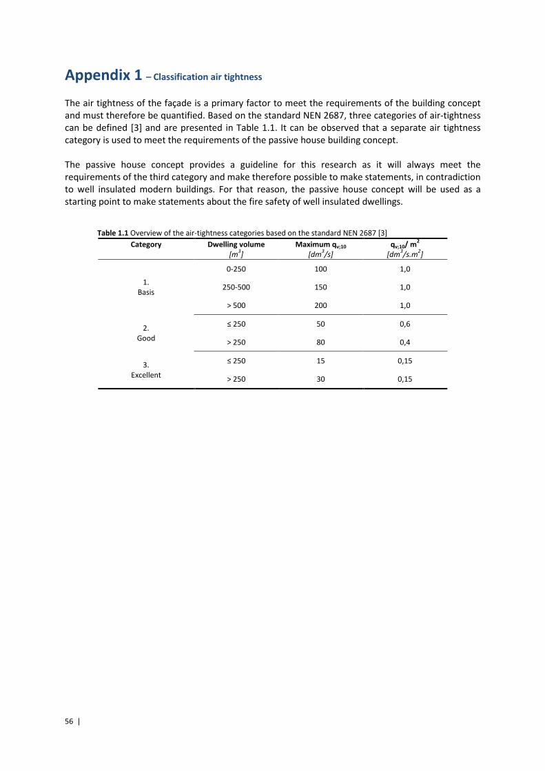
56 |
Appendix 1 – Classification air tightness
The air tightness of the façade is a primary factor to meet the requirements of the building concept
and must therefore be quantified. Based on the standard NEN 2687, three categories of air-tightness
can be defined [3] and are presented in Table 1.1. It can be observed that a separate air tightness
category is used to meet the requirements of the passive house building concept.
The passive house concept provides a guideline for this research as it will always meet the
requirements of the third category and make therefore possible to make statements, in contradiction
to well insulated modern buildings. For that reason, the passive house concept will be used as a
starting point to make statements about the fire safety of well insulated dwellings.
Table 1.1 Overview of the air-tightness categories based on the standard NEN 2687 [3]
Category Dwelling volume
[m3]
Maximum qv;10
[dm3/s]
qv;10/ m2
[dm3/s.m
2]
1.
Basis
0-250 100 1,0
250-500 150 1,0
> 500 200 1,0
2.
Good
≤ 250 50 0,6
> 250 80 0,4
3.
Excellent
≤ 250 15 0,15
> 250 30 0,15
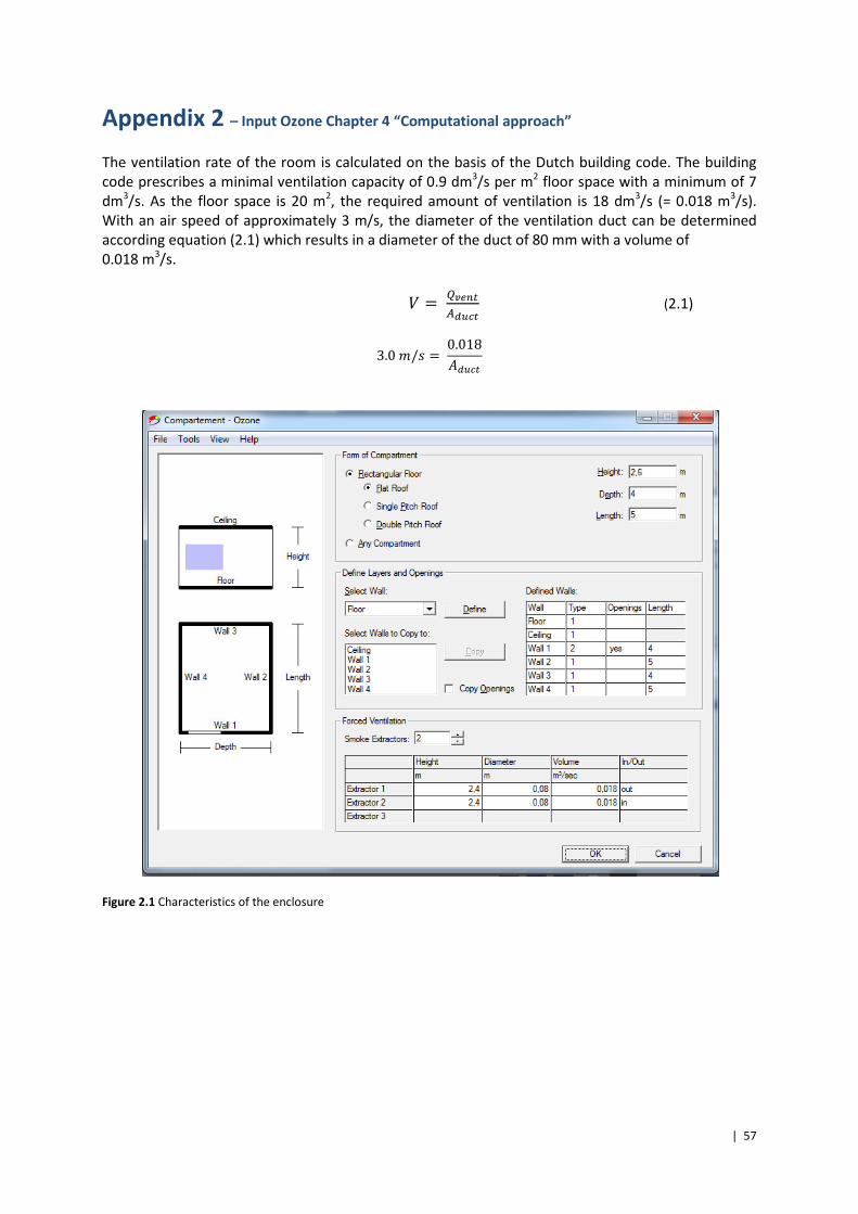
| 57
Appendix 2 – Input Ozone Chapter 4 “Computational approach”
The ventilation rate of the room is calculated on the basis of the Dutch building code. The building
code prescribes a minimal ventilation capacity of 0.9 dm3/s per m
2 floor space with a minimum of 7
dm3/s. As the floor space is 20 m
2, the required amount of ventilation is 18 dm
3/s (= 0.018 m
3/s).
With an air speed of approximately 3 m/s, the diameter of the ventilation duct can be determined
according equation (2.1) which results in a diameter of the duct of 80 mm with a volume of
0.018 m3/s.
A = 69<�W'���W (2.1)
3.0@/~ = 0.018Fw�8]
Figure 2.1 Characteristics of the enclosure
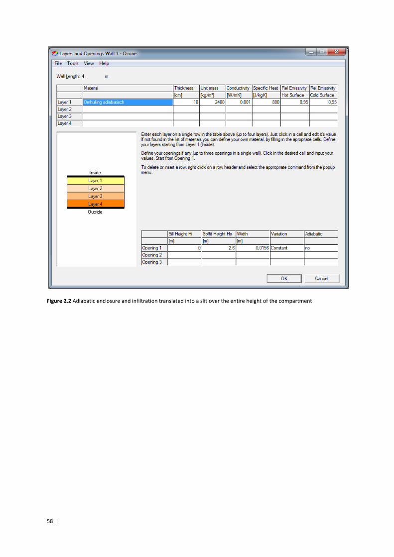
58 |
Figure 2.2 Adiabatic enclosure and infiltration translated into a slit over the entire height of the compartment
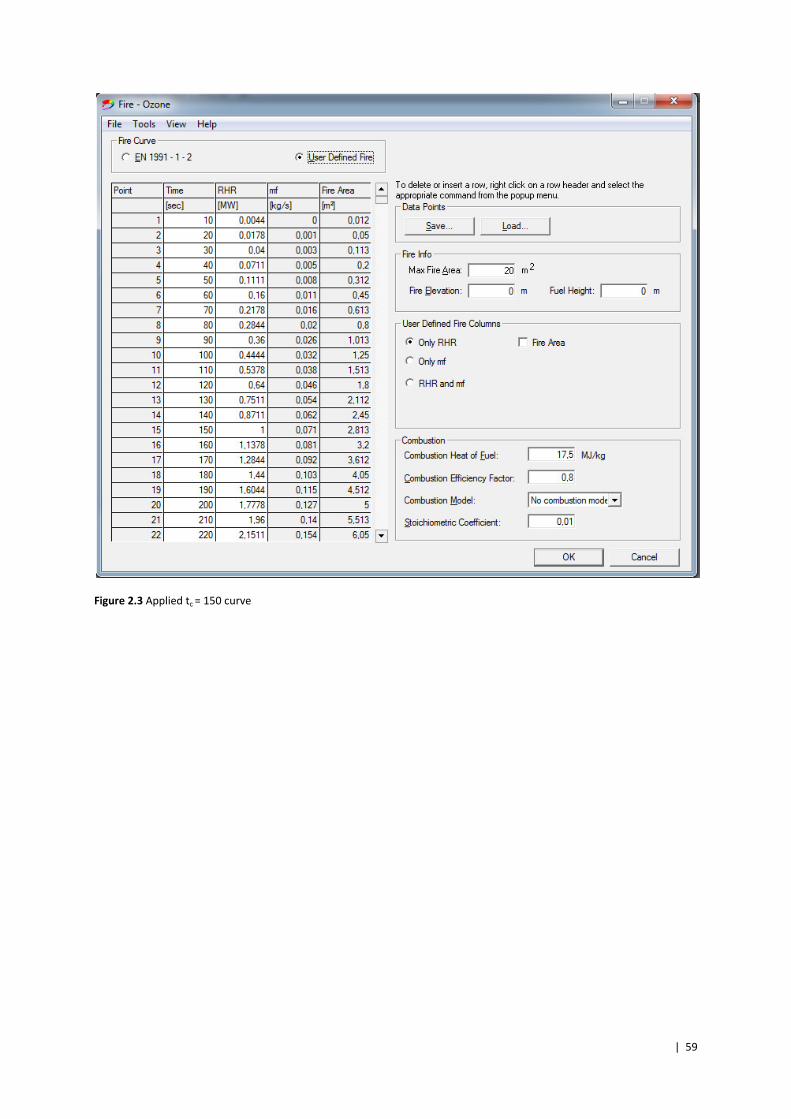
| 59
Figure 2.3 Applied tc = 150 curve
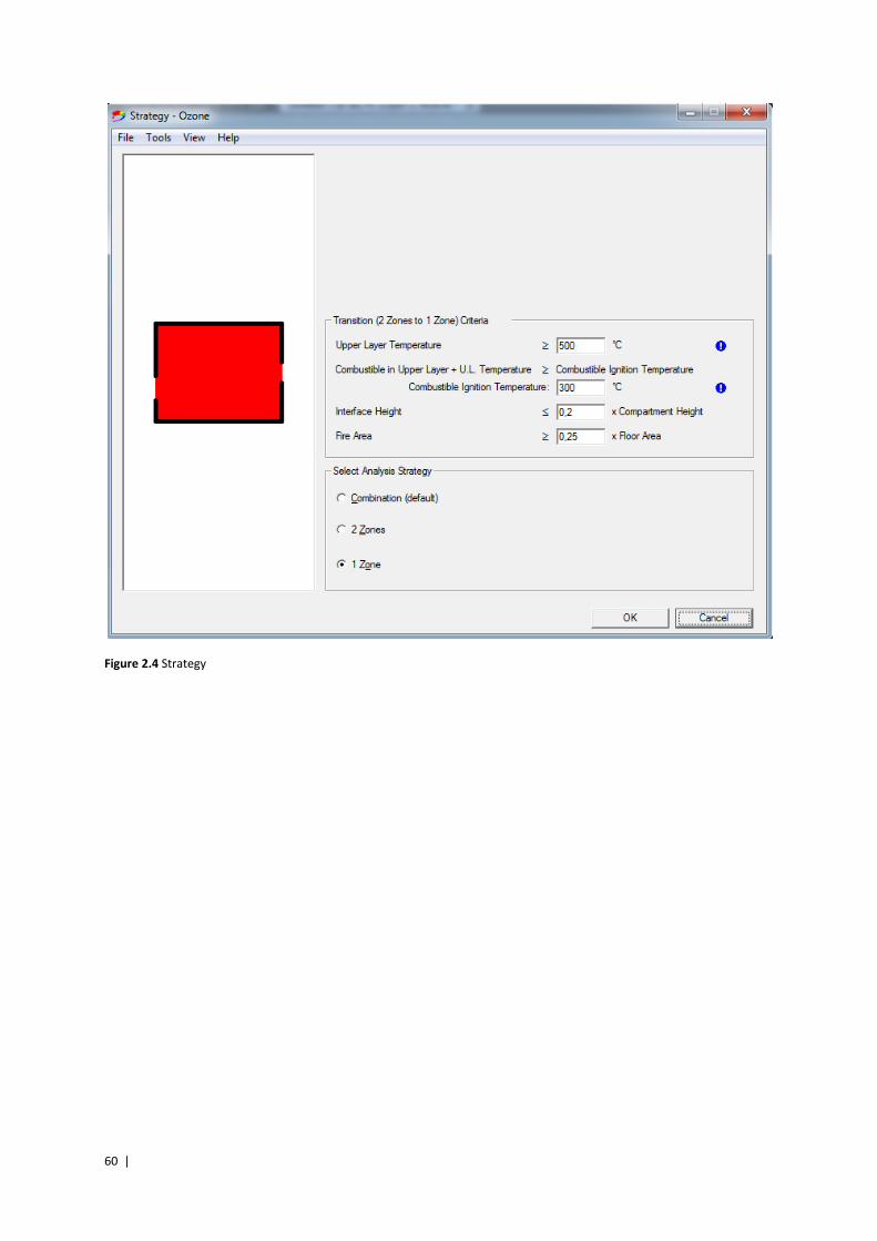
60 |
Figure 2.4 Strategy
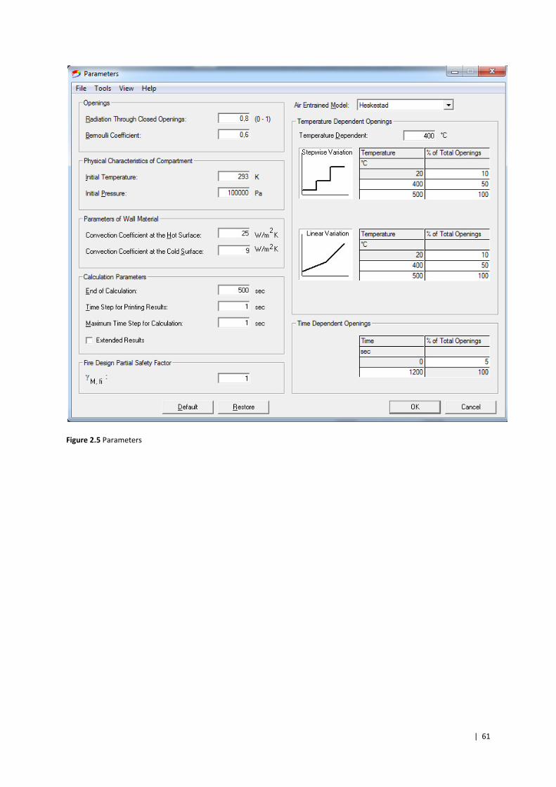
| 61
Figure 2.5 Parameters
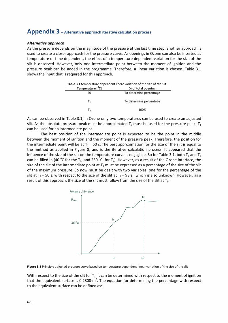
62 |
Appendix 3 – Alternative approach iterative calculation process
Alternative approach
As the pressure depends on the magnitude of the pressure at the last time step, another approach is
used to create a closer approach for the pressure curve. As openings in Ozone can also be inserted as
temperature or time dependent, the effect of a temperature dependent variation for the size of the
slit is observed. However, only one intermediate point between the moment of ignition and the
pressure peak can be added in the programme. Therefore, a linear variation is chosen. Table 3.1
shows the input that is required for this approach.
Table 3.1 temperature dependent linear variation of the size of the slit
Temperature [0C] % of total opening
20
To determine percentage
T1
To determine percentage
T2
100%
As can be observed in Table 3.1, in Ozone only two temperatures can be used to create an adjusted
slit. As the absolute pressure peak must be approximated T2 must be used for the pressure peak. T1
can be used for an intermediate point.
The best position of the intermediate point is expected to be the point in the middle
between the moment of ignition and the moment of the pressure peak. Therefore, the position for
the intermediate point will be at T1 = 50 s. The best approximation for the size of the slit is equal to
the method as applied in Figure 8, and is the iterative calculation process. It appeared that the
influence of the size of the slit on the temperature curve is negligible. So for Table 3.1, both T1 and T2
can be filled in (40 0C for the T1, and 250
0C for T2). However, as a result of the Ozone interface, the
size of the slit of the intermediate point at T1 must be expressed as a percentage of the size of the slit
of the maximum pressure. So now must be dealt with two variables; one for the percentage of the
slit at T1 = 50 s. with respect to the size of the slit at T2 = 93 s., which is also unknown. However, as a
result of this approach, the size of the slit must follow from the size of the slit at T1.
Figure 3.1 Principle adjusted pressure curve based on temperature dependent linear variation of the size of the slit
With respect to the size of the slit for T1, it can be determined with respect to the moment of ignition
that the equivalent surface is 0.2808 m2. The equation for determining the percentage with respect
to the equivalent surface can be defined as:
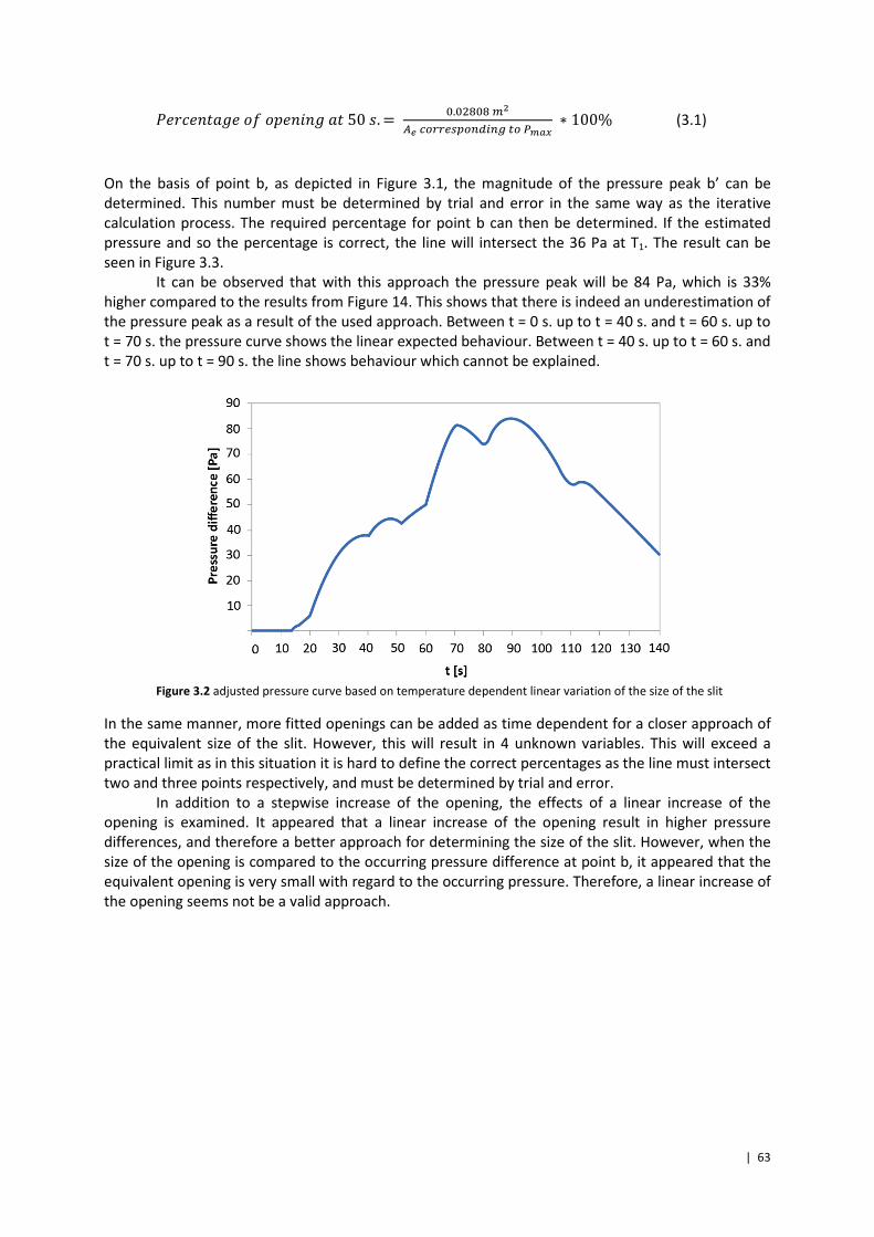
| 63
���|�[�#"�}�}S�[�["#�50~. = I.I�MIMn�'<8tssG�Pt�wU��]t/=*�
∗ 100% (3.1)
On the basis of point b, as depicted in Figure 3.1, the magnitude of the pressure peak b’ can be
determined. This number must be determined by trial and error in the same way as the iterative
calculation process. The required percentage for point b can then be determined. If the estimated
pressure and so the percentage is correct, the line will intersect the 36 Pa at T1. The result can be
seen in Figure 3.3.
It can be observed that with this approach the pressure peak will be 84 Pa, which is 33%
higher compared to the results from Figure 14. This shows that there is indeed an underestimation of
the pressure peak as a result of the used approach. Between t = 0 s. up to t = 40 s. and t = 60 s. up to
t = 70 s. the pressure curve shows the linear expected behaviour. Between t = 40 s. up to t = 60 s. and
t = 70 s. up to t = 90 s. the line shows behaviour which cannot be explained.
Figure 3.2 adjusted pressure curve based on temperature dependent linear variation of the size of the slit
In the same manner, more fitted openings can be added as time dependent for a closer approach of
the equivalent size of the slit. However, this will result in 4 unknown variables. This will exceed a
practical limit as in this situation it is hard to define the correct percentages as the line must intersect
two and three points respectively, and must be determined by trial and error.
In addition to a stepwise increase of the opening, the effects of a linear increase of the
opening is examined. It appeared that a linear increase of the opening result in higher pressure
differences, and therefore a better approach for determining the size of the slit. However, when the
size of the opening is compared to the occurring pressure difference at point b, it appeared that the
equivalent opening is very small with regard to the occurring pressure. Therefore, a linear increase of
the opening seems not be a valid approach.
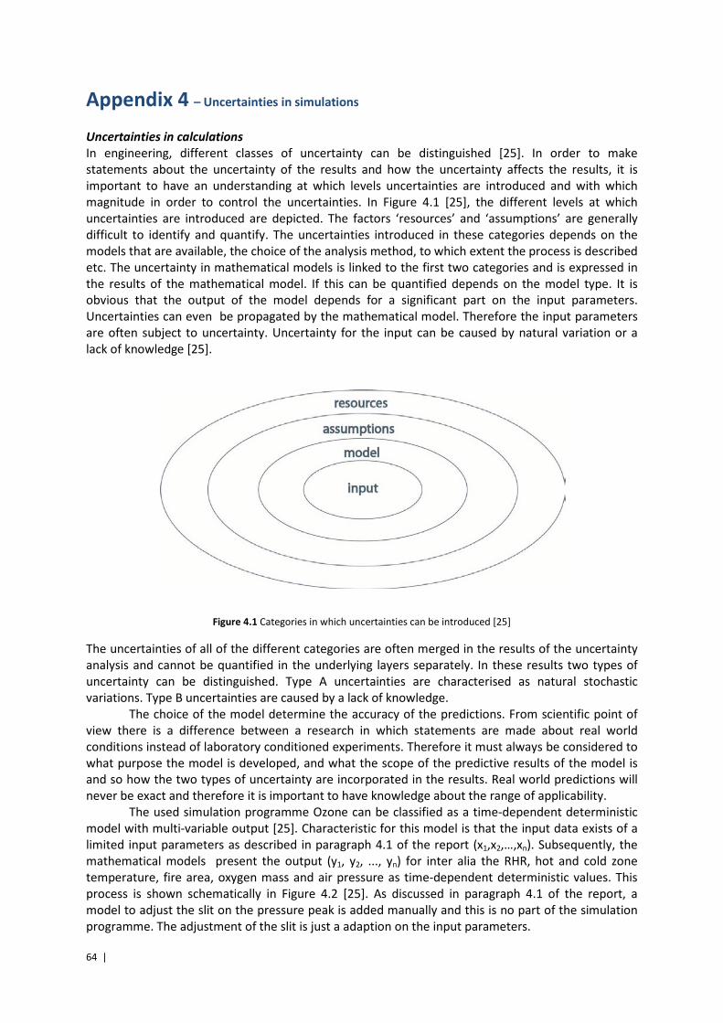
64 |
Appendix 4 – Uncertainties in simulations
Uncertainties in calculations
In engineering, different classes of uncertainty can be distinguished [25]. In order to make
statements about the uncertainty of the results and how the uncertainty affects the results, it is
important to have an understanding at which levels uncertainties are introduced and with which
magnitude in order to control the uncertainties. In Figure 4.1 [25], the different levels at which
uncertainties are introduced are depicted. The factors ‘resources’ and ‘assumptions’ are generally
difficult to identify and quantify. The uncertainties introduced in these categories depends on the
models that are available, the choice of the analysis method, to which extent the process is described
etc. The uncertainty in mathematical models is linked to the first two categories and is expressed in
the results of the mathematical model. If this can be quantified depends on the model type. It is
obvious that the output of the model depends for a significant part on the input parameters.
Uncertainties can even be propagated by the mathematical model. Therefore the input parameters
are often subject to uncertainty. Uncertainty for the input can be caused by natural variation or a
lack of knowledge [25].
Figure 4.1 Categories in which uncertainties can be introduced [25]
The uncertainties of all of the different categories are often merged in the results of the uncertainty
analysis and cannot be quantified in the underlying layers separately. In these results two types of
uncertainty can be distinguished. Type A uncertainties are characterised as natural stochastic
variations. Type B uncertainties are caused by a lack of knowledge.
The choice of the model determine the accuracy of the predictions. From scientific point of
view there is a difference between a research in which statements are made about real world
conditions instead of laboratory conditioned experiments. Therefore it must always be considered to
what purpose the model is developed, and what the scope of the predictive results of the model is
and so how the two types of uncertainty are incorporated in the results. Real world predictions will
never be exact and therefore it is important to have knowledge about the range of applicability.
The used simulation programme Ozone can be classified as a time-dependent deterministic
model with multi-variable output [25]. Characteristic for this model is that the input data exists of a
limited input parameters as described in paragraph 4.1 of the report (x1,x2,…,xn). Subsequently, the
mathematical models present the output (y1, y2, ..., yn) for inter alia the RHR, hot and cold zone
temperature, fire area, oxygen mass and air pressure as time-dependent deterministic values. This
process is shown schematically in Figure 4.2 [25]. As discussed in paragraph 4.1 of the report, a
model to adjust the slit on the pressure peak is added manually and this is no part of the simulation
programme. The adjustment of the slit is just a adaption on the input parameters.

| 65
Figure 4.2 Schematic overview Ozone as time-dependent deterministic model [25]
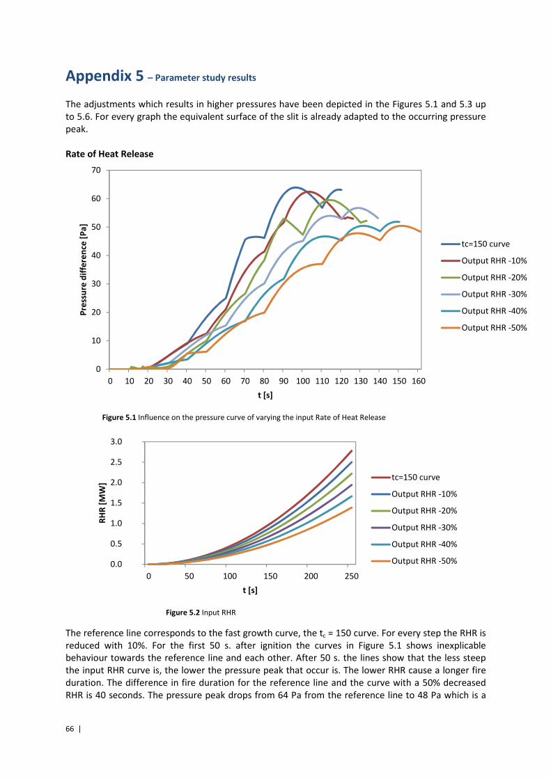
66 |
Appendix 5 – Parameter study results
The adjustments which results in higher pressures have been depicted in the Figures 5.1 and 5.3 up
to 5.6. For every graph the equivalent surface of the slit is already adapted to the occurring pressure
peak.
Rate of Heat Release
Figure 5.1 Influence on the pressure curve of varying the input Rate of Heat Release
Figure 5.2 Input RHR
The reference line corresponds to the fast growth curve, the tc = 150 curve. For every step the RHR is
reduced with 10%. For the first 50 s. after ignition the curves in Figure 5.1 shows inexplicable
behaviour towards the reference line and each other. After 50 s. the lines show that the less steep
the input RHR curve is, the lower the pressure peak that occur is. The lower RHR cause a longer fire
duration. The difference in fire duration for the reference line and the curve with a 50% decreased
RHR is 40 seconds. The pressure peak drops from 64 Pa from the reference line to 48 Pa which is a
0
10
20
30
40
50
60
70
0 10 20 30 40 50 60 70 80 90 100 110 120 130 140 150 160
Pre
ssu
re d
iffe
ren
ce [
Pa
]
t [s]
tc=150 curve
Output RHR -10%
Output RHR -20%
Output RHR -30%
Output RHR -40%
Output RHR -50%
0.0000
0.5000
1.0000
1.5000
2.0000
2.5000
3.0000
0 50 100 150 200 250
RH
R [
MW
]
t [s]
tc=150 curve
Output RHR -10%
Output RHR -20%
Output RHR -30%
Output RHR -40%
Output RHR -50%
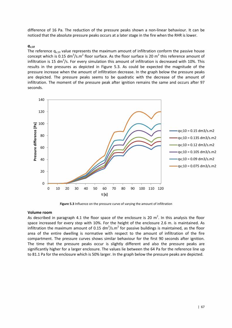
| 67
difference of 16 Pa. The reduction of the pressure peaks shown a non-linear behaviour. It can be
noticed that the absolute pressure peaks occurs at a later stage in the fire when the RHR is lower.
qv;10
The reference qv;10 value represents the maximum amount of infiltration conform the passive house
concept which is 0.15 dm3/s.m
2 floor surface. As the floor surface is 20 m
2 this reference amount of
infiltration is 15 dm3/s. For every simulation this amount of infiltration is decreased with 10%. This
results in the pressures as depicted in Figure 5.3. As could be expected the magnitude of the
pressure increase when the amount of infiltration decrease. In the graph below the pressure peaks
are depicted. The pressure peaks seems to be quadratic with the decrease of the amount of
infiltration. The moment of the pressure peak after ignition remains the same and occurs after 97
seconds.
Figure 5.3 Influence on the pressure curve of varying the amount of infiltration
Volume room
As described in paragraph 4.1 the floor space of the enclosure is 20 m2. In this analysis the floor
space increased for every step with 10%. For the height of the enclosure 2.6 m. is maintained. As
infiltration the maximum amount of 0.15 dm3/s.m
2 for passive buildings is maintained, as the floor
area of the entire dwelling is normative with respect to the amount of infiltration of the fire
compartment. The pressure curves shows similar behaviour for the first 90 seconds after ignition.
The time that the pressure peaks occur is slightly different and also the pressure peaks are
significantly higher for a larger enclosure. The values lie between the 64 Pa for the reference line up
to 81.1 Pa for the enclosure which is 50% larger. In the graph below the pressure peaks are depicted.
0
20
40
60
80
100
120
140
0 10 20 30 40 50 60 70 80 90 100 110 120
Pre
ssu
re d
iffe
ren
ce [
Pa
]
t [s]
qv;10 = 0.15 dm3/s.m2
qv;10 = 0.135 dm3/s.m2
qv;10 = 0.12 dm3/s.m2
qv;10 = 0.105 dm3/s.m2
qv;10 = 0.09 dm3/s.m2
qv;10 = 0.075 dm3/s.m2
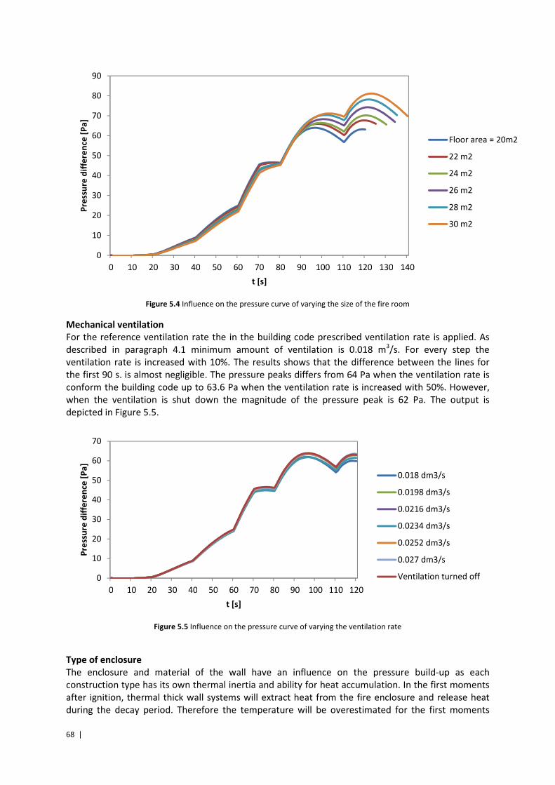
68 |
Figure 5.4 Influence on the pressure curve of varying the size of the fire room
Mechanical ventilation
For the reference ventilation rate the in the building code prescribed ventilation rate is applied. As
described in paragraph 4.1 minimum amount of ventilation is 0.018 m3/s. For every step the
ventilation rate is increased with 10%. The results shows that the difference between the lines for
the first 90 s. is almost negligible. The pressure peaks differs from 64 Pa when the ventilation rate is
conform the building code up to 63.6 Pa when the ventilation rate is increased with 50%. However,
when the ventilation is shut down the magnitude of the pressure peak is 62 Pa. The output is
depicted in Figure 5.5.
Figure 5.5 Influence on the pressure curve of varying the ventilation rate
Type of enclosure
The enclosure and material of the wall have an influence on the pressure build-up as each
construction type has its own thermal inertia and ability for heat accumulation. In the first moments
after ignition, thermal thick wall systems will extract heat from the fire enclosure and release heat
during the decay period. Therefore the temperature will be overestimated for the first moments
0
10
20
30
40
50
60
70
80
90
0 10 20 30 40 50 60 70 80 90 100 110 120 130 140
Pre
ssu
re d
iffe
ren
ce [
Pa
]
t [s]
Floor area = 20m2
22 m2
24 m2
26 m2
28 m2
30 m2
0
10
20
30
40
50
60
70
0 10 20 30 40 50 60 70 80 90 100 110 120
Pre
ssu
re d
iffe
ren
ce [
Pa
]
t [s]
0.018 dm3/s
0.0198 dm3/s
0.0216 dm3/s
0.0234 dm3/s
0.0252 dm3/s
0.027 dm3/s
Ventilation turned off
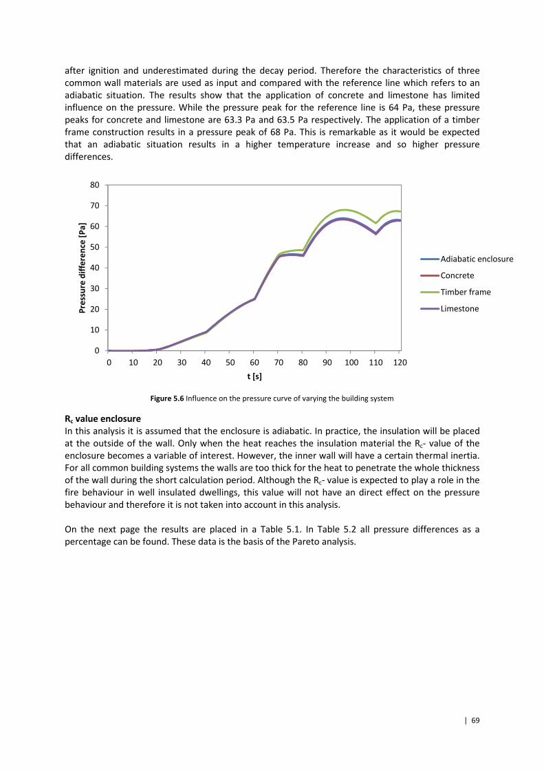
| 69
after ignition and underestimated during the decay period. Therefore the characteristics of three
common wall materials are used as input and compared with the reference line which refers to an
adiabatic situation. The results show that the application of concrete and limestone has limited
influence on the pressure. While the pressure peak for the reference line is 64 Pa, these pressure
peaks for concrete and limestone are 63.3 Pa and 63.5 Pa respectively. The application of a timber
frame construction results in a pressure peak of 68 Pa. This is remarkable as it would be expected
that an adiabatic situation results in a higher temperature increase and so higher pressure
differences.
Figure 5.6 Influence on the pressure curve of varying the building system
Rc value enclosure
In this analysis it is assumed that the enclosure is adiabatic. In practice, the insulation will be placed
at the outside of the wall. Only when the heat reaches the insulation material the Rc- value of the
enclosure becomes a variable of interest. However, the inner wall will have a certain thermal inertia.
For all common building systems the walls are too thick for the heat to penetrate the whole thickness
of the wall during the short calculation period. Although the Rc- value is expected to play a role in the
fire behaviour in well insulated dwellings, this value will not have an direct effect on the pressure
behaviour and therefore it is not taken into account in this analysis.
On the next page the results are placed in a Table 5.1. In Table 5.2 all pressure differences as a
percentage can be found. These data is the basis of the Pareto analysis.
0
10
20
30
40
50
60
70
80
0 10 20 30 40 50 60 70 80 90 100 110 120
Pre
ssu
re d
iffe
ren
ce [
Pa
]
t [s]
Adiabatic enclosure
Concrete
Timber frame
Limestone
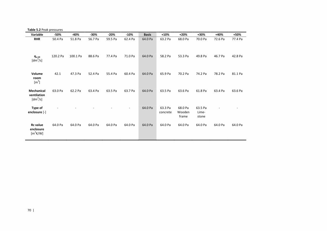
70 |
Table 5.2 Peak pressures
Variable -50% -40% -30% -20% -10% Basis +10% +20% +30% +40% +50%
RHR 50.4 Pa 51.8 Pa 56.7 Pa 59.5 Pa 62.4 Pa 64.0 Pa 63.2 Pa 68.0 Pa 70.0 Pa 72.6 Pa 77.4 Pa
qv;10
[dm3/s]
120.2 Pa 100.1 Pa 88.6 Pa 77.4 Pa 71.0 Pa 64.0 Pa 58.2 Pa 53.3 Pa 49.8 Pa 46.7 Pa 42.8 Pa
Volume
room
[m3]
42.1 47.3 Pa 52.4 Pa 55.4 Pa 60.4 Pa 64.0 Pa 65.9 Pa 70.2 Pa 74.2 Pa 78.2 Pa 81.1 Pa
Mechanical
ventilation
[dm3/s]
63.0 Pa 62.2 Pa 63.4 Pa 63.5 Pa 63.7 Pa 64.0 Pa 63.5 Pa 63.6 Pa 61.8 Pa 63.4 Pa 63.6 Pa
Type of
enclosure [-]
- - - - - 64.0 Pa 63.3 Pa
concrete
68.0 Pa
Wooden
frame
63.5 Pa
Lime-
stone
- -
Rc value
enclosure
[m2K/W]
64.0 Pa 64.0 Pa 64.0 Pa 64.0 Pa 64.0 Pa 64.0 Pa 64.0 Pa 64.0 Pa 64.0 Pa 64.0 Pa 64.0 Pa
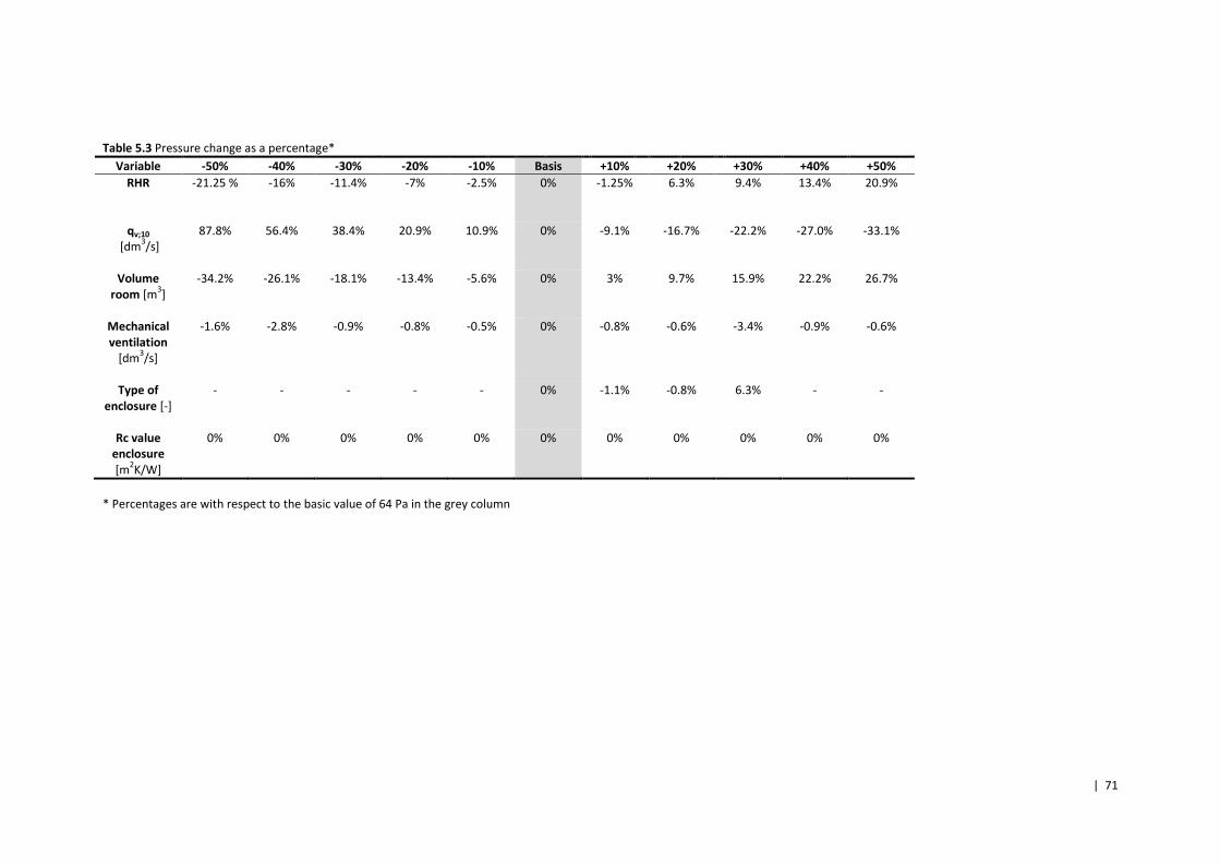
| 71
Table 5.3 Pressure change as a percentage*
Variable -50% -40% -30% -20% -10% Basis +10% +20% +30% +40% +50%
RHR -21.25 % -16% -11.4% -7% -2.5% 0% -1.25% 6.3% 9.4% 13.4% 20.9%
qv;10
[dm3/s]
87.8% 56.4% 38.4% 20.9% 10.9% 0% -9.1% -16.7% -22.2% -27.0% -33.1%
Volume
room [m3]
-34.2% -26.1% -18.1% -13.4% -5.6% 0% 3% 9.7% 15.9% 22.2% 26.7%
Mechanical
ventilation
[dm3/s]
-1.6% -2.8% -0.9% -0.8% -0.5% 0% -0.8% -0.6% -3.4% -0.9% -0.6%
Type of
enclosure [-]
- - - - - 0% -1.1% -0.8% 6.3% - -
Rc value
enclosure
[m2K/W]
0% 0% 0% 0% 0% 0% 0% 0% 0% 0% 0%
* Percentages are with respect to the basic value of 64 Pa in the grey column
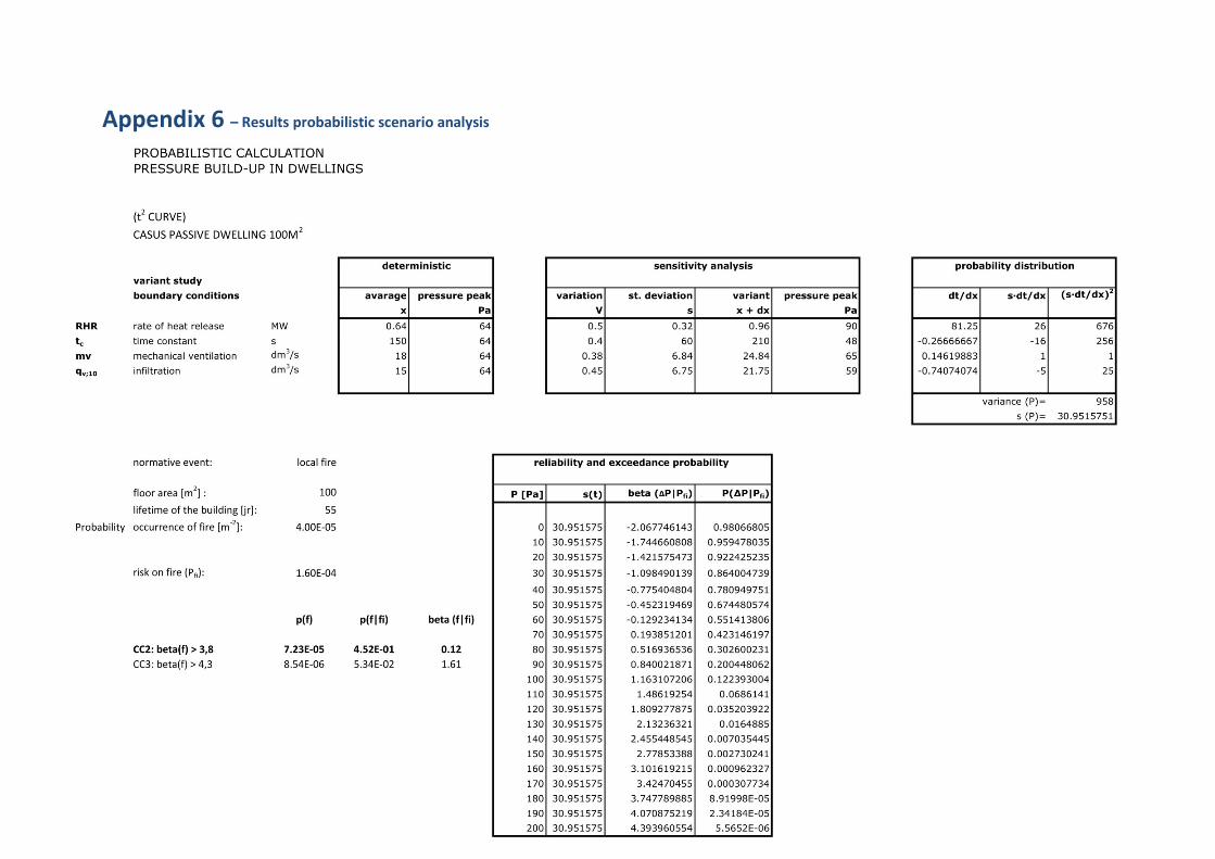
72 |
Appendix 6 – Results probabilistic scenario analysis
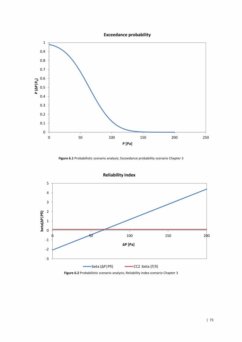
| 73
Figure 6.1 Probabilistic scenario analysis; Exceedance probability scenario Chapter 3
Figure 6.2 Probabilistic scenario analysis; Reliability index scenario Chapter 3
0
0.1
0.2
0.3
0.4
0.5
0.6
0.7
0.8
0.9
1
0 50 100 150 200 250
P (
ΔP
|P
fi)
P [Pa]
Exceedance probability
-3
-2
-1
0
1
2
3
4
5
0 50 100 150 200
be
ta(Δ
P|
Pfi
)
ΔP [Pa]
Reliability index
beta (ΔP|Pfi) CC2 :beta (f|fi)
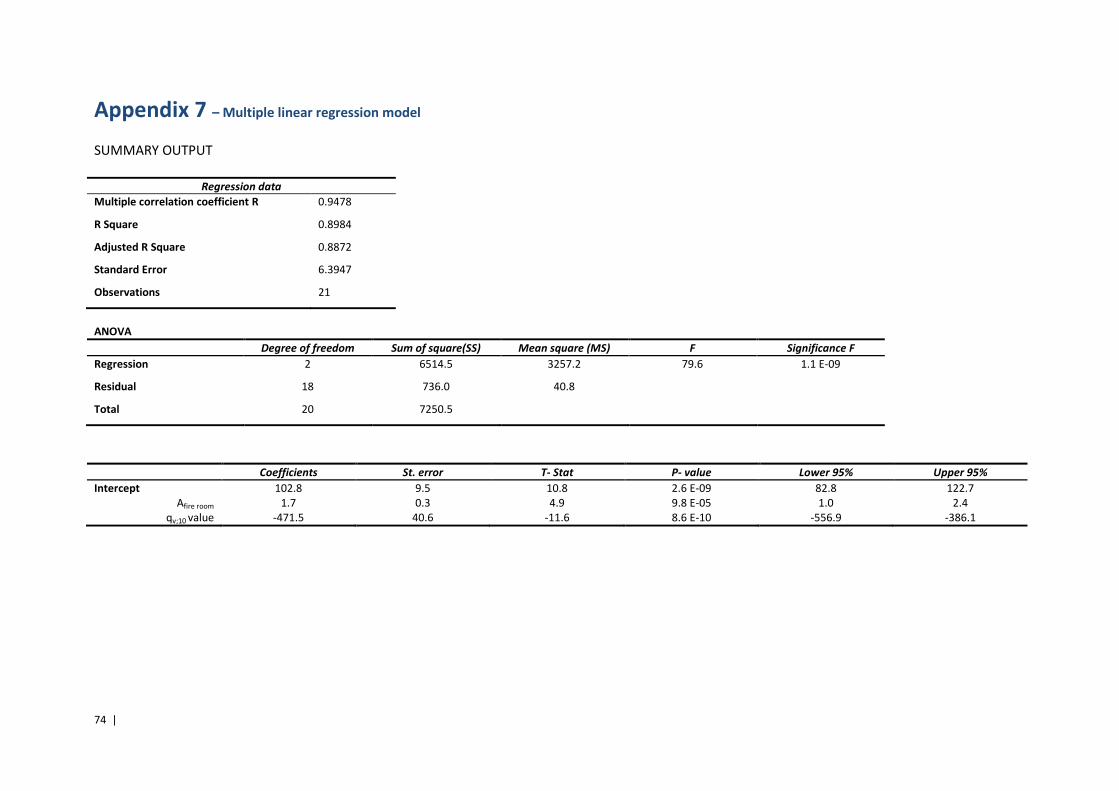
74 |
Appendix 7 – Multiple linear regression model
SUMMARY OUTPUT
Regression data
Multiple correlation coefficient R 0.9478
R Square 0.8984
Adjusted R Square 0.8872
Standard Error 6.3947
Observations 21
ANOVA
Degree of freedom Sum of square(SS) Mean square (MS) F Significance F
Regression 2 6514.5 3257.2 79.6 1.1 E-09
Residual 18 736.0 40.8
Total 20 7250.5
Coefficients St. error T- Stat P- value Lower 95% Upper 95%
Intercept 102.8 9.5 10.8 2.6 E-09 82.8 122.7
Afire room 1.7 0.3 4.9 9.8 E-05 1.0 2.4
qv;10 value -471.5 40.6 -11.6 8.6 E-10 -556.9 -386.1
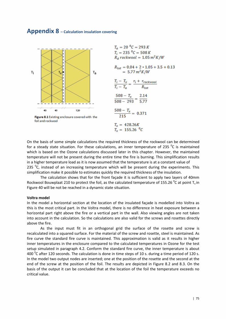
| 75
Appendix 8 – Calculation insulation covering
On the basis of some simple calculations the required thickness of the rockwool can be determined
for a steady state situation. For these calculations, an inner temperature of 235 0C is maintained
which is based on the Ozone calculations discussed later in this chapter. However, the maintained
temperature will not be present during the entire time the fire is burning. This simplification results
in a higher temperature load as it is now assumed that the temperature is at a constant value of
235 0C, instead of an increasing temperature which will be present during the experiments. This
simplification make it possible to estimates quickly the required thickness of the insulation.
The calculation shows that for the front façade it is sufficient to apply two layers of 40mm
Rockwool Bouwplaat 210 to protect the foil, as the calculated temperature of 155.26 0C at point Tx in
Figure 40 will be not be reached in a dynamic state situation.
Voltra model
In the model a horizontal section at the location of the insulated façade is modelled into Voltra as
this is the most critical part. In the Voltra model, there is no difference in heat exposure between a
horizontal part right above the fire or a vertical part in the wall. Also viewing angles are not taken
into account in the calculation. So the calculations are also valid for the screws and rosettes directly
above the fire.
As the input must fit in an orthogonal grid the surface of the rosette and screw is
recalculated into a squared surface. For the material of the screw and rosette, steel is maintained. As
fire curve the standard fire curve is maintained. This approximation is valid as it results in higher
inner temperatures in the enclosure compared to the calculated temperatures in Ozone for the test
setup simulated in paragraph 4.2. Conform the standard fire curve, the inner temperature is about
400 0C after 120 seconds. The calculation is done in time steps of 10 s. during a time period of 120 s.
In the model two output nodes are inserted; one at the position of the rosette and the second at the
end of the screw at the position of the foil. The results are depicted in Figure 8.2 and 8.3. On the
basis of the output it can be concluded that at the location of the foil the temperature exceeds no
critical value.
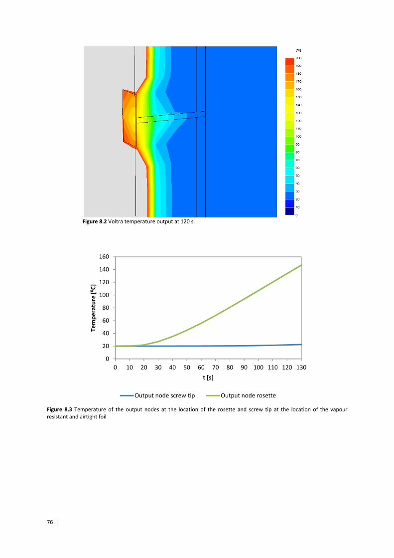
76 |
Figure 8.2 Voltra temperature output at 120 s.
Figure 8.3 Temperature of the output nodes at the location of the rosette and screw tip at the location of the vapour
resistant and airtight foil
0
20
40
60
80
100
120
140
160
0 10 20 30 40 50 60 70 80 90 100 110 120 130
Te
mp
era
ture
[0C
]
t [s]
Output node screw tip Output node rosette
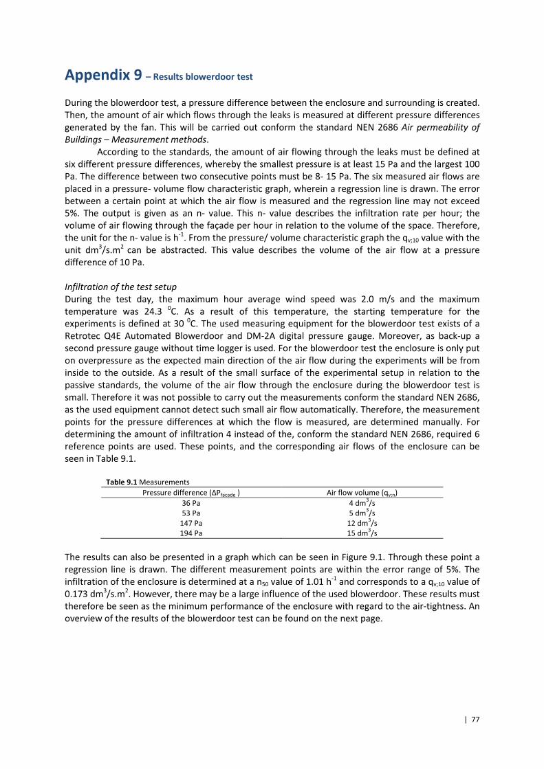
| 77
Appendix 9 – Results blowerdoor test
During the blowerdoor test, a pressure difference between the enclosure and surrounding is created.
Then, the amount of air which flows through the leaks is measured at different pressure differences
generated by the fan. This will be carried out conform the standard NEN 2686 Air permeability of
Buildings – Measurement methods.
According to the standards, the amount of air flowing through the leaks must be defined at
six different pressure differences, whereby the smallest pressure is at least 15 Pa and the largest 100
Pa. The difference between two consecutive points must be 8- 15 Pa. The six measured air flows are
placed in a pressure- volume flow characteristic graph, wherein a regression line is drawn. The error
between a certain point at which the air flow is measured and the regression line may not exceed
5%. The output is given as an n- value. This n- value describes the infiltration rate per hour; the
volume of air flowing through the façade per hour in relation to the volume of the space. Therefore,
the unit for the n- value is h-1
. From the pressure/ volume characteristic graph the qv;10 value with the
unit dm3/s.m
2 can be abstracted. This value describes the volume of the air flow at a pressure
difference of 10 Pa.
Infiltration of the test setup
During the test day, the maximum hour average wind speed was 2.0 m/s and the maximum
temperature was 24.3 0C. As a result of this temperature, the starting temperature for the
experiments is defined at 30 0C. The used measuring equipment for the blowerdoor test exists of a
Retrotec Q4E Automated Blowerdoor and DM-2A digital pressure gauge. Moreover, as back-up a
second pressure gauge without time logger is used. For the blowerdoor test the enclosure is only put
on overpressure as the expected main direction of the air flow during the experiments will be from
inside to the outside. As a result of the small surface of the experimental setup in relation to the
passive standards, the volume of the air flow through the enclosure during the blowerdoor test is
small. Therefore it was not possible to carry out the measurements conform the standard NEN 2686,
as the used equipment cannot detect such small air flow automatically. Therefore, the measurement
points for the pressure differences at which the flow is measured, are determined manually. For
determining the amount of infiltration 4 instead of the, conform the standard NEN 2686, required 6
reference points are used. These points, and the corresponding air flows of the enclosure can be
seen in Table 9.1.
Table 9.1 Measurements
Pressure difference (ΔPfacade ) Air flow volume (qv;n)
36 Pa 4 dm3/s
53 Pa 5 dm3/s
147 Pa 12 dm3/s
194 Pa 15 dm3/s
The results can also be presented in a graph which can be seen in Figure 9.1. Through these point a
regression line is drawn. The different measurement points are within the error range of 5%. The
infiltration of the enclosure is determined at a n50 value of 1.01 h-1
and corresponds to a qv;10 value of
0.173 dm3/s.m
2. However, there may be a large influence of the used blowerdoor. These results must
therefore be seen as the minimum performance of the enclosure with regard to the air-tightness. An
overview of the results of the blowerdoor test can be found on the next page.
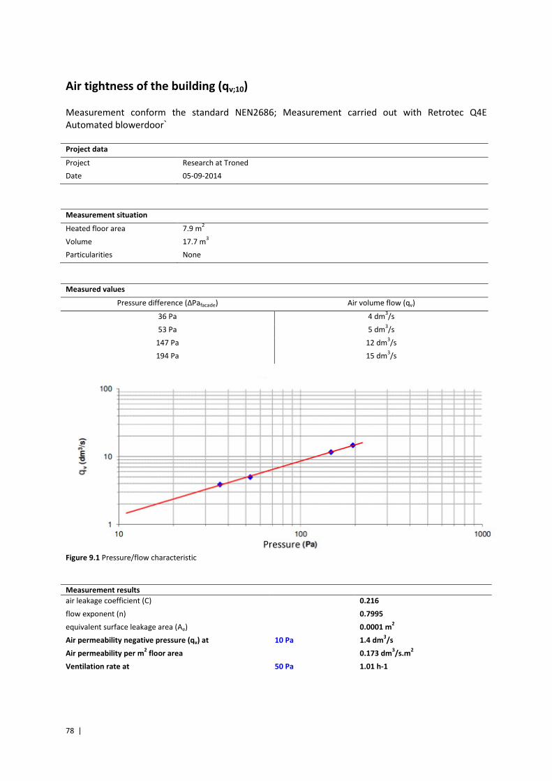
78 |
Air tightness of the building (qv;10)
Measurement conform the standard NEN2686; Measurement carried out with Retrotec Q4E
Automated blowerdoor`
Project data
Project Research at Troned
Date 05-09-2014
Measurement situation
Heated floor area 7.9 m2
Volume 17.7 m3
Particularities None
Measured values
Pressure difference (ΔPafacade) Air volume flow (qv)
36 Pa 4 dm3/s
53 Pa 5 dm3/s
147 Pa 12 dm3/s
194 Pa 15 dm3/s
Figure 9.1 Pressure/flow characteristic
Measurement results
air leakage coefficient (C) 0.216
flow exponent (n) 0.7995
equivalent surface leakage area (Ae) 0.0001 m2
Air permeability negative pressure (qv) at 10 Pa 1.4 dm3/s
Air permeability per m2 floor area 0.173 dm
3/s.m
2
Ventilation rate at 50 Pa 1.01 h-1
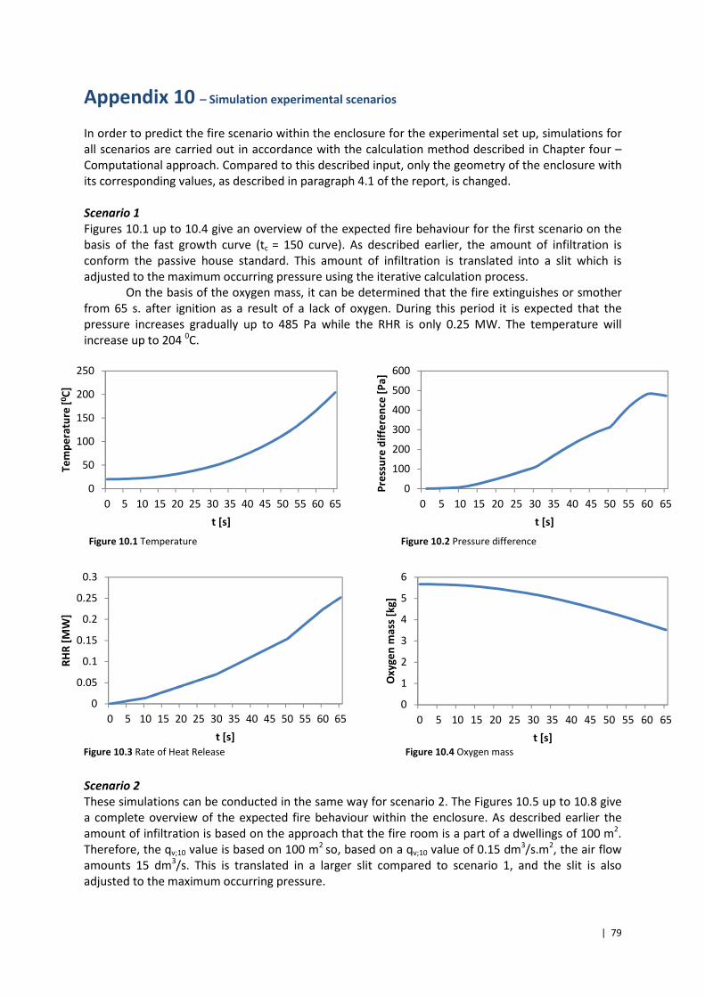
| 79
Appendix 10 – Simulation experimental scenarios
In order to predict the fire scenario within the enclosure for the experimental set up, simulations for
all scenarios are carried out in accordance with the calculation method described in Chapter four –
Computational approach. Compared to this described input, only the geometry of the enclosure with
its corresponding values, as described in paragraph 4.1 of the report, is changed.
Scenario 1
Figures 10.1 up to 10.4 give an overview of the expected fire behaviour for the first scenario on the
basis of the fast growth curve (tc = 150 curve). As described earlier, the amount of infiltration is
conform the passive house standard. This amount of infiltration is translated into a slit which is
adjusted to the maximum occurring pressure using the iterative calculation process.
On the basis of the oxygen mass, it can be determined that the fire extinguishes or smother
from 65 s. after ignition as a result of a lack of oxygen. During this period it is expected that the
pressure increases gradually up to 485 Pa while the RHR is only 0.25 MW. The temperature will
increase up to 204 0C.
Scenario 2
These simulations can be conducted in the same way for scenario 2. The Figures 10.5 up to 10.8 give
a complete overview of the expected fire behaviour within the enclosure. As described earlier the
amount of infiltration is based on the approach that the fire room is a part of a dwellings of 100 m2.
Therefore, the qv;10 value is based on 100 m2
so, based on a qv;10 value of 0.15 dm3/s.m
2, the air flow
amounts 15 dm3/s. This is translated in a larger slit compared to scenario 1, and the slit is also
adjusted to the maximum occurring pressure.
0
0.05
0.1
0.15
0.2
0.25
0.3
0 5 10 15 20 25 30 35 40 45 50 55 60 65
RH
R [
MW
]
t [s]
0
50
100
150
200
250
0 5 10 15 20 25 30 35 40 45 50 55 60 65
Te
mp
era
ture
[0C
]
t [s]
0
100
200
300
400
500
600
0 5 10 15 20 25 30 35 40 45 50 55 60 65
Pre
ssu
re d
iffe
ren
ce [
Pa
]
t [s]
0
1
2
3
4
5
6
0 5 10 15 20 25 30 35 40 45 50 55 60 65
Ox
yg
en
ma
ss [
kg
]
t [s]
Figure 10.1 Temperature Figure 10.2 Pressure difference
Figure 10.3 Rate of Heat Release Figure 10.4 Oxygen mass
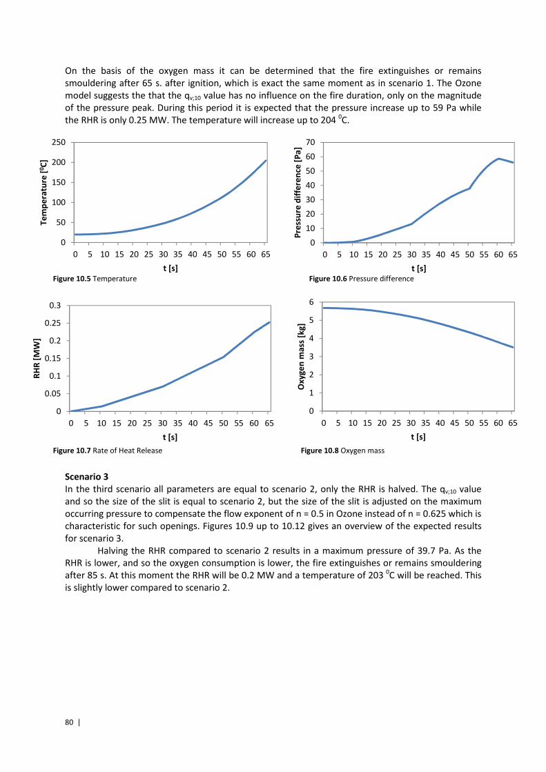
80 |
On the basis of the oxygen mass it can be determined that the fire extinguishes or remains
smouldering after 65 s. after ignition, which is exact the same moment as in scenario 1. The Ozone
model suggests the that the qv;10 value has no influence on the fire duration, only on the magnitude
of the pressure peak. During this period it is expected that the pressure increase up to 59 Pa while
the RHR is only 0.25 MW. The temperature will increase up to 204 0C.
Scenario 3
In the third scenario all parameters are equal to scenario 2, only the RHR is halved. The qv;10 value
and so the size of the slit is equal to scenario 2, but the size of the slit is adjusted on the maximum
occurring pressure to compensate the flow exponent of n = 0.5 in Ozone instead of n = 0.625 which is
characteristic for such openings. Figures 10.9 up to 10.12 gives an overview of the expected results
for scenario 3.
Halving the RHR compared to scenario 2 results in a maximum pressure of 39.7 Pa. As the
RHR is lower, and so the oxygen consumption is lower, the fire extinguishes or remains smouldering
after 85 s. At this moment the RHR will be 0.2 MW and a temperature of 203 0C will be reached. This
is slightly lower compared to scenario 2.
0
1
2
3
4
5
6
0 5 10 15 20 25 30 35 40 45 50 55 60 65
Ox
yg
en
ma
ss [
kg
]
t [s]
0
0.05
0.1
0.15
0.2
0.25
0.3
0 5 10 15 20 25 30 35 40 45 50 55 60 65
RH
R [
MW
]
t [s]
0
10
20
30
40
50
60
70
0 5 10 15 20 25 30 35 40 45 50 55 60 65
Pre
ssu
re d
iffe
ren
ce [
Pa
]
t [s]
0
50
100
150
200
250
0 5 10 15 20 25 30 35 40 45 50 55 60 65
Te
mp
era
ture
[0C
]
t [s]Figure 10.5 Temperature Figure 10.6 Pressure difference
Figure 10.7 Rate of Heat Release Figure 10.8 Oxygen mass
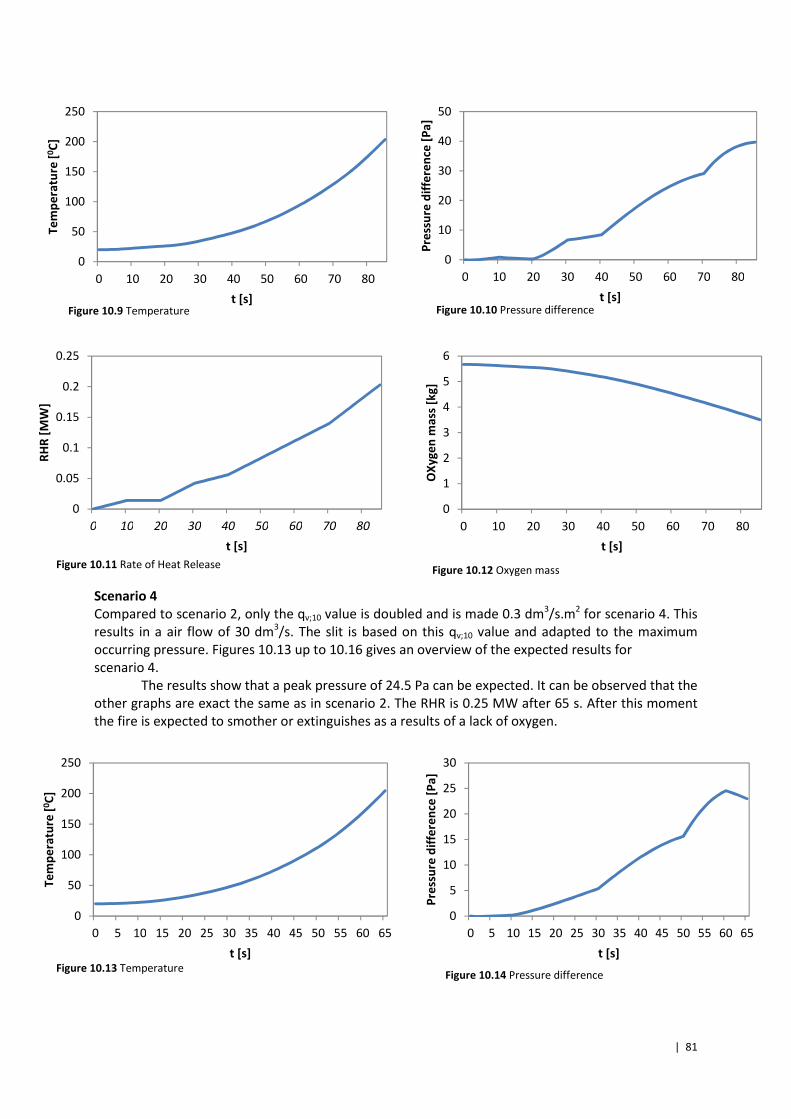
| 81
Scenario 4
Compared to scenario 2, only the qv;10 value is doubled and is made 0.3 dm3/s.m
2 for scenario 4. This
results in a air flow of 30 dm3/s. The slit is based on this qv;10 value and adapted to the maximum
occurring pressure. Figures 10.13 up to 10.16 gives an overview of the expected results for
scenario 4.
The results show that a peak pressure of 24.5 Pa can be expected. It can be observed that the
other graphs are exact the same as in scenario 2. The RHR is 0.25 MW after 65 s. After this moment
the fire is expected to smother or extinguishes as a results of a lack of oxygen.
0
1
2
3
4
5
6
0 10 20 30 40 50 60 70 80
OX
yg
en
ma
ss [
kg
]
t [s]
0
0.05
0.1
0.15
0.2
0.25
0 10 20 30 40 50 60 70 80
RH
R [
MW
]
t [s]
0
10
20
30
40
50
0 10 20 30 40 50 60 70 80
Pre
ssu
re d
iffe
ren
ce [
Pa
]
t [s]
0
50
100
150
200
250
0 10 20 30 40 50 60 70 80
Te
mp
era
ture
[0C
]
t [s]
0
5
10
15
20
25
30
0 5 10 15 20 25 30 35 40 45 50 55 60 65
Pre
ssu
re d
iffe
ren
ce [
Pa
]
t [s]
0
50
100
150
200
250
0 5 10 15 20 25 30 35 40 45 50 55 60 65
Te
mp
era
ture
[0C
]
t [s]
Figure 10.9 Temperature Figure 10.10 Pressure difference
Figure 10.11 Rate of Heat Release Figure 10.12 Oxygen mass
Figure 10.13 Temperature Figure 10.14 Pressure difference
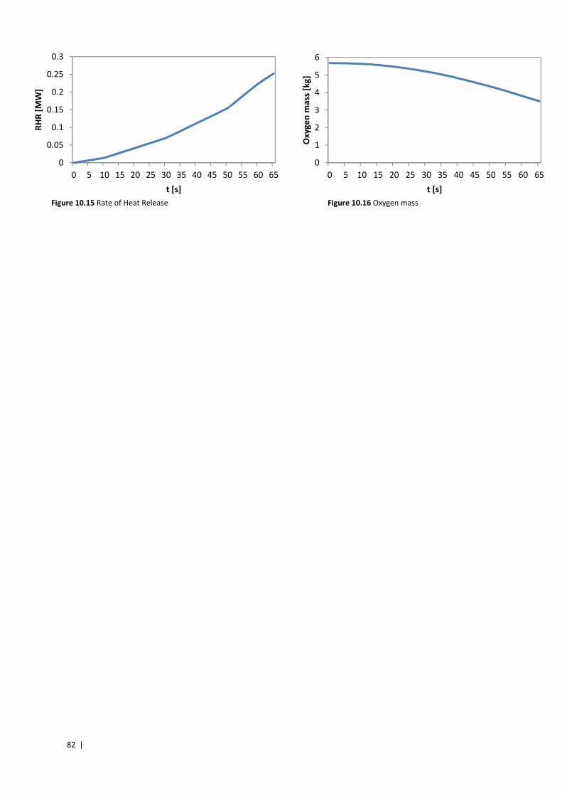
82 |
0
1
2
3
4
5
6
0 5 10 15 20 25 30 35 40 45 50 55 60 65
Ox
yg
en
ma
ss [
kg
]
t [s]
0
0.05
0.1
0.15
0.2
0.25
0.3
0 5 10 15 20 25 30 35 40 45 50 55 60 65
RH
R [
MW
]
t [s]
Figure 10.15 Rate of Heat Release Figure 10.16 Oxygen mass
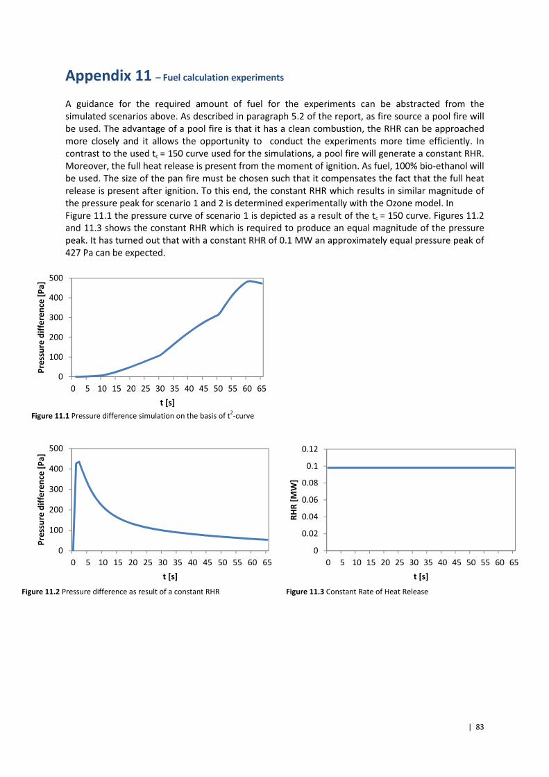
| 83
Appendix 11 – Fuel calculation experiments
A guidance for the required amount of fuel for the experiments can be abstracted from the
simulated scenarios above. As described in paragraph 5.2 of the report, as fire source a pool fire will
be used. The advantage of a pool fire is that it has a clean combustion, the RHR can be approached
more closely and it allows the opportunity to conduct the experiments more time efficiently. In
contrast to the used tc = 150 curve used for the simulations, a pool fire will generate a constant RHR.
Moreover, the full heat release is present from the moment of ignition. As fuel, 100% bio-ethanol will
be used. The size of the pan fire must be chosen such that it compensates the fact that the full heat
release is present after ignition. To this end, the constant RHR which results in similar magnitude of
the pressure peak for scenario 1 and 2 is determined experimentally with the Ozone model. In
Figure 11.1 the pressure curve of scenario 1 is depicted as a result of the tc = 150 curve. Figures 11.2
and 11.3 shows the constant RHR which is required to produce an equal magnitude of the pressure
peak. It has turned out that with a constant RHR of 0.1 MW an approximately equal pressure peak of
427 Pa can be expected.
0
0.02
0.04
0.06
0.08
0.1
0.12
0 5 10 15 20 25 30 35 40 45 50 55 60 65
RH
R [
MW
]
t [s]
0
100
200
300
400
500
0 5 10 15 20 25 30 35 40 45 50 55 60 65
Pre
ssu
re d
iffe
ren
ce [
Pa
]
t [s]
0
100
200
300
400
500
0 5 10 15 20 25 30 35 40 45 50 55 60 65
Pre
ssu
re d
iffe
ren
ce [
Pa
]
t [s]
Figure 11.1 Pressure difference simulation on the basis of t2-curve
Figure 11.2 Pressure difference as result of a constant RHR Figure 11.3 Constant Rate of Heat Release
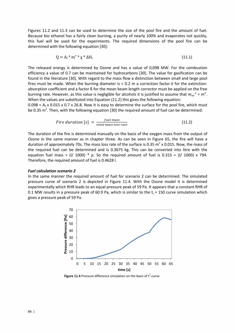
84 |
Figures 11.2 and 11.3 can be used to determine the size of the pool fire and the amount of fuel.
Because bio ethanol has a fairly clean burning, a purity of nearly 100% and evaporates not quickly,
this fuel will be used for the experiments. The required dimensions of the pool fire can be
determined with the following equation [30]:
Q = Af * m” * χ * ΔHc (11.1)
The released energy is determined by Ozone and has a value of 0,098 MW. For the combustion
efficiency a value of 0.7 can be maintained for hydrocarbons [30]. The value for gasification can be
found in the literature [30]. With regard to the mass flow a distinction between small and large pool
fires must be made. When the burning diameter is < 0.2 m a correction factor k for the extinction-
absorption coefficient and a factor ß for the mean beam length corrector must be applied on the free
burning rate. However, as this value is negligible for alcohols it is justified to assume that @�” = m”.
When the values are substituted into Equation (11.2) this gives the following equation:
0.098 = Af x 0.015 x 0.7 x 26.8. Now it is easy to determine the surface for the pool fire, which must
be 0.35 m2. Then, with the following equation [30] the required amount of fuel can be determined:
�����!�#��}[[~] = T�G�no��]t]o�no���t��so]G (11.2)
The duration of the fire is determined manually on the basis of the oxygen mass from the output of
Ozone in the same manner as in chapter three. As can be seen in Figure 65, the fire will have a
duration of approximately 70s. The mass loss rate of the surface is 0.35 m2 x 0.015. Now, the mass of
the required fuel can be determined and is 0.3675 kg. This can be converted into litre with the
equation fuel mass = (l/ 1000) * ρ. So the required amount of fuel is 0.315 = (l/ 1000) x 794.
Therefore, the required amount of fuel is 0.4628 l.
Fuel calculation scenario 2
In the same manner the required amount of fuel for scenario 2 can be determined. The simulated
pressure curve of scenario 2 is depicted in Figure 11.4. With the Ozone model it is determined
experimentally which RHR leads to an equal pressure peak of 59 Pa. It appears that a constant RHR of
0.1 MW results in a pressure peak of 60.9 Pa, which is similar to the tc = 150 curve simulation which
gives a pressure peak of 59 Pa.
0
10
20
30
40
50
60
70
0 5 10 15 20 25 30 35 40 45 50 55 60 65
Pre
ssu
re d
iffe
ren
ce [
Pa
]
time [s]
Figure 11.4 Pressure difference simulation on the basis of t2-curve
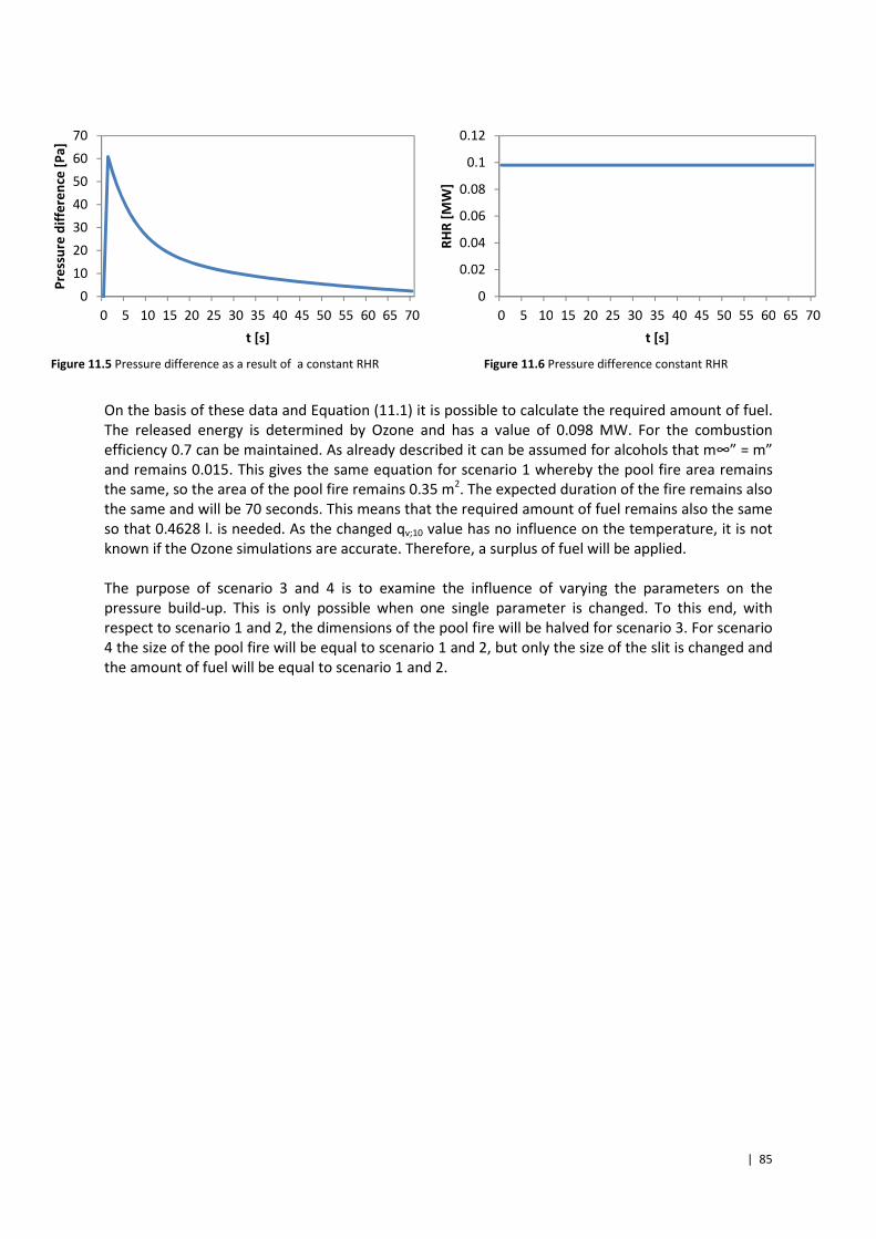
| 85
On the basis of these data and Equation (11.1) it is possible to calculate the required amount of fuel.
The released energy is determined by Ozone and has a value of 0.098 MW. For the combustion
efficiency 0.7 can be maintained. As already described it can be assumed for alcohols that m∞” = m”
and remains 0.015. This gives the same equation for scenario 1 whereby the pool fire area remains
the same, so the area of the pool fire remains 0.35 m2. The expected duration of the fire remains also
the same and will be 70 seconds. This means that the required amount of fuel remains also the same
so that 0.4628 l. is needed. As the changed qv;10 value has no influence on the temperature, it is not
known if the Ozone simulations are accurate. Therefore, a surplus of fuel will be applied.
The purpose of scenario 3 and 4 is to examine the influence of varying the parameters on the
pressure build-up. This is only possible when one single parameter is changed. To this end, with
respect to scenario 1 and 2, the dimensions of the pool fire will be halved for scenario 3. For scenario
4 the size of the pool fire will be equal to scenario 1 and 2, but only the size of the slit is changed and
the amount of fuel will be equal to scenario 1 and 2.
0
0.02
0.04
0.06
0.08
0.1
0.12
0 5 10 15 20 25 30 35 40 45 50 55 60 65 70
RH
R [
MW
]
t [s]
0
10
20
30
40
50
60
70
0 5 10 15 20 25 30 35 40 45 50 55 60 65 70
Pre
ssu
re d
iffe
ren
ce [
Pa
]
t [s]
Figure 11.6 Pressure difference constant RHR Figure 11.5 Pressure difference as a result of a constant RHR
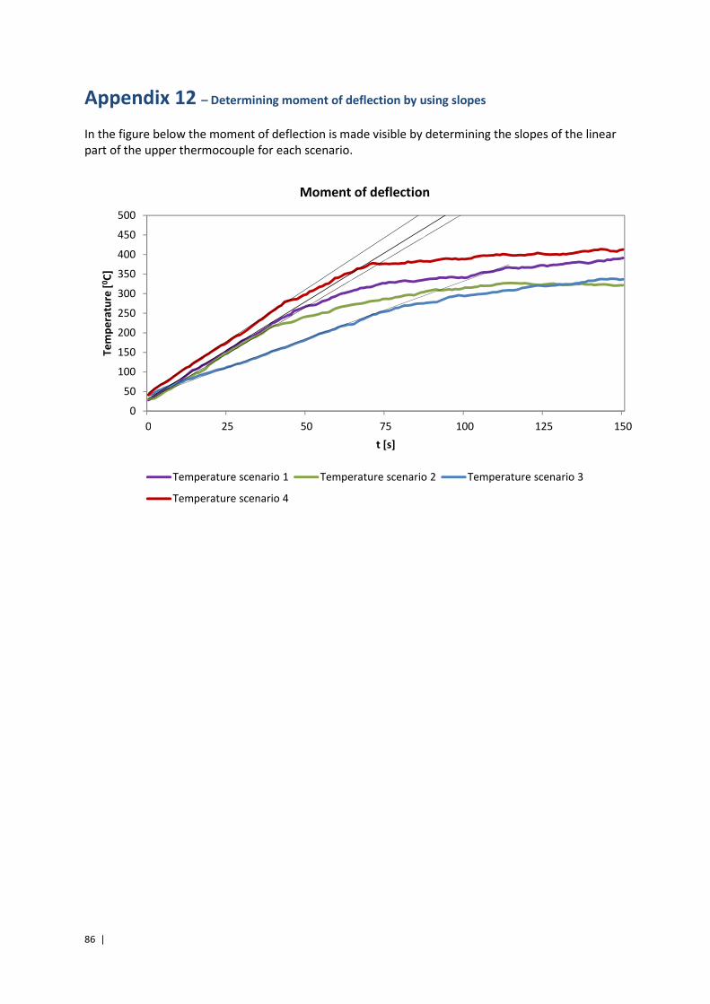
86 |
Appendix 12 – Determining moment of deflection by using slopes
In the figure below the moment of deflection is made visible by determining the slopes of the linear
part of the upper thermocouple for each scenario.
0
50
100
150
200
250
300
350
400
450
500
0 25 50 75 100 125 150
Te
mp
era
ture
[0C
]
t [s]
Moment of deflection
Temperature scenario 1 Temperature scenario 2 Temperature scenario 3
Temperature scenario 4 RC line 1 RC line 2
RC line 3 RC line 4
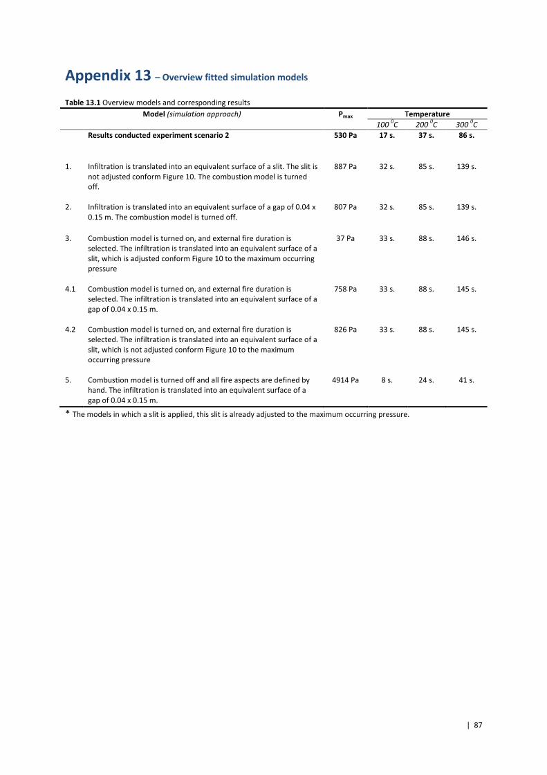
| 87
Appendix 13 – Overview fitted simulation models Table 13.1 Overview models and corresponding results
Model (simulation approach) Pmax Temperature
100 0C
200
0C 300
0C
Results conducted experiment scenario 2 530 Pa 17 s. 37 s. 86 s.
1. Infiltration is translated into an equivalent surface of a slit. The slit is
not adjusted conform Figure 10. The combustion model is turned
off.
887 Pa 32 s. 85 s. 139 s.
2. Infiltration is translated into an equivalent surface of a gap of 0.04 x
0.15 m. The combustion model is turned off.
807 Pa 32 s. 85 s. 139 s.
3. Combustion model is turned on, and external fire duration is
selected. The infiltration is translated into an equivalent surface of a
slit, which is adjusted conform Figure 10 to the maximum occurring
pressure
37 Pa 33 s. 88 s. 146 s.
4.1 Combustion model is turned on, and external fire duration is
selected. The infiltration is translated into an equivalent surface of a
gap of 0.04 x 0.15 m.
758 Pa 33 s. 88 s. 145 s.
4.2 Combustion model is turned on, and external fire duration is
selected. The infiltration is translated into an equivalent surface of a
slit, which is not adjusted conform Figure 10 to the maximum
occurring pressure
826 Pa 33 s. 88 s. 145 s.
5. Combustion model is turned off and all fire aspects are defined by
hand. The infiltration is translated into an equivalent surface of a
gap of 0.04 x 0.15 m.
4914 Pa 8 s. 24 s. 41 s.
* The models in which a slit is applied, this slit is already adjusted to the maximum occurring pressure.
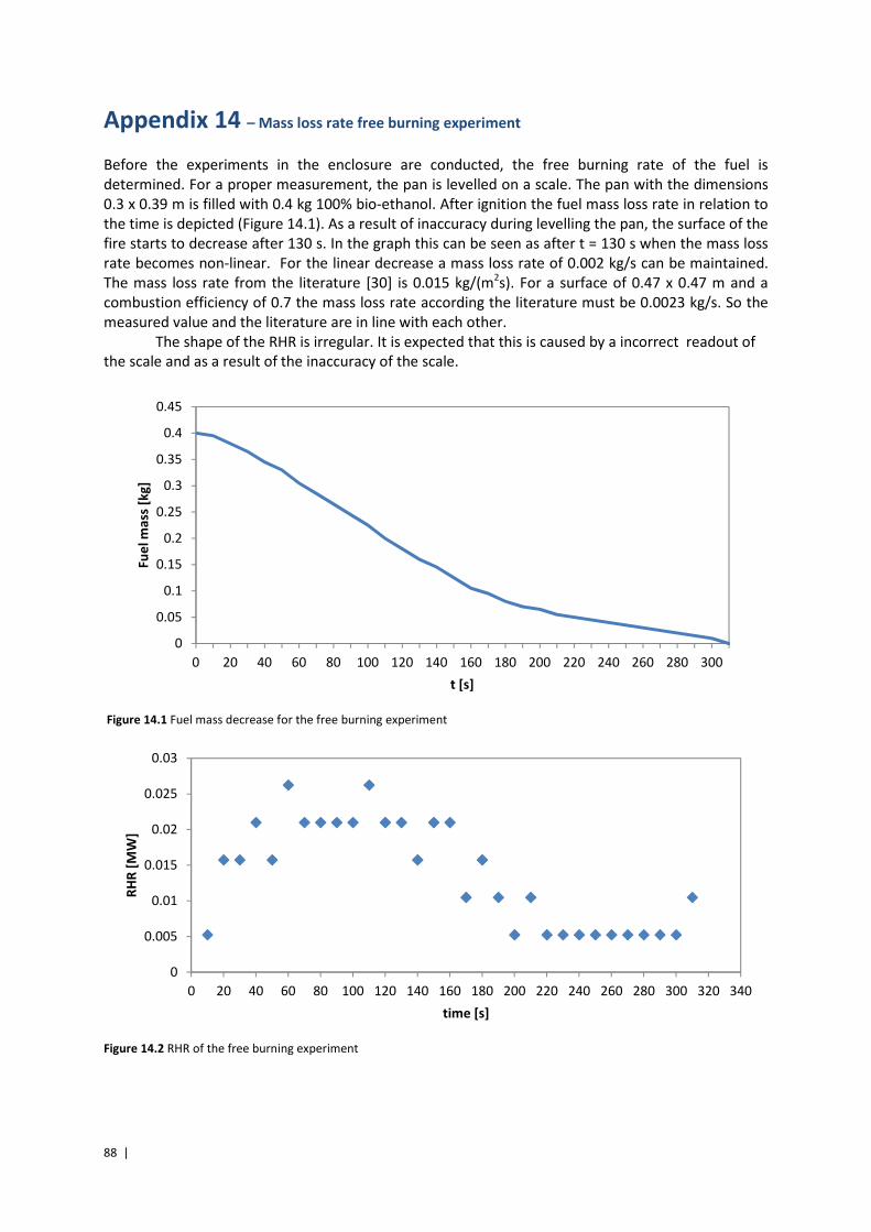
88 |
Appendix 14 – Mass loss rate free burning experiment
Before the experiments in the enclosure are conducted, the free burning rate of the fuel is
determined. For a proper measurement, the pan is levelled on a scale. The pan with the dimensions
0.3 x 0.39 m is filled with 0.4 kg 100% bio-ethanol. After ignition the fuel mass loss rate in relation to
the time is depicted (Figure 14.1). As a result of inaccuracy during levelling the pan, the surface of the
fire starts to decrease after 130 s. In the graph this can be seen as after t = 130 s when the mass loss
rate becomes non-linear. For the linear decrease a mass loss rate of 0.002 kg/s can be maintained.
The mass loss rate from the literature [30] is 0.015 kg/(m2s). For a surface of 0.47 x 0.47 m and a
combustion efficiency of 0.7 the mass loss rate according the literature must be 0.0023 kg/s. So the
measured value and the literature are in line with each other.
The shape of the RHR is irregular. It is expected that this is caused by a incorrect readout of
the scale and as a result of the inaccuracy of the scale.
Figure 14.1 Fuel mass decrease for the free burning experiment
Figure 14.2 RHR of the free burning experiment
0
0.05
0.1
0.15
0.2
0.25
0.3
0.35
0.4
0.45
0 20 40 60 80 100 120 140 160 180 200 220 240 260 280 300
Fu
el
ma
ss [
kg
]
t [s]
0
0.005
0.01
0.015
0.02
0.025
0.03
0 20 40 60 80 100 120 140 160 180 200 220 240 260 280 300 320 340
RH
R [
MW
]
time [s]
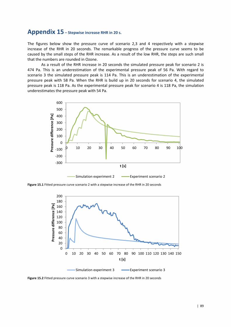
| 89
Appendix 15 – Stepwise increase RHR in 20 s.
The figures below show the pressure curve of scenario 2,3 and 4 respectively with a stepwise
increase of the RHR in 20 seconds. The remarkable progress of the pressure curve seems to be
caused by the small steps of the RHR increase. As a result of the low RHR, the steps are such small
that the numbers are rounded in Ozone.
As a result of the RHR increase in 20 seconds the simulated pressure peak for scenario 2 is
474 Pa. This is an underestimation of the experimental pressure peak of 56 Pa. With regard to
scenario 3 the simulated pressure peak is 114 Pa. This is an underestimation of the experimental
pressure peak with 58 Pa. When the RHR is build up in 20 seconds for scenario 4, the simulated
pressure peak is 118 Pa. As the experimental pressure peak for scenario 4 is 118 Pa, the simulation
underestimates the pressure peak with 54 Pa.
Figure 15.1 Fitted pressure curve scenario 2 with a stepwise increase of the RHR in 20 seconds
Figure 15.2 Fitted pressure curve scenario 3 with a stepwise increase of the RHR in 20 seconds
-300
-200
-100
0
100
200
300
400
500
600
0 10 20 30 40 50 60 70 80 90 100
Pre
ssu
re d
iffe
ren
ce [
Pa
]
t [s]
Simulation experiment 2 Experiment scenario 2
0
20
40
60
80
100
120
140
160
180
200
0 10 20 30 40 50 60 70 80 90 100 110 120 130 140 150
Pre
ssu
re d
iffe
ren
ce [
Pa
]
t [s]
Simulation experiment 3 Experiment scenario 3
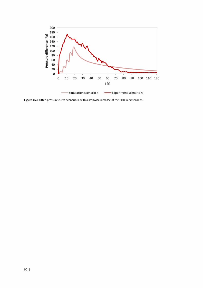
90 |
Figure 15.3 Fitted pressure curve scenario 4 with a stepwise increase of the RHR in 20 seconds
0
20
40
60
80
100
120
140
160
180
200
0 10 20 30 40 50 60 70 80 90 100 110 120
Pre
ssu
re d
iffe
ren
ce [
Pa
]
t [s]
Simulation scenario 4 Experiment scenario 4
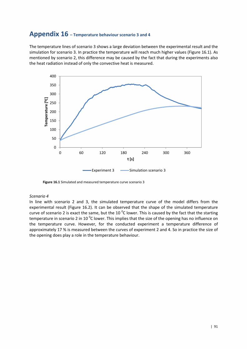
| 91
Appendix 16 – Temperature behaviour scenario 3 and 4
The temperature lines of scenario 3 shows a large deviation between the experimental result and the
simulation for scenario 3. In practice the temperature will reach much higher values (Figure 16.1). As
mentioned by scenario 2, this difference may be caused by the fact that during the experiments also
the heat radiation instead of only the convective heat is measured.
Scenario 4
In line with scenario 2 and 3, the simulated temperature curve of the model differs from the
experimental result (Figure 16.2). It can be observed that the shape of the simulated temperature
curve of scenario 2 is exact the same, but the 10 0C lower. This is caused by the fact that the starting
temperature in scenario 2 in 10 0C lower. This implies that the size of the opening has no influence on
the temperature curve. However, for the conducted experiment a temperature difference of
approximately 17 % is measured between the curves of experiment 2 and 4. So in practice the size of
the opening does play a role in the temperature behaviour.
0
50
100
150
200
250
300
350
400
0 60 120 180 240 300 360
Te
mp
era
ture
[0C
]
t [s]
Experiment 3 Simulation scenario 3
Figure 16.1 Simulated and measured temperature curve scenario 3
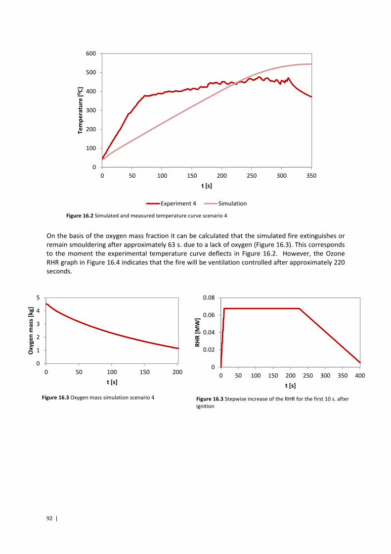
92 |
On the basis of the oxygen mass fraction it can be calculated that the simulated fire extinguishes or
remain smouldering after approximately 63 s. due to a lack of oxygen (Figure 16.3). This corresponds
to the moment the experimental temperature curve deflects in Figure 16.2. However, the Ozone
RHR graph in Figure 16.4 indicates that the fire will be ventilation controlled after approximately 220
seconds.
0
100
200
300
400
500
600
0 50 100 150 200 250 300 350
Te
mp
era
ture
[0C
]
t [s]
Experiment 4 Simulation
Figure 16.2 Simulated and measured temperature curve scenario 4
Figure 16.3 Oxygen mass simulation scenario 4
0
1
2
3
4
5
0 50 100 150 200
Ox
yg
en
ma
ss [
kg
]
t [s]
0
0.02
0.04
0.06
0.08
0 50 100 150 200 250 300 350 400
RH
R [
MW
]
t [s]
Figure 16.3 Stepwise increase of the RHR for the first 10 s. after
ignition

ii |