Embed Size (px)
Citation preview

Firing Costs, Subcontracting and Employment Dynamics∗
Francisca Pérez†
January 2, 2015
Abstract
This paper studies the impact of severance payments on employment when firms can sub-contract as a substitute for hiring workers. In countries with strict job security regulationsfirms use flexible staffing arrangements to buffer the regular workforce from economic fluctu-ations and avoid workers’ firing costs. I set up a general equilibrium model in the tradition ofHopenhayn and Rogerson (1993) where firms can hire subcontractors that are totally flexible,and permanent workers that entail firing costs. Both types are perfect substitutes in pro-duction, but permanent workers are relatively less expensive as subcontractors’ charges arehigher than the firm’s own production costs. I estimate the model using a simulated methodof moments by fitting employment dynamics of Chilean manufacturing plants. I find thatallowing firms to subcontract workers increases output, employment and productivity. Thiseffect is stronger on output as subcontracted workers allow firms to respond more aggressivelyto productivity shocks, which enhances the allocation of labor across firms and hence totalfactor productivity. When firms can subcontract, the negative effects of firing costs are lessthan previously estimated in the literature.
Keywords: Subcontracting, firing costs, reallocation, general equilibrium
∗This paper is based on the main chapter of my Ph.D. dissertation written at Boston University. I thank mythesis committee François Gourio, Simon Gilchrist, Alisdair McKay, and Berardino Palazzo for their helpfulcomments and suggestions, and seminar participants at the Boston University macroeconomic seminar. Allerrors are my own.†For comments and contact please email at [email protected]
1
Firing costs and subcontracting Perez (2014)
1 Introduction
In many countries labor markets are constraint by strict legislations that protect workersagainst arbitrary actions, and give them higher job stability in the face of adverse economicconditions.1 Even when these regulations are necessary in some cases, they also increaselabor adjustment costs and impose heavy constraints to the firms that want to adjust theirworkforce in response to economic fluctuations. As a result, firms are increasingly turningto flexible staffing arrangements with less stringent rules, particularly with regard to firingcosts. These contracts allow firms to buffer the stock of permanent workers, and overcome thepotential costs associated with employment regulations during off-peak periods. As firms’ useof contingent workers widespread, it is important to explicitly take into account this marginof adjustment for firms to properly evaluate the impact of firing costs. This paper provides abasic framework to perform such analysis.
A variety of evidence has pointed to a significant growth of flexible staffing arrangements, inparticular, with regard to subcontracting. Subcontracting is a form of temporary employmentin which a firm (‘main firm’) sublets to a third party (‘subcontract firm’) the performanceof tasks or works, complete or partially, with its own dependent employees. When firmssubcontract tasks to other firms, the employer of record for the worker performing the taskchanges, and the responsibility for all employment liabilities is trespassed to the subcontractfirm. This way the firm avoids potential costs of dismissal and gains flexibility to terminateworkers’ contracts at will. But why then firms don’t subcontract their entire workforce tocircumvent firing costs? The hypothesis explored in this paper is that subcontractors’ chargesare higher than the firm’s own production costs. Recognizing this, firms still hire permanentworkers even when subcontracted workers do not entail firing costs.
Chile provides a particularly interesting setting to investigate the combine effects of firingcosts and subcontracted workers. For many years, the country carried out asymmetric labormarket reforms introducing a two-tier system; supporting job security provisions that greatlypenalized employers for firing workers by imposing sizable tenure-dependent severance pay-ments, while maintaining the market for subcontracted workers practically deregulated. Thispolicy sustained a high employment protection legislation gap between both types of workersfor years, triggering a widespread use of subcontracted workers, and a reallocation away frompermanent workers.2
1Legislation on employment protection usually regulates unfair dismissals, dismissals for economic reasons,mandatory severance payments, the use of fixed-term contracts, and minimum advance notice period in caseof impending dismissal.
2A recent survey of employment conditions conducted by the Labor Directorate in Chile (ENCLA for itsinitials in Spanish) indicates subcontracting has widespread as a form of flexible employment in Chile: 25%of the firms use subcontracted for their main activities, while 38% declare to have subcontracted as least oneservice during 2011. The survey also shows that increasing number of workers is engaged in subcontracted
2
Firing costs and subcontracting Perez (2014)
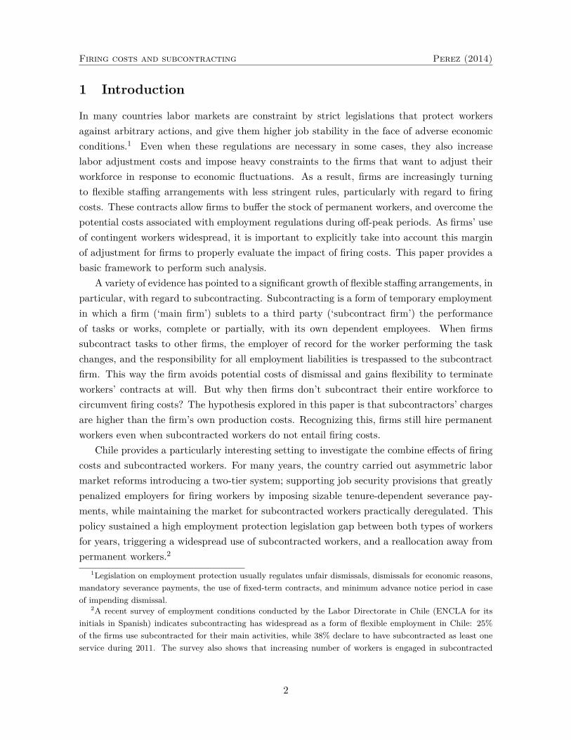
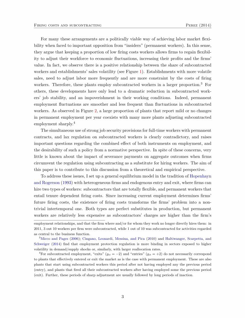
For many these arrangements are a politically viable way of achieving labor market flexi-bility when faced to important opposition from “insiders” (permanent workers). In this sense,they argue that keeping a proportion of low firing costs workers allows firms to regain flexibil-ity to adjust their workforce to economic fluctuations, increasing their profits and the firms’value. In fact, we observe there is a positive relationship between the share of subcontractedworkers and establishments’ sales volatility (see Figure 1). Establishments with more volatilesales, need to adjust labor more frequently and are more constraint by the costs of firingworkers. Therefore, these plants employ subcontracted workers in a larger proportion.3 Forothers, these developments have only lead to a dramatic reduction in subcontracted work-ers’ job stability, and an impoverishment in their working conditions. Indeed, permanentemployment fluctuations are smoother and less frequent than fluctuations in subcontractedworkers. As observed in Figure 2, a large proportion of plants that report mild or no changesin permanent employment per year coexists with many more plants adjusting subcontractedemployment sharply.4
The simultaneous use of strong job security provisions for full-time workers with permanentcontracts, and lax regulation on subcontracted workers is clearly contradictory, and raisesimportant questions regarding the combined effect of both instruments on employment, andthe desirability of such a policy from a normative perspective. In spite of these concerns, verylittle is known about the impact of severance payments on aggregate outcomes when firmscircumvent the regulation using subcontracting as a substitute for hiring workers. The aim ofthis paper is to contribute to this discussion from a theoretical and empirical perspective.
To address these issues, I set up a general equilibrium model in the tradition of Hopenhaynand Rogerson (1993) with heterogeneous firms and endogenous entry and exit, where firms canhire two types of workers: subcontractors that are totally flexible, and permanent workers thatentail tenure dependent firing costs. Since increasing current employment determines firms’future firing costs, the existence of firing costs transforms the firms’ problem into a non-trivial intertemporal one. Both types are perfect substitutes in production, but permanentworkers are relatively less expensive as subcontractors’ charges are higher than the firm’s
employment relationships, and that the firm where and/or for whom they work no longer directly hires them: in2011, 3 out 10 workers per firm were subcontracted, while 1 out of 10 was subcontracted for activities regardedas central to the business function.
3Micco and Pages (2006); Cingano, Leonardi, Messina, and Pica (2010) and Haltiwanger, Scarpetta, andSchweiger (2014) find that employment protection regulation is more binding in sectors exposed to highervolatility in demand/supply shocks or, similarly, with larger reallocation rates.
4For subcontracted employment, “exits” (git = −2) and “entries” (git = +2) do not necessarily correspondto plants that effectively entered or exit the market as is the case with permanent employment. These are alsoplants that start using subcontracted workers this period after not having employed any the previous period(entry), and plants that fired all their subcontracted workers after having employed some the previous period(exit). Further, these periods of sharp adjustment are usually followed by long periods of inaction.
3
Firing costs and subcontracting Perez (2014)
Figure 1: Establishments Sales’ Volatility and Share of Subcontracting
.05
.1.1
5.2
.25
Shar
e of
sub
cont
ract
ing
0 20 40 60 80 100Sales' volatility percentile
Note: Only plants that use subcontracting are considered.
Notes: the figure shows the average share of subcontracted workers in an establishment by decile of salesvolatility. Source: ENIA.
Figure 2: Distribution of Employment Growth Rate
05
1015
2025
Perc
ent
Growth rate interval (width=0.1)
-2-1
.9-1
.8-1
.7-1
.6-1
.5-1
.4-1
.3-1
.2-1
.1 -1 -.9 -.8 -.7 -.6 -.5 -.4 -.3 -.2 -.1 0 .1 .2 .3 .4 .5 .6 .7 .8 .9 11.
11.
21.
31.
41.
51.
61.
71.
81.
9 2
Permanent Employment
05
1015
2025
Perc
ent
Growth rate interval (width=0.1)
-2-1
.9-1
.8-1
.7-1
.6-1
.5-1
.4-1
.3-1
.2-1
.1 -1 -.9 -.8 -.7 -.6 -.5 -.4 -.3 -.2 -.1 0 .1 .2 .3 .4 .5 .6 .7 .8 .9 11.
11.
21.
31.
41.
51.
61.
71.
81.
9 2
Subcontracted Employment
Notes: the figure represents the fraction of plants expanding (contracting) at different growth rate intervals (asmeasured in the horizontal axis). Growth rate is computed according to the standard Davis and Haltiwanger(1992) definitions: git = (xit−xit−1)/(0.5∗ (xit+xit−1)), where xit is the number of employees (subcontractedor permanent) in plant i at time t. The bars to the right of the origin correspond to job creation and to theleft to job destruction. At the center, the proportion of plants for which employment remains unchanged, andexits (entries) correspond to the left (right) endpoint. Source: ENIA.
4

Firing costs and subcontracting Perez (2014)
own production costs. Hence, firms can either hire full-time permanent workers and bearthe potential adjustment costs in case of dismissal, or afford to pay a wage premium onsubcontracted workers and benefit from the flexibility of terminating their contracts at zerocost. When subcontractors’ charges are large enough and all permanent workers are subjectto firing costs, the employment protection system studied in this paper reduces exactly to theseparation tax regime analyzed by Hopenhayn and Rogerson (1993).
For the estimation, I set the model in partial equilibrium and use the Annual NationalManufacturing Survey (ENIA for its initials in Spanish) conducted by the National Instituteof Statistics of Chile (INE), which contains detailed information on subcontracted workers formore than 10,000 plants over the span of seven years. Since the model has no closed-formsolution I use a simulated method of moments, and optimally choose the parameters to re-produce a set of moments that combine time-series employment dynamics, and cross-sectionalindustry characteristics. By studying permanent and subcontracted employment dynamics,I am able to measure the costs of adjusting permanent workers, and the wage premium onsubcontracted workers firms are willing to pay to substitute for permanent workers. The im-portance of incorporating subcontracted workers becomes clear when comparing the differentestimations performed. Finally, I embed my estimated model in a general equilibrium frame-work to quantify the costs of the regulation, and the potential benefits of removing it. Also,I measure the gains from subcontracting as a substitute for hiring workers when firms facestrict job security regulations.
To anticipate my results, I find that severance payments in the manufacturing sector inChile are equivalent to seven months’ wages, and that workers get tenure after 4 years in thejob. Further, firms are willing to pay a wage premium of 10 percent on subcontracted workersto substitute for hiring workers, and be able to buffer the regular workforce from economicfluctuations avoiding workers’ firing costs. A naive researcher wanting to estimate firingcosts in Chilean manufacturing plants without noticing that firms subcontract to substitutefor hiring workers, would conclude that firing costs are substantially lower in the economy(i.e. between one and four months’ wages), and that on average workers get tenure afterapproximately 3 year on the job.
The main finding of the paper is that allowing firms to subcontract workers in a heav-ily regulated environment increases output, employment and productivity. To overcome thepotential costs associated with dismissing permanent workers, firms subcontract as a sub-stitute for hiring workers to buffer the regular workforce from economic fluctuations. Thisway firms smooth out permanent employment fluctuations at the expense of an increase insubcontracted employment volatility. Provided subcontractors’ charges are small relative toadjusting inside workers, subcontracting workers is an attractive alternative for the firms tocover peak demand or productivity shocks. When firms can subcontract they respond moreaggressively to productivity shocks, which enhances the allocation of labor across firms and
5
Firing costs and subcontracting Perez (2014)
hence total factor productivity (TFP). In this context, the negative effects of firing costs onaggregate outcomes are less than previously estimated in the literature. If the government de-cided to eliminate firing costs instead of allowing subcontracting to introduce flexibility to thelabor market, the increase in productivity and output of this policy would be even stronger.However, such a policy would eliminate subcontracted workers, being permanent workers thebig winners of the change.
Related literature This paper is related to the literature that evaluates the impact of jobsecurity provisions on labor markets performance, and productivity. Several models predictthat employment protection raises the costs of workforce adjustments, distorting the efficientallocation of labor as firms retain unproductive workers, and divert from hiring workers whoseproductivity exceeds their market wage, ultimately affecting productivity growth.5 Anotherline of research is more empirical, and looks at the impact of job security provisions on aggre-gate outcomes and employment dynamics. In line with the theoretical literature, there is muchof a consensus regarding the impact of firing costs on job flows (both job creation and jobdestruction decrease) and productivity (also decrease), though the implications for employ-ment are less clear.6 When targeting employment protection on a specific group of workers ortype of contract, several studies find that the legislation actually induces substitutions acrossgroups or type of contracts.7
Few papers have studied the impact of firing costs on aggregate outcomes when firms canuse flexible staffing arrangements to substitute away from permanent workers. The majority ofthe studies available have concentrated on the effect of temporary contracts within a partialequilibrium setting, and usually justify the use of temporary contracts exogenously; eitherimposing that all the new jobs are temporary, or modeling them as an exemption of thefiring costs and forcing firms to open permanent positions.8 In my paper, I set up a general
5See, among others, Bertola (1990), Bentolila and Bertola (1990), Hopenhayn and Rogerson (1993), Bartels-man, Bassanini, Haltiwanger, Jarmin, Scarpetta, and Schank (2004), Samaniego (2006), and Poschke (2009).
6For instance, for studies on the effects on job flows see Micco and Pages (2006), Cingano, Leonardi,Messina, and Pica (2010), and Haltiwanger, Scarpetta, and Schweiger (2014); on productivity see Autor, Kerr,and Kugler (2007), Bassanini, Nunziata, and Venn (2009) and van Schaik and van de Klundert (2013); andon the effects on employment see Lazear (1990),Heckman and Pagés (2000),Boeri, Nicoletti, and Scarpetta(2000),Di Tella and MacCulloch (2005) and Ljungqvist (2002) for a theoretical discussion on how the resultson employment crucially depend on model assumptions. Several studies evaluate the effect of firing costsexploiting labor reforms as a source of exogenous variations. See, for example, Miles (2000),Autor, Donohue,and Schwab (2004), and Kugler and Pica (2008).
7See, for instance, Acemoglu and Angrist (2001), Fernández-Kranz and Rodriguez Planas (2011), Boeri(2011), Boeri and van Ours (2013), and Pierre and Scarpetta (2013).
8For models in partial equilibrium see, for instance, the labor demand model of Bentolila and Saint-Paul(1992), and Aguirregabiria and Alonso-Borrego (2014), the model of job creation and destruction of Cabralesand Hopenhayn (1997), and the matching model of Cahuc and Postel-Vinay (2002). While the relative consen-sus in this literature is that temporary contracts increase job turnover and employment volatility, the effects
6
Firing costs and subcontracting Perez (2014)
equilibrium model and endogenously explain the choice between permanent and temporaryworkers. The approach is consistent with the labor regulation in Chile, in which subcontractedworkers entail no costs of dismissal, but subcontracts’ charges are higher than the firm’sown production costs. In this setting, the choice of permanent and subcontracted workerscan be easily understood as the trade-off between firms hiring full-time permanent workersand bearing the potential adjustment costs in case of dismissal, or paying a wage premiumon subcontracted workers and gaining flexibility to terminate their contracts at zero cost.Subcontracted workers in this setting are substitutes to permanent workers.
The studies closet in spirit to mine are Alonso-Borrego, Fernández-Villaverde, and Galdón-Sánchez (2004), Veracierto (2007) and Alvarez and Veracierto (2012); the three studies per-form a general equilibrium analysis of severance payments and temporary contracts withsearch frictions. While the first evaluates the quantitative effects of the labor regulation inthe presence of contractual and reallocation frictions, the last two studies assume completemarkets. Alvarez and Veracierto (2012) extends an island model with indirect search to studytenure dependent firing costs. In their framework they can analyze firing taxes as in Hopen-hayn and Rogerson (1993) and temporary contracts as special cases. In a similar setting,Veracierto (2007) analyzes the short-term effects of introducing flexibility in the labor marketwhich differ quite substantially from the long-run effects. All the three papers find that laborreforms that introduce temporary contracts allow firms to respond more aggressively to eco-nomic fluctuations, which enhances the allocation of labor and increases productivity. Whilethey also produce an increase unemployment, the effects on welfare tend to be positive.
The remainder of this paper is organized as follows: Section 2 presents the institutionalsetting of the labor market in Chile, the data and some stylized facts. Section 3 describesthe model economy, defines the equilibrium concept, and presents the calibration for the fixedparameters. Section 4 describes the simulated method of moments for the estimation, anddiscusses the selection of moments. Section 5 shows the estimation results for different spec-ifications of the benchmark model. Section 6 presents the results for the policy experimentsin the general equilibrium framework, followed by the conclusion in section 7. The Appendixoutlines the solution algorithm.
2 Motivating Evidence
In this section, I briefly explain the process of reform of the employment protection legislation(EPL) over the past decades, and describe the regulatory framework regarding full-time andsubcontracted workers. Then, I present the data used in the analysis, and some stylized factsregarding the dynamics of permanent and subcontracted workers in Chile.
on aggregate employment remain in partial equilibrium and are less clear.
7

Firing costs and subcontracting Perez (2014)
2.1 Institutional background and the origins of a dual labor market
For the past three decades Chile has carried out asymmetric labor market reforms introducinga two-tier system; encouraging job security provisions that greatly penalized employers forfiring full-time workers by imposing sizable tenure dependent severance payments and otherrestrictions to the firing process, while maintaining the market for subcontracted workerspractically deregulated.
The current institutional framework dates back to 1980 with the approval of the Labor Codeby the military junta in the midst of an unprecedented liberalization process that had at itscenter the labor market. The aim of this new law was to increase labor market flexibility andeliminate labor market distortions, while still providing some minimum degree of job securityto the workers.9 In the early 1990s, with the reestablishment of a democratic government, theefforts to further the liberalization of the labor market unwound. Gradually, the employmentprotection legislation regarding full-time workers became more restrictive with major reformsoccurring during the 1990s and 2000s. Instead, subcontracted workers’ lack of influence tolobby policy makers, and probably their still incipient use during this period, resulted in theupholding of lax job security protection for almost three decades.
The labor law regarding full-time workers mandates a minimum period of advance noticein case of impending dismissal, and defines the causes considered as justified reasons fordismissals and the compensation to hired workers in case of dismissal for unjustified reasons.Firms are required to notify workers in case of impending dismissal with at least one monthin advance, and in case of termination for unjustified reasons they are entitled to one monthlywage per year of service with a maximum of eleven months. Until 1980 there was no upperlimit to severance payments; the new law of 1980 established an upper limit of five months,which was raised again from five to eleven month wages in 1990. Since then there has beenno change in the regulation regarding severance payments in Chile.10
Permanent workers have contracts of indefinite duration and cannot be fired without causeeven if severance are paid. Causes for just or unjust dismissal were modified in several occa-sions during this period, in particular, in relation to economic and financial needs being justreasons for dismissal. The Labor Code of 1980 established that economic and financial needs,as well as serious misconduct such as criminal behavior or absenteeism were justified reasonsfor dismissals. In 1984, firms’ economic or financial needs were excluded as justified causes for
9Since their inception, job security provisions were intended to favor permanent workers over subcontracting,part-time, fixed-term, or any other kind of temporary contractual relationship.
10According to Bentolila, Cahuc, Dolado, and Le Barbanchon (2012), severance pay for permanent workersdismissed for economic reasons in France are equivalent to 6 days of wages per year of service plus 4 daysif seniority is higher than 10 years. In Spain, severance pay is equivalent to 20 days per year of service forworkers dismissed for economic reasons. Unfair dismissals in Spain raise the severance pay to 45 days per yearof service.
8

Firing costs and subcontracting Perez (2014)
dismissal, restoring these workers’ rights to severance payments. Further, the first democraticgovernment in 1990 reclassified firms’ economic and financial needs as just causes, but workersdismissed for these reasons were liable to severance pay. In case of dispute, severance wouldbe paid with a 20 percent surcharge in the amount of the compensation if the firm failed toprove just cause. In 2001, the penalty for firms that fail to prove just cause on court wasseverely increased, from an equivalent of 20 percent, to a range that goes from 30 to 100percent surcharge in the amount of the severance.11
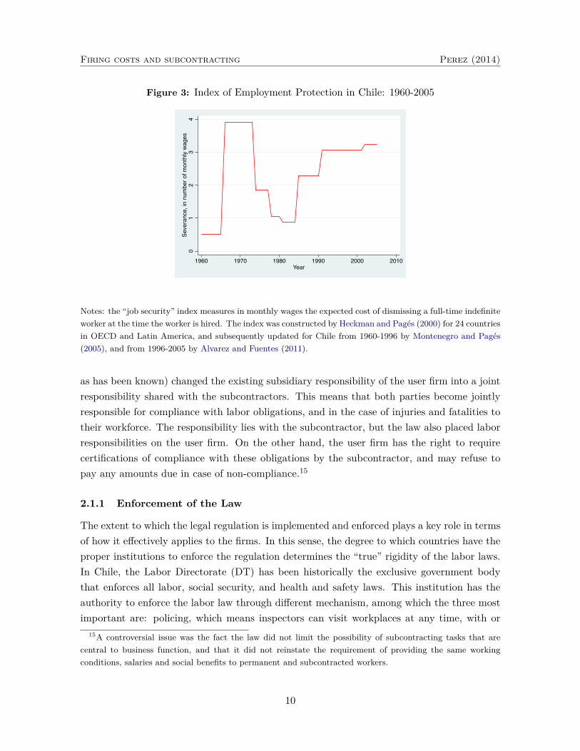
The extent of these reforms can be appreciated in Figure 3 by means of the “job security”index.12 This index measures in monthly wages the expected cost of dismissing a full-timeindefinite worker at the time of hiring, and it utilizes information on compulsory advancenotice periods, and compensations for dismissals. Given that the workers have the right tocontest dismissals, the index also includes a measure of the likelihood that a firm’s dismissalcause is considered unjust in court. After several years of low employment protection (late1970s and beginning 1980s), job security more than doubled in the mid-1980s to continuetrending up during the 1990s and 2000s. According to this index, firing costs in Chile areback to around 3 months’ wages.
In the meantime, regulation on subcontracted workers was kept isolated from the counter-reform process of the 1990s and 2000s. Towards the late-1970s the use of subcontractedworkers was completely liberalized, extending their use to any activity inside the firm, andeliminating all the restrictions preventing firms from subcontracting activities regarded ascentral to the business function, and periodic machine maintenance (a key component ofthe production process at that time).13 In addition, the requirement to provide the sameworking conditions, salaries and social benefits to permanent and subcontracted workers waseliminated. The law also prohibited subcontracted workers to join a union in the user firmwith the full-time workers under the rationale that their legal employer is the subcontractfirm.14
It was not until October 2006 that subcontracted work was regulated in Chile for the firsttime in large detail (Law No. 20, 123). The subcontracting law (or “anti-subcontracting law”
11See Edwards and Edwards (2000) for a complete description of the reforms to the labor market regulationfrom the early 1970s to the late 1990s. For a thorough description of the labor market regulation in place seeMicco and Repetto (2012).
12This index was constructed by Heckman and Pagés (2000) for 24 countries in OECD and Latin America,and subsequently updated for Chile from 1960-1996 by Montenegro and Pagés (2005) , and from 1996-2005 byAlvarez and Fuentes (2011).
13See Decree Law No. 2, 200 of 1978, and Decree Law No. 2, 759 of 1979.14The only protection that remained from the previous regulation was the subsidiary responsibility of the
user firms in relation to their subcontractors’ labor practices. This means the user firm is responsible forcompliance with these obligations only after it is not possible to sue the subcontract firm. Law No. 16, 757 of1968 regulated subcontracting before these modifications.
9
Firing costs and subcontracting Perez (2014)
Figure 3: Index of Employment Protection in Chile: 1960-2005
01
23
4Se
vera
nce,
in n
umbe
r of m
onth
ly w
ages
1960 1970 1980 1990 2000 2010Year
Notes: the “job security” index measures in monthly wages the expected cost of dismissing a full-time indefiniteworker at the time the worker is hired. The index was constructed by Heckman and Pagés (2000) for 24 countriesin OECD and Latin America, and subsequently updated for Chile from 1960-1996 by Montenegro and Pagés(2005), and from 1996-2005 by Alvarez and Fuentes (2011).
as has been known) changed the existing subsidiary responsibility of the user firm into a jointresponsibility shared with the subcontractors. This means that both parties become jointlyresponsible for compliance with labor obligations, and in the case of injuries and fatalities totheir workforce. The responsibility lies with the subcontractor, but the law also placed laborresponsibilities on the user firm. On the other hand, the user firm has the right to requirecertifications of compliance with these obligations by the subcontractor, and may refuse topay any amounts due in case of non-compliance.15
2.1.1 Enforcement of the Law
The extent to which the legal regulation is implemented and enforced plays a key role in termsof how it effectively applies to the firms. In this sense, the degree to which countries have theproper institutions to enforce the regulation determines the “true” rigidity of the labor laws.In Chile, the Labor Directorate (DT) has been historically the exclusive government bodythat enforces all labor, social security, and health and safety laws. This institution has theauthority to enforce the labor law through different mechanism, among which the three mostimportant are: policing, which means inspectors can visit workplaces at any time, with or
15A controversial issue was the fact the law did not limit the possibility of subcontracting tasks that arecentral to business function, and that it did not reinstate the requirement of providing the same workingconditions, salaries and social benefits to permanent and subcontracted workers.
10
Firing costs and subcontracting Perez (2014)
without a preceding charge made by an employee against the employer. They can also inspectphysical premises or business records. If inspectors find that an employer has violated a laborlaw, they can fine the employer, order the suspension of working activities, or even close theworkplace; administrative interpretation of the law (dictamen), which means they have thefaculty to determine the meaning and scope of the labor legislation; and file a complaint inthe labor courts in matters which it does not have authority (i.e. “unfair labor practices”,violations of “fundamental rights” or “disloyal” actions against employees.)
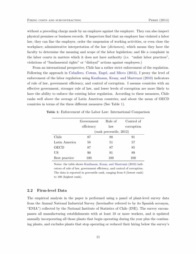
From an international perspective, Chile has a rather strict enforcement of the regulation.Following the approach in Caballero, Cowan, Engel, and Micco (2013), I proxy the level ofenforcement of the labor regulation using Kaufmann, Kraay, and Mastruzzi (2010) indicatorsof rule of law, government efficiency, and control of corruption. I assume countries with aneffective government, stronger rule of law, and lower levels of corruption are more likely tohave the ability to enforce the existing labor regulation. According to these measures, Chileranks well above the average of Latin American countries, and about the mean of OECDcountries in terms of the three different measures (See Table 1).
Table 1: Enforcement of the Labor Law: International Comparison
Government Rule of Control ofefficiency law corruption
(rank percentile, 2012)Chile 87 88 91Latin America 58 51 57OECD 87 87 85US 90 91 89Best practice 100 100 100
Notes: the table shows Kaufmann, Kraay, and Mastruzzi (2010) indi-cators of rule of law, government efficiency, and control of corruption.The data is reported in percentile rank, ranging from 0 (lowest rank)to 100 (highest rank).
2.2 Firm-level Data
The empirical analysis in the paper is performed using a panel of plant-level survey datafrom the Annual National Industrial Survey (hereinafter referred to by its Spanish acronym,“ENIA”) collected by the National Institute of Statistics of Chile (INE). The survey encom-passes all manufacturing establishments with at least 10 or more workers, and is updatedannually incorporating all those plants that begin operating during the year plus the continu-ing plants, and excludes plants that stop operating or reduced their hiring below the survey’s
11
Firing costs and subcontracting Perez (2014)
threshold. Each plant has a unique identification number which allows identification of entryand exit, and the computation of plant-level time-series.
The dataset is available for the period 1996 to 2011, but panel-data information for subcon-tracted work is only available from 2001 through 2007.16 Plant-year observations are droppedif permanent employment is either zero or missing. I also excluded the tobacco industry andpetroleum refineries from the analysis because they are organized as monopolies, operatingwith very few plants. This generates a sample of 10,906 plants and 69,938 observations withmean (median) employees of 72 (27). To ensure a reasonable sample size I run the estimationon the full panel, ignoring for now the specific industry to which the plants belong.
For each plant and year, the census collects detailed information on total number of em-ployees, separated by the contractual relationship between the plant and the employee. Em-ployers can hire workers under a permanent or full-time contract, or subcontract to a thirdparty the performance of a certain task or work with their own independent employees. Thesurvey also reports plants’ use of subcontracted workers in 6 different occupations: engineerand drafting services, blue-collar production, production assistant (i.e.machine maintenance,storage and transportation services), accounting services, blue-collar non-production (i.e. jan-itorial and secretarial services), and salesperson on commission.
2.3 Stylized Facts
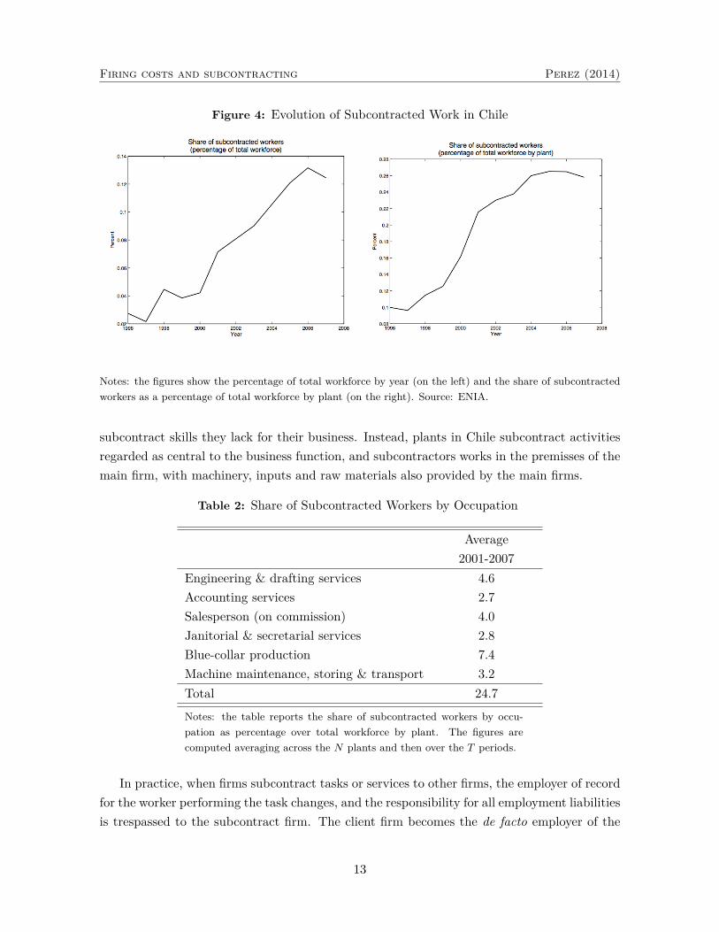
The effect of the employment protection gap between permanent and subcontracted workerscan be appreciated by looking at Figure 4, where I present the evolution of subcontractedworkers in Chile. Between 1996 and 2007, plants’ use of subcontracted workers skyrocketedin Chile; in 2007, 12 percent of the plants use subcontracted workers (up from 3 percent in1996), while among the plants that use subcontracted workers, around 3 out 10 workers perplant were subcontracted (up from 1 out of 10 in 1996).
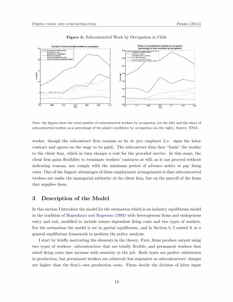
It is interesting to note that even when this modality of employment initially emergedin routine and low skilled occupations such as janitorial and security services, now it ispresent in key value-adding functions, such as logistics and accounting services, and high-skilled production-related occupations such as engineer and drafting services. Between 2001and 2007, plants subcontracted on average 25 workers out of every 100, where blue-collar pro-duction workers, and engineer and drafting services were the occupations that gathered thelargest number of subcontracted workers (See Table 2). During this period, these were also theoccupations that experienced the largest increase (see Figure 5). This echoes the fact that theform subcontracted work adopted in Chile is not the “specialized” one, where establishments
16Starting from 2008, the National Institute of Statistics ceased to release the plant unique identificationnumber necessary to match the plants abandoning the panel-structure. Before 2001 the classification to registersubcontracted worker was dramatically different so I also drop that information.
12
Firing costs and subcontracting Perez (2014)
Figure 4: Evolution of Subcontracted Work in Chile
Notes: the figures show the percentage of total workforce by year (on the left) and the share of subcontractedworkers as a percentage of total workforce by plant (on the right). Source: ENIA.
subcontract skills they lack for their business. Instead, plants in Chile subcontract activitiesregarded as central to the business function, and subcontractors works in the premisses of themain firm, with machinery, inputs and raw materials also provided by the main firms.
Table 2: Share of Subcontracted Workers by Occupation
Average2001-2007
Engineering & drafting services 4.6Accounting services 2.7Salesperson (on commission) 4.0Janitorial & secretarial services 2.8Blue-collar production 7.4Machine maintenance, storing & transport 3.2Total 24.7
Notes: the table reports the share of subcontracted workers by occu-pation as percentage over total workforce by plant. The figures arecomputed averaging across the N plants and then over the T periods.
In practice, when firms subcontract tasks or services to other firms, the employer of recordfor the worker performing the task changes, and the responsibility for all employment liabilitiesis trespassed to the subcontract firm. The client firm becomes the de facto employer of the
13
Firing costs and subcontracting Perez (2014)
Figure 5: Subcontracted Work by Occupation in Chile
Note: the figures show the total number of subcontracted workers by occupation (on the left) and the share ofsubcontracted workers as a percentage of the plant’s workforce by occupation (on the right). Source: ENIA.
worker, though the subcontract firm remains as its de jure employer (i.e. signs the laborcontract and agrees on the wage to be paid). The subcontract firm then “lends” the workerto the client firm, which in turn charges a cost for the provided service. In this sense, theclient firm gains flexibility to terminate workers’ contracts at will, as it can proceed withoutindicating reasons, nor comply with the minimum period of advance notice or pay firingcosts. One of the biggest advantages of these employment arrangements is that subcontractedworkers are under the managerial authority of the client firm, but on the payroll of the firmsthat supplies them.
3 Description of the Model
In this section I introduce the model for the estimation which is an industry equilibrium modelin the tradition of Hopenhayn and Rogerson (1993) with heterogenous firms and endogenousentry and exit, modified to include tenure dependent firing costs and two types of workers.For the estimation the model is set in partial equilibrium, and in Section 6, I embed it in ageneral equilibrium framework to perform the policy analysis.
I start by briefly motivating the elements in the theory. First, firms produce output usingtwo types of workers: subcontractors that are totally flexible, and permanent workers thatentail firing costs that increase with seniority in the job. Both types are perfect substitutesin production, but permanent workers are relatively less expensive as subcontractors’ chargesare higher than the firm’s own production costs. Firms decide the division of labor input
14
Firing costs and subcontracting Perez (2014)
between permanent and subcontracted labor as the optimal response to shocks.Second, there is ample evidence that employment adjustment at the plant level is charac-
terized by periods of sharp adjustment followed by long periods of inactivity, and the case ofChile is not any different.17 Thus, in the model I consider non-convex labor adjustment costs,in particular, piecewise linear adjustment costs, which can produce inaction and mimic thesefacts.
Third, I consider severance payments that increases with seniority in the job as the maincharacteristic of the employment protection regulation. In Chile, severance payments areequivalent to a month’s wage per year of service with a maximum of eleven months. Insteadof keeping track of the distribution of workers across tenure levels and increasing the dimensionof the problem, I assume permanent workers randomly get tenure, and that only workers withtenure are entitled to severance payments.
Finally, there is a continuum of ex ante identical potential entrants, and selection occursupon entry. Once firms enter the market they receive a random idiosyncratic productivitylevel, and they operate only if their first productivity draw is above the exit threshold. As thefirm’s productivity changes, it optimally chooses to grow, contract or exit the market. Sincethere are no aggregate shocks and the only source of uncertainty in the model is the firms’productivity, the distribution of firms over a size-productivity space is constant, and so allthe aggregate variables.
3.1 Firms and Technology
There is an industry composed of a continuum of firms that produce an homogenous good.Firms behave competitively taking prices in the output and labor markets as given. Each firmoperates a decreasing returns to scale, labor-only production function, using both permanentand subcontracted workers:
yt = f(nt, st, zt) = zt(nt + st)α (1)
where nt are the workers with a permanent contract, st the workers with subcontracts, α ∈(0, 1), and zt is the exogenous productivity that takes values in the finite set Z ≡ {z, ..., z}.The process for zt follows a First Order Markov Process with transition matrix Π(z, z′) andis i.i.d. across firms. This implies there is no uncertainty at the aggregate level.18
The two types of workers are perfect substitutes in production, but they differ in theirwages and firing costs:
17For evidence for the U.S., see Hamermesh (1989), and Caballero, Engel, and Haltiwanger (1997). Forevidence for other countries, see Varejão and Portugal (2007), complete
18These disturbances could also reflect shocks on the demand side, where firm produce differentiated goodsand the distribution of consumer tastes across this differentiated goods is stochastic over time. See Hopenhaynand Rogerson (1993) for a more detailed description of this alternative structure.
15

Firing costs and subcontracting Perez (2014)
i) Permanent workers are those with contracts of indefinite duration, and entail severancepay in case of dismissal. Permanent workers earn wage w. To avoid increasing thedimension of the problem and keeping track of the distribution of workers across tenurelevels, I assume permanent workers have (1 − λ) probability of getting tenure, and onlyworkers with tenure receive severance payments in case of dismissal. Workers with apermanent contract fired before tenure do not accrue severance pay.
Thus, workers with a permanent contract evolve:
nt = lt−1 + ot (2)
where lt−1 is the number of permanent workers with tenure employed last period, and otis the number of workers hired or fired in t. The law of motion for permanent workerswith tenure is:
lt ={lt−1 + (1− λ)ot, if ot > 0
lt−1 + ot, if ot ≤ 0.(3)
Since the optimal decision of current employment depends on the number of permanentworkers last period, lt−1 is a state variable for the firm.
Firing costs on permanent workers with tenure take a form similar to the work of Hopen-hayn and Rogerson (1993):
g(lt, lt−1) = max {0, τ (lt−1 − lt)} (4)
where τ is the fixed payment for every permanent worker laid-off. In principle, laboradjustment costs can consider the search, recruiting and training cost of hiring workers,but since the interest falls on the effect of severance payments I choose to ignore hiringcosts for now. This specification for labor adjustment costs imply the marginal costof changing employment is constant; hence, when the gains to changing the number ofworkers is small firms optimally choose not to adjust–marginal costs of adjustment donot go to zero as the size of the adjustment goes to zero, and there is no reason for thefirms to smooth adjustment. In this setting, firms’ labor adjustments are characterizedby episodes of sharp adjustment followed by periods of optimal inactivity.
ii) Subcontracted workers are those with temporary contracts subject to no costs for layingthem off. In turn, they are relatively more expensive than permanent workers as sub-contractors’ charges are higher than the firm’s own production costs. Firms can employsubcontracted workers for occasional or seasonal purposes, or jobs for absent, as well asjobs for carrying out a specific task or service for a determined period of time relatedto the production process. The subcontract firm legally employs the worker (signs the
16

Firing costs and subcontracting Perez (2014)
contract and pays the wage w), which in turn works on the premises of the user firmwho pays a fee per worker to the subcontract firm.19 Hence, subcontracted workers earnws = w(1+f), where f is the fee or wage premium on subcontracted labor. Provided thecost of subcontracting workers is small relative to the cost of adjusting in-house workers[1 − τ(1 − λ)], contracting out is an attractive alternative for the firms to cover peakdemand or productivity shocks.20
The operative profits of an active plant are given by
pyt − wnt − wsst − pcf − g(lt, lt−1) (5)
The timing of the model for incumbents is as follows:
1. Enter period t with last period’s shock zt−1 and permanent workers with tenure lt−1
2. Decide whether to exit. If the firm exits, pays the adjustment costs g(0, lt−1) for firingall workers from last period, and receives zero profits in all future periods avoiding topay cf .21
3. If the firm stays, it pays ptcf and receives this period’s shock, zt
4. Firm chooses labor demand and the number of workers to hire under each type ofcontract.
The timing for a potential entrant:
1. Pay the one-time entry cost ptce and then draw a productivity level zt from ν(z0) (whichis independent across firms)
2. Decide whether to stay in the industry. If the first productivity draw is above the exitthreshold the firm stays and produces as in 4 above.
19Subcontracted workers may be restricted by law or mutual agreements between firms and unions, so thatfirms are obliged to hire a certain amount of employees on a permanent basis. For example, it could be assumedthat the ratio between permanent and subcontracted workers can never fall below a minimum threshold ψ̄. Toremain faithful to the regulatory framework in Chile for the period under study, I assume no restrictions onsubcontracted labor and no hiring cost.
20The premium over subcontracted workers could also be justified on the basis of a compensation subcon-tracted workers demand to work on the firm considering their higher expected probability of losing the job.
21Fixed operating costs make the exit decision meaningful; plants exit to avoid paying the fixed cost insteadof simply waiting for a better realization of z and bearing an output of zero.
17
Firing costs and subcontracting Perez (2014)
3.2 Static Subproblem of the Firm
For any plant with z ∈ Z the optimal level of subcontracting solves the following staticproblem:
P (n, s, z) = maxs{pz(n+ s)α − n− wss− pcf}
st : s ≥ 0(6)
Note that the wage rate for permanent employees has been normalized w = 1, hence does notappear explicitly in the expression.
The solution implies that the optimal subcontracted labor choice is:
s(n, z) =
(αpzws
) 11−α − n, if αpznα−1 > ws
0, if αpznα−1 < ws(7)
Then, evaluating the profit function P (n, s, z) at the optimal subcontracted labor decisions(n, z), the operating profit of the plant R(n, z) is:
R(n, z) ≡ P (n, s(n, z), z) =
(
1−αα
) (αpzwαs
) 11−α + n(ws − 1)− pcf , if αpznα−1 > ws
pznα − n− pcf , if αpznα−1 < ws.(8)
3.3 Dynamic Optimization
Given that all uncertainty is idiosyncratic, I study a stationary equilibrium where pt = p. Inthis equilibrium, firm undergo change over time, with some of them growing or contracting,even exiting the market and others starting up. Since there are no aggregate shocks, despiteall these changes the distribution of firms over a size-productivity space is constant, and soall the aggregate variables.
3.3.1 Incumbent Firms
The dynamic programming problem of an incumbent plant that employed lt−1 permanentworkers last period, decided to remain in the industry this current period, and received thenew value for its shock zt is described by the Bellman equation:
V (lt−1, zt; p) = maxn
{R(nt, zt; p)− g(lt, lt−1) + βmax[Ezt+1V (lt, zt+1; p),−g(0, lt)]
}, (9)
subject to equation (2) and (3), and labor adjustment costs as defined in equation (4).Ezt+1 denotes the expectation of zt+1 conditional on the current value of productivity zt,
and β is the discount factor. The value V (lt−1, zt; p) is the expected discounted stream ofprofits from operating a plant with productivity zt and previous employment level lt−1. Giventhat the firm does not receive any new information between the current decision point and
18

Firing costs and subcontracting Perez (2014)
the time of the exit decision at the beginning of next period, it chooses now whether to exittomorrow. Conditional on this period’s employment decision, the firm stays if the exit cost,−g(0, lt), is larger than the expected value of staying, Ezt+1V (lt, zt+1; p).
In this framework, there are two decisions of an incumbent firm: i) optimal compositionof total employment nt = L(lt−1, zt; p), and st = S(nt, zt; p), and ii) optimal exit decision nextperiod xt+1 = X(lt, zt; p) ∈ {0, 1} with convention that X = 1 corresponds to exit and X = 0to stay.
3.3.2 Entry Decision
The decision whether to open a plant is also dynamic. It is profitable to open a new plant if:
V e(p) =∫V (0, z; p)dν(z) ≤ pce, (10)
where the value of of operating a new plant with productivity zt and no previous employment,lt−1 = 0, is:
V (0, zt; p) = maxn
{R(nt, zt; p) + βmax[Ezt+1V (lt, zt+1; p),−g(0, lt)]
}. (11)
subject to equation (3), (2) and labor adjustment costs as in equation (4).That is, new plants are open as long as the discounted expected profits from operating a
new plant are enough to cover the entry costs. In equilibrium with positive entry, the entryof new plants induces changes in the output price and the firm value until there are no gainsfrom entering this industry, and the constraint is satisfied with equality.
3.4 Stationary Distribution
In this model the state of an individual firm is fully described by (z, l), and the state of theindustry in turn is described by the distribution over the state variables for all firms. Let theincumbent firms at the beginning of the period be summarized by the measure µ(z, l) (afterthey have made their exit/stay decision and new realizations of z have arrived), and the massof firms that enter be equal to M .
The law of motion for the distribution of firms is given by
µ′(z, l) =∫z′
∫z[1−X(l, z; p)]F (z′/z)dµ(z, l) +
∫z′M ′dν(z) (12)
A stationary equilibrium is such that this distribution reproduces itself, i.e. µ′ = µ.The equilibrium distribution of productivity and permanent employment is determined by
the productivity of entrants, the stochastic process of productivity, the extent of selection,and the number of entrants. Once the distribution of the state variables has been determinedit is possible to compute all aggregate variables.
19
Firing costs and subcontracting Perez (2014)
Total supply in the industry is:
Qs(µ,M ; p) =∫z∗f(L(l, z; p), S(n, z; p), z)dµ(z, l) +M
∫z∗f(L(0, z; p), S(n, z; p), z)dν(z).
(13)Aggregate demand for this industry follows a standard representation: Qd = D(P )
3.5 Definition of Equilibrium
A stationary industry equilibrium with positive entry and exit is a set of value functionsand decision rules, a price p∗, a stationary distribution of firms µ∗, and a mass of entrantsM∗ such that:
1. Given prices, the value functions of the firms and the policy functions are consistentwith firms optimization
2. Markets clear: p∗ = D(Q∗) and Q∗ = Qs(µ∗, p∗, w∗)
3. There is an invariant distribution over firms: µ∗ = T (µ∗,M∗; p∗)
4. The free entry condition is satisfied: V e(p∗) = p∗ce
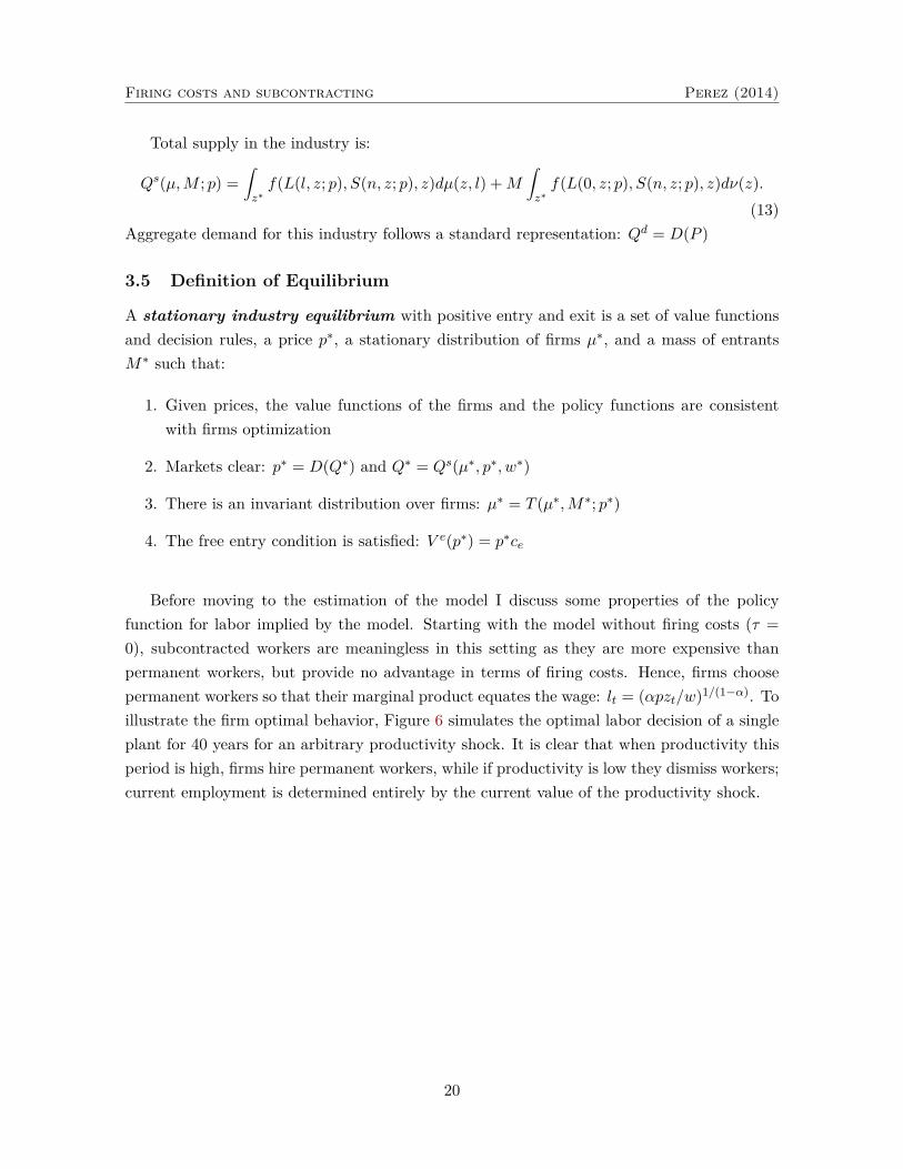
Before moving to the estimation of the model I discuss some properties of the policyfunction for labor implied by the model. Starting with the model without firing costs (τ =0), subcontracted workers are meaningless in this setting as they are more expensive thanpermanent workers, but provide no advantage in terms of firing costs. Hence, firms choosepermanent workers so that their marginal product equates the wage: lt = (αpzt/w)1/(1−α). Toillustrate the firm optimal behavior, Figure 6 simulates the optimal labor decision of a singleplant for 40 years for an arbitrary productivity shock. It is clear that when productivity thisperiod is high, firms hire permanent workers, while if productivity is low they dismiss workers;current employment is determined entirely by the current value of the productivity shock.
20
Firing costs and subcontracting Perez (2014)
Figure 6: Optimal Labor Decision: Model Without Firing Costs
Notes: the figure shows the optimal labor decision of a single plant for 40 years for an arbitrary productivityshock when permanent workers do not entail firing costs. The parameters are given in Table 6 (Panel B, row1, model with quick tenure) for τ = 0.
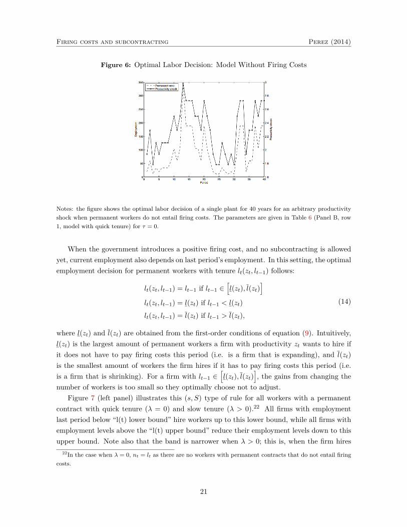
When the government introduces a positive firing cost, and no subcontracting is allowedyet, current employment also depends on last period’s employment. In this setting, the optimalemployment decision for permanent workers with tenure lt(zt, lt−1) follows:
lt(zt, lt−1) = lt−1 if lt−1 ∈[l(zt), l(zt)
]lt(zt, lt−1) = l(zt) if lt−1 < l(zt)
lt(zt, lt−1) = l(zt) if lt−1 > l(zt),
(14)
where l(zt) and l(zt) are obtained from the first-order conditions of equation (9). Intuitively,l(zt) is the largest amount of permanent workers a firm with productivity zt wants to hire ifit does not have to pay firing costs this period (i.e. is a firm that is expanding), and l(zt)is the smallest amount of workers the firm hires if it has to pay firing costs this period (i.e.is a firm that is shrinking). For a firm with lt−1 ∈
[l(zt), l(zt)
], the gains from changing the
number of workers is too small so they optimally choose not to adjust.Figure 7 (left panel) illustrates this (s, S) type of rule for all workers with a permanent
contract with quick tenure (λ = 0) and slow tenure (λ > 0).22 All firms with employmentlast period below “l(t) lower bound” hire workers up to this lower bound, while all firms withemployment levels above the “l(t) upper bound” reduce their employment levels down to thisupper bound. Note also that the band is narrower when λ > 0; this is, when the firm hires
22In the case when λ = 0, nt = lt as there are no workers with permanent contracts that do not entail firingcosts.
21
Firing costs and subcontracting Perez (2014)
permanent workers knowing that with probability (1−λ) they will actually get tenure.23 Thesame figure, on the right, simulates the optimal labor decision of a single plant for 40 years foran arbitrary productivity shock with quick tenure (λ = 0) and slow tenure (λ > 0). Consistentwith the policy function, firms hire permanent workers only if the productivity shock is largeenough, and we observe periods of sharp adjustment followed by long periods of inactivity.When λ > 0, the fact that not all workers get tenure gives the firm some flexibility to adjustemployment to changes in productivity more often. Employment becomes more volatile inthis case, and firms can use resources more efficiently.
Figure 7: Optimal Labor Decision: Model With Firing Costs and No Subcontracting
Notes: the figures illustrate the policy function for all workers with a permanent contract (on the left), andthe optimal labor decision of a single plant for 40 years for an arbitrary productivity shock when permanentworkers entail firing costs (on the right). Two cases are plotted: quick tenure (λ = 0) and slow tenure (λ > 0).The parameters are given in Table 6 (Panel B, row 3, model with slow tenure).
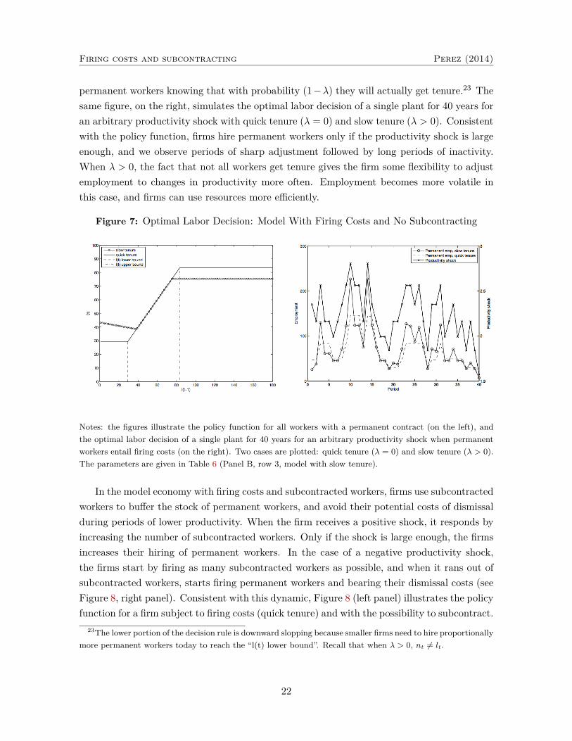
In the model economy with firing costs and subcontracted workers, firms use subcontractedworkers to buffer the stock of permanent workers, and avoid their potential costs of dismissalduring periods of lower productivity. When the firm receives a positive shock, it responds byincreasing the number of subcontracted workers. Only if the shock is large enough, the firmsincreases their hiring of permanent workers. In the case of a negative productivity shock,the firms start by firing as many subcontracted workers as possible, and when it rans out ofsubcontracted workers, starts firing permanent workers and bearing their dismissal costs (seeFigure 8, right panel). Consistent with this dynamic, Figure 8 (left panel) illustrates the policyfunction for a firm subject to firing costs (quick tenure) and with the possibility to subcontract.
23The lower portion of the decision rule is downward slopping because smaller firms need to hire proportionallymore permanent workers today to reach the “l(t) lower bound”. Recall that when λ > 0, nt 6= lt.
22
Firing costs and subcontracting Perez (2014)
When firms can subcontract, the “inaction band” narrows with respect to the case withoutsubcontracting (compare the solid line labeled Total with the dashed line labeled Permanentno subcontracting) coming closer to reach the optimal level of employment without distortions.Hence, the extent to which resources are not allocated efficiently decreases. Also, the increasein employment up to the “lower bound”, is attained by a combined increase of subcontractedand permanent workers. As explained before, firms begin subcontracting workers, and only ifthe productivity shock is large enough they increase their hiring of permanent workers.
Figure 8: Optimal Labor Decision: Model With Firing Costs and Subcontracting
Notes: the figures illustrate the policy function for all workers with a permanent contract and quick tenure (onthe left), and the optimal labor decision of a single plant for 40 years for an arbitrary productivity shock whenpermanent workers entail firing costs and plants can subcontract (on the right). The parameters are given inTable 5 (Panel B, row 3, model with slow tenure).
3.6 Solution Method
The model has no closed-form solution hence it is solved numerically. In appendix A I presenta detailed characterization of the computation method used to solve the model.
The model period is one year. I assume firm’s idiosyncratic shocks follow an AR(1) processof the form:
log zt = µ+ ρ log zt−1 + εt (15)
where µ is a constant, ρ the persistence of the shocks, and εt is a random variable withstandard normal distribution. I approximate the distribution of the idiosyncratic shocksusing the quadrature-based method developed in Rouwenhorst (1995), which has been shownto be more reliable in approximating highly persistent processes, and choose the number of
23
Firing costs and subcontracting Perez (2014)
grid points gz = 30. The initial distribution ν(z0) is chosen to be the stationary distributionof the z process which matches well the size distribution of the firms age 0-1 years in the data.
Industry demand is given by a decreasing function. For simplicity, take the followingiso-elastic functional form:
p = Q− 1η , (16)
where p is output price, Q is the industry output, and η > 0 is the price elasticity of demandelasticity.
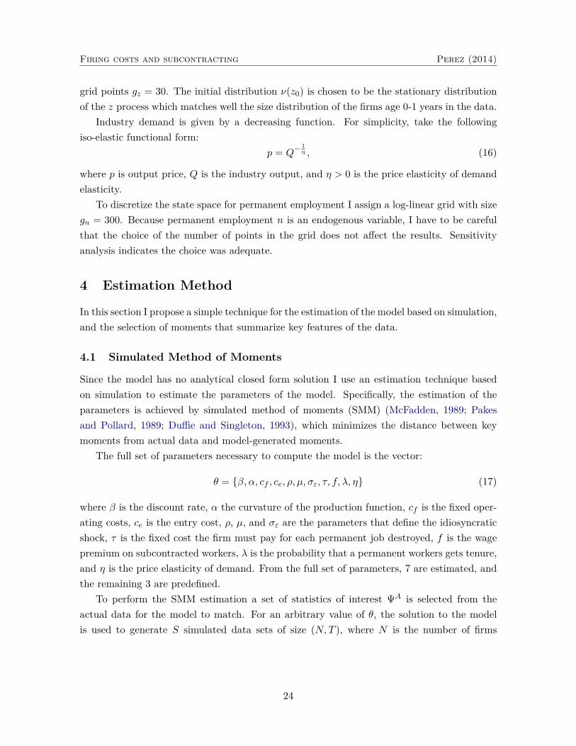
To discretize the state space for permanent employment I assign a log-linear grid with sizegn = 300. Because permanent employment n is an endogenous variable, I have to be carefulthat the choice of the number of points in the grid does not affect the results. Sensitivityanalysis indicates the choice was adequate.
4 Estimation Method
In this section I propose a simple technique for the estimation of the model based on simulation,and the selection of moments that summarize key features of the data.
4.1 Simulated Method of Moments
Since the model has no analytical closed form solution I use an estimation technique basedon simulation to estimate the parameters of the model. Specifically, the estimation of theparameters is achieved by simulated method of moments (SMM) (McFadden, 1989; Pakesand Pollard, 1989; Duffie and Singleton, 1993), which minimizes the distance between keymoments from actual data and model-generated moments.
The full set of parameters necessary to compute the model is the vector:
θ = {β, α, cf , ce, ρ, µ, σε, τ, f, λ, η} (17)
where β is the discount rate, α the curvature of the production function, cf is the fixed oper-ating costs, ce is the entry cost, ρ, µ, and σε are the parameters that define the idiosyncraticshock, τ is the fixed cost the firm must pay for each permanent job destroyed, f is the wagepremium on subcontracted workers, λ is the probability that a permanent workers gets tenure,and η is the price elasticity of demand. From the full set of parameters, 7 are estimated, andthe remaining 3 are predefined.
To perform the SMM estimation a set of statistics of interest ΨA is selected from theactual data for the model to match. For an arbitrary value of θ, the solution to the modelis used to generate S simulated data sets of size (N,T ), where N is the number of firms
24

Firing costs and subcontracting Perez (2014)
and T is the number of periods.24 The simulated moments ΨS(θ) are computed on eachdata set and then averaged out to compute the minimizing criterion function: Γ(θ) = [ΨA −1S
∑Ss=1 ΨS(θ)]′ W [ΨA − 1
S
∑Ss=1 ΨS(θ)]. I use the same random draw for the productivity
shock throughout each simulation.The parameter estimate θ̂ is obtained by searching over the parameter space to minimize
the (weighted) distance between the moments implied by the model and those computed fromthe data:
θ̂ = arg minθ∈Θ
[ΨA − 1S
S∑s=1
ΨS(θ)]′ W [ΨA − 1S
S∑s=1
ΨS(θ)], (18)
where W is a weighting matrix and Θ the estimated parameters space. θ̂ is consistent for anypositive-definite weighting matrix (e.g. identity matrix) but the smallest asymptotic varianceis obtained when the weighting matrix equals the inverse of the covariance matrix of the datamoments, V . In this case, I use W = diag(V −1) (diagonal elements equal to those of V andoff-diagonal elements equal zero) because it has better small sample properties (see Altonjiand Segal (1996)). V is calculated by bootstrap with replacement on the actual data.25 Tominimize the function I use Nelder-Mead simplex algorithm starting from 1, 000 differentinitial guesses to ensure the solution converges to the global minima.
To generate the standard errors of the parameter point estimates, I compute the numericalderivatives of the simulated moments with respect to the parameters and using the standardSMM formula compute the asymptotic variance:26
SE(θ̂) =[(J ′WJ)−1
]1/2, (19)
where J = E(∂ΨS(θ)/∂θ) of dimension p (#moments) × q (#parameters). Given the un-derlying discontinuities of the value functions, I follow the methodology in Bloom (2009) tocompute the numerical derivatives. I calculate the numerical derivative as f ′(x) = f(x+ε)−f(x)
ε
for an ε of ±5%, ±2.5%, and ±1% of the midpoint of the parameter space. Then, I simplycompute the median value of these derivatives.
4.2 Predefined Paramaters
The predefined parameters are shown in Table 3. Parameter β is set to be equal to 0.965,which is equivalent to annual real interest rate over the period of study of 3.62%. Becausethe curvature of the production function is difficult to identify in the data, I also set its valuea priori. α not only captures the labor share in the total revenue, but also decreasing returns
24I set N=5,000 and T=200 which implies the number of firms in the simulation is approximately 10 timeslarger than in the data. I discard the first 50 periods of simulated data to start from the stationary distribution.
25To preserve the original time-series structure of the data to conduct inference I resample firm’s completetime-series.
26See Gouriéroux and Monfort (1997).
25

Firing costs and subcontracting Perez (2014)
to scale and the elasticity of demand of firms’ output. If capital is flexible, the elasticity ofdemand is infinite, and there is constant return to scale, then α should equal one. Relaxingany of these assumptions leads to an α < 1 (See Roys and Gourio (2013)). I choose α equalto 0.85 so that for η = 4 the labor share is consistent with previous estimations for Chile.27
The value of ce is chosen so that the free-entry condition (10) holds under p = 1, and thewage rate of permanent workers is normalized to 1.
Table 3: Predefined Parameters in the Model
Parameter Description Valueβ Discount rate 0.965α Curvature production function 0.85η Price elasticity of industry demand 4
4.3 Selection of Moments
The choice of moments is guided by their “informativeness” regarding the underlying structuralparameters to be estimated. In particular, the exact choice of moments is directed by acombination of cross-sectional industry characteristics and time-series employment dynamics.Heuristically, a moment is informative about a certain parameter if that moment varies whenthe parameter varies. Table 4 shows the elasticities of model moments with respect to themodel parameters.
To pin down the fixed operating costs parameter I attempt to match the exit rate, theaverage firm size, and the firm size and employment distribution. An increase in fixed op-erating costs cf increases the minimum level of productivity needed for incumbents firms tosurvive. This, in turn, intensifies market selection, and decreases entry barriers, resulting ina distribution of surviving firms with a larger proportion of high productivity establishments(see column (1) in Table 4). These same moments are also informative about the mean µ,persistence ρ and volatility σε of the productivity process. An increase in µ or the volatility σε,increase the exit rate, and decrease the average mean size of firms shifting the size distributiontowards more small firms. Instead, the persistence parameter ρ increase the average size offirms and decreases the exit rate, shifting the size distribution towards more large plants (seecolumns (3), (4) and (5) in Table 4).
To study employment dynamics I use a modified definition of employment growth fol-lowing Davis and Haltiwanger (1992): git = (xit − xit−1)/(0.5 ∗ (xit + xit−1)), where xit is
27Estimations for the labor share parameter in Chile range from 0.53 − 0.6. These estimates are somehowlower than those for the US economy because of a larger participation of natural resources in the GDP, and alow stock of human capital.
26

Firing costs and subcontracting Perez (2014)
the number of employees (subcontracted or permanent) in plant i at time t. This growthmeasure is symmetric about zero, and lies in the close interval [−2, 2] with deaths (births)corresponding to the left (right) endpoints. The conventional growth rate measure (changein employment divided by lagged employment) does not allow for an integrated treatment of“exits” and “entries”. However, a significant fraction of the adjustments in subcontracted em-ployment corresponds to these cases so this information cannot be ignored; this is, plants thathire subcontracted workers this period after not having employed them the previous period(“entry”), and plants that cease to subcontract today after having hired subcontracted work-ers the previous period (“exit”), even when they still remain in operation. For consistency,growth in both types of employment is computed using this measure.
A key feature of the employment data is that permanent employment fluctuations aresmoother and less frequent than fluctuations in subcontracted workers. It is transparent thatthe distribution of permanent employment growth rates is more peaked and with heavier tails,implying that there is a higher proportion of extreme events (even when sharp adjustments arestill rare). Instead, the distribution of subcontracted employment growth rates indicates moresmooth and persistent adjustment. Further, the permanent employment growth distributionhas a considerable amount of mass around 0 (see Figure 2 in Section 1). I select moments thatdescribe these features of the distribution of both permanent and subcontracted growth rates;this is, volatility and kurtosis of the distribution, and inaction rate of permanent employment.
To pin down λ, τ and f I attempt to match the volatility and kurtosis of permanent andsubcontracted employment growth, and the inaction rate of permanent employment growth.When τ increases, firms use more subcontracted workers as they rely more on these workers tobuffer permanent employment from economic fluctuations. As a consequence, the volatility ofpermanent employment decreases, the inaction rate of employment growth increases, and thekurtosis increases (see column (7) in Table 4). In turn, when λ decreases (the probability ofgetting tenure for permanent workers increase), firms have to rely more on permanent workersincreasing (decreasing) the volatility (kurtosis) of permanent workers growth rate (see column(2) in Table 4). Similarly, when the premium on subcontracted work f increases the volatilityof subcontracted workers increases as firms use subcontract workers more infrequently (seecolumn (6) in Table 4). The variance of permanent employment growth rate is informativeabout the mean, persistence and volatility of the productivity process.
Lastly, to complete the selection of moments I choose to match the proportion of subcon-tracted workers over the firm workforce as this is informative about the fixed lay-off cost τ(i.e. higher firing costs more subcontracting by the firms), the premium over subcontractedworkers f (i.e. higher the premium less subcontracting), and λ (i.e. an decrease in the prob-ability of getting tenure, decreases the adjustment costs of permanent employment, and theadvantage of using subcontracted workers). Note also that the share of subcontracting isinformative about the persistence (i.e. more persistent the risk decreases and firms use less
27

Firing costs and subcontracting Perez (2014)
subcontracted workers), and the volatility of the productivity process (i.e. an increase in thevolatility increases the risk and firms rely more on subcontracted workers).
Table 4: Sensitivity of Model Moments to Parameters
(1) (2) (3) (4) (5) (6) (7)Moments cf λ ρ µ σε f τ
Average firm size 1.094 0.005 1.963 -0.201 -0.388 -0.207 -0.045Exit rate 1.502 0.005 -7.903 0.736 1.550 0.003 -0.006Fraction of plants in each bin:10-19 emp. -1.225 -0.004 -2.240 0.073 0.253 -0.160 0.01720-99 emp. 0.903 0.004 2.165 -0.055 -0.229 0.131 -0.006100-499 emp. 1.219 -0.001 1.113 -0.029 -0.140 0.002 -0.004500+ emp. 1.331 -0.001 0.933 -0.084 -0.166 -0.005 -0.001Share of employment in each bin:10-19 emp. -1.944 -0.033 -1.125 0.077 0.110 0.085 0.04120-99 emp. -0.127 0.029 1.276 -0.037 -0.218 0.216 -0.106100-499 emp. 0.151 -0.008 -0.329 0.086 0.136 -0.064 0.032500+ emp. 0.296 -0.008 -0.149 -0.001 0.051 -0.072 0.056Volatility gl 0.838 0.419 -4.293 0.378 0.842 0.056 -0.054Volatility gs -0.456 0.117 -0.808 0.038 0.335 0.349 -0.330Kurtosis gl -0.952 -0.241 5.196 -0.476 -1.095 -0.200 0.224Kurtosis gs 0.182 -0.057 1.617 -0.296 -0.553 -0.148 0.140Share of subcontracting 0.406 -0.120 -4.916 0.304 0.796 -0.336 0.365Inaction rate gl -0.302 0.000 1.648 -0.348 -0.464 -0.086 0.155
Notes: this table presents elasticities of model moments with respect to the model parameters. To calculatethe elasticities the numerical derivatives of the model moments with respect to the parameters are multipliedby the ratio of the baseline parameters to the baseline moments. The numerical derivative is the medianvalue of the numerical derivatives f ′(x) = (f(x + ε) − f(x))/ε for an ε of ±5%, ±2.5%, and ±1% of themidpoint of the parameter space.
5 Empirical Results
In this section I present the estimates from the simulated method of moment. In Table 5, thecolumn labeled Data reports the actual moments from ENIA, and next to it the associatedstandard errors. These show that permanent employment fluctuations are smoother and lessfrequent than fluctuations in subcontracted workers (the volatility of employment growth rate
28
Firing costs and subcontracting Perez (2014)
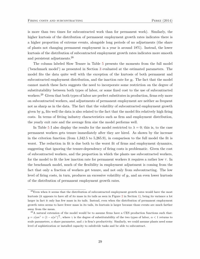
is more than two times for subcontracted work than for permanent work). Similarly, thehigher kurtosis of the distribution of permanent employment growth rates indicates there isa higher proportion of extreme events, alongside long periods of no adjustments (the shareof plants not changing permanent employment in a year is around 18%). Instead, the lowerkurtosis of the distribution of subcontracted employment growth rates indicates more smoothand persistent adjustments.28
The column labeled Slow Tenure in Table 5 presents the moments from the full model(’benchmark model’) as presented in Section 3 evaluated at the estimated parameters. Themodel fits the data quite well with the exception of the kurtosis of both permanent andsubcontracted employment distribution, and the inaction rate for gl. The fact that the modelcannot match these facts suggests the need to incorporate some restriction on the degree ofsubstitutability between both types of labor, or some fixed cost to the use of subcontractedworkers.29 Given that both types of labor are perfect substitutes in production, firms rely moreon subcontracted workers, and adjustments of permanent employment are neither as frequentnot as sharp as in the data. The fact that the volatility of subcontracted employment growthgiven by gs fits well the data is also related to the fact that the model fits relatively high firingcosts. In terms of fitting industry characteristics such as firm and employment distribution,the yearly exit rate and the average firm size the model performs well.
In Table 5 I also display the results for the model restricted to λ = 0; this is, to the casepermanent workers gets tenure immediately after they are hired. As shown by the increasein the criterion function (from 1,342.5 to 5,265.9), in comparison to the full model the fit isworst. The reduction in fit is due both to the worst fit of firms and employment dynamics,suggesting that ignoring the tenure-dependency of firing costs is problematic. Given the costof subcontracted workers, and the proportion in which the plants use subcontracted workers,for the model to fit the low inaction rate for permanent workers it requires a rather low τ . Inthe benchmark model, much of the flexibility in employment adjustment is coming from thefact that only a fraction of workers get tenure, and not only from subcontracting. The lowlevel of firing costs, in turn, produces an excessive volatility of gl, and an even lower kurtosisof the distribution of permanent employment growth rates.
28Even when it seems that the distribution of subcontracted employment growth rates would have the mostkurtosis (it appears to have all of its mass in its tails as seen in Figure 2 in Section 1), being its variance a lotlarger in fact it only has few mass in its tails. Instead, even when the distribution of permanent employmentgrowth rates seems to have fewer mass in its tails, its kurtosis is larger because those events are much fartheraway from the mean.
29A natural extension of the model would be to assume firms have a CES production functions such that:y = z(anγ + (1− a)sγ)
αγ , where γ is the degree of substitutability of the two types of labor, α < 1 returns to
scale parameters, a share parameter, and z is firm’s productivity. Similarly, we could assume plants need somelevel of sophistication or installed capacity to subdivide tasks and be able to subcontract.
29

Firing costs and subcontracting Perez (2014)
Table 5: Simulated Moments Estimations for the Full Model
Panel A: Moments
Moments Data S.E. Simulated MomentsSlow Tenure Quick Tenure
(λ > 0) (λ = 0)Average firm size 71.95 1.8782 71.53 64.79Exit rate 0.091 0.0012 0.098 0.135Fraction of plants in each bin:10-19 employees 0.386 0.0049 0.398 0.45720-99 employees 0.447 0.0049 0.436 0.407100-499 employees 0.145 0.0038 0.148 0.121More than 500 employees 0.022 0.0016 0.018 0.016Share of employment in each bin:10-19 employees 0.064 0.0021 0.062 0.08420-99 employees 0.260 0.0081 0.264 0.296100-499 employees 0.417 0.0118 0.398 0.371More than 500 employees 0.260 0.0173 0.275 0.249Volatility gl 0.688 0.0160 0.781 0.818Volatility gs 2.161 0.0618 2.118 2.519Kurtosis gl 5.144 0.0606 3.141 2.689Kurtosis gs 1.973 0.0273 1.645 1.704Inaction rate gl 0.181 0.0026 0.231 0.175Share of subcontracting 0.247 0.0053 0.253 0.278Criterion, Γ(θ) 1,342.52 5,265.9
Panel B: Parameter Estimates
cf λ ρ µ σε f τ
Quick tenure 4.807 - 0.903 0.023 0.139 0.095 0.160(λ = 0) (0.0353) - (0.0197) (0.0047) (0.0198) (0.0027) (0.0421)Slow tenure 6.384 0.758 0.913 0.029 0.129 0.101 0.593
(0.0403) (0.0284) (0.0113) (0.0025) (0.0121) (0.0025) (0.0284)
Notes: Panel A reports the targeted moments and their corresponding standard errors, and the simulatedmoments evaluated at the estimated parameters. The bottom table reports the parameters’ point estimatesand their standard errors in parenthesis.
30
Firing costs and subcontracting Perez (2014)
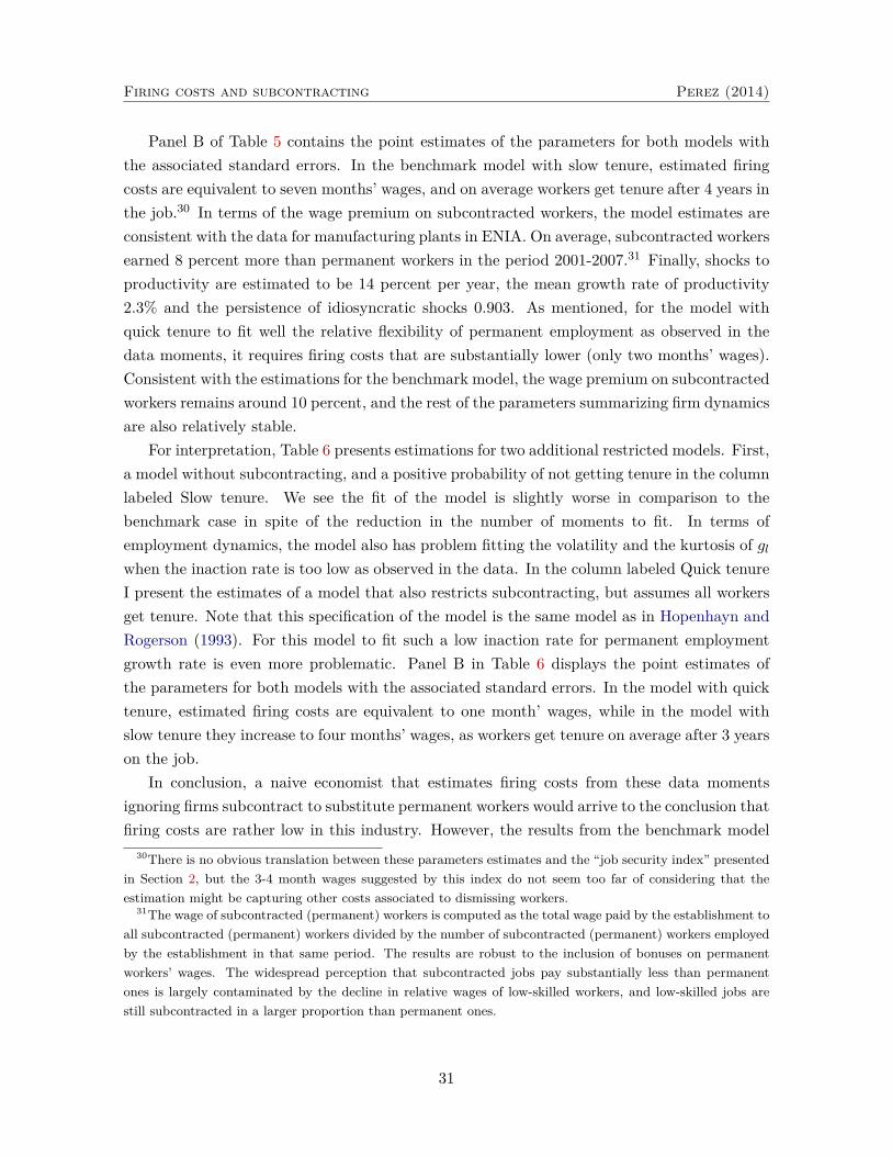
Panel B of Table 5 contains the point estimates of the parameters for both models withthe associated standard errors. In the benchmark model with slow tenure, estimated firingcosts are equivalent to seven months’ wages, and on average workers get tenure after 4 years inthe job.30 In terms of the wage premium on subcontracted workers, the model estimates areconsistent with the data for manufacturing plants in ENIA. On average, subcontracted workersearned 8 percent more than permanent workers in the period 2001-2007.31 Finally, shocks toproductivity are estimated to be 14 percent per year, the mean growth rate of productivity2.3% and the persistence of idiosyncratic shocks 0.903. As mentioned, for the model withquick tenure to fit well the relative flexibility of permanent employment as observed in thedata moments, it requires firing costs that are substantially lower (only two months’ wages).Consistent with the estimations for the benchmark model, the wage premium on subcontractedworkers remains around 10 percent, and the rest of the parameters summarizing firm dynamicsare also relatively stable.
For interpretation, Table 6 presents estimations for two additional restricted models. First,a model without subcontracting, and a positive probability of not getting tenure in the columnlabeled Slow tenure. We see the fit of the model is slightly worse in comparison to thebenchmark case in spite of the reduction in the number of moments to fit. In terms ofemployment dynamics, the model also has problem fitting the volatility and the kurtosis of glwhen the inaction rate is too low as observed in the data. In the column labeled Quick tenureI present the estimates of a model that also restricts subcontracting, but assumes all workersget tenure. Note that this specification of the model is the same model as in Hopenhayn andRogerson (1993). For this model to fit such a low inaction rate for permanent employmentgrowth rate is even more problematic. Panel B in Table 6 displays the point estimates ofthe parameters for both models with the associated standard errors. In the model with quicktenure, estimated firing costs are equivalent to one month’ wages, while in the model withslow tenure they increase to four months’ wages, as workers get tenure on average after 3 yearson the job.
In conclusion, a naive economist that estimates firing costs from these data momentsignoring firms subcontract to substitute permanent workers would arrive to the conclusion thatfiring costs are rather low in this industry. However, the results from the benchmark model
30There is no obvious translation between these parameters estimates and the “job security index” presentedin Section 2, but the 3-4 month wages suggested by this index do not seem too far of considering that theestimation might be capturing other costs associated to dismissing workers.
31The wage of subcontracted (permanent) workers is computed as the total wage paid by the establishment toall subcontracted (permanent) workers divided by the number of subcontracted (permanent) workers employedby the establishment in that same period. The results are robust to the inclusion of bonuses on permanentworkers’ wages. The widespread perception that subcontracted jobs pay substantially less than permanentones is largely contaminated by the decline in relative wages of low-skilled workers, and low-skilled jobs arestill subcontracted in a larger proportion than permanent ones.
31
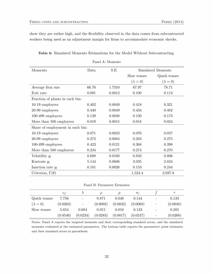
Firing costs and subcontracting Perez (2014)
show they are rather high, and the flexibility observed in the data comes from subcontractedworkers being used as an adjustment margin for firms to accommodate economic shocks.
Table 6: Simulated Moments Estimations for the Model Without Subcontracting
Panel A: Moments
Moments Data S.E. Simulated MomentsSlow tenure Quick tenure(λ > 0) (λ = 0)
Average firm size 66.76 1.7310 67.97 78.71Exit rate 0.091 0.0012 0.100 0.113Fraction of plants in each bin:10-19 employees 0.402 0.0049 0.418 0.32120-99 employees 0.440 0.0049 0.434 0.482100-499 employees 0.139 0.0038 0.130 0.173More than 500 employees 0.019 0.0015 0.018 0.024Share of employment in each bin:10-19 employees 0.071 0.0023 0.076 0.05720-99 employees 0.272 0.0084 0.283 0.275100-499 employees 0.423 0.0121 0.368 0.398More than 500 employees 0.234 0.0177 0.274 0.270Volatility gl 0.688 0.0160 0.833 0.806Kurtosis gl 5.144 0.0606 3.035 2.834Inaction rate gl 0.181 0.0026 0.153 0.244Criterion, Γ(θ) 1,524.4 2,937.9
Panel B: Parameter Estimates
cf λ ρ µ σε f τ
Quick tenure 7.756 - 0.871 0.048 0.144 - 0.133(λ = 0) (0.0263) - (0.0092) (0.0032) (0.0068) - (0.0048)Slow tenure 5.654 0.684 0.915 0.016 0.133 - 0.285
(0.0546) (0.0234) (0.0283) (0.0017) (0.0247) - (0.0268)
Notes: Panel A reports the targeted moments and their corresponding standard errors, and the simulatedmoments evaluated at the estimated parameters. The bottom table reports the parameters’ point estimatesand their standard errors in parenthesis.
32

Firing costs and subcontracting Perez (2014)
6 Policy Implications
In this section, I extend the partial-equilibrium model to a general equilibrium framework,and using the parameters’ estimates I carry out several policy analysis. I use the estimationsfor the four models to analyze the implementation of two alternative labor market reforms:first, the elimination of subcontracted workers and, second, the reduction of firing costs to zerowhen suitable. This experiment is relevant in light of the debate that pits workers’ demandsto limit the use of subcontracting as a way to improve their working conditions, with those ofthe business community that advocate a reduction in firing costs. Finally, it is important toclarify that the model is not appropriate for welfare analysis as it only considers a frictionlesseconomy in which firing costs have no potential benefits, but to distort the job reallocationprocess. The equilibrium allocation without government intervention is Pareto optimal, hencethere is no space for improvement coming from firing costs.32
6.1 General Equilibrium Model
The economy is populated by a continuum of identical two member households: workers thatsupply labor under a permanent contract and subcontracted workers. Each household haspreferences defined over consumption and labor supply given by:
∞∑t=1
βt[log(ct)−Bn1+φt
1 + φ], (20)
where ct > 0 is total consumption, and nt is labor effort. Parameters B and φ representpreferences for leisure, and the inverse of the Frisch elasticity of labor supply, respectively.Households take all of the income from all of the workers, and allocate it to the individualswithin the household. Also, they allocate total hours worked independent of which workersperforms the effort.
The output price is normalized to one, and the households supplies labor to the marketat the wage w = −un/uc = Bcnφ. As before, both members of the household are perfectsubstitutes in production, but permanent workers are relatively less expensive as subcon-tractors’ charges are higher than the firm’s own production costs. Subcontract firms incurin a real cost for “creating” subcontracted workers, and the premium they charge to themain firm per worker is just enough to cover the real cost c so that their profits are zero:π(st) = (wst − c)st = 0. The cost for firms to subcontract a worker is wst = wt(1 + f). Iconsider a stationary equilibrium, so all prices and aggregates in the economy are constant,and household maximization implies the interest rate satisfies 1/(1 + r) = β.
32See, for example, Alvarez and Veracierto (2001) and Alonso-Borrego, Fernández-Villaverde, and Galdón-Sánchez (2004) who analyze the impact of firing costs in an economy with imperfect insurance markets andsearch frictions.
33
Firing costs and subcontracting Perez (2014)
An individual firm that employed lt−1 permanent workers last period and draws a produc-tivity shock zt this period has expected adjustment costs given by:
r(lt−1, zt;w) = [1−X(lt, zt;w)]∫g(nt+1, lt)dF (zt+1, zt) +X(lt, zt;w)g(0, lt), (21)
where nt+1 = L(lt, zt+1;w). Integration yields aggregate adjustment costs given byR(µ,M ;w).I assume proceeds from the regulation are rebated uniformly to all households as a lump-sumpayment to households by the government. In fact, severance payments make up for thelargest part of firing costs in Chile, and are paid entirely to the workers when they are fired.Aggregate adjustment costs do not appear in the resource constraint as they appear in bothsides of the equation.
The demand curve in Section 3 is replaced by the resource constraint:
C = Y −Mce − F (22)
where output is given by:
Y =∫z∗
[f(L(l, z; p), S(n, z; p), z)− cf ]dµ(z, l) +M
∫z∗f(L(0, z; p), S(n, z; p), z)dν(z), (23)
and the fees paid by the firms for the subcontracted workers are given by:
F = fw
[∫z∗S(n, z;w)dµ(z, l) +M
∫z∗S(n, z;w)dν(z)
]. (24)
Finally, the clearing condition for the labor market is given by:
N s(µ,M ;w) =∫z∗
[L(l, z;w) + S(n, z;w)]dµ(z, l) +M
∫z∗
[L(0, z;w) + S(n, z;w)]dν(z) (25)
A stationary industry equilibrium with positive entry and exit is a set of value func-tions and decision rules, a wage w∗, a stationary distribution of firms µ∗, and a mass ofentrants M∗ such that:
1. Given prices, the value functions of the firms and the policy functions are consistentwith firms optimization.
2. There is an invariant distribution over firms: µ∗ = T (µ∗,M∗;w∗).
3. The resource constraint (equation 22) and the labor market clearing conditions (equation25) are satisfied.
4. The free entry (equation 10) is satisfied.
34

Firing costs and subcontracting Perez (2014)
6.2 Results
In this section I present the results for the policy analysis. Few things to consider beforepresenting the results: first, I only compare steady-state values, and do not discuss the tran-sitional dynamics. Second, I need to parametrize labor supply preferences: I set the elasticityof labor φ = 0.84 (see Medina and Soto (2007) for estimations for Chile), and B = 11.62 sothat total employment is 0.25.
6.2.1 Aggregate outcomes, prices and labor market
Table 7 reports the steady-effects of reducing firing costs in the four estimated models. Thecolumn label Full model/Slow tenure shows the effect of reducing firing costs in the benchmarkmodel. Output goes up 3.54 percent when firing costs are eliminated, both due to an increasein productivity (+1.02 percent) coming from the better allocation of resources, and in totalemployment (+2.49 percent). The increase in permanent workers is even larger, as all thejobs previously assigned to subcontracted workers are reallocated to workers inside the firm.In the absence of firing costs, the wage of permanent workers goes up 5.75 percent as thedistortions coming from firing costs disappear.
One of the main findings of the paper comes from the comparison of the effect of reducingfiring costs between my benchmark model and the model without subcontracting/quick tenure.The column labeled No subcontracting/quick tenure in Table 7 presents the effect of reducingfiring costs in a model that is equivalent to the framework in Hopenhayn and Rogerson(1993). In this case, eliminating the regulation has also a positive impact on output, laborproductivity and employment, though the effect is substantially larger in comparison to theeffect of the same reform applied to my benchmark economy. In particular, the effect islarger on labor productivity, as subcontracting workers firms circumvent the regulation, andimprove the allocation of labor in heavily regulated environments. The allocation of resources,therefore, in an economy where firms cannot subcontract is more inefficient, and the benefitsof removing the regulation are larger. Even when firing costs (as a percentage of the wagebill of permanent workers) are substantially larger in the benchmark economy (i.e. 6.1 versus3.4 percent) the firms in this economy use resources more efficiently, and better allocate labordue to the presence of subcontracted workers.
For completeness, the table also presents the results of removing the regulation in thebenchmark economy, but when permanent workers get tenure quickly, and in the model with-out subcontracting when permanent workers slowly get tenure. The results are still consistentwith the fact that firms manage risk better in the presence of subcontracted workers, asthey buffer the regular workforce from economic fluctuations to avoid workers’ firing costs bysubcontracting workers.
Table 8 shows the results from the comparison between the benchmark economy (with
35

Firing costs and subcontracting Perez (2014)
Table 7: Steady-State Effects of Eliminating Firing Costs
Full model No subcontractingQuicktenure
Slowtenure
Quicktenure
Slowtenure
Output 2.87 3.54 4.20 2.24Consumption 2.81 3.59 2.90 2.28Average labor productivity 0.88 1.02 2.49 0.32Total employment 1.97 2.49 1.67 1.92Permanent 3.09 3.73 1.67 1.92
Wage permanent workers 4.51 5.75 4.34 3.92Layoff costs/wage bill (before) 0.036 0.061 0.034 0.040Subcontracting costs/wage bill (before) 0.087 0.092 - -
Notes: The table reports the steady-state percentage change if the firing costs are eliminated startingfrom each of the different estimated models.
quick and slow tenure), and the new stationary equilibria associated with eliminating sub-contracted workers.33 The results show that output, employment and productivity go downwhen subcontracted workers are prohibited, as this change eliminates a margin that firmsexploit to adjust to productivity shocks; firms fire subcontracted workers as a response toa negative shocks without paying firing costs. Instead, in the model without subcontractedworkers, firms are forced to smooth their employment level over time to reduce firing costs.In the benchmark model, the lower output comes more from a decrease in the number ofworkers than from a decrease in average labor productivity. Instead, in the model with quicktenure the effects comes from a slow down in the reallocation of workers, and a decrease inproductivity, and not so much from a decrease in employment. Firms in the economy withslow tenure use resources more efficiently, and already allocate employment better (i.e. sub-contracted costs/wage bill are 0.092% in the economy with slow tenure versus 0.087% in thequick tenure economy). These results come against the common view that subcontracted jobsare of lower quality, and that they decrease productivity. We see that the winners from thispolicy are permanent workers which increase in their hirings.
Row 5 reports the change in the wage of permanent workers in both models. Whensubcontracted workers are eliminated, there is a decrease in the wage of permanent workerscoming from the increase in the number of permanent workers which lowers average laborproductivity. As productivity decreases a lot more in the model with quick tenure, the effect
33In the model, to eliminate subcontracted workers I assume the fee charged by the subcontract firm becomessufficiently high.
36

Firing costs and subcontracting Perez (2014)
on wages is also substantially larger. This lower wage compensates firms for the higher averageadjustment cost of labor (i.e layoff costs/wage bill increase 1.74 and 0.67 percent).
Table 8: Steady-State Effects of Eliminating Subcontracted Workers
Quick tenure Slow tenureOutput -0.146 -0.082Average labor productivity -0.095 -0.020Mass of firms -0.620 -0.227Layoff costs/wage bill 1.738 0.674Total employment -0.051 -0.062permanent 1.073 1.150
Wage permanent workers -0.058 -0.018Layoff costs/wage billbefore 0.036 0.061after 0.037 0.062
Subcontracting costs/wage bill 0.087 0.092
Notes: The table reports the steady-state percentage change if subcontracted work waseliminated from both of models or, equivalently, if the wage premium on subcontractedworkers was prohibitively high.
7 Conclusion
In this paper, I analyze the effect of firing costs on aggregate outcomes when firms can circum-vent the regulation subcontracting as a substitute for hiring full-time workers. In countrieswith strict job security regulations firms use flexible staffing arrangements to buffer the regu-lar workforce from economic fluctuations and avoid workers’ firing costs. I set up an industryequilibrium model in the tradition of Hopenhayn and Rogerson (1993) with heterogeneousfirms and endogenous entry and exit, where firms can hire two types of workers: permanentworkers that entail random firing costs, and subcontractors that are totally flexible, but carrya wage premium above the compensation permanent workers demand.
The results for the model estimations show that to match plant-level employment dynamicsin the manufacturing sector in Chile subcontracted workers are needed. Put differently, amodel that ignores this adjustment margin yields firing costs that are too low and very much atodds with empirical data. In the model with subcontracted workers firing costs are equivalentto seven months’ wages, and permanent workers get tenure after approximately 4 years in thejob. Firms, in this framework, are willing to pay a rather large wage premium on subcontractedworkers to be able to substitute for hiring workers (10 percent). Instead, in the model without
37

Firing costs and subcontracting Perez (2014)
subcontracted workers, firing costs are equivalent to only one month’s wage.These findings are consistent with the results from the policy experiments which show
that allowing firms to subcontract workers increases output, employment and productivity.Subcontracted workers allow firms to respond more aggressively to productivity shocks, whichenhances the allocation of labor across firms and hence total factor productivity (TFP). Fur-ther, when firms can subcontract, the negative effects of firing costs in aggregate outcomesare less than previously estimated in the literature.
38
Firing costs and subcontracting Perez (2014)
A Solution algorithm
A.1 Partial equilibrium model
In this section, I present the solution algorithm for the partial-equilibrium model. Basically,the algorithm consists of two steps: 1) find the unique price p∗ that is consistent with the freeentry condition; 2) second, find the fixed point of .
Step 1 Iterate over pi until the entry condition is satisfied at p∗:
(a) For each pi, compute Vi(l, z; pi) and Vi(0, z; pi)
(b) Let EC(pi) ≡∫V (0, z; p)dν(z)/pi−ce. If EC(pi) > 0, then set pi+1 < pi, otherwise
set pi+1 > pi.
Step 2 Iterate over (µi,Mi) until Qd = Qs at (µ∗,M∗):
(a) Letting M0 = 1, solve for the stationary distribution µss0 using the law of motionfor the distribution of firms (equation 12)
(b) Let EQ(µi,Mi) ≡ Qd − Qs(µssi (Mi),Mi; p∗). If EQ(µi,Mi) > 0, then set Mi+1 >
Mi, otherwise set Mi+1 < Mi. When EQ(µi+1,Mi+1) ≈ 0 then (µi+1,Mi+1) =(µ∗,M∗)
A.2 General equilibrium model
To solve the general equilibrium model as explained in Section 6, the algorithm starts withStep 1 as before, but solving for the wage of permanent workers wi instead of pi. Then, Icontinue on to Step 2a:
Step 2a Iterate over (µi,Mi) until the resource constraint C = Y −Mce − F and the labormarket clearing condition Ld = N s are satisfied at (µ∗,M∗):
(a) Letting M0 = 1, solve for the stationary distribution µss0 using the law of motionfor the distribution of firms (equation 12)
(b) Let LMC(µi,Mi) ≡ Ld(µssi (Mi),Mi;w∗)−N s[w∗,Π(µssi (Mi),Mi;w∗)]. If LMC(µi,Mi) >0, then set Mi+1 < Mi, otherwise set Mi+1 > Mi. When LMC(µi+1,Mi+1) ≈ 0then (µi+1,Mi+1) = (µ∗,M∗)
39

Firing costs and subcontracting Perez (2014)
References
Acemoglu, D., and J. D. Angrist (2001): “Consequences of Employment Protection?The Case of the Americans with Disabilities Act,” Journal of Political Economy, 109(5),915–957.
Aguirregabiria, V., and C. Alonso-Borrego (2014): “Labor Contracts and Flexibility:Evidence from a Labor Market Reform in Spain,” Economic Inquiry, 52(2), 930–957.
Alonso-Borrego, C., J. Fernández-Villaverde, and J. E. Galdón-Sánchez (2004):“Evaluating Labor Market Reforms,” IZA, Discussion Paper Series.
Altonji, J. G., and L. M. Segal (1996): “Small-sample bias in GMM estimation of co-variance structures,” Journal of Business & Economic Statistics, 14(3), 353–366.
Alvarez, F., and M. Veracierto (2001): “Severance payments in an economy with fric-tions,” Journal of Monetary Economics, 47(3), 477–498.
(2012): “Fixed-term employment contracts in an equilibrium search model,” Journalof Economic Theory, 147(5), 1725–1753.
Alvarez, R., and R. Fuentes (2011): “Labor Market Regulations and Productivity: Evi-dence from Chilean Manufacturing Plants,” Documentos de Trabajo, Universidad Catolica.
Autor, D., W. R. Kerr, and A. D. Kugler (2007): “Does Employment ProtectionReduce Productivity? Evidence From US States*,” The Economic Journal, 117(521), F189–F217.
Autor, D. H., J. J. Donohue, and S. J. Schwab (2004): “The employment consequencesof wrongful-discharge laws: large, small, or none at all?,” The American Economic Review,pp. 440–446.
Bartelsman, E., A. Bassanini, J. Haltiwanger, R. Jarmin, S. Scarpetta, andT. Schank (2004): “The spread of ICT and productivity growth: is Europe really lag-ging behind in the new economy?,” The ICT Revolution: Productivity Differences and theDigital Divide.
Bassanini, A., L. Nunziata, and D. Venn (2009): “Job protection legislation and produc-tivity growth in OECD countries,” Economic Policy, 24(58), 349–402.
Bentolila, S., and G. Bertola (1990): “Firing costs and labour demand: how bad iseurosclerosis?,” The Review of Economic Studies, 57(3), 381–402.
40
Firing costs and subcontracting Perez (2014)
Bentolila, S., P. Cahuc, J. J. Dolado, and T. Le Barbanchon (2012): “TwoTierLabour Markets in the Great Recession: France Versus Spain,” The Economic Journal,122(562), F155–F187.
Bentolila, S., and G. Saint-Paul (1992): “The macroeconomic impact of flexible laborcontracts, with an application to Spain,” European Economic Review, 36(5), 1013–1047.
Bertola, G. (1990): “Job security, employment and wages,” European Economic Review,34(4), 851–879.
Bloom, N. (2009): “The impact of uncertainty shocks,” Econometrica, 77(3), 623–685.
Boeri, T. (2011): “Institutional reforms and dualism in European labor markets,” Handbookof labor economics, 4b, 1173–1236.
Boeri, T., G. Nicoletti, and S. Scarpetta (2000): “Regulation and labour marketperformance,” Regulatory reform and competitiveness in Europe, 1, 324–380.
Boeri, T., and J. van Ours (2013): The Economics of Imperfect Labor Markets, SecondEdition. Princeton University Press.
Caballero, R. J., K. N. Cowan, E. M. Engel, and A. Micco (2013): “Effective laborregulation and microeconomic flexibility,” Journal of Development Economics, 101, 92–104.
Caballero, R. J., E. M. R. A. Engel, and J. Haltiwanger (1997): “Aggregate Em-ployment Dynamics: Building from Microeconomic Evidence,” The American EconomicReview, 87(1), 115–137.
Cabrales, A., and H. A. Hopenhayn (1997): “Labor-market flexibility and aggregateemployment volatility,” eco.uc3m.es, 46, 189–228.
Cahuc, P., and F. Postel-Vinay (2002): “Temporary jobs, employment protection andlabor market performance,” Labour Economics, 9(1), 63–91.
Cingano, F., M. Leonardi, J. n. Messina, and G. Pica (2010): “The effects of em-ployment protection legislation and financial market imperfections on investment: evidencefrom a firm-level panel of EU countries,” Economic Policy, 25(61), 117–163.
Davis, S. J., and J. Haltiwanger (1992): “Gross job creation, gross job destruction, andemployment reallocation,” Quarterly Journal of Economics, 107(3), 819–863.
Di Tella, R., and R. MacCulloch (2005): “The consequences of labor market flexibility:Panel evidence based on survey data,” European Economic Review, 49(5), 1225–1259.
41
Firing costs and subcontracting Perez (2014)
Duffie, D., and K. J. Singleton (1993): “Simulated Moments Estimation of MarkovModels of Asset Prices,” Econometrica, 61(4), 929.
Edwards, S., and A. C. Edwards (2000): “Economic reforms and labour markets: policyissues and lessons from Chile,” Economic Policy, 15(30), 181–230.
Fernández-Kranz, D., and N. Rodriguez Planas (2011): “Unintended effects of afamily-friendly law in a segmented labor market,” IZA Discussion Paper.
Gouriéroux, C., and A. Monfort (1997): Simulation-based Econometric Methods. OxfordUniversity Press.
Haltiwanger, J., S. Scarpetta, and H. Schweiger (2014): “Cross country differencesin job reallocation: the role of industry, firm size and regulations,” Labour Economics, 26,11–25.
Hamermesh, D. S. (1989): “Labor Demand and the Structure of Adjustment Costs,” TheAmerican Economic Review, 79(4), 674–689.
Heckman, J. J., and C. Pagés (2000): “The Cost of Job Security Regulation,” Inter-American Development Bank, Research Department, Working Paper.
Hopenhayn, H., and R. Rogerson (1993): “Job turnover and policy evaluation: A generalequilibrium analysis,” Journal of Political Economy, pp. 915–938.
Kaufmann, D., A. Kraay, and M. Mastruzzi (2010): “The Worldwide Governance In-dicators: A summary of methodology, data and analytical issues,” World Banck PolicyResearch Working Paper.
Kugler, A., and G. Pica (2008): “Effects of employment protection on worker and jobflows: Evidence from the 1990 Italian reform,” Labour Economics, 15(1), 78–95.
Lazear, E. P. (1990): “Job security provisions and employment,” Quarterly Journal ofEconomics, 105(3), 699–726.
Ljungqvist, L. (2002): “How Do Lay-off Costs Affect Employment?*,” The Economic Jour-nal, 112(482), 829–853.
McFadden, D. (1989): “A method of simulated moments for estimation of discrete responsemodels without numerical integration,” Econometrica, 57(5), 995–1026.
Medina, J., and C. Soto (2007): “The Chilean Business Cycles Through the Lens of aStochastic General Equilibrium Model,” Working paper, Central Bank of Chile.
42

Firing costs and subcontracting Perez (2014)
Micco, A., and C. Pages (2006): “The Economic Effects of Employment Protection: Evi-dence from International Industry-Level Data,” IZA Discussion Paper.
Micco, A., and A. Repetto (2012): “Productivity, Misallocation and the Labor Market,”UAI Working Papers.
Miles, T. J. (2000): “Common Law Exceptions to Employment at Will and U.S. LaborMarkets,” Journal of Law, Economics, & Organization, 16(1), 74–101.
Montenegro, C., and C. Pagés (2005): “Who benefits from labor market regulations?,”Labor Markets and Institutions.
Pakes, A., and D. Pollard (1989): “Simulation and the asymptotics of optimizationestimators,” Econometrica, 57(5), 1027–1057.
Pierre, G., and S. Scarpetta (2013): “Do firms make greater use of training and tem-porary employment when labor adjustment costs are high?,” IZA Journal of Labor Policy,2(1), 15.
Poschke, M. (2009): “Employment protection, firm selection, and growth,” Journal of Mon-etary Economics, 56(8), 1074–1085.
Rouwenhorst, K. G. (1995): Asset pricing implications of equilibrium business cycle mod-els, Frontiers of Business Cycle Research. Princeton University Press.
Roys, N., and F. Gourio (2013): “Size-Dependent Regulations, Firm Size Distribution,and Reallocation,” Forthcoming, Quantitative Economics.
Samaniego, R. M. (2006): “Employment protection and high-tech aversion,” Review ofEconomic Dynamics, 9(2), 224–241.
van Schaik, T., and T. van de Klundert (2013): “Employment protection legislationand catching-up,” Applied Economics, 45(8), 973–981.
Varejão, J., and P. Portugal (2007): “Employment dynamics and the structure of laboradjustment costs,” Journal of Labor Economics, 25(1), 137–165.
Veracierto, M. (2007): “On the short-run effects of labor market reforms,” Journal ofMonetary Economics, 54(4), 1213–1229.
43


![Subcontracting Plan Requirements [W4]](https://img.pdfslide.net/doc/110x75/55a267c51a28abbe6b8b4835/subcontracting-plan-requirements-w4.jpg)