First Order Partial Differential Equation, Part - 2: Non

First Order Partial Differential Equation, Part - 2:Non-linear Equation

PHOOLAN PRASAD

DEPARTMENT OF MATHEMATICSINDIAN INSTITUTE OF SCIENCE, BANGALORE

Teachers Enrichment Workshopfor teachers of engineering colleges

November 26 - December 1, 2018Institute of Mathematical Sciences, Chennai

(Sponsored by National Centre for Mathematics and IMSc)

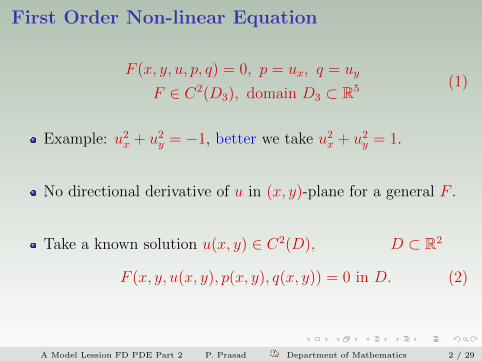
First Order Non-linear Equation

F (x, y, u, p, q) = 0, p = ux, q = uy

F ∈ C2(D3), domain D3 ⊂ R5(1)

Example: u2x + u2y = −1, better we take u2x + u2y = 1.

No directional derivative of u in (x, y)-plane for a general F .

Take a known solution u(x, y) ∈ C2(D), D ⊂ R2

F (x, y, u(x, y), p(x, y), q(x, y)) = 0 in D. (2)

A Model Lession FD PDE Part 2 P. Prasad Department of Mathematics 2 / 29

Charpit Equqtions

Taking x derivative of the PDE in (1)

Fx + Fuux + Fppx + Fqqx = 0

Using qx = (uy)x = (ux)y = py

Fppx + Fqpy = −Fx − pFu (3)

Beautiful, p is differentiated in the direction (Fp, Fq).Similarly

Fpqx + Fqqy = −Fy − qFu (4)


Charpit Equations contd..

For a given solution u(x, y) in (x, y)-plane, along one parameterfamily of curves given by

dx

dσ= Fp,

dy

dσ= Fq (5)

we havedp

dσ= −Fx − pFu (6)

dq

dσ= −Fy − qFu (7)

Further (note also for future reference)

du

dσ= ux

dx

dσ+ uy

dy

dσ= pFp + qFq (8)

Derived for a given solution u = u(x, y).



These, 5 equations for 5 quantities x, y, u, p, q are completeirrespective of the solution u(x, y).They are Charpit equations.

Given values (u0, p0, q0) at (x0, y0), such that(x0, y0, u0, p0, q0) ∈ D3

⇒ local unique solution of Charpit Equations with(x0, y0, u0, p0, q0) at σ = 0.

Autonomous system of five equations ⇒ 4 parameter family ofsolutions.(x, y, u, p, q) = (x, y, u, p, q)(σ, c1, c2, c3, c4).



Theorem Every solution of the Charpit’s equations satisfies (it isa part of Charpit E)

du

dσ= p(σ)

dx

dσ+ q(σ)

dy

dσ(9)



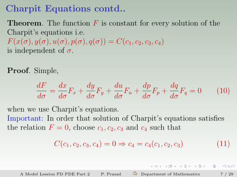
Theorem. The function F is constant for every solution of theCharpit’s equations i.e.F (x(σ), y(σ), u(σ), p(σ), q(σ)) = C(c1, c2, c3, c4)is independent of σ.

Proof. Simple,

dF

dσ=dx

dσFx +

dy

dσFy +

du

dσFu +

dp

dσFp +

dq

dσFq = 0 (10)

when we use Charpit’s equations.Important: In order that solution of Charpit’s equations satisfiesthe relation F = 0, choose c1, c2, c3 and c4 such that

C(c1, c2, c3, c4) = 0⇒ c4 = c4(c1, c2, c3) (11)


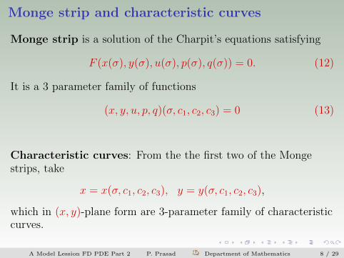
Monge strip and characteristic curves

Monge strip is a solution of the Charpit’s equations satisfying

F (x(σ), y(σ), u(σ), p(σ), q(σ)) = 0. (12)

It is a 3 parameter family of functions

(x, y, u, p, q)(σ, c1, c2, c3) = 0 (13)

Characteristic curves: From the the first two of the Mongestrips, take

x = x(σ, c1, c2, c3), y = y(σ, c1, c2, c3),

which in (x, y)-plane form are 3-parameter family of characteristiccurves.


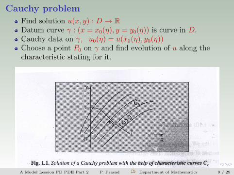
Cauchy problem

Find solution u(x, y) : D → RDatum curve γ : (x = x0(η), y = y0(η)) is curve in D.Cauchy data on γ, u0(η) = u(x0(η), y0(η))Choose a point P0 on γ and find evolution of u along thecharacteristic stating for it.


Solution of a Cauchy problem

For a general nonlinear equation,value of u is carried along acharacteristic not independently but together with values of p andq.

We need values of x0, y0, u0, p0 and q0 at P0 on datum curve asinitial data for Charpit’s equations at σ = 0.

A Model Lession FD PDE Part 2 P. Prasad Department of Mathematics10 /29

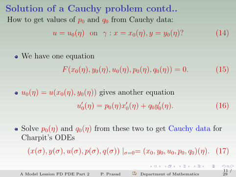
Solution of a Cauchy problem contd..How to get values of p0 and q0 from Cauchy data:

u = u0(η) on γ : x = x0(η), y = y0(η)? (14)

We have one equation

F (x0(η), y0(η), u0(η), p0(η), q0(η)) = 0. (15)

u0(η) = u(x0(η), y0(η)) gives another equation

u′0(η) = p0(η)x′0(η) + q0y′0(η). (16)

Solve p0(η) and q0(η) from these two to get Cauchy data forCharpit’s ODEs

(x(σ), y(σ), u(σ), p(σ), q(σ)) |σ=0= (x0, y0, u0, p0, q0)(η). (17)


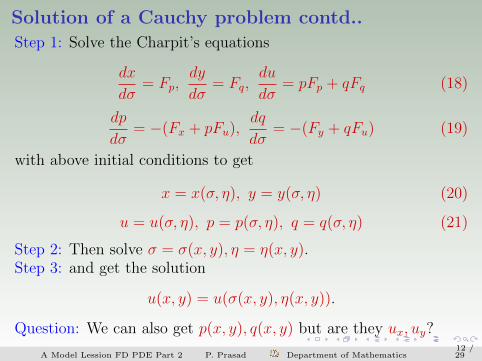
Solution of a Cauchy problem contd..Step 1: Solve the Charpit’s equations

dx

dσ= Fp,

dy

dσ= Fq,

du

dσ= pFp + qFq (18)

dp

dσ= −(Fx + pFu),

dq

dσ= −(Fy + qFu) (19)

with above initial conditions to get

x = x(σ, η), y = y(σ, η) (20)

u = u(σ, η), p = p(σ, η), q = q(σ, η) (21)

Step 2: Then solve σ = σ(x, y), η = η(x, y).Step 3: and get the solution

u(x, y) = u(σ(x, y), η(x, y)).

Question: We can also get p(x, y), q(x, y) but are they ux, uy?


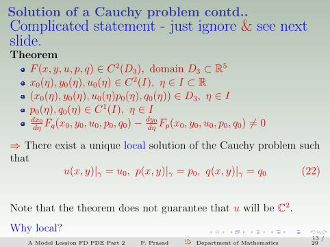
Solution of a Cauchy problem contd..Complicated statement - just ignore & see nextslide.Theorem

F (x, y, u, p, q) ∈ C2(D3), domain D3 ⊂ R5

x0(η), y0(η), u0(η) ∈ C2(I), η ∈ I ⊂ R(x0(η), y0(η), u0(η)p0(η), q0(η)) ∈ D3, η ∈ Ip0(η), q0(η) ∈ C1(I), η ∈ Idx0dηFq(x0, y0, u0, p0, q0)− dy0

dηFp(x0, y0, u0, p0, q0) 6= 0

⇒ There exist a unique local solution of the Cauchy problem suchthat

u(x, y)|γ = u0, p(x, y)|γ = p0, q(x, y)|γ = q0 (22)

Note that the theorem does not guarantee that u will be C2.

Why local?A Model Lession FD PDE Part 2 P. Prasad Department of Mathematics

13 /29

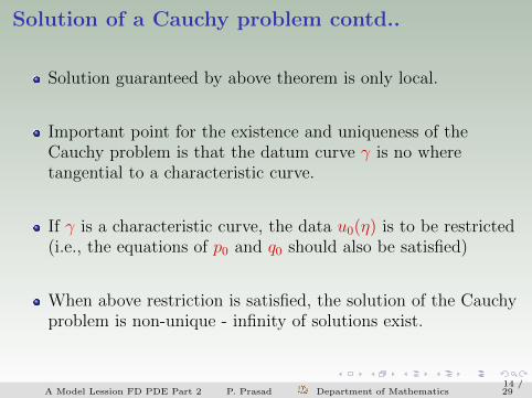
Solution of a Cauchy problem contd..

Solution guaranteed by above theorem is only local.

Important point for the existence and uniqueness of theCauchy problem is that the datum curve γ is no wheretangential to a characteristic curve.

If γ is a characteristic curve, the data u0(η) is to be restricted(i.e., the equations of p0 and q0 should also be satisfied)

When above restriction is satisfied, the solution of the Cauchyproblem is non-unique - infinity of solutions exist.


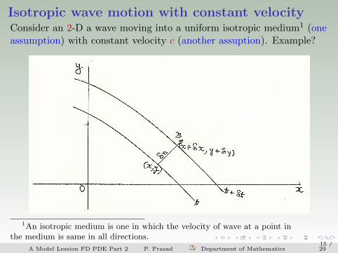
Isotropic wave motion with constant velocityConsider an 2-D a wave moving into a uniform isotropic medium1 (oneassumption) with constant velocity c (another assuption). Example?

1An isotropic medium is one in which the velocity of wave at a point inthe medium is same in all directions.


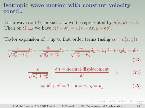
Isotropic wave motion with constant velocitycontd..

Let a wavefront Ωt in such a wave be represented by u(x, y) = ct.Then on Ωt+δt we have c(t+ δt) = u(x+ δx, y + δy).

Taylor expansion of u up to first order terms (using ct = u(x, y))

c√u2x + u2y

δt =ux√u2x + u2y

δx+uy√u2x + u2y

δy = n1δx+ n2δy = δn

(23)

c√u2x + u2y

=δn = normal displacement

δt= c (24)

⇒ p2 + q2 = 1; p = ux, q = uy. (25)


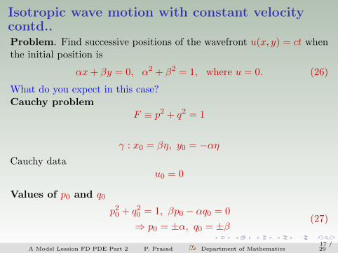
Isotropic wave motion with constant velocitycontd..Problem. Find successive positions of the wavefront u(x, y) = ct whenthe initial position is

αx+ βy = 0, α2 + β2 = 1, where u = 0. (26)

What do you expect in this case?Cauchy problem

F ≡ p2 + q2 = 1

γ : x0 = βη, y0 = −αηCauchy data

u0 = 0

Values of p0 and q0

p20 + q20 = 1, βp0 − αq0 = 0

⇒ p0 = ±α, q0 = ±β(27)


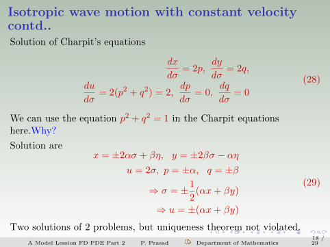
Isotropic wave motion with constant velocitycontd..Solution of Charpit’s equations

dx

dσ= 2p,

dy

dσ= 2q,

du

dσ= 2(p2 + q2) = 2,

dp

dσ= 0,

dq

dσ= 0

(28)

We can use the equation p2 + q2 = 1 in the Charpit equationshere.Why?

Solution arex = ±2ασ + βη, y = ±2βσ − αη

u = 2σ, p = ±α, q = ±β

⇒ σ = ±1

2(αx+ βy)

⇒ u = ±(αx+ βy)

(29)

Two solutions of 2 problems, but uniqueness theorem not violated.


Isotropic wave motion with constant velocitycontd..

Wavefrontsαx+ βy = ±ct. (30)

+ sign for forward propagating wavefront.

− sign for backward propagating wavefront.

Normal distance at time t from the initial position = ±ct.


We have presented the theory of characteristics of first orderPDEs briefly. It is based on the existence of characteristics curvesin the (x, y)-plane.

Along each of these characteristics we derive a number ofcompatibility conditions, which are transport equations and whichare sufficient to carry all necessary information from the datumcurve in the Cauchy problem into a domain in which solution isdetermined.

In this sense every first order PDE is a hyperbolic equation.


We have omitted a special class of solutions known as completeintegral, for which any standard text may be consulted.

Every solution of the PDE (1) can be obtained from a completeintegral.

We can also solve a Cauchy problem with its help.

Complete integral plays an important role in Physics.


So far we have discussed only a genuine solution (except for twoexamples in the case of quasilinear equations), which is validlocally.

We have seen that characteristic carry information about thesolution.

Characteristic curves are the only curve which can sustaindiscontinuities of certain types in the solution.

For a linear equation the discontinuities can be in the solutionand its derivatives, for a quasilinear equation thediscontinuities can be in the first and higher order derivatives.

for nonlinear equations the discontinuities can be in secondand higher order derivatives.


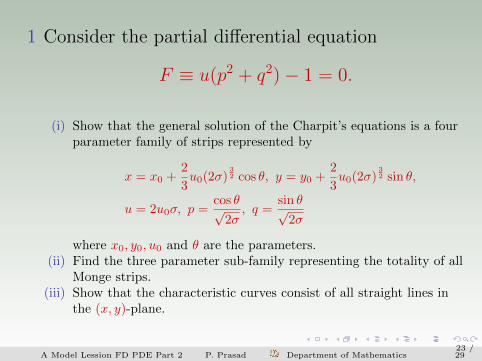
1 Consider the partial differential equation

F ≡ u(p2 + q2)− 1 = 0.

(i) Show that the general solution of the Charpit’s equations is a fourparameter family of strips represented by

x = x0 +2

3u0(2σ)

32 cos θ, y = y0 +

2

3u0(2σ)

32 sin θ,

u = 2u0σ, p =cos θ√

2σ, q =

sin θ√2σ

where x0, y0, u0 and θ are the parameters.(ii) Find the three parameter sub-family representing the totality of all

Monge strips.(iii) Show that the characteristic curves consist of all straight lines in

the (x, y)-plane.


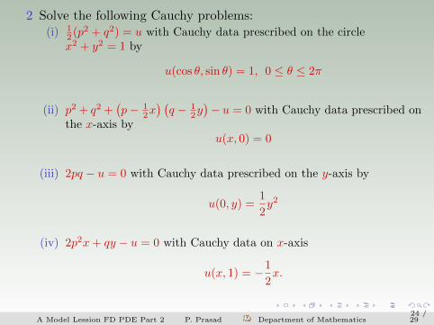
2 Solve the following Cauchy problems:(i) 1

2 (p2 + q2) = u with Cauchy data prescribed on the circlex2 + y2 = 1 by

u(cos θ, sin θ) = 1, 0 ≤ θ ≤ 2π

(ii) p2 + q2 +(p− 1

2x) (q − 1

2y)− u = 0 with Cauchy data prescribed on

the x-axis byu(x, 0) = 0

(iii) 2pq − u = 0 with Cauchy data prescribed on the y-axis by

u(0, y) =1

2y2

(iv) 2p2x+ qy − u = 0 with Cauchy data on x-axis

u(x, 1) = −1

2x.


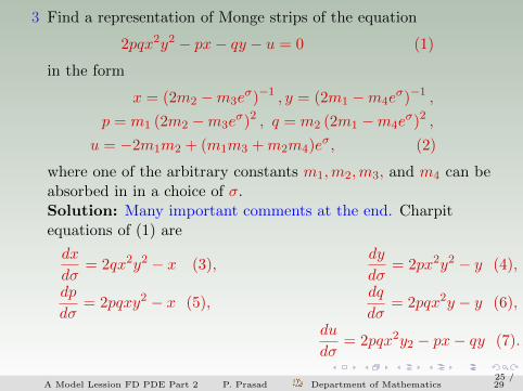
3 Find a representation of Monge strips of the equation

2pqx2y2 − px− qy − u = 0 (1)

in the form

x = (2m2 −m3eσ)−1 , y = (2m1 −m4e

σ)−1 ,

p = m1 (2m2 −m3eσ)2 , q = m2 (2m1 −m4e

σ)2 ,

u = −2m1m2 + (m1m3 +m2m4)eσ, (2)

where one of the arbitrary constants m1,m2,m3, and m4 can beabsorbed in in a choice of σ.Solution: Many important comments at the end. Charpitequations of (1) are

dx

dσ= 2qx2y2 − x (3),

dy

dσ= 2px2y2 − y (4),

dp

dσ= 2pqxy2 − x (5),

dq

dσ= 2pqx2y − y (6),

du

dσ= 2pqx2y2 − px− qy (7).


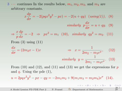
3 · · · continues In the results below, m1,m2,m3, and m4 arearbitrary constants.

xdp

dσ= −2(pqx2y2 − px) = −2(u+ qy) (using(1)), (8)

similarly pdx

dσ= u+ qy. (9)

⇒ x

p

dp

dx= −2 ⇒ px2 = m1 (10), similarly qy2 = m2. (11)

From (3) using (11)

dx

dσ= (2m2x− 1)x ⇒ x =

1

2m2 −m3eσ, (12)

similarly y =1

2m1 −m4eσ. (13)

From (10) and (12), and (11) and (13) we get the expressions for pand q. Using the pde (1),

u = 2pqx2y2 − px− qy = −2m1m2 + 9(m1m3 = m2m4)eσ (14).


3 · · · continues

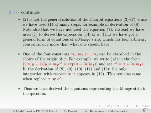
I (2) is not the general solution of the Charpit equations (3)-(7), sincewe have used (1) at many steps, for example in derivation of (8).Note also that we have not used the equation (7). Instead we haveused (1) to derive the expression (14) of u. Thus we have got ageneral form of equations of a Monge strip, which has four arbitraryconstants, one more than what one should have.

I One of the four constants m1,m2,m3,m4 can be absorbed in thechoice of the origin of σ. For example, we write (13) in the form(2m1y − 1)/y = m4e

σ = exp(σ + ln(m4)) and set σ′ = σ + ln(m4).In the derivation of (8), (9), (10), (11) and (12); the onlyintegration with respect to σ appears in (12). This remains samewhen replace σ by σ′.

I Thus we have derived the equations representing the Monge strip inthe question.


1 C. R. Chester. Techniques in Partial Differential Equations.McGraw-Hill, New York, 1971.

2 R. Courant and D. Hilbert. Methods of Mathematical Physics,vol 2: Partial Differential Equations. Interscience Publishers, NewYork, 1962.

3 L. C. Evans. Partial Differential Equations. Graduate Studies inMathematics, Vol 19, American Mathematical Society, 1999.

4 F. John. Partial Differential Equations. Springer-Verlag, NewYork, 1982.

5 P. Prasad. Nonlinear Hyperbolic Waves in Multi-dimensions.Monographs and Surveys in Pure and Applied Mathematics,Chapman and Hall/CRC, 121, 2001.

6 P. Prasad and R. Ravindran. Partial Differential Equations.Wiley Eastern Ltd, New Delhi, 1991.

7 J. D. Logan An introduction to nonlinear partial differentialequations, Wiley, 2008.


Thank You!


Documents

First Order Partial Differential Equation, Part - 2: Non