First Order System Response

7/23/2019 First Order System Response

http://slidepdf.com/reader/full/first-order-system-response 1/7

22..44..44:: FFiirrsstt OOrrddeerr CCiirrccuuiitt FFoorrcceedd RReessppoonnssee

Revision:June 12, 2010 215 E Main Suite D | Pullman, WA 99163(509) 334 6306 Voice and Fax

Doc: XXX-YYY page 1 of 7

Copyright Digilent, Inc. All rights reserved. Other product and company names mentioned may be trademarks of their respective owners.

Overview

In chapters 2.4.2 and 2.4.3, we were concerned with the natural response of electrical circuitscontaining a single energy storage elements. In this case, any sources in the circuit were isolatedfrom the circuit prior to determining the circuit response so that the circuit being analyzed containedno sources. Thus, the circuit response of interest was entirely due to the energy initially stored in thecircuit’s capacitors or inductors. In these cases, all voltages and currents in the circuit die out withtime.

In this chapter, we consider the case in which voltage or current sources are present in the first ordercircuit being analyzed. In this case, we must concern ourselves not only with the initial conditions inthe circuit, but also with any driving or forcing functions applied to the circuit. The response of asystem in the presence of an external input such as a voltage or current source is commonly calledthe forced response of the system. A primary difference between the natural response and the

forced response of a system is that, although the natural response of a system always decays to zero,the forced response has no such restriction. In fact, the forced response of the system will take thesame form as the forcing function, as time goes to infinity.

Before beginning this chapter, you shouldbe able to:

After completing this chapter, you should beable to:

• Write the differential equationsgoverning first order circuits (Chapters2.4.1, 2.4.2 and 2.4.3)

• Determine the time constant of a first

order electrical circuit from thegoverning differential equation(Chapters 2.4.1, 2.4.2, and 2.4.3)

• Determine the time constants of RL andRC circuits directly from the circuit(Chapters 2.4.2 and 2.4.3)

• Determine initial conditions on RL andRC circuits (Chapters 2.4.2 and 2.4.3)

• Write from memory the form of the stepresponse of a first order system(Chapter 2.4.1)

• Sketch the step response of a first order

system (Chapter 2.4.1)

• Write the form of the differential equationsgoverning forced first order electrical circuits

• Determine the time constant of a forcedelectrical circuit from the governing

differential equation• Write differential equations governing

passive and active first order circuits

This chapter requires:

• N/A



2.4.2: First Order Circuit Forced Response

www.digilentinc.com page 2 of 7


In this chapter, we will be concerned with the forced response of first order circuits. The differentialequations governing these circuits are still, as implied, first order – thus, the circuits presented herewill contain only a single energy storage element. Figure 1 shows two examples of forced first ordercircuits; Figure 1(a) is a forced RC circuit and Figure 1(b) is a forced RL circuit. The voltage sources

v s (t) in Figure 1 provide an arbitrary input voltage which can vary as a function of time. Without loss ofgenerality, we will concern ourselves only with determining the forced response of the voltages acrosscapacitors or the currents through inductors. In spite of the simplicity of the circuits shown in Figure 1,their analysis provides a framework within which to place the analysis of an arbitrary first orderelectrical circuit. These two circuits are, therefore, analyzed below in order to present the forcedsolution of an arbitrary first order differential equation.

(a) Forced RC circuit (b) Forced RL circuit

Figure 1. Forced first order circuit examples.

Tip:

In all circuits we analyze, we will define as unknown variables the voltages across capacitors and

the currents through inductors. We will then solve for these variables and determine any othernecessary circuit parameters from these variables.

In any electrical circuit, we can determine any circuit parameter from the voltages acrosscapacitors and the currents through inductors. The reason for this is that capacitor voltagesdescribe the capacitor energy storage and inductor currents describe the inductor energy storage.If we know the energy stored in all energy storage elements, we have completely characterizedthe circuit’s operating parameters – mathematically, we say that we have defined the state of thesystem. We will formalize this concept later when we discuss state variable models .

Examples of this concept, in the context of Figures 1 include:

• The voltage drop across the resistor in Figure 1(a) is: )t (v)t (v)t (v cs R −=

• The current through the capacitor in Figure 1(a) is: R

)t (v)t (v)t (i cs

R

−=

• The voltage drop across the resistor in Figure 1(b) is: )t ( Ri)t (v L R =






KCL at the positive terminal of the capacitor of the circuit shown in Figure 1(a) provides:

dt

)t (dvC

R

)t (v)t (v ccs=

− (1)

Dividing through by the capacitance, C, and grouping terms results in the governing differentialequation for the circuit of Figure 1(a):

)t (v RC

)t (v RC dt

)t (dvsc

c 11=+ (2)

KVL around the loop of the circuit of Figure 1(b) results in:

0=++−

dt

)t (di L)t ( Ri)t (v L

Ls (3)

Dividing through by the inductance, L, and rearranging results in the governing differential equation forthe circuit of Figure 1(b):

)t (v L

)t (i L

R

dt

)t (dis L

L 1=+ (4)

We notice now that the RC

1 term in equation (2) corresponds to

τ

1, where τ is the time constant of an

RC circuit. Likewise, we note that the

L

R term in equation (4) corresponds to

τ

1, where τ is the time

constant of an RL circuit. Thus, both equation (2) and equation (4) are of the form

)t (u)t ( ydt

)t (dy=+

τ

1 (5)

where τ is the time constant of the system, u(t) is the input to the system, and y(t) is the desiredsystem parameter (a voltage across a capacitor or a current through an inductor, for example).Equation (5) can be solved, given knowledge of the initial conditions on y(t), y(0) = y 0 . A blockdiagram of the system described by equation (5) is shown in Figure 2.

Figure 2. Block diagram of general forced first order system.






The solution to a forced differential equation can be considered to be formed of two parts: thehomogeneous solution or natural response (which characterizes the portion of the response due tothe system’s time constant and initial conditions) and the particular solution or forced response (whichcharacterizes the system’s response to the forcing function u(t) after the natural response has diedout). Thus, the system response y(t) can be expressed as:

)t ( y)t ( y)t ( y ph += (6)

where y h (t) is the homogeneous solution and y p (t) is the particular solution.

We will not attempt to analytically determine the solution of equation (5) for the general case of anarbitrary forcing function u(t); instead, we will focus on specific types of inputs. Inputs of primaryinterest to us will consist of:

• Constant (step) input functions

• Sinusoidal input functions

The study of circuit responses to these input functions is provided in later chapters.

We conclude this section with several examples in which we determine the differential equationsgoverning first order electrical circuits. Note that we make no attempt to solve these differentialequations – in fact, we cannot solve the differential equations, since we have not specified what theforcing functions are in the circuits below.






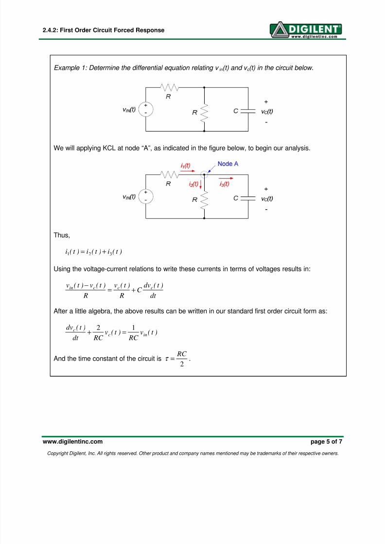
Example 1: Determine the differential equation relating v in (t) and v c (t) in the circuit below.

We will applying KCL at node “A”, as indicated in the figure below, to begin our analysis.

Thus,

)t (i)t (i)t (i321

+=

Using the voltage-current relations to write these currents in terms of voltages results in:

dt

)t (dvC

R

)t (v

R

)t (v)t (v cccin+=

−

After a little algebra, the above results can be written in our standard first order circuit form as:

)t (v RC

)t (v RC dt

)t (dvinc

c 12=+

And the time constant of the circuit is2

RC =τ .






Example 2: Determine the differential equation relating V in (t) and V out (t) in the circuit below.

+

-R

V IN (t)+

-

V OUT (t)

C

+

-

Consistent with our approach of defining variables as voltages across capacitors and currentsthrough inductors, we define the capacitor voltage as v c (t), as shown in the figure below. Also inthe figure below, node A is defined and the rules governing ideal op-amps are used to identify thenode voltage VA = 0V.

Applying KCL at node A in the circuit above gives:

)t (i)t (i21

=

The currents can be written in terms of the voltages in the circuit to provide:

dt

)t (dvC

R

)t (V cin=

− 0

The capacitor voltage can be written in terms of Vout (using KVL) as:

)t (v)t (V cOUT −=

Thus, the governing differential equation for this circuit can be written as:

∫−= dt )t (V RC

V inOUT

1

Note that this circuit is performing an integration.






Example 3: Determine the differential equation relating V in (t) and V out (t) in the circuit below.

As in example 2, we define node A is defined and use the rules governing ideal op-amps toidentify the node voltage V

A = 0V, as shown in the figure below.

+

-

V IN (t)+

-

V OUT (t)

+

-

R

C

Node A

(V A = 0V)

Writing KCL at node A directly in terms of the node voltages results in:

R

V

dt

)t (dV C OUT in

−=

So that:

dt

)t (dV RC V in

OUT −=

and the output voltage is proportional to the derivative of the input voltage.

Documents

First Order System Response