Embed Size (px)
Citation preview

Fiscal Governance after the Financial Crisis: A reviewA. Hughes Hallett
Working paper No. 2019/8 | August 2019 | ISSN 2516-5933
Data Analytics for Finance & Macro Research Centre
KING’S BUSINESS SCHOOL

1
Fiscal Governance after the Financial Crisis: A review1
Andrew Hughes Hallett
Kings College, University of London, and Copenhagen Business School
Abstract: Economists have traditionally used a
simple rule that restricts primary deficits to less
than a threshold given by the interest-growth rate
differential and existing debt in order to judge
fiscal sustainability. This rule derives from a single
period application of the government budget
constraint. It is not forward looking. In the
equivalent dynamic rule, the primary surplus
needs to match any expected, discounted increases
in public spending, the net interest on existing debt,
and preferences for extending debt relative to
changing taxes.
JEL classification: E62, H53, H63, I38;
Keywords: Sustainable public debt, primary deficit rules, fiscal space.
1 This paper was presented to the Economic Society of Australia, “Symposium on Lessons from the Global
Financial Crisis”, Griffith University, 7 March 2019. It reflects the lessons learned from joint research on
fiscal governance carried out with my colleagues: Floriana Cerniglia and Enzo Dia. However, I am
responsible for the interpretation placed on the results which emerged.
2
1. Introduction
All the advanced OECD economies were adversely affected by the Great Financial
Crisis, although some like Australia and Canada were less affected than those in Europe.
The common feature seems to have been a marked worsening of their public debt burdens,
and an inability to prevent their budget balances from deteriorating during the crisis and
(more importantly) an inability to successfully repair their fiscal balances after the crisis.
This paper reviews the rules we currently use, and those currently recommended,
for limiting the size of fiscal deficits and preventing the kind of permanent debt increases
we have seen over the past years. The principal focus is on which of these rules work, and
on explaining why they very often do not work.
The simplest rules (using IMF recommendations) are based on restrictions on
public spending, raising sufficient revenues, and/or maintaining strict balanced budget
restrictions. But as such, they do not place or guarantee any explicit restraints on the
underlying stock of public debt; and they suffer from a general "endogeneity problem"
(that is: by placing restrictions on revenues, public spending or the budget balance will
automatically change income levels and hence cause us to miss the outcomes previously
planned for those target variables).
The next type of rule (currently favoured by the IMF staff) is one designed to keep
public debt levels constant - or move them up or down by specified amounts, within the
current period – and then to be repeated in following periods as needed (Blanchard, 2019).
This rule notes that the change in the debt burden (i.e. the budget surplus) will be the
difference between the interest payable on the existing debt burden and the current rate of
output growth, multiplied by the current debt burden. Calculating this quantity gives a
minimum value for the primary target surplus if we don't want debt to increase. A smaller
surplus will allow debt to increase; a larger surplus will force debt to decrease. The
difficulties with this rule are:

3
1. It implicitly assumes that the responses of taxes or public spending to the policy
changes necessary to get the primary surplus we need, are infinitely and instantan-
eously elastic. This is most unlikely to be the case in practice.
2. You need to make error free, unbiased forecasts of the future interest rate payable
on the average stock of debt (relatively easy to calculate) and of future output
growth (not so easy to calculate).
3. The growth adjusted interest rate must allow for the possibility of default risk
premia and inflation risk premia; and for the fact that the CPI inflation rate to be
subtracted from the interest rate will be different from the GDP inflation rate to be
subtracted from the growth rate (we need to work in real terms).
4. Sensitivity to forecast or any other errors can easily destabilise the stock of debt,
adding to the burden in bad times in a way that cannot be retrieved at a later time.
Numerical simulations of the evolution of debt under this control rule in the US and UK
show: i) it has consistently failed to prevent debt growing at different times over the past
50 years; ii) it has failed to bring down debt even when actual primary surpluses have
exceeded the threshold values specified by the rule. Hence, this rule is neither sufficient
nor necessary to control debt or to ensure public finances remain sustainable.
2. The performance of traditional debt stabilisation rules
2.1 Theory
The standard text-book rule for stabilising public debt requires the government
to obtain a primary surplus St greater than or equal to the difference between the
interest rate currently payable on outstanding debt, rt, and the current rate of
growth of nominal GDP ρt, multiplied by the existing debt to GDP ratio Bt:
St ≥ (rt − ρt)Bt. (1)
How can a government implement such a rule? When planning the budget for
the following year, the government needs to forecast the value of the difference rt −
ρt. If the government plans to reach a certain target for the debt to GDP ratio, Bt, in
the future, it needs to plan a sequence of expected surpluses over those years to

4
arrive at the desired target. In the following period the government needs to verify
the results achieved so far, to renew the forecast of the relevant variables in the
light of new information, and to define a new set of surpluses. The rule therefore
requires a process based on forecasting forward looking data, plus a feedback
adjustment for when new information on past failures and on future expected
interest rates/growth rate values becomes available:
Et−1[St] ≥ Et−1[rt − ρt]Bt. (2)
The forecasting error when predicting a sequence of future expected values for the
difference rt − ρt will be almost entirely due to GDP shocks since rt is to a large
extent (but not completely) predetermined.2 Since no country is financed entirely
with short-term debt, only a fraction of the outstanding debt in each period will
be refinanced at current interest rates. For example, if the average life of outstanding
debt is 10 years,3 on average only one tenth of the outstanding stock of debt needs to
be rolled over at the current interest rate and refinanced each year. Correspondingly
any change in interest rates will affect only one tenth of the debt stock.
More generally, if debt maturity spans n years, the expected interest rate
applicable to the next budget is rt =(𝑛−1
𝑛) ��𝑡+
1
𝑛E(r𝑛𝑡+1), where r t is the historical
cost of outstanding debt (a weighted average of past interest rates) and E[rnt+1] is the
expected cost of newly issued debt.
By contrast, since the rate of growth of nominal GDP is the sum of the rate of
growth of real GDP and of inflation. Both are typically I(1) series: the government
needs to be able to forecast the interaction between two random walk series with drift,
ρt = Et(gt+1) + Et(πt+1) + Et(gt+1∗ πt+1), where gt is the rate of growth of real GDP
at time t and πt is the inflation rate at time t. Typically, we ignore the last term as
second order small although this may not always be true in discrete time applications.
That said, the larger forecasting errors normally occur during recessions since the
2 rt represents the effective rate of interest payable on the stock of current and past debt. 3 For example, the average term to maturity of debt in Italy is 6.7 years, whereas that in the United Kingdom is 14 years

5
volatility of the series is typically clustered during downturns. These errors can be
substantial. During the last recession the output gap was, in most countries, 5 − 7 per-
cent and the deflation rate was around 2 percent. As a result, the typical value for ρt
was around 10 percent below trend. To pretend that the growth rate will remain
roughly constant in the next period(s) would be a mistake. Interest rates may also not
remain constant in recessions. Nevertheless, the interest rate to be applied to newly
issued debt, on the average cost of debt, is rather small in most countries compared to
errors/variations in the growth rate.
Yet, even if these approximation errors are small, there are further problems
with (1). When a recession occurs, any debt reduction plan may be suspected of
being not feasible or not credible. Second, the stabilisation rule, (1), will require a
massive dose of austerity which makes the recession deeper. The government is
then forced to choose between debt stabilisation that risks spiraling into an even
worse recession, or fiscal policy requiring more debt to reduce the output gap. Any
government may be expected to choose the latter path for economic and political
reasons, so long as financial markets or international institutions are willing to
provide credit. Either case will attract additional risk premia - making existing and
future debt less sustainable than previously predicted.
Alternatively, a government whose fiscal space is sufficiently large may choose to
adopt an expansive fiscal policy while keeping to a long term debt target, by
extending the stabilisation plan over a longer horizon. However, since any debt
could be accommodated that way, it may become difficult to commit to any specific
path and the available fiscal space may become tight for countries already holding
large amounts of debt. In practice, if the government cannot inflate its debt away to
achieve its target because debt is denominated in foreign currency, or because the
country has no control over monetary policy, the maturity extension exercise has to
become coercive through some form of default.
With these comments in mind, it is worthwhile to review what the traditional
stabilisation rule calculates. At each t, the existing stock of debt, Bt, is known. But

6
the growth adjusted interest rate is more complicated. In nominal terms, to match
how debt is recorded in national accounts, (1) contains:
𝐸𝑡(𝑟𝑡) − 𝐸𝑡(𝜌𝑡) = ∑ 𝑤𝑡−𝑗𝑇𝑗=1 𝑟𝑡−𝑗 + 𝑤𝑡𝐸𝑡(𝑟𝑡) − 𝐸𝑡(𝜌𝑡+1) (3)
where T represents the oldest maturity held, and wt is the proportion of maturity t in
total debt. Hence evaluated in real terms to reflect how the final outcomes for
consumption, investment, and the debt to GDP ratio will react to different levels of
debt, the corresponding term is:
Et(r t)−Et(gt) = ∑ 𝑤𝑡−𝑗𝑇𝑗=1 (𝑟𝑡−𝑗 − 𝜋𝑡−𝑗) + 𝑤𝑡𝐸𝑡(𝑟𝑡 − 𝜋𝑡) − 𝐸𝑡(𝜌𝑡+1) + 𝐸𝑡(𝜋𝑡+1) (4)
≠ ∑ 𝑤𝑡−𝑗𝑇𝑗=1 𝑟𝑡−𝑗 − 𝐸𝑡(𝜋𝑡) − 𝐸𝑡[𝜌𝑡+1 − 𝐸𝑡(𝜋𝑡+1)], (5)
where rt is the real interest rate on debt at t. The lower expression is the growth
adjusted interest rate that would be used if the standard debt stabilisation rule is
defined in real terms. In the standard framework, inter-temporal optimisation is not
necessary because the institutional framework of the models is extremely simple.
But when considering a more realistic environment, inter-temporal optimisation
will become necessary for a number of reasons:
i) To balance the benefits of raising taxes now against extending debt (and hence
raising taxes later).
ii) Because the expected inflation terms do not cancel out between rt and ρt
as usually assumed when the standard rule is applied.
iii) Because rt, πt and ρt are jointly dependent, and also jointly dependent over
time.
iv) Because adjustment costs in tax revenues and spending are not zero. So we
should expect incomplete adjustments over specific time intervals.
v) Since fiscal policy is not in real time, any budget surplus must be planned in
advance on the basis of the available information regarding future variables,
including the expected trend in entitlement spending.
Do points i) to v) matter? Fig. 1 illustrates the path that current debt would take if
the traditional primary surplus rule was applied consistently in the OECD. To see
7
the implications, we proceed as follows. The law of motion of the debt ratio is
Bt+1 = Bt + (rt − ρt)Bt − St. (6)
Next, we define a similar path for “controlled” debt; that is the path you would get if
the traditional primary surplus rule had been applied each year by generating
primary surpluses equal to (2). Defining Bt as controlled debt at time t under the
standard assumptions that nominal output and interest costs are random walks with
drift, we get:
𝐸𝑡(𝑟𝑡+1) = 𝑟𝑡; 𝐸𝑡(𝜌𝑡+1) = 𝜌𝑡 ; and ��𝑡+1 = ��𝑡+(𝑟𝑡 − 𝜌𝑡)��𝑡 + (𝑟𝑡−1 − 𝜌𝑡−1)��𝑡 (7)
Since rt − rt−1≠ 0 and ρt − ρt−1 ≠ 0, it now follows that Bt+1 =/ Bt. Hence the
standard primary surplus rule does not necessarily produce constant debt; or
indeed falling debt if that had been planned. In this world, it is not a reliable way
to achieve debt control.
2.2 Evidence
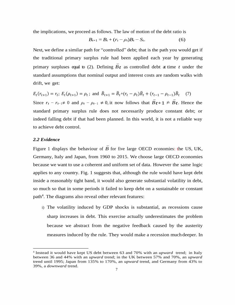
Figure 1 displays the behaviour of B for five large OECD economies: the US, UK,
Germany, Italy and Japan, from 1960 to 2015. We choose large OECD economies
because we want to use a coherent and uniform set of data. However the same logic
applies to any country. Fig. 1 suggests that, although the rule would have kept debt
inside a reasonably tight band, it would also generate substantial volatility in debt,
so much so that in some periods it failed to keep debt on a sustainable or constant
path4. The diagrams also reveal other relevant features:
i) The volatility induced by GDP shocks is substantial, as recessions cause
sharp increases in debt. This exercise actually underestimates the problem
because we abstract from the negative feedback caused by the austerity
measures induced by the rule. They would make a recession much deeper. In
4 Instead it would have kept US debt between 63 and 70% with an upward trend; in Italy
between 36 and 44% with an upward trend; in the UK between 57% and 70%, an upward
trend until 1995; Japan from 135% to 170%, an upward trend, and Germany from 43% to
39%, a downward trend.

8
addition, the degree of austerity necessary to stabilise debt by abiding by the
rule is likely to be large, since the rule would impose very quick fiscal
corrections. These policies would not be viewed as feasible or credible.
ii) Many of the downward corrections that we observe are due to unexpected in-
flation, particularly during the late 1970s. When monetary policy becomes
independent, the rule will require larger surpluses.
We can now analyse the actual behaviour of governments by comparing the paths
obtained for controlled debt Bt with those of actual debt Bt; and by comparing the
primary surpluses necessary to control debt with the corresponding actual primary
surpluses. Debt levels have increased steadily in most countries in recent years,
and these rises in debt have almost always been ascribed to a lack of fiscal
discipline of the kind required by the traditional rule. We can test that proposition
directly by comparing if actual primary surpluses St shown above were above or
below the necessary threshold (rt − ρt)Bt. This is done in Figures 2 and 3 for the
United States and United Kingdom respectively.
9
Figure 1: Controlled debt paths for selected OECD countries
60 65 70 75 80 85 90 95 00 05
60
10 60
63
64
65
66
67
68
69
70
71
56
58
60
62
64
66
68
70
72
60 65 70 75 80 85 90 95 00 05
60
10
60 65 70 75 80 85 90 95 00 05
60
10
32
34
36
38
34
42
44
38
40
41
42
43
60 65 70 75 80 85 90 95 00 05
60
10
13.0
13.5
14.0
14.5
15.0
15.5
16.0
16.5
17.0
60 65 70 75 80 85 90 95 00 05
60
10
United States United Kingdom
Italy Germany
Japan
39

10
Figure 2: Controlled debt/deficits: United States of America
Figure 3: United Kingdom
First, it is of interest that the actual debt levels in the US have been below the
controlled debt path for most of the period before 2007, with the exception of the
early 1990s and after 2005. But the primary surpluses were below (not above) the
required threshold, which explains why debt was on a rising path from 1980
onwards (1995-2000 excepted when primary surpluses were large enough to prevent
that). This result is consistent with the evidence of Ardagna et al (2007) and Bohn
(2011) suggesting that the US Federal government has adjusted revenues and
expenditure to stabilise debt over its history up to 1998.5 However, controlled debt
5 Jones and Joulfaian (1992) and Bohn (2011) analysed the stability of public debt in the United States by testing the response of the primary surplus to the level of the stock of debt. They find a statistically significant and economically relevant response, using data covering the whole history of the country. Mendoza and Ostry (2008) meanwhile used the
40
50
60
70
80
90
100
110
120
-12
-8
-4
0
4
8
60 65 70 75 80 85 90 95 00 056
0
10
Controlled debt path
Actual Debt path
Threshold value Primary surplus
60 65 70 75 80 85 90 95 00 056
0
10
30
40
50
60
70
80
90
100
60 65 70 75 80 85 90 95 00 05
60
10 60 65 70 75 80 85 90 95 00 056
0
10
-12
-8
-4
0
4
8
Controlled debt path
Actual Debt path
Threshold value Primary surplus

11
does not fall even when primary surpluses are large enough - implying that the
traditional rule was not the correct rule to reduce debt, and that the US government
had achieved better results by other means (fig. 2).
Compare the primary surpluses to the threshold necessary to make debt go
down: St > (rt − ρt)Bt. We find the primary surplus (red) was in deficit and mostly
below the threshold (blue) till 1977; equal to it or above to 1980; below it again in
1980 to 1995; then above it for 1996-2001; and clearly below it in 2001-2015. So
the US did not keep to the traditional rule very often before 1994, yet debt remained
below 1960s levels until 1990. In the Clinton era the Federal government achieved
primary surpluses above the threshold from 1996 until 2001, but then spectacularly
failed to do so from 2001-2015. However debt remained close to the initial level till
2007. The evidence for the United States therefore suggests that the traditional rule
has been virtually irrelevant until 2001.
Now look at the UK, fig 3. Once again controlled debt never falls, which again
implies that the traditional rule was not the correct rule to use to reduce debt. In
contrast, actual debt fell to 1990 and from 1997-2002 which implies that the UK found
an alternative rule (the fiscal deflation and pro-growth policies of the late Thatcher and
early Blair regimes). In this case also it shifted upwards in the years from 2008 on-
ward, following the crisis, and it has not reverted back. The UK authorities did satisfy
the traditional rule threshold until 1981, from 1986 to 1990 and from 1997 to 2001.
But they violated it from 1990 to 1996 and from 2001 to 2014. Nevertheless, despite
these outcomes, the United Kingdom has achieved debt levels below the controlled
debt path for more than forty years.
There are a variety of reasons why the traditional rule might have failed. First,
the primary surplus may not be able to adjust indefinitely without political or dis-
model to analyse the behaviour of German and US states, finding that if fiscal transfers are not included in the primary surplus, the US and German state governments pursued unsustainable fiscal policies.

12
tortionary costs, or because it demands changes that are beyond the economy’s
fiscal capacity. Second, it takes time for spending and tax changes to be debated
and take effect. If there is any delay in interest rates rising, or if inflation
expectations run ahead of actual inflation, the rule will generate a lower primary
surplus threshold than is warranted—leading policymakers to assume they have
more fiscal space than they actually have. Policymakers will then take on more
debt than they should and the ability to stabilise debt is lost. Third, it is a mistake
to assume that tax and spending changes are infinitely elastic, if for no other reason
there is persistence in entitlement spending and tax changes take time to take effect.
All three failures are consequences of having derived the traditional rule from
repeated applications of the government’s current budget constraint instead from a
consistent application of their inter-temporal budget constraint.
3. An inter-temporal framework for choosing debt and taxation
So what is the best way out of this difficulty; that is, to produce a rule that accounts for the
forward looking variables, predictable debt dynamics and the possibility of inter-temporal
trade-offs?
What the traditional rules above all leave out is the impact of rising entitlement spending
on debt, and how to control that spending. To illustrate how to proceed, this section
develops the equivalent debt control rule for that case. Given entitlement spending,
predictable over a few periods, this obviously allows for a trade-off between "tax now"
policies versus "tax later" policies (i.e. whether to use new debt to finance current
spending; or to use tax financing to cover that spending). But the dynamics of debt
accumulation must also be taken into account. So the analysis necessarily becomes more
complicated and technical. But the final result is only slightly more complicated than the
rule we had before, yet is one easily calculated by computer.
To start, we derive an inter-temporal decision framework for a government that

13
internalises any expected costs arising from raising revenues and issuing taxes,
under the assumption that a significant share of expenditure consists of entitlement
spending that may be treated as an exogenous stochastic process for the foreseeable
future. Our approach is based on an explicit recognition that policy discussions of
government spending are generally carried out on the basis that there is a clear-cut
difference between discretionary spending, and entitlement spending where funding
is mandatory unless specific reforms are proposed in Parliament. Entitlement
spending therefore includes all those categories of expenditure that do not have to
be approved annually since existing laws give agents rights to certain benefits or
services until reforms are called for. Two examples are social security (or social
benefits), and the compensation of employees. By contrast, discretionary spending
is composed of those expenditures that politicians have to vote on an annual or ad
hoc basis in order for them to take place. Discretionary spending also includes
categories of intermediate consumption that need to be voted annually in budgetary
sessions even if they then recur for several years.6 Accordingly, we assume that
public expenditure Gt is composed of entitlement spending Et and discretionary
spending Vt, where entitlement spending is an exogenous stochastic process
Gt = Et + Vt. (8)
The primary deficit Dt is the difference between expenditure Gt and tax revenues Tt –
where total expenditures are total general government expenditures net of interest
payments, while taxes include all general government revenues:
Dt = Gt − Tt = −St. (9)7
By substituting the deficit from Equation (9) into the law of motion of debt, Eq. (6),
we get taxes equal to (in each period):
6 The share of discretionary spending is typically about 1/3 of total government spending in
the OECD. A figure this size is relatively large when compared to the estimated residuals
of the auto-regressive processes usually used to measure the share of expenditures not
predetermined. However, it is smaller than assumed in econometric models that treat
government spending as fully exogenous [Coricelli and Fiorito, 2013]. 7 All variables are defined as ratios to GDP.

14
Tt = Gt − Bt + (1 + 𝑟𝑡−1 − 𝜌𝑡−1)𝐵𝑡−1. (10)
To keep the model tractable we assume that discretionary spending is financed with
tax revenues (but borrowing is allowed to cover entitlement spending):
Vt = τ Tt (11)
and thus Tt = 𝜓[Et – Bt + (1+rt-1 - ρt-1) Bt-1] (12)
where 1/(1-𝜏) = 𝜓 and 0 < τ < 1. Since discretionary spending is smaller than
entitlement spending, this assumption does not impose any restrictions. The choice
of funding by taxation or debt is now made for a given or predicted composition of
discretionary and entitlement spending.
Although Eq. 12 is standard, this formulation highlights that, as long as the costs
imposed by raising taxes are not linear, any convex cost on Tt generates an adjustment
cost on the stock of debt.8 Together, these costs impose a ceiling on debt. Eq. 12 can
now be rewritten as
𝑇𝑡 = 𝜓[𝐸𝑡 − Δ𝐵𝑡 + (𝑟𝑡−1 − 𝜌𝑡−1)𝐵𝑡−1] (13)
As a consequence, whenever linear or non-linear cost functions for taxes apply, the
problem becomes dynamic even without assuming non-linear cost functions for the
stock of debt or its adjustment.
Our modeling strategy is therefore different from the standard versions which
analyse the stock public debt as a sequence of period by period independent budget
constraints, without recognising the inter-temporal constraints. In our approach, the
objective function of policymakers is to provide the chosen expenditures while
minimising taxes and interest costs:9
𝐺𝑂𝐹 = 𝐸𝑡 + 𝜁𝑉𝑡 +𝛿
2𝑉𝑡
2 − 𝜈𝑇𝑡 −𝜙
2𝑇𝑡
2 −𝜄
2𝐵𝑡
2 − 𝑟𝑡𝐵𝑡 (14)
Hence entitlement spending generates linear benefits that we normalise to one,
8 The convexity assumption is supported by the empirical results of Agell (1996) and Agell et al (1996) suggesting that the distortionary effects of taxation are small for low levels of taxation, but they grow rapidly as taxes increase. 9 The constraint we impose is dynamic because it includes both flows and stocks.

15
and discretionary spending generates both linear and convex benefits whose size is
defined by the ζ and δ parameters. Similarly, ν and ϕ define linear and non-linear
cost parameters associated with tax revenues. They include both resource costs
induced by distortionary taxation, and political economy restrictions on government
behaviour induced by the voters’ aversion to taxes. Finally, the servicing of debt
imposes a standard interest cost rt. But the government needs also to internalise
any non-linear cost, β, caused by non-linearly increasing risk premia on the interest
cost, or by the voters’ aversion to public debt. Importantly, since we assume a finite
value of β, we do not consider the case where debt issuance becomes impossible.
Policymakers now maximise (14), subject to (12) and equations that define the
stochastic process of expenditure, interest rates, and GDP growth. For example, we
might model the latter as exogenous AR(1) processes:
𝐸𝑡+1 = 𝐸𝑡 + 𝛼 + 𝜂𝑡+1 (15)
𝑟𝑡+1 = 𝑟𝑡 + 𝛽 + 𝜀𝑡+1 (16)
𝜌𝑡+1 = 𝜌𝑡 + 𝛾 + 𝜃𝑡+1 (17)
where ηt+1, Et+1, and θt+1, represent i.i.d. random shocks with zero mean and constant
variances. Defining d as the discount factor, this leads to the Lagrangian form of the
problem:
Λ𝑡 = 𝑑𝑡{𝐸𝑡 − 𝛾𝑇𝑡 −𝛼
2𝑇𝑡
2 −𝜄
2𝐵𝑡
2 − 𝑟𝑡𝐵𝑡
+𝜇𝑡[𝑇𝑡 − 𝜓(𝐸𝑡 − 𝐵)𝑡 − 𝜓(1 + 𝑟𝑡−1 − 𝜌𝑡−1)𝐵𝑡−1]} (18)
where γ = ν − ζτ and 𝛼 = ϕ − δτ 2. The term in α represents the non-linear cost of
taxes, net of benefits, obtained from discretionary spending. Similarly, γ measures
the linear cost of taxes net of benefits from discretionary spending. Tax revenues are
a control variable, while debt is a state variable. The first order conditions for this
problem are as follows:
𝜕Λ
𝜕𝑇𝑡= − 𝛾 − 𝛼 + 𝜇𝑡 = 0 (19)
𝜕Λ
𝜕𝑩𝑡= − 𝜄𝐵𝑡 − 𝑟𝑡 + 𝜓𝜇𝑡 − 𝑑𝜓(1 + 𝑟𝑡 − 𝜌𝑡)𝜇𝑡+1 (20)
16
𝜇𝑡 = 𝛾 + 𝛼𝑇𝑡 (21)
Now, following Cerniglia et al (2018), define β = ι (1 − τ ) and υ = 1 – τ 10 to get
𝑑(1 + 𝑟𝑡 − 𝜌𝑡)𝜇𝑡+1 = 𝜇𝑡 −𝜄
𝜓𝐵𝑡 −
1
𝜓𝑟𝑡 = 𝜇𝑡 − 𝛽𝐵𝑡 − 𝜈𝑟𝑡 (22)
Next, eliminating µt between Eq. 21 and Eq. 22, we obtain:
𝑑(1 + 𝑟𝑡 − 𝜌𝑡)𝑇𝑡+1 =1
𝑑𝑇𝑡 −
1
𝑑𝛼[−𝛾(1 − 𝑑) + (𝜈 + 𝑑𝛾)𝑟𝑡 − 𝑑𝛾𝜌𝑡 + 𝛽𝐵𝑡 (23)
Finally, we can now substitute for the value of Tt in Eq. 9 to obtain:
(1 + 𝑟𝑡 − 𝜌𝑡)(𝐺𝑡+1 − 𝐷𝑡+1) =1
𝑑(𝐺𝑡 − 𝐷𝑡) −
1
𝑑𝛼[−𝛾(1 − 𝑑) + (𝜈 + 𝑑𝛾)𝑟𝑡 − 𝑑𝛾𝜌𝑡 + 𝛽𝐵𝑡]
(24)
and
Δ𝐵𝑡+1 = (1 + 𝑟𝑡 − 𝜌𝑡)𝐺𝑡+1 −1
𝑑𝐺𝑡 − (𝑟𝑡 − 𝜌𝑡)𝐵𝑡+1 + [(𝑟𝑡 − 𝜌𝑡)2 + 2(𝑟𝑡 − 𝜌𝑡)]𝐵𝑡 +
1
𝑑𝐵𝑡 −
1
𝑑(1 + 𝑟𝑡−1 − 𝜌𝑡−1)𝐵𝑡 +
1
𝑑𝛼[−𝛾(1 − 𝑑) + (𝜈 + 𝑑𝛾)𝑟𝑡 − 𝑑𝛾𝜌𝑡 + 𝛽𝐵𝑡] (25).
At this point, we have derived a law of motion for government debt showing how
expenditure shocks are entirely absorbed by new debt issuance. Note: the responses
of new issuances to the existing stock of bonds and to market interest rates are both
functions of the relative weights of the non-linear cost of debt and taxes. For higher
levels of the tax parameter α, the impact of interest rates and the past stock of debt
declines. The impact of interest rates rises with the linear cost term γ, while the
impact of the past stock of debt is large for larger values of β reflecting the convex
costs of the stock of debt.
This second order difference equation in 𝐵𝑡+1 (which includes the debt implicit
in the anticipated deficits 𝐷𝑡+1 and current deficit 𝐷𝑡) cannot be solved with the
standard techniques proposed by Sargent (1979) because rt is part of the intercept
term and also of the slope. The roots in the solutions are thus time varying.
10 Thus 𝜄 < 𝛽 and 𝜈 < 1. In practice the parameters of this model are likely to vary over time and different
economies.
t

17
5. The new solvency rule
Finally, the law of motion derived in Equation (25) can be rewritten to make the
role of primary deficits and surpluses explicit:
Δ𝐵𝑡+1 = (1 + 𝑟𝑡 − 𝜌𝑡)𝐺𝑡+1 +1
𝑑𝐺𝑡 + (𝑟𝑡 − 𝜌𝑡)(1 + 𝑟𝑡−1 − 𝜌𝑡−1)𝐵𝑡−1 −
(𝑟𝑡 − 𝜌𝑡−1)Δ𝐷𝑡 +1
𝛼𝐷𝑡 +
1
𝑑𝛼[−𝛾(1 − 𝑑) + (𝜈 + 𝑑𝛾)𝑟𝑡 − 𝑑𝛾𝜌𝑡 + 𝛽𝐵𝑡] (26)
which yields a rule that defines a primary surplus sufficient to stabilise debt:
−𝐷𝑡 = [𝑑(1 + 𝑟𝑡 − 𝜌𝑡)𝐺𝑡+1 − 𝐺𝑡] + 𝑑(𝑟𝑡 − 𝜌𝑡)(𝐵𝑡 − 𝐷𝑡+1) −
1
𝛼[−𝛾(1 − 𝑑) + (𝜈 + 𝑑𝛾)𝑟𝑡 − 𝑑𝛾𝜌𝑡 + 𝛽𝐵𝑡] (27)
where υ = 1 − τ . This rule defines a threshold above which the primary surplus will
reduce the debt ratio, and below which debt increases. It is however, quite different
from the standard textbook rule which would be −Dt = (rt − ρt)Bt in this notation.
In fact (27) contains three terms. a) The first represents the discounted
growth adjusted increase in total public spending relative to national income. b)
The second is the counterpart to the standard textbook rule, but discounted and
adjusted for the expected/planned surplus next period. c) The last term represents
all the preference factors (and post-tax interest rate) that arise because we need to
account for inter-temporal optimising behaviour: that is, for the choice between
raising taxes now; or to extend debt to tax later to finance current or future
spending liabilities. The trade-off between using taxes vs. debt is likely to dominate
(27) since the remaining terms will be small compared to (β/α)Bt.
The practical implication of (27) is that the old period-by-period criterion is no
longer sufficient to ensure sustainable public finances once entitlement spending
enters the story. Instead, we need to impose a condition that public spending shall not
grow faster than national income by a certain margin and then subtract off the effect
of preferring to tax now vs. increasing debt and tax later using expected growth to
compensate. But none of these choices can be made without cost or restriction.
When policymakers have a strong aversion to debt, so that β is larger, or when

18
interest costs are high, the primary surplus required is larger. By contrast, the
higher the distortions caused by high tax revenues relative to income, the lower is
the primary surplus required since debt becomes a more attractive tool to smooth
out any expenditure shocks.
5. Conclusions
This paper has introduced a primary surplus rule to ensure stable and sustain-
able public finances in a dynamic world with entitlement spending liabilities. To do
that requires us to move from a static rule based on the government’s current
budget constraint, to an inter-temporal rule, since policymakers have to trade off
using taxes now to fund current (future) spending vs. using debt, and future taxes, to
fund that spending. Our rule therefore replaces the traditional period-by-period rule,
and responds to three different sets of variables: a) the growth of public spending
relative to the growth in national income; b) the familiar growth adjusted interest
payments due on current debt, now discounted and adjusted for anticipated future
primary surpluses; and c) the effects of choosing between taxing now, or later by
increasing current debt.
Thus, in a dynamic world, the primary surplus needs to at least match any expected
discounted increases in public spending, the net interest on existing debt, and terms
reflecting the preference (or cost) for extending debt relative to the cost of changing
taxes. When policymakers have a strong aversion to debt (β is large), or if interest costs
relative to growth are high, the primary surplus required is larger. But if the distortions
due to high taxes relative to income are large, a lower primary surplus is required since
debt becomes a more attractive tool to smooth spending shocks.
It is important to note that some countries have capped spending growth to be no
more than national income growth, alongside a standard primary surplus rule or a
balanced budget rule. A prominent example is the Euro-zone’s fiscal compact. But
none have accounted for the impact of preferences when spending is dynamic; or for
the projected impact of interest payments on future deficits; or have considered

19
limiting spending growth to the available space, instead of a hard limit to GDP
growth which would institutionalise austerity policies in every recession. Thus, none
of those operating rules are sufficient to guarantee fiscal sustainability. But they
might be simple and possibly effective approximations to our more complicated
rule. It remains to be determined if (and when) that is true.
References
Agell, J., November 1996. Why Sweden’s welfare state needed reform. The Economic Journal
106 (439), 1760–1771.
Agell, J., Englund, P., Sodersten, J., December 1996. Tax reform of the century – the
Swedish experiment. National Tax Journal 49 (4), 643–664.
Ardagna, S., Caselli, F., Lane, T., 2007. Fiscal discipline and the cost of public debt service: Some
estimates for OECD countries. The B.E. Journal of Macroeconomics 7 (1), 1–33.
Blanchard, O., 2019. Public debt and low interest rates. American Economic Association
Presidential Address, January 4th, Atlanta.
Bohn, H., December 1990. Tax smoothing with financial instruments. The American
Economic Review 80 (5), 1217–1230.
Bohn, H., August 1998. The behavior of us public debt and deficits. Quarterly Journal
Economics 113 (3), 949–963.
Bohn, H., 2008. The sustainability of fiscal policy in the United States. In: Neck, R., Sturm,
J. (Eds.), Sustainability of Public Debt. MIT Press, Cambridge MA and London, pp.
15–49.
Bohn, H., 2011. The economic consequences of rising US government debt: privileges at risk.
Finanz Archiv: Public Finance Analysis 67 (3), 282–302.
Cerniglia, F., Dia, E., Hughes Hallett, A., 2018. Tax vs. debt management under entitlement
spending: A multi-country study. Open Economies Review, to appear in 2019.
Coricelli, F., Fiorito, R.2013. Myths and facts about fiscal discretion: A new measure of
discretionary expenditure. Documents de travail du Centre d’Economie de la
Sorbonne (13033).
Jones, J. D., Joulfaian, D., 1992. Federal government expenditures and revenues in the early years
of the American republic: Evidence from 1792 to 1860. Journal of Macroeconomics 13 (1),
133–155.

20
Mendoza, E. G., Ostry, J. D., 2008. International evidence on fiscal solvency: Is fiscal policy
“responsible”? Journal of Monetary Economics 55 (6), 1081–1093.
Sargent, T. J. (1979). Macroeconomic Theory. Academic Press, New York.

Data Analytics for Finance & Macro Research Centre
KING’S BUSINESS SCHOOL
The Data Analytics for Finance and Macro (DAFM) Research CentreForecasting trends is more important now than it has ever been. Our quantitative financial and macroeconomic research helps central banks and statistical agencies better understand their markets. Having our base in central London means we can focus on issues that really matter to the City. Our emphasis on digitalisation and the use of big data analytics can help people understand economic behaviour and adapt to changes in the economy.
Find out more at kcl.ac.uk/dafm
This work is licensed under a Creative Commons Attribution Non-Commercial Non-Derivative 4.0 International Public License.
You are free to:Share – copy and redistribute the material in any medium or format
Under the following terms:
Attribution – You must give appropriate credit, provide a link to the license, and indicate if changes were made. You may do so in any reasonable manner, but not in any way that suggests the licensor endorses you or your use.
Non Commercial – You may not use the material for commercial purposes.
No Derivatives – If you remix, transform, or build upon the material, you may not distribute the modified material.