U N I V E R S I T Y O F C O P E N H A G E N

D E P A R T M E N T O F E C O N O M I C S

F A C U L T Y O F S O C I A L S C I E N C E S

Master ThesisRasmus Bisgaard Larsen & Goutham Jørgen Surendran

Fiscal policy and collateral constraintsin an estimated DSGE model:Do collateral constraints amplify or weaken fiscal policy?

Supervisor: Assistant Professor Søren Hove Ravn, PhDECTS credits: 30Date of submission: 01/08/2016Key strokes: 277,733

Summary

The development of the United States housing market during the 2000s has lead

to an increased academic interest in the housing market. Economists have studied

how the housing market affects the propagation of macroeconomic shocks through

the economy, whether fluctuations in the housing market are just a consequence

of general macroeconomic fluctuations or not, and if the housing market itself is a

driver of the business cycle. Another subject that has received renewed interest is

fiscal policy. This thesis bridges the gap between these two research agendas by

analyzing how collateral constraint tied to housing values influence the propagation

of fiscal policy shocks.

We analyze the effects of collateral constraints on fiscal policy by developing a

New Keynesian dynamic stochastic general equilibrium (DSGE) model that includes

a housing market with a collateral constraint. The model features a rich fiscal policy

block with distortionary taxes on consumption, labor, capital and housing as well

as lump-sum transfers to households and government spending. This allows us

to investigate the effects of multiple fiscal policy actions. The fiscal instruments

react endogenously to output and government debt. Moreover, the model features a

measure of unemployment as we extend the standard formulation of staggered wage

setting with a relationship between the wage markup and unemployment.

The model is estimated on a sample of quarterly U.S. data covering the period

of 1985Q1-2007Q4 by using Bayesian techniques. The sample includes conventional

macroeconomic aggregates as well as fiscal variables.

We show that the model implies that some fiscal expansions are accelerated by

the collateral constraint, while others are decelerated. Fiscal shocks that cause house

prices to increase are accelerated, while shocks that cause house prices to decrease

are decelerated. Hence, the collateral constraint weakens the expansive effect on

output from government spending shocks and cuts in the capital or consumption

tax rates, while increased lump-sum transfers and cuts in labor or housing tax rates

have a larger effect on output because of the collateral constraint. These effects

are especially large when collateral constraints are loose and households can borrow

against a large share of their housing wealth. In our estimated model, however, the

quantitative effects of the collateral constraint are relatively small for the shocks to

government spending and the consumption tax rate compared to the constraint’s

effects on the other fiscal instrument. The effect of the collateral constraint on the

present value multipliers for these two fiscal instruments is also small, and the effect

on short-run and long-run multipliers differs.

We wish to thank our supervisor Assistant Professor Søren Hove Ravn for providing excellent guid-ance during the process of writing this thesis. His comments have been constructive and good-naturedthroughout the last six months. We also thank Danmarks Nationalbank for providing an office and theeconomists at the Department of Economics and Monetary Policy for useful comments on our thesis.We especially thank Head of Economic Research Kim Abildgren. In addition, we are grateful to LarsSparresø Merklin and Bjørn Bjørnsson Meyer for comments on our drafts. The usual disclaimer applies.

i

The stimulative effects of fiscal policy are evaluated by calculating present value

multipliers for each fiscal instrument based on the posterior distribution of the

parameters. We show that a shock to government spending raises output almost

one-to-one on impact and that it is the most stimulative fiscal instrument on impact.

The output effect of a government spending shock decreases across the horizon, while

the effects of lump-sum transfers and cuts in the tax rates take time to build: lump-

sum transfers and cuts in the labor, consumption and housing tax rates have their

largest effect on output after about 1 year, while a capital tax rate cut becomes

more stimulative over a longer horizon.

While collateral constraints in the housing market affect the transmission of

fiscal policy shocks, the housing market does not contribute much to fluctuations in

either output or fiscal policy in our estimated model. Instead, output fluctuations

are mostly driven by shocks to the wage markup, monetary policy and productivity.

We show this by performing a forecast error variance decomposition of the model.

We conduct a series of counterfactual experiments to analyze the sensitivity of

the government spending multiplier to 1) the stance of monetary policy, 2) whether

the government adjusts distortionary tax rates or not following a government spend-

ing shock, and 3) how much the distortionary tax rates react to government debt.

When monetary policy reacts less to output or inflation, the present value gov-

ernment spending multiplier increases at all horizons. Similarly, a higher degree of

interest rate smoothing increases the government spending multiplier. The financing

decisions of the government also play an important role in determining the size of

the government spending multiplier as the expected path of the tax rates shape the

response of rational agents following a government spending shock to the economy.

The estimated model allows us to quantify the contribution of fluctuations in

output and government debt to changes in tax rates. We argue how major tax

reforms during our sample period were driven by either output stabilization mo-

tives, to stabilize government debt or exogenous shocks. While the estimated model

suggests that the tax reforms during the administrations of President George H.W.

Bush (Sr.) and President Bill Clinton were largely driven by either output or debt

stabilization motives, the model attributes the tax cuts during the presidency of

President George W. Bush (Jr.) to exogenous shocks. These findings are related to

the narrative analysis by Romer and Romer (2010).

Finally, we discuss various theoretical aspects of our model. First, we discuss

how some of the theoretical explanations for the comovement between consumption

and government spending often found in the data – alternative utility functions and

rule-of-thumb households – have trouble generating an increase in both house prices

and consumption following a boost to government spending. A central bank that

accommodates government spending shocks, however, can generate an increase in

both house prices and consumption when government spending is increased. Second,

we discuss how assuming that the collateral constraint always binds might affect the

ii

transmission of fiscal policy in contrast to a model, wherein the collateral constraint

is occasionally binding. We also discuss the importance of another occasionally

binding constraint that has received much attention in monetary policy analysis:

the zero lower bound on nominal interest rates. Third, we compare the formulation

of the labor market in our model with the search and matching frictions in a related

model constructed by Andres et al. (2015).

iii

Contents

1 Introduction 1

2 What is the empirical evidence on fiscal policy shocks? 32.1 The SVAR approach . . . . . . . . . . . . . . . . . . . . . . . . . . . . . . 42.2 The narrative approach . . . . . . . . . . . . . . . . . . . . . . . . . . . . . 72.3 Reconciling SVARs with narrative analyses . . . . . . . . . . . . . . . . . . 92.4 Fiscal policy and the housing market . . . . . . . . . . . . . . . . . . . . . 12

3 Theoretical models of the propagation of government spending shocks 133.1 Non-Ricardian households . . . . . . . . . . . . . . . . . . . . . . . . . . . 143.2 Deep habit formation . . . . . . . . . . . . . . . . . . . . . . . . . . . . . . 153.3 Non-separable utility . . . . . . . . . . . . . . . . . . . . . . . . . . . . . . 163.4 Government spending in the utility function . . . . . . . . . . . . . . . . . 173.5 Fiscal-monetary interactions . . . . . . . . . . . . . . . . . . . . . . . . . . 17

4 Model 194.1 Households . . . . . . . . . . . . . . . . . . . . . . . . . . . . . . . . . . . 204.2 The labor market . . . . . . . . . . . . . . . . . . . . . . . . . . . . . . . . 254.3 Wholesale firms . . . . . . . . . . . . . . . . . . . . . . . . . . . . . . . . . 294.4 Retail firms . . . . . . . . . . . . . . . . . . . . . . . . . . . . . . . . . . . 304.5 Fiscal authority . . . . . . . . . . . . . . . . . . . . . . . . . . . . . . . . . 324.6 Monetary policy . . . . . . . . . . . . . . . . . . . . . . . . . . . . . . . . . 344.7 Market clearing conditions . . . . . . . . . . . . . . . . . . . . . . . . . . . 34

5 Estimation 355.1 Data . . . . . . . . . . . . . . . . . . . . . . . . . . . . . . . . . . . . . . . 385.2 Measurement equations . . . . . . . . . . . . . . . . . . . . . . . . . . . . . 435.3 Calibrated parameters . . . . . . . . . . . . . . . . . . . . . . . . . . . . . 445.4 Prior distributions . . . . . . . . . . . . . . . . . . . . . . . . . . . . . . . 465.5 Posterior distributions . . . . . . . . . . . . . . . . . . . . . . . . . . . . . 49

6 Application 526.1 Transmission of fiscal policy shocks . . . . . . . . . . . . . . . . . . . . . . 546.2 Fiscal multipliers . . . . . . . . . . . . . . . . . . . . . . . . . . . . . . . . 656.3 Fiscal multipliers and financial conditions . . . . . . . . . . . . . . . . . . . 69

7 Variance decomposition 73

8 Counterfactual experiments of financing government spending 788.1 Lump-sum versus distortionary financing . . . . . . . . . . . . . . . . . . . 788.2 Debt versus tax financing . . . . . . . . . . . . . . . . . . . . . . . . . . . 82

9 Government spending and monetary policy 84

10 Analysis of tax reforms 86

iv

11 Discussion: The response of consumption and house prices to govern-ment spending shocks 89

12 Discussion: Occasionally binding collateral constraints and the zerolower bound 95

13 Discussion: Comparison with Andres et al.’s (2015) model 99

14 Conclusion 102

References 104

Appendix 111

A Model derivations 111A.1 Derivation of savers’ first-order conditions . . . . . . . . . . . . . . . . . . 111A.2 Derivation of the borrowers’ first-order conditions . . . . . . . . . . . . . . 113A.3 Derivation of steady state solution . . . . . . . . . . . . . . . . . . . . . . . 114A.4 Log-linearization of the model . . . . . . . . . . . . . . . . . . . . . . . . . 120A.5 Derivations of the New Keynesian Wage Phillips Curves . . . . . . . . . . 128

B Data sources 131

C Posterior and prior distributions 132

D Figures and tables 134D.1 Impulse response functions and tables . . . . . . . . . . . . . . . . . . . . . 134D.2 Government spending with/without detailed fiscal block . . . . . . . . . . 141D.3 Government spending under different φR’s . . . . . . . . . . . . . . . . . . 142D.4 Government spending and monetary accommodation . . . . . . . . . . . . 143D.5 Government spending and nominal wage rigidities . . . . . . . . . . . . . . 144

Individual contributions

Rasmus Bisgaard Larsen: Sections 2, 4.2, 4.4, 4.5, 5.4, 6.3, 7, 10, 11 and 12 as well as texton Bayesian inference in section 5 and introduction to section 6 before impulse responsefunctions.

Goutham Jørgen Surendran: Sections 3, 4.1, 4.3, 4.6, 4.7, 5.1-5.3, 5.5, 6.1, 6.2, 8, 9, 13 aswell as introduction to section 4.

Collectively written: Summary and sections 1 and 14.

v

1 Introduction

Housing wealth constitutes a significant share of households’ wealth in the United States.

According to table 1 below, the aggregate housing wealth of households was around 31.7

trillion dollars by the end of 2015. This was about a third of the households’ net worth

and substantially larger than the total GDP of about 17.9 trillion dollars in the same year.

In addition, the United States experienced a prolonged and large boom in house prices

prior to the Great Recession. These phenomena are not unique to the United States: the

housing market is relatively large in many economies, while the house price boom during

the 2000s was exceptionally large and synchronized across countries (Andre, 2010).

Table 1: Household wealth in the United States, 2015

Households’ balance sheet, 2015 billion dollars

A Assets 101,769.6B Real estate (owner-occupied homes) 25,290.5C Residential real estate of noncorporate businesses (rented homes) 6,368.4D Other tangible assets 5,700.5E Financial assets less residential real estate of noncorporate businesses 64,410.2

F Liabilities 14,520.0

G Household net worth (A-F) 87,249.6H Housing wealth (B+C) 31,658.9I Non-housing wealth (D+E-F) 55,590.7

Note: The source is the Z.1 Financial Accounts of the United States (downloaded on 14 July2016 from federalreserve.gov) and the balance items have been calculated by using thedefinitions by Iacoviello (2012). The Z.1 table entries are: assets (B.101:1), real estate(B.101:3), residential real estate of noncorp. businesses (B.104:4), other tangible assets(B.101:2 less B.101:3), financial assets less residential real estate of noncorp. businesses(B.101:9 less B.104:4) and liabilities (B.101:31).

The size of the housing market relative to the rest of the economy as well as the recent

cycle in house prices has lead many to investigate how the housing market affects the

business cycle. Notably, economists have studied how collateral constraints tied to housing

values influence macroeconomic fluctuations. Prominent contributions to this research

area, amongst others, include Iacoviello’s (2005) development of a model with collateral

constraints for monetary policy analysis, the analysis of the sources of U.S. housing market

fluctuations as well as its spillover effects on the wider economy by Iacoviello and Neri

(2010) and Gerali et al.’s (2010) model with an explicit formulation of the banking sector.

In this thesis, we contribute to this strand of the macroeconomic literature by analyz-

ing how collateral constraints tied to households’ housing wealth affect the transmission

of fiscal policy. This is done by constructing and estimating a DSGE model featuring

collateral constrained households and a rich fiscal policy block with several distortionary

1

taxes that react endogenously to output and government debt. The housing market is

based on the model by Iacoviello and Neri (2010), while the fiscal policy block is based

on Zubairy’s (2014) model. In addition, we embed the theory of unemployment by Galı

(2011a) into the model to study fiscal policy’s effect on unemployment. We estimate the

model using quarterly U.S. data on standard macroeconomic variables covering the pe-

riod 1985Q1-2007Q4, while also using fiscal variables such as government spending, tax

rates, transfers and government debt as observables. In the context of a model with col-

lateral constraints, relatively few authors have studied fiscal policy (see e.g. Andres et al.

(2015), Andres et al. (2016), Bermperoglou (2015), Khan and Reza (2014) and Callegari

(2007)), fewer have studied distortionary taxes and as far as we know none have estimated

a DSGE model that focuses on both fiscal policy and collateral constraints with Bayesian

techniques.

We find that collateral constraints do not have an uniform effect on the stimulative

effects of a fiscal expansion. The effect on output can either be amplified or weakened

depending on which fiscal instrument is used to stimulate the economy. Whether a fiscal

shock is amplified or weakened depends on how house prices react in response to the

shock. This is because higher house prices will increase households’ housing wealth and

enhance the borrowing capability of collateral constrained households, which stimulates

their consumption. Vice versa, fiscal shocks that cause house prices to fall will force collat-

eral constrained households to deleverage and decrease consumption. Thus, expansionary

fiscal policy that boosts house prices – higher transfers to households and cuts in housing

or labor taxes – will be accelerated by the collateral constraint, while expansionary fis-

cal policy that decrease house prices – higher government spending and lower capital or

consumption taxes – is decelerated. Collateral constraints especially have a large effect

on the transmission of fiscal policy when households can borrow against a large share of

their housing wealth. The quantitative effects in our estimated model, however, of the

collateral constraint are relatively small for the shocks to government spending and the

consumption tax rate compared to the constraint’s effects on the other fiscal instrument.

Moreover, the effect of the collateral constraint on the present value multipliers for these

two fiscal instruments is small, and the effect on short-run and long-run multipliers differs.

In order to quantify the stimulative effects of fiscal policy, we calculate present value

fiscal multipliers based on the posterior distribution of the parameters. Especially govern-

ment spending is stimulative in the short run and the posterior mean multiplier is 0.94 on

impact. A tax cut that decreases total tax revenues by 1 % has a posterior mean impact

multiplier of 0.62 if it is driven by a cut in the consumption tax rate, while the posterior

mean impact multiplier is 0.25 if the tax cut is driven by either cuts to the labor tax

rate or the capital tax rate. The posterior mean of the housing tax multiplier is 0.21 on

impact, while the transfers multiplier is 0.29. However, while the government spending

multiplier is largest on impact, a capital tax cut is more stimulative over a longer horizon

2

with a posterior mean present value multiplier of 3 over 5 years. The remaining fiscal

instruments have a maximum effect on output after about 1 year. This highlights that it

is important to evaluate multipliers both in the short run and the long run.

We show how the stance of monetary policy affects the transmission of government

spending shocks and that more accommodative monetary policy increases the stimulative

effects of government spending. This is something that has gained significant attention

after the Great Recession as central banks in many Western countries lowered interest

rates towards the zero lower bound (see e.g. Christiano et al. (2011), Woodford (2011),

Davig and Leeper (2011), Mertens and Ravn (2014b) and Zubairy (2014)). We also

show how the financing decisions of the government have consequences for the size of the

government spending multiplier, something which has also been analyzed by Leeper et al.

(2010) and Zubairy (2014) amongst others.

The thesis is structured as follows. In the next two sections, we review the empiri-

cal literature on fiscal policy as well as the theoretical literature on the propagation of

government spending shocks. The model is presented in section 4. Section 5 presents

the data, details on the Bayesian estimation procedure as well as the prior and posterior

distributions. Section 6 shows impulse response functions, fiscal multipliers and an analy-

sis of how financial conditions affect multipliers. A forecast error variance decomposition

is shown in section 7. Sections 8 and 9 explore alternative specifications for financing

government spending and monetary-fiscal interactions respectively. Section 10 contains

an analysis of historical tax reforms in the sample period. Discussions of various model

features are in sections 11 to 13. Finally, section 14 concludes.

2 What is the empirical evidence on fiscal policy shocks?

The empirical analyses of the impact of fiscal policy and the size of fiscal multipliers mainly

follow two approaches to identify fiscal policy shocks. One approach relies on restrictions

on structural vector autoregressions (SVARs), while the other employs a narrative method

to identify exogenous changes in fiscal policy. As discussed by Ramey (2011a) in her review

of the literature on fiscal output multipliers, estimates of the multiplier span the range

of 0.6-1.8 for the government spending multiplier, while it is between -0.5 and -5.0 for

the tax multiplier.1 The meta-analysis of Gechert (2015) indicates that the government

spending multiplier is about 1 on average, while the average tax multiplier is about -0.6

to -0.7. Thus, there is a consensus on the sign of the output multiplier with regards to

1The interpretation of the government spending multiplier is relatively straightforward: the effect onthe level of output of an increase in the level of government spending. The interpretation of the taxmultiplier is a bit more complicated but the tax multipliers in this section can generally be interpreted asthe effect on the level of output of an increase in the level of total tax revenues. Note that the model-basedmultipliers we report in section 6 are defined as the increase in the level of output of a decrease in thelevel of total revenue from distortionary taxes. Hence, the model-based multipliers will have the oppositesign of the multipliers reported in this section.

3

both government spending and tax shocks but their sizes are contested. The multiplier

can also be calculated in different ways as we explain below, which by itself can lead to

different multipliers. The literature is more divided on not only the size but also the

sign of the multiplier for other central macroeconomic variables such as consumption, real

wages and investment, which typically depends on which identification strategy is used

(Ramey, 2016).

We summarize the main results from important contributions to the empirical liter-

ature on fiscal policy shocks and discuss methodological issues below. Unless otherwise

stated, all results are from analyses of fiscal multipliers in the United States, which also

constitute the bulk of the literature and are relevant for our model, which is estimated by

using U.S. data. We have chosen to ignore the growing literature that use microecono-

metric methods on cross-regional data sets since these papers mostly estimate regional

multipliers that are difficult to translate into aggregate multipliers and therefore of limited

relevance for our model in section 4 (Ramey, 2011a).2

Comparing estimated multipliers across papers should be done with care as different

papers report different types of multipliers. Some report impact multipliers (the within-

period response of output to a shock), others report peak multipliers (the response of

output in the period with the largest response) and more recently some have started

reporting present value multipliers (the present value of changes in output divided by the

present value of changes in government spending or taxes in response to an initial shock).

Cumulative multipliers, which are similar to the present value multiplier but where the

changes in the variables are not discounted, are also reported (i.e. a change in output

in the distant future has the same weight as the change in output on impact). Finally,

some authors distinguish between multipliers depending on the fiscal shocks’ effect on the

government’s budget (e.g. an increase in government spending can either by financed by

issuing debt or increasing taxes to balance the budget).

2.1 The SVAR approach

The SVAR approach utilizes a VAR model and identifies fiscal policy shocks by imposing

restrictions on the structure of the reduced form VAR. Consider, as an example, the

baseline VAR model used in the seminal contribution by Blanchard and Perotti (2002):

Zt = αdt +

q∑s=1

ΦsZt−s + Ut(2.1)

2For example, Nakamura and Steinsson (2014) exploit regional variations in military spending in theUnited States to estimate what effect an increase in government spending in one region relative to otherregions has on the regional output relative to the rest of country.

4

Zt = [Yt, Gt, Tt]′ is a vector of the logarithms of output, government spending and net

taxes, while Φs for s = {1, 2, . . . , q} are three-dimensional matrices of parameters that

allow for the current endogenous variables to respond to lagged, endogenous variables and

dt is a deterministic term to account for deterministic trends. The reduced form residuals,

Ut = [yt, gt, tt]′ = Bεt, are related to the three structural shocks to output, government

spending and taxes, εt = [εY,t, εG,t, εT,t]′, through the matrix B. The structural shocks are

typically assumed to be orthogonal to each other and serially uncorrelated, while their

distribution is normalized to a standard normal distribution:

E[εt] = 0

E[εtε′t] = I

E[εtε′s] = 0 for s 6= t

This decomposition of the reduced form residuals into structural shocks allows for an

economic interpretation of the model. Since the structural shocks are independent of

the other shocks and independent of the endogenous variables in the model, they can

be interpreted as primitive and exogenous shocks to the system (Ramey, 2016). The

reduced form residuals, instead, carry little economic meaning by themselves since they

are functions of all of the structural shocks.

While the parameters α and Φs and the residuals Ut are easily estimated, we cannot es-

timate B without imposing identifying restrictions. The identity E[UtU′t ] = E[Bεtε

′tB′] =

BB′ imposes 6 restrictions by itself since the matrix is symmetric and has ones in the

three diagonal elements but we need to impose 3 further restrictions in order to identify

B.

Blanchard and Perotti (2002) were some of the first authors to analyze the effects of

fiscal policy by using the SVAR approach. They do so by decomposing the reduced form

residuals asyt = c1tt + c2gt + εY,t

gt = b1yt + b2εT,t + εG,t

tt = a1yt + a2εG,t + εT,t

B is identified by using institutional information on a1 and b1 and assumptions about the

interaction between taxes and spending to identify a2 and b2. Specifically, they assume

that there is a fiscal policy lag such that spending shocks do not react to current output

shocks (b1 = 0), while an estimate of the elasticity of tax revenues to GDP is used to

construct a1. They consider two types of restrictions on a2 and b2 by assuming that either

spending shocks react to tax shocks but tax shocks do not react to spending shocks (b2 6= 0

and a2 = 0) or the other way around (a2 6= 0 and b2 = 0). The SVAR is estimated with

U.S. data and they find a peak government spending multiplier of 1.29 and a peak tax

5

multiplier of -0.78. In addition, government spending shocks raise consumption, hours

and real wages, while private investment decreases. Their estimates of the multipliers

are sensitive, however, to whether the trend is assumed to be deterministic or stochastic,

and the inclusion of a stochastic trend yields multipliers of 0.9 and -1.33 for government

spending and taxes respectively.

Other authors have applied the Blanchard-Perotti identification scheme of using short-

run point restrictions. Perotti (2005) extends the three-variable Blanchard-Perotti SVAR

with inflation and the nominal interest rate and estimates the model on Australian, Cana-

dian, German, UK and U.S. data. He finds that the peak government spending multiplier

is only above 1 in the U.S. and Germany, while there are signs of subsample instability

because the response of output is more muted after 1980 for all countries. Galı et al.

(2007) finds government spending multipliers of a similar magnitude as Blanchard and

Perotti (2002) as well as similar impulse responses.

Another approach does not impose point restrictions on the error term structure but

only relies on sign restrictions to identify structural shocks. Mountford and Uhlig (2009)

analyze the effects of government spending and tax shocks in a 10 variable SVAR with 4

different structural shocks: a business cycle shock, a monetary policy shock, a government

spending shock and a tax shock. They identify the fiscal policy shocks by imposing 7 sign

restrictions on the response of the variables for 4 quarters after a shock (e.g. the interest

rate increases following a monetary policy shock) and assuming that the monetary policy,

business cycle and fiscal policy shocks are orthogonal.3 Mountford and Uhlig find a peak

government spending multiplier of 0.65 in response to a deficit-financed spending shock,

substantially lower than the estimate by Blanchard and Perotti (2002). They also find

that output increases most on impact and reverts towards its trend whereas Blanchard

and Perotti (2002) find that the output response is hump-shaped with output reaching

its maximum value after 15 quarters. Like Blanchard and Perotti (2002), they find that

investment falls, while consumption only rises on impact and the response of real wages

is insignificant on impact but negative over longer horizons. With regards to tax shocks,

they estimate a peak multiplier of -3.6 for a deficit-financed tax shock at the 13th quarter,

which is considerably larger than the estimate by Blanchard and Perotti (2002).

Some authors have recently analyzed whether fiscal multipliers are state-dependent

or not. Auerbach and Gorodnichenko (2012) use the identification method of Blanchard

and Perotti (2002) to analyze the government spending multiplier in a smooth-transition

VAR (STVAR), wherein the coefficients in the SVAR can switch between two regimes (a

recession regime and an expansion regime). The coefficients switch smoothly such that

they are weighted averages of the two regimes’ coefficients. Specifically, the weight depends

3While the fiscal policy shocks are assumed to be orthogonal to the monetary policy and business cycleshocks, the two fiscal policy shocks – government spending shocks and tax shocks – are not orthogonalto each other.

6

on a seven-quarter moving average of the growth rate of output as an index for the business

cycle (the weight’s response to this measure is calibrated rather than estimated). The

authors find that the government spending multiplier is state-dependent: it is considerably

larger during recessions (the cumulative government spending multiplier is 0.0-0.5 during

expansions and 1.0-1.5 during recessions over a 20 quarter period). Similar results are

found by Fazzari et al. (2015) who estimate a SVAR, wherein the coefficients switch

discretely once a measure of slack in the economy is above a threshold (they estimated

this threshold). They estimate a cumulative government spending multiplier of 1.6 in the

slack regime, while the multiplier is less than half of that in the no-slack regime. Unlike

Auerbach and Gorodnichenko (2012), however, Fazzari et al. (2015) also analyze the effect

of government spending on consumption and investment. They find a positive response

of consumption in both regimes although the response is larger when there is slack in the

economy. Investment only decreases in the no-slack regime regime, while it increases –

albeit not significantly – in the slack regime.

2.2 The narrative approach

The narrative approach exploits additional, historical information other than the standard

aggregate data used in traditional SVARs to identify exogenous changes in fiscal policy.

Thus, this identification scheme is in some ways similar to microeconometric methods

such as IV estimators and natural experiments.

Ramey and Shapiro’s (1998) paper is one of the earliest contributions to this strand

of the literature on fiscal policy shocks. They use large military buildups (the Korean

War, the Vietnam War and the Reagan-Carter military buildup) to identify anticipated

changes in fiscal policy that are exogenous to macroeconomics variables. In addition,

military spending is theoretically appealing since it is unlikely to enter households utility

functions, substitute for private consumption or impact private productivity. Ramey and

Shapiro read Business Week to pinpoint the moments, where the private sector expected

future military spending to increase and construct a dummy time series for these dates.

Similar to Blanchard and Perotti (2002), they find that the output response to military

spending is hump-shaped: it increases on impact but reaches its maximum value after

4-6 quarters. In contrast to the typical findings in SVAR analyses, however, consumption

and real wages fall, while non-residential investment increases and residential investment

decreases.4 The Ramey-Shapiro war dates have been used in a number of other papers.

For example, Burnside et al. (2004) analyze the response of hours and real wages to the

military spending shocks, and Cavallo (2005) study the effects of military spending on

government output and employment.

4While non-durables consumption falls, durables consumption actually rises on impact but quicklyfalls again. Ramey and Shapiro contribute this to households hoarding durables in anticipation of theKorean War.

7

Ramey (2011b) expands her original analysis with Shapiro by constructing a series of

changes in the expected present value of government spending by using Business Week to

gauge the public’s expectations of military spending. She estimates a peak government

spending multiplier of 1.1, a little lower than the multiplier estimated by Blanchard and

Perotti (2002). Contrary to the results by Ramey and Shapiro (1998), non-residential

investment actually falls after an anticipated increase in military spending when this

new data series is used, while consumption still falls. To account for the relatively little

informational content in the Ramey-Shapiro war dates, Ramey (2011b) also uses an addi-

tional measure of news about defense spending by including the forecast errors of defense

spending based on a survey of professional forecasters instead of the war dates. In this

case, the peak multiplier is 0.8 but the present value multiplier is actually negative since

output quickly falls. Owyang et al. (2013) extend the military spending news series of

Ramey (2011b) back to 1890 and analyze whether the government spending multiplier is

state-dependent or not by letting the coefficients in the impulse response function switch

between two regimes depending on the unemployment rate (the unemployment rate is

used as a measure of slack in the economy). Contrary to the results of Auerbach and

Gorodnichenko (2012), they find that the government spending multiplier is not state-

dependent but lies between 0.7 and 0.9 in both states depending on how the multiplier

is calculated. Owyang et al. (2013) also estimate their model on Canadian data and find

evidence of a government spending multiplier that is larger when there is slack in the

economy in contrast to what they found in the U.S. data.

Romer and Romer (2010) analyze major post-war tax changes in the United States

by relying on the narrative record such as congressional reports and presidential speeches.

This approach allows them to classify tax changes as either endogenous or exogenous by

using the political motivation for the tax changes. While endogenous tax changes are done

for countercyclical reasons or to counteract a change in government spending, exogenous

tax changes are not done to return growth to trend or to offset government spending

initiatives; instead, exogenous tax changes can be done for ideological reasons or to spur

long-run growth. In addition, the narrative record contains the timing and size of the tax

changes. The Romers estimate a peak tax multiplier of -3.1 after 10 quarters – a large

and persistent effect on output close to Mountford and Uhlig’s (2009) estimate – while

a tax increase gives rise to a drop in consumption and a large decrease in investment

(investment has a peak multiplier of -11.2 after 10 quarters). Their approach differs from

the Ramey-Shapiro dates, however, in that all tax changes are dated at implementation

such that anticipation effects are ignored.

The Romers’ data are used by Mertens and Ravn (2014a) who propose a new method –

the proxy SVAR – for identifying shocks by using external instruments in the same vein as

traditional IV methods are used in microeconometrics. Specifically, they use the narrative

measure of tax changes by Romer and Romer (2010) as a proxy for the structural shocks

8

in the Blanchard-Perotti SVAR. This method allows them to estimate the coefficients in

the relationship between the reduced form residuals and the structural shocks in contrast

to the Blanchard-Perotti method, where the coefficients are calibrated. The estimated

peak tax multiplier is -3.2, which is close to the estimate by Romer and Romer (2010) but

considerably larger than the estimated multiplier by Blanchard and Perotti (2002). This

indicates that the output elasticity of tax revenue used by Blanchard and Perotti (2002) is

too low, which attenuates the tax multiplier towards zero (Blanchard and Perotti (2002)

did highlight that the size of the response to a tax shock is sensitive to this elasticity).

Mertens and Ravn (2013) have also used the Romers’ data and the proxy SVAR in

a previously published article, wherein they study the effects of changes in the average

personal income tax rate and the average capital income tax rate. By contrast, most

authors only look at changes in total tax revenue and not at changes in different tax

instruments. Mertens and Ravn (2013) find that a one percentage point cut in the personal

income tax rate increases GDP by 1.4 per cent on impact, which is equal to a multiplier

of -2. A one percentage point cut in the capital income tax rate increases GDP by 0.4

per cent on impact, while its multiplier is not well defined since the effect on tax revenues

is very small. Both tax cuts increase investment but only the cut in the personal income

tax rate increases consumption and hours, while also lowering unemployment.

2.3 Reconciling SVARs with narrative analyses

Both the SVAR approach and the narrative approach yield a positive response of output

to a government spending shock and a negative response after a tax hike. However, the

two approaches typically estimate different responses of some macroeconomic variables to

government spending shocks: consumption and real wages rise in the SVAR approach,

while the opposite is the case for the narrative approach. It should be stressed, however,

that although positive shocks to government spending in SVARs typically yield an in-

crease in consumption following a government spending shock, this does not mean that

the government spending multiplier from this approach is necessarily larger than in the

narrative approach since the size of the multiplier ultimately depends on the response of

total private spending (Ramey, 2016).

How can we reconcile that the two approaches yield opposite results with regards

to some central macroeconomic variables? The discussion above illustrates that shocks

are typically treated differently in the two approaches: shocks are unanticipated in the

SVAR approach, while they are not in the narrative approach (Ramey, 2016).5 Hence,

5The SVAR approach does not ignore anticipation effects completely. For example, Blanchard andPerotti (2002) analyze a large tax cut in 1975 by including dummies in the quarter up to the cut butfind no anticipation effects. Mountford and Uhlig (2009) account for anticipated tax and governmentspending shocks by restricting these variables to only move a year after a shock. They find that ananticipated increase in taxes reduces output, consumption and the interest rate immediately, while ananticipated increase in government spending causes output and interest rates to increase immediately.

9

anticipation effects might be the source of the dispute.

It can be argued that fiscal shocks are usually anticipated by the public. Govern-

ment spending initiatives and tax cuts are announced (either by formal announcement

or through politicians’ campaign pledges), undergo negotiations between lawmakers, are

enacted or rejected, and finally taken into effect. Hence, it might not make a lot of

sense to model fiscal shocks as unanticipated. This view is supported by the analysis by

Ramey (2011b): she finds that government spending shocks from a SVAR are actually

Granger-caused by the Ramey-Shapiro war dates.

The consequences of ignoring fiscal foresight in the context of anticipated tax changes

have been shown by Leeper et al. (2013): all dynamics associated with an anticipated tax

change is attributed to the unanticipated component in a VAR analysis. Depending on the

structure of the information flows, the estimated multipliers can be severely biased in any

direction. This criticism might seem to underline the need for using the narrative approach

instead of traditional SVARs but authors using the narrative approaches rarely treat

information flows rigorously. For example, Ramey and Shapiro (1998) simply use dummies

to capture anticipated military buildups, Romer and Romer (2010) ignore anticipation

effects, and few studies distinguish between different kinds of informational flows such as

formally announced fiscal policies and more uncertain campaign pledges. Furthermore,

analyses using the narrative approach are often plagued by problems of weak explanatory

power and confounding effects. For example, the Ramey-Shapiro war dates only contain

three military spending events over the sample period of 1941-1996, while patriotism

might affect labor supply, and uncertainty related to wars can generally affect the economy

negatively. Zubairy (2009) also shows that adding the news measure by Ramey (2011b) to

a Blanchard-Perotti type SVAR as anticipated shocks orthogonal to unanticipated shocks

yield similar results to those of Blanchard and Perotti (2002), while the impulse response

functions from a SVAR with the news measure are economically identical to those from

a SVAR without it. This indicates that Ramey’s (2011b) government spending series

do not capture any significant anticipation effects. Luckily, recent papers suggest how

anticipation effects can be treated with more rigor. We briefly summarize five of these

paper below.

Karel Mertens and Morten O. Ravn have written a number of articles about anticipa-

tion effects in fiscal policy. We will review two of them. First, Mertens and Ravn (2010)

study anticipated government spending shocks in an augmented SVAR, which is robust

to the presence of anticipation effects, and they show that the estimates from a standard

SVAR that does not account for anticipated shocks can be severely biased depending on

the relative importance of anticipated shocks and the rate at which news are discounted

Thus, both Blanchard and Perotti (2002) and Mountford and Uhlig (2009) analyze anticipation effectsbut in contrast to narrative studies they do not use external instruments but instead rely on dummyvariables and restrictions on the SVAR.

10

by forward-looking agents. They do, however, find that consumption increases in response

to both unanticipated and anticipated increases in government spending once they apply

their model to U.S. data. Thus, their results do not invalidate the findings of Blanchard

and Perotti (2002). Second, Mertens and Ravn (2012) split the tax change measure by

Romer and Romer (2010) into unanticipated and anticipated tax changes by defining a

tax change as unanticipated if its announcement and implementation dates are less than

90 days apart. They find that unanticipated tax cuts give rise to an increase in output,

consumption and investment that peak after 2.5 years, while real wages rise persistently.

This is largely in line with the results of Romer and Romer (2010). Before the imple-

mentation date, an anticipated tax cut results in a drop in output, hours and investment

with no response of consumption and a rise in real wages. The drop in investment and

hours is largely consistent with forward-looking behavior, while the lacking response of

consumption is not. Once the anticipated cut is implemented, it has a stimulating effect

on the economy similar to the unanticipated cut.

Fisher and Peters (2010) use excess returns on military contractor stocks to identify

anticipated changes in military spending. Their approach has an advantage over the

Ramey-Shapiro dates in that public uncertainty about military spending is included in

stock returns, while the timing of anticipated shocks are derived from the returns rather

than determined by the econometrician. They find a cumulative government spending

multiplier of 1.5 over a 5 year horizon. However, as Ramey (2016) argues, the excess

return on military contractor stocks can only explain a small part of the variation in

government spending, which makes it a weak instrument.

Zeev and Pappa (forthcoming) use a medium-run identification strategy by identifying

a defense news shock as the shock that best explains variations in the next five years of

defense spending, while being orthogonal to current defense spending. They find that

consumption, output, investment and hours increase in response to a positive news shock,

while real wages fall (the cumulative multiplier for output over 6 quarters is 2.14). The

increase in consumption runs counter to the findings of both Ramey (2011b) and Ramey

and Shapiro (1998). In addition, the shock explains a larger share of macroeconomic

fluctuations than Ramey’s (2011b) news shocks and a positive shock increases the excess

return stock series by Fisher and Peters (2010) contrary to the shocks by Ramey (2011b),

which suggests that the shocks by Zeev and Pappa (forthcoming) are more informative

about future defense spending.

Finally, Leeper et al. (2012) exploit the differential tax treatment of municipal and

federal bonds to construct a measure of anticipated tax changes. Since municipal bonds

are exempt from federal taxes, the spread between similar municipal and federal bonds

should reflect anticipated changes in future tax rates if asset markets are efficient. They

do not use this measure in a VAR analysis but instead use it to provide information about

the degree of fiscal foresight in a DSGE model.

11

2.4 Fiscal policy and the housing market

There are few authors who have included housing variables such as house prices, mortgage

debt and the housing stock in empirical analyses of fiscal policy. Thus, the understanding

of the responses of housing market variables to fiscal shocks is still rather limited.

Andres et al. (2015) include household debt and house prices in a SVAR. Their results

with a Blanchard-Perotti type identification scheme largely match the results of Blanchard

and Perotti (2002) with regards to output, consumption and real wages, while they find

that house prices fall and private debt increases in response to a positive government

spending shock. By contrast, while Khan and Reza (2014) also find that consumption

rises in response to government spending, they find that house prices increase following a

positive government spending shock (the SVAR analysis by Khan and Reza (2014) does

not include mortgage debt and labor market variables, which the analysis by Andres

et al. (2015) does). Khan and Reza’s (2014) results are unchanged when they control

for expectations by including private sector agents’ forecast error of government spending

although the responses of output and consumption become more hump-shaped.

Among other things, Afonso and Sousa (2012) analyze the response of house prices to

government spending and taxes in a Bayesian SVAR with a Blanchard-Perotti type iden-

tification scheme, where they explicitly impose a feedback mechanism from government

debt to inflation, interest rates, GDP growth, government spending and taxes through

the government’s intertemporal budget constraint. They find that house prices increase

following a positive government spending shock, while they decrease after a positive shock

to taxes irrespective of whether the government debt feedback mechanism is included in

their model or not.

Bermperoglou (2015) analyzes state-dependent effects of fiscal policy in a threshold

SVAR model with a Blanchard-Perotti type identification scheme. He uses real house

prices as a proxy for housing wealth as the threshold variable: once the real house prices

reach a certain level, the coefficients in the SVAR switch to another regime. He finds

that the effects of government spending shocks are highly state-dependent. When house

prices are above the threshold (i.e. housing wealth is high), then output and consumption

increase persistently. The opposite is the case when house prices are below the threshold

but house prices will decrease following a positive government spending shock in both

regimes. Bermperoglou (2015) also includes a narrative measure of the average personal

income tax rate. The response to a tax cut is also state-dependent. When house prices are

below the threshold, output increases significantly, while its response in the regime with

high house prices is positive but insignificant. Consumption increases slightly and house

prices rise persistently in both regimes. Thus, the state-dependent effects on output of

fiscal expansions depends on the instrument: when house prices are high, then government

spending shocks are accelerated, while the opposite is the case for cuts to the personal

12

income tax rate.

While not focusing exclusively on the housing market, Berger and Vavra (2012) analyze

the response of durables consumption – in which housing investment is included – in

the STVAR of Auerbach and Gorodnichenko (2012). They find that the government

spending multiplier on durables consumption is substantially larger during expansions

than in recessions. In an expansion, the multiplier is hump-shaped and reaches a maximum

value of 0.8 after 3 years, while it is negative during recessions. This procyclical impulse

response is largely in accordance with a model, wherein households face fixed adjustment

costs when purchasing durables. When the authors decompose durables into housing

investment and consumer durables, they find similar results for both variables. The

response of housing investment, however, is more state-dependent than consumer durables

(this could be explained by larger fixed adjustment costs in comparison to consumer

durables).

3 Theoretical models of the propagation of govern-

ment spending shocks

How do theoretical models of fiscal policy stack up with the empirical evidence discussed

in the previous section? As we discuss below, a model with forward-looking households

can have difficulty generating positive responses of consumption and real wages when

government spending increases as many empirical studies find. This is primarily due to

the presence of a negative wealth effect on households.

Baxter and King (1993) highlight the role of wealth effects of government spending

shocks in a simple RBC model, where government spending is financed with lump-sum

taxes. Consider a temporary increase in government spending. Since households will in-

evitably face higher taxes after a positive shock to government spending, their permanent

income decreases, which causes them to lower consumption and leisure if these are nor-

mal goods. The increase in leisure is equivalent to an outwards shift in the labor supply

curve, which causes real wages to decrease and hours to increase. Thus, the standard

RBC model creates comovements of some variables that are contrary to the results of

Blanchard and Perotti (2002): consumption and real wages decrease when government

spending increases. Hours do increase but this is due to supply effects, not demand effects.

Investment can either increase or decrease depending on how much hours rise: if hours in-

crease sufficiently then the marginal product of capital rises enough to induce an increase

in investment (Fatas and Mihov, 2001). The forward-looking behavior of households is

essentially the reason for the responses in this framework. In contrast, in a Keynesian

model – such as the IS-LM model – the households’ consumption is a function of their

current income and not permanent income as in the RBC model, while prices are fixed

13

or sticky. Thus, an increase in government spending that increases output and labor de-

mand also increases consumption, hours and real wages. The increase in consumption has

a further stimulative effect on output by increasing aggregate demand even more, which

is the traditional Keynesian multiplier effect.

A standard New Keynesian model does not necessarily reverse the results of Baxter

and King (1993) since households are still intertemporally optimizing such that negative

wealth effects are present. Price stickiness does counteract the negative wealth though

since the resulting countercyclical price markup shifts the labor demand curve outwards

but this is not necessarily sufficient to fully offset the negative wealth effect so consumption

will not necessarily rise. Therefore, several models have been suggested as explanations

for how government spending shocks can result in impulse response functions similar to

those of Blanchard and Perotti (2002).

3.1 Non-Ricardian households

Galı et al. (2007) include rule-of-thumb consumers in an otherwise standard New Key-

nesian model with sticky prices (they also consider an extension with a non-competitive

labor market, where wages are set by unions similar to the labor market in our model

described in section 4). The rule-of-thumb consumers are households who behave in a

non-Ricardian way: they just consume all of their labor market income and do not own

any assets. They do, however, optimize utility with regards to their labor supply. The

rule-of-thumb consumers only represent a fraction of households in economy, while the

remaining fraction of households are intertemporally optimizing households.

The presence of rule-of-thumb consumers creates a direct link between employment

and aggregate consumption. As government spending – and thereby aggregate demand

– increases, the aggregate employment increases, which raises labor income and the con-

sumption of rule-of-thumb consumers. The increase in consumption stimulates the econ-

omy further, which again increases labor income and consumption (this is similar to the

traditional Keynesian multiplier). Both real wages and hours increase in contrast to the

neoclassical model, wherein hours rise but real wages do not. In addition, the response of

investment is negative. Nonetheless, the effect of government spending on aggregate con-

sumption depends on parameters as the negative wealth effect on the Ricardian households

offset the behavior of the rule-of-thumb consumers. Aggregate consumption is increasing

in the fraction of rule-of-thumb consumers, while the presence of a non-competitive labor

market also has a positive effect on aggregate consumption because this tends to increase

labor market income following an increase in government spending.

14

3.2 Deep habit formation

The concept of habit formation has been generalized by Ravn et al. (2006) by letting

households form habits over individual goods instead of an aggregate consumption good

as is usually assumed in models of habit formation. The consumption of a good of variety

i on the continuum of [0; 1] good varieties enters the utility function of household j as

[∫ 1

0

(cji,t − θhci,t−1

) η−1η di

] ηη−1

(3.1)

where ci,t−1 is the cross-household average consumption of good variety i and θh ∈ [0; 1[

measures the degree of external habit formation. Thus, households form habits over their

consumption of good i relative to the average, aggregate consumption of that good. In

contrast to superficial habit formation, where habits form over the aggregate consumption

good, the deep habit formation assumption implies that the producers of the goods now

face an intertemporal optimization problem since they can increase the demand for their

good in the future by increasing demand in the current period. Price markups will also be

countercyclical, which is because the quantity demanded of a good i can be decomposed

into a price-elastic component – that depends on the aggregate demand of consumption

goods – and a price-inelastic component that only depends on the demand for good i

in the previous period. As aggregate demand rises, the price-elastic component becomes

more important such that price elasticity increases and the desired markup drops. By

contrast, the desired markup is constant when habits are superficial. Moreover, deep

habit formation implies that producers can build their future customer base by increasing

the current demanded quantity so they will tend to cut prices if they anticipate that

aggregate demand will be higher in the future.

Ravn et al. (2006) embed the deep habit formation assumption in a neoclassical model

with flexible prices, wherein government spending is financed by lump-sum taxes and show

that increased government spending causes a positive response in consumption because

of the countercyclical markup: when increased government spending boosts aggregate

demand and labor demand is increased, the real wage increases, which causes a substi-

tution from leisure to consumption. The negative wealth effect is still present but it is

offset by the substitution effect and the increase in labor income. Thus, real wages and

consumption increase if the countercyclical markup effect is sufficiently strong.

The positive response of consumption rests on a subtle assumption in the deep habit

formation framework: prices need to be sufficiently flexible to generate fluctuations in

the countercyclical markup that are large enough to induce the rise in consumption.

Sticky prices will exert a procyclical pressure on the markup because the forward-looking

firms anticipate an increase in inflation following higher government spending as inflation

rises to restore equilibrium. This causes the firms to lower prices less relative to the

15

flexible price case. Jacob (2015) show that as the degree of price stickiness increases, the

countercyclical behavior of the markup is reduced and eventually becomes insufficient to

generate a positive response of real wages and consumption.

3.3 Non-separable utility

Many models include a utility function with separable preferences. Hence, the utility of

consumption does not depend on the level of leisure and vice versa. Linnemann (2006)

demonstrates that using a utility function, wherein consumption and hours are comple-

ments can generate a positive response of consumption to government spending in a RBC

model. This is because the outwards shift in the labor supply curve following the nega-

tive wealth effect causes both hours and the marginal utility of consumption to increase,

which induces households to increase consumption. Similarly, the baseline New Keyne-

sian model of Christiano et al. (2011), which features sticky prices and a utility function

with complementarity between hours and consumption, is also able to produce a positive

response of consumption when government spending increases.

Monacelli and Perotti (2008) consider another utility function, where there are low

wealth effects on labor supply (i.e. the shift in the labor supply curve is small when

household wealth changes). They include the utility function in a model with sticky prices,

which can generate an increase in real wages after an increase in government spending.

As the positive government spending shock increases aggregate demand, the firms that

cannot change their price increase production such that the labor demand curve shifts

outwards. Thus, the real wage increases since labor supply is unchanged, which causes

households to substitute from leisure to consumption. Furthermore, complementarity of

consumption and hours further stimulates consumption and thereby labor demand. A

similar framework has been developed independently by Linnemann (2011) who considers

a more general type of utility function.

In contrast to the utility function used by Linnemann (2006), the utility functions

used by Monacelli and Perotti (2008) and Linnemann (2011) can only generate a positive

response of consumption to government spending when prices are sticky. This is because

sticky prices cause the increase in labor demand when aggregate demand increases, which

generates an increase in real wages and substitution from leisure to consumption. The

need for sticky prices might seem to make the utility function used by Linnemann (2006)

superior. However, as shown by Bilbiie (2009), the utility function used by Linnemann

(2006) has undesirable properties as it implies that consumption is an inferior good and

the labor supply curve is downward-sloping.

16

3.4 Government spending in the utility function

Some authors have shown that a household utility function that includes government

spending can generate positive comovements between government spending and consump-

tion depending on the functional form. Linnemann and Schabert (2004) use a consumption

function, where government spending and consumption enter non-separably:

U(ct, gt, Lt) =1

1− σc[αcγt + (1− α)gγt ]

1−σcγ +

1

1 + σLL1+σLt(3.2)

where α ∈]0; 1[ and σc, σL > 0. ct, gt and Lt are consumption, government spending and

hours respectively. γ ∈] −∞; 1[ ensures that the elasticity of substitution, 11−γ , between

consumption and government spending is positive.

They include the utility function in a small-scale New Keynesian model and show

that if the elasticity of substitution is sufficiently low, then government spending implies

that consumption increases. The intuition is relatively straightforward: if the elasticity of

substitution is sufficiently low, γ < 1−σc, then higher government spending increases the

marginal utility of consumption. Thus, households will tend to increase their consumption,

which offsets the negative wealth effect.6

The result does not rest on the New Keynesian features of the model. A similar positive

response of consumption to government spending is found by Bouakez and Rebei (2007)

in a RBC model. However, consumption increases on impact and falls monotonically

towards the steady state; its response it not hump-shaped. Thus, Bouakez and Rebei

(2007) need to include superficial habit persistence in their model such that households

smooth consumption more and the consumption response thereby becomes hump-shaped

in accordance with the empirical evidence.

3.5 Fiscal-monetary interactions

The effects of fiscal policy and the size of the fiscal multiplier depend on the reaction of

monetary policy as Woodford (2011) has emphasized. As an example, consider a central

bank that follows a Taylor interest rate rule that satisfies the Taylor principle. When

government spending increases, inflationary pressure and the increase in output causes

the central bank to increase the interest rate so much that the real interest rate increases.

The increased return to savings causes the households to postpone consumption, which

counteracts the increase in demand from government spending. However, as illustrated by

the policy response in the U.S. during the Great Recession – where monetary policy was

rapidly loosened and expansionary fiscal policy was pursued with the American Recovery

and Reinvestment Act – monetary policy does not always counteract fiscal policy. Indeed,

6The labor supply elasticity, 1/σL, also needs to be sufficiently large to actually induce the increasein consumption as the labor supply has to increase enough to produce the required increase in output.

17

in circumstances where the economy is experiencing a large and persistent slump, and

monetary policy is constrained by the zero lower bound, the fiscal multiplier can become

very large due to the comovement of consumption and government spending (Woodford,

2011).

Davig and Leeper (2011) add Markov-switching monetary and fiscal policy rules to

a New Keynesian model with a fixed capital stock (i.e. consumption and government

spending are the only components of output). Monetary policy can be either active such

that the nominal interest rate increases more than one-for-one with inflation or passive

such that the nominal interest rate does not increase sufficiently to increase the real

interest rate. Similarly, fiscal policy can be in a active regime, where higher taxes are not

fully financing higher government spending such that negative wealth effects are reduced,

or in passive regime where taxes fully finance government spending. During periods where

monetary policy is active, the increase in the real interest rate following higher government

spending causes consumption to crowd out such that the output multiplier is less than

one (the present value multiplier is 0.86). The opposite is true when monetary policy is

passive and interestingly this does not depend a lot on whether fiscal policy is active or

not (the present value output multiplier is 1.36 with active fiscal policy and 1.37 with

passive fiscal policy). Thus, the degree of monetary accommodation is crucial for the

effects of government spending.

Another instance where monetary policy might accommodate fiscal policy is when

the zero lower bound on monetary policy binds.7 Christiano et al. (2011) show that the

government spending multiplier is larger when the zero lower bound is binding. This is

because the nominal interest rate is fixed at zero, while the increase in demand increases

expected inflation, which causes the real interest rate to drop. This stimulates consump-

tion, which pushes expected inflation up even further. The size of the multiplier depends,

however, on how rapidly the economy escapes the liquidity trap: the longer the economy

is in the liquidity trap, the larger the multiplier (Woodford, 2011). This in turn implies

that the size of the multiplier depends negatively on the size of the government spending

shock as a larger government spending pushes the economy quicker out of the liquidity

trap (Erceg and Linde, 2014).

Mertens and Ravn (2014b) analysis of expectations-driven liquidity traps turns the

results above topsy-turvy: boosts to government spending actually have deflationary ef-

fects and the multiplier becomes smaller. They argue that liquidity traps can not only

be caused by large fundamental shocks that drive the interest rate towards the zero lower

bound – such as a shock to the households’ discount factor – but also by self-fulfilling,

7Several central banks have recently implemented sub-zero interest rates (as of this writing the SwissNational Bank, the Danish National Bank, the ECB, the Riksbank, and the Bank of Japan all implementnegative interest rates). This poses the questions of 1) where the effective lower bound actually is sincethere still seem to be demand for bonds at negative interest rates, and 2) whether negative interest ratesaffect the effectiveness of monetary policy or not. We will not comment further on this discussion.

18

non-fundamental expectations. For example, pessimism about future income can cause

consumption, output and prices to decline. If the degree of pessimism is strong enough,

this causes the interest rate to hit the zero lower bound. Since prices decline, however,

the real interest rate increases, which causes consumption, prices and output to decrease.

Thus, the liquidity trap is self-fulfilling and not driven by a shock to fundamentals but

only by the agents’ expectations of being in a liquidity trap. However, Mertens and Ravn

(2014b) show that a temporary, expectations-driven liquidity trap can only exist if the

pessimistic expectations are relatively persistent and the interest rate is expected to be

at the zero lower bound for a sufficiently long time. This implies that the AS curve is

steeper than the upward-sloping AD curve, while the opposite is true in the fundamental

liquidity trap. Thus, as a boost to government spending shifts the AD curve outwards, it

has a deflationary effect in the expectations-driven liquidity trap. The AS curve also shifts

outwards because of labor supply effects, which dampens the deflationary effects and also

makes the increased government spending expansionary. Similarly, Mertens and Ravn

(2014b) show how a fiscal action that usually has deflationary effects – a cut in the labor

tax rate – will have inflationary effects and increase output more in the non-fundamental

liquidity trap because of the steepness of the AS curve. Hence, the effects of fiscal policy

are radically different in fundamental and non-fundamental liquidity traps.

4 Model

We consider a model inspired by Iacoviello and Neri (2010), wherein we incorporate the

labor market frictions present in the unemployment theory by Galı (2011a). In addition,

we add a fiscal authority that consumes goods, imposes several distortionary taxes, issues

bonds and makes lump-sum transfers to households similar to the framework by Zubairy

(2014). As we focus on the transmission of fiscal policy when a housing market and

collateral constraints are present, we remove the housing production sector from the model

by Iacoviello and Neri (2010) and leave the total amount of housing constant in the model

as Iacoviello (2005) does. We also remove the trends from the model in order to ease

estimation of the model.

The model features two household types: savers (patient households) and borrowers

(impatient households). Both types of households consume goods, accumulate housing

and supply differentiated labor inputs to wholesale firms. The patient households own

capital, which can be utilized at a varying rate and is rented to wholesale firms, and also

lend funds to the government and the impatient households. In addition, they receive

all profits generated by the retail firms. The impatient households do not own capital

and do not have access to the government bond market but borrow from the patient

households subject to a collateral constraint on the value of their housing stock. Unions

set nominal wages according to a Calvo-type wage setting mechanism, while household

19

members work if the households’ marginal utility of the wage income exceeds the disutility

of working. This mechanism generates unemployment in the model. The wholesale firms

use labor and capital to produce a homogeneous good, which is bought by a continuum

of retail firms. The retail firms differentiate the good into individual goods and sell them

to the households and the government in a monopolistic competitive market subject to a

Calvo-type price setting mechanism. The nominal interest rate is set by the central bank

according to a standard Taylor rule, where the central bank responds gradually to output

and inflation.

4.1 Households

The household sector consists of a two types of households: savers and borrowers. Vari-

ables without (with) a prime refer to savers (borrowers). Each group of households consists

of a continuum of measure 1 of agents. The borrowers are relatively more impatient than

the savers. Both household types derive utility from their housing stock, ht, and consum-

ing non-residential, composite consumption goods, ct, while each household consists of a

continuum of (j, k) ∈ [0; 1]× [0; 1] members who supply labor of type j and receive disu-

tility k1+ϕ

1+ϕfrom working. The patient and impatient households maximize the following

intertemporal utility functions, respectively:

E0

∞∑t=0

βtUt

(ct, ht, {Lt (j)}1

j=0

)(4.1)

E0

∞∑t=0

(β′)tU ′t

(c′t, h

′t, {L′t (j)}1

j=0

)(4.2)

where Lt(j) ∈ [0; 1] is the fraction of household members specialized in labor type j that

are supplying their labor. The labor supply is not equal to the actual fraction of household

members specialized in labor type j that are working, Nt(j), since there is unemployment

in the model. β and β′ are the discount factors of the households. As borrowers are

more impatient than the savers, the borrowers discount their future utility more heavily

than the savers. Hence, β′ < β, which ensures that the impatient households will always

borrow from the patient households around the steady state (Iacoviello, 2005).

While the non-residential consumption good, ct, is consumed entirely in period t, the

housing stock, ht, is an asset that does not depreciate. The households derive utility from

the housing stock, which also serves as a collateral asset in mortgage lending contracts.

The aggregate housing stock is constant as in the model by Iacoviello (2005) such that

ht + h′t = h.

The period t utility function is the same for both household types:

20

Ut

(ct, ht, {Lt (j)}1

j=0

)= ξβt

{ln (ct − νct−1) + ξht φ

h lnht − ξNt∫ 1

0

∫ Lt(j)

0

k1+ϕ

1 + ϕdkdj

]

= ξβt

[ln (ct − νct−1) + ξht φ

h lnht − ξNt∫ 1

0

Lt (j)1+ϕ

1 + ϕdj

](4.3)

U ′t

(c′t, h

′t, {L′t (j)}1

j=0

)= ξβt

{ln(c′t − ν ′c′t−1

)+ ξht φ

h lnh′t − ξNt∫ 1

0

∫ L′t(j)

0

k1+ϕ′

1 + ϕ′dkdj

]

= ξβt

[ln(c′t − ν ′c′t−1

)+ ξht φ

h lnh′t − ξNt∫ 1

0

L′t (j)1+ϕ′

1 + ϕ′dj

](4.4)

where φh denotes the relative weight on utility of housing and ϕ and ϕ′ denote the in-

verse Frisch labor supply elasticities, which can differ between the household types. The

households are subject to identical shocks to utility: ξβt is a shock to intertemporal pref-

erences, ξht is a housing preference shock and ξNt is a shock to labor supply. These shocks

are identical across the two household types. The utility function features a superficial,

internal habit persistence component such that each household’s utility from consumption

depends on the quasi-difference from their level of consumption in the previous period,

where ν and ν ′ measure the degree of habit formation in consumption. The inclusion of

habit persistence induces a more sluggish dynamic response of consumption than in the

case of no habit persistence (Woodford, 2003).

The stochastic shocks to intertemporal preferences, housing preferences, and labor

supply follow autoregressive processes given by:

(4.5) ln ξit = ρi ln ξit−1 + ln εit , ∀i ∈ {β, h,N}

and εit are i.i.d log-normal distributed shocks:

(4.6) ln εit ∼ N(0, σ2

i

)∀i ∈ {β, h,N}

4.1.1 Savers

The patient households consume goods, work, accumulate housing and capital, and lend

to the government and the impatient households. They solve the following maximization

problem:8

8We describe the labor market in section 4.2.

21

maxct,ht,bt,bGt ,z

kt ,It,Kt

E0

{∞∑t=0

βtUt

(ct, ht, {Lt (j)}1

j=0

)}(4.7)

st. (1 + τ ct ) ct + It +φ

2δ

(It

Kt−1

− δ)2

Kt−1 + qt (ht − ht−1) + τHt qtht−1(4.8)

+1 + rt−1

1 + πtbt−1 + bGt = (1− τwt )

∫ 1

0

wt (j)Nt (j) dj + bt

+1 + rt−1

1 + πtbGt−1 +

[(1− τ kt

)zkt r

kt + zkt τ

kt δ − a

(zkt)]Kt−1 + trht + divt

It = Kt − (1− δ)Kt−1(4.9)

Their maximization problem is constrained by the budget constraint in equation (4.8),

which describes the sources and uses of income, and the law of motion for capital in

equation (4.9). (1 + τ ct ) ct is the real cost of non-residential consumption, where τ ct

is the VAT rate. It + φ2δ

(It

Kt−1− δ)2

Kt−1 is the total real cost of investment, where

φ2δ

(It

Kt−1− δ)2

Kt−1 reflects convex capital adjustment costs.9 (1− τwt )∫ 1

0wt (j)Nt (j) dj

is disposable real wage income, where wt(j) is the real wage for type j labor and τwt is the

labor income tax rate. divt are real dividends from the retail firms and trht are lump-sum

transfers from the government. πt = Pt−Pt−1

Pt−1is the inflation rate in the consumption good

sector.

There are three types of assets in the economy: houses, financial assets and physical

capital. First, the households invest qt (ht − ht−1) in real estate, where qt ≡ PH,tPt

is the

relative price of housing. The households also pay a property tax, τHt qtht−1, on their

housing stock at the beginning of each period. Second, the patient households can borrow

from the other household type, bt. The households pay a nominal interest rate of rt−1 on

the mortgage debt. The households can also buy government bonds, bGt , of which they

receive a nominal interest rate of rt−1. Third, effective physical capital, zktKt−1, which is

solely owned by the savers, is lent to the wholesale firms at the real rental rate rkt . The

patient households also determine the utilization rate, zkt , of capital, which is subject to

costs a(zkt)Kt−1 for setting the utilization rate at zkt . τ kt is the capital income tax rate

and similar to the model by Zubairy (2014), capital returns are taxed net of utilization

and the households receive a tax deduction for capital depreciation, zkt τkt δ.

The second constraint in equation (4.9) is the law of motion for capital, which is

accumulated through investment, It, and depreciates at the rate of δ.

The function a(zkt), which measures the costs of setting the capital utilization rate at

zkt , has the functional form also used by Pedersen and Ravn (2013):

(4.10) a(zkt)

= c1

(zkt − zk

)+c2

2

(zkt − zk

)2, c1, c2 > 0

9The functional form for capital adjustment costs ensures that the costs are zero in steady state.

22

where we set the utilization rate of capital in steady state, zk, equal to one. We calibrate c1

subject to zk = 1 in steady state, while the curvature of the cost function, a′′ (1) /a′ (1) =

c2/c1 = ψ, is estimated.10

The first-order conditions for the savers are (see appendix A.1 for derivations):

(1 + τ ct )λt = ξβt∂Ut∂ct

+ βEt

[ξβt+1

∂Ut+1

∂ct

](4.11)

qtλt = ξβtξht φ

h

ht+ βEt

[λt+1qt+1

(1− τHt+1

)](4.12)

λt = βEt

[λt+1

1 + rt1 + πt+1

](4.13)

a′(zkt)

=(1− τ kt

)rkt + τ kt δ(4.14)

λt

[1 +

φ

δ

(It

Kt−1

− δ)]

= βEt[λt+1

[(1− τ kt

)rkt z

kt + τ kt z

kt δ + (1− δ)− a

(zkt)]]

(4.15)

+ βEt

[λt+1

φ

δ

(It+1

Kt

− δ)[

1− δ +1

2

(It+1

Kt

+ δ

)]]Equation (4.11) pins down the shadow price, λt, in period t as a function of the con-

sumption tax rate and the expected marginal lifetime utility of consumption in period t.

Equation (4.12) is the housing demand equation, which states that the marginal utility of

housing plus the discounted expected shadow price of the value of housing after tax in the

next period must equal the shadow price of houses. Equation (4.13) is the Euler equation

expressed in shadow price terms. Equation (4.14) states that the marginal cost of setting

the capital utilization rate at zkt must equal the marginal return on effective capital after

taxes. Equation (4.15) states that the shadow price of capital including adjustment costs

must equal the discounted expected rental profits after tax from the capital minus the

utilization costs, the depreciated value of the capital as well as the capital’s contribution

to lowering adjustment costs in the next period (in shadow price terms).

4.1.2 Borrowers

The impatient households do not accumulate capital and do not have access to the gov-

ernment bond market. Otherwise, they face a maximization problem similar to that of

10The dynamics of the model depend on ψ around the steady state in the log-linearized model, whilethe steady state does not depend on ψ. These properties are similar to those of the type of capitalutilization cost function considered by Christiano et al. (2005).

23

the patient households:

maxc′t,h′t,b′t

E0

{∞∑t=0

(β′)tU ′t

(c′t, h

′t, {L′t (j)}1

j=0

)}(4.16)

st. (1 + τ ct ) c′t + qt(h′t − h′t−1

)+

(1 + rt−1) b′t−1

1 + πt(4.17)

= (1− τwt )

∫ 1

0

w′t (j)N ′t (j) dj + b′t − τht qth′t−1 + trh′t

b′t ≤ m′ξmt Et

[qt+1h

′t (1 + πt+1)

1 + rt

](4.18)

The budget constraint in equation (4.17) is similar the one of the patient households

except that the impatient households do not have access to the government bond market,

do not accumulate capital and do not receive dividends from the retail firms.

Equation (4.18) is a collateral constraint, where m′ denotes the loan-to-value ratio and

ξmt is a stochastic collateral constraint shock. The shock is log-normal distributed and

follows an autoregressive process:

ln ξmt = ρm ln ξmt−1 + um,t where um,t ∼ N(0, σ2m)(4.19)

The collateral constraints restricts the mortgage debt of the impatient households: they

can only borrow up to a fraction, m′ξmt , of the expected, discounted nominal value of

housing in the next period. The collateral constraint can arise due to a limited enforce-

ability mechanism similar to the one in the model by Kiyotaki and Moore (1997), wherein

the borrowers can choose to repudiate the debt contract, which causes the lender to re-

quire collateral. Since human capital is inalienable the impatient households can only use

housing as collateral. The collateralized housing is of less value to the lender, however, –

for example due to liquidation costs – which implies that the borrower can only borrow

up a fraction, 1 −m′ξmt , of the value of the collateralized housing.11 Thus, m′ξmt is the

maximum loan-to-value ratio for mortgage lending.

We assume that the collateral constraint binds in equilibrium such that the impatient

households will always borrow as much as they are allowed to. Under what conditions

should this actually be the case? Consider, as an example, a positive shock to income. If

the degree of risk aversion or the discount factor is higher then this increases the house-

holds’ need for consumption smoothing so desired savings increase and borrowing falls

11The model by Kiyotaki and Moore (1997) differs from ours as they consider a model, wherein afarmer finances land by borrowing from a creditor. The land can only be used for production by thefarmer during the length of the debt contract, which implies that the liquidation value is lower than thevalue of the land if it was used by the farmer for production. By threatening with not paying back thedebt, the farmer can renegotiate the terms of debt such that he can keep the land and reduce the debt ifhe threatens with default. The creditor requires collateral of higher value than the land to prevent thisfrom happening.

24

more. Desired borrowing might fall so much that it falls below the collateral constraint,

which is less likely the tighter the collateral constraint is (i.e. a lower m′t) and the smaller

the income volatility is. Thus, the collateral constraint should be less likely to bind for

households that are more impatient and risk averse and when income volatility is high

and collateral constraints are loose. This intuition is confirmed by Iacoviello (2005) who

provides a partial equilibrium simulation analysis in the appendix to his article.

Solving the maximization problem yields the following first order conditions (see ap-

pendix A.2 for derivations):

(1 + τ ct )λ′t = ξβt∂U ′t∂c′t

+ β′Et

[ξβt+1

∂U ′t+1

∂c′t

](4.20)

qtλ′t = ξβt

ξht φh

h′t+ ψ′tm

′ξmt Et [qt+1 (1 + πt+1)] + β′Et[λ′t+1

(1− τht+1

)qt+1

](4.21)

λ′t = ψ′t (1 + rt) + β′Et

[λ′t+1

1 + rt1 + πt+1

](4.22)

Equation (4.20) is identical to the first-order condition for the shadow price for the

patient households. Equation (4.21) is also similar to the housing demand equation of the

patient households except for the term ψtm′ξmt Et [qt+1 (1 + πt+1)], which reflects that when

impatient households increase their housing stock it also relaxes their budget constraint

and allows them to borrow more. As long as the constraint is binding – such that the

households will actually borrow more – the multiplier ψt on the constraint is positive,

which adds to the marginal value of housing. Thus, if the constraint was not binding for

all t, the housing demand equation would be identical to that of the patient households.

Equation (4.22) is identical to the standard Euler equation except that the term ψt(1 +

rt) is included because increasing consumption incurs an extra cost by tightening the

collateral constraint. Similarly, the Euler equation would be identical to that of the

patient households if the collateral constraint was not binding (ψt = 0 for all t).

4.2 The labor market

The labor market is based on the framework of Galı (2011a). Each household type has a

continuum of members indexed by the pair (j, k) ∈ [0; 1]× [0; 1], where j indexes the type

of labor member and k determines the disutility, k1+ϕ

1+ϕ, from working for the household

member. Labor is indivisible so household members either work or not. There is full

consumption risk sharing within each household such that individual workers enjoy the

same amount of consumption irrespective of whether they work or not.12

There exists two unions for each labor type j since there a two household types, and

the union for the workers specialized in labor type j sets the wage for that type of labor

12Christiano (2012) remarks that the assumption about full consumption risk sharing within householdshas a rather unfortunate effect on utility: unemployed workers will be happier than employed workerssince they are not working but still enjoy the same level of consumption as employed workers.

25

according to the well-known staggered price setting mechanism of Calvo (1983): they can

only reset their nominal wage with probability 1 − θw each period. The probability is

the same across labor types and independent of when the workers last had their wage

reset. When a union cannot reset the wage, it indexes its nominal wage to lagged price

inflation such that the wage is (1 + πt−1)ιwWt−1(j), where ιw is the elasticity with respect

to inflation and Wt−1(j) is the nominal wage in trade j. We can think of this indexation

mechanism as a clause in the union’s contract with employers to prevent erosion of real

wages.

The wage setting behavior can be interpreted in a labor union framework, where the

union for labor type j resets a nominal wage that maximizes its members’ utility, while the

wholesale firms demand for labor type j determines employment of labor type j. Thus,

each household takes wages and aggregate employment levels as given.

Since wage resetting unions face an identical optimization problem and set the same

wage, this implies that the aggregate nominal wage level for patient households evolves as

lnWt = θw (lnWt−1 + ιwπt−1) + (1− θw) lnW ∗t(4.23)

where W ∗t is the nominal wage of the workers resetting their wage in period t.

Each union faces the demand curve for its labor type given by the first-order condition

to the wholesale firms’ costs minimization problem with regards to labor inputs (see the

description of wholesale firms below):

Nt+n,t(j) =

(W ∗t (j)

Wt+n

)−ηLNt+n for n = 0, 1, 2, . . .(4.24)

which are the demand curves in periods t+n for labor of type j when the wage is reset at

W ∗t (j) in period t. Nt+n is the aggregate labor demand for the patient households’ labor

input.

When a union has the possibility of resetting its wage, it sets the nominal wage that

maximizes its members’ expected utility. Thus, union j for the patient households solves

the problem

maxW ∗t (j)

Et

∞∑n=0

(θwβ)n ξβt+n

((1− τwt+n)λt+n

W ∗t (j)

Pt+nNt+n,t(j)− ξNt+n

Nt+n,t(j)1+ϕ

1 + ϕ

)(4.25)

The first-order condition for this maximization problem is (see appendix A.5 for derivia-

tion):

Et

∞∑n=0

(θwβ)n ξβt+nλt+nNt+n,t(j)(1− τwt+n)

(W ∗t (j)

Pt+n− ηLηL − 1

MRSt+n,t(j)

)= 0(4.26)

where MRSt+n,t(j) =ξNt+nNt+n,t(j)

ϕ

(1−τwt )λt+nis the marginal rate of substitution between labor and

26

consumption in period t+n for an employed worker of labor type j whose wage has been

reset in period t.

Log-linearizing equation (4.26) around the zero inflation steady state yields

lnW ∗t (j) = ln

ηLηL − 1

+ (1− βθw)Et

∞∑n=0

(βθw)n (lnMRSt+n,t(j) + lnPt+k)(4.27)

This equation states that if nominal rigidities were not present (θw = 0), the real wage

would simply be set at a constant markup, ηLηL−1

, over the marginal rate of substitution.

Since nominal rigidities are present, however, the union sets the nominal wage at a con-

stant markup over a weighted average of expected, future price-adjusted marginal rates

of substitution.

By combining the log-linearized first-order condition with the aggregate wage level in

equation (4.23), we obtain a relationship between wage inflation, the wage markup and

the expected future wage inflation as well as current and lagged price inflation:

πwt − ιwπt−1 = βEt[πwt+1 − ιwπt

]− λw (µwt − µw) + εWt(4.28)

where πwt = lnWt − lnWt−1, λw = (1−θw)(1−θwβ)θw(1+ηLϕ)

> 0 and µwt = lnWt − lnPt − lnMRSt is

the log markup average markup for the patient households over the case with a perfect

competitive labor market. εWt is an autoregressive log-normal distributed shock to the

wage markup (it can be thought of as a shock to ηL):

εWt = ρW εWt−1 + εWt , where εWt ∼ N(

0,(σW)2)

(4.29)

According to the equation above, current wage inflation depends positively on the expected

wage inflation in the next period. This is because expectations of higher wage inflation

causes the unions with the ability to reset wages to increase their current wage rate such

that they do not have a too low wage rate in the future, where they might not be able to

reset their wage – the intuition is analogue to the classic New Keynesian Phillips curve.

In addition, wage inflation depends negatively on deviations of the average markup from

its desired value since unions who have the ability to reset wages will decrease wages down

towards their desired wage if the average markup is too high.

We have not introduced unemployment so far. However, unemployment arises because

the unions set wages above the perfectly competitive case, where the real wage after taxes

equals the marginal rate of substitution. This can be seen by noting that a household

member k in trade j will want to work if the household’s marginal utility from earning

Wt(j) exceeds the disutility from working:

(1− τwt )Wt(j)

Ptλt ≥ ξNt ξ

βt k

ϕ(4.30)

27

Thus, the marginal supplier of labor in trade j is given by

(1− τwt )Wt(j)

Ptλt = ξNt ξ

βt Lt(j)

ϕ(4.31)

Taking logs of equation (4.31) and integrating over j yields an expression for the aggregate

labor supply of the patient households:

(4.32) lnWt − lnPt = − lnλt + ln ξNt ln ξβt + ϕ lnLt − ln (1− τwt )

where the aggregate labor force, Lt, and wage rate, Wt, for patient households are defined

as lnLt ≈∫ 1

0lnLt(j)dj and lnWt ≈

∫ 1

0lnWt(j)dj. Letting ut = lnUt ≡ lnLt − lnNt

define the unemployment rate for the patient households and combining equation (4.32)

with the log of the average markup yields a simple linear relationship between the log of

the wage markup and the unemployment rate:13

(4.33) µwt = ϕut

Thus, a higher markup drives the wages further above the market clearing wage rate, which

increases unemployment. Notice that in the case of no nominal rigidities, unemployment

is constant and equal to µw/ϕ. We can use the relationship between the markup and

unemployment to write the New Keynesian Wage Phillips Curve by inserting it into

equation (4.28):

(4.34) πwt − ιwπt−1 = βEt[πwt+1 − ιwπt

]− λwϕ(ut − un) + εWt

where un = µw

ϕis the natural rate of unemployment, which would prevail if there were

no nominal wage rigidities. Similarly, the New Keynesian Wage Phillips Curve for the

impatient households is

(4.35) π′wt − ιwπt−1 = β′Et[π′wt+1 − ιwπt

]− λ′wϕ′(ut − u′n) + εWt

where u′n = µw

ϕ′and λ′w = (1−θw)(1−θwβ′)

θw(1+ηLϕ′).

Equations (4.34) and (4.35) state that wage inflation depends negatively on deviations

of unemployment from the natural rate. Intuitively, if the average wage markup is too

high, unemployment is also above its natural rate. This causes unions to bid down wages

and thereby decrease wage inflation. The wage tax is not included in the New Keynesian

Wage Phillips Curve but the tax rate does affect the wage inflation indirectly by shifting

the labor supply curve and thereby affecting the unemployment rate.

The derivation of the New Keynesian Wage Phillips Curve with unemployment above

13lnUt = lnLt−lnNt is approximately equal to the regular definition of the unemployment rate, Lt−Nt

Lt,

for an unemployment rate close to zero.

28

shows that the theory of unemployment by Galı (2011a) does not introduce any additional

parameters into the model. It is an re-interpretation of the standard New Keynesian model

with staggered wage setting in which variations in labor supply are changes in the number

of workers instead of the number of hours (Christiano, 2012).

4.3 Wholesale firms

The wholesale firms produce identical wholesale goods by using labor and effective capital

as inputs:

Yt = At(zktKt−1

)α (Nµt N

′(1−µ)t

)1−α(4.36)

where At is the aggregate total factor productivity shock and α, µ ∈ [0; 1] are parameters.

The aggregate total factor productivity shock is log-normal distributed and follows an

autoregressive process:

lnAt = ρA lnAt−1 + uA,t where uA,t ∼ N(0, σ2A)(4.37)

The effective capital inputs are rented from the patient households at the real rental rate

rKt , while the labor input from the two households are Dixit-Stiglitz aggregates of the

labor types:

Nt =

(∫ 1

0

Nt(j)ηL−1

ηL dj

) ηLηL−1

and N ′t =

(∫ 1

0

N ′t(j)ηL−1

ηL dj

) ηLηL−1

(4.38)

Labor inputs from the two households enter the production function in equation (4.36) as

complementarities. This implies that the wage income to one of the household types is

independent of the amount of labor from the other household type used in production and

makes the model more tractable analytically. Hence, µ measures the share of labor income

accruing to the patient households in this framework. Iacoviello and Neri (2010) experi-

ment with a production function in which the labor inputs are perfect substitutes but find

that the alternative specification does not change the results of the model significantly.

The wholesale firms take the capital rental rate and wages as given and sell the whole-

sale goods to the retail firms in a perfectly competitive market at price Pw. Thus, their

real profits are

At(zktKt−1

)α (Nµt N

′(1−µ)t

)1−α

Xt

− w′tN ′t − wtNt − rKt zktKt−1(4.39)

whereXt = Pt/Pwt is the retail firms’ markup over the wholesale price and wt =

(∫ 1

0wt(j)

ηL−1dj) 1ηL−1

and w′t =(∫ 1

0w′t(j)

ηL−1dj) 1ηN−1

are the indices for aggregate real wages for the two house-

hold types.

Profit maximization is done in two steps. First, the wholesale firms choose the optimal

29

mix of labor types by solving a cost minimization problem for a given level of production.

This yields the two labor demand expressions for labor type j of the two household types:

Nt(j) =

(Wt(j)

Wt

)−ηLNt(4.40)

N ′t(j) =

(W ′t(j)

W ′t

)−ηLN ′t(4.41)

Second, we maximize profits with respect to zktKt−1, Nt and N ′t by taking the mix of labor

types j as given. This yields the following expressions for labor and capital demand:

w′t =(1− µ)(1− α)Yt

XtN ′t(4.42)

wt =µ(1− α)YtXtNt

(4.43)

rKt =αYt

XtzktKt−1

(4.44)

Since the wholesale good is sold in a perfectly competitive market, its real price equals

real marginal costs, which can be found by solving the wholesale firms’ cost minimization

problem for a given level of production:

Pwt

Pt= MCt =

1

At

(rKtα

)α [(wt

µ(1− α)

)µ(w′t

(1− µ)(1− α)

)1−µ]1−α

(4.45)

4.4 Retail firms

A continuum of retail firms indexed by s ∈ [0; 1] produce a distinct retail good by buying

the wholesale good at the price Pwt , transforming it into a distinct retail good at no cost

and selling it in a monopolistic competitive market to households and the government.

The households and the government aggregate the retail goods into an aggregate good

according to the Dixit-Stiglitz aggregator:

Yt =

(∫ 1

0

Yt(s)η−1η ds

) ηη−1

(4.46)

The demand for intermediate good s can be derived by solving a cost minimization prob-

lem, where costs are minimized for a given level of aggregate good consumption. The

first-order condition leads to an expression for the demand for good s:

Yt(s) =

(Pt(s)

Pt

)−ηYt(4.47)

The price index for the aggregate good is:

30

Pt =

(∫ 1

0

Pt(s)1−η) 1

1−η

(4.48)

Each retail firm faces the demand curve in equation (4.47) and sets prices according to

the price setting mechanism of Calvo (1983): each firm can only reset its price in a given

period with the probability 1 − θ. The probability is identical across firms and does not

depend on when a firm has last reset its price. The retail firms that cannot reset their

prices follow a simple rule of thumb and index their prices, Pt, to the previous period’s

inflation rate as Pt = (1 + πt−1)ιπ Pt−1. This partial indexation to the previous inflation

rate results in a Phillips curve that is both forward-looking and backward-looking. Since

the price setting firms face identical maximization problems, they set the same price P ∗t

in period t so the aggregate price level is

Pt =(θ [(1 + πt−1)ιπPt−1]1−η + (1− θ) (P ∗t )1−η) 1

1−η(4.49)

When a firm has the possibility of resetting its price, it sets the price that maximizes its

expected discounted profits, while taking the expected, future aggregate retail price levels

and wholesale prices into account. The firm can ignore the terms in the profit expression,

where it resets its price in the future. Thus, it only needs to consider the terms featuring

profits if the current price, P ∗t , should prevail indefinitely so the retail good firm s solves

maxP ∗t (s)

Et

∞∑k=0

θkQt,t+k

[P ∗t (s)

Pt+kYt+k(s)−

Pwt+k

Pt+kYt+k(s)

](4.50)

where Qt,t+k is the stochastic discount factor of real profits accruing to patient households

in period t+k. Differentiating the expression above with regards to Pt(s) = P ∗t yields the

first-order condition for profit maximization:

Et

∞∑k=0

θkQt,t+kYt+k(s)

(P ∗t (s)

Pt+k− η

η − 1·Pwt+k

Pt+k

)= 0 ⇐⇒(4.51)

P ∗t =η

η − 1·Et∑∞

k=0 θkQt,t+kYt+k(s)

Pwt+kPt+k

Et∑∞

k=0 θkQt,t+kYt+k(s)

1Pt+k

(4.52)

Hence, firms reset prices at a markup, η/(η − 1), over a weighted average of future,

expected wholesale prices. Aggregate real dividends accruing to the patient households

are a share of output, where the share depends on the markup:

Divt =Pt − Pw

t

Pt· Yt =

Xt − 1

Xt

· Yt(4.53)

Log-linearizing equation (4.51) around the zero inflation steady state and combining

it with the definition of the aggregate price level in equation (4.49) yields the hybrid

31

New-Keynesian Phillips curve:

πt − ιππt−1 = βEt (πt+1 − ιππt)− επxt + εut(4.54)

where xt is the log-deviation of the markup from steady state and επ = (1−θ)(1−θβ)θ

> 0. εut

is a log-normal distributed cost-push shock to the Phillips curve with standard deviation

σut .

Hence, current inflation depends positively on inflation in the previous period and

expected inflation in the next period, while it depends negatively on markup gap. If the

indexation elasticity, ιπ, equals zero then the Phillips curve is purely forward-looking and

reduces to the standard New-Keynesian Phillips curve.

4.5 Fiscal authority

The government collects distortionary taxes, issues bonds, uses resources on government

spending and makes lump-sum transfers to the households. Thus, the government’s budget

constraint is

(4.55) bGt = gt + trt +1 + rt−1

1 + πtbGt−1 − txt

where bGt is government debt (i.e. patient households’ savings in government bonds) and

txt are real distortionary taxes:

txt = τwt (wtNt + w′tN′t) + τHt qt

(ht−1 + h′t−1

)+ τ ct (ct + c′t) + zkt τ

kt (rkt − δ)Kt−1(4.56)

and trt are total lump-sum transfers to households. The total lump-sum transfers are

distributed across households such that the transfers shares reflect the corresponding

household’s share of total labor income (hence, trht = µtrt and trh′t = (1− µ) trt). While

there is some consensus on how monetary policy interest rate rules should be modeled,

there is a lack of consensus on fiscal policy reaction functions (Zubairy, 2014). The

meticulous narrative study of major tax changes in the U.S. by Romer and Romer (2010)

classify tax changes as either being endogenous (for stabilizing short-run fluctuations or

offsetting changes in government spending) or exogenous (for ideological reasons, to spur

long-run growth or to balance budgets in the long run). Hence, we specify autoregressive

fiscal policy rules for distortionary taxes such that taxes react to lagged output and

government debt:

τ it =(τ it−1

)ρi (τ i)1−ρi(bGt−1

bG

)ρi,b (yt−1

y

)ρi,yεi,t ,∀i ∈ {w, c, k}(4.57)

where variables without time subscript are steady state variables. The housing tax rate

follows an autoregressive process that is independent of output and government debt since

32

we had trouble estimating a rule similar to equation (4.57) due to missing data for the

housing tax rate:

τht =(τht−1

)ρh (τh)1−ρh εh,t(4.58)

We shut off the shock to the housing tax rate during estimation of the model.

Government spending and lump-sum transfers follow similar fiscal policy rules:

gt = gρgt−1g

1−ρg(bGt−1

bG

)ρg,b (yt−1

y

)ρg,yεg,t(4.59)

trt = trρtrt−1tr1−ρtr

(bGt−1

bG

)ρtr,b (yt−1

y

)ρtr,yεtr,t(4.60)

The shocks, εi,t, are i.i.d. log-normal distributed shocks:

(4.61) ln εi,t ∼ N (0, σ2i ) for ∀i ∈ {w, h, c, k, g, tr}

Not only does such fiscal policy rules, where the government responds to output and

government debt seem empirically plausible, but the systematic reaction to government

debt also ensures that government debt is sustainable.

Similar fiscal policy rules have been analyzed by Zubairy (2014) in an estimated New

Keynesian model with deep habit formation, while Leeper et al. (2010) add the fiscal policy

rules to an estimated neoclassical growth model and find that distortionary tax rates and

lump-sum taxes react systematically to both output and debt. Traum and Yang (2015)

add the fiscal rules to an estimated New Keynesian model with rule-of-thumb households.

Finally, Leeper et al. (2015) embed the fiscal policy rules in an estimated New Keynesian

model, wherein government spending enters the households’ utility function and fiscal and

monetary policy can switch between active and passive regimes.14 Our specification of the

rules differ, however, since these authors allow the policy shocks be cross-correlated, while

we impose orthogonality on the shocks to reduce the number of estimated parameters.

Despite arguing in section 2 that fiscal shocks are often anticipated, we model the

shocks, εi,t, as unanticipated. Incorporating anticipated shocks – so-called news shocks –

in DSGE models has come into fashion in recent years. For example, Schmitt-Grohe and

Uribe (2012) analyze news shocks to productivity in a real business cycle model, while

Christiano et al. (2014) study news shocks to the variance of the idiosyncratic shocks to

entrepreneurial productivity in the financial accelerator model of Bernanke et al. (1999),

and Leeper et al. (2012) incorporate time-varying degrees of fiscal foresight in a New

Keynesian model. Introducing news shocks to the model, however, not only adds several

14Leeper et al. (2010), Leeper et al. (2015) and Traum and Yang (2015) do not let consumption taxesreact to output and government debt since federal consumption taxes are levied on certain goods (suchas gasoline and tobacco), and their revenues are used for special funds (e.g. infrastructure construction).We specify the consumption tax policy rule, however, similar to the other policy rules for generality.

33

latent state variables to the model but also requires us to explicitly specify the news

process, which can have a significant effect on the dynamic effects of fiscal policy (Leeper

et al., 2013). All of this increases the complexity of the model so we exclusively analyze

unanticipated shocks.

4.6 Monetary policy

The central bank sets the interest rate on mortgage debt and government bonds by fol-

lowing a standard Taylor interest rate rule:

1 + rt = (1 + rt−1)φR

((1 + πt)

φπ

(YtY

)φyRb

)1−φR

eR,t(4.62)

where φR indicates the degree of interest rate smoothing, while φπ and φY measures how

much the interest rate responds to inflation and deviations of output from steady state

respectively. Rb is the steady state, gross real interest rate and ln eR,t ∼ N(0, σ2R) is an

i.i.d. shock to monetary policy.

Some authors have included wage inflation in the Taylor rule when the model features

a New Keynesian Wage Phillips Curve, while others have also included the unemployment

rate. For example, Galı (2011b) presents a simple Taylor rule, where the central bank

only responds to price inflation and unemployment. Not only does he find that the

welfare loss from following that rule is small in comparison to an optimal policy rule,

wherein wage inflation, the output gap and interest rate smoothing are also included, but

the rule also seems to describe actual monetary policy in the United States rather well.

The latter should not be surprising as the Federal Reserve has a dual mandate of keeping

prices stable, while also achieving maximum unemployment. We use the standard Taylor

rule, which includes output and inflation, however, since this makes our results easier to

compare to the existing literature about fiscal policy.

4.7 Market clearing conditions

The market clearing conditions for the goods market, the housing market and the mortgage

bond market are

Yt = ct + c′t + gt + a(zkt)Kt−1 + It +

ψ

2δ

(It

Kt−1

− δ)2

Kt−1(4.63)

1 = ht + h′t(4.64)

0 = bt + b′t(4.65)

where we have normalized the total stock of housing to 1. The complete log-linearized

model is derived in appendix A.4.

34

5 Estimation

We estimate the linearized model by using Bayesian inference, which relies upon evaluation

of the posterior distribution π(Θ|yT

)of the model parameters:15

π(Θ|yT

)∝ p

(yT |Θ

)· π (Θ)(5.1)

where Θ is a vector of the model parameters and yT = (y1,y2, . . . ,yT )′ is the data sample.

p(yT |Θ

)is the likelihood function that tells us the probability of observing the data given

the parameter vector, while π (Θ) is the prior distribution of the parameter vector that

specifies our prior beliefs about the parameters before confronting the data sample. The

prior distribution can be chosen on the basis of microeconometric evidence or previously

estimated macroeconomic models but can also be relatively uninformative/diffuse by using

a prior distribution with a high variance (a tighter prior imposes more weight on the

researcher’s prior beliefs relative to the likelihood of the sample). Hence, the posterior

distribution of the parameters, π(Θ|yT

), is an application of Bayes’ theorem, where we

update our prior beliefs about the distribution of the parameters based on the likelihood

of observing the data given those prior beliefs.

The posterior distribution can be obtained by multiplying the likelihood function with

the prior distribution. The prior is simply a probability density function, while the like-

lihood function can be more difficult to obtain. Consider the solution to the linearized

model in its state space representation, which can be found with a variety of solution

methods:16

St = Φ1(Θ)St−1 + Φε(Θ)εt(5.2)

where St is a vector of endogenous state variables, εt is a vector of exogenous shocks to the

model, and Φ1 and Φε are matrices that are functions of the structural parameters of the

model. All the elements of St are not necessarily observable. Instead, we can relate the

observed variables, yT , in our data sample to the state variables through a measurement

equation yt = g (St, Vt,Θ), where Vt are exogenous shocks, such as measurement errors,

to the observed variables. Thus, if we know the probability distributions of St and yt, we

15The description of Bayesian inference in this section is based on the introductory texts to Bayesianinference by Herbst and Schorfheide (2016), Fernandez-Villaverde (2010) and Fernandez-Villaverde et al.(forthcoming).

16For example, Christiano (2002) presents a solution method based on the method of undeterminedcoefficients.

35

can write the likelihood function as

p(yT |Θ) = p(y1|Θ)T∏t=2

p(yt|yt−1Θ)

=

∫p(y1|S1; Θ)dS1

T∏t=2

∫p(yt|St; Θ)p(St|yt−1; Θ)dSt

There may not exist closed-form solutions to the integrals in the likelihood function above.

They could in principle be approximated by using numerical integration techniques such as

Monte Carlo integration or quadrature-based methods but numerical integration quickly

becomes infeasible as the state space dimension grows.17 Instead, we can use a filtering

method to calculate the likelihood function.

Our model is linearized and the shocks are normal distributed so we can use the Kalman

filter to calculate the likelihood function. The Kalman filter computes the likelihood

function by using a linear projection to calculate the one-step-ahead forecast error for the

observed variables for each period:

yt − CE [St|yt−1](5.3)

where C is the matrix in the state space relationship between the observed variables and

the state variables:

St = ASt−1 +Bεt(5.4)

yt = CSt +Dεt(5.5)

where εt is a vector that stacks εt and Vt.

The forecast error is normal distributed since the shocks are normal distributed so we

can simply use the density of the normal distribution to calculate the likelihood contribu-

tion in period t if we know the state vector as well as the variance of the forecast error.

Afterwards the forecast error is used to calculate a linear projection for the state vector as

well as the forecast error variance in period t+ 1. Hence, the Kalman filter is a recursive

filter, where we use an initial estimate of the state vector in period t = 1 to recursively

update the state variables and compute likelihood contributions until period T .

Once we are able to evaluate the likelihood function together with the prior distri-

bution, we can explore the posterior distribution of Θ by sampling from it. The sample

from the posterior distribution can then be used to visualize the posterior distribution

and calculate statistics of interest such as the mean, median and percentiles. There exists

various sampling methods but a commonly used sampling algorithm is the Metropolis-

17If we use a simple integration method for multidimensional integrals such as approximating repeatedone-dimensional integrals, the number of integration points grows exponentially (this is called the curseof dimensionality). For example, if we were to approximate an integral in a model with 8 state variablesusing only 6 integration points for each variable, we would have to evaluate the function inside eachintegral at 86 = 262, 144 function values.

36

Hastings algorithm, which can be implemented when the posterior distribution is not a

known distribution. If it was known, we could sample directly from the posterior distribu-

tion by generating random numbers from that distribution. For example, if the posterior

distribution is a normal distribution, we should just generate numbers from a normal

distribution and sequentially update the parameters in the sampling distribution with the

latest sampled parameters. This simple sampling procedure is called the Gibbs sampler.

The Metropolis-Hastings algorithm is a sequential algorithm that generates a sequence,

{Θi}Ni=1, of N draws of the parameter vector Θ from the approximate posterior distribu-

tion. It works by generating a candidate parameter vector, Θ∗i , from a known proposal

density q(Θ∗i |Θi−1) at each iteration i and comparing it with the parameter vector, Θi−1,

drawn in the previous iteration of the algorithm:

χi =p(yT |Θ∗i

)π (Θ∗i )

p (yT |Θi−1) π (Θi−1)· q(Θi−1|Θ∗i )q(Θ∗i |Θi−1)

(5.6)

This ratio is the posterior density evaluated at the candidate parameter vector divided

by the posterior density evaluated at the parameter vector drawn in the previous it-

eration. The ratio is scaled by the factor q(Θi−1|Θ∗i )/q(Θ∗i |Θi−1).18 If the ratio χi is

larger than one – which corresponds to an increase in the posterior density scaled by

q(Θi−1|Θ∗i )/q(Θ∗i |Θi−1) – the candidate is accepted and Θi = Θ∗i . If it less than one, it is

accepted with probability χi and otherwise discarded such that Θi = Θi−1. Thus, the al-

gorithm will always accept a candidate if it improves the posterior, while candidates that

lower the posterior are not necessarily rejected but they are more likely to be rejected

the more they lower the density. This prevents the algorithm from getting stuck at local

maxima, while also allowing it to explore a larger region of the parameter space. The

proposal density is usually a normal distribution such that Θ∗i ∼ N(Θi−1, cΣ), where Σ is

the inverse of the Hessian at the posterior mode and c is a scaling factor that is selected

to obtain an appropriate acceptance ratio for the candidate values. An optimal accep-

tance ratio has been derived but an acceptance ratio between 0.20 and 0.40 is commonly

targeted in practice (Herbst and Schorfheide, 2016). Intuitively, the inverse Hessian in

the variance of proposal density determines the variance of the proposal density based on

the curvature of the posterior likelihood at the mode and thereby how tight the posterior

distribution is around the mode: a higher curvature lowers the variance of the proposal

density. In addition, the Hessian captures possible correlations between parameters in

the posterior distribution, which a diagonal matrix does not. When posterior correlations

are ignored, this can lead to too low acceptance ratios since the proposal density will

propose sets of parameters that are likely to be rejected (e.g. if two parameters are highly

18The scaling factor imposes a reversibility condition on the algorithm such that a move from a valuex to a value y has to be as likely as a move from y to x, which implies that the distribution of Θ is sta-tionary (Chib and Greenberg, 1995). Hence, if the proposal density is symmetric around the conditioningparameter then q(x|y) = q(y|x) and the scaling factor is equal to one.

37

correlated then when one parameter is large then the other one should also be large).

The algorithm is initiated from an initial parameter value and runs until it converges

to the posterior distribution and we have a sufficient number of iterations to perform

inference. After discarding some of the initial iterations before the algorithm has con-

verged (known as the burn-in period), we can compute posterior statistics as their sample

equivalents:

h(Θ) =1

B

B∑b=1

h(Θb)(5.7)

where {Θ}Bb=1 is a sequence of B draws from the posterior distribution and h(Θ) is the

posterior statistic of interest (e.g. the mean of the posterior is simply the sample mean of

the draws from the algorithm).

In summary, the inference procedure consists of three steps. First, the state space

representation of the model is obtained such that we have a state space solution to the

model to which we can relate our observed variables. Second, we use the Kalman filter to

compute the likelihood function, which is used together with the prior density to perform

Bayesian inference. Finally, the posterior distribution is explored by using the Metropolis-

Hastings algorithm to sample from the posterior distribution and we calculate posterior

statistics as their sample equivalents.

The inference procedure is carried out in Dynare version 4.4.3 in MATLAB R2014b.19

We had trouble finding the posterior mode with traditional hill-climbing algorithms such

as Chris Sims’s csminwel optimization routine, which is commonly used in the literature.

This indicates that the posterior likelihood is complicated with possible local peaks so

we used a Monte Carlo based optimization routine during the estimation of the poste-

rior mode (implemented by using the mode compute=6 option). This might reduce the

efficiency of the Metropolis-Hastings algorithm as the Hessian at the posterior mode is

used to generate candidate values. In fact, although the algorithm did seem to converge,

it was prone to short-lived deviations away from the stationary distribution for some of

the parameters, which resulted in some sometimes odd-looking posterior distributions for

certain parameters. Repeated runs of the Metropolis-Hastings algorithm resulted in al-

most identical posterior statistics, which indicates that the algorithm indeed does converge

despite the sometimes odd-looking posterior distributions.

5.1 Data

We have access to quarterly data from 1964 and onwards but have chosen to estimate the

model on detrended, quarterly data of the U.S. economy covering the period of 1985Q1-

19Dynare and MATLAB codes are available upon request.

38

2007Q4 for two reasons.20 First, Stock and Watson (2003) document how the United

States underwent a structural change during the mid-80s, whereafter the volatility of

overall economic activity as well as several components of GDP dropped. This structural

transformation is commonly called the Great Moderation. Similarly, Iacoviello and Neri

(2010) show that the volatility of most shocks fall and the number of collateral constrained

households decrease when they estimate their model on a sample covering 1989Q1-2006Q4

compared to a sample covering 1965Q1-1982Q4. Second, fiscal policy is thought to have

been passive during the Great Moderation, while monetary policy has been active (Davig

and Leeper, 2011).21

Thus, we estimate our model on data starting in 1985. The sample ends after 2007

to avoid biased estimates due to ignored nonlinearities in the monetary policy rule at the

zero lower bound. The sample contains the following 15 variables, which are shown in

figure 5.1 (the data sources are listed in appendix B):

• Real consumption

• Real non-residential investment

• Real government spending

• Real government debt

• Real mortgage debt

• Price inflation

• Wage inflation

• The unemployment rate

• The employment-to-population ratio

• Real house prices

• The nominal interest rate

• The labor tax rate

• The capital tax rate

• The consumption tax rate

• Transfers

Consumption, government spending, non-residential investment, government debt,

mortgage debt and transfers have been deflated with the GDP deflator and converted

into per capita terms by dividing with the civilian non-institutional population. All of

these series are log-transformed and detrended using a quadratic trend.

The price and wage inflation series were constructed as log-differences of the GDP

deflator and average hourly earnings respectively, and demeaned to ensure that both the

price and wage inflation rates are zero in steady state. The nominal interest rate is a

demeaned, quarterly average of the monthly 3-month Treasury bill rate and has been

divided by four to get an approximate quarterly interest rate. The unemployment rate

and the log-transformed employment-to-population ratio have been demeaned.

20We estimate the model on detrended data although it has become common to estimate DSGE modelsby using data with trends. Incorporating trends in a model with fiscal policy is however a non-trivial taskas fiscal variables could have their own trends, while we would also have to make additional modelingassumptions to ensure fiscal sustainability (Leeper et al., 2010).

21We use the terms active and passive policy as defined by Leeper (1991): a passive fiscal authority obeysits budget constraint and ensures that government debt reaches a target level by adjusting spending andtaxes, while an active monetary policy authority adjusts real interest rates to reach an inflation target.Under a regime of passive monetary policy and active fiscal policy, the fiscal authority disregards itsbudget constraint such that deficits are not financed by future taxation, while monetary policy respondsto fiscal deficits.

39

Figure 5.1: Data

85 90 95 00 05 10

% d

ev.

fro

m t

ren

d

-4

-2

0

2

4Consumption

85 90 95 00 05 10

% d

ev.

fro

m t

ren

d

-10

-5

0

5Government spending

85 90 95 00 05 10

% d

ev.

fro

m t

ren

d

-20

-10

0

10

20Investment

85 90 95 00 05 10

% d

ev.

fro

m t

ren

d

-30

-20

-10

0

10

20Government debt

85 90 95 00 05 10%

de

v.

fro

m t

ren

d-15

-10

-5

0

5

10Mortgage debt

85 90 95 00 05 10

%-p

oin

t d

ev.

fro

m m

ea

n

-0.6

-0.4

-0.2

0

0.2

0.4

0.6Price inflation

85 90 95 00 05 10

%-p

oin

t d

ev.

fro

m m

ea

n

-0.6

-0.4

-0.2

0

0.2

0.4

0.6Wage inflation

85 90 95 00 05 10

%-p

oin

t d

ev.

fro

m m

ea

n

-2

-1

0

1

2Unemployment

85 90 95 00 05 10

% d

ev.

fro

m m

ea

n

-6

-4

-2

0

2

4Employment

85 90 95 00 05 10

% d

ev.

fro

m t

ren

d

-10

-5

0

5Real house prices

85 90 95 00 05 10

%-p

oin

t d

ev.

fro

m m

ea

n

-1

-0.5

0

0.5

1Interest rate

85 90 95 00 05 10%

-po

int

de

v.

fro

m m

ea

n-3

-2

-1

0

1

2

3Labor tax rate

85 90 95 00 05 10

%-p

oin

t d

ev.

fro

m m

ea

n

-6

-4

-2

0

2

4Capital tax rate

85 90 95 00 05 10

%-p

oin

t d

ev.

fro

m m

ea

n

-0.4

-0.2

0

0.2

0.4Consumption tax rate

85 90 95 00 05 10

% d

ev.

fro

m t

ren

d

-30

-20

-10

0

10

20Transfers

We add a measurement error to the wage inflation series during estimation of the

model, which is standard procedure in the literature (see, for example, Galı et al. (2012)

and Iacoviello and Neri (2010)). A measurement error is commonly included because of

a mismatch between the data and the model-based concept of wages. Aggregate wages

are difficult to measure and there exists alternative measures based on official government

statistics that can lead to different conclusion about the evolution in aggregate wages since

they measure different wage concepts (Abraham et al., 1999). In addition, Justiniano et al.

(2013) show that excluding a measurement error from the wage inflation series can lead

to a very large estimate of the standard deviation of the wage markup shock since the

model has to match the high-frequency movements in wage inflation. They argue that

these high-frequency movements do not actually reflect changes in the wage markup – i.e.

fluctuations in unions’ monopoly power – but are instead noise in the imperfect measure

of wages.

Several house price indices exist. They have various strength and weaknesses according

to how they are computed (Rappaport, 2007). We have considered using the S&P/Case-

40

Shiller U.S. National Home Price Index (a repeat sales index), the Census Bureau House

Price Index (a hedonic index), the Freddie Mac Conventional Mortgage House Price Index

(a repeat sales index) and the FHFA All-Transactions House Price Index (a repeat sales

index including refinance appraisal data) that are all available from 1975 (the Census

Bureau House Price Index is available from 1963). Figure 5.2 shows the four indices over

the sample period after they have been deflated with the GDP deflator, log-transformed

and detrended using a quadratic trend.

Figure 5.2: House price indices

85 86 87 88 89 90 91 92 93 94 95 96 97 98 99 00 01 02 03 04 05 06 07 08 09

% d

ev.

fro

m t

ren

d

-20

-15

-10

-5

0

5

10

15

S&P

Census

Freddie Mac

FHFA

The Case-Shiller and the Freddie Mac indices are almost identical and the most volatile

of the four indices, the FHFA index is less volatile and the Census Bureau House Price

Index is the least volatile.22 We use the Census Bureau House Price Index as it commonly

used in the literature.

The tax rates are computed as average tax rates by using the methodology of Jones

(2002). First, we construct the average personal income tax rate as

τ pt =FIT + SIT

W + PRI/2 + CI(5.8)

where FIT are federal income taxes, SIT are local and state income taxes, W are wages

22The Census Bureau House Price Index is possibly the least volatile index due to the fact that it is ahedonic price index that adjusts for changes in quality, which a repeat sales index does not. In addition,it might understate price increases in the whole housing market since it only measures the price of newlyconstructed houses, which are typically constructed at the outer edge of metropolitan areas, where housesare relatively cheap (Rappaport, 2007).

41

and salaries, PRI is proprietor’s income and CI is capital income, which is computed as

CI =PRI

2+RI + CP +NI(5.9)

where RI is rental income, CP are corporate profits and NI is net interest. Proprietor’s

income, which is income to owners of sole proprietorships, partnerships and tax-exempt

cooperatives, is divided evenly between labor income and capital income. However, this

division is somewhat arbitrary (Jones, 2002).

The average personal income tax rate is used to construct the labor tax rate and the

capital tax rate as

τwt =τ pt(W + PRI

2

)+ CSI

EC + PRI2

(5.10)

τ kt =τ pt CI + CT + PT

CI + PT(5.11)

where CSI are total contributions to government social insurance, EC is total compen-

sation of employees, CT are corporate taxes and PT are property taxes. Property taxes

are included in the denominator since they are deducted from profits.

We use the methodology of Leeper et al. (2010) to measure the consumption tax rate:

τ ct =ST + STl

C − ST − STl(5.12)

where ST are federal tax revenues composed of excise taxes and customs duties, STl are

state and local state taxes and C are consumption expenditures. Finally, the three tax

rates are demeaned.

Transfers are calculated as the sum of net current transfers, net capital transfers and

subsidies minus the tax residual following Leeper et al. (2010). Net current transfers

are current transfer payments minus current transfer receipts, while net capital transfers

are capital transfer payments minus capital transfer receipts. The tax residual is the

sum of current tax receipts, contributions to government social insurance, income receipts

on assets and the current surplus of government enterprises minus the tax revenue from

consumption, labor and capital taxes used in the calculation of the tax rates above.

Our constructed tax rates and transfers include taxes irrespective of whether they are

levied at the federal, state or local level, and the government spending data also include

spending at all levels of government. The government debt data, however, only include

federal debt held by the private sector. Thus, the debt measure excludes debt issued by

state and local governments even though the tax rates data and the government spending

data include revenue to and spending by state and local governments. In addition, federal

debt held by non-private individuals – most importantly the Federal Reserve – is excluded.

Which fiscal components should be included in the data depends on the purpose of the

42

paper. For example, Leeper et al. (2010) focus on how fiscal instruments respond to

output and government debt and which fiscal instruments resulted in the observed value

of government debt such that data for taxes, government spending and government debt

should be consistent. Hence, they only include federal fiscal instruments. By contrast,

Zubairy (2014) uses data similar to ours in her analysis of fiscal multipliers and include

fiscal instruments at all levels of government, while using debt measured at the federal

level. We account for the imprecise government debt measure by including a measurement

error on government debt during the estimation.

Real property, including houses, is taxed at the local level in the United States and

property taxes typically make up for the lion’s share of local government revenue (Harris

and Moore, 2013). Local governments determine tax rates and the tax base, while state

governments impose limits on the property tax rate so the property tax on housing can

vary substantially both across and within states. Property tax revenue is reported in the

National Income and Product Accounts but property taxes include revenue from taxation

of a variety of sources other than housing such as industrial property and automobiles. As

far we know, there does not exist data on the division of property taxes between sources

although evidence suggests that residential taxes constitute the bulk of property taxes

(about 64 per cent in 2004 according to Harris and Moore (2013)). Thus, we have not

included any data for housing taxes in our sample, and we only use the housing tax rate

shock for analysis of the model and shut the shock off during estimation.

5.2 Measurement equations

We only observe aggregate variables in the data so we have to transform the model

variables for consumption, wage inflation, the unemployment rate and employment into

aggregate, observed variables. By defining aggregate employment as Nµt (N ′t)

1−µ, we can

log-linearize aggregate employment:

Nat = Nµ

t (N ′t)1−µ ⇐⇒

lnNat = µ lnNt + (1− µ) lnN ′t ⇐⇒

nat = µnt + (1− µ)n′t

The aggregate, demeaned unemployment rate can similarly be written as µ(ut − un) +

(1 − µ)(u′t − u′n). Letting wat denote the average real wage, we derive the average wage

inflation by using the aggregate wage bill:

43

watNat = wtNt + w′tN

′t ⇒

wat + Nat =

wN

waNa(wt + Nt) +

w′N ′

waNa(w′t + N ′t) ⇐⇒

wat + nat = µ(wt + nt) + (1− µ)(w′t + n′t) ⇐⇒

wat = µwt + (1− µ)w′t ⇐⇒

πwa

t = µπwt + (1− µ)π′wt

Finally, aggregate consumption is

cat = ct + c′t ⇒

cat =c

c+ c′ct +

c′

c+ c′c′t

The inflation variable in the model measures inflation before consumption taxes, while

the observed GDP deflator includes taxes. Hence, the observed inflation rate, πt, can be

written as

πt =PtPt−1

· 1 + τ ct1 + τ ct−1

− 1 ≈ eπt · 1 + τ ct1 + τ ct−1

− 1 ≈ e0 − 1 + πt +τ ct − τ ct−1

1 + τ c= πt +

τ ct − τ ct−1

1 + τ c(5.13)

The 15 measurement equations are then:

ct =c

c+ c′ct +

c′

c+ c′c′t,

it = it,

gt = gt,

bGt = bGt + εm,bt ,

bt = b′t,

πt = πt +τ ct − τ ct−1

1 + τ c,

πwt = µπwt + (1− µ)π′wt + εm,wt ,

trt = trt

ut = µ(ut − un) + (1− µ)(u′t − u′n),

nt = µnt + (1− µ)n′t,

qt = qt,

rt = rt,

τCt = τ ct ,

τKt = τ kt ,

τWt = τwt

where variables with a tilde denote the sample variables as described in the previous

section. εm,bt and εm,wt are the measurement errors to government debt and wage inflation.

Hatted variables denote log-deviations from steady state except for the tax rates, wage

inflation, price inflation and the interest rate for which hatted variables denote absolute

deviations from steady state as defined in appendix A.4. The measurement errors are

normal distributed.

5.3 Calibrated parameters

Some parameters are notoriously difficult to estimate so they are typically calibrated and

fixed before estimation. Following Iacoviello and Neri (2010) we have chosen to calibrate

the discount factors, β and β′; the steady state capital share of output, α; the weight on

44

housing in the utility function, φh; the depreciation rate, δ, the price and wage markups,

X and Xw, and the loan-to-value ratio, m′. These parameters are set at the same values

as those used by Iacoviello and Neri (2010) except the price and wage markups and the

loan-to-value ratio. The parameter c1 in the capital utilization cost function is pinned

down by its steady state value, which is a function of other calibrated parameters. The

parameters in the loan-to-value ratio shock process, ρm and σm are also calibrated as it is

difficult to distinguish collateral constraint shocks from housing demand shocks (Pinter,

2014). Finally, the steady state tax rates, τ l, τ k, τ c and τh as well as the government’s

share of output, g/Y , and the government debt to output ratio, bG/Y , in steady state are

calibrated.

The calibrated parameters are summarized in table 2.

Table 2: Calibrated parameters

Parameter Description Value

β Discount factor, savers 0.9925β′ Discount factor, borrowers 0.97α Steady state capital share of output 0.35φh Weight on housing in the utility function 0.12δ Depreciation rate 0.025c1 Set s.t. u = 1 in steady state 0.0326X Steady state wage markup 1.25Xw Steady state wage markup 1.25m Steady state loan-to-value ratio 0.90ρm Persistence of loan-to-value ratio shock 0.95σm Std. dev. of loan-to-value ratio shock 0.01τ l Steady state labor tax rate 0.239τ k Steady state capital tax rate 0.369τ c Steady state consumption tax rate 0.065τh Steady state housing tax rate 0.0035g/Y Steady state government share of output 0.195bG/Y Steady state government debt to output ratio 0.358ρh Persistence of housing tax rate shock 0.70

The discount factor of the patient households is set at 0.9925, which implies that the

annualized real interest rate is 3 per cent in steady state, while the discount factor of the

impatient households is set at 0.97. The discount factor of the impatient households needs

to be small enough to ensure that the collateral constraint binds as discussed in section

4. The steady state capital share of output is set at 0.35 to match capital’s share of total

factor income, while the weight on housing preferences is 0.12. The depreciation rate is

calibrated as 0.025 such that the annual depreciation rate is 0.1. The parameter c1 in the

capital utilization cost function is calibrated at 1/β−1+δ = 1/0.9925−1+0.025 = 0.0326

to ensure that capital utilization costs are zero in the steady state, where the utilization

45

rate is equal to one.

Although the price and wage markup parameters are in principle identifiable in this

model, we have chosen to calibrate them as early estimation attempts suggested that

they are poorly identified once the model is taken to actual data. The wage markup is

calibrated at 1.25 following Galı et al. (2012), which together with the prior mean of 4

for the inverse Frisch elasticity of labor supply of both household types implies that the

steady state unemployment rate matches the average unemployment rate of 5.6 in our

sample. The price markup is also set at 1.25.

Iacoviello and Neri (2010) calibrate the loan-to-value ratio to 0.85 but argue that the

ratio has risen over time due to financial liberalization. Hence, they estimate their model

on two subsamples with different loan-to-value ratios (0.775 in the period 1965Q1-1982Q4

and 0.925 in the period 1989Q1-2006Q4). We set the loan-to-value ratio at an intermediate

value equal to 0.90 but consider the effect of the loan-to-value ratio on fiscal multipliers

in section 6.3. Contrary to Iacoviello and Neri (2010), we allow the loan-to-value to be

time-varying but as discussed by Pinter (2014) it can be difficult to separately identify

collateral constraints and housing preference shock so we calibrate the parameters in the

collateral constraint shock process. We calibrate the collateral constraint as relatively

persistent with a autocorrelation parameter of 0.95 and with a standard deviation equal

to 0.01 following the results of Jermann and Quadrini (2012).

The steady state values of the tax rates are based on their means through the sample

period except the housing tax rate, which we do not have data on. The labor, capital

and consumption tax rates are set at 0.239, 0.369 and 0.065 respectively, while we follow

Alpanda and Zubairy (2016) and set the housing tax rate at 0.0035, which corresponds to

an annual tax rate of 0.014. In addition, we calibrate the steady state values of government

debt to output and the government’s share of output at their sample means of 0.358 and

0.195 respectively. The persistence parameter ρh for the housing tax rate is set at 0.70 in

accordance with the priors for the autocorrelation parameter of the other tax rates below.

This does not affect the estimation results because the housing tax rate shock is not active

during estimation.

5.4 Prior distributions

Table 3 shows the prior distributions of the parameters that are estimated.

Table 3: Prior and posterior distributions

Prior PosteriorParameter Description Dist Mean Std. Dev. Mean Median 5 % 95 %

Structural parametersν Habit persistence, savers B 0.5 0.075 0.30 0.30 0.21 0.38ν′ Habit persistence, borrowers B 0.5 0.075 0.52 0.52 0.43 0.62ϕ Inverse Frisch elasticity, savers G 4 0.5 6.15 6.23 5.31 6.96ϕ′ Inverse Frisch elasticity, borrowers G 4 0.5 4.99 5.06 3.92 5.86

46

Table 3 – Continued

Prior PosteriorParameter Description Dist Mean Std. Dev. Mean Median 5 % 95 %

θ Calvo parameter, prices B 0.667 0.05 0.85 0.85 0.81 0.89ι Price indexation elasticity B 0.5 0.2 0.89 0.89 0.83 0.96θw Calvo parameter, wages B 0.667 0.05 0.90 0.91 0.89 0.91ιw Wage indexation elasticity B 0.5 0.2 0.97 0.98 0.95 0.99φ Inv. capital adj. cost G 0.25 0.5 0.36 0.36 0.29 0.43ψ Utilization adj. cost curvature G 1 0.5 0.04 0.04 0.01 0.07φR Int. rate smoothing B 0.75 0.05 0.91 0.91 0.90 0.93φπ Response of rt to πt N 1.5 0.05 1.50 1.50 1.44 1.55φy Response of rt to yt G 0.375 0.025 0.33 0.33 0.30 0.37µ Share of savers B 0.65 0.05 0.70 0.70 0.63 0.78Fiscal policy parametersρg Autocorr. of gt B 0.8 0.2 0.93 0.93 0.89 0.97ρw Autocorr. of τwt B 0.7 0.2 0.79 0.79 0.73 0.91ρk Autocorr. of τkt B 0.7 0.2 0.75 0.75 0.66 0.84ρc Autocorr. of τ ct B 0.7 0.2 0.80 0.80 0.70 0.89ρtr Autocorr. of trt B 0.7 0.2 0.82 0.82 0.89 0.97ρg,y Response of gt to yt−1 N -0.05 0.05 -0.059 -0.059 -0.103 -0.014ρtr,y Response of trt to yt−1 N -0.1 0.05 -0.166 -0.168 -0.233 -0.091ρw,y Response of τwt to yt−1 G 0.15 0.1 0.272 0.266 0.107 0.426ρk,y Response of τkt to yt−1 G 0.15 0.1 0.224 0.220 0.080 0.368ρc,y Response of τ ct to yt−1 G 0.15 0.1 0.031 0.027 0.002 0.058ρg,b Response of gt to bGt−1 N 0.5 0.25 0.013 0.013 0.009 0.018ρw,b Response of τwt to bGt−1 G 0.5 0.25 0.034 0.034 0.022 0.046ρk,b Response of τkt to bGt−1 G 0.5 0.25 0.050 0.050 0.033 0.067ρc,b Response of τ ct to bGt−1 G 0.5 0.25 0.016 0.016 0.009 0.023ρtr,b Response of trt to bGt−1 N 0.5 0.25 0.022 0.022 0.008 0.035Shock processesρA Persistence of eAt B 0.8 0.1 0.87 0.87 0.83 0.90ρh Persistence of eht B 0.95 0.05 0.80 0.79 0.71 0.89ρN Persistence of eNt B 0.8 0.1 0.95 0.95 0.92 0.97ρW Persistence of eWt B 0.8 0.1 0.997 0.998 0.995 0.999

ρβ Persistence of eβt B 0.8 0.1 0.84 0.84 0.77 0.93σA Std. dev. of eAt IG 0.01 0.05 0.005 0.005 0.004 0.005σh Std. dev. of eht IG 0.01 0.05 0.294 0.308 0.169 0.408σN Std. dev. of eNt IG 0.01 0.05 0.017 0.017 0.015 0.019σW Std. dev. of eWt IG 0.01 0.05 0.012 0.012 0.009 0.015σu Std. dev. of eut IG 0.01 0.05 0.003 0.003 0.003 0.004σR Std. dev. of eRt IG 0.01 0.05 0.002 0.002 0.001 0.002

σβ Std. dev. of eβt IG 0.01 0.05 0.010 0.010 0.009 0.011σg Std. dev. of egt IG 0.01 0.05 0.008 0.008 0.007 0.009σtr Std. dev. of etrt IG 0.01 0.05 0.032 0.032 0.028 0.036

στw Std. dev. of eτW

t IG 0.01 0.05 0.017 0.017 0.015 0.019

στc Std. dev. of eτC

t IG 0.01 0.05 0.010 0.010 0.009 0.012

στk Std. dev. of eτK

t IG 0.01 0.05 0.020 0.020 0.018 0.023Measurement errorsStd. dev. of wage inflation IG 0.01 0.05 0.003 0.003 0.002 0.003Std. dev. of government debt IG 0.01 0.05 0.217 0.216 0.192 0.241

Note: The posterior statistics are based on 500,000 draws generated by the Metropolis-Hastingsalgorithm with the first 100,000 draws discarded. The scaling factor c for the proposal distribution wasset at 0.25 and the acceptance ratio was 0.2554.

The priors’ probability distributions are selected such that their support is in accor-

dance with the parameters’ support (the beta distribution has support between zero and

47

one, the normal distribution has support on the entire real line and both the gamma and

the inverse-gamma distributions have non-negative support).

The habit parameter in consumption is centered around 0.5 for both households fol-

lowing Iacoviello and Neri (2010). The natural rate of unemployment is tied to the steady

state wage markup through the Frisch elasticity, and we set the prior mean of the inverse

Frisch elasticity of both households at 4 following Galı et al. (2012). The Calvo parameter

for both price and wage ridigities is centered around 0.667, which implies that prices and

wages are reset every 3 quarters on average, while the price and wage indexation parame-

ters are relatively diffuse and centered around 0.5 (these priors are identical to those used

by Iacoviello and Neri (2010)). The prior mean of the labor income share of the patient

households is set at 0.65, which is within the range of estimates from the literature ac-

cording to Iacoviello and Neri (2010). Our specification of the capital adjustment function

implies that the elasticity of investment to its shadow value is 1φ, and we center the prior

for the parameter φ around 0.25 such that the prior mean of the elasticity is 4 following

Smets and Wouters (2007) and Iacoviello and Neri (2010).23 The capital utilization cost

curvature ψ = c2/c1 has a prior loosely set around 1 in accordance with the curvature

prior used by Iacoviello and Neri (2010) for pre-tax capital returns.

The prior means for the interest rate inertia parameter and the response to inflation

in the Taylor rule are identical to those used by Iacoviello and Neri (2010), while we use

a tighter standard deviation for both parameters (we set it at 0.05, while Iacoviello and

Neri (2010) set it at 0.10). The prior mean for the interest rate inertia parameter implies

that the central bank significantly smooths interest rate movements, while the prior mean

for the response to inflation satisfies the Taylor principle. We select a prior for the central

bank’s response to output that implies that it stabilizes output as well as inflation in

contrast to Iacoviello and Neri (2010) who select a prior that is centered around zero.

The priors for the fiscal policy parameters are identical to the ones used by Zubairy

(2014) and are relatively diffuse since the literature is not very informative about them.

The processes of the fiscal policy variables are assumed to be relatively persistent (gov-

ernment spending is assumed to be more persistent than the other fiscal variables). The

output elasticities of the tax rates have identical priors that imply procyclical tax rates,

while the priors for the output elasticities for government spending and transfers lead to

countercyclical government spending and transfers (Zubairy (2014) based these priors on

estimates from a VAR(1) model). The government debt elasticities are identical for all

fiscal instruments and imply that the instruments adjust to bring government debt back

to its steady state value.

Finally, the standard deviations of the shock processes and measurement errors all

have identical priors, which reflect that we have no reason to believe that some shock

23To see this note that the log-linearized shadow value of investment is υt = λt + φ(it−1 − kt−1

).

48

processes should be more volatile than others. The autocorrelation parameter has a prior

mean of 0.8 for all the autocorrelated non-fiscal shocks. A more informative prior based

on the posterior estimate by Iacoviello and Neri (2010) is used for the autocorrelation

parameter in the housing preference shock process because initial estimation attempts

indicated that this parameter was difficult to estimate. We suspect that this is because it

is difficult to distinguish collateral constraint shocks from housing preference shocks when

we do not observe the housing stock of each household.

5.5 Posterior distributions

The mean, median, and 5th and 95th percentiles of the posterior distribution of the

parameters are presented in table 3. The posterior statistics are based on 500,000 draws

generated by the Metropolis-Hastings algorithm described above with a scaling factor of

c = 0.25, which resulted in an acceptance ratio of 0.2554. We discarded the first 100,000

draws and used the remaining 400,000 draws to compute the posterior statistics. Plots of

the posterior distributions are shown in appendix C.

The posterior means of the habit persistence parameters are around 0.3 and 0.5 for

the patient and impatient households respectively. These estimates are very close to the

estimates by Iacoviello and Neri (2010) and implies that the degree of habit persistence

is larger for the impatient households. Hence, consumption of the impatient households

should react more sluggish than the consumption of the patient households. This could

be due to the impatient households’ lack of access to capital so their degree of habit

formation must increase to match the persistence of aggregate consumption found in the

data (Iacoviello and Neri, 2010).

The posterior mean inverse Frisch elasticity of labor supply is 4.99 for the impatient

households and 6.15 for the patient households, which implies that the patient households

are less responsive to changes in real wages compared to impatient households. Both esti-

mates are much higher than the inverse elasticity of around 0.5 estimated by Iacoviello and

Neri (2010) for both household types so labor supply is less responsive to changes in real

wages in our model. However, their model does not feature unemployment, and the labor

supply elasticity in their model measures the elasticity with respect to aggregate hours

worked, while ours measures the elasticity along the extensive margin (i.e. the wage elas-

ticity of labor market participation). Intuitively, the elasticity with respect to aggregate

hours should be larger as a decrease in real wages causes both individual hours and labor

market participation to increase if the wage elasticity of labor supply is positive along both

the intensive and extensive margin. Thus, our estimates are closer to Galı et al.’s (2012)

posterior mean estimate of 4.35. The posterior means of the inverse elasticities imply that

the estimated natural rate of employment is ln(1.25) · (0.7/6.15 + (1− 0.7)/4.99) = 0.039,

which is less than the sample mean of 0.056.

49

Both prices and wages are relatively inflexible according to the estimates but close to

the estimates of Iacoviello and Neri (2010) (their posterior mean estimate of θ is 0.83,

while it is 0.79 for θw).24 The degree of price and wage rigidity is relatively high, however,

compared to Galı et al.’s (2012) posterior mean estimates of 0.62 and 0.55 respectively.

According to our estimates, prices are reoptimized just about every 7th quarter on average,

while wages are reoptimized every 10th quarter on average following the posterior mean

estimates of the Calvo parameters of 0.85 and 0.90 for prices and wages respectively. The

high degree of price and wage indexation (ι = 0.87 and ιw = 0.97), however, does mean

that non-reoptimized prices and wages are indexed almost one-to-one to past inflation.

Our estimate of the wage indexation parameter is a lot higher than Iacoviello and Neri’s

(2010) estimate of 0.08 for this parameter. Actually, our estimate of 0.97 is significantly

higher than what is usually found in the literature (Smets and Wouters (2007) and Galı

et al. (2012) find a posterior mean of the wage indexation parameter of 0.24 and 0.18

respectively, while Galı (2011a) estimates an indexation parameter of about a half).

The posterior capital adjustment parameter, φ, is centered around 0.35, which implies

that the elasticity of investment to its shadow value is 2.85. In comparison, the elasticity

estimated Zubairy (2014) is close to 2, while the estimate by Iacoviello and Neri (2010) is

around the same value as ours (about 2.8). Our estimate of the utilization cost function

curvature is fairly low. The implied elasticity of utilization with respect to capital returns

after taxes is (1−τk)·rkψc1

= (1−0.369)·0.0370.033·0.04

= 18, which is close to the elasticity of 14 estimated

by Iacoviello and Neri (2010).25 This means that it is relatively inexpensive for households

to vary the utilization rate (i.e. the utilization rate is elastic with respect to capital

returns).

The estimated monetary policy rule indicates that the central bank smooths interest

rates significantly. The posterior mean interest rate smoothing parameter is 0.91, which

is relatively high. In comparison, Iacoviello and Neri (2010) estimate it at 0.59, while the

estimate by Smets and Wouters (2007) is around 0.8 and Galı et al.’s (2012) posterior

mean estimate is 0.86. We also find that the central bank responds significantly to both

output and inflation.

The posterior mean of the share of savers is 0.70, which is slightly lower than Iacoviello

and Neri’s (2010) estimate of 0.79 but close the estimate of 0.67 by Iacoviello (2015).

Guerrieri and Iacoviello (2016) estimate a significantly lower share of patient households

in their model with an occasionally non-binding collateral constraint: they estimate the

posterior mode at 0.50.

All of the fiscal instrument are persistent with autocorrelation parameters ranging from

24Iacoviello and Neri (2010) estimate two different Calvo parameters for wages since their model alsoincludes a housing production sector, which also uses labor as input. The posterior mean estimate of theCalvo parameter in the housing production sector is 0.91, while it is 0.79 in the consumption good sector.

25The estimates of the utilization cost curvature, however, should be compared to Iacoviello and Neri’s(2010) estimate with care as they do not include capital taxes in their model.

50

0.75 to 0.93. This high degree of persistence is consistent with the estimates by Zubairy

(2014), Traum and Yang (2015) and Leeper et al. (2010). Similar to Zubairy (2014)

and Traum and Yang (2015), we find that the fiscal instruments are more responsive to

output than debt, while the elasticities of the wage and capital tax rates with respect

to output and debt are almost double as high as the estimates by Zubairy (2014) but

smaller than the estimates by Traum and Yang (2015) and Leeper et al. (2010). The

posterior distributions for the elasticities with respect to output, however, are rather flat,

and Zubairy’s (2014) posterior mean estimates of 0.148 and 0.132 for the wage and capital

tax rate elasticities respectively lie above the 5th percentiles we have estimated for the

posterior distributions of these two parameters. The consumption tax rate does react to

output and debt but the elasticities are of a smaller magnitude than those of the wage

and capital tax rates, which is to be expected since the revenue from consumption taxes

are mostly used for special funds (Leeper et al., 2010).

Both transfers and government spending respond countercyclically to output but the

response of government spending is smaller than that of transfers, which is similar to

the results of Zubairy (2014). We also find a weak response of government spending

to debt compared to the response of transfers. In contrast to Zubairy (2014), however,

we find a very small response of transfers to debt (she estimates an elasticity of 0.439,

while our estimate is 0.022). This difference could be because we include transfers in our

data sample, which she does not. The small elasticity of transfers with respect to debt

estimated by Traum and Yang (2015), who also include transfers in their data sample,

supports this conjecture.

The remaining non-fiscal shocks have high posterior autocorrelation parameters, which

is consistent with the literature. The wage markup shock has a particularly high autocor-

relation component, which means that this shock will explain most of the forecast error

variance at long horizons. We find that the standard deviation of the housing preference

shock is high compared to the other shocks. However, we also see that the posterior dis-

tribution of the standard deviation of this shock is relatively flat, which indicates that it

is not very well identified. This is consistent with the results by Iacoviello and Neri (2010)

who also find a flat posterior distribution with a high mean for the housing preference

shock’s standard deviation.

Finally, the measurement error of the wage inflation series is not very large, while

that of government debt series is. Our data series for government debt also deviates more

than 20 per cent from steady state according to figure 5.1. Interestingly, the posterior

mean of the measurement error for government debt not only smooths the fluctuations

in the variable but also implies that the posterior smoothed variable for government

debt actually deviates more from steady state than the observed variable (the posterior

smoothed variable for government debt deviates up to 50 per cent from steady state).

51

6 Application

Before analyzing the impulse response functions, we outline the economics underlying

the link between house prices, mortgage debt and fiscal policy. First, consider the log-

linearized expression for the housing demand of the patient households solved forward:

qt + λt =[1− β(1− τh)

]Et

∞∑i=0

[β(1− τh)

]i (ξβt+i + ξht+i − ht+i

)− Et

∞∑i=1

[β(1− τh)

]i τhi1− τh

(6.1)

Since both β and 1 − τh are close to one, the first term on the right-hand side is ap-

proximately equal to zero so qt + λt ≈ −∑∞

i=1 βi τhi1−τh (1 − τh)i. Thus, qt + λt ≈ 0 when

the housing tax rate does not change such that the patient households’ shadow value of

housing is approximately constant. To see why, consider the non-linear housing demand

equation solved forward:

qtλt = Et

∞∑i=0

[β(1− τht+i)

]iξβt+iξ

ht+i

φh

ht+i(6.2)

This equation states that the shadow value of housing is equal to the present value of the

marginal utility of housing net of taxation in the current and all future periods (these

are the discounted marginal utilities of service flows from housing net of taxation). Two

observations are important. First, houses are a stock and do not depreciate. This implies

that when households buy or sell houses, it has a limited effect on their total housing

stock and therefore also a limited effect on the service flows from housing. Second, the

marginal utility of the service flow from housing in each period enter the present value

expression with approximately the same weights since the discount factor is close to one

and because the houses do not depreciate. Hence, the housing stock in the distant future

is equally as important as the current housing stock so temporary shocks have a small

impact on equation (6.2) and the households can easily substitute intertemporally: if

prices are expected to appreciate, the households can take advantage of the low price

now by increasing their housing stock and receive utility from the higher housing stock

indefinitely. These properties imply that the shadow value of housing in equation (6.2) is

approximately constant (Barsky et al., 2007).

Intuitively, the demand for housing has an almost infinite intertemporal elasticity of

substitution since the patient households can easily substitute between current and future

housing ownership due to the non-perishable property of housing and the high discount

factor. If house prices increase then the patient households will simply postpone home

ownership until later when the house prices decrease again. This also means that the

patient households’ shadow value of consumption pins down the real house prices since

52

their demand curve is almost horizontal.26

Now compare the log-linearized housing demand equations of the impatient and the

patient households:

qt + λ′t =(ξβt + ξht − h′t

)[1− ς] + Et [ςqt+1] + β′

[1− τh

]Et

[λ′t+1 −

τht+1

1− τh

]+(ψ′t + ξmt + Et [πt+1]

)m′ (β − β′) and

qt + λt =(ξβt + ξht − ht

)[1− β

(1− τH

)]+ βEt

[λt+1 + qt+1 −

τht+1

1− τh

] (1− τH

)We can see that the housing demand conditional on the other variables is less elastic for

the impatient households since 1−ς = 1−β′(1−τh)+(β−β′)m′ > 1−β(1−τh). The lower

discount factor of the impatient households as well as the collateral constraint decreases

the elasticity of the housing demand curve of the impatient households and makes their

housing demand curve steeper conditional on all other variables. While increases in either

the shadow value of consumption or house prices in the next period relative to the current

period will move the demand curves outwards for both households types, the impatient

households’ demand curve will also move out if either the LTV ratio is increased or inflation

increases in the next period.

The discussion above illustrates that changes in the shadow value of consumption of the

patient households must be counteracted by an opposite and approximately proportional

change in real house prices when the shadow value of patient households’ housing stock is

approximately constant. Hence, the response of real house prices to fiscal policy shocks is

determined by how the patient households’ marginal utility of consumption and thereby

their consumption pattern react to fiscal policy: if the marginal utility consumption falls,

real house prices must rise. The allocation of housing between the two households types,

meanwhile, is determined by the relative movement of the two housing demand curves

after a shock, and this relative movement of the housing demand curves is determined by

the dynamics of the model.

The reaction of house prices in turn directly affects the response of mortgage debt due

to the binding collateral constraint:

bt = m′ξmt Et

[qt+1h

′t(1 + πt+1)

1 + rt

]Because the collateral constraint binds an increase in real house prices will induce a

proportional increase in mortgage debt holding the other terms in collateral constraint

constant. However, mortgage debt will also be affected by the other terms in the collateral

constraint. A decrease in the real interest rate as well as an increase in the impatient

26Note that if there were no consumption taxes, the shadow value of consumption would simply be themarginal utility of consumption.

53

households’ housing stock will increase the present value of the collateral and thereby

increase mortgage debt.

The collateral constraint can either work as an accelerator or decelerator of shocks

depending on how the shocks affect the terms in the collateral constraint since changes in

mortgage debt alter the consumption possibilities of the impatient households: if mortgage

debt increases, their consumption possibilities increase. The consumption possibilities of

the patient households in turn decrease since they act as lenders. Aggregate consumption,

however, increases since the impatient households have a higher propensity to consume.

Iacoviello (2005) emphasizes that this mechanism accelerates a monetary policy shock

since this shock directly affects the collateral constraint and moves house prices, consumer

prices and aggregate demand in the same direction. As we discuss below in the analysis

of the impulse response functions to fiscal shocks, the collateral constraint does not have

a uniform effect on output across the fiscal shocks because the fiscal shocks do not have a

uniform effect on house prices. Thus, whether an expansion in fiscal policy is accelerated

or decelerated depends on which fiscal instrument is used.

6.1 Transmission of fiscal policy shocks

Figures 6.1 to 6.6 show the impulse response functions to shocks to government spending,

the four tax rates and transfers.27 We evaluate the effects of collateral constraints in the

estimated model by comparing the impulse response functions with an equivalent model

with no collateral constrained households, hence we set µ ≈ 1 similar to the model with

no collateral effects analyzed by Iacoviello and Neri (2010). The rest of the parameters

are kept at their posterior mean values presented in table 3. The solid blue lines show the

response in the estimated model (baseline), and the dashed pink lines show the response

in the model with no collateral constraints. The y-axis shows percentage deviations from

the steady state for all variable but inflation, the interest rate and all tax rates, which

are measured in percentage point deviations from steady state. Inflation and the interest

rate have been annualized by scaling the impulse response functions by four.

Figure 6.1 plots the impulse response function of selected variables to a 1% increase

in government spending. An increase in government spending lowers consumption, in-

vestment, real house prices, real wages and unemployment whereas government debt, the

labor force, inflation, the nominal interest rate and the tax rates increase, the latter with

a delay.

The initial increase in government spending is partially financed by debt issuance. Tax

rates and transfers are predetermined but increase in the following quarters in response

to the higher output and government debt. They are, however, still too small to cover

the higher government spending in the first approximately 10 quarters. Due to the delay,

27See appendix D.1 for more detailed plots of the impulse response functions presented in this section.

54

Figure 6.1: Impulse response functions to a 1% increase in governmentspending

0

0

Baseline No collateral effect

0 5 10 15 20

-0.1

0

0.1

0.2

Output

0 5 10 15 20

-0.08

-0.06

-0.04

-0.02

0

Aggregate consumption

0 5 10 15 20

-0.08

-0.06

-0.04

-0.02

0

Cons. (patient)

0 5 10 15 20

-0.15

-0.1

-0.05

0

Cons. (impatient)

0 5 10 15 20

-0.2

-0.15

-0.1

-0.05

0

0.05

Unemployment

0 5 10 15 20

-0.05

0

0.05

0.1

0.15

0.2

Employment

0 5 10 15 20

-0.025

-0.02

-0.015

-0.01

-0.005

0

Real wage

0 5 10 15 20

-0.2

-0.15

-0.1

-0.05

0

Investment

0 5 10 15 20

-0.08

-0.06

-0.04

-0.02

0

House price

0 5 10 15 20

-0.04

-0.02

0

0.02

0.04

0.06

Housing (patient)

0 5 10 15 20

-0.4

-0.3

-0.2

-0.1

0

0.1

Mortgage debt

0 5 10 15 20

0

0.02

0.04

0.06

0.08

0.1

Inflation

0 5 10 15 20

0

0.02

0.04

0.06

0.08

0.1

Nominal interest rate

0 5 10 15 20

-0.5

0

0.5

1

1.5

Government spending

0 5 10 15 20

0

0.5

1

1.5

2

2.5

Government debt

0 5 10 15 20

0

0.1

0.2

0.3

Total distortionary taxes

Note: x-axis denotes quarters, while y-axis denotes percentage deviations from steady state (the y-axismeasures percentage point deviations from steady state for unemployment, inflation and the nominalinterest rate, where the latter two are annualized).

the responses of government debt, distortionary taxes and transfers are hump-shaped.

This automatic reaction of the fiscal variables will tend to decrease the disposable lifetime

income of both types of household.

The increase in government spending decreases the households’ consumption because

of the negative wealth effect explained earlier in section 3. This also increases the marginal

utility of consumption and shifts out the labor supply curves of the households causing

an increase in the labor force. Investment decreases but capital utilization sufficiently

increases due to a higher return on capital such that effective capital, utkt−1, increases.

Thus, we see an increase in output after the shock because of the persistent increase in

government spending, which is partially crowded out by consumption and investment but

crowded in by more intense utilization of capital. The response of output, however, is not

hump-shaped as sometimes found in the empirical literature discussed in section 2. The

increase in output shifts out the labor demand curve, which is further shifted outwards

55

because the increase in effective capital also raises the marginal product of labor.

Higher aggregate demand lowers the retailers’ markup, and inflation increases as the

retailers gradually increase prices following the shock. Similarly, the wage markup falls

and nominal wages gradually increase. Unemployment falls as a result of the lower wage

markup. Real wages, however, actually decrease, which is due to the high degree of wage

stickiness implied by the posterior estimates. If we use the posterior mean estimates by

Iacoviello and Neri (2010) – θw = 0.79 and ιw = 0.08 – real wages would increase on

impact but the shape of the real wage impulse response function is similar such that real

wages would fall below steady state after 6 quarters.

The central bank increases the interest rate due to both the higher inflation as well as

the increase in output. Although the interest rate increases by more than one-for-one with

the current inflation rate, the expected real interest rate, rt − Etπt+1, decreases slightly

on impact but increases above steady state after 2 quarters. The initial decrease in the

real interest rate is partially due to the high degree of interest rate smoothing (for the

sake of the argument, if the autocorrelation parameter in Taylor rule, φR, is set at 0.5,

then the expected real interest rate will increase on impact). The subsequent increase in

the real interest rate amplifies the crowding out effect on consumption due to intertem-

poral substitution effects through the Euler equation by making current consumption less

attractive for the households. Hence, the larger the increase in the real interest rate, the

more consumption crowds out government spending.

Real house prices are pinned down by the shadow value of consumption of the patient

households as we explained above. Since their marginal utility of consumption increases,

real house prices must fall. The housing demand curve of the impatient household is

affected by several effects. First, their demand curve also moves down due to the increase

in their marginal utility of consumption. Second, the eventual increase in the real interest

rate lowers the collateral value of housing and moves their demand curve further down.

Third, the higher marginal utility of consumption also has a counteracting effect on the

housing demand curve of the impatient households since the shadow value of the collateral

increases (i.e. since consumption becomes more valuable for the impatient households

on the margin, being able to borrow more to increase consumption also becomes more

valuable).

Mortgage debt falls on impact due to the decrease in real house prices. Hence, the

borrowing capacity of the impatient households is reduced, which decreases their con-

sumption even further. This is essentially the collateral effect emphasized by Iacoviello

(2005). However, while Iacoviello (2005) emphasizes that the collateral effect works as an

accelerator, which further increases output, in reaction to a monetary policy shock, the

opposite is the case with government spending shocks, where the collateral effect deceler-

ates the increase in output. This is because house prices move in the opposite direction of

output in reaction to a government spending shock, while both output and house prices

56

will increase after a negative monetary policy shock to the interest rate. As seen in the

figure above, however, the aggregate effect on output of this collateral effect is very modest

for this parametrization. The paths for employment and unemployment in the model with

the collateral constraint are also almost identical to their paths in the model without.

Two additional effects affect the response of consumption following the government

spending shock. First, debt deflation counteracts the decelerator effect and tends to

increase the consumption of the impatient households. This is because the positive gov-

ernment spending shock increases inflation on impact but since mortgage debt and the

interest rate are predetermined, the real value of the outstanding mortgage debt is reduced.

This is equivalent to a wealth transfer from the patient households to the impatient house-

holds, which decreases patient households’ consumption but increases that of the impatient

households. The overall effect on consumption from debt deflation, though, is positive

because the marginal propensity to consume is higher for the impatient households. Sec-

ond, the fall in house prices have a further negative wealth effect on the households since

the value of their housing stock is now lower. This is termed the indirect negative wealth

effect by Callegari (2007) and tends to decrease both household types’ consumption.

Next, we analyze a 1 % decrease in the VAT rate for which the impulse response

functions are plotted in figure 6.2. This corresponds to a decrease in the VAT rate by

0.065 percentage points. The lower VAT rate increases output, consumption, employment,

real wages, whereas unemployment, investment, house prices and government spending

decrease.

The expansionary fiscal policy is fully debt-financed on impact as tax rates, transfers

and government spending are predetermined. Subsequently, the capital and labor tax

rates increase, while government spending and transfers decrease but the improvement of

primary budget deficit is still too small to cover the lower tax income from consumption in

the first approximately 5 quarters. As before, the responses of government debt, transfers

and distortionary taxes are hump-shaped.

The lower VAT rate persistently decreases the price of consumption after taxes, and

the consumption of both household types increases. Investment does not become cheaper

as it is not subject to the consumption tax so the patient households lower investment.

Capital utilization increases, however, to meet the increase in aggregate demand. The

increase in aggregate demand also shifts out the labor demand curve. The labor supply

curves also shift out as the shadow value of consumption increases: intuitively, the lower

VAT rate increases the amount of consumption goods that can be bought for a given

wage, which shifts the labor supply curves outwards.

The increase in aggregate demand pulls up inflation and the central bank increases

the interest rate. As a result the real interest rate increases, while debt deflation effects

redistributes wealth from the patient to the impatient households. Real wages fall but

as in the case of the government spending shock this depends on the degree of wage

57

Figure 6.2: Impulse response functions to a 1% decrease in VAT rate

0

0

Baseline No collateral effect

0 5 10 15 20

-0.01

0

0.01

0.02

0.03

Output

0 5 10 15 20

-0.01

0

0.01

0.02

0.03

0.04

Aggregate consumption

0 5 10 15 20

0

0.01

0.02

0.03

0.04

Cons. (patient)

0 5 10 15 20

-0.02

0

0.02

0.04

Cons. (impatient)

0 5 10 15 20

-0.03

-0.02

-0.01

0

0.01

Unemployment

0 5 10 15 20

-0.01

0

0.01

0.02

0.03

Employment

0 5 10 15 20

-2.5

-2

-1.5

-1

-0.5

0×10

-3 Real wage

0 5 10 15 20

-0.025

-0.02

-0.015

-0.01

-0.005

0

Investment

0 5 10 15 20

-8

-6

-4

-2

0

2×10

-3 House price

0 5 10 15 20

-10

-5

0

5×10

-3 Housing (patient)

0 5 10 15 20

-0.02

0

0.02

0.04

0.06

Mortgage debt

0 5 10 15 20

0

2

4

6

8×10

-3 Inflation

0 5 10 15 20

0

0.005

0.01

0.015

Nominal interest rate

0 5 10 15 20

-0.025

-0.02

-0.015

-0.01

-0.005

0

Government spending

0 5 10 15 20

0

0.1

0.2

0.3

Government debt

0 5 10 15 20

-0.2

-0.15

-0.1

-0.05

0

0.05

Total distortionary taxes

Note: x-axis denotes quarters, while y-axis denotes percentage deviations from steady state (the y-axismeasures percentage point deviations from steady state for unemployment, inflation and the nominalinterest rate, where the latter two are annualized).

stickiness (real wages will increase on impact if nominal wages are sufficiently flexible).

Unemployment falls as the wage markup falls due to the increase in labor demand.

Real house prices fall after the decrease in the VAT rate since the lower VAT rate

directly increases the shadow value of consumption. As a result of this as well as the

increase in the real interest rate, mortgage debt decreases slightly on impact but eventu-

ally rises above steady state as the impatient households accumulate more houses. This

response of the housing market is similar to the case of a positive government spending

shock: real house prices decrease on impact and gradually revert back to the steady state,

while mortgage debt initially falls and relatively quickly increases above the steady state.

Hence, the collateral constraint works as a decelerator on impact, while debt deflation

counteracts this deceleration. Both debt deflation and the indirect negative wealth effect

have similar effects on consumption as in the case of the government spending shock.

Similar to the government spending shock, the effects of the collateral constraint on ag-

gregate output are very modest. The collateral constraint’s effect on unemployment and

58

employment is also very modest.

Figure 6.3 plots the impulse response functions to an 1% decrease in labor tax rate,

τwt , which corresponds to a decrease in the labor tax rate by 0.239 percentage points.

A decrease in the labor tax rate initially increases output, consumption, unemployment,

Figure 6.3: Impulse response functions to a 1% decrease in labor tax rate

0

0

Baseline No collateral effect

0 5 10 15 20

-0.04

-0.02

0

0.02

0.04

Output

0 5 10 15 20

-0.01

0

0.01

0.02

0.03

0.04

Aggregate consumption

0 5 10 15 20

0

0.005

0.01

0.015

0.02

Cons. (patient)

0 5 10 15 20

-0.05

0

0.05

0.1

0.15

0.2

Cons. (impatient)

0 5 10 15 20

-0.02

-0.01

0

0.01

0.02

0.03

Unemployment

0 5 10 15 20

-0.02

0

0.02

0.04

Employment

0 5 10 15 20

-8

-6

-4

-2

0×10

-3 Real wage

0 5 10 15 20

0

0.01

0.02

0.03

0.04

0.05

Investment

0 5 10 15 20

0

0.005

0.01

0.015

0.02

0.025

House price

0 5 10 15 20

-0.1

-0.05

0

0.05

Housing (patient)

0 5 10 15 20

-0.2

0

0.2

0.4

0.6

Mortgage debt

0 5 10 15 20

0

0.005

0.01

0.015

0.02

0.025

Inflation

0 5 10 15 20

-0.01

0

0.01

0.02

0.03

Nominal interest rate

0 5 10 15 20

-0.1

-0.08

-0.06

-0.04

-0.02

0

Government spending

0 5 10 15 20

0

0.2

0.4

0.6

0.8

1

Government debt

0 5 10 15 20

-0.6

-0.4

-0.2

0

0.2

Total distortionary taxes

Note: x-axis denotes quarters, while y-axis denotes percentage deviations from steady state (the y-axismeasures percentage point deviations from steady state for unemployment, inflation and the nominalinterest rate, where the latter two are annualized).

employment, investment, real wages and capital utilization, whereas consumption, in-

vestment, employment and house prices decrease. The expansion in fiscal policy is fully

debt-financed on impact, while the remaining fiscal instrument are hump-shaped as in the

former cases.

The decrease in the labor tax rate directly causes a persistent outwards shift in the

labor supply curves of both household types. The positive wealth effect of the lower tax

rate causes the consumption of both households to increase, which increases aggregate

demand. The labor demand curves also shift outwards due to the boost to aggregate

demand. Both investment and capital utilization increase as the return on capital goes

up due to complementarities between labor and capital in the production function. The

59

effects of prices, the interest rate and real wages are similar to those found in the two

shocks analyzed above. We should note, however, that lower labor tax rates will usually

cause deflation as the wholesale firms’ marginal costs fall because of the increase in labor

supply. Inflation increases in our model because the forward-looking retail firms expect

that the capital tax rate will increase in the future through its fiscal policy rule. When

marginal costs and thereby wholesale good prices are expected to increase in the future,

the retail firms will raise prices now, which causes inflation to increase.28

Interestingly, we see an opposite effect on real house prices in comparison to the two

fiscal expansions previously analyzed: house prices increase. This is due to the increase

in the consumption, which causes the marginal utility of consumption to fall. Hence, the

housing demand curves of both households shift outwards. Consequently, mortgage debt

increases as the collateral constraint is relaxed. As a result, the collateral effect amplifies

the increase in output and works as an accelerator in the case of changes in the labor tax

rate, while the debt deflation effects from a higher inflation rate as well as the positive

indirect wealth effects from higher house prices amplify the accelerator effect. We also

see that the percentage increase in consumption of the impatient households is more than

10 times higher than that of the patient households on impact, while output increases by

around 0.005 percentage points more on impact. We also note that the consumption of the

patient households is slightly higher when there are no collateral effects. This is simply

because they act as lenders: when mortgage debt does not increase, then their income is

not reduced. House prices also increase more when collateral constraints are not present

because the patient households’ consumption increases more in this case. Lastly, we now

see a larger effect of the collateral constraint on unemployment and employment compared

to the two former fiscal shocks. Employment increases more because of the collateral

constraint since employment has to accommodate the larger rise in output. Unemployment

increases less on impact since both consumption and employment increase more. This

attenuates the fall in the marginal rate of substitution between work and consumption,ξNt N

ϕt

(1−τwt )λt, caused by the fall in the labor tax rate. Hence, the log wage markup, lnWt −

lnPt − lnMRSt, increases less, which causes a smaller increase in unemployment.

Figure 6.4 plots the impulse response functions to an 1% decrease in capital tax rate,

τ kt , which corresponds to a decrease in the capital tax rate by 0.369 percentage points. A

decrease in the capital tax rate initially increases output, capital utilization, unemploy-

ment, real wages, the price markup and the interest rate, whereas investment, consump-

tion, employment and house prices fall.

The lower capital tax rate has a first-order effect by increasing the return on capital

after taxes and expectations of future capital tax rates are lowered because the shock is

persistent. Capital is taxed on the return on effective capital, utkt−1, and the patient

28We tested this by shutting down the fiscal policy rule for the capital tax rate (i.e. ρy,k = ρb,k = 0),which results in deflation after a labor income tax cut.

60

Figure 6.4: Impulse response functions to a 1% decrease in capital tax rate

0

0

Baseline No collateral effect

0 5 10 15 20

-5

0

5

10

15

20×10

-3 Output

0 5 10 15 20

-0.02

-0.01

0

0.01

0.02

Aggregate consumption

0 5 10 15 20

-0.02

-0.01

0

0.01

0.02

Cons. (patient)

0 5 10 15 20

-0.06

-0.04

-0.02

0

Cons. (impatient)

0 5 10 15 20

-0.02

0

0.02

0.04

0.06

Unemployment

0 5 10 15 20

-0.06

-0.04

-0.02

0

0.02

Employment

0 5 10 15 20

0

2

4

6

8×10

-3 Real wage

0 5 10 15 20

-0.06

-0.04

-0.02

0

0.02

0.04

Investment

0 5 10 15 20

-0.02

-0.01

0

0.01

0.02

House price

0 5 10 15 20

0

0.01

0.02

0.03

0.04

Housing (patient)

0 5 10 15 20

-0.25

-0.2

-0.15

-0.1

-0.05

0

Mortgage debt

0 5 10 15 20

-0.03

-0.02

-0.01

0

0.01

Inflation

0 5 10 15 20

-0.015

-0.01

-0.005

0

Nominal interest rate

0 5 10 15 20

-0.04

-0.03

-0.02

-0.01

0

Government spending

0 5 10 15 20

-0.2

0

0.2

0.4

0.6

Government debt

0 5 10 15 20

-0.3

-0.2

-0.1

0

0.1

Total distortionary taxes

Note: x-axis denotes quarters, while y-axis denotes percentage deviations from steady state (the y-axismeasures percentage point deviations from steady state for unemployment, inflation and the nominalinterest rate, where the latter two are annualized).

households can increase effective capital along two dimensions: increase the capital stock

or intensify capital utilization. They rely on the latter on impact since the posterior

estimates imply that it is inexpensive to increase the utilization rate relative to adjusting

the capital stock. In addition, they can only exploit the lower capital tax rate in the

same period as the tax shock hits the economy by increasing the utilization rate since the

capital stock is predetermined. Thus, investment falls and the utilization rate increases

but effective capital increases.

The increased supply of effective capital and a reallocation from labor to capital leads

to an initial fall in labor demand and employment. This tends to reduce the consumption

of both households as their labor income falls and crowds out the effect on output from

the decrease in the capital tax rate. The fall in the consumption of the patient households,

however, is counteracted by the higher after-tax return on capital, which tends to increases

their income. Hence, we also see that the patient households’ consumption falls on impact

but afterwards increases above the steady state due their higher capital income. By

61

contrast, the consumption of the impatient households is below steady state during the

first 21 quarters.

The increased effective capital supply lowers marginal costs, which tends to decrease

inflation and the central bank now faces an increase in output and a low inflation rate. It

cuts the interest rate but the expected real interest rate increases (this is independent of

the degree of interest rate smoothing). This will tend to increase the crowding out effect

as intertemporal substitution causes consumption to decrease in reaction to the higher

real interest rate. The labor unions increase their wage markup because the marginal

rate of substitution between labor and consumption falls, which causes unemploment to

increase initially. Real wages increase but would fall slightly below steady state on impact

if nominal wages were less sticky.

The movements in house prices mirror those of the consumption of patient households:

they fall initially but later increase above the steady state. This is again due to how

house prices react to the marginal utility of patient households’ consumption. As a result

of the lower house prices, mortgage debt also decreases as the impatient households are

forced to deleverage, which decreases their consumption possibilities. Hence, in the case

of a decrease in the capital tax rate, the collateral constraint works as a decelerator.

Inflation also falls on impact, which tends to decrease aggregate consumption through

debt inflation effects, while the indirect negative wealth effect from lower house prices

decreases consumption even further. Similar to the shock to government spending and

the VAT rate, we see that the effects on employment and unemployment from the collateral

constraint are rather small.

Figure 6.5 plots the impulse response functions to a 1% decrease in housing tax rate,

τht . This corresponds to a decrease in the housing tax rate by 0.0035 percentage points.

A decrease in the housing tax rate initially increases output, consumption, employment,

house prices and mortgage debt, whereas unemployment, the labor force and real wages

decrease.

The decrease in the housing tax rate lowers the effective cost of housing and causes an

outwards shift in the housing demand curves of both household types, which push house

prices up. Although the other tax rates are expected to increase, the lower housing tax

rate has a positive wealth effect since a part of the households’ wealth is now taxed at

a lower rate. This tends to increase consumption and decrease labor supply. Aggregate

demand increases, which creates an outwards shift in the demand curves for both capital

and labor. Hence, investment, utilization and employment increases.

Inflation increases due to the higher aggregate demand, and the central bank increases

the interest rate. Real wages fall but this is due to the high degree of wage stickiness

implied by the posterior estimates as it was also the case in the previous fiscal shocks

analyzed.

Mortgage debt increases as the collateral constraint is relaxed for the impatient house-

62

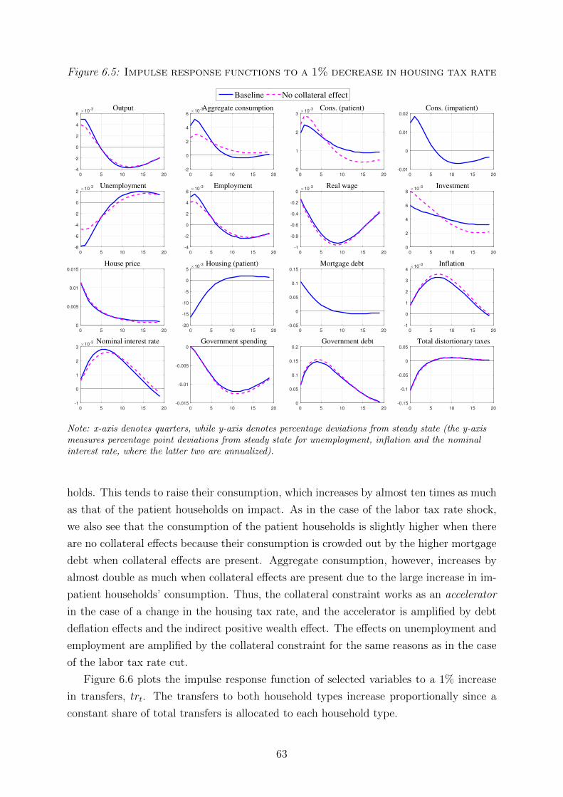
Figure 6.5: Impulse response functions to a 1% decrease in housing tax rate

0

0

Baseline No collateral effect

0 5 10 15 20

-4

-2

0

2

4

6×10

-3 Output

0 5 10 15 20

-2

0

2

4

6×10

-3 Aggregate consumption

0 5 10 15 20

0

1

2

3×10

-3 Cons. (patient)

0 5 10 15 20

-0.01

0

0.01

0.02

Cons. (impatient)

0 5 10 15 20

-8

-6

-4

-2

0

2×10

-3 Unemployment

0 5 10 15 20

-4

-2

0

2

4

6×10

-3 Employment

0 5 10 15 20

-1

-0.8

-0.6

-0.4

-0.2

0×10

-3 Real wage

0 5 10 15 20

0

2

4

6

8×10

-3 Investment

0 5 10 15 20

0

0.005

0.01

0.015

House price

0 5 10 15 20

-20

-15

-10

-5

0

5×10

-3 Housing (patient)

0 5 10 15 20

-0.05

0

0.05

0.1

0.15

Mortgage debt

0 5 10 15 20

-1

0

1

2

3

4×10

-3 Inflation

0 5 10 15 20

-1

0

1

2

3×10

-3 Nominal interest rate

0 5 10 15 20

-0.015

-0.01

-0.005

0

Government spending

0 5 10 15 20

0

0.05

0.1

0.15

0.2

Government debt

0 5 10 15 20

-0.15

-0.1

-0.05

0

0.05

Total distortionary taxes

Note: x-axis denotes quarters, while y-axis denotes percentage deviations from steady state (the y-axismeasures percentage point deviations from steady state for unemployment, inflation and the nominalinterest rate, where the latter two are annualized).

holds. This tends to raise their consumption, which increases by almost ten times as much

as that of the patient households on impact. As in the case of the labor tax rate shock,

we also see that the consumption of the patient households is slightly higher when there

are no collateral effects because their consumption is crowded out by the higher mortgage

debt when collateral effects are present. Aggregate consumption, however, increases by

almost double as much when collateral effects are present due to the large increase in im-

patient households’ consumption. Thus, the collateral constraint works as an accelerator

in the case of a change in the housing tax rate, and the accelerator is amplified by debt

deflation effects and the indirect positive wealth effect. The effects on unemployment and

employment are amplified by the collateral constraint for the same reasons as in the case

of the labor tax rate cut.

Figure 6.6 plots the impulse response function of selected variables to a 1% increase

in transfers, trt. The transfers to both household types increase proportionally since a

constant share of total transfers is allocated to each household type.

63

Figure 6.6: Impulse response functions to a 1% increase in transfers

0

0

Baseline No collateral effect

0 5 10 15 20

-0.01

-0.005

0

0.005

0.01

Output

0 5 10 15 20

-5

0

5

10×10

-3 Aggregate consumption

0 5 10 15 20

0

1

2

3

4

5×10

-3 Cons. (patient)

0 5 10 15 20

-0.01

0

0.01

0.02

0.03

0.04

Cons. (impatient)

0 5 10 15 20

-15

-10

-5

0

5×10

-3 Unemployment

0 5 10 15 20

-5

0

5

10×10

-3 Employment

0 5 10 15 20

-2

-1.5

-1

-0.5

0×10

-3 Real wage

0 5 10 15 20

0

0.005

0.01

0.015

Investment

0 5 10 15 20

0

2

4

6×10

-3 House price

0 5 10 15 20

-20

-15

-10

-5

0

5×10

-3 Housing (patient)

0 5 10 15 20

-0.05

0

0.05

0.1

Mortgage debt

0 5 10 15 20

0

2

4

6×10

-3 Inflation

0 5 10 15 20

0

2

4

6×10

-3 Nominal interest rate

0 5 10 15 20

-0.02

-0.015

-0.01

-0.005

0

Government spending

0 5 10 15 20

0

0.05

0.1

0.15

0.2

0.25

Government debt

0 5 10 15 20

0

0.005

0.01

0.015

0.02

0.025

Total distortionary taxes

Note: x-axis denotes quarters, while y-axis denotes percentage deviations from steady state (the y-axismeasures percentage point deviations from steady state for unemployment, inflation and the nominalinterest rate, where the latter two are annualized).

An increase in transfers initially increases output, consumption, employment, invest-

ment, house prices, inflation and the interest rate, while unemployment and real wages

fall.

The increase in transfers is equivalent to a persistent negative shock to lump-sum

taxes. This positive wealth effect increases consumption and shifts the labor supply curve

of both households inwards. Labor and capital demand increases due to the increase in

aggregate demand, which increases investment and employment. Although the increase

in transfers is non-distortionary by itself, the households expect the tax rates on capital,

labor and consumption to increase due to the higher government debt and output, while

they expect government spending to decrease.

Inflation increases and the central bank increases the interest rate. The expected real

interest rate decreases on impact but this is due to the high degree of interest rate smooth-

ing. This further stimulates the increase in consumption due to intertemporal substitution

effects. Again, real wages decrease because of the high degree of wage stickiness, while

64

the labor unions’ decrease the wage markup, which lowers unemployment.

House prices increase as the marginal utility of patient households’ consumption de-

creases due to their higher consumption. The increase in house prices as well as the lower

expected real interest rate increases mortgage debt through the collateral constraint, which

further stimulates the consumption of the impatient households. The real value of mort-

gage debt is also reduced on impact due to the increase inflation. Thus, the collateral

constraint works as an accelerator that is further amplified by debt deflation and the

indirect positive wealth effect in the case of an increase in transfers. Similar to the case of

the cut in the housing tax rate, we see that unemployment falls more on impact because

of the collateral constraint.

6.2 Fiscal multipliers

The analysis above of the impulse response functions to the six fiscal instrument illustrated

that the effect of the collateral constraint on a fiscal expansion depends on the fiscal

instrument used: the collateral constraint works as an accelerator in the case of a fiscal

expansion using the labor tax rate, transfers or the housing tax rate, while it works as

a decelerator when the fiscal expansion works through government spending, the capital

tax rate or the VAT rate.

We now evaluate the stimulative effects of fiscal policy by computing both impact

multipliers and present value multipliers for a shock to a fiscal instrument Ft:

Impact multiplier k periods ahead =Et∆Yt+k

∆Ft≈ EtYt+k

Ft· YF

Present value multiplier k periods ahead =Et∑k

i=0 (1 + r)−i ∆Yt+i

Et∑k

i=0 (1 + r)−i ∆Ft+i≈ Et

∑ki=0(1 + r)−iYt+i

Et∑k

i=0(1 + r)−iFt+i· YF

Hence, the government spending multiplier measures the change in the level of output for

a change in the level of government spending, while the transfers multiplier measures the

change in the level of output for a change in the level of transfers. The tax multipliers are

measured in terms of the change in total tax revenue from distortionary taxes following

Zubairy (2014) such that the tax multipliers measure the change in the level of output for

a change in the level of total tax revenue from distortionary taxes as a result of a shock

to the tax rate of interest.

The impact multiplier does not account for the dynamic feedback effects from an ini-

tial fiscal policy shock to the fiscal instruments themselves through the fiscal policy rules.

Instead, the present value multiplier is more appropriate in our setting as the subsequent

endogenous changes in fiscal policy after a shock are included in the multiplier. Moreover,

it is important to look at the long term consequences of fiscal policy, which impact mul-

tipliers are inadequate for as argued by Uhlig (2010). This is especially relevant for the

65

government spending multiplier in our model since the gradual increase in distortionary

taxation after a positive government spending shock causes output to fall below steady

state after 8 quarters. The present value multiplier, however, does not account for the

total change in the government’s primary deficit after a fiscal expansion (e.g. the govern-

ment spending multiplier does not measure the attenuating effect on the primary deficit

from a higher tax revenue following the fiscal expansion).

The posterior means of the present value multipliers are presented for government

spending, transfers and the four tax rates in table 4 at four different horizons. The poste-

rior fiscal multipliers were computed by drawing 25,000 random parameter vectors from

the 400,000 post-burnin posterior draws generated by the Metropolis-Hastings algorithm,

simulating the model for each parameter vector and calculating the fiscal multipliers for

each of these simulations. Afterwards the posterior means and probability intervals of

the fiscal multipliers were computed as their sample equivalents as described in section

5. The size of the tax shocks were normalized such that they generate a 1 % decrease

in total tax revenues on impact following Zubairy (2014).29 The impact multipliers are

shown in table 9 in appendix D but not discussed.

Table 4: Present value multipliers for output

1 quarter 4 quarters 12 quarters 20 quarters

PV∆Yt+k

PV∆Gt+k0.94 0.79 0.45 0.12

[0.83, 1.06] [0.67, 0.92] [0.37, 0.54] [0.04, 0.20]PV∆Yt+k

−PV∆TCt+k

0.62 0.84 0.54 0.02

[0.50, 0.76] [0.71, 0.99] [0.42, 0.67] [−0.17, 0.19]PV∆Yt+k

−PV∆TWt+k

0.25 0.37 0.14 -0.39

[0.18, 0.34] [0.28, 0.47] [0.03, 0.24] [−0.58,−0.22]PV∆Yt+k

−PV∆TKt+k

0.25 0.30 1.32 3.00

[−0.03, 0.45] [0.07, 0.48] [0.66, 2.24] [0.92, 5.21]PV∆Yt+k

−PV∆THt+k

0.21 0.31 0.01 -0.60

[0.17, 0.27] [0.24, 0.38] [−0.10, 0.38] [−0.86,−0.39]PV∆Yt+k

PV∆TTrt+k

0.29 0.36 0.12 -0.18

[0.20, 0.40] [0.28, 0.47] [0.04, 0.21] [−0.28,−0.07]

Note: The reported values are the means of the present value multipliers calculated for simulations ofthe model for 25,000 parameter vectors randomly drawn from the draws generated by the MH algorithm.The 5% and 95% percentiles of the posterior distribution are reported below in brackets.

The posterior mean government spending multiplier is slightly less than one on im-

pact, which lies within the range of estimated multipliers typically found in the empirical

literature discussed in section 2. Hence, although consumption and investment does de-

29A shock to one of the tax rates will not affect the other tax rates on impact since the fiscal instrumentsrespond to lagged output and government debt in our specification of the fiscal policy rules. However,the other tax rates will change in the subsequent periods through the effect of the initial shock on outputand government debt, which affects tax revenues.

66

crease after an increase in government spending, the crowding out effects are limited and

an increase in government spending will increase GDP by almost the same dollar amount

on impact. The stimulative effects are, however, rather short-lived. The multiplier is

about halved after 3 years and is only 0.1 after 5 years. Our estimate of the impact

multiplier is close to the estimate of 1.07 by Zubairy (2014) but substantially higher than

the multiplier of 0.64 in the RBC model by Leeper et al. (2010). Leeper et al. (2015) find

a higher impact multiplier of 1.26 in their model, wherein government spending enters

the households’ utility function. Both Zubairy (2014) and Leeper et al. (2015) obtain

multipliers larger than one since their models are able to produce a positive response of

consumption to government spending shocks. Similar to those authors, we find that the

multiplier decreases monotonically across the horizon. Many of the studies reviewed in

section 2, however, find that the multiplier is hump-shaped and does not peak on impact.

Similar to Zubairy (2014) and Leeper et al. (2010), we find that taxes typically become

stimulative over the medium run in comparison to a boost to government spending. The

posterior mean consumption tax multiplier is 0.62 on impact but increases to 0.84 after

1 year. This is due to the hump-shaped response of output but also because the initial

increase in government debt as well as the increase in output cause the remaining fiscal

instruments to counteract the consumption tax shock and increase tax revenues. This

tends to improve the initial deterioration in government’s budget balance and increase

the multiplier.

Capital taxes are especially stimulative over a longer horizon. The posterior mean

impact multiplier is small – around 0.25 – while it increases to around 3 after 5 years: an

initial shock to capital taxes, which causes total tax revenue to decrease one percent on

impact, will increase the present value of output by 3 times as much as the present value

of total taxes decreases over the next 5 years. This large stimulative effect of a capital

tax cut over a longer horizon is similar to what is found by Leeper et al. (2010). We also

saw in figure 6.4 that a reduction in capital taxes are mostly stimulative over the medium

run as investment and consumption gradually increase following the shock.

Neither the posterior mean of the labor tax multiplier nor the housing tax multiplier is

very large. They are both around 1/4 on impact, increase slightly to 1/3 after 1 year and

actually become negative after 5 years. In comparison, Zubairy (2014) finds that labor tax

cuts become more stimulative than capital tax cuts after 3 years: her posterior estimate

of the labor tax multiplier is 0.85 over a 5 year horizon, while the posterior estimate of

the capital tax multiplier is 0.46. Our results are more in line with those of Leeper et al.

(2010) who also find that capital tax cuts are stimulative than labor tax cuts over a long

horizon. Depending on the financing strategy of the government, they also find that the

labor tax multiplier can change sign over a longer horizon and become negative. The

size of the posterior mean of the transfers multiplier is close to that of the labor tax and

housing tax multipliers. Similarly, it has a hump-shaped form and becomes negative at a

67

5 year horizon.

In summary, government spending is the most stimulative of the fiscal instruments

in the short run, while cuts to capital taxes are most stimulative in the long run when

looking at the effect on output. The 90 % Bayesian credibility intervals are rather large

at longer horizons though, especially for the capital tax multiplier. This widening of the

Bayesian credibility intervals as the multiplier horizon increases is consistent with the

results of Zubairy (2014).

We have also calculated the present value multipliers for consumption and investment,

which are presented in tables 5 and 6.

Table 5: Present value multipliers for consumption

1 quarter 4 quarters 12 quarters 20 quarters

PV∆Ct+k

PV∆Gt+k-0.14 -0.20 -0.34 -0.50

[−0.18,−0.09] [−0.26,−0.14] [−0.39,−0.29] [−0.55,−0.44]PV∆Ct+k

−PV∆TCt+k

0.58 0.87 1.16 1.32

[0.49, 0.67] [0.78, 0.97] [1.03, 1.31] [1.11, 1.59]PV∆Ct+k

−PV∆TWt+k

0.15 0.28 0.45 0.53

[0.11, 0.20] [0.22, 0.35] [0.37, 0.53] [0.41, 0.66]PV∆Ct+k

−PV∆TKt+k

-0.17 -0.21 0.03 0.20

[−0.26,−0.11] [−0.29,−0.15] [−0.21, 0.29] [−0.11, 1.14]PV∆Ct+k

−PV∆THt+k

0.11 0.21 0.33 0.38

[0.09, 0.14] [0.17, 0.25] [0.27, 0.25] [0.25, 0.52]PV∆Ct+k

PV∆TTrt+k

0.17 0.26 0.28 0.26

[0.12, 0.23] [0.21, 0.33] [0.23, 0.33] [0.19, 0.33]

Note: The reported values are the means of the present value multipliers calculated for simulations ofthe model for 25,000 parameter vectors randomly drawn from the draws generated by the MH algorithm.The 5% and 95% percentiles of the posterior distribution are reported below in brackets.

68

Table 6: Present value multipliers for investment

1 quarter 4 quarters 12 quarters 20 quarters

PV∆It+k

PV∆Gt+k-0.14 -0.18 -0.27 -0.36

[−0.20,−0.09] [−0.23,−0.13] [−0.32,−0.22] [−0.41,−0.30]PV∆It+k

−PV∆TCt+k

-0.10 -0.17 -0.33 -0.42

[−0.14,−0.07] [−0.21,−0.12] [−0.41,−0.25] [−0.60,−0.27]PV∆It+k

−PV∆TWt+k

0.04 0.05 0.13 0.25

[0.02, 0.07] [0.02, 0.09] [0.07, 0.19] [0.14, 0.37]PV∆It+k

−PV∆TKt+k

-0.18 -0.14 0.31 1.71

[−0.30,−0.11] [−0.23,−0.08] [0.10, 0.61] [0.61, 2.20]PV∆It+k

−PV∆THt+k

0.05 0.08 0.23 0.42

[0.03, 0.07] [0.05, 0.11] [0.17, 0.11] [0.29, 0.59]PV∆It+k

PV∆TTrt+k

0.05 0.06 0.08 0.11

[0.02, 0.09] [0.03, 0.09] [0.04, 0.12] [0.06, 0.17]

Note: The reported values are the means of the present value multipliers calculated for simulations ofthe model for 25,000 parameter vectors randomly drawn from the draws generated by the MH algorithm.The 5% and 95% percentiles of the posterior distribution are reported below in brackets.

The present value multipliers on consumption and investment indicate what drives the

multipliers for output.30 Investment and consumption crowd out the government spend-

ing shock but this is counteracted by an increase in utilization rate. Not surprisingly,

consumption drives the output multiplier after a consumption tax cut, while investment

crowds out the tax cut due to the preferable tax treatment of consumption goods. Con-

sumption especially adds to the multiplier after a labor tax cut but investment also in-

creases the multiplier. The multiplier becomes negative, however, in the medium run as

government spending and the utilization rate decreases. Investment is the main driver of

the multiplier in the medium run when the capital tax rate is decreased but consump-

tion also crowds in after about 1 year as patient households increase their consumption.

When looking at the housing tax cute, both consumption and investment increases but

consumption seems to contribute most to the multiplier. This is also the case for the

multiplier when looking at the increase in transfers.

6.3 Fiscal multipliers and financial conditions

We now turn our attention to how changes in financial conditions affect fiscal multipliers.

First, we analyze the effects of variations in financial conditions by varying the LTV ratio,

m. Figure 6.7 plots the present value multiplier for output for the six different fiscal

instruments as a function of the LTV ratio, while the remaining parameters are fixed at

their posterior mean values. The multipliers are plotted for the same horizons as in the

30Note that utilization costs and government spending are also included in output such that theirresponses also affect the output multiplier.

69

previous tables.31

Figure 6.7: Fiscal multipliers as a function of the LTV ratio

0

02

1 quarter 4 quarters 12 quarters 20 quarters

0 0.2 0.4 0.6 0.8 1

LTV ratio

0

0.2

0.4

0.6

0.8

1

Government spending multiplier

0 0.2 0.4 0.6 0.8 1

LTV ratio

0

0.2

0.4

0.6

0.8

1

VAT multiplier

0 0.2 0.4 0.6 0.8 1

LTV ratio

-0.5

0

0.5

1

Labor tax multiplier

0 0.2 0.4 0.6 0.8 1

LTV ratio

-1

0

1

2

3

Capital tax multiplier

0 0.2 0.4 0.6 0.8 1

LTV ratio

-1

-0.5

0

0.5

1

Housing tax multiplier

0 0.2 0.4 0.6 0.8 1

LTV ratio

-0.4

-0.2

0

0.2

0.4

0.6

Transfer multiplier

The LTV ratio mainly affects the multiplier through its effect on the consumption of

impatient households, which is because the LTV ratio determines how much a change in

house prices alters the borrowing capacity of the impatient households. If house prices fall

following a fiscal policy shock then the borrowing capacity of the impatient households

is reduced more if the LTV ratio is higher. Thus, the impatient households are forced

to both borrow and consume less following a decrease in house prices when the collateral

constraint binds, while the reverse is true if house prices increase. Consequently, the effect

of a higher LTV ratio on the fiscal multiplier is not uniform across fiscal instruments since

the instruments do not have an uniform impact on house prices, and we also see in figure

6.7 that the effect on the fiscal multiplier of a change in the LTV ratio is determined by

how house prices react to the fiscal shock.

The net worth of the impatient households – which is their asset holdings less debt –

is also affected by the LTV ratio:

nw′t = qth′t −

(1 + rt−1)bt−1

1 + πt= qt

(h′t −mξmt−1h

′t−1

)(6.3)

31The size of the multipliers in this section can deviate from the size of the multipliers presented inthe previous section. This is because the multipliers in this section are the multiplier calculated withparameters set at their posterior means, while those in the previous section are the posterior means ofthe multipliers. The difference between the posterior mean multiplier and the multiplier at the posteriormean is especially prominent for the capital tax multiplier at longer horizons.

70

If the LTV ratio increases, it means that the impatient households can accumulate more

houses but it also increases their leverage, which tends to decrease net worth. Indeed,

the steady state net worth, qh′(1 −m), approaches zero as m tends to one. As a shown

by Andres et al. (2015), the consumption function for the impatient households is ap-

proximately a linear and positive function of current labor income and net worth. Thus,

as leverage increases and net worth falls, the consumption of the impatient households

depends more on their current labor income.

A higher LTV ratio reduces the effect of a positive government spending shock on

output. This is because the decrease in house prices following the increase in government

spending forces the impatient households to consume even less if the LTV ratio is higher.

Debt deflation effects partially offset this, however, because mortgage debt will be higher

in steady state when the LTV ratio is higher. The reduction in the multiplier is only

significant for a short horizon and a relatively high LTV ratio (above 0.8).

Conversely, a higher LTV ratio increases the fiscal multiplier for a negative shock to

labor taxes or housing taxes. This is because a decrease in either labor or housing taxes

increases house prices, which causes mortgage debt and consumption of the impatient

households to increase through the collateral constraint. A higher LTV ratio increases

borrowing capacity and thereby consumption and output even more. In addition, debt

deflation effects reinforce the collateral constraint effect in both cases, which also tends

to increase the multiplier as the LTV ratio increases. For similar reasons, the multiplier

for lump-sum transfers is also an increasing function of the LTV ratio.

The capital tax multiplier is reduced as the LTV ratio increases. Similar to the gov-

ernment spending shock, this is because of the deceleration effects from the collateral

constraint is amplified. Debt inflation effects will also tend to intensify the deceleration.

The effect of the LTV ratio on the multiplier for the VAT rate is small and ambiguous.

Since house prices seem to be a main driver of the collateral constraint channel, this small

effect is likely because house prices do not move much following a shock to this fiscal

instrument, while debt deflation counteracts the effect of the collateral constraint.

Next, we analyze how the share of collateral constrained households affects the fiscal

multiplier by plotting the fiscal multipliers as a function of the share of patient households,

µ, in figure 6.8. The remaining parameters are kept at their posterior mean values.

71

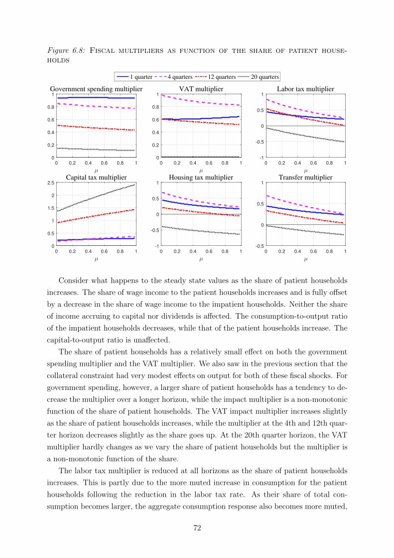
Figure 6.8: Fiscal multipliers as function of the share of patient house-holds

0

02

1 quarter 4 quarters 12 quarters 20 quarters

0 0.2 0.4 0.6 0.8 1

µ

0

0.2

0.4

0.6

0.8

1

Government spending multiplier

0 0.2 0.4 0.6 0.8 1

µ

0

0.2

0.4

0.6

0.8

1

VAT multiplier

0 0.2 0.4 0.6 0.8 1

µ

-1

-0.5

0

0.5

1

Labor tax multiplier

0 0.2 0.4 0.6 0.8 1

µ

0

0.5

1

1.5

2

2.5

Capital tax multiplier

0 0.2 0.4 0.6 0.8 1

µ

-1

-0.5

0

0.5

1

Housing tax multiplier

0 0.2 0.4 0.6 0.8 1

µ

-0.5

0

0.5

1

Transfer multiplier

Consider what happens to the steady state values as the share of patient households

increases. The share of wage income to the patient households increases and is fully offset

by a decrease in the share of wage income to the impatient households. Neither the share

of income accruing to capital nor dividends is affected. The consumption-to-output ratio

of the impatient households decreases, while that of the patient households increase. The

capital-to-output ratio is unaffected.

The share of patient households has a relatively small effect on both the government

spending multiplier and the VAT multiplier. We also saw in the previous section that the

collateral constraint had very modest effects on output for both of these fiscal shocks. For

government spending, however, a larger share of patient households has a tendency to de-

crease the multiplier over a longer horizon, while the impact multiplier is a non-monotonic

function of the share of patient households. The VAT impact multiplier increases slightly

as the share of patient households increases, while the multiplier at the 4th and 12th quar-

ter horizon decreases slightly as the share goes up. At the 20th quarter horizon, the VAT

multiplier hardly changes as we vary the share of patient households but the multiplier is

a non-monotonic function of the share.

The labor tax multiplier is reduced at all horizons as the share of patient households

increases. This is partly due to the more muted increase in consumption for the patient

households following the reduction in the labor tax rate. As their share of total con-

sumption becomes larger, the aggregate consumption response also becomes more muted,

72

which reduces the multiplier. The difference in the consumption pattern between the two

types of households also explains why the housing tax multiplier decreases as the share of

patient households falls. When the negative housing tax shock increases house prices, the

increase in the value of collateral boosts the consumption of the impatient households.

Hence, the increase in aggregate consumption is larger when more households are impa-

tient. Similar effects on the impatient households’ consumption pattern explains why the

transfer multiplier decreases with the share of patient households.

The capital tax rate multiplier increases with the share of patient households and

this is especially the case over longer horizons, where the capital tax multiplier over 20

quarters approaches 2.5 as the share of patient households tends to one. This is because

the stimulative effects of the reduction in the capital tax rate are largest over the medium

run through the dynamic effects on investment and consumption. While consumption

and employment of both household types fall on impact, investment as well as patient

households’ consumption gradually increase above steady state. As the consumption-to-

output ratio of the patient households increases with the share of patient households, this

medium run impact from higher consumption becomes larger.

7 Variance decomposition

We do a forecast error variance decomposition of some of the endogenous variables to

quantify how much each shock – and especially fiscal policy shocks – contributes to the

variance of these variables. A forecast error variance decomposition quantifies how much

each shock contributes to the mean squared error of the k-period-ahead forecast of the

state vector St (Hamilton, 1994):

MSE (St+k) = E[(St+k − Et [St+k]) (St+k − Et [St+k])

′](7.1)

The mean squared error above can be written as a weighted sum of the variances by

using the moving average representation of the model and exploiting that the shocks are

orthogonal. Thus, we can calculate the contribution of each shock to the forecast error

variance as the shock’s share of this weighted sum of variances. These contributions are

reported for different forecast horizons in table 7. We only analyze shocks included in the

estimated model so the housing tax rate shock has been turned off.

73

Table 7: Variance decomposition

PM IP LP CC WM HP P MP GS TR WT VAT CT

After 1 quarterOutput 1 2 0 0 48 0 8 40 1 0 0 0 0Consumption 1 24 0 1 26 0 3 43 0 0 0 0 0- of patient 0 45 0 0 18 0 1 35 0 0 0 0 0- of impatient 3 0 0 14 31 3 8 39 0 0 1 0 0Government spending 0 0 0 0 0 0 0 0 100 0 0 0 0Investment 1 3 0 0 61 0 2 32 0 0 0 0 0Mortgage debt 3 1 0 26 10 43 2 15 0 0 0 0 0Inflation 91 0 0 0 5 0 4 0 0 0 0 0 0Unemployment 3 2 3 1 34 0 24 32 0 0 0 0 0House prices 1 1 0 0 8 73 1 16 0 0 0 0 0VAT rate 0 0 0 0 0 0 0 0 0 0 0 100 0Capital tax rate 0 0 0 0 0 0 0 0 0 0 0 0 100Labor tax rate 0 0 0 0 0 0 0 0 0 0 100 0 0Transfers 0 0 0 0 0 0 0 0 0 100 0 0 0Government debt 4 1 0 0 23 1 15 19 8 2 19 1 6

After 10 quartersOutput 7 2 0 0 52 1 7 32 1 0 0 0 0Consumption 6 21 0 1 26 0 6 38 1 0 1 0 0- of patient 9 40 0 0 16 0 9 25 1 0 0 0 0- of impatient 2 0 0 8 37 4 7 38 0 0 2 0 0Government spending 0 0 0 0 2 0 1 1 92 0 2 0 1Investment 4 5 0 0 69 0 4 16 0 0 0 0 0Mortgage debt 2 2 0 30 11 36 3 16 0 0 1 0 0Inflation 17 0 0 0 70 0 12 0 0 0 0 0 0Unemployment 4 2 5 0 40 0 19 28 0 0 0 0 0House prices 3 4 0 0 8 70 3 12 0 0 0 0 0VAT rate 0 0 0 0 4 0 2 4 1 0 1 87 0Capital tax rate 1 0 0 0 6 0 4 5 4 0 3 0 76Labor tax rate 2 0 0 0 12 0 3 7 3 0 71 0 1Transfers 0 0 0 0 1 0 0 1 0 96 0 0 0Government debt 3 1 0 0 46 0 6 31 6 1 5 0 1

After 40 quartersOutput 3 1 0 0 77 0 5 13 0 0 0 0 0Consumption 2 5 0 0 79 0 4 10 0 0 0 0 0- of patient 2 8 0 0 80 0 4 5 0 0 0 0 0- of impatient 2 0 0 8 53 3 6 25 1 0 1 0 0Government spending 4 0 0 0 31 0 7 13 38 1 4 0 1Investment 4 7 0 0 65 0 9 14 0 0 0 0 0Mortgage debt 2 2 0 31 12 35 3 15 0 0 0 0 0Inflation 2 0 0 0 96 0 2 0 0 0 0 0 0Unemployment 2 1 3 0 71 0 10 13 0 0 0 0 0House prices 1 2 0 0 57 31 3 5 0 0 0 0 0VAT rate 3 0 0 0 41 0 5 9 4 0 2 36 0Capital tax rate 4 0 0 0 41 0 8 11 6 0 3 0 27Labor tax rate 4 0 0 0 30 0 8 10 6 0 40 0 1Transfers 1 0 0 0 7 0 2 2 2 85 1 0 0Government debt 4 0 0 0 74 0 6 11 3 0 1 0 0

Abbreviations: PM: Price markup; IP: Intertemporal preference; LP: Labor preference; CC: Collateralconstraint; WM: Wage markup; HP: Housing preference; P: Productivity; MP: Monetary policy; GS:Government spending; TR: Transfers; WT: Labor tax rate; VAT: Consumption tax rate; CT: Capitaltax rate.

74

None of the fiscal shocks contribute considerably to the variance of the components

of GDP (except to the variance of government spending of course). Instead, the wage

markup and the monetary policy shocks contribute to most of the variance of the com-

ponents of GDP at a horizon of both 1 quarter and 10 quarters, while the price markup

and the productivity shocks also contribute a little to the variance of the GDP compo-

nents. The intertemporal preference shock contributes to about 1/5-1/4 of the variance

of consumption at the same horizons. After decomposing the consumption variance into

the two household types, we see that the intertemporal preference shock is only important

for the variance of the patient households’ consumption. This is because this shock has a

direct effect on the consumption pattern of the patient households. Similarly, the shock is

also relatively important for the variance of investment through its effect on their savings

behaviour. The decomposition of consumption variance also reveals that the housing re-

lated shocks – the housing preference and collateral constraint shocks – contribute to the

consumption variance of the impatient households but not that of the patient households.

This is because of the collateral constraint: shocks that affect the collateral constraint

of the impatient households’ also affect their consumption. Finally, when looking at the

40-quarter horizon variance decomposition, the wage markup shock by far contributes to

most of the variance of the GDP components. As mentioned earlier in section 5.5, this is

caused by the shock’s high autocorrelation component.

Turning to the housing market variables, the housing preference shock contributes to

a considerable share of the variance of both house prices and mortgage debt at the 1th,

10th and 40th quarter horizons. The collateral constraint shock, in comparison, explains

a large share of the variance of mortgage debt and contributes to none of the variance of

house prices. This is not only because the posterior mean of the variance of the housing

preference shock is large compared to that of other shocks but also because housing

preference shocks affect house prices directly by shifting both households types’ housing

demand curves and thereby also affecting mortgage debt through the collateral constraint.

Conversely, the collateral constraint shock shifts the impatient households’ demand for

debt since their collateral constraint is binding, while only shifting the housing demand

curve of impatient households. House prices are pinned down by the patient households’

shadow value of consumption, however, so the effect of changes in LTV ratio on house

prices is small. Thus, house price fluctuations are mostly driven by housing preference

shocks and not exogenous shocks to financial conditions according to the model (Iacoviello

and Neri (2010) discuss this property of the model in their appendix). The monetary policy

shock also explains about 15 per cent of the variance of both house prices and mortgage

debt over the short horizon. Wage markup shocks explain most of the variance of house

prices at the 40-quarter horizon but housing preference shocks still contribute to about

a third of the forecast error variance. The collateral constraint, housing preference and

monetary policy shocks still contribute to a large share of the variance in mortgage debt

75

at the 40-quarter horizon. This is because each of these three shocks directly influence

mortgage debt through the collateral constraint. Finally, fiscal shocks explain close to

none of the variance of the housing market variables at any forecast horizon.

The variance of inflation is mostly driven by the price markup shock at the 1-quarter

horizon. This is not surprising since it has a direct effect on inflation through the Phillips

curve. As the forecast horizon increases, the productivity shock and the wage markup

shock become more important with the wage markup shock dominating at the 40-quarters

forecast horizon. Both of these shocks affect prices through their effect on the wholesale

firms’ marginal costs. The variance of unemployment is mostly driven by the wage markup

shock directly through the wage Phillips curve, while the productivity and monetary policy

shocks each contribute to about a tenth of the variance.

The variances of the fiscal instruments themselves are mostly explained by their own

shock component at the 10-quarter horizon (at the 1-quarter they are exclusively driven

by their own shock component due to the backward-looking fiscal policy rules). This is

because all of the instruments are persistent and do not react too strongly to debt and

output. Shocks that are important determinants of output and government debt – the

wage markup and monetary policy shocks – also explain some of the variance in the fiscal

instruments through the fiscal policy rules. Relative to the other fiscal instruments, the

variance of transfers is still predominately explained by its own shock at the 40th quarter

horizon. This is mostly because the shock has a relatively high standard deviation. Finally,

the government spending shock explains some of the variance of the tax rates at both the

10th and 40th quarter horizon through its persistent effect on government debt.

Table 7 reveals that the wage markup shock is by far the most important driver of the

forecast error variance of the endogenous variables at longer horizons. This is because this

shock is very persistent. Both Smets and Wouters (2007) and Galı et al. (2012) also find

that the shock is highly persistent with a posterior mean for the autocorrelation parameter

estimated as 0.96 and 0.98 respectively (Iacoviello and Neri (2010) do not include a wage

markup shock in their model). Hence, the shock also explains a large share of the forecast

error variance at long horizons in their models. The half-time of their wage markup

process, however, is still a lot lower than ours so it does not dominate the variance of the

endogenous variables to the same degree in their models.32

To get an idea about the effects of the wage markup autocorrelation parameter on

the variance decomposition, we have performed the variance decomposition for the GDP

components at the 40th quarter horizon for different values of ρw. The results are shown

in table 8.

32The half-time of the wage markup shock process is about 17 and 34 quarters at the posterior meanestimates of Smets and Wouters (2007) and Galı et al. (2012) respectively. The half-time at our posteriormean estimate is about 230 quarters.

76

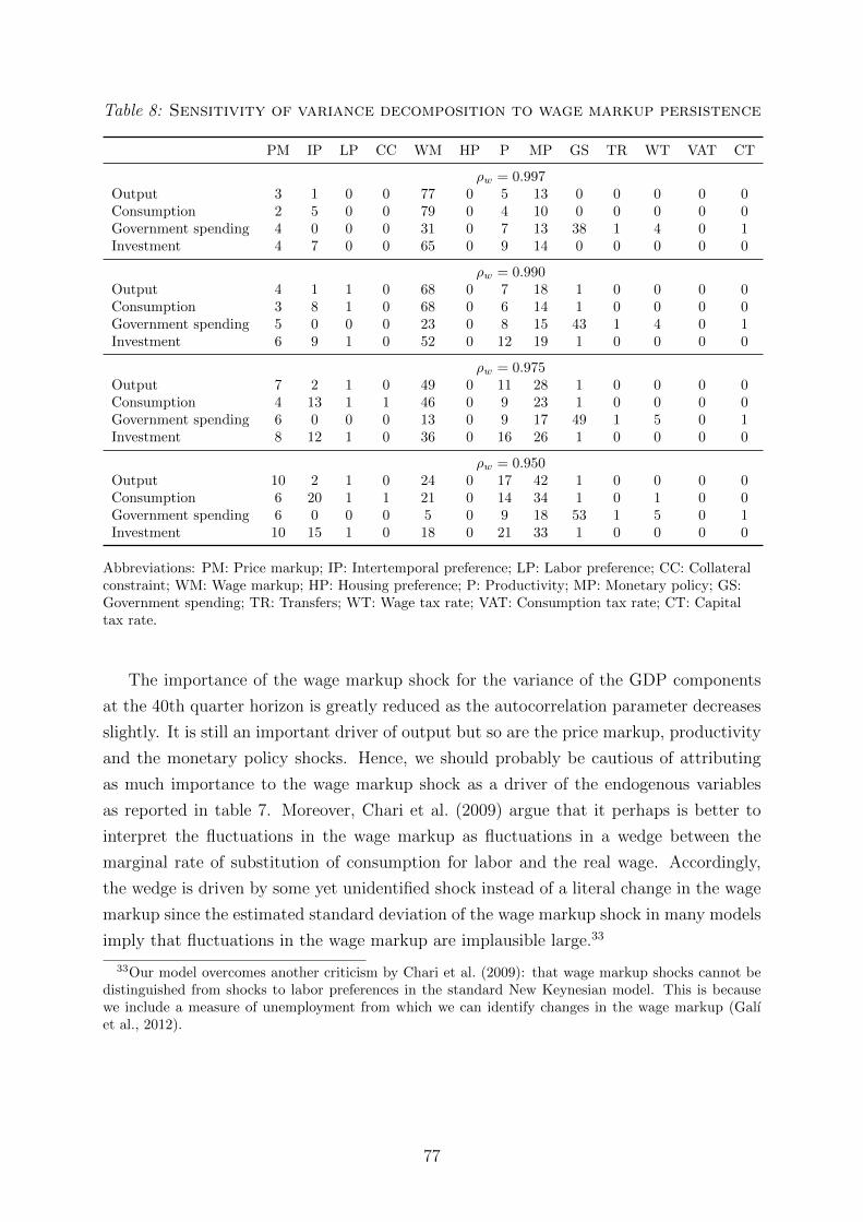
Table 8: Sensitivity of variance decomposition to wage markup persistence

PM IP LP CC WM HP P MP GS TR WT VAT CT

ρw = 0.997Output 3 1 0 0 77 0 5 13 0 0 0 0 0Consumption 2 5 0 0 79 0 4 10 0 0 0 0 0Government spending 4 0 0 0 31 0 7 13 38 1 4 0 1Investment 4 7 0 0 65 0 9 14 0 0 0 0 0

ρw = 0.990Output 4 1 1 0 68 0 7 18 1 0 0 0 0Consumption 3 8 1 0 68 0 6 14 1 0 0 0 0Government spending 5 0 0 0 23 0 8 15 43 1 4 0 1Investment 6 9 1 0 52 0 12 19 1 0 0 0 0

ρw = 0.975Output 7 2 1 0 49 0 11 28 1 0 0 0 0Consumption 4 13 1 1 46 0 9 23 1 0 0 0 0Government spending 6 0 0 0 13 0 9 17 49 1 5 0 1Investment 8 12 1 0 36 0 16 26 1 0 0 0 0

ρw = 0.950Output 10 2 1 0 24 0 17 42 1 0 0 0 0Consumption 6 20 1 1 21 0 14 34 1 0 1 0 0Government spending 6 0 0 0 5 0 9 18 53 1 5 0 1Investment 10 15 1 0 18 0 21 33 1 0 0 0 0

Abbreviations: PM: Price markup; IP: Intertemporal preference; LP: Labor preference; CC: Collateralconstraint; WM: Wage markup; HP: Housing preference; P: Productivity; MP: Monetary policy; GS:Government spending; TR: Transfers; WT: Wage tax rate; VAT: Consumption tax rate; CT: Capitaltax rate.

The importance of the wage markup shock for the variance of the GDP components

at the 40th quarter horizon is greatly reduced as the autocorrelation parameter decreases

slightly. It is still an important driver of output but so are the price markup, productivity

and the monetary policy shocks. Hence, we should probably be cautious of attributing

as much importance to the wage markup shock as a driver of the endogenous variables

as reported in table 7. Moreover, Chari et al. (2009) argue that it perhaps is better to

interpret the fluctuations in the wage markup as fluctuations in a wedge between the

marginal rate of substitution of consumption for labor and the real wage. Accordingly,

the wedge is driven by some yet unidentified shock instead of a literal change in the wage

markup since the estimated standard deviation of the wage markup shock in many models

imply that fluctuations in the wage markup are implausible large.33

33Our model overcomes another criticism by Chari et al. (2009): that wage markup shocks cannot bedistinguished from shocks to labor preferences in the standard New Keynesian model. This is becausewe include a measure of unemployment from which we can identify changes in the wage markup (Galıet al., 2012).

77

8 Counterfactual experiments of financing govern-

ment spending

The fiscal sector is relatively simple in many DSGE models. For example, Smets and

Wouters (2007) let government spending follow an exogenous autoregressive process, while

government spending is fully financed by lump-sum taxes within the same period. But as

Baxter and King (1993) emphasize, there are significant differences between the effects of

government spending financed by changes in distortionary tax rates or lump-sum transfers.

In our estimated model, the fiscal sector collects distortionary taxes, issues bonds, uses

resources on government spending and makes lump-sum transfers to household. Govern-

ment spending follows an autoregressive fiscal policy rule and reacts to output and debt,

and expansionary fiscal policies are financed by increasing both tax rates and debt and

decreasing transfers.

In these counterfactual experiment, we examine the implications of including the en-

dogenous distortionary tax policy rules in our model. We focus on the effects on the

transmission of government spending shocks.

8.1 Lump-sum versus distortionary financing

We analyze the implications of including endogenous distortionary tax policy rules by

comparing the estimated model (baseline) with the model with a simplified fiscal sector.

In the simplified fiscal sector, the discretionary tax rates are held constant at their steady

state value, i.e. expansionary government spending is financed by issuing debt and de-

creasing lump-sum transfers, while the revenue from distortionary taxes only depends on

changes in the tax base. Government spending is not endogenous in both models to make

them more comparable. All other parameters are set to their posterior mean value.34

Figure 8.1 plots the impulse response functions of selected variables to a 1% increase in

government spending.35

The transmission of a 1% increase in government spending with endogenous distor-

tionary tax rates was described in detail in section 6.1. Figure 8.1 shows two differences

are worth mentioning. First, output increases more on impact when tax rates are en-

dogenous. Second, when tax rates are endogenous, an increase in government spending

implies an economic expansion in the short run and an economic contraction in the longer

run, whereas the model with a simplified fiscal sector only implies that there is short run

economic expansion and no economic contraction at a longer horizon.

34The model is calibrated such that ρi,y = ρi,b = 0 , ∀ ∈ {g, w, c, k}. ρbtr is kept unchanged. Weexperimented with changing the time profile of lump-sum transfers but this had minimal influence on thetransmission of government spending shocks although Ricardian equivalence does not hold in our modelbecause of distortionary taxes and the collateral constraint.

35See figure D.7 in appendix D for more detailed plots of the impulse response functions.

78

Figure 8.1: Detailed fiscal sector (baseline) versus simplified fiscal sector:Impulse response functions to a 1% increase in government spending

0Baseline Simplified fiscal sector

0 5 10 15 20

-0.1

0

0.1

0.2

Output

0 5 10 15 20

-0.15

-0.1

-0.05

0

Aggregate consumption

0 5 10 15 20

-0.15

-0.1

-0.05

0

Cons. (patient)

0 5 10 15 20

-0.2

-0.15

-0.1

-0.05

0

Cons. (impatient)

0 5 10 15 20

-0.2

-0.15

-0.1

-0.05

0

0.05

Unemployment

0 5 10 15 20

-0.05

0

0.05

0.1

0.15

0.2

Employment

0 5 10 15 20

-0.04

-0.03

-0.02

-0.01

0

Real wage

0 5 10 15 20

-0.4

-0.3

-0.2

-0.1

0

Investment

0 5 10 15 20

-0.15

-0.1

-0.05

0

House price

0 5 10 15 20

-0.05

0

0.05

0.1

0.15

0.2

Housing (patient)

0 5 10 15 20

-1.5

-1

-0.5

0

0.5

Mortgage debt

0 5 10 15 20

0

0.05

0.1

0.15

Inflation

0 5 10 15 20

0

0.05

0.1

0.15

Nominal interest rate

0 5 10 15 20

0

0.5

1

1.5

Government spending

0 5 10 15 20

-0.8

-0.6

-0.4

-0.2

0

Transfers

0 5 10 15 20

-0.1

0

0.1

0.2

0.3

Total distortionary taxes

Note 1: x-axis denotes quarters, while y-axis denotes percentage deviations from steady state (the y-axismeasures percentage point deviations from steady state for unemployment, inflation and the nominalinterest rate, where the latter two are annualized).Note 2: The simplified fiscal sector is defined as ρtr,y = ρi,y = ρi,b = 0 , ∀ ∈ {w, c, k}. All otherparameters are set to their posterior mean values and ρg,y = ρg,b = 0 in both models.

The higher initial output when tax rates are endogenous is due to the households’

anticipation of a future increase in the distortionary tax rates when government spending

increases. As described in section 6.1, the tax rates on labor, capital income and con-

sumption are hump-shaped. They increase in the quarters after the shock to government

spending, but this is insufficient to finance the higher government spending in the first 14

quarters. The future increase in the tax rates will tend to increase current consumption

and investment as the future increase in the VAT rate lowers the relative price of consump-

tion today versus consumption tomorrow, while the future increase in the capital tax rate

will decrease future after-tax return of capital such that the gains of investing today are

higher than tomorrow. These anticipation effects tend to increase current consumption,

investment and utilization of capital such that output increases more on impact compared

to the model with no endogenous tax rates. We found that the capital tax rate is the main

79

driver of these anticipation effects as only shutting off the endogenous responses of the

consumption and labor tax rates lead to a bigger increase in output on impact. However,

if we increase the labor supply elasticities, 1/ϕ and 1/ϕ′, sufficiently – such that labor

supply becomes more responsive to changes in the labor tax rate – then a future increase

in the labor tax rate can also cause current output to increase. Thus, if the labor supply

elasticity is sufficiently high, output will increase more on impact when the labor tax rate

is endogenous.

We now turn to the present value multiplier to study the effect of the endogenous tax

rates on output in the longer run. The present value government spending multiplier for

output in both models is shown in figure 8.2.

Figure 8.2: Detailed fiscal sector (baseline) versus simplified fiscal sector:Present value government spending multiplier for output

0 5 10 15 20 25 30 35 40

Quarters

-0.4

-0.2

0

0.2

0.4

0.6

0.8

1

Pre

sent

val

ue

mult

ipli

er

Baseline Simplified fiscal sector

Note: Simplified fiscal sector is defined as ρtr,y = ρi,y = ρi,b = 0 , ∀ ∈ {w, c, k}. All other parameters areset to their posterior mean values and ρg,y = ρg,b = 0 in both models.

In the short run, the present value multiplier is greater when tax rates are endogenous

compared to the model with a simplified fiscal sector. Over time, the present value

multiplier in the baseline model decreases more, thus becoming negative after 6 years

and converging to -0.38. By contrast, the present value multiplier is strictly positive at

all horizons in the model with a simplified fiscal sector and converges to a level of 0.15.

The reason for the difference in present value multipliers in the short run is the same as

explained above: an anticipation of an increase in distortionary tax rates in the future

tends to increase output on impact.

The aggressive decrease in the present value multiplier over time in the baseline model

is due to the delayed increase in distortionary tax rates. The delayed increase in the tax

rates lowers consumption, labor supply and investment in capital over time. Compared to

the model with a simplified fiscal sector, output decreases more aggressively over time in

the baseline model causing the present value multiplier to decrease and become negative

80

as output undershoots steady state. Hence, while the endogenous tax rates have an

expansionary effect in the short run by front-loading economic activity, they cause the

present value multiplier to become smaller over a longer horizon due to the distortionary

effects of the higher tax rates.

By comparison, the government spending shock only has a short run effect on output

in the model with the simplified fiscal sector. Output increases initially but converges back

to steady state without undershooting. The effect on lump-sum transfers and government

debt are more long-lived than when tax rates are endogenous: transfers decrease for 16

years after the shock to government spending, while government debt also reaches its peak

after 16 years. But the delayed decrease in transfers will not distort consumption, labor

supply and investment as lump-sum transfers have no distortionary effect. When the tax

rates are endogenous, government debt peaks after only 3 to 4 years.

In summary, financing expansionary government spending by a future increase in dis-

tortionary tax rates can cause a short run economic expansion, but an economic contrac-

tion in the longer run. This indicates that the effects of government spending depend

crucially on how government spending is financed; something which other authors have

also pointed out. Andres et al. (2016) find that the anticipation of an increase in the

consumption tax rate in the future increases current consumption and stimulates output.

Thus, due to an anticipation of higher future consumption tax rates, the multiplier is

larger on impact compared to a model, wherein lump-sum transfers react to the govern-

ment spending shock. Andres et al. (2016) do not find, however, that an anticipation of

higher capital and labor tax rates cause output to increase more on impact. We suspect

that this is because the consumption tax rate increases relatively much in their model

following a government spending shock.36 Zubairy (2014) conducts a similar study to

us. She also finds that the present value multiplier decreases significantly over time when

tax rates are endogenous but the multiplier is consistently higher over all horizons in her

model when only lump-sum transfers react to output and government debt. The latter

is contrary to our findings. Baxter and King (1993) examine the effects of a temporary

increase in government spending under different financing strategies. In their RBC model,

the current tax revenue from lump-sum transfers and distortionary income taxes adjust to

current government spending such that the government budget is balanced within each pe-

riod. Hence, the distortionary tax rate will jump when government spending increases, in

constrast to our model where tax rates gradually increase. Thus, Baxter and King (1993)

find that output actually decreases on impact when financed by distortionary taxes be-

36They analyze the effects of the distortionary tax rates on output by turning the tax rate rules on oneby one (i.e. letting one tax rate by endogenous, while holding the other tax rates constant). Moreover,they specify fiscal policy rules for the tax rates that ensures that the adjustment in the deficit is thesame for a given deviation in the ratio of government debt to output. This implies that the consumptiontax rate must adjust relatively much to ensure the same adjustment in the deficit as the other tax ratesbecause the consumption tax rate is only 5 per cent in steady state.

81

cause of strong substitution effects on labor and investment. By contrast, an increase in

government spending announces an eventual increase in future tax rates in our model,

which causes an immediate increase in output.

8.2 Debt versus tax financing

We now evaluate how the government’s commitment to retire debt after an increase in

government spending affect multipliers. Similar to Zubairy (2014), we modify the fiscal

policy rules for the labor, consumption and capital tax rates in the linearized model as:

(8.1)τ itτ i

= ρiτ it−1

τ i+ γ · ρi,bbGt−1 + ρi,yyt−1 + εi,t , ∀i ∈ {w, c, k}

in which γ = 1 corresponds to the estimated model. γ < (>)1 implies that the fiscal

authority is less (more) committed to retire debt and initially let at a greater (lesser) share

of government spending be financed by debt compared to the baseline model. Similar to

the previous study, government spending is not endogenous.37

Figure 8.3 plots the response of government debt over 40 quarters to a 1% increase in

government spending for different values of γ.

Figure 8.3: Response of government debt to a 1% increase in government spendingfor different values of γ

0 5 10 15 20 25 30 35 40

Quarters

0

1

2

3

4

5

6

7

8

%-d

evia

tio

n f

rom

ste

ady

sta

te

γ=0 γ=0.5 γ=1 (baseline) γ=2 γ=3

Note: The expected path for government spending is identical in every simulation (i.e. ρg,b = ρg,y = 0).All other parameters are set to their posterior mean values.

The government debt’s speed of convergence to the steady state is an increasing func-

tion of γ; an increase in γ reflects the government’s greater interest in retiring the debt.

In our estimated model, corresponding to γ = 1, government debt peaks after 3-4 years,

37The fiscal rule for transfers is not modified as the time profile of lump-sum transfers has minimalinfluence on the transmission of the government spending shock.

82

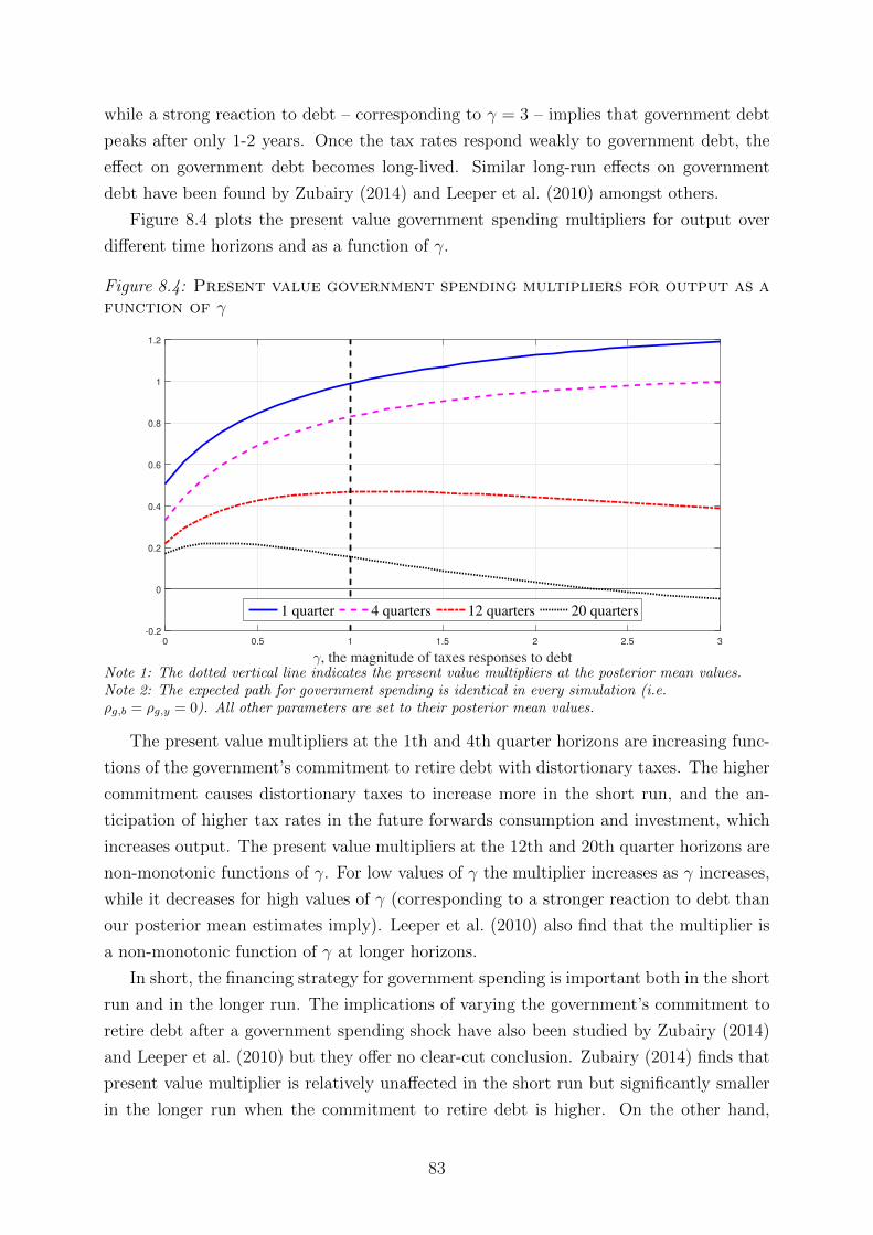
while a strong reaction to debt – corresponding to γ = 3 – implies that government debt

peaks after only 1-2 years. Once the tax rates respond weakly to government debt, the

effect on government debt becomes long-lived. Similar long-run effects on government

debt have been found by Zubairy (2014) and Leeper et al. (2010) amongst others.

Figure 8.4 plots the present value government spending multipliers for output over

different time horizons and as a function of γ.

Figure 8.4: Present value government spending multipliers for output as afunction of γ

0 0.5 1 1.5 2 2.5 3

γ, the magnitude of taxes responses to debt

-0.2

0

0.2

0.4

0.6

0.8

1

1.2

1 quarter 4 quarters 12 quarters 20 quarters

Note 1: The dotted vertical line indicates the present value multipliers at the posterior mean values.Note 2: The expected path for government spending is identical in every simulation (i.e.ρg,b = ρg,y = 0). All other parameters are set to their posterior mean values.

The present value multipliers at the 1th and 4th quarter horizons are increasing func-

tions of the government’s commitment to retire debt with distortionary taxes. The higher

commitment causes distortionary taxes to increase more in the short run, and the an-

ticipation of higher tax rates in the future forwards consumption and investment, which

increases output. The present value multipliers at the 12th and 20th quarter horizons are

non-monotonic functions of γ. For low values of γ the multiplier increases as γ increases,

while it decreases for high values of γ (corresponding to a stronger reaction to debt than

our posterior mean estimates imply). Leeper et al. (2010) also find that the multiplier is

a non-monotonic function of γ at longer horizons.

In short, the financing strategy for government spending is important both in the short

run and in the longer run. The implications of varying the government’s commitment to

retire debt after a government spending shock have also been studied by Zubairy (2014)

and Leeper et al. (2010) but they offer no clear-cut conclusion. Zubairy (2014) finds that

present value multiplier is relatively unaffected in the short run but significantly smaller

in the longer run when the commitment to retire debt is higher. On the other hand,

83

Leeper et al. (2010) find that the present value output multiplier of government spending

decreases in the short run when the commitment to retire debt is high, while the multiplier

in the longer run is a non-monotonic function of γ.

9 Government spending and monetary policy

In this section, we evaluate how the central bank’s monetary policy rule may influence

the stimulative effects of government spending. The monetary policy rule specifies how

the central bank sets the nominal interest rate to stabilize inflation and output, and the

size of the central bank’s reaction is important for the stimulative effects of government

spending as we noted in section 6.1.

An increase in government spending will increase aggregate demand and output, which

put an upward pressure on prices and increase inflation. Both the increase in inflation

and output causes the central bank to increase the nominal interest rate. The size of the

central bank’s increase of the nominal interest rate depends on their monetary policy rule

and determines both the size and direction of the real interest rate. If the increase in

nominal interest rate is greater than the increase in the expected inflation next period,

the expected real interest rate, rt − Et [πt+1], will increase. Conversely, if the increase in

the nominal interest rate is too small, the expected real interest rate will decrease. Due to

intertemporal substitution effects through the Euler equation, an increase in the real in-

terest rate will strengthen the crowding out effect on consumption as current consumption

becomes less attractive compared to future consumption.

To analyze the impact of the monetary policy rule on the stimulative effects of gov-

ernment spending, we compute the present value multiplier for output under different

degrees of interest rate smoothing, φR, and preferences for price and output stability, φπ

and φy. The remaining parameters are set to their posterior mean values. This is shown

in figure 9.1.

The present value multipliers are decreasing functions of both φy and φπ, and for

sufficiently small values of either φy or φπ the impact multiplier is greater than 1. The

reason is that for higher values of φy (φπ), the central bank reacts more aggressively to the

increase in output (inflation) due to the increase in government spending by increasing

the nominal interest rate more. The higher the nominal interest rate is, the higher the

real interest rate is. The higher real interest rate amplifies the crowding out effect of

consumption, and weakens the initial increase in output. In both cases, low values of φy

or φπ implies that the impact multiplier becomes greater than 1, but does neither cause

crowding in of aggregate consumption or an increase in house prices.

84

Figure 9.1: Sensitivity of present value government spending multiplier foroutput to monetary policy parameters

0

02

1 quarter 4 quarters 12 quarters 20 quarters

0.2 0.4 0.6 0.8 1 1.2 1.4 1.6 1.8 2

φy, central bank's preference for output stability

0

0.2

0.4

0.6

0.8

1

1.2

1 1.1 1.2 1.3 1.4 1.5 1.6 1.7 1.8 1.9 2

φπ, central bank's preference for price stability

-0.2

0

0.2

0.4

0.6

0.8

1

1.2

0 0.1 0.2 0.3 0.4 0.5 0.6 0.7 0.8 0.9 1

φR

, degree of interest rate smoothing

-0.2

0

0.2

0.4

0.6

0.8

1

1.2

1.4

1.6

Note: The dotted vertical lines indicate the present value multipliers at the posterior mean values.

The interest rate smoothing parameter, φR, is a weighting parameter between persis-

tence in the nominal interest rate and responsive monetary policy. Two observations are

important here. All four present value multipliers are increasing functions of the interest

rate smoothing parameter, and the difference between the present value multiplier in the

short and long run is an increasing function of the interest rate smoothing parameter as

85

well.

Similar to the cases of less output and inflation stabilization, for a higher interest

rate smoothing parameter the upward pressure on the nominal interest rate is smaller.

For higher degrees of interest rate smoothing, the intertemporal substitution effect will

weaken the crowding out effect of consumption. Actually, for a sufficiently high interest

rate smoothing parameter, the consumption of the households will increase on impact.38

The patient households’ consumption, however, only increases slightly on impact and

quickly falls below steady state. Consequently, house prices also increase on impact but

quickly fall below steady state. Again, the impact multiplier becomes greater than 1 for

small enough values of the interest rate smoothing parameter.

The counterfactual study above emphasizes that government spending is more stimu-

lative under less responsive monetary policy, which is in line with the findings of Zubairy

(2014). When monetary policy is sufficiently accommodative, government spending be-

comes more stimulative, which implies that the impact multiplier becomes greater than

1.

10 Analysis of tax reforms

Our model allows us to quantify how much variations in output and government debt

have contributed to changes in the tax rates compared to exogenous tax shocks. In this

section, we analyze whether major tax reforms during our sample period were driven by

output, government debt or exogenous shocks. We only analyze the shocks to the labor

and capital tax rates.

There were four major tax reforms during our sample period: the tax hike in the

Omnibus Budget Reconciliation Act of 1990 under President George Bush H.W. Bush,

the tax hike in the Omnibus Budget Reconciliation Act of 1993 under President Bill

Clinton, the tax cuts in the Taxpayer Relief Act of 1997 and the Balanced Budget Act

of 1997 under President Bill Clinton and the tax cuts between 2001 and 2003 under

President George W. Bush (Romer and Romer, 2010).39 To get an idea about the causes

of these reforms, we plot the detrended labor and capital tax rates that are used during

estimation of the model together with the smoothed shocks to these rates at the posterior

mean of the parameters in figure 10.1.40 The shocks are multiplied by the steady state tax

rates to calculate the percentage point contribution to the tax rates. In addition, we plot

the effects of output and government debt on the two tax rates implied by the posterior

means of the parameters and the smoothed output and government debt variables at the

38See figure D.8 in appendix D.39We ignore the tax cuts in Tax Reform Act of 1986 and the tax hike in the Omnibus Budget Recon-

ciliation Act of 1987 under Ronald Reagan as both of these fiscal packages were rather small.40A smoothed variable xt is the expected value of that variable given all information, E[xt|yT ], where

yT is the data sample (Hamilton, 1994). The smoothed variables are computed with the Kalman filter.

86

posterior mean of the parameters. These effects have been calculated as follows:

Debt effect on labor tax rate in period t = 0.239 · 0.034 · E[bGt−1|yT

],

Output effect on labor tax rate in period t = 0.239 · 0.272 · E[yt−1|yT ],

Debt effect on capital tax rate in period t = 0.369 · 0.050 · E[bGt−1|yT ],

Output effect on capital tax rate in period t = 0.369 · 0.224 · E[yt−1|yT ]

Figure 10.1: Estimated shocks to the capital and labor tax rates

Note: The solid lines are the actual demeaned tax rates, while the dashed lines are the smoothed taxrate shocks at the posterior means of the parameters. The smoothed tax rate shocks have beenmultiplied by the respective steady state tax rate. Vertical axes are in percentage point deviations fromsteady state.

The correlation between the labor tax rate and its shock is 0.39, while the correlation

between the capital tax rate and its shock is 0.31. Hence, the shocks do some seem to

capture a considerable share of the movements in the tax rates.

The tax reforms can generally be seen in the tax rate series shown in the figure above.

Both of the tax rates increased slightly around the tax hike in 1990. The labor tax rate

gradually increased after the tax hike in 1993, whereas the capital tax rate was almost

87

constant. The tax cut in 1997 is not noticeable in the data. Instead, both tax rates

increased in the late-90s, which could be because we use data for the average tax rates

that have a tendency to rise during an economic boom when the tax system is progressive.

Both the labor tax rate and the capital tax rate decreased significantly – each with about

4-6 percentage points in the course of 2-3 years – after the tax cuts in 2001. From 2004

both tax rates gradually increased although the tax cuts were still in effect and later

extended after the sample period in 2010 (the increase in the tax rates can again be

because of higher economic activity). According to our model, these tax reforms can be

either debt-driven, motivated by output stabilization considerations or exogenous.41

First, we analyze the tax hike in 1990 under Bush Sr. Both of the tax rates increased

slightly around 1990, while output and government debt had an almost neutral effect on

the tax rates. Thus, the model mostly attributes the tax hike to exogenous factors.

Next, we analyze the Clinton tax hike in 1993 as well as the subsequent tax cut in

1997. Government debt was high around 1993, while output was below trend so debt

would cause tax rates to increase and output would cause the rates to decrease. We

see that the labor tax rate shocks were pretty much neutral around the tax hike with

government debt contributing most to the increase in the tax rate. The labor tax rate

shocks only became positive around the turn of the millennium as government debt fell

and output increased. The capital tax rate shock was mostly negative after 1993, which

offset the positive effects of the government debt on the capital tax rate, which only

increased slightly after 1993. The model does not pick up the tax cut in 1997 but as

mentioned above neither does the data. In summary, the model mostly attributes the

Clinton tax hike to endogenous factors, especially government debt, while the later tax

cut is not identified by the model.

The Bush tax cuts abruptly ended the gradually rising tax rates. During the same

period the American economy experienced a short-lived recession. Government debt,

however, was 20-25 per cent below its trend value according to our data, while output was

above trend until 2002. Hence, government debt had a substantial negative effect on the

tax effects on the tax rates, while output had a small but positive effect until 2002 after

which it had a small negative effect. The net effect was negative around the tax cuts.

Meanwhile, both tax rate processes did experience large negative shocks around 2001 and

2002, which indicates that the tax cuts were to some extent exogenously driven.

How does the analysis above stack up with the narrative analysis by Romer and

Romer (2010)? The Romers clearly view the purpose of both the Bush Sr. and Clinton

tax hikes in 1990 and 1993 as deficit reduction. Our analysis attributes the tax hike in

1990 to exogenous shocks but this is likely because of the starting date of our sample

41Our definition of an exogenous change in fiscal policy differs from that of Romer and Romer (2010)due to the fiscal instruments’ reaction to government debt. They treat a debt-driven tax reform asexogenous because it is not motivated by short-run considerations and therefore should be orthogonal tothe business cycle. Such a reform is endogenous in our model.

88

period as government debt increased considerably during the 1980s. Hence, if our sample

period went longer back in time, we would possibly see debt as a driver of the tax hike.

The tax hike in 1993 is mostly attributed to high government debt in the model, while

the exogenous shocks have to drive the increase in tax rates during the late 1990s as

government debt gradually fell. The subsequent tax cuts in 1997 are interpreted as being

driven by spending cuts by the Romers but we do not see these tax cuts in the data nor the

model. The Bush tax cuts are interpreted more carefully by the Romers but mostly viewed

as exogenous. The tax cuts in the Economic Growth and Tax Relief Reconciliation Act of

2001 were largely attributed to ideological reasons but some of them are also attributed to

countercyclical motives. The smaller package of tax cuts in the Job Creation and Worker

Assistance Act of 2002 is attributed to output stabilization motives, especially to offset

adverse macroeconomic shocks from the terrorist attacks of September 11, 2001. Finally,

the tax cuts in the Jobs and Growth Tax Relief Reconciliation Act of 2003 are attributed

to a desire to increase long-run growth (i.e. an exogenous motive). In summary, the model

largely reaches the same conclusion about the Clinton tax hike and the Bush tax cuts as

the narrative analysis by Romer and Romer (2010).

11 Discussion: The response of consumption and house

prices to government spending shocks

The model analyzed in this paper predicts a fall in consumption after a positive govern-

ment spending shock, which is at odds with what is typically found in the SVAR literature

using the Blanchard-Perotti identification scheme. House prices also fall since they are

pinned down by the shadow value of consumption of the patient households. There are

still, however, relatively few empirical studies on the response of house prices to govern-

ment spending as we discussed in section 2: some of them say house prices should fall,

while others get the opposite results. In this section, we discuss how the different vari-

ations to the New Keynesian model reviewed in section 3 would affect the response of

consumption and house prices to a government spending shock in our model.

Rule-of-thumb households

Would incorporating rule-of-thumb households as done by Galı et al. (2007) change the

response of consumption and house prices to government spending shocks? In this case,

the impatient households would not have access to the mortgage debt market (this is

analogue to setting m = 0).42 The rule-of-thumb households do, however, still have

42A model with rule-of-thumb households and our model with m = 0 are not exactly identical since therule-of-thumb households are completely excluded from financial markets, while the impatient householdsin our model can borrow up to the LTV ratio. Hence, the models are only identical if the collateral

89

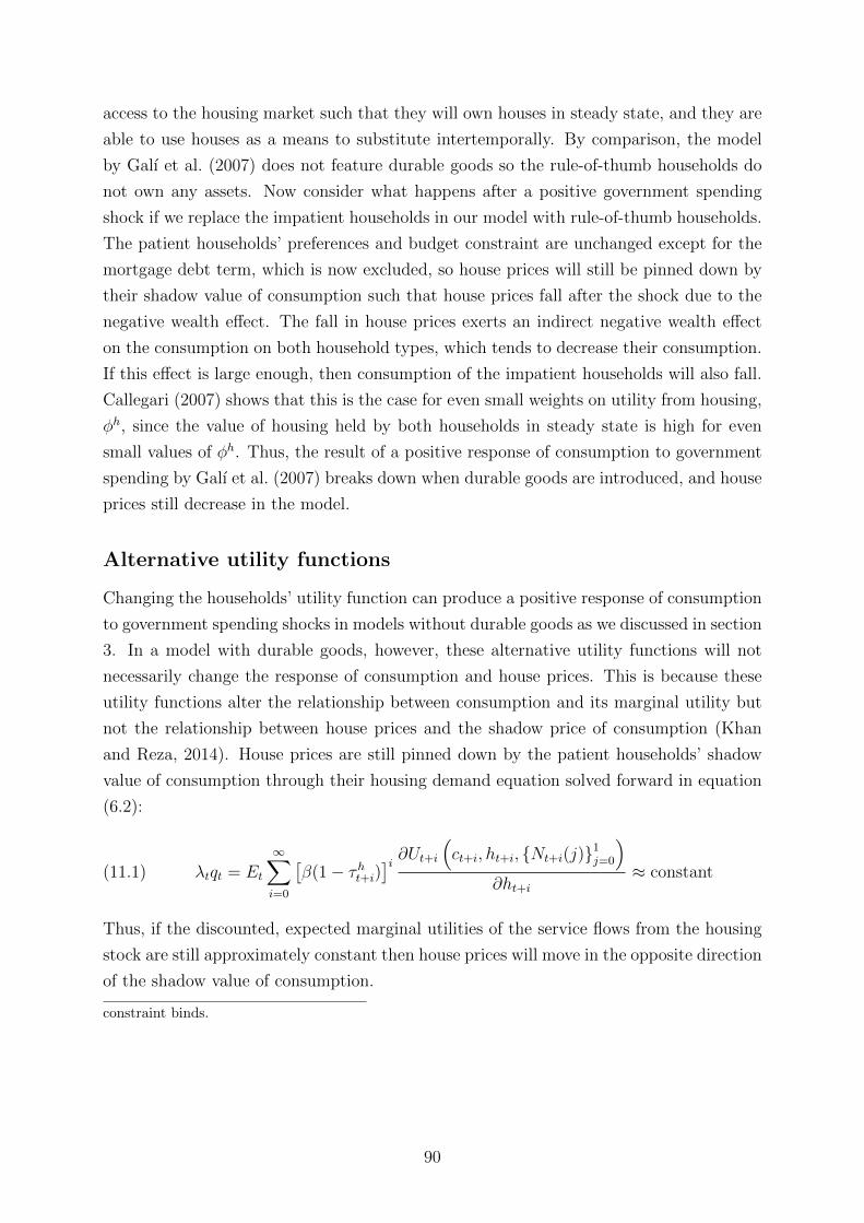
access to the housing market such that they will own houses in steady state, and they are

able to use houses as a means to substitute intertemporally. By comparison, the model

by Galı et al. (2007) does not feature durable goods so the rule-of-thumb households do

not own any assets. Now consider what happens after a positive government spending

shock if we replace the impatient households in our model with rule-of-thumb households.

The patient households’ preferences and budget constraint are unchanged except for the

mortgage debt term, which is now excluded, so house prices will still be pinned down by

their shadow value of consumption such that house prices fall after the shock due to the

negative wealth effect. The fall in house prices exerts an indirect negative wealth effect

on the consumption on both household types, which tends to decrease their consumption.

If this effect is large enough, then consumption of the impatient households will also fall.

Callegari (2007) shows that this is the case for even small weights on utility from housing,

φh, since the value of housing held by both households in steady state is high for even

small values of φh. Thus, the result of a positive response of consumption to government

spending by Galı et al. (2007) breaks down when durable goods are introduced, and house

prices still decrease in the model.

Alternative utility functions

Changing the households’ utility function can produce a positive response of consumption

to government spending shocks in models without durable goods as we discussed in section

3. In a model with durable goods, however, these alternative utility functions will not

necessarily change the response of consumption and house prices. This is because these

utility functions alter the relationship between consumption and its marginal utility but

not the relationship between house prices and the shadow price of consumption (Khan

and Reza, 2014). House prices are still pinned down by the patient households’ shadow

value of consumption through their housing demand equation solved forward in equation

(6.2):

λtqt = Et

∞∑i=0

[β(1− τht+i)

]i ∂Ut+i (ct+i, ht+i, {Nt+i(j)}1j=0

)∂ht+i

≈ constant(11.1)

Thus, if the discounted, expected marginal utilities of the service flows from the housing

stock are still approximately constant then house prices will move in the opposite direction

of the shadow value of consumption.

constraint binds.

90

Edgeworth complementarity between consumption and government spending

First, consider the case where government spending enters a utility function that is sepa-

rable in consumption, housing and labor similar to the utility function analyzed by Khan

and Reza (2014) (ignoring habit formation and labor preferences):

U(ct, ht, gt) = ln(ct + acgt) + φh ln(ht + ahgt)(11.2)

The first-order conditions with respect to consumption and housing for the patient house-

holds are:

(1 + τ ct )λt = ξβt1

ct + acgt(11.3)

λtqt = ξβt ξht

φh

ht + ahgt+ βEt

[(1− τht+1)qt+1λt+1

](11.4)

When ac < 0 and ah < 0, the marginal utilities of consumption and housing are increasing

in government spending such that they are both Edgeworth complements in utility with

government spending. Solving the first-order condition with respect to housing forward

yields:

λtqt = Et

∞∑i=0

[β(1− τht+i)

]ξβt+iξ

ht+i ·

φh

ht+i + ahgt+i(11.5)

If ah = 0 and ac < 0 then the housing demand equation is unchanged and house prices are

pinned down by the shadow value of consumption. If it is also the case that ah < 0 then

changes in government spending can also affect the shadow value of housing because higher

government spending will shift the housing demand curve outwards. Hence, Edgeworth

complementarity can in principle break the constant property of the shadow value of

housing in equation (11.1) but house prices will still move in the opposite direction of the

shadow value of consumption holding all other terms equal.

While higher government spending has a tendency to increase the shadow value of

consumption, it does not necessarily increase since this also depends on the response of

consumption, which will tend to rise due to Edgeworth complementarity between govern-

ment spending and consumption and thereby make the shadow value of consumption fall.

Thus, because Edgeworth complementarity breaks up the relationship between consump-

tion and its shadow value but not the relationship between house prices and the shadow

value of consumption, it will not guarantee an increase in house prices following a positive

government spending shock. Consumption, however, can increase since ac < 0. Khan and

Reza (2014) show that this type of preferences can induce an increase in consumption

of the patient households after a positive government spending shock but still cannot

break the constant property of the shadow value housing so house prices will fall as the

91

marginal utility of consumption increases. The impatient households’ consumption falls

as their collateral constraint is tightened by the drop in house prices.

Monacelli and Perotti (2008) type preferences

Khan and Reza (2014) also analyze the case of non-separable preferences with no wealth

effects on labor supply studied by Monacelli and Perotti (2008). This has two important

implications in a model with durable goods. First, the wealth effects on labor supply

are not eliminated when durable goods are included in the non-separable utility function.

To see this consider the utility function used by Bermperoglou (2015), wherein consump-

tion and housing enter the utility function as an aggregate good Xt defined by the CES

aggregator:

U(ct, ht, Lt) =(Xt − ΦLϕt )1−σ − 1

1− σwhere Xt =

[(1− αh)

1η c

η−1η

t + α1η

h hη−1η

t

] ηη−1

(11.6)

The first-order condition with respect to labor supply yields the following expression for

the labor supply curve:

Lt =

wt(1− τwt )(

(1−αh)Xtct

) 1η

(1 + τ ct )ϕΦ

1

ϕ−1

(11.7)

If houses do not yield utility then αh = 0 and neither consumption nor the housing stock

enter the labor supply curve. Instead, the labor supply curve simply reduces to a function

of real wages and the tax rates as in the model by Monacelli and Perotti (2008):

Lt =

[wt(1− τwt )

(1 + τ ct )ϕΦ

] 1ϕ−1

(11.8)

In the case that αh ∈]0; 1[, then changes in either consumption or the housing stock will

shift the labor supply curve. This shift can offset the large real wage increase, which drove

the positive response of consumption in Monacelli and Perotti’s (2008) model.

Second, the marginal utility of consumption is increasing in labor supply for the utility

function in equation (11.6). This implies that as labor supply increases to accommodate

the higher demand from government spending, the marginal utility of consumption will

tend to increase, which exacerbates the negative wealth effect from the government spend-

ing shock. Hence, house prices must decline more since they are still pinned down by the

patient households’ marginal utility of consumption. This amplifies the decrease in ag-

gregate consumption even further through the collateral constraint channel. Thus, the

non-separable utility function actually amplifies the decrease in both consumption and

house prices in constrast to the separable utility function as shown by Bermperoglou

92

(2015).

Deep habit formation

Finally, Khan and Reza (2014) analyze the deep habit formation preferences introduced

by Ravn et al. (2006):

U (xt, ht, Lt) =

[xφxt h

φht (1− Lt)1−φx−φh

]1−σ− 1

1− σ(11.9)

where xt is a composite of habit-adjusted consumption goods i ∈ [0; 1] similar to the

formulation of deep habits in section 3.

The housing demand curve for the patient households in equation (11.1) still pins

down house prices so if the shadow price of habit-adjusted consumption xt increases after

a positive government spending shock then house prices must fall. The positive response

consumption in the deep habit formation framework relies on a substitution effect from

leisure to consumption as real wages rise that is strong enough to offset the negative wealth

effect. This strong substitution effect is obtained through the countercyclical desired price

markup. The negative wealth effect, however, still decreases the shadow price of habit-

adjusted consumption so house prices will fall. Thus, consumption can rise in the deep

habit formation framework but house prices will still fall.

Monetary accommodation

We discussed how the response of the central bank has a significant impact on the effect

of government spending in section 9. Extending the model with a Taylor rule that ac-

commodates government spending can yield an increase in both consumption and house

prices following an increase in government spending. Consider the following log-linearized

Taylor rule used by Nakamura and Steinsson (2014):

rt = φRrt−1 + (1− φR) [φππt + φyyt + φggt] + ln εRt(11.10)

The central bank accommodates government spending by lowering the interest rate in

responds to an increase in government spending when φg < 0. We add this rule to the

estimated model and set φg = −0.1 such that an increase in government spending by 1 %

will cause the central bank to gradually lower the interest rate by 0.1 percentage points.

We compare the impulse response function to a 1 % increase in government spending in this

model with the impulse response function in the model without monetary accommodation

in figure 11.1. The response of government spending to output and government debt has

been shut off in both models such that the expected path for government spending is

identical for the two models.

93

Figure 11.1: Monetary accommodation and government spending

0

0

Monetary accommodation Baseline

0 5 10 15 20

-0.1

0

0.1

0.2

0.3

0.4

0.5

Output

0 5 10 15 20

-0.2

-0.1

0

0.1

0.2

0.3

0.4

Investment

0 5 10 15 20

-0.04

-0.03

-0.02

-0.01

0

Real wage

0 5 10 15 20

-0.15

-0.1

-0.05

0

0.05

0.1

0.15

Aggregate consumption

0 5 10 15 20

-0.1

-0.05

0

0.05

0.1

Cons. (patient)

0 5 10 15 20

-0.2

-0.1

0

0.1

0.2

0.3

0.4

Cons. (impatient)

0 5 10 15 20

0

0.05

0.1

0.15

0.2

Inflation

0 5 10 15 20

0

0.05

0.1

0.15

0.2

Nominal interest rate

0 5 10 15 20

-0.06

-0.05

-0.04

-0.03

-0.02

-0.01

0

0.01

Exp. real interest rate

0 5 10 15 20

-0.1

-0.05

0

0.05

0.1

0.15

House price

0 5 10 15 20

-0.5

0

0.5

1

1.5

Mortgage debt

0 5 10 15 20

-0.2

-0.15

-0.1

-0.05

0

0.05

0.1

Housing (patient)

Note: The expected path for government spending is identical in both models (i.e. ρG,y = ρG,b = 0). Thex-axis denotes quarters, while the y-axis denotes percentage deviations from steady state (the y-axismeasures percentage point deviations from steady state for inflation, the nominal interest rate and theexpected real interest rate that are annualized).

When monetary policy accommodates fiscal policy then the expected real interest

rate falls considerably on impact after a positive government spending shock. The large

decrease in the real interest rate causes the households to substitute towards current

consumption, which counteracts the negative wealth effect from the government spend-

ing shock. Hence, consumption crowds in, and the decrease in the patient households’

marginal utility of consumption causes house prices to increase. The consumption re-

sponse of the impatient households is significantly larger than that of the patient house-

holds, while investment also crowds in when monetary policy accommodates fiscal policy.

Thus, output increases much more – 0.41 per cent on impact – and the impact multiplier

is close to 2.1 in comparison to the impact multiplier of just about 1 in the baseline model.

The reason why monetary accommodation results in an increase in both consump-

tion and house prices is because of the decrease in the real interest rate. This forces the

shadow value of consumption to fall through the Euler equation and thereby increasing

consumption and house prices. While the alternative utility functions altered the relation-

94

ship between consumption and its marginal utility, monetary accommodation does not.

Instead, it brings about the decrease in the marginal utility of consumption necessary for

an increase in house price, which the alternative utility functions cannot.

12 Discussion: Occasionally binding collateral con-

straints and the zero lower bound

We assumed that the collateral constraint always binds. This was mostly due to analytical

convenience as solving and estimating a model with occasionally binding constraints is a

not a trivial task. On the other hand, assuming that the collateral constraint always binds

might not be very realistic as housing wealth can deviate considerably and persistently

from its trend as shown in figure 12.1.

Figure 12.1: Housing wealth in the United States, 1952-2015

55 60 65 70 75 80 85 90 95 00 05 10 15

% d

ev.

fro

m t

ren

d

-30

-20

-10

0

10

20

30

40

Note: Housing wealth has been calculated as the sum of households’ and nonprofit organizations’ realestate and nonfinancial noncorporate businesses’ residential real estate. The sources are tables B.101(line 3) and B.104 (line 4) in the Z.1 Financial Accounts of the United States downloaded on 21 June2016 from federalreserve.gov. The housing wealth series has been deflated with the GDP deflator,log-transformed and detrended with a quadratic trend.

If these deviations cause the collateral constraint to become slack, then the dynamics

of the model behave differently and the model’s predictions for the transmission of fiscal

policy shocks will be misleading. Luckily, two recent papers by Guerrieri and Iacoviello

(2016) and Bermperoglou (2015) can guide use towards an idea about how our model

would behave with an occasionally binding collateral constraint.

Guerrieri and Iacoviello (2016) solve and estimate a New Keynesian model similar to

ours with two occasionally binding constraints: a collateral constraint and the zero lower

95

bound on the interest rate. They show that this model implies that there is an important

asymmetric macroeconomic reaction to shocks affecting house prices. As an example,

consider a protracted boom in house prices followed by a bust similar to the recent house

price cycle in the United States from the late 1990s until the Great Recession. When

the collateral constraint binds and house prices rise during the boom period, this fuels

an increase in consumption that is driven by debt. As some point, however, housing

wealth and the borrowing capacity of the impatient households increase so much that the

collateral constraint becomes slack and the increasing house prices no longer contribute

to consumption growth through the collateral constraint. By contrast, as the boom turns

to bust and house prices fall, the collateral constraint eventually becomes binding again,

which causes consumption to fall as the impatient households are forced to deleverage.

However, the collateral constraint does not become slack again as house prices continue

to fall. Thus, the asymmetric macroeconomic reaction to house prices occurs because the

collateral constraint can eventually become slack during booms in house prices, while this

is not the case during busts, where deleveraging pressures will continue as house prices

fall.

The estimation procedure used by Guerrieri and Iacoviello (2016) enables them to infer

when the two constraints bind or not, and they find that the collateral constraint was not

binding from the late-90s until 2007.43 This implies that the increasing house prices

contributed little to consumption growth prior to the Great Recession, while they drove

a considerable part of the decline in consumption during the housing bust. Indeed, the

model attributes about 70 per cent of the consumption decline through 2009 to housing

demand shocks, while these shocks contributed almost nothing to consumption during

the prior house price boom. By comparison, housing demand shocks explain the better

part of the movements in house price throughout the sample period of 1985Q1-2011Q4.

It might seem a bit surprising that housing preference shocks explain such a large share

of the consumption decline during the Great Recession – taken literally this implies that

a sudden and persistent distaste for houses caused the bust in house prices as well as the

large decline in consumption – but this is largely a consequence of the simplistic nature

of the model, which includes few shocks.44

Bermperoglou (2015) is the only author that we know of who has analyzed the non-

linear dynamics caused by an occasionally binding collateral constraint in the transmission

of fiscal policy. The non-fiscal block of his model is identical to ours except that he 1)

excludes capital from the model, 2) includes housing production similar to Iacoviello and

43Although house prices started falling in 2005, the collateral constraint did not immediately becomebinding in 2005 since housing wealth was high at the start of the house price bust. Consequently, thecollateral constraint only starts to bind again in 2007 when housing wealth has declined sufficiently.

44Iacoviello (2015) estimate of model with an always binding collateral constraint that provides anexplanation for the Great Recession, which might seem more plausible. In this model, recessions can becaused by losses suffered by banks, which affect their ability to extend credit to the real sector.

96

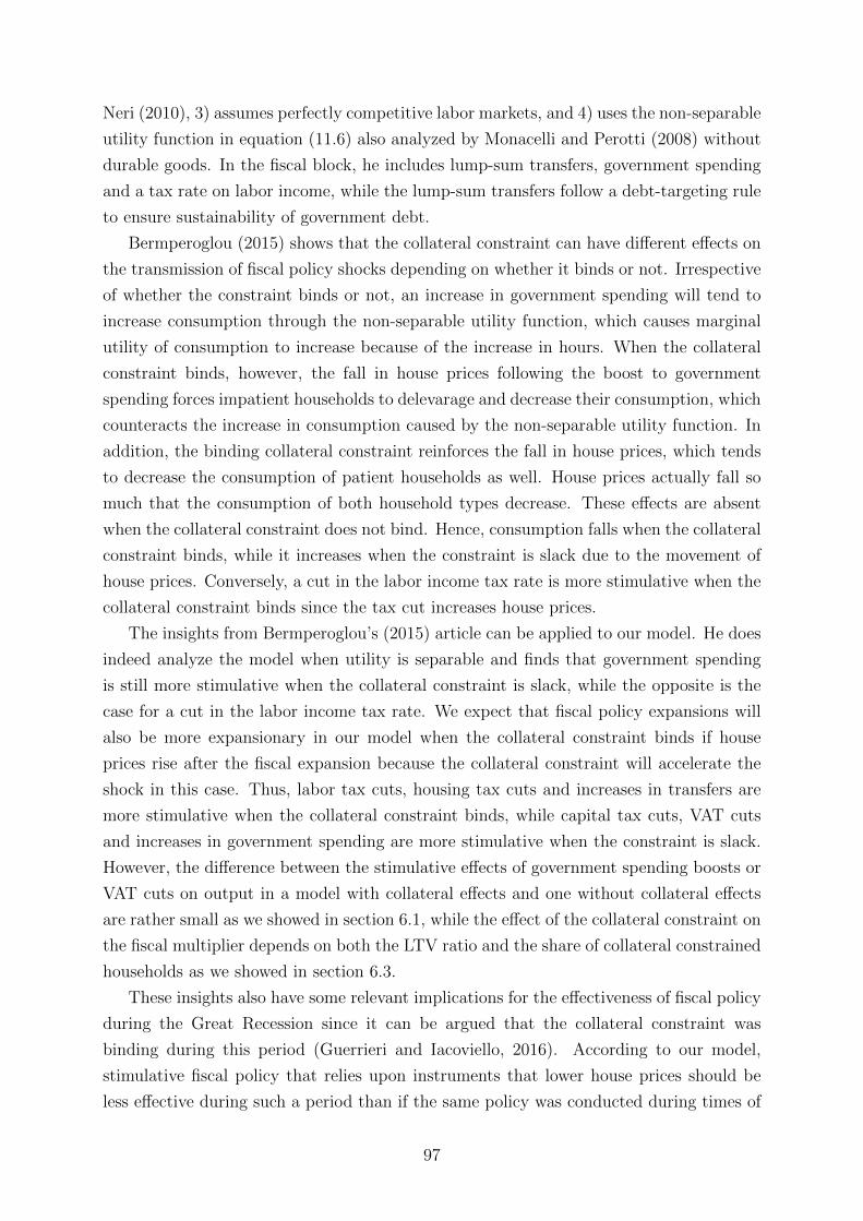
Neri (2010), 3) assumes perfectly competitive labor markets, and 4) uses the non-separable

utility function in equation (11.6) also analyzed by Monacelli and Perotti (2008) without

durable goods. In the fiscal block, he includes lump-sum transfers, government spending

and a tax rate on labor income, while the lump-sum transfers follow a debt-targeting rule

to ensure sustainability of government debt.

Bermperoglou (2015) shows that the collateral constraint can have different effects on

the transmission of fiscal policy shocks depending on whether it binds or not. Irrespective

of whether the constraint binds or not, an increase in government spending will tend to

increase consumption through the non-separable utility function, which causes marginal

utility of consumption to increase because of the increase in hours. When the collateral

constraint binds, however, the fall in house prices following the boost to government

spending forces impatient households to delevarage and decrease their consumption, which

counteracts the increase in consumption caused by the non-separable utility function. In

addition, the binding collateral constraint reinforces the fall in house prices, which tends

to decrease the consumption of patient households as well. House prices actually fall so

much that the consumption of both household types decrease. These effects are absent

when the collateral constraint does not bind. Hence, consumption falls when the collateral

constraint binds, while it increases when the constraint is slack due to the movement of

house prices. Conversely, a cut in the labor income tax rate is more stimulative when the

collateral constraint binds since the tax cut increases house prices.

The insights from Bermperoglou’s (2015) article can be applied to our model. He does

indeed analyze the model when utility is separable and finds that government spending

is still more stimulative when the collateral constraint is slack, while the opposite is the

case for a cut in the labor income tax rate. We expect that fiscal policy expansions will

also be more expansionary in our model when the collateral constraint binds if house

prices rise after the fiscal expansion because the collateral constraint will accelerate the

shock in this case. Thus, labor tax cuts, housing tax cuts and increases in transfers are

more stimulative when the collateral constraint binds, while capital tax cuts, VAT cuts

and increases in government spending are more stimulative when the constraint is slack.

However, the difference between the stimulative effects of government spending boosts or

VAT cuts on output in a model with collateral effects and one without collateral effects

are rather small as we showed in section 6.1, while the effect of the collateral constraint on

the fiscal multiplier depends on both the LTV ratio and the share of collateral constrained

households as we showed in section 6.3.

These insights also have some relevant implications for the effectiveness of fiscal policy

during the Great Recession since it can be argued that the collateral constraint was

binding during this period (Guerrieri and Iacoviello, 2016). According to our model,

stimulative fiscal policy that relies upon instruments that lower house prices should be

less effective during such a period than if the same policy was conducted during times of

97

non-binding constraints. The American Recovery and Reinvestment Act of 2009 – which

was the $787 billion fiscal stimulus package enacted in response to the Great Recession

– consisted of a plethora of instruments: about a half of the package went to temporary

tax cuts and increased transfers, while the remaining portion of the package consisted of

mostly government spending programs including infrastructure, research, education and

health care programs (Cogan et al., 2010). Some of these actions will cause house prices

to increase, while others will cause them to fall.

We should also remember that monetary policy hit the zero lower bound by the end

of 2008 and remained there until the end of 2015. Hence, the American economy was in

a regime with both a binding collateral constraint and monetary policy up against the

zero lower bound during the Great Recession (Guerrieri and Iacoviello, 2016). As shown

in the previous section, expansionary government spending can become very effective in

this type of regime since the accommodative monetary policy causes the real interest rate

to decline, which boosts consumption and house prices.45 The large stimulative effects

of government spending at the zero lower bound is a normal feature of New Keynesian

models as also analyzed by Christiano et al. (2011) and Woodford (2011) among others

but our model includes an additional channel that stimulates consumption: the increase

in house prices loosen the collateral constraint for the impatient households, which tends

to increase consumption further. Whether the other fiscal instruments are also more

effective at the zero lower bound will not only depend on how house prices behave. It will

also depend on how goods prices are affected since fiscal instruments with deflationary

effects might actually worsen a recession when the nominal interest rate is trapped at

the zero lower bound because this causes the real interest rate to increase. Thus, cuts in

either capital or labor income taxes can be contractionary at the zero lower bound since

they have deflationary effects on the economy (Eggertsson, 2011).46 By contrast, higher

transfers or cuts in the VAT rate and the housing tax rate have inflationary effects, which

will decrease the real interest rate at the zero lower bound and further stimulate the fiscal

expansion. We should, however, take into account that these effects might be different if

the economy is trapped in a expectations-driven liquidity trap instead of a fundamental

liquidity trap as we discussed in section 3.

45The regime we analyzed in the previous section is not the same as a regime with a binding zero lowerbound. We should, however, still expect that the real interest rate will decrease when the zero lowerbound binds, which stimulates consumption.

46As we discussed in section 6.1, the model actually implies that inflation increases after a cut in laborincome taxes. This was because capital tax rates will increase following the tax cut, which might be anunrealistic assumption if the labor income tax cut is part of a larger stimulus package.

98

13 Discussion: Comparison with Andres et al.’s (2015)

model

Our analysis is closely related to the work of Andres et al. (2015). They also analyze

government spending shocks in a model with collateral constraints and frictions in the

labor market that create unemployment. Their model differs, however, from ours in

two important ways. First, our model includes a staggered wage setting mechanism and

unemployment results from unions’ market power in the labor market. They include

search and match frictions in the labor market in their model such that trade in the labor

market is subject to transaction costs. The labor inputs from the households are perfect

complements in their model and the common wage is set through a Nash bargaining

process between firms and a union that maximizes a weighted average of the households’

surplus from working. Second, we include distortionary taxation in our model, while

government spending is financed by bond issuance and lump-sum taxes in their model.47

Andres et al.’s (2015) model is able to produce a crowding-in effect in impatient

households’ consumption after a government spending shock, while consumption of both

household types fall after a positive government spending shock in the model we have

analyzed. Hence, as long as the share of impatient households in their model is sufficiently

large then aggregate consumption will also increase. Andres et al. (2015) find that the

share of impatient households actually does not need to be large – only slightly above

20 per cent – to produce an increase in aggregate consumption as long as the LTV ratio

is high (they set the LTV ratio at 0.985). Similar to our model, both house prices and

consumption of the patient households decrease after the government spending shock. In

contrast to our model, however, mortgage debt increases on impact in their model, which

is only possible if the impatient households increase their housing stock sufficiently when

house prices fall and the expected real interest rate increases following the shock.

We suspect that the difference in the impatient households’ consumption response in

the two models is mainly because of the two different labor market frameworks since con-

sumption still decreases in our model if higher government spending is financed through

lower lump-sum transfers instead of higher distortionary tax rates. Andres et al. (2015)

also stress the importance of an increase in labor income for producing the increase in

impatient households’ consumption since their consumption is highly dependent on la-

bor income when the LTV ratio is high as we discussed in section 6.3. Thus, if labor

income increases following the boost to government spending then impatient households’

consumption also increase. This mechanism is also present in our model. Actually, if we

decrease the degree of wage stickiness by lowering the value of θw sufficiently such that

47Andres et al. (2016) have later augmented their model with distortionary taxes on labor income,consumption and capital income as well social security contributions payed by firms. The taxes react togovernment debt to ensure sustainability of the government debt.

99

nominal wages react more to the countercyclical wage markup, then the model is able to

produce an increase in impatient households’ consumption after a shock to government

spending. This is shown in figure 13.1 below, where we have set θw = 0.2 and compare

the impulse response functions for consumption and the labor market variables with the

impulse response functions in a model, wherein the parameters are fixed at their pos-

terior means. We also shut down the response of government spending to output and

government debt such that the path of government spending is the same in the two cases.

Figure 13.1: Nominal wage rigidities and government spending shocks

0

0Low wage stickiness, θw

=0.2 Baseline, θw

= 0.904

0 5 10 15 20

-0.14

-0.12

-0.1

-0.08

-0.06

-0.04

-0.02

0

Aggregate consumption

0 5 10 15 20

-0.15

-0.1

-0.05

0

Consumption (patient)

0 5 10 15 20

-0.2

-0.15

-0.1

-0.05

0

0.05

0.1

Consumption (impatient)

0 5 10 15 20

-0.1

-0.05

0

0.05

0.1

0.15

0.2

0.25

Real wage

0 5 10 15 20

-0.2

-0.15

-0.1

-0.05

0

0.05

Unemployment

0 5 10 15 20

-0.05

0

0.05

0.1

0.15

0.2

Employment

Note: The blue solid lines are the impulse responses for the model with θw = 0.2 and ρg,b = ρg,y = 0,while the dashed magenta lines are the impulse responses for the model with parameters fixed at theposterior mean estimates expect for the response of government spending to output and governmentdebt, which is shut down (i.e. θw = 0.904, ρg,b = 0 and ρg,y = 0). x-axis denotes quarters, while y-axisdenotes percentage deviations from steady state (the y-axis measures percentage point deviations fromsteady state for the unemployment rate).

The low degree of wage rigidity implies that real wages increase after the boost to

government spending. Combined with higher employment, this increases labor income

and results in an increase in the impatient households’ consumption.48 This is not suffi-

cient, however, to induce crowding-in effects in aggregate consumption. Similar to Andres

et al. (2015), we also see some degree of decoupling between aggregate consumption and

employment as well as unemployment when wages are more flexible: the responses of both

unemployment and employment is more muted when real wages increase, while aggregate

consumption responds more on impact.

48Note that the labor income tax rate gradually increases following the shock, which will tend todecrease labor income after taxes.

100

Two aspects are important for the positive response of the impatient households’

consumption in figure 13.1. First, the response relies on a high LTV ratio. If the LTV

ratio is too low then a smaller share of the impatient households’ housing stock is financed

by debt such that the lower house prices will tend to decrease their consumption and

thereby counteract the effect on consumption from higher labor income. This is similar

to the results of Andres et al. (2015) who find that aggregate consumption will only

increase if the LTV ratio is high.49 Second, the relative rigidity between wages and prices

is important for the increase in real wages as highlighted by Galı (2013): prices need to be

sufficiently rigid in comparison to wages to generate the real wage increase. This can be

seen be noting that the price and wage rigidities drive a time-varying markup (or wedge)

between the marginal product of labor and the real wage:

wt − pt + µpt = mpnt(13.1)

where µpt is the log of the markup and mpnt is the log of the marginal product of labor.

When an increase in government spending boosts aggregate demand and employment,

the marginal product of labor falls, which tends to reduce the real wage. The markup,

however, is countercyclical and will fall. If this fall in the markup more than offsets the

fall in the marginal product of labor then the real wage will increase. Stickier prices will

induce a larger decrease in the markup making a real wage increase more likely. If wages

on the other hand become stickier then the rise in the marginal costs of firms becomes

smaller, which tends to lessen the decrease in the markup. This makes it less likely that

the markup will offset the fall in the marginal product of labor and thereby increase the

real wage. Thus, prices need to be sufficiently sticky relative to wages for the real wage

and also the impatient households’ consumption to increase in our model following an

increase in government spending.

The search and match frictions in Andres et al.’s (2015) model have a further effect

on the response of consumption that is not present in our model. When the consumption

of the impatient households increases following the boost to government spending, they

push for higher wages, while the opposite is true for the patient households’ consumption,

which decreases. This effect on the wage bargaining process is stronger when the LTV

ratio is high since this increases impatient households’ consumption but it is also stronger

when the share of impatient households is large since the impatient households’ surplus

from working has a higher weight in the union’s maximization problem. Hence, the LTV

ratio and the share of impatient households tend to reinforce each other’s positive effect

on real wages. These wage bargaining effects on wages are not present in the labor market

framework in our model.

49They analyze government spending multipliers for two different LTV ratios: a low value of 0.7 anda high value 0.985. Only the model with a high LTV ratio is able to produce a crowding-in effect inaggregate consumption.

101

14 Conclusion

This thesis looked at how collateral constraints tied to housing values affects the trans-

mission of fiscal policy. We constructed a DSGE model containing the housing market

in the model by Iacoviello and Neri (2010) as well as a rich fiscal policy block similar to

the formulation by Zubairy (2014) and an reformulation of a standard staggered wage

setting mechanism by Galı (2011a), which introduces a measure of unemployment into

the model. The model was subsequently estimated on quarterly U.S. data covering the

period of 1985Q1-2007Q4.

We find that the collateral constraint can either increase or decrease the fiscal mul-

tiplier depending on the direction of house prices following a shock to fiscal policy. The

mechanism is the same as in the model by Iacoviello (2005): if house prices increase,

then the consumption of collateral constrained households increases as their collateral

constraint is relaxed. Vice versa, their consumption will fall if house prices fall. Hence, a

fiscal expansion using a boost in government spending or cuts in capital and consumption

tax rates – all which lower house prices – will be decelerated by the collateral constraint,

while a fiscal expansion using increased lump-sum transfers to households or cuts in labor

or housing tax rates – all which increase house prices – will be accelerated. These effects

are more pronounced when households can borrow against a larger share of their housing

value. We find, however, that the effect of the collateral constraint on the multiplier is

rather small for the government spending and the VAT rate shocks in our estimated model.

The effect of the collateral constraint on the present value fiscal multipliers for these two

fiscal instruments is also small, and the effect on short-run and long-run multipliers differs.

We calculated posterior mean fiscal multipliers based on the posterior distribution of

the parameters of the model. The impact multiplier for government spending is 0.94, while

the impact multipliers for cuts in consumption, capital, labor and housing tax rates are

0.62, 0.25, 0.25 and 0.21 respectively when total tax revenue increases by 1 % on impact

after a shock. The lump-sum transfers multiplier is 0.29 on impact. While government

spending has the largest effect on impact, the effects of the other fiscal instruments take

some time to build. For example, the present value multiplier for a capital tax cut is 3.00

at the 20th quarter horizon, while the present value multiplier for a labor tax cut is 0.37

and -0.39 at the 4th and 20th quarter horizon respectively.

We did not perform any investigations into the econometric aspects of our model. A

few of the posterior estimates of the parameters that we obtained were a little suspect:

the central bank smooths interest rates a lot, the degree of wage rigidity is relatively high,

the wage markup is very persistent and the wage indexation parameter is a lot higher

than what is usually found in the literature. It could be interesting to explore why these

estimates differ from what is usually found in the literature. In addition, we performed

no robustness checks such as estimating the model on different sample periods, using

102

alternative data for the observables or evaluating the fit of the model. Lastly, the LTV

ratio has a noticeable effect on fiscal multipliers but we only calibrated this parameter,

which could be interesting to estimate more formally.

There is ample room for theoretical extensions of our analysis. First, the model cannot

produce an increase in both house prices and consumption following a boost to government

spending, which is something that some authors have found in SVAR analyses of fiscal

policy. Changing the households’ utility function to other preference structures usually

used as explanations for the comovement between consumption and government spending

in models without durable goods does not change this. Monetary accommodation, how-

ever, does. Hence, it would be interesting to further explore how a model with a housing

market can modified such that house prices and consumption rise following an increase in

government spending. Second, we argued that the collateral constraint is only occasionally

binding in reality, while we assumed during our analysis that it is always binding. Further

exploring how the transmission of fiscal policy is affected by an occasionally binding col-

lateral constraint would be interesting. Third, we used a rather simplistic reformulation

of the standard New Keynesian labor market to include a measure of unemployment in

our model. The labor market structure not only affects the dynamics of the model but

unemployment is also an important economic phenomenon so analyzing the model with

alternative labor market structures would be relevant.

Finally, our results indicate that fiscal multipliers are sensitive to not only monetary

policy but also to how the government finances a fiscal expansion. In the words of Leeper

(2016), these are just two of the reasons for why fiscal policy analysis is “darned hard”. In-

side lags in fiscal actions, expectational effects, the plethora of different fiscal instruments

in the real world, supranational institutions imposing constraints on policy, political as-

pects and automatic stabilizer built into tax codes are some other reasons for why fiscal

policy analysis is difficult. Luckily, the academic interest in fiscal policy has been renewed

in recent years and economists have begun integrating some of these aspects into models,

which will hopefully make fiscal policy analysis more relevant for policy makers.

103

References

Abraham, K. G., Spletzer, J. R., and Stewart, J. C. (1999). Why Do Different Wage

Series Tell Different Stories? American Economic Review, 89(2):34–39.

Afonso, A. and Sousa, R. M. (2012). The macroeconomic effects of fiscal policy. Applied

Economics, 44(34):4439–4454.

Alpanda, S. and Zubairy, S. (2016). Housing and Tax Policy. Journal of Money, Credit

and Banking, 48(2-3):485–512.

Andre, C. (2010). A Bird’s Eye View of OECD Housing Markets. OECD Economics

Department Working Papers No. 746.

Andres, J., E. Bosca, J., and Ferri, J. (2015). Household Debt and Fiscal Multipliers.

Economica, 82:1048–1081.

Andres, J., E. Bosca, J., and Ferri, J. (2016). Instruments, rules, and household debt: the

effects of fiscal policy. Oxford Economic Papers, 68(2):419–443.

Auerbach, A. J. and Gorodnichenko, Y. (2012). Measuring the Output Responses to

Fiscal Policy. American Economic Journal: Economic Policy, 4(2):1–27.

Barsky, R. B., House, C. L., and Kimball, M. S. (2007). Sticky-Price Models and Durable

Goods. American Economic Review, 97(3):984–998.

Baxter, M. and King, R. G. (1993). Fiscal Policy in General Equilibrium. American

Economic Review, 83(3):315–334.

Berger, D. and Vavra, J. (2012). Measuring How Fiscal Shocks Affect Durable Spending

in Recessions and Expansions. American Economic Review, 104(5):112–115.

Bermperoglou, D. (2015). Three Essays on Fiscal Policy. PhD thesis, Universitat

Autonoma de Barcelona. Chapter: ”Non-linear effects of fiscal policy: the role of

housing wealth and collateral constraints”.

Bernanke, B. S., Gertler, M., and Gilchrist, S. (1999). The financial accelerator in a

quantitative business cycle framework. In Taylor, J. B. and Woodford, M., editors,

Handbook of Macroeconomics, volume 1 of Handbook of Macroeconomics, chapter 21,

pages 1341–1393. Elsevier.

Bilbiie, F. O. (2009). Nonseparable Preferences, Fiscal Policy Puzzles, and Inferior Goods.

Journal of Money, Credit and Banking, 41(2-3):443–450.

104

Blanchard, O. and Perotti, R. (2002). An Empirical Characterization of the Dynamic

Effects of Changes in Government Spending and Taxes on Output. Quarterly Journal

of Economics, 117(3):1329–1368.

Bouakez, H. and Rebei, N. (2007). Why Does Private Consumption Rise After a Govern-

ment Spending Shock? Canadian Journal of Economics, 40(3):954–979.

Burnside, C., Eichenbaum, M., and Fisher, J. (2004). Fiscal Shocks and Their Conse-

quences. Journal of Economic Theory, 115(1):89–117.

Callegari, G. (2007). Fiscal Policy and Consumption. PhD thesis, European University

Institute. Chapter: ”Government Expenditure, Durable Goods and Rule-of-Thumb

Behavior”.

Calvo, G. A. (1983). Staggered prices in a utility-maximizing framework. Journal of

Monetary Economics, 12(13):383–398.

Cavallo, M. (2005). Government Employment and the Dynamic Effects of Fiscal Policy

Shocks. Working Paper Series 2005-16. Federal Reserve Bank of San Francisco.

Chari, V., Kehoe, P., and McGrattan, E. R. (2009). New Keynesian Models: Not Yet

Useful for Policy Analysis. American Economic Journal: Macroeconomics, 1(1):242–

266.

Chib, S. and Greenberg, E. (1995). Understanding the Metropolis-Hastings Algorithm.

The American Statistician, 49(4):327–335.

Christiano, L., Eichenbaum, M., and Rebelo, S. (2011). When Is the Government Spending

Multiplier Large? Journal of Political Economy, 119(1):78–121.

Christiano, L., Rostagno, M., and Motto, R. (2014). Risk Shocks. American Economic

Review, 104(1):27–65.

Christiano, L. J. (2002). Solving Dynamic Equilibrium Models by a Method of Undeter-

mined Coefficients. Computational Economics, 20(1):21–55.

Christiano, L. J. (2012). Comment on ”Unemployment in an Estimated New Keynesian

Model”. In Acemoglu, D. and Woodford, M., editors, NBER Macroeconomics Annual

2011, Volume 26, pages 361–380. University of Chicago Press, Chicago, Illinois.

Christiano, L. J., Eichenbaum, M., and Evans, C. L. (2005). Nominal Rigidities and the

Dynamic Effects of a Shock to Monetary Policy. Journal of Political Economy, 113(1):1

– 45.

105

Cogan, J. F., Cwik, T., Taylor, J. B., and Wieland, V. (2010). New Keynesian versus old

Keynesian government spending multipliers. Journal of Economic Dynamics & Control,

34(3):281–295.

Davig, T. and Leeper, E. M. (2011). Monetary-fiscal policy interactions and fiscal stimulus.

European Economic Review, 55(2):211–222.

Eggertsson, G. B. (2011). What Fiscal Policy is Effective at Zero Interest Rates? In

Acemoglu, D. and Woodford, M., editors, NBER Macroeconomics Annual 2010, pages

59–112. University of Chicago Press, Chicago, Illinois.

Erceg, C. J. and Linde, J. (2014). Is There a Fiscal Free Lunch in a Liquidity Trap?

Journal of the European Economic Association, 12(1):73–107.

Fatas, A. and Mihov, I. (2001). The Effects of Fiscal Policy on Consumption and Em-

ployment: Theory and Evidence. Unpublished manuscript, April.

Fazzari, S. M., Morley, J., and Panovska, I. (2015). State-dependent effects of fiscal policy.

Studies in Nonlinear Dynamics & Econometrics, 19(3):285–315.

Fernandez-Villaverde, J. (2010). The econometrics of DSGE models. SERIEs, 1(1):3–49.

Fernandez-Villaverde, J., Rubio-Ramırez, J. F., and Schorfheide, F. (forthcoming). Solu-

tion and Estimation Methods for DSGE Models. In Taylor, J. B. and Uhlig, H., editors,

Handbook of Macroeconomics, Volume 2. Elsevier Science, Amsterdam.

Fisher, J. D. and Peters, R. (2010). Using Stock Returns to Identify Government Spending

Shocks. The Economic Journal, 120(544):414–436.

Galı, J. (2009). Monetary Policy, Inflation, and the Business Cycle: An Introduction to

the New Keynesian Framework. Princeton University Press, 1. edition.

Galı, J. (2011a). The Return of the Wage Phillips Curve. Journal of the European

Economic Association, 9(3):436–461.

Galı, J. (2011b). Unemployment Fluctuations and Stabilization Policies: A New Keyne-

sian Perspective. The MIT Press, Cambridge, Massachusetts, 1. edition.

Galı, J. (2013). Notes for a New Guide to Keynes (I): Wages, Aggregate Demand, and

Employment. Journal of the European Economic Association, 11(5):973–1003.

Galı, J., Lopez-Salido, J. D., and Valles, J. (2007). Understanding the Effects of Gov-

ernment Spending on Consumption. Journal of the European Economic Association,

5(1):227–270.

106

Galı, J., Smets, F., and Wouters, R. (2012). Unemployment in an Estimated New Key-

nesian Model. In Acemoglu, D. and Woodford, M., editors, NBER Macroeconomics

Annual 2011, Volume 26, pages 329–360. University of Chicago Press, Chicago, Illinois.

Gechert, S. (2015). What fiscal policy is most effective? A meta-regression analysis.

Oxford Economic Papers, 67(3):553–580.

Gerali, A., Neri, S., Sessa, L., and Signoretti, F. M. (2010). Credit and Banking in a DSGE

Model of the Euro Area. Journal of Money, Credit and Banking, 42(s1):107–141.

Guerrieri, L. and Iacoviello, M. (2016). Collateral Constraints and Macroeconomic Asym-

metries. Unpublished manuscript, May.

Hamilton, J. D. (1994). Time Series Analysis. Princeton University Press, Princeton,

New Jersey.

Harris, B. H. and Moore, B. D. (2013). Residential Property Taxes in the United States.

Urban-Brookings Tax Policy Center, Washington D.C.

Herbst, E. P. and Schorfheide, F. (2016). Bayesian Estimation of DSGE Models. The

Econometric and Tinbergen Institutes Lectures. Princeton University Press, Princeton,

New Jersey.

Iacoviello, M. (2005). House Prices, Borrowing Constraints, and Monetary Policy in the

Business Cycle. American Economic Review, 95(3):739–764.

Iacoviello, M. (2012). Housing Wealth and Consumption. In Smith, S. J., editor, Interna-

tional Encyclopedia of Housing and Home, pages 673–678. Elsevier Science, Amsterdam,

The Netherlands.

Iacoviello, M. (2015). Financial Business Cycles. Review of Economic Dynamics,

18(1):140–163.

Iacoviello, M. and Neri, S. (2010). Housing Market Spillovers: Evidence from an Estimated

DSGE Model. American Economic Journal: Macroeconomics, 2(2):125–64.

Ingholt, M. M. (2015). Introducing a Housing Collateral Constraint and Union Unem-

ployment into an Estimated DSGE Model. Master’s thesis, University of Copenhagen.

Jacob, P. (2015). Deep Habits, Price Rigidities, and the Consumption Response to Gov-

ernment Spending. Journal of Money, Credit and Banking, 47(2-3):481–509.

Jermann, U. and Quadrini, V. (2012). Macroeconomic Effects of Financial Shocks. Amer-

ican Economic Review, 102(1):238–271.

107

Jones, J. B. (2002). Has fiscal policy helped stabilize the postwar U.S. economy? Journal

of Monetary Economics, 49(4):709–746.

Justiniano, A., Primiceri, G. E., and Tambalotti, A. (2013). Is There a Trade-Off between

Inflation and Output Stabilization? American Economic Journal: Macroeconomics,

5(2):1–31.

Khan, H. and Reza, A. (2014). House Prices and Government Spending Shocks. Unpub-

lished manuscript, August.

Kiyotaki, N. and Moore, J. (1997). Credit Cycles. Journal of Political Economy,

105(2):211–48.

Leeper, E. M. (1991). Equilibria under ’active’ and ’passive’ monetary and fiscal policies.

Journal of Monetary Economics, 27(1):129–147.

Leeper, E. M. (2016). Fiscal Analysis is Darned Hard. Unpublished manuscript, January.

Leeper, E. M., Plante, M., and Traum, N. (2010). Dynamics of fiscal financing in the

United States. Journal of Econometrics, 156(2):304–321.

Leeper, E. M., Richter, A. W., and Walker, T. B. (2012). Quantitative Effects of Fiscal

Foresight. American Economic Journal: Economic Policy, 4(2):115–144.

Leeper, E. M., Traum, N., and Walker, T. B. (2015). Clearing Up the Fiscal Multiplier

Morass. Unpublished manuscript, July.

Leeper, E. M., Walker, T. B., and Yang, S.-C. S. (2013). Fiscal Foresight and Information

Flows. Econometrica, 81(3):1115–45.

Linnemann, L. (2006). The Effect of Government Spending on Private Consumption: A

Puzzle? Journal of Money, Credit and Banking, 38(7):1715–1736.

Linnemann, L. (2011). Nonseparable Preferences, Frisch Labor Supply, and the Con-

sumption Multiplier of Government Spending: One Solution to a Fiscal Policy Puzzle.

Journal of Money, Credit and Banking, 43(1):221–251.

Linnemann, L. and Schabert, A. (2004). Can fiscal spending stimulate private consump-

tion? Economic Letters, 82(2):173–179.

Mertens, K. and Ravn, M. O. (2010). Measuring the Impact of Fiscal Policy in the Face of

Anticipation: A Structural VAR Approach. The Economic Journal, 120(544):393–413.

Mertens, K. and Ravn, M. O. (2012). Empirical Evidence on The Aggregate Effects of

Anticipated and Unanticipated U.S. Tax Policy Shocks . American Economic Journal:

Economic Policy, 4(2):145–181.

108

Mertens, K. and Ravn, M. O. (2013). The Dynamic Effects of Personal and Cor-

porate Income Tax Changes in the United States. American Economic Review,

103(4):1212aAS1247.

Mertens, K. and Ravn, M. O. (2014a). A reconciliation of SVAR and narrative estimates

of tax multipliers. Journal of Monetary Economics, 68, Supplement:S1–S19.

Mertens, K. and Ravn, M. O. (2014b). Fiscal Policy in an Expectations-Driven Liquidity

Trap. Review of Economic Studies, 81(4):1637–1667.

Monacelli, T. and Perotti, R. (2008). Fiscal Policy, Wealth Effects, and Markups. NBER

Working Papers 14584, National Bureau of Economic Research.

Mountford, A. and Uhlig, H. (2009). What are the Effects of Fiscal Policy Shocks? Journal

of Applied Econometrics, 24(6):960–92.

Nakamura, E. and Steinsson, J. (2014). Fiscal Stimulus in a Monetary Union: Evidence

from US Regions. American Economic Review, 104(3):753–792.

Owyang, M. T., Ramey, V. A., and Zubairy, S. (2013). Are Government Spending Mul-

tipliers Greater during Periods of Slack? Evidence from Twentieth-Century Historical

Data. American Economic Review: Papers & Proceedings, 103(3):129–134.

Pedersen, J. and Ravn, S. H. (2013). What Drives the Business Cycle in a Small Open

Economy? Evidence from an Estimated DSGE Model of the Danish Economy. Working

Paper 88, Danmarks Nationalbank.

Perotti, R. (2005). Estimating the effects of fiscal policy in OECD countries. Federal

Reserve Bank of San Francisco: Proceedings.

Pinter, G. (2014). Land-Price Dynamics and Macroeconomic Fluctuations (Liu et al,

Econometrica, 2013): A Comment. Unpublished manuscript, March.

Ramey, V. A. (2011a). Can Government Purchases Stimulate the Economy? Journal of

Economic Literature, 49(3):673–85.

Ramey, V. A. (2011b). Identifying Government Spending Shocks: It’s all in the Timing.

Quarterly Journal of Economics, 126(1):1–50.

Ramey, V. A. (2016). Macroeconomic Shocks and Their Propagation. NBER Working

Papers 21978, National Bureau of Economic Research.

Ramey, V. A. and Shapiro, M. D. (1998). What are the Effects of Fiscal Policy Shocks?

Carnegie-Rochester Conference Series on Public Policy, 48:145–94.

109

Rappaport, J. (2007). A Guide to Aggregate House Price Measures. Federal Reserve Bank

of Kansas City Economic Review, 92(2):41–71.

Ravn, M., Schmitt-Grohe, S., and Uribe, M. (2006). Deep Habits. Review of Economic

Studies, 73(1):195–218.

Romer, C. D. and Romer, D. H. (2010). The Macroeconomic Effects of Tax Changes:

Estimates Based on a New Measure of Fiscal Shocks. American Economic Review,

100(3):763–801.

Schmitt-Grohe, S. and Uribe, M. (2012). What’s News in Business Cycles. Econometrica,

80(6):2733–2764.

Smets, F. and Wouters, R. (2007). Shocks and Frictions in US Business Cycles: A Bayesian

DSGE Approach. American Economic Review, 97(3):586–606.

Stock, J. H. and Watson, M. W. (2003). Has the Business Cycle Changed and Why? In

Gertler, M. and Rogoff, K., editors, NBER Macroeconomics Annual 2002, Volume 17,

pages 159–230. University of Chicago Press, Chicago, Illinois.

Traum, N. and Yang, S.-C. S. (2015). When Does Government Debt Crowd Out Invest-

ment? Journal of Applied Econometrics, 30(1):24–45.

Uhlig, H. (2010). Some Fiscal Calculus. American Economic Review: Papers & Proceed-

ings, 100(2):30–34.

Walsh, C. E. (2010). Monetary Theory and Policy. The MIT Press, Cambridge, Mas-

sachusetts, 3. edition.

Woodford, M. (2003). Interest and Prices: Foundations of a Theory of Monetary Policy.

Princeton University Press, Princeton, New Jersey.

Woodford, M. (2011). Simple Analytics of the Government Expenditure Multiplier. Amer-

ican Economic Journal: Macroeconomics, 3(1):1–35.

Zeev, N. B. and Pappa, E. (forthcoming). Chronicle of a War Foretold: The Macroeco-

nomic Effects of Anticipated Defense Spending Shocks. The Economic Journal.

Zubairy, S. (2009). Explaining the Effects of Government Spending Shock. Unpublished

manuscript, August.

Zubairy, S. (2014). On Fiscal Multipliers: Estimates from a Medium Scale DSGE Model.

International Economic Review, 55(1):169–195.

110

Appendix A Model derivations

A.1 Derivation of savers’ first-order conditions

The maximization problem of the savers, equation (4.7) on page 22, can be written as an

Lagrange optimization problem:

L(ct, ht, {Lt (j)}1

j=0 , bt, bGt , z

kt , It, Kt

)= E0

∞∑t=0

βts

{ξβt

[ln (ct − νct−1) + ξht φ

h lnht − ξNt∫ 1

0

Lt (j)1+ϕ

1 + ϕdj

]

− λt

[(1 + τ ct ) ct + It +

φKt−1

2δ

(It

Kt−1

− δ)2

+ qt (ht − ht−1) +(1 + rt−1)

(bt−1 − bGt−1

)1 + πt

]

+ λt

[(1− τwt )

∫ 1

0

wt (j)Nt (j) dj + bt − bGt − τHt qtht−1 + trht + divt

+[(

1− τ kt)zkt r

kt + τ kt z

kt δ − a

(zkt)]Kt−1

]+ ϑt [It −Kt + (1− δ)Kt−1]

}

Before solving the maximization problem, we derive the marginal utilities of ct, ct+1 and

ht:

∂Ut∂ct

=1

ct − νct−1

(A.1)

∂Ut+1

∂ct= −νEt

[1

ct+1 − νct

](A.2)

∂Ut∂ht

=ξht φ

h

ht(A.3)

The first-order condition of the Lagrange optimization problem with respect to ct, ht, bt,

bGt , zkt , It and Kt are:

∂L∂ct

= ξβt∂Ut∂ct

+ βEt

[ξβt+1

∂Ut+1

∂ct

]− λt (1 + τ ct ) = 0

⇔ (1 + τ ct )λt = ξβt∂Ut∂ct

+ βEt

[ξβt+1

∂Ut+1

∂ct

](A.4)

∂L∂ht

= ξβt∂U

∂ht− λtqt + βEt

[λt+1qt+1

(1− τHt+1

)]= 0

⇔ qtλt = ξβt∂Ut∂ht

+ βEt[λt+1qt+1

(1− τHt+1

)](A.5)

111

A.1 Derivation of savers’ first-order conditions

∂L∂bt

=λt − βEt[λt+1

1 + rt1 + πt+1

]= 0

⇔ λt =βEt

[λt+1

1 + rt1 + πt+1

](A.6)

∂L∂bGt

=− λt + βEt

[λt+1

1 + rt1 + πt+1

]= 0

⇔ λt =βEt

[λt+1

1 + rt1 + πt+1

](A.7)

∂L∂zkt

=λt

[(1− τ kt

)rkt + τ kt δ −

∂a(zkt)

∂zkt

]Kt−1 = 0

⇔∂a(zkt)

∂zkt=(1− τ kt

)rkt + τ kt δ(A.8)

∂L∂It

=− λt[1 + 2

φ

2δ

(It

Kt−1

− δ)Kt−1

Kt−1

]+ ϑt = 0

⇔ ϑt =λt

[1 +

φ

δ

(It

Kt−1

− δ)]

(A.9)

∂L∂Kt

=− ϑt − βEt

[λt+1

[φ

δ

(It+1

Kt

− δ)−It+1

Kt

+φ

2δ

(It+1

Kt

− δ)2]]

−βEt[λt+1

[(1− τ kt+1

)zkt+1r

kt+1 + τ kt+1z

kt+1δ − a

(zkt+1

)]+ ϑt+1 (1− δ)

]= 0

⇔ ϑt =βEt

[λt+1

[(1− τ kt+1

)zkt+1r

kt+1 + τ kt+1z

kt+1δ − a

(zkt+1

)]+ ϑt+1 (1− δ)(A.10)

− λt+1

[φ

δ

(It+1

Kt

− δ)It+1

Kt

− φ

2δ

(It+1

Kt

− δ)2]]

The first-order conditions for the patient households can be simplified to:

(1 + τ ct )λt = ξβt∂Ut∂ct

+ βEt

[ξβt+1

∂Ut+1

∂ct

](A.11)

qtλt = ξβt ξht

φh

ht+ βEt

[λt+1qt+1

(1− τHt+1

)](A.12)

λt = βEt

[λt+1

1 + rt1 + πt+1

](A.13) (

1− τ kt)rkt + τ kt δ = c1 + c2

(zkt − zk

)≡= a′

(zkt)

(A.14)

λt

[1 +

φ

δ

(It

Kt−1

− δ)]

= βEt

[λt+1

{(1− τ kt+1

)zkt+1r

kt+1 + τ kt+1z

kt+1δ − a

(zkt+1

)}+ λt+1

{1− δ +

φ

δ

(It+1

Kt

− δ)[

1− δ +1

2

(It+1

Kt

+ δ

)]}](A.15)

which are the patient households’ first-order conditions in section 4.1.1. The right hand

side of equation (A.14) follows from equation (4.10), while equation (A.15) is derived by

112

A.2 Derivation of the borrowers’ first-order conditions

inserting equation (A.9) into equation (A.10):

λt

[1 +

φ

δ

(It

Kt−1

− δ)]

= βEt[λt+1

{(1− τ kt+1

)zkt+1r

kt+1 + τ kt+1z

kt+1δ − a

(zkt+1

)}]+ βEt

[λt+1

[(1− δ)

[1 +

φ

δ

(It

Kt−1

− δ)]]]

− βEt

[λt+1

[φ

δ

(It+1

Kt

− δ)It+1

Kt

− φ

2δ

(It+1

Kt

− δ)2]]⇔

λt

[1 +

φ

δ

(It

Kt−1

− δ)]

= βEt[λt+1

{(1− τ kt+1

)zkt+1r

kt+1 + τ kt+1z

kt+1δ − a

(zkt+1

)}]+ βEt

[λt+1

[1− δ + (1− δ) φ

δ

(It

Kt−1

− δ)]]

− βEt[λt+1

[φ

δ

(It+1

Kt

− δ)(

It+1

Kt

− 1

2

(It+1

Kt

− δ))]]

⇔

λt

[1 +

φ

δ

(It

Kt−1

− δ)]

= βEt[λt+1

{(1− τ kt+1

)zkt+1r

kt+1 + τ kt+1z

kt+1δ − a

(zkt+1

)}]+ βEt

[λt+1

{1− δ +

φ

δ

(It+1

Kt

− δ)(

1− δ +1

2

(It+1

Kt

+ δ

))}]

A.2 Derivation of the borrowers’ first-order conditions

The maximization problem of the borrowers, equation (4.16) on page 24, can be rewritten

as an Lagrange optimization problem:

L(c′t, h

′t, {L′t (j)}1

j=0 , b′t

)= E0

∞∑t=0

(β′)t

{ξβt

[ln(c′t − ν ′c′t−1

)+ ξht φ

h lnh′t − ξNt∫ 1

0

L′t (j)1+ϕ′

1 + ϕ′di

]

− λ′t[(1 + τ ct ) c′t + qt

(h′t − h′t−1

)+

(1 + rt−1) b′t−1

1 + πt

]+ λ′t

[(1− τwt )

∫ 1

0

w′t (j)N ′t (j) dj + b′t − τHt qth′t−1 + trh′t

]− ψ′t [(1 + rt) b

′t −m′ξmt Et [qt+1h

′t (1 + πt+1)]]

}

113

A.3 Derivation of steady state solution

Before solving the maximization problem, we derive the marginal utilities of c′t, c′t+1 and

h′t:

∂U ′t∂c′t

=1

c′t − ν ′c′t−1

(A.16)

∂U ′t+1

∂c′t= −νEt

[1

c′t+1 − νc′t

](A.17)

∂U ′t∂h′t

=ξht φ

h

h′t(A.18)

The first-order conditions of the Lagrange optimization problem with respect to c′t, h′t and

b′t are:∂L∂c′t

=ξβt∂U ′t∂c′t

+ βEt

[ξβt+1

∂U ′t+1

∂c′t

]− λ′t (1 + τ ct ) = 0

⇔ (1 + τ ct )λ′t =ξβt∂U ′t∂c′t

+ βEt

[ξβt+1

∂U ′t+1

∂c′t

](A.19)

∂L∂h′t

=ξβt∂U ′

∂h′t− λ′tqt + ψ′tm

′ξmt+1Et [qt+1 (1 + πt+1)]

+ β′Et[λ′t+1

(1− τht+1

)qt+1

]= 0

⇔ qtλ′t =ξβt

∂U ′

∂h′t+ ψ′tm

′ξmt Et [qt+1 (1 + πt+1)] + β′Et[λ′t+1

(1− τHt+1

)qt+1

](A.20)

∂L∂b′t

=λ′t − ψ′t (1 + rt)− βEt[λ′t+1

1 + rt1 + πt+1

]= 0

⇔ λ′t =ψ′t (1 + rt) + β′Et

[λ′t+1

1 + rt1 + πt+1

](A.21)

The first-order conditions for the impatient households can be simplified to

(1 + τ ct )λ′t = ξβt∂U ′t∂c′t

+ β′Et

[ξβt+1

∂U ′t+1

∂c′t

](A.22)

qtλ′t = ξβt

ξht φh

h′t+ ψ′tm

′ξmt Et [qt+1 (1 + πt+1)] + β′Et[λ′t+1

(1− τht+1

)qt+1

](A.23)

λ′t = ψ′t (1 + rt) + β′Et

[λ′t+1

1 + rt1 + πt+1

](A.24)

A.3 Derivation of steady state solution

First, we assume that inflation is zero in steady state:

(A.25) π = 0

114

A.3 Derivation of steady state solution

Combining this assumption with equation (A.6), we derive the steady state of r, the

natural interest rate, as:

λ = βλ1 + r

1 + π⇔

1 + r =1

β⇔

r =1

β− 1(A.26)

The steady state of the patient households’ shadow price to their budget constraint is

derived by combining equations (A.11), (A.1) and (A.2):

(1 + τ c)λ =1

c− νc− βν

[1

c− νc

]⇔

λ =1− βν1− ν

1

(1 + τ c) c=

ζ1

(1 + τ c) c(A.27)

where ζ1 ≡ 1−βν1−ν . By same methods, we derive the steady state of the impatient house-

holds’ shadow price to their budget constraint by combining equations (A.22), (A.16) and

(A.17):

(A.28) λ′ =1− β′ν1− ν ′

1

(1 + τ c) c′≡ ζ2

(1 + τ c) c′

where ζ2 ≡ 1−β′ν′1−ν . Further, using equation (A.21) we can derive the steady state of the

multiplier on the collateral constraint:

λ′ = ψ′ (1 + r) + β′λ′1 + r

1 + π⇔

λ′β = ψ′ + β′λ′ ⇔

ψ′ = λ′ (β − β′)(A.29)

since π = 0 and 1 + r = β−1. From equation (4.18) we can derive the steady state of

mortgage debt:

(1 + r) b′ = m′qh′ (1 + π)⇔

b′ = −b = m′qh′β(A.30)

115

A.3 Derivation of steady state solution

From equation (A.5) we can derive the steady state value of housing stock held by the

patient households in terms of the relative price of housing:

qλ =φh

h+ βλq

(1− τh

)⇔[

1− β(1− τh

)]qλ =

φh

h⇔

qh =1

λ

φh

1− β (1− τh)=ζ3

λ⇔(A.31)

qh =ζ3

ζ1

(1 + τ c) c(A.32)

where ζ3 ≡ φh

1−β(1−τh). From equation (A.20) we derive the steady state value of housing

stock held by the impatient households in terms of the relative price of housing:

qλ′ =φh

h′+ ψ′m′q (1 + π) + β′

(1− τh

)λ′q ⇔

qλ′ =φh

h′+ λ′ (β − β′)m′q (1 + π) + β′

(1− τh

)λ′q ⇔

φh

h′=[1−m′ (β − β′)− β′

(1− τh

)]qλ′ ⇔

qh′ =1

λ′φh

1−m′ (β − β′)− β′ (1− τh)=

1

λ′φh

1− ς=ζ4

λ′⇔(A.33)

qh′ =ζ4

ζ2

(1 + τ c) c′(A.34)

where ζ4 ≡ φh

1−ς and ς ≡ m′ (β − β′) + β′(1− τh

). Combining the two equations above

and the market clearing condition for the housing market, equation (4.64) yields:

qh

qh′=h

h′=ζ3ζ2

ζ1ζ4

c

c′⇔

1− h′ = ζ3ζ2

ζ1ζ4

c

c′h′ ⇔

h′ =

[1 +

ζ3ζ2

ζ1ζ4

c

c′

]−1

(A.35)

According to the market clearing condition for the house market, equation (4.64), the

steady state housing stock held by the patient households is:

(A.36) h = 1− h′ = 1−[1 +

ζ3ζ2

ζ1ζ4

c

c′

]−1

116

A.3 Derivation of steady state solution

Using the law of motion of capital, equation (4.9), one can derive the steady state of

investment:

I = K − (1− δ)K ⇔

I = δK(A.37)

Combining the result above with equations (A.15) and (4.10) yields the rental rate of

capital in steady state:

λ

[1 +

φ

δ

(δK

K− δ)]

=λβ

[(1− τ k

)zkrk + τ kzkδ − a

(zk)

+ 1− δ

+φ

δ

(δK

K− δ)[

1− δ +1

2

(δK

K+ δ

)]]⇔

λ

[1 +

φ

δ

(δK

K− δ)]

=λβ

[(1− τ k

)rk + τ kδ + 1− δ +

φ

δ(δ − δ)

[1− δ +

1

2(δ + δ)

]]⇔

λ = λβ[(

1− τ k) [rk − δ

]+ 1]⇔(

1− τ k) [rk − δ

]=

1

β− 1⇔

rk =r

1− τ k+ δ(A.38)

According to equations (4.42), (4.43), (4.44) and (4.53) the shares of income to labor,

capital and dividends in steady state are:

wN

Y=µ (1− α)

X(A.39)

w′N ′

Y=

(1− µ) (1− α)

X(A.40)

rkK

Y=α

X(A.41)

div

Y=X − 1

X(A.42)

The steady state level of capital-output ratio is derived by combining equations (A.38)

and (A.41)

αY

XK= rk =

r

1− τ k+ δ ⇔

Y

K=r +

(1− τ k

)δ

α (1− τ k)X ⇔

K

Y=

α(1− τ k

)r + (1− τ k) δ

1

X≡ ζ5(A.43)

117

A.3 Derivation of steady state solution

Switching to the fiscal authority, we can combine equations (4.56) with equations (A.31),

(A.33), (A.38), (4.42), (4.43) and (A.43) to derive the steady state of total taxes:

tx =τw (wN + w′N ′) + τh (qh+ qh′) + τ c (c+ c′) + τ k(rk − δ)K ⇔

tx =τw(µ (1− α)

X+

(1− µ) (1− α)

X

)Y + τh

(ζ3

λ+ζ4

λ′

)+ τ c (c+ c′) + τ k

(r

1− τ k

)ζ5Y ⇔

tx =τw1− αX

Y + τh(ζ3

1 + τ c

ζ1

c+ ζ41 + τ c

ζ2

c′)

+ τ c (c+ c′) +τ kr

1− τ kζ5Y ⇔

tx =

[τw

1− αX

+τ kr

1− τ kζ5

]Y +

[(1 + τ c) τh

ζ3

ζ1

+ τ c]c+

[(1 + τ c) τh

ζ4

ζ2

+ τ c]c′ ⇔

tx

Y= Γ1 + Γ2

c

Y+ Γ3

c′

Y

(A.44)

where Γ1 ≡ τw 1−αX

+ τkr1−τk ζ5, Γ2 ≡ (1 + τ c) τh ζ3

ζ1+ τ c and Γ3 ≡ (1 + τ c) τh ζ4

ζ2+ τ c. By

combining the above with equation (4.55) we can derive the total transfer in steady state:

bG =1 + r

1 + πbG + g + tr − tx⇔

tr

Y=tx

Y− rb

G

Y− g

Y⇔

tr

Y= Γ1 + Γ2

c

Y+ Γ3

c′

Y− rb

G

Y− g

Y(A.45)

A.3.1 Household consumption in steady state

Finally, we need to derive the steady state of the consumption-to-output ratio for eachtype of households, c

Yand c′

Y. The patient households’ budget constraint is

(1 + τ c) c+ I +φ

2δ

(I

K− δ)2

K + q (h− h) + τHqh+(1 + r)

(b− bG

)1 + π

= (1− τw)wN + b− bG +[(

1− τk)rk + τkδ

]K + trh+ div ⇔

(1 + τ c) c+ I + τhqh+ rb− rbG = (1− τw)µ (1− α)

XY +

[(1− τk

)rk + τkδ

]K + trh+

X − 1

XY ⇔

(1 + τ c) c+ τhζ3λ− rm′β ζ4

λ′− rbG = (1− τw)

µ (1− α)

XY +

(1− τk

) [rk − δ

]K + trh+

X − 1

XY ⇔

(1 + τ c) c+ τhζ3ζ1

(1 + τ c) c− ζ6ζ4ζ2

(1 + τ c) c′−rbG = (1− τw)µ (1− α)

XY +

(1− τk

) r

1− τkζ5Y + trh+

X − 1

XY ⇔(

1 + τhζ3ζ1

)(1 + τ c) c− ζ6ζ4

ζ2(1 + τ c) c′−rbG =

[(1− τw)

µ (1− α)

X+ rζ5 +

X − 1

X

]Y + trh

118

A.3 Derivation of steady state solution

since I = δK and where ζ6 ≡ rm′β. Next we insert trh:(1 + τh

ζ3

ζ1

)(1 + τ c) c− ζ6ζ4

ζ2

(1 + τ c) c′ − rbG

=

[(1− τw)

µ (1− α)

X+ rζ5 +

X − 1

X

]Y + µ

[Γ1Y + Γ2c+ Γ3c

′ − rbG − g]⇔[(

1 + τhζ3

ζ1

)(1 + τ c)− µΓ2

]c−

[ζ6ζ4

ζ2

(1 + τ c) + µΓ3

]c′ − (1− µ) rbG

=

[(1− τw)

µ (1− α)

X+ rζ5 +

X − 1

X+ µΓ1

]Y − µg ⇔

χ1c− χ2c′ − (1− µ) rbG = χ3Y − µg

(A.46)

where χ1 ≡(

1 + τh ζ3ζ1

)(1 + τ c)−µΓ2, χ2 ≡ ζ6ζ4

ζ2(1 + τ c)+µΓ3 and χ3 ≡ (1− τw) µ(1−α)

X+

rζ5 + X−1X

+ µΓ1. Then, we rewrite the impatient households’ budget constraint:

(1 + τ c) c′ + q (h′ − h′) +1 + r

1 + πb′ = (1− τw)w′N ′ + b′ − τhqh′ + trh′ ⇔

(1 + τ c) c′ + rb′ = (1− τw)w′N ′ − τhqh′ + trh′ ⇔

(1 + τ c) c′ + rm′qh′β = (1− τw)(1− µ) (1− α)

XY − τhqh′ + trh′ ⇔

(1 + τ c) c′ +(rm′β + τh

) ζ4

λ′= (1− τw)

(1− µ) (1− α)

XY + trh′ ⇔

(1 + τ c) c′ +(ζ6 + τh

) ζ4

ζ2

(1 + τ c) c′ = (1− τw)(1− µ) (1− α)

XY + trh′ ⇔[

1 +(ζ6 + τh

) ζ4

ζ2

](1 + τ c) c′ = (1− τw)

(1− µ) (1− α)

XY + trh′(A.47)

Next, we insert trh′:[1 +

(ζ6 + τh

) ζ4

ζ2

](1 + τ c) c′

= (1− τw)(1− µ) (1− α)

XY + (1− µ)

[Γ1Y + Γ2c+ Γ3c

′ − rbG − g]⇔[[

1 +(ζ6 + τh

) ζ4

ζ2

](1 + τ c)− (1− µ) Γ3

]c′ − (1− µ) Γ2c

=

[(1− τw)

(1− µ) (1− α)

X+ (1− µ) Γ1

]Y − (1− µ)

[rbG + g

]⇔

χ4c′ − χ5c = χ6Y − (1− µ)

[rbG + g

](A.48)

119

A.4 Log-linearization of the model

where χ4 ≡[1 +

(ζ6 + τh

)ζ4ζ2

](1 + τ c)−(1− µ) Γ3, χ5 ≡ (1− µ) Γ2 and χ6 ≡ (1− τw) (1−µ)(1−α)

X+

(1− µ) Γ1. Next, we isolate c′

Y

χ4c′

Y= χ6 − (1− µ)

rbG + g

Y+ χ5

c

Y⇔

c′

Y=

1

χ4

[χ6 − (1− µ)

rbG + g

Y+ χ5

c

Y

](A.49)

Insert this into the former equation:

χ1c

Y− χ2

[χ6

χ4

− 1− µχ4

rbG + g

Y+χ5

χ4

c

Y

]− (1− µ) r

bG

Y= χ3 − µ

g

Y⇔

χ1c

Y− χ2χ6

χ4

+χ2 (1− µ)

χ4

rbG + g

Y− χ2χ5

χ4

c

Y− (1− µ) r

bG

Y= χ3 − µ

g

Y⇔[

χ1 −χ2χ5

χ4

]c

Y= χ3 − µ

g

Y+χ2χ6

χ4

− χ2 (1− µ)

χ4

rbG + g

Y+ (1− µ) r

bG

Y⇔[

χ1 −χ2χ5

χ4

]c

Y= χ3 +

χ2χ6

χ4

− µ gY− χ2 (1− µ)

χ4

g

Y− χ2 (1− µ)

χ4

rbG

Y+ (1− µ) r

bG

Y⇔[

χ1 −χ2χ5

χ4

]c

Y= χ3 +

χ2χ6

χ4

−[µ+

χ2 (1− µ)

χ4

]g

Y+ (1− µ)

[1− χ2

χ4

]rbG

Y⇔

c

Y=χ3 + χ2χ6

χ4−[µ+ χ2(1−µ)

χ4

]gY

+ (1− µ)[1− χ2

χ4

]r b

G

Y

χ1 − χ2χ5

χ4

(A.50)

A.4 Log-linearization of the model

All variables without time subscripts indicate the steady state of the variables, and hatted

variables, ·, are percentage deviations from steady state, but with few exceptions. Vari-

ables rt, πt, τct , τ

wt , τ

kt , τ

Ht denote absolute deviations from steady state in percentage point

(since the corresponding variables without hats are denoted in percentages).

To ease derivations, we employ the basic rules mentioned on page 78 in Walsh (2010).

First, since rt or πt are small, we can approximate that 1+rt1+r≈ 1 + rt − r and 1+πt

1+π≈

1 + πt − π = 1 + πt, since r and π are small values. Thus,

bt+1 (1 + rt) = b (1− r)[bt+1 − rt

]Second, since tax rates are not small (especially compared to rt and πt) the approximation

above is inaccurate. Instead, we use the fact that, yt (1 + τxt ) ≈ y (1 + τx)[1 + yt +

τxt1+τx

],

where yt is a economic variable and τ yt a tax to the economic variable. This results follows

from a first-order Taylor approximation.

120

A.4 Log-linearization of the model

A.4.1 Marginal utilities

We start by log-linearizing the patient households’ lifetime utility of consumption in period

t:[λt +

τ ct1 + τ c

]λ (1 + τ c) =

1

c (1− ν)

[ξβt −

cctc (1− ν)

+ νcct−1

c (1− ν)

]− βν

c (1− ν)Et

[ξβt+1 −

cct+1

c (1− ν)+ ν

cctc (1− ν)

]⇔

λt +τ ct

1 + τ c=c (1− ν)

1− βν1

c (1− ν)

[ξβt −

ct − νct−1

1− ν− βνEt

[ξβt+1 −

ct+1 − νct1− ν

]]=

1

1− βν

[ξβt −

ct − νct−1

1− ν− βνEt

[ξβt+1 −

ct+1 − νct1− ν

]]⇔

λt +τ ct

1 + τ c=

1

1− βν

[ξβt − βνEt

[ξβt+1

]− ct − νct−1 − βνEt [ct+1 − νct]

1− ν

](A.51)

Equivalently, we derive the impatient households’ log-linearized lifetime utility of con-

sumption in period t:

(A.52) λ′t +τ ct

1 + τ c=

1

1− β′ν ′

[ξβt − β′ν ′Et

[ξβt+1

]−c′t − ν ′c′t−1 − β′ν ′Et

[c′t+1 − ν ′c′t

]1− ν ′

]

A.4.2 Aggregate demand

The log-linearized market clearing condition for the goods market, equation (4.63), is:

Yt = ctc

Y+ c′t

c′

Y+ gt

g

Y+ Itδζ5 + c1z

kt ζ5(A.53)

since zk = 1, a(zk)

= 0, I = δK, φ2δ

(IK− δ)2K = 0, and

a(zkt)Kt−1 ≈ a(1)K + a′(1)Kzkt + a(1)KKt−1

= a′(1)Kzkt

= c1Kzkt

The patient households’ Euler equation, equation (A.13), log-linearized:(1 + λt

)λ = Et

[1 + λt+1 + rt − πt+1

]βλ

1 + r

1 + π⇔

1 + λt = Et

[1 + λt+1 + rt − πt

]⇔

λt = Et

[λt+1 + rt − πt+1

](A.54)

121

A.4 Log-linearization of the model

The impatient households’ Euler equation, equation (A.24), log-linearized:

(1 + λ′t − rt

) λ′

1 + r=(

1 + ψ′t

)ψ′ + β′Et

[1 + λ′t+1 −

πt+1

1 + π

]λ′

1 + π⇔(

λ′t − rt)λ′β = ψ′tψ

′ + β′Et

[λ′t+1 − πt+1

]λ′ ⇔(

λ′t − rt)λ′β = ψ′tλ

′ (β − β′) + β′Et

[λ′t+1 − πt+1

]λ′ ⇔(

λ′t − rt)β = ψ′t (β − β′) + β′Et

[λ′t+1 − πt+1

](A.55)

since ψ′ = λ′ (β − β′)and 1 + r = β−1.

The left-hand side of equation (A.15) is log-linearized as (ignoring the constant in the

Taylor approximation)

φ

δ

I

K

(It − kt−1

)= φ

(It − kt−1

)while the right-hand side of the equation is (again ignoring the constant in the Taylor

approximation):

βEt

[(λt+1 − λt

) ((1− τ k)rk + τ kδ + 1− δ

)+ (1− τ k)rkrkt+1

+ (δ − rk)τ kt+1 +((1− τ k)rk + τ kδ − c1

)zkt+1 + φEt

(It+1 − kt

)]

Combining the two equations above and using (1− τ k)rk + τ kδ + 1− δ = 1 + r = 1/β as

well as the steady state relationship (1− τ k)rk + τ kδ = c1 yields the following linearized

expression of equation (A.24):

(A.56)

Et

[λt+1

]= λt − βEt

[(1− τ k)rkt+1r

k + (δ − rk)τ kt+1

]+ φEt

[It − kt−1 − β

(It+1 − kt

)]A.4.3 Housing and mortgage market

The log-linearized market clearing condition for the housing market, equation (4.64), is:(1 + hs,t

)hs +

(1 + hb,t

)hb = 1⇔

hs,ths + hb,thb = 0(A.57)

The patient households’ log-linearized housing demand, equation (A.12), is:

122

A.4 Log-linearization of the model

(qt + λt

)qλ =

(ξβt + ξht − ht

)φhh

+ βEt

[λt+1 + qt+1 −

τht+1

1− τh

]λqt(1− τH

)⇔(

ξβt + ξht − ht) φHh

=

(qt + λt − βEt

[λt+1 + qt+1 −

τht+1

1− τh

] (1− τH

))qλ⇔(

ξβt + ξht − ht) [

1− β(1− τH

)]=qt + λt − βEt

[λt+1 + qt+1 −

τht+1

1− τh

] (1− τH

)⇔

qt =(ξβt + ξht − ht

)[1−β

(1− τH

)]+ βEt

[λt+1 + qt+1 −

τht+1

1− τh

] (1− τH

)− λt(A.58)

since φH

qhλ= 1− β

(1− τH

)according to equation (A.31).

The impatient households’ housing demand, equation (A.23), is log-linearized as(qt + λ′t

)qλ′ =

(ξβt + ξht − h′t

) φhh′

+(ψ′t + ξmt + Et [qt+1 + πt+1]

)ψ′m′q

+ Et

[λ′t+1 + qt+1 −

τht+1

1− τh

]β′[1− τh

]λ′q ⇔(

ξβt + ξht − h′t) φh

h′qλ′=qt + λ′t − Et

[λ′t+1 + qt+1 −

τht+1

1− τh

]β′[1− τh

]−(ψ′t + ξmt + Et [qt+1 + πt+1]

)ψ′m′

1

λ′⇔(

ξβt + ξht − h′t)

[1− ς] =qt + λ′t − Et[λ′t+1 + qt+1 −

τht+1

1− τh

]β′[1− τh

]−(ψ′t + ξmt + Et [qt+1 + πt+1]

)m′ (β − β′)⇔

qt =(ξβt + ξht − h′t

)[1− ς] + Et [ςqt+1] + β′

[1− τh

]Et

[λ′t+1 −

τht+1

1− τh

](A.59)

+(ψ′t + ξmt + Et [πt+1]

)m′ (β − β′)− λ′t

since φH

qh′λ′= 1− ς and ς ≡ β′

[1− τh

]+ (β − β′)m′ according to equation (A.33)

The log-linearized market clearing condition for the mortgage market (bt + b′t = 0) is:(1 + b′t

)b′+(

1 + bt

)b = 0⇔

b′tb′ = −btb⇔

b′t = bt(A.60)

The impatient households’ collateral constraint, equation (4.18) from page 24, is log-

linearized:

b′tb′ =(ξmt + qt+1 + h′t − rt + πt+1

)m′qh′

1 + π

1 + r⇔

b′t = ξmt + qt+1 + h′t − rt + πt+1(A.61)

123

A.4 Log-linearization of the model

A.4.4 Law of motion of capital and household budget constraints

First, the law of motion for capital, equation (4.9) from page 22, is log-linearized:(1 + It

)I =

(1 + kt

)K − (1− δ)

(1 + kt−1

)K ⇔

ItI = ktK − (1− δ) kt−1K ⇔

ItI =(kt − (1− δ) kt−1

)K ⇔

δIt = kt − (1− δ) kt−1(A.62)

since I = δK.

Before log-linearizing the patient households’ budget constraint, the disposable rental

income of capital is log-linearized:[(1− τ kt

)rkt z

kt + τ kt z

kt δ − a

(zkt)]Kt−1 =

(1 + rkt + zkt + kt−1

)rkK +

(τ k + τ kt + τ kzkt + τ kkt−1

)δK

−(τ k + τ kt + τ kkt−1 + τ kzkt + τ krkt

)rkK −

[a((

1 + zkt)zk)− a

(zk)]K

⇔[ (

1− τ kt)rkt + τ kt δ − a

(zkt)]Kt−1 −

[(1− τ kt

)rk + τ kδ

]K

=(rkt + zkt + kt−1

)rkK +

(τ kt + τ kzkt + τ kkt−1

)δK

−(τ kt + τ kkt−1 + τ krkt + τ kzkt

)rkK − c1z

ktK

=((

1− τ k)rkt + kt−1

)rkK +

(τ kt + τ kkt−1

) [δ − rk

]K(A.63)

since[(

1− τ k)rk + τ kδ − c1

]zkt = 0 according to equation (A.14). The patient house-

holds’ budget constraint, equation (4.8) from page 22, is log-linearized:

(τ ct + [1 + τ c] ct)c+ II +(ht + qt

)qh−

(ht−1 + qt

)qh+

(bt−1 +

rt−1

1 + r− πt

)(1 + r) b+ bGt b

G

=

(wt + Nt −

τwt1− τw

)(1− τw)wN + btb+

(bGt−1 +

rt−1

1 + r− πt

)(1 + r) bG

−(τhtτh

+ qt + ht−1

)τhqh+

((1− τ k

)rkt + +kt−1

)rkK

+(τ kt + τ kkt−1

) [δ − rk

]K + ˆtrhttrh+ divtdiv

⇔ (τ ct + [1 + τ c] ct)c

Y+ Iδ

K

Y+(ht − ht−1

) qhY

+(bt−1 + rt−1 − πt

)(1 + r)

b

Y+ bGt

bG

Y(A.64)

=(

(1− τw)[wt + Nt

]− τwt

) wNY

+ btb

Y+(bGt−1 + rt−1 − πt

)(1 + r)

bG

Y

−(τht + τhqt + τhht−1

) qHY

+((

1− τ k)rkt + kt−1

) rkKY

+(τ kt + τ kkt−1

) [δ − rk

] KY

+ ˆtrhttrh

Y+ divt

div

Y

since φ2δ

(IK− δ)2K = 0 and I = δK. The impatient households’ budget constraint,

124

A.4 Log-linearization of the model

equation (4.17) from page 24, is log-linearized:

(τ ct + (1 + τ c) c′t)c′ +(h′t + qt

)qh′ −

(h′t−1 + qt

)qh′ +

(b′t−1 + rt−1 − πt

)(1 + r) b′

=

(w′t + N ′t −

τwt1− τw

)(1− τw)w′N ′ + b′tb

′ −(τhtτh

+ qt + h′t−1

)τhqh′ + ˆtrh

′ttrh

′

⇔ (τ ct + (1 + τ c) c′t)c′

Y+(h′t − h′t−1

) qh′Y

+(b′t−1 + rt−1 − πt

)(1 + r)

b′

Y(A.65)

=(

(1− τw)[w′t + N ′t

]− τwt

) w′N ′Y

+ b′tb′

Y−(τht + τhqt + τhh′t−1

) qh′Y

+ ˆtrh′t

trh′

Y

A.4.5 Production side

The production function of the wholesale firms, equation 4.36 on page 29, is log-linearized:

Yt = At + α(kt−1 + zt

)+ (1− α)

(µNt + (1− µ) N ′t

)(A.66)

The wholesale firms’ demand for patient household labor, equation (4.43), is log-linearized:

wt = Yt − Xt − Nt(A.67)

The wholesale firms’ demand for impatient household labor, equation (4.42), is log-

linearized:

w′t = Yt − Xt − N ′t(A.68)

The wholesale firms’ capital demand, equation (4.44), is log-linearized:

rkt = Yt − Xt − kt−1 − zt(A.69)

Inflation evolves according to the Phillips curve in equation (4.54):

πt − ιππt−1 = βEt (πt+1 − ιππt)− επxt + εut(A.70)

where επ = (1−θ)(1−θβ)θ

.

A.4.6 Labor market

The two Phillips curves in equations (4.34) and (4.35) characterize the evolution of nominal

wages:

πwt − ιwπt−1 = βEt[πwt+1 − ιwπt

]− λwϕ(ut − un) + εWt(A.71)

π′wt − ιwπt−1 = β′[Etπ

′wt+1 − ιwπt

]− λ′wϕ′(ut − u′n) + εWt(A.72)

125

A.4 Log-linearization of the model

where λw = (1−θw)(1−θwβ)θw(1+ηLϕ)

, λ′w = (1−θw)(1−θwβ′)θw(1+ηLϕ′)

, un = µw

ϕand u′n = µw

ϕ′. The log-linearized

aggregate labor supply curves for the two household types are:

ξβt + ξNt + ϕLt = λt −τwt

1− τw+ wt(A.73)

ξβt + ξNt + ϕ′L′t = λ′t −τwt

1− τw+ w′t(A.74)

The definition of unemployment of the two household types are:

ut − un = Lt − Nt(A.75)

u′t − u′n = L′t − N ′t(A.76)

Nominal wages are defined as

πwt = wt − wt−1 + πt(A.77)

π′wt = w′t − w′t−1 + πt(A.78)

A.4.7 Fiscal authority and monetary policy

The law of motion of government debt, equation (4.55) on page 32, is log-linearized:

bGt bG =

(bGt−1 + rt−1 − πt

) 1 + r

1 + πbG + gtg + trttr + tr

′ttr′ − txttx⇔

bGtbG

Y=(bGt−1 + rt−1 − πt

)(1 + r)

bG

Y+ gt

g

Y+ trt

tr

Y+ tr

′t

tr′

Y− txt

tx

Y(A.79)

Total distortionary taxes, equation (4.56) on page 32, is log-linearized:

(1 + txt

)tx =

(1 +

τwtτw

)τw[(

1 + Nt + wt

)Nw +

(1 + N ′t + w′t

)N ′w′

]+

(1 +

τ ctτ c

)τ c [(1 + ct) c+ (1 + c′t) c

′]

+

(1 + qt +

τhtτh

)τhq

[(1 + ht−1

)h+

(1 + h′t−1

)h′]

+

(1 +

τ ktτ k

+ zkt + rkt + kt−1

)τ krkK −

(1 +

τ ktτ k

+ zkt + kt−1

)δτ kKt−1 ⇔

txttx

Y=(τwt + τwNt + τwwt

) wNY

+(τwt + τwN ′t + τww′t

) w′N ′Y

(A.80)

+ (τ ct + τ cct)c

Y+ (τ ct + c′t)

c′

Y+(τhqt + τht

) qY

+[τ krkt r

k +[rk − δ

] (τ kt + τ kzkt + τ kkt−1

)] KY

126

A.4 Log-linearization of the model

since(

1 + ht−1

)h+(

1 + h′t−1

)h′ = 1 according to equation (A.57) The fiscal policy rules

for the distortionary tax rates, equation (4.57) on page 32, log-linearized:

τ it =(τ it−1

)ρi (τ i)1−ρi(bGt−1

bG

)ρi,b (yt−1

y

)ρi,yεi,t , ∀i = {w,H, c, k} ⇔(

1 +τ itτ i

)τ i =

(1 + ρi

τ it−1

τ i+ ρi,bb

Gt−1 + ρi,yyt−1 + εi,t

)(τ i)ρi (τ i)1−ρi ⇔

τ itτ i

= ρiτ it−1

τ i+ ρi,bb

Gt−1 + ρi,yyt−1 + εi,t ,∀i ∈ {w, c, k}

since τ it−1 denotes absolute deviation from steady state in percentage points,τ itτ i

denotes

the percentage deviation from steady state. Thus, the log-linearized fiscal policy rules for

the labor, capital and consumption tax rates are:

τwtτw

= ρwτwt−1

τw+ ρw,bb

Gt−1 + ρw,yyt−1 + εw,t(A.81)

τ ktτ k

= ρkτ kt−1

τ k+ ρk,bb

Gt−1 + ρk,yyt−1 + εk,t(A.82)

τ ctτ c

= ρcτ ct−1

τ c+ ρc,bb

Gt−1 + ρc,yyt−1 + εc,t(A.83)

Similarly, it can be shown that the fiscal policy rules for government spending and total

transfers, and the autoregressive process for the housing tax rate, equations (4.59), (4.60)

and (4.58) on page 33, log-linearized are:

gt = ρggt−1 − ρg,bbGt−1 + ρg,yyt−1 + ln εg,t(A.84)

trt = ρtr trt−1 − ρtr,bbGt−1 + ρtr,yyt−1 + ln εtr,t(A.85)

τhtτh

= ρhτht−1

τ i+ εh,t(A.86)

The monetary policy rule, equation (4.62) on page 34, log-linearized is:

ln (1 + rt) =φR ln (1 + rt−1) + (1− φR)[φπ ln (1 + πt) + φy (lnYt − lnY ) + ln Rb

]+ ln εRt

⇔ rt − r ≈φR [rt−1 − r] + (1− φR)[φππt + φyYt

]+ ln εRt ⇔

rt ≈φRrt−1 + (1− φR)[φππt + φyYt

]+ ln εRt(A.87)

where Rb = 1 + r.

A.4.8 Equilibrium

The 37 equations of the log-linearized model in equations (A.51) to (A.87) together with

the laws of motions for the exogenous shocks in the main text and the steady state solution

in section A.3 define a system of linear expectational difference equations. The equilibrium

law of motion for the endogenous and exogenous variables has to satisfy these equations.

127

A.5 Derivations of the New Keynesian Wage Phillips Curves

A.5 Derivations of the New Keynesian Wage Phillips Curves

Union j for the patient households solves the following problem (the problem is identical

for the impatient households):

maxW ∗t (j)

Et

∞∑n=0

(θwβ)n ξβt+n

((1− τwt+n)λt+n

W ∗t (j)

Pt+nNt+n,t(j)− ξNt+n

Nt+n,t(j)1+ϕ

1 + ϕ

)

subject to

Nt+n,n(j) =

(W ∗t (j)

Wt+n

)−ηLNt

By differentiating the objective function with respect to W ∗t (j), we obtain the first-order

condition:

Et

∞∑n=0

(θwβ)n ξβt+n

((1− τwt+n)λt+n(1− ηN)

Nt+n,n(j)

Pt+n+ ηNξ

Nt+nNt+n,t(j)

ϕNt+n,t(j)

W ∗t (j)

)= 0

Et

∞∑n=0

(θwβ)n ξβt+nλt+nNt+n,n(j)(1− τwt+n)

(W ∗t (j)

Pt+n− ηNηN − 1

ξNt+nNt+n,t(j)ϕ

(1− τwt+n)λt+n

)= 0

Et

∞∑n=0

(θwβ)n ξβt+nλt+nNt+n,t(j)(1− τwt+n)

(W ∗t (j)

Pt+k− ηLηL − 1

MRSt+n,t(j)

)= 0

where MRSt+n,t(j) =ξNt+nNt+n,t(j)

ϕ

(1−τwt+n)λt+n. Rearranging yields

Et

∞∑n=0

(θwβ)n eln ξβt+n+lnλt+n+lnNt+n,t(j)+ln(1−τwt+n)+lnW ∗t (j)−lnPt+k

=ηL

ηL − 1Et

∞∑n=0

(θwβ)n eln ξβt+n+lnλt+n+lnNt+n,t(j)+ln(1−τwt+n)+lnMRSt+n,t(j)

Note, that in steady state this can be simplified to elnW ∗(j)−lnP = ηLηL−1

eMRS(j).A first-order Taylor approximation around the steady state of the expression above

gives us the following:

elnλ+lnN(j)+ln(1−τw)+lnW∗(j)−lnP

1− θwβ

(1 + Et

∞∑n=0

(θwβ)n[ξβt+n + λt+n + Nt+n,t(j)− τwt+n + W ∗t (j)− Pt+k

])=

ηLηL − 1

elnλ+lnN(j)+ln(1−τw)+lnMRS(j)

1− θwβ

(1 + Et

∞∑n=0

(θwβ)n[ξβt+n + λt+n + Nt+n,t(j)− τwt+n + ˆMRSt+n,t(j)

])

Inserting elnW ∗(j)−lnP = ηLηL−1

eMRS(j) simplifies the expression to

128

A.5 Derivations of the New Keynesian Wage Phillips Curves

Et

∞∑n=0

(θwβ)n[ξβt+n + λt+n + Nt+n,t(j)− τwt+n + W ∗

t (j)− Pt+k]

=

Et

∞∑n=0

(θwβ)n[ξβt+n + λt+n + Nt+n,t(j)− τwt+n + ˆMRSt+n,t(j)

]⇔

Et

∞∑n=0

(θwβ)n[W ∗t (j)− Pt+k

]= Et

∞∑n=0

(θwβ)n ˆMRSt+n,t(j)

Using that lnW ∗(j) − lnP − lnMRS(j) = ln(

ηLηL−1

)allows us to eliminate the steady

state values:

Et

∞∑n=0

(θwβ)n [lnW ∗t (j)− lnPt+k] =

1

1− θwβln

(ηL

ηL − 1

)+ Et

∞∑n=0

(θwβ)n lnMRSt+n,t(j)⇔

1

1− θwβlnW ∗

t (j) =1

1− θwβln

(ηL

ηL − 1

)+ Et

∞∑n=0

(θwβ)n [lnMRSt+n,t(j) + lnPt+k]⇔

lnW ∗t (j) = ln

(ηL

ηL − 1

)+ (1− θwβ)Et

∞∑n=0

(θwβ)n [lnMRSt+n,t(j) + lnPt+k]

Taking logs of the marginal rate of substitution, integrating over j and substracting from

lnMRSt+n,t(j) gives us a useful result:

lnMRSt+n,t = ln ξNt+n + ϕ lnNt+n − lnλt+n − ln(1− τwt )⇔

lnMRSt+n,t(j)− lnMRSt+n,t = ϕ (lnNt+n,t(j)− lnNt+n)⇔

lnMRSt+n,t(j)− lnMRSt+n,t = −ηLϕ (lnW ∗t (j)− lnWt+n)

This is inserted into the first-order condition:

lnW ∗t (j) = ln

(ηL

ηL − 1

)+ (1− θwβ)Et

∞∑n=0

(θwβ)n [lnMRSt+n,t − ηLϕ (lnW ∗t (j)− lnWt+n) + lnPt+k]⇔

(1 + ηNϕ) lnW ∗t (j) = ln

(ηL

ηL − 1

)+ (1− θwβ)Et

∞∑n=0

(θwβ)n [lnMRSt+n,t + ηLϕ lnWt+n + lnPt+k]

We can insert this into the definition of the aggregate wage level:

lnWt = θw (lnWt−1 + ιwπt−1)

+1− θw

1 + ηNϕ

(ln

(ηL

ηL − 1

)+ (1− θwβ)Et

∞∑n=0

(θwβ)n [lnMRSt+n,t + ηLϕ lnWt+n + lnPt+k]

)

Leading the above by one period, multiplying by θwβ and subtracting from the wage level

129

A.5 Derivations of the New Keynesian Wage Phillips Curves

in period t eliminates variables dated from period t+ 2:

lnWt − θwβEt lnWt+1 = θw (lnWt−1 − θwβ lnWt + ιw (πt−1 − θwβπt))

+1− θw

1 + ηNϕ

(ln

(ηL

ηL − 1

)(1− θwβ) + (1− θwβ) [lnMRSt,t + ηLϕ lnWt + lnPt]

)⇔

lnWt − θwβEt lnWt+1 = θw (lnWt−1 − θwβ lnWt + ιw (πt−1 − θwβπt))

+(1− θw) (1− θwβ)

1 + ηNϕ

(ln

(ηL

ηL − 1

)+ lnMRSt,t + ηLϕ lnWt + lnPt

)⇔

lnWt − θwβEt lnWt+1 = θw (lnWt−1 − θwβi lnWt + ιw (πt−1 − θwβπt))

+(1− θw) (1− θwβ)

1 + ηNϕ(µw − µwt + (1 + ηLϕ) lnWt)⇔

lnWt − θwβEt lnWt+1 = θw (lnWt−1 − θwβ lnWt + ιw (πt−1 − θwβπt))

+(1− θw) (1− θwβ)

1 + ηNϕ(µw − µwt ) + (1− θw) (1− θwβi) lnWt ⇔

θw (lnWt − lnWt−1 − ιwπt−1) = θwβ (Et lnWt+1 − lnWt − ιwπt)

+(1− θw) (1− θwβ)

1 + ηNϕ(µw − µwt )⇔

πwt − ιwπt−1 = βEt(πwt+1 − ιwπt

)− λw (µwt − µw)

where πwt = lnWt − lnWt−1, λw = (1−θw)(1−θwβ)θw(1+ηLϕ)

> 0, µwt = lnWt − lnPt − lnMRSt and

µw = ln ηNηN−1

. Finally, we can insert µwt = ϕut and obtain the New Keynesian Wage

Phillips Curve:

πwt = βiEtπwt+1 − λwϕ(ut − un)

where un = µw

ϕis the natural rate of unemployment, which would prevail if there were no

nominal wage rigidities.

130

Appendix B Data sources

Variable Source

Consumption BEA (NIPA, table 1.1.5, line 2)

Non-residential investment BEA (NIPA, table 1.1.5, line 9)

Government spending BEA (NIPA, table 1.1.5, line 22)

Government debt spending FRBD (Private held gross federal debt at market value)

Mortgage debt FRED, (table HMLBSHNO: Z.1 table L.101, home

mortgages)

GDP deflator BEA (NIPA, table 1.1.4, line 1)

Average hourly earnings FRED (table AHETPI: Average Hourly Earnings of

Production and Nonsupervisory Employees)

Unemployment rate FRED (table UNRATE: Civilian Unemployment Rate)

Employment-to-population ratio FRED (table EMRATIO: Civilian

Unemployment-Population Ratio)

Nominal interest rate FRED (table TB3MS: 3-month Treasury Bill: Secondary

Market Rate)

Tax data

Personal current taxes, federal BEA (NIPA, table 3.2, line 3)

Personal current taxes, state/local BEA (NIPA, table 3.3, line 3)

Wages and salaries BEA (NIPA, table 1.12, line 3)

Proprietor’s income BEA (NIPA, table 1.12, line 9)

Rental income BEA (NIPA, table 1.12, line 12)

Net interest BEA (NIPA, table 1.12, line 18)

Contributions to government social insurance BEA (NIPA, table 3.1, line 7)

Compensation of employees BEA (NIPA, table 1.12, line 2)

Property taxes BEA (NIPA, table 3.3, line 8)

Corporate taxes BEA (NIPA, table 3.1, line 5)

Excise taxes BEA (NIPA, table 3.2, line 5)

Customs duties BEA (NIPA, table 3.2, line 6)

State and local sales taxes BEA (NIPA, table 3.3, line 7)

Current transfer payments BEA (NIPA, table 3.1, line 22)

Current transfer receipts BEA (NIPA, table 3.1, line 15)

Capital transfer payments BEA (NIPA, table 3.1, line 40)

Capital transfer receipts BEA (NIPA, table 3.1, line 36)

Subsidies BEA (NIPA, table 3.1, line 30)

Current tax receipts BEA (NIPA, table 3.1, line 2)

Income receipts on assets BEA (NIPA, table 3.1, line 10)

Current surplus of government enterprises BEA (NIPA, table 3.1, line 19)

House price data

Census Bureau House Price Index United States Census Bureau (New Single-Family Houses

Sold Including Lot Value)

S&P/Case-Shiller U.S. National Home Price Index FRED (table CSUSHPINSA)

FHFA All-Transactions House Price Index Federal Housing Finance Agency

Freddie Mac House Price Index Freddic Mac

Note: All data was downloaded on 11 April 2016 from the respective sources (www.bea.gov, fred.stlouis.org,

www.dallasfed.org, www.census.gov, www.fhfa.gov and www.freddiemac.com).

Abbreviations: BEA: Bureau of Economics Analysis; NIPA: National Income and Product Account; FRED: Federal

Reserve Economic Data, Federal Reserve Bank of St. Louis; FRBD: Federal Reserve Bank of Dallas; Z.1: Financial

Accounts of the United States.

131

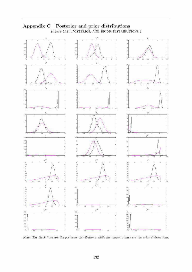
Appendix C Posterior and prior distributionsFigure C.1: Posterior and prior distributions I

2 3 4 5 6 7 8 90

0.2

0.4

0.6

0.8

1

ϕ

1 2 3 4 5 6 7 8 90

0.2

0.4

0.6

0.8

1

ϕ′

0.1 0.2 0.3 0.4 0.5 0.6 0.7 0.8 0.90

2

4

6

8

10

ν

0 0.1 0.2 0.3 0.4 0.5 0.6 0.7 0.80

2

4

6

8

10

ν ′

0.5 0.6 0.7 0.8 0.9 10

2

4

6

8

10

12

14

16

θ

0 0.2 0.4 0.6 0.8 1 1.20

2

4

6

8

10

ι

0.5 0.6 0.7 0.8 0.9 10

20

40

60

80

100

θw

0 0.2 0.4 0.6 0.8 1 1.20

5

10

15

20

25

30

35

ιw

0.5 0.6 0.7 0.8 0.9 10

10

20

30

40

50

φR

1.3 1.4 1.5 1.6 1.7 1.80

5

10

15

φπ

0.2 0.25 0.3 0.35 0.4 0.45 0.50

5

10

15

20

φy

0 1 2 3 4 50

2

4

6

8

10

φ

0 0.5 1 1.5 2 2.5 30

5

10

15

20

25

30

ψ

0.4 0.5 0.6 0.7 0.8 0.9 10

2

4

6

8

10

µ

0 0.2 0.4 0.6 0.8 1 1.20

5

10

15

20

ρG

0 0.2 0.4 0.6 0.8 1 1.20

1

2

3

4

5

6

7

8

ρtr

0 0.2 0.4 0.6 0.8 1 1.20

1

2

3

4

5

6

7

8

ρw

0 0.2 0.4 0.6 0.8 1 1.20

1

2

3

4

5

6

7

8

ρc

0 0.2 0.4 0.6 0.8 1 1.20

1

2

3

4

5

6

7

8

ρk

0 0.2 0.4 0.6 0.8 10

50

100

150

ρG,b

0 0.2 0.4 0.6 0.8 10

10

20

30

40

50

ρtr,b

0 0.2 0.4 0.6 0.8 10

10

20

30

40

50

60

ρw,b

0 0.2 0.4 0.6 0.8 10

20

40

60

80

100

ρc,b

0 0.2 0.4 0.6 0.8 10

5

10

15

20

25

30

35

40

ρk,b

Note: The black lines are the posterior distributions, while the magenta lines are the prior distributions.

132

Figure C.2: Posterior and prior distributions II

-0.25 -0.2 -0.15 -0.1 -0.05 0 0.05 0.1 0.150

2

4

6

8

10

12

14

16

ρG,y

-0.5 -0.4 -0.3 -0.2 -0.1 0 0.10

5

10

15

ρtr,y

-0.2 0 0.2 0.4 0.6 0.8 10

1

2

3

4

5

6

ρw,y

-0.1 0 0.1 0.2 0.3 0.4 0.5 0.6 0.70

5

10

15

20

25

30

ρc,y

-0.2 0 0.2 0.4 0.6 0.80

1

2

3

4

5

6

ρk,y

0.4 0.5 0.6 0.7 0.8 0.9 1 1.10

5

10

15

20

ρA

0.5 0.6 0.7 0.8 0.9 1 1.10

2

4

6

8

10

ρh

0.4 0.5 0.6 0.7 0.8 0.9 1 1.10

2

4

6

8

10

ρβ

0.4 0.5 0.6 0.7 0.8 0.9 1 1.10

5

10

15

20

25

30

ρN

0.4 0.5 0.6 0.7 0.8 0.9 1 1.10

50

100

150

200

250

300

350

ρW

0 0.01 0.02 0.03 0.04 0.05 0.060

200

400

600

800

1000

σA

-0.1 0 0.1 0.2 0.3 0.4 0.5 0.6 0.70

50

100

150

σh

0 0.01 0.02 0.03 0.04 0.05 0.060

50

100

150

200

250

300

σN

0 0.01 0.02 0.03 0.04 0.05 0.060

50

100

150

200

250

300

σW

0 0.01 0.02 0.03 0.04 0.05 0.060

500

1000

1500

σu

0 0.005 0.01 0.015 0.02 0.025 0.03 0.035 0.040

500

1000

1500

2000

2500

3000

3500

4000

σR

0 0.01 0.02 0.03 0.04 0.05 0.060

50

100

150

200

250

300

350

400

σβ

0 0.01 0.02 0.03 0.04 0.05 0.060

100

200

300

400

500

600

700

σg

0 0.01 0.02 0.03 0.04 0.05 0.060

50

100

150

200

σtr

0 0.01 0.02 0.03 0.04 0.05 0.060

50

100

150

200

250

300

350

στw

0 0.01 0.02 0.03 0.04 0.05 0.060

100

200

300

400

500

600

στ c

0 0.01 0.02 0.03 0.04 0.05 0.060

50

100

150

200

250

300

στk

×10-3

0 1 2 3 4 50

200

400

600

800

1000

1200

1400

1600

1800

Measurement error on πw

0 0.05 0.1 0.15 0.2 0.25 0.3 0.350

20

40

60

80

100

120

140

160

Measurement error on bG

Note: The black lines are the posterior distributions, while the magenta lines are the prior distributions.

133

Appendix D Figures and tablesD.1 Impulse response functions and tablesFigure D.1-D.6 are detailed plots of the impulse response functions in section 6.1:

Figure D.1: Impulse response functions to 1% increase in govern. spending

0

0

Baseline No collateral effect

0 5 10 15 20

-0.1

0

0.1

0.2

Output

0 5 10 15 20

-0.08

-0.06

-0.04

-0.02

0

Aggregate consumption

0 5 10 15 20

-0.08

-0.06

-0.04

-0.02

0

Cons. (patient)

0 5 10 15 20

-0.15

-0.1

-0.05

0

Cons. (impatient)

0 5 10 15 20

-0.2

-0.15

-0.1

-0.05

0

0.05

Unemployment

0 5 10 15 20

-0.05

0

0.05

0.1

0.15

0.2

Employment

0 5 10 15 20

-0.02

-0.01

0

0.01

0.02

Labor force

0 5 10 15 20

-0.025

-0.02

-0.015

-0.01

-0.005

0

Real wage

0 5 10 15 20

-0.2

-0.15

-0.1

-0.05

0

Investment

0 5 10 15 20

-0.1

0

0.1

0.2

Cap. utilization

0 5 10 15 20

-0.015

-0.01

-0.005

0

Price markup

0 5 10 15 20

-0.08

-0.06

-0.04

-0.02

0

House price

0 5 10 15 20

-0.04

-0.02

0

0.02

0.04

0.06

Housing (patient)

0 5 10 15 20

-0.4

-0.3

-0.2

-0.1

0

0.1

Mortgage debt

0 5 10 15 20

0

0.02

0.04

0.06

0.08

0.1

Inflation

0 5 10 15 20

0

0.02

0.04

0.06

0.08

0.1

Nominal interest rate

0 5 10 15 20

-0.01

-0.005

0

0.005

0.01

0.015

Exp. real interest rate

0 5 10 15 20

-0.5

0

0.5

1

1.5

Government spending

0 5 10 15 20

0

0.5

1

1.5

2

2.5

Government debt

0 5 10 15 20

0

0.1

0.2

0.3

Total distortionary taxes

0 5 10 15 20

-0.25

-0.2

-0.15

-0.1

-0.05

0

Transfers

0 5 10 15 20

0

0.05

0.1

0.15

0.2

Capital tax rate

0 5 10 15 20

0

0.02

0.04

0.06

0.08

Labor tax rate

0 5 10 15 20

0

0.005

0.01

0.015

VAT rate

Note: x-axis denotes quarters, while y-axis denotes percentage deviations from steady state (the y-axismeasures percentage point deviations from steady state for unemployment, inflation, nominal andexpected real interest rate, where the latter three are annualized).

134

D.1 Impulse response functions and tables

Figure D.2: Impulse response functions to a 1% decrease in VAT rate

0

0

Baseline No collateral effect

0 5 10 15 20

-0.01

0

0.01

0.02

0.03

Output

0 5 10 15 20

-0.01

0

0.01

0.02

0.03

0.04

Aggregate consumption

0 5 10 15 20

0

0.01

0.02

0.03

0.04

Cons. (patient)

0 5 10 15 20

-0.02

0

0.02

0.04

Cons. (impatient)

0 5 10 15 20

-0.03

-0.02

-0.01

0

0.01

Unemployment

0 5 10 15 20

-0.01

0

0.01

0.02

0.03

Employment

0 5 10 15 20

-2

-1

0

1

2×10

-3 Labor force

0 5 10 15 20

-2.5

-2

-1.5

-1

-0.5

0×10

-3 Real wage

0 5 10 15 20

-0.025

-0.02

-0.015

-0.01

-0.005

0

Investment

0 5 10 15 20

-0.02

-0.01

0

0.01

0.02

0.03

Cap. utilization

0 5 10 15 20

-2

-1.5

-1

-0.5

0×10

-3 Price markup

0 5 10 15 20

-8

-6

-4

-2

0

2×10

-3 House price

0 5 10 15 20

-10

-5

0

5×10

-3 Housing (patient)

0 5 10 15 20

-0.02

0

0.02

0.04

0.06

Mortgage debt

0 5 10 15 20

0

2

4

6

8×10

-3 Inflation

0 5 10 15 20

0

0.005

0.01

0.015

Nominal interest rate

0 5 10 15 20

-1

0

1

2

3

4×10

-3 Exp. real interest rate

0 5 10 15 20

-0.025

-0.02

-0.015

-0.01

-0.005

0

Government spending

0 5 10 15 20

0

0.1

0.2

0.3

Government debt

0 5 10 15 20

-0.2

-0.15

-0.1

-0.05

0

0.05

Total distortionary taxes

0 5 10 15 20

-0.03

-0.02

-0.01

0

Transfers

0 5 10 15 20

0

0.005

0.01

0.015

0.02

Capital tax rate

0 5 10 15 20

0

0.002

0.004

0.006

0.008

0.01

Labor tax rate

0 5 10 15 20

-0.08

-0.06

-0.04

-0.02

0

VAT rate

Note: x-axis denotes quarters, while y-axis denotes percentage deviations from steady state (the y-axismeasures percentage point deviations from steady state for unemployment, inflation, nominal andexpected real interest rate, where the latter three are annualized).

135

D.1 Impulse response functions and tables

Figure D.3: Impulse response functions to a 1% decrease in labor tax rate

0

0

Baseline No collateral effect

0 5 10 15 20

-0.04

-0.02

0

0.02

0.04

Output

0 5 10 15 20

-0.01

0

0.01

0.02

0.03

0.04

Aggregate consumption

0 5 10 15 20

0

0.005

0.01

0.015

0.02

Cons. (patient)

0 5 10 15 20

-0.05

0

0.05

0.1

0.15

0.2

Cons. (impatient)

0 5 10 15 20

-0.02

-0.01

0

0.01

0.02

0.03

Unemployment

0 5 10 15 20

-0.02

0

0.02

0.04

Employment

0 5 10 15 20

-0.02

0

0.02

0.04

0.06

Labor force

0 5 10 15 20

-8

-6

-4

-2

0×10

-3 Real wage

0 5 10 15 20

0

0.01

0.02

0.03

0.04

0.05

Investment

0 5 10 15 20

-0.06

-0.04

-0.02

0

0.02

0.04

Cap. utilization

0 5 10 15 20

-6

-4

-2

0

2×10

-3 Price markup

0 5 10 15 20

0

0.005

0.01

0.015

0.02

0.025

House price

0 5 10 15 20

-0.1

-0.05

0

0.05

Housing (patient)

0 5 10 15 20

-0.2

0

0.2

0.4

0.6

Mortgage debt

0 5 10 15 20

0

0.005

0.01

0.015

0.02

0.025

Inflation

0 5 10 15 20

-0.01

0

0.01

0.02

0.03

Nominal interest rate

0 5 10 15 20

-6

-4

-2

0×10

-3 Exp. real interest rate

0 5 10 15 20

-0.1

-0.08

-0.06

-0.04

-0.02

0

Government spending

0 5 10 15 20

0

0.2

0.4

0.6

0.8

1

Government debt

0 5 10 15 20

-0.6

-0.4

-0.2

0

0.2

Total distortionary taxes

0 5 10 15 20

-0.1

-0.08

-0.06

-0.04

-0.02

0

Transfers

0 5 10 15 20

0

0.02

0.04

0.06

Capital tax rate

0 5 10 15 20

-0.3

-0.2

-0.1

0

0.1

Labor tax rate

0 5 10 15 20

0

1

2

3

4×10

-3 VAT rate

Note: x-axis denotes quarters, while y-axis denotes percentage deviations from steady state (the y-axismeasures percentage point deviations from steady state for unemployment, inflation, nominal andexpected real interest rate, where the latter three are annualized).

136

D.1 Impulse response functions and tables

Figure D.4: Impulse response functions to a 1% decrease in capital tax rate

0

0

Baseline No collateral effect

0 5 10 15 20

-5

0

5

10

15

20×10

-3 Output

0 5 10 15 20

-0.02

-0.01

0

0.01

0.02

Aggregate consumption

0 5 10 15 20

-0.02

-0.01

0

0.01

0.02

Cons. (patient)

0 5 10 15 20

-0.06

-0.04

-0.02

0

Cons. (impatient)

0 5 10 15 20

-0.02

0

0.02

0.04

0.06

Unemployment

0 5 10 15 20

-0.06

-0.04

-0.02

0

0.02

Employment

0 5 10 15 20

-5

0

5

10×10

-3 Labor force

0 5 10 15 20

0

2

4

6

8×10

-3 Real wage

0 5 10 15 20

-0.06

-0.04

-0.02

0

0.02

0.04

Investment

0 5 10 15 20

-0.05

0

0.05

0.1

0.15

Cap. utilization

0 5 10 15 20

-0.02

0

0.02

0.04

0.06

0.08

Price markup

0 5 10 15 20

-0.02

-0.01

0

0.01

0.02

House price

0 5 10 15 20

0

0.01

0.02

0.03

0.04

Housing (patient)

0 5 10 15 20

-0.25

-0.2

-0.15

-0.1

-0.05

0

Mortgage debt

0 5 10 15 20

-0.03

-0.02

-0.01

0

0.01

Inflation

0 5 10 15 20

-0.015

-0.01

-0.005

0

Nominal interest rate

0 5 10 15 20

-0.01

0

0.01

0.02

0.03

Exp. real interest rate

0 5 10 15 20

-0.04

-0.03

-0.02

-0.01

0

Government spending

0 5 10 15 20

-0.2

0

0.2

0.4

0.6

Government debt

0 5 10 15 20

-0.3

-0.2

-0.1

0

0.1

Total distortionary taxes

0 5 10 15 20

-0.05

-0.04

-0.03

-0.02

-0.01

0

Transfers

0 5 10 15 20

-0.4

-0.3

-0.2

-0.1

0

0.1

Capital tax rate

0 5 10 15 20

0

0.005

0.01

0.015

Labor tax rate

0 5 10 15 20

0

0.5

1

1.5

2×10

-3 VAT rate

Note: x-axis denotes quarters, while y-axis denotes percentage deviations from steady state (the y-axismeasures percentage point deviations from steady state for unemployment, inflation, nominal andexpected real interest rate, where the latter three are annualized).

137

D.1 Impulse response functions and tables

Figure D.5: Impulse response functions to a 1% decrease in housing taxrate

0

0

Baseline No collateral effect

0 5 10 15 20

-4

-2

0

2

4

6×10

-3 Output

0 5 10 15 20

-2

0

2

4

6×10

-3 Aggregate consumption

0 5 10 15 20

0

1

2

3×10

-3 Cons. (patient)

0 5 10 15 20

-0.01

0

0.01

0.02

Cons. (impatient)

0 5 10 15 20

-8

-6

-4

-2

0

2×10

-3 Unemployment

0 5 10 15 20

-4

-2

0

2

4

6×10

-3 Employment

0 5 10 15 20

-3

-2

-1

0×10

-3 Labor force

0 5 10 15 20

-1

-0.8

-0.6

-0.4

-0.2

0×10

-3 Real wage

0 5 10 15 20

0

2

4

6

8×10

-3 Investment

0 5 10 15 20

-10

-5

0

5×10

-3 Cap. utilization

0 5 10 15 20

-10

-5

0

5×10

-4 Price markup

0 5 10 15 20

0

0.005

0.01

0.015

House price

0 5 10 15 20

-20

-15

-10

-5

0

5×10

-3 Housing (patient)

0 5 10 15 20

-0.05

0

0.05

0.1

0.15

Mortgage debt

0 5 10 15 20

-1

0

1

2

3

4×10

-3 Inflation

0 5 10 15 20

-1

0

1

2

3×10

-3 Nominal interest rate

0 5 10 15 20

-15

-10

-5

0

5×10

-4 Exp. real interest rate

0 5 10 15 20

-0.015

-0.01

-0.005

0

Government spending

0 5 10 15 20

0

0.05

0.1

0.15

0.2

Government debt

0 5 10 15 20

-0.15

-0.1

-0.05

0

0.05

Total distortionary taxes

0 5 10 15 20

-0.015

-0.01

-0.005

0

Transfers

0 5 10 15 20

0

0.002

0.004

0.006

0.008

0.01

Capital tax rate

0 5 10 15 20

0

1

2

3

4

5×10

-3 Labor tax rate

0 5 10 15 20

0

2

4

6

8×10

-4 VAT rate

Note: x-axis denotes quarters, while y-axis denotes percentage deviations from steady state (the y-axismeasures percentage point deviations from steady state for unemployment, inflation, nominal andexpected real interest rate, where the latter three are annualized).

138

D.1 Impulse response functions and tables

Figure D.6: Impulse response functions to a 1% increase in transfers

0

0

Baseline No collateral effect

0 5 10 15 20

-0.01

-0.005

0

0.005

0.01

Output

0 5 10 15 20

-5

0

5

10×10

-3 Aggregate consumption

0 5 10 15 20

0

1

2

3

4

5×10

-3 Cons. (patient)

0 5 10 15 20

-0.01

0

0.01

0.02

0.03

0.04

Cons. (impatient)

0 5 10 15 20

-15

-10

-5

0

5×10

-3 Unemployment

0 5 10 15 20

-5

0

5

10×10

-3 Employment

0 5 10 15 20

-5

-4

-3

-2

-1

0×10

-3 Labor force

0 5 10 15 20

-2

-1.5

-1

-0.5

0×10

-3 Real wage

0 5 10 15 20

0

0.005

0.01

0.015

Investment

0 5 10 15 20

-0.015

-0.01

-0.005

0

0.005

0.01

Cap. utilization

0 5 10 15 20

-15

-10

-5

0

5×10

-4 Price markup

0 5 10 15 20

0

2

4

6×10

-3 House price

0 5 10 15 20

-20

-15

-10

-5

0

5×10

-3 Housing (patient)

0 5 10 15 20

-0.05

0

0.05

0.1

Mortgage debt

0 5 10 15 20

0

2

4

6×10

-3 Inflation

0 5 10 15 20

0

2

4

6×10

-3 Nominal interest rate

0 5 10 15 20

-15

-10

-5

0

5×10

-4 Exp. real interest rate

0 5 10 15 20

-0.02

-0.015

-0.01

-0.005

0

Government spending

0 5 10 15 20

0

0.05

0.1

0.15

0.2

0.25

Government debt

0 5 10 15 20

0

0.005

0.01

0.015

0.02

0.025

Total distortionary taxes

0 5 10 15 20

0

0.5

1

1.5

Transfers

0 5 10 15 20

0

0.005

0.01

0.015

Capital tax rate

0 5 10 15 20

0

2

4

6

8×10

-3 Labor tax rate

0 5 10 15 20

0

0.2

0.4

0.6

0.8

1×10

-3 VAT rate

Note: x-axis denotes quarters, while y-axis denotes percentage deviations from steady state (the y-axismeasures percentage point deviations from steady state for unemployment, inflation, nominal andexpected real interest rate, where the latter three are annualized).

139

D.1 Impulse response functions and tables

Table 9: Impact multipliers for output

1 quarter 4 quarters 12 quarters 20 quarters

∆Yt+k

∆Gt0.94 0.47 -0.20 -0.32

[0.83, 1.06] [0.36, 0.59] [−0.27,−0.13] [−0.45,−0.21]∆Yt+k

−∆TCt

0.62 0.35 -0.23 -0.17

[0.50, 0.76] [0.22, 0.49] [−0.30,−0.17] [−0.29,−0.07]∆Yt+k

−∆TWt

0.25 0.19 -0.20 -0.14

[0.18, 0.34] [0.12, 0.27] [−0.27,−0.13] [−0.24,−0.07]∆Yt+k

−∆TKt

0.25 0.18 0.10 -0.00

[−0.03, 0.45] [0.09, 0.29] [−0.01, 0.29] [−0.05, 0.04]∆Yt+k

−∆THt

0.21 0.10 -0.16 -0.09

[0.17, 0.27] [0.08, 0.13] [−0.21, 0.13] [−0.13,−0.05]∆Yt+k

∆TTrt

0.29 0.22 -0.21 -0.18

[0.20, 0.40] [0.14, 0.34] [−0.27,−0.15] [−0.32,−0.09]

Note: The reported values are the means of the present value multipliers calculated for simulations ofthe model for 25,000 parameter vectors randomly drawn from the draws generated by the MH algorithm.The 5% and 95% percentiles are reported below in brackets.

140

D.2 Government spending with/without detailed fiscal block

D.2 Government spending with/without detailed fiscal block

Figure D.7: IRF to a 1% increase in government spending: Detailed fiscalsector (Baseline model) versus simplified fiscal sector

0Baseline Simplified fiscal sector

0 5 10 15 20

-0.1

0

0.1

0.2

Output

0 5 10 15 20

-0.15

-0.1

-0.05

0

Aggregate consumption

0 5 10 15 20

-0.15

-0.1

-0.05

0

Cons. (patient)

0 5 10 15 20

-0.2

-0.15

-0.1

-0.05

0

Cons. (impatient)

0 5 10 15 20

-0.2

-0.15

-0.1

-0.05

0

0.05

Unemployment

0 5 10 15 20

-0.05

0

0.05

0.1

0.15

0.2

Employment

0 5 10 15 20

-0.01

0

0.01

0.02

0.03

0.04

Labor force

0 5 10 15 20

-0.04

-0.03

-0.02

-0.01

0

Real wage

0 5 10 15 20

-0.4

-0.3

-0.2

-0.1

0

Investment

0 5 10 15 20

-0.1

0

0.1

0.2

Cap. utilization

0 5 10 15 20

-0.01

-0.008

-0.006

-0.004

-0.002

0

Price markup

0 5 10 15 20

-0.15

-0.1

-0.05

0

House price

0 5 10 15 20

-0.05

0

0.05

0.1

0.15

0.2

Housing (patient)

0 5 10 15 20

-1.5

-1

-0.5

0

0.5

Mortgage debt

0 5 10 15 20

0

0.05

0.1

0.15

Inflation

0 5 10 15 20

0

0.05

0.1

0.15

Nominal interest rate

0 5 10 15 20

-0.02

-0.01

0

0.01

0.02

0.03

Exp. real interest rate

0 5 10 15 20

0

0.5

1

1.5

Government spending

0 5 10 15 20

0

2

4

6

8

Government debt

0 5 10 15 20

-0.1

0

0.1

0.2

0.3

Total distortionary taxes

0 5 10 15 20

-0.8

-0.6

-0.4

-0.2

0

Transfers

0 5 10 15 20

0

0.05

0.1

0.15

0.2

Capital tax rate

0 5 10 15 20

0

0.02

0.04

0.06

0.08

0.1

Labor tax rate

0 5 10 15 20

0

0.005

0.01

0.015

VAT rate

Note: x-axis denotes quarters, while y-axis denotes percentage deviations from steady state (the y-axismeasures percentage point deviations from steady state for unemployment, inflation, nominal andexpected real interest rate, where the latter three are annualized).

141

D.3 Government spending under different φR’s

D.3 Government spending under different φR’s

Figure D.8: IRF to a 1% increase in government spending under differentφR

00.4Baseline,φ

R=0.91341 Low interest smoothing,φ

R=0.5 High interest smoothing,φ

R=0.99

0 5 10 15 20

-0.2

-0.1

0

0.1

0.2

0.3

Output

0 5 10 15 20

-0.15

-0.1

-0.05

0

0.05

Aggregate consumption

0 5 10 15 20

-0.15

-0.1

-0.05

0

0.05

Cons. (patient)

0 5 10 15 20

-0.2

-0.1

0

0.1

0.2

Cons. (impatient)

0 5 10 15 20

-0.4

-0.3

-0.2

-0.1

0

0.1

Unemployment

0 5 10 15 20

-0.1

0

0.1

0.2

0.3

Employment

0 5 10 15 20

-0.04

-0.02

0

0.02

0.04

Labor force

0 5 10 15 20

-0.03

-0.02

-0.01

0

Real wage

0 5 10 15 20

-0.4

-0.3

-0.2

-0.1

0

0.1

Investment

0 5 10 15 20

-0.2

-0.1

0

0.1

0.2

0.3

Cap. utilization

0 5 10 15 20

-15

-10

-5

0

5×10

-3 Price markup

0 5 10 15 20

-0.15

-0.1

-0.05

0

0.05

House price

0 5 10 15 20

-0.1

0

0.1

0.2

Housing (patient)

0 5 10 15 20

-1.5

-1

-0.5

0

0.5

Mortgage debt

0 5 10 15 20

0

0.05

0.1

0.15

Inflation

0 5 10 15 20

0

0.05

0.1

0.15

0.2

Nominal interest rate

0 5 10 15 20

-0.04

-0.02

0

0.02

0.04

0.06

Exp. real interest rate

0 5 10 15 20

-0.5

0

0.5

1

1.5

Government spending

0 5 10 15 20

0

1

2

3

Government debt

0 5 10 15 20

0

0.1

0.2

0.3

0.4

Total distortionary taxes

0 5 10 15 20

-0.3

-0.2

-0.1

0

Transfers

0 5 10 15 20

0

0.05

0.1

0.15

0.2

Capital tax rate

0 5 10 15 20

0

0.02

0.04

0.06

0.08

0.1

Labor tax rate

0 5 10 15 20

0

0.005

0.01

0.015

VAT rate

Note: x-axis denotes quarters, while y-axis denotes percentage deviations from steady state (the y-axismeasures percentage point deviations from steady state for unemployment, inflation, nominal andexpected real interest rate, where the latter three are annualized).

142

D.4 Government spending and monetary accommodation

D.4 Government spending and monetary accommodation

Figure D.9: IRF to a 1% increase in government spending under monetaryaccommodation

0

0

Monetary accommodation Baseline

0 5 10 15 20

-0.2

0

0.2

0.4

0.6

Output

0 5 10 15 20

-0.2

-0.1

0

0.1

0.2

Aggregate consumption

0 5 10 15 20

-0.1

-0.05

0

0.05

0.1

Cons. (patient)

0 5 10 15 20

-0.2

0

0.2

0.4

Cons. (impatient)

0 5 10 15 20

-0.6

-0.4

-0.2

0

0.2

Unemployment

0 5 10 15 20

-0.2

0

0.2

0.4

0.6

Employment

0 5 10 15 20

-0.06

-0.04

-0.02

0

0.02

Labor force

0 5 10 15 20

-0.04

-0.03

-0.02

-0.01

0

Real wage

0 5 10 15 20

-0.2

0

0.2

0.4

Investment

0 5 10 15 20

-0.1

0

0.1

0.2

0.3

0.4

Cap. utilization

0 5 10 15 20

-0.02

-0.015

-0.01

-0.005

0

Price markup

0 5 10 15 20

-0.1

-0.05

0

0.05

0.1

0.15

House price

0 5 10 15 20

-0.2

-0.1

0

0.1

Housing (patient)

0 5 10 15 20

-0.5

0

0.5

1

1.5

Mortgage debt

0 5 10 15 20

0

0.05

0.1

0.15

0.2

Inflation

0 5 10 15 20

0

0.05

0.1

0.15

0.2

Nominal interest rate

0 5 10 15 20

-0.06

-0.04

-0.02

0

0.02

Exp. real interest rate

0 5 10 15 20

0

0.5

1

1.5

Government spending

0 5 10 15 20

0

1

2

3

Government debt

0 5 10 15 20

0

0.2

0.4

0.6

Total distortionary taxes

0 5 10 15 20

-0.3

-0.2

-0.1

0

Transfers

0 5 10 15 20

0

0.05

0.1

0.15

0.2

Capital tax rate

0 5 10 15 20

0

0.02

0.04

0.06

0.08

0.1

Labor tax rate

0 5 10 15 20

0

0.005

0.01

0.015

VAT rate

Note: x-axis denotes quarters, while y-axis denotes percentage deviations from steady state (the y-axismeasures percentage point deviations from steady state for unemployment, inflation, nominal andexpected real interest rate, where the latter three are annualized).

143

D.5 Government spending and nominal wage rigidities

D.5 Government spending and nominal wage rigidities

Figure D.10: IRF to a 1% increase in government spending under differentnominal wage rigidities

0

0Low wage stickiness, θw

=0.2 Baseline, θw

= 0.904

0 5 10 15 20

-0.1

0

0.1

0.2

0.3

Output

0 5 10 15 20

-0.15

-0.1

-0.05

0

Aggregate consumption

0 5 10 15 20

-0.15

-0.1

-0.05

0

Cons. (patient)

0 5 10 15 20

-0.2

-0.1

0

0.1

Cons. (impatient)

0 5 10 15 20

-0.2

-0.15

-0.1

-0.05

0

0.05

Unemployment

0 5 10 15 20

-0.05

0

0.05

0.1

0.15

0.2

Employment

0 5 10 15 20

-0.02

0

0.02

0.04

Labor force

0 5 10 15 20

-0.1

0

0.1

0.2

0.3

Real wage

0 5 10 15 20

-0.4

-0.3

-0.2

-0.1

0

Investment

0 5 10 15 20

-0.1

0

0.1

0.2

0.3

0.4

Cap. utilization

0 5 10 15 20

-0.15

-0.1

-0.05

0

0.05

Price markup

0 5 10 15 20

-0.15

-0.1

-0.05

0

House price

0 5 10 15 20

-0.1

-0.05

0

0.05

0.1

Housing (patient)

0 5 10 15 20

-0.4

-0.2

0

0.2

0.4

Mortgage debt

0 5 10 15 20

0

0.05

0.1

0.15

0.2

Inflation

0 5 10 15 20

0

0.05

0.1

0.15

0.2

Nominal interest rate

0 5 10 15 20

-0.1

-0.05

0

0.05

Exp. real interest rate

0 5 10 15 20

0

0.5

1

1.5

Government spending

0 5 10 15 20

0

1

2

3

4

Government debt

0 5 10 15 20

0

0.1

0.2

0.3

0.4

Total distortionary taxes

0 5 10 15 20

-0.4

-0.3

-0.2

-0.1

0

Transfers

0 5 10 15 20

0

0.05

0.1

0.15

0.2

0.25

Capital tax rate

0 5 10 15 20

0

0.02

0.04

0.06

0.08

0.1

Labor tax rate

0 5 10 15 20

0

0.005

0.01

0.015

VAT rate

Note: x-axis denotes quarters, while y-axis denotes percentage deviations from steady state (the y-axismeasures percentage point deviations from steady state for unemployment, inflation, nominal andexpected real interest rate, where the latter three are annualized).

144