Fiscal Sustainability of Mexican Debt Decisions: Is Bad

Behavior Rewarded?

Carmina J. Quiroga

Dr. Heidi Jane Smith

Nacional o Subnacional

-5,000,000.0

5,000,000.0

15,000,000.0

25,000,000.0

35,000,000.0

45,000,000.0

55,000,000.0

65,000,000.0

75,000,000.0

85,000,000.0

2013 2014 2015 2016 2017

Deuda Federal y subnacional en México2013-2017 (milliones depesos)

Subnational Federal

0

5

10

15

20

25

30

2002 2003 2004 2005 2006 2007 2008 2009 2010 2011 2012 2013 2014 2015 2016

Incremento porcentual del saldo annual de la deudasubnacional2002-2016

Inflación anual acumulada % Aumento anual de la deuda

%

Si bien la deuda puedepotenciar el crecimiento de lospaíses (Blanchard, 2019), pocose ha hablado de los nivelesóptimos de endeudamientosubnacional en países endesarrollo.

0.0

20.0

40.0

60.0

80.0

100.0

Porcentaje de deuda que se paga a través de participaciones federales

(1994-2016)

Elaboración propia con datos de SHCP

• La LDFEM propone controleslegales de centralización paraatender el problema

• La regulación fiscal a través decontroles legales no reducía nivelesde deuda estatal por Velázquez(2006)

• Los topes fiscales ni controleslegales tienen ningún efecto sobreel endeudamiento municipal porSmith (2006)

• Debe ser el mercado el que reguleel sobreendeudamiento proponenKleeman & Teo (2014), favorecenla descentralización.

Centralización financiera y deuda en México

Entendiendo la sustentabilidad financieras como los niveles deendeudamiento tales que generen crecimiento económico suficientepara a) Pagar la deuda y los intereses generados & b) Aumentar elbienestar social,

¿Cómo impacta la centralización de las finanzas públicas en la

sustentabilidad financiera de los gobiernos subnacionales en México?

Pregunta de Investigación

Índices de sustentabilidad

• GASTO: cuidar la relación deuda/gasto y equilibrio presupuestarioMendoza y Oviedo (2004), Horne (1991), Croce y Juan-Ramón(2003)

• PROYECTIONES: Mantener la sustentabilidad en función de lasproyecciones de ingreso futuro. (Paunovic, 2005) , Mendoza y Oviedo(2003)

• TRIBUTARIO : Mantener la sustentabiidad con tributación suaveTalvi y Végh (2000)

[𝑫𝒆𝒖𝒅𝒂𝑷/𝒄𝒕/𝑷𝑰𝑩𝒑/𝒄𝒕

] ∗ ∅ − (𝑻𝒓𝒂𝒏𝒔𝒇𝒆𝒓𝒕 + 𝑰𝒎𝒑𝒕 − 𝑬𝒈𝒓𝒆𝒔𝒐𝒔𝒕)/𝝅𝒕 = 0

Pimary Gap, Blanchard (1990)

Sustainability Defined

“primary gap” proposed by Blanchard (1990) The most basic variation of this model is the following:

𝐷𝑒𝑏𝑡𝑡+1 = 𝐷𝑒𝑏𝑡𝑡 1 + 𝑟 − (𝐼𝑡−𝐺𝑡)

Where 𝐷𝑒𝑏𝑡𝑡+1 is the amount of acquired debt for the end of the period, 𝐷𝑒𝑏𝑡𝑡 is the accrued debt until the studied period, 𝑟 is the real interest rate and (𝐼𝑡−𝐺𝑡) is the budget balance (Income-Expenditure) of the state. From this equation the basic relation emerges for the measurement of financial sustainability:

𝐷𝑒𝑏𝑡

𝐺𝐷𝑃=(𝐼𝑡 − 𝐺𝑡)

𝑟 − 𝑔

Where g is the expected average economic growth in the long term. What measures this identity is the desirable level of the Debt/GDP, with regards to the conditions of income, expenditure, interest rates and economic growth.

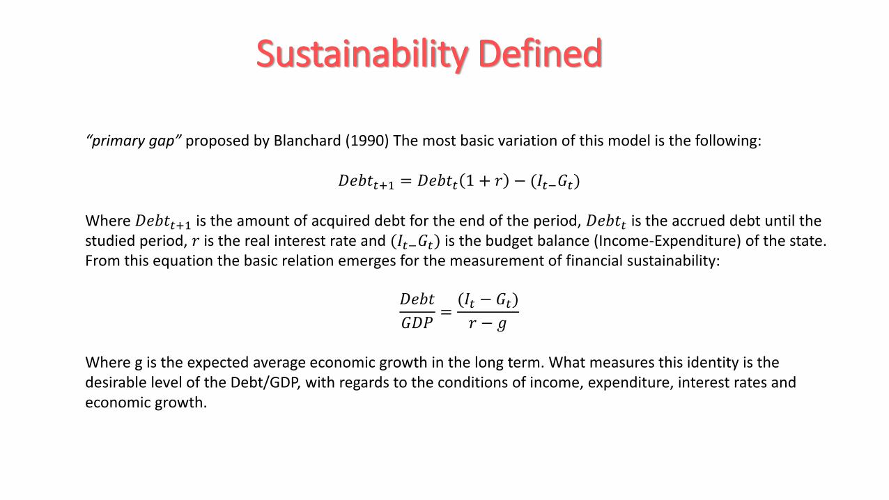
Brecha de Blanchard

-70000

-60000

-50000

-40000

-30000

-20000

-10000

0

10000

Comportamiento de la Brecha de Blanchard en municipios mexicanos 2000-2017

MAX PROMEDIO-45

-40

-35

-30

-25

-20

-15

-10

-5

0

5

2 0 0 02 0 0 12 0 0 22 0 0 32 0 0 42 0 0 52 0 0 62 0 0 72 0 0 82 0 0 92 0 1 02 0 1 12 0 1 22 0 1 32 0 1 42 0 1 52 0 1 62 0 1 7

MÁXIMOS HISTÓRICOS DE LA BRECHA DE BLANCHARD

MAX

Source: Own elaboration

BB= 𝜷𝟎 + 𝜷𝟏𝑻𝑶𝑺𝑹𝒑𝒄 +

𝜷𝟐𝑷𝒂𝒓𝒕𝒑𝒄 + 𝜷𝟑𝑨𝒑𝒐𝒓𝒕𝒑𝒄 +

𝜸𝒏(𝑽𝒂𝒓𝒊𝒂𝒃𝒍𝒆𝒔 𝒅𝒆 𝒄𝒐𝒏𝒕𝒓𝒐𝒍) +

𝜺

Modelo Fe para medir los efectos de la centralización fiscal

Data from 2000 to 2017. To calculate the Blanchard gap

yearly data of income and expenditure is used:

1. Sistema Estatal y Municipal de Bases de Datos,

SIMBAD

2. Instituto Nacional de Estadística y Geografía, INEGI

3. municipal GDP estimate is used, which the World Bank

presents in periods of 5 years (2000, 2005, 2010 y 2015)

4. data of accrued yearly inflation is used, for which the

yearly inflation is the same in all municipalities.

5. For the second model, municipal data presented by the

SHCP is used regarding the disaggregated municipal

debt by creditor type.

DescriptiveStatistics

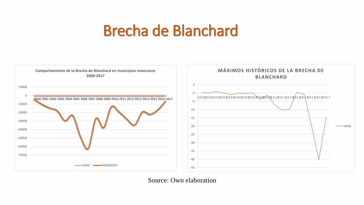
RESULTADOS

Variables Coef. Std. Err

TOSRpc 15.66587** (-1.04656)

Partpc -27.39125** (-0.82193)

Aportpc 18.75297** (0.648137)

Inperc 19645.61* (11714.3)

Inflation 628604.1 (530789.7)

_cons -9596.444 (25190.09)

*p<0.1, **p<0.05

The model is a regression with data from the panel with fixed effects, this is due to the Haussmann test showed that there is correlation between the errors.

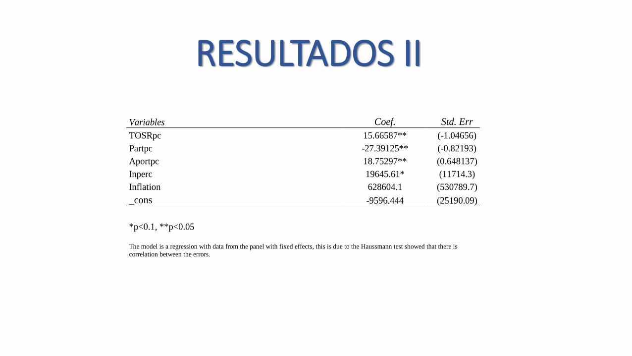
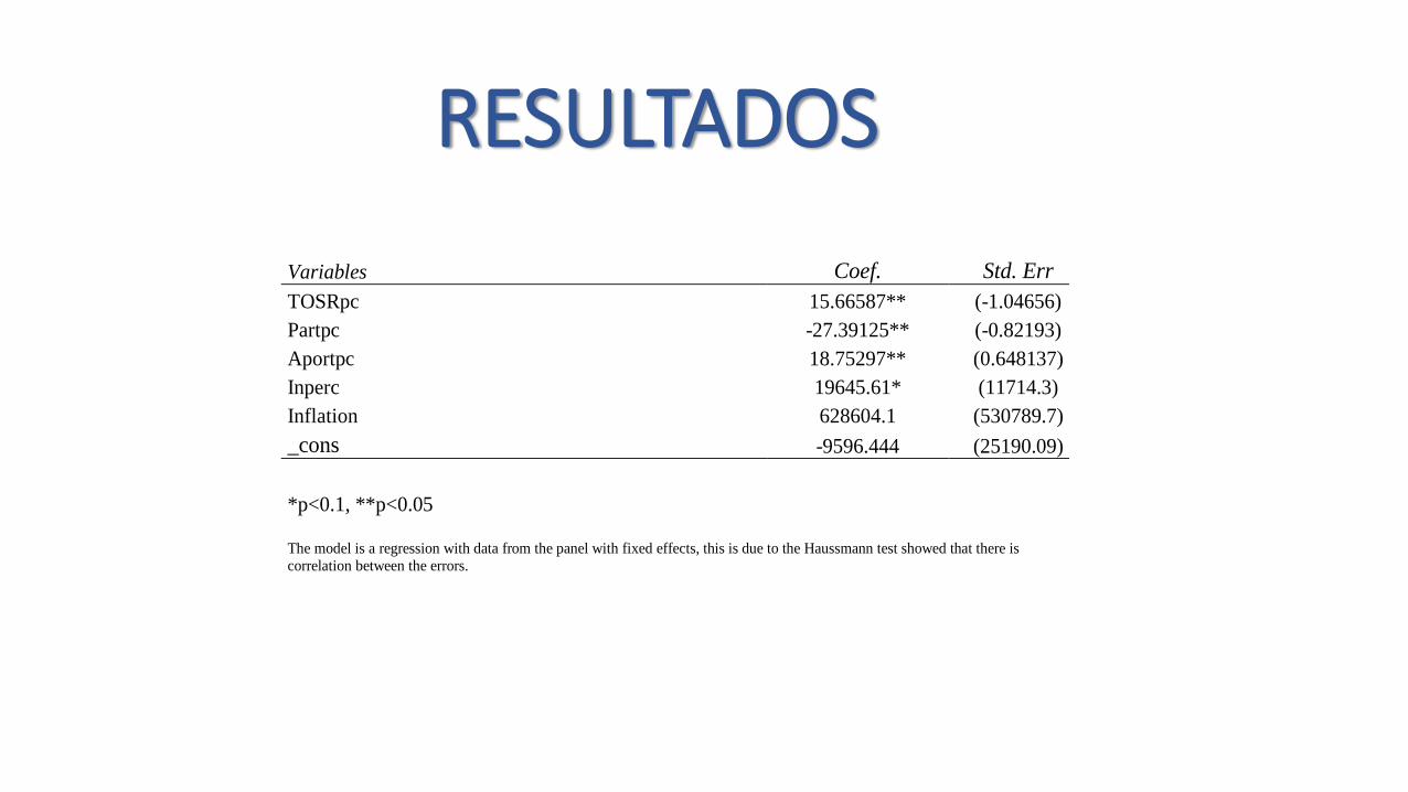
RESULTADOS II

Variables Coef. Std. Err

TOSRpc 15.66587** (-1.04656)

Partpc -27.39125** (-0.82193)

Aportpc 18.75297** (0.648137)

Inperc 19645.61* (11714.3)

Inflation 628604.1 (530789.7)

_cons -9596.444 (25190.09)

*p<0.1, **p<0.05

The model is a regression with data from the panel with fixed effects, this is due to the Haussmann test showed that there is correlation between the errors.

CONCLUSIONES

LDFEM

Pros Contras

Exige a los gobiernos

subnacionales ordenar

sus finanzas

Fortalece la centralización

financiera

Aumenta la

transparenciaRetroceso del federalismo

Exige homogeneización

de los procesos de deuda

Alarga el proceso de

adquisición

Promueve procesos

competitivos

Los parámetros de topes de

endeudamiento son

homogéneos y desfavorecen a

ciertas localidades dadas sus

características

Genera bases de datosContrae el mercado de deuda

gubernamental

o Falta de sofisticación del mercado de deuda subnacional

o Sobreendeudamiento por uso de instrumentos subóptimos

o La deuda está mal canalizada

o Las aportaciones pueden fungir como un elemento clave en el ejercicio del gasto

o La centralización desfavorece la sustentabilidad financiera