Embed Size (px)
Citation preview

1
Fisheries Management in Congested Waters: A Game-Theoretic Assessment of the East China Sea Michael Perry, [email protected] George Mason University, Department of Systems Engineering and Operations Research, Fairfax, VA, USA
1. Introduction
The East China Sea (ECS) is a congested maritime environment in the sense that fishermen from
multiple nations can access these waters with essentially equivalent operating costs. A journey
from China to Japan through the ECS, for example, can span less than 350 nautical miles, while
one from China to South Korea can span only 200 nautical miles. As a point of fact, fishermen
from each of these three nations have historically fished throughout the ECS under less
restrictive fisheries management regimes. Other congested maritime environments can of course
be identified, such as the South China Sea (SCS) where disputes exist between all major SCS
nations, but a distinguishing feature of the ECS is that legal agreements have been made on
paper for who’s allowed to fish where (Rosenberg 2005).
Despite such agreements between each China, South Korea, and Japan, illegal encroachments
persist in high volumes (Hsiao 2020). Writing this off as the behavior of self-interested
criminals is unsatisfactory, as state-led monitoring, controls, and surveillance (MCS) of fisheries
present cost-effective ways to deter illegal fishing, and yet MCS has been rated poorly among
ECS nations by the United Nations Food and Agricultural Organization (FAO) (Petrossian
2019). If these illegal encroachments were a true concern of the state, one would see more
investment in MCS. This paper provides a game-theoretic explanation for how rational state
policy can allow illegal encroachments to persist.

2
The paper analyzes a congested maritime environment using a game with two players, Blue and
Red. A key modeling framework is that despite legally defined fishing waters, nations can
tacitly allow illegal fishing by issuing excessive quotas in their own waters while letting
economic principles determine whether each fisherman will fish in Blue waters, Red waters, or
neither. Coupled with a standard fisheries model, this economic determination is influenced by
asymmetries in costs. While the proximities of nations are assumed to render operating costs
equivalent, asymmetries exist in the ECS on at least two accounts. Opportunity costs are the
most obvious asymmetry, as income opportunities in China differ greatly from South Korea and
Japan. The other source of asymmetry addressed is that arising from the deterrent effect of
patrol crafts. Not only can nations have differences in the quantity and quality of patrols, which
impose costs on illegal fishing, but a nation’s fishermen also differ in their ability to resist
patrols. The latter point has garnered significant attention in recent years with the rise of so-
called maritime militias; that is, fishermen armed with martial assets (often with state
sponsorship) such as water cannons and small arms that embolden them to fish in illegal waters.
As will be shown, the low-cost player can extract rent from the high-cost player’s waters by
issuing excessive quotas; one strategy the high-cost player can use to combat this is to issuing
excessive quotas herself, reducing the attractiveness of her waters to illegal fishermen and
creating a vicious circle of overfishing.
As already alluded, fisheries management entails more than issuing the “right” amount of quotas.
MCS measures are also essential to ensure fishermen are fishing only where allowed, catching
the allowable species in the allowed quantities, and so on. For the purposes of this paper, MCS

3
refers to such deterrent practices other than maritime patrols and includes measures such as port
inspections and vessel monitoring systems. It does not include sound practices for issuing
quotas, which is treated as a separate decision variable. The poorly-rated MCS observed in the
ECS can also be explained through strategic interaction in a congested environment. It’s seen
that even if MCS is a cost-effective deterrent of illegal fishing in the single-state context, once a
second player is introduced the incentive to invest in MCS vanishes.
A critical component in the analysis is that each player can behave against the norms of agreed
upon fishing rights while maintaining plausible deniability. For example, a country, say China,
cannot explicitly authorize fishermen to fish in South Korean waters, as if this were discovered
the political consequences would be unacceptable. This assertion is consistent with observed
behavior as China has historically punished its fishermen caught in South Korean waters (Zhang
2016). Likewise, if it were discovered China were knowingly letting fish caught in South
Korean waters in through its ports, the consequences would be unacceptable. It might be asked,
then, what is to be done, if an agreement is already on paper but countries nonetheless tacitly
violate it? To address this, the paper assesses what enforceable policy on fishing quotas can be
implemented to improve each player’s utility. Such a policy involves an observable agreement
on legal fishing levels, including legally allowed fishing by one player in the other’s waters, as
well as mutually observable MCS regimes. Unsurprisingly, the low-cost player, either by virtue
of low opportunity costs or strong patrols and maritime militias, has leverage in negotiating such
an enforceable policy. However, it’s found that in many situations only a reasonable amount of
legally allowed fishing by the low-cost player in the high-cost player’s waters can lead to a

4
significant and balanced benefit for each, and thus there’s likely a politically amenable solution
to improve fisheries management in the ECS.
The remainder of the paper is structured as follows. Section 2 reviews the literature on fisheries
management in the ECS as it pertains to illegal fishing, game theoretic models of fisheries, and
the deterrent effects of maritime law enforcement on illegal fishing. Section 3 describes a model
for the ECS as a two-player game where each player owns a specified number of fisheries; this
includes a subgame to determine where fishermen with quotas will fish. Section 4 derives
analytical results for the case when each player owns a single fishery, and examples are
presented for each the single- and multi-fishery cases. Section 5 concludes and comments on
future work. Two appendices are provided with mathematical proofs and solution algorithms for
the game.
2. Literature Review
Bilateral agreements delineating fishing rights in the ECS began to take form in the late 1990s,
delineating regions that would fall under the jurisdiction of particular states as well as jointly
managed areas. These agreements have also included provisions for legal fishing by one country
in the waters of another (Rosenberg 2005; Hsiao 2020). However, these agreements are not fully
cooperative in the sense that they haven’t set limits on domestic fishing; that is, a bilateral
agreement between China and South Korea may specify legal Chinese fishing levels in South
Korean waters, but not legal Chinese levels in Chinese waters. This oversight has led to
overfishing, and is perhaps the cause of current cutbacks on legally allowed foreign fishing
(Yonhap News 2020). Despite these agreements, illegal encroachments persist in large numbers.
An estimated 29,600 instances of Chinese fishing vessels entering South Korean waters occurred
5
in the second half of 2014 alone. Further, and in support of the assertion states may only tacitly
encourage illegal fishing but not outright allow it, Chinese officials have taken punitive action
against its illegal fishermen when detained by South Korea and other countries (Zhang 2016).
Analyzing these disputes has been complicated by the rise of maritime militias, the most well-
studied of which is the Chinese Maritime Militia. These militias are fishermen who’ve been
equipped with martial assets such as small arms and water cannons, generally through state-
sponsorship, to oppose other nation’s fishermen and patrol craft (Erickson and Kennedy 2016;
Zhang and Bateman 2017; Perry 2020). In the most extreme cases, interactions between
fishermen and maritime law enforcement has led to the loss of life on both sides (China Power
Team 2020; Park 2020).
A key tool for addressing illegal encroachments, and illegal fishing in general, is monitoring,
controls, and surveillance (MCS), which includes measures such as inspections at ports of entry,
onboard observers to monitor fishing activities, and satellite systems to track vessels (Pitcher,
Kalikoski, and Pramod 2006). The definition of MCS also often includes the issuance of quotas,
but quotas issuance is treated separately in this paper. Empirical studies have shown MCS to be
an effective deterrent to illegal fishing, and while costs can vary widely irrespective of MCS
quality its generally viewed as a cost-effective tool (Petrossian 2015; Mangin et al. 2018).
Fisheries management experts have, nonetheless, rated MCS practices among ECS nations as
below average (Petrossian 2019). Interestingly, studies have also found more generally that
fisheries management tends to be weaker when nearby states are also not adhering to best
practices, lending credence to the modeled results in this paper for congested maritime
environments (Borsky and Raschky 2011).

6
From a modeling perspective fisheries disputes have often been studied through game theory. In
the well-studied problem of two or more players allocating quotas in the same fishery, models
have shown overfishing will occur both when considering discounted payoffs and not. When
accounting for asymmetric costs a player’s utilities are seen to increase as another’s costs
increase (Grønbæk et al. 2020). While related to the findings of this paper, the distinction is the
model presented here considers multiple fisheries with legal definitions of who’s allowed to fish
in each, introducing a criminological element into the analysis. Models have accounted for
additional complicating factors such as multiple interacting species (Fischer and Mirman 1996),
coalition forming in many player games (Long and Flaaten 2011), and uncertainty in stock levels
and growth (Miller and Nkuiya 2016), to name a few. Models have also been used to optimize
patrol strategies to combat illegal fishing. These models discretize a nation’s waters and
consider two players, the state and illegal fishermen, who must determine how to deploy patrols
and where to attempt illegal fishing, respectively. Factors such as heterogeneous illegal
fishermen types, bounded rationality, and repeated play have all been incorporated (Fang, Stone,
and Tambe 2015; Brown, Haskell, and Tambe 2014). What has not been considered is situations
with multiple states competing over resources utilizing either state-sponsored or tacitly
encouraged illegal fishing.
Regarding the economics of illegal fishing, researches have assessed the annual dollar amount of
illegally caught fish to be between $10-$23.5 billion (Petrossian 2019). In addition to MCS,
empirical studies have found the number of patrol craft per 100,000 square kilometers to be a
significant explainer of illegal fishing (Petrossian 2015). Deterrence has also been analyzed at
7
the agent-level, where studies have shown fishermen do indeed rationalize their illegal fishing by
pointing out the risks and costs associated with being caught don’t outweigh the benefits (King
and Sutinen 2010; Kuperan and Sutinen 1998; Nielsen and Mathiesen 2003). Lastly, note a gap
in the empirical literature exists in understanding the impact of maritime militias on the
willingness to fish illegally; while maritime militias have been studied extensively, no empirical
evidence exists to quantify their impact.
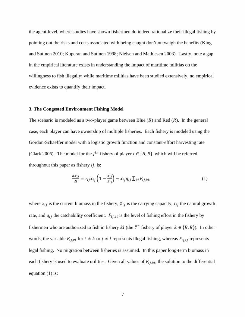
3. The Congested Environment Fishing Model
The scenario is modeled as a two-player game between Blue (𝐵𝐵) and Red (𝑅𝑅). In the general
case, each player can have ownership of multiple fisheries. Each fishery is modeled using the
Gordon-Schaeffer model with a logistic growth function and constant-effort harvesting rate
(Clark 2006). The model for the 𝑗𝑗𝑡𝑡ℎ fishery of player 𝑖𝑖 ∈ {𝐵𝐵,𝑅𝑅}, which will be referred
throughout this paper as fishery 𝑖𝑖𝑗𝑗, is:
𝑑𝑑𝑥𝑥𝑖𝑖𝑖𝑖𝑑𝑑𝑡𝑡
= 𝑟𝑟𝑖𝑖𝑖𝑖𝑥𝑥𝑖𝑖𝑖𝑖 �1 − 𝑥𝑥𝑖𝑖𝑖𝑖𝑍𝑍𝑖𝑖𝑖𝑖� − 𝑥𝑥𝑖𝑖𝑖𝑖𝑞𝑞𝑖𝑖𝑖𝑖 ∑ 𝐹𝐹𝑖𝑖𝑖𝑖,𝑘𝑘𝑘𝑘𝑘𝑘𝑘𝑘 , (1)
where 𝑥𝑥𝑖𝑖𝑖𝑖 is the current biomass in the fishery, 𝑍𝑍𝑖𝑖𝑖𝑖 is the carrying capacity, 𝑟𝑟𝑖𝑖𝑖𝑖 the natural growth
rate, and 𝑞𝑞𝑖𝑖𝑖𝑖 the catchability coefficient. 𝐹𝐹𝑖𝑖𝑖𝑖,𝑘𝑘𝑘𝑘 is the level of fishing effort in the fishery by
fishermen who are authorized to fish in fishery 𝑘𝑘𝑘𝑘 (the 𝑘𝑘𝑡𝑡ℎ fishery of player 𝑘𝑘 ∈ {𝐵𝐵,𝑅𝑅}). In other
words, the variable 𝐹𝐹𝑖𝑖𝑖𝑖,𝑘𝑘𝑘𝑘 for 𝑖𝑖 ≠ 𝑘𝑘 or 𝑗𝑗 ≠ 𝑘𝑘 represents illegal fishing, whereas 𝐹𝐹𝑖𝑖𝑖𝑖,𝑖𝑖𝑖𝑖 represents
legal fishing. No migration between fisheries is assumed. In this paper long-term biomass in
each fishery is used to evaluate utilities. Given all values of 𝐹𝐹𝑖𝑖𝑖𝑖,𝑘𝑘𝑘𝑘, the solution to the differential
equation (1) is:

8
𝑥𝑥𝑖𝑖𝑖𝑖 = 𝑍𝑍𝑖𝑖𝑖𝑖 �1 −𝑞𝑞𝑖𝑖𝑖𝑖 ∑ 𝐹𝐹𝑖𝑖𝑖𝑖,𝑘𝑘𝑘𝑘𝑘𝑘𝑘𝑘
𝑟𝑟𝑖𝑖𝑖𝑖�. (2)
To reiterate the key modeling framework, Blue and Red’s national strategy merely determines
how many fishing quotas are allocate in their respective fisheries, denoted 𝐹𝐹𝑘𝑘𝑘𝑘 for each fishery
𝑘𝑘𝑘𝑘. It’s assumed that without any explicit instruction from the state, individual fishermen with
quotas decide where to fish based on economic principles. The variables 𝐹𝐹𝑖𝑖𝑖𝑖,𝑘𝑘𝑘𝑘 will be
determined via a subgame to be detailed momentarily.
An individual fishermen’s revenue is a function of biomass. Denoting the price of fish farmed
from fishery 𝑖𝑖𝑗𝑗 as 𝑝𝑝𝑖𝑖𝑖𝑖, the revenue earned by a fisherman in this fishery is 𝑝𝑝𝑖𝑖𝑖𝑖𝑞𝑞𝑖𝑖𝑖𝑖𝑥𝑥𝑖𝑖𝑖𝑖. That
fishermen’s rent is determined by subtracting out costs, which obviously includes operational
costs, but also asymmetric opportunity costs and costs imposed through the efficacy of maritime
patrols to deter illegal fishing. It’s assumed all fisheries are in close enough proximity such that
operating costs are the same in each and for each player. In sum, the costs for a fisherman to fish
in 𝑖𝑖𝑗𝑗 when he’s legally authorized to fish in 𝑘𝑘𝑘𝑘 is defined as follows:
𝑐𝑐𝑖𝑖𝑖𝑖,𝑘𝑘𝑘𝑘 = � 𝑐𝑐𝑘𝑘, if 𝑖𝑖 = 𝑘𝑘 and 𝑗𝑗 = 𝑘𝑘𝑐𝑐𝑘𝑘 + 𝛽𝛽𝑘𝑘𝑃𝑃𝑖𝑖 + 𝛽𝛽𝑚𝑚𝑚𝑚𝑘𝑘, otherwise , (3)
where 𝑐𝑐𝑘𝑘 is the combined operating and opportunity costs for fishermen from country 𝑘𝑘, 𝑃𝑃𝑖𝑖 is the
number of patrol craft employed per 100,000 square kilometers by country 𝑖𝑖, and 𝑚𝑚𝑘𝑘 is the level
of MCS used in country 𝑘𝑘. The coefficient 𝛽𝛽𝑚𝑚 represents the deterrent effect of MCS on illegal
fishing and is assumed constant for both players. 𝛽𝛽𝑘𝑘, in contrast, is the deterrent effect of patrols
and is allowed to vary between players. This reflects differing levels of maritime militias among

9
ECS nations. Considering these costs, the rent earned by a fisherman is 𝜋𝜋𝑖𝑖𝑖𝑖,𝑘𝑘𝑘𝑘 = 𝑝𝑝𝑖𝑖𝑖𝑖𝑞𝑞𝑖𝑖𝑖𝑖𝑥𝑥𝑖𝑖𝑖𝑖 −
𝑐𝑐𝑖𝑖𝑖𝑖,𝑘𝑘𝑘𝑘.
Total utilities realized by Blue and Red, 𝑢𝑢𝐵𝐵 and 𝑢𝑢𝑅𝑅, are the sum total of rents collected by their
nation’s fishermen, minus expenditures on MCS. MCS costs are modeled as a function of the
level of MCS used; the flexible form 𝑎𝑎1𝑚𝑚𝑘𝑘𝑎𝑎2 is used, where 𝑎𝑎1 and 𝑎𝑎2 are constants. The level of
patrols is treated as a given constant rather than a decision variable, as in practice many other
considerations affect investment in patrol craft; for instance, port security, detection of human
trafficking, and search and rescue operations, to name a few applications. The utility functions
for Blue and Red are therefore:
𝑢𝑢𝐵𝐵 = ∑ ∑ 𝜋𝜋𝑖𝑖𝑖𝑖,𝐵𝐵𝑘𝑘𝐵𝐵𝑘𝑘𝑖𝑖𝑖𝑖 − 𝑎𝑎1𝑚𝑚𝐵𝐵𝑎𝑎2 (4)
𝑢𝑢𝑅𝑅 = ∑ ∑ 𝜋𝜋𝑖𝑖𝑖𝑖,𝑅𝑅𝑘𝑘𝑅𝑅𝑘𝑘𝑖𝑖𝑖𝑖 − 𝑎𝑎1𝑚𝑚𝑅𝑅𝑎𝑎2. (5)
By solving a subgame for the values of 𝐹𝐹𝑖𝑖𝑖𝑖,𝑘𝑘𝑘𝑘, these utility functions collapse into expressions of
the players’ overall decision variables (𝐹𝐹𝐵𝐵𝑘𝑘, 𝑚𝑚𝐵𝐵, 𝐹𝐹𝑅𝑅𝑘𝑘, and 𝑚𝑚𝑅𝑅).
3.1. Subgame for Levels of Fishing in Each Fishery
A state-issued fishing quota gives fishermen the legal right to bring fish into the country of issue.
States cannot explicitly direct fishermen to fish illegally; the decision on where to fish in a
congested environment is therefore left to the fishermen, a choice which will be made based on
economic principles. Elementally, the following must hold for a fishermen’s choice to be
economically rational: (i) a fishermen will use a quotas iff he can earn nonnegative rent; (ii) if
he’s fishing in fishery 𝑖𝑖𝑗𝑗, he must be earning at least as much rent as he could earn in any other
10
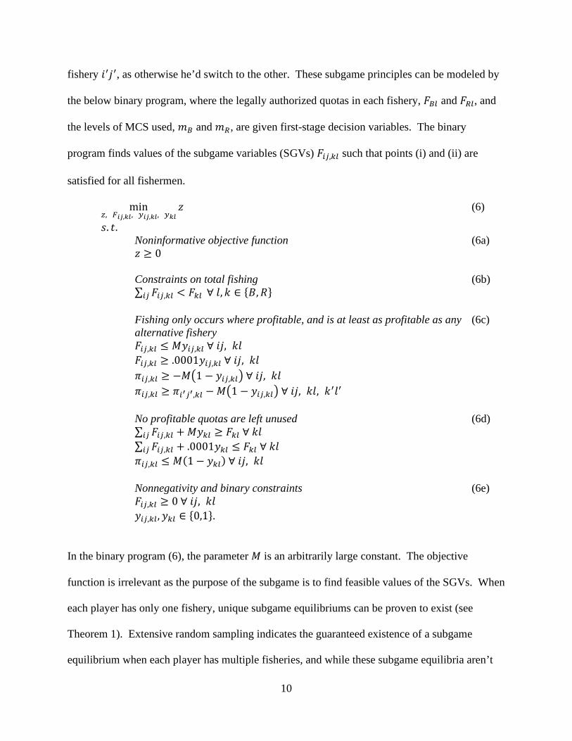
fishery 𝑖𝑖′𝑗𝑗′, as otherwise he’d switch to the other. These subgame principles can be modeled by
the below binary program, where the legally authorized quotas in each fishery, 𝐹𝐹𝐵𝐵𝑘𝑘 and 𝐹𝐹𝑅𝑅𝑘𝑘, and
the levels of MCS used, 𝑚𝑚𝐵𝐵 and 𝑚𝑚𝑅𝑅, are given first-stage decision variables. The binary
program finds values of the subgame variables (SGVs) 𝐹𝐹𝑖𝑖𝑖𝑖,𝑘𝑘𝑘𝑘 such that points (i) and (ii) are
satisfied for all fishermen.
min𝑧𝑧, 𝐹𝐹𝑖𝑖𝑖𝑖,𝑘𝑘𝑘𝑘, 𝑦𝑦𝑖𝑖𝑖𝑖,𝑘𝑘𝑘𝑘, 𝑦𝑦𝑘𝑘𝑘𝑘
𝑧𝑧 (6)
𝑠𝑠. 𝑡𝑡. Noninformative objective function (6a) 𝑧𝑧 ≥ 0 Constraints on total fishing (6b) ∑ 𝐹𝐹𝑖𝑖𝑖𝑖,𝑘𝑘𝑘𝑘 < 𝐹𝐹𝑘𝑘𝑘𝑘𝑖𝑖𝑖𝑖 ∀ 𝑘𝑘,𝑘𝑘 ∈ {𝐵𝐵,𝑅𝑅} Fishing only occurs where profitable, and is at least as profitable as any (6c) alternative fishery 𝐹𝐹𝑖𝑖𝑖𝑖,𝑘𝑘𝑘𝑘 ≤ 𝑀𝑀𝑦𝑦𝑖𝑖𝑖𝑖,𝑘𝑘𝑘𝑘 ∀ 𝑖𝑖𝑗𝑗, 𝑘𝑘𝑘𝑘 𝐹𝐹𝑖𝑖𝑖𝑖,𝑘𝑘𝑘𝑘 ≥ .0001𝑦𝑦𝑖𝑖𝑖𝑖,𝑘𝑘𝑘𝑘 ∀ 𝑖𝑖𝑗𝑗, 𝑘𝑘𝑘𝑘 𝜋𝜋𝑖𝑖𝑖𝑖,𝑘𝑘𝑘𝑘 ≥ −𝑀𝑀�1 − 𝑦𝑦𝑖𝑖𝑖𝑖,𝑘𝑘𝑘𝑘� ∀ 𝑖𝑖𝑗𝑗, 𝑘𝑘𝑘𝑘 𝜋𝜋𝑖𝑖𝑖𝑖,𝑘𝑘𝑘𝑘 ≥ 𝜋𝜋𝑖𝑖′𝑖𝑖′,𝑘𝑘𝑘𝑘 − 𝑀𝑀�1 − 𝑦𝑦𝑖𝑖𝑖𝑖,𝑘𝑘𝑘𝑘� ∀ 𝑖𝑖𝑗𝑗, 𝑘𝑘𝑘𝑘, 𝑘𝑘′𝑘𝑘′ No profitable quotas are left unused (6d) ∑ 𝐹𝐹𝑖𝑖𝑖𝑖,𝑘𝑘𝑘𝑘𝑖𝑖𝑖𝑖 + 𝑀𝑀𝑦𝑦𝑘𝑘𝑘𝑘 ≥ 𝐹𝐹𝑘𝑘𝑘𝑘 ∀ 𝑘𝑘𝑘𝑘 ∑ 𝐹𝐹𝑖𝑖𝑖𝑖,𝑘𝑘𝑘𝑘𝑖𝑖𝑖𝑖 + .0001𝑦𝑦𝑘𝑘𝑘𝑘 ≤ 𝐹𝐹𝑘𝑘𝑘𝑘 ∀ 𝑘𝑘𝑘𝑘 𝜋𝜋𝑖𝑖𝑖𝑖,𝑘𝑘𝑘𝑘 ≤ 𝑀𝑀(1 − 𝑦𝑦𝑘𝑘𝑘𝑘) ∀ 𝑖𝑖𝑗𝑗, 𝑘𝑘𝑘𝑘 Nonnegativity and binary constraints (6e) 𝐹𝐹𝑖𝑖𝑖𝑖,𝑘𝑘𝑘𝑘 ≥ 0 ∀ 𝑖𝑖𝑗𝑗, 𝑘𝑘𝑘𝑘 𝑦𝑦𝑖𝑖𝑖𝑖,𝑘𝑘𝑘𝑘, 𝑦𝑦𝑘𝑘𝑘𝑘 ∈ {0,1}.
In the binary program (6), the parameter 𝑀𝑀 is an arbitrarily large constant. The objective
function is irrelevant as the purpose of the subgame is to find feasible values of the SGVs. When
each player has only one fishery, unique subgame equilibriums can be proven to exist (see
Theorem 1). Extensive random sampling indicates the guaranteed existence of a subgame
equilibrium when each player has multiple fisheries, and while these subgame equilibria aren’t

11
guaranteed to be unique in general, they are unique at all equilibrium points for the overall game
found in Section 4.2. An analytical formula for the subgame equilibrium can be found in the
one-fishery case. These results are formalized in Theorems 1 and 2.
Theorem 1. Existence of a unique subgame equilibrium.
When Blue and Red each own only one fishery, any instantiation of the game’s
parameters and choice of the overall game’s decision variables yields a unique
subgame equilibrium.
Proof. See Appendix A.
Theorem 2. Formulae for the unique subgame equilibrium via a partitioning of
the parameter and decision space.
Again assume Blue and Red each own one fishery. The parameter and decision
variable space can be partitioned, such that in each region of the partition analytical
formulae exist for the subgame variables.
Proof. See Appendix A.
4. Examples
4.1. One Fishery per Player
Because each player has only owns one fishery, subscripts 𝑖𝑖1,𝑘𝑘1 are replaced with 𝑖𝑖,𝑘𝑘, and 𝑘𝑘1 is
replaced by 𝑘𝑘, for 𝑖𝑖,𝑘𝑘 ∈ {𝐵𝐵,𝑅𝑅}. This most basic instantiation of the model is sufficient to
understand why nations overfish, and why illegal encroachments persist, in a congested
environment. In addition to the analytical results in Theorems 1 and 2, when each player has
only one fishery it can be proven 𝑚𝑚𝐵𝐵 = 0 is always an optimal response for Blue, as is 𝑚𝑚𝑅𝑅 = 0

12
for Red. Thus, Blue and Red’s utility functions become quadratic functions of only 𝐹𝐹𝐵𝐵 and 𝐹𝐹𝑅𝑅,
where the quadratic form comes from the fact SGVs turn out to be linear in 𝐹𝐹𝐵𝐵 and 𝐹𝐹𝑅𝑅. This
result is formalized in Theorem 3, which implies MCS can be ignored in the one-fishery case.
It’s worth recalling the definition of MCS used in this paper: measures taken to ensure fishing is
occurring where allowed, other than patrols. In other words, 𝑚𝑚𝐵𝐵 = 𝑚𝑚𝑅𝑅 = 0 still allows for some
degree of strong fisheries management, such as strictly managed quota systems, restrictions on
access to fishing gear, and patrols. Not using MCS amounts to giving fishermen with a legal
quota a free pass to bring fishermen in through ports, irrespective of where it was caught.
Theorem 3
Assume Blue and Red each own one fishery. For a given strategy of the other player,
responding with 𝑚𝑚𝑘𝑘 > 0 can yield at most equivalent utility as using 𝑚𝑚𝑘𝑘 = 0. If costs of
MCS are nonzero, then 𝑚𝑚𝑘𝑘 > 0 yields strictly less utility than 𝑚𝑚𝑘𝑘 = 0.
Proof. See Appendix A.
Theorems 1, 2, and 3 make it relatively straightforward to find an equilibrium for the overall
game, allowing for thorough comparative statics. Because the form of the subgame equilibrium
depends on which section of the decision space the players’ decisions, 𝐹𝐹𝐵𝐵 and 𝐹𝐹𝑅𝑅, place the game
in, the players’ utilities likewise depend on this. The key to finding an equilibrium is to find
distinct intervals for 𝐹𝐹𝐵𝐵 where Red’s optimal response is a non-piecewise function of 𝐹𝐹𝐵𝐵, and
distinct intervals for 𝐹𝐹𝑅𝑅 where Blue’s optimal response is a non-piecewise function of 𝐹𝐹𝑅𝑅, and
finally seek pairs of intervals for 𝐹𝐹𝐵𝐵 and 𝐹𝐹𝑅𝑅 where the players’ optima intersect. Algorithm B1 in
Appendix B details how the required intervals are found, and the concept is illustrated in Figure

13
1. In this illustration, an equilibrium exists at (𝐹𝐹𝐵𝐵,𝐹𝐹𝑅𝑅) = (878, 1193), where the solid grey and
black lines intersect.
Fig. 1. Intervals where optimal responses are non-piecewise. Note. Grey and black dashed lines demarcate intervals where Blue and Red’s optimal responses are non-piecewise, respectively.
An important point is that an equilibrium isn’t guaranteed to exist for the overall game.
Comparative statics are performed in the following example, so in cases where an equilibrium
doesn’t exist the point that minimizes the value of �𝑢𝑢𝐵𝐵∗ (𝐹𝐹𝑅𝑅) − 𝑢𝑢𝐵𝐵(𝐹𝐹𝐵𝐵,𝐹𝐹𝑅𝑅)�2
+ �𝑢𝑢𝑅𝑅∗ (𝐹𝐹𝐵𝐵) −
𝑢𝑢𝑅𝑅(𝐹𝐹𝐵𝐵,𝐹𝐹𝑅𝑅)�2 is used in its place, where 𝑢𝑢𝐵𝐵∗ (𝐹𝐹𝑅𝑅) and 𝑢𝑢𝑅𝑅∗ (𝐹𝐹𝐵𝐵) are the optimal utilities Blue and
Red can earn when responding to 𝐹𝐹𝑅𝑅 and 𝐹𝐹𝐵𝐵, respectively. This point is easy to find given the
information encapsulated in Algorithm B1; one simply iterates through the distinct regions where
each 𝑢𝑢𝐵𝐵∗ (𝐹𝐹𝑅𝑅) and 𝑢𝑢𝑅𝑅∗ (𝐹𝐹𝐵𝐵) are non-piecewise and solves a constrained polynomial optimization.
In this paper the COBYLA method was used (Powell 1998).
4.1.1. Example 1.
Consider the following parameter values, where carrying capacities are measured in millions of
metric tons and prices are USD per million metric tons:
𝑍𝑍𝐵𝐵 = 𝑍𝑍𝑅𝑅 = 2, 𝑟𝑟𝐵𝐵 = 𝑟𝑟𝑅𝑅 = .4, 𝑞𝑞𝐵𝐵 = 𝑞𝑞𝑅𝑅 = .0002, 𝑝𝑝𝐵𝐵 = 𝑝𝑝𝑅𝑅 = $3,000,000,000

14
𝑐𝑐𝐵𝐵 = $200,000, 𝑃𝑃𝐵𝐵 = 30, 𝛽𝛽𝐵𝐵 = 600
𝑐𝑐𝑅𝑅 = $120,000, 𝑃𝑃𝑅𝑅 = 50, 𝛽𝛽𝑅𝑅 = 400.
The fisheries are symmetric, but Red faces substantially lower opportunity costs and also has
more/better patrols and a higher prevalence of maritime militias. These parameters were chosen
as it’s akin to the ECS, where a less-developed country, China, has lower opportunity costs
compared to South Korea and Japan, yet also has made large investments in patrols and maritime
militias (Erickson 2018). Table 1 shows the equilibrium solution for 𝐹𝐹𝐵𝐵 and 𝐹𝐹𝑅𝑅 and the resulting
SGVs, biomasses, and utilities. The solution that would maximize utilities if illegal
encroachments were not a possibility (“Legal Optimum”) is also provided for comparison.
Table 1 Results for Ex. 1
Equilibrium Legal Optimum 𝐹𝐹𝐵𝐵 1042 833 𝐹𝐹𝑅𝑅 1269 900 𝐹𝐹𝐵𝐵,𝐵𝐵 1042 833 𝐹𝐹𝑅𝑅,𝐵𝐵 0 n/a 𝐹𝐹𝐵𝐵,𝑅𝑅 103 n/a 𝐹𝐹𝑅𝑅,𝑅𝑅 1166 900 𝑥𝑥𝐵𝐵 0.8544 1.1667 𝑥𝑥𝑅𝑅 0.8344 1.1000 𝑢𝑢𝐵𝐵 $325,868,148.15 $416,666,666.67 𝑢𝑢𝑅𝑅 $483,023,703.70 $486,000,000.00
Each player is fishing substantially more than the legal optimum. The intuitive explanation for
this is that if one player, say Blue, were to use her legal optimum of 𝐹𝐹𝐵𝐵 = 833, then Blue
biomass is relatively high and Red can issue excessive quotas to induce his fishermen to enter
Blue waters. In response, Blue issues excessive quotas to make her waters less desirable to
illegal Red fishermen.

15
Another key takeaway from this example is that Red’s utility is largely unaffected by illegal
fishing; precisely, it’s 99.39% of the legal optimal utility. Blue utility, in contrast, falls to
78.21% of her legal optimum. The disparity comes from the fact Blue fishermen don’t fish
illegally, because they can’t compete with Red fishermen in Red waters due to asymmetries in
costs. Overall utility has declined to 89.61% of the legal optimum.
To assess how much each player can gain from cooperation a Nash bargaining problem is solved.
To simplify the analysis, it’s assumed each state agrees to implement MCS measures that make
illegal fishing unviable, and that this is costless. In Section 4.2 the actual costs of MCS will be
incorporated and each player will invest in MCS along a continuum. The Nash bargaining
problem is:
max𝐹𝐹𝐵𝐵,𝐵𝐵, 𝐹𝐹𝐵𝐵,𝑅𝑅, 𝐹𝐹𝑅𝑅,𝑅𝑅
(𝑢𝑢𝐵𝐵 − 𝑢𝑢𝐵𝐵𝑁𝑁𝑁𝑁)(𝑢𝑢𝑅𝑅 − 𝑢𝑢𝑅𝑅𝑁𝑁𝑁𝑁) (7)
𝑠𝑠. 𝑡𝑡. 𝑢𝑢𝐵𝐵 ≥ 𝑢𝑢𝐵𝐵𝑁𝑁𝑁𝑁 and 𝑢𝑢𝑅𝑅 ≥ 𝑢𝑢𝑅𝑅𝑁𝑁𝑁𝑁,
where 𝑢𝑢𝐵𝐵𝑁𝑁𝑁𝑁 and 𝑢𝑢𝑅𝑅𝑁𝑁𝑁𝑁 are the “threat values,” defined as the noncooperative equilibrium utilities.
The additional simplifying assumption, which will also be dropped in Section 4.2, is that 𝐹𝐹𝑅𝑅,𝐵𝐵 =
0. This is sensible, and means that as compensation for implementing MCS, which will
disproportionately benefit Blue, Blue must grant Red legal quotas in Blue waters. It’s easy to see
the optimal value of 𝐹𝐹𝑅𝑅,𝑅𝑅 is 𝐹𝐹𝑅𝑅,𝑅𝑅𝑁𝑁𝐵𝐵𝑁𝑁 = 𝑟𝑟𝑅𝑅
2𝑞𝑞𝑅𝑅𝑍𝑍𝑅𝑅�𝑍𝑍𝑅𝑅 −
𝑐𝑐𝑅𝑅𝑝𝑝𝑞𝑞� (as would be the case if Red analyzed his
problem in isolation), and that for any value of 𝐹𝐹𝐵𝐵,𝑅𝑅 the optimal value of 𝐹𝐹𝐵𝐵,𝐵𝐵 is 𝐹𝐹𝐵𝐵,𝐵𝐵𝑁𝑁𝐵𝐵𝑁𝑁 =
𝑟𝑟𝐵𝐵2𝑞𝑞𝐵𝐵𝑍𝑍𝐵𝐵
�𝑍𝑍𝐵𝐵 −𝑐𝑐𝐵𝐵
𝑝𝑝𝐵𝐵𝑞𝑞𝐵𝐵� − 1
2𝐹𝐹𝐵𝐵,𝑅𝑅. Thus, (7) can be solved via a univariate search over 𝐹𝐹𝐵𝐵,𝑅𝑅. The
solution is 𝐹𝐹𝐵𝐵,𝐵𝐵𝑁𝑁𝐵𝐵𝑁𝑁 = 788, 𝐹𝐹𝐵𝐵,𝑅𝑅
𝑁𝑁𝐵𝐵𝑁𝑁 = 90, and 𝐹𝐹𝑅𝑅,𝑅𝑅𝑁𝑁𝐵𝐵𝑁𝑁 = 900, which yields utilities 𝑢𝑢𝐵𝐵𝑁𝑁𝐵𝐵𝑁𝑁 =

16
$372,881,667 (a 14.43% gain) and 𝑢𝑢𝑅𝑅𝑁𝑁𝐵𝐵𝑁𝑁 = $535,770,000 (a 10.92% gain). Notice that 10.25%
of all fishing occurring in Blue waters is by Red fishermen. While significant, this figure doesn’t
seem so high that a perception Blue politicians are giving up their sovereign territory to Red will
emerge, and therefore may be politically amenable.
4.1.2. Comparative statics for Example 1.
Figure 2 shows how the results of Example 1 are affected by 𝑐𝑐𝑅𝑅. Notice the same qualitative
results hold as 𝑐𝑐𝑅𝑅 spans $100,000 to $200,000: Red continues to earn near his legal optimum
utility in the noncooperative case, while Blue achieves substantially less; under the Nash bargain,
Red achieves significantly more than legality while Blue recoups some, though not all, of her
legal utility. This is true even when 𝑐𝑐𝑅𝑅 = 𝑐𝑐𝐵𝐵 = $200,000, indicating the influence of Red’s
superior patrols and maritime militias is not trivial. While not pictured, the bargaining solution
is such that 𝐹𝐹𝐵𝐵,𝑅𝑅/�𝐹𝐹𝐵𝐵,𝐵𝐵 + 𝐹𝐹𝐵𝐵,𝑅𝑅� reaches a peak of 13.33% (when 𝑐𝑐𝑅𝑅 = $100,000), which as in
Example 1 does not seem unreasonably high.
Fig. 2. Sensitivity of utilities to 𝒄𝒄𝑹𝑹 in Example 1.
Table 2 provides a comparison of noncooperative and bargaining utilities for additional
examples. As when 𝑐𝑐𝑅𝑅 was shocked, Red persistently loses little under noncooperation while

17
Blue loses a lot. In certain cases Red’s noncooperative utility is actually significantly higher
than his legal optimum; see particular the example of asymmetric carrying capacities, 𝑍𝑍𝐵𝐵 = 2
and 𝑍𝑍𝑅𝑅 = 1.5. Unlike in Figure 1, the percentage of Red fishing in Blue waters under the
bargain can get very high (as high as 50.63%). This may or may not pose a hindrance in
negotiations.
Table 2 Additional Examples
Parameters 𝒖𝒖𝑩𝑩𝑵𝑵𝑵𝑵 𝒖𝒖𝑩𝑩𝑵𝑵𝑩𝑩𝑵𝑵 𝒖𝒖𝑩𝑩𝒍𝒍𝒍𝒍𝒍𝒍𝒍𝒍𝒍𝒍 𝒖𝒖𝑹𝑹𝑵𝑵𝑵𝑵 𝒖𝒖𝑹𝑹𝑵𝑵𝑩𝑩𝑵𝑵 𝒖𝒖𝑹𝑹
𝒍𝒍𝒍𝒍𝒍𝒍𝒍𝒍𝒍𝒍 𝑭𝑭𝑩𝑩𝑹𝑹
𝑭𝑭𝑩𝑩𝑩𝑩 + 𝑭𝑭𝑩𝑩𝑹𝑹
Baseline (Ex. 1) .33 .37 .42 .48 .54 .49 10.25%
𝑍𝑍𝐵𝐵 = 𝑍𝑍𝑅𝑅 = 1 .08 .10 .13 .22 .24 .19 23.79%
𝑍𝑍𝐵𝐵 = 𝑍𝑍𝑅𝑅 = 3 .57 .65 .71 .76 .85 .78 8.30%
𝑝𝑝 = 2 .16 .19 .23 .31 .34 .29 16.51%
𝑝𝑝 = 2,𝑍𝑍𝐵𝐵 = 𝑍𝑍𝑅𝑅 = 1 .02 .02 .05 .14 .15 .10 50.63%
𝑝𝑝 = 2,𝑍𝑍𝐵𝐵 = 𝑍𝑍𝑅𝑅 = 3 .33 .37 .42 .48 .54 .49 10.25%
𝑞𝑞 = .0001 .17 .20 .27 .44 .47 .38 23.73%
𝑞𝑞 = .0003 .38 .43 .47 .51 .57 .52 8.25%
𝑍𝑍𝑅𝑅 = 1.5 .25 .31 .42 .41 .46 .34 25.17%
𝑍𝑍𝑅𝑅 = 1.75 .29 .34 .42 .45 .50 .41 17.72% Note. All utilities and prices are measured in billions of USD. Parameters not explicitly stated are the same as in Example 1.
4.2. Three Fisheries per Player.
A limitation of the one-fishery case is it doesn’t allow for a comparison of optimal levels of
MCS when illegal encroachments are and are not a concern. In an uncongested environment
with one fishery, a state clearly has no incentive to spend on MCS since fishermen only have a
single fishery to choose from. In reality, states are responsible for multiple fisheries and proper
management requires measures to verify fishermen are catching only where allowed. This
makes the single-fishery model inadequate to understand the observed poor MCS practices in the
ECS. Thus, this subsection considers a scenario where Blue and Red own three fisheries each,

18
shows there is an incentive to use strong MCS if it’s assumed illegal encroachments are not a
possibility, but that this incentive vanishes in a congested environment where encroachments are
a possibility.
With multiple fisheries the problem is not conceptually different, as the same subgame, (6), still
must be solved. The analytical challenge with multiple fisheries relates to dimensionality, as the
proof of Theorem 2 involves enumerating all possible combinations of the binary variables, 𝑦𝑦𝑖𝑖𝑖𝑖,𝑘𝑘𝑘𝑘
and 𝑦𝑦𝑘𝑘𝑘𝑘, and deriving necessary and sufficient conditions and formulae for the subgame
equilibrium for each combination. This is burdensome even with two fisheries per player. An
alternative solution methodology is to pick random starting values for all 𝐹𝐹𝑘𝑘𝑘𝑘 and 𝑚𝑚𝑘𝑘, allow the
players to sequentially respond optimally to the other, stopping once neither player can gain
more than 0.1% in utility. Blue’s optimal responses are found using the subgame (6), but with
𝐹𝐹𝐵𝐵𝑘𝑘 and 𝑚𝑚𝐵𝐵 now included as decision variables and the objective functions replaced with the
utility function (4); an analogous statement holds for Red’s optimal response. This can lead to a
nonconvex program (even when 𝑚𝑚𝐵𝐵 = 0), so a global optimization method is required; this
paper used nested partitioning (Shi and Ólafsson 2000).
4.2.1. Example 2: one player with three fisheries.
Analyzing a single-player example (i.e. an uncongested environment) allows one to establish a
situation where MCS is a cost-effective measure to deter illegal fishing in the absence of foreign
encroachments. The parameters used are similar to Example 1, but now there are three fisheries
with different prices:

19
𝑍𝑍𝐵𝐵𝑖𝑖 = 2, 𝑟𝑟𝐵𝐵𝑖𝑖 = .4, 𝑞𝑞𝐵𝐵𝑖𝑖 = .0002 ∀ 𝑗𝑗 ∈ {1,2,3}
𝑝𝑝𝐵𝐵1 = $3,000,000,000, 𝑝𝑝𝐵𝐵2 = $2,250,000,000, 𝑝𝑝𝐵𝐵3 = $1,500,000,000,
𝑐𝑐𝐵𝐵 = $200,000, 𝑃𝑃𝐵𝐵 = 30, 𝛽𝛽𝐵𝐵 = 600
𝛽𝛽𝑚𝑚 = 6,000, 𝑎𝑎1 = 3,393,400, 𝑎𝑎2 = 0.5.
MCS costs are difficult to estimate as state spending can vary widely, irrespective of MCS
quality. Empirical research has nonetheless concluded MCS is cost-effective, so this example
uses values of 𝑎𝑎1 and 𝑎𝑎2 which (a) lead to MCS being used in the one-state case, and (b) lead to
spending falling within the range of observed MCS spending among highly-rated countries (see
(Mangin et al. 2018) for spending among nations, and (Petrossian 2019) for a summary of U.N.
FAO ratings of MCS regimes). This approach is sufficient to illustrate the broader point: MCS
is used when a state operates in isolation, but is not used in a congested environment.
Optimizing Blue strategy yields investment in MCS of 𝑀𝑀𝑀𝑀𝑆𝑆𝐵𝐵𝑘𝑘𝑙𝑙𝑙𝑙𝑎𝑎𝑘𝑘 ≔ 𝑎𝑎1�𝑚𝑚𝐵𝐵
𝑘𝑘𝑙𝑙𝑙𝑙𝑎𝑎𝑘𝑘�𝑎𝑎2 =
$50,759,462, and fishing quotas of �𝐹𝐹𝐵𝐵1𝑘𝑘𝑙𝑙𝑙𝑙𝑎𝑎𝑘𝑘,𝐹𝐹𝐵𝐵2
𝑘𝑘𝑙𝑙𝑙𝑙𝑎𝑎𝑘𝑘,𝐹𝐹𝐵𝐵3𝑘𝑘𝑙𝑙𝑙𝑙𝑎𝑎𝑘𝑘� = (876, 776, 632). Blue’s optimal
utility is 𝑢𝑢𝐵𝐵𝑘𝑘𝑙𝑙𝑙𝑙𝑎𝑎𝑘𝑘 = $770,036,329. As shown next, in the congested environment neither Blue nor
Red will invest in MCS, and Blue’s utility will fall substantially.
4.2.2. Example 3: two players, three fisheries each.
This example extends Example 2, where Red now owns three fisheries which are symmetric to
Blue’s. Red’s costs, patrols, and maritime militias are as they were in Example 1: 𝑐𝑐𝑅𝑅 =

20
$120,000, 𝑃𝑃𝑅𝑅 = 50, 𝛽𝛽𝑅𝑅 = 400. The iterative search methodology described at the beginning of
Section 4.2 is used to find the following equilibrium:
𝑀𝑀𝑀𝑀𝑆𝑆𝐵𝐵𝑁𝑁𝑁𝑁 = $0, (𝐹𝐹𝐵𝐵1𝑁𝑁𝑁𝑁 ,𝐹𝐹𝐵𝐵2𝑁𝑁𝑁𝑁 ,𝐹𝐹𝐵𝐵3𝑁𝑁𝑁𝑁) = (1220, 1002, 443)
𝑀𝑀𝑀𝑀𝑆𝑆𝑅𝑅𝑁𝑁𝑁𝑁 = $0, (𝐹𝐹𝑅𝑅1𝑁𝑁𝑁𝑁 ,𝐹𝐹𝑅𝑅2𝑁𝑁𝑁𝑁 ,𝐹𝐹𝑅𝑅3𝑁𝑁𝑁𝑁) = (1346, 1301, 1191).
Overall, the players are fishing more than would be the case in an uncongested environment;
Blue’s legal optima was provided in Example 2, and Red’s is �𝐹𝐹𝑅𝑅1𝑘𝑘𝑙𝑙𝑙𝑙𝑎𝑎𝑘𝑘,𝐹𝐹𝑅𝑅2
𝑘𝑘𝑙𝑙𝑙𝑙𝑎𝑎𝑘𝑘,𝐹𝐹𝑅𝑅3𝑘𝑘𝑙𝑙𝑙𝑙𝑎𝑎𝑘𝑘� =
(964, 869, 733). The solution to the subgame at this equilibrium point is shown in Table 3, and
is unique. Uniqueness was verified by attempting to solve (6) multiple times, each time with a
single added constraint stating a SGV is above or below its value in Table 3; all attempts resulted
in an infeasible program. The off-diagonals of Table 3 represent illegal fishing and it’s seen Red
is the only player fishing illegally. Each of these results mirror what was found in the one-
fishery case. The new finding is that while MCS was viewed as a valuable investment in the
uncongested scenario of Example 2, the players now do not invest in MCS.
Table 3 Subgame Equilibrium for Ex. 3 Equilibrium
Legally Authorized Fishery Utilized Fishery 𝐵𝐵1 𝐵𝐵2 𝐵𝐵3 𝑅𝑅1 𝑅𝑅2 𝑅𝑅3
𝐵𝐵1 1220 0 0 0 128 12 𝐵𝐵2 0 1002 0 0 0 144 𝐵𝐵3 0 0 443 0 0 276 𝑅𝑅1 0 0 0 1346 0 0 𝑅𝑅2 0 0 0 0 1173 0 𝑅𝑅3 0 0 0 0 0 759
The utilities realized at this equilibrium are 𝑢𝑢𝐵𝐵𝑁𝑁𝑁𝑁 = $490,945,571 and 𝑢𝑢𝑅𝑅𝑁𝑁𝑁𝑁 = $994,985,413.
Legal utilities are 𝑢𝑢𝐵𝐵𝑘𝑘𝑙𝑙𝑙𝑙𝑎𝑎𝑘𝑘 = $770,036,329 and 𝑢𝑢𝑅𝑅
𝑘𝑘𝑙𝑙𝑙𝑙𝑎𝑎𝑘𝑘 = $964,078,848; the large decline in Blue
utility and relative insensitivity of Red utility again mirrors the one-fishery case. To assess the
21
value of cooperation, the Nash bargaining problem (7) is again solved, but now MCS costs are
accounted for and each player is allowed to fish legally in each fishery of the other. Nested
partitioning was used to arrive at the solution 𝑀𝑀𝑀𝑀𝑆𝑆𝐵𝐵𝑁𝑁𝐵𝐵𝑁𝑁 = $54,733,849, 𝑀𝑀𝑀𝑀𝑆𝑆𝑅𝑅𝑁𝑁𝐵𝐵𝑁𝑁 =
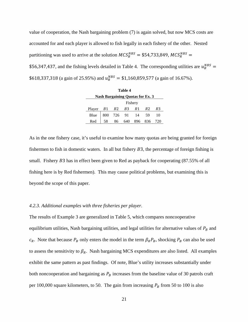
$56,347,437, and the fishing levels detailed in Table 4. The corresponding utilities are 𝑢𝑢𝐵𝐵𝑁𝑁𝐵𝐵𝑁𝑁 =
$618,337,318 (a gain of 25.95%) and 𝑢𝑢𝑅𝑅𝑁𝑁𝐵𝐵𝑁𝑁 = $1,160,859,577 (a gain of 16.67%).
Table 4 Nash Bargaining Quotas for Ex. 3
Fishery Player 𝐵𝐵1 𝐵𝐵2 𝐵𝐵3 𝑅𝑅1 𝑅𝑅2 𝑅𝑅3 Blue 800 726 91 14 59 10 Red 58 86 640 896 836 720
As in the one fishery case, it’s useful to examine how many quotas are being granted for foreign
fishermen to fish in domestic waters. In all but fishery 𝐵𝐵3, the percentage of foreign fishing is
small. Fishery 𝐵𝐵3 has in effect been given to Red as payback for cooperating (87.55% of all
fishing here is by Red fishermen). This may cause political problems, but examining this is
beyond the scope of this paper.
4.2.3. Additional examples with three fisheries per player.
The results of Example 3 are generalized in Table 5, which compares noncooperative
equilibrium utilities, Nash bargaining utilities, and legal utilities for alternative values of 𝑃𝑃𝐵𝐵 and
𝑐𝑐𝑅𝑅. Note that because 𝑃𝑃𝐵𝐵 only enters the model in the term 𝛽𝛽𝑅𝑅𝑃𝑃𝐵𝐵, shocking 𝑃𝑃𝐵𝐵 can also be used
to assess the sensitivity to 𝛽𝛽𝑅𝑅. Nash bargaining MCS expenditures are also listed. All examples
exhibit the same pattern as past findings. Of note, Blue’s utility increases substantially under
both noncooperation and bargaining as 𝑃𝑃𝐵𝐵 increases from the baseline value of 30 patrols craft
per 100,000 square kilometers, to 50. The gain from increasing 𝑃𝑃𝐵𝐵 from 50 to 100 is also

22
significant. Of course, viewing this decision in isolation neglects the possibility Red may
respond by investing in more maritime militias, offsetting the increase in Blue patrols. The
strategic interaction between investments in patrols and maritime militias is left as a point of
future research.
Table 5 Utilities for Additional Examples with Multiple Fisheries
𝑢𝑢𝐵𝐵𝑁𝑁𝑁𝑁 𝑢𝑢𝐵𝐵𝑁𝑁𝐵𝐵𝑁𝑁 𝑢𝑢𝐵𝐵𝑘𝑘𝑙𝑙𝑙𝑙𝑎𝑎𝑘𝑘 𝑢𝑢𝑅𝑅𝑁𝑁𝑁𝑁 𝑢𝑢𝑅𝑅𝑁𝑁𝐵𝐵𝑁𝑁 𝑢𝑢𝑅𝑅
𝑘𝑘𝑙𝑙𝑙𝑙𝑎𝑎𝑘𝑘 𝑀𝑀𝑀𝑀𝑆𝑆𝐵𝐵𝑁𝑁𝐵𝐵𝑁𝑁 𝑀𝑀𝑀𝑀𝑆𝑆𝑅𝑅𝑁𝑁𝐵𝐵𝑁𝑁
Parameters billions of USD millions of USD
Baseline (Ex. 3) .49 .62 .7700 .99 1.16 .9641 54.73 56.35 𝑃𝑃𝐵𝐵 = 50 .59 .67 .7715 .97 1.07 .9641 46.53 48.25 𝑃𝑃𝐵𝐵 = 100 .63 .71 .7748 .91 1.02 .9641 34.12 60.63
𝑐𝑐𝑅𝑅 = $150,000 .58 .69 .7700 .86 .98 .8887 44.08 52.17 𝑐𝑐𝑅𝑅 = $200,000 .71 .76 .7700 .72 .77 .7704 50.77 51.36
5. Conclusion and Future Work
This paper modeled a scenario akin to the ECS, where two maritime nations in close proximity
faced the decisions of how many legal fishing quotas to issue and how much to invest in MCS.
Consistent with observed behavior in the ECS, the model predicts illegal encroachments on
account of excessive issuance of quotas. Also consistent with observed behavior, each state
underinvests in MCS. The paper thus provides a rational explanation for illegal encroachments
and substandard MCS beyond the typical explanations of uncontrollable criminal activity and a
lack of political will to implement strong MCS. A bargaining problem was also solved which
quantified the substantial gains to be had from cooperation. In the bargain, the player with lower
costs, either by virtue of lower opportunity costs or more patrols and maritime militias, is seen to
achieve more than the optimal utility he could achieve in the absence of a nearby player. This
gain is realized through legal quotas for the low-cost player in the high-cost player’s waters.

23
The Gordon-Schaeffer fisheries model with logistics growth and a constant-effort harvesting
rates was used throughout this paper. Future research ought to perform similar analysis with
alternative fisheries models. Additional complicating factors should also to be assessed, such as
migration of species, discounted payoffs, and stochastic growth and harvest rates. Problems with
many more than three fisheries, and more than two players, are perhaps the most critical point of
future research as such a scenario is required to truly model the ECS, and thus use the model for
policy recommendations. All of these model extensions will require sophisticated computational
techniques.
A few other lines of future work are pertinent. As mentioned in Section 2, an empirical analysis
of the effectiveness of maritime militias is lacking in the literature. Such a study would improve
the analysis presented here by giving evidence-based assessments of 𝛽𝛽𝐵𝐵 and 𝛽𝛽𝑅𝑅. Accounting for
illegal third-parties, such as long-distance fishermen entering the ECS and unloading their catch
at far-off ports would also add realism to the model. Lastly, congested maritime environments
where there is not a legal delineation of fishing rights is an important area of study. Such is the
situation in the SCS, for example, where the consequences of opposing nations’ patrol craft
confronting one another becomes an important consideration that wasn’t relevant in this paper.
Not only do interacting patrols likely reduce the deterrent effect of patrols (as fishermen can
sound a distress call if confronted by opposition patrols), but the threat of escalation to greater
conflict may increase.

24
Appendix A. Proofs of Theorems 1 - 3. This appendix restates and proves Theorems 1, 2, and 3. Throughout, notation is used that
assumed each player owns only one fishery. To support the proofs, a useful, nonrestrictive
assumption is stated.
Assumption 1. Based on the statistical improbability of the contrary, it’s assumed open access
levels (the levels of biomasses at which rents are 0) are never exactly identical for Blue and Red
fishermen. That is, 𝑐𝑐𝐵𝐵𝑝𝑝𝐵𝐵𝑞𝑞𝐵𝐵
≠ 𝑐𝑐𝑅𝑅+𝛽𝛽𝑅𝑅𝑃𝑃𝐵𝐵𝐵𝐵𝑝𝑝𝐵𝐵𝑞𝑞𝐵𝐵
and 𝑐𝑐𝐵𝐵+𝛽𝛽𝐵𝐵𝑃𝑃𝐵𝐵𝑅𝑅𝑝𝑝𝑅𝑅𝑞𝑞𝑅𝑅
≠ 𝑐𝑐𝑅𝑅𝑝𝑝𝑅𝑅𝑞𝑞𝑅𝑅
.
A.1. Proof of Theorem 1
Theorem 1. Existence of a unique subgame equilibrium.
When Blue and Red each own only one fishery, any instantiation of the game’s parameters and
choice of the overall game’s decision variables yields a unique subgame equilibrium (SGE).
Proof.
It’s first be proved that for any instantiation, a SGE exists. Consider the following algorithm
which takes the parameters and (𝐹𝐹𝐵𝐵,𝐹𝐹𝑅𝑅) as given, and seeks values of the SGVs:
Algorithm A1. Finding a SGE.
1. Initiate 𝐹𝐹𝐵𝐵,𝐵𝐵 = 𝐹𝐹𝑅𝑅,𝐵𝐵 = 𝐹𝐹𝐵𝐵,𝑅𝑅 = 𝐹𝐹𝑅𝑅,𝑅𝑅 = 0.
2. Determine the set of SGVs, 𝐹𝐹′, to increase in the next iteration of the algorithm, as
follows. Define the maximum achievable rent as:
𝜋𝜋′ = max
⎩⎨
⎧𝜋𝜋𝐵𝐵,𝐵𝐵,𝜋𝜋𝑅𝑅,𝐵𝐵, 0; if 𝐹𝐹𝐵𝐵,𝑅𝑅 + 𝐹𝐹𝑅𝑅,𝑅𝑅 = 𝐹𝐹𝑅𝑅 ,𝐹𝐹𝐵𝐵,𝐵𝐵 + 𝐹𝐹𝑅𝑅,𝐵𝐵 < 𝐹𝐹𝐵𝐵𝜋𝜋𝐵𝐵,𝑅𝑅 ,𝜋𝜋𝑅𝑅,𝑅𝑅 , 0; if 𝐹𝐹𝐵𝐵,𝑅𝑅 + 𝐹𝐹𝑅𝑅,𝑅𝑅 < 𝐹𝐹𝑅𝑅 ,𝐹𝐹𝐵𝐵,𝐵𝐵 + 𝐹𝐹𝑅𝑅,𝐵𝐵 = 𝐹𝐹𝐵𝐵
0; if 𝐹𝐹𝐵𝐵,𝑅𝑅 + 𝐹𝐹𝑅𝑅,𝑅𝑅 = 𝐹𝐹𝑅𝑅 ,𝐹𝐹𝐵𝐵,𝐵𝐵 + 𝐹𝐹𝑅𝑅,𝐵𝐵 = 𝐹𝐹𝐵𝐵𝜋𝜋𝐵𝐵,𝐵𝐵,𝜋𝜋𝑅𝑅,𝐵𝐵,𝜋𝜋𝐵𝐵,𝑅𝑅 ,𝜋𝜋𝑅𝑅,𝑅𝑅 , 0; otherwise
.

25
If 𝜋𝜋′ = 0, stop. Otherwise, include all SGVs in 𝐹𝐹′ whose corresponding rent equals 𝜋𝜋′, and
can be increased without decreasing another SGV; that is, only 𝐹𝐹𝐵𝐵,𝐵𝐵 and 𝐹𝐹𝑅𝑅,𝐵𝐵 may only be in
𝐹𝐹′ if 𝐹𝐹𝐵𝐵,𝐵𝐵 + 𝐹𝐹𝑅𝑅,𝐵𝐵 < 𝐹𝐹𝐵𝐵 and 𝐹𝐹𝐵𝐵,𝑅𝑅 + 𝐹𝐹𝑅𝑅,𝑅𝑅 = 𝐹𝐹𝑅𝑅, and similarly for 𝐹𝐹𝐵𝐵,𝑅𝑅 and 𝐹𝐹𝑅𝑅,𝑅𝑅.
Before describing steps 3 through 6, note the following properties are maintained throughout
the algorithm:
Algorithm A1, Property 1. SGVs are never allowed to go below 0, and ∑ 𝐹𝐹𝑖𝑖,𝑘𝑘𝑖𝑖 ≤ 𝐹𝐹𝑘𝑘
remains true for both 𝑘𝑘 ∈ {𝐵𝐵,𝑅𝑅}.
Algorithm A1, Property 2. If 𝐹𝐹𝑖𝑖,𝑘𝑘 > 0, then 𝜋𝜋𝑖𝑖,𝑘𝑘 ≥ 0 and 𝜋𝜋𝑖𝑖,𝑘𝑘 ≥ 𝜋𝜋𝑖𝑖′,𝑘𝑘 for 𝑖𝑖′ ≠ 𝑖𝑖.
These two properties ensure all subgame constraints are satisfied throughout the algorithm,
other than those stating no profitable quotas are left unused. The latter condition is the
stopping condition for the algorithm (𝜋𝜋′ = 0).
3. Increase all SGVs in 𝐹𝐹′ while obeying the following rules:
i. Increase SGVs in 𝐹𝐹′ at rates such that their rents remain equal.
ii. Consider the case where, WLOG, 𝐹𝐹𝐵𝐵,𝑅𝑅 + 𝐹𝐹𝑅𝑅,𝑅𝑅 = 𝐹𝐹𝑅𝑅 (so that by definition 𝐹𝐹𝐵𝐵,𝑅𝑅 and 𝐹𝐹𝑅𝑅,𝑅𝑅
are not in 𝐹𝐹′). Modify 𝐹𝐹𝐵𝐵,𝑅𝑅 and 𝐹𝐹𝑅𝑅,𝑅𝑅 at rates such that 𝐹𝐹𝐵𝐵,𝑅𝑅 + 𝐹𝐹𝑅𝑅,𝑅𝑅 = 𝐹𝐹𝑅𝑅 remains true,
𝐹𝐹𝐵𝐵,𝑅𝑅 > 0 iff 𝜋𝜋𝐵𝐵,𝑅𝑅 ≥ 𝜋𝜋𝑅𝑅,𝑅𝑅, and 𝐹𝐹𝑅𝑅,𝑅𝑅 > 0 iff 𝜋𝜋𝐵𝐵,𝑅𝑅 ≤ 𝜋𝜋𝑅𝑅,𝑅𝑅.
iii. Return to step 2 whenever a new SGV enters 𝐹𝐹′, or when ∑ 𝐹𝐹𝑖𝑖′,𝑘𝑘𝑖𝑖′ = 𝐹𝐹𝑘𝑘 for any SGVs
in 𝐹𝐹′, or when the rent of a SGV in 𝐹𝐹′ becomes 0.

26
The proof this algorithm always produces a SGE is clear, after noting one additional property to
accompany Properties 1 and 2.
Algorithm A1, Property 3. 𝜋𝜋′ is either constant or decreasing linearly throughout the
algorithm. The former case occurs only when a SGV in 𝐹𝐹′ is increasing with a perfectly
offsetting decreasing in a SGV not in 𝐹𝐹′, a process which eventually stops when the
decreasing SGV reaches 0, and is followed by a state where the only SGVs being modified
are increasing. Thus, every state where 𝜋𝜋′ is constant is followed by a state where it’s
linearly decreasing, and thus 𝜋𝜋′ will eventually reach 0.
𝜋𝜋′ = 0 implies either all quotas are exhausted, or neither player can achieve positive rent with
their remaining quotas. Thus, properties 1 through 3 imply the algorithm will terminate at a
subgame equilibrium.
To complete the proof of Theorem 1, it’s now shown whenever a SGE exists, it must be unique.
This is shown in two parts: first, if there exists a SGE resulting in biomasses 𝑥𝑥𝐵𝐵𝑁𝑁𝑆𝑆𝑆𝑆 and 𝑥𝑥𝑅𝑅𝑁𝑁𝑆𝑆𝑆𝑆 , it’s
shown any SGE must yield these biomasses; next, it’s shown biomasses at SGE are sufficient to
uniquely determine the values of the SGVs.
Assume Algorithm A1 was used to produce a SGE with biomasses 𝑥𝑥𝐵𝐵𝑁𝑁𝑆𝑆𝑆𝑆 and 𝑥𝑥𝑅𝑅𝑁𝑁𝑆𝑆𝑆𝑆 . Now
consider an alternative SGE; its biomasses and SGVs will be referenced using the “prime”
superscript (′) to differentiate between the original SGE, superscripted by 𝑆𝑆𝑆𝑆𝑆𝑆. Assume one of
the biomasses has increased; WLOG, 𝑥𝑥𝐵𝐵′ > 𝑥𝑥𝐵𝐵𝑁𝑁𝑆𝑆𝑆𝑆 . This means at least one player, WLOG Blue,
was previously fishing in Blue waters and is now fishing less in Blue waters: 0 ≤ 𝐹𝐹𝐵𝐵,𝐵𝐵′ < 𝐹𝐹𝐵𝐵,𝐵𝐵
𝑁𝑁𝑆𝑆𝑆𝑆 .
27
If Blue fishermen are not fishing in Red waters under the new SGE (𝐹𝐹𝑅𝑅,𝐵𝐵′ = 0), then they’re
using all available quotas in Blue waters: 𝐹𝐹𝐵𝐵,𝐵𝐵′ = 𝐹𝐹𝐵𝐵; otherwise constraints (6c) in the subgame
would be violated stating Blue doesn’t leave profitable quotas unused. This contradicts 𝐹𝐹𝐵𝐵,𝐵𝐵′ <
𝐹𝐹𝐵𝐵,𝐵𝐵𝑁𝑁𝑆𝑆𝑆𝑆 ≤ 𝐹𝐹𝐵𝐵, so assume instead Blue fishermen are fishing in Red waters. 𝐹𝐹𝑅𝑅,𝐵𝐵
′ > 0 implies 𝑥𝑥𝑅𝑅
has also increased, since by (6c) 𝑝𝑝𝐵𝐵𝑞𝑞𝐵𝐵𝑥𝑥𝐵𝐵𝑁𝑁𝑆𝑆𝑆𝑆 ≥ 𝑝𝑝𝑅𝑅𝑞𝑞𝑅𝑅𝑥𝑥𝑅𝑅𝑁𝑁𝑆𝑆𝑆𝑆 − 𝛽𝛽𝐵𝐵𝑃𝑃𝑅𝑅 → 𝑝𝑝𝐵𝐵𝑞𝑞𝐵𝐵𝑥𝑥𝐵𝐵′ > 𝑝𝑝𝑅𝑅𝑞𝑞𝑅𝑅𝑥𝑥𝑅𝑅𝑁𝑁𝑆𝑆𝑆𝑆 −
𝛽𝛽𝐵𝐵𝑃𝑃𝑅𝑅 and 𝑝𝑝𝐵𝐵𝑞𝑞𝐵𝐵𝑥𝑥𝐵𝐵′ ≤ 𝑝𝑝𝑅𝑅𝑞𝑞𝑅𝑅𝑥𝑥𝑅𝑅′ − 𝛽𝛽𝐵𝐵𝑃𝑃𝑅𝑅 → 𝑥𝑥𝑅𝑅𝑁𝑁𝑆𝑆𝑆𝑆 < 𝑥𝑥𝑅𝑅′ . Since both biomasses have increased, at
least one player’s fishermen are using less overall quotas, hence they have quotas to use which
are profitable at these higher levels of biomass (otherwise, the original SGE would violate (6c)),
thus (6d) is violated and this is not a SGE. In sum, there can be no SGE with 𝑥𝑥𝐵𝐵 > 𝑥𝑥𝐵𝐵𝑁𝑁𝑆𝑆𝑆𝑆, and by
analogy none with 𝑥𝑥𝑅𝑅 > 𝑥𝑥𝑅𝑅𝑁𝑁𝑆𝑆𝑆𝑆 .
Assume instead one of the biomasses has declined; WLOG, 𝑥𝑥𝐵𝐵′ < 𝑥𝑥𝐵𝐵𝑁𝑁𝑆𝑆𝑆𝑆 . At least one of the
players, WLOG Blue, must be using more quotas in Blue waters: 𝐹𝐹𝐵𝐵,𝐵𝐵′ > 𝐹𝐹𝐵𝐵,𝐵𝐵
𝑁𝑁𝑆𝑆𝑆𝑆 ≥ 0. She would
have used this larger amount of quotas in Blue waters under the original SGE so as not to violate
(6e), unless 𝐹𝐹𝑅𝑅,𝐵𝐵𝑁𝑁𝑆𝑆𝑆𝑆 > 0 and Blue fishermen were earning greater or equal rent compared to Blue
waters. This implies 𝑥𝑥𝑅𝑅′ < 𝑥𝑥𝑅𝑅𝑁𝑁𝑆𝑆𝑆𝑆 , as otherwise Blue would now be receiving strictly greater rent
in Red waters, entailing 𝐹𝐹𝐵𝐵,𝐵𝐵′ = 0. Because both biomasses have declined, at least one player’s
fishermen are using more overall quotas, implying in the original SGE they had additional quotas
to use which were profitable at higher biomasses (if not, (6c) would be violated in the new SGE),
hence (6d) was violated by the original SGE, a contradiction. In sum, under any SGE, Blue
biomass must be 𝑥𝑥𝐵𝐵𝑁𝑁𝑆𝑆𝑆𝑆 , and by analogy Red must be 𝑥𝑥𝑅𝑅𝑁𝑁𝑆𝑆𝑆𝑆 .

28
Knowing any SGE must have the same levels of biomass, the proof SGEs are unique is
concluded by showing biomasses can uniquely determine the values of the SGVs. First note
biomasses can immediately identify which SGVs must be 0. For example, if Red biomass is less
than 𝑐𝑐𝐵𝐵+𝛽𝛽𝐵𝐵𝑃𝑃𝑅𝑅𝑝𝑝𝑅𝑅𝑞𝑞𝑅𝑅
(Blue’s so-called open access level in Red waters), then 𝐹𝐹𝑅𝑅,𝐵𝐵 = 0; similar
statements hold for 𝐹𝐹𝐵𝐵,𝐵𝐵, 𝐹𝐹𝐵𝐵,𝑅𝑅, and 𝐹𝐹𝑅𝑅,𝑅𝑅. If 𝑥𝑥𝐵𝐵𝑁𝑁𝑆𝑆𝑆𝑆 > 𝑥𝑥𝑅𝑅𝑁𝑁𝑆𝑆𝑆𝑆 −𝛽𝛽𝐵𝐵𝑃𝑃𝑅𝑅𝑝𝑝𝑅𝑅𝑞𝑞𝑅𝑅
, then Blue fishermen earn
greater rent in Blue water and 𝐹𝐹𝑅𝑅,𝐵𝐵 = 0; similar statements hold for 𝐹𝐹𝐵𝐵,𝐵𝐵, 𝐹𝐹𝐵𝐵,𝑅𝑅, and 𝐹𝐹𝑅𝑅,𝑅𝑅. Now
consider three possibilities: only one SGV is potentially nonzero; only two are potentially
nonzero; and three are potentially nonzero. Note four nonzero SGVs is impossible, as either
𝑥𝑥𝐵𝐵𝑁𝑁𝑆𝑆𝑆𝑆 > 𝑥𝑥𝑅𝑅𝑁𝑁𝑆𝑆𝑆𝑆 −𝛽𝛽𝐵𝐵𝑃𝑃𝑅𝑅𝑝𝑝𝑅𝑅𝑞𝑞𝑅𝑅
, implying 𝐹𝐹𝑅𝑅,𝐵𝐵 = 0, or 𝑥𝑥𝐵𝐵𝑁𝑁𝑆𝑆𝑆𝑆 < 𝑥𝑥𝑅𝑅𝑁𝑁𝑆𝑆𝑆𝑆 −𝛽𝛽𝐵𝐵𝑃𝑃𝑅𝑅𝑝𝑝𝑅𝑅𝑞𝑞𝑅𝑅
, implying 𝐹𝐹𝐵𝐵,𝐵𝐵 = 0, or 𝑥𝑥𝐵𝐵𝑁𝑁𝑆𝑆𝑆𝑆 =
𝑥𝑥𝑅𝑅𝑁𝑁𝑆𝑆𝑆𝑆 −𝛽𝛽𝐵𝐵𝑃𝑃𝑅𝑅𝑝𝑝𝑅𝑅𝑞𝑞𝑅𝑅
, implying 𝑥𝑥𝐵𝐵𝑁𝑁𝑆𝑆𝑆𝑆 −𝛽𝛽𝑅𝑅𝑃𝑃𝐵𝐵𝑝𝑝𝐵𝐵𝑞𝑞𝐵𝐵
< 𝑥𝑥𝑅𝑅𝑁𝑁𝑆𝑆𝑆𝑆 and 𝐹𝐹𝐵𝐵,𝑅𝑅 = 0.
If only one SGV may be nonzero, assume WLOG this is 𝐹𝐹𝐵𝐵,𝐵𝐵. It’s apparent this has a unique
value; simply increase 𝐹𝐹𝐵𝐵,𝐵𝐵 until 𝑥𝑥𝐵𝐵 = 𝑥𝑥𝐵𝐵𝑁𝑁𝑆𝑆𝑆𝑆 . If two nonzero SGVs are possible there are three
general cases. First, assume one player may be fishing in one fishery, and the other player in the
other; WLOG, 𝐹𝐹𝐵𝐵,𝐵𝐵 and 𝐹𝐹𝑅𝑅,𝑅𝑅 may be nonzero. As when only one SGV could be nonzero, the
unique SGE is clear: increase 𝐹𝐹𝐵𝐵,𝐵𝐵 until 𝑥𝑥𝐵𝐵 = 𝑥𝑥𝐵𝐵𝑁𝑁𝑆𝑆𝑆𝑆 , and do likewise for 𝐹𝐹𝑅𝑅,𝑅𝑅. If instead one
player is fishing in both waters, assume WLOG 𝐹𝐹𝐵𝐵,𝐵𝐵 and 𝐹𝐹𝑅𝑅,𝐵𝐵 may be nonzero. Again, the
unique solution mandates 𝐹𝐹𝐵𝐵,𝐵𝐵 and 𝐹𝐹𝑅𝑅,𝐵𝐵 are increased until stocks are depleted to 𝑥𝑥𝐵𝐵𝑁𝑁𝑆𝑆𝑆𝑆 and 𝑥𝑥𝑅𝑅𝑁𝑁𝑆𝑆𝑆𝑆 .
Lastly, assume both players may be fishing in one fishery; WLOG, 𝐹𝐹𝐵𝐵,𝐵𝐵 and 𝐹𝐹𝐵𝐵,𝑅𝑅 may be
nonzero. It’s known 𝑥𝑥𝐵𝐵𝑁𝑁𝑆𝑆𝑆𝑆 ≥𝑐𝑐𝐵𝐵
𝑝𝑝𝐵𝐵𝑞𝑞𝐵𝐵 and 𝑥𝑥𝐵𝐵𝑁𝑁𝑆𝑆𝑆𝑆 ≥
𝑐𝑐𝑅𝑅+𝛽𝛽𝑅𝑅𝑃𝑃𝐵𝐵𝐵𝐵𝑝𝑝𝐵𝐵𝑞𝑞𝐵𝐵
, and by Assumption 1 one of these
inequalities must be strict; WLOG, assume 𝑥𝑥𝐵𝐵𝑁𝑁𝑆𝑆𝑆𝑆 > 𝑐𝑐𝑅𝑅+𝛽𝛽𝑅𝑅𝑃𝑃𝐵𝐵𝐵𝐵𝑝𝑝𝐵𝐵𝑞𝑞𝐵𝐵
. By subgame constraint (6d), Red

29
fishermen must use all quotas, 𝐹𝐹𝐵𝐵,𝑅𝑅 = 𝐹𝐹𝑅𝑅. To uniquely determine 𝐹𝐹𝐵𝐵,𝐵𝐵, simply increase it until
𝑥𝑥𝐵𝐵 = 𝑥𝑥𝐵𝐵𝑁𝑁𝑆𝑆𝑆𝑆 . The final case assumes three SGVs may be nonzero; WLOG, 𝐹𝐹𝐵𝐵,𝐵𝐵, 𝐹𝐹𝐵𝐵,𝐵𝐵, and 𝐹𝐹𝑅𝑅,𝑅𝑅.
𝐹𝐹𝑅𝑅,𝑅𝑅 must be that which depletes Red biomass to 𝑥𝑥𝑅𝑅𝑁𝑁𝑆𝑆𝑆𝑆 . From here, the same logic can be applied
as when only 𝐹𝐹𝐵𝐵,𝐵𝐵 and 𝐹𝐹𝐵𝐵,𝑅𝑅 were allowed to be nonzero to determine their unique values; the one
amendment is that 𝐹𝐹𝐵𝐵,𝑅𝑅 = 𝐹𝐹𝑅𝑅 − 𝐹𝐹𝑅𝑅,𝑅𝑅, rather than 𝐹𝐹𝐵𝐵,𝑅𝑅 = 𝐹𝐹𝑅𝑅. In sum, knowing the biomasses at
the subgame equilibrium allows the SGVs to be uniquely determined.
To summarize the proof of Theorem 1: (i) by Algorithm A1 and the associated proof, a SGE
always exists; (ii) if there exists a SGE resulting in biomasses 𝑥𝑥𝐵𝐵𝑁𝑁𝑆𝑆𝑆𝑆 and 𝑥𝑥𝑅𝑅𝑁𝑁𝑆𝑆𝑆𝑆 , then any SGE
must result in these biomasses; (iii) SGE biomasses are sufficient to uniquely determine the
SGVs, and hence a unique SGE always exists.
A.2. Proof of Theorem 2
Theorem 2. Formulae for the unique subgame equilibrium via a partitioning of the
parameter and decision space.
Assume Blue and Red each own one fishery. The parameter and decision variable space can be
partitioned, such that in each region of the partition analytical formulae exist for the subgame
variables.
Proof.
The proof uses Theorem 1, as well as the notion that subgame equilibria can be categorized into
various “forms.” The form of a subgame equilibrium defines which SGVs are nonzero and
whether each player’s quotas are exhausted. For example, one form of a SGE could be
𝐹𝐹𝐵𝐵,𝐵𝐵,𝐹𝐹𝐵𝐵,𝑅𝑅 ,𝐹𝐹𝑅𝑅,𝑅𝑅 > 0, 𝐹𝐹𝑅𝑅,𝐵𝐵 = 0, 𝐹𝐹𝐵𝐵,𝐵𝐵 = 𝐹𝐹𝐵𝐵, and 𝐹𝐹𝐵𝐵,𝑅𝑅 + 𝐹𝐹𝑅𝑅,𝑅𝑅 = 𝐹𝐹𝑅𝑅. For each possible form, it’s

30
straightforward to derive necessary and sufficient conditions for the SGE to have that form, as is
deriving the analytical formulae for the SGVs. Continuing the example form just mentioned, the
formulae for the SGVs are derived by noting that since 𝐹𝐹𝐵𝐵,𝑅𝑅 ,𝐹𝐹𝑅𝑅,𝑅𝑅 > 0, Red’s rents must equate
(by (6c)): 𝑝𝑝𝐵𝐵𝑞𝑞𝐵𝐵𝑍𝑍𝐵𝐵 �1 − 𝑞𝑞𝐵𝐵𝑟𝑟𝐵𝐵�𝐹𝐹𝐵𝐵 + 𝐹𝐹𝐵𝐵,𝑅𝑅�� − 𝛽𝛽𝑅𝑅𝑃𝑃𝐵𝐵 − 𝛽𝛽𝑚𝑚𝑚𝑚𝑅𝑅 = 𝑝𝑝𝑅𝑅𝑞𝑞𝑅𝑅𝑍𝑍𝑅𝑅 �1 − 𝑞𝑞𝑅𝑅
𝑟𝑟𝑅𝑅𝐹𝐹𝑅𝑅,𝑅𝑅�. Combined
with 𝐹𝐹𝐵𝐵,𝑅𝑅 + 𝐹𝐹𝑅𝑅,𝑅𝑅 = 𝐹𝐹𝑅𝑅, this yields a linear system with two equations and two unknowns, which
has solution:
𝐹𝐹𝐵𝐵,𝑅𝑅 = −𝑟𝑟𝑅𝑅𝑝𝑝𝐵𝐵𝑞𝑞𝐵𝐵2𝑍𝑍𝐵𝐵𝐹𝐹𝐵𝐵+𝑟𝑟𝐵𝐵𝑝𝑝𝑅𝑅𝑞𝑞𝑅𝑅
2𝑍𝑍𝑅𝑅𝐹𝐹𝑅𝑅+𝑟𝑟𝑅𝑅𝑟𝑟𝐵𝐵[𝑝𝑝𝐵𝐵𝑞𝑞𝐵𝐵𝑍𝑍𝐵𝐵−𝑝𝑝𝑅𝑅𝑞𝑞𝑅𝑅𝑍𝑍𝑅𝑅−𝛽𝛽𝑅𝑅𝑃𝑃𝐵𝐵−𝛽𝛽𝑚𝑚𝑚𝑚𝑅𝑅]𝑟𝑟𝐵𝐵𝑝𝑝𝑅𝑅𝑞𝑞𝑅𝑅
2𝑍𝑍𝑅𝑅+𝑟𝑟𝑅𝑅𝑝𝑝𝐵𝐵𝑞𝑞𝐵𝐵2𝑍𝑍𝐵𝐵
(8)
𝐹𝐹𝑅𝑅,𝑅𝑅 = 𝑟𝑟𝑅𝑅𝑝𝑝𝐵𝐵𝑞𝑞𝐵𝐵2𝑍𝑍𝐵𝐵𝐹𝐹𝐵𝐵+𝑟𝑟𝑅𝑅𝑝𝑝𝐵𝐵𝑞𝑞𝐵𝐵
2𝑍𝑍𝐵𝐵𝐹𝐹𝑅𝑅−𝑟𝑟𝑅𝑅𝑟𝑟𝐵𝐵[𝑝𝑝𝐵𝐵𝑞𝑞𝐵𝐵𝑍𝑍𝐵𝐵−𝑝𝑝𝑅𝑅𝑞𝑞𝑅𝑅𝑍𝑍𝑅𝑅−𝛽𝛽𝑅𝑅𝑃𝑃𝐵𝐵−𝛽𝛽𝑚𝑚𝑚𝑚𝑅𝑅]𝑟𝑟𝑅𝑅𝑝𝑝𝐵𝐵𝑞𝑞𝐵𝐵
2𝑍𝑍𝐵𝐵+𝑟𝑟𝐵𝐵𝑝𝑝𝑅𝑅𝑞𝑞𝑅𝑅2𝑍𝑍𝑅𝑅
. (9)
𝐹𝐹𝐵𝐵,𝐵𝐵 = 𝐹𝐹𝐵𝐵 and 𝐹𝐹𝑅𝑅,𝐵𝐵 = 0 is given. Identifying necessary and sufficient conditions is a simple
matter of checking which of constraints (6c) and (6d) are applicable, and imposing strict
positivity constraints. In this example, those conditions are:
Positivity of 𝐹𝐹𝐵𝐵,𝑅𝑅: 0 < 𝐹𝐹𝐵𝐵,𝑅𝑅 (10)
Positivity of 𝐹𝐹𝑅𝑅,𝑅𝑅: 0 < 𝐹𝐹𝑅𝑅,𝑅𝑅 (11)
Blue fishermen achieve nonnegative rent in Blue waters: 𝜋𝜋𝐵𝐵,𝐵𝐵 ≥ 0 (12)
Red fishermen’s rents are nonnegative: 𝜋𝜋𝐵𝐵,𝑅𝑅 ≥ 0. (13)
By virtue of (8) and (9), constraints (10) – (13) are linear in 𝐹𝐹𝐵𝐵 and 𝐹𝐹𝑅𝑅. Also note (12) ensures
𝜋𝜋𝐵𝐵,𝐵𝐵 ≥ 𝜋𝜋𝑅𝑅,𝐵𝐵, since by construction 𝜋𝜋𝐵𝐵,𝑅𝑅 = 𝜋𝜋𝑅𝑅,𝑅𝑅 → 𝑝𝑝𝐵𝐵𝑞𝑞𝐵𝐵𝑥𝑥𝐵𝐵 − 𝛽𝛽𝑅𝑅𝑃𝑃𝐵𝐵 − 𝛽𝛽𝑚𝑚𝑚𝑚𝑅𝑅 = 𝑝𝑝𝑅𝑅𝑞𝑞𝑅𝑅𝑥𝑥𝑅𝑅 →
𝑝𝑝𝐵𝐵𝑞𝑞𝐵𝐵𝑥𝑥𝐵𝐵 > 𝑝𝑝𝑅𝑅𝑞𝑞𝑅𝑅𝑥𝑥𝑅𝑅 − 𝛽𝛽𝐵𝐵𝑃𝑃𝑅𝑅 − 𝛽𝛽𝑚𝑚𝑚𝑚𝐵𝐵 → 𝜋𝜋𝐵𝐵,𝐵𝐵 > 𝜋𝜋𝑅𝑅,𝐵𝐵. (13) ensures 𝜋𝜋𝑅𝑅,𝑅𝑅 ≥ 0, since 𝜋𝜋𝐵𝐵,𝑅𝑅 = 𝜋𝜋𝑅𝑅,𝑅𝑅.
This same procedure for finding the subgame equilibrium formula and necessary and sufficient

31
conditions can be done for all possibly forms (there are a total of 29), and is omitted for space.
With this notion in hand the proof of the theorem is as follows:
• For a subgame equilibrium of a particular form: (i) the SGVs must solve an associated
system of linear equations and unknowns with a unique solution; (ii) necessary and sufficient
conditions exist for the SGE to have that form.
• Given values of the parameters and decision variables, produce a SGE via Algorithm A1. By
Theorem 1, this is the unique SGE.
• The SGE will have some form. By the necessity of the conditions for each form, those
conditions must hold, and hence the 29 sets of conditions encompass the entire
parameter/decision space.
• If any other set of conditions held, then by sufficiency a SGE of another form would hold,
which is impossible because SGEs are unique.
• Therefore, for any instantiation of the parameters and decision variables the conditions of one
and only one form may hold. This completes the proof.
A.3. Proof of Theorem 3
Theorem 3
Assume Blue and Red each own one fishery. For a given strategy of the other player, responding
with 𝑚𝑚𝑘𝑘 > 0 can yield at most equivalent utility as using 𝑚𝑚𝑘𝑘 = 0. If costs of MCS are nonzero,
then 𝑚𝑚𝑘𝑘 > 0 yields strictly less utility than 𝑚𝑚𝑘𝑘 = 0.
Proof.
WLOG, assume Blue is using non-zero MCS: 𝑚𝑚𝐵𝐵 > 0. Unilaterally changing strategy to 𝑚𝑚𝐵𝐵 =
0 only affects the costs imposed on Blue fishermen in Blue waters. If 𝐹𝐹𝑅𝑅,𝐵𝐵 does not change at

32
subgame equilibrium on account of the change in 𝑚𝑚𝐵𝐵 (because if was not previously profitable to
illegally fish in Red waters, and is still not), then all SGVs are unchanged and Blue’s utility is
either the same (if MCS is costless) or has increased (if MCS costs money). If 𝐹𝐹𝑅𝑅,𝐵𝐵 does change,
then it increases due to the reduction in costs. This means either: (i) Blue extracts rent from Red
waters, improving her utility; or (ii) Blue fishermen have diverted from Blue to Red waters. In
the latter case, Blue can simply issue more quotas to replace those who diverted to Red waters,
establishing a subgame equilibrium equivalent to that when 𝑚𝑚𝐵𝐵 > 0, but with a higher value of
𝐹𝐹𝑅𝑅,𝐵𝐵. By the previous logic, Blue utility has increased. This completes the proof.
Appendix B. Algorithm to find intervals where optimal responses are non-piecewise.
This appendix provides an annotated algorithm to identify intervals in 𝐹𝐹𝐵𝐵-space where Red’s
optimal response is a non-piecewise function, and likewise for Blue’s optimal response in
intervals of 𝐹𝐹𝑅𝑅-space. The algorithm works by finding which conditions partitioning the
subgame equilibrium forms (see Appendix A.2) could be satisfied, given the model parameters,
and then identifies key intersections of the conditions.
Algorithm B1. Identifying the critical intervals of 𝑭𝑭𝑩𝑩 and 𝑭𝑭𝑹𝑹.
Given values of 𝑍𝑍𝐵𝐵, 𝑍𝑍𝑅𝑅, 𝑐𝑐𝐵𝐵, 𝑐𝑐𝑅𝑅, 𝛽𝛽𝐵𝐵, 𝛽𝛽𝑅𝑅, 𝑃𝑃𝐵𝐵𝐵𝐵, 𝑃𝑃𝐵𝐵𝑅𝑅, 𝑟𝑟𝐵𝐵, 𝑟𝑟𝑅𝑅, 𝑞𝑞𝐵𝐵, 𝑞𝑞𝑅𝑅, 𝑝𝑝𝐵𝐵, and 𝑝𝑝𝑅𝑅:
1. Eliminate infeasible SGE forms and redundant conditions, based on parameter values. For
example, if a condition states 𝑎𝑎 > 𝑏𝑏 yet parameters dictate 𝑎𝑎 < 𝑏𝑏, that form in infeasible.
Inconsistencies such as 𝐹𝐹𝑅𝑅 > 𝑎𝑎 and 𝐹𝐹𝑅𝑅 < 𝑏𝑏 also eliminates forms. Redundant conditions
within a form arise when 𝐹𝐹𝑅𝑅 > 𝑎𝑎 and 𝐹𝐹𝑅𝑅 > 𝑏𝑏 are both conditions.

33
2. Collect all remaining conditions and treat them as equalities. Identify where they intersect
and initialize lists of intersection points in 𝐹𝐹𝐵𝐵-space and 𝐹𝐹𝑅𝑅-space; call them B-list and R-list.
3. Between points in B-list, order the conditions by 𝐹𝐹𝑅𝑅-value as a function of 𝐹𝐹𝐵𝐵. Do the
same for R-list.
4. Between points in B-list, identify critical conditions which, once crossed as 𝐹𝐹𝑅𝑅 increases,
move the subgame equilibrium into a different form. Do the same for R-list.
5. Identify values in B-list where the sequences of critical conditions found in step 4 changes,
indicating the possibility the formula for the optimal Red response will change. Do the same
for values of R-list.
6. Between consecutive points in B-list, find constrained optimal responses, where Red’s
response is constrained to be between consecutive critical conditions. Add to B-list any
values where these constrained optimal responses become binding, hence eliminating any
piecewise constrained optimal responses. Do the same for R-list.
7. Between consecutive points in B-list, determine the unconstrained optimal response by
identifying the best constrained optimal response. Add additional values to B-list wherever
the best constrained optimal response between two points changes, thus eliminating any
piecewise unconstrained optima. Do the same for R-list.

34
References
Borsky, Stefan, and Paul A Raschky. 2011. “A Spatial Econometric Analysis of Compliance
with an International Environmental Agreement on Open Access Resources.” Working
Papers in Economics and Statistics.
Brown, Matthew, William B. Haskell, and Milind Tambe. 2014. “Addressing Scalability and
Robustness in Security Games with Multiple Boundedly Rational Adversaries.” In
Decision and Game Theory for Security, edited by Radha Poovendran and Walid Saad,
8840:23–42. Lecture Notes in Computer Science. Cham: Springer International
Publishing. https://doi.org/10.1007/978-3-319-12601-2_2.
China Power Team. 2020. “Are Maritime Law Enforcement Forces Destabilizing Asia?” China
Power, April 3, 2020. https://chinapower.csis.org/maritime-forces-destabilizing-asia/.
Clark, Colin Whitcomb. 2006. The Worldwide Crisis in Fisheries: Economic Models and Human
Behavior. Cambridge; New York: Cambridge University Press.
Erickson, Andrew S. 2018. “Numbers Matter: China’s Three ‘Navies’ Each Have the World’s
Most Ships.” National Interest 26.
Erickson, Andrew S., and Conor M. Kennedy. 2016. “China’s Maritime Militia.” CNA
Corporation 7: 1–28.
Fang, Fei, Peter Stone, and Milind Tambe. 2015. “When Security Games Go Green: Designing
Defender Strategies to Prevent Poaching and Illegal Fishing.” In Proceedings of the
Twenty-Fourth International Joint Conference on Artificial Intelligence, 2589–95.
Fischer, Ronald D., and Leonard J. Mirman. 1996. “The Compleat Fish Wars: Biological and
Dynamic Interactions.” Journal of Environmental Economics and Management 30 (1):
34–42. https://doi.org/10.1006/jeem.1996.0003.
35
Grønbæk, Lone, Marko Lindroos, Gordon R Munro, and Pedro Pintassilgo. 2020. Game Theory
and Fisheries Management: Theory and Applications. Cham: Springer.
https://public.ebookcentral.proquest.com/choice/publicfullrecord.aspx?p=6111258.
Hsiao, Amanda. 2020. “Opportunities for Fisheries Enforcement Cooperation in the South China
Sea.” Marine Policy 121: 103569. https://doi.org/10.1016/j.marpol.2019.103569.
King, Dennis M., and Jon G. Sutinen. 2010. “Rational Noncompliance and the Liquidation of
Northeast Groundfish Resources.” Marine Policy 34 (1): 7–21.
https://doi.org/10.1016/j.marpol.2009.04.023.
Kuperan, K., and Jon G. Sutinen. 1998. “Blue Water Crime: Deterrence, Legitimacy, and
Compliance in Fisheries.” Law & Society Review 32 (2): 309–38.
https://doi.org/10.2307/827765.
Long, Le Kim, and Ola Flaaten. 2011. “A Stackelberg Analysis of the Potential for Cooperation
in Straddling Stock Fisheries.” Marine Resource Economics 26 (2): 119–39.
https://doi.org/10.5950/0738-1360-26.2.119.
Mangin, Tracey, Christopher Costello, James Anderson, Ragnar Arnason, Matthew Elliott, Steve
D. Gaines, Ray Hilborn, Emily Peterson, and Rashid Sumaila. 2018. “Are Fishery
Management Upgrades Worth the Cost?” Edited by Athanassios C. Tsikliras. PLOS ONE
13 (9): e0204258. https://doi.org/10.1371/journal.pone.0204258.
Miller, Steve, and Bruno Nkuiya. 2016. “Coalition Formation in Fisheries with Potential Regime
Shift.” Journal of Environmental Economics and Management 79: 189–207.
Nielsen, Jesper Raakjær, and Christoph Mathiesen. 2003. “Important Factors Influencing Rule
Compliance in Fisheries Lessons from Denmark.” Marine Policy 27 (5): 409–16.

36
Park, Young-kil. 2020. “The Role of Fishing Disputes in China–South Korea Relations.” The
National Bureau of Asian Research (NBR). https://map.nbr.org/2020/04/the-role-of-
fishing-disputes-in-china-south-korea-relations/.
Perry, Michael M. 2020. “Cooperative Maritime Law Enforcement and Overfishing in the South
China Sea.” Center for International Maritime Security, April 6, 2020.
http://cimsec.org/cooperative-maritime-law-enforcement-and-overfishing-in-the-south-
china-sea/43227.
Petrossian, Gohar A. 2015. “Preventing Illegal, Unreported and Unregulated (IUU) Fishing: A
Situational Approach.” Biological Conservation 189: 39–48.
https://doi.org/10.1016/j.biocon.2014.09.005.
———. 2019. The Last Fish Swimming: The Global Crime of Illegal Fishing. Global Crime and
Justice. Santa Barbara, California: Praeger, an imprint of ABC-CLIO, LLC.
Pitcher, Tony, Daniela Kalikoski, and Ganapathiraju Pramod. 2006. “Evaluations of Compliance
with the FAO (UN) Code of Conduct for Responsible Fisheries.” Fisheries Centre
Research Reports, University of British Columbia 14 (2).
Powell, Michael J.D. 1998. “Direct Search Algorithms for Optimization Calculations.” Acta
Numerica, 287–336.
Rosenberg, David. 2005. “Managing the Resources of the China Seas: China’s Bilateral
Fisheries Agreements with Japan, South Korea, and Vietnam.” The Asia-Pacific Journal
3 (6).
Shi, Leyuan, and Sigurdur Ólafsson. 2000. “Nested Partitions Method for Global Optimization.”
Operations Research 48 (3): 390–407. https://doi.org/10.1287/opre.48.3.390.12436.

37
Yonhap News. 2020. “S. Korea, China Agree to Cut Fishing in EEZs,” November 6, 2020.
https://en.yna.co.kr/view/AEN20201106010700320.
Zhang, Hongzhou. 2016. “Chinese Fishermen in Disputed Waters: Not Quite a ‘People’s War.’”
Marine Policy 68: 65–73. https://doi.org/10.1016/j.marpol.2016.02.018.
Zhang, Hongzhou, and Sam Bateman. 2017. “Fishing Militia, the Securitization of Fishery and
the South China Sea Dispute.” Contemporary Southeast Asia 39 (2): 288–314.
https://doi.org/10.1355/cs39-2b.