OCS Study MMS-93-0051

ALASKA oes .REGION

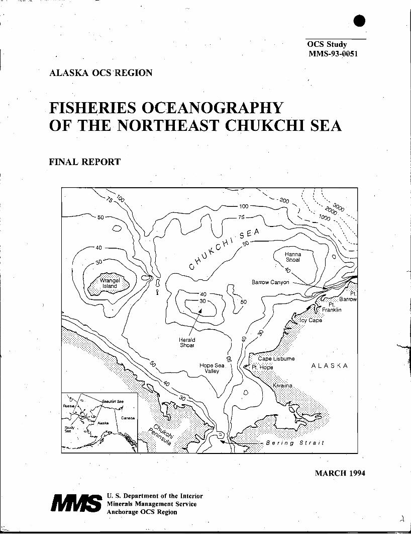
.FISHERIES OCEANOGRAPHY OF THE NORTHEAST CHUKCHI SEA

FINAL REPORT

, , ,,, I \ I

, ,

",, . , "'- .;:; .JOn....

voo"U , 7000 - " '-". -..... " ',', '. ",..

\ ,, ". ,

\ "-­'\.

."F't: .' -:.:- Barrow . ·-: pi .. ·

.... / :; Franklin

ALASKA

Strait

MARCH 1994

u. S. Department of the Interior Minerals Management Service Anchorage OCS Region

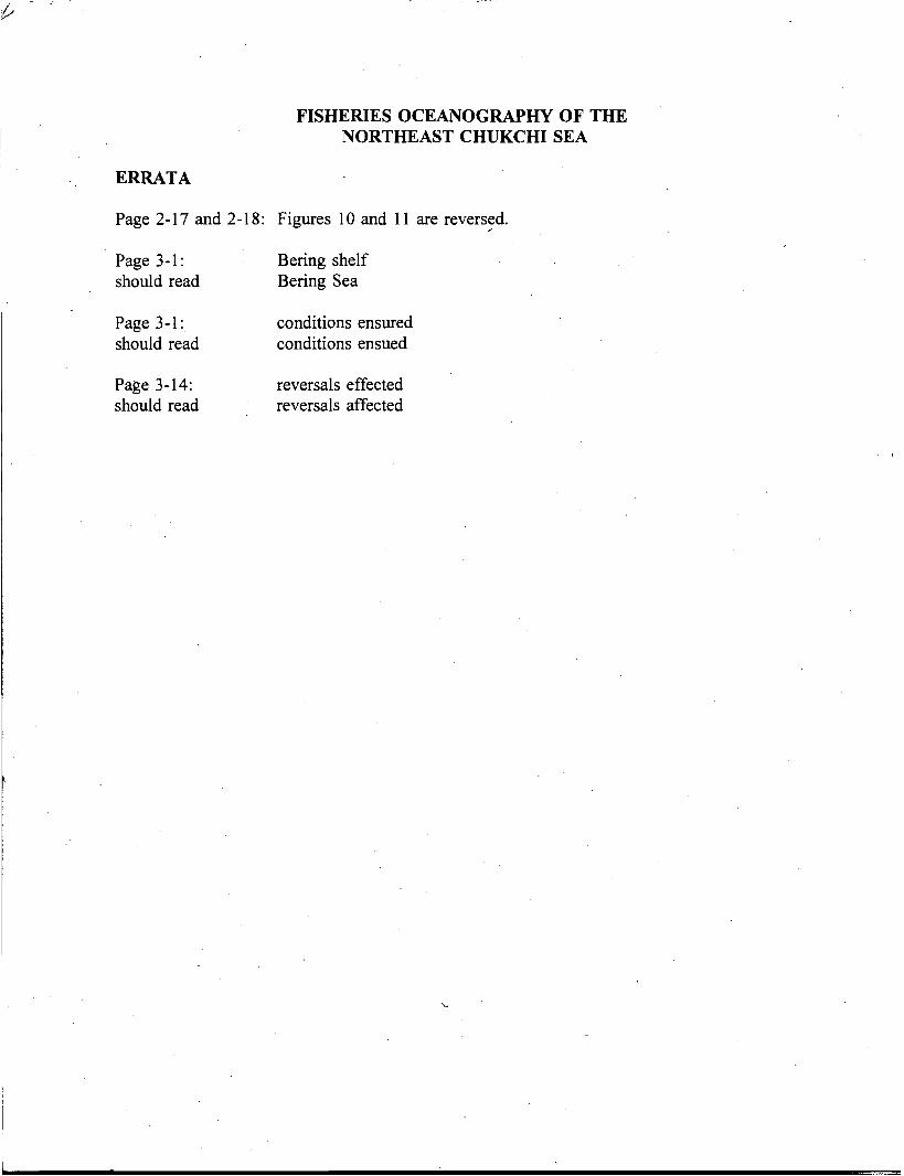
ERRATA

Page 2-17 and 2-18:

Page 3-1: should read

Page 3-1: should read

Page 3-14: should read

FISHERIES OCEANOGRAPHY OF THE NORTHEAST CHUKCHI SEA

Figures 10 and 11 are revers~d.

Bering shelf Bering Sea

conditions ensured conditions ensued

reversals effected reversals affected

OCS Study MMS-93-0051

FISHERIES OCEANOGRAPHY OF THE NORTHEAST CHUKCHI SEA

FINAL REPORT

Willard E. Barber Ronald L. Smith

School of Fisheries and Ocean Sciences

and

Thomas J. Weingartner Institute of Marine Sciences

University of Alaska Fairbanks Fairbanks, Alaska 99775

)

This study was funded by the . Alaska Outer Continental Shelf Region

of the Minerals Management Service U.S. Department of the Interior

Anchorage, Alaska

under Contract No. 14-35-0001-30559

March 1994

,,;

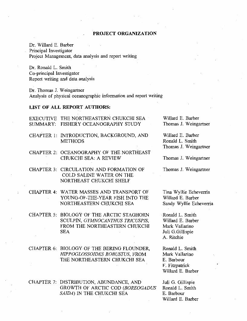
PROJECT ORGANIZATION

Dr. Willard E. Barber Principal Investigator Project Management, data analysis and report writing

Dr. Ronald L. Smith Co-principal Investigator Report writing and data analysis

Dr. Thomas 1. Weingartner Analysis of physical oceanographic information and report writing

LIST OF ALL REPORT AUTHORS:

EXECUTIVE SUMMARY:

THE NORTHEASTERN CHUKCHI SEA· FISHERY OCEANOGRAPHY STUDY

Willard E. Barber Thomas J. Weingartner

CHAPTER 1:

CHAPTER 2:

INTRODUCTION, BACKGROUND, AND METHODS

OCEANOGRAPHY OF THE NORTHEAST CHUKCHI SEA: A REVIEW

Willard E. Barber Ronald L. Smith Thomas J. Weingartner

Thomas J. Weingartner

CHAPTER 3: CIRCULATION AND FORMAnON OF COLD SALINE WATER ON THE

NORTHEAST CHUKCHI SHELF

Thomas 1. Weingartner

CHAPTER 4: WATER MASSES AND TRANSPORT OF YOUNG-OF-THE-YEAR FISH INTO THE NORTHEASTERN CHUKCHI SEA

Tina Wyllie Echeverria Willard E. Barber Sandy Wyllie Echeverria

CHAPTER 5: BIOLOGY OF THE ARCTIC STAGHORN SCULPIN, 'GYMNOCANTHUS TRICUSPIS, FROM THE NORTHEASTERN CHUKCHI SEA

.Ronald L. Smith Willard E. Barber Mark Vallarino Juli G.Gillispie A. Ritchie

CHAPTER 6: BIOLOGY OF THE BERING FLOUNDER, HIPPOGLOSSOIDES ROBUSTUS, FROM THE NORTHEASTERN CHUKCHI SEA

Ronald L. Smith Mark Vallarino E. Barbour F. Fitzpatrick Willard E. Barber

CHAPTER 7: .

DISTRIBUTION, ABUNDANCE, AND GROWTH OF ARCTIC COD (BOREOGADUS SAIDA) IN THE CHUKCHI SEA

Juli G. Gillispie Ronald L. Smith E. Barbour Willard E. Barber

CHAPTER 8: FOOD HABITS OF FOUR DEMERSAL CHUKCHI SEA FISHES

CHAPTER 9:' FISHES AND FISH ASSEMBLAGES OF THE NORTHEASTERN CHUKCHI SEA, ALASKA

CHAPTER 10: DISTRIBUTION OF MOLLUSKS IN THE NORTHEASTERN CHUKCHI SEA

CHAPTER 11: THE REPRODUCTIVE BIOLOGY AND . DISTRIBUTION OF SNOW CRAB FROM THE NORTHEASTERN CHUKCHI SEA

OTHER KEY PROJECT PERSONNEL:

Mark Vallarino and Chirk Chu Data management and analysis

\

Kenneth O. Coyle Juli G. Gillispie Ronald L. Smith Willard E. Barber

Willard E. Barber Mark Vallarino Ronald L. Smith

Howard M. Feder Nora R. Foster Stephen C. Jewett Thomas J. Weingartner Rae Baxter

J. M. Paul A. J. Paul Willard E. Barber

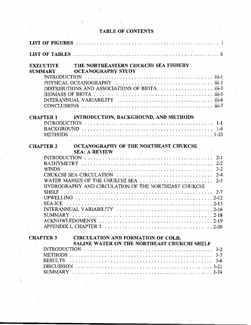
TABLE OF CONTENTS

LIST OF FIGURES

LIST OF TABLES ii

EXECUTIVE THE NORTHEASTERN CHUKCHI SEA FISHERY SUMMARY OCEANOGRAPHY STUDY

INTRODUCTION " iii-l PHYSICAL OCEANOGRAPHY .. " iii-l DISTRIBUTIONS AND ASSOCIATIONS OF BIOTA iii-3 BIOMASS OF BIOTA iii-5J • ••••••••••••••••••••••••••••••••

INTERANNUAL VARIABILITY iii-6 CONCLUSIONS iii-7

CHAPTER 1 INTRODUCTION, BACKGROUND, AND METHODS INTRODUCTION 1-1 BACKGROlJN"D '. . . . . . . . . . . . . . .. . . . . . ;.. . . . . . . . . . . . . . .. 1-4 METHODS ' 1-10

CHAPTER 2 OCEANOGRAPHY OF THE NORTHEAST CHUKCHI SEA: A REVIEW

BATHYMETRY - 2-2

HYDROGRAPHY AND CIRCULATION OF THE NORTHEAST CHUKCHI

INTRODUCTION 2-1

WINDS 2-2 ,CHUKCHI SEA CIRCULATION 2-4 WATER MASSES OF THE CHUKCHI SEA " 2-5

SHELF '.' _ 2-7 UPWELLING 2-12 SEA-ICE 2-13 INTERANNUAL VARIABILITY 2-16 SUMMARY 2-18 ACKNOWLEDGMENTS 2-19 APPENDIX I, CHAPTER 2 2-20

CHAPTER 3 CIRCULATION AND FORMATION OF COLD, SALINE WATER ON THE NORTHEAST CHUKCHI SHELF

INTRODUCTION 3-2 METHODS . . . . . . . . . . . . . . . . . . . . . . . . . . . . . . . . . . . . . . . . . . .. .. 3-3 RESULTS 3-6 DISCUSSION 3-21 SUMMARY 3-24

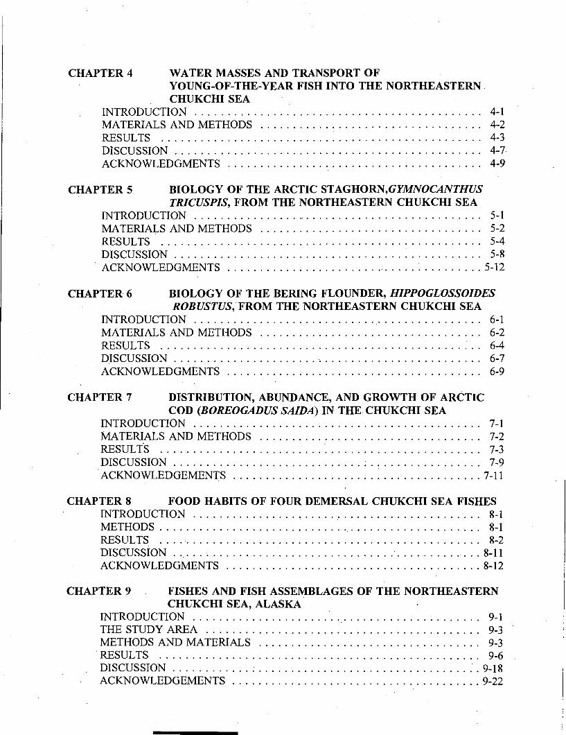
CHAPTER 4 WATER MASSES AND TRANSPORT OF YOUNG-OF-THE-YEAR FISH INTO THE NORTHEASTERN . CHUKCHI SEA

INTRODUCTION 4-1 MATERIALS AND METHODS 4-2 RESULTS .. . . . . . . . . .. 4-3 DISCUSSION .. . . . . . . . . . . . . . . . . . . . . . . . . . . . . . . . . . . . . . . . . . .. 4-7 ACKNOWLEDGMENTS 4-9

CHAPTER 5 BIOLOGY OF THE ARCTIC STAGHORN,GYMNOCANTHUS TRICUSPIS, FROM THE NORTHEASTERN CHUKCHI SEA

INTRODUCTION ,........................ 5-1 MATERIALS AND METHODS 5-2 RESULTS ;....................... 5-4 DISCUSSION . . . . . . . . . . . . . . . . . . . . . . . . . . . . . . . . . . . . . . . . . . . . . . .. 5-8

· ACKNOWLEDGMENTS 5-12

CHAPTER 6 BIOLOGY OF THE BERING FLOUNDER, HIPPOGLOSSOIDES ROBUSTUS,FROM THE NORTHEASTERN CHUKCHI SEA

INTRODUCTION " 6-1 MATERIALS AND METHODS 6-2 ·RESULTS .. . . . . . . . . . . . . . . . . . . . . . . . . . . . . . . ' ~ .. 6-4 DISCUSSION . . . . . . . . . . . . . . . . . . . . . . .. . . . . . . . . . . . . . . . . . . . . . . .. 6-7

· ACKNOWLEDGMENTS 6-9

CHAPTER 7 DISTRIBUTION, ABUNDANCE, AND GROWTH OF ARCTIC COD (BOREOGADUS SAIDA) IN THE CHUKCHI SEA

INTRODUCTION 7-1 MATERIALS AND METHODS 7-2 RESULT'S 7-3 DISCUSSION 7-9

.ACKNOWLEDGEMENTS 7-11

CHAPTER 8 FOOD HABITS OF FOUR DEMERSAL CHUKCHI SEA FISHES INTRODUCTION 8-1 METHODS '. . . . . . . . . . . . . . . . . . . .. 8-1 RESULTS 8-2 DISCUSSION ~ 8-11 ACKNOWLEDGMENTS 8-12

CHAPTER 9 FISHES AND FISH ASSEMBLAGES OF THE NORTHEASTERN CHUKCHI SEA, ALASKA

INTRODUCTION ~ " 9-1 THE STUDY AREA . . . . . . . . . . . . . . . . . . . . . . . . . . . . . . . . . . . . . . . . .. 9-3 METHODS AND MATERIALS 9-3

· RESULTS 9-6 DISCUSSION " .' . 9-18 ACKNOWLEDGEMENTS ; 9-22

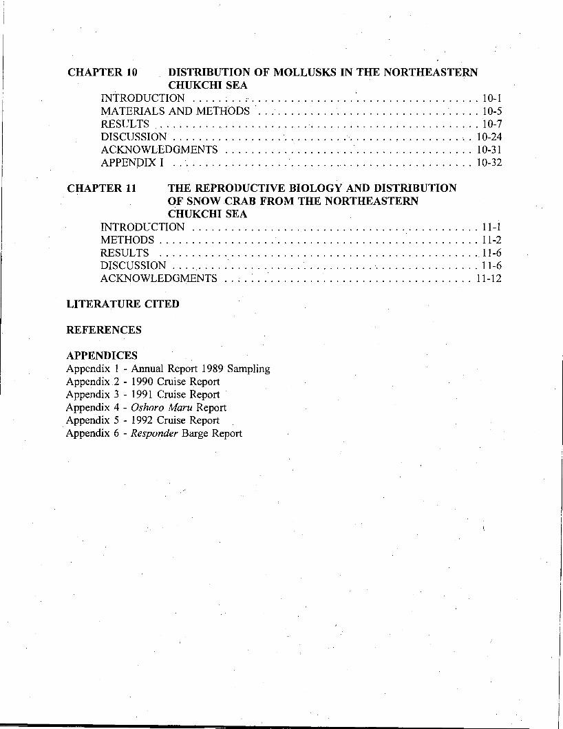
CHAPTER 10 DISTRIBUTION OF MOLLUSKS IN THE NORTHEASTERN CHUKCHI SEA

INTRODUCTION ~ .. ; ' 10-1 MATERIALS AND METHODS ' , 10-5 RESULTS, , ' ',' . 10-7 DISCUSSION , " . 10-24 ACKNOWLEDGMENTS 10-31 APPENDIX I " ' " , . . . . . . . . . . . . . . . . . . . 10-32

CHAPTER 11 THE REPRODUCTIVE BIOLOGY AND DISTRIBUTION OF SNOW CRAB FROM THE NORTHEASTERN CHUKCHI SEA

INTRODUCTION 11-1 METHODS ' 11-2 RESULTS ,11-6 DISCUSSION ',' " 11-6 ACKNOWLEDGMENTS 11-12

LITERATURE CITED

REFERENCES

APPENDICES Appendix 1 - Annual Report 1989 Sampling Appendix 2 - 1990 Cruise Report Appendix 3 - 1991 Cruise Report Appendix 4 - Oshoro Maru Report

,Appendix 5 - 1992 Cruise Report Appendix 6 - Responder Barge Report

\

LIST OF FIGURES

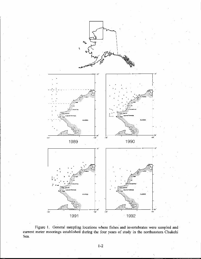
CHAPTER 1 Figure 1. General sampling locations where fishes and invertebrates were sampled and

current meter moorings established during the four years of study in the northeastern Chukchi Sea.

Figure 2a. Distribution of biomass (gC/m2) in· the northeastern Chukchi Sea, August-September 1986. The frontal zone (shown by the dashed line) presumably

. separates the mixed Bering Shelf/Anadyr Water in the west and north from the Alaska Coastal Water (FigUre 68 from Feder et al. 1989).

lFigure 2b. Carbon production estimates (gC/m2 yr- ) for the 37 stations occupied in the northeastern Chukchi Sea, August-September 1986.. The frontal zone (shown by

.. the dashed line) presumably separates the mixed Bering Shelf/Anadyr Water in the west and north from the Alaska Shelf/Anadyr Water in the west and north from the Alaska Coastal Water (Figure 69 from Feder et al. 1989)..

Figure 3. Distribution of macrofaunal coinmunities in the northeastern Chukchi Sea based on cluster and principal coordinate arialyses of abundance data collected August­September 1986 (Figure 69 from Feder et al. 1989).

. CHAPTER 2 Figure 1. Bathymetric and place names of the northern Bering and Chukchi Seas.

Figure 2. Temperature-salinity diagram of major water masses of the Chukchi Sea. Acronyms are as follows: ACW (Alaska Coastal Water), BSW (Bering Shelf Water), RCW (Resident Chukchi Water), AW (Atlantic Water), and FP indicates the freezing point temperature of seawater for a given salinity.

. Figure 3. Near-surface velocity vectors in August-September 1986 as measured with a vessel-mounted Acoustic Doppler Current Profiler (from Johnson 1989).

Figure 4. ContoUr. maps of (a) surface temperature (DC), (b) surface salinity (psu), (c) bottom temperature (DC), and (d) bottom salinity (psu) in August-September, 1986 (from Johnson 1989).

Figure 5. Contour maps cif(a) surface temperature(DC), (b) surface salinity (psu), (c) bottom temperature( DC), and (d) bottom salinity (psu) September 1990.

Figure 6. Cross-section profiles of temperature and salinity (psu) from transects extending northwestward from a) Pt. Lay and b) Pt. Franklin August-September 1982 (from Aagaard 1984). >

Figure 7. Schematic of the Chukchi Sea ice-edge illustrating location of "meltwater embayments" in summer (from Muench 1990). Transects A andB correspond to . the cross-section profiles shown in Figure 8a and 8b. .

i-I

Figure 8. Cross-section profiles of temperature and salinity along two transects normal to the summer ice-edge. Figure 8a (from July 1978) illustrates the case where well-defined upper- and lower-layer fronts coincide. Figure 8b (from July 1974) shows complex temperature fine-structure associated with strong vertical salinity gradients. For each figure the topmost line of numbers· corresponds to the ice-concentration in eighths. Ice concentrations preceded by a minus sign indicate concentrations in negative powers of ten; positive numbers represent ice concentrations in eighths (From Paquette and Bourke 1981).

Figure 9. Mean annual northward transport through Bering Strait from 1946-1985 (from Coachman and Aagaard 1988). /

Figure 10. Time series of the monthly (solid line) and three-month running mean (dashed line) of the north-south component of surface wind component 67.5~,167.5°W

for the period 1981 to 1991. Positive values: south winds stronger than normal or north winds weaker than normal. Negative values: south winds weaker than normal or north winds stronger than normal. Salinity in psu.

Figure 11. Cross-section profiles of temperature and salinity along a transect extending northwest from Pt. Lay in September 1981. The corresponding trari'sect for August 1982 is shown in Figure 6a (from Aagaard 1988).

APPENDIX I, CHAPTER 2 Figure 1. Hydrographic stations (+ signs) occupied in fall 1992.

Figure 2. Contours of temperature (top), salinity (middle), and fluorescence (bottom) from west to east in Bering Strait, 21 September 1992.

Figure 3. Contours of temperature (top), salinity (middle), and fluorescence (bottom) from west to east offshore off Cape Lisburne, 23 September 1992.

Figure 4. Contours of temperature (top), salinity (middle), and florescence (bottom) from northwest to southwest offshore of Point Franklin, 24-25 September 1992.

Figure 5. Contours of temperature (top), salinity (middle), and fluorescence (bottom) from . Herald Valley to Point Franklin, 26 September to 1 October 1992.

Figure 6. Contours of temperature (top), salinity (middle), and fluorescence (bottom) from south to north in Herald Valley, 30 September to 1 October 1992.

Figure 7. Contours of temperature (top), salinity (middle), and fluorescence (bottom) from southwest to northeast offshore of Cape Shmidt, 1 October 1992.

Figure 8. Contours of temperature (top), salinity (middle), and fluorescence (bottom) from Cape Van karem to Lisburne Peninsula, 2-3 October 1992.

i-2

Figure 9. Contours of temperature (top), salinity (middle), and fluorescence (bottom) from Cape Uelen to Point Hope, 3 October 1992.

Figure 10. Contours of temperature (top), salinity (middle), and fluorescence (bottom) from west to east in Bering Strait, 4 October 1992.

CHAPTER 3 Figure 1. Bathymetric map of the Chukchi. Sea, with geographic names and locations of

current meter moorings.. (CLW = Cape Lisburne West; CLE= Cape Lisburne East; .HS = Herald Shoal; UBC = Upper Barrow Canyon; MBC = Middle Barrow Canyon.) .

Figure 2. Low-passed filtered current velocity records, resolved along their principal axes, from northeast Chukchi Sea. Topmost time series is of the wind at 70oN, 165°W.. Positive wind speeds are toward 43°T, negative wind speeds are toward 223°T.

Figure 3. Coherence squared (y2) and phase (~) between major axis velocity components for a) MBC12-HS, b) MBC12-CLE, and c) HS-CLE. The 10% significance level for coherence squared is· shown by the horizontal line.

Figure 4a, Coherence squared and phase between wind components and currents at HS. a) 4b,4c . Multiple coherence squared; b) Partial coherence squared and phase (north-south

wind and current); c) Partial coherence squared and phase (east-west wind and current). Wind components at 70oN, 167.7°W.

Figure4d,4e. Coherence squared and phase between d) winds along 43°T at 70oN, 165°W, and MBC12 currents and e) north-south winds at 67.5°N, 167.5°W, and CLE currents.

Figure 5. From bottom to top. Mean monthly current vectors at current meter locations. CLE, HS, UBC12, MBC12, and mean monthly wind vectors at 65°N, 170oW, and 70oN, 165°W, respectively.

Figure 6. Low-pass filtered temperature records from current meter moorings in the northeast Chukchi Sea.

Figure 7. Low-pass filtered salinity records from current meter moorings in the northeast Chukchi Sea.

Figure 8a. Frequency plot of temperature-salinity pairs from current meter mooring (CLE). r

Figure 8b, 8c. Frequency plot of temperature-salinity pairs from current meter locations b) MBC12 and c) UBC3.

i-3

Figure 9.

Figure 10.

Figure 11.

CHAPTER 4 Figure 1.

Figure 2.

Figure 3.

Figure 4.

CHAPTER 5 Figure 1.

Figure 2.

Figure 3.

Figure 4.

From bottom to top, time series of sensible (solid line) and long-wave outgoing radiation (dashed line), adjusted air temperature, wind speed, long-wave incoming radiation (solid line) and incoming short-wave radiation (dashed line), and net surface heat flux from December through March in the northeast Chukchi Sea.

From bottom to top, time series of open water area, east (positive values) - west, (negative values) wind velocity at 70oN, 165°W, net surface heat flux, daily salt production and cumulation salt production from December through March in the northeast Chukchi Sea.

Vertical profiles of fluorescence at current meter mooring site HS (open circles) and at 70.72°N, 165.83°W (solid circles) on September 27, 1992.

Abundance and distribution of Arctic cod and Bering flounder captured with the Isaccs-Kidd mid-water trawl in 1989. Densities are in fish/l,OOO m3. Water masses indicated by shading.

\

Abundance and distribution of Arctic cod and Bering flounder captured with the Isaccs-Kidd mid-water trawl in 1990. Densities are in fish/I,OOO m3. Water masses indicated by shading,

Abundance and distribution of Arctic cod and Bering flounder captured with the Issacs-Kidd mid-water trawl in 1991. Densities are in fish/I,OOO m3. The square is· the barge location. Water masses indicated by shading.

Distribution of Arctic cod and Bering flounder captured with the Isaccs-Kidd mid-:water trawl in 1970. Water masses indicated by shading. Based on data from Quast (1972) and Ingham and Rutland (1972)..

Abundance (numbers of individuals/km2) and biomass (kg/km2) of Arctic staghom sculpin in the northeastem Chukchi Sea. (A) abundance in 1990; (B) biomass in 1990; (C) abundance in 1991; (D) biomass in 1991.

Population age structure of Arctic staghom sculpin in the northeast Chukchi Sea: upper panel, all 1990 data combined; lower panel, all 1991 data combined.

Mean length at age and von Bertalanffy equations for male and female Arctic staghom sculpin from the northeast Chukchi Sea (1990 and 1991 length at age

383 [xcombined). The equation for females is: y ~ 140 (1 - e-0. - 0.165]); the equation for males is: y = 110 (1 _ e-0.338[x - 0.161]).

Pelvic fin length as a function of standard length in Arctic staghom sculpin from the northeast Chukchi Sea.

i-4

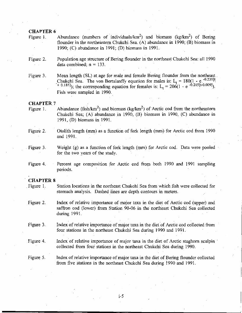
CHAPTER 6 Figure 1. Abundance (numbers of -individuals/km2) and biomass (kg/km2) of Bering

flounder in the northeastern Chukchi· Sea. (A) abundance in 1990; (B) biomass in 1990; (C) abundance in 1991; (D) biomass in 1991.

Figure 2. Population age structure of Bering flounder in the northeast Chukchi Sea: all 1990 data combined; n = 133.

Figure 3. Mean length (SL) at age for male and female Bering flounder from the northeast, _Chukchi Sea. The von Bertalanffy equation for males is: Lt = 180(1 - e. -0.230[t, + 0.185]); the corresponding equation for females is: L = 206(1 - e -0.215[t-0.009]).

t Fish were sampled in 1990.

CHAPTER 7 Figure 1. AbUndance (fish/km2) and biomass (kg/km2) of Arctic cod from the northeastern

Chukchi Sea; (A) abundance in 1990, (B) biomass in 1990, (C) abundance in 1991, (D) biomass in 1991.

Figure 2. Otolith length (mm) as a function of fork length (mm) for Arctic cod from 1990 and 1991.

. Figure 3. Weight (g) as a function of fork length (mm) for Arctic cod. Data were pooled for the two years of the study.

Figure 4. Percent age composition for Arctic cod from both 1990 and 1991 sampling periods.

CHAPTER 8 . Figure 1. Station locations in the northeast Chukchi Sea from which fish were collected for

stomach analysis. Dashed lines are depth contours in meters.

Figure 2. Index of relative importance of major taxa in the diet of Arctic cod (upper) and saffron cod (lower) from Station 90-06 in the northeast Chukchi Sea collected during 1991.

Figure 3. Index of relative importance of major taxa in the diet of Arctic cod collected from fouf stations in the northeast Chukchi Sea during 1990 and 1991.

Figure 4. Index of relative importance of major taxa in the diet of Arctic staghorn sculpin' collected from four stations in the northeast Chukchi Sea during 1990.

Figure 5. Index of relative importance of major taxa in the diet of Bering flounder collected. .

from five stations in the northeast Chukchi Sea during 1990 and 1991.

i-5

I I

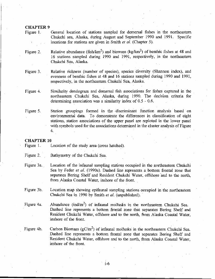
CHAPTER 9 Figure 1. General location of stations ~ampled for demersal· fishes in the northeastern .

. Chukchi sea, Alaska, during August and September 1990 and 1991. Specific locations for stations are given in Smith et al. (Chapter 5).

Figure 2. Relative abundance (fishlkm2) and biomass (kg/km2) of benthic fishes at 48 and

16 stations sampled during 1990 and 1991, respectively, in the northeastern Chukchi Sea, Alaska.

Figure 3. Relative richness (number of species), species diversity (Shannon index), and .. evenness of benthic fishes at 48 and 16 stations sampled during 1990 and 1991,

respectively, in the northeastern Chukchi Sea, Alaska.

Figure 4. Similarity dendogram and demersal fish associations for fishes captured in the northeastern Chukchi Sea, Alaska, during 1990. The decision cri!eria for determining association was a similarity index of 0.5 - 0.6.

Figure 5. Station groupings formed in the· discriminant function analysis· based· on environmental data. To demonstrate the differences in classification of eight stations, station associations of the upper panel are reploted in the lower panel with symbols used for the associations determined in the cluster analysis ofFigure 4.

CHAPTER 10 Figure 1. Location of the study area (cross hatched).

Figure 2. Bathymetry of the Chukchi Sea.

Figure 3a. Location of the infaunal sampling stations occupied in the northeastern Chukchi Sea by Feder et ai. (1990a). Dashed line represents a bottom frontal zone that separates Bering Shelf and Resident Chukchi Water, offshore-and to the north, from Alaska Coastal Water, inshore of the front. .

Figure 3b. Location map showing epifaunal sampling stations occupied in the ,northeastern Chukchi Sea in 1990 by Smith et al.· (unpublished).

Figure 4a. Abundance (indlm2) of infaunal mollusks in the northeastern Chukchi Sea. Dashed line represents a bottom frontal zone that separates Bering Shelf and Resident Chukchi Water, offshore and to the north, from Alaska Coastal Water, inshore of the front. .

Figure 4b. Carbon Biomass (gC/m2) of infaunal mollusks in the northeastern Chukchi Sea.

Dashed line represents a bottom frontal zone that separates Bering Shelf and .. Resident Chukchi Water, offshore and to the north, from Alaska Coastal Water, inshore of the front.

i-6

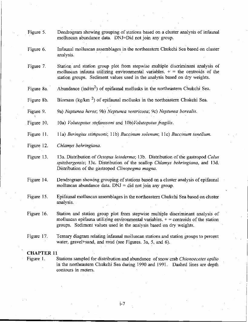
· Figure 5. Dendrogram showing grouping of stations based on a cluster analysis of infaunal molluscan abundance data. DNJ=Did not join any group.

Figure 6. Infaunal molluscan assemblages in the northeastern Chukchi Sea based on cluster analysis.

Figure 7. Station and station group plot from stepwise multiple discriminant analysis of molluscan infauna utilizing environmental. variables. + = the centroids· of the station groups. Sediment values used in the analysis based on dry weights.

Figure 8a. Abundance (ind/m2) of epifaunal mollusks in the northeastern Chukchi Sea.

Figure 8b. Biomass (kg/km 2) of epifaunal mollusks in the northeastern Chukchi Sea.

Figure 9. 9a) Neptunea heros; 9b) Neptunea ventricosa; 9c) Neptunea borealis. 1

Figure 10. lOa) Volutopsius stefanssoni and lOb)Volutopsius fragilis.

Figure 11. 11 a) Beringius stimpsoni; 11 b) Buccinum solenum; 11 c) Buccinum tenellum.

Figure 12. Chlamys behringiana.

Figure 13. 13a. Distribution of Octopus leioderma; 13b. Distribution of the gastropod Colus spitzbergensis; l3c. Distribution of the scallop Chlamys behringiana, and 13d. Distribution of the gastropod Clinopegma magna.

Figure 14. Dendrogram showing grouping of stations based on a cluster analysis of epifaunal molluscan abundance data. DNJ = did not join any group. .

Figure 15. Epifaunal molluscan assemblages in the northeastern Chukchi Sea based on cluster analysis.

Figure 16. Station and station group plot from stepwise multiple discriminant analysis of molluscan epifauna utilizing environmental variables. + = centroids of the station groups. Sediment values used in the analysis based on dry weights.

Figure 17. Ternary diagram relating infaunal molluscan stations and station groups to percent water, gravel+sand, and mud (see Figures. 3a; 5, and 6). . . .

CHAPTER 11 Figure 1. Stations sampled for distribution and abundance of snow crab Chionoecetes opilio

in the northeastern Chukchi Sea during 1990 and 1991. Dashed lines are depth contours in meters.

i-7

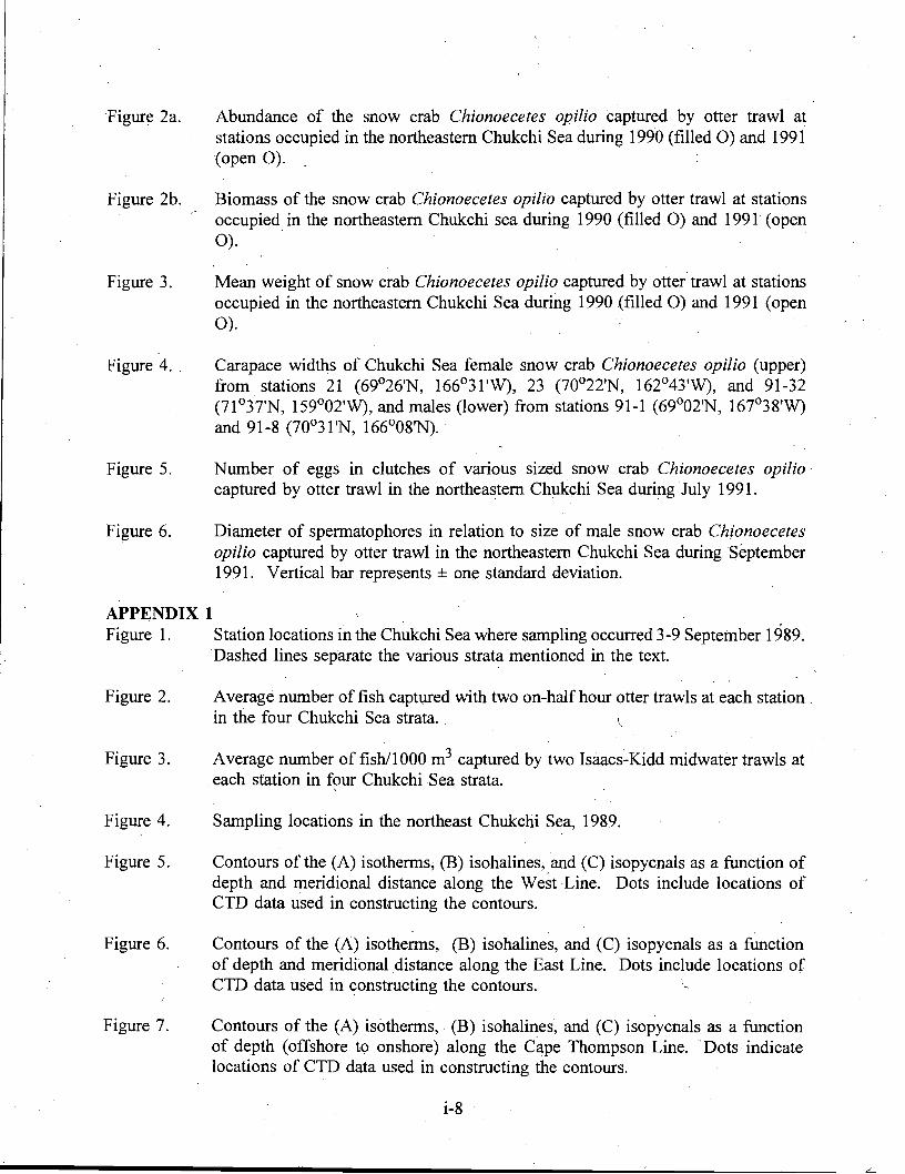
Figure 2a. Abundance of the snow crab Chionoecetes opilio captured by otter trawl at stations occupied in the northeastern Chukchi Sea during 1990 (filled 0) and 1991 (open 0). .

Figure 2b. Biomass of the snow crab Chionoecetes opilio captured by otter trawl at stations occupiedin the northeastern Chukchi sea during 1990 (filled 0) and 1991 (open 0).

Figure 3. Mean weight of snow crab Chionoecetes opilio captured by otter trawl at stations occupied in the northeastern Chukchi Sea during 1990 (filled 0) and 1991 (open 0).

Figure 4.. Carapace widths of Chukchi Sea female snow crab Chionoecetes opilio (upper) from stations 21 (69°26'N, 166°31'W), 23 (70022'N, 162°43'W), and 91-32 (71 °3TN, 159°02'W), and males (lower) from stations 91-1 (69°02'N, 167°38'W) and 91-8 (70031'N, 166°08'N).

Figure 5. Number of eggs in clutches of various sized snow crab Chionoecetes opilio captured by otter trawl in the northeastern Chukchi Sea duringJuly 1991.

Figure 6. Diameter of spermatophores in relation to size of male snow crab Chionoecetes opilio captured by otter trawl in the northeastern Chukchi Sea during September 1991. Vertical bar represents ± one standard deviation..

APPENDIX 1 Figure 1. Station locations in the Chukchi Sea where sampling occurred 3-9 September 1989.

.Dashed lines separate the various strata mentioned in the text.

Figure 2. Average number offish captured with two on-half hour otter trawls at each station. in the four Chukchi Sea strata..

Figure 3. Average number of fish/1000 m3 captured by two Isaacs-Kidd midwater trawls at .each station in four Chukchi Sea strata. ,

Figure 4. Sampling locations in the northeast Chukchi Sea, 1989.

Figure 5. Contours of the (A) isotherms; (B) isohalines, and (C) isopycnals as a function of depth and meridional distance along the West Line. Dots include locations of CTD data used in constructing the contours.

Figure 6. Contours of the (A) isotherms, (B) isohalines, and (C) isopycnals as a function of depth and meridional distance along the East Line. Dots include locations of CTD data used in constructing the contours.

Figure 7. Contours of the (A) isotherms, . (B) isohalines, and (C) isop'ycnals as a function of depth (offshore to onshore) along the Cape Thompson Line. .Dots indicate locations of CTD data used in constructing the contours.

i-8

APPENDIX 2· Figure 1. Pictorial presentation of stations proposed ("+") and those subsequently occupied

(numbered in sequence of occupation) in the northeastern Chukchi Sea during the 1990 cruise.~- .

APPENDIX 3 Figure 1. Station locations occupied during the 1991 .northeastern Chukchi Sea field season.

. Circles are stations occupied from the Oshoro Maru, triangles are stations . occupied from the Ocean Hope III, and asterisks are locations of current meter

moorings.

Figure 2. Locations proposed for current meter moorings (squares) in the northeastern Chukchi Sea during the 1991 field season shown in relation to where current meters were moored (triangles) because of heavy ice conditions in proposed areas.

APPENDIX 4 Figure 1. General stations locations occupied by the Ocean Hope III (triangles) and the

Oshoro Maru (circles) in the northeast Chukchi Sea during 1991. . Specific locations for Ocean Hope III stations are given in Smith et ai., C~apter 5. Open circles indicate stations sampled from the Oshoro Maru, triangles stations sampled from Ocean Hope III, and asterisks current meter moorings.

APPENDIX 5 Figure 1. Track of Alpha Helix during the physical oceanographic cruise of September and

October 1992.

APPENDIX I, APPENDIX 5 ~

Figure 1. JapaneselRussian/American 1992 Chukchi Sea Cruise; Alpha Helix #166 HX166 9/20-10/4, 1992.

APPENDIX II, APPENDIX 5 Figure 1a, b.

i-9

LIST OF TABLES

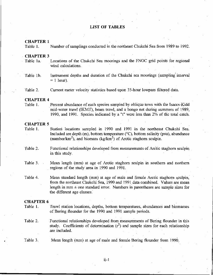
CHAPTER 1 Table 1. Number of samplings conducted in the northeast Chukchi Sea from 1989 to 1992.

CHAPTER 3 Table 1a. Locations of the Chukchi Sea moorings and the FNOC grid points for regional

wind calculations..

Table lb. Instrument depths and duration of the Chukchi sea moorings (samp1ing( interval = 1 hour).

Table 2. Current meter velocity statistics based upon 35-hour lowpass filtered data.

CHAPTER 4 .Table 1. Percent abundance ofeach species sampled by oblique tows with the Isaccs-Kidd

mid-water trawl (IKMT), beam trawl, and a bongo net during summers of 1989, 1990, and 1991. Species indicated by a "t"were less than 2% of the total catch.

CHAPTER 5 Table 1. Station locations sampled in 1990 and 1991 in the northeast Chukchi Sea.

Included are depth (m), bottom temperature (OC), bottom salinity (psu), abundance (number/km2), and biomass (kg/km2) of Arctic staghom sculpin. .

'Fable 2. Functional relationships developed from measurements of Arctic staghom sculpin . in this study.

Table 3. Mean length (mm) at age of Arctic staghom sculpin insouthem and northem . regions of the study area in 1990 and 1991. .

Table 4. Mean standard length (mm) at age of male and female Arcticstaghom s"culpin, from the northeast Chukchi Sea, 1990 and 1991. data combined. Values are mean length in mm ± one standard error; Numbers in parentheses are sample sizes for the different age classes.

CHAPTER 6 Table 1. Trawl station locations, depths, bottom temperatures, abundances and biomasses

of Bering flounder for the 1990 and 1991 sample periods.

Table 2. Functional relationships developed from measurements of Bering flounder in this study. Coefficients of determination (?) and sample sizes for each relationship are included. .

Table 3. Mean length (mm) at age of male and female Bering flounder from 1990~

ii-l

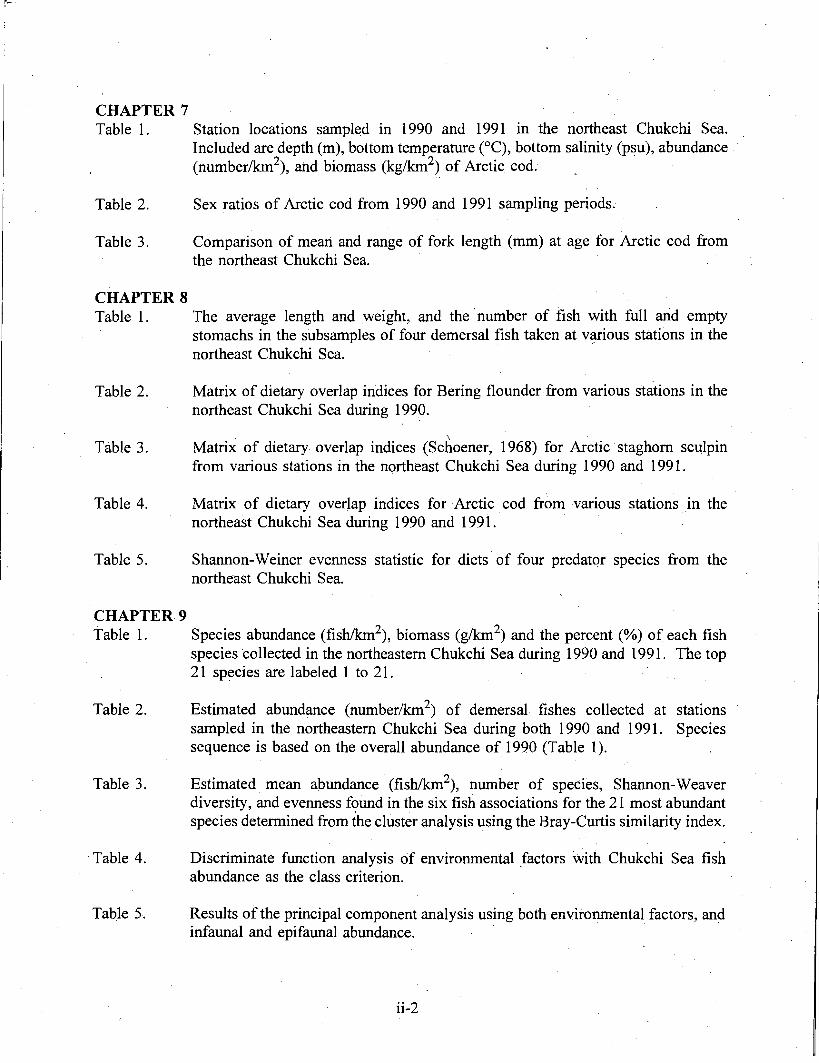
CHAPTER 7 Table 1. Station locations sampled in 1990 and 1991 in the northeast Chukchi Sea.

Included are depth (m), bottom temperature (OC), bottom salinity (psu), abundance.' (number/km2), and biomass (kg/km2) of Arctic cod.. .

Table 2. Sex ratios of Arctic· cod from 1990 and 1991 sampling periods.

Table 3. Comparison of mean and range of fork length (mm) at age for Arctic cod from the northeast Chukchi Sea.

CHAPTER 8 Table 1. The average length and weight, and the 'number of fish with full and empty

stomachs in the subsamples of four demersal fish taken at v¥ious stations in the northeast Chukchi Sea.

Table 2. Matrix of dietary overlap indices for Bering flounder·from various stations in the northeast Chukchi Sea during 1990.

\

Table 3. Matrix of dietary overlap indices (Schoener, 1968) for Arctic staghorn sculpin from various stations in the northeast Chukchi Sea during 1990 and 1991.

Table 4. Matrix of dietary overlap indices for Arctic .cod from various stations in the northeast Chukchi Sea during 1990 and 1991.

Table 5. Shannon-Weiner evenness statistic for diets of four predator species from the northeast Chukchi Sea.

CHAPTER 9 Table 1. Species abundance (fish/km2), biomass (g/km2) and the percent (%) of each fish

species 'collected in the northeastern Chukchi Sea during 1990 and 1991. The top 21 species are labeled 1 to 21.

Table 2. Estimated abundance (number/km2) of demersal fishes collected at stations sampled in the northeastern Chukchi Sea during both 1990 and 1991. . Species sequence is based on the overall abundance of 1990 (Table 1).

Table 3. Estimated mean abundance' (fish/km2), number of species, Shannon-Weaver diversity, and evenness found in the six fish associations for the 21 most abundant species determined from the cluster <:malysis using the Bray-Curtis similarity index.

.Table 4. Discriminate function analysis of environmental factors with Chukchi Sea fish abundance as the class criterion.

Table 5. Results of the principal component analysis using both environmental factors, and infaunal and epifaunal abundance.

ii-2

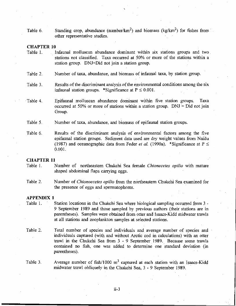
Table 6. Standing crop, abundance (number/km2) and biomass (kg/km2) for fishes from .. other representative studies.

CHAPTER 10 Table 1. Infaunal molluscan abundance dominant within six stations groups and two.

stations not classified. Taxa occurred at 50% or more of the stations within a station group. DNJ=Did not join a station group.

Table 2. Number of taxa, abundance, and biomass of infaunal taxa, by station group.

Table 3. Results of the discriminant analysis ofthe environmental conditions among the six infaunal station groups. *Significance at P:::; 0.001.

.Table 4. Epifaunal molluscan abundance dominant within five station groups. Taxa occurred at 50% or more of stations within a station group. DNJ = Did not join Group.

Table 5. Number of taxa, abundance, and biomass of epifaunal station groups.

Table 6. Results of the discriminant analysis of environmental factors among the five epifaunal station groups. Sediment data used are dry weight values from Naidu (1987) and oceanographic data from Feder eta!. (I 990a). *Significance at P :::; 0.001.

CHAPTER 11 Table 1. Number of northeastern Chukchi Sea female Chionecetes opilio with. mature

shaped abdominal flaps carrying eggs.

Table 2. Number of Chionoecetes opilio from the northeastern Chukchi Sea examined for the presence of eggs and spermatophores.

APPENDIX 1 Table I. Station locations in the Chukchi Sea Where biological sampling occurred from 3 ­

9 September 1989 and those sampled by previous authors (their stations are in parentheses). Samples were obtained from otter and Isaacs-Kidd rilidwater trawls at all stations and zooplankton samples at selected stations.

Table 2. Total number of species and individuals and average number of species and individuals captured (with and without Arctic cod in calculations) with an otter trawl in the Chukchi Sea from 3 - 9 September .1989.. Because some trawls contained no fish, one was added to determine one standard deviation (in parentheses).

Table 3. Average number of fish/IOOO m3 captured at each station with an Isaacs-Kidd midwater trawl obliquely in the Chukchi Sea, 3 - 9 September 1989. ­

ii-3

Table 4. Total number of species and individuals captured and average number of species and individuals 1000 m3 (including and excluding Arctic cod in calculations) with Isaacs-Kidd midwater trawl (IKTM) in the Chukchi Sea strata from 3 - 9 September 1989. One was added to each IKTM to determine one standard deviation (in parentheses).

Table 5. Invertebrates collected with an otter trawl in the Chukchi Sea, 3 - 9 September 1989.

Table 6. Morphometric relationships in four species of zoarcid fishes from the northeast Chukchi Sea. Abbreviations are as follows: GO = length of gill opening; HL = head length; HW = head width; 10 = interorbital width; n = sample size; PA ~

preanal length; Pe = pectoral length; PL = pelvic length; TL = total length. Each proportion is multiplied by 100. Values are mean ± one' standard deviation and range in parentheses. Length in mm.

Table 7. Meristic characters in four' species of zoarcids from the northeast Chukchi Sea. Abbreviations are as follows: LT == number of lower jaw teeth; PR := number of pectoral fin rays; PT = number of palatine teeth; UT = number of upper jaw teeth; VT = number of vomerine teeth.

.Appendix Table 1. Numbers of each species of fish captured In one-half-hour otter trawls, 3-9

_September 1989 from the Chukchi Sea.

Appendix Table 2. Numbers of each species of fish captured in an Isaacs-Kidd rviidwater Trawl (lKMT) in the Chukchi' Sea during 3-9 September 1989.

Appendix Table 3. Numbers of each species of fish/lOOO m3 captured in an Isaacs-Kidd Midwater Trawl (IKMT) in the Chukchi Sea during 3-9 September 1989.

APPENDIX 2 Table 1. Nominal list of fish species captured by otter trawl during 1989 and 1990 Chukchi

Sea cruises. the 1989 cruise included sampling in'the southeast Chukchi Sea whereas sampling in 1990 was only in the northeastern portion. "x" indicates year of capture.

Table 2. List of mollusk species captured in the Chukchi Sea during 1989 and 1990. The 1989 cruise included sampling in the northeast and southeast Chukchi Sea and were captured by otter trawl to which a srhall dredge was attached on an otter board. They were captured only by otter trawl in the northeast Chukchi Sea in 1990. They were identified by Rae Baxter.

APPENDIX 3 Table 1. Station locations in the northeastern Chukchi Sea occupied from the Oshoro Maru

(OM) on 25-31 July and from the Ocean Hope IlIon 12-23 September 1991.

Table 2. Proposed and actual locations of current meter moorings deployed in the northeastern chukchi Sea iIi September and October 1991.

Table J. List of fish species captured by otter trawl in the northeastern Chukchi Sea in 1989 and nominal species of those captured in 1990 and 1991 ("x" indicates year).

Table 4. List of invertebrates captured by otter trawl in the northeastern Chukchi Sea in I .1991 from the Ocean Hope III.

APPENDix 4 Table 1. Station locations sampled in 1991 and 1992 in the northeast Chukchi Sea by the

Oshoro Maru.

Table 2. Number of each species caught from the Dshoro Maru by otter trawl in the northeast Chukchi Sea in 1991.

Table 3. Number of fish captured from the Oshoro Maru by otter trawl in the northeast Chukchi Sea in 1992.

Table 4. The total number of fish captured at each station in the northeast Chukchi Sea by otter trawl from two different vessels in 1991. The total from the Ocean Hope III is the sum of two 30 min hauls while the total from Oshoro Maru is the sum from one 60 min haul.

APPENDIX 5 Table 1. Stations sampled from the Oshofo Maru with an otter trawl in the northeastern

Chukchi Sea in July 1992. Station location is the latitude and.longitude when the otter trawl reached' the bottom. Distance is the distance trawled. Previous sampling column indicates year and from which ~hip '(OM = Oshoro Ma~u and OR = Ocean Hope III) at locations near where previous sampling occurred.

APPENDIX I, APPENDIX 5 Table 1. HX166 CTDF Station list.

Table 2. Current Meter Moorings Recovered.

Table 3. Current Meter Moorings Deployed.

Table 4. Sea-ice stations and activities.

Table 5. Stations sampled for radioactivity.

ii-5

APPENDIX II, APPENDIX 5 Table 1. Total numbers of marine mammals recorded during cruise HX-166.

APPENDIX 6 . Table 1. Number of samples taken by each gear type.

Table 2. Number of fish found in bongo net samples. Left indicates the left net, and right the right net. Sample period 1 was July while 2 waS in August.

Table 3. Number of fish found in IKMT samples. Sample period 1 was in J~ly while 2 was in August. .

Table 4. Volume of water (m3) sampled by bongo net in the northeast Chukchi Sea.

LITERATURE CITED

APPENDICES

ii-6

/

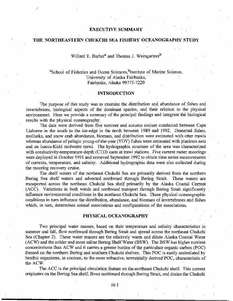
EXECUTIVE SUMMARY

THE NORTHEASTERN CHUKCHI SEA FISHERY OCEANOGRAPHY STUDY

Willard E. Barbera and Thomas J. Weingartnerb

aSchool of Fisheries and Ocean Sciences,b1nstitute of Marine Science, University of Alaska Fairbanks,· Fairbanks, Alaska 99775-7220

INTRODUCTION

The purpose of this study was to examine the distribution and abundance of fishes and invertebrates, biological aspects of the dominant· species, and their relation to· the physical environment. Here we provide a summary of the principal findings and integrate the biological results with the physical oceanography.

The data were derived from five summer and autumn· cruises conducted between Cape Lisburne in the south to the ice-edge in the north between 1989 and 1992. Demersal fishes, mollusks, and snow crab abundance, biomass, and distribution were estimated with otter trawls whereas abundance of pelagic young-of-the-year (YOY) fishes were estimated with plankton nets and an Isaccs-Kidd midwater trawl. The hydrographic structure of the area was characterized with conductivity-temperature':'depth (CTD) casts at trawl stations. Five current meter moorings were deployed in October 1991 and retrieved September 1992 to obtain time series measurements of currents, temperature, and salinity. Additional hydrographic data were also collected during the mooring recovery cruise. .

The shelf waters of the northeast Chukchi Sea are primarily derived from the northern Bering Sea shelf waters and advected northward through Bering Strait. These waters are transported across the northeast Chukchi Sea shelf primarily by the Alaska Coastal Current

. (ACC).. Variations in both winds and northward transport through Bering Strait significantly influence environmental conditions in the northeast Chukchi Sea. These physical oceanographic conditions in tum influence the distribution, abundance, and biomass of invertebrates and fishes which, in turn, determines animal associations and configurations of the associations.

PHYSICAL OCEANOGRAPHY

Two principal water masses, based on their temperature and salinity characteristics in summer and fall, flow northward through Bering Strait and spread across the northeast Chukchi Sea (Chapter 2). These water masses are the relatively warm and dilute Alaska Coastal Water (ACW) and the colder and more saline Bering Shelf Water (BSW). The BSW has higher nutrient concentrations than ACW and it carries a greater burden of the particulate organic carbon (POC) formed on the northern Bering and southern Chukchi shelves. This POC is easily assimilated by benthic organisms, in contrast, to the more refractive, terrestrially derivedPOC, characteristic of the ACW.

The ACC is the principal circulation feature on the.northeast Chukchi shelf. This current originates on the Bering Sea shelf, {lows northward through Bering Strait, and drains the Chukchi

iii-l

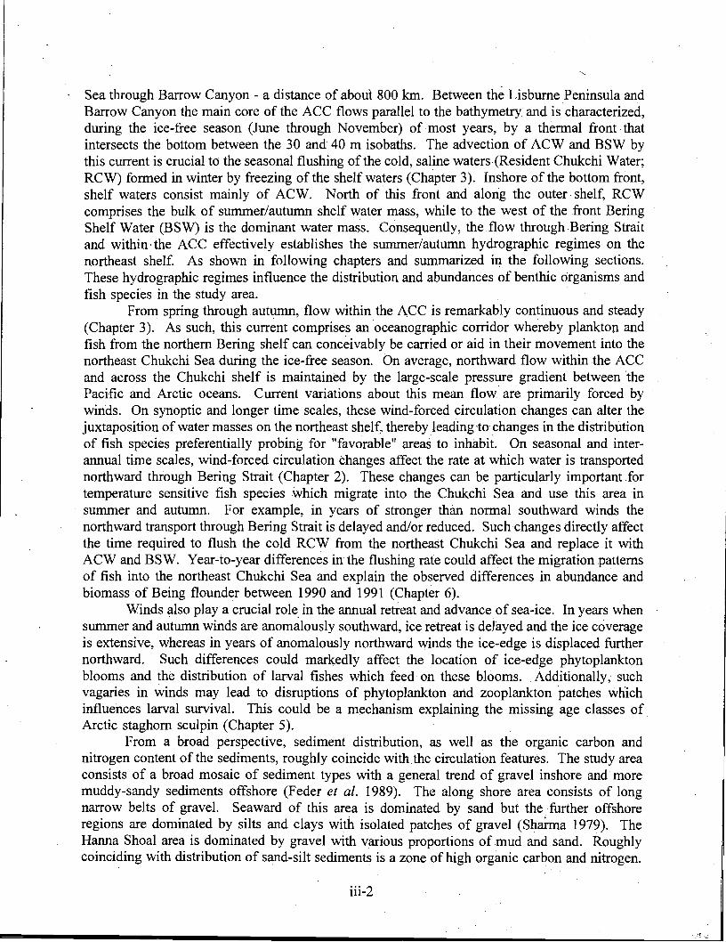
Sea through Barrow Canyon - a distance of about 800 km. Between the Lisburne Peninsula and Barrow Canyon the main core of the ACC flows parallel to the bathymetry and is characterized, during the ice-free season (June through November) of most years, by a thermal front that intersects the bottom between the 30 and 40 m isobaths. The advection of ACW and BSW by this current is crucial to the seasonal flushing ofthe cold, saline waters(Resident Chukchi Water; RCW) formed in winter by freezing of the shelf waters (Chapter 3). Inshore of the bottom front, shelf waters consist mainly of ACW. North of this front and along the outer· shelf, RCW comprises the bulk of summer/autumn shelf water mass, while to the west of the front Bering Shelf Water (BSW) is the dominant water mass. Consequently, the flow through Bering Strait and within-the ACC effectively establishes the summer/autumn hydrographic regimes on the northeast shelf. As shown in following chapters and summarized in the following sections. These hydrographic regimes influence the distribution and abundances of benthic organisms and fish species in the study area.

From spring through autumn, flow within the ACC is remarkably continuous and steady (Chapter 3). As such, this current comprises an oceanographic corridor whereby plankton and fish from the northern Bering shelf can conceivably be carried or aid in their movement into the northeast Chukchi Sea during the ice-free season. On average, northward flow within the ACC and across the Chukchi shelf is maintained by the large-scale pressure gradient between ·the Pacific and Arctic oceans. Current variations about this mean flow are primarily forced by winds. On synoptic and longer time scales, these wind-forced circulation changes can alter the juxtaposition of water masses on the northeast shelf, thereby leading to changes in the distribution of fish species preferentially probing for "favorable" areas to inhabit. On seasonal and inter­annual time scales, wind-forced circulation changes affect the rate at which water is transported northward through Bering Strait (Chapter 2). These changes can be particularly important for temperature sensitive fish species which migrate into the Chukchi Sea and use this area in summer and autumn. For example, in years of stronger than normal southward winds the northward transport through Bering Strait is delayed and/or reduced. Such changes directly affect the time required to flush the cold· RCW from the northeast Chukchi Sea and replace it with ACW and BSW. Year-to-year differences in the flushing rate could affect the migration patterns of fish into the northeast Chukchi Sea and explain the observed differences in abundance and biomass of Being flounder between 1990 and 1991 (Chapter 6).

Winds also playa crucial role in the annual retreat and advance of sea-ice. In years when . . summer and autumn winds are anomalously southward, ice retreat is delayed and the ice coverage is extensive, whereas in years of anomalously northward winds the ice-edge is displaced further northward. Such differences could markedly affect the location of ice-edge phytoplankton blooms and the distribution of larval fishes which feed on these blooms. Additionally, such vagaries in winds may lead to disruptions of phytoplankton and zooplankton patches which influences larval survival. This could be a mechanism explaining the missing age classes of. Arctic staghorn sculpin (Chapter 5).

From a broad perspective, sediment distribution, as well as the organic carbon and nitrogen content of the sediments, roughly coincide with .the circulation features. The study area consists of a broad mosaic of sediment types with a general trend of gravel inshore and more muddy-sandy sediments offshore (Feder et al. 1989). The along shore area consists of long narrow belts of gravel. Seaward of this area is dominated by sand but the further offshore regions are dominated by silts and clays with isolated patches of gravel (Shaima 1979). The· Hanna Shoal area is dominated by gravel with various proportions of mud and sand. Roughly coinciding with distribution of sand-silt sediments is a zone of high organic carbon and nitrogen.

iii-2

There is also a narrow band of sediments characterized by relatively high organic carbon (>7 mg/l) and nitrogen (>0.8 mg/l) which progresses northwestward from the Point Hope and Cape . Lisburne area to offshore. Additionally, there is a wide band of sediments of high organic' content emanating from the Point Franklin area northwestward offshore (Feder et al. 1989).

DISTRIBUTIONS AND ASSOCIATIONS OF BlOTA

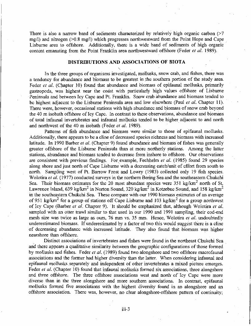
In the three groups of organisms investigated, mollusks, snow crab, and fishes, there was a tendency for abundance and biomass to be greatest in Jhe southern portion of the study area. Feder et al. (CJ1apter 10) found that abundance and biomass of epifaunal mollusks, primarily gastropods, was highest near the coast with particularly high values offshore. of Lisburne Peninsula and between Icy Cape and Pt. Franklin. Snow crab abundance and biomass tended to be highest adjacent to the Lisburne Peninsula area and low elsewhere (Paul et al. Chapter 11). There were, however, occasional stations with high abundance and biomass of snow crab beyond the 40 m isobath offshore of Icy Cape.. In contrast to these observations, abundance and biomass of total infaunal invertebrates and infaunal mollusks tended to be higher adjacent to and north and northwest of the 40 m isobath (Feder et al. 1989).

Patterns of fish abundance and biomass were similar to those of epifaunal mollusks. Additionally, there appears to be a cline of decreased species richness and biomass with increased latitude.. In 1990 Barber et al. (Chapter 9) found abundance and biomass of fishes was generally greater offshore of the Lisburne Peninsula than at more northerly stations. Among the latter stations, abundance and biomass tended to decrease from inshore to 'offshore. Our observations are consistent with previous findings. For, example,Fechhelm et al. (1985) found 29 species along shore and just north of Cape Lisburne with a decreasing catch/unit of effort from south to north. Sampling west of Pt. Barrow Frost and Lowry (1983) collected only 19 fish species. Wolotiraet al. (1977) conducted surveys in the northern Bering Sea and the southeastern Chukchi Sea. Their biomass estimates for the 20 most abundant ~ecies were 351 kg/km2 north of St. Lawrence Island, 639 kg/km2 in Norton Sound, 320 kg/km in Kotzebue Sound, and 158 kg/km2

in the southeastern Chukchi Sea. These compare with our 1990 biomass estimates of an average of 951 kg/km2 for a group of stations off Cape Lisburne and 103 kg/km2 for a group northwest of Icy Cape (Barber et al. Chapter 9). It should be emphasized that, although Wolotira et al. sampled with an otter trawl similar to that used in our 1990 and 1991 sampling, their cod-end mesh size was twice as large as ours, 76 mm vs. 35 mm. Hence, Wolotira et al. undoubtedly underestimated biomass. If underestimated by a factor of two this would suggest there is a cline of decreasing abundance with increased latitude. They also found that biomass was higher nearshore than offshore.

Distinct associations of invertebrates and fishes were found in the northeast Chukchi Sea aDd there appears. a qualitative similarity between the geographic configurations of those formed . by mollusks and fishes. Feder et al. (1989) found two alongshore and two offshore macrofaunal associations and the former had higher diversity than the latter. When considering infaunal and epifaunal mollusks separately and independent of other invertebrates a mixed picture emerges. Feder et al. (Chapter 10) found that infaunal mollusks formed six associations, three alongshore and three offshore. The three offshore associations west and north" of Icy Cape were more diverse than in the three alongshore· and more southern associations. In contrast, epifaunal mollusks formed five associations with the highest diversity found in an alongshore and an offshore association. There was, however, no clear alongshore-offshore pattern of continuity;

iii-3

both alongshore and offshore associations were disjointed. Additionally, the offshore associations were interspersed with areas characteristic of one alongshore association.

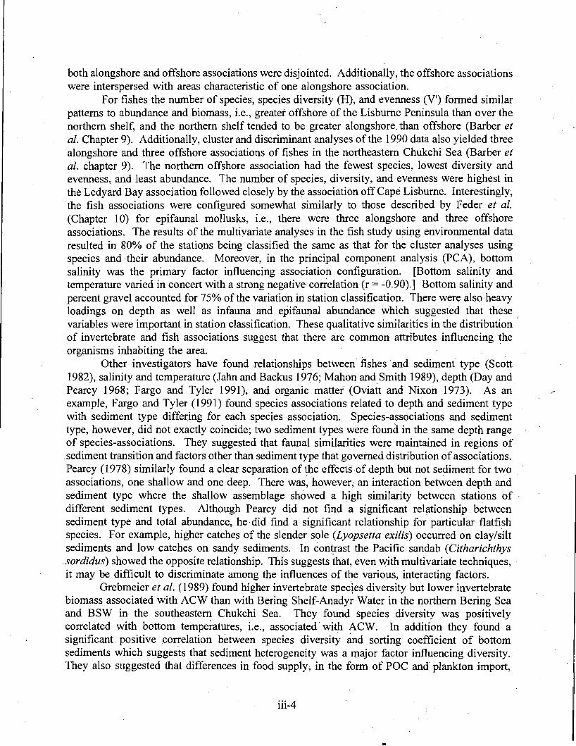
For fishes the number of species, species diversity (H), and evenness (V') formed similar patterns to abundance and biomass, i:e., greater offshore of the Lisburne Peninsula than over the northern shelf, and the northern shelf tended to be greater alongshore. than offshore (Barber et al. Chapter 9). Additionally, cluster and discriminant analyses of the 1990 data also yielded three alongshore and three offshore associations of fishes in the northeastern Chukchi Sea (Barber et al. chapter 9). The northern offshore association had the fewest species, lowest diversity and evenness, and least abundance. The number of species, diversity, and evenness were highest in the Ledyard Bay association followed closely by the association off Cape Lisburne. Interestingly, the fish associations were configured somewhat similarly to those described by Feder et al. (Chapter 10) for epifaunal. mollusks, i.e., there were three alongshore and three offshore associations. The results of the multivariate analyses in the fish study using environmental data resulted in 80% of the statiQns being classified the same as that for the cluster analyses using species and their abundance. Moreover, in the principal component analysis (PCA), bottom salinity was the primary factor influencing association configuration. [Bottom salinity and temperature varied in concert with a strong negative correlation (r = -0.90).] Bottom salinity and percent gravel accounted for 75% of the variation in station classification. There were also heavy loadings on depth as well as infauna and epifaunal abundance which suggested that these variables were important in station classification. These qualitative similarities in the distribution of invertebrate and fish associations suggest that there are common attributes influencing the organisms inhabiting the area. . .

Other investigators have found .relationships between fishes' and sediment type (Scott 1982), salinity and temperature (Jahn and Backus 1976; Mahon and Smith 1989), depth (Day and Pearcy 1968; Fargo and Tyler 1991), anqorganicmatter (Oviatt and Nixon 1973). As an example, Fargo and Tyler (1991) found species associations related to depth and sediment type with sediment type differing for each species association. Species-associations and sediment type, however, did not exactly coincide; two sediment types were found in the same depth range' of species-associations. They suggested that faunal similarities were maintained in regions of .sediment transition and factors other than sediment type that governed distribution ofassociations. Pearcy (1978) similarly found a clear separation of the effects of depth but not sediment for two associations, one shallow and one deep. There was, however, an interaction between depth and sediment type where the shallow assemblage showed a high similarity between stations of . different sediment types. Although Pearcy did not find a significant relationship between sediment type and total abundance, he did find. a significant relationship for particular flatfish species. For example, higher catches of the slender sole (Lyopsetta exilis) occurred on clay/silt sediments and low catches on sandy sediments. In contrast the Pacific sandab (Citharichthys

.sordidus) showed the opposite relationship.' This suggests that, even with multivariate techniques, . it may be difficult to discriminate among the influences of the various, interacting factors.

Grebmeier et al. (1989) found higher invertebrate specles diversity but lower invertebrate biomass associated with ACW than with Bering Shelf-Anadyr Water in the northern Bering Sea and BSW in the southeastern Chukchi Sea. They found species diversity was positively correlated with bottom temperatures, i.e., associated with ACW. In addition they· found a significant positive correlation between species diversity and sorting coefficient of bottom sediments which suggests that sediment heterogeneity was a major factor influencing diversity. They also suggested that differences in food supply; in the form of POC and plankton import,

iii-4

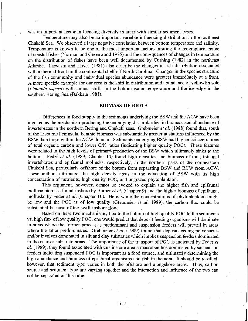
was an important factor influencing diversity in areas with similar sediment types. Temperature may also be an important variable influencing distribution in the northeast

Chukchi Sea. We observed a large negative correlation between bottom temperature and salinity. Temperature is known to be one of the most important factors limiting the geographical range of coastal fishes (Norman and Greenwood 1975) and the consequences of changes in temperature on the distribution of fishes have been well documented by Cushing (1982) in the northeast Atlantic. Laevastu and Hayes (1981) also describe the changes in fish distribution associated· with a thermal front on the continental shelf off North Carolina. Changes in the species structure of the fish community and individual species abundance were greatest immediately at a front. A more specific example for our area is the shift in distribution and abundance of yelloWfih sole. (Limanda aspera) with annual shifts in the bottom water temperature and the ice edge in the southern Bering Sea (Bakkala 1981).

BIOMASS OF BIOTA

Differences in food supply to the sediments undedying the BSW and the ACW have been invoked as the mechanism producing the underlying dissimilarities in biomass and abundance of invertebrates in the northern Bering and Chukchi seas. Grebmeier et al. (1988) found that, south of the Lisburne Peninsula, benthic biomass was substantially greater at stations influenced by the BSW than those within the ACW domain. Sediments undedying BSW had higher concentrations of total organic carbon and lower C/N ratios (indicating higher quality POC). These features were related to the high levels of primary production of the BSW which ultimately sinks to the bottom. Feder et al. (1989; Chapter 10) found high densities and biomass of total infaunal invertebrates and epifaunal mollusks, respectively, in the northern parts of the northeastern Chukchi Sea, particularly offshore of the bottom front separating BSW and RCW from ACW.. These authors attributed the high density· areas to the advection of BSW with its high concentration of nutrients, high quality POC, and ungrazed phytoplankton.

This argument, however, cannot be evoked. to explain the higher fish and epifaunal mollusc biomass found inshore by Barber et al. (Chapter 9) and the higher biomass of epifaunal mollusks by Feder etal. (Chapter 10). Here, while the concentrations of phytoplankton might be low and the POC is of low quality (Grebmeier et al. 1989), the carbon flux could be substantial· because of the swift inshore flow.

Based on these two mechanIsms, flux to the bottom of high quality POC to the sediments vs. high flux of low quality POC, one would predict that deposit feeding organisms will dominate in areas where the former process is predominant· and suspension feeders will prevail in areas where the latter predominates. Grebmeier et al. (1989) found that deposit-feeding polychaetes and/or bivalves dominated in silt and clay substrates which implies suspension feeders dominated in the coarser substrate areas. The importance of the transport of POC is indicated by Feder et al. (1989); they found associated with this inshore area a macrobenthos· dominated by suspension feeders indicating suspended POC is important as. a food source, and ultimately determining the high abundance and biomass of epifaunal organisms and fish in the area. It should be recalled, . however, that sediment type varies in both the offshore and alongshore areas. Thus, carbon source and sediment type are varying together and the interaction and influence of the two can not be separated at this time.

iii-5

INTERANNUAL VARIABILITY

It was implied in the previous section (Physical Oceanography) and in Chapters 2 and 3 that there is considerable interannual variability in the transport of waters through the Bering Strait. The interannual variation in the physical oceanographic conditions appear to impact the abundance and distribution of fishes in the northeast Chukchi Sea. Additionally, there is support for Pruter and Alverson's (1962) hypothesis that some species· of fishes and invertebrates inhabiting the northeastern Chukchi Sea are maintained via continual recruitment of eggs and larvae transported northward from the southeastern Chukchi Sea or northeastern Bering Sea.

Biomass, abundance, and age structure of Arctic staghorn sculpin varied considerably between 1990 and 1991. Smith et al. (Chapter 5) found that mean biomass and abundance were significantly higher in 1990 than in 1991. For aU 48 stations sampled in 1990 mean abundance was 716 ± 1345 fish/km2 and mean biomass was 8.4 ± 13.5 kg/km2. Mean abundance for the 16 stations sampled in 1991 was 429 ± 776 fish/km2; mean biomass was 4.7 ± 7.8 kg/km2. Comparison of abundance and biomass values for the two sample years indicated significantly higher values for 1990 (p < 0.001). In 1990 we foun~ (Chapter 5) that 42% of the Arctic staghorn sculpin consisted of fish older thap. four years. In 1991 the number of fish in these age· categories represented only 9% of the total. The oldest female observed was 9 years old; the oldest male was 8. The age structure changed dramatically from 1990 to 1991. In 1990 41.6% of the population consisted of fish 2: 4 yearsold; 4.4% were 2: 6 years old. In contrast, in 1991 only 8.9% of the population was 2: 4 years old; only 1.4% was 2: 6 years old. Three year old· fish were· very scarce in 1990 and 4 year old fish were scarce in 1991·. suggesting that the 1987 class had very poor recruitment success. Because the stations from which fish were aged ranged from the extreme southern boundary of the study area· to far to the northeast, this possible· recruitment failure was widespread and could have resulted from a large...scaleperturbation in the> environment. Further, the marked difference in age distributions of Arctic staghorn sculpin in the two sample years suggests that variation in the physical environment may result in recruitment failures or mass mortality in this species.

Similar results were found for Bering flounder (Smith et al. Chapter 6); Both biomass and abundance were dramatically different in the two years of this study. Mean biomass declined significantly from 17.2 kg/km2 in 1990 to 0.79 kg/km2 in1991. Mean abundance estimates for all stations sampled in 1:9? and 1991. (995 and 449 fis~2, resp~ctively) differed significantlJ (D = 785; p < 0.001). SImIlarly, 1990 and 1991 mean bIOmass estImates (17.2 and 0.79 kg/km , respectively) also differed significantly (D = 825; p < 0.001). Eight stations were sampled in both field seasons. Mean abundance and biomass at these stations in 1990 (207 fish/km2; 7.6 . kg/km2, respectively) were significantly higher (D == 85; p < 0.001) than the estimates for 1991 . (19.7 fish/km2; 0.66 kg/km2, respectively). This reduced abundance and biomass in 1991 was associated with significantly lower temperatures in 1991. Comparing the eight stations common to both years we found mean bottom temperatures of 5.4 and 0.9°C, respeCtively (D = 54; p < 0.05).

Age structure of Bering flounder was also very different between 1990 and 1991. In 1990 we found (Chapter 6) that ages ranged from 1 to 11 with age class 5 dominating. This differs considerably from Pruter and Alverson (1962) who found ages ranging from 6 to 13 with ages 7 through 9 making up 90% of the total number of fish. Additionally, in 1990 we found that 75% of the Bering flounder were 2: 5 years old. This is evidence for dramatic shifts in population age structure over time as well as variability in abundance and that interannual differences in physical oceanographic conditions influence abundance of fishes in the area,

iii-6

possibly from the import from more southern waters. Wyllie-Echeverria et al. (Chapter 4) concluded that populations of Bering flounder in the

northeastern Chukchi Sea are maintained by the transport of larvae in the ACC. Sampling ichthyoplankton with a variety of mid-water gear from 1989 through 1991, Arctic cod dominated the catches and occurred throughout the northeastern Chukchi Sea; higher concentrations were found at northern stations during all three years. Arctic cod rarely occurred at southern stations when BSW was present. Bering flounder occurred primarily in areas dominated by the ACW as far north as 71 'N. They did not occur where RCW was present.

The distribution of YOY Bering flounder and two other species reflected the distribution of the water masses (Wyllie-Echeverria et al. Chapter 4). Bering flounder were present during 1989 and 1990 in ACW and ACWIBSW but absent from ACWfRCW. In (991 only one yay Bering flounder was captured and it was in ACW. Pleuronectes spp., dominated by yellowfin . sole (P. asper) , and sandlance (Ammodytes hexapterus), followed the general pattern of Bering flounder distribution. These fish are primarily distributed in the Bering Sea and extend into the Chukchi Sea (Allen and Smith 1988). In 1989 and 1990 Pleuronectes spp. yay occurred in ACW, and sandlance YOY were captured in ACW and ACW/RCW but were absent in 1991 ' samples. In 1990 the winds were primarily from the south and in 1991 from the north. The increased advection of BSW into the northeast Chukchi Sea would have increased the importof more southern species into the sampling area as compared to 1991. This suggests that YOY Bering flounder, and quite possibly yellowfin sole and sandlance, were advected into the northeastern Chukchi Sea with ACW.

To further test this hypothesis Wyllie-Echeverria et al. (Chapter 4) re-examined an earlier set of data obtained in September and October 1970 (Ingham et al. 1972). Using the data reported by Quast (1972) and the temperature and salinity profiles of Ingham and Rutland (1972) reported in this study, Wyllie-Echeverria et al. reconstructed the water masses present and yay distribution for 1970. The ACW was present nearshore and to 7l'N while RCW was not present south of 69°30'N. They found that Arctic cod were present at all stations but Bering flounder occurred only at stations south of 69°30'N and were associated with ACW. Water mass characteristics and distribution ofpelagic juvenile fish species indicate that the conditions of1970 were similar to those in 1989 and 1990. These authors concluded 'that while Bering flounder and . others may be routinely advected into the northeastern Chukchi Sea by ACW, RCW may be a critical factor in delimiting their northern distribution.

CONCLUSIONS

The physical oceanographic conditions of the study area influence the distribution, abundance, and biomass of invertebrates and fishes which, in turn, determines associations of these organisms. Highest abundance and biomass of snow crab,epifaunal mollusks, and fishes tended to be in the south. Moreover, .epifaunal mollusc abundance and biomass was highest nearer the coast. Infaunal mollusc biomass and abundance, however, was greatest adjacent to, and north and northwest of a bottom thermal front separating the Bering Shelf Water (BSW) and Resident Chukchi Water (RCW) masses from the Alaska Coastal Water (ACW). The mollusks,

. .

epifauna and infauna, and fishes formed inshore and offshore associations. These associations were affiliated with bottom type, salinity, and bottom temperature. The observed differences in abundance of YOY, missing year classes, and dramatic differences in abundance and biomass of specific fish species appear to be related to interannual differences in wind and transport.

In view of the findings, the northeastern Chukchi Sea appears to be a transition zone

iii-7

between 'the northern Bering Sea and the Arctic Ocean. The observed differences in distributions, abundance, biomass, and the resulting fish and invertebrate associations involve sediment type, the area's hydrography, import of particulate organic carbon (POC), and flux of plankton from the water column to the benthos. This shelf area may thus be considered the "downstream link" in the flow of water between the Bering Sea and the Arctic Ocean. Therefore, processes operating "upstream" in the Bering Sea have considerable influence on the physical and biological characteristics of the northeastern Chukchi Sea.

iii-8

CHAPTER 1

INTRODUCTION,BACKGROUND, AND :lVIETHODS

WILLARD E. BARBERa, RONALD L. SMITHa, and THOMAS J. WEINGARTNERb

aSchool of Fisheries and Ocean Sciences, and bInstitute of Marine Science University of Alaska Fairbanks, Fairbanks, Alaska 99775,.7220

INTRODUCTION

In the absence of commercially-exploited populations, there has been,historically, little emphasis placed on acquisition of data on the organisms and the habitats they occupy or interrelationships between the two. If little information exists on how organisms interact with . their habitat and associated fauna, it will be difficult or impossible to conceptualize or predict how fishery organisms might respond to natural or artificial perturbations. Informed management decisions depend on information and predictive capability. In the northeastern Chukchi Sea,

. exploitation has been extremely low since the end of corrimercial whaling. Very little, pertinent information existed until very recently in spite of the fact that the area is important for· subsistence fisheries and is an important migration corridor and habitat for whales, walruses and anadromous fishes.

There has been considerable interest and effort in developing information for this area over the past six years because of potential oil exploration and extraction. Much remains to be understood about exploitable species and their relation to the environment. The Outer Continental Shelf Environmental Assessment Program has recognized 'the need for this information.

This project is a result of the efforts of the Minerals Management Service (MMS) of the U.S. Department of Interior to oversee oil exploration in the study area in a manner consistent with protection of marine and coastal environments. Our environmental studies will help delineate the oceanographic environment and some basic life history characteristics of the more abundant fish and invertebrates present. We hope our studies have clarified what Arctic resources may be at risk from potential oil and gas activities and have helped assess the possible effects on these resources.

The overall goal of this project was to develop a data base that will allow characterization of the area and, in a general way, prediction of possible outcomes of environmental perturbations, whether natural or resulting from human activity. An underlying assumption is that the basic life history and biological characteristics of the dominant fish and shellfish species in the northeastern Chukchi are similar to those observed in other parts of their range or for similar species and may be used to interpret biological processes in the Chukchi Sea. The study evolved from· a single year survey to a mUlti-year study which involved the University of Alaska's vessel the Alpha Helix and a chartered trawler. It also involved ships of opportunity, launches being operated from a tender supporting drilling operations and the University of Hokkaido's research vessel the· Oshoro Maru. The general locations sampled during the four field seasons are shown in Figure 1.

1-1

,-----------------r ,,' ,----------.:...---,--------,73

l - - - - -:- - - - - - - - - - - - 8arraw . . .:·~t

..;I~.c.ape ", ­

'. . .,,:.;.:.:.' •• ·:C~~~·

•.••••• L,sbvr.... P--.sula ·Pt.•~.'

.....:... ALASKAALASKA

===f---~+,66' 155'

1989 1990 ,-----------------r 73' ,-----------------:-r. 73'

=~""""+----+66· 1------<!.~+===4---__+,66' 170· '55''55'

1991 1992

Figure 1. General sampling locations where fishes and invertebrates were sampled and . current meter moorings established during the four years of study in the northeastern Chukchi Sea. .

o 0

. '. .

::::::..... .•..: ~t~ Franklll'l

o •

• • o 0 ~-.~..,.

..

:e-Lasbu.... .;::::::-•. , 'Llsoumlt Pennsula

~Hope ... ALASKA

.~.~Y

...::::t~n Bay .

......:-:.;.;.:e-l.J5/Jl.nIe •••• ~Peftr'tsula

.pt Hof;le

":-::::}:" ':-:':'::-. ALASKA

1-2

To guide our initial thinking and data collection we fonned several hypotheses. First, we hypothesized that the physical attributes of the environment and the life history characteristics of the species are variable both temporally and spatially. Second, we hypothesized that there would be differences in abundance and/or biomass of the major species occupying the different water masses in the area. Third, we hypothesized that the fish communities relate to infaunal and eipfaunal invertebrate communities previously identified. . ,

Objectives to address these hypotheses were:

I), Detennine the distribution of water masses in the northeastern Chukchi Sea;

2) Develop basic biological infonnation for dominant fish and shellfish species for important life stages;

3) Detennine relationship between hydrographic conditions and fish speCIes abundance, biomass and/or behavior;

4) Detennine the community structure of the fish and shellfish with emphasis on ichthyofauna in the northeastern Chukchi Sea;

5) Compare community structure of fish and shellfish with previously identified infaunal invertebrate communities of the area. ­

To guide the reader, this report is organized in the following manner. First, in this introductory chapter, we review the literature which fonned the basis of our approach and thinking at the beginning of the study. We also present the general methods used and areas sampled during 'the study. Second, because we felt strongly that the knowledge gained in'this project should be disseminated as widely as possible, the remaining. chapters are based on manuscripts submitted (or in final preparation) to refereed scientific journals or a symposium on the ecology of arctic fishes. Chapter 2 reviews what was known about the oceanography of the study area with additional infonnation gained from oceanographic observations at stations occupied primarily for biological sampling. Chapter J presents new infonnation on the physical oceanography from hydrographic and five current meter stations established in the study area. Chapter 4 presents infonnation on the relationship of young-of-the-year fishes to the water. masses ofthe area. Chapters 5, 6, and 7 presents new infonnation on the distribution, abundance, and biology of three dominant species which occupy the area, the Arctic staghorn sculpin (Gymnocanthus tricuspis), the Bering flounder (Hippoglossoides robustus), and the Arctic cod (Boreogadus saida). Chapter 8 presents infonnation on the food habits of these three species and saffron· cod (Eleginus gracilis). Chapter 9 concerns the fish community of the area and its relationship to the physical oceanography. Chapter 10 presents infonnation on the distribution, abundance, biomass, and community structure of infaunal and epifaunal mollusks of the area. Chapter 11 presents new infonnation on the distribution, abundance, biomass, and reproductive biology of the snow crab (Chionoecetes opilio). Chapter 12 is a synthesis of existing new infonnation obtained in this study. When appropriate, the infonnation obtained from ships of opportunity has been integrated in these chapters. The majority of the data from ships of opportunity, however, was not appropriate for publication and therefore is presented in the·

.appendix. .

1-3

BACKGROUND

Oceanographic

Geological.-Reviews of the shelfs geological characteristics may be found in Sharma . (1979), Morris (1981), and Feder et al. (1989). The northeastern Chukchi Sea shelf is wide and shallow, averaging less than 50 m in depth, and has gentle slopes leading out from shore. It is relatively featureless with the Barrow Canyon, Herald Shoal, and Hanna Shoal being the primary exceptions (Sharma 1979).

Sediments of the shelf form a lcrrge general pattern of: gravel occurring as long narr()w belts along the shore and a few isolated patches in offshore regions; sands predominating. iIi near-shore areas, and silts and clays dominating offshore areas (Sharma 1979). More specifically, the proposed study area is formed of a broad mosaic of sediment types (Feder et al. 1989). The inner shelf and H~a Shoal consist of relatively coarse material dominated by gravel with . various proportions of mud and sand. Bisecting these two areas is a zone dominated by gravelly sand mixed with large areas consisting of gravel. Lastly, the more offshore areas are dominated by mud mixed with sand and gravel. At about 70oN, however, the dominant muddy sediments are bisected by an area of gravelly sand, much. of which emanates from Herald Shoals.. Interestingly, the percent of organic carbon and nitrogen in surficial sediments is somewhat related to sediment distribution. Transecting the different sediment types, however, is a narrow band of relatively high organic carbon (>7 mg/g) and nitrogen. (>0.8 mg/g) progressing northwestward from the Point Hope and Cape Lisburne area, and a wide band emanating northwestward from the Point Franklin'area (Feder et al. 1989). ..

Physical.-The physical oceanography of the northeastern Chukchi Sea is affected by inflow from the Bering Sea, coastal freshwater discharge, sea-ice ablation and accretion, and winds. Their influence was first discussed in the monograph by Coachman et al. (1975). Since then, there have been a number of physical oceanographic investigations of the Chukchi Sea (see reviews by Hachmeister and Vinelli 1985; Aagaard 1988; Coachman and Aagaard 1981; Lewbel and Gallaway 1984) which largely confirmed many of the tentative conclusions reached by Coachman et al. (1975). The most striking aspect of the Chukchi Sea, which makes it unique among all arctic shelves, is that its circulation and water mass properties are profoundly influenced by the northward flow of Pacific Ocean· waters through Bering Strait. This flow determines the rate at whi~h waters are flushed from the shelf and provides significant contributions to this shelfs heat, salt, nutrient, and carbon budgets. Moreover, Bering Strait serves as an important migratory path for marine mammals, fish, and planktonic life forms. The transport through the strait varies in response to the regional winds. Northward transport is maximum in summer when winds are weak and variable and minimum in winter when northerly. winds are strong. There are also significant interannual· and longer period transport variations which have been tied to interannual differences in the regional wind field (Coachman aild Aagaard 1988).

In summer, three major water mass modes are found in the northeast Chukchi Sea; Bering Shelf Water (BSW), Alaska Coastal Water (ACW), and Resident Chukchi Water (RCW).· The BSW is formed by a mixture of cold Bering Sea water and. a salty and nutrient-rich fraction crossing onto the northern Bering shelf through the Gulf of Anadyr. The ACW is warmer and more dilute than BSW and consists of Bering Sea water diluted by inflow from the many rivers draining western Alaska, of which the Yukon is the largest. A distinct thermohalIne front, extending from the northern Bering Sea and over much of the Chukchi shelf, separates the BSW

1-4

(which lies to the west and/or offshore of this front) from the nearshore ACW. The RCW occupies the shelf from winter through spring and is gradually displaced northward in summer when the shelf is flooded by BSW and ACW. The RCW is, in fact, a product of these two water masses and develops its cold, salty properties with the onset of fall cooling and freezing (the latter process increases shelf salinities due to saltrejection from growing sea-ice).

North of Bering Strait and in the vicinity of the Lisburne Peninsula, ACW and BSW diverge; most of the BSW veers to the northwest within the Hope Sea Valley and enters the Arctic Ocean through Herald Canyon. The ACW flows northeast within the Alaska Coastal Current and enters the Arctic Ocean through Barrow Canyon. The Alaska Coastal Current (ACC) lies shoreward of and parallel to a bottom thermal front usually observed along the 30-40m isobath. Mean speeds within the ACC are about 0.1 m/s but the strength of both the flow and the bottom front vary substantially along the current's path in co~unction with the bottom slope. At smaller length scales, flow separation in the lee of coastal landforms such as Cape Lisburne, Icy Cape, and Pt. Franklin generates eddies (Hachmeister and Vinelli 1985; Lewbel and Gallaway 1984; Sharma 1979) which may act as traps for fish larvae advected within the ACC. ·Variability within the ACC is also significantly affected by the regional winds, and on occasion, these are sufficiently strong to force the flow to reverse for periods as long as one month. Flow along the outer shelf is also influenced by forcing from the deep ocean. This forcing IS apparently due to the passage of eastward propagating shelf waves (Aagaard and Roach 1990) which result in the cross-shelf advection of waters oveflying the continental slope. Within Barrow Canyon, these events can upwell water from within the Atlantic layer of the Arctic Ocean (i.e., from as great as 250 m depth).' ,

The volumes ofACW and BSW occupying the northeast Chukchi Sea appear to vary from year-to-year. For example, in the fall of 1981, no ACW was observed north ofPt. Lay (Aagaard 1988); instead the shelf north of this point was occupied by RCW. In contrast, observations from 1993 indicate that much of the RCW had been flushed from the shelf and replaced with ACW and mixtures of ACW and BSW. These interannual differences in shelf water mass composition appear to be related to interannual differences in the transport through Bering Strait which determines the rate at which winter water is flushed from the shelf.

Biological.-Although considerable research has been conducted in the southeastern Chukchi Sea which may shed some light on how the northeastern portion functions, little benthic ecological work had been done until recently by Feder et al. (1989). As previously pointed out, Johnson (1989) found that the ACW intersected the coast near Point Franklin. Feder et al. (1989) demonstrated that benthic biomass and production estimates,' outside the frontal zone delineating the two water masses were significantly higher than inside the zone (Figure 2a and 2b). Additionally, they found that there were four identifiable assemblages of macrofauna1 benthic species (Figure 3). Grebmeier et al. (1988, 1989) have found in the southeastern Chukchi Sea assemblages of benthic organisms associ'ated with the frontal zone between the BSW and ACW. These authors suggest that there is a coupling between the benthic habitat and production of organic matter which leads to a higher biomass beneath these two water masses. In this case the communities underlying the BSW receive more and constant marine derived food supply.

This is in contrast to those communities underlying the ACW which received a variable, lower quality food supply which is derived from both terrigenous and marine origin. Recently, Parrish (1987) estimated primary production to be from 25-150 g C/m2iday with values highest north and west of Cape Lisburne and lowest north and west of Barrow. He also constructed production contours which showed highest production in'the Bering, Sea Water zone. This suggests that the fishery organisms in the proposed study areawiH be of higher biomass in those

1-5

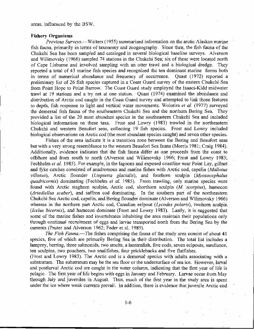
areas, influenced by the BSW.

Fishery· Organisms Previous Surveys.-Walters (1955) summarized information on the arctic Alaskanmarine

fish fauna, primarily in terms of taxonomy and zoogeography. Since then, the fish fauna of the Chukchi Sea has been sampled and cataloged in several biological baseline surveys. Alverson and Wilimovsky (1966) sampled 74 stations in the Chukchi Sea; six of these were located north of Cape Lisburne and involved sampling with an otter trawl and a biological dredge. They reported a total of 43 marine fish species and recognized the ten dominant marine forms both in terms of numerical abundance and frequency of occurrence. Quast (1972) reported a preliminary list of 26 fish species captured in a Coast Guard survey of the eastern Chukchi Sea from Point Hope to Point Barrow. The Coast Guard study employed the Isaacs-Kidd midwater trawl at 19 stations and a try net at one station.. Quast (1974) examined the abundance and distribution of Arctic cod caught in the Coast Guard survey and attempted to link those features to depth, fish response to light and vertical water movements. Wolotira et a!. (1977) surveyed the demersal fish fauna of the southeastern Chukchi Sea and the northern Bering Sea. They.· provided a list of the 20 most abundant species in the southeastern Chukchi Sea and included bIological information on these taxa. Frost and Lowry (1983) trawled in the northeastern Chukchi and western Beaufort seas, collecting 19 fish species. Frost and Lowry included· biological observations on Arctic cod (the most abundant species caught) and seven other species.

Fishes of the area indicate it is a transition zone between the Bering and Beaufort seas but with a very strong resemblance to the western Beaufort Sea fauna (Morris 1981; Craig 1984). Additionally, evidence indicates that the fish fauna differ as one proceeds from the coast to offshore and from· south to north (Alverson and Wilimovsky 1966; Frost and Lowry 1983; Fechhelm eta!' 1985). For example, in the lagoons and exposed coastline near Point Lay, gillnet and fyke catches consisted of anadromous and marine fishes with Arctic cod, capelin (Mallotus villosus), Arctic flounder (Liopsetta glacialis) , and fourhorn sculpin (Myoxocephalus quadricornis) dominating (Fechhelm et aL 1985). From trawling, only marine species were found with Arctic staghorn sculpin, Arctic cod, shorthorn sculpin (M scorpius), hamecon (Artediellus scaber), and saffron cod dominating. In the southern part of the northeastern Chukchi Sea Arctic cod, capel in, and Bering flounder dominate (Alverson and Wilimovsky 1966) whereas in the northern part Arctic cod, Canadian eelpout (Lycodes polaris), twohorn sculpin (Icelus bicornis), and hamecon dominate (Frost and Lowry 1983). Lastly, it is suggested that some of the marine fishes and invertebrates inhabiting the area maintain their populations only through continual recruitment of eggs and larvae transported north from the Bering Sea by the currents (Pruter and Alverson 1962; Feder et al. 1989).

The Fish Fauna.-The fishes comprising the fauna of the study area consist of about 41 species, five of which are primarily Bering Sea in their distribution. The total list includes a . lamprey, herring, three salmonids, two smelts, a lanternfish, five cods, seven eelpouts, sandlance, ten sculpins, two poachers, two snailfishes, four pricklebacks and five flatfishes. (Frost and Lowry 1983). The Arctic cod is a demersal species with adults associating with a substratum. The substratum may be the sea floor or the undersurface of sea ice. However, larval and postlarval Arctic cod are caught in the water column, indicating that the first year of life is pelagic. The first year of life begins with eggs in January and February.. Larvae occur from May through July and juveniles in August. Thus, much of the first year in the study area is spent under the ice where weak currents prevail. In addition, there is evidence that juvenile Arctic cod

1-6

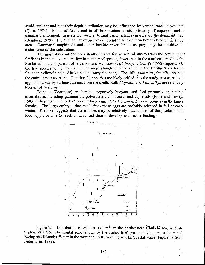
avoid sunlight and that their depth distribution may be influenced by vertical water movement (Quast 1974). Foods of Arctic cod in offshore waters consist primarily of copepods and a garnrnarid arnphipod. In nearshore waters (behind barrier islands) mysids are the "dominant prey (Bendock, 1979). The availability of prey may depend to an extent on bottom type in the study area. Garnrnarid arnphipods and other benthic invertebrates as prey may be sensitive to disturbance of the substratum.

The most abundant and consistently present fish in several surveys was the Arctic codar flatfishes in the study area are few in number of species, fewer than in the southeastern Chukchi Sea based on a comparison of Alverson and Wilimovsky's (1966)and Quast's (1972) reports. Of the five species found, four are much more abundant to the south in the Bering Sea (Bering flounder, yellowfin sole, Alaska plaice, starry flounder). The fifth, Liopsetta glacialis, inhabits the entire Arctic coastline. The first four species are likely drifted into the study area as pelagic eggs and larvae by surface currents from the south. Both Liopsetta and Platichthys are relatively tolerant of fresh water. '.

Eelpouts (Zoarcidae) are benthic, negatively buoyant, and feed primarily on benthic invertebrates including garnrnarids, polychaetes, cumaceans and caprellids (Frost and Lowry, 1983). These fish tend to develop very large eggs (2.7 - 4.5 nun in Lycodes polaris) in the larger females. The large embryos that result from these eggs are probably released in fall or early winter. The size suggests that these fishes may be relatively independent of the plankton as a food supply or able to reach an advanced state of development before feeding,

CHUKCHI SEA

7J ­

72 ­!

;9

,

['58 ,

ALASKA

I ['"i " "I ••

~ co ~ ~ '0 ~ ~ ~ ~ ~ ~

,< :g t,; ." '-l n'" ""

Figure 2a. Distribution of biomass (gC/m2) in the northeastern Chukchi sea, August­September 1986. The frontal zone (shown by the dashed line) presumably' separates the mixed' Bering shelf/Anadyr Water in the west and north from the Alaska Coastal water (Figure 68 from Feder et al. 1989).

1-7

"

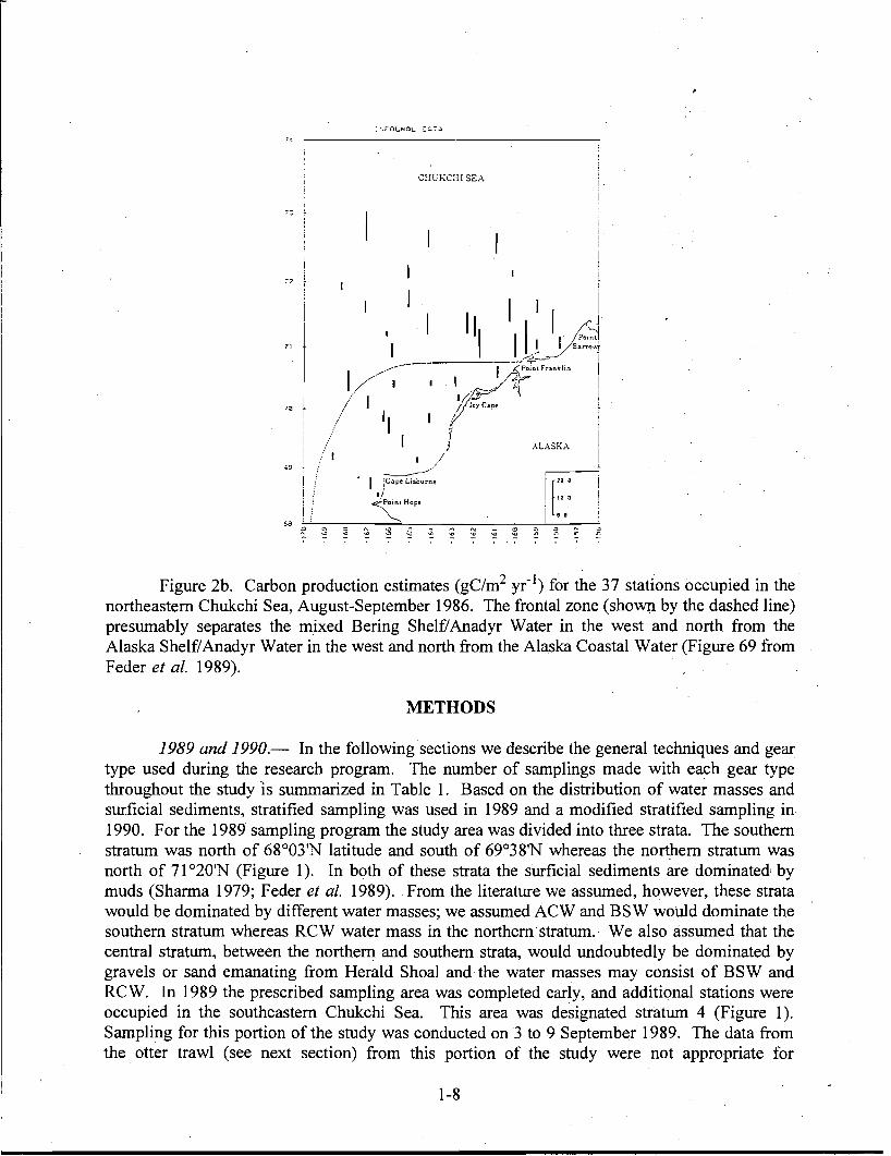
CHL'KCHI SEA

i II I II I 71 t,

1

1_L)I I1.//---;-- I _ ,1.,rFn'F".oklin

. I (,I :;:/ "'-\7. t / I ! krC'.'

I ./... 'I !" I r

j ALASKA I,.' I /

'9 - ~

i ' . I ie.p. Lisbu... [' ".

i, f ~oiRlHope1/ ' .f'" ;a ,:-,'i_'::---::--__"-----..:>......, ,-1 ..

~ ~ '"~ ~ ;2 .~

~ N

~ Sl .~ ~ f,. , ."" '" '" '"

lFigure 2b. Carbon production estimates (gC/m2 yr- ) for the 37 stations occupied in the northeastern Chukchi Sea, August-September 1986. The frontal zone (shown by the dashed line) presumably separates the mixed Bering Shelf/Anadyr Water in the west and north from the Alaska Shelf/Anadyr Water in the west and north from the Alaska Coastal Water (Figure 69 from Feder et al. 1989).

METHODS

1989 and 1990.- In the following sections we describe the general techniques and gear type used during the research program. The number of samplings made with each gear type throughout the study IS summarized in Table 1. Based on the distribution of water masses and surficial sediments, stratified sampling was used in 1989 and a modified stratified sampling in 1990. For the 1989 sampling program the study area was divided into three strata. The southern stratum was north of 68°03'N latitude and south of 69°38'N whereas the northern stratum was north of71 °20'N (Figure 1). In both of these strata the surficial sediments are dominated, by muds (Sharma 1979; Feder et al. 1989).. From the literature we assumed, however, these strata would be dominated by different water masses; we assumed ACW and BSW would dominate the southern stratum whereas RCW water mass in the northern· stratum.· We also assumed that the central stratum, between the northern and southern strata, would undoubtedly be dominated by gravels or sand emanating from Herald Shoal and the water masses may consist of BSW and RCW. In 1989 the prescribed sampling area was completed early, and additional stations were occupied in the southeastern Chukchi Sea. This area was designated stratum 4 (Figure 1). Sampling for this portion of the study was conducted on 3. to 9 September 1989. The data from the otter trawl (see next section) from this portion of the study were not appropriate for

1-8

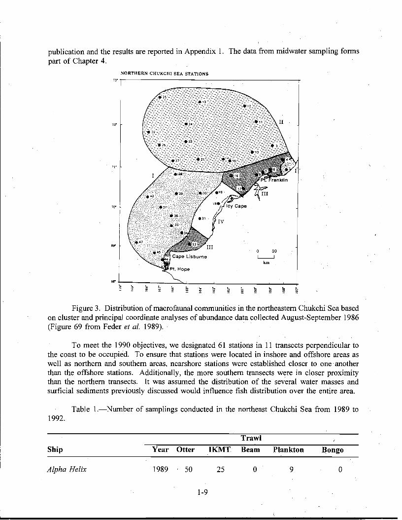
publication and the results are reported in Appendix 1. The data from midwater sampling forms part of Chapter 4.

NORTHERN CHUKCHI SEA STATIONS

7)' I

77:"

70' L

89"

88"

~ ~ ~ 0'" ~ .. ~ ": ~ !::~ ~ ~ ~'" '"

Figure 3. Distribution of macrofauna1communities in the northeastern Chukchi Sea based on cluster and principal coordinate analyses of abundance data collected August-September 1986 (Figure 69 from Feder et al. 1989). .

To meet the 1990 objectives, we designated 61 stations in 11 transects perpendicular to the coast to be occupied. To ensure that stations were located in inshore and offshore areas as well as northern and southern areas, nearshore stations were established closer to one another than the offshore stations. Additionally, the more southern transects were in closer proximity than the northern transects. It was assumed the distribution of the several water masses and surficial sediments previously discussed would influence fish distribution over the entire area.

Table I.-Number of samplings conducted in the northeast Chukchi Sea from 1989 to 1992.

Trawl

Ship Year Otter IKMT Beam Plankton Bongo

Alpha Helix 1989 \ 50 25 o 9 o

1-9

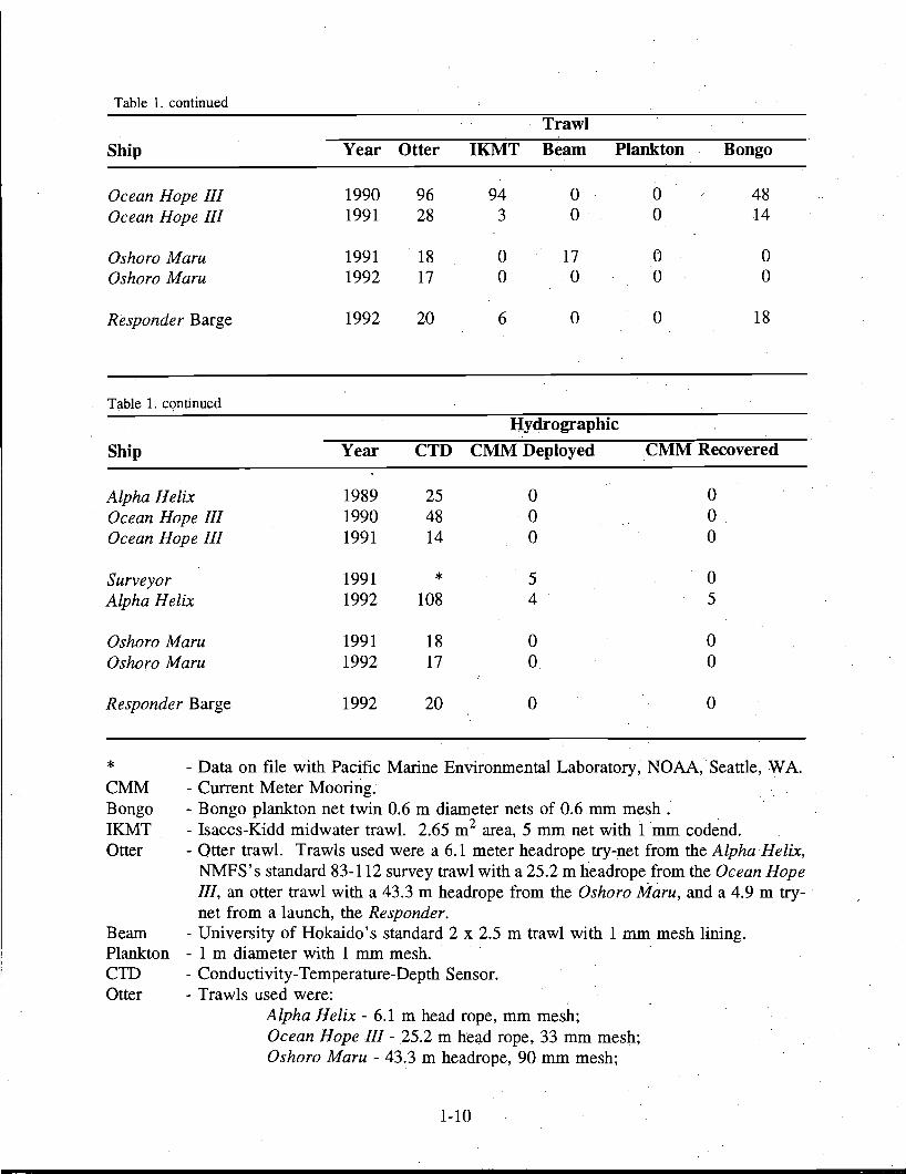
Table I. continued

Trawl

Ship Year Otter IKMT Beam Plankton Bongo

Ocean Hope III 1990 96 ·94 0 0 48 Ocean Hope III 1991 28 3 o· 0 14

Oshoro Maru 1991 18 0 17 0 0 Oshoro Maru 1992 17 0 0 0 0

Responder Barge 1992 20 6 0 0 18

Table 1. c(;mtinued

Hydrographic

Ship Year CTD CMM Deployed CMM Recovered

Alpha Helix 1989 25 0 0 Ocean Hope III 1990 48 0 0 Ocean Hope III 1991 14 0 0

Surveyor 1991 * 5 0 Alpha Helix 1992 108 4 5

Oshoro Maru 1991 18 0 0 Oshoro Maru 1992 17 0 0

Responder Barge 1992 20 0 0

* - Data on file with Pacific Marine Environmental Laboratory, NOAA, Seattle, WA. CMM - Current Meter Mooring. Bongo - Bongo plankton net twin 0.6 m diameter nets of 0.6nim mesh: IKMT - Isaccs-Kidd midwater trawl. 2.65 m2 area, 5 mm net with Imm codend. Otter - Qtter trawl. Trawls used were a 6.1 meter headrope try-net from the Alpha Helix;

NMFS's standard 83-112 survey trawl with a 25.2 m headrope from the Ocean Hope III, an otter trawl with a 43.3m headrope from the Oshoro Maru, and a 4.9 m try­net from a launch, the Responder.

Beam - University of Hokaido's standard 2 x 2.5 m trawl with 1 mm mesh lining. Plankton - 1 m diameter with 1 mm mesh. cm - Conductivity-Temperature-Depth Sensor. Otter - Trawls used were:

Alpha Helix - 6.1 m head rope, mm mesh; Ocean Hope III - 25.2 m head rope, 33 mm mesh; Oshoro Maru - 43.3 m headrope, 90 mm mesh; .

1-10

Responder - 4.9 m headrope, 5 mm mesh

This would result in fish associations differing along north to south and onshore to offshore axes. Because of the inclement weather, however, only 48 stations were occupied between 16 August and 16 September 1990 (Figure 1). Weather conditions dictated the general areas in: which we could sample and stations were numbered to reflect the sampling sequence. The data from the 1990 sampling formed the core information for many chapters in this report.

. Biological.-At each station demersal and midwater tray.rling, as well as zooplankton and Global Positioning System (GPS); LORAN C could not be used for navigation due to· radio propagation characteristics and the placement of the master and slave stations (Johnson 1989). In 1989 demersal fish were sampled from the University of Alaska's research vessel with a 6.1 m headrope otter trawl with 35 mm stretch meshed codend. At each station two one-half-hour otter trawls were conducted at speeds of approximately 2.5 kts. Fish were sorted to lowest taxonomic category possible and counted. Young-of-the-year (yay) fishes and larvae were sampled with· and Isaccs-Kidd midwater trawl (IKMT) and bongo net (see· following for description). Physical oceanographic sampling were· conducted. Each station location was determined with a

In 1990 otter trawling was conducted from a chartered fishing vessel with the National Marine Fisheries Service's (NMFS) standard 83-112 survey trawl; it had a 25.2 m head rofe and 34.1 m footrope set back 7.1cm from a tickler chain. Fish density and' biomass/km were determined by the area swept method; we noted the boat's location when the net reached bottom and when the trawl left the bottom upon its retrieval. Additionally, the width of the wings and height of the headrope above the footrope were determined with a Scanmar mensuration unit. Upon the net's retrieval the entire catch was weighed in the net with an electronic load cell (4,536 kg capacity), fish were sorted to the lowest taxonomic category possible, counted, placed in baskets, and weighed with a mechanical platform scale (81.6 kg capacity). Total length measurements and otoliths were obtained from subsamples of Arctic cod,. Bering flounder, Myoxocephalus cf. verrucosa, and Lycodes raridens. Total lengths were determined with a measuring board to the nearest centimeter, and both sagittal otoliths excised and stored in vials containing a solution of 50:50 glycerin:water containing thymol (Chilton and Beamish, ·1982). Subsamples of Arctic staghorn sculpin were frozen and returned to the laboratory where standard and total lengths were determined to the nearest millimeter withdividers and weight determined to the nearest 0.01 g on an electric pan balance. They were then sexed, ovaries weighed and preserved in vials containing Gilson's solution (Bagenal and Braum, 1978), otoliths obtained and stored as previously described, and stomachs stored iIi vials of 70% ethanol. Weights were obtained to the nearest 0.01 gram. Trawl-caught invertebrates were also identified to the lowest taxonomic categories possible and weighed. Certain species, for example snow crab and Neptunia spp., were also counted and weighed.

Midwater fishes were sampled with an IKMT having a 1.8 m head bar (sampling a 2.65 m2 area), 5 mm mesh net, and a collecting bucket with a 1mm mesh screen. In the net's mouth a flowmeter was attached to determine water volume sampled. The IKMT was towed obliquely, the wire let out until it was estimated to be several meters al;lOve the bottom and then pulled in at about 1 m/sec as the boat traveled at approximately 2-2.5 kts. Ichthyop1ankton was sampled with a bongo net having 60 cm diameter openings (110 cm2 area) and 1 mm mesh netting in which a flow meter was suspended. The bucket screens were also of 1 mm mesh netting~ Samples were preserved in 5% formaldehyde solution, returned to the laboratory, and sorted. Juveniles and larvae were separated from both the IKMT and bongo net samples, and stored in

. 1-11

a buffered 5% formaldehyde solution. Juveniles were identified following Baxter (unpublished manuscript, Annotated Key to the Fishes ofAlaska), and counted. With the aid of a dissecting microscope, ichthyoplankton were identified following Matarese et al. (1989), and counted. Abundance was expressed as numbers/ 1000 m3. The volume sampled was determined framthe area of the IKMT and bongo nets openings and the revolutions of the flow meters (calibrated as to the revolutions/distance traveled).

. Ages were estimated by examination of the external surface of otoliths and burnt otolith sections (Barber and McFarlane, 1987). Surface aging was done by. placing each whole, unground otolith in a watchglass of glycerin:water solution and examining each under reflected light with a dark background through a dissecting microscope.· A number of otoliths for each . species were examined and criteria for annuli developed prior to aging each fish. Age estimates were obtained twice, followed by a third examination for those which did not agree. Mter ages were estimated from the surface, for those which were large enough, one otolith from each fish was randomly chosen and broken as near as possible through the nucleus and· burned in an alcohol flame. Under a dissecting microscope the burned surface was brushed lightly with vegetable oil and examined under reflected light Again, criteria for an annulus were developed prior to aging the fish. A true age validation study has not been conducted on any of the species involved in this study and will be very difficult to do so. Alternatively we collected fins from a subsample of Arctic cod and Arctic staghorn sculpin and attempted to obtain age information from these structures. The finrays proved to be to small and inappropriate for aging.

A hierarchical cluster analysis of fish collected at each station sampled in the 1990 and . 1991 sampling was performed following Feder et at. (1989). In this case, the mean number of . each species collected from the two trawls at each station was used to calculate the Czekanowski coefficient and used to calculate the similarity matrices for the stations. The results of these analyses are presented in Chapter 9.

Physical.-Vertical profiles of temperature and salinity were made at each station with a Seabird SBE 19 internally recording CTD (conductivity-temperature-depth) instrument. Because of a malfunction in the internal memory of the CTD, however, data from only 45 of the 52 CTD casts were recovered. At most stations calibration samples were collected for salinity and temperature with a Niskin bottle equipped with a reversing thermometer. The salinity samples were analyzed after the cruise with an Autosal laboratory salinometer. The results of the 1989 cruise are reported in Appendix 1 and data from the 1990 and 1991 ichthyofauna sampling is supporting information for Chapters 2, 4,7, and 9.

1991 and 1992 Biological.-In 1991 biological sampling was again conducted from a chartered fishing

vesseL Additionally, "Ships of opportunity" were also utilized. The University of Hokkaido's research vessel Oshoro Maru was used to collect information on snow crab and ichthyop1allkton. Additionally, a pilot program was initiated where sampling with the bongo net, IKMT,and a try net was attempted from a launch offloaded from a barge used as a support vessel for the oil drill ship.

Because all stations were not occupied in 1990, additional sampling was conducted from 14 - 25 September 1991 from a chartered trawler. Eight stations established in 1990 were reoccupied in 1991 and an additional eight stations were established and sampled (Figure 1; locations are listed in Table 2 of Chapter 5). Techniques used in sampling during 1991 were identical to those previously described. The purpose was to gain wider coverage, estimate interannual variability of abundance, biomass, and species, and to collect reproductive data on

1-12

snow crab (Chapter 11): Sampling was conducted from Oshoro Maru on 25July to 31 August 1991 (Figure 1) and

1992. In 1991 fishes and snow crab, for reproductive information, were collected with an otter trawl having a 43.3 m headrope and 48.6 m footrope fitted with rollers, and a 90 mm codend mesh. YOY and larval fishes were sampled with the University of Hokkaido's standard beam trawl with a 2 x 2.5 m square mouth and a net 17 m long with mesh grading from 65 mm to a 4 mm; the codend had a 1 mm lining. ' In- 1992 sampling was conducted as in the previous year; however, the otter trawl had a 45 mm mesh liner in the cod-end. Information on snow crab obtained during the cruise will be found in Chapter 11 and on ichthyoplankton in Chapter 4, and fishes collected listed in Appendix 4.

A pilot program was initiated in 1991 where sampling was conducted in the vicinity of the drill ship (located at 71°20'N l65°25.8'W) from a 10.9 m launch deployed from the barge, Responder (a drill ship support vessel). Sampling was conducted on 24-27 July, 13 - 18 August, and 28 September 1991. The launch was equipped'with a detachable A-frame and diesel powered winch system to deploy and retrieve sampling gear. Sampling gears used were the IKMT, the . bongo net, and a 4.9 m otter trawl of 5 mm mesh netting. Additionally, CTD casts were made

,as previously described. Data from these cruises may be found in Appendix 6. Some of the information on YOY fishes and ichthyoplankton was used in Chapter 4.

The CTD data set was supplemented by year-long measurements, at hourly intervals, of ocean currents, temperature, and salinity from five current meter moorings. The moorings were deployed in collaboration with researchers from NOAA's Pacific Marine Environmental Laboratory during a cruise aboard the NOAA vessel Surveyor conducted from 22 September to 11 October 1991. The original deployment plan called for moorings to be deployed in Barrow Canyon (within the Alaska Coastal Current) and in the north central Chukchi Sea' (between Herald and Hanna Shoals). The Barrow Canyon moorings were designed to: 1) gauge flow and water mass property variations within the Alaska Coastal Current, 2) determine the frequency and on-shelf extent of water upwelled along the continental, slope, 'and 3) build upon previous observations which indicated large interannual variations in winter production of e;x.tremely saline water formed on the northeast shelf. The area between Hanna and Herald Shoal was chosen for investigation because it had been the focus of recent oil exploration activities and the prevailing circulation pattern was unknown. However, heavy ice conditions prevented the vessel from reaching two of the three planned sites in the north central Chukchi Sea; Instead, these two moorings were deployed offshore of Cape Lisburne essentially bracketing the front between ACW and BSW. In the end, this turned out to be a fortuitous choice as the circulation in the winter of 1991/92 turned out to differ significantly from previous conceptions and the data from these moorings proved crucial in determining the reasons for this circulation change.

The moorings were recovered in collaboration with researchers from Japan's Marine Science and Technology Center (JAMStEC) from a cruise aboard the University of Alaska's Alpha Helix conducted from 14 September to 9 October 1992. An extensive grid of CTD stations, covering the entire Chukchi Sea was also occupied on this cruise and the results are presented in Chapter 3.

1-13

CHAPTER 2

OCEANOGRAPHY OF THE NORTHEAST CHUKCHI SEA: A REVIEW I .•

THOMAS J. WEINGARTNER

Institute of Marine Science, University of Alaska Fairbanks Fairbanks, Alaska 99775-7220

Abstract.-This paper reviews the physical o~eanography of the ice-free season (July-October) of the northeast Chukchi Sea. This shelf sea is unique among those adjoining the Arctic Ocean because its physical and biological characteristics are profoundly influenced by the northward transport of Pacific Ocean waters through Bering Strait. A portion of this inflow, the Alaska Coastal Water, is wanned and diluted in summer by solar heating and river runoff and flows across the northeast Chukchi shelf within the Alaska Coastal Current (ACC). The dynamics of this current are governed by the large-scale pressure gradient between the Pacific and Arctic oceans, the density contrast between shelf water masses, and the local wind field. The core of the ACC parallels the bathymetry and coincides with a bottom temperature front. Current speed and frontal strength vary in proportion to the topographic relief. Surface fronts are also observed·but they are more variable and not necessarily collocated with the bottomfront. The regional oceanography is also affected by upwelling along the. shelfbreak and mixing and circulation along the seasonally varying ice-edge. Accumulating evidence reveals very large interannual variability in winds, sea-ice extent, and the northward transport through Bering Strait; all of which contribute to the environmental variability of the Chukchi Sea.

INTRODUCTION

The Chukchi Sea lies at the northeastern end of the enonnous Eurasian continental shelf system of the Arctic Ocean. These shelf seas (Barents, Kara, Laptev, East Siberian, and Chukchi Seas) comprise 12% of the continental shelf area of the globe (2.6 x 107 km2, Walsh [1988]) and 22% of the total area of the Arctic Ocean (17 x 106 km2, Carmack [1990]). The Chukchi Sea is unique among arctic shelf seas in that waters of Pacific Ocean origin flow across it and exert a profound influence on its circulation, the sea-ice, and water properties.

This paper reviews the physical oceanographic characteristics of the northeast Chukchi Sea. The open water season (mid-July through October) is emphasized because it is of primary concern to fisheries biologists and relatively little data have been collected during the ice-covered seasons. The northeast shelf is highlighted because it has been the focus of recent research spurred by concerns related to oil exploration activities. Moreover, due to limited access to the western Chukchi Sea, little infonnation has been published on this region since the monograph by Coachman et al. (1975). More, detailed infonnation on the oceanography of the Bering Strait and southern Chukchi Sea are found in Coachma,n et ai. (1975) and Walsh et al.(1989).

The plan of the paper is as follows. The next section describes the bathymetry of the

ISubmitted for publication in Fish Ecology in Arctic North America.

2-1

region and this is followed by a description of the seasonl:l1 variation in the wind field. Both the bathymetry and the winds strongly influence the mean flow field of which the gross features are described in the section entitled "Chukchi Sea Circulation". The various ~ater masses of the Chukchi Sea, which are mainly of advective origin rather than a consequence of in-situ formation, are then presented. With these four sections as background, the section entitled "Hydrography and Circulation of the northeast Chukchi Sea" provides specific examples of both and shows how they are interrelated. Aspects of shelfbreak upwelling and its implications for the Chukchi Sea are discussed in the "Upwelling" section. The "Sea-ice"sectiori describes the seasonal distribution of sea-ice and aspects of ice-edge oceanography; AccuQlulating evidence indicates that the Chukchi Sea is subject to large interannual variations and examples of this variability are described in the "Interannual Variability" section. The finll.l section of the paper concludes with a summary. Figure 1 illustrates the bathymetry and provides a reference map for the place names used throughout the text.

BATHYMETRY

The Chukchi Sea is bounded to the north by the shelfbreak (~200 m isobath) of the Arctic Ocean and to the south by Bering Strait - a distance of more than 800 km (Figure 1). Its lateral extent varies from a minimum of about 85 km in Bering Strait to a maximum of about 900 km between Long Strait in the west and Pt. Barrow in the east.

The basin has a relatively flat bottom, with depths deepening gradually from 30 m in the east to 55 m in the west. There are, however, several important bathymetric features which steer the currents and influence sea-ice and water property distributions: 1) Hope Sea Valley, a broad 55 m deep depression, extending northwest from the southern Chukchi Sea to Herald Sea Valley, 2) Herald Shoal in the center of the basin and, 3) Hanna Shoal in the northeast. The latter two have minimum depths of about 25 m.

. Two shelfbreak bathymetric features facilitate cross-shelf exchange of water. by steering currents and by channeling upwelled water onto the shelf: 1) Herald Sea Valley, east of Wrangel Island, is a relatively gentle, 50 km wide depression which terminates on the shelf at about 150 m depth, and 2) Barrow Canyon, a steep-sided canyon originating offshore of Pt. Franklin, cuts across the continental slope, and terminates a~ depths greater than 3000 m. Both canyons are the main conduits through which shelf water enters the Arctic Ocean (Coachman et ai. 1975). Shelfbreak isobaths diverge from east to west such that bottom slopes decrease from 10 mIkin in the northeast to 1 m/km in the northwest Chukchi Sea. This bathym~tric change might have implications for the exchange of shelf waters with those of the Arctic Ocean (see Upwelling).

WINDS

Wind stress acting directly on the surface of the ·ocean or coupled to the ocean via a floating ice pack accelerates ocean currents. For shallow seas,such as the Chukchi, winds are important because they can induce rapid changes in the current structure over the whole water column and, consequently, redistribute water mass properties.

Winds over the Chukchi and northern Bering seas are strongly influenced by a polar high pressure cell centered at about 79~, 1700 W (Pease 1987). On average, this pressure system drives easterly winds over the northern Chukchi Sea and northeasterly winds over the southern Chukchi and northern Bering Seas. North of Point Lay (~69.5~), the monthly mean winds vary little throughout the year and the variance about these monthly means is constant from February

2-2

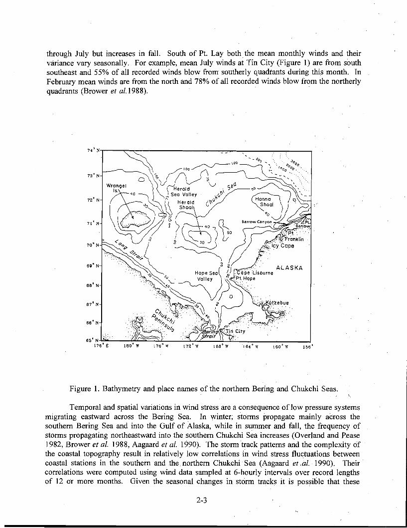
through July but increases in fall. South of Pt. Lay both the mean monthly winds and their variance vary seasonally. For example, mean July winds at Tin City (Figure 1) are from south southeast and 55% of all recorded winds blow from southerly quadrants during this month. In February mean winds are from the north and 78% of all recorded winds blow from the northerly quadrants (Brower et al. 1988).

74' N..,-~~~----------::--=----:----~_...,.... __...,

73' N

72' N

71' N

70' N

69' N

68' N

67' N

66' N

\00

"0 ~100~\I/~V-~v a

~:r?/~" . " Se'" Sea Valley' ,+-v'r­" Herald G'r-v

Shoal

. ',::Pt::' . " :. ....:....:.:.:...::rranklin

:"\ Icy Cope

ALASKA

65' N~i;;.;.;.,.-~~::S::::::~:""-_~~L=~~~ ..J 176' E 160' 11 176' W 172'·W 160' W

Figure 1. Bathymetry and place names of the northern Bering and Chukchi Seas.

Temporal and spatial variations in wind stress are a consequence of low pressure systems migrating eastward across the Bering Sea. In winter; stcmns propagate mainly across the southern Bering Sea and into the Gulf of Alaska, while in summer and fall, the frequency of storms propagating northeastward into the southern Chukchi Sea increases (Overland and Pease 1982, Brower et al. 1988, Aagaard et al. 1990). The storm track patterns and the complexity of the coastal topography result in relatively low correlations in wind stress fluctuations between coastal stations in the southern and the. northern Chukchi' Sea (Aagaard et .al.·· 1990). Their correlations were computed using wind data sampled at 6-hourly intervals over record lengths of 12 ot more months. Given the seasonal changes in storm tracks it is possible that these'

. .

2-3

correlations also vary seasonally such that the spatial correlation of the winds is greater in winter than in the summenand fall. Spatial heterogeneity of the wind field. in autumn influences the current structure of the northeast Chukchi Sea; south winds in the southern Chukchi Sea accelerate coastal currents northward whereas north winds in the northeast Chukchi Sea accelerate coastal currents southward. Differential advection of distinct water masses by these currents could establish strong horizontal gradients (fronts) in temperature and salinity.,

CHUKCHI SEA CIRCULATION

The most important circulation feature of the Chukchi Sea is the northward flow through Bering Strait which has a mean annual transport of 0.'8 Sv (Coachman and Aagaard 1988; 1 Sverdrup = 106 m3/s). This transport is driven by the 0.5 meter drop in sea level between the Pacific Ocean and the Arctic Ocean (Overland and Roach 1987). Approximately 85% of this inflow originates in the deep Bering Sea and the Gulf of Anadyr (Kinder et al. 1986) with the remainder derived from the northeast Bering shelf. Transport fluctuations, at time scales which range from days to weeks, are of the same'magnitude as the mean and are correlated with the north-south winds (Coachman and Aagaard 1988). Northward transport is minimum in winter when north winds prevail and is maximum in summer when south winds occur more frequently.

The Bering Strait throughflow bifurcates offshore of Lisburne Peninsula; one branch continues along the northeast coast as the Alaska Coastal Current (ACC) and the remainder flows to the northwest. Both of these flows are sustained, in part, by the sea-level difference between the Bering Sea and Arctic Ocean. The northwestward current consists of a diffuse, slowly drifting transport through the Hope and Herald Sea valleys (Coachman et al. 1975). In contrast, the ACC is a swift (0.2 mls) coastal current whose main axis is. found within 20 - 50 Ian of the Alaskan coast and which flows into the Arctic Ocean through Barrow Canyon. There is also a southeastward flow, the Siberian Coastal Current, which enters the Chukchi Sea through Long Strait and flows along the Chukotsk Peninsula before commingling with the Bering Strait inflow.

Relatively little is known about the circulation over the shelfbreak of the northern Chukchi Sea. However, hydrography (reviewed by Carmack 1990) and trajectories of buoys deployed in sea-ice (Colony 1984) indicate that, on average, currents in the upper 50 m flow westward and comprise the southern limb of the wind-driven anticyclonic (clockwise) gyry of the Arctic Ocean (Coachman and Aagaard 1974). Beneath this surface layer and extending to at least 2500 m . depth, hydrography and moored current meter observations collected along the continental slope of the Alaskan Beaufort Sea (Aagaard 1984, Aagaard et al. 1990) reveal a well-defined eastward flow, the Beaufort Undercurrent, which flows opposite to the prevailing east winds. This current has a width of about 70 Ian and appears to be a persistent feature of the Arctic Ocean's' circulation. Between 60 and 100 m depth mean speeds are about .05 mls but fluctuations up to 1 mls are common. Above 250 m depth, its source waters originate in the Bering Sea and drainage from Eurasian shelves. 'Beneath 250 m depth, undercurrent waters originate in the Atlantic Ocean which enter the eastern Arctic Ocean through Fram Strait in the Greenland Sea.. Presumably the undercurrent is weaker to the west of the Chukchi Sea because of the decrease in shelfbreak slope (cf. Bathymetry) and because its volume increases after the Bering Strait inflow has joined it. While the dynamics of this undercurrent await theoretical study, they must be related, in part, to these inflows. Insofar as the undercurrent flows in a direction opposite to that of the wind, with shallow water to its right, it bears a strong similarity to the poleward flowing undercurrents along the eastern boundaries of mid-latitude oceans and it is probable that these undercurrents share similar dynamics. '

2-4

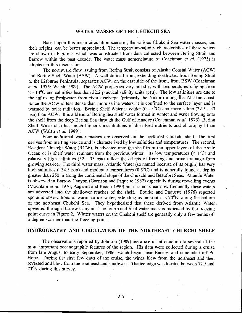
WATER MASSES OF THE CHUKCHI SEA

Based upon this mean circulation scenario, the various Chukchi Sea water masses, and their origins, can be better appreciated. The temperature-salinity characteristics of these waters are shown in Figure 2 which was constructed from data collected between Bering Strait and Barrow within the past decade. The water mass nomenclature of Coachman et al. (1975) is adopted in this discussion.

The northward flow issuing from Bering Strait consists of Alaska Coastal Water (ACW) and Bering Shelf Water (BSW). A well-defined front, extending northward from Bering Strait to.the Lisburne Peninsula, separates ACW, on the east side of the front, from BSW (Coachman et al. 1975; Walsh 1989). The ACW properties vary broadly, with temperatures ranging from 2 - 13°C and salinities less than 32.2 practical salinity units (psu). The low salinities are due to the influx of freshwater from river discharge (primarily the Yukon) along iheAlaskan coast. Since the ACW is less dense than more saline waters, it is confined to the surface layer and is warmed by solar radiation. Bering Shelf Water is colder (0 - 3°C) and more saline (32.5 - 33 psu) than ACW. It is a blend of Bering Sea shelf water formed in winter and water flowing onto the shelf from the deep Bering Sea through the Gulf of Anadyr (Coachman et al. 1975). Bering Shelf Water also has much higher concentrations of dissolved nutrients and chlorophyll than ACW (Walsh et al. 1989).

Four additional water masses are observed on the northeast Chukchi shelf. The first derives from melting sea-ice and is characterized by low salinities and temperatures. The second, Resident Chukchi Water (RCW), is advected onto the shelf from the upper layers of the Arctic Ocean or is shelf water remnant from the previous winter. Its low temperatures « 1°C) and relatively high salinities (32 - 33 psu) reflect the effects of freezing and brine drainage from growing sea-ice. The third water mass, Atlantic Water (so named because of its origin) has very high salinities (-34.5 psu) and moderate temperatures (0.5°C) andis generally f~und at depths greater than 250 m along the continental slope of the Chukchi and Beaufort Seas. Atlantic Water is observed in Barrow Canyon (Garrison and Paquette 1982) especially during upwelling events (Mountain et al. 1976; Aagaard and Roach 1990) but it is not clear how frequently these waters are advected into the shallower reaches of the shelf. . Bourke and Paquette (1976) reported sporadic observations of warm, saline water, extending as far south as 70~, along the bottom of the northeast Chukchi Sea. They hypothesized that these derived from Atlantic Water. upwelled through Barrow Canyon. The fourth and final water mass is indicated by the freezing point curve in Figure 2. Winter waters on the Chukchi shelf are generally only a few tenths of a degree warmer than the freezing point.

HYDROGRAPHY AND CIRCULATION OF THE NORTHEAST CHUKCHI SHELF

The observations reported by Johnson (1989) are a useful introduction to several of the more important oceanographic features of the region. His data were collected during a cruise from late August to early September, 1986, which began near Barrow and concluded off Pt. Hope. During the first few days of the cruise, the winds blew from the northeast and then reversed and blew from the southeast and southwest. The ice-edge was located between 72.5 and 73~ during this survey.

2-5 .

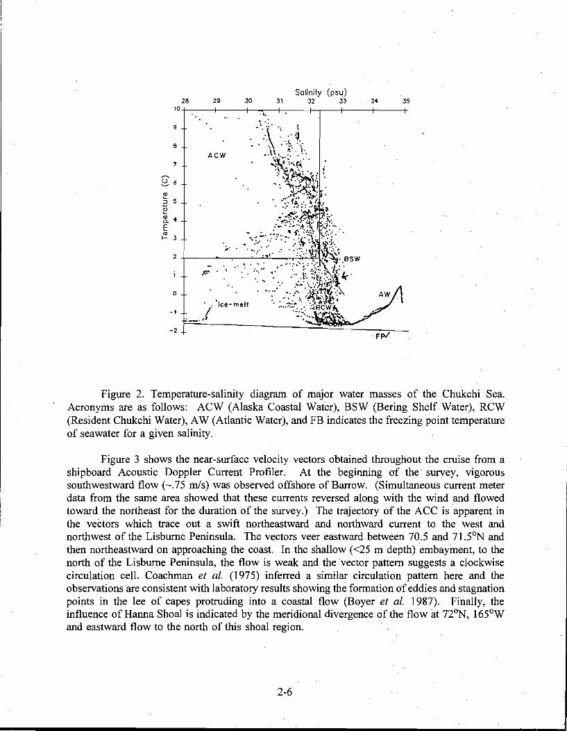
Salinity (psu) 26 29 30 31 32 33 34 35

.,.

.' ~ -. .': .. " . .' . "

Ice-melt

oFp/ ..

10

9

6 ACW

7

,.... 85 ~

5.3 0 ~

~ 4 E Ql

I- 3

2

.fJ'

0

-1 ._.i.-

,

-2

Figure 2. Temperature-salinity diagram of major water masses of the Chukchi Sea. Acronyms are as follows: ACW (Alaska Coastal Water), BSW (Bering. Shelf Water), RCW (Resident Chukchi Water), AW (Atlantic Water), and FB indicates the freezing point temperature of seawater for a given salinity.

Figure 3 shows the near-surface velocity vectors obtained throughout the cruise from a shipboard Acoustic Doppler Current Profiler. At the beginning of the survey, vigorous southwestward flow (~.75 m/s) was observed offshore of Barrow. (Simultaneous current meter data from the same area showed that these currents reversed along with the wind and flowed toward the northeast for the duration of the survey.) The trajectory of the ACC is apparent in the vectors which trace out a swift northeastward and northward current to the west and northwest of the Lisburne Peninsula. The vectors veer eastward between 70.5 and 71.5~ and then northeastward on approaching the coast. In the shallow «25 m depth) embayment, to the north of the Lisburne Peninsula, the flow is weak and the vector pattern suggests a clockwise circulation cell. Coachman et al. (1975) inferred a similar circulation pattern here and the observations are consistent with laboratory results showing the formation ofeddies and stagnation points in the lee of capes protruding into a coastal flow (Boyer et al. 1987). Finally, the influence of Hanna Shoal is indicated by the meridional divergence of the flow·at 72~, 165°W and eastward flow to the north of this shoal region.

2-6

------

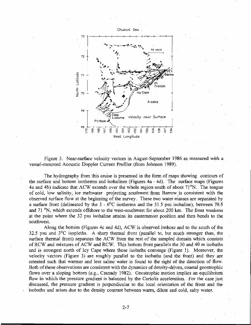
Chukchi Sea

73 i--+--+---+---+---+-I--+---+--+--+--+-'+-----i-----t

72

V "'0 71

:E o -l

..r:::. ~ ..... o 70 Z

69

Velocity near Surface Pt Hope

68 +--+---+----+---+-'>-f-I--+-'--+---+----+---+---+-----'t---+ a (J) aJ ,..... (0 ~ ~ n N _ 0 m ~ ,..... w ,..... (0 W <0 (0 (0 (0 (0 W W W ~ ~ ~ ~

West. Longitude

Figure 3. Near-surface velocity vectors in August-September 1986 as measured with a . vessel-mounted Acoustic Doppler Current Profiler (from Johnson 1989).

The hydrography from this cruise is presented in the form of maps showing contours of the surface and bottom isotherms and isohalines (Figures 4a - 4d). The surface maps (Figures 4a and 4b) indicate that ACW extends over the whole region south of about 71~. The tongue of cold, low salinity, ice meltwater projecting southwest from Barrow is consistent with the observed surface flow at the beginning of the survey. These two water masses are separated by a surface front (delineated by the 3 - 6°C isotherms and the 31.5 psuisohaline), between 70.5 and 71 ~, which extends offshore to the west-southwest for about 200 kIn. The front weakens at the point where the 32 psu isohaline attains its easternmost position and then bends to the southwest.

Along the bottom (Figures 4c and 4d), ACW. is observed inshore and to the south of the 32.5 psu and 3°C isopleths. A sharp thermal front (parallel to, but much stronger than, the surface thermal front) separates the ACW from the rest of the sampled domain which consists of RCW and mixtures of ACW and RCW. This bottom front parallels the 30 and 40 m isobaths and is strongest north of Icy Cape where these isobaths converge (Figure 1).. Moreover, the velocity vectors (Figure 3) are roughly parallel to the isobaths (and the front) and they are oriented such that warmer and less saline water is found to the right of the direction of flow.. Both of these observations are consistent with the dynamics ofdensity-driven, coastal geostrophic flows over a sloping bottom (e.g., Csanady 1982). Geostrophic motion implies an equilibrium flow in which the pressure gradient is balanced by the Coriolis acceleration. For the case just discussed, the pressure gradient is perpendicular to the local orientation of the front and the isobaths and arises due to the density contrast between warm, dilute and cold, salty water.

2-7

••

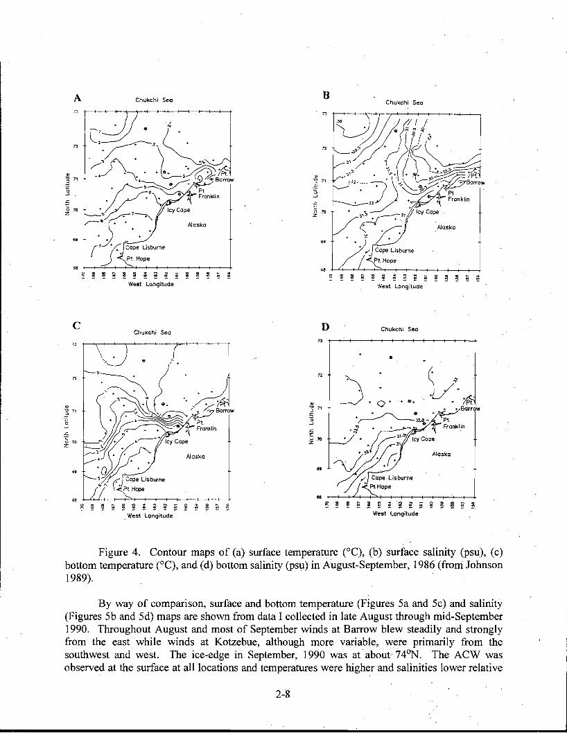
c

BA Chukchi Sea Chukchi Sea

~ ~ N ~i2 ~ ~ ~ .. ;: :;l .. g ~ ~ ~ ~

~ ~

~ ~ West Longitude West Longitude

D Chukchi SeaChukchi Sea

T.l1--"";""'--+--+--+--+--+--+--+-+--+-->--+---t ­

e

o~· (', •. n

(J"~~~..'\\.~ r e•.",'~ •. 3 " 711 (~~~.' Barrow

n

."" 71

.3

3 =e o 70 Z

59

5. 0

. .,. 4~. ~:~nldin ....~ .'-- Icy Cape ~ .W;>tt

7:1", + + Alaska. . ·0 ..:~~m.~

\..; Pt Hope

:g -' .t: t w '" Z

.

l/·.• .Pt"

+ + Barrow Q + .~ $.

~ ~~ ~ ~ ~ West LongitudeWest Longitude..

Figure 4.. Contour maps of (a) surface temperature (DC), (b) surface s~linity (psu), (c) bottom temperature (DC), and (d) bottom salinity (psu) in August-September, 1986 (froni Johnson 1989).

By way of comparison, surface and bottom temperature (Figures 5a and 5c) and salinitY (Figures 5b and 5d) maps are shown from data I collected in late Augustthrough mid-September 1990. Throughout August and most of September winds at Barrow blew steadily and strongly from the east while winds at Kotzebue, although more variable, were primarily from the southwest and west. The ice-edge in September, 1990 was atabout 74~. The ACW was observed at the surface at all locations and temperatures were higher and salinities lower relative

~ N ~ ~.. .. .. .. .. g ., .. ! ! ! ~ ! ~ ~ .~ ~ ~ ~ ~ ~ ~ ;! !

2-8

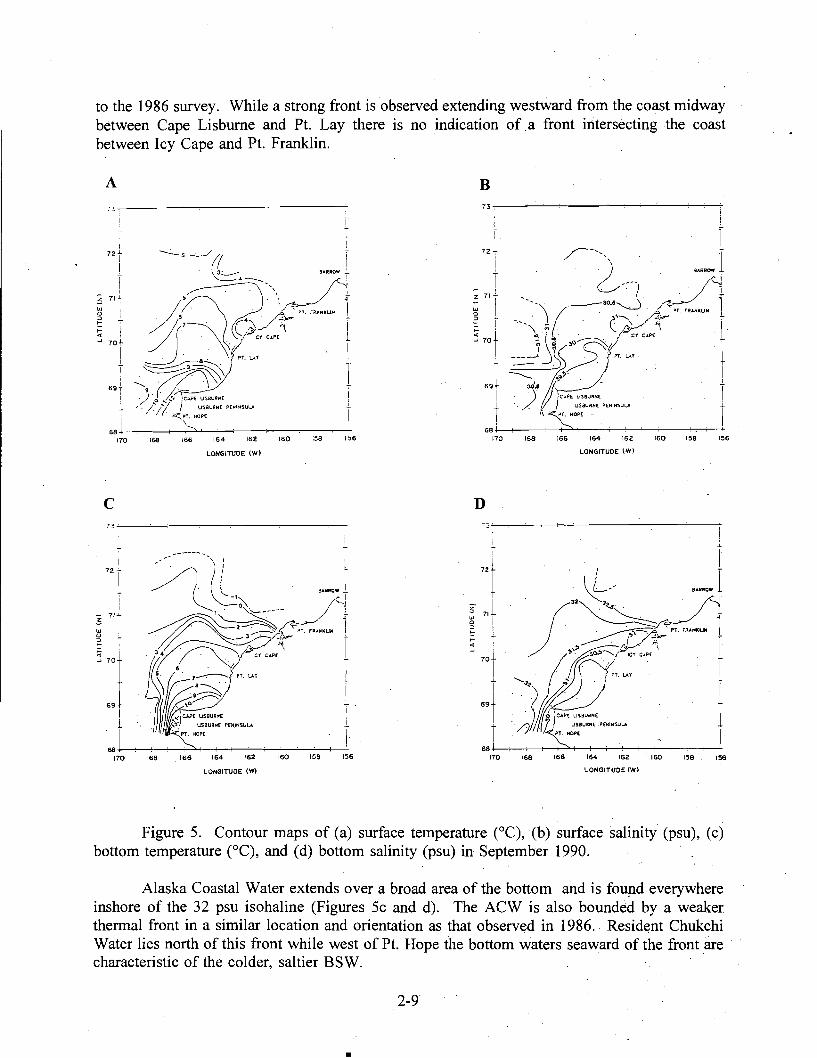
c

to the 1986 survey. While a strong front is observed extending westward from the coast midway between Cape Lisburne and Pt. Lay there is no indication of a front intersecting the coast between Icy Cape and Pt. Franklin.

A B .~~.---~~-----------:-

~5~~ ! ;l~AOW ~

T .•~-\ -.-/~

"\ A' -X:.."..~ I 70t

I

t.~~ I ~69+ ----.

I '/ ',0 /."r~BUAH( i ~'. / /1. J USaUAN[ P(,..IN~Ul..A

.,.!

.l...

set . . ,:$-:OPE. • I 1701GB 166 164 162 160 :58 156

LONGITUOE (W)

,i

-"I, ,

~-L-.) -~ rl--V-....~~· 1 ~ 70t- _ " \" ~ ';,,,- ' 1

1 UT--.1~~?':b ?T. 1 i ~ ~~'}. I

69~ 30.5 1 I ) jeAPE US8UA~( I 1. USaUAI'l( PENINSULA 1

69 +.-1 1~~\:S:----+-""","HO+-PE_'~,~--+---+-_-+ .....,...~

170 168 166 164 162 160 158 156

LONGITUDE IWI

D

170 168 . 166 164 162 160 "159 156

LONGITUDE (WI

. .

Figure 5. Contour maps of (a) surface temperature (OC),(b) surface salinity (psu), (c) bottom temperature (OC), and (d) bottom salinity (psu) in September 1990.

Alaska Coastal Water extends over a broad area of the bottom and is found everywhere inshore of the 32 psu isohaline (Figures 5c and d). The ACW is also bounded by a weaker thermal front in a similar location and orientation as that observed in 1986. Resident Chukchi Water lies north of this front while west of Pt. Hope the bottom waters seaward of the front are characteristic of the colder, saltier BSW. .. .

2-9

..

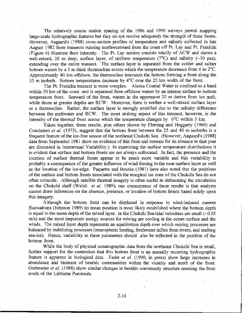
The relatively coarse station spacing of the 1986 and 1990 surveys pennit mapping large-scale hydrographic features but they do not resolve adequately the strength of these fronts. However, Aagaard's (1988) cross-section profiles of temperature and salinity collected in late August 1982 from transects running northwestward from the coast off Pt. Lay and Pt. Franklin (Figure 6) illustrate their intensity.. The Pt. Lay section consists wholly of ACW and shows a well-mixed, 20 m deep, surface layer, of unifonn temperature (7°C) and salinity (~30 psu), extending over the entire transect. The surface layer is separated from the colder and saltier bottom waters by a 5 m thick thennoc1ine across which the temperature decreases from 6 to 2°C. Approximately 40 km offshore, the thennoc1ine intersects the bottom fonning a front along the 35 m isobath. Bottom temperatures decrease by 4°C over the 25, km width of the front.

The Pt. Franklin transect is more complex. Alaska Coastal Water is confined to a band within 20 km of the coast and is separated from offshore waters by an intense surface to bottom temperature front. Seaward of the front, waters in the uppennost 20 m derive from ice melt, while those at greater depths are RCW. Moreover, there is neither a well-mixed surface layer or a thennoc1ine. Rather, the surface layer is strongly stratified due to the salinity difference' between the meltwater and RCW. The most striking aspect of this transect, however, is the intensity of the thennal front across which the temperature changes by 6°C within 5 km.

Taken together, these results, plus others shown by Fleming and Heggarty (1966) and Coachman et al. (1975), suggest that the bottom front between the 25 and 40 m isobaths is a frequent feature of the ice-free season of the northeast Chukchi Sea. (However, Aagaard's [1988] data from September 1981 show no evidence of this front and reasons for its absence in that year are discussed in Interannual Variability.) In examining the surface temperature distributions it is evident that surface and bottom fronts are not always collocated. In fact, the presence and the location of surface thennal fronts appear to be much more variable and this variability is probably a consequence of the greater influence of wind forcing in the near-surface layer aswell as the location of the ice-edge.. Paquette and Bourke (1981) have also noted that the positions of the surface and bottom fronts associated with the marginal ice zone of the Chukchi Sea do not often coincide. Although satellite thennal imagery is often useful in delineating the circulation on the Chukchi shelf (Walsh et al. 1989), one consequence of these results is that analysts cannot draw inferences on the absence, presence, or location of bottom fronts based solely upon

. this imagery. Although the bottom front can be displaced in response to wind-induced current

fluctuations (Johnson 1989) its mean position is most likely established where the bottom depth is equal to the mean depth of the mixed layer. In the Chukchi Sea tidal velocities are small (~O.05

mfs) and the most important energy sources for mixing are cooling at the ocean surface and the winds. The mixed layer depth represents an equilibrium depth over which mixing processes are balanced by stabilizing processes (atmospheric heating, freshwater influx fromrivers, and melting sea-ice). Hence, variability in these parameters should also be reflected in the position of the bottom front.

While the body of physical oceanographic data from the' northeast Chukchi Sea is small, further support for the contention that this bottom front is an annually recurring hydrographic feature is apparent in biological data. Feder et al. (1990; in press) show large increases in abundance and biomass of benthic communities within the vicinity and north of the front. Grebmeier et al. (1988) show similar changes in benthic community structure crossing the front south of the Lisburne Peninsula.

2-10

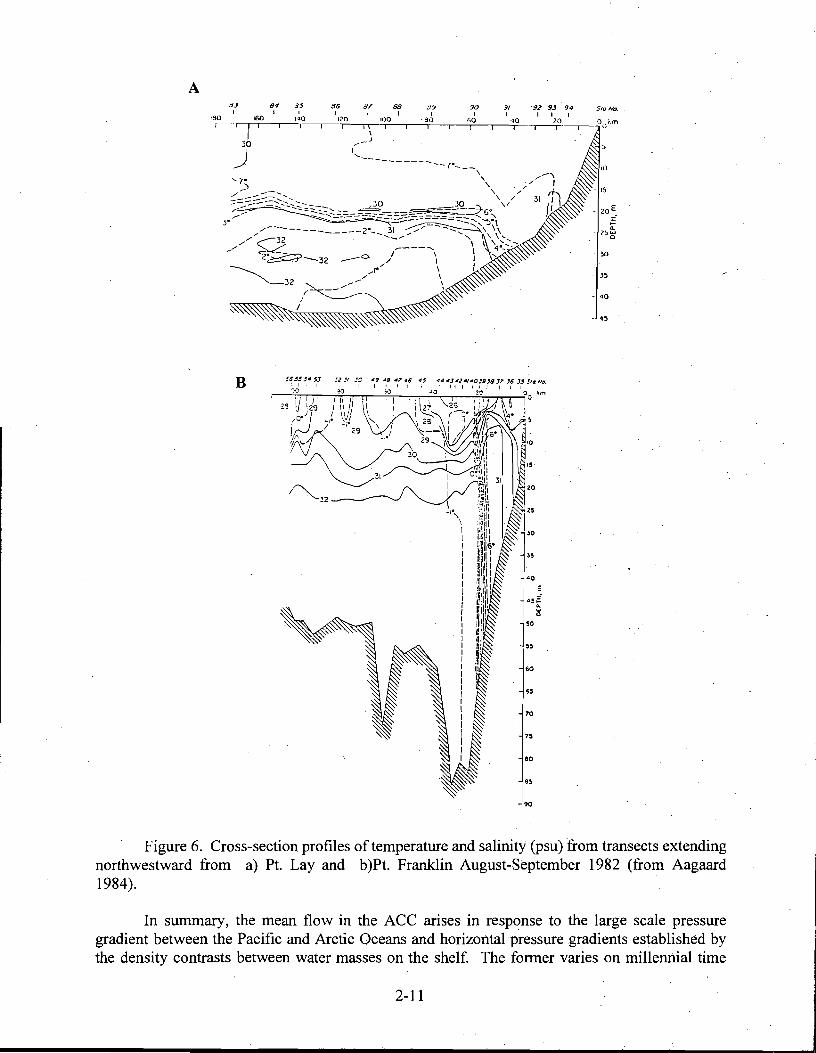
A d.J 84 85 86 87 88 8!1 90 9/ ·92 93 94 5fo No.

I I I I I I I I I I I I tBO 160 140 120 100 80 60 ~o 20 0 Jo.m ~I~~"'-'--'----'l': '-----,---.TI'---.---TI--,------r"-----.- ()

30 ,,_Jj (,

-30

- J~

- _0

- .~

B

Figure 6. Cross-section profiles of temperature and salinity (psu) from transects extending northwestward from a) Pt. Lay and b)Pt. Franklin August-September 1982 (from Aagaard 1984).

In summary, the mean flow in the ACC arises in response to the large scale pressure gradient between the Pacific and Arctic Oceans and horizontal pressure gradients established by the density contrasts between water masses on the shelf. The former varies on millennial time

2-11

scales while the latter varies seasonally and in response to synoptic atmospheric pressure patterns. The main axis of this current is parallel to a bottom front oriented along the bathymetry. Along the current's axis, speeds vary in conjunction with the strength, of the front and the magnitude of the bottom slope. The latter point is illustrated by the mean and maximum current speeds reported by Aagaard (1988) from year-long cUiTent meter records obtained offshore of Pt. Franklin (large bottom slope) and Cape Lisburne (smaller bottom slope). Mean and maximum speeds from the Pt. Franklin moorings were 0.2 mls and 1.1 mis, respectively. The corresponding values for the Cape Lisburne moorings were 0.05 mls and 0.62 mls.

Johnson's (1989) and Aagaard's (1988) results show that superpos~d on the mean flow of the ACC are large temporal variations, which occur on time scales of days to weeks, and which are correlated with the north-south wind component. (Northward winds accelerate the along-isobath flow component, i.e., in the same direction as the mean flow. Southward winds decelerate this flow component and sufficiently strong southward winds can lead lo current reversals.) This current variability might play an important role in transporting shelf water into the interior of the western Arctic Ocean given D'Asaro's (1988) hypothesis that, at the mouth of Barrow Canyon, these fluctuations generate the long-lived eddies observed throughout the interior of the western Arctic Ocean. Aagaard's (1988) results show that along-isobath current fluctuations at the Pt. Franklin moorings were also correlated with· those at Cape Lisburne implying that the velocity field' of the northeast Chukchi Sea is coherent over alongshore distances as large as 350 km. The current response to fluctuations in the wind field occurs rapidly «1 day) and, within the vicinity of the front, is accompanied by dramatic temperature and salinity changes (Johnson 1989). Such effects can complicate the interpretation of hydrographic data collected over a large area during a two to three week cruise and indicate the need to consider the wind history of this region in analyzing such data.

UPWELLING

The deeper (-100 m depth) waters offshore of the shelfbreak of the northern Chukchi Sea provide a potentially important source of nutrient rich water for this shelf.. At still greater depths (-250 m), waters upwelled from the Atlantic layer could exert a substantial change in the

. temperature-salinity structure of, the. northern Chukchi Sea as· well as provide nutrients. Shelfbreak upwelling provides a mechanism for the flux of these waters onto the shelf. Episodic upwelling in Barrow Canyon and along the shelfbreak of the Beaufort Sea is a frequent phenomenon which has been inferred from hydrographic data (Garrison and Paquette 1982; Bourke and Paquette 1976; Hufford 1974) and observed in current meter records (Mountain et al. 1976 and Aagaard and Roach 1990) from the same area, Aagaard and Roach's (1990) results show that upwelling, from depths as great as 300 m, occurred along the Alaskan Beaufort Sea shelfbreak in the form of eastward propagating events of about five days duration. While these I.

upwellings were not well-correlated with local winds they were most common in fall and early. winter when winds were most variable. They suggest that these episodes are a response of the shelfbreak circulation to large-scale stochastic wind forcing and theoretical support for this hypothesis is implied by the numerical model results of Philander and Yoon (1982).

Once upwelled the deeper waters will influence the shelf if they can be advected shoreward. Data from Aagaard and Roach's (1990) mooring anchored on the 150 m isobath within Barrow Canyon suggest that average upcanyon (onshore) velocities during upwelling episodes were about .25 mls. Over the five-day duration of such an event, water parcels would be displaced 125 km upcanyon or as far inshore as the 60 m isobath. In contrast, their current

2-12

records from the Beaufort Sea shelfbreak show that upwelling-related onshore velocities were much smaller than those observed in Barrow Canyon. This is not unexpected given that onshore flow is weaker over regions of large bottom slope (i.e., the Beaufort shelfbreak) than over regions of gentle bottom slope (Johnson and Rockliff 1986). Hence, the westward decrease in slope. along the Chukchi Sea shelfbreak suggests that the· onshore excursion of upwelled water here might be greater than in the Beaufort Sea. This hypothesis remains untested because, to date, no long-term measurements have been made on this part ofthe shelfbreak..

SEA-ICE

The Chukchi Sea is generally ice-covered from November through' June. North of Bering Strait, the seasonal retreat of sea-ice begins in June and, in the mean, attains its farthest north position along about 72.S~ in mid-September (Naval Oceanography Command Detachment 1986). In comparison to the Beaufort and East Siberian Seas, ice-retreat begins earlier and . ice-advance occurs later on the· Chukchi shelf due to the influence of warm water advected northward through Bering Strait. However, interannual differences in the seasonal retreat, advance, and position of the ice-edge are related to the winds (Muench et al. 1991; e.g., north winds advect the ice-edge southward and vice-versa). .

The northward retreat of the ice-edge during the summer months does not proceed uniformly along its length. Figure 7 (from Muench 1990) shows that the ice-edge between Wrangel Island and Pt. Barrow is markedly indented by three "me~tback embayments" whose relative positions vary little from year-to-year. Two of these embayments overlie Herald Sea Valley and Barrow Canyon and the third is observed between Herald and Hanna shoals.. All are related to bathymetric steering of the northward flow of warm waters. (The data of Paquette and Bourke [1981] clearly show the northward advection of warm water between Herald and Hanna shoals and this flow is also suggested by spreading of the bottom isotherms at about 71~,

16SoW in Figures 4c and Sc.) These "meltback embayments" might have biological significance because there are marked differences between the wind-forced circulation along a straight ice-edge and a meandering ice-edge. The model of Roed and O'Brien (1983) shows that for a straight ice-edge, zonally oriented such that open water lies to the south of the ice, winds from the east result in upwelling along the ice-edge and winds from the west result in downwelling. Hakkinen's (1986) model results show that if an ice-edge has meanders (i.e., embayments) . upwelling occurs on the windward side of the meander and downwelling on the lee side. High rates of primary production are often associated with ice-edges (Niebauer199l) and ice-edge. upwelling of nutrients would enhance this productivity. In the northern Chukchi Sea, where mean winds are from the east and vary primarily in the zonal direction, these embayments could be significant sites for carbon fixation. Hakkinen's (1986) model results further imply that biological production along the ice-edge of the Chukchi Sea could vary dramatically in both time and space and that field programs must be suitably designed to address this issue.

2-13

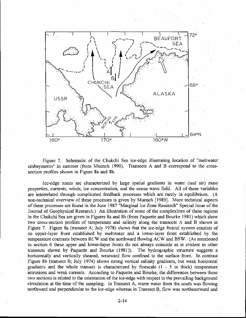
BEAUFORT SEA

ALASKA

--- .......( \. \ -- ......) -_ ..... '"

.: -::. ':: ':. . :

~ ..

f, I \

I \ I \ \ \ I \

I ' ­ ....

I ~,-) ..... 1 Al

BICHUKCHI

~ USSR

L-....l.. ­ ....l..-.........""""""__....l..-__----"'--...L.­ ...L.­ ....I.....,;,.....I 64°N

Figure 7. Schematic of the Chukchi Sea ice-edge illustrating location of "meltwater embayments" in summer (from Muench 1990). Transects A and B correspond to the cross­section profiles shown in Figure 8a and 8b.

Ice-edge zones are characterized by large spatial gradients in water (and air) mass properties, currents, winds, ice concentration, and the ocean wave field. All of these variables are interrelated through complicated feedback processes which are rarely in' equilibrium. (A non-technical overview of these processes is given by Muench [1989]. More technical aspects of these processes are found in the June 1987 "Marginal Ice Zone Research" Special Issue of the Journal of Geophysical Research.) An illustration of some of the complexities of these regions' in the Chukchi Sea are given in Figures 8a and 8b (from Paquette and Bourke 1981) which show two cross-section profiles of temperature and salinity along the transects A and B shown in Figure 7. Figure 8a (transect A; July 1978) shows that the ice-edge frontal system consists of . an upper-layer front established by meltwater and a lower-layer front established by' the temperature contrasts between RCW and the northwm:d flowing ACW and BSW. (As mentioned in section 6 these upper and lower-layer fronts do not always coincide as is evident in other transects shown by Paquette and Bourke (1981)). The hydrographic structure suggests a horizontally and vertically sheared, westward flow confined to the surface front. In contrast Figure 8b (transect B; July 1974) shows strong vertical salinity gradients, but weak horizontal gradients and the whole transect is characterized by finescale (1 - 5 m thick) temperature intrusions and weak currents. According to Paquette and Bourke, the, differences between these . two sections is related to the orientation of the ice-edge with respect to the prevailing background circulation at the time of the sampling. In Transect A, warm water from the, south was flowing northward and perpendicular to the ice-edge whereas in Transect B, flow was northeastward and

2-14

..

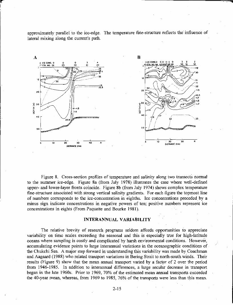
approximately parallel to the ice-edge. The temperature fine-structure reflects the influence of lateral mixing along the current's path.

A B

·····3'

o ICE CONe. D 2~ STA. NO. 24

,.---- ­ __-1.6 ... 32.~

~O

30 . o

40

-I.~

·····.33u ,

10f::;::=;=~~'

20

~[ 1·I'~~S 10 20 30 40 N S 10 20 30

DISTANCE (Km) N

DISTANCE IKml

Figure 8. Cross-section profiles of temperature and salinity along two transects normal to the summer ice-edge. Figure 8a (from July 1978) illustrates the case where well-defined upper- and lower-layer fronts coincide.. Figure 8b (from July 1974) shows complex temperature fine-structure associated with strong vertical salinity gradients. For each figure the topmost line of numbers corresponds to the ice-concentration in eighths. Ice concentrations preceded by a minus sign indicate concentrations in negative powers of ten; positive numbers represent ice concentrations in eights (From Paquette and Bourke 1981).

INTERANNUAL VARIABILITY

The relative brevity of research programs seldom affords opportunities to appreciate variability on time scales exceeding the seasonal and this is especially true for high-latitude oceans where sampling is costly and complicated by harsh environmental conditions. However, accumulating evidence points to large interannual variations in the oceanographic conditions of .. the Chukchi Sea. A major step forward in understanding this variability was made by Coachman

.and Aagaard (1988) who related transport variations in Bering Strait to north-south winds. Their results (Figure 9) show that the mean annual transport varied by a factor of 2 over the period from 1946-1985. In addition to interannual differences, a large secular decrease in transport began in the late 1960s. Prior to 1969, 70% of the estimated mean annual transports exceeded the 40-year mean, whereas, from 1969 to 1985, 76% of tht:: transports were less than this mean.

2-15

Such variations should have important consequences for the Chukchi Sea because of the implied variation in the northward flux of heat, salt, and nutrients, but few data exist· upon _which conclusions regarding the effect of this variability can be made. However, in the section on upwelling it was noted that Aagaard's (1988) data from September 1981 showed no indication of the bottom front which was argued to be a frequent feature of the northeast Chukchi Sea; The absence of this front in 1981 is seen in the cross-section profiles of temperature and salinity .' along the Pt. Lay transect shown in Figure 10 (the corresponding transect for 1982 was shown in Figure 6a). Moreover, no ACW is present along this transect which consists of very cold (~-1 DC) RCW along the bottom and within 80 km of the .coast and meltwater elsewhere. Differences between the 1981 hydrography and the years discussed' previously could be associated with differences in winds. Figure 11 shows time series of the monthly anomaly of the north-south surface wind component at 67.5~, 167.5°W for the period 1981 to 1991. (The monthly anomalies are the deviates from the mean wind for that month.. The wind components are estimated from synoptic atmospheric pressure grids following Aagaard et al. [1990].) Time series of this variable to the south and north of this location are quite similar. The data show persistent, north wind anomalies from July through November 1981. In 1986 and 1990 south . wind anomalies prevailed during these months while in 1982 both north' and south anomalies were observed. The magnitude and persistence of the 1981 wind anomalies would have resulted in: 1) reduced northward transport through Bering Strait thereby increasing the time required to flush winter water from the Chukchi shelf, and 2) westward displacement of ACW from the northeast Chukchi Sea.

Coachman and Shigaev (1992) have also documented temperature and salinity (and, by implication, other constituents) differences in the source waters feeding into Bering Strait.' They show that these waters were most saline in the late 1960's and least saline in the mid-1970's. Temperatures and salinities of southeastern Bering Shelfwater also show considerable interannual variations and these are associated with interannual variability in ice cover over the Bering Sea shelf such that cold, dilute bottom waters in summer follow extensive winter ice cover, and vice versa.

Summer-fall sea-ice extent in the Chukchi Sea also varies enormously from year-to-year. For example, the Naval Oceanography Command Detachment (1986) atlas shows that the mid-September ice-edge position in the northern Chukchi Sea ranges from 70 to 75~ - a distance of over 500 km. Mysak et al. (1990) analyzed variations in sea-ice extent over the Chukchi and Beaufort Seas for the period 1953 to 1985 and show that interannual differences can ~ount to nearly 300% and that these differences can persist for from three to six years. They argue that the variability is related to variations in regional winds and coastal freshwater discharge induced by hemispheric-scale atmospheric fluctuations.

SUMMARY

The preceding sections have shown that the bathymetry, meteorology, sea-ice distribution, and northward advection of waters through Bering Strait profoundly influence the oceanography of the northeast Chukchi Sea. One of the more important hydrographic features observed during the open water season is the frequent occurrence of a bottom thermal front which parallels the bathymetry and the core of the Alaska Coastal Current. Biologically, the front appears to be an important feeding area for marine mammals preying on benthic organisms and a "boundary" across which benthic and fish community structure change markedly (Feder et al. 1990; Feder et al. in press; Wylie-Echeverria et al. in this volume; Smith et al. in this volume).

2-16

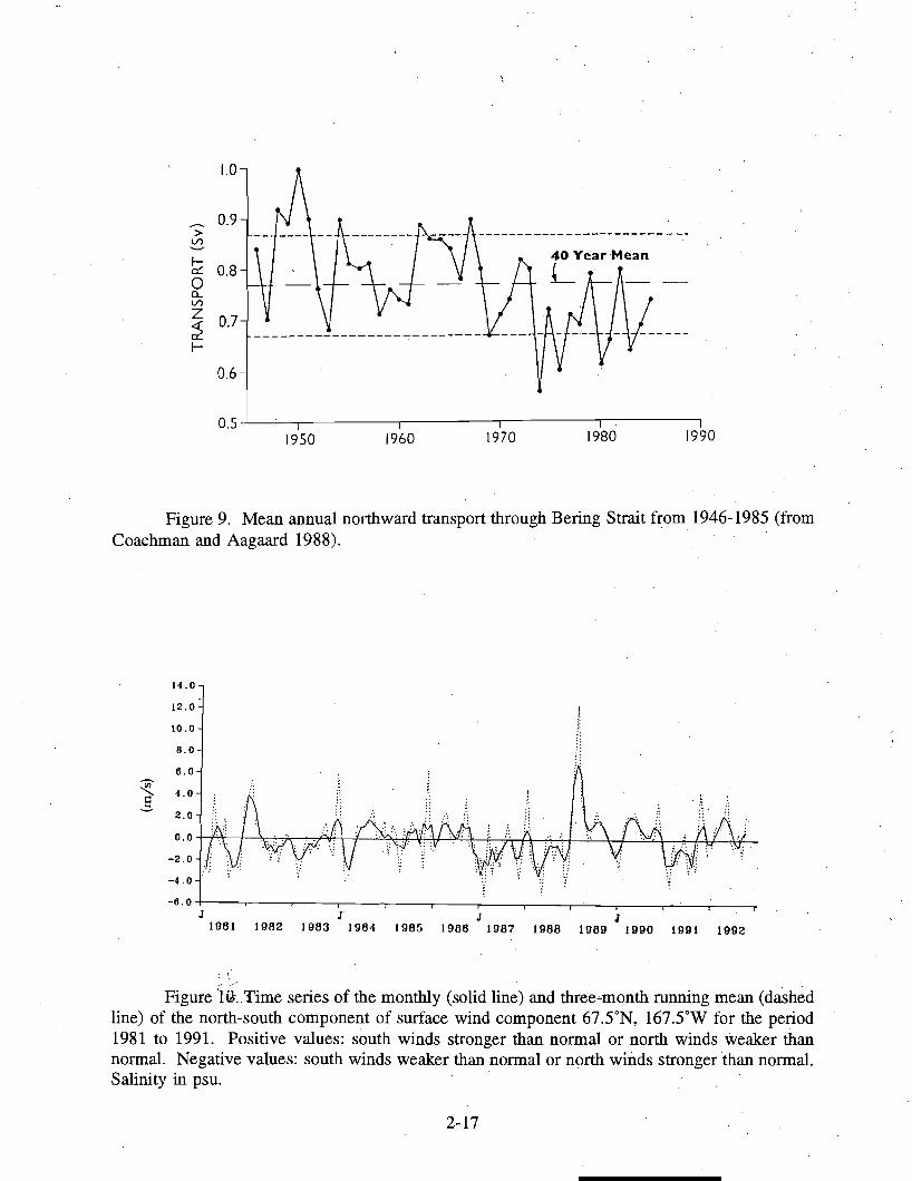
1.0

.---.. 0.9 >

Vl--­~ 0.8 0 0­Vl

z 0.7 ~ f ­

0.6

0.5 1950 1960 1970 1980 1990

Figure 9. Mean annual northward transport through Bering Strait from 1946~1985 (from Coachman and Aagaard 1988).

14.0

12.0

10.0

8.0

6.0

~ 4.0g 2.0

0.0

-2.0

-4.0

-6.0

J J J 1982 1983 1984 1985 1988 1987 1988 1989 1990 199 I 1992

Figure lIiLTime series of the monthly (solid line) and three~month running mean (dashed line) of the north-south component of surface wind component 67.5°N, 167.5°W for the period 1981 to 1991. Positive values: south winds stronger than normal or north winds weaker than normal. Negative values: south winds weaker than normal or north winds stronger than normal. Salinity in psu.

2-17

J 1981

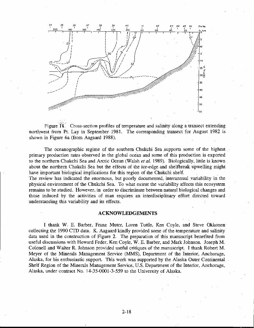
3'1 35 36 37 38 I I 1 1 I

200 180 160 140

I 1 I

29

~) -:..-- ­ 0·

~~---J

'1\ ./

/' /

I I I I I I

39 t

120

42 1

60

43 44 45 46 Slo.No. 1 I I I

40 20

20

- 25 E X t­n.

30'"Cl

35

40

I 45

/~ •

50

55

Figure';l~l-: Cross-section profiles of temperature and salinity along a transect extending northwest from Pt. Lay in September 1981. The corresponding transect for August 1982 is shown in Figure 6a (from Aagaard 1988).

The oceanographic regime of the southern chukchi Sea supports some of the highest.· primary production rates observed in the global ocean and some of this production is exported to the northern Chukchi Sea and Arctic Ocean (Walsh et at. 1989). Biologically, little is known. about the northern Chukchi Sea but the effects of the ice-edge and shelfbreak upwelling might have important biological implications for this region of the Chukchi shelf. The review has indicated the enormous, but poorly documented, interannual variability in the physical environment of the Chukchi Sea. To what extent the variability affects this ecosystem remains to be studied. However, in order to discriminate between natural biological changes and those induced by the activities of man requires an interdisciplinary effort. directed toward understanding this variability and its effects.

ACKNOWLEDGEMENTS

I thank W. E. Barber, Franz Muter, Loren Tuttle, Ken Coyle, and Steve Okkonen collecting the 1990 CID data. K. Aagaard kindly provided some of the temperature and salinity data used in the construction of Figure 2. The preparation of this manuscript benefited from useful discussions with Howard Feder, Ken Coyle, W. E. Barber, and Mark Johnson. Joseph M. Colonell and Walter R. Johnson provided useful critiques of the manuscript. I thank Robert M. Meyer of the Minerals Management Service (MMS), Department of the Interior, Anchorage, Alaska, for his enthusiastic support. This work was supported by the Alaska Outer Continental Shelf Region of the Minerals Management Service, U.S. DeparUnent of the Interior, Anchorage, Alaska, under contract No. 14-35-0001-3-559 to the University of Alaska.

2-18

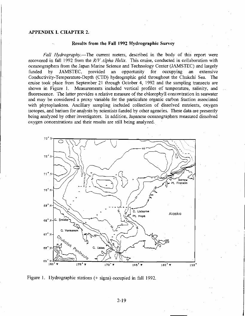
APPENDIX I. CHAPTER 2.

Results from the Fall 1992 Hydrographic Survey

Fall Hydrography.-The current meters, described in the body of this report were recovered in fall 1992 from the R/V Alpha Helix. This cruise, conducted in collaboration with oceanographers from the Japan Marine Science and Technology Center (JAMSTEC) and largely funded by JAMSTEC, provided an opportunity for occupying an extensive Conductivity-Temperature-Depth (CTD) hydrographic grid throughout the Chukchi Sea. The cruise took place from September 21 through October 4, 1992 and the sampling transects are shown in Figure 1. Measurements included vertical profiles of temperature, salinity, and fluorescence. The latter provides a relative measure of the chlorophyll concentration in se~water

and may be considered a proxy variable for the particulate organic carbon fraction associated with phytoplankton. Ancillary sampling included collection of disso1ved nutrients, oxygen isotopes, and barium for an~lysis by scientists funded by other agencies. These data are presently being analyzed by other investigators. In addition, Japanese oceanographers measured dissolved oxygen concentrations and their results are still being analyzed..

.. ".

72' Ii

71' N

70' N

89' N

Alaska

88' N

85' N~~;;;;""';;-..l..l.--:-_"""'~~",:,,"""_.I....).......:l:. ..J J80'W 175'W 170'11' 185'W 180'W. 155'

Figure 1. Hydrographic stations (+ signs) occupied in fall 1992.

2-19

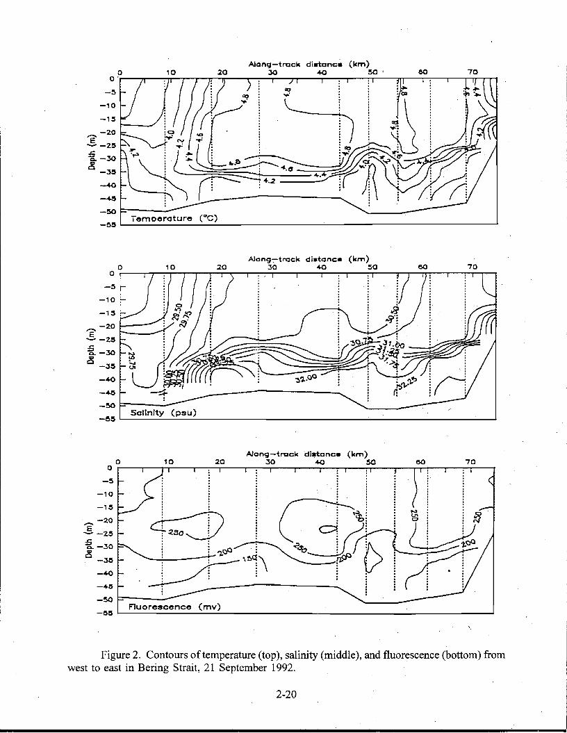
Along-track dlatanc. (km) o 10 20 .:so -4-0 50 60 70

o r---"T"""-r-r----,r---:--,--__.--;-.---r--r---"T"""---:'__.-~--r-.......,.~~__.-_:_T-___r

-5

-10 :

~ =:: ~ !.

j ~i i IS i ~

:=~: i2BO :~~oO/t~~t(~c>:~ -3l5 ~~\:>9\ p-<P.!: 1

-40 : :: :::: .: :. . i : : :

--4-e : :. : : I

: : -50l::""----­-o~ '--Fluorescence (mv) ---1

Figure 2. Contours of temperature (top), salinity (middle), and fluorescence (bottom) from west to east in Bering Strait, 21 September 1992.

2-20

The temperature and salinity observations stand in sharp contrast to results previously reported for Bering Strait. For example, Coachman et ai. (1975) and Walsh et al. (1989) find that the warmest and most dilute waters (Alaska Coastal Water, or ACW) lie at the surface on the eastern side of the strait and that the coldest and most saline waters (Anadyr Water, according to Coachman et ai. 1975) are found near the bottom on the western side of the strait. Typically there is a strong front separating these two water masses. Our interpretation of the water mass distribution on 9/21 is as follows. The cool, low-salinity waters on the western side of the strait represent a southward extension of the Siberian Coastal Current (SCC). This current flows southeastward along the north coast of the Chukotsk Peninsula, but is believed to mix with waters flowing northward through Bering Strait and then. to recirculate throughout the Chukchi Sea (Coachman et ai. 1975). In fact, these authors state that observations of SCC waters in Bering Strait are extremely rare. (It should also be remembered that because of the historical political climate access to Russian waters on the west side of Bering Strait has been very limited. Therefore, relative to the east side, relatively few measurements have been made in the western channel.) However, strong northerly winds prior to and during occupation of this transect could have forced SCC waters southward through the strait.

Fluorescence values are relatively uniform throughout this section and, as will be seen, relatively low in comparison to values obtained on other transects. Low pigment concentrations are typical of the river-fed ACW (Walsh et ai. 1989) and presumablyof the SCC as well.

Next consider the Cape Lisburne transect occupied on September 23 (Figure 3). The strong winds had abated by 9/22 and calm conditions prevailed allowing sufficient time for the coastal circulation to adjust dynamically to the new wind regime. Temperatures are relatively uniform across this section, whereas salinities are lowest adjacent to the coast arid there is a suggestion of a weak salinity front at the western stations. Shoreward of this weak front the water column consists Alaska Coastal Water (ACW).while seaward of it the water mass consists of a mixture of ACW and Bering Shelf Water (BSW). The salinity distribution implies a weak northward baroclinic flow across the whole section. Fluorescence values are several time greater than those obtained in Bering Strait and they approximately double in value proceeding seaward across the salinity front. The increase in fluorescence between the ACW water mass and the mixture of ACWand BSW is consistent with the higher particulate organic carbon carried by BSW (Walsh et al. 1989). That comparatively low fluorescence values were observed in the Bering Strait section is presumably due to the virtual absence of the BSW mass during occupation of that section.

Due to heavy ice conditions, we were able to occupy only a short transect (-25 km) extending southeast from the ice edge to near the coast near Point Franklin. This section cuts across the head of Barrow Canyon. As shown in Figure 4, conditions on this transect are considerably different from those to the south and reflect the influence of meltwater from sea-ice. Ice concentrations were greatest along the first 5 km of the transect and consisted of rotting floes as well as newly formed grease ice. Although there is considerable hydrographic complexity in this section, several features are readily discernible. First, the· narrow core of ~arin (>. 3°C) subsurface waters near the center ofthe section represents ACW flowing northeastward along the east flank of Barrow Canyon and within the core of the Alaska Coastal Current. .It is bounded to the west by the cold, saline Resident Chukchi Water (RCW). The upper 30 meters of the water column consist of ice meltwater and mixtures of this with ACW and RCW. Prominently featured in these transects are strong thermal fronts bracketing the ACW and the strong vertical stratification associated with the meltwater. The strongest stratification is observed at the westernmost station and maximum fluorescence values lie atop the pycnocline here.. Oxygen

2-21

saturation values at these stations are about 110% (Y. Sasaki and H. Ichii,personal communication) suggesting active photosynthesis by these phytoplankton. The implication of high biological production at this location is not unexpected given that enhanced primary productivity is often associated with stably stratified ice-edges (Niebauer et al. 1991). Although few primary production measurements have been made in the northeast Chukchi Sea, Feder et aI., (1993) suggest that production at the ice-edge of this region might be a significant source of carbon for the benthos of the northeast Chukchi Sea. Moreover, while ACW is impoverished with respect to nutrients (Walsh et al. 1989), sufficient concentrations are available in RCW to support primary production at this level (Feder et al. 1993).

The transect shown in Figure 5 extends across the northern Chukchi. Sea from Point Franklin in the east to Herald Sea Valley in the west. This transect runs parallel to the ice-edge and many of the stations were within 25 Ian of the ice-edge. The eastern half of the transect is well-stratified; the upper 25 m consists of a mixture of ice meltwater and ACW while beneath this layer ACW is observed. Nowhere on this section is RCW observed, indicating that winter. waters had been flushed to the north by the time this transect was occupied. Heavy concentrations of melting ice were encountered overlying Herald Shoal where stratified conditions are also observed within the upper 10m. Overlying the depression to the east of Herald- Shoal and between these two stratified regions is a narrow zone of relatively warm (> 2.00 C), salty(> 32.p psu), and unstratified water consisting of a mixture of ACW and BSW. Fluorescence values are high within this band and I believe that it represents the northward· extension of the high chlorophyll water observed along the western portion of the 9/23 occupation of the Cape Lisburne transect (see Figure 3). This zone is bracketed on either side by surface intersecting fronts. The orientation of the isohalines suggests strong northward baroclinic shear on the east side of this depression and weaker, southward baroclinic shear on the west side. The existence of strong northward flow on the east side of this depression is verified by the current meter data discussed in Chapter 3. The high fluorescence· values observed in this depression suggest that this northward flow could be a significant source of particulate organic carbon for the benthos ofthe outer shelf. Whether or not the southward flow on the west is a pennanent circulation feature associated with cyclonic flow around Herald Shoal, as suggested by Coachman. et at. (1975), or a transitory circulation feature associated with the ice-edge cannot be addressed with this data set.

To the west of Herald Shoal and over the eastern slope of Herald Canyon is a second band of unstratified, relatively warm and saline water characteristic of BSW.. It is bounded on the west by a strong ice-edge front overlying the center of Herald Canyon. Baroclinic flow along the ice-edge front is to the south, while along the east side of the canyon it is to the north. Fluorescence values are a maximum within the northward flowing BSW and decay rapidly on crossing through the ice-edge front.

Figure 6 shows the distribution of properties along the transect running from south to north along the axis of Herald Canyon. The section is characterized by a subsurface temperature maximum (indicated by the 2.5 °C isothenn) with an associated maxima in fluorescence. Surface waters consist of ice meltwater and mixtures of meltwater with BSW.Cold, saline RCW is observed at the north end of the transect and beneath 40 m depth. The data imply northward flow through Herald Canyon of BSW which carries a substantial particulate organic carbon load.

2-22

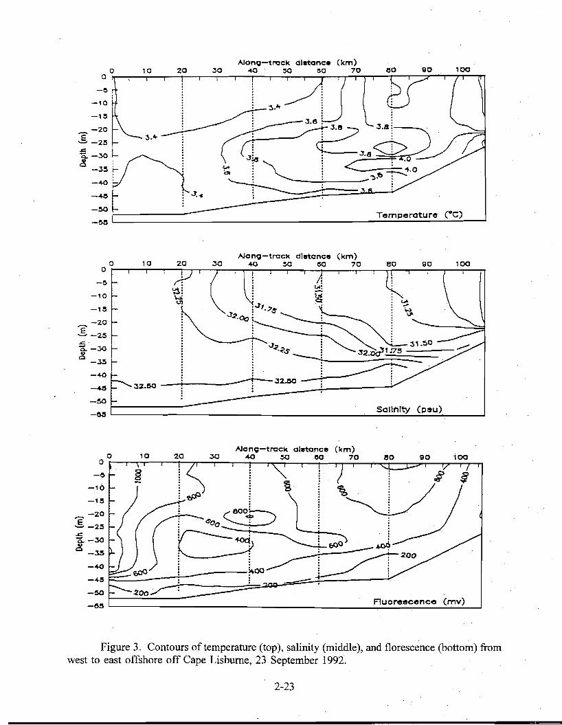
O·

-0

-10

-1~

........ -20

..§, -2~ ...:::: 'Q..-30 ~

-35

-040

-~

-~ Temperature C'C)

A1ono-trock dlstonce 0 10 20 ~O 040 ~ 00 90 100

.3:11

-o~

A1ono-trock dlstonce (km) 0 10 30 40 ~ 00 70 eo 90 100

0

-0

-10

-1~

........ -20

..§, -2~ ...:::: '

'Q..-30 ~

-3.5

-40

-~

-~ Salinity (psu)

-~

A1ono-trock dletonce (km)° 10 20 30 040 ~ 00 70 80 90 100 DrT""""'S:O---'-!7---r-r-r-""T"\-r---'--T~JT':""-r-::::t:::::t==~---y,.........7'l

-0 :;.: § ~

~10 ~. I 8l-l!~' I /=:: __~ <:0+ J . j ~ t: N ~ 1=",0 j~=: 1 ~ ~~~j200

~==~~__~:_-----;.t,.OO . .-~~ . i . :

-~ ~_.=..:.:::.:..._-----o~ L..- ......... ..:.,Fl..:.,u:.o:.r:..;e;;.:l!1;;.:c;..e:..."..:.,c.:.,.e.:..,..(:.;,m, _V':")_...J....

Figure 3. Contours of temperature (top), salinity (middle), and florescence (bottom) from west to east offshore off Cape Lisburne, 23 September 1991.

2-23

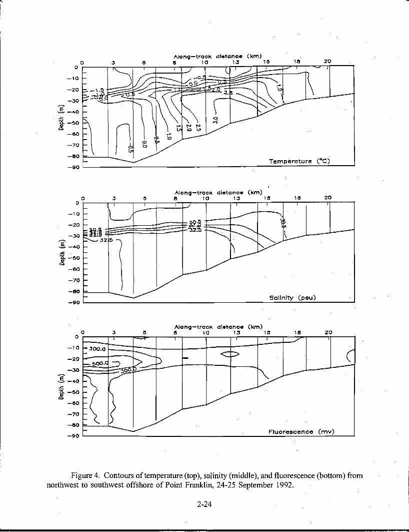
Temperature (OC)

-10

-20

-70

-eo F---""--~ -gO L "- ....:...___'___.......~

AJonCjl-trock dietonce (km) 0 e 10 1;' 1~ 16 20

0

-10

-20

-30 ........ 5-+0 .s= "13..-50 ~

-60

-70

-eo

-90 Sol1nlty (psu)

AJonCjl-trock dletonce (km) 0 oJ 15 e 10 1;' 1~ 18 20

0

-10

-20

-30 ......... 5-+0 .s=3- -50 Q

-60

-70

-eo Fluorescence (mv)

-90

Figure 4. Contours of temperature (top), salinity (middle), and fluorescence (bottom) from northwest to southwest offshore of Point Franklin, 24-25 September 1992.

2-24

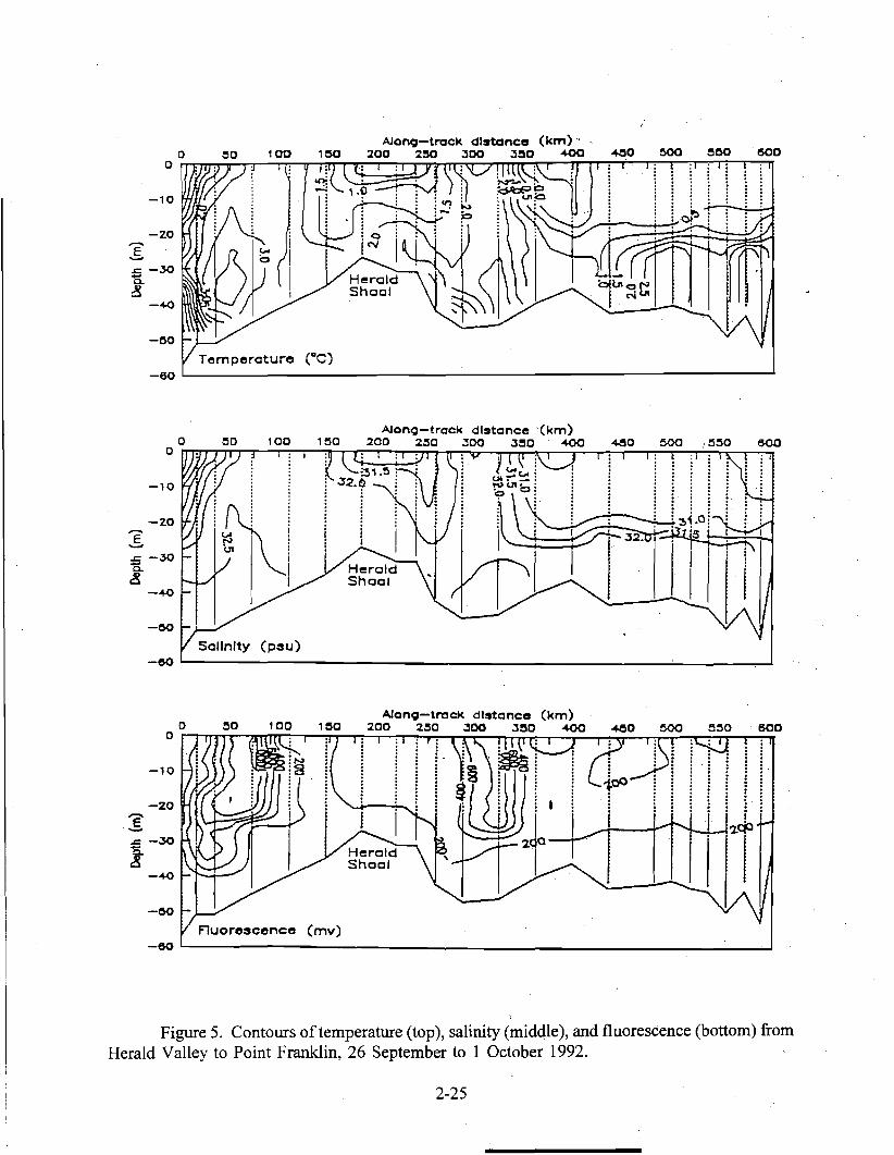
Alano-track dIstance (km)' , '00 200 2!50 .JOO .J~O _400

-10

-20

E-=[-30 ~

-00

Temperature ("C)

A1ano-trock dIstance -(km)

° °rn;TTirOrr°T""r--'°r°-:-r-''''':1°r°T"ir:-2"T0_O~....,2~O,.:°M~:5;;OO~~.J:;O;.:0=r_,...._-400:..:;.:::.......,~~.......,..,..:.:;.:....,.,..;~~ ...........:60:;0

_60L- ---l

~------------l.---.......,......l

-10

-20

E-

-00

-60 L---------

A1ano-track dIstance (km)

° °Fl"'"TT:nOn°:-:mtn'0TO;I'::151'10"r:2.:r0..:.O,.,.-7-20:r0:;....-rT:5:.:t00=-"TT1;;.J~;:0~r_-400=;.::...,r_:=;;:.:~..;:.:;::.._:T'"..;:;::;..._c_· ..:;:60:;0

-10

-20 ]: .= -30 !

-40

-00

-60 L-----­ .......,......l

Figure 5. Contours of temperature (top), salinity (middle), and fluorescence (bottom) from Herald Valley to Point Franklin, 26 September to 1 October 1992.

2-25

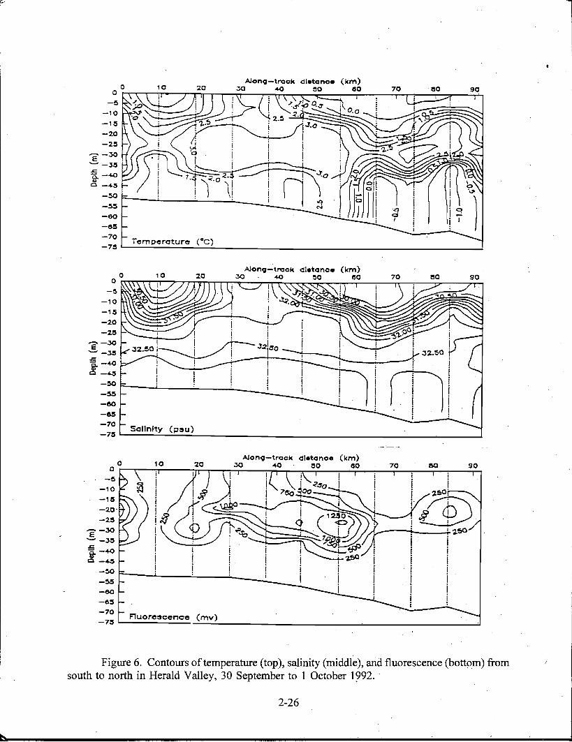
I

(km)

o 0t'\""",\;-",1rO_"j"""T'"rr-r-r""'"""'~_--r-~,.:..-.....-".......~_--:-......:.e;:.O_...,...........:.7;:.0-r-:-_·..:e;.0-..",_--=9,:...,0

---....---l

If!-,

-!>

-10

-1:1

-20 -2:1

e-30 - -3:1 ..c0.-+0 Q)o _~

-~ [--""-----.;..--.....:.-.__!­-~

-&0

-6:1

-70 -7:1

Temperature C"C)

AJon9-track dletanoe (km)

'--------.,;-~-----

_!>

-1 0

-1:1

-20 -2:1

e-30 --3!5 ..c0.-+0 ~-~

-~

-&0 -as -70

---------i i

mil . !. I - i . i

i :

o O~'\"'\'rr,1rO/-r,iT"2n°""l"'T"T"I'"7""'30r----:r-:"'I"'"40~~_.::""'~~i:0""",O::,"_.,..,:_=e;:..0--......:.n_____;"'"-...:,;......,-___?,.:., I !

~\ ~~'E:\:t::::.-

-50 [-_.l-_........:.__~__~

Sollnlty (psu)-715 I.----=--....;:.:.......;;..:...­ .......__---l

AJon9-t rack

o 0r-"'\_,1rO__lT2r°-,---,.~30,:...-"""':""r40,:..,......:........~-___;"'"--=:;:....~-..:.7;.0-.,.....--=50:;:........,....-..:9:,:...,0 _!> I!

-10 -115

-20­-2:1

e-30 --315 ..ci--+O o_~

-~ [-_.l-_........:.__......:....__~

-~ -&0

-6:1

-70 Fluorescence (mv)-715 L.... ­ ......;;_ .....:,;",;",;",;~---- ___:___:l

Figure 6. Contours of temperature (top), salinity (middle), and fluorescence (bottom) from south to north in Herald Valley, 30 September to 1 October 1?92..

2-26

:..':=

We next consider the three transects running perpendicular to the Chukotsk Peninsula at Cape Shmidt, Cape Vankarem, and Cape Uelen. Prominently featured on the Cape Shmidt section (Figure 7) is a wedge of cold, low-salinity water which extends offshore for approximately 120 km. Offshore of this point, and beneath the surface lies warmer, more saline BSW, and along the bottom is a mixture of RCW and BSW. With but one exception, the salinity contours adjacent to the coast slope upwards implying southeastward baroclinic flow. This coastally confined flow is the Siberian Coastal Current (SCC) discussed previously with respect to the Bering Strait transect. The SCC originates in the East Siberian Sea and is fed by ice-melt and coastal freshwater discharge (Coachman et al. 1975). Some Russian oceanographers suggest· that the source might extend as far west as the Lena River which drains into the Laptev Sea (V. Pavlov, Arctic and Antarctic Research Institute, St. Petersburg, Russia). Embedded within the SCC, approximately 50 km offshore, is an eddy or filament as suggested by the upward bowing of the isohalines. This featl,1re is associated with a near-bottom lens of warm, saline BSW water and could be one mechanism by which SCC waters mix with those from the Bering Sea (Coachman and Shigaev, 1992). Fluorescence values are extremely low within the SCC, but higher offshore in the BSW water mass.

As shown on the Cape Vankarem transect (Figure 8) SCC waters are both warmer and saltier which is probably a consequence· of mixing and entrainment of BSW into the SCe. However, the two water masses are clearly delineated by a front which intersects the "surface about 100 km offshore. Note again that there is a rapid increase in fluorescence on crossing the salinity front which separates the SCC from the Bering Shelf water.

There are several curious features observed along the Cape Uelen-Point Hope transect (Figure 9). First, the cold, low salinity flow of the SCC has collapsed to a narrow band confined to within 25 km of the coast. Apparently the bulk of the SCC has recirculated into the interior of the Chukchi Sea between Cape Uelen and Cape Van Karem. Although this data set cannot address this issue, the change in coastal orientation and bottom slope approximately midway between Cape Vankarem and Cape Uelen (see Figure 1) suggests that retroflection of the SCC might occur here. . f

Second the central portion of the transect is dominated by a large. anticyclonic (clockwise circulation) gyre centered approximately 100 km northeast of the Chukotsk Peninsula. This gyre has a radius of about 60 km and its center consists primarily of low salinity «32 psu) and relatively warm water (temperatures> 2.5 DC). The origin of the waters within the upper layers of the interior of this gyre cannot be determined precisely based upon the temperature and . salinity properties. Although these are similar to those characteristic of ACW, geographically, this water mass is typically confined . to the eastern Chukchi Sea (Coachman et al. 1975). However, mixtures of SCC water with BSW could also produce a water mass with the observed

. temperature and salinity properties. More detailed water mass analyses using the oxygen isotope and nutrient data collected on this cruise should resolve this issue.

Third, note that the stations nearest Point Hope have higher salinities than those within the gyre. Based upon earlier measurements (i:e., Coachman et al. 1975; Aagaard, 1988), we would have expected more dilute water at these stations as they typically lie within the northward flowing ACe. This observation in fact suggests that these low salinity waters were diverted offshore and contributed to the interior waters of the gyre.

2-27

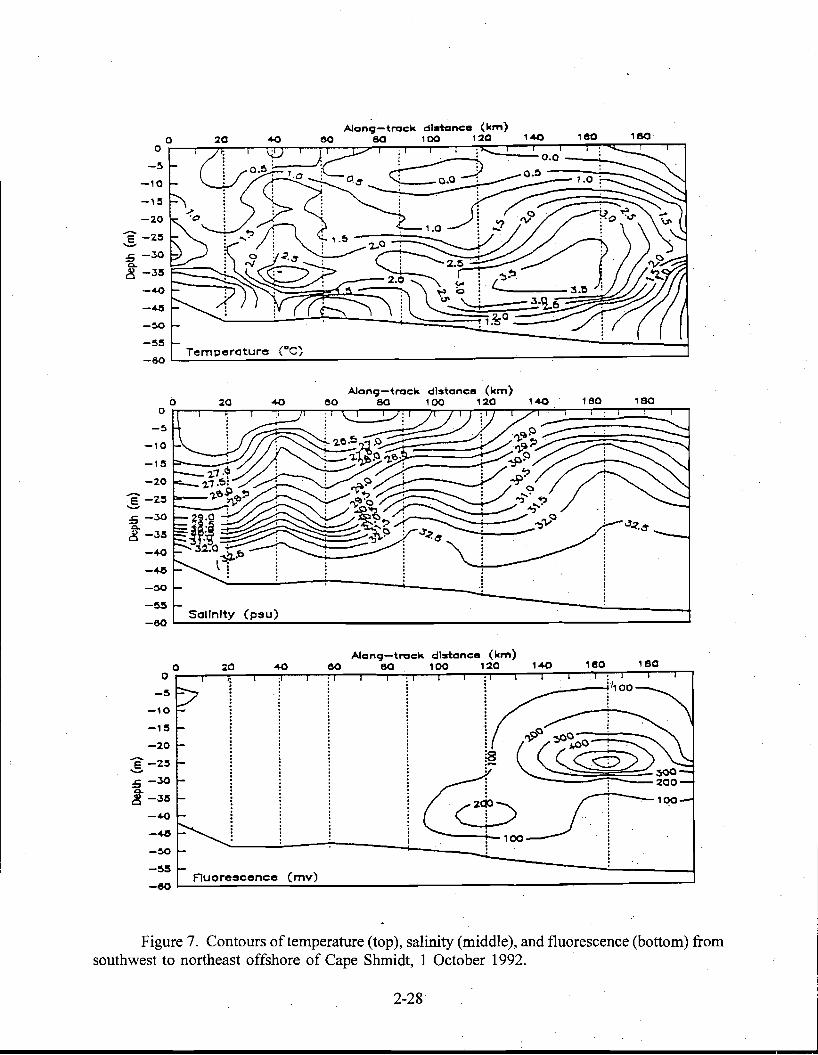
A1an9-track dl=nance (!em) o ~ ~ ~ ~ 100 1~ 1~ 1~ 1~

O;-----r---;,;:.--r---r.;;--.--n=--'"'T'""::n=--..,-..:..r:.......r-~:__r-"'T'""--r--r-~::::::::::_-.-.......,.__,

-5

-10

-1 :5

-20

E -2:5-

Figure 7. Contours of temperature (top), salinity (middle), and fluorescence (bottom) from southwest to northeast offshore of Cape Shmidt, 1 October 1992.

2-28

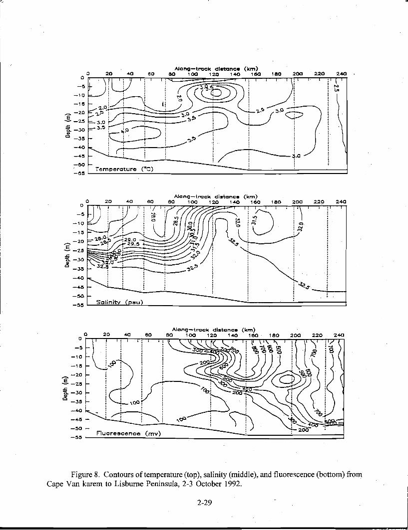
A1ono-t~c:k dhltanc:. (km) . 220o 20 eo 80 100 120 140 160 '80 200 240 o

-~: !; i !,. cSW i -1~ 2.o1~ : i ~ a ~:--......

E :/: ~. ~.~~: i : :; -2.'5 ~.O c....--r- . . -- : . : ~ =: I ~.~ F-1$), ~ ~ 1 ! I

~~~~"; . : -40 : i . ~ : . :

=: L_T.:.:e~m~i.~e~:o~~~u~r;e~i(;ac~)~===============~ =~==--=::=l-O:i ====='=1=·o=====:::j Alang-track di.tanc. (km)

1 22 40o °n'l-2TO-TTT~rOrr:eTOrr:::;80::r-:7:71~00'l~1::<l2~0~::::::>",140,..';;""'r-:...,60-;::--r-_'8,0---;1"';2...,OO,\-r-_,..O;....:r_2

_ 'l

~..,..

'-~--

--2.:5 ~~@:&. -30 ~

-5

-10

-1:5

-20 E

c! -~

-40

-~

-5().

L-.JS~c:!:lL!.!in~i!.!;t,-l.~!:!l-5:i

--!---1

-=:::::::===========::::j Along-track dl.tanc. (km)

o 20 40 eo 80 100 120 140 160· 180 200 220 240 °nT""...,....--r"':""""r-"'T"":'-r-,.""':Ir-.,...--rT-~~TT"'"T""..;.r~~rT=,nT~:......,~~""!T'"~:.:.....:-r-7"T,

-5

-10

-1 :5

-20 E - -2.:5

:&.-30 c! -3:5

-40

-~

-50

L_~F'~lu~o~r.::e:.:s~c:~e~n~c:::e~(~m~v!..) ~-----=::::============:::1-~:5

Figure 8. Contours of temperature (top), salinity (middle), and fluorescence (bottom) :from Cape Van karem to Lisburne Peninsula, 2-3 October 1992.

2-29

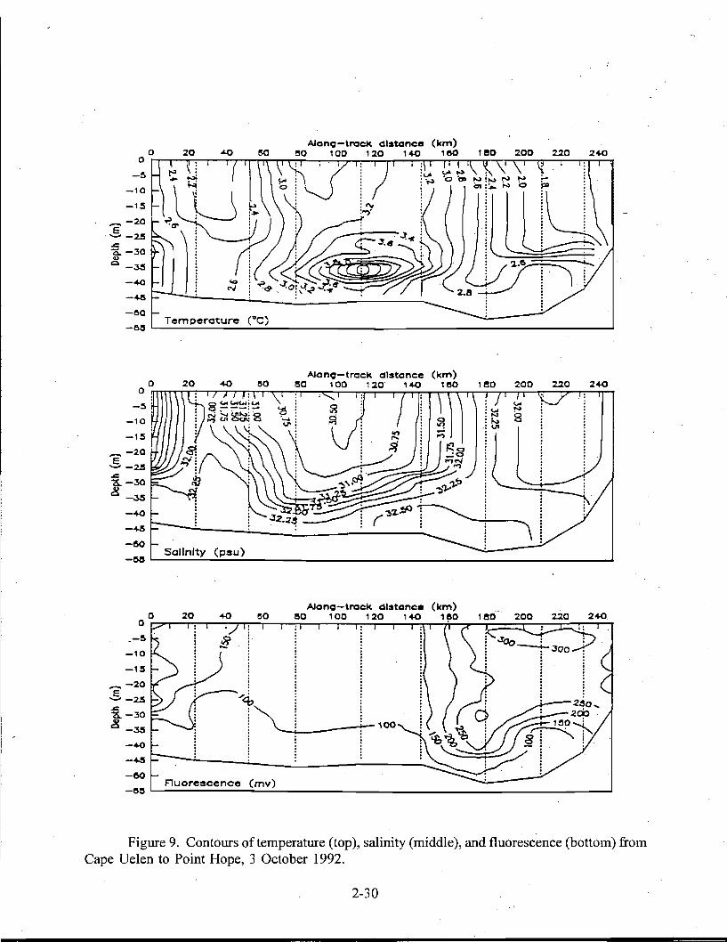
°P-~r"f"l~r'7lrT'l----'~i"""I----'i"""ITli"""I---':rr--;rr---J;==::x::---::::::r:::::::T:r-,

-60 -os I..----Fluorescence (mv)....;._....;.... ---l

Figure 9. Contours of temperature (top), salinity (middle), and fluorescence (bottom) from Cape Uelen to Point Hope, 3 October 1992.

2-30

AJono-track distance o W ~ ro ~ 100 1W 1~

-~

-10

-15

_-20

.-S-2S ..<:: Q. -30 G)

Q -3S

-40

--4-.5

-t!l0 Temperature ....;.......;.C"C)-os I..-__

°rr....-rr-:---r---r-71T""T"TT'""T'T"T"':"'1r--"'T"""'""'T-r-r-:-'"T""""'T"T-T'""";'Ir"T'""-rT-r-rr-Ir,,""""'t"'""'T"""-r.--r-.......IT--:r

~

AJono-track dIstance 20 40 ro eo 100 120· 1~

-~

-10

-15

_-20

-S-2S ..<:: 0.-30 c! -3S

-40

--4-.5

-60

-08 SalinIty (psu)

AJono-track dIstance o 20 40 !l0 eo 100 120 1~

_-5

-10

-1.5

_-20

-S-2S ..<:: 0. -30

.! -3S

-40

--4-.5

'r,,! .

~'00i "-----~i~---:-. .

(km) 1~ leo 200 220 2~

---l

(km) 180 leo :zoo 220 2~

(km) 1~O leo :zoo 220 2~.

The packing of the isohalines along the boundaries of this gyre imply locally swift ' baroclinic velocities, whereas the relatively homogeneous water within the center of the gyre is moving more slowly. Oxygen saturation values at the bottom and within the center of this gyre are less than 70% (Y. Sasaki and H. Ichii, personal communication) and provide additional indication of persistently weak flow within the center of the gyre. Strong horizontal current shear (implied by the strong salinity gradient and opposing slopes of the isohalines) is encountered on crossing the southeastward flow of the SCC and the northwestward flow on the southern portion of the gyre. This, divergent shear will cause water to upwell between these flows and this effect is suggested by the uplift of the 32.2 psu from 40 meters depth beneath the gyre center to about 20 m depth within the divergence zone. .

Fluorescence values are substantially lower than the maxima observed in previous transects. In large part, these low fluorescence values are associated with the prevalence of ACW and SCC waters observed on this transect. Lowest fluorescence values are again observed within the SCc.

The last cross-section shown is the reoccupation of the Bering Strait transect (Figure 10). Although temperatures are about 2°C lower than those observed on the first occupation, little of this cooling can be a result of heat loss to the atmosphere as winds were calm and air temperatures were nearly equal to sea surface temperatures, throughout most of the cruise. Rather, these differences must reflect a circulation change which resulted in the advection of cooler and saltier waters through the strait. In contrast to the first occupation, the, data from this section shows northward baroclinic flow within the ACC on the east side of the strait. In the western channel southward baroclinic flow is observed within a wedge extending 25 kIn offshore at the surface to about 5 kIn offshore at the bottom. Water within this southward flow consists of a mixture of SCC water with BSW and ACW.

SUMMARY

Hydrographic results from fall 1992 have delineated the northward spreading of Pacific waters throughout the Chukchi Sea. The Bering' Shelf fraction of these' waters generally has higher fluorescence levels than the other shelf water components, consistent with it being enriched in particulate organic carbon. Persistent northward flow of this carbon-rich water to the, east of Herald Shoal and along the east flank of Herald Canyon suggest that this northward flow could be a source of carbon to the benthic communities on the outer shelf of the northeast Chukchi Sea. As discussed in Chapter 3 resolving the circulation on the outer shelf is an important issue to be addressed in this regard. Enhanced primary production rates are also implied by the elevated fluorescence levels (and oxygen supersaturation) along the ice-edge overlying Barrow Canyon. If true, this productivity could also be an important carbon source to the benthic and fish communities of this region. '

Observations from Bering Strait indicate that, at least occasionally, a portion of the Siberian Coastal Current flows southward along the west coast of Bering Strait. However, there is a significant reduction in the mass transport in this current between Cape Van karem and Bering Strait. Much of this flow must retroflect between' these two regions, and mix and be recirculated throughout the Chukchi Sea. Little is known -about this current but because of concerns regarding massive pollutant discharges into the rivers feeding the shelf seas of Eurasia (including the East Siberian Sea) we advise more emphasis be placed on this cuqent and its influence on the Chukchi Sea in the future. '

2-31

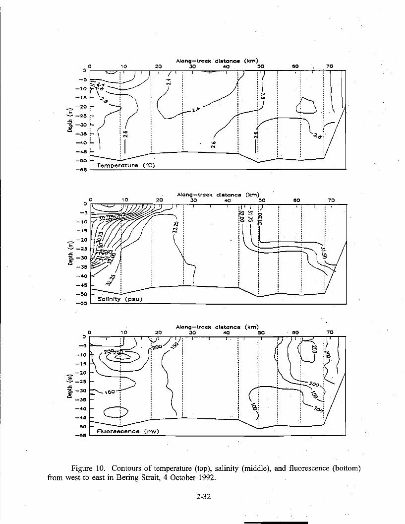
j. NI~ .. ::.

-50

O;-~O:::-7"":'....---r-.---r:---r-7"'"'T---:----':--""""'=_-'----:-"'--":"T'";--"""T---,-:--r---:-....--s'T

-0

-10

-15

-20

-2.5

i:S.-.JO

-~

AlonQ-track ·dl.tance (km) o 10 20 .JO ~ ~ eo 70

:; U.E -

1~i~

~ i l~ r.!

I '~l ,:.

. Temperature (DC)-00 I....-.:...:.:~..:.;,..~::..:.....:---...:.....:...;:.....-_--------------------_~

Figure 10. Contours of temperature (top), salinity (middle), and fluorescence (bottom) from west to east in Bering Strait, 4 October 1992.

2-32

CHAPTER 3

CIRCULATION AND FORMATION OF COLD, SALINE WATER ON THE NORTHEAST CHUKCHI SHELF

THOMAS J. WEINGARTNER

Institute of Marine Science, University of Alaska Fairbanks Fairbanks, Alaska 99775-7220

Abstract.-Five current meter moorings were deployed in the northeast Chukchi Sea from October 1991 through August and/or September 1992. Four were deployed in the Alaska Coastal Current; two offshore of Cape Lisburne and two in Barrow Canyon. A fifth mooring was deployed in the central Chukchi Sea, east of Herald Shoal and approximately 250 km to the west of Barrow Canyon.

Current variations were: 1) spatially coherent throughout the northeast Chukchi Sea and 2) significantly coherent with the local wind field. Current variations offshore of Cape Lisburne were more coherent with winds over the northern Bering Sea than the winds over the northern Chukchi Sea suggesting that here the coastal current's dynamics are, in part, tied to sea-level adjustments associated with wind-driven transport variations in the Bering Strait.

At the Herald Shoal mooring site, the mean monthly flow was northward to contrast to earlier inferences based upon limited hydrography. Temperature and salinity properties are consistent with those for the nutrient- and carbon-rich Bering Sea Water mass flowing northward through the western channel of Bering Strait. Fall CTD casts and fluorescence values are also consistent with this interpretation and suggest that this flow might be a substantial source of carbon for the benthic communities on the outer Chukchi shelf.

On a monthly mean basis the shelf circulation was remarkably steady and swift throughout most of the year. However, from November 1991 through January 1992, when strong northeasterly winds blew over the Chukchi and northern Bering seas, near stagnant flow conditions ensued and the alongshore coherence of the coastal current was disrupted. By early December, shelf water temperatures had cooled to the freezing point and a large polynya system developed along Alaska's northwest coast. Ice production and the associated salt flux within these polynyas contributed to the formation of a shelf water mass with temperatures near the freezing point and salinities > 34 psu. Formation of this water mass was enhanced by the weak circulation which effectively increased the residence time of water parcels within the polynyas thereby allowing salinities to increase to an extent greater than would be expected if swift flow had persisted. Production of this dense water is therefore seen as a rectified response of the ice cover and the ocean to strong northeasterly winds which: 1) created the polynyas, 2) enhanced oceanic heat loss and ice production, and 3) led to weak shelf circulation.

With abatement of the strong northeasterly winds in late January, the normal shelf circulation mode was reestablished and most of the cold, saline water was flushed through Barrow Canyon over the course of the next two months. However, a substantial fraction of this dense water also drained to the northwest and through the broad channel between Hearld and Hanna Shoals.

3-1

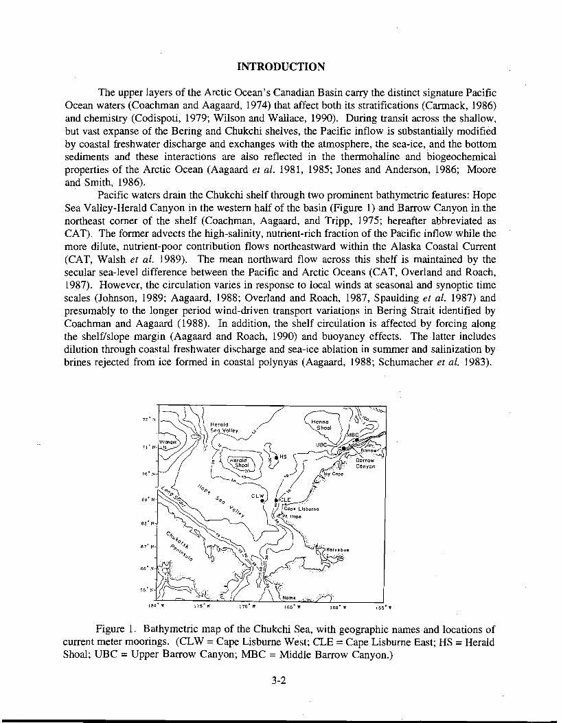
INTRODUCTION

The upper layers of the Arctic Ocean's Canadian Basin carry the distinct signature Pacific Ocean waters (Coachman and Aagaard, 1974) that affect both its stratifications (Carmack, 1986) and chemistry (Codispoti, 1979; Wilson and Wallace, 1990). During transit across the shallow, but vast expanse of the Bering and Chukchi shelves, the Pacific inflow is SUbstantially modified by coastal freshwater discharge and exchanges with the atmosphere, the sea-ice, and the bottom sediments and these interactions are also reflected in the thermohaline and· biogeochemical properties of the Arctic Ocean (Aagaard et al. 1981, 1985; Jones and Anderson, 1986; Moore and Smith, 1986).

Pacific waters drain the Chukchi shelf through two prominent bathymetric features: Hope Sea Valley-Herald Canyon in the western half of the basin (Figure 1) and Barrow Canyon in the northeast corner of the shelf (Coachman, Aagaard, and Tripp, 1975; hereafter abbreviated as CAT). The former advects the high-salinity, nutrient-rich fraction of the Pacific inflow while the more dilute, nutrient-poor contribution flows northeastward within the Alaska Coastal Current (CAT, Walsh et al. 1989). The mean northward flow across this shelf is maintained by the secular sea-level difference between the Pacific and Arctic Oceans (CAT, Overland and Roach, 1987). However, the circulation varies in response to local winds at seasonal and synoptic time scales (Johnson, 1989; Aagaard, 1988; Overland and Roach, 1987, Spaulding et al. 1987) and presumably to the longer period wind-driven transport variations in Bering Strait identified by Coachman and Aagaard (1988). In addition, the shelf circulation is affected by forcing along the shelf/slope margin (Aagaard and Roach, 1990) and buoyancy effects. The latter includes dilution through coastal freshwater discharge and sea-ice ablation in summer and salinization by brines rejected from ice formed in coastal polynyas (Aagaard, 1988; Schumacher et al. 1983).

Figure 1. Bathymetric map of the Chukchi Sea, with geographic names and locations of current meter moorings. (CLW =Cape Lisburne West; CLE =Cape Lisburne East; HS =Herald Shoal; UBC =Upper Barrow Canyon; MBC =Middle Barrow Canyon.)

3-2

The cold, saline water formed by brine addition is particularly important to the long-term integrity of the Arctic Ocean's halocline (Aagaard et aI., 1981, Killworth and Smith, 1984; Bjork, 1989). In the western Arctic, the principal sources of brines are the coastal polynyas formed in winter on the northern Bering shelf and in the northeast Chukchi Sea (Cavalieri and Martin, in revision; hereafter abbreviated as CM). Dense water formed within the latter presumably drains through Barrow Canyon. Apparently, however, there are years when the cold, saline water formed within these polynyas is either not dense enough to ventilate the halocline or it follows a different path to the Arctic Ocean (Aagaard and Roach, 1990).. CM show considerable interannual differences in both the size and the duration of polynya events on the northeast shelf and these are important factors affecting the volume and properties of the dense water formed. While the shelf circulation is important transporting dense water, it might also play a role in establishing conditions favorable to the formation of cold, saline water.

This study was largely motivated by needs to understand better the circulation and water mass properties on the northeastern shelf (between Herald Shoal and Barrow Canyon) where gas and oil exploration activities were underway. Particular emphasis was to be placed on the north central shelf (between Hanna and Herald Shoals) where the circulation is poorly known. In addition, this program provided an opportunity to add to the existing set of current measurements from Barrow Canyon in order to describe: 1) interannual variations in the circulation and water mass properties of the northeastern shelf, 2) the relationship between current variations in the coastal flow and the north central shelf, and 3) the vertical and along-canyon structure of near-bottom flows of cold, saline outflows as well as intrusions of Arctic Intermediate Water (AIW, [cf. Aagaard et al. 1985]) upwelled along the continental slope and within the Atlantic layer of the Arctic Ocean. With these goals in mind, the initial plan called for three moorings to be deployed on the north central shelf and two moorings in Barrow Canyon. However, extensive ice prevented the ship from reaching three of the planned positions. As a result, the moorings were deployed as follows: UBC (Upper Barrow Canyon) at the same location as the mooring described by Aagaard et al. (1985), MBC (Middle Barrow Canyon) near the center of the canyon approximately midway along its longitudinal axis, HS (Herald Shoal) in the depression to the east of Herald Shoal, CLW and CLE (Cape Lisburne West and East, respectively) offshore of Cape Lisburne. These last two mooring sites were in the same vicinity as those deployed by Aagaard (1988) and Coachman and Aagaard (1981). As it turned out, these proved useful in understanding the mid-winter production and transport of brine across the northeast shelf. Figure 1 shows the mooring locations.

The mooring data are augmented with satellite imagery obtained from the Special Sensor Microwave/lmager (SSM/I) and the Advanced Very High Resolution Radiometer (AVHRR). In conjunction with regional meteorological data, the imagery guides the interpretation of temperature and salinity measurements obtained by the current meters.

METHODS

Each mooring consisted of a variable number of Aanderaa model RCM? and RCM4 current meters equipped with thermistors and conductivity cells. The topmost current meter at moorings UBC and MBC included a pressure sensor to monitor vertical mooring motion. Tables 1a and 1b provide specifics on the moorings and instrument record· lengths. Each mooring included one current meter suspended three meters above the bottom and one current meter, less its vane, set in a well on the anchor. In Barrow Canyon, mooring UBC incorporated an additional instrument 12 meters above the bottom andMBC included instruments at 12, 18, and

3-3

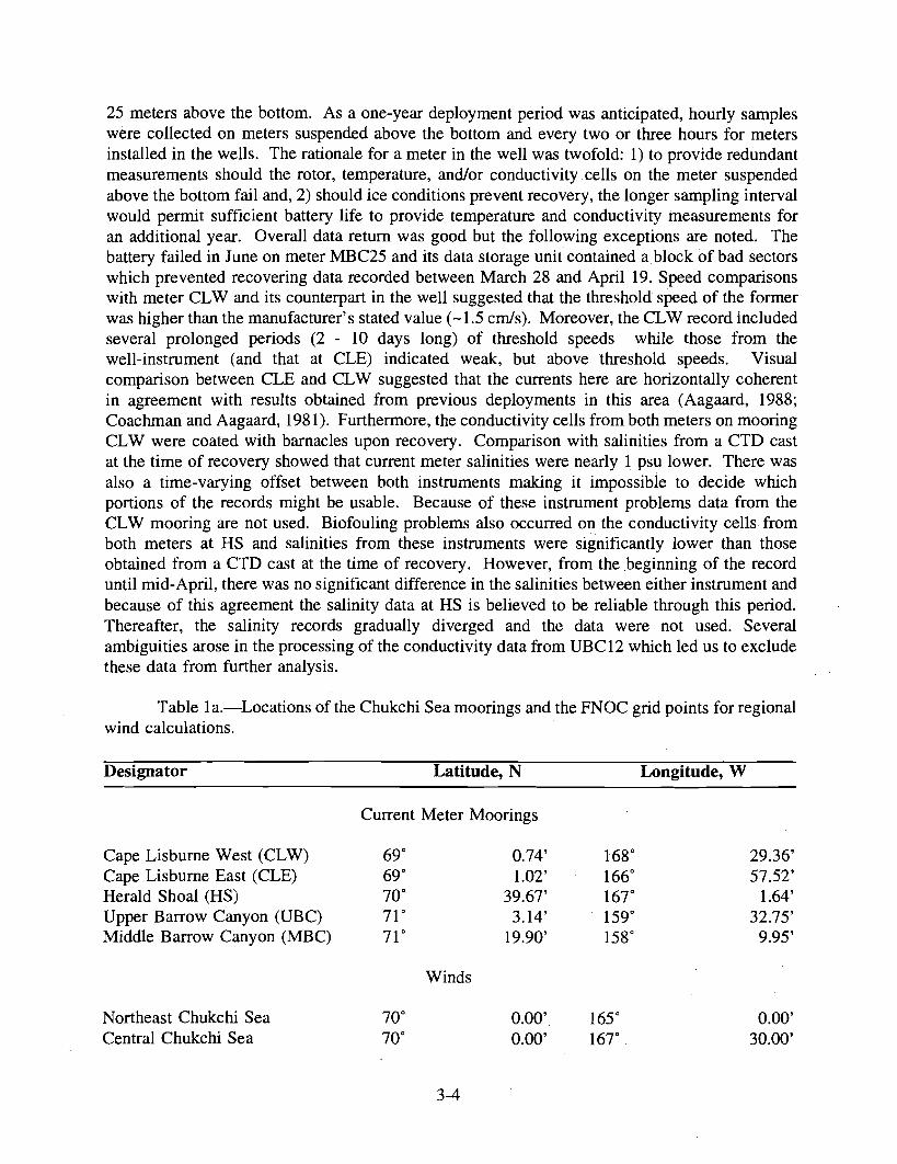
25 meters above the bottom. As a one-year deployment period was anticipated, hourly samples were collected on meters suspended above the bottom and every two or three hours for meters installed in the wells. The rationale for a meter in the well was twofold: 1) to provide redundant measurements should the rotor, temperature, andlor conductivity cells on the meter suspended above the bottom fail and, 2) should ice conditions prevent recovery, the longer sampling interval would permit sufficient battery life to provide temperature and conductivity measurements for an additional year. Overall data return was good but the following exceptions are noted. The battery failed in June on meter MBC25 and its data storage unit contained ablock of bad sectors which prevented recovering data recorded between March 28 and April 19. Speed comparisons with meter CLW and its counterpart in the well suggested that the threshold speed of the former was higher than the manufacturer's stated value (-1.5 cm/s). Moreover, the CLW record included several prolonged periods (2 - 10 days long) of threshold speeds while those from the well-instrument (and that at CLE) indicated weak, but above threshold speeds. Visual comparison between CLE and CLW suggested that the currents here are horizontally coherent in agreement with results obtained from previous deployments in this area (Aagaard, 1988; Coachman and Aagaard, 1981). Furthermore, the conductivity cells from both meters on mooring CLW were coated with barnacles upon recovery. Comparison with salinities from a CTD cast at the time of recovery showed that current meter salinities were nearly 1 psu lower. There was also a time-varying offset between both instruments making it impossible to decide which portions of the records might be usable. Because of these instrument problems data from the CLW mooring are not used. Biofouling problems also occurred on the conductivity cells from both meters at HS and salinities from these instruments were significantly lower than those obtained from a CTD cast at the time of recovery. However, from the beginning of the record until mid-April, there was no significant difference in the salinities between either instrument and because of this agreement the salinity data at HS is believed to be reliable through this period. Thereafter, the salinity records gradually diverged and the data were not used. Several ambiguities arose in the processing of the conductivity data from UBC12 which led us to exclude these data from further analysis.

Table 1a.-Locations of the Chukchi Sea moorings and the FNOC grid points for regional wind calculations.

Designator Latitude, N Longitude, W

Cape Lisburne West (CLW) Cape Lisburne East (CLE) Herald Shoal (HS) Upper Barrow Canyon (UBC) Middle Barrow Canyon (MBC)

Northeast Chukchi Sea Central Chukchi Sea

Current Meter Moorings

690 0.74'

69 0 1.02' 70 0 39.67' 71

0 3.14' 71

0 19.90'

Winds

70 0

0.00'. 70 0 0.00'

168 0

1660

167" 1590

1580

165 0

167" .

29.36' 57.52'

1.64' 32.75'

9.95'

0.00' 30.00'

3-4

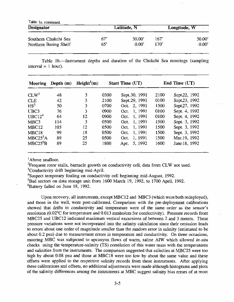
Table lao continued.

Designator Latitude, N Longitude, W

Southern Chukchi Sea 30.00' 167" 30.00' Northern Bering Shelf 0.00' 1700 0.00'

Table lb.-Instrument depths and duration of the Chukchi Sea moorings (sampling interval = 1 hour).

Mooring Depth (m) Height1(m) Start Time (UT) End Time (UT)

CLW2 48 3 0300 Sept.30, 1991 2100 Sept22, 1992 CLE HS3

42 50

3 3

2100 0700

Sept.29, 1991 Oct. 2, 1991

0100 1500

Sept23, 1992 Sept27, 1992

UBC3 UBC124

76 64

3 12

0900 0900

Oct. Oct.

1, 1991 1, 1991

0100 0100

Sept. 4, 1992 Sept. 4, 1992

MBC3 114 3 0500 Oct. 1, 1991 1500 Sept. 3, 1992 MBC12 105 12 0500 Oct. 1, 1991 1500 Sept. 3, 1992 MBC18 MBC255A MBC256B

99 89 89

18 25 25

0500 0500 1800

Oct. Oct. Apr.

1, 1991 1, 1991 5, 1992

1500 1500 1600

Sept. 3, 1992 Mar.19, 1992 June 18, 1992

I Above seafloor. 2Frequent rotor stalls, barnacle growth on conductivity cell, data from CLW not used. 3Conductivity drift beginning mid-April. 4Suspect temporary fouling on conductivity cell beginning mid-August, 1992. 5Bad sectors on data storage unit from 1600 March 19, 1992, to 1700 April, 1992. 6Battery failed on June 18, 1992.

Upon recovery, all instruments, except MBC12 and MBC3 (which were both redeployed), and those in the well, were post-calibrated. Comparison with the pre-deployment calibrations showed that drifts in conductivity and temperature were of the same order as the sensor's resolution (0.02°C for temperature and 0.013 mmho/cm for conductivity). Pressure records from MBC25 and UBC12 indicated maximum vertical excursions of between 2 and 3 meters. These pressure variations were not incorporated into the salinity calculation since their omission leads to errors about one order of magnitude smaller than the random error in salinity (estimated to be about 0.2 psu) due to measurement errors in temperature and conductivity. On three occasions, mooring MBC was subjected to upcanyon flows of warm, saline AIW which allowed in-situ checks using the temperature-salinity (TS) correlation of this water mass with the temperatures and salinities from the instruments. The comparison suggested that salinities at MBC25 were too high by about 0.08 psu and those at MBC18 were too low by about the same value and these offsets were applied to the respective salinity records from these instruments. After applying these calibrations and offsets, no additional adjustments were made although histograms and plots of the salinity differences among the instruments at MBC suggest salinity bias errors of at most

3-5

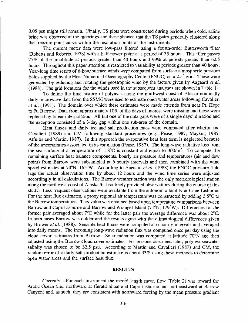
0.05 psu might still remain. Finally, TS plots were constructed during periods when cold, saline brine was observed at the moorings and these showed that the TS pairs generally clustered along the freezing point curve within the resolution limits of the instruments.

The current meter data were low-pass filtered using a fourth-order Butterworth filter (Roberts and Roberts, 1978) with a half-power point at a period of 35 hours. This filter passes 77% of the amplitude at periods greater than 40 hours and 99% at periods greater than 62.5 hours. Throughout this paper attention is restricted to variability at periods greater than 40 hours. Year-long time series of 6-hour surface winds were computed from surface atmospheric pressure fields supplied by the Fleet Numerical Oceanography Center (FNOC) on a 2.5° grid. These were generated by reducing and rotating the geostrophic wind by the factors given by Aagaard et al. (1988). The grid locations for the winds used in the subsequent analyses are shown in Table 1a.

To define the time history of polynyas along the northwest coast of Alaska nominally daily microwave data from the SSMII were used to estimate open water areas following Cavalieri et al. (1991). The domain over which these estimates were made extends from near Pt. Hope to Pt. Barrow. Data from approximately 10% of the days of interest were missing and these were replaced by linear interpolation. All but one of the data gaps were of a single days' duration and the exception consisted of a 3-day gap within one sub-area of the domain.

Heat fluxes and daily ice and salt production rates were computed after Martin and Cavalieri (1989) and CM following standard procedures (e.g., Pease, 1987; Maykut, 1985; Alfultis and Martin, 1987). In this approach the evaporative heat loss term is neglected because of the uncertainties associated in its estimation (Pease, 1987). The long-wave radiative loss from the sea surface at a temperature of -1.8°C is constant and equal to 300/m2

. To compute the remaining surface heat balance components, hourly air pressure and temperatures (air and dew point) from Barrow were subsampled at 6-hourly intervals and then combined with the wind speed estimates at 700 N, 165°W. According to Aagaard et al. (1988) the FNOC pressure field lags the actual observation time by about 12 hours and the wind time series were adjusted accordingly in all calculations. The Barrow weather station was the only meteorological station along the northwest coast of Alaska that routinely provided observations during the course of this study. Less frequent observations were available from the autonomic facility at Cape Lisburne. For the heat flux estimates, a proxy regional air temperature was constructed by adding 3.5°C to the Barrow temperatures. This value was obtained based upon temperature comparisons between Barrow and Cape Lisburne and Barrow and Wrangel Island (71 oN, 179°W). Differences for the former pair averaged about 7°C while for the latter pair the average difference was about 2°C. In both cases Barrow was colder and the results agree with the climatological differences given by Brower et ai. (1988). Sensible heat fluxes were computed at 6-hourly intervals and averaged into daily means. The incoming long-wave radiation flux was computed once per day using the cloud cover estimates from Barrow. Solar radiation was computed at latitude 700 N and then adjusted using the Barrow cloud cover estimates. For reasons described later, polynya seawater salinity was chosen to be 32.5 psu. According to Martin-and Cavalieri (1989) and CM, the random error of a daily salt production estimate is about 33% using these methods to determine open water areas and the surface heat flux.

RESULTS

Currents.-For each instrument the record length mean flow (Table 2) was toward the Arctic Ocean (i.e., northward at Herald Shoal and Cape Lisburne and northeastward at Barrow Canyon) and, as such, they are consistent with northward forcing by the mean pressure gradient

3-6

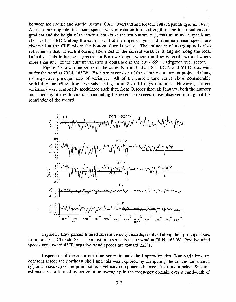
between the Pacific and Arctic Oceans (CAT, Overland and Roach, 1987; Spaulding etal. 1987). At each mooring site, the mean speeds vary in relation to the strength of the local bathymetric gradient and the height of the instrument above the sea bottom, e.g., maximum mean speeds are observed at UBC 12 along the eastern wall of the upper canyon and minimum mean speeds are observed at the CLE where the bottom slope is weak. The influence of topography is also reflected in that, at each mooring site, most of the current variance is aligned along the local isobaths. This influence is greatest in Barrow Canyon where the flow is rectilinear and where more than 95% of the current variance is contained in the 50° - 65° DT (degrees true) sector.

Figure 2 shows time series of the currents from CLE, HS, UBC12 and MBC12 as well as for the wind at 700 N, 165°W. Each series consists of the velocity component projected along its respective principal axis of variance. All of the current time series show considerable variability including flow reversals lasting from 2 to 10 days duration. However, current variations were seasonally modulated such that, from October through January, both the number and intensity of the fluctuations (including the reversals) exceed those observed throughout the remainder of the record.

75 USC 3

~ _:~ -t----\t-tt-++jH-1t-tft-jhl~[\~~/JJl'vir $ -50 ~ r-r­

-75 -100

HS

~.tJcnE_ =~o~ l~Ll,~fi-,~_~-L",1~-===tF-~'I-1IHIt1~ec-,. n AI A:""":"i --vvvWV-"V'-V\J'v ~- v:v:_ IJ.,,i:~n<~V :<Y tr

I :II 30 JO 28 211 2t 28 U n n 20 Ie

OCT NOV DEC JAN FEB MAR APR MAY JUN JUL AUG SEP 1991 1992

Figure 2. Low-passed filtered current velocity records, resolved along their principal axes, from northeast Chukchi Sea. Topmost time series is of the wind at 70DN, 165DW. Positive wind speeds are toward 43°T, negative wind speeds are toward 223°T.

Inspection of these current time series imparts the impression that flow variations are coherent across the northeast shelf and this was explored by computing the coherence squared (y) and phase (<I» of the principal axis velocity components between instrument pairs. Spectral estimates were formed by convolution averaging in the frequency domain over a bandwidth of

3-7

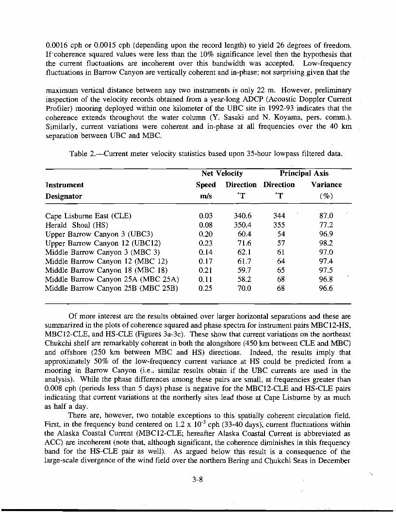
0.0016 cph or 0.0015 cph (depending upon the record length) to yield 26 degrees of freedom. If coherence squared values were less than the 10% significance level then the hypothesis that the current fluctuations are incoherent over this bandwidth was accepted. Low-frequency fluctuations in Barrow Canyon are vertically coherent and in-phase; not surprising given that the

maximum vertical distance between any two instruments is only 22 m. However, preliminary inspection of the velocity records obtained from a year-long ADCP (Acoustic Doppler Current Profiler) mooring deployed within one kilometer of the UBC site in 1992-93 indicates that the coherence extends throughout the water column (Y. Sasaki and N. Koyama, pers. comm.). Similarly, current variations were coherent and in-phase at all frequencies over the 40 km separation between UBC and MBC.

Table 2.-Current meter velocity statistics based upon 35-hour lowpass filtered data.

Net Velocity Principal Axis

Instrument Speed Direction Direction Variance aT aTDesignator mls (%)

Cape Lisburne East (CLE) 0.03 340.6 344 87.0 Herald Shoal (HS) 0.08 350.4 355 77.2 Upper Barrow Canyon 3 (UBC3) 0.20 60.4 54 96.9 Upper Barrow Canyon 12 (UBC12) 0.23 71.6 57 98.2 Middle Barrow Canyon 3 (MBC 3) 0.14 62.1 61 97.0 Middle Barrow Canyon 12 (MBC 12) 0.17 61.7 ·64 97.4 Middle Barrow Canyon 18 (MBC 18) 0.21 59.7 65 97.5 Middle Barrow Canyon 25A (MBC 25A) 0.11 58.2 68 96.8 Middle Barrow Canyon 25B (MBC 25B) 0.25 70.0 68 96.6

Of more interest are the results obtained over larger horizontal separations and these are summarized in the plots of coherence squared and phase spectra for instrument pairs MBC12-HS, MBC12-CLE, and HS-CLE (Figures 3a-3c). These show that current variations on the northeast Chukchi shelf are remarkably coherent in both the alongshore (450 km between CLE and MBC) and offshore (250 km between MBC and HS) directions. Indeed, the results imply that approximately 50% of the low-frequency current variance at HS could be predicted from a mooring in Barrow Canyon (i.e., similar results obtain if the UBC currents are used in the analysis). While the phase differences among these pairs are small, at frequencies greater than 0.008 cph (periods less than 5 days) phase is negative for the MBC12-CLE and HS-CLE pairs indicating that current variations at the northerly sites lead those at Cape Lisburne by as much as half a day.

There are, however, two notable exceptions to this spatially coherent circulation field. First, in the frequency band centered on 1.2 x 10-3 cph (33-40 days), current fluctuations within the Alaska Coastal Current (MBC12-CLE; hereafter Alaska Coastal Current is abbreviated as ACC) are incoherent (note that, although significant, the coherence diminishes in this frequency band for the HS-CLE pair as well). As argued below this result is a consequence of the large-scale divergence of the wind field over the northern Bering and Chukchi Seas in December

3-8

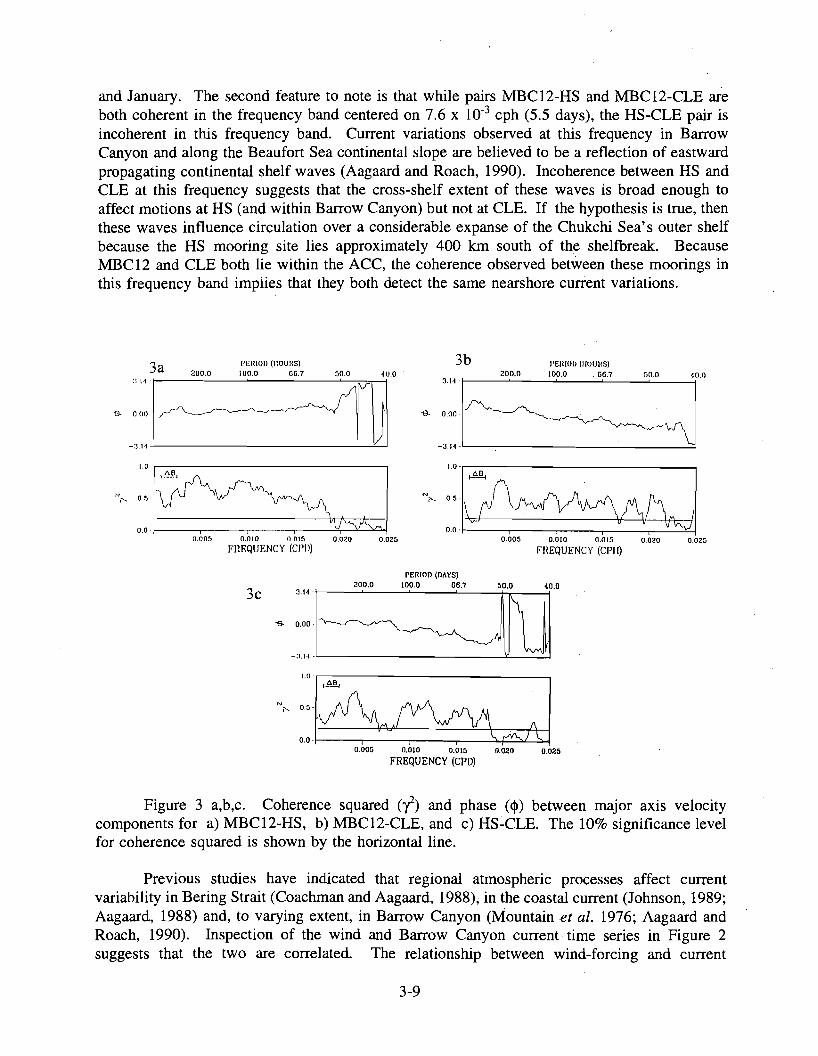
and January. The second feature to note is that while pairs NffiCI2-HS and MBCI2-CLE are both coherent in the frequency band centered on 7.6 x 10-3 cph (5.5 days), the HS-CLE pair is incoherent in this frequency band. Current variations observed at this frequency in Barrow Canyon and along the Beaufort Sea continental slope are believed to be a reflection of eastward propagating continental shelf waves (Aagaard and Roach, 1990). Incoherence between HS and CLE at this frequency suggests that the cross-shelf extent of these waves is broad enough to affect motions at HS (and within Barrow Canyon) but not at CLE. If the hypothesis is true, then these waves influence circulation over a considerable expanse of the Chukchi Sea's outer shelf because the HS mooring site lies approximately 400 km south of the shelfbreak. Because MBC 12 and CLE both lie within the ACC, the coherence observed between these moorings in this frequency band implies that they both detect the same nearshore current variations.

3a I'EHlOIl (1I0UIIS) 3b I'EHlOI) (1I0UIIS)

~ _::::1,-__2_00_'0__10_0'_0__66_.7__5_?_0_-,,-u_l' ~ _: ~:I "" '00.' .~, '?' r N" ~:I~~ .~I . !\~M::I\~~· ;1~ .nnn ~U5~

"0

. "" ui/~1rQ0.0 i 0.0 - -----r-----,---,..---r-...:....-.:.l::... 0.005 0.010 (l.Ot5 0.020 0.025 0.005 0.010 0.0\5 0.020 0.025

FREQUENCY (CI'Il) FHEQUENCY (CPII)

PERIOD (DAYS)

J.t4_1~200'006.7 50.0 40.0100.03c

"S 0.00··

-:1.14-.

"0 ::I~GY:\LL~A] 0.005 0.010 0.015 0.020 0.025

FREQUENCY (CPO)

Figure 3 a,b,c. Coherence squared (i) and phase ($) between major axis velocity components for a) MBCI2-HS, b) MBCI2-CLE, and c) HS~CLE. The 10% significance level for coherence squared is shown by the horizontal line.

Previous studies have indicated that regional atmospheric processes affect current variability in Bering Strait (Coachman and Aagaard, 1988); in the coastal current (Johnson, 1989; Aagaard, 1988) and, to varying extent, in Barrow Canyon (Mountainet aI. 1976; Aagaard and Roach, 1990). Inspection of the wind and Barrow Canyon current time series in Figure 2 suggests that the two are correlated. The relationship between wind-forcing and current

3-9

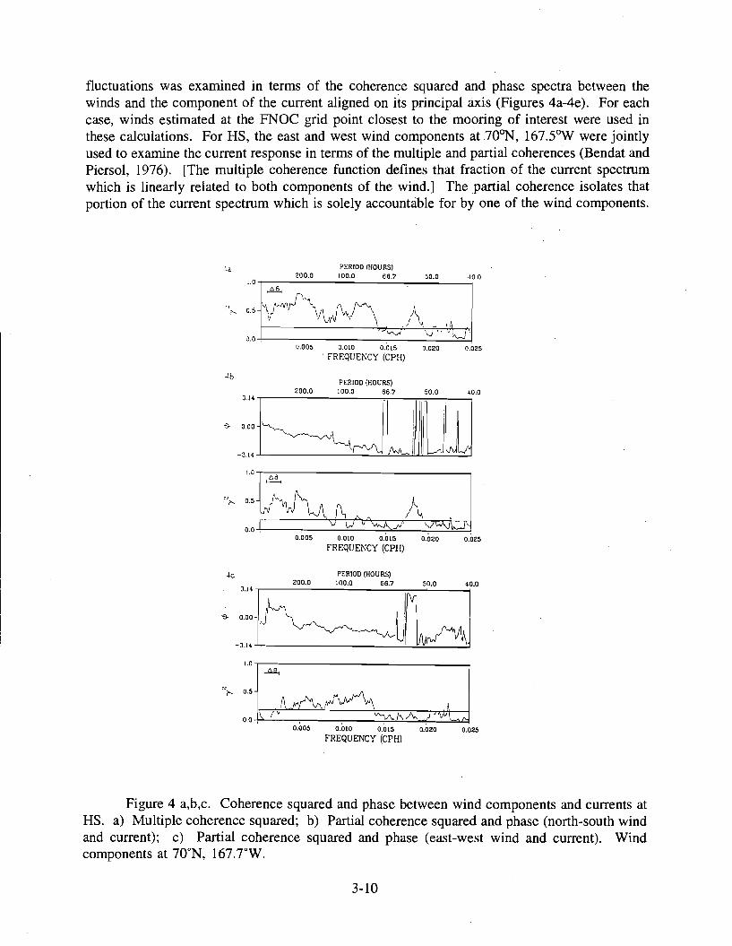
fluctuations was examined in terms of the coherence squared and phase spectra between the winds and the component of the current aligned on its principal axis (Figures 4a-4e). For each case, winds estimated at the FNOC grid point closest to the mooring of interest were used in these calculations. For HS, the east and west wind components at 70oN, 167.5°W were jointly used to examine the current response in terms of the multiple and partial coherences (Bendat and Piersol, 1976). [The multiple coherence function defines that fraction of the current spectrum which is linearly related to both components of the wind.] The partial coherence isolates that portion of the current spectrum which is solely accountable for by one of the wind components.

PERIOD (HOURS) 200.0 100.0 667 50.0 40.0

1.0 ~ r,

" 0.5 .~ 1"-Y1rJ"\ !\ f\ /\,~ 'v Il'rJ V\o, .' . - ,,\

. \rvJ \.J' . u0.0 . 0.005 0.010 0.015 0.020 0.025

. fREQUE1\CY (CPH)

Jb PERIOD (HOURS)

200.0 100.0 66.7 50.0 400 3.14

"S- 0.00

r I~~~l Irl,I ,-I v -3.14

4c PERIOD (HOURS)

~_:+~rLJOO 1.0,-------- ---, ~

0.0 • , . 0.005 0.010 0.Q15 0.020 0.025

FREQUENCY (CPH)

Figure 4 a,b,c. Coherence squared and phase between wind components and currents at HS. a) Multiple coherence squared; b) Partial coherence squared and phase (north-south wind and current); c) Partial coherence squared and phase (east-west wind and current). Wind components at 70oN, l67.TW.

3-10

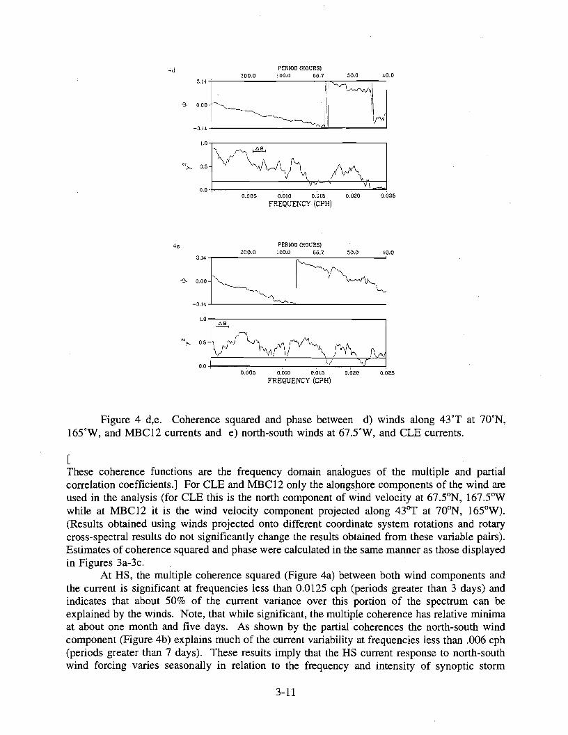
PERIOD (HOURS)4d 200.0 100.0 66.7 50.0 .0.0

3.14 -;---------~;'"';~-----:---;

ill ~I ~ 000 ~ III Iii

~JI' I;v/-3.14 -.I...- __J----:~

1.0...------------------, \J\~

Nr- 0.5 / ~~ /\11\, 0.0 +,__----,-__----,-__V--,-__-,--_\J-'-\~

0.005 0.010 0.015 0.020 0.025

fREQUENCY (CPH)

4e PERIOD (HOURS)

3.14 l 200.0 100.0 ~ 50.0 ••0.0

~-:::~ ~ 1.0...---=----------------, ~

0.0 +-__----,-__...,....-__----,-:.:..-----:----:l'-~

0.005 0.010 0.015 0.020

FREQUENCY (CPH)

Figure 4 d,e. Coherence squared and phase between d) winds along 43°T at 70oN, 165°W, and MBC12 currents and e) north-south winds at 67.5°W, and CLE currents.

[ These coherence functions are the frequency domain analogues of the multiple and partial correlation coefficients.] For CLE and MBC12 only the alongshore components of the wind are used in the analysis (for CLE this is the north component of wind velocity at 67.5°N, 167.5OW while at MBC12 it is the wind velocity component projected along 43o-r' at 70oN, I65°W). (Results obtained using winds projected onto different coordinate system rotations and rotary cross-spectral results do not significantly change the results obtained from these variable pairs). Estimates of coherence squared and phase were calculated in the same manner as those displayed in Figures 3a-3c.

At HS, the multiple coherence squared (Figure 4a) between both wind components and the current is significant at frequencies less than 0.0125 cph (periods greater than 3 days) and indicates that about 50% of the current variance over this portion of the spectrum can be explained by the winds. Note, that while significant, the multiple coherence has relative minima at about one month and five days. As shown by the partial coherences the north-south wind component (Figure 4b) explains much of the current variability at frequencies less than .006 cph (periods greater than 7 days). These results imply that the HS current response to north-south wind forcing varies seasonally in relation to the frequency and intensity of synoptic storm

3-11

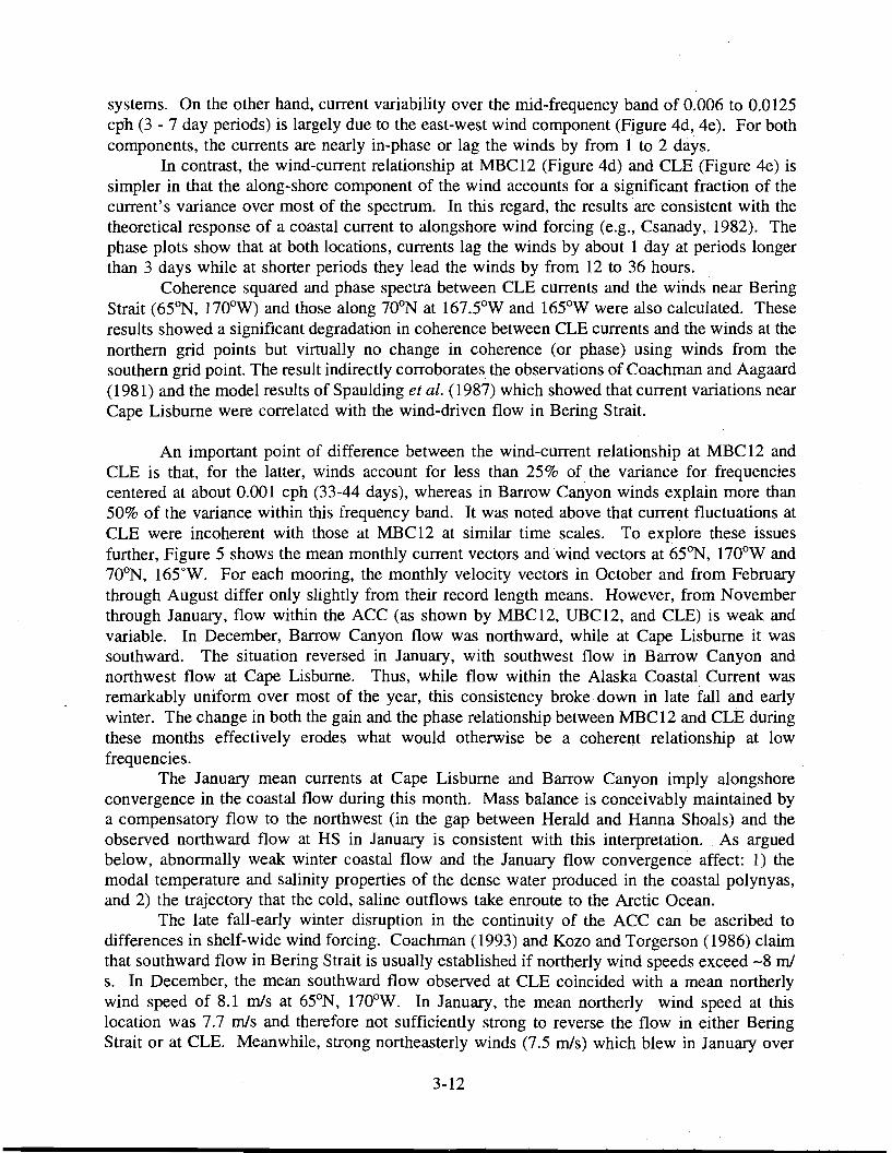
systems. On the other hand, current variability over the mid-frequency band of 0.006 to 0.0125 cph (3 - 7 day periods) is largely due to the east-west wind component (Figure 4d, 4e). For both components, the currents are nearly in-phase or lag the winds by from 1 to 2 days.

In contrast, the wind-current relationship at MBC12 (Figure 4d) and CLE (Figure 4e) is simpler in that the along-shore component of the wind accounts for a significant fraction of the current's variance over most of the spectrum. In this regard, the results are consistent with the theoretical response of a coastal current to alongshore wind forcing (e.g., Csanady, 1982). The phase plots show that at both locations, currents lag the winds by about 1 day at periods longer than 3 days while at shorter periods they lead the winds by from 12 to 36 hours.

Coherence squared and phase spectra between CLE currents and the winds near Bering Strait (65°N, 1700 W) and those along 700 N at 167.5°W and 165°W were also calculated. These results showed a significant degradation in coherence between CLE currents and the winds at the northern grid points but virtually no change in coherence (or phase) using winds from the southern grid point. The result indirectly corroborates the observations of Coachman and Aagaard (1981) and the model results of Spaulding et at. (1987) which showed that current variations near Cape Lisburne were correlated with the wind-driven flow in Bering Strait.

An important point of difference between the wind-current relationship atMBC12 and CLE is that, for the latter, winds account for less than 25% of the variance for frequencies centered at about 0.001 cph (33-44 days), whereas in Barrow Canyon winds explain more than 50% of the variance within this frequency band. It was noted above that current fluctuations at CLE were incoherent with those at MBC12 at similar time scales. To explore these issues further, Figure 5 shows the mean monthly current vectors and wind vectors at 65°N, 1700 Wand 70oN, 165"W. For each mooring, the monthly velocity vectors in October and from February through August differ only slightly from their record length means. However, from November through January, flow within the ACC (as shown by MBCI2, UBCI2, and CLE) is weak and variable. In December, Barrow Canyon flow was northward, while at Cape Lisburne it was southward. The situation reversed in January, with southwest flow in Barrow Canyon and northwest flow at Cape Lisburne. Thus, while flow within the Alaska Coastal Current was remarkably uniform over most of the year, this consistency broke down in late fall and early winter. The change in both the gain and the phase relationship between MBC12 and CLE during these months effectively erodes what would otherwise be a coherent relationship at low frequencies.

The January mean currents at Cape Lisburne and Barrow Canyon imply alongshore convergence in the coastal flow during this month. Mass balance is conceivably maintained by a compensatory flow to the northwest (in the gap between Herald and Hanna Shoals) and the observed northward flow at HS in January is consistent with this interpretation.. As argued below, abnormally weak winter coastal flow and the January flow convergence affect: 1) the modal temperature and salinity properties of the dense water produced in the coastal polynyas, and 2) the trajectory that the cold, saline outflows take enroute to the Arctic Ocean.

The late fall-early winter disruption in the continuity of the ACC can be ascribed to differences in shelf-wide wind forcing. Coachman (1993) and Kozo and Torgerson (1986) claim that southward flow in Bering Strait is usually established if northerly wind speeds exceed -8 m/ s. In December, the mean southward flow observed at CLE coincided with a mean northerly wind speed of 8.1 m/s at 65°N, 170oW. In January, the mean northerly wind speed at this location was 7.7 m/s and therefore not sufficiently strong to reverse the flow in either Bering Strait or at CLE. Meanwhile, strong northeasterly winds (7.5 m/s) which blew in January over

3-12

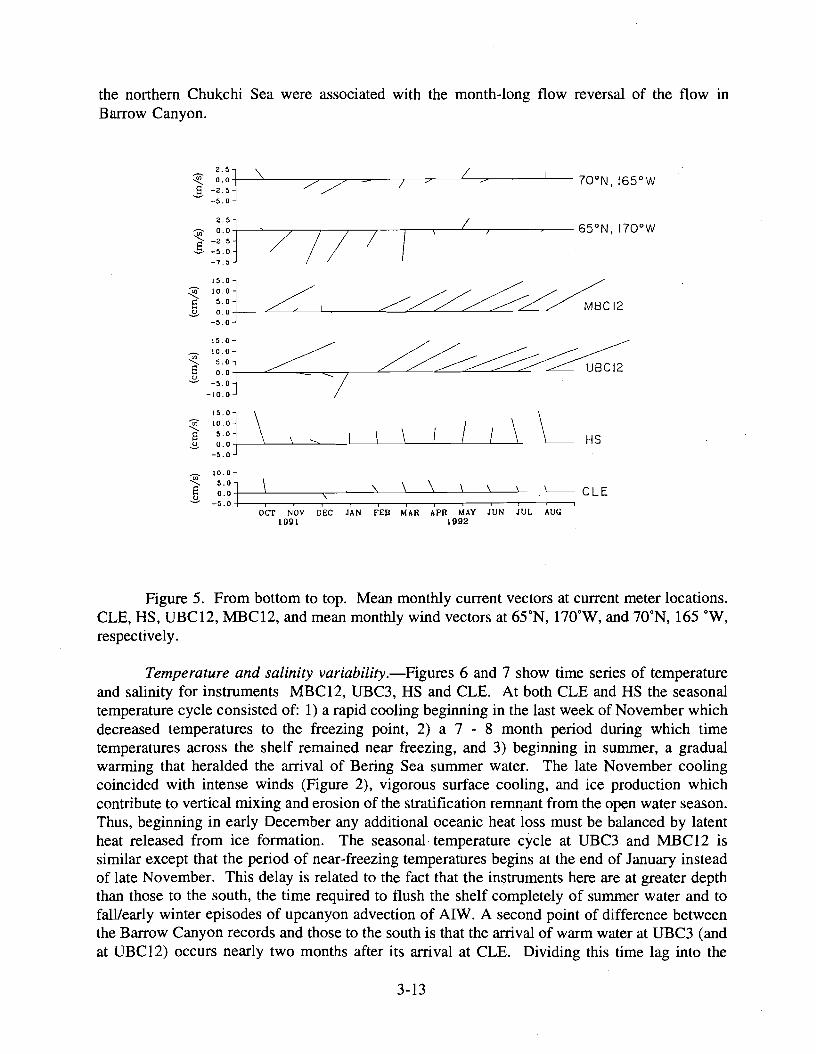
the northern Chukchi Sea were associated with the month-long flow reversal of the flow in Barrow Canyon.

I 7 ;;> ;;>

I 0

'Ul ~: ~ j~'-/---r--/-,-/-r--~/-'----""---------L...---r---~- 65°N, 170 WE -2.5 ~ -5.0

-7.5

~ 10.0

E 5.0 "'- /1$ 0.0

-5.0

15.0 ~ 10.0 ~ 5.0

6 0.0 ~ -5.01 ~/

-10.0

j :mJ-\~>'~----,----------\-----L.---L-/-L..--....I...\.--------l-\_ HS

\ \ \ \

\ CLE , i ii I i i i I I

OCT NOV DEC JAN FEll MAR APR MAY JUN JUL AUG 1091 1992

Figure 5. From bottom to top. Mean monthly current vectors at current meter locations. CLE, HS, UBCI2, MBCI2, and mean monthly wind vectors at 65°N, 170oW, and 70oN, 165 oW, respectively.

Temperature and salinity variability.-Figures 6 and 7 show time series of temperature and salinity for instruments MBCI2, UBC3, HS and CLE. At both CLE and HS the seasonal temperature cycle consisted of: 1) a rapid cooling beginning in the last week of November which decreased temperatures to the freezing point, 2) a 7 - 8 month period during which time temperatures across the shelf remained near freezing, and 3) beginning in summer, a gradual warming that heralded the arrival of Bering Sea summer water. The late November cooling coincided with intense winds (Figure 2), vigorous surface cooling, and ice production which contribute to vertical mixing and erosion of the stratification remnant from the open water season. Thus, beginning in early December any additional oceanic heat loss must be balanced by latent heat released from ice formation. The seasonal temperature cycle at UBC3 and MBC12 is similar except that the period of near-freezing temperatures begins at the end of January instead of late November. This delay is related to the fact that the instruments here are at greater depth than those to the south, the time required to flush the shelf completely of summer water and to fall/early winter episodes of upcanyon advection of AIW. A second point of difference between the Barrow Canyon records and those to the south is that the arrival of warm water at UBC3 (and at UBCI2) occurs nearly two months after its arrival at CLE. Dividing this time lag into the

3-13

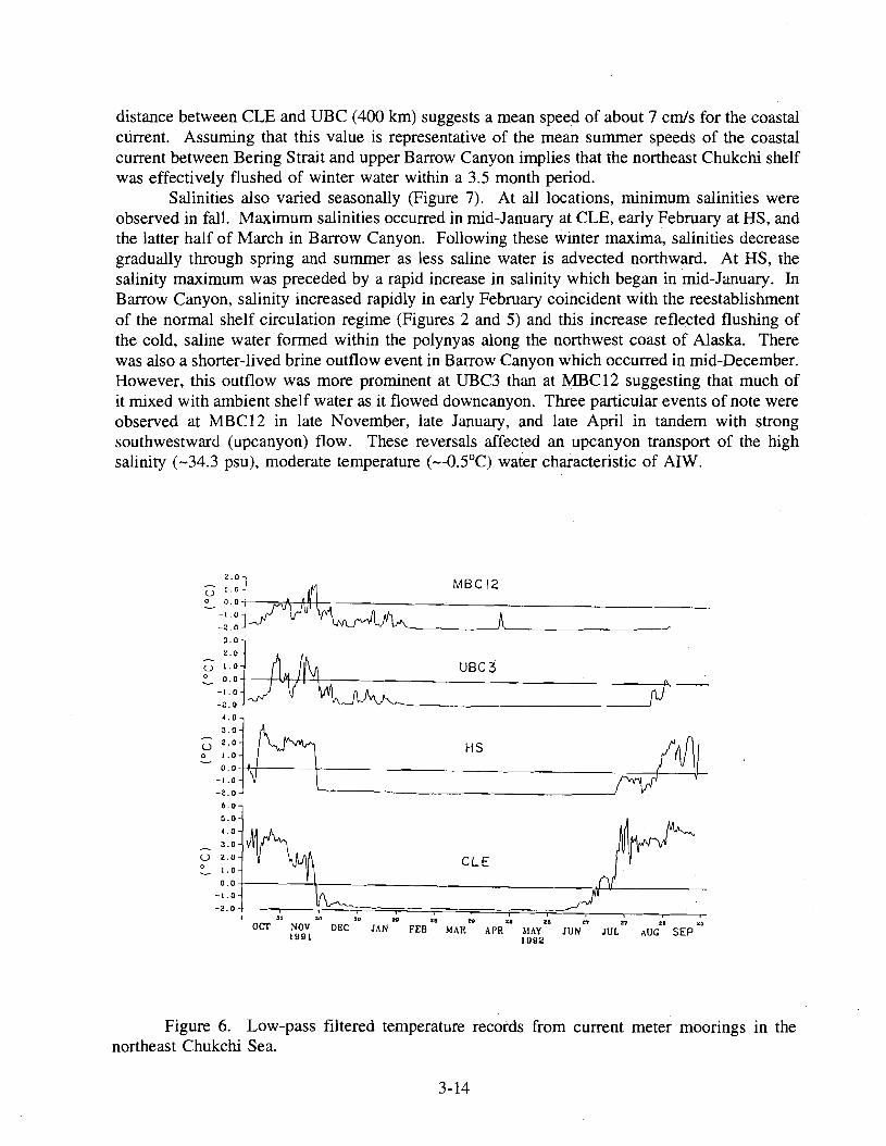
distance between CLE and UBC (400 Ian) suggests a mean speed of about 7 cm/s for the coastal current. Assuming that this value is representative of the mean summer speeds of the coastal current between Bering Strait and upper Barrow Canyon implies that the northeast Chukchi shelf was effectively flushed of winter water within a 3.5 month period.

Salinities also varied seasonally (Figure 7). At all locations, minimum salinities were observed in fall. Maximum salinities occurred in mid-January at CLE, early February at HS, and the latter half of March in Barrow Canyon. Following these winter maxima, salinities decrease gradually through spring and summer as less saline water is advected northward. At HS, the salinity maximum was preceded by a rapid increase in salinity which began in mid-January. In Barrow Canyon, salinity increased rapidly in early February coincident with the reestablishment of the normal shelf circulation regime (Figures 2 and 5) and this increase reflected flushing of the cold, saline water formed within the polynyas along the northwest coast of Alaska. There was also a shorter-lived brine outflow event in Barrow Canyon which occurred in mid-December. However, this outflow was more prominent at UBC3 than at MBC12 suggesting that much of it mixed with ambient shelf water as it flowed downcanyon. Three particular events of note were observed at MBC12 in late November, late January, and late April in tandem with strong southwestward (upcanyon) flow. These reversals affected an upcanyon transport of the high salinity (-34.3 psu), moderate temperature (--0.5°C) water characteristic of AIW.

z.Ol MBC 12U 1.01 ItL--­~ =r:~J7")V'~==~~-A--------

z.o U 1.0 UBC3J'OLt~~ 0.0 A'- "~I--M-- -- ­

=~:~ "'~lJ~ ~ ---,{J

u ~:~j ~ .1t1 nLHS

o =n ~~ -----,rv!~ C.O

5.0

4.0J.O U z.O CLE o 1.0

O.Oi----"t---------------"J-V-- _ -1.0

-z. 0 +---::----::!~=:::==~===;:===;:===;==;=::-::::!...;~--r--_.___---'---; 31 ::Ill 20 U ~o ~8 211 n I • . ­

OCT NOV DEC JAN FEB MAR APR MAY JUN JUL 27 AUG" SEP" 1991 1092

Figure 6. Low-pass filtered temperature records from current meter moorings in the northeast Chukchi Sea.

3-14

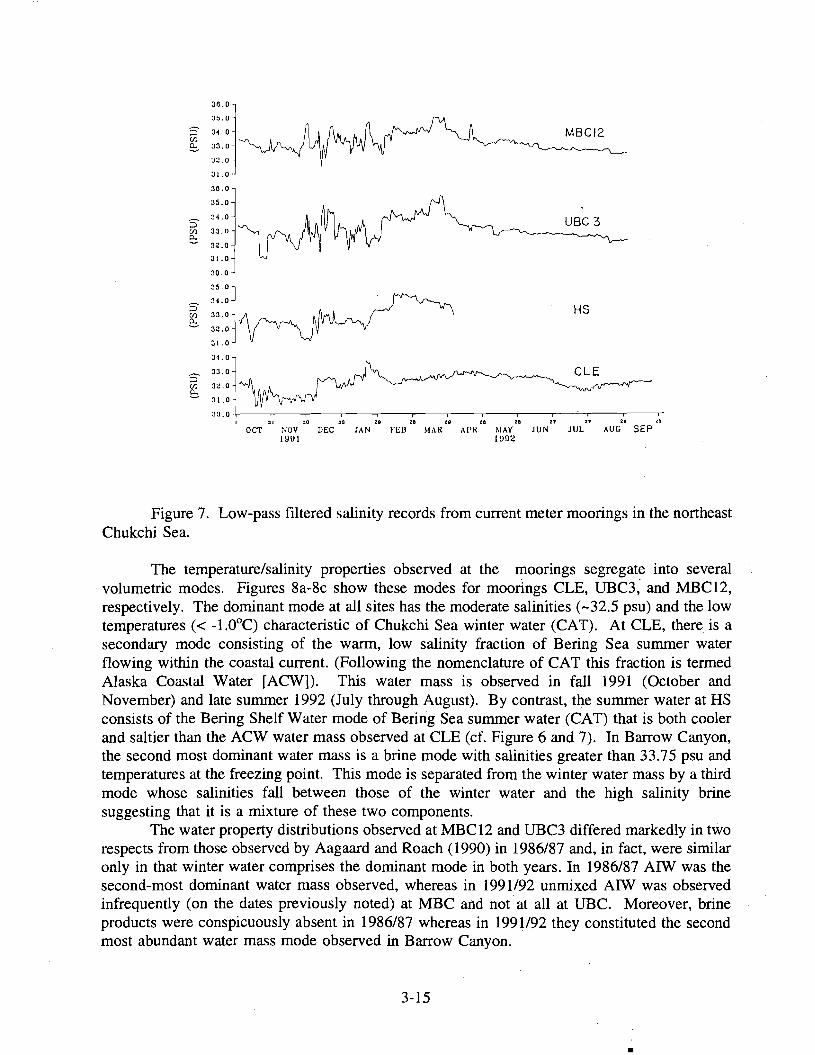
36.6135.0 MBC/2S 3~.0 J ~g ~~:: ~

31.0

36.0

UBC 3

30.0

HS

31.0

S ~:::j Ul 33.0

~ n.o

S ~:::~~. CLE

-----" 28 ll:!)

OCT MAY JUN JUL AUG SEP

g :~:: tJ~-~_'---,-,-----.-'-------,-,------"-------.,-------.,----,,----,,r-~,r_-,' :lQ U U 28 n za 27 27

NOV DEC JAN FED MAR APR 1991 lUD2

Figure 7. Low-pass filtered salinity records from current meter moorings in the northeast Chukchi Sea.

The temperature/salinity properties observed at the moorings segregate into several volumetric modes. Figures 8a-8c show these modes for moorings CLE, UBC3, and MBC12, respectively. The dominant mode at all sites has the moderate salinities (-32.5 psu) and the low temperatures « -l.O°C) characteristic of Chukchi Sea winter water (CAT). At CLE, there is a secondary mode consisting of the warm, low salinity fraction of Bering Sea summer water flowing within the coastal current. (Following the nomenclature of CAT this fraction is termed Alaska Coastal Water [ACW]). This water mass is observed in fall 1991 (October and November) and late summer 1992 (July through August). By contrast, the summer water at HS consists of the Bering Shelf Water mode of Bering Sea summer water (CAT) that is both cooler and saltier than the ACW water mass observed at CLE (cf. Figure 6 and 7). In Barrow Canyon, the second most dominant water mass is a brine mode with salinities greater than 33.75 psu and temperatures at the freezing point. This mode is separated from the winter water mass by a third mode whose salinities fall between those of the winter water and the high salinity brine suggesting that it is a mixture of these two components.

The water property distributions observed at MBC12 and UBC3 differed markedly in two respects from those observed by Aagaard and Roach (1990) in 1986/87 and, in fact, were similar only in that winter water comprises the dominant mode in both years. In 1986/87 AIW was the second-most dominant water mass observed, whereas in 1991/92 unmixed AIW was observed infrequently (on the dates previously noted) at MBC and not' at all at UBC. Moreover, brine products were conspicuously absent in 1986/87 whereas in 1991/92 they constituted the second most abundant water mass mode observed in Barrow Canyon.

3-15

•

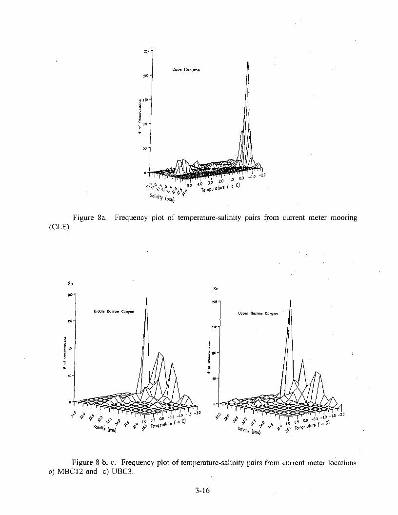
5 10 ·1.5 -20 '0 -.

1.0 0.5 0.0 -. ( 0 C) {>~ -fr" Temperature

250

Cape Usbume

200

• 150 c .9 o i iJ a ~ ,00 o ...

Figure 8a. Frequency plot of temperature-salinity pairs from current meter moormg (CLE).

8b Be

~

~

Middle Borrow Canyon

1~

150

1 jJ,~ it~

,. ~

...•50

50

-20.-05 _1.0 - .,

., 1.0 0.5 0.0 . ( 0 C) " 1" -fr'" .v Temperature

Upper Borrow canyon

Figure 8 b, c. Frequency plot of temperature-salinity pairs from current meter locations b) MBC12 and c) UBC3.

3-16

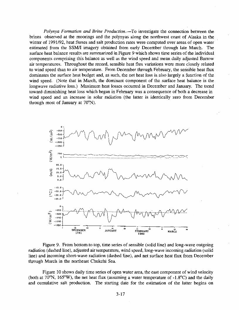
Polynya Formation and Brine Production.-To investigate the connection between the brines observed at the moorings and the polynyas along the northwest coast of Alaska in the winter of 1991/92, heat fluxes and salt production rates were computed over areas of open water estimated from the SSMII imagery obtained from early December through late March. The surface heat balance results are summarized in Figure 9 which shows time series of the individual components comprising this balance as well as the wind speed and mean daily adjusted Barrow air temperatures. Throughout the record, sensible heat flux variations were more closely related to wind speed than to air temperature. From December through February, the sensible heat flux dominates the surface heat budget and, as such, the net heat loss is also largely a function of the wind speed. (Note that in March, the dominant component of the surface heat balance is the longwave radiative loss.) Maximum heat losses occurred in December and January. The trend toward diminishing heat loss which began in February was a consequence of both a decrease in wind speed and an increase in solar radiation (the latter is identically zero from December through most of January at 700 N).

20.0

~ 15.0

B­10.0

5.0

0.0

-10.0

U -20.0

~ -30.0

-40.0

-2~0 ­N E -500 '­3: -750

-1000

-1250

250 I_~_~--"__~~ ~ ~""--~-"""-

o ---------- _. -------- --- a • • __ • • - - - ",.o' ' _.. _ ..__ _. ­

-250 _

N -500

~ -750 ..~~3: -1000-~.~ -1250

I 13 25 e III '0 II 2' a III '0

DECEMBER JANUARY FEBRUARY MARCil 1991 1992

Figure 9. From bottom to top, time series of sensible (solid line) and long-wave outgoing radiation (dashed line), adjusted air temperature, wind speed, long-wave incoming radiation (solid line) and incoming short-wave radiation (dashed line), and net surface heat flux from December through March in the northeast Chukchi Sea.

Figure 10 shows daily time series of open water area, the east component of wind velocity (both at 70oN, 165°W), the net heat flux (assuming a water temperature of -1.8°C) and the daily and cumulative salt production. The starting date for the estimation of the latter begins on

3-17

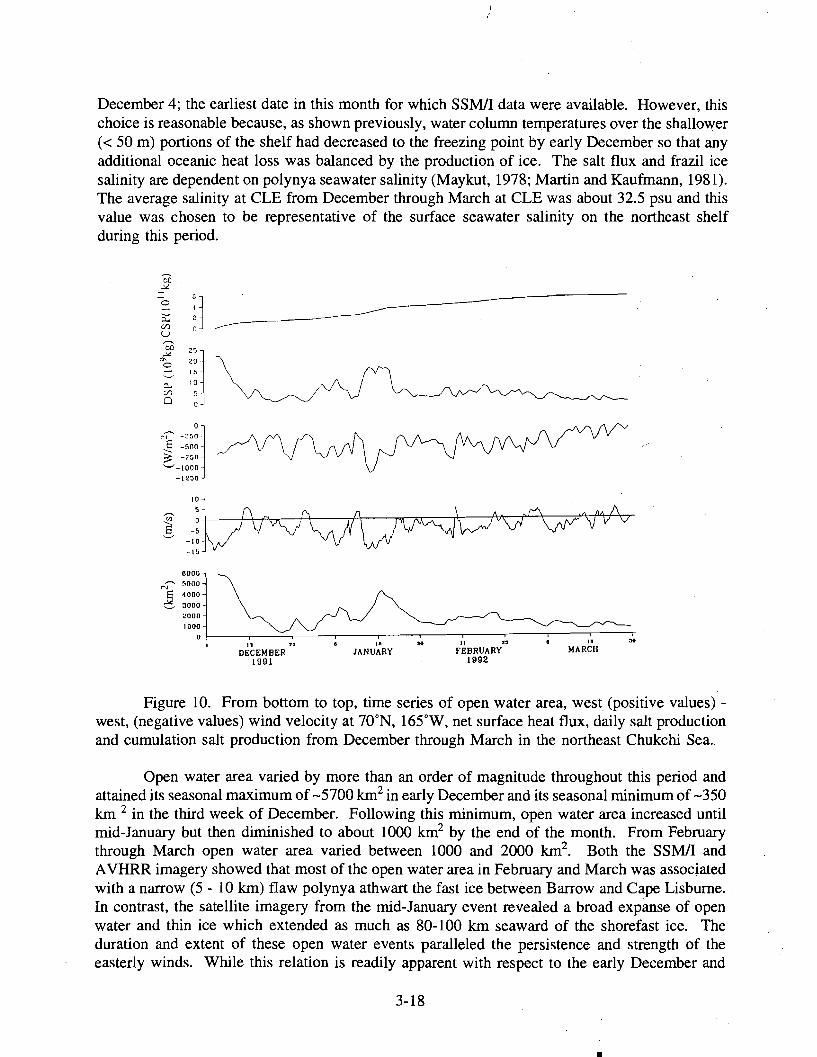
December 4; the earliest date in this month for which SSM/I data were available. However, this choice is reasonable because, as shown previously, water column temperatures over the shallower « 50 m) portions of the shelf had decreased to the freezing point by early December so that any additional oceanic heat loss was balanced by the production of ice. The salt flux and frazil ice salinity are dependent on polynya seawater salinity (Maykut, 1978; Martin and Kaufmann, 1981). The average salinity at CLE from December through March at CLE was about 32.5 psu and this value was chosen to be representative of the surface seawater salinity on the northeast shelf during this period.

n~---------------

r--;-' -:!~o·OJJ§ -500

i3 -700

'-'-1000 -12~O

N"-" 50006000 1 ] ~ooo '-" 3000

2000

1000o-,-------"----..::::::::..--===-------r----,-,--,,--.,-,--,.-,--'---,'--'.-----;:.3~

I D~CEMBER JANU~Ry:lO FEBRUARyl!3 MARCH 1991 1992

Figure 10. From bottom to top, time series of open water area, west (positive values)­west, (negative values) wind velocity at 70oN, 165°W, net surface heat flux, daily salt production and cumulation salt production from December through March in the northeast Chukchi Sea.

Open water area varied by more than an order of magnitude throughout this period and attained its seasonal maximum of -5700 km2 in early December and its seasonal minimum of -350 km 2 in the third week of December. Following this minimum, open water area increased until mid-January but then diminished to about 1000 km2 by the end of the month. From February through March open water area varied between 1000 and 2000 km2

• Both the SSM/I and AVHRR imagery showed that most of the open water area in February and March was associated with a narrow (5 - 10 km) flaw polynya athwart the fast ice between Barrow and Cape Lisburne.. In contrast, the satellite imagery from the mid-January event revealed a broad expanse of open water and thin ice which extended as much as 80-100 km seaward of the shorefast ice. The duration and extent of these open water events paralleled the persistence and strength of the easterly winds. While this relation is readily apparent with respect to the early December and

•

3-18

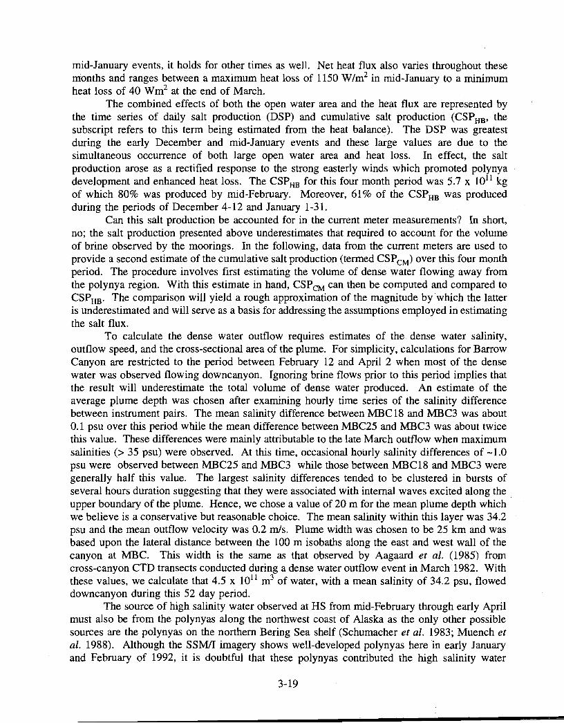
mid-January events, it holds for other times as well. Net heat flux also varies throughout these months and ranges between a maximum heat loss of 1150 W/m2 in mid-January to a minimum heat loss of 40 Wm2 at the end of March.

The combined effects of both the open water area and the heat flux are represented by the time series of daily salt production (DSP) and cumulative salt production (CSPHB, the subscript refers to this term being estimated from the heat balance). The DSP was greatest during the early December and mid-January events and these large values are due to the simultaneous occurrence of both large open water area and heat loss. In effect, the salt production arose as a rectified response to the strong easterly winds which promoted polynya development and enhanced heat loss. The CSPHB for this four month period was 5.7 x 1011 kg of which 80% was produced by mid-February. Moreover, 61% of the CSPHB was produced during the periods of December 4-12 and January 1-31.

Can this salt production be accounted for in the current meter measurements? In short, no; the salt production presented above underestimates that required to account for the volume of brine observed by the moorings. In the following, data from the current meters are used to provide a second estimate of the cumulative salt production (termed CSPCM) over this four month period. The procedure involves first estimating the volume of dense water flowing away from the polynya region. With this estimate in hand, CSPCM can then be computed and compared to CSPHB. The comparison will yield a rough approximation of the magnitude by which the latter is underestimated and will serve as a basis for addressing the assumptions employed in estimating the salt flux.

To calculate the dense water outflow requires estimates of the dense water salinity, outflow speed, and the cross-sectional area of the plume. FOr simplicity, calculations for Barrow Canyon are restricted to the period between February 12 and April 2 when most of the dense water was observed flowing downcanyon. Ignoring brine flows prior to this period implies that the result will underestimate the total volume of dense water produced. An estimate of the average plume depth was chosen after examining hourly time series of the salinity difference between instrument pairs. The mean salinity difference between MBC 18 and MBC3 was about 0.1 psu over this period while the mean difference between MBC25 and MBC3 was about twice this value. These differences were mainly attributable to the late March outflow when maximum salinities (> 35 psu) were observed. At this time, occasional hourly salinity differences of -1.0 psu were observed between MBC25 and MBC3 while those between MBC 18 and MBC3 were generally half this value. The largest salinity differences tended to be clustered in bursts of several hours duration suggesting that they were associated with internal waves excited along the . upper boundary of the plume. Hence, we chose a value of 20 m for the mean plume depth which we believe is a conservative but reasonable choice. The mean salinity within this layer was 34.2 psu and the mean outflow velocity was 0.2 m/s. Plume width was chosen to be 25 km and was based upon the lateral distance between the 100 m isobaths along the east and west wall of the canyon at MBC. This width is the same as that observed by Aagaard et al. (1985) from cross-canyon CTD transects conducted during a dense water outflow event in March ·1982.. With these values, we calculate that 4.5 x 1011 m3 of water, with a mean salinity of 34.2 psu, flowed downcanyon during this 52 day period.

The source of high salinity water observed at HS from mid-February through early April must also be from the polynyas along the northwest coast of Alaska as the only other possible sources are the polynyas on the northern Bering Sea shelf (Schumacher et ai. 1983; Muench et ai. 1988). Although the SSMII imagery shows well-developed polynyas here in early January and February of 1992, it is doubtful that these polynyas contributed the high salinity water

3-19

observed at HS for a number of reasons. Chief among these are that: 1) there was no indication of northward advection of high salinity water at either CLE or CLWand 2) for this saline water to arrive at HS in mid-February implies a mean northward flow of 0.3 m/s and currents of this magnitude contradict the mean January flow estimated at CLE. Next, we assumed that the dense water observed at HS reflects a broader outflow into the north central Chukchi Sea through the gap between Herald and Hanna Shoal. The assumed plume width is 250 km (the dis~ance

between the 40 m isobath bounding Hanna and Herald Shoal) and its height above sea-bottom was chosen to be 5 m. This depth is consistent with the 3 meter height of the instrument above the bottom and with the salinity cross-section from March 1982 (Aagaard et aI. 1985) which shows the 34 psu isohaline extending seaward from the coast within a thin bottom layer. Plume speed was chosen to be 0.02 m/s and was determined as follows. First, the arrival of the high salinity water at HS in February lags by two months the December polynya event and by one month the January polynya opening. As the mooring was approximately 100 km west of the open water/thin ice boundary as determined from January AVHRR imagery a northwesterly velocity of about 0.01-0.03 m/s is inferred. A second estimate was derived by assuming that the mean January onshelf flow at UBC12 of 0.13 m/s approximates the average cross-sectional current speed at the head of Barrow Canyon where the width is about 20 km and the water depth is about 75 m. These numbers yield a southwestward transport of -2x 105 m3/s. This transport was assumed to be balanced by a northwesterly flow between Hanna and Herald Shoals, because the Cape Lisburne moorings show negligible transport in January across this section. The depth· between these shoals is about 45 m and, in conjunction with the channel's width, implies a mean speed of 0.02 m-s· l

. Both estimates are consistent with one another and with the numerical model results of Spaulding et aI. (1987; their Figure l2b) for this shelfs circulation when forced by easterly winds. With these values, we calculate that 1.2 x 1011 m3 of water, with a mean salinity of 33.9 psu, flowed through this gap during the 56-day period from February 10 and April 5.

The CSPCM required to balance these outflows follows from Alfultis and Martin (1987) and, after rearranging their equation 8, is estimated accordingly:

where Q dw is the salinity of the dense water outflow, Vdwis the volume of dense water, Ssw =32.5 psu, is the initial polynya seawater salinity, and Pdw is the density of Sdw at the freezing point. (The CSPCM computed in this way can be very sensitive to the choice of either. Sdw or Ssw' However, changes in Sdw will be buffered by changes in Vdw due to compensatory changes in plume depth, the vertically averaged plume speed, and the duration of the dense water outflow.) Performing this calculation for the two outflows and summing the results yields a CSPCM of 9.6 x 1011 kg. Of this total, 82% is required to balance the Barrow Canyon outflow. Hence, CSPCM is (at least) about 70% greater than that estimated from the surface heat balance approach.

To overcome this deficit would require an additional average daily heat loss of 350 W/m2

over the December to March period. Relative to the sensible heat flux term, the magnitudes of the other terms contributing to the surface heat balance are small and are either of the same magnitude or smaller than the additional heat loss required. Thus it seems unlikely that these could be the source of the discrepancy. The sensible heat flux could be underestimated if wind speeds or the transfer coefficient are too low or if air temperatures are too warm. Aagaard et al. (1990) compared 6-hourly wind speeds estimated from the FNOC surface pressure fields with those measured at coastal weather stations along the Chukchi and Beaufort coasts and found that

3-20

mean wind speeds differ by less than 1 mlsl although the FNOC wind estimates are consistently higher. The air temperatures used in the heat balance equation were essentially obtained upwind of the polynya during such events and therefore, if biased, are more likely too cold rather than too warm (Pease, 1987; Sverdrup, 1933). The transfer coefficient used (2 x 10-3

), while a subject of considerable uncertainty, falls well within the parametrized values (Pease, 1987). In short, in order to increase the magnitude of the sensible heat loss term to satisfy the salt deficit would require unrealistic changes in wind speeds, air temperatures, and/or the heat transfer coefficient.

Nor can the discrepancy be satisfied by changing the seawater salinity which in our calculation of the DSP was assumed to be constant. A reasonable argument could be advanced that due to the near-stagnant shelf circulation of December and January polynya salinities increased over time. However, in our formulation the relationship between salt flux and seawater salinity is linear, hence even large changes in Ssw will not significantly improve our results. For· example, increasing the salinity by 8% (from 32.5 to 35 psu) increases CSPHB by the same percentage.

The difference might result from the fact that our calculation ignores the salt flux contributed by ice growth in areas of thin ice. Because of the insulating effect of the sea-ice cover oceanic heat loss decays rapidly with ice thickness. For example, according to Maykut (1978) the oceanic heat losses through ice thicknesses of 0.1, 0.2, or 1 mare 40%,25%, and 8% respectively of the heat loss through open water. To estimate the additional salt production that might be contributed by ice production in areas of thin ice we assumed that the spatially averaged ice thickness inshore of the 40 m isobath and between 68°N and 700 N is 1 m. The area of this region is 45,000 km2 and it lies within the thin ice boundary seen in the January AVHRR imagery. The average net daily heat loss (over open water) from December through March was 425 W/m2 which corresponds to a oceanic heat loss of 30 W/m2 over 1 m of ice. Thus ice growth in this region could contribute an additional 9 x lOll kg of salt throughout this period and this production is more than sufficient to satisfy the estimated salt deficit.

DISCUSSION

While the extensive ice-cover in the fall of 1991 prevented us from achieving several of the original objectives, the modified program did provide new insights into the circulation over the central shelf and permits a comparison with previous observations of the coastal current and of dense water production on this shelf.

The current meter results from Herald Shoal indicated steady northward flow in all months of the year. In contrast, CAT inferred a southeasterly flow here and through the gap formed by these shallows and suggested that part of this flow joined the coastal current before draining through Barrow Canyon. However, summer and fall ice maps for the Chukchi Sea frequently show a northward indentation in the ice-edge to the north and east of Herald Shoal which is presumably a consequence of enhanced melting by warm water advection from the Bering Sea (Paquette and Bourke, 1981). The perennial nature of this ice-edge feature was, in fact, well-known in the 19th century when it was used as a rendezvous point by whalers venturing to and from their hunting grounds in the Chukchi Sea (Bockstoce, 1986). Hence, the earlier ice-edge observations tend to corroborate the mooring results and suggest that the mean northward flow observed here is a persistent feature of the shelf circulation. Because this flow consists mainly of Bering Shelf Water rather than Alaska Coastal Water, its organic carbon load is richer than that of the coastal current to the east (Walsh et ai. 1989). Indeed, striking differences are seen between the vertical profiles of fluorescence (Figure 11) from CTD stations

3-21

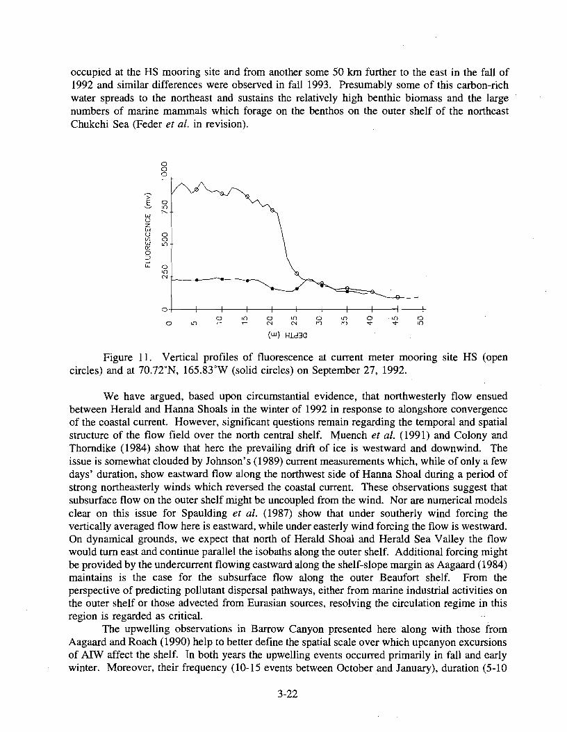
occupied at the HS mooring site and from another some 50 km further to the east in the fall of 1992 and similar differences were observed in fall 1993. Presumably some of this carbon-rich water spreads to the northeast and sustains the relatively high benthic biomass and the large numbers of marine mammals which forage on the benthos on the outer shelf of the northeast Chukchi Sea (Feder et ai. in revision).

0 0 0

>',5, 0

ll)

r--­w u z w u 0 U1 0 W ll)oc 0 ::J ...J u.. 0

ll)

N

o4--+---+---+----+---+---+---!-----1--f----+ o o ll) o N n ll)o n

(w) Hld30

Figure 11. Vertical profiles of fluorescence at current meter mooring site HS (open circles) and at 70.72°N, 165.83°W (solid circles) on September 27, 1992.

We have argued, based upon circumstantial evidence, that northwesterly flow ensued between Herald and Hanna Shoals in the winter of 1992 in response to alongshore convergence of the coastal current. However, significant questions remain regarding the temporal and spatial structure of the flow field over the north central shelf. Muench et al. (1991) and Colony and Thorndike (1984) show that here the prevailing drift of ice is westward and downwind. The issue is somewhat clouded by Johnson's (1989) current measurements which, while of only a few days' duration, show eastward flow along the northwest side of Hanna Shoal during a period of strong northeasterly winds which reversed the coastal current. These observations suggest that subsurface flow on the outer shelf might be uncoupled from the wind. Nor are numerical models clear on this issue for Spaulding et al. (1987) show that under southerly wind forcing the vertically averaged flow here is eastward, while under easterly wind forcing the flow is westward. On dynamical grounds, we expect that north of Herald Shoal and Herald Sea Valley the flow would tum east and continue parallel the isobaths along the outer shelf. Additional forcing might be provided by the undercurrent flowing eastward along the shelf-slope margin as Aagaard (1984) maintains is the case for the subsurface flow along the outer Beaufort shelf. From the perspective of predicting pollutant dispersal pathways, either from marine industrial activities on the outer shelf or those advected from Eurasian sources, resolving the circulation regime in this region is regarded as critical.

The upwelling observations in Barrow Canyon presented here along with those from Aagaard and Roach (1990) help to better define the spatial scale over which upcanyon excursions of AIW affect the shelf. In both years the upwelling events occurred primarily in fall and early winter. Moreover, their frequency (10-15 events between October and January), duration (5-10

3-22

days), and intensity (mean speeds of about 0.5 mfs) were similar in both years. The persistence and intensity of these reversals is such that water from along the continental slope could easily traverse the 250 kIn longitudinal extent of the canyon. Yet observations of AIW on the shallower reaches of the shelf are extremely rare (Bourke and Paquette, 1976). Aagaard and Roach (1990) observed that the outflows, which immediately followed upcanyon intrusions of AIW, were a blend of shelf water and AIW and therefore, they concluded that significant mixing occurred upcanyon from their moorings. Our moorings detected unmixed AIW very infrequently at the mid-canyon site and not at all at the head ofthe canyon. Although the two data sets come from different years, collectively they suggest that much of this mixing must occur in the lower half of the canyon thereby diluting much of the AIW before it reaches the upper canyon and the shallower portions of the shelf.

This data set, those described by Aagaard and Roach (1990) and Aagaard et al. (1990) for 1986/87, and that presented by Aagaard (1988) for 1981/82 allow several comparative statements to be drawn regarding interannual differences in flow on the northeast Chukchi shelf. The velocity records from Barrow Canyon for these years are generally similar, differing primarily from late fall through early winter. For example, the records from 1981/82 differ from the other two years in that few current reversals occurred after November in Barrow Canyon. If these reversals are driven by wind-forced shelf waves propagating along the continental slope, then the 1981/82 results imply that these were less energetic in that year compared to either 1986/87 or 1991/92. Moreover, Aagaard's (1988) records from offshore of Cape Lisburne show relatively steady year-round flow. Thus it would seem that the alongshore convergence of the coastal current that was seen in the winter of 1991/92 was not a feature of the shelf circulation in the winter of 1981/82. In 1986/87, the Barrow Canyon records suggest that, beginning in mid-December, currents reversed across the shelf for about three weeks but by early January they were once again strongly northeastward. Thus, the data from these earlier years suggests nothing comparable to the period of prolonged weak flow as observed from November 1991 through January 1992. However, given the small number of data sets available it would be premature to determine which, if any, of these winters is typical.

Because of the weak mid-winter circulation, the residence time of a water parcel on the shelf and in the polynyas was prolonged. Consequently, brines accumulated within the polynya and increased a water parcel's salinity to a greater extent than would have been possible if the parcel was advected rapidly through the region. We maintain that because weak flow prevailed over the northern Bering shelf as well, this effect enhanced shelf salinities in this region as well.

We note that there are several significant consequences associated with diversion of coastal water to the northwest. First, such a flow provides a mechanism by which pollutants from the coastal zone can be dispersed onto the north central shelf. Second, as mixing with ambient shelf water alters the water mass properties of the shelf-produced brines flowing into the Arctic Ocean, different mixing regimes are expected depending upon the flow path. The flow trajectory will also affect the biogeochemical properties of the dense water as these will be influenced by exchange with the seabed and the time in which the plume is in contact with the bottom. Third, the outflowing dense water will affect the momentum balance along the continental slope and the nature of this forcing will depend, in part, upon whether the outflow is spread over a broad area or confined to a narrow channel such as Barrow Canyon (Shaw and Csanady, 1983).

There are also differences among these years in polynya extent, the duration of open water events, and the cumulative salt production. As the regions analyzed by CM differ somewhat from those considered here a direct comparison cannot be drawn at this time. However, CM do

3-23

show that the CSPHB in 1981/82 was twice that of 1986/87 and these differences are largely due to' diminished open water area in 1986/87. Tentatively, it appears that the CSPHB and open water area of 1991/92 falls between the values observed in these earlier years. Preliminary examination of the wind records suggest that differences in polynya size as well as the shelf circulation relate to interannual differences in the large-scale wind-forcing over the Chukchi Sea and the northern Bering Sea. Additional analyses along these lines are currently underway.

SUMMARY

Five current meter moorings were deployed in the northeast Chukchi Sea from October 1991 through September 1992. Four were deployed in the Alaska Coastal Current; two offshore of Cape Lisburne and two in Barrow Canyon. A fifth mooring was deployed in the central Chukchi Sea approximately 250 krn west of Barrow Canyon.

The results show that current variations were: 1) spatially coherent throughout the northeast Chukchi Sea and 2) significantly coherent with the local wind field. However, currents offshore of Cape Lisburne were more coherent with winds over the northern Bering shelf than they were with winds over the northern Chukchi Sea suggesting that here the coastal current's dynamics are, in part, tied to sea-level adjustments associated with wind-driven transport variations in Bering Strait.

The data depict a shelf circulation which is remarkably steady and swift in most months of the year. However, from November 1991 through January 1992, flow on the northeast shelf was nearly stagnant and the along-shore coherence of the coastal current broke down. Disruption of the coastal flow occurred simultaneously with the formation of polynyas along Alaska's northwest coast which enhanced shelf salinity due to brine rejection from growing ice. Hence, the formation of cold saline water is viewed as a rectified response of the ice and ocean to strong northeasterly winds which: 1) favored polynya development, 2) enhanced sensible heat loss, and 3) led to weak shelf circulation. The salinization effect was enhanced by the weak circulation which effectively increased the residence time of water parcels within the polynyas thereby allowing salinity to increase to a greater extent than would be expected if. strong flow had persisted. In January, basin-scale differences in winds forced alongshore convergence within the coastal current because strong winds reversed the flow in Barrow Canyon but not in Bering Strait or offshore Cape Lisburne.

Most of the cold and saline dense water formed in these polynyas entered the Arctic Ocean through Barrow Canyon after the normal shelf circulation was reestablished in February. However, because of convergence within the coastal current in January, a substantial portion of the dense water drained to the northwest; through the channel between Herald and Hanna Shoal.

Estimates of total salt produced from ice formed in the polynyas are at least a factor of two smaller than salt flux estimates based upon the current meter observations. However, it seems plausible that additional salt produced in areas of thin ice, which are noteasIly ascertained by the satellite imagery, would be more than sufficient to remove the observed discrepancy.

3-24