Embed Size (px)
Citation preview

InstitutLeibniz-Institut für Wirtschaftsforschung
an der Universität München e.V.
ifo Beiträgezur Wirtschaftsforschung74
Five Essays on International Trade, Factor Flows, and the Gains from Globalization
Inga Heiland

InstitutLeibniz-Institut für Wirtschaftsforschung
an der Universität München e.V.
ifo Beiträgezur Wirtschaftsforschung74
Five Essays on International Trade, Factor Flows, and the Gains from Globalization
Inga Heiland
Herausgeber der Reihe: Clemens FuestSchriftleitung: Chang Woon Nam

Bibliografische Information der Deutschen Nationalbibliothek
Die Deutsche Nationalbibliothek verzeichnet diese Publikation in der Deutschen Nationalbibliografie; detaillierte bibliografische
Daten sind im Internet über http://dnb.d-nb.de
abrufbar
ISBN-13: 978-3-95942-024-2
Alle Rechte, insbesondere das der Übersetzung in fremde Sprachen, vorbehalten. Ohne ausdrückliche Genehmigung des Verlags ist es auch nicht gestattet, dieses Buch oder Teile daraus auf photomechanischem Wege (Photokopie, Mikrokopie)
oder auf andere Art zu vervielfältigen. © ifo Institut, München 2017
Druck: ifo Institut, München
ifo Institut im Internet: http://www.cesifo-group.de

Preface
This volume was prepared by Inga Heiland while she was working at the Ifo Institute.It was completed in July 2016 and accepted as a doctoral thesis by the Department ofEconomics at the University of Munich. It comprises five chapters addressing one or moreaspects of international trade and factor movements, including trade in goods, trade invalue added, international movement of labor and capital, and trade in risk. All chaptersaim to contribute to our understanding of the economic gains from globalization in itsvarious forms. Thereby, they touch more or less explicitly on the issues of the determinantsof the pattern of trade, factor flows, and production, as well as the role of barriers to theinternational exchange of goods and factors. From a methodological point of view, allchapters share a strong emphasis on general equilibrium analysis, and those chapters thatare accompanied by an empirical analysis rely primarily on structural estimation.
Chapters 1 and 2 are concerned with the interaction of goods and factor markets indetermining the pattern of trade and factor movements and in shaping the welfare effectsof globalization. Chapter 1 addresses trade in goods and capital flows. It analyzes the rolethat cross-border trade in goods and assets play in sharing risk among countries, and itdescribes how the pattern of these flows is jointly determined as an outcome of individualdecisions taken by investors maximizing utility and firms maximizing shareholder value.In Chapter 2 the focus lies on the interplay between trade and labor markets. In a purelytheoretical analysis, well-established results on the gains from trade derived from modelswith product differentiation are revisited in a framework that includes skill differentiationin the labor force. Chapters 3, 4, and 5 are concerned with the quantification of the gainsfrom trade liberalization. The analyses build on and extend current work in the fields ofthe “New Quantitative Trade Theory” (NQTT). Chapter 3 analyzes the effects of tradeliberalization in the presence of globally fragmented production chains. Chapter 4 buildson and extends the model framework used in Chapter 3 to quantify the global effectsof the Transatlantic Trade and Investment Partnership (TTIP), which is the subject ofcurrent negotiations between the United States and the European Union. Chapter 5 aimsfor a methodological contribution to the NQTT. It discusses the implications of parameteruncertainty for model-based counterfactual analysis with estimated structural parameters.
Keywords: International Trade, International Investment, Asset Pricing, StructuralGravity, Two-way Migration, Heterogeneous Workers, Trade in ValueAdded, Production Networks, China’s WTO entry, Preferential TradeAgreements, TTIP, Bootstrap
JEL-No: C54, F12, F13, F14, F15, F16, F17, F22, F36, F44, G11, J24


Acknowledgements
I owe thanks to all those who supported me during the years when this dissertationwas written.
First and foremost, I want to thank Gabriel Felbermayr for supervising my disserta-tion. His continous support and invaluable advice during my time as a PhD student atIfo laid the groundwork on which my dissertation research evolved, culminating in thesuccessful completion of this thesis. The frequent exchange of ideas with Gabriel andour collaboration in joint projects induced many fruitful learning processes from which Iam benefiting to date. I am also indebted to Carsten Eckel for co-supervising my the-sis, as well as for invaluable comments and challenging questions along the way to itscompletion. I am equally indebted to Wolfgang Keller for being part of my dissertationcommittee, for his advice, and for the invitation to join the trade group at the Universityof Colorado Boulder in the Fall of 2015. In 2014, I had the opportunity to spend a year atStanford University and I would like to thank Kalina Manova for inviting me. Being partof the trade group at Stanford enabled me to take advantage of the outstanding researchenvironment and the exchange with scholars at Stanford University, which significantlycontributed to my dissertation research.
I am grateful to Wilhelm Kohler for the fruitful collaboration in joint projects. Iwould also like to thank him for his passionate teaching of international economics at theUniversity of Tuebingen, that I had the opportunity to enjoy in the early stages of myacademic life, and which opened up the path to academic research for me. A significantpart of my dissertation research evolved out of joint work with Rahel Aichele, whom Iwould like to thank for the great ideas and effort that went into our joint projects.
During my time at Ifo, I benefited greatly from scholarly advice and personal supportof many colleagues, fellow PhD students, and administrative staff. Special thanks go toSybille Lehwald, Erdal Yalcin, Michele Battisti, Christiane Harms, and Anna Gumpert,although many more would deserve to be mentioned. Moreover, I am thankful for JanHeiland’s advice on tough math and programming problems. Finally, I am inexpressiblygrateful for my family’s and my partner’s unconditional love and support at all times.


Five Essays on International Trade, FactorFlows, and the Gains from Globalization
Inaugural-Dissertationzur Erlangung des Grades Doctor oeconomiae publicae (Dr. oec. publ.)
an der Ludwig-Maximilians-Universität München
2016
vorgelegt vonInga Heiland
Referent: Prof. Gabriel Felbermayr, PhDKorreferent: Prof. Dr. Carsten EckelPromotionsabschlussberatung: 16. November 2016


Contents
Introduction 1
1 Global Risk Sharing Through Trade in Goods and Assets: Theory andEvidence 91.1 Introduction . . . . . . . . . . . . . . . . . . . . . . . . . . . . . . . . . . 91.2 Related Literature . . . . . . . . . . . . . . . . . . . . . . . . . . . . . . . 121.3 Theory . . . . . . . . . . . . . . . . . . . . . . . . . . . . . . . . . . . . . . 15
1.3.1 Utility, Consumption, and Investment . . . . . . . . . . . . . . . . . 151.3.2 Firm Behavior . . . . . . . . . . . . . . . . . . . . . . . . . . . . . . 191.3.3 Model Closure . . . . . . . . . . . . . . . . . . . . . . . . . . . . . . 231.3.4 Equilibrium Risk Premia and the Risk-Return Tradeoff . . . . . . . 29
1.4 Empirics . . . . . . . . . . . . . . . . . . . . . . . . . . . . . . . . . . . . . 321.4.1 Estimating λ . . . . . . . . . . . . . . . . . . . . . . . . . . . . . . 321.4.2 Estimating λs for the U.S. Financial Market . . . . . . . . . . . . . 331.4.3 Testing the Relevance of Risk Premia in the Gravity Model . . . . . 36
1.5 Conclusion . . . . . . . . . . . . . . . . . . . . . . . . . . . . . . . . . . . . 45Appendix A.1 . . . . . . . . . . . . . . . . . . . . . . . . . . . . . . . . . . . . . 47
2 Heterogeneous Workers, Trade, and Migration 632.1 Introduction . . . . . . . . . . . . . . . . . . . . . . . . . . . . . . . . . . . 632.2 The Modeling Framework . . . . . . . . . . . . . . . . . . . . . . . . . . . 69
2.2.1 Price and Wage Setting with Worker Heterogeneity . . . . . . . . . 702.2.2 Entry Decision and the Equilibrium Distance Pattern . . . . . . . . 782.2.3 Autarky Equilibrium . . . . . . . . . . . . . . . . . . . . . . . . . . 822.2.4 Distortions . . . . . . . . . . . . . . . . . . . . . . . . . . . . . . . 85
2.3 Symmetric Trading Equilibrium . . . . . . . . . . . . . . . . . . . . . . . . 862.3.1 Free Trade . . . . . . . . . . . . . . . . . . . . . . . . . . . . . . . . 872.3.2 Costly Trade and Piecemeal Trade Liberalization . . . . . . . . . . 88
2.4 Migration . . . . . . . . . . . . . . . . . . . . . . . . . . . . . . . . . . . . 922.4.1 Modeling Migration . . . . . . . . . . . . . . . . . . . . . . . . . . . 92

vi
2.4.2 Labor Supply with Integrated Labor Markets . . . . . . . . . . . . 932.4.3 The “Trade cum Migration” Equilibrium . . . . . . . . . . . . . . . 96
2.5 Conclusion . . . . . . . . . . . . . . . . . . . . . . . . . . . . . . . . . . . . 100Appendix A.2 . . . . . . . . . . . . . . . . . . . . . . . . . . . . . . . . . . . . . 102
3 Where is the Value Added? Trade Liberalization and ProductionNetworks 1293.1 Introduction . . . . . . . . . . . . . . . . . . . . . . . . . . . . . . . . . . 1293.2 A Model for Trade in Value Added . . . . . . . . . . . . . . . . . . . . . . 134
3.2.1 Production and Gross Exports . . . . . . . . . . . . . . . . . . . . . 1343.2.2 General Equilibrium . . . . . . . . . . . . . . . . . . . . . . . . . . 1363.2.3 Comparative Statics in General Equilibrium . . . . . . . . . . . . . 1373.2.4 Value Added Trade . . . . . . . . . . . . . . . . . . . . . . . . . . . 1383.2.5 Gravity in Value Added . . . . . . . . . . . . . . . . . . . . . . . . 1413.2.6 Decomposition of Exports into Value Added Components . . . . . . 145
3.3 Production Networks . . . . . . . . . . . . . . . . . . . . . . . . . . . . . . 1463.3.1 Supply Networks . . . . . . . . . . . . . . . . . . . . . . . . . . . . 1473.3.2 Demand Networks . . . . . . . . . . . . . . . . . . . . . . . . . . . 151
3.4 Data and Parameter Identification . . . . . . . . . . . . . . . . . . . . . . 1543.4.1 Data Sources . . . . . . . . . . . . . . . . . . . . . . . . . . . . . . 1553.4.2 Identification of Sectoral Productivity Dispersion . . . . . . . . . . 1553.4.3 Expenditure and Cost Shares . . . . . . . . . . . . . . . . . . . . . 157
3.5 Counterfactual Analysis: China’s WTO Accession . . . . . . . . . . . . . . 1603.5.1 Developments in China’s Export Composition and Bilateral Value
Added Trade Relationships in the 2000s . . . . . . . . . . . . . . . 1603.5.2 China’s Accession to the WTO in 2001 . . . . . . . . . . . . . . . . 1623.5.3 Results: The Effect of China’s WTO Entry . . . . . . . . . . . . . 164
3.6 Conclusion . . . . . . . . . . . . . . . . . . . . . . . . . . . . . . . . . . . 175
4 Going Deep: The Trade and Welfare Effects of TTIP 1774.1 Introduction . . . . . . . . . . . . . . . . . . . . . . . . . . . . . . . . . . 1774.2 Methodology . . . . . . . . . . . . . . . . . . . . . . . . . . . . . . . . . . 181
4.2.1 The Gravity Model . . . . . . . . . . . . . . . . . . . . . . . . . . . 1814.2.2 Comparative Statics in General Equilibrium . . . . . . . . . . . . . 183
4.3 Data and Parameter Identification . . . . . . . . . . . . . . . . . . . . . . 1844.3.1 Data Sources . . . . . . . . . . . . . . . . . . . . . . . . . . . . . . 1844.3.2 Expenditure and Cost Shares . . . . . . . . . . . . . . . . . . . . . 185

vii
4.3.3 Identification of Trade Cost Parameters . . . . . . . . . . . . . . . . 1854.4 Simulation Results: Trade and Welfare Effects of the TTIP . . . . . . . . 193
4.4.1 Cross-industry facts for the EU and the United States . . . . . . . . 1944.4.2 Global Trade Effects of the TTIP . . . . . . . . . . . . . . . . . . . 1974.4.3 Bilateral Trade Effects of the TTIP . . . . . . . . . . . . . . . . . . 1984.4.4 Sectoral Trade Effects . . . . . . . . . . . . . . . . . . . . . . . . . 2014.4.5 Effects on Sectoral Value Added . . . . . . . . . . . . . . . . . . . . 2034.4.6 Welfare Effects of the TTIP . . . . . . . . . . . . . . . . . . . . . . 208
4.5 Conclusion . . . . . . . . . . . . . . . . . . . . . . . . . . . . . . . . . . . 211Appendix A.4 . . . . . . . . . . . . . . . . . . . . . . . . . . . . . . . . . . . . . 213
5 Parameter Uncertainty in NQTT Models 2195.1 Introduction . . . . . . . . . . . . . . . . . . . . . . . . . . . . . . . . . . . 2195.2 A Bootstrap of the Standard Error, Confidence Interval, and Bias of Model
Predictions . . . . . . . . . . . . . . . . . . . . . . . . . . . . . . . . . . . 2215.2.1 Some Results from the Bootstrapping Literature . . . . . . . . . . . 222
5.3 Application: Predicted Welfare Effects of the TTIP . . . . . . . . . . . . . 2265.3.1 Data and Estimation Results . . . . . . . . . . . . . . . . . . . . . 2285.3.2 Confidence Bounds for Welfare Effects . . . . . . . . . . . . . . . . 2305.3.3 Estimated Bias of Predicted Welfare Effects . . . . . . . . . . . . . 235
5.4 Conclusion . . . . . . . . . . . . . . . . . . . . . . . . . . . . . . . . . . . . 238Appendix A.5 . . . . . . . . . . . . . . . . . . . . . . . . . . . . . . . . . . . . . 240
Bibliography 243


List of Figures
1.1 Estimated correlation coefficients and risk premia with U.S. investors’SDF . . . . . . . . . . . . . . . . . . . . . . . . . . . . . . . . . . . . . . 35
A1.1 Common risk factors used to adjust cash flows or discount rates. . . . . 54A1.2 Mean excess return of 49 value-weighted portfolios . . . . . . . . . . . . 55A1.3 Risk premia estimates for selected countries . . . . . . . . . . . . . . . . 56
2.1 Bilateral stocks of immigrants and emigrants, OECD-DIOC 2000 . . . . . . . 672.2 The wage schedules . . . . . . . . . . . . . . . . . . . . . . . . . . . . . 722.3 Comparative statics of the skill reach m . . . . . . . . . . . . . . . . . . 99
3.1 Supply networks with China, 2000 . . . . . . . . . . . . . . . . . . . . . 1493.2 Supply networks with China, change 2000 – 2007 . . . . . . . . . . . . . 1503.3 Demand networks with China, 2000 . . . . . . . . . . . . . . . . . . . . 1523.4 Demand networks with China, change 2000 – 2007 . . . . . . . . . . . . 1533.5 Model fit: Final goods trade . . . . . . . . . . . . . . . . . . . . . . . . 1593.6 China’s exports to the world and their value added composition . . . . . 1613.7 U.S. trade deficit with China and Japan . . . . . . . . . . . . . . . . . . 1623.8 Changes in world value export shares . . . . . . . . . . . . . . . . . . . 1673.9 Changes in the intensity of supply networks for selected countries . . . . 1703.10 Changes in the intensity of supply networks for selected sectors . . . . . 1723.11 Changes in the intensity of demand networks for selected countries . . . 1733.12 Changes in the intensity of demand networks for selected sectors . . . . 174
4.1 Status quo of depth of trade integration . . . . . . . . . . . . . . . . . . 1864.2 Implied changes in NTBs . . . . . . . . . . . . . . . . . . . . . . . . . . 1924.3 Sectoral composition of EU exports and value added exports to the
United States . . . . . . . . . . . . . . . . . . . . . . . . . . . . . . . . 2014.4 Sectoral composition of US exports and value added exports to the EU 2024.5 Changes in manufacturing and services shares with the TTIP . . . . . . 2044.6 Sectoral value added: TTIP-induced changes . . . . . . . . . . . . . . . 2074.7 Simulated changes on real income with the TTIP . . . . . . . . . . . . 209

x
5.1 Distribution of bootstrap estimates and confidence bounds . . . . . . . 2335.2 Distribution of bootstrap estimates and confidence bounds . . . . . . . 2345.3 Distribution of absolute bias estimates: Negative vs. positive welfare
effects . . . . . . . . . . . . . . . . . . . . . . . . . . . . . . . . . . . . 2365.4 Distribution of relative bias estimates: Large vs. small sample . . . . . 237

List of Tables
1.1 Summary statistic of return and import growth data . . . . . . . . . . . 331.2 Parameter estimates of the linear SDF model . . . . . . . . . . . . . . . 341.3 Gravity estimations with risk premia . . . . . . . . . . . . . . . . . . . . 411.4 Gravity estimations with risk premia: Robustness . . . . . . . . . . . . . 421.5 Gravity estimations with risk premia: Robustness, continued . . . . . . 43A1.6 Estimated country risk premia for selected years . . . . . . . . . . . . . 57A1.7 Summary statistics of variables used in the gravity estimations . . . . . 60A1.8 Parameter estimates of linear SDF models . . . . . . . . . . . . . . . . . 61
3.1 Gravity estimates of sectoral dispersion parameter . . . . . . . . . . . . 1583.2 Inward and outward tariffs with China in 2000 and changes to 2007 . . . 1633.3 Sectoral tariff changes, 2000-2007 . . . . . . . . . . . . . . . . . . . . . 1643.4 Aggregate trade effects . . . . . . . . . . . . . . . . . . . . . . . . . . . 1653.5 Changes in export composition (in % pts) . . . . . . . . . . . . . . . . . 1663.6 Welfare changes (in %) . . . . . . . . . . . . . . . . . . . . . . . . . . . 1683.7 Determinants of changes in supply networks . . . . . . . . . . . . . . . . 1713.8 Determinants of changes in demand networks . . . . . . . . . . . . . . . 175
4.1 IV gravity estimates manufacturing sectors . . . . . . . . . . . . . . . . 1904.2 IV gravity estimates service sectors . . . . . . . . . . . . . . . . . . . . . 1914.3 Status quo summary statistics: EU28 . . . . . . . . . . . . . . . . . . . 1954.4 Status quo summary statistics: United States . . . . . . . . . . . . . . . 1964.5 Global trade effects of the TTIP by broad sector . . . . . . . . . . . . . 1974.6 Global value added trade effects of the TTIP by broad sector . . . . . . 1984.7 Aggregate trade effects of the TTIP . . . . . . . . . . . . . . . . . . . . 1994.8 The effects of the TTIP on sectoral value added, by region . . . . . . . 2054.9 The effects of the TTIP on sectoral value added in the EU28 countries . 2064.10 Welfare effects by regions . . . . . . . . . . . . . . . . . . . . . . . . . . 210A4.11 Overview of sectors and aggregation levels . . . . . . . . . . . . . . . . . 213A4.12 IV Results for Agriculteral and Manufacturing Sectors . . . . . . . . . . 214

xii
A4.13 IV Results for Service Sectors . . . . . . . . . . . . . . . . . . . . . . . . 215A4.14 OLS Results for Agriculteral and Manufacturing Sectors . . . . . . . . . 216A4.15 OLS Results for Service Sectors . . . . . . . . . . . . . . . . . . . . . . . 217
5.1 Parameter estimates: Sectoral productivity dispersion θ . . . . . . . . . 2285.2 Parameter estimates: Deep PTA effect . . . . . . . . . . . . . . . . . . . 2295.3 Welfare change, confidence intervals (α = .05), and bias: by regions . . . 2315.4 Welfare change, confidence intervals (α = .05), and bias: EU28 countries 2325.5 Summary statistics of bias estimates for 140 countries . . . . . . . . . . 235A5.6 Parameter estimates full sample and 50% sample: Shallow PTA effect . 240A5.7 Welfare change, confidence intervals (α = .05), and bias: Non-TTIP
countries . . . . . . . . . . . . . . . . . . . . . . . . . . . . . . . . . . . 241

Introduction
This dissertation consists of a collection of articles on international trade and factor flows.It comprises five chapters addressing one or more aspects of international trade and factormovements, including trade in goods, trade in value added, international movement oflabor and capital, and trade in risk. All chapters aim to contribute to our understandingof the economic gains from globalization in its various forms. Thereby, they touch moreor less explicitly on the issues of the determinants of the pattern of trade, factor flows,and production, as well as the role of barriers to the international exchange of goods andfactors. From a methodological point of view, all chapters share a strong emphasis ongeneral equilibrium analysis, and those chapters that are accompanied by an empiricalanalysis rely primarily on structural estimation.
Chapters 1 and 2 are concerned with the interaction of goods and factor markets indetermining the pattern of trade and factor movements and in shaping the welfare effectsof globalization. Chapter 1 addresses trade in goods and capital flows. I analyze the rolethat cross-border trade in goods and assets play in sharing risk among countries, and Idescribe how the pattern of these flows is jointly determined as an outcome of individualdecisions taken by investors maximizing utility and firms maximizing shareholder value.An empirical analysis confirms the model’s hypothesis that trade in goods facilitates globalrisk sharing.
In Chapter 2 (coauthored by Wilhelm Kohler) the focus lies on the interplay betweentrade and labor markets. In a purely theoretical analysis, we revisit well established resultson the gains from trade derived from models with product differentiation in a frameworkthat includes skill differentiation in the labor force. We show that trade liberalizationentails adjustments on the labor market that are detrimental to welfare but can be turnedinto additional gains if trade liberalization goes hand in hand with the integration of labormarkets. This framework also provides a theoretical explanation for the empirically highlyrelevant incidence of twoway migration among similar countries.

2 Introduction
Chapters 3, 4, and 5 are concerned with the quantification of the gains from tradeliberalization. The analyses build on and extend current work in the fields of the “NewQuantitative Trade Theory” (NQTT). Chapter 3 (coauthored by Rahel Aichele) analyzesthe effects of trade liberalization in the presence of globally fragmented production chains.In the theoretical part, we discuss how trade along the value chain multiplies the gains fromtrade liberalization and distributes trade and welfare effects of regional incidences of tariffliberalization to third countries. We show that the value added flows on the bilateral cross-sectoral level follow familiar laws of economic gravity, but we also highlight importantdifferences to the gravity equation for gross trade flows (as measured at customs). In theempirical part, the model framework is applied to study the global impacts of China’sentry into the WTO in 2001.
Chapter 4 (coauthored by Gabriel Felbermayr and Rahel Aichele) builds on and extendsthe model framework used in Chapter 3 to quantify the global effects of the TransatlanticTrade and Investment Partnership (TTIP), which is the subject of current negotiationsbetween the United States and the European Union. We propose a set of methodologiesthat can be used to simulate the effects of preferential trade agreements on the patternof trade and production in a comprehensive but tractable quantitative trade model andapply it to the TTIP.
Chapter 5 (coauthored by Gabriel Felbermayr and Rahel Aichele) aims for a method-ological contribution to the NQTT. It discusses the implications of parameter uncertaintyfor model-based counterfactual analysis with estimated structural parameters. We showhow a bootstrap can be used to obtain confidence bounds for model predictions, reflect-ing the degree of uncertainty surrounding the parameter estimates, and to estimate thebias arising from the joint incidence of parameter uncertainty and a non-linear modelstructure. We apply the methodology to the analysis of the welfare effects of the TTIP.
The chapters of this dissertation represent self-contained articles with their own intro-ductions and and concluding sections. The following paragraphs summarize the articles’key contributions and results.
Chapter 1 is devoted to a general equilibrium analysis of trade in goods and assets andthe role of cross-border flows of goods and investment in sharing economic risks amongcountries. I analyze both theoretically and empirically the potential of capital flows andtrade in goods to reduce the volatility of risk-averse individuals’ consumption, in a worldcharacterized by country-specific productivity shocks. An influential strand of literaturebuilding on the seminal work of Helpman and Razin (1978) and Grossman and Razin(1984) has shown that investment flows suffice to internalize all the gains from sharing the

Introduction 3
risk entailed by such productivity shocks if trade flows flexibly adjust to the realization ofshocks. Another strand of literature stresses the importance of specificity of investment forfirms’ international investment decisions, typically assuming risk-neutral decision-making(See, e.g., Das et al., 2007; Ramondo et al., 2013; Dickstein and Morales, 2015). However,empirical evidence suggests that investors care about the risk characteristics of firms’internationalization decisions as regards the covariance of profits with their total wealth,and firms thus take the covariance pattern of returns into account when evaluating riskyinvestments (Rowland and Tesar, 2004; Fillat et al., 2015; Graham and Harvey, 2001).This chapter sheds light on the theoretical and empirical implications of the link betweenbetween risk aversion and specificity of production decisions in the context of internationaltrade.
I set up a general equilibrium model that builds on a standard theoretical gravityframework, but additionally features risk-averse investors, country-specific productivityshocks, and time lags between production and sales. By virtue of shareholder-value max-imization, firms base their decisions not only on expected returns, but also take intoaccount the diversification benefits offered by markets where profits tend to be high intimes when sales conditions on other markets are dire. It follows that in the presenceof frictions to trade in the form of time lags between production and sales, the patternof trade can in part be explained by the covariance structure of country shocks, even ifasset markets are perfectly integrated. I show that investment and trade flows are jointlydetermined as aggregate outcomes of firms’ and investors’ individually optimal decisionsand I derive a gravity equation featuring the covariance of the importer’s productivityshocks with marginal utility growth of firms’ representative investors as an additionalexplanatory variable. An empirical analysis of US exports to 175 countries in the years1992 to 2012 yields strong support for the model’s hypothesis that the covariance patternpartly determines the pattern of trade. The empirical analysis also confirms the relevanceof the time lag between production and sales, which is key to the theoretical foundationof the hypothesis.
The analysis of the welfare effect of trade and labor market integration in Chapter 2is motivated by the observation that the gains from trade between structurally similarcountries, as implied by Krugman’s (1979) classical model, derive from specialization ofproduction on a coarser set of varieties produced domestically. In this framework, coun-tries face a trade-off between specialization that allows production at lower average cost,and diversification of production that enhances competition and caters to consumers’ lovefor variety. Trade is beneficial because it allows countries to improve along both dimen-

4 Introduction
sions of this trade-off at the same time. However, this rationale of the gains from traderelies on a set of assumptions which imply that having fewer and larger domestic firms hasno consequences for welfare other than the benefit of lowering average production cost.We argue that this condition is violated if one acknowledges the heterogeneity of skillsamong the population. We show that horizontal skill differentiation among the workforce,in the sense that every type of skill is well suited for the production of a certain variety,but less so for others, implies that labor market adjustments to trade-induced specializa-tion can be detrimental to welfare. Fewer and larger domestic firms on the labor marketand a constant degree of skill heterogeneity in the population imply that more work-ers will be employed in the production of varieties for which their skills are suboptimal.Moreover, imperfect transferability of skills across firms provides variety producers withmonopsony power, which increases as domestic firms become fewer and larger. Therefore,trade liberalization may be harmful. However, we find that migration can undo the neg-ative welfare consequences of labor market adjustments to trade-induced specialization iftrade liberalization goes hand in hand with an integration of labor markets.
The model provides a rationale for the incidence of twoway migration among countrieswith similar standards of living, which is difficult to rationalize with traditional theories ofmigration and has sofar attracted surprisingly little attention despite its great empiricalrelevance. In our model, workers with differentiated skills that do not find a producerwho makes full use of their particular type of skill in the home country, have an incentiveto search for employment in the foreign country where different varieties are produced.As trade liberalization induces more specialization, migration incentives increase. Ourmodel thus also provides a rationale for the empirical regularity of large positive correla-tions between bilateral trade and migration flows, which, in contrast to the prections oftraditional theories of goods and factor flows, suggests that trade and labor movementsare complements rather than substitutes.
Chapters 3, 4, and 5 are devoted to quantifying the effects of trade liberalization.The chapters build on and extend recent work in the field of the “New QuantitativeTrade Theory” (NQTT). The NQTT, as comprehensively summarized by Costinot andRodriguez-Clare (2014), constitutes a methodology for counterfactual analysis of struc-tural changes based on general equilibrium trade models. These models have in commona high degree of parsimony compared to classical computable general equilibrium (CGE)models that have been the workhorses for evaluation of trade policy changes in the past.The parsimony of NQTT models facilitates a concise analytical description of counterfac-tual changes in model outcomes. The NQTT models also have in common the prediction
Introduction 5
that bilateral trade flows follow the gravity equation, a relationship that has proven verysuccessful in explaining the empirical pattern of trade. Hence, despite their parsimony,the NQTT models are successful in matching central moments of the data. Moreover, atight link between the model and the data is established by virtue of structural estima-tion, which allows to back out the model’s unobserved structural parameters in a waythat is consistent with both the model and the data used in the counterfactual analysis.Chapters 3, 4, and 5 aim to contribute both methodologically and topically to this strandof research.
In Chapter 3, we use a NQTT framework to analyze the gains from trade liberalizationin the presence of globally fragmented value chains. Vertical specialization of countries ina global value chain makes it difficult to assess the effects of trade liberalization on theglobal pattern of production. Gross bilateral trade flows no longer reveal a country’s ora sector’s value added contribution. Yet, it is value added that matters for employmentand welfare. Johnson and Noguera (2012a) show that trade values measured at customsvastly overstate the value added that is exchanged between countries and they also pro-vide an empirical methodology based on input-output tables to calculate the value addedcontent of exports. Since then, a great amount of research effort has been expendedinto understanding the determinants of value added trade flows. Empirical analyses usegravity-type estimation equations to relate value added trade flows to country charac-teristics and bilateral trade cost (see, e.g., Johnson and Noguera, 2012d). However, incontrast to the gravity model for gross trade flows, there are no structural foundationssupporting a log-linear relationship between trade in value added, bilateral trade cost,and the economic size of the importer and exporter. In this paper, we derive a structuralequation for value added trade flows from Caliendo and Parro’s (2015) model. We showthat value added trade on the bilateral cross-sectoral level follows a gravity-like equation,where bilateral trade costs are replaced with a summary measure of the sectoral tradetrade costs between all the countries value added travels through on its journey alongthe value chain. We also develop theoretically-founded measures of production networksbased on a country’s relative importance as a sourcing or processing location for anothercountry’s production.
Based on these structural equations for value added trade and production networks, weconduct a counterfactual analysis of China’s entry into the WTO to quantify the effectsof this major event of trade liberalization on welfare across the world and on the globalpattern of production and trade. To that end, we structurally estimate the model’s keyparameters, calibrate it to the year 2000 using the World Input-Output Database, andperform a counterfactual analysis by changing China’s inward and outward tariffs to the
6 Introduction
levels observed in 2007. We find that these tariff changes, which we attribute to China’sWTO entry, account for about 45% of the decrease in China’s value added exports toexports ratio as observed between 2000 and 2007. This suggests that the WTO entryspurred China’s development into one of the world’s most important processing locationof foreign value added. Furthermore, our results imply that China’s WTO accession wasthe driving force behind the strengthening of the production networks with its neigh-bors and led to significant welfare gains for China, Australia, and the proximate Asianeconomies.
Chapter 4 undertakes a quantification of the potential economic effects of the Transat-lantic Trade and Investment Partnership (TTIP), a preferential trade agreement that isthe subject of current negotiations between the United States and the European Union.Besides eliminating tariffs, the negotiating parties aim to reduce non-tariff barriers totrade (NTBs), such as, for example, differences in regulatory standards, labeling require-ments or protectionist sanitary and phytosanitary measures, and to reduce barriers tocross-border flows in services and investment. The TTIP would enhance the integrationof two markets which together account for more than 30% of world GDP, and is expectedto have a major impact on the global economy.
We use the model by Caliendo and Parro (2015) and the structural equations for valueadded trade developed in the previous chapter to quantify the potential effects of theTTIP on the global pattern of trade and production, as well as the welfare consequencesfor the TTIP countries and the rest of the world. The key assumption underlying ourcounterfactual scenario is that the TTIP will reduce the cost of NTBs to the same extentas existing trade agreements between other countries have reduced the cost of NTBs, onaverage. Thereby, we distuinguish between deep and shallow trade agreements based ona classification developed by Dür et al. (2014). We use structural estimation to backout the model’s unobserved parameters, that is, the dispersion parameters of the sectoralproductivity distribution and the elasticity of trade cost with respect to deep and shallowtrade agreements.
Our paper builds on the work of Felbermayr et al. (2013) and Felbermayr et al. (2015a),who propose to use estimated effects of preferential trade agreements for the evaluationof prospective trade agreements in contrast to other studies of the TTIP that rely on esti-mates of bilateral trade cost and conjectured trade cost reduction (Francois et al., 2013).We extend the analysis of Felbermayr et al. (2013) and Felbermayr et al. (2015a) to amulti-industry setting featuring cross-sectoral and international trade in intermediates.Our empirical framework comprises 140 countries or regional aggregates and 38 industries

Introduction 7
from the agricultural, manufacturing, and service sectors. We find an increase in realincome of 0.4% for the EU, 0.5% for the United States, and -0.02% for the rest of theworld. However, there is substantial heterogeneity across the 140 geographical entitiesthat we investigate. Gross value of EU-US trade is predicted to increase by 50%. More-over, we quantify trade diversion effects on third countries and find that those are lesssevere for value added trade than for gross trade, highlighting the importance of globalvalue chains in understanding the effects of the TTIP on outsiders and the global economy.
Chapter 5 is devoted to the issue of parameter uncertainty in counterfactual analysesbased on models that are calibrated with estimated parameters. With structural estima-tion of unobserved model parameters constituting one of its building blocks, this issuenaturally arises in the NQTT. With few exceptions (Lai and Trefler, 2002; Anderson andYotov, 2016; and Shapiro, 2015), the issue of parameter uncertainty has been overseenby this literature. Based on well established results from the econometrics literature, weargue that predicted outcomes of models calibrated with estimated parameters are sur-rounded by uncertainty, deriving from the estimates’ stochastic nature. Moreover, themodel’s endogeneous variables are often highly non-linear functions of the estimated pa-rameters, implying that model predictions based on estimated values of parameters arebiased estimates of the model outcomes that one would obtain if the true parameter valueswere known. We show how a bootstrap can be used to estimate the bias and to obtainmeasures of uncertainty, that is, confidence bounds for the model’s predictions reflectingthe degree of uncertainty surrounding the estimated parameters.
To shed some light on the importance of this issue, which will generally depend on themodel and the data used in a particular application, we apply the proposed methodologyto the counterfactual analysis of the TTIP discussed in Chapter 4. Confidence intervalsobtained from 425 bootstrap replication of the model outcomes show that many of thepredicted welfare effects are statistically different from zero, among them the predictedwelfare gains for all but one of the TTIP countries and the world as whole. However,regarding the effects on other countries, we find that in a number of cases the predic-tions can, statistically, not be differentiated from zero. We also find that the bias isnon-negligible, notwithstanding the high degree of precision of the estimation. Based onbootstrap replications of the model’s predictions, we obtain an estimated average bias of7%. In line with the theory, we find that the bias goes up as the degree of parameteruncertainty increases. Repeating the bootstrap exercise based on a random 50% sampleof our original dataset, we obtain an average estimated bias of 11%. We conclude that

8 Introduction
accounting for parameter uncertainty is important for both the magnitude and the sig-nificance of predictions obtained from simulation studies based on estimated parameters.

Chapter 1
Global Risk Sharing Through Tradein Goods and Assets: Theory andEvidence
1.1 Introduction
Firms engaged in international trade expose their stakeholders to income volatility ifprofits earned in foreign destination markets are stochastic. At the same time, however,firms’ international activity has the potential to diversify the income risk associated withshocks to stakeholders’ other sources of income. Trade’s potential for consumption risksharing between countries is well understood; its effectiveness in doing so, however, israrely confirmed by the data (Backus and Smith, 1993). Goods market frictions limitthe attractiveness of trade as a means of equalizing differences in marginal utility ofconsumption across countries.1 Likewise, asset market frictions prevent full consumptionrisk sharing from being achieved by means of international portfolio investment.2
Nevertheless, competitive firms strive to maximize the net present value of their op-erations conditional on the prevalence of goods and asset market frictions. For firms
1See Obstfeld and Rogoff (2001) for a comprehensive discussion of the role of goods market frictions inexplaining the failure of consumption risk sharing.
2Ample evidence shows that international equity markets continue to be fairly disintegrated to date. SeeFama and French (2012) for recent evidence and a comprehensive overview of previous evidence basedequity return data. Fitzgerald (2012) finds that conditional on the presence of trade cost, risk sharingis close to complete among developed countries, but significantly impeded by asset market frictionsbetween developed and developing countries. Bekaert et al. (2011) and Callen et al. (2015) reach asimilar conclusion.

10 Global Risk Sharing Through Trade in Goods and Assets: Theory and Evidence
owned by risk-averse shareholders who dislike consumption volatility this means takinginto account that shareholders care not only about the level of expected profits, but alsoabout the distribution of payoffs over good states and bad states. Survey evidence con-firms this conjecture. Based on the responses of 392 chief financial officers (CFO) to asurvey conducted among U.S. firms in 1999, Graham and Harvey (2001) report that morethan 70% always or almost always use discount factors that account for the covarianceof returns with movements in investors’ total wealth to evaluate the profitability of aninvestment. Asked specifically about projects in foreign markets, more than 50% of theCFOs responded that they adjust discount rates for country-specific factors when evalu-ating the profitability of their operations. While the concept of optimal decision-makingbased on expected payoffs and risk characteristics is prevalent in the literature on firms’optimal choices of production technologies3 and in the literature on international tradeand investment under uncertainty4, the concept has not, to date, made its way into theliterature devoted to firms’ exporting decisions under demand uncertainty, which typicallyassumes risk-neutral behavior of firms.5 This paper addresses that oversight.
I show both theoretically and empirically that investors’ desire for smooth consump-tion has important consequences for firms’ optimal pattern of exports across destinationmarkets characterized by idiosyncratic and common shocks. Using product-level exportdata from the United States, I find that export shipments are larger to those marketswhere expected profits correlate negatively with the income of U.S. investors, conditionalon market size and trade cost. I thus provide evidence that exporting firms are activelyengaged in global risk sharing by virtue of shareholder-value maximization.
I build a general equilibrium model with multiple countries where firms owned by risk-averse investors make exporting decisions under uncertainty. The key assumption is thatfirms have to make production decisions for every destination market before the level ofdemand is known. There is ample evidence that exporters face significant time lags be-tween production and sales of their goods.6 Moreover, a sizable literature documents thatinvestors care about firms’ operations in foreign markets and their potential to diversifythe risk associated with volatility of aggregate consumption or the aggregate domestic
3See, for example, Cochrane (1991), Cochrane (1996), Jermann (1998), Li et al. (2006), and Belo (2010).4Compare Helpman and Razin (1978), Grossman and Razin (1984), and Helpman (1988).5See, for example, Das et al. (2007), Ramondo et al. (2013), Dickstein and Morales (2015), and Moraleset al. (2015).
6Djankov et al. (2010) report that export goods spend between 10 to 116 days in transit after leavingthe factory gate before reaching the vessel, depending on the country of origin. Hummels and Schaur(2010) document that shipping to the United States by vessel takes another 24 days on average.

Chapter 1 11
stock market (see, e.g., Rowland and Tesar, 2004; Fillat et al., 2015). However, little isknown about how investors’ desire for consumption smoothing changes firms’ incentivesto serve specific markets through exports, and what this means for the pattern of aggre-gate bilateral trade and the degree of global risk sharing. Here lies the contribution of mypaper. I show that introducing risk-averse investors and a time lag between productionand sales in an otherwise standard monopolistic competition setup leads to a firm-levelgravity equation that includes a novel determinant of bilateral trade flows: the modelpredicts that, ceteris paribus, firms ship more to countries where demand shocks are morepositively correlated with the marginal utility of firms’ investors. I provide empirical sup-port for this hypothesis based on a panel of product-level exports from the United Statesto 175 destination markets.
In the model, the stochastic process of aggregate consumption and in particular theimplied volatility of marginal utility, which reflects the amount of aggregate risk borne bya representative agent in equilibrium, are determined as aggregate outcomes of firms’ andinvestors’ optimal decisions. Under some additional assumptions regarding the stochas-tic nature of the underlying shocks, the model facilitates an intuitive decomposition ofthe equilibrium amount of aggregate volatility into contributions by individual countries,which are determined by the volatility of country-specific shocks and endogenous ag-gregate bilateral exposures to these shocks through trade and investment. From thosecountry-specific contributions to aggregate risk, I derive a structural expression for thecovariances of country shocks with expected marginal utility growth of investors, whichare key for investors’ and firms’ individual optimal decisions. In addition to the directbilateral exposure of investors to a given destination country through ownership of firmsselling to this market, these covariances also reflect indirect exposure through firms’ salesto markets with correlated shocks. Building on methodology developed in the asset pricingliterature, I use the structure of the model to estimate the covariance pattern of demandshocks with U.S. investors’ marginal utility growth for 175 destination markets.
With those estimated covariances at hand, I test the main prediction of the model usinga panel of U.S. exports by product and destination. I find strong support for the hypothe-sis. Looking at variation across time within narrowly defined product-country cells, I findthat, conditional on “gravity,” changes in the pattern of U.S. exports across destinationmarkets over 20 years can in part be explained by changes in the correlation pattern ofdestination market specific demand shocks with U.S. investors’ marginal utility growth.This implies that exporters respond to investors’ desire for consumption smoothing andhence play an active role in global risk sharing. Moreover, I find differential effects acrossexporting sectors and across modes of transportation, lending support to the model’s key

12 Global Risk Sharing Through Trade in Goods and Assets: Theory and Evidence
assumption – the time lag between production and sales. I find that the correlation pat-tern has a stronger impact on exports from sectors characterized by greater reliance onupfront investment according to the measure developed by Rajan and Zingales (1998).Moreover, I find stronger effects for shipments by vessel compared to shipments by air.Both findings suggest that time lags are indeed key to understanding the importance ofdemand volatility for exports and, in particular, the role of the correlation pattern ofcountry shocks in determining the pattern of exports across destination markets.
Those results are consistent with other findings from the survey by Graham and Harvey(2001). In that survey, CFOs were asked to state whether and, if so, what kind of riskfactors besides market risk (the overall correlation with the stock market) they use toadjust discount rates. Interest rates, foreign exchange rates, and the business cycle arethe most important risk factors mentioned, but inflation and commodity prices were alsolisted as significant sources of risk. Figure A1.1 in the appendix shows the share ofrespondents who answered that they always or almost always adjust discount rates orcashflows for the given risk factor. Many of these risk factors are linked to the termstructure of investment and returns; interest rate risk, exchange rate risk, inflation, andcommodity price risk all indicate that firms have limited ability to timely adjust theiroperations to current conditions.
1.2 Related Literature
The model developed in this paper builds on the literature that provided structural micro-foundations for the gravity equation of international trade (for a comprehensive surveyof this literature, see Costinot and Rodriguez-Clare, 2014). I introduce risk-averse in-vestors and shareholder value maximizing firms into this framework to show that demanduncertainty and, in particular, cross-country correlations of demand volatility alter thecross-sectional predictions of standard gravity models.7 Moreover, by modeling inter-national investment explicitly, the model rationalizes and endogenizes current accountdeficits and thereby addresses an issue that severely constrains counterfactual analysisbased on static quantitative trade models (see, e.g., Ossa, 2014, 2016).
7The model proposed in this paper nests the standard gravity equation as a special case. Trivially,elimination of the time lag implies that export quantities are always optimally adjusted to the currentlevel of demand and hence, cross-sectional predictions follow the standard law of gravity. Likewise, thecovariance pattern of country shocks plays no role if investors are risk neutral or if demand growth isdeterministic.

Chapter 1 13
This paper is also related to the literature on international trade and investment underuncertainty. Helpman and Razin (1978) show that the central predictions of neoclassicaltrade models remain valid under technological uncertainty in the presence of completecontingent claims markets. Grossman and Razin (1984) and Helpman (1988) analyzethe pattern of trade and capital flows among countries in the absence of trade frictions.Egger and Falkinger (2015) recently developed a general equilibrium framework withinternational trade in goods and assets encompassing frictions on both markets. In thesemodels, countries exhibit fluctuations in productivity. Risk-averse agents may buy sharesof domestic and foreign firms whose returns are subject to productivity shocks in theirrespective home country. Grossman and Razin (1984) point out that in this setting,investment tends to flow toward the country where shocks are positively correlated withmarginal utility. Once productivity is revealed, production takes place and final goodsare exported to remunerate investors. In contrast to this literature where diversificationis solely in the hand of investors, I argue that there is a role for internationally activefirms to engage in diversification, in addition to profit maximization. The key assumptionI make in this regard is market specificity of goods, which implies that firms can alter theriskiness of expected profits in terms of their covariance with investors’ marginal utilityby producing more or less for markets characterized by correlated demand shocks. If, incontrast, only total output, but not the market-specific quantities have to be determinedex-ante as in the earlier literature, then relative sales across markets will be perfectlyadjusted to current conditions and this additional decision margin of firms vanishes.
The foreign direct investment model developed by Ramondo and Rappoport (2010)shows that market specificity of investment opens up the possibility for firms to engagein consumption smoothing even in the presence of perfectly integrated international assetmarkets. In their model, free trade in assets leads to perfect comovement of consumptionwith world output. Multinational firms’ location choices affect the volatility of globalproduction and their optimal choices balance the diversification effects of locations thatare negatively correlated with the rest of the world and gains from economies of scalethat are larger in larger markets. My paper complements these findings by showing thata similar rationale applies to firms’ market-specific export decisions under various degreesof financial market integration.8
8My paper also differs with regard to the increasing returns to scale assumption. Even though there areincreasing returns at the firm level, I assume that aggregate country-level output exhibits decreasingreturns to scale, which is another natural force limiting the possibility of risk diversification through tradeand investment. Decreasing returns in the aggregate imply that more investment in a market that offersgreat diversification benefits thanks to negatively correlated shocks with the rest of the world decreasesthe expected return to that investment. Optimal investment choices balance these two opposing forces.

14 Global Risk Sharing Through Trade in Goods and Assets: Theory and Evidence
Empirical evidence supports the relevancy of market specificity of investment throughwhich firms’ international activities expose shareholders to country-specific volatility. Fil-lat et al. (2015) and Fillat and Garetto (2015) find that investors demand compensationin the form of excess returns for holding shares of internationally active firms and provideevidence that those excess returns are systematically related to the correlation of demandshocks in destination markets with the consumption growth of investors in the firms’ homecountry. In the model developed by these authors, demand volatility in foreign marketsexposes shareholders to additional risk because firms may be willing to endure losses forsome time if they have sunk costs to enter these markets. Once sunk costs have been paid,firms maximize per-period profits for whatever demand level obtains. Hence, the fact thatfirms’ investors perceive some markets as riskier than others influences the market entrydecision, but does not impact the level of sales. I abstract from entry cost and insteadconsider the implications of longer time lags between production and foreign sales, whichdo have an impact on the intensive margin of firms’ optimal exports. My paper is similarto these authors’ work in that I also develop a structural model linking firm values tocountry shocks and to the distribution of marginal utility growth. However, Fillat andGaretto (2015) and Fillat et al. (2015) analyze asset returns conditional on firms choices,whereas my focus lies on the optimal choices themselves. Moreover, thanks to the sim-pler dynamic structure, I am able to close the model and determine the distribution ofinvestors’ marginal utility growth in general equilibrium.
The paper is thus also related to the literature on firm investment under uncertainty,specifically the strand that models the supply and demand side for equity in general equi-librium by linking both firms’ investment and investors’ consumption to volatile economicfundamentals such as productivity shocks. This literature began with testing and reject-ing the asset pricing implications of a standard real business cycle models (see Jermann,1998). Models augmented with various types of friction, such as capital adjustment cost(Jermann, 1998), financial constraints (Gomes et al., 2003), and inflexible labor (Boldrinet al., 2001), have proven more successful in matching macroeconomic dynamics and repli-cating the cross-section of asset returns. In this paper, I show that market specificity ofinvestment in conjunction with a time lag between production and sales caused by longershipping times for international trade have the potential to play a role similar to adjust-ment cost. As described above, my export data set, which comprises shipments by modeof transportation, allows me to test the relevance of this particular type of friction.
The extant literature shows that demand volatility in conjunction with time lags dueto shipping impacts various decision margins of exporters and importers, including ordersize and the timing of international transactions (Alessandria et al., 2010), as well as the

Chapter 1 15
choice of an optimal transportation mode (Aizenman, 2004; Hummels and Schaur, 2010).In this literature, agents are risk neutral and demand volatility is costly because it canlead to suboptimal levels of supply or incur expenses for hedging technologies such asfast but expensive air shipments, costly inventory holdings, or high-frequency shipping. Icontribute to this literature by showing that risk aversion on the part of firms’ investorschanges the perceived costliness of destination-market-specific volatility depending onthe correlation with marginal utility growth and, therefore, changes the willingness tobear a particular market’s specific risk. Even though the model ignores the possibilityof hedging risk by means of inventory holdings or fast transport, it implies that optimalmarket-specific hedging choices will be affected by investors’ perception of costliness.9
1.3 Theory
Consider a world consisting of I countries inhabited by individuals who derive utilityfrom consumption of a final good and earn income from the ownership of firms producingdifferentiated intermediate goods. Intermediate goods are sold to domestic and foreignfinal goods producers whose output is subject to a country-specific stochastic technology.
1.3.1 Utility, Consumption, and Investment
The expected utility that an infinitely-lived representative risk-averse agent i ∈ ι derivesfrom lifetime consumption {Ci,t+s}∞s=0 is given by
Ui,t = Et∞∑s=0
ρsui(Ci,t+s) with u′i(·) > 0, u′′i (·) < 0, (1.1)
where ρ is his time preference rate. The agent is endowed with wealth Wi,t which heconsumes or invests into aij,t shares of firms j ∈ Ji,t that sell at price vj,t and into afi,tunits of a risk-free asset. All prices are denoted in units of the aggregate consumptiongood. Wealth thus observes
Wi,t = Ai,t + Ci,t where Ai,t =∑j∈Ji,t
aij,tvj,t + afi,t. (1.2)
9Differential perception of the costliness of volatility depending on the covariance with aggregate risk isprevalent in the literature on optimal inventory choices with regard to domestic demand volatility (see,for example, Khan and Thomas, 2007).
16 Global Risk Sharing Through Trade in Goods and Assets: Theory and Evidence
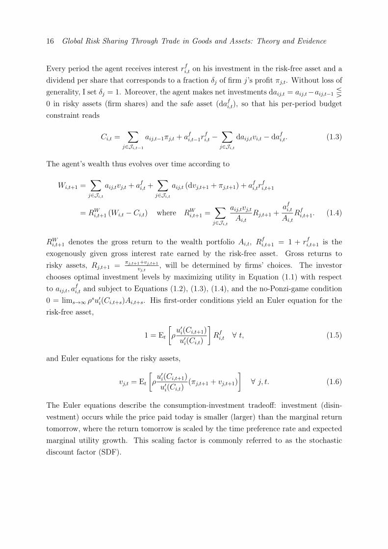
Every period the agent receives interest rfi,t on his investment in the risk-free asset and adividend per share that corresponds to a fraction δj of firm j’s profit πj,t. Without loss ofgenerality, I set δj = 1. Moreover, the agent makes net investments daij,t = aij,t−aij,t−1 Q
0 in risky assets (firm shares) and the safe asset (dafi,t), so that his per-period budgetconstraint reads
Ci,t =∑
j∈Ji,t−1
aij,t−1πj,t + afi,t−1rfi,t −
∑j∈Ji,t
daij,tvi,t − dafi,t. (1.3)
The agent’s wealth thus evolves over time according to
Wi,t+1 =∑j∈Ji,t
aij,tvj,t + afi,t +∑j∈Ji,t
aij,t (dvj,t+1 + πj,t+1) + afi,trfi,t+1
= RWi,t+1 (Wi,t − Ci,t) where RW
i,t+1 =∑j∈Ji,t
aij,tvj,tAi,t
Rj,t+1 +afi,tAi,t
Rfi,t+1. (1.4)
RWi,t+1 denotes the gross return to the wealth portfolio Ai,t, Rf
i,t+1 = 1 + rfi,t+1 is theexogenously given gross interest rate earned by the risk-free asset. Gross returns torisky assets, Rj,t+1 =
πj,t+1+vj,t+1
vj,t, will be determined by firms’ choices. The investor
chooses optimal investment levels by maximizing utility in Equation (1.1) with respectto aij,t, afi,t and subject to Equations (1.2), (1.3), (1.4), and the no-Ponzi-game condition0 = lims→∞ ρ
su′i(Ci,t+s)Ai,t+s. His first-order conditions yield an Euler equation for therisk-free asset,
1 = Et[ρu′i(Ci,t+1)
u′i(Ci,t)
]Rfi,t ∀ t, (1.5)
and Euler equations for the risky assets,
vj,t = Et[ρu′i(Ci,t+1)
u′i(Ci,t)(πj,t+1 + vj,t+1)
]∀ j, t. (1.6)
The Euler equations describe the consumption-investment tradeoff: investment (disin-vestment) occurs while the price paid today is smaller (larger) than the marginal returntomorrow, where the return tomorrow is scaled by the time preference rate and expectedmarginal utility growth. This scaling factor is commonly referred to as the stochasticdiscount factor (SDF).

Chapter 1 17
The Euler equations also describe the tradeoff between investing in different types ofassets. Chaining together Equation (1.6) and using Equation (1.5) yields
vj,t = Et∞∑s=1
ρsu′i(Ci,t+s)
u′i(Ci,t)πj,t+s =
∞∑s=1
Et [πj,t+s]
Rfi,t+s
+∞∑s=1
Covt[ρsu′i(Ci,t+s)
u′i(Ci,t), πj,t+s
]. (1.7)
The right-hand side of Equation (1.7) shows that an investor’s willingness to pay for ashare of firm j, which promises a risky dividend stream [πi,t+s]
∞s=1, is determined not only
by the expected value (discounted with the risk-free interest rate), but also by the payoff’scorrelation with
mi,t+s := ρsu′i(Ci,t+s)
u′i(Ci,t), (1.8)
the investor’s SDF. The SDF is an inverse measure of the investor’s well-being: in goodtimes, when expected consumption growth is high, the SDF is small since an additionalunit of expected consumption tomorrow is less valuable. In contrast, the SDF is large inbad times, when expected consumption is small and marginal utility is high. Equation(1.6) states that stocks that pay high dividends in times when expected marginal utility ishigh are more valuable to an investor.10 The investor buys risky assets (daij,t > 0) whilehis willingness to pay exceeds the price vj,t. He thus increases expected consumptiontomorrow at the expense of consumption today so that expected growth in marginalutility falls. Equation (1.5) thus commands that he partly disinvest the risk-free asset.Moreover, as the share of asset j in the investor’s total portfolio, aij,tvj,t
Ai,t, increases, asset
j becomes more correlated with the return on total wealth and thus less attractive as ameans of consumption smoothing. Hence, the investor’s willingness to pay for additionalunits of this asset decreases. The Euler equations thus relate investors’ willingness to payfor an asset to the asset’s price in equilibrium.
The assumption of a representative investor is innocuous in an economy where indi-viduals have identical beliefs about the probabilities with which uncertain events occur,the financial market is complete, and individuals’ preferences are of the von Neumann-Morgenstern type as described in Equation (1.1) (see Constantinides, 1982). Complete-ness of financial markets means that trading and creating state contingent assets is un-restricted and costless and hence idiosyncratic risks are insurable. Constantinides (1982)shows that under those conditions, equilibrium outcomes in an economy characterized by
10Note that this is an immediate implication of investors’ risk aversion. With risk neutrality (u′′ = 0),the discount factor would be constant and thus perfectly uncorrelated with any dividend stream.

18 Global Risk Sharing Through Trade in Goods and Assets: Theory and Evidence
optimal choices of investors exhibiting heterogeneous per-period utility functions and het-erogeneous levels of wealth are identical to the case where a “composite” investor owningthe sum of all inviduals’ wealth makes optimal decisions. Moreover, he shows that thecomposite investor’s preferences inherit the von Neumann-Morgenstern property and theconcavity of individuals’ utility functions.
The above setup of the financial market then encompasses three cases of financialmarket integration. Let Ii ⊆ I with i = 1, ..., ι denote mutually exclusive and collectivelyexhaustive sets of countries among which asset trade is unrestricted. Then ι = I denotesthe case where all countries are in financial autarky, so that there is one representativeinvestor for every single country in I and the set of available assets Ji,t is restricted to theset of domestic firms. The case of I > ι > 1 describes partially integrated internationalasset markets, where investor i is representative for every country in Ii and Ji,t comprisesthe firms from all countries in Ii. Finally, ι = 1 denotes the case of a fully integratedinternational financial market, where investor i is representative for all countries and hasunrestricted access to shares of all firms.
Note that the creation and trade of other “financial” assets within a complete market,that is, creation and trade of assets like derivatives, options, or futures, which are inzero net supply, has no bearing on the representative investor’s optimal consumption orinvestment decisions.11 This does not mean that none of those assets are traded; in fact,they are essential for eliminating idiosyncratic risk in the first place and facilitating adescription of the equilibrium by means of a representative investor. However, since bydefinition they must be in zero net supply, they cannot play a role in mitigating aggregaterisk and thus their presence does not have any impact on the tradeoff between risky assetsand the risk-free investment, nor do they have any bearing on the consumption-investmenttradeoff.
The Euler equations describe the demand side of the asset market. The risk-free assetis assumed to be in unlimited supply with an exogenous return Rf
i,t. In contrast, thesupply of primary assets and their stochastic properties will be endogenously determinedby firms’ entry and production decisions, which are described in the following section.
11I follow Dybvig and Ingersoll (1982)’s terminology in differentiating “financial” or “derivative” assetsfrom “primary” assets, where the former are defined by being in zero net supply and therefore, incontrast to the latter which are in positive net supply, have no impact on aggregate wealth of theeconomy. Firm shares are the prototype of primary assets. More generally, primary assets can becharacterized by the set of assets which form the aggregate asset wealth portfolio.
Chapter 1 19
1.3.2 Firm Behavior
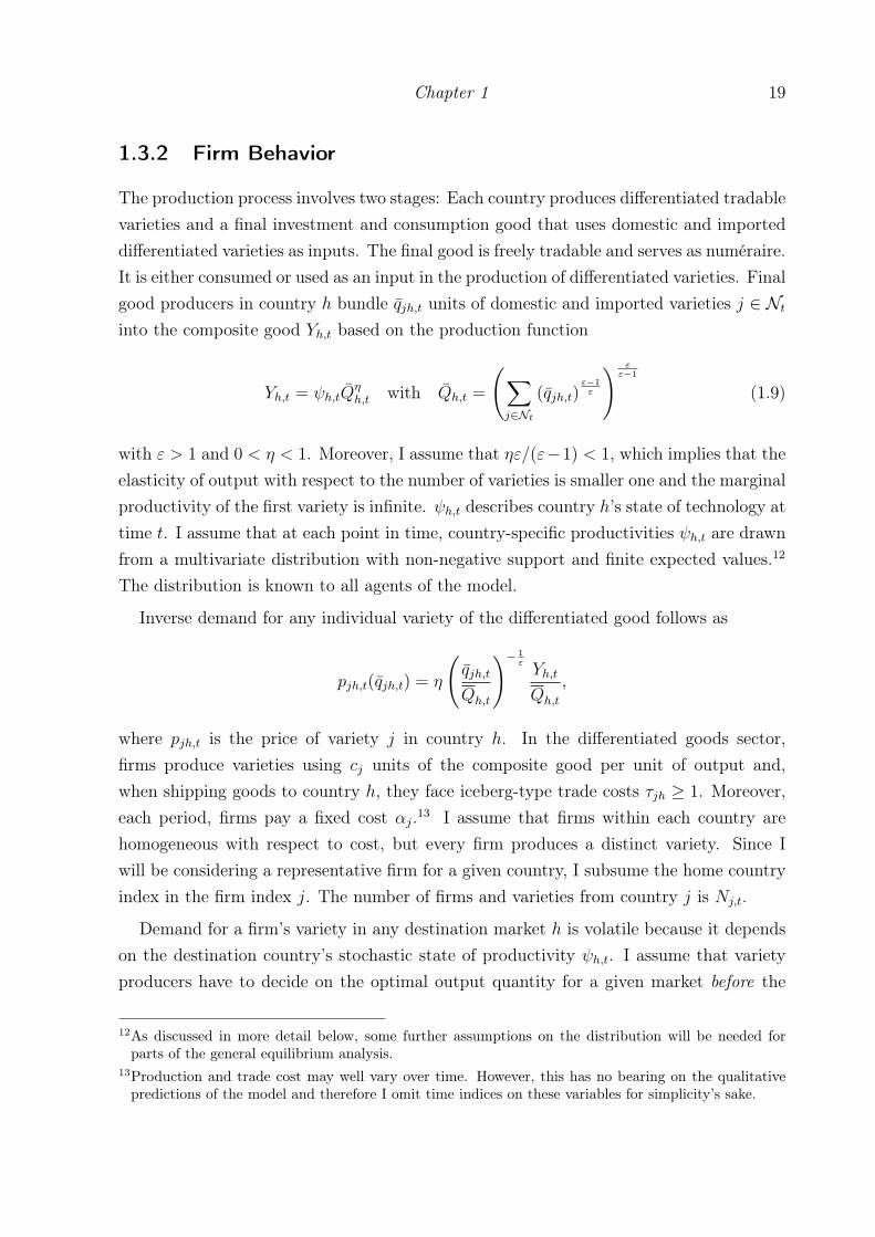
The production process involves two stages: Each country produces differentiated tradablevarieties and a final investment and consumption good that uses domestic and importeddifferentiated varieties as inputs. The final good is freely tradable and serves as numéraire.It is either consumed or used as an input in the production of differentiated varieties. Finalgood producers in country h bundle qjh,t units of domestic and imported varieties j ∈ Ntinto the composite good Yh,t based on the production function
Yh,t = ψh,tQηh,t with Qh,t =
(∑j∈Nt
(qjh,t)ε−1ε
) εε−1
(1.9)
with ε > 1 and 0 < η < 1. Moreover, I assume that ηε/(ε−1) < 1, which implies that theelasticity of output with respect to the number of varieties is smaller one and the marginalproductivity of the first variety is infinite. ψh,t describes country h’s state of technology attime t. I assume that at each point in time, country-specific productivities ψh,t are drawnfrom a multivariate distribution with non-negative support and finite expected values.12
The distribution is known to all agents of the model.
Inverse demand for any individual variety of the differentiated good follows as
pjh,t(qjh,t) = η
(qjh,t
Qh,t
)− 1εYh,t
Qh,t
,
where pjh,t is the price of variety j in country h. In the differentiated goods sector,firms produce varieties using cj units of the composite good per unit of output and,when shipping goods to country h, they face iceberg-type trade costs τjh ≥ 1. Moreover,each period, firms pay a fixed cost αj.13 I assume that firms within each country arehomogeneous with respect to cost, but every firm produces a distinct variety. Since Iwill be considering a representative firm for a given country, I subsume the home countryindex in the firm index j. The number of firms and varieties from country j is Nj,t.
Demand for a firm’s variety in any destination market h is volatile because it dependson the destination country’s stochastic state of productivity ψh,t. I assume that varietyproducers have to decide on the optimal output quantity for a given market before the
12As discussed in more detail below, some further assumptions on the distribution will be needed forparts of the general equilibrium analysis.
13Production and trade cost may well vary over time. However, this has no bearing on the qualitativepredictions of the model and therefore I omit time indices on these variables for simplicity’s sake.

20 Global Risk Sharing Through Trade in Goods and Assets: Theory and Evidence
productivity of the destination country is known because production and shipping taketime. Hence, at time t they choose the quantity qjh,t = qjh,t+1 to be sold in t + 1 andthey base this decision on the expected level of demand.14 Consequently, the amountof the composite good at time t is also determined a period in advance and follows as
Qh,t+1 = Qh,t =(∑
j∈I Nj,t (qjh,t)ε−1ε
) εε−1
.
With quantities determined, the price that variety producers expect depends on therealization of the stochastic productivity level in the destination country:
Et [pjh,t+1] = η
(qjh,tQh,t
)− 1ε
Qη−1h,t Et [ψh,t+1] = η
(qjh,tQh,t
)− 1ε Et [Yh,t+1]
Qh,t
(1.10)
At time t, firm j thus expects to make the following operating profit in market h at timet+ 1:
Et [πjh,t+1] = Et [pjh,t+1(qjh,t) · qjh,t − cjτjhqjh,t+1] (1.11)
Note that current revenue depends on the quantity produced at time t, while current costdepend on the quantity produced in t+ 1. Total profits are πj,t+1 =
∑h∈I πjh,t+1 − αj.
Firm j maximizes its net present value, acknowledging that its investors’ discount factoris stochastic and potentially correlated with the profit it expects to make in differentmarkets. As discussed above, firm j may obtain financing from investors in multiplecountries, depending on the degree of financial market integration. Lets assume, withoutloss of generality, that the firm’s home country j is part of the set of countries Ii whoseasset markets are fully integrated. Then, the relevant discount factor for firm j is mj
t+s =
mi,t+s. The firm takes the distribution of the SDF as given; hence, its optimizationproblem reads
max[qjh,t+s≥0]∞s=0 ∀h
Vj,t = Et
[∞∑s=0
mjt+s · πj,t+s
].
14I have thus implicitly assumed that firms cannot reallocate quantities across markets once the uncer-tainty about demand has been resolved, and that they do not hold inventory in destination countries.

Chapter 1 21
Since quantities can always be adjusted one period ahead of sales, the optimal choice ofqjh,t at any time t can be simplified to a two-period problem, that is,
maxqjh,t≥0 ∀h
Et
[mjt+1 ·
∑h∈I
pjh,t+1(qjh,t) · qjh,t
]−∑h∈I
cjτjhqjh,t − αj
=∑h∈I
η
(qjh,tQh,t
) ε−1ε (
Et [Yh,t+1]Et[mjt+1
]+ Covt
[mjt+1, Yh,t+1
])−∑h∈I
cjτjhqjh,t − αj.
The first-order condition yields an optimal quantity for any market h that is produced attime t and to be sold in t+ 1 equal to
q∗jh,t =θ(1 + λjh,t)
ε(Rfj,t+1cjτjh
)−ε∑
j∈I Nj,t(1 + λjh,t)ε−1(Rfj,t+1cjτjh
)1−ε · Et [Yh,t+1] , (1.12)
where I have defined θ := η(ε−1)ε
< 1 and
λjh,t := Rfj,t+1Covt
[mjt+1,
Yh,t+1
Et [Yh,t+1]
].
To arrive at Equation (1.12), I used Qε−1ε
h,t =∑
j∈I Nj,t(q∗jh,t)
ε−1ε and Equation (1.5) to
substitute for the expected value of the SDF. I call λjh,t the “risk premium” of market h.It is negative for markets that are risky in the sense that demand shocks on these marketsare negatively correlated with the SDF, and positive otherwise. Equation (1.9) impliesthat demand growth comoves one to one with the country-specific productivity shocksEt [ψh,t+1] /ψh,t+1.
Equation (1.12) states that firms ship larger quantities to markets with lower tradecost and higher expected demand. They ship less in times of high real interest rates,that is, when current consumption is highly valued over consumption tomorrow, becauseproduction cost and trade cost accrue in t, while revenue is obtained in t+ 1. Moreover,firms ship more to those markets where demand growth is positively correlated with theirinvestors’ SDF, since investors value revenues more if, ceteris paribus, they tend to be highin bad times and low in good times. This is the central prediction of the model, which Ibelieve is new to the trade literature, and will be subjected to empirical testing in Section1.4. First, however, I relate the model’s predictions to the standard gravity frameworkand close the model to show how the risk premia are determined in general equilibriumand how they can be estimated. I also show that they will be zero only under specialcircumstances, namely, if the exogenous distribution of productivity shocks and financial

22 Global Risk Sharing Through Trade in Goods and Assets: Theory and Evidence
market integration permit complete elimination of aggregate risk, and if investors, tradingoff risk against returns, endogenously choose to do so.
Once the state of the destination country’s productivity is revealed in t+ 1, the firm’srevenue in market h obtains as
pjh,t+1(q∗jh,t)q∗jh,t = φjh,tYh,t+1, (1.13)
where
φjh,t =
(q∗jh,tQjh,t
) ε−1ε
=(1 + λjh,t)
ε−1(Rfj,t+1cjτjh
)1−ε
∑j∈I Nj,t(1 + λjh,t)
ε−1(Rfj,t+1cjτjh
)1−ε
denotes firm j’s trade share in market h, that is, the share of country h’s real expendituredevoted to firm j. Equation (1.13) is a firm-level gravity equation with bilateral tradecost augmented by a risk-adjusted interest rate. Note that Equation (1.13) nests thegravity equation of derived from the model of Krugman (1980) with homogenous firmsand monopolistic competion as a special case.15 In fact, there are a number of special casesunder which sales predicted by the model follow the standard law of gravity. Suppose, first,that the time lag between production and sales is eliminated. Then, demand volatilitybecomes irrelevant as firms can always optimally adjust quantities to the current demandlevel (Et [Yh,t] = Yh,t). Next, suppose that investors are risk neutral, so that marginalutility is constant. Then, the SDF does not vary over time and hence has a zero covariancewith demand shocks. In this case, Equation (1.13) will differ from the standard gravityequation only due to the presence of the time lag, which introduces the risk-free rateas an additional cost parameter. The same relationship obtains if demand growth isdeterministic. Moreover, full integration of international financial markets will equalizeSDFs across countries, so that the covariance terms (and the risk-free rates) are identicalacross source countries and hence cancel each other out in the trade share equation. Note,however, that in this last case, the covariance will still influence optimal quantities asdescribed in Equation (1.12). Firms still ship larger quantities to countries with positiveλs and investors value these firms more, but since all their competitors from other countriesbehave accordingly, trade shares are independent of λ. Finally, covariances could be setto zero endogenously, a possible but unlikely case, as I will discuss in more detail below.
15See, for example, Head and Mayer (2014) for a description of this model.

Chapter 1 23
Firm j’s maximum net present value is given by
V ∗j,t =∑h∈I
(Et[mjt+1 · pjh,t+1(q∗jh,t)q
∗jh,t
]− cjτjhq∗jh,t
)− αj (1.14)
=∑h∈I
(1− θ)1 + λjh,t
Rfj,t+1
φjh,tEt [Yh,t+1]− αj,
the sum of expected sales, adjusted by an inverse markup factor 0 < (1 − θ) < 1 anddiscounted with a market-specific risk-adjusted interest rate, minus fixed cost.
1.3.3 Model Closure
1.3.3.1 Firm Entry and Asset Market Clearing
Firm entry governs the supply of assets from every country. I assume that there are nobarriers to entry; hence, firms enter as long as their net present value is non-negative. Inview of Equation (1.14), this implies that in equilibrium
V ∗j,t = 0 ⇔ Et
[mjt+1 ·
∑h∈I
pjh,t+1(q∗jh,t)q∗jh,t
]=∑h∈I
cjτjhq∗jh,t + αj. (1.15)
Entry lowers the price of incumbents’ varieties and thus their profits due to the concavity ofthe final goods production function in the composite good.16 Moreover, entry of additionalfirms from country j implies that the share of assets of this particular type in the investor’sportfolio increases and the asset becomes more risky in the sense that its payoff correlatesmore with the investor’s total wealth. Hence, V ∗j,t is driven down to zero as new firmsenter. Equation (1.15) determines the number of firms and thus the supply of assets fromevery country. Asset market clearing implies
Nj,t = aij,t ∀ j ∈ Ii, (1.16)
that is, the number of variety producers in country j is equal to the representative investori’s demand for shares of this particular type.17 Remember that depending on the degree
16There is a countervailing positive effect of firm entry on incumbents’ profits arising from the love ofvariety inherent to the CES production function of the composite good, which is inversely related toε, the elasticity of substitution. The assumption that ηε/(ε− 1) < 1 assures that concavity dominateslove for variety.
17Remember that I have normalized the number of shares per firm to unity.

24 Global Risk Sharing Through Trade in Goods and Assets: Theory and Evidence
of financial market integration, the representative investor’s demand equals the compositedemand of all individuals from country j or from (a subset of) all countries.
Combining the entry condition (1.15) with the Euler equation (1.6) that governs assetdemand and substituting
∑h∈I pjh,t+1(q∗jh,t) · q∗jh,t = πj,t+1 +
∑h∈I cjτjhq
∗jh,t+1 +αj implies
that the equilibrium asset price equals the cost of setting up a new firm, that is,
vj,t =∑h∈I
cjτjhq∗jh,t + αj. (1.17)
With asset prices and profits determined, the returns to holding firm shares can bedescribed in terms of country-specific demand growth, which, by Equation (1.9), correlatesperfectly with the productivity shocks. Using Equations (1.13), I obtain
Rj,t+1 =πj,t+1 + vj,t+1
vj,t=∑h∈I
φjh,tEt [Yh,t+1]
vj,t
(Yh,t+1
Et [Yh,t+1]
)(1.18)
as the gross return of a share of firm j. Returns are linear combinations of demand growthin the destination markets, where markets are weighted by the share of expected sales inthe total discounted value of the firm.
1.3.3.2 Equilibrium
Let N t, ψt+1, qj,t denote (I × 1) vectors collecting, respectively, the number of firms,the productivity levels, and firm j’s optimal quantity in each country h = 1, ..., I. Thenqt =
[q′1,t, ..., q
′i,t, ..., q
′I,t
]is a (I×I) matrix of all firms’ sales across all markets. Moreover,
let ai,t denote the (Ii × 1) vector of investor i’s optimally chosen number of shares ofall representative firms j ∈ Ii, where Ii is the number of countries in Ii. πit+1 and vitdenote (Ii × 1) vectors of these firms’ profits and share prices, respectively. I use a tildeto indicate random variables defined by a conditional density function. For example,ψt+1 describes the joint distribution of the productivity levels f(ψt+1|Ψt) conditionalon the history of realized productivity shocks. Then, the set of equilibrium conditionsdetermining the endogenous variables qt, N t, {ai,t}ιi=1, {a
fi,t}ιi=1, {vit}ιi=1, {Ci,t}ιi=1, and,
for all s = 1, ...,∞, qt+s, N t+s, {πit+s}ιi=1, {vit+s}ιi=1, {mi,t+s}ιi=1, {Ci,t+s}ιi=1 is given by
Investors’ first-order conditions (1.5) and (1.6):
afi,t
[mi,t+1;Rf
i,t+1
]and aij,t [vj,t, πj,t+1, mi,t+1] ∀ j ∈ Ii and i = 1, ..., ι

Chapter 1 25
Firms’ first-order conditions (1.12): qj,t[qt,N t, mi,t+1; ψt+1
]∀ j ∈ Ii and i = 1, ..., ι
Profits (1.11): πj,t+1
[qt,N t; ψt+1
]∀ j ∈ Ii and i = 1, ..., ι
Free entry condition (1.15): Nj,t
[qt,N t, mi,t+1; ψt+1
]∀ j ∈ Ii and i = 1, ..., ι
Asset market clearing (1.16): aij,t [Nj,t] ∀ j ∈ Ii and i = 1, ..., ι
Stochastic discount factor (1.8): mi,t+1
[Ci,t, Ci,t+1
]∀ i = 1, ..., ι
Budget constraint (1.3): Ci,t
[afi,t,ai,t,v
it;Wi,t
]and
Ci,t+1
[afi,t,ai,t, π
it+1, a
fi,t+1, ai,t+1, v
it+1;Rf
i,t+1
]∀ i = 1, ..., ι
and the no-Ponzi-game condition 0 = lims→∞mi,t+sAi,t+s ∀ i = 1, ..., ι.18
This describes the equilibrium from the point of view of the representative investors forthe ι subsets of countries. If financial markets are partially or fully integrated (ι > 1), theequilibrium values for investment and consumption describe aggregates of all countries inIi. Hence, consumption or investment on the national level, as well as bilateral financialflows, are not determined at this point. To pin down those values in the case of (par-tially) integrated international financial markets, further assumptions on the distributionof wealth and the utility functions are needed. Note that up to this point and also inwhat follows, no restrictions are placed on the distribution of wealth across countries oreven across individuals. The only assumptions about preferences made so far state thatall individuals’ utility functions are of the von Neumann-Morgenstern-type and exhibitrisk aversion. In Appendix A1.2, I show how countries’ current accounts can be derivedonce country-level consumption and bilateral investment flows are determined.19
18I include a subset of the exogenous or predetermined variables, separated by a semicolon, whereeverthis seems conducive to conveying the intuition behind the conditions. Also, remember that I usesuperscript j on the variables m, Rf , and λ to denote the SDF, the risk-free rate, and the risk premiarelevant to firm j and subscript i to denote the SDF, the risk-free rate, and the risk premia of investorsfrom country i. For all j ∈ Ii,mj
t+1 = mi,t+1, λjh,t = λih,t ∀ h ∈ I, and Rfj,t+1 = Rfi,t+1.
19Country-level (or even individual-level) consumption and bilateral investment flows can, for example,easily be determined under the assumption that individuals’ preference exhibit identical degrees ofconstant relative risk aversion, that is, all individuals per-period utility functions observe u(ci,t) =
c(1−γ)i,t /(1−γ) for γ > 1 or u(ci,t) = ln ci,t. Then, every individual in an integrated financial market willown a fraction of the same wealth portfolio, which is the portfolio chosen by the representative agent.The fraction owned by an individual corresponds to his share of wealth in total wealth. Analogously,individual consumption is proportional to consumption of the representative investor, depending, again,only on the individual’s share in total wealth (see Rubinstein, 1974 and Grossman and Razin, 1984).

26 Global Risk Sharing Through Trade in Goods and Assets: Theory and Evidence
1.3.3.3 The Stochastic Discount Factor and Country Risk Premia
This section shows how the distribution of the SDF derives from the distribution ofcountry-specific productivity shocks in order to understand how the country risk premiaλih,t = Rf
i,t+1Covt[mi,t+1,
˜Y h,t+1
]are determined and how they develop over time. Opti-
mal consumption and investment plans in conjunction with the stochastic properties offirms’ profits pin down the distribution of future consumption and link the SDF to thecountry-specific shocks. To make this link explicit, I impose an additional assumption onthe stochastic nature of the productivity levels. Specifically, I assume that the produc-tivity levels are indepently and identically distributed over time and follow a multivariatelognormal distribution. This assumption facilitates describing the SDF in terms of cur-rent consumption and next-period wealth, with the latter being directly affected by thecountry-specific productivity shocks through the profits of firms in the investor’s portfolio.
Using the budget constraint (1.3) together with Equations (1.2) and (1.4), equilibriumconsumption of the representative investor i can be expressed in terms of asset wealth andthe return to the wealth portfolio. Substituting optimal consumption plans for Ci,t andCi,t+1 in mi,t+1 yields mi,t+1 = fi(Ai,t−1, R
Wi,t , Ai,t, R
Wi,t+1, Ai,t+1). Moreover, Ai,t+1 can be
replaced by the sequence of optimal future investments, which depend on initial wealthand the evolution of asset prices and returns, to pin down the SDF as
mi,t+1 = fi
(Ai,t−1, R
Wi,t , Ai,t, R
Wi,t+1, {v
it+s}∞s=1, {π
it+s}∞s=1, {R
fi,t+s}∞s=1
), (1.19)
a function of current wealth and investment and exogenous parameters (from the investor’spoint of view) only. See Appendix A1.1 for details of the derivation.
Generally, the precise relationship fi(·) depends crucially on two fundamentals; thenature of the stochastic processes guiding the distribution of returns and the functionalform of ui(·).20 Fama (1970) showed that the multiperiod consumption choice problemcan be reduced to a two-period problem of choosing between today’s consumption and
It follows that for all countries k, j in Ii, country-level consumption Ck,t and bilateral investment akj,tare proportional to the representative investor i’s consumption Ci and investment into the firms fromall countries in Ii, aij,t, with the factor of proportionality equal toWk,t/Wi,t whereWi,t =
∑k∈IiWk,t.
20If the shocks are independent over time, fluctuations in returns do not indicate changes in investmentopportunities and do no affect total discounted future wealth of the infinitely lived agent. In contrast, ifreturns are non-stationary, changes in returns do imply changes in investors’ total wealth and changesin the set of investment opportunities and, therefore, may affect long-run consumption plans. Howquickly investors return to the their steady long-run consumption level after a temporary shock cru-cially depends on the elasticity of intertemporal substitution, a feature inherent to u(·). If shocks arepermanent, u(·) determines whether income effects of higher expected returns in the future on currentconsumption dominate substitution effects from changes in the incentive to invest.

Chapter 1 27
tomorrow’s wealth if investment returns are independently and identically distributed overtime, that is, if the set of investment opportunities is independent of the current state orpast states of the economy. This implies, that fi(·) can be written as gi,t(RW
i,t+1), a functionof the return to wealth in t+ 1 and variables determined in the previous period, with thelatter being subsumed in the i, t index of the function. Moreover, as the pioneers of theCapital Asset Pricing Model (CAPM) (Sharpe, 1964; Lintner, n.d.; and Black, 1972) haveshown, gi,t(·) is linear in RW
i,t+1 if returns are normally distributed, independently of thefunctional form of ui(·).
Let us assume that productivity levels are lognormally distributed with constant meanand variance, that is, ∀ t
ψt ∼ Lognormal (µ,Σ) . (1.20)
Then, productivity shocks follow an approximate normal distribution ˜ψt ∼apprx.
N(µψ,Σψ
),
where ˜ψt =
[˜ψ1,t, ...,
˜ψh,t, ...,
˜ψI,t
]′with typical element ˜ψh,t =
ψh,t−Et−1[ψh,t]Et−1[ψh,t]
. The approx-
imation works best in the neighborhood of zero. Rewriting returns in Equation (1.18)using Equation (1.9) as
Rj,t+1 =∑h∈I
φjh,tQηh,tµh
vj,t· ˜ψh,t+1
shows that returns are linear combinations of productivity shocks. Hence, they inheritthe approximate normal distribution. Moreover, from the investor’s point of view attime t, future returns follow i.i.d. distributions as well if he does not expect changes inφjh, Qh(q,N ), and vj in any future period t+s to be systematically related to realizationsof ψ.21 Under those assumptions, the results of Fama (1970) can be applied to obtain alinear discount factor model:
mi,t+1 = ζi,t + γi,tRWi,t+1 where γi,t < 0. (1.21)
For details of the derivation, which in parts follows Cochrane (2005), Chapter 9, seeAppendix A1.1.
21This requires a certain degree of myopia on the part of investors. Specifically, it requires assuming thatinvestors do not take into account general equilibrium adjustments in the number of firms and theirmarket-specific profits following a specific realization of global productivity levels at any future date.

28 Global Risk Sharing Through Trade in Goods and Assets: Theory and Evidence
The linear model for the SDF facilitates deriving an explicit expression for λ′i,t =
[λi1,t, ..., λih,t, ..., λiI,t], the covariances of the SDF with the country-specific productivityshocks. To ease notation, I henceforth drop the tilde symbol for random variables. UsingEquation (1.18) together with the expression for RW
i,t+1 in Equation (1.4), the SDF can bewritten as a linear function of asset returns:
mi,t+1 = ζi,t + γi,t∑j∈Ji,t
aij,tAi,t
∑h
φjh,tEt [Yh,t+1]
(Yh,t+1
Et [Yh,t+1]
)(1.22)
Equation (1.22) implies that partial covariances of mi,t+1 with demand growth in anycountry h are given by the coefficients from a linear regression of the form mi,t+1 =
bi0,t + b′i,tYt+1 with b′i,t = [bi1,t, ..., bih,t, ..., biH,t] and Y′t =
[Y1,t, ..., Yh,t, ..., YI,t
], where
bih,t = γi,t∑j∈Ji,t
aij,tAi,t
φjh,tEt [Yh,t+1] . (1.23)
Equation (1.23) shows that the partial correlation of the SDF with country h’s demandgrowth is a weighted sum of exports by all firms in the investor’s portfolio, where each firmis weighted by its portfolio share. Note that the theory implies γi,t < 0; hence, a largerexposure to demand growth in h through higher exports implies a stronger negative partialcorrelation with the SDF. What matters for investors’ perception of riskiness, however,is not the partial correlation, but the overall correlation, which takes into account thatfirms also sell to other countries exhibiting demand shocks that may be correlated withthe shocks in country h. The covariances of country-specific shocks with country i’s SDF(scaled with the risk-free rate) are thus given by
λi,t = Rfi,t+1Covt
[mi,t+1, Y t+1
]= Rf
i,t+1Covt[Y t+1, Y
′t+1
]bi,t, (1.24)
with hth element equal to
λih,t = Rfi,t+1Covt
[mi,t+1, Yh,t+1
]= Rf
i,t+1
(σYht
)2
bih,t +Rfi,t+1
∑k 6=h
σYh,Ykt bik,t. (1.25)
Note that the bs are themselves functions of the λs so that Equation (1.25) is an implicitexpression for λih,t.
Using the linear SDF from Equation (1.22) to rewrite the Euler equation (1.6) as
Et [Rj,t+1]−Rfi,t+1 = −λ′i,tβj,t (1.26)

Chapter 1 29
shows that the λs can be interpreted as monetary risk premia.22 Equation (1.26) decom-poses the return that j’s share earns in excess of the risk-free rate on average, which is thecompensation investors demand for its riskiness, into a risk price and a risk quantity asso-ciated with the firm’s activity in every market. The quantity component, βjh,t, measuresfirm j’s exposure to demand volatility in market h. More precisely, βjh,t is the elasticityof the firm’s value with respect to demand growth in market h. According to Equation(1.18), it equals the share of expected sales in market h in the total present value of the
firm, that is, βjh,t =φjh,tEt[Yh,t+1]
vj,t. The λs measure how much compensation in terms of
average return in excess of the risk-free rate investors demand per unit of exposure βjh,tto volatility in market h.
1.3.4 Equilibrium Risk Premia and the Risk-Return Tradeoff
The risk premia obtaining in equilibrium are outcomes of investors’ risk-return tradeoff.This section explains the intuition behind this tradeoff and, more specifically, it showsthat the risk premia will generally be nonzero, even with perfectly integrated interna-tional asset markets. In complete financial markets investors can freely trade and createassets. However, the creation of primary assets is subject to the stochastic properties ofthe investment opportunities, and the creation of other financial assets is subject to therestriction that they be in zero net supply in equilibrium. The latter implies that financialassets can be used to eliminate investors’ idiosyncratic risk, but have no role in mitigatingaggregate risk, since zero net supply means that somebody’s gain from holding such anasset must be somebody else’s loss.
The amount of aggregate risk present in equilibrium, defined as volatility of the SDF,is thus purely an outcome of investment choices. Aggregate risk is absent if and only ifconsumption does not vary over time. Equation (1.22) shows that the volatility of theSDF derives from the volatility of the country-specific shocks, where the individual coun-tries’ contributions depend on firms’ export choices φjh,tEt[Yh,t+1] and investors’ portfoliochoices aij,t. It is apparent that the potential for eliminating consumption risk throughportfolio management is constrained by the correlation pattern of country shocks. Unlesssome shocks are perfectly negatively correlated, the only way to set the variance of theSDF to zero is zero investment in risky assets. This means that no firm is active andinvestors put all their savings into the risk-free asset. All λs will then be zero. For this
22See Appendix A1.3 for details of the derivation.

30 Global Risk Sharing Through Trade in Goods and Assets: Theory and Evidence
to be an equilibrium outcome, however, the value of creating a new firm must be zero.Rewriting Equation (1.14) in terms of exogenous variables and λ only yields
V ∗j,t =1− θθ
ηη−1
∑h∈I
(1 + λjh,t
Rfj,t+1
)ε(cjτjh)
−εEt [ψh,t+1]η
1−η(∑j∈I Nj(cjτjhR
fj,t+1)1−ε(1 + λjh,t)
ε−1) ε−ηε−1
(ε−1)(η−1)
− αj.
(1.27)
Since ε − ηε − 1 < 0, the value of creating a new firm goes to infinity as the numberof firms approaches zero. This owes to the fact that marginal productivity of the firstvariety is infinite, by the assumption that ηε
ε−1< 1, and it holds for λ Q 0. Hence, avoiding
any exposure to aggregate risk by not investing into firms at all cannot be an equilibriumoutcome.
Now suppose that the covariance structure of country shocks permits hedging aggregaterisk because at least one country’s shocks are perfectly negatively correlated with therest. Investors can exploit the hedging opportunity by buying firms from the countrywith negatively correlated shocks. Or, more generally, by buying firms that sell a lotto this market. This is precisely what the Euler equation commands: the willingnessto pay is larger for assets that correlate positively with the SDF. However, only underspecial conditions will it be optimal to exploit the hedging opportunity to its full extent,that is, to completely eliminate aggregate risk. The reason lies again with the decreasingreturns to scale inherent in the production function. Financing more firms that ship alot to a certain destination market that correlates negatively with the SDF means thatthe amount of the composite good produced in this country increases. This implies adecrease in the marginal productivity of the composite good and a decrease in firms’expected market-specific profits. Equation (1.27) shows that, ceteris paribus, the value ofan individual firm falls in the number of firms selling to a given market. Hence, investorsare faced with a classical risk-return tradeoff where the optimal choice is generally not tofully eliminate aggregate risk.
A two-country example makes this point very clear. Suppose there are only two coun-tries i and h, which are identical with regard to production cost for varieties, trade cost,and the risk-free rate. That is, suppose I = (i, h), ci = ch = c, αi = αj = α, τih = τhi =
τ, τii = τhh = 1. Moreover, suppose that the variance of productivity shocks is identical inboth countries, σψh = σψi = σψ = σY , and that shocks are perfectly negatively correlated,ρYi,Yh = σYi,Yh
σYiσYh= −1. The two countries may differ in their initial level of asset wealth
Ai,t Q Ah,t and in the mean of the productivity level. Further suppose, without loss ofgenerality, that Et [ψh,t+1] ≥ Et [ψi,t+1]. Finally, assume, for simplicity, that asset mar-

Chapter 1 31
kets are fully integrated and preferences exhibit constant relative risk aversion. Completeelimination of aggregate risk would then imply that the country risk premia as describedin Equation (1.25) jointly obey
λk,` = Rfk,t+1Covt
[mk,t+1, Y`,t+1
]= 0 ∀ k, ` = i, h
⇔ Et [Y`,t+1] (ak`φ``,t + akkφk`,t) = −ρYk,Y` · Et [Yk,t+1] (akkφkk,t + ak`φ`k,t) ∀ k, ` = i, h
⇔ Et [Yh,t+1] = Et [Yi,t+1] . (1.28)
The third step follows from the fact that with fully integrated international asset marketsand constant and equal degrees of relative risk aversion, investors in both countries willown a share of the same international market portfolio. That is, aii,t = ϕNi,t, ahi,t =
(1 − ϕ)Ni,t, aih,t = ϕNh,t, ahh,t = (1 − ϕ)Nh,t, where ϕ/(1 − ϕ) = Ah,t/Ai,t. Equation(1.28) states that zero risk premia obtain if expected final goods production between thetwo countries is equalized. Note that Equation (1.28) together with Et [ψi,t+1] ≤ Et [ψh,t+1]
impliesQi,t ≥ Qh,t, that is, the output of the composite good is larger in the less productivemarket. This already suggests that an allocation yielding λih = 0 is not efficient. To makethis argument formally, I show in Appendix A1.4 that to obtain equal expected outputin both countries, the number of firms in the less productive country i must be largerand, hence, firms from country i face a more competitive environment. This is reflectedin smaller equilibrium net present values of firms from country i compared to firms fromcountry h, which is inconsistent with the free entry condition mandating that net presentvalues be equal and zero in both countries. It follows that λk` = 0 ∀ k, ` = i, h can be anequilibrium consistent with optimal choices of firms and investors only in the knife-edgecase where Et [ψh,t+1] = Et [ψi,t+1].
Generally, firms make larger profits by selling more to more productive and less crowdedmarkets. The amount of aggregate risk taken on by investors in equilibrium balances theincentive to finance firms that make higher profits with the desire for smooth consumption.Perfect consumption insurance and zero risk premia are feasible but suboptimal if investorsput all their wealth into the risk-free asset. Alternatively, perfect consumption insuranceand positive investment in firms is possible when, for every country, there is at leastone other country exhibiting perfectly negatively correlated shocks. But even then, zeroaggregate risk will be an equilibrium outcome only in special cases, such as the one justoutlined.
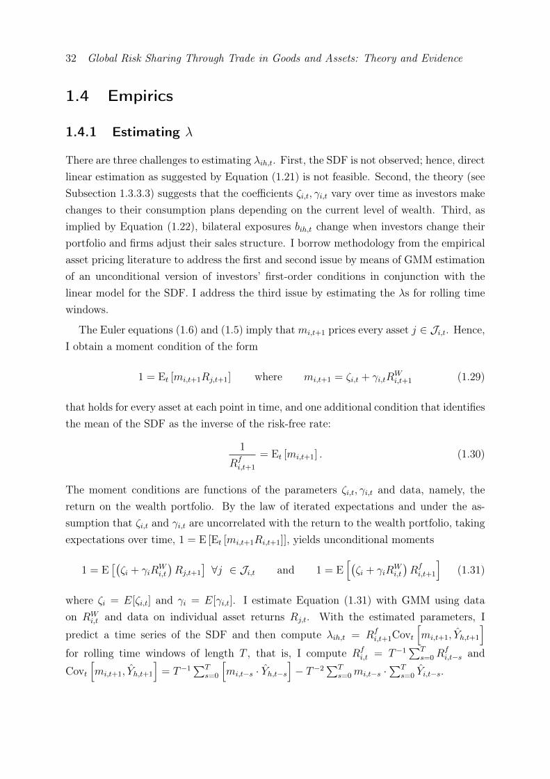
32 Global Risk Sharing Through Trade in Goods and Assets: Theory and Evidence
1.4 Empirics
1.4.1 Estimating λ
There are three challenges to estimating λih,t. First, the SDF is not observed; hence, directlinear estimation as suggested by Equation (1.21) is not feasible. Second, the theory (seeSubsection 1.3.3.3) suggests that the coefficients ζi,t, γi,t vary over time as investors makechanges to their consumption plans depending on the current level of wealth. Third, asimplied by Equation (1.22), bilateral exposures bih,t change when investors change theirportfolio and firms adjust their sales structure. I borrow methodology from the empiricalasset pricing literature to address the first and second issue by means of GMM estimationof an unconditional version of investors’ first-order conditions in conjunction with thelinear model for the SDF. I address the third issue by estimating the λs for rolling timewindows.
The Euler equations (1.6) and (1.5) imply thatmi,t+1 prices every asset j ∈ Ji,t. Hence,I obtain a moment condition of the form
1 = Et [mi,t+1Rj,t+1] where mi,t+1 = ζi,t + γi,tRWi,t+1 (1.29)
that holds for every asset at each point in time, and one additional condition that identifiesthe mean of the SDF as the inverse of the risk-free rate:
1
Rfi,t+1
= Et [mi,t+1] . (1.30)
The moment conditions are functions of the parameters ζi,t, γi,t and data, namely, thereturn on the wealth portfolio. By the law of iterated expectations and under the as-sumption that ζi,t and γi,t are uncorrelated with the return to the wealth portfolio, takingexpectations over time, 1 = E [Et [mi,t+1Ri,t+1]], yields unconditional moments
1 = E[(ζi + γiR
Wi,t
)Rj,t+1
]∀j ∈ Ji,t and 1 = E
[(ζi + γiR
Wi,t
)Rfi,t+1
](1.31)
where ζi = E[ζi,t] and γi = E[γi,t]. I estimate Equation (1.31) with GMM using dataon RW
i,t and data on individual asset returns Rj,t. With the estimated parameters, I
predict a time series of the SDF and then compute λih,t = Rfi,t+1Covt
[mi,t+1, Yh,t+1
]for rolling time windows of length T , that is, I compute Rf
i,t = T−1∑T
s=0Rfi,t−s and
Covt[mi,t+1, Yh,t+1
]= T−1
∑Ts=0
[mi,t−s · Yh,t−s
]− T−2
∑Ts=0 mi,t−s ·
∑Ts=0 Yi,t−s.

Chapter 1 33
Table 1.1: Summary statistic of return and import growth data
Return data #Obs. Mean Std. Dev. Min MaxTime 450 1977M1 2014M6rf 450 0.41 0.29 0 1.35rW 450 1.02 4.49 -22.64 12.89Re 49 .73 .17 .37 1.24
Import growth dataTime 360 1983M1 2012M12µY 180 0.04 0.05 0.01 0.45σY 180 0.27 0.35 0.06 2.61
Returns in %. Re is the average excess return (gross return minus risk-free rate)of industry portfolios over time. µY (σY ) denotes the mean (standard deviation)of country-specific demand shocks over time.
1.4.2 Estimating λs for the U.S. Financial Market
I estimate risk premia with respect to 175 countries for the U.S. financial market, since myempirical analysis of the impact of risk premia on exports will be based on U.S. exports.Hence, I assume that the SDF of investors trading on the U.S. financial market is therelevant SDF for U.S. firms. As discussed above, this is consistent with the cases whereinvestors from (a subset of) all countries (including the United States) trade freely on asupranational asset market as well as with financial autarky. The export data span theyears 1992 to 2012 and I estimate a λUSh,t for every market in every year based on datareaching back 10 years into the past. That is, I estimate the covariance of demand shocksand the mean of the risk-free rate based on the 10 most recent years.
1.4.2.1 Data
For monthly asset returns I use 49 value-weighted industry portfolios provided by KennethR. French through his Data Library.23 The portfolios are constructed based on all stockstraded on NYSE, AMEX, and NASDAQ. Theoretically, every asset and every portfolioof assets available to U.S. investors could be used to estimate Equation (1.31). FigureA1.2 in the Appendix plots the distribution of excess returns to the industry portfolios.A robustness check with regard to this choice of test assets will be provided. I follow theasset pricing literature by approximating RW
t , the return on the wealth portfolio, with
23http://mba.tuck.dartmouth.edu/pages/faculty/ken.french/data_library.html

34 Global Risk Sharing Through Trade in Goods and Assets: Theory and Evidence
Table 1.2: Parameter estimates of the linear SDF model
Time period: 1977M1–2014M6 1977M1– 1989M6 1989M7–2001M12 2002M1–2014M6ζUS 1 .99 1 1
[t-stat.] [133] [90.4] [80.2] [80.2]γUS -3.37 -2.92 -3.81 -3.61
[t-stat.] [-2.54] [-1.50] [-1.86] [-1.24]# Moment Conditions 50 50 50 50
# Observations 450 150 150 150# Parameters 2 2 2 2
Test of joint signific.: χ2e 49280 35166 12818 17206
P(χ22 > χ2
e) 0 0 0 0J-Test: J-Stat 97 397.8 161.5 196.8P(χ2
48 > J) 0 0 0 0
Results from first-stage GMM.
the return to the value-weighted market portfolio including all stocks traded on NYSE,AMEX, and NASDAQ. Monthly data on the market portfolio and the risk-free rate arealso from Kenneth R. French’s Data Library.
I use total monthly imports by country obtained from the IMF’s Direction of TradeDatabase to measure demand growth. Growth is measured with respect to the previousmonth and rates are adjusted for constant monthly factors. Table 1.1 summarizes thedata used to estimate the risk premia. The data appendix A1.5 gives details more details.
1.4.2.2 Results
Table 1.2 summarizes the results from GMM estimation of Equation (1.31). Column (1)shows parameter estimates based on the full sample period, which are strongly signifi-cant. As suggested by the theory, γ is negative; hence, the return to market portfolio isnegatively related to the SDF. Columns (2) through (4) repeat the estimation for consec-utive subperiods of the sample, each covering 12.5 years. In view of the assumption thatthe coefficients ζi,t, γi,t are uncorrelated with returns, which underlies the unconditionalmoments (1.31), it is reassuring that the estimates barely change over time.
I use the estimates in Column (1) to predict a time series of the SDF in accordancewith Equation (1.21) and then compute covariances with import growth scaled with theaverage risk-free rate as in Equation (1.25) for each point in time, always going back 120months into the past. Figure 1.1 presents an overview of the results. The left panel plotscorrelation coefficients based on 10-year windows of monthly import growth data and thepredicted time series of the SDF; the right panel shows the distribution of estimated λs.Both panels show that the median values, as well as the whole distribution, have been
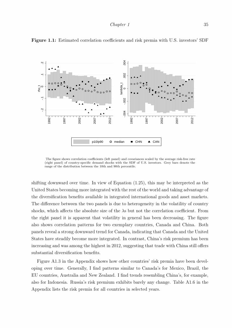
Chapter 1 35
Figure 1.1: Estimated correlation coefficients and risk premia with U.S. investors’ SDF-.
2-.
10
.1.2
rho_
t
1992
1997
2002
2007
2012
-.00
4-.
002
0.0
02.0
04la
mbd
a_t
1992
1997
2002
2007
2012
p10/p90 median CHN CAN
The figure shows correlation coefficients (left panel) and covariances scaled by the average risk-free rate(right panel) of country-specific demand shocks with the SDF of U.S. investors. Grey bars denote therange of the distribution between the 10th and 90th percentile.
shifting downward over time. In view of Equation (1.25), this may be interpreted as theUnited States becoming more integrated with the rest of the world and taking advantage ofthe diversification benefits available in integrated international goods and asset markets.The difference between the two panels is due to heterogeneity in the volatility of countryshocks, which affects the absolute size of the λs but not the correlation coefficient. Fromthe right panel it is apparent that volatility in general has been decreasing. The figurealso shows correlation patterns for two exemplary countries, Canada and China. Bothpanels reveal a strong downward trend for Canada, indicating that Canada and the UnitedStates have steadily become more integrated. In contrast, China’s risk premium has beenincreasing and was among the highest in 2012, suggesting that trade with China still offerssubstantial diversification benefits.
Figure A1.3 in the Appendix shows how other countries’ risk premia have been devel-oping over time. Generally, I find patterns similar to Canada’s for Mexico, Brazil, theEU countries, Australia and New Zealand. I find trends resembling China’s, for example,also for Indonesia. Russia’s risk premium exhibits barely any change. Table A1.6 in theAppendix lists the risk premia for all countries in selected years.

36 Global Risk Sharing Through Trade in Goods and Assets: Theory and Evidence
1.4.3 Testing the Relevance of Risk Premia in the Gravity Model
1.4.3.1 Empirical Model and Data
With the estimated risk premia in hand, I can now test the main prediction of the model,which states that firms take into account the riskiness of markets for their investors whendeciding how much to ship to a given market, as implied by Equation (1.12):
q∗jh,t =θ(1 + λjh,t)
ε(Rfj,t+1cj,tτjh,t
)−ε∑
j∈I Nj,t(1 + λjh,t)ε−1(Rfj,t+1cj,tτjh,t
)1−ε · Et [Yh,t+1]
Note that I add an index t to the cost parameters to acknowledge that they are po-tentially time varying as well. I use finely disaggregated product-level exports from theUnited States to 175 destination countries to test whether exports are, ceteris paribus,higher to countries exhibiting larger covariances with the SDF of U.S. investors.24 Thedata are from the U.S. Census Bureau’s Foreign Trade Division and cover the universeof U.S. exports. I use three equally spaced time periods between 1992 and 2012 to allowstructural changes in risk premia over time to come into effect. I consider more yearsof data in a robustness analysis. My main estimation equation is a log-linear version ofEquation (1.12),
ln qjh,t = ε ln(1 + λjh,t)− ε ln τjh,t − ε ln(Rfj,t+1cj,t
)+ ln θ + ln Et [Yh] + ln Πjh,t, (1.32)
where Πjh,t =∑
j∈I Nj,t(1 + λjh,t)ε−1(Rfj,t+1cj,tτjh,t
)1−ε. In the empirical model, j now
indicates a product and h is a destination market. My dependent variable is the quantity(in kilograms) of product j shipped to country h in year t. I use an algorithm developedby Pierce and Schott (2012) to concord a total of 12,364 HS 10-digit product categoriesfrom the original dataset over time. This yields 7,056 product groups that are robustwith respect to changes in the classification and the creation or elimination of productcategories. Export quantities and values are aggregated to the level of these syntheticproduct codes. I use shipments by air or vessel only, which make up more than 90%of value shipped for about 98% of all observations; robustness checks with regard tothis choice will be provided. Table A1.7 summarizes all variables used in the gravity
24I observe 180 destination countries in the dataset, but only for 175 of them data on all relevant variablesis available.

Chapter 1 37
estimations and contains details regarding data sources and variable definitions. Thedata appendix A1.5 provides further details.
On the right-hand side of Equation (1.32) I use logs of real GDP and real per capitaGDP to proxy for expected demand in the destination country.25 I use product-timefixed effects dj,t throughout the estimations, which absorb everything that is inherentto the product at a given point in time, but does not vary across destination markets,such as production cost, quality, or the world level of demand. These product-time fixedeffects also absorb the risk-free rate. Moreover, I include product-country fixed effectsdjh to capture market-product-specific characteristics that do not vary over time, such aspart of the trade costs and the time-constant component of country h’s degree of marketcompetition, Πjh,t, also known as multilateral resistance. For the time-varying part ofthe trade cost, I use a binary trade agreement indicator and estimates of freight cost forshipments by vessel and air. Since I do not directly observe freight cost for U.S. exports,I use data on U.S. imports by product and country of origin, also from the U.S. CensusBureau’s Foreign Trade Division, to calculate median ad valorem shipping cost by partnercountry and time, assuming that bilateral freight costs of imports are a reasonable proxyfor bilateral freight costs of exports. Since the availability of tariff data is limited, I includethem only in a robustness analysis. The empirical model used to test the model’s centralprediction is thus
ln qjUSh,t = β1 ln(1 + λUSh,t ) + β2FreightCosth,t + β3RTAh,t + β4 lnGDPh,t
+ β5 lnCGDPh,t + djh + dj,t + ujh,t. (1.33)
A potential omitted variables concern involves the fact the multilateral resistance termsΠjh,t may vary across time and products and are thus not fully captured by product-destination and product-time fixed effects. Hence, consistent estimation of the coefficientsin Equation (1.33) with OLS relies on the assumption that the time-varying componentof Πjh,t, that ends up in the error term, is uncorrelated with the regressors. The disag-gregation of the data by transportation mode, which I describe below, allows addressingthis issue.
25Given that in the presence of time lags firms base export quantities on the expected level of demand,this choice is not innocuous. But it is hard to come by a better proxy. Besides the fact that exporters’expectation are unobserved, the exact point in time at which the expectation is formed is also unknown.Note that t here denotes the point in time when the goods pass U.S. customs. If production of the goodtook a significant amount of time, the firm might have formed the relevant expectation much earlier.Some relief is provided by the fact that I look at total shipments within a year. If expectations arerational, then the sum of expected demand over subperiods of time should converge to the total realizedlevel of demand. I conduct a robustness test using GDP and GDP per capita from the previous year.

38 Global Risk Sharing Through Trade in Goods and Assets: Theory and Evidence
First, however, I consider heterogeneity of the effect of λ across sectors to assess thevalidity of the model’s key assumption, which is that the correlation pattern of demandshocks matters because of a time lag between production and sales. If firms could immedi-ately adjust quantities to the current demand level, they would still exhibit volatile profitsand thus expose their investors to risk, yet current sales would be perfectly explained bythe current level of demand and the λs should not matter. I use Rajan and Zingales’s(1998) measure of external finance dependence to differentiate sectors based on their needfor upfront investment, which is measured by the average share of capital expenditurethat cannot be financed by the cash flow from the same project. Presuming that a needfor upfront investment implies that there is a relevant time lag between production andsales, I test whether exports of products from sectors that are more dependent on upfrontinvestment are more strongly affected by the correlation pattern of country shocks bymeans of an interaction term ln(1 + λUSh,t )×ExtF inDepsj ,t. sj denotes the sector definedby the NAICS six-digit code to which product j belongs.26
Next, I consider heterogeneity across transportation modes. Products shipped by vesseland by air to the same market at the same point in time provide me with a nice opportunityto test for the relevance of a time lag caused by shipping. Arguably, air shipments areless or not at all exposed to demand volatility once the good has reached the U.S. border.To test this presumption, I estimate Equation (1.33) separately for shipments by air andshipments by vessel. As an alternative estimation strategy, I pool shipments by bothtransportation modes and assess a differential impact of λ by means of an interactionterm with a zero-one indicator for air shipment. Hence, I estimate
ln qmjUSh,t = β1 ln(1 + λUSh,t ) + β11 ln(1 + λUSh,t )× Airmjh,t + β2FreightCosth,t + β3RTAh,t
+ β4 lnGDPh,t + β5 lnCGDPh,t + djmh + djm,t + ujmh,t (1.34)
where m ∈ (Air, V es), to test whether risk premia have a differential effect on shipmentsby air relative to shipments by vessel. The disaggregation by transportation mode alsoallows me to estimate this interaction term with a specification where product-destination-time fixed effects take care of time-varying multilateral resistance terms:
ln qmjUSh,t = β11 ln(1 + λUSh,t )× Airmjh,t + djmh + djm,t + djh,t + ujmh,t (1.35)
26There are a few products where the assignment to NAICS six-digit sectors is no longer unique afteraggregating HS10 digits to time consistent product groups as described above. I use weighted averagesof the ExtFinDep measure in those cases.

Chapter 1 39
The sign of the direct effect λ on shipments by air is a priori ambiguous. Considerthe extreme case where the only cause of a time lag is transit time by vessel so thatproduction and delivery by air is possible instantly.27 Shipments by vessel, however, havethe advantage of being cheaper. In line with the logic laid out by Aizenman (2004) andHummels and Schaur (2010), firms will ship some positive quantity by vessel and wheneverdemand shocks are positive and large, they will exercise the option of shipping some moreby expensive air transport. Under these conditions, air shipments are fully explainedby the current level of demand and the quantity previously shipped by vessel. If vesselshipments are larger to markets offering diversification benefits in terms of positive λ’s,then the option value of serving those markets by air is smaller. Hence, we would expectto see a negative impact of λ on shipments by air. Arguably, the case of instant delivery isextreme. Time lags caused by production and shipping to the airport, as well as customsprocedures, are likely also relevant for shipments by air and hence imply some degree ofexposure to market-specific demand volatility. Which effect dominates is an empiricalquestion.
1.4.3.2 Results
Column (1) of Table 1.3 shows parameter estimates from the baseline specification (1.33).Estimations are based on three years of data, equally spaced between 1992 and 2012, andrely on time variation over time within product-country cells only. Unobserved product-time-specific heterogeneity is controlled for by additional fixed effects. Throughout allestimations I calculate standard errors that are robust to two-way clusters within productsand countries, as advocated by Cameron et al. (2011).
I find that the risk premia have a significantly positive effect on export quantities. Istandardized ln(1+λ) to make coefficients comparable across specifications. The standarddeviation of ln(1 + λ) is .005; hence, the non-standardized coefficient corresponding to.033 in Column (1) is 6.6. This implies that a 1% increase in 1+λ increases trade by 6.6%.In view of Figure 1.1, this means that the change of .3% in Canada’s risk premium fromthe level in 1992 to the level of 2012 has led to a decrease in trade of about 2%. ChangingChina’s risk premium in 2012 to the level of Canada’s in 2012 would result in a trade effectof similar magnitude. Note, however, that this is a partial equilibrium argument, sincethe λs are themselves decreasing functions of the amount of trade between the UnitedStates and a given destination market. Hence, the general equilibrium effect is likely to
27Alternatively, one might consider a case where production does take time but quantities do not needto be customized to a specific market.

40 Global Risk Sharing Through Trade in Goods and Assets: Theory and Evidence
be smaller in absolute terms. The structural interpretation of the estimate is helpful ingauging the plausibility of its magnitude. The theoretical gravity equation implies thatthe elasticity of export quantities with respect to the risk premia is equal to ε, where ε−1
is the elasticity of trade values with respect to trade cost. A implied trade cost elasticityof 5.6 places this estimate well inside the range typically found in the literature.28
In Column (2) I interact the risk premia with Rajan and Zingales’s sectoral measureof external financial dependence. I find a positive and significant effect of the interaction,implying that exposure to demand volatility is more important for sectors that have tomake considerable investments upfront. This lends support to the model’s assumption of atime lag. A similar conclusion can be derived from the analysis of differential effects acrossmodes of transportation. In Columns (3) and (4) I present the results from estimatingEquation (1.33) separately for shipments by vessel and by air, respectively. As discussedabove, shipments by vessel are expected to be more affected by the correlation patternof demand shocks than shipments by air, with the effect on the latter being ambiguous apriori. I find that shipments by vessel are indeed more positively and significantly affected.The estimated effect on shipments by air is also positive, but smaller and not significant.Columns (5) - (7) show the results from estimating Equations (1.34) and (1.35) basedon the same data set, pooling shipments by air and vessel.29 Column (5) shows that thedirect effect of λ is slightly smaller in the estimation based on disaggregated data, whichallows controlling for product-destination and product-time fixed effects interacted withthe mode of transportation. The negative and significant interaction terms in Columns(6) and (7) show that the differential effect of λ on shipments by air relative to shipmentsby vessel, as indicated by Columns (3) and (4), is robust to controlling for unobservedheterogeneity on a more disaggregated level. It is reassuring that the inclusion of product-destination-time fixed effects to capture, among other things, time variation in multilateralresistance terms does not affect the estimate of the interaction term. To summarize, I finda positive and significant effect of risk premia on export quantities, suggesting that firmsdo adjust relative sales across markets in accordance with investors’ desire for smoothconsumption. The differential effects across sectors and modes of transportation implythat demand volatility constitutes a risk because of a time lag between production andsales, thus lending support to the model’s key assumption.
28See, for example, Caliendo and Parro (2015). Note, however, that the estimated magnitude is sensitiveto the choice of data frequency used to calculate the covariances (see Subsection 1.4.1) and should hencebe interpreted with care.
29Hence, the number of observations is twice as large as in Columns (1), (3), and (4) where I use eithertotal shipments by product and destination or shipments by vessel, respectively, by air, only.

Chapter 1 41
Tab
le1.3:
Gravity
estimations
withrisk
prem
ia
Dep.Var.:
lnq jh,t
lnq jh,t
lnqV
esjh,t
lnqA
irjh,t
lnqm jh,t
lnqm jh,t
lnqm jh,t
lnG
DP
0.374
0.308
0.240
0.431∗∗
0.337∗
0.337∗
(0.268)
(0.266)
(0.221)
(0.198)
(0.204)
(0.204)
lnCG
DP
0.122
0.103
0.100
0.024
0.062
0.062
(0.280)
(0.285)
(0.238)
(0.227)
(0.227)
(0.227)
RTA
0.332∗∗∗
0.349∗∗∗
0.424∗∗∗
0.130
0.276∗∗∗
0.276∗∗∗
(0.096)
(0.100)
(0.114)
(0.081)
(0.073)
(0.073)
ln(1
+λ
)0.033∗∗
0.033∗∗
0.029∗∗
0.013
0.021∗
0.031∗∗
(0.015)
(0.017)
(0.013)
(0.011)
(0.011)
(0.013)
Frei
ghtC
ost
-0.788
-0.495
-0.074
-0.435
-0.276
-0.270
-0.389∗∗
(0.963)
(0.898)
(0.237)
(0.367)
(0.289)
(0.285)
(0.194)
×A
ir-0.019∗∗
-0.019∗
(0.010)
(0.010)
×Ext
Fin
Dep
0.0003∗
(0.000)
Fixed
effects
prd×
yrprd×
yrprd×
yrprd×
yrprd×
yr×air
prd×
yr×air
prd×
yr×air
prd×
cty
prd×
cty
prd×
cty
prd×
cty
prd×
cty×
air
prd×
cty×
air
prd×
cty×
air
prd×
cty×
yrObserv ation
s3,360,036
3,094,634
3,360,036
3,360,036
6,720,072
6,720,072
6,720,072
AdjustedR
20.645
0.649
0.599
0.629
0.612
0.612
0.228
S.e.
(inpa
rentheses)
robu
stto
two-way
clusters
onprod
uctan
dcoun
trylevel.Sign
ificancelevels:∗p<
0.1,∗∗p<
0.0
5,∗∗∗p<
0.0
1.

42 Global Risk Sharing Through Trade in Goods and Assets: Theory and Evidence
Tab
le1.4:
Gravity
estimations
withrisk
prem
ia:Rob
ustness
Rob
ustnesstest:
Tariffs
5yrs(∆
=5)
21yrs(∆
=1)
Exp
ortvalue
25FFpfs
FFfour
factors
Dep.Var.:
lnq jh,t
lnq jh,t
lnq jh,t
lnq jh,t
lns jh,t
lns h,t
lnq jh,t
lnq jh,t
lnG
DP
0.856∗∗
0.881∗∗
0.454∗
0.405
0.441
1.009∗∗∗
0.373
0.395
(0.388)
(0.390)
(0.264)
(0.266)
(0.356)
(0.258)
(0.268)
(0.268)
lnCG
DP
0.149
0.189
0.049
-0.043
0.217
-0.442∗
0.122
0.120
(0.398)
(0.398)
(0.275)
(0.278)
(0.370)
(0.263)
(0.280)
(0.277)
RTA
0.191
0.211∗
0.216∗∗∗
0.150∗∗
0.446∗∗∗
-0.025
0.332∗∗∗
0.326∗∗∗
(0.122)
(0.125)
(0.077)
(0.073)
(0.116)
(0.078)
(0.096)
(0.096)
Frei
ghtC
ost
-1.912
-1.831
-0.617
-0.877∗
-1.057
-1.604∗
-0.788
-0.771
(2.096)
(2.116)
(0.607)
(0.461)
(1.317)
(0.883)
(0.963)
(0.961)
ln(1
+λ
)0.080∗
0.079∗
0.025∗
0.016∗∗
0.047∗∗
0.037∗
0.033∗∗
0.043∗∗∗
(0.045)
(0.045)
(0.013)
(0.008)
(0.021)
(0.020)
(0.015)
(0.016)
ln(1
+t)
-0.886∗∗∗
(0.317)
Fixed
effects
prd×
yrprd×
yrprd×
yrprd×
yrprd×
yryr
prd×
yrprd×
yrprd×
cty
prd×
cty
prd×
cty
prd×
cty
prd×
cty
cty
prd×
cty
prd×
cty
Observation
s1,725,578
1,725,578
5,718,219
24,418,154
3,360,036
3,586
3,360,036
3,360,036
AdjustedR
20.616
0.616
0.669
0.693
0.667
0.955
0.645
0.645
S.e.
(inpa
rentheses)
robu
stto
two-way
clusters
onprod
uctan
dcoun
trylevel.Sign
ificancelevels:∗p<
0.1,∗∗p<
0.0
5,∗∗∗p<
0.0
1.

Chapter 1 43
Table 1.5: Gravity estimations with risk premia: Robustness, continued
Robustness test: Air/Ves only ex. CAN&MEX p.kg.freight cost lagged GDPDep. Var.: ln qjh,t ln qjh,t ln qjh,t ln qjh,t
ln GDP 0.360 0.367 0.400(0.264) (0.267) (0.265)
ln CGDP 0.117 0.118 0.104(0.277) (0.279) (0.283)
ln L.GDP 0.289(0.286)
ln L.CGDP 0.044(0.299)
RTA 0.323∗∗∗ 0.321∗∗∗ 0.329∗∗∗ 0.332∗∗∗(0.101) (0.101) (0.097) (0.098)
FreightCost -0.623 -0.692 -0.913(0.905) (0.933) (0.976)
FreightCost p.kg. 0.00764(0.23)
ln(1 + λ) 0.033∗∗ 0.033∗∗ 0.034∗∗ 0.028∗∗(0.015) (0.015) (0.015) (0.014)
Fixed effects prd×yr prd×yr prd×yr prd×yrprd×cty prd×cty prd×cty prd×cty
Observations 3,288,307 3,318,872 3,360,036 3,332,734Adjusted R2 0.639 0.645 0.645 0.646S.e. (in parentheses) robust to two-way clusters on product and country level. Significance levels: ∗ p < 0.1, ∗∗p < 0.05, ∗∗∗ p < 0.01.
1.4.3.3 Robustness
I conduct various tests to analyze the robustness of my results with regard to changes inthe exact specification of Equation (1.33). Results are collected in Tables 1.4 and 1.5 inthe Appendix. First, I include tariffs as additional trade cost variables. Tariff data areavailable on the HS six-digit level; for some products on higher levels of aggregation. Timeand country coverage is very patchy, even after filling in missing values with lags or leadsor weighted averages on higher levels of aggregation.30 Hence, I lose a significant share of
30I detail the procedures used to fill in missings in Appendix A1.5.

44 Global Risk Sharing Through Trade in Goods and Assets: Theory and Evidence
observations. Column (2) of Table 1.4 shows that the effect of λ in this smaller sample isstill positive and significant, but also larger. Including tariffs (Column 1) barely affects thecoefficient estimate for λ. Next, I re-estimate Equation (1.33) using more of the availableyears of data: five equally spaced time windows between 1992 and 2012 in Column (3) andall 21 years in Column (4). The effect of λ remains positive and significant. Interestingly,it decreases in magnitude as time windows become narrower. This is consistent with thepresumption that the effect of changes in the covariance pattern on exports takes sometime to phase in.
In Column (5) I use export values on the product-year-destination level as the depen-dent variable. I find a positive and significant effect of the risk premia as well. Note thatin view of Equation (1.13), this suggests that financial markets are not fully integratedacross countries; otherwise, trade shares would be independent of λ. I also estimate agravity equation on the country level, aggregating values over all products, and I findagain a positive and significant effect of the risk premia on exports (Column 6).
I also perform robustness checks with regard to choices made in the estimation ofthe risk premia. I use Fama and French’s 25 benchmark assets as an alternative set oftest assets to obtain estimates of γUS, ζUS. These portfolios are constructed based onall stocks traded on NYSE, AMEX, and NASDAQ, which are sorted two-ways by sizein terms of equity and by value (ratio of book equity to market equity). This methodof portfolio construction, described in detail in Fama and French (1993), has becomethe benchmark for measuring the performance of models in the empirical asset pricingliterature. Moreover, I use the four factor model proposed by Fama and French (2015) asan alternative to the CAPM to obtain a predicted time series of the SDF. The four factormodel uses three mean return spreads of diversified portfolios sorted by size (RSMB), byprofitability (RRMW ), and by investment levels (RCMA) in addition to the return on themarket portfolio to describe the SDF as
mi,t+1 = ζi,t + γi,tRWi,t + γSMB
i,t RSMBi,t + γRMW
i,t RRMWi,t + γSMB
i,t RCMAi,t . (1.36)
This model is very successful in explaining the cross-section of mean asset returns, but itdoes not have a theoretical foundation. Table A1.8 presents the parameter estimates usingthe alternative test assets or the alternative SDF model, obtained from GMM estimationas decribed in Subsection 1.4.1. Changing the test assets has only a small impact onthe CAPM estimates. Similarly, adding the additional explanatory factors as prescribedby Equation (1.36) to the linear model of the SDF slightly increases the estimate of γi,tbut does not affect its significance. The other factors are not individually significant. I

Chapter 1 45
use those alternative parameter estimates to predict time series of the SDF and obtainalternative sets of country risk premia. Columns (7) and (8) of Table 1.4 show that theresults from the gravity estimation are robust to those variations.
Table 1.5 contains some additional robustness tests. Column (1) shows estimates basedon a sample from which I dropped observations for which the share of shipments (in termsof value) by a transportation mode other than air or vessel exceeds 10%. This is the casefor about 2% of all observations. In Column (2) I dropped Canada and Mexico, sinceground transportation is a relevant alternative shipping mode for contiguous countries.Shipments by vessel and air might reflect extraordinary circumstances. In Column (3)I use freight cost per kilogram instead of ad valorem freight cost and in Column (4)I use lagged values of GDP and per capita GDP as proxies for the expected level ofdemand. None of these changes to the baseline specification much affects the magnitudeor significance of the coefficient estimate for λ.
1.5 Conclusion
Trade’s potential for global risk sharing has long been understood, but supportive empir-ical evidence is rare. Following Backus and Smith (1993), a large literature has shownthat the aggregate implications of effective global risk sharing are not borne out by thedata. Financial market data show that asset markets continue to be fairly disintegrated(Fama and French, 2012). Nevertheless, competitive firms strive to maximize shareholdervalue conditional on the level of frictions inhibiting trade of goods and assets on globalmarkets. With risk-averse investors who desire high returns but also smooth consumptionover time, this implies optimization of a risk-return tradeoff for every project involvingaggregate risk.
In this paper I propose a general equilibrium model of trade in goods and investmentin assets that incorporates this logic. I show that irrespective of the degree of financialmarket integration, shareholder value maximization incentivizes to firms to take intoaccount whether volatility inherent to profits from exporting helps investors diversify therisk of volatile consumption when choosing optimal quantities. The model predicts thatfirms ship more to markets where profits tend to be high in times when investors’ othersources of income do not pay off very well. Aggregation of individual firms’ and investors’optimal choices in turn determines the amount of aggregate risk that is taken on bythe agents of the model in equilibrium, as well as the extent to which country-specificproductivity shocks that determine exporting firms’ profits contribute in a positive ornegative way to the consumption smoothing of investors from other countries.

46 Global Risk Sharing Through Trade in Goods and Assets: Theory and Evidence
Using data on returns to firm shares traded on the U.S. financial market, I estimatecorrelations of country-specific shocks with marginal utility growth of U.S. investors forthe years 1992 to 2012. The correlations indicate that over the course of three decades,the United States has become increasingly integrated with the rest of the world, with aconsequent decrease in diversification benefits from trade. In a separate analysis based onproduct-destination market export data for the United States, I show that the differentialchange in the correlation pattern across countries is consistent with long-term changes inthe pattern of trade across destination markets within narrowly defined product categories.
I conclude from this analysis that risk diversification through trade matters at the levelof the individual firm and has shaped trade patterns during the past three decades.

Appendix A.1
A1.1 Model Details
Investors’ optimization problem. The investor’s optimization problem is
max{ai,t+s,afi,t+s}∞s=0
Et∞∑s=0
ρsui(Ci,t+s)
s.t. Ci,t+s = Wi,t+s − Ai,t+sWi,t+s = RW
t+sAt+s−1 = a′i,t+s−1πit+s + afi,t+s−1R
ft+s
Ai,t+s = a′i,t+svit+s + afi,t+s
0 = lims→∞
ρsu′i(Ci,t+s)Ai,t+s
Inserting constraints (1)-(3) yields
max{ai,t+s,afi,t+s}∞s=0
Et∞∑s=0
ρsui
(a′i,t+s−1π
it+s + afi,t+s−1R
fi,t+s − a′i,t+svit+s − a
fi,t+s
)(A1.1)
s.t. 0 = lims→∞
ρsu′i(Ci,t+s)Ai,t+s
The investor’s FOCs with respect to investment (1.5) and (1.6) are readily derived fromthis expression.
Derivation of Equation (1.19). To derive Equation (1.19), I first restate the relevantequilibrium conditions for easier reference.
- Investors’ first-order conditions (1.5) and (1.6):
afi,t
[mi,t+1, R
fi,t+1
]and aij,t [vj,t, πj,t+1, mi,t+1] ∀ j ∈ Ii and i = 1, ..., ι
- Stochastic discount factor (1.8): mi,t+1
[Ci,t, Ci,t+1
]∀ i = 1, ..., ι
- Budget constraint (1.3): Ci,t
[afi,t,ai,t,v
it;Wi,t
]and
Ci,t+1
[afi,t,ai,t, π
it+1, a
fi,t+1, ai,t+1, v
it+1, R
fi,t+1
]∀ i = 1, ..., ι
Substituting Ci,t, Ci,t+1 in mi,t+1 from the budget constraint yields
mi,t+1
[afi,t,ai,t,v
it, v
it+1, π
it+1, a
fi,t+1, ai,t+1,Wi,t, R
fi,t+1
]

48 Global Risk Sharing Through Trade in Goods and Assets: Theory and Evidence
and substituting mi,t+1 in the Euler equations then gives
afi,t
[ai,t,v
it, v
it+1, π
it+1, a
fi,t+1, ai,t+1,Wi,t, R
fi,t+1
]and
aij,t
[afi,t,ai,t,v
it, v
it+1, π
it+1, a
fi,t+1, ai,t+1,Wi,t, R
fi,t+1
]∀ j ∈ Ii.
This system of Ii + 1 equations can be used to eliminate afi,t,ai,t on the “right-hand side,”so that
afi,t
[vit, v
it+1, π
it+1, a
fi,t+1, ai,t+1,Wi,t, R
fi,t+1
]and
aij,t
[vit, v
it+1, π
it+1, a
fi,t+1, ai,t+1,Wi,t, R
fi,t+1
]∀ j ∈ Ii.
Updating afi,t,ai,t one period then gives
afi,t+1
[vit+1, v
it+2, π
it+2, a
fi,t+2, ai,t+2, Wi,t+1, R
fi,t+2
]and
aij,t+1
[vit+1, v
it+2, π
it+2, a
fi,t+2, ai,t+2, Wi,t+1, R
fi,t+2
]∀ j ∈ Ii.
Replacing Wi,t+1 with afi,t,ai,t, πit+1, R
fi,t+1 and using again the system of Ii + 1 equations
to eliminate afi,t,ai,t, I obtain
afi,t+1
[vit+2, π
it+2, a
fi,t+2, ai,t+2, π
it+1, R
fi,t+1, R
fi,t+2
]and (A1.2)
aij,t+1
[vit+2, π
it+2, a
fi,t+2, ai,t+2, π
it+1, R
fi,t+1, R
fi,t+2
]∀ j ∈ Ii.
Inserting afi,t,ai,t, afi,t+1, ai,t+1 (before substituting for Wi,t+1) into mi,t+1 then yields
mi,t+1
[vit+1, v
it+2, π
it+1, π
it+2, a
fi,t+2, ai,t+2,Wi,t, Wi,t+1, R
fi,t+1, R
fi,t+2
]Now, repeated substitution of afi,t+1, ai,t+1 as in Equation (A1.2) updated to period t+ s
for s = 2, ...,∞ in mi,t+1 gives
mi,t+1
[Wi,t, Wi,t+1, {vit+s}∞s=1, {π
it+s}∞s=1, {R
fi,t+s}∞s=1
]which is equivalent to Equation (1.19) in the main text.
Derivation of Equation (1.21). Writing out in full the expection in Equation (A1.1) attime t, I obtain

Chapter 1 49
max{ai,t+s,afi,t+s}∞s=0
∞∑s=0
ρs∫ψt+s
u(a′i,t+s−1π
it+s(Ψt+s) + afi,t+s−1R
fi,t+s (A1.3)
−a′i,t+svit+s(Ψt+s)− afi,t+s)dF (ψt+s|Ψt+s−1)
s.t. 0 = lims→∞
ρsu′i(Ci,t+s)Ai,t+s
where Ψt+s denotes the full history of realized productivity levels up to t+s. Note that atthis point, no assumptions have been imposed on the distribution dF (ψt+s|Ψt+s−1) otherthan finiteness of expected values and non-negative support. As Fama (1970) showed,the problem is greatly simplified if the random variables follow independent and identicaldistribution over time. The i.i.d. assumption implicit in Equation (1.20) implies thatF (ψt+s|Ψt+s−1) = F (ψ). Moreover, the assumption that the investor takes as given thenumber of firms and the prices of the currently available set of assets (including the risk-free rate) implies that {πt+s(Ψ)}∞s=1 = πt(ψ), {vit+s(Ψ)}∞s=1 = vit, and R
ft+s = Rf
t ∀s =
1, ...,∞, that is, profits associated with a given realization of ψ and asset prices areexpected not to change over time.31 Then, given the current state of the economy t, theinvestor’s optimization problem at any future date t+ s is identical to the problem facedat time t except for the level of wealth Wi,t+s he is starting with. Let G(Wt) denote themaximum value of the optimization problem (A1.3) as a function of the initial level ofwealth. Then, (A1.3) may be written as
max{ai,t+s}∞s=0
ui(Wi,t − a′i,tvt − afi,t+1) + ρG(Wi,t+1)
s.t. 0 = lims→∞
ρsu′i(Ci,t+s)Ai,t+s
and the first order conditions obtain as
1 = Et[ρG′(Wi,t+1)
u′i(Ci,t)
]Rfi,t+1 and vj,t = Et
[ρG′(Wi,t+1)
u′i(Ci,t)(πj,t+1 + vj,t+1)
]∀ j, t.
Hence, the SDF observes
mi,t+1 = ρG′(Wi,t+1)
u′i(Ci,t)= ρ
G′(RWi,t+1(Wi,t − Ci,t)
)u′i(Ci,t)
= gi,t(RWi,t+1).
Under the lognormal assumption on productivity levels (Equation (1.20)), returns tofirm shares as described in Equation (1.18) and the return to the wealth portfolio (Equa-
31Equation (A1.3) implies that ψ is the only source of uncertainty. However, including uncertainty aboutchanges in exogenous variables as well does not affect the investor’s choice problem if shocks are i.i.d.and independent of Ψ.
50 Global Risk Sharing Through Trade in Goods and Assets: Theory and Evidence
tion (1.4)) are approximately normally distributed. Using Stein’s Lemma, I obtain anapproximate linear relationship between the SDF and the return to the wealth portfolio.The following derivation closely follows Cochrane (2005), Chapter 9.
Stein’s Lemma: If f,R are bivariate normal (BVN), g(f) is differentiable andE[|g′(f)|] <∞, then Cov[g(f), R] = E[g′(f)]Cov[f,R].
Now, assume Et[∣∣g′i,t(RW
i,t+1)∣∣] < ∞. Then, RW
i,t+1 and Rj,t+1 ∼approx.
BVN ∀ j ∈ Ii,
mi,t+1 = gi,t(RWi,t+1), the investor’s first-order conditions
1 = Et[mi,t+1Rj,t+1] ⇔ 1 = Et[mi,t+1]Et[Rj,t+1] + Covt[mi,t+1, Rj,t+1], (A1.4)
and Stein’s lemma imply that
1 = Et[gi,t(RWi,t+1)]Et[Rj,t+1] + Et[g′i,t(R
Wi,t+1)]Covt[RW
i,t+1, Rj,t+1].
Hence, a SDF of the formmi,t+1 = Et[gi,t(RWi,t+1)]+Et[g′i,t(RW
i,t+1)](RWi,t+1−Et[RW
i,t+1]) existsthat is linear in RW
i,t+1 and satisfies Equation (A1.4) for all j ∈ Ii.
A1.2 Current Account and Balance of Payments
The current account of country k ∈ Ii defined as net exports plus net earnings fromforeign investment obtains as the sum of final goods net exports Yk,t + afk,t−1R
fk,t −(
Ck,t +∑
j∈Ii akj,tvj,t + afk,t +Nk,tvk,t
)(final goods output including savings minus do-
mestic absorption), net domestic intermediate exports Nk,t−1
∑h∈I φkh,t−1Yh,t − Yk,t (ex-
ports by variety producers minus intermediate imports by final goods producers) andprofits owned from investment in foreign assets
∑j∈Ii akj,t−1πj,t minus profits owned by
foreign investors in the home country Nk,t−1πk,t.32 The current account is then
CAk,t = Yk,t + afk,t−1Rfk,t −
(Ck,t +
∑j∈Ii
akj,tvj,t + afk,t +Nk,tvk,t
)+Nk,t−1
∑h∈I
φkh,t−1Yh,t − Yk,t +∑j∈Ii
akj,t−1πj,t −Nk,t−1πk,t
= −∑j∈Ii
dakj,tvj,t + dNkvk,t
32I include domestic sales and domestic earnings in inflows and outflows to save on notation. They neteach other out in all positions.

Chapter 1 51
and equal to net foreign investment, that is, equal to the capital account. Hence, theinternational payment system is balanced.
A1.3 Expected Return-Beta Representation
The structural equation of the SDF (1.22) falls into the class of linear factor models, whichare commonly used in the asset pricing literature to analyse asset returns by means oftheir correlations with factors, typically portfolio returns or macro variables. In my casethe factors are country-specific productivity shocks. As shown in Cochrane (1996), everylinear factor model has an equivalent expected return-beta representation which impliesthat the λs can be interpreted as monetary factor risk premia or factor prices.
The Euler equation for risky assets (1.6) implies that, in equilibrium, the return toevery asset j ∈ Ii observes
1 = Et [mi,t+1Rj,t+1] where mi,t+1 = bi0,t + b′i,tY t+1.
Following Cochrane (2005) Chapter 6, I can rewrite this as
Et [Rj,t+1]−Rfi,t+1 = −Rf
i,t+1b′i,tCovt
[Y t+1, Rj,t+1
](A1.5)
= −Rfi,t+1b
′i,tCovt
[Y t+1, Y
′t+1
]Covt
[Y t+1, Y
′t+1
]−1
Covt[Y t+1, Rj,t+1
].
Define βj,t := Covt[Y t+1, Y
′t+1
]−1
Covt[Y t+1, Rj,t+1
]as the vector of coefficients result-
ing from a multivariate time-series regression of firm j’s return on the factors. Then,Equation (1.24) implies that (A1.5) can be written as
Et [Rj,t+1]−Rfi,t+1 = −λ′i,tβj,t.
A1.4 A Special Case of λ = 0
To show that λt = 0 and Et [ψh,t+1] ≥ Et [ψi,t+1] imply that the number of firms in countryi is weakly larger, I consider the amount of composite good production consistent withfirms’ optimal quantity decisions as given in Equation (1.12) evaluated at λt = 0:
Qi,t =
(∑j=i,h
Nj(q∗j,i)
ε−1ε
) εε−1
= θEt [Yi,t+1](Nic
1−ε +Nh(cτ)1−ε) εε−1
Since Et [Yh,t+1] = Et [Yi,t+1], Qi,t ≥ Qh,t implies Nic1−ε+Nh(cτ)1−ε ≥ Ni(cτ)1−ε+Njc
1−ε.This holds true if Ni ≥ Nh and it means that market i is more competitive since it featuresa larger number of domestic firms that do not incur trade costs to access the market

52 Global Risk Sharing Through Trade in Goods and Assets: Theory and Evidence
compared to country h where the number of foreign firms is larger than the number ofdomestic firms. Comparing optimum firm values as given in (1.14) evaluated at λt = 0,shows that
V ∗h,t − V ∗i,t =Et [Yh,t+1]
Rft+1
(ψhh,t + ψhi,t − ψii,t − ψih,t)
=Et [Yh,t+1]
Rft+1
(1− τ 1−ε)
(1
Niτ 1−ε +Nj
− 1
Ni +Njτ 1−ε
)≥ 0. (A1.6)
Hence, the only case where the free entry condition is not violated is the knife-edge caseEt [ψh,t+1] = Et [ψi,t+1].
A1.5 Data Appendix
Import growth. I use total monthly imports by country obtained from the IMF’sDirection of Trade Database to measure demand growth. Imports are converted to con-stant U.S. dollars using the Bureau of Labor Statistics’ monthly consumer price index.Growth is measured with respect to the previous month and rates are adjusted for con-stant monthly factors. The earliest observation used to estimate the covariance matrixof import growth across countries is January 1983. To obtain continous import series forcountries evolving from the break-up of larger states or country aggregates defined by theIMF, I use a proportionality assumption to split imports reported for country groups. Inparticular, I use each country’s share in the total group’s import in the year succedingthe break up to split imports among country group members in all years before the breakup. This concerns member countries of the former USSR, Serbia and Montenegro, theSocialist Federal Republic of Yugoslavia, Belgium and Luxembourg, former Czechoslo-vakia, and the South African Common Customs Area. Moreover, I aggregate China andTaiwan, Westbank and Gaza, as well as Serbia and Kosovo in order to accommodate thereporting levels of other data used in the analysis.
Tariffs. Source: WITS database. I use effectively applied tariffs including ad valoremequivalents of specific tariffs and quotas. Tariffs are provided mostly on HS six-digit level.I use trade weighted averages on the four-digit and two-digit levels to fill missing. Thereby,I obtain tariffs for 27% of all export observations. Filling missings with up to three lags orleads yields non-missing tariffs for another 15% of the sample. There are a few productswhere the assignment to HS six-digit sectors is no longer unique after aggregating HSten-digits to time consistent product groups as described above. I use weighted averagesof tariffs in those cases where weights correspond to the number of products in potentiallydifferent HS 6 groups.
Freight costs. Source: U.S. Census FTD import data provided by Peter Schott throughhis website at http://faculty.som.yale.edu/peterschott/sub_international.htm. I compute

Chapter 1 53
median freight cost per unit value or per kg for total shipments and by mode of trans-portation on the country-year level.

54 Global Risk Sharing Through Trade in Goods and Assets: Theory and Evidence
Figure A1.1: Common risk factors used to adjust cash flows or discount rates.
0 20 40 60 80
Percent of CFOs who always or almost always adjust for a given risk
Momentum
Market-to-book ratio
Distress
Term structure
Commodity price
Size
Unexpected inflation
GDP or business cycle
Foreign exchange
Interest rate
Market risk
Source: Figure 4 in Graham and Harvey (2001)

Chapter 1 55
Figure A1.2: Mean excess return of 49 value-weighted portfolios
AgricFoodSodaBeer
SmokeToysFun
BooksHshldClthsHlth
MedEqDrugs
ChemsRubbr
TxtlsBldMtCnstrSteel
FabPrMachElcEqAutosAero
ShipsGunsGold
MinesCoal
OilUtil
TelcmPerSvBusSvHardwSoftwChips
LabEqPaperBoxesTransWhlslRtail
MealsBanks
InsurRlEst
FinOther
Indu
stry
por
tfolio
s
-4 -3 -2 -1 0 1 2 3 4in %
mean return
33th to 67th percentile range
Mean excess return over risk-free rate (U.S.t-bill rate) calculated over monthlyobservations between January 1977 and July 2014.

56 Global Risk Sharing Through Trade in Goods and Assets: Theory and Evidence
Figure A1.3: Risk premia estimates for selected countries
-.00
4-.
002
0.0
02.0
04la
mbd
a_t
1992 1997 2002 2007 2012
DEU BRA JPN
MEX RUS GHA

Chapter 1 57
Table A1.6: Estimated country risk premia for selected years
Country ISO λUSh,1992 λUSh,2002 λUSh,2012
Afghanistan AFG -0.0063 -0.0020 -0.0007Angola AGO -0.0019 -0.0051 0.0014Albania ALB 0.0048 -0.0018 -0.0001Netherlands Antilles ANT 0.0031 -0.0020 -0.0044United Arab Emirates ARE -0.0006 -0.0000 -0.0007Argentina ARG 0.0012 -0.0011 -0.0010Armenia ARM -0.0043 -0.0064 -0.0033Australia AUS 0.0016 -0.0010 -0.0028Austria AUT 0.0007 0.0001 -0.0010Azerbaijan AZE 0.0007 0.0015 -0.0031Burundi BDI 0.0020 -0.0004 0.0007Belgium BEL 0.0017 -0.0005 -0.0016Benin BEN 0.0023 0.0007 -0.0022Burkina Faso BFA 0.0050 -0.0013 -0.0002Bangladesh BGD 0.0046 -0.0010 -0.0002Bulgaria BGR -0.0026 -0.0003 -0.0003Bahrain BHR -0.0019 0.0024 -0.0018Bahamas, The BHS 0.0007 -0.0104 0.0022Bosnia and Herzegovina BIH 0.0015 0.0010 -0.0004Belarus BLR -0.0006 -0.0010 -0.0024Belize BLZ 0.0018 -0.0001 -0.0022Bermuda BMU -0.0051 0.0107 0.0006Bolivia BOL -0.0024 -0.0008 0.0006Brazil BRA 0.0029 0.0007 -0.0014Barbados BRB -0.0006 0.0010 -0.0003Brunei Darussalam BRN -0.0047 -0.0004 -0.0020Central African Republic CAF 0.0028 0.0022 -0.0157Canada CAN 0.0017 -0.0014 -0.0013Switzerland CHE 0.0015 -0.0007 0.0001Chile CHL -0.0012 0.0004 -0.0014China CHN -0.0006 0.0003 0.0014Cote d’Ivoire CIV 0.0009 0.0005 0.0041Cameroon CMR -0.0014 0.0009 -0.0011Congo, Rep. COG 0.0031 -0.0050 0.0047Colombia COL -0.0003 -0.0021 -0.0007Comoros COM -0.0041 0.0022 0.0055Cabo Verde CPV 0.0025 -0.0153 -0.0040Costa Rica CRI 0.0022 -0.0004 -0.0016Cuba CUB -0.0012 0.0001 -0.0006Cyprus CYP 0.0002 -0.0009 -0.0012Czech Republic CZE -0.0014 -0.0003 0.0000Germany DEU 0.0010 -0.0003 -0.0008Djibouti DJI 0.0000 0.0004 -0.0014Dominica DMA 0.0009 -0.0043 -0.0062Denmark DNK 0.0008 -0.0007 -0.0007Dominican Republic DOM -0.0001 -0.0011 -0.0021Algeria DZA 0.0002 0.0006 -0.0000Ecuador ECU -0.0020 -0.0004 0.0005Egypt, Arab Rep. EGY 0.0022 0.0031 0.0004Spain ESP 0.0021 0.0010 -0.0005Estonia EST -0.0012 -0.0002 -0.0015Ethiopia ETH 0.0111 -0.0016 0.0008Finland FIN 0.0024 0.0007 -0.0009Fiji FJI 0.0000 0.0014 -0.0030France FRA 0.0020 -0.0008 -0.0009Faeroe Islands FRO 0.0013 -0.0025 -0.0013Gabon GAB -0.0022 -0.0016 0.0006United Kingdom GBR 0.0005 -0.0008 -0.0002Georgia GEO -0.0008 -0.0037 -0.0005Ghana GHA -0.0016 0.0017 -0.0004Guinea GIN 0.0027 0.0012 -0.0011Gambia, The GMB 0.0045 0.0035 -0.0002Guinea-Bissau GNB -0.0006 -0.0139 0.0089Equatorial Guinea GNQ -0.0100 0.0037 -0.0056Greece GRC 0.0028 0.0011 -0.0002Grenada GRD 0.0026 -0.0053 -0.0001Greenland GRL -0.0022 -0.0007 -0.0066Guatemala GTM 0.0012 -0.0024 0.0007Guyana GUY -0.0021 0.0023 0.0026Hong Kong SAR, China HKG -0.0004 0.0003 0.0003
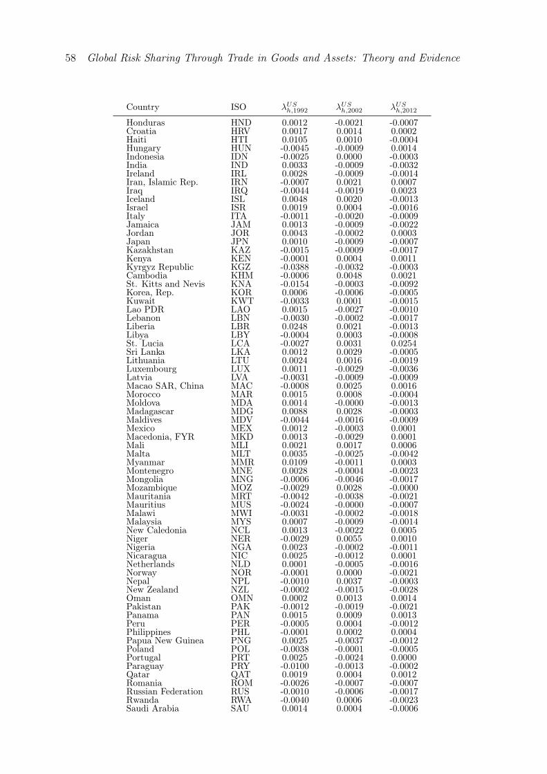
58 Global Risk Sharing Through Trade in Goods and Assets: Theory and Evidence
Country ISO λUSh,1992 λUSh,2002 λUSh,2012
Honduras HND 0.0012 -0.0021 -0.0007Croatia HRV 0.0017 0.0014 0.0002Haiti HTI 0.0105 0.0010 -0.0004Hungary HUN -0.0045 -0.0009 0.0014Indonesia IDN -0.0025 0.0000 -0.0003India IND 0.0033 -0.0009 -0.0032Ireland IRL 0.0028 -0.0009 -0.0014Iran, Islamic Rep. IRN -0.0007 0.0021 0.0007Iraq IRQ -0.0044 -0.0019 0.0023Iceland ISL 0.0048 0.0020 -0.0013Israel ISR 0.0019 0.0004 -0.0016Italy ITA -0.0011 -0.0020 -0.0009Jamaica JAM 0.0013 -0.0009 -0.0022Jordan JOR 0.0043 -0.0002 0.0003Japan JPN 0.0010 -0.0009 -0.0007Kazakhstan KAZ -0.0015 -0.0009 -0.0017Kenya KEN -0.0001 0.0004 0.0011Kyrgyz Republic KGZ -0.0388 -0.0032 -0.0003Cambodia KHM -0.0006 0.0048 0.0021St. Kitts and Nevis KNA -0.0154 -0.0003 -0.0092Korea, Rep. KOR 0.0006 -0.0006 -0.0005Kuwait KWT -0.0033 0.0001 -0.0015Lao PDR LAO 0.0015 -0.0027 -0.0010Lebanon LBN -0.0030 -0.0002 -0.0017Liberia LBR 0.0248 0.0021 -0.0013Libya LBY -0.0004 0.0003 -0.0008St. Lucia LCA -0.0027 0.0031 0.0254Sri Lanka LKA 0.0012 0.0029 -0.0005Lithuania LTU 0.0024 0.0016 -0.0019Luxembourg LUX 0.0011 -0.0029 -0.0036Latvia LVA -0.0031 -0.0009 -0.0009Macao SAR, China MAC -0.0008 0.0025 0.0016Morocco MAR 0.0015 0.0008 -0.0004Moldova MDA 0.0014 -0.0000 -0.0013Madagascar MDG 0.0088 0.0028 -0.0003Maldives MDV -0.0044 -0.0016 -0.0009Mexico MEX 0.0012 -0.0003 0.0001Macedonia, FYR MKD 0.0013 -0.0029 0.0001Mali MLI 0.0021 0.0017 0.0006Malta MLT 0.0035 -0.0025 -0.0042Myanmar MMR 0.0109 -0.0011 0.0003Montenegro MNE 0.0028 -0.0004 -0.0023Mongolia MNG -0.0006 -0.0046 -0.0017Mozambique MOZ -0.0029 0.0028 -0.0000Mauritania MRT -0.0042 -0.0038 -0.0021Mauritius MUS -0.0024 -0.0000 -0.0007Malawi MWI -0.0031 -0.0002 -0.0018Malaysia MYS 0.0007 -0.0009 -0.0014New Caledonia NCL 0.0013 -0.0022 0.0005Niger NER -0.0029 0.0055 0.0010Nigeria NGA 0.0023 -0.0002 -0.0011Nicaragua NIC 0.0025 -0.0012 0.0001Netherlands NLD 0.0001 -0.0005 -0.0016Norway NOR -0.0001 0.0000 -0.0021Nepal NPL -0.0010 0.0037 -0.0003New Zealand NZL -0.0002 -0.0015 -0.0028Oman OMN 0.0002 0.0013 0.0014Pakistan PAK -0.0012 -0.0019 -0.0021Panama PAN 0.0015 0.0009 0.0013Peru PER -0.0005 0.0004 -0.0012Philippines PHL -0.0001 0.0002 0.0004Papua New Guinea PNG 0.0025 -0.0037 -0.0012Poland POL -0.0038 -0.0001 -0.0005Portugal PRT 0.0025 -0.0024 0.0000Paraguay PRY -0.0100 -0.0013 -0.0002Qatar QAT 0.0019 0.0004 0.0012Romania ROM -0.0026 -0.0007 -0.0007Russian Federation RUS -0.0010 -0.0006 -0.0017Rwanda RWA -0.0040 0.0006 -0.0023Saudi Arabia SAU 0.0014 0.0004 -0.0006

Chapter 1 59
Country ISO λUSh,1992 λUSh,2002 λUSh,2012
Sudan SDN 0.0034 -0.0013 0.0018Senegal SEN 0.0009 0.0007 -0.0038Singapore SGP 0.0002 -0.0008 0.0001Solomon Islands SLB -0.0001 0.0006 0.0022Sierra Leone SLE 0.0023 0.0090 0.0001El Salvador SLV 0.0009 -0.0014 0.0016Somalia SOM 0.0030 -0.0024 -0.0007Serbia SRB 0.0022 -0.0004 -0.0006Sao Tome and Principe STP 0.0068 0.0405 0.0026Suriname SUR -0.0025 -0.0005 0.0003Slovak Republic SVK -0.0016 0.0012 0.0002Slovenia SVN 0.0009 0.0000 0.0002Sweden SWE 0.0008 -0.0048 -0.0013Seychelles SYC -0.0322 -0.0046 0.0056Syrian Arab Republic SYR 0.0047 -0.0021 -0.0010Chad TCD 0.0027 0.0047 0.0026Togo TGO -0.0001 -0.0060 0.0046Thailand THA 0.0006 -0.0031 -0.0002Tajikistan TJK 0.0003 -0.0029 -0.0021Turkmenistan TKM -0.0001 0.0034 0.0006Tonga TON 0.0041 -0.0010 -0.0066Trinidad and Tobago TTO -0.0026 0.0038 -0.0024Tunisia TUN 0.0013 -0.0013 -0.0011Turkey TUR 0.0012 -0.0007 -0.0015Tanzania TZA 0.0024 0.0010 -0.0000Uganda UGA 0.0013 -0.0013 -0.0016Ukraine UKR -0.0003 -0.0027 0.0003Uruguay URY 0.0028 -0.0041 -0.0013United States USA 0.0010 0.0006 -0.0010Uzbekistan UZB 0.0019 -0.0041 -0.0017St. Vincent and the Grenadines VCT -0.0057 -0.0062 -0.0053Venezuela, RB VEN 0.0013 -0.0026 -0.0028Vietnam VNM -0.0037 -0.0012 -0.0014Vanuatu VUT -0.0158 -0.0144 -0.0514Samoa WSM 0.0030 0.0170 0.0047Yemen, Rep. YEM 0.0002 0.0022 -0.0013South Africa ZAF 0.0017 -0.0011 -0.0004Congo, Dem. Rep. ZAR -0.0012 -0.0027 -0.0018Zambia ZMB -0.0015 -0.0006 -0.0039Zimbabwe ZWE 0.0034 0.0034 -0.0052

60 Global Risk Sharing Through Trade in Goods and Assets: Theory and Evidence
Tab
leA1.7:
Summarystatistics
ofvariab
lesused
inthegrav
ityestimations
Exp
ortda
taDescription
#Obs.
#Group
sMean
Std.
Dev.
Min
Max
Source,no
tes
Value
3,681,276
650,132
26,504,289
01.56
e+10
USCensus,
FTD;cp.
Qua
ntity
inkg
.3,681,276
339,153
30,258,985
02.75e+
10Piercean
dScho
tt(2012a)
#Years
3,681,276
31992
2012
#Markets
3,681,276
180
#Produ
cts
timeconsistent
HS1
0digits
3,681,276
7061
cp.Piercean
dScho
tt(2012b
)or
derivedcodes
Markets
p.product
withpo
sitive
sales
811,408
6132
1179
Produ
ctsp.
market
withpo
sitive
sales
811,408
3,150
1,480
25,831
Qua
ntityp.
market
excl.zeros,
inkg
.811,408
1,538,702
2,148,113
5,924
9,802,089
Airshare
811,408
.38
.45
01
Exp
orts
byvessel
Markets
p.product
withpo
sitive
sales
3,681,276
2824
0166
Qua
ntityp.
market
excl.zeros,
inkg
.579,516
2,143,041
3,768,501
14,781
55113832
Exp
orts
byair
Markets
p.product
withpo
sitive
sales
509,459
5233
1178
Qua
ntityp.
market
excl.zeros,
inkg
.509,459
12,932
12,576
205
50,000
Cou
ntry
data
λ3,681,276
533
-0.0004
0.0050
-0.0514
0.0405
GDP
3,536,232
512
1.83e+
115.40e+
111.08e+
84.71e+
12W
DI,PW
TCGDP
3,536,232
512
9,746
14,703
114
79,782
WDI,PW
TRTA
3,681,276
533
0.05
0.21
0.00
1.00
WTA
RTA
databa
seFreightC
ost
bycoun
try,
advalorem×
year
3,646,760
528
0.07
0.04
0.00
0.59
USCen
sus,
FTD
(impo
rtda
ta)
byair
bycoun
try×
year,ad
valorem
3,605,346
522
0.08
0.06
0.00
0.57
USCensus,
FTD
(impo
rtda
ta)
byvessel
bycoun
try×
year,ad
valorem
3,605,332
522
0.07
0.07
0.00
0.99
USCensus,
FTD
(impo
rtda
ta)
Tariff
byHS6×
coun
try×
year,ad
valorem
1,954,321
91,415
0.20
0.67
0.00
30.00
WIT
S
Sector
data
ExtFinDep
byNAIC
S6digittimes
year
3,296,991
1,437
-0.12
5.58
-93.16
33.51
Com
pustat;cp.
Rajan
andZingales(1998)

Chapter 1 61
Table A1.8: Parameter estimates of linear SDF models
Model: CAPM FF four factor modelTest assets: 25 FF pfs. 49 industry portfolios
ζUS 1 1[119] [76.7]
γUS -3.77 -4.22[-2.7] [-2.3]
γsmbUS 3.21[1.13]
γrmwUS -7.92[-1.24]
γcmaUS 4.57[.74]
# Moment Conditions 26 50# Observations 450 450# Parameters 2 5
Test of joint signific.: χ2e 131 1853
P(χ22 > χ2
e) 0 0J-Test: J-Stat 131 67P(χ2
M−k > J) 0 .02
Results from first-stage GMM. Time period: 1977M1–2014M6. t-statistics inbrackets. Column (1) uses Fama and French (1993)’s 25 Benchmark portfolios(and the risk-free rate) as test assets. Column (2) based on Fama and French(2015)’s four factor model and 49 value-weighted industry portfolios. k denotes# parameters and M # of moment conditions.


Chapter 2
Heterogeneous Workers, Trade, andMigration∗
2.1 Introduction
Workers are a heterogeneous lot. They have different innate abilities and choose differ-ent types and levels of skill formation. The outcome is both vertical and horizontal skilldifferentiation among workers. Economic well-being depends on good matches betweenworkers’ skills and their employment in different activities or firms. Obviously, the qual-ity of these matches is determined by labor market institutions. Less obviously, it alsodepends on whether economies are connected to each other by trade and migration. Inthis paper, we analyze how horizontal skill heterogeneity among workers impacts on thewelfare and inequality effects of trade and migration.
We develop a general equilibrium model of trade and migration where workers differin terms of their specific skills. By skills, we mean an individual’s relative ability toperform different types of tasks. By specificity, we mean that a certain pattern of suchtask-related abilities will be particularly useful for a certain product (or industry), andless so for others. Thus, for any given product there is a unique ideal pattern of task-related abilities, which we simply call the ideal skill type. The more a worker’s specificabilities deviate from this ideal skill type, the lower her productivity when employed by afirm producing this product. We focus on horizontal skill heterogeneity in assuming thatall workers have the same absolute level of skills, but feature different relative abilities,
∗This chapter is coauthored by Wilhelm Kohler. An earlier version was published as CESifo WorkingPaper No. 4387, 2013. The chapter extends, generalizes, and formalizes ideas developed in my Master’sthesis (submitted under the same title in 2011).
64 Heterogeneous Workers, Trade, and Migration
i.e., different skill types. Moreover, we assume that both, the absolute level of skills andthe degree of heterogeneity in skill types across workers is given exogenously, whetherinnately or from past educational investment.
We highlight two problems deriving from such worker heterogeneity. First, if the num-ber of different skill types is large and if production involves a fixed cost, then the economyfaces a matching problem. There will not be enough entry of firms for each worker to findfor which her idiosyncratic skill type proves to be an ideal match. Part of the work forcewill thus be employed in non-ideal matches, and the average quality of matches becomesan endogenous variable. And secondly, firms in such an economy will have monopsonypower on the labor market. The reason is that for any expansion of employment a firmmust hire workers with skills that are ever less suitable to its own product, and ever moresuitable to the products of other firms. Attracting such workers requires offering a higherwage. Thus, firms face upward-sloping labor supplies and will therefore set wages belowthe marginal value product of labor.
In this paper, we show that these two problems, matching and monopsony power onthe labor market, have profound implications for the normative effects of both, inter-national trade and migration. To do so, we develop a model that combines horizontalskill-heterogeneity with the standard ingredients of monopolistic competition models oftrade first identified by Krugman (1979): the variety effect, the pro-competitive effect,and the scale effect of international trade. However, in assuming symmetric firms, we de-liberately rule out the selection-based productivity effect of trade emphasized by Melitz(2003). Instead, we highlight a productivity effect deriving from the average quality ofmatches between product characteristics and worker skills. Standard models of monop-olistic competition emphasize a positive externality of firm entry due to love of variety,and a negative externality due to “business steeling” from incumbent firms. Our modelhighlights two additional distortions that derive from skill-specificity on the labor market:a positive externality of firm entry on the average quality of firm-worker-matches, andfirms’ monopsony power on the labor market.
We employ a circular representation of continuous skill heterogeneity as in Amiti andPissarides (2005).1 Our analysis of demand and welfare is based on a translog expenditure
1Our model may also be seen in the tradition of spatial competition models, such as the circular city modeldeveloped by Vickrey (1964), Vickrey et al. (1999) and Salop (1979) or models of product differentiationin the spirit of Lancaster (1966). For similar trade applications, see Helpman (1981), Grossman andHelpman (2005) Eckel (2009a,b).

Chapter 2 65
function, which implies love of variety and endogenous markups.2 Labor is the only inputin production, and all firms share the same technology, featuring a fixed cost and aconstant marginal cost in terms of efficiency units of labor. Profit maximization and freeentry of firms determine the equilibrium number of firms as well as the positions of thesefirms along the skill circle. In our model, firms’ decision making involves two stages.Stage one involves the entry decision, combined with choosing firm-specific positions onthe skill circle, and in stage two firms engage in Bertrand competition by jointly settinggoods prices and wage rates per efficiency unit of labor. Workers maximize their earningsby sorting themselves into employment in different firms, based on firm-specific wageoffers and skill-requirements. We assume an infinite number of potential entrants withzero outside options, whence entry is governed by a zero profit condition.
We assume that firms have knowledge of the distribution of workers over the skill circleas well as the degree of skill heterogeneity but do not know the individual worker’s specificskills. In turn, workers have full knowledge about their skill types and the productivityeffect of their skill distance to all firms once these have positioned themselves on the skillcircle. When considering entry or exit, firms take as given the observed average qualityof matches between worker skills and product requirements, thus ignoring the positive(negative) effect of entry (exit) on the average quality of worker-firm-matches.3
We use this model to analyze the effects of international trade as well as internationalmigration on aggregate welfare as well as on wage inequality. Trade is analyzed assumingsegmented national markets, and it comes in the two forms recently emphasized by Mrá-zová and Neary (2014). The first is the extensive margin where the number of countriestrading with each other is increased above 1, which is autarky. The second is the inten-sive margin where a reduction in the level of trade costs leads to more trade between agiven number of countries. Migration may take place in the form of cross-border hiringof workers, or in the form of workers moving to a foreign country in order to work for aforeign firm.
Trade has novel effects relative to existing literature. First, trade-induced firm exitcauses a loss in efficiency through a lower average matching quality in the labor mar-ket. And secondly, firm exit reduces competition in the labor market, leading to higher
2For the purpose of this paper, the terms product variety and product (or industry) may be used inter-changeably. In some cases, our view of skill-specificity may fit product differentiation within an industry,so that the ideal skill relates to a certain product variety. In other cases, skill specificity may occur on amore aggregate level, which implies that ideal skills relate to a product or an industry. Thus, the notionof love of variety as implied by our translog expenditure function must flexibly be interpreted as relatedto product varieties or to products.
3Such an externality is also present in Helsley and Strange (1990).

66 Heterogeneous Workers, Trade, and Migration
markups between wages and the marginal productivity of workers. However, comparingfree trade with autarky (extensive margin) we prove that with translog preferences theconventional pro-competitive and variety effects dominate these adverse effects on thelabor market. Thus, the gains from trade theorem survives. But the intensive margininvolves a non-monotonicity: When moving from a prohibitive level of real trade costs(autarky) to zero trade costs (free trade) aggregate welfare is rising (falling) for high (low)initial levels of trade costs, provided that the number of countries is not too large. Bothtypes of trade liberalization lead to an increase in wage inequality.
Novel results also arise for migration. With borders open for migration, some workersin each country find foreign firms that are better suited to their skills, and firms in eachcountry find foreign workers that are better suited for their products. There will thus bean incentive for two-way migration. Moreover, this type of migration is unambiguouslygainful, because it increases the average quality of matches while at the same time low-ering wage markups in all countries. We show that the gains from lower wage markupseven arise if migration costs are prohibitively high, since the mere potential of migrationaffects a firm’s perceived labor supply elasticity. Moreover, we prove that any trade-cum-migration equilibrium always delivers higher aggregate welfare than an equilibrium withfree trade alone. In contrast to piecemeal integration of goods markets, piecemeal integra-tion of labor markets is unambiguously welfare increasing for all countries. And finally, incontrast to trade liberalization, the effect of migration on wage inequality is ambiguous.
Our paper contributes to several strands of literature. The first is the literature onwhether trade and migration are substitutes or complements. Trade models highlightingendowment-based comparative advantage imply that they are substitutes, but if tradeis driven by other forces they may be complements, as first emphasized by Markusen(1983). Empirical evidence strongly favors the view that trade and migration are “non-substitutes”; see Felbermayr et al. (2015b). Our model identifies a novel cause of strongcomplementarity between trade and migration. We identify an incentive for migrationwhich is present absent trade but increases with trade, and we demonstrate that this typeof migration has effects opposite to those of trade.
A second strand of literature that we contribute to are the attempts to explain two-waymigration between similar countries. Figure 2.1 demonstrates the empirical significance ofthis type of migration. It plots residuals from a gravity-type estimation of bilateral stocks(in logs) of emigrants and immigrants for all OECD-country pairs.4 Points clustering
4The gravity equation is more difficult to rationalize for migration than for trade, but it is often used inthe literature to explain cross-country patterns of migration, see. e.g. Ortega and Peri (2013), Mayda

Chapter 2 67
-4-2
02
4
ln im
mig
ran
ts (
resid
ua
ls)
-4 -2 0 2 4
ln emigrants (residuals)
Figure 2.1: Bilateral stocks of immigrants and emigrants, OECD-DIOC 2000
along the 45°-line reveal a marked two-way pattern of international migration among sim-ilar countries.5 This pattern of migration is difficult to explain. Schmitt and Soubeyran(2006) present a model predicting two-way migration of individuals within occupations.But in their model individuals with the same level of skills would never move in both di-rections, and even within occupations migration is observed only between countries thatdiffer in their sill endowment. In Fan and Stark (2011), individuals suffer from socialstigma arising from employment in an occupation of low social status, and humiliationfrom this stigma is felt to be less severe when working as a “foreigner” in the immigrationcountry. This installs a two-way incentive for migration even between identical countries.Kreickemeier and Wrona (2016) highlight vertical skill heterogeneity with a technologythat requires formation of teams and features complementarity between skill levels of
(2010), Beine et al. (2011). The data used in Figure 1 are from the Database on Immigrants in OECDcountries (DIOC) provided by the OECD.
5As a summary for the importance of two-way migration, Docquier and Marfouk (2006) report that 33.7%of the stock of skilled migrants residing in OECD countries stem from other high-income countries; seetheir Table 5.3. It is interesting to note that two-way migration was an important phenomenon also inthe 19th century. It features prominently among the “Laws of Migration” that Ravenstein (1885) derivesfrom a detailed account of 19th century migration flows between manufacturing districts in the UK. Hecalls it “counter-currents of migration,” and he insists that it is driven by “business considerations.” Ourmodel may be interpreted as a theoretical account of such “business considerations.”

68 Heterogeneous Workers, Trade, and Migration
team members. If individual skill levels cannot be observed by firms and if migration iscostly, then migration may serve as a signal for an above average level of skills. Becauseindividuals in all countries gain from sending this signal, there will be two-way migrationbetween identical countries. As in our model, migration alleviates a labor market imper-fection, but it is driven by vertical skill differentiation, whereas we focus on horizontalskill differentiation. This allows us to investigate the link between migration and moderntrade models featuring horizontal product differentiation.
As regards trade, our paper relates to a voluminous modern literature on gains fromtrade in the spirit of Krugman (1979) and Melitz (2003).6 Our contribution is to add hor-izontal skill heterogeneity among workers to an otherwise standard model of trade basedon horizontal product differentiation, and to use this model to discuss the welfare andinequality effects of trade as well as migration, emphasizing novel effects deriving fromendogenous wage markups as well as endogenous quality of worker-firm matching. Toachieve these contributions, we simplify in assuming away firm-heterogeneity in produc-tivity analyzed by Melitz (2003). We assume a translog expenditure function, which isnested in Arkolakis et al. (2015) and implies subconvex demand, as shown by Mrázová andNeary (2013). Thus, our model falls into the category of recent trade models deliveringthe familiar pro-competitive effects of trade.7
Finally, our paper also contributes to a recent strand of literature that explores therelationship between trade and matching in labor markets. Existing labor market litera-ture has traditionally focused on vertical differentiation, emphasizing gains from positiveassortative matching between firms and workers. Ohnsorge and Trefler (2007) as well asCostinot and Vogel (2010) discuss vertical skill differentiation that lead to perfect positiveassortative matching in equilibrium, which implies that trade will not entail additionalgains from better matching. In contrast to these papers, we discuss horizontal differ-entiation of workers with a variable average quality of matching. Focusing on a casewhere assortative matching is imperfect, Davidson et al. (2008) show that trade open-ness potentially enhances the degree of positive assortative matching. Using a large-scaleSwedish data set, Davidson et al. (2012, 2014) demonstrate that this effect is empiricallyimportant. Our paper reinforces this point in showing that this channel also works with
6Arkolakis et al. (2012) has invigorated a renewed discussion of gains from trade. For a recent survey ofthis literature, see Costinot and Rodriguez-Clare (2014).
7This categorization of trade models has recently emerged from attempts to move away from CES demandstructures to allow for endogenous markups. Subconvexity of demand functions imply that any scenarioleading to lower firm-sales in a certain market, such as entry of foreign firms into the domestic market,also leads to lower price markups on goods markets. For a detailed discussion, see Zhelobodko et al.(2012) and Mrázová and Neary (2014, 2013).

Chapter 2 69
horizontal matching. Moreover, we incorporate these matching-based gains in a modelthat includes most of the other welfare channels highlighted by modern trade theory, andwe use this model to analyze the matching effects not just of trade but also of migration.8
The remainder of the paper is organized as follows. In Section 2.2 we describe thegeneral model framework and characterize the autarky equilibrium. In Section 2.3, wethen discuss the effects of a transition from autarky to free trade and the scenario ofpiecemeal trade liberalization. In Section 2.4, we introduce labor mobility and analyzethe effects of migration, first looking at a migration equilibrium and then comparing “tradecum migration” with trade alone. Section 2.5 concludes.
2.2 The Modeling Framework
Our model economy is endowed with a mass L of workers, which are differentiated by thetypes of skills they possess. A skill type is best thought of as a specific combination ofabilities to perform different types of tasks. We assume that the entire space of skill typesmay be characterized by a circle with circumference 2H, henceforth called the skill circle,whereby H measures the degree of horizontal skill differentiation present in the laborforce. Each location on the circle represents a skill type, and types that are more similarare located closer to each other. This implies a continuous metric of similarity betweendifferent skill types. Moreover, using a circle to represent skill differences implies that eachworker has the same average similarity to all other workers. Thus, skill heterogeneity ishorizontal in nature. We assume a uniform distribution of the labor force L over theentire circle, which implies that a mass of L
2Hds workers is located within an interval of
length ds on the skill circle.
In order to set up production, a firm has to choose a certain location on the skill circle,which then determines that firm’s ideal skill type. When working for this firm, workerswill be differently productive, depending on the distance between their skills and the firm’sideal skill type. As will become evident below, this implies that firms are facing upward
8Positive assortative matching also arises in Helpman et al. (2010) where firms are heterogeneous as inMelitz (2003). The reason is that firms may engage in costly screening to secure a minimum level ofability of hired workers, and more productive firms have a higher incentive to screen. But there is acrucial difference. In the present paper as well as in Davidson et al. (2008), skills are specific ex ante. Incontrast, Helpman et al. (2010) assume ex post specificity: The ability of a worker revealed through firm-specific screening is specific to the match thus established. Ex ante, workers are identical in that eachworker’s ability is drawn from the same distribution function at the time of hiring. Hence, a matchingproblem comparable to this paper does not exist in their model.
70 Heterogeneous Workers, Trade, and Migration
sloping supply schedules for efficiency units of labor. Thus, they have wage setting power,whereby the resulting markups depend on the pattern of firm locations on the skill circle.
Consumer preferences are described by a translog expenditure function, which implieslove of variety. Firm behavior is structured in two stages. In stage one, potential en-trepreneurs decide on whether to enter and, if so, where to locate on the skill circle.Setting up production at a certain point on the circle requires a fixed labor input α,defined in terms of efficiency units of the corresponding ideal skill type. In addition, pro-duction requires β units of this input per unit of the good produced. In stage two, firmsset profit maximizing goods prices as well as wage rates, based on their market power onthe goods as well as the labor market. We assume that firms pursue Bertrand strategiesand that they are small enough to take aggregate variables as given. Stage two thusleads to a Bertrand-Nash equilibrium in prices and wage rates, conditional on the numberand skill positions of firms determined in stage one. Stage one decisions anticipate theBertrand-Nash equilibria of stage two (subgame perfection). We assume free entry of aninfinite number of potential entrepreneurs with zero outside options. Hence, equilibriumin stage one is determined by a zero profit condition.
The remainder of this section first looks at the second stage, including a detailed char-acterization of firms’ wage setting power on the labor market. This is followed by acharacterization of the zero profit equilibrium determined in stage one and by a char-acterization of an equilibrium where the economy is closed on both the goods and thelabor market. A final subsection comments on the types of distortions involved in thisequilibrium. Subsequent sections will then look at different scenarios of opening up theeconomy on the goods market and the labor market, respectively.
2.2.1 Price and Wage Setting with Worker Heterogeneity
2.2.1.1 Labor Supply
For each variety that a firm may conceivably produce, technology is characterized by anideal combination of skills that are needed to perform the required tasks. This combinationcorresponds to a unique point on the skill circle, to be chosen when a firm enters in stageone. Workers with skill types that deviate from this optimal type may still be employed toproduce this variety, but will prove less productive. We model this through a function f [d]
which gives the number of efficiency units of labor delivered per physical unit of labor by aworker whose skills are represented by a point at distance d from the point representing theideal type of skills. We assume that this function has the following properties: f ′[d] < 0,f ′[0] = 0, f ′′[d] < 0, and f [d] = f [−d]. This last property states that distance in either

Chapter 2 71
direction on the circle has the same effect. Efficiency units delivered by different types ofworkers are perfect substitutes. Without loss of generality, we set f [0] = 1.9
We assume enforceable contracts between firms and workers, specifying the quantityof, and price for, efficiency units of labor. Each worker knows her skill distance from allfirms positioned on the skill circle as well as the productivity schedule f [d]. Thus, sheknows the income that she will earn per physical unit of labor when working for a certainfirm offering a certain wage rate per efficiency unit. Each worker inelastically suppliesone unit of physical labor. All workers sort themselves into employment by differentfirms so as to maximize their individual incomes, given firm-specific wage offers as wellas their skill distance to these firms. For any pair of wage rates between two neighboringfirms, there will thus be a marginal worker who is indifferent between the two firms astheir wage offers amount to an equal income per physical unit of labor. All inframarginalworkers earn wages above their outside options. This implies that the entire employmentsurplus is appropriated by workers, which is consistent with a zero profit equilibrium.The reason for why firms are unable to appropriate any employment surplus throughwage discrimination is that they are unable to observe an individual worker’s skill type.This effectively rules out paying each worker a wage rate equal to her outside option; thisoutside option is simply not known to the firm.
Figure 2.2 illustrates this type of worker sorting. It looks at a sector of the skill circleencompassing the location of three neighboring firms with optimal skill types si, si+1 andsi+2, which are at distances 2mi,i+1 and 2mi+1,i+2 from each other.10 The concave curvesdepict firm-specific schedules wgf [dg], g = i, i+ 1, i+ 2, giving the income that a workerat distance dg from firm g’s position may expect to earn per physical unit of labor whenworking for this firm, given that it offers a wage rate per efficiency unit equal to wg. Theskill distance dg is measured both to the left and the right from sg. We refer to wgf [dg]
as firm g’s wage-income-schedule. Firm g’s wage rate is found as wgf [0]. We define di,rsuch that all workers in the interval [si, di,r] prefer working for firm i to working for firmsi+1 or i+2, and similarly for the interval [si−di,`, si] to the left. In other words, di,r anddi,` measure the skill distance between firm i’s ideal skill type and the marginal worker to
9One might ask why a firm should not always be able to secure the optimal combination of skills byemploying convex combinations of workers embodying different combinations of skills. The answer is thatdoing so would entail a cost of communication between workers of different skill types. Therefore, otherthings equal, having the ideal skill type embodied in each worker is always less costly than combiningdifferent types of workers. The function f [d] above may be interpreted as representing such cost ofcombining different skill types.
10In the symmetric equilibrium considered below, it will prove useful to use mi,i+1 to indicate the half-distance (instead of the full distance) between firms i and i+ 1.

72 Heterogeneous Workers, Trade, and Migration
si si+1 si+2
wi f [di ]
w ′i f [di ]
wi+1f [di+1]
w ′′i f [di ]
di,r
d′i,rd′′i,r
2mi+1,i+22mi,i+1
wi+2f [di+2]
di+1,� d′i+1,�
di+1,r
Figure 2.2: The wage schedules
the right and left, respectively, who is indifferent between working for firm i and its twoneighboring firms. We shall also refer to this distance as the skill reach of firm i.
If firm i sets a wage equal to wi, then its skill reach to the right is determined bythe condition wif [di,r] = wi+1f [2mi,i+1 − di,r]; see the solid solid arrow at the bottomof Figure 2.2.11 For a higher wage rate w′i, a completely analogous condition w′if [d′i,r] =
wi+1f [2mi,i+1−d′i,r] leads to a greater skill reach d′i,r, indicated by the long-dashed arrow.12
With firm-specific wages w′i and wi+1 firm i’s skill reach extends beyond si+1. Firm i wouldthus be able to hire firm i + 1’s ideal skill type, plus some workers to the right of si+1,up to point si + d′i,r. In turn, firm i + 1 would be left employing workers in the interval[si+d
′i,r, si+1+d′i+1,r], with workers in the interval [si+1+di+1,r, si+2+di+2,r] being employed
11Note that we have replaced di+1 by 2mi,i+1 − di, in line with the aforementioned sorting of workers.12Note that due to symmetry f [2mi,i+1− d′i] = f [d′i− 2mi,i+1]. This allows us to use the same conditiondetermining marginal workers to the left and the right of si+1. Note also that workers at a distanced′i,r − 2mi,i+1 to the left of si+1 would earn the marginal worker’s income if working for firm i+ 1, butthey are better off working for firm i. The marginal worker is thus uniquely determined by the abovecondition.

Chapter 2 73
by firm i+ 2.13 Increasing its wage rate further to w′′i would allow firm i to out-competefirm i + 1 and start attracting workers from firm i + 2. The skill reach covered by w′′i isimplicitly determined by w′′i f [d′′i,r] = wi+2f [2mi,i+1 +2mi+1,i+2−d′′i,r]; see the short-dashedarrow in Figure 2.2. However, out-competing via high enough wages will never occur inthe comparative static scenarios analyzed below, since any adjustment of the equilibriumnumber of firms occurs through firm exit and entry, driven by the condition of non-zeromaximum profits.
In what follows we use w−i to denote the N − 1 vector of wage rates set by all firmsother than i, such that the first element is the wage set by the first neighbor to its right,and so on until the N -the element, which is the wage set by the first neighbor to its left.14
Moreover, mi denotes the N -dimensional vector (2mi−1,i, 2mi,i+1, . . . , 2mi−2,i−1), wherewe set i− 1 = N if i = 1, and i+ 1 = 1 if i = N . We shall henceforth refer to mi as thedistance vector viewed at from firm i’s perspective. Consistently with the definition ofw−i, 2mi−1,i and 2mi,i+1 must be interpreted, respectively, as the distance between firmi and its first left-hand and first right-hand neighbor, and so on. It now follows from theabove reasoning that the right-hand skill reach from firm i’s location on the skill circlemay be written as di,r = dr[wi,w−i,mi] and analogously for the skill reach to its left,di,` = d`[wi,w−i,mi].15 Clearly, the skill reaches di,r and di,` are increasing in wi andweakly increasing in mi, but weakly decreasing in w−i.
13The distance di+2,r lies to the right of the range covered by Figure 2.2.14A well-defined labor supply function as derived in this subsection requires N ≥ 2. We shall assumebelow that N is “large”.
15Note that the function dr[·] is uniform across firms, but the value of this function, in general, will not.The function dr[wi,w−i,mi] is implicitly defined as the solution to the following condition:
wif [di,r] = wi+jf
[j∑
k=1
2mi+k−1,i+k − di,r
]where (2.1)
j = argmaxj
{wi+jf
[j∑
k=1
2mi+k−1,i+k − di,r
]| 1 ≤ j ≤ N − 1
},
where allm-terms are elements of the vectormi as defined above. This condition includes combinationsof wage rates where firm i out-competes some of its nearest neighbors. In these expressions, i+j indicatesfirm i’s relevant competitor employing the marginal worker at distance di,r from firm i’s ideal type.The second line identifies the relevant competitor as the firm which is the first to meet firm i’s wageoffer as the skill distance increases. Equivalently, it is the firm where a marginal (indifferent) workeris found at the shortest distance di,r from firm i. A completely analogous determination holds for theleft-hand skill reach di,`.

74 Heterogeneous Workers, Trade, and Migration
The entire amount of efficiency units that firm i is able to attract through setting awage rate wi now follows as the integral over all efficiency units f [d] from distance zeroup to distance di,r plus the corresponding integral from zero to di,`. Writing
LS,` =
d`[wi,w−i,mi]∫0
f [d]L
2Hdd
LS,r =
dr[wi,w−i,mi]∫0
f [d]L
2Hdd,
firm i’s labor supply schedule now emerges as
LS[wi,w−i,mi] =
{LS,` + LS,r if di,` ≤ −di,r
0 else(2.2)
Intuitively, for a low enough wage rate wi firm i’s labor supply will fall down to zero.This happens if the condition di,` ≤ −di,r is violated, in which case the skill reach coveredby firm i’s neighbor to the left includes the skill reach that firm i is able to cover on itsright. In other words, the overall distance covered by firm i then has zero measure. Forwages above this threshold level, the firm faces a labor supply function for efficiency unitswhich is increasing in its own wage. Moreover, the labor supply schedule is continuousin wi except for points where a further increase in wi reduces labor supply to the nearestcompetitor down to zero. But, as we have emphasized above, such out-competing ofneighbors will never arise in the scenarios considered below. In what follows we shall useηi to denote the elasticity of firm i’s labor supply function (2.2). Obviously, this elasticityis a function of wi,w−i, and mi.
2.2.1.2 Goods Demand
To complete our description of a firm’s market environment, we next turn to goods de-mand. Individual k derives utility from consumption of a bundle C[ck] of differentiatedvarieties ck = [c1k, ..., cik, ..., cNk], where N denotes the number of varieties available.Throughout the paper, we use brackets [·] to collect arguments of a function and paren-theses to collect algebraic expressions. We assume that C[ck] is homogeneous of degreeone, hence the logarithmic indirect utility function is given by
lnVk = ln yk − lnP [p], (2.3)

Chapter 2 75
where P [p] = P [p1, ...pi, ..., pN ] is the minimum unit expenditure function for all varieties i,and yk denotes income of individual k. Following Diewert (1974) and Bergin and Feenstra(2000), we assume that preferences are characterized by a symmetric translog expenditurefunction.16 The unit expenditure function is given by
lnP [p] =1
2γN+
1
N
N∑i=1
ln pi +γ
2N
N∑i=1
N∑j=1
ln pi(ln pj − ln pi), (2.4)
which is homogeneous of degree one. The parameter γ > 0 controls the degree of sub-stitutability between varieties, a larger γ implying higher substitutability.17 Using Roy’sidentity, the Marshallian demand function for variety i can be derived as
qik[p, yk] =∂ lnP [p]
∂ ln pi
ykpi
= δiykpi, (2.5)
where
δi =1
N+ γ
(1
N
N∑j=1
ln pj − ln pi
)(2.6)
is the expenditure share for variety i. Thus, the preferences underlying the above expen-diture function are homothetic. Inserting (2.6) into (2.5) and using Y to denote aggregateincome, revenue from variety i, ri, then follows as
ri = δiY with (2.7)
δi = γW[exp
{1
γN+ ln p
}qiγY
], (2.8)
where ln p :=∑
i ln pi/N and W [·] denotes the Lambert function.18
16Recent applications of the symmetric translog expenditure system are Feenstra and Weinstein (2010),Arkolakis et al. (2010) and Ródriguez-López (2011). As Feenstra and Weinstein (2010) point out,another interesting feature of the this expenditure system is that it constitutes a second order Taylorapproximation of any symmetric expenditure function.
17Feenstra (2003) derives a translog expenditure function of the type above allowing for a gap between thenumber of varieties conceivably available and the number of varieties available in a certain equilibrium.The specification used here, borrowed from Arkolakis et al. (2010), assumes that the number of varietiesconceivably available is infinite and thus does not enter the expenditure function.
18The Lambert function W[z] defines the implicit solution to xex = z for z > 0. Furthermore, itsatisfies Wz = W[z]
(W[z]+1)z > 0, Wzz < 0, W[0] = 0 and W[e] = 1. Here as elsewhere in the paper, weuse a subscript index to indicate partial derivatives whenever this proves convenient without causingconfusion.

76 Heterogeneous Workers, Trade, and Migration
While (2.6) expresses the expenditure share as a function of ln pi, in (2.8) this shareis expressed as a function of the quantity qi; Appendix A2.1 has the details. Given ourpreferences, no two firms will produce the same variety, so that we may use i to indicatefirms.
2.2.1.3 Pricing Equilibrium
Armed with these representations of the firm’s goods demand and labor supply, firmbehavior in stage two may now be characterized by the following profit maximizationproblem:
maxwi
ri − wiLi (2.9)
s.t.: qi =Li − αβ
with Li = LS [wi,w−i,mi] , and
qi ≥ 0.
In (2.9), ri must be seen as given in (2.7) and (2.8) above. The restriction ensures thatfirm i is on its labor supply function and produces a positive quantity. We proceed underthe assumption that the non-negativity constraint is non-binding. The correspondingrestrictions on the parameter space are discussed in Appendix (A2.3). Note also that thismaximization problem is conditional on the variables N andmi which are determined instage one.
We assume that firms pursue Bertrand strategies on both the goods and the labormarket, meaning that they take the prices and wages set by their competitors as given.Moreover, each firm is assumed to be small enough to take the average log price ln p aswell as aggregate income Y as given beyond its own influence. Under these assumptionsthe perceived price elasticity of demand for variety i emerges as
εi[pi, ln p,N ] := −d ln qid ln pi
=1− d ln δid ln pi
= 1 +γ
δi> 0. (2.10)
This elasticity depends on prices and the number of firms. Thus, the markup of prices overmarginal cost, determined by stage two pricing decisions, will be an endogenous variable.

Chapter 2 77
The first order condition for profit maximization requires that perceived marginal rev-enue is equal to perceived marginal cost. It follows that the optimal wage chosen by firmi observes
pi =εi
εi − 1
ηi + 1
ηiwiβ. (2.11)
Pricing thus involves a double markup.19 The first fraction in this pricing rule representsthe markup that derives from the firm’s price setting power on the goods market, andit is larger than 1 since εi > 1. From (2.10) and (2.6), we may write this markup asεiεi−1
=(
1 + δiγ
)=W
[ηi
wi(ηi+1)exp
{1 + 1
γN+ ln p
}], again using the Lambert function.20
The expression inside W is a “summary measure” of the conditions that firm i faces onthe labor market as well as the goods market. Given WZ > 0, a higher average log-priceof the firm’s competitors and a lower degree of substitutability γ both lead to a highermarkup. The same holds true for a smaller number of firms, whereas the markup isfalling in perceived marginal cost. The second fraction in (2.11) represents the markupthat derives from the firm’s monopsony power on the labor market, where the firm facesa finite elasticity of supply ηi < ∞. Remember that ηi is a function of wi, w−i and mi;see (2.2) above.
Combining markup pricing as given in Equation (2.11) with firm-specific labor marketclearing as given in the constraint in (2.9) implies wi = w
[w−i,mi, N, ln p, Y
]. This is a
best response function characterizing strategic interaction of firms in stage two.
When considering its optimal wage response, each firm takes as given the number offirms and the distance pattern determined in stage one and treats the macro-variables ln p
and Y as two constants. For ease of exposition, we shall drop the latter in what follows.The N best response functions in wages jointly determine N wage rates:
w∗i = w∗ [mi, N ] for i = 1, . . . , N (2.12)
Given these wage rates, Equation (2.11) determines equilibrium prices p∗i = p∗ [mi, N ].Moreover, equilibrium wage rates determine equilibrium profits according to problem(2.9). We shall henceforth refer equilibrium profits as π∗i = π∗ [mi, N ]. The conditionsunder which such an equilibrium exists and is unique may be summarized by the followinglemma.
19It is easy to verify that under the assumptions made, the second order condition is satisfied.20This derivation follows Arkolakis et al. (2010), for details see Appendix A2.1.

78 Heterogeneous Workers, Trade, and Migration
Lemma 1. If marginal profits are positive for output levels in the neighborhood of zero,and if the profit function is quasiconcave in the wage rate, then there exists a uniqueequilibrium in the Bertrand game of wage and price setting in stage two. A sufficientcondition for the profit function to be quasiconcave is that the labor supply function isconcave. For any given labor market environment, quasiconcavity of profits obtains if themarginal cost β is sufficiently low.
The proof of this lemma follows in Appendix A2.2. The first condition rules out cornersolutions in which some firms find it optimal, conditional on entry, not to produce at all.For a given labor market environment (H, f [d], mi and L), marginal profits are high ifthe marginal cost β is low, and if the degree of substitutability in demand (captured byγ) is low. A low enough value of γ (low substitutability) ensures that the choke price fora new good is high enough, so that firms needing to set high prices due to tight labormarket conditions mi,w−i still face some demand for their good. Whatever the chokeprice, a low enough value of β will always ensure positive marginal profits. As regardsquasiconcavity, β governs the weight of the curvature of the labor supply function in thecurvature of the revenue function. Should labor supply be convex in the wage rate, a lowenough value of β ensures that concavity of revenue in qi leads to quasiconcavity of profitsin wi.
2.2.2 Entry Decision and the Equilibrium Distance Pattern
One way to think of the location choice in stage one is to view a firm’s strategy space as aset of addresses it can choose, taking as given the addresses of other firms, and where thefirm’s pay-off is given by equilibrium profits as determined in the subsequent pricing game.This setup is chosen, for instance, in Economides (1989) and Vogel (2008) who analyzeproduct differentiation, with consumers evenly distributed over a unit circle characterizingideal product characteristics, and with utility quadratic and linear, respectively, in thedistance between a consumer’s and the firm’s position on this circle. Analyzing existenceand uniqueness of the equilibrium, one faces the challenge of characterizing the pricinggame in stage two for alternative location choices in stage one, including asymmetric loca-tions, that allows one to examine whether deviations from the symmetric location patternare profitable. This is possible for linear or quadratic utility, respectively, in the setupsconsidered by Economides (1989) and Vogel (2008).21 However, in our circular model ofthe labor market, where the labor supply function has a more general form, this proves
21The contribution in Economides (1989) is to demonstrate the existence of a symmetric subgame-perfectequilibrium in a three stage game of (i) entry, (ii) choice of variety and (iii) pricing. Vogel (2008)

Chapter 2 79
intractable. We therefore choose a different approach, based on the observation that theaddress of a firm on the circle is not informative. We have shown above that equilibriumprofits in the pricing game depend only on the distances to other firms, described bymi,and not by their positions as such. Knowing about this, a firm seems unlikely to consideralternative addresses for its own while assuming all other firms’ addresses are held fixed.This would imply that the firm assumes it can influence the overall pattern of distances,which seems questionable. Indeed, complete symmetry of the circle implies that the onlyway for an individual firm to affect the distance pattern is by means of entry or exit.We therefore reduce the firm’s choice of entry and the position on the skill circle to thedecision to enter or not, given its beliefs about the type of distance patterns that it mayrationally expect to face upon entry.
We assume that there is an infinite number N of potential entrants. Given the cir-cumference H, any given number of entrants N renders a set of infinitely many possibleN -dimensional distance vectors m between these N firms. In the following, we useMN
to denote this set. It is an exhaustive description of possible labor market environmentsthat a firm may face, if the number of entering firms is N . Now look at these distancevectors from the point of view of a certain firm i, using the above definition of mi as theN -dimensional vector (2mi−1,i, 2mi,i+1, . . . , 2mi−2,i−1), where we set i − 1 = N if i = 1,and i+ 1 = 1 if i = N . Our approach to solving the entry game rests on the assumptionthat firm i views possible realizations of N − 1 distances as random variables, and that itforms beliefs about all conceivable distance patterns which we denote by µi[mi|N ]. Thejoint pdf µi assigns a unique probability to any conceivable distance vector (labor marketenvironment) that firm i can possibly be confronted with upon entry, given that the totalnumber of firms entering is N and the circumference of the circle space is 2H. A keyobservation now is that any one of these distance vectors implies a certain mi+1, mi+2,up to mi−1, suitably applying the above definition of the firm-specific distance vector tofirms i+ 1 up to i− 1.
The strategy space for a firm is characterized by a binary decision variable Ii, whereIi = 1 indicates entry, and Ii = 0 indicates non-entry. Firm i’s expected payoff, condi-tional on N is Ei
[π∗[mi, N ]
], where Ei denotes the expected value formed over all distance
vectors viewed from firm i’s perspective and according to firm i’s set of conditional beliefs
develops a model similarly featuring three stages of decision making, but with firm heterogeneity inproductivity and proving existence and uniqueness of the equilibrium. He demonstrates that, for linearutility, any one firm’s market share and profit are determined only by its own productivity and by theaverage productivity across all firms. Moreover, he derives a relationship between the inter-firm patternof productivities and the pattern of bilateral distances along the circle. Importantly, for homogeneousfirms, this relationship implies a symmetric distance pattern.

80 Heterogeneous Workers, Trade, and Migration
µi[mi|N ]. The key behavioral assumption now is that the firm’s entry decision is basedon expected second-stage profits associated with all possible distance patterns, that is,
Ii =
{1 if Ei
[π∗[mi, N ]
]≥ 0 and νi[N ] > 0
0 otherwisefor all i = 1 . . . N . (2.13)
In this decision rule, νi[N ] denotes the probability of N according to firm i’s beliefs. LetIi|N denote the decision outcome according to (2.13). Noting that N =
∑j 6=i Ij + 1,
Equation (2.13) is readily interpreted as a best response function. Considering the set ofoutcomes Ii|N for all possible values of N , the equilibrium number of firms, N e, is thendefined by
N∑i=1
Ii|N e ≥ N e andN∑i=1
Ii|N < N for N > N e (2.14)
It is important to note that the summation in (2.14) is from 1 to N .
Each and every Ii has a corresponding set of infinitely many distance vectorsmi, withan associated set of beliefs µi[mi|N ].22 We now impose two consistency requirementson these beliefs that we argue are implied by the assumption of structural symmetry offirms, coupled with the assumption that firms are fully informed about the characteristicsand logic of the circle (including that firms are symmetric). First, symmetry implies thatbeliefs are symmetric across firms, i.e., µi = µ and νi = ν for all i. Secondly, consistencyrequires that µ[mi|N ] be zero for any distance vector that would imply negative profitsfor some of the N entrants. If some distance vectors are ruled out by this requirement,we re-scale probabilities of all remaining distance vectors, so that they sum up to 1. If forsome N0 all possible distance vectors mi|N0 fall victim to this consistency requirement,firms know that if N0 of them enter it will never be possible for all of them to makenon-negative profits. Consistent beliefs about N then require ν[N0] = 0 and the decisionrule (2.13) implies that an outcome with entry of N0 firms is ruled out.
To summarize, we define beliefs as consistent if
ν[N ] = 0 if π[mi+j, N ] < 0 for at least one j and for all mi ∈MN
µ[mi|N ] = 0 if ν[N ] > 0 and π[mi+j, N ] < 0 for at least one j
where j = 0, ..., N − 1 denotes the jth neighbor of firm i.
22In the terminology of dynamic games with incomplete information, this set of possible labor marketenvironments corresponds to an information set; see Mas-Colell et al., (1995, ch. 9).

Chapter 2 81
Given consistent beliefs, we can prove that under plausible restrictions on the parameterspace discussed below a symmetric equilibrium with N e > 0 and zero profits, π∗[mi, N
e] =
0 is the only equilibrium for this entry game. Our proof, detailed in Appendix A2.3, runsalong the following logic. We first look at symmetric distance patterns. We demonstratethat there exists some N sym such that for the symmetric distance vector msym|N sym wehave π∗[msym, N
sym] = 0 and for N > N sym we have π∗[msym|N ] < 0. The logic ofentry and equilibrium in Equations (2.13) and (2.14), coupled with consistent beliefs,then implies that any (symmetric or asymmetric) outcome with N < N sym cannot ariseas an equilibrium. Next, turning to asymmetric distance patterns, we demonstrate thatN ≥ N sym necessarily involves negative profits for at least one entrant. Therefore, bythe exact same logic of Equations (2.13) and (2.14) as well as consistency of beliefs, anasymmetric equilibrium with N > N sym cannot arise as an equilibrium. Taken together,all of this implies that the symmetric distance pattern with N e = N sym is the onlyequilibrium.
A key element of this logic is the effect (on firms’ maximum profits) of moving froma symmetric to an asymmetric distance pattern. This involves two channels. The first isa decrease in the average efficiency of labor use that comes with moving to asymmetry.Intuitively, starting out from a symmetric distance pattern, an asymmetric rearrangementof distances means that firms, on average, will see a reduction in labor supply at notionallyunchanged wage rates. The second involves a change in labor supply elasticities that leadsfirms to adjust their wage markups. The disadvantage from the first channel of moving toasymmetry is reinforced by the second if a firm’s labor supply elasticity is falling, whichimplies a reduction in monopsony power. It turns out, however, that for an arbitrarychange in the distance pattern, the effect on the labor supply elasticity is ambiguous. Forthe above logic to go through, we therefore need further conditions guaranteeing that anymove from a symmetric to an asymmetric distance pattern will have a negative effect onat least one firm’s maximum profits. We may summarize this by the following lemma.
Lemma 2. Given that firms play entry strategies as described in (2.13), there exists asubgame-perfect equilibrium of entry as defined in (2.14) with a finite number of enteringfirms, symmetrically positioned on the skill circle, and this equilibrium is unique, providedthat the following conditions are met: (i) Firms’ beliefs about conceivable distance vectorsand the number of entrants are consistent, (ii) the fixed cost are not too large relative tothe size of the labor force and relative to the degree of product differentiation, so that atleast one firm can charge a sufficiently high markup over marginal cost so as to break even,and (iii) the negative efficiency effect on the profits of a firm whose output decreases whenmoving from a symmetric to an asymmetric distance pattern is reinforced, or at least not

82 Heterogeneous Workers, Trade, and Migration
undone, by the effect of this change on the firm’s monopsony power on the labor market(labor supply elasticity).
A detailed proof of this lemma is given in Appendix A2.3. The general intuition forconditions (i), (ii), and (iii) has been discussed above. As detailed in Appendix A2.3,condition (iii) is met, for instance, if the effect of moving from symmetry to asymmetryin the distance pattern on the slope of labor supply is sufficiently small in absolute value.Alternatively, it will be met if the marginal cost β is sufficiently low, meaning that theefficiency effect is large. Note that a low value of β is also required for Lemma 1. Con-dition (ii) ensures existence of a symmetric location pattern with positive second-stageequilibrium profits for at least one firm.
2.2.3 Autarky Equilibrium
Having established symmetry of the equilibrium in stage one, we now turn to the deter-mination of m, the equilibrium distance between any two representative firms, as well asthe solution for the goods price and the wage rate for the representative firm. In thissection, we do this for the closed economy, thus paving the way for comparative analysisof various opening up scenarios in subsequent sections of the paper.
We first note that N , the number of firms is related to m through the circumferenceof the skill circle: m = H/N . Moreover, in a symmetric equilibrium we have pi = p, withln p = ln p, as well as wi = w. Next, we return to the above pricing rule (2.11), invokingsymmetry in order to pin down the two markups on the goods and labor market. Theelasticity of labor supply, given in (2.2) and evaluated at wi = w, may be written as
η[m] :=∂LSi∂wi
wiLS
∣∣∣∣wi=w
= − f [m]2
2F [m]f ′[m], (2.15)
where F [m] :=∫ m
0f [d]dd. Our assumption that f ′′[m] ≤ 0 ensures that the labor supply
elasticity is falling in m.23
23This follows directly from
∂η[m]
∂m=−f [m]
F [m]− f [m]2
2 (F [m]f ′[m])2 (−f [m]f ′[m]− F [m]f ′′[m]) .

Chapter 2 83
Invoking symmetry in equation (2.6) simplifies the expressions for ε and δ, allowing usto write the profit maximizing price (2.11) as
p[m] = ρ[m]ψ[m]β, (2.16)
where ρ[m] := 1 +1
γN [m]and ψ[m] :=
η[m] + 1
η[m]. (2.17)
In (2.16), we have normalized the wage per efficiency unit to 1.24 Note that ρ′ > 0 aswell as ψ′ > 0. Firms’ monopsony power in the labor market increases as firms becomelarger and the number of firms falls. Equations (2.16) and (2.17) describe the first ordercondition on pricing: a higher distance between firms leads to a higher goods price p.
Next, we introduce θ to denote the average productivity of workers. Given a uniformdistribution of the workforce around the circle, we have
θ[m] =1
m
∫ m
0
f [d]dd. (2.18)
Notice that we have θm = (f [m]− θ[m])/m < 0 since f ′[m] < 0. Given our wagenormalization, θ[m] represents average income per worker. In a situation where workersassume ex ante that each point on the skill circle has the same probability of representingan ideal skill-type of a firm, θ[m] may be interpreted as a worker’s expected nominalincome. Aggregate income emerges as Y = Lθ[m], and output per firm is
q[m] =1
N [m]
Lθ[m]
p[m]. (2.19)
The zero profit condition requires
p[m] =α + βq[m]
q[m]. (2.20)
Without loss of generality, we may now scale units, such that β = 1. The labor marketclearing condition may then be written as α + q[m] = L
N [m]θ[m], and aggregate variable
24We are free to do so, since our equilibrium is homogeneous of degree zero in nominal prices. This can eas-ily be seen from substituting (2.10) and (2.6) in (2.11), which yields pi =
(1 + 1
γN + ln p− ln pi
)ηi+1ηi
wi.

84 Heterogeneous Workers, Trade, and Migration
labor input is N [m]q[m] = Lθ[m] − αN [m]. Substituting these expressions in (2.20), weobtain the following representation of the zero profit condition:
p[m] = g[m] :=Lθ[m]
Lθ[m]− αN [m]. (2.21)
Note that g[m] > 1 is the usual measure of the degree of economies of scale, i.e., the ratioof average to marginal cost, applied to the economy at large. We have g′ < 0.25 With zeroprofits, this ratio must be equal to the price relative to marginal cost. With wβ = 1 fromour scaling and normalization, this is exactly what we have in equation (2.21). Intuitively,with a higher distance between firms, zero profit requires a lower price.
Combining the zero profit condition (2.21) with the Bertrand pricing equation in (2.16),we finally arrive at the following condition that determines m, the half-distance at whichfirms symmetrically locate on the skill circle in an autarky equilibrium:
g[m] = ρ[m]ψ[m]. (2.22)
This is the core condition that we use in the subsequent comparative static analysis.
In all of the welfare results to be derived below, we take an ex ante view, assumingthat workers regard each point on the circle as being equally likely to become an idealtype. Given a symmetric equilibrium, expected utility of a worker is then equal to
lnV = ln θ[m]−(
1
2γN [m]+ ln p[m]
). (2.23)
Intuitively, this welfare measure is rising in income and the number of firms in the market,and is falling in the price of a typical variety of goods. Note, however, that all of thesevariables are depending on the equilibrium value of m. While we know from above that θand N are both falling in m, the relationship between p and m is ambiguous at this stageof our analysis. As we shall see below, whether p rises or falls with m depends on the typeof exogenous shock considered. Hence equation (2.23), while revealing, is no comparativestatic result. Before moving to a comparative static analysis in Section 2.3 below, weaddress the question of whether a laissez faire equilibrium incorporates an optimal valueof m. Given the multiple distortions present in this economy, the expected answer is“No.” In the next subsection, we discuss these distortions in more detail, establishing the
25Given our scaling assumption β = 1 and the normalization w = 1, Lθ[m] is the economy-wide totalcost, while αN [m] is the aggregate use of labor for fixed cost, both expressed in efficiency units of labor.Hence, the right-hand side of (2.21) is the aggregate equivalent to the ratio of average to marginal cost.

Chapter 2 85
conclusion that the laissez faire equilibrium involves a sub-optimally large value of m,which implies excess firm entry.
2.2.4 Distortions
The equilibrium described above involves four distortions. (i) When considering marketentry, firms fail to take into account the positive effect of their entry on welfare through alarger number of varieties. Following Dixit and Stiglitz (1977), this is often referred to as“consumer-surplus distortion.” (ii) Moreover, potential entrants ignore the positive effecton average productivity arising from a better quality of matches in the labor market. Thisis novel in the present model, relative to standard models of monopolistic competition,and we call it the “productivity distortion.” Both, distortions (i) and (ii) constitutepositive externalities, working towards insufficient entry in a laissez faire equilibrium.But entry also has negative externalities, having to do with markups on the goods andlabor markets. More specifically, (iii) potential entrants anticipate both, a goods pricemarkup as well as a wage markup, but fail to see that they will realize operating profitson such markups only at the expense of incumbent firms, due to the overall resourceconstraint. Following Mankiw and Whinston (1986), this may be called the “business-stealing” effect. And finally, (iv) potential entrants fail to anticipate that their entrywill reduce the magnitudes of these same markups, due to enhanced competition. Ina zero profit equilibrium, operating profits compensate for fixed cost, hence this “pro-competitive” effect, as well as the “business-stealing” effect, works towards excessive entry.
As is well known, in the standard CES version of the monopolistic competition modeldistorsions (i) and (iii) offset each other and firm entry is efficient. In Appendix A2.5we show that in this model the net result of distortions (i)-(iv) is excess entry. Thus,the model inherits the “excess entry” result established by Salop (1979) for the circularcity model.26 Moreover the result is in line with Bilbiie et al. (2008), who find that in amonopolistic competition equilibrium with symmetric translog preferences the business-stealing effect dominates the consumer-surplus effect, giving rise to excess entry.27 Theexcess-entry result plays a crucial role in the determination of the gains from globalizationbelow, as those unfold partly through a mitigation of distortions.
26As an example for circular labor markets, see Helsley and Strange (1990).27A further case in point has been established for preferences of the constant absolute risk aversion byBehrens and Murata (2012).

86 Heterogeneous Workers, Trade, and Migration
2.3 Symmetric Trading Equilibrium
In this section, we explore the gains as well as the wage inequality effects from trade. Thefirst subsection compares autarky with free trade, whereby we introduce trade simply byallowing for the number of countries to increase beyond 1 (which is autarky) and allowingfor firms in all countries to sell on all national markets without any border frictions.Mrázová and Neary (2014) call this the extensive margin of globalization. In the secondsubsection we then turn to the intensive margin of globalization by holding fixed (at 2) thenumber of countries, but allowing for trade to be costly and looking at marginal reductionof this cost. In both subsections, we rule out cross-border hiring of workers, i.e., rulingout international migration, which will be taken up in the next section. Both trade andmigration is analyzed assuming countries to be fully symmetric, including the extent ofworker heterogeneity, so as to clearly isolate the channels that emanate from horizontalworker heterogeneity as such.
Given worker heterogeneity, we must expect different workers to be affected differentlyin the trade and migration scenarios considered below. In order to address welfare effects,we must therefore specify the exact definition of aggregate welfare. We offer two alter-native views, both leading to the same results. The first is to look at real income of theworker with average productivity θ[m], as given in (2.18). Given the assumed uniformdistribution of workers over the skill circle, any increase in this income implies that work-ers whose income has fallen may be compensated through a (costless) lump-sum transfersystem. In this sense, a rise in θ[m] may interpreted as a Pareto improvement. The seconddefinition of aggregate welfare exploits the fact that the model only determines m, thehalf-distance between two neighboring firms, but leaves the exact positioning of firms onthe skill circle undetermined. It is therefore natural to treat the exact positioning of firmsas unknown (ex ante) to workers, and to assume that all workers view all points on thecircle as equally likely to become an ideal skill type of some firm. With these assumptions,the real income of the worker with average productivity θ[m] may be interpreted as asa worker’s expected utility. Since workers are assumed to be risk-neutral, an increase inexpected utility will increase a worker’s welfare.

Chapter 2 87
2.3.1 Free Trade
We assume that there are k symmetric countries and we denote the total number of firmsworldwide by NT := kN . Absent all barriers, prices for domestic and imported goods areequal, and given by
p[m] =
(1 +
1
γkN [m]
)ψ[m]. (2.24)
This expression reflects the fact that firms now take into account foreign competitors,but it keeps the simplified form familiar from the autarky equilibrium; see (2.17). Absentall trade barriers, prices of imported and domestic varieties are fully symmetric, whencethe price of any variety consumed is equal to the average price. In what follows, wedefine ρT [m] := 1 + 1
kγN [m]as the goods price markup under free trade. It is obvious that
ρT [m] < ρ[m].
Total demand per variety remains unchanged, since the lower domestic demand iscompensated by the larger number of countries:
q[m] =kLθ[m]
kN [m]p=Lθ[m]
N [m]p. (2.25)
The labor market clearing condition similarly remains unaffected. The equilibrium con-dition that determines m then follows as
g[m] = ρT [m]ψ[m]. (2.26)
The following proposition summarizes the comparison between autarky, k = 1, andfree trade among k > 1 countries.
Proposition 1. Opening up to free trade among k symmetric countries (with k > 1) hasthe following effects, relative to an autarky equilibrium (where k = 1): (i) There is exitof firms in each country, with an increase in the total number of varieties available to theconsumer. (ii) There is a higher wage markup, coupled with a lower price markup, butgoods prices are unambiguously lower. (iii) Each country’s labor market suffers from afall in the average matching quality, with lower average income. (iv) Each country enjoysa higher real income and higher aggregate welfare. (v) Wage inequality increases.
Proof: A formal proof is relegated to Appendix A2.6.1.

88 Heterogeneous Workers, Trade, and Migration
The increase in variety (i) and the pro-competitive effect on the goods market (ii) arestandard results in trade models with monopolistic competition and endogenous markups.The novel insight here relates to adverse labor market effects: A lower number of domesticfirms lowers the degree of competition on labor markets, increasing the wage markup. Butthe pro-competitive effect dominates, leading to lower prices under free trade than underautarky (ii). In addition, the exit of firms makes it more difficult for workers to find firmsmatching well with their skills, causing a reduction in the productivity of the averageworker (iii). However, the variety and pro-competitive effects more than compensate forthis negative productivity effect, making the economy better off under free trade thanunder autarky (iv). On account of f ′[m] < 0 exit of some firms will reduce the lowerbound of wages. Since the upper bound of wages is fixed at f [0] = 1, and given a uniformdistribution of workers over the skill circle, this entails an increase in wage inequality.
This positive welfare effect in this proposition reflects the excess entry property of thelaissez faire equilibrium, whence an exit of firms entails a first order welfare gain. Thisholds true whatever the cause of the exit. In the present scenario, this first order gainfrom dm > 0 is driven by opening up borders, dk > 0, which exerts a positive effecton household welfare through a larger number of product varieties available. However,workers are differently affected depending on their location on the skill circle. While themaximum wage rate paid to a worker remains unchanged, the ideal workers in the tradeequilibrium are different from those of the autarky equilibrium. Statement (iv) of theproposition invokes the usual compensation argument in defining the aggregate welfareeffect as the change in indirect utility of the worker who receives the average level of realincome. Moreover, given the increase in m, the lower bound of wages paid will be falling.Hence, some workers even suffer a lower “nominal” wage rate because of a larger distanceto the nearest firm on the skill circle.
2.3.2 Costly Trade and Piecemeal Trade Liberalization
The superiority of free trade to autarky does not imply that a piecemeal liberalization ina world with costly trade is always beneficial. We stick to the symmetric case, but forsimplicity reduce the number of countries to k = 2, using an asterisk to denote the foreigncountry. Suppose that firms face iceberg transport cost τ > 1 for exports. A domesticfirm that sells qi units on the domestic market and q∗i units on the export market thenneeds a labor input equal to α+ qi + τq∗i .28 We assume that markets are segmented, and
28Remember that we have scaled units such that the marginal production cost β equal unity.

Chapter 2 89
therefore, firms can set market specific quantities independently. The firm thus maximizesprofits with respect to the wage, which determines its labor supply and hence total outputqi = qi + τq∗i , and with respect to the quantity sold on the domestic market observingq∗ = 1
τ(qi − qi). Hence, it solves the following maximization problem:
maxwi,qi{ri + r∗i − wi(α + qi)} (2.27)
s.t.: ri = δiY, r∗i = δ∗i Y∗
qi = qi + τq∗i with qi ≥ 0 and q∗i ≥ 0
α+qi = LS[wi,w−i,mi]
whereby
δi =1
NT+ γ
(ln p− ln pi
)= γW
[exp
{1
γN+ ln p
}qiγY
]and (2.28)
δ∗i =1
NT+ γ
(ln p− ln p∗i
)= γW
[exp
{1
γN+ ln p
}q∗iγY
]. (2.29)
In these equations, ln p = 1N
∑Nj=1 ln pj + 1
N∗∑N∗
j∗=1 ln pj∗ denotes the log average price ofcompetitors, where j and j∗ index firm i’s domestic and foreign competitors. Due to sym-metry, the average log price is the same across markets.29 The first order condition withrespect to qi commands that marginal revenue be equalized across markets, more specif-ically, that pi
(ε−1ε
)=
p∗iτ
(ε∗−1ε∗). The first order condition with respect to wi demands
that, as above, marginal revenue equal perceived marginal cost.30 Acknowleding sym-metric locations and identical wages and the normalization of the symmetric equilibriumwage to unity, we obtain the following optimal pricing conditions:
p =ε
ε− 1ψ[m] with
ε
ε− 1= 1 +
δ
γ(2.30)
p∗ =ε∗
ε∗ − 1ψ[m]τ with
ε∗
ε∗ − 1= 1 +
δ∗
γ(2.31)
29Due to symmetry, the expenditure functions are the same in both countries, but expenditure sharesfor domestic and imported goods are different. Expenditure shares are obtained by differentiation ofthe log expenditure function, i.e. δi := ∂ lnP
∂ ln piand δ∗i := ∂ lnP
∂ ln p∗i, and then applying the same logic as
outlined in Appendix A2.1 to express them in terms of qi and q∗i , respectively.30See Appendix A2.6.2 for details.
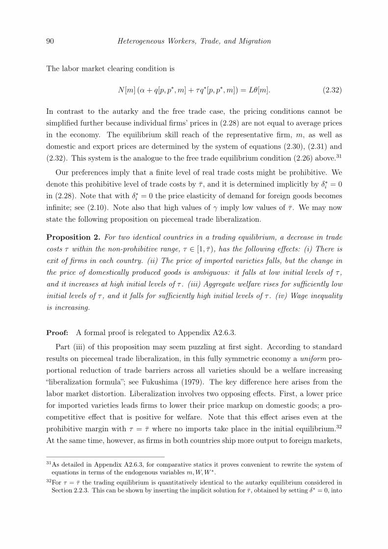
90 Heterogeneous Workers, Trade, and Migration
The labor market clearing condition is
N [m] (α + q[p, p∗,m] + τq∗[p, p∗,m]) = Lθ[m]. (2.32)
In contrast to the autarky and the free trade case, the pricing conditions cannot besimplified further because individual firms’ prices in (2.28) are not equal to average pricesin the economy. The equilibrium skill reach of the representative firm, m, as well asdomestic and export prices are determined by the system of equations (2.30), (2.31) and(2.32). This system is the analogue to the free trade equilibrium condition (2.26) above.31
Our preferences imply that a finite level of real trade costs might be prohibitive. Wedenote this prohibitive level of trade costs by τ , and it is determined implicitly by δ∗i = 0
in (2.28). Note that with δ∗i = 0 the price elasticity of demand for foreign goods becomesinfinite; see (2.10). Note also that high values of γ imply low values of τ . We may nowstate the following proposition on piecemeal trade liberalization.
Proposition 2. For two identical countries in a trading equilibrium, a decrease in tradecosts τ within the non-prohibitive range, τ ∈ [1, τ), has the following effects: (i) There isexit of firms in each country. (ii) The price of imported varieties falls, but the change inthe price of domestically produced goods is ambiguous: it falls at low initial levels of τ ,and it increases at high initial levels of τ . (iii) Aggregate welfare rises for sufficiently lowinitial levels of τ , and it falls for sufficiently high initial levels of τ . (iv) Wage inequalityis increasing.
Proof: A formal proof is relegated to Appendix A2.6.3.
Part (iii) of this proposition may seem puzzling at first sight. According to standardresults on piecemeal trade liberalization, in this fully symmetric economy a uniform pro-portional reduction of trade barriers across all varieties should be a welfare increasing“liberalization formula”; see Fukushima (1979). The key difference here arises from thelabor market distortion. Liberalization involves two opposing effects. First, a lower pricefor imported varieties leads firms to lower their price markup on domestic goods; a pro-competitive effect that is positive for welfare. Note that this effect arises even at theprohibitive margin with τ = τ where no imports take place in the initial equilibrium.32
At the same time, however, as firms in both countries ship more output to foreign markets,
31As detailed in Appendix A2.6.3, for comparative statics it proves convenient to rewrite the system ofequations in terms of the endogenous variables m,W,W ∗.
32For τ = τ the trading equilibrium is quantitatively identical to the autarky equilibrium considered inSection 2.2.3. This can be shown by inserting the implicit solution for τ , obtained by setting δ∗ = 0, into

Chapter 2 91
they use up more resources for transport, which bids up wage rates and causes firm exitsin both countries.33 Fewer domestic firms imply larger markups on the labor market aswell as a lower average quality of matches between firms and worker skills. The magnitudeof this effect clearly depends on the initial level of trade costs; it is strongest at τ = τ anddisappears for τ = 1. The proof in the Appendix demonstrates that for τ = τ initially,the adverse labor market effect of a marginal reduction of τ dominates, not just in termsof higher prices for domestic varieties, but also in terms of welfare so that liberalizationis welfare reducing. Since we can also demonstrate that free trade, τ = 1, is better thanautarky, τ = τ , there is a threshold value τ , with 1 < τ < τ , such that piecemeal liber-alization starting from τ < τ is unambiguously welfare increasing. Proposition 1 impliesthat τ > 1.
Invoking costless compensation, we use average income to evaluate aggregate welfareeffects in an economy where heterogeneous workers are affected differently. Using theindirect utility function we see that welfare is affected by changes in prices of domesticand imported goods as well as by the change in m, which affects both average income andthe number of available varieties. The change in welfare can be expressed as
V =
(∂ ln θ
∂ lnm− ∂ lnP
∂ lnm
)m−Nδp−Nδ∗p∗. (2.33)
The increase in m, induced by a decrease in trade costs, affects welfare negatively througha decrease in average income θm[m] < 0 and a decrease in the number of firms, whichimplies an increase in the ideal price index Pm[m] > 0. The effects of changes in pricesof domestic and imported goods are weighted by the respective expenditure shares. Fora high initial level of trade costs the expenditure share for imported goods is small, sothat consumers hardly benefit from the decrease in the price of imports, while being muchaffected by the change in the price of domestic goods, which is positive for a high initiallevel of trade costs. Hence, for a high initial level of τ the overall effect of a decrease in thetrade cost level on welfare is negative. In contrast, for a low initial value of trade costs, thenegative effect through a decrease in the number of firms becomes smaller, approachingzero as τ converges to one. Furthermore, the higher the expenditure share for importedgoods, the more consumers benefit from lower import prices, the more important therefore
the pricing condition (2.30). Yet, the disciplinary effect of a decrease in import prices works throughln p in equation (2.30), even if δ∗ = 0.
33This is the mechanism underlying the well-known home market effect for asymmetric countries, firstnoted by Krugman (1980). Of course, the home market effect as such does not arise here, since countriesare assumed symmetric.
92 Heterogeneous Workers, Trade, and Migration
also the competitive effect on domestic prices through the product market. Hence, wefind a U-shaped relationship between welfare and the level of trade costs.
2.4 Migration
So far, we have analyzed the effects of product market integration under the assumptionthat workers are immobile across countries. Intuitively, if we allow for migration, thensome workers in both countries will find their skills matching better with a firm in theforeign country. This constitutes an incentive for two-way migration. In this section, weshow that a “free trade cum migration” equilibrium delivers higher welfare than a “freetrade only” equilibrium. Furthermore, we show that under a slightly stronger assumptionabout the curvature of f [d], piecemeal integration of labor markets, unlike piecemeal tradeliberalization, is unambiguously welfare increasing. Our model highlights two welfareincreasing effects of migration: First, integration of labor markets reduces monopsonypower, as domestic firms now compete for workers not only with other domestic firms, butalso with foreign firms. Second, migration entails efficiency gains by improving the averagematching quality, as workers in both countries are now able to find better skill matchesfor employment. Even though the number of available varieties might fall, compared tothe free trade equilibrium, the efficiency gains and the pro-competitive gains on the labormarket are always dominating, leading to a positive welfare effect.
2.4.1 Modeling Migration
For simplicity, we consider the case of two symmetric countries, which implies the samenumber of firms in both countries, as well as equal prices and wages. This simplificationallows us to focus on the part of migration that is related to the idea of skill mismatch. Wedeliberately ignore differences in average wages or in the cost of living that would clearlyconstitute migration incentives as well.34 We model the cost of migration as reducing theproductivity of a worker to a fraction 1 − λ, if this worker moves to the other country.A domestic worker working for a domestic firm at distance d, delivering f [d] efficiencyunits, thus delivers only f [d](1 − λ) efficiency units when working for a foreign firm at
34Labor mobility and free entry imply that there is also the possibility of an agglomeration equilibrium,where all workers and firms work and produce in the same country. This is ruled out, if the trade costlevel is sufficiently low, compared to the cost of migration. Throughout this section, we assume freetrade, hence our results are not impaired by instability. In the case of zero cost of both trade andmigration, the equilibrium outcomes in the dispersed and the agglomeration equilibrium are the samein terms of prices and welfare.

Chapter 2 93
the same skill distance d.35 Symmetry of countries also means that the degree of skilldifferentiation among the labor force is the same.
We analyze international migration as an entry and pricing game with two stages andBertrand behavior analogous to sections 2.2 and 2.3 above, occurring simultaneously inboth countries, whereby each firm takes into account the possibility of hiring workers fromthe other country. Conditions similar to the ones discussed in Section 2.2.2 ensure exis-tence and uniqueness of the symmetric alternating location equilibrium for non-prohibitivemigration cost; see Appendix A2.7.1 for details. By alternating pattern, we mean any onefirm facing two neighboring firms from the other country.
2.4.2 Labor Supply with Integrated Labor Markets
We continue using 2m to denote the skill distance between two firms located in the samecountry. In the alternating equilibrium the firm’s direct competitor on the labor market,which is located in the foreign country, is then found at distance m in the skill space.36
The sorting cut-offs, i.e., the maximum distances of native workers dn and migrant workersdm from their firms, are derived as follows. For a domestic firm i, taking the foreign wagew∗ as given, the cut-off for native workers, dni = dni [wi, w
∗,m, λ], is determined by
wif [dni ] = w∗f [m− dni ](1− λ). (2.34)
Analogously, the cut-off for migrant workers, dmi = dmi [wi, w∗,m, λ], is determined by
wif [dmi ] = w∗f [m− dmi ]1
1− λ. (2.35)
As the level of migration costs falls, the cut-offs converge. At λ = 0 they coincide at m/2.
Under symmetry, the employment and migration pattern will be as follows: The do-mestic firm employs domestic workers with skill-types in the interval (s0−dn, s0 +dn), andforeign workers (migrants) located in the interval (s0−dm, s0 +dm), while the foreign firmlocated at s0+m will employ foreign workers located in the interval (s0+m−dn, s0+m+dn)
and domestic workers (migrants) with skill types in the interval (s0 +m−dm, s0 +m+dm).Notice that dn + dm = m.
35The proportionality assumption is convenient for modeling, yet it is not crucial. A general characteri-zation of the specifications generating the results derived in this section is found in Appendix A2.7.5.
36Note that without migration 2m measures the distance to the nearest competitor.

94 Heterogeneous Workers, Trade, and Migration
The supply of efficiency units as a function of the firm’s wage now emerges as
LES,M [wi, w∗,m, λ, L,H] =
L
H
dni [wi,w∗,m,λ]∫
0
f [d]dd+
dmi [wi,w∗,m,λ]∫
0
f [d](1− λ)dd
(2.36)
where dni [wi, w∗,m, λ] and dmi [wi, w
∗,m, λ] are given by (2.34), (2.35), respectively. Letdn = dn[m,λ] and dm = dm[m,λ] := m − dn[m,λ] denote the cut-offs in the symmetricequilibrium. These two variables measure the skill reach of a representative firm fordomestic and foreign workers, respectively. With λ > 0, we have dm < dn. As before,m may be interpreted as a mismatch indicator, but the average distance between workerskills and a firm’s ideal type across employment of domestic and foreign workers is nowequal to m/2, whereas without migration it was equal to m. In a symmetric equilibrium,average productivity then emerges as
θM [m,λ] :=1
m
(∫ dn
0
f [d]dd+
∫ dm
0
f [d](1− λ)dd). (2.37)
By complete analogy to (2.15), the perceived elasticity of effective labor supply, evaluatedat the symmetric equilibrium, can be derived as37
ηM [m,λ]∣∣wi=w∗
=2f [dn]2
f ′[dn] + (1− λ)f ′[m− dn]
−1∫ dn0f [d]dd+ (1− λ)
∫ dm0
f [d]dd. (2.38)
Note that the labor supply function is subject to the constraint dm[m,λ] ≥ 0, whichensures that both cut-offs lie in between the positions of the domestic and the foreignfirm. This condition is equivalent to the condition that the migration cost level λ is notprohibitive.38 As migration costs approach the prohibitive level, the supply of efficiencyunits of labor becomes equal to the supply under autarky. This is readily verified byinserting dn = m and dm = 0 into (2.36).
Interestingly, even if the level of migration costs is prohibitive, firm behavior is influ-enced by the mere potential of migration through the perceived elasticity of labor supply.39
The possibility of attracting migrants by setting higher wages and thus increasing the sup-ply of efficiency units implies that firms perceive a higher elasticity of supply, even if they
37For details of the derivation see Appendix A2.7.238Otherwise, if migration costs are too large relative to firm size, firms cannot attract any migrants inthe first place and the supply curve looks different since they then compete again only with firms fromthe same country.
39We thank Vitor Trindade for pointing this out to us.

Chapter 2 95
do not employ any migrant in equilibrium. Let λ denote the prohibitive level of migrationcosts, determined by setting dm[m,λ] = 0. The perceived wage elasticity of labor supplyevaluated at λ is given by
ηM [m, λ] =2f [m]2
f ′[m] + (1− λ)f ′[0]
−1
F [m]. (2.39)
Note that concavity of f [d] is sufficient to ensure that ηM [m, λ] is larger than the elas-ticity of supply under autarky as given in (2.15). It is important to note at this point,that with prohibitive λ, the symmetric alternating location pattern does not constitutean equilibrium as defined in (2.14). The reason is precisely that in this situation, labormarket competition is greater than in autarkic labor markets, while labor supply is thesame. Firms can and will avoid this situation, for example, by simultaneously decreasingthe distance to one of their foreign neighbors, leading to a de-facto autarkic labor marketequilibrium. Nevertheless, the second-stage pricing equilibrium evaluated at the symmet-ric alternating location pattern and prohibitive cost of migration proves very helpful asa reference case for the equilibrium outcomes of the cases of non-prohibitive migrationcost, for which the symmetric alternating location pattern does constitute the uniqueequilibrium of the two-stage game.
We show in Appendix A2.7.2 that ηM [m,λ] increases as λ falls, provided that f ′′′[d]
is not too large. In what follows, we assume that this condition holds.40 By analogy to(2.17), we now use ψM [m,λ] :=
(ηM [m,λ] + 1
)/ηM [m,λ] to denote the wage distortion
under migration. For a given level ofm, the magnitude of this distortion is unambiguouslylower with migration and λ ∈ [0, λ] than without.
In addition to the wage distortion, migration also affects the average quality of skillmatches between workers and firms. It is obvious that for prohibitively high migrationcosts, λ = λ, the average matching quality, as given in equation (2.37), is the same asunder autarky, given in (2.18): θM [m, λ] = θ[m]. Moreover, as we prove in the appendix,θMλ < 0. In other words, the matching quality unambiguously increases as λ falls, reachingθM [m, 0] = θ[m/2] for frictionless migration where λ = 0. It is instructive to see how
40The reasoning behind this condition is as follows: A higher λ leads firms to increase the share ofmigrants employed by shifting dn outwards and dm inwards. If the curvature of f [d] falls (in absoluteterms) as the cut-offs move to the right, an increase in λ helps firms to avoid competition by employingmore native workers in the range where the curvature of f [d] is lower and fewer migrants in the rangewhere the curvature of f [d] is strong. We rule this out by assuming that the curvature does not decreasetoo much (in absolute terms) as the cut-off moves to the right.

96 Heterogeneous Workers, Trade, and Migration
effective labor supply to a representative firm is affected by the cost of migration. Underfrictionless migration, λ = 0, labor supply (2.36) emerges as
LES,M = 2L
H
∫ m2
0
f [d]dd =2L
NMθM [m, 0] =
L
Nθ [m/2] . (2.40)
Note that NM = 2Hm
= 2N , where N is the number of firms in each country. Comparingthis to the autarky case, both the number of firms and workers are doubled. However,we know from above that for λ < λ we have θM > θ. Hence, with migration firms facea larger supply of efficiency units of labor than under autarky. The reason is that, whileemploying the same number of workers as under autarky, each firm now finds workers withskills closer to its optimal type. Importantly, all of this is conditional upon a given levelof m, which is determined by the firm entry condition. As we shall see below, equilibriumadjustment of the number of firms after opening up to migration, driven by a lower wagemarkup, might bring about firm exit which has a countervailing, negative effect on averageproductivity.
2.4.3 The “Trade cum Migration” Equilibrium
We complete the description of a “trade cum migration” equilibrium for non-prohibitivemigration costs by a zero profit condition that determines the number of firms or, equiv-alently, the distance between a neighboring domestic and foreign firm on the skill circle,which is now equal to m. We look at the case of free trade. As in (2.26), we formulatethis condition as stating that the double markup is equal to the inverse of the degree ofeconomies of scale:
gM [m,λ] = ρT [m]ψM [m,λ]. (2.41)
In this equation, ρT [m] denotes the free trade price markup over perceived marginalcost obtaining in a free trade equilibrium without migration. Under free trade, thismarkup simplifies to 1 + 1/(γNM), where NM is the number of firms world-wide; seeequation (2.24). Unlike the wage markup, the price markup is not affected by allowingfor migration. The term ψM [m,λ] denotes the wage markup in a migration equilibrium, asintroduced above. The term gM [m,λ] on the left measures the degree of scale economies,taking into account the labor market clearing condition, which now reads as α + q =

Chapter 2 97
(m/H)LθM [m,λ], as well as goods market clearing, which requires q = LθM [m,λ]/(pN).This measure thus reads as
gM [m,λ] :=LθM [m,λ]
LθM [m,λ]− αH/m. (2.42)
In order to understand the effects of labor market integration, we now proceed in twosteps. We first look at a situation where migration is allowed in principle, but wherethe costs of migration are prohibitively large, λ = λ, and compare this case with theequilibrium outcome under national labor markets. Importantly, as we have discussedabove, the case of prohibitive migration cost we are referring to in this section describesthe second-stage pricing equilibrium for a symmetric alternating location pattern, butdoes not constitute a subgame-perfect equilibrium as defined in (2.14). It serves only asa reference case for the second step, where we look at the effects of successively loweringthe costs of migration, starting from non-prohibitive levels of λ, for which the symmetricalternating location pattern does constitute a subgame-perfect equilibrium.
Proposition 3. Compared to a free trade equilibrium with national labor markets, welfareis unambigously higher in the second-stage “trade cum migration” equilibrium with twosymmetric countries, symmetric alternating firm locations, and a prohibitively high levelof the cost of migration. The number of firms in each country is unambigously smaller inboth countries.
Proof: The analytical details of the proof are relegated to Appendix A2.7.3.
A key point to understand this proposition is that the excess entry property of theautarky equilibrium demonstrated in Section 2.2.4 is inherited by the second-stage zero-profit equilibrium with symmetric alternating location patterns for any λ ∈ [0, λ]. Whilethe productivity distortion is not affected as long as no one migrates, the wage markupis affected because firms perceive a larger elasticity of labor supply. By lowering thewage markup, opening up labor markets to migration implies that the number of firms inthe zero-profit equilibrium is smaller, even if the cost of migration is prohibitively high.And given that the free trade equilibrium involves excessive firm entry, this entails apositive welfare effect. With a lower wage markup distortion relative to the productivitydistortion, the allocation is now closer to the social optimum.
Proposition 4. In a “trade cum migration” equilibrium with two symmetric countries,piecemeal integration of labor markets through a marginal reduction in the cost of migrationhas an ambiguous effect on the number of firms. However, it unambiguously leads to

98 Heterogeneous Workers, Trade, and Migration
lower prices and an increase in welfare in both countries, irrespective of the initial levelof migration costs λ ∈ [0, λ].
Proof: The analytical details of the proof are relegated to Appendix A2.7.4.
The intuition for this proposition is best grasped from Figure 2.3, which depicts theschedules gM [m,λ] and ρT [m]ψM [m,λ], identifying the equilibrium value of m at the in-tersection, in line with the zero profit equilibrium condition (2.42). The vertical axis ofFigure 2.3 may be interpreted as measuring goods prices. Remember that gM [m,λ] mea-sures the inverse degree of scale economies, which is equivalent to the markup requiredfor zero profits. An increase in m makes firms larger, but it also lowers the productiv-ity of the average worker. The appendix shows that the size effect always dominates,whence the gM -line is downward-sloping. The ρT [m]ψM [m,λ]-line depicts the doublemarkup, reflecting monopoly power on the goods market and monopsony power on thelabor market, respectively. This line is unambiguously upward-sloping, as a lower num-ber of firms (higher m) reduces both the perceived price elasticity of goods demand aswell the perceived labor supply elasticity with respect to the wage rate. We know fromproposition 3 above that the intersection point for λ = λ involves a lower value of mthan in the free trade equilibrium with national labor markets, which is determined byg[m] = ρT [m]ψ[m].41
Now consider a reduction in λ from λ to λ1 ∈ [0, λ). For a notionally unchanged valueof m, this improves the productivity of the average worker through a higher inframarginalsurplus on migrant labor as well as through a resorting of workers from native employmentinto migration.42 This means that the gM -line is shifted down by a reduction in λ. Asregards the markup schedule ρT [m]ψM [m,λ], we have shown above that the perceivedelasticity of labor supply increases with a lower cost of migration, meaning that for anotionally unchanged m firms charge a lower wage markup ψM [m,λ]. Thus, the markupschedule shifts down as well, rendering an ambiguous effect on m. In the figure, thecase gM [m,λ1] (gM [m,λ1]′) depicts a relatively weak (strong) shift in the gM -line, leadingto an increase (a decrease) in m. The ambiguity in the adjustment of m implies thatwage inequality under migration can generally be lower or higher than in the free tradeequilibrium. However, the equilibrium unambiguously moves down on the vertical axis,which implies lower goods prices.
41Moving from an equilibrium with national labor markets to a “trade cum migration” equilibrium withλ = λ leaves g unaffected, g[m] = gM [m, λ], while reducing the wage markup, ψ[m] > ψM [m, λ].
42Note that for a constantm the average skill distance between workers and their firm’s ideal type remainsconstant, equal to m/2. The productivity gain arises from savings in migration costs.

Chapter 2 99
m
gM [m, λ] = g [m]
gM [m, λ1]
gM [m, λ1]′
ρT [m]ψ[m]
ρT [m]ψM [m, λ]
ρT [m]ψM [m, λ1]
gM [m, λ]
mAm′
λ1mλ1
mλ
Figure 2.3: Comparative statics of the skill reach m
The welfare effect is determined by the change in real income and the number ofvarieties. Real income is given by θM [m,λ]
/p[m], where average “nominal” income is
measured by θM [m,λ], the productivity of the average worker. Invoking the indirectutility function, the welfare effect of our scenario may be described as
V =∂ ln
[θM/p
]∂λ
· dλ+∂ ln
[θM/p
]∂m
· dm− 1
4γH· dm (2.43)
The first term describes the direct effect of lower migration costs, dλ < 0, on real in-come. From the above we know that this term is unambiguously positive. The remainingterms involving dm are ambiguous in their entirety, because dm as caused by dλ < 0 isambiguous. However, we know from the above discussion of the distortions present inthis economy that the autarky equilibrium involves excess firm entry, and from the proofof proposition 3 we know that any second-stage “trade cum migration” equilibrium withsymmetric alternating firm locations inherits this excess entry property. Therefore, thepositive real income effect of firm exit in the second term must dominate the negativevariety effect in the third term. In other words, if the equilibrium adjustment depictedin Figure 2.3 leads to dm > 0, then the overall effect of dλ < 0 on welfare is positive.If dm < 0, then the welfare effect is less straightforward. While the final term of thisexpression is then unambiguously positive, the first two terms seem ambiguous. However,we show in the appendix that the first two terms of (2.43) are unambiguously positive
100 Heterogeneous Workers, Trade, and Migration
for any initial λ ∈ [0, λ], if we insert dm = (∂m/∂λ) · dλ. Referring to our discussionsubsequent to propositions 1 and 2, we repeat that individual households are affecteddifferently, due to skill heterogeneity. Speaking of an aggregate welfare effect implies theexistence of a costless (lump-sum) redistribution mechanism.
2.5 Conclusion
In this paper, we propose an important qualification to the common narrative of of variety-based gains from trade. Traditional models of monopolistic competition stress the impor-tance of a large resource base for a large degree of product differentiation, if productionis subject to a non-convex technology. By opening up to trade, even small countries mayenjoy the benefits of a large resource base. Domestic firms may be driven out of themarket, but this has no adverse effect. If anything, it increases the average productivitylevel through a positive selection effect.
This view neglects an important fact of modern manufacturing: Product differentiationrelies on the availability of differentiated inputs, including non-traded inputs like labor.If producing a specific variety of a good requires a specific bundle of skills, then theskill-diversity of the labor force, rather than its size, determines the degree of productdifferentiation supplied by the market. In this paper, we have shown that trade is asomewhat less benign force in an environment where product differentiation is based onworker heterogeneity than portrayed in conventional models of monopolistic competition.In particular, trade-induced firm exit worsens the average quality of matches betweenthe type of skills that workers bring to their firms and the specific skill requirementsof the goods produced by these firms. In addition, product differentiation implies thatfirms have monopsony power in the labor market, whence trade-induced exit of firmsincreases the resulting distortion between the marginal productivity of labor and the wagerate. This works against the conventional pro-competitive effect of trade on the goodsmarkets where trade lowers the markup between marginal cost and prices. Labor marketintegration gives rise to a migration incentive, whereby firms engage in cross-border hiringeven under complete symmetry between countries. Migration essentially has effects thatare opposite to those of trade.
We have developed a model which allows us to rigorously pin down these effects andto weigh them against the effects familiar from conventional models of monopolistic com-petition. In our model product differentiation is rooted in preferences represented by atranslog expenditure function. When entering the market, firms decide upon which typeof good to produce, based on a circular representation of skill heterogeneity among the

Chapter 2 101
work force, where each worker has the potential to serve as an “ideal” worker for a spe-cific type of good. A non-convex technology implies a finite number of firms. A worker’ssupply of efficiency units is inversely related to the distance between her skill-positionon the circle and the ideal skill position of the firm she works for. Having positionedthemselves on the circle upon entry, firms engage in Bertrand competition on goods andlabor markets, setting a double markup.
Using this model, we have explored both trade and migration scenarios. Comparing freetrade with autarky in a symmetric many-country-world, we find that the variety and pro-competitive effects on goods markets unambiguously dominate the adverse effects froma lower average quality of matches between firms and workers and from higher markupson the labor market. Looking at piecemeal trade liberalization between two symmetriccountries, we find an ambiguity: If liberalization takes place from a high initial level oftrade costs, then it causes a lowering of aggregate welfare, whereas it increases aggregatewelfare, if the initial level of trade costs is already below a certain threshold.
Starting from a free trade equilibrium in a symmetric two-country-world, integratinglabor markets leads to two-way migration. Firms and workers in both countries face anincentive for cross-border hiring, even though the initial equilibrium features internationalwage equalization. Thus, our view of product differentiation based on worker heterogene-ity generates a novel force of migration, contributing to an improved understanding oftwo-way migration, which looms large in the data but has so far lacked convincing ex-planation in standard models of migration. Interestingly, potential migration exerts apositive welfare effect on both countries, even if migration costs are prohibitively large.Contrary to piecemeal trade liberalization, a piecemeal reduction in the cost of migra-tion is unambiguously welfare increasing. The reason is that it improves the quality ofmatches while at the same time lowering firms’ monopsony power on labor markets. Fromthe simple fact that trade and migration have opposite effects it also follows that tradeand migration are complements, rather than substitutes. The model clearly advocatesopening up labor markets simultaneously with trade liberalization.

Appendix A.2
A2.1 Expenditure Share and Markup
Starting out from Equation (2.6), we obtain
δi =1
N+ γln p− γ ln
δiY
qi
by inserting pi = δiYqi. This can be rewritten as
δiγ
+ lnδiγ
=1
γN+ ln p− ln
Y
qi− ln γ
and applying the Lambert function W [z] which is defined as the solution to xex = z or,equivalently, to lnx+ x = ln z, yields δi = δ[qi, ln p,N, Y ] as defined in Equation (2.8).
Similar logic can be applied to obtain an explicit solution for the optimal price asdetermined by (2.11). Defining perceived marginal cost as wi := [(ηi + 1)/ ηi]wiβ andobserving (2.6) and (2.10) the first-order condition (2.11) can be written as
piwi
+ ln pi = 1 +1
γN+ ln p. (A2.1)
The left-hand side is an implicit function of the profit maximizing price pi. Rewriting(A2.1) as
piwi
+ ln pi − ln wi = 1 +1
γN+ ln p− ln wi (A2.2)
and applying the Lambert function to the left-hand side, we obtain the following explicitsolution for pi
pi =W[w−1i exp
{1 +
1
γN+ ln p
}]wi. (A2.3)
which implies that the price markup obeys
εiεi − 1
=W[
ηiwi(ηi + 1)
exp
{1 +
1
γN+ ln p
}].
A2.2 Existence and Uniqueness of the Pricing Equilibrium (Lemma 1)
We invoke the Index Theory approach outlined in (c.p. Vives, 2001, p. 48) to proof thatunder certain restrictions on the parameter space, there is a unique solution to secondstage game. It follows, that π∗[m, N ] is unique. The Index Theorem approach is based on

Chapter 2 103
the Poincaré-Hopf Index Theorem, which implies that a solution to a system of reactionfunctions is unique if
i). payoff functions are quasiconcave in firms’ own strategies,
ii). the strategy space is convex and compact and all equilibria are interior,
iii). the Hessian is negative definite at the equilibrium point.
The proof proceeds as follows: We show that condition i) holds if the elasticity of marginallabor supply is not too large and condition ii) holds if marginal revenue is positive foroutput levels arbitrarily close to zero. Then, we show that condition iii) is always fulfilledin a transformed game where firms’ strategies are log wages. Since conditions i) and ii)also hold in the transformed game, the Index Theorem implies that the transformed gamehas a unique solution. Since lnw is a positive monotone transformation of w for w > 0,this, in turn, implies uniqueness of the solution to the original game.
i) Quasi-concavity of the profit function. In the second stage, firms take the distancepattern mi, aggregate income Y and the average log price ln p as given and determinetheir optimal wage as best response against other firms’ wage choices w−i by maximizingprofits as in (2.9). The set of permissible strategies is bounded from below by wαi :=
L−1[α,w−i,mi] > 0, which denotes the wage-level where the second constraint in (2.9)binds.43 Moreover, firms never set wages above the choke price divided by the marginallabor requirement β, where
pchoke := pchoke[N ] = limqi→0
mri = exp
[1
γN+ ln p
]with
mri := mr[qi, N, Y, ln p] =∂ri∂qi
=ri
(W qi + 1)qi
> 0
that is, the price at which demand approaches zero. Hence, there is a common upper
bound on firms’ strategies w =exp[ 1
γN+ln p]
βand so firm i’s strategy set is Si = [wαi, w].44
In the above and the subsequent equations, we use W qi := W
[exp
{1γN
+ ln p}
qiγY
]to
denote the markup. Moreover, we henceforth denote with Li := LS[wi,w−i,mi] firm i’slabor supply.
43wαi approaches zero as all firms lower their wages towards zero. We assume that wαi is positive becauseotherwise lnw (which we will be working with below) is not defined. This assumption has no bearingon the equilibrium outcomes. Moreover, excluding the possibility of zero wages can be justified byassuming that at a zero wage, workers prefer not to work and hence, firms need to pay at least thereservation wage.
44Note that pchoke is the upper bound on marginal revenue and wβ is the lower bound of firms’ marginalcost. Hence, wages above pchoke/β entail negative marginal profits independent of other firms’ choicesand are thus strictly dominated.

104 Heterogeneous Workers, Trade, and Migration
A sufficient condition for π[wi,w−i,mi, N ] to be quasiconcave in the firm’s own strat-egy is that ∂2πi
∂w2i< 0 whenever ∂πi
∂wi≥ 0. Marginal profits are given by
∂πi∂wi
=
(mriβ− wi
)∂Li∂wi− Li if
∂Li∂wi∃,
where
∂Li∂wi
=L
2H
∑c=`,r
f [di,c]ddi,cdwi
> 0 withddi,cdwi
=f [di,c]
−wif ′[di,c]− wcf ′[2mi,c − di,c]> 0.
(A2.4)
Marginal profits change in the firm’s wage according to
∂2πi∂w2
i
=∂mri∂qi
1
β2
(∂Li∂wi
)2
− 2∂Li∂wi
+
(mri[qi]
β− wi
)∂2Li∂w2
i
if∂Li∂wi∃, (A2.5)
where
∂2Li∂w2
i
=L
2H
(∑c=`,r
3f ′[di,c]
(ddi,cdwi
)2
+ (wif′′[di,c]− wcf ′′[2mi,c − di,c])
(ddi,cdwi
)3)
Q 0
(A2.6)∂mri∂qi
=− mriqi
W qi (W q
i + 2)
(W qi + 1)2
(A2.7)
Rewriting Equation (A2.5), we obtain
α + βqiβqi
· |εmr,i| ≥ηmls,iηi
(A2.8)
as a sufficient condition for quasiconcavity, where
εmr,i =∂mri∂qi
qimri
= −Wqi (W q
i + 2)
(W qi + 1)2
≤ 0
ηmls,i =∂2Li∂w2
i
wi
/∂Li∂wi
≶ 0.
With concave revenue in qi, quasiconcavity of profits clearly obtains while the laborsupply function is concave, since this implies that revenue is also concave in wi and thatthe cost function wiLi is convex in wi. Concavity of the labor supply function impliesthat the wage elasticity of marginal labor supply ηmls is negative and, therefore, condition(A2.8) clearly holds. More generally, condition (A2.8) holds if ηmls is not too large relativeto η. Moreover, condition (A2.8) holds irrespective of the curvature of the labor supply

Chapter 2 105
function if LiLi−α = α+βq
βq, the inverse degree of economies of scale, is large. This is always
the case for low levels of the marginal cost β. To again more intuition about the role ofβ, note that 1/β is the derivative of qi with respect to Li, hence for any given level, slope,and curvature of Li, β determines the relative weight of the curvature of revenue on thecurvature of the profit function. Hence, whenever ∂Li
∂wi∃, quasiconcavity obtains if β is
sufficiently small or if the labor supply function is concave.
Whenever firm i chooses a wage so that its neighbor i + j is just overbid and i startscompeting with the next relevant competitor i + j′, j′ > j, the labor supply functionand thus the profit function exhibits a kink and ∂Li
∂wi6 ∃. However, we can show that the
labor supply function is always flatter after the kink and hence, the kinks do not impairthe concavity of the profit function. Let wi,c := wi,c[w−i,mi] denote the wage where therelevant competitor on side c = `, r is just overbid. Then, (A2.4) implies that
limwi→w−i,c
∂Lci∂wi
=L
2H
f [di,c[wi,c]]2
−wi,cf ′[di,c[wi,c]]− wi+jf ′[2mi,i+j − di,c[wi,c]]and (A2.9)
limwi→w+
i,c
∂Lci∂wi
=L
2H
f [di,c[wi,c]]2
−wif ′[di,c[wi,c]]− wi+j′f ′[2mi,i+j′ − di,c[wi,c]]. (A2.10)
If i+ j was overbid by i+ j′ at its own location, limwi→w−i,c∂Lci∂wi≥ limwi→w+
i,c
∂Lci∂wi
followsfrom −f ′[2mi,i+j′ − di,c[wi,c]] > −f ′[2mi,i+j − di,c[wi,c]] > 0 and wi+j′ > wi+j.
If i+ j was overbid by i at its own location, limwi→w−i,c∂Lci∂wi≥ limwi→w+
i,c
∂Lci∂wi
follows from2mi,i+j′ − di,c[wi,c] < 0 and −f ′[2mi,i+j′ − di,c[wi,c]] > 0 > −f ′[2mi,i+j − di,c[wi,c]] > 0.
A similar argument applies to the slope of the labor supply on firm i’s other side ifit also exhibits a kink at wi,c. Otherwise, the derivative of the labor supply functionon that side exists. It follows that limwi→w−i,c
∂πi∂wi≥ limwi→w+
i,c
∂πi∂wi
if(mriβ− wi
)> 0. If(
mriβ− wi
)< 0, then limwi→w−i,c
∂πi∂wi
, limwi→w+∂πi∂wi
< 0.
This proves that under the conditions specified above, profits are globally quasiconcave.
ii) The strategy space is convex and compact, and all solutions are interior if thedegree of substitutabilty of products γ is sufficiently small. Firm i’s strategy spaceis given by the interval Si = [wα,i, w] and hence it is convex, closed and bounded. Interiorsolutions require that the slopes of the profit functions at the boundaries of the strategyspace point inwards. At the lower bound, this condition holds if marginal revenue at wi,that is, at qi = 0, is sufficiently large. Sufficiently small values of γ for any fixed number offirms, a given average price, fixed and variable cost, and labor market conditions w−i,mi,ensure that ∂πi
∂wi
∣∣∣wi=wi
=(pchokeβ− wi
)∂Li∂wi
∣∣∣wi=wi
− α > 0. Li[w,w−i,mi] > α if w > wα,i
implies ∂πi∂wi
∣∣∣wi=wi
< 0.

106 Heterogeneous Workers, Trade, and Migration
iii) The Hessian of the log-transformed game is negative definite at the equilibriumpoint. We prove negative definiteness of the Hessian by showing that the game in trans-formed strategies lnwi ∈ Si, where Si = [lnwα,i, ln w], exhibits diagonal dominance at theequilibrium point where
∂πi∂ lnwi
= 0 ∀i
Diagonal dominance at the equilibrium point requires that∣∣∣∣ ∂2πi∂ lnw2
i
∣∣∣∣− N∑j 6=i
∣∣∣∣ ∂2πi∂ lnwi∂ lnwj
∣∣∣∣ > 0, (A2.11)
where
∂2πi∂ lnw2
i
= wi∂πi∂wi
+ w2i
∂2πi∂w2
i
= w2i
∂2πi∂w2
i
sincewi∂πi∂wi
= 0
∂2πi∂ lnwi lnwj
=
{wiwj
∂2πi∂wiwj
for j = `, r0 for j 6= i, `, r
In an interior equilibrium no firm is overbid. This implies that around the equilibriumpoint the labor supply function is smooth and we do not need to worry about the kinks.Moreover, it implies that firm i’s relevant competitors are its immediate neighbors, thatis, ` = i− 1 and r = i+ 1.
Firm i’s marginal profits change in its neighbors’ log wages according to
∂2πi∂wi∂wc
wiwc =∂mri∂qi
1
β2
∂Li∂wi
∂Li∂wc
wiwc −∂Li∂wc
wiwc +
(mriβ− wi
)∂2Li∂wi∂wc
wiwc Q 0
(A2.12)
where
∂Li∂wc
wc =L
2Hf [di,c]
ddi,cdwc
wc < 0 sinceddi,cdwc
=f [2m− di,c]
wif ′[di,c] + wcf ′[2mi,c − di,c]< 0
(A2.13)∂2Li∂wi∂wc
wiwc =L
2H
(2f ′[di,c]
ddi,cdwi
widdi,cdwc
wc + f ′[2mi,c − di,c]ddi,cdwi
widdi,cdwi
wc
+ (wif′′[di,c]− wcf ′′[2mi,c − di,c])
ddi,cdwi
ddi,cdwi
widdi,cdwc
wc
)

Chapter 2 107
=L
2H
(−2f ′[di,c]
(ddi,cdwi
wi
)2
+ f ′[2mi,c − di,c]ddi,cdwi
widdi,cdwi
wc
− (wif′′[di,c]− wcf ′′[2mi,c − di,c])
ddi,cdwi
(ddi,cdwi
wi
)2)
Q 0. (A2.14)
The second step follows from ddi,cdwc
wc =ddi,cdwi
wi. Since the first two terms in Equation(A2.14) are always positive, it holds that∣∣∣∣ ∂2πi
∂wi∂wcwiwc
∣∣∣∣ ≤ ∂mri∂qi
1
β2
∂Li∂wi
∂Li∂wc
wiwc −∂Li∂wc
wiwc +
∣∣∣∣(mriβ − wi)
∂2Li∂wi∂wc
wiwc
∣∣∣∣ .Provided that condition i) holds, diagonal dominance as defined in Equation (A2.11) atthe equilibrium point obtains if
−∂mri∂qi
1
β2
(∂Li∂wi
wi
)2
+ 2∂Li∂wi
w2i −
(mriβ− wi
)∂2Li∂w2
i
w2i
≥∑c=`,r
(∂mri∂qi
1
β2
∂Li∂wi
∂Li∂wc
wiwc −∂Li∂wc
wiwc +
(mriβ− wi
)∂2Li∂wi∂wc
wiwc
)
⇔ −∂mri∂qi
1
β2
(∂Li∂wi
wi
)(∂Li∂wi
wi +∑c=`,r
∂Li∂wc
wc
)+∂Li∂wi
w2i + wi
(∂Li∂wi
wi +∑c=`,r
∂Li∂wc
wc
)
−(mriβ− wi
)(∂2Li∂w2
i
w2i −
∑c=`,r
∂2Li∂wi∂wc
wiwc
)≥ 0
⇔ mriβ
∂Li∂wi
wi ≥ 0
The last step follows from
∂Li∂wi
wi = −∑c=`,r
∂Li∂wc
wc and∂2Li∂w2
i
w2i −
∑c=`,r
∂2Li∂wi∂wc
wiwc = −∂Li∂wi
wi. (A2.15)
This proves that the game in log transformed strategies exhibits diagonal dominance atthe equilibrium point.
Since conditions i) and ii) clearly also hold for the transformed game, there exists aunique solution to this game. Since lnw is a monotone transformation of w for w > 0,uniqueness in the transformed game implies uniqueness of equilibrium in the originalgame. This completes the proof.

108 Heterogeneous Workers, Trade, and Migration
A2.3 Proof of Existence and Uniqueness of the Entry Equilibrium (Lemma 2)
We first prove that under condition ii) of Lemma 2 there is a unique number of firmsN sym ≥ 1 corresponding to a (symmetric) second stage equilibrium with π∗[msym, N
sym] =
0. Moreover, we show that π∗[msym, N ] = 0 is decreasing in N.
Existence and uniqueness of the second-stage zero-profit equilibrium for symmetricdistance patterns. As described in Section 2.2.3, for symmetric distance patterns asecond-stage zero-profit equilbrium is given by a root of the function
G[m] := π∗[msym, N ] = βρ[m]ψ[m]− βg[m] (A2.16)
where g[m] > 1 is the inverse of an aggregate version of the familiar measure of the degreeof scale economies, i.e., the ratio of average to marginal cost. We expect this to be fallingin m: The larger firm size m, and the smaller the number of firms, the closer average costto marginal cost. In turn, ρ[m] := 1 + 1
γN [m]and ψ[m] := η[m]+1
η[m]are the two markups
on the goods and the labor market, respectively. Given that a symmetric equilibriumhas N = H/m, we have ρm = 1/(γH) > 0. As shown in Section 2.2.3, ηm < 0, whencewe have ψm = −ηm/η[m]2 > 0. As expected from intuition, both markups are falling inthe number of firms and thus rising in the half-distance between two neighboring firms,m. Note that G[m] > 0 implies positive profits, while G[m] < 0 implies that firms makelosses.
The following conditions are sufficient for a symmetric zero-profit equilibrium to existand to be unique: a) G[H] > 0, b) G[m] is continuous and Gm > 0 in the interval (m,H],where m is defined by L
N [m]θ[m] = α.
Condition a) requires that a single firm in the market makes at least zero profits, thatis,
Lθ[H]
Lθ[H]− α≤(
1 +1
γ
)ψ[H]. (A2.17)
Observing that ψ[m] increases inm, we can set ψ[H] on the right-hand side to its minimumlevel of unity to obtain
α
Lβ(1 + γ) ≤ F [H]
H(A2.18)
which is a sufficient condition for (A2.17). It shows, that given α, β, L and H, the degreeof substitutability of goods in the utility function γ, that governs the price elasticity ofdemand, must not be too large. Relating back to (A2.17) in its original form, these

Chapter 2 109
restrictions imply that the price markup over marginal cost that a single firm can chooseexceeds its average cost.45
Condition b) requires that firm entry, which is associated with a decrease in the skill-reach m, lowers profits in the relevant range where firms produce positive output, that is,for m ∈ (m,H]. Since we know from above that ρm > 0 as well as ψm > 0, condition b)is satisfied if gm < 0. It is straightforward to show that
gm[m] =LHf [m]
mLHθ[m]− α
(1−
mLHθ[m]
mLHθ[m]− α
)< 0 for m ∈ (m,H]. (A2.19)
Hence, there exists a unique N sym ≥ 1 satisfying G[m] = π∗[msym, Nsym] = 0. Condi-tion b) and m = 2H
Nimply ∂π∗[msym,N ]
∂N< 0.
Existence and uniqueness of the symmetric sub-game perfect equilibrium With firmentry determined by (2.13) and consistent beliefs as described in Section (2.2.2), existenceofN sym satisfying π∗[msym, N
sym] = 0 implies that no (symmetric or asymmetric) distancepattern involving a number of firms smaller N sym can be an equilibrium according to(2.14).
To prove that msym|N sym is the unique equilibrium, it remains to show that there isno other distance pattern with N ≥ N sym that is consistent with (2.13) and (2.14). Wedo so by showing that every asymmetric distance pattern with N ≥ N sym firms and everysymmetric distance pattern with N > N sym firms implies negative profits for at least onefirm, which implies ν(N) = 0 for all N > N sym. The result for symmetric distance vectorsfollows readily from ∂π∗[msym,N ]
∂N< 0. The proof for asymmetric location patterns is slightly
more involved and requires restrictions on the parameter space. It runs along the followingline of argument. We conjecture that the symmetric zero profit solution characterized byπ∗[msym, N
sym] = 0 is an equilibrium and then consider any possible change towards anasymmetric location pattern featuring the same or a larger number of firms. Since thesymmetric location pattern maximizes labor supply per firm, such a change must bringabout a decrease in q for at least one firm. Let j be the firm that produces the smallestquantity in any arbitrarily chosen asymmetric location pattern with N sym firms. Then,we can show that if the marginal cost β are sufficiently small, firm j’s profits must benegative in the asymmetric pattern. Hence, no asymmetric location pattern can be anequilibrium consistent with optimal entry choices of entrants and non-entrants.
45This condition is well known from the standard New Trade Theory model with homogeneous workers(cp. Equation (10) in Krugman, 1980).

110 Heterogeneous Workers, Trade, and Migration
From the point of view of any firm i, a zero-profit equilibrium is characterized by
ρ[N, qi, q−i] · ψ[mi, N ] = g[qi] where g[qi] =Li
Li − α=α + βqiβqi
, ∀
which states that the product of markups equals the inverse of the degree of economies ofscale (cp. Equation (2.22)).46 Note that qi = Li[mi,N ]−α
βis also a function of the location
pattern and so are ρ[N, qi, q−i] and g[qi].47 However, it will prove important that g[·] andρ[·] depend on mi only through output quantities, since we may therefore pin down thechanges in g[·] and ρ[·] for firm j for an arbitrary change in the location pattern, since,by definifion, qj decreases whenever we move away from symmetry.
From the point of view of any firm, the change towards an asymmetric location patterncan be described in terms of changes in potentially all elements of the distance vectormi. Its profits are affected by corresponding changes in the markups and the degree ofeconomies of scale. In the new location pattern, firm i’s profits will be negative if andonly if the total markup (ρiψi) increases by less (falls by more) than the inverse of thedegree of economies of scale, gi. That is, a sufficient condition for π∗[mi, N
sym] < 0 forall mi 6= msym is that
d(ρi · ψi) = ρidψi + ψidρi < dgi, where (A2.20)
dgi =∂g[qi]
∂qi
∂qi∂Li
dLi = − α
(βqi)2dLi with dLi =
N∑k
∂Li∂mk,k+1
dmk,k+1
(A2.21)
dρi =N∑k
∂ρi∂qk
∂qk∂Lk
dLk (A2.22)
dψi =1
ηi
dLiLi− 1
ηi
N∑k
∂2Li∂wi∂mk,k+1
∂Li∂wi
dmk,k+1 (A2.23)
Note that Li depends on the distances between all firms and not just firm i’s neighbors,because it is a function of firm i’s own and its neighbors’ equilibrium wages in the secondstage, which jointly solve all firms’ first-order conditions and therefore depend on thecomplete distance vector.
46Using the first-order condition (2.11), we can write optimum profits π∗[mi, N ] of any firm as
π∗i = w∗iLi
(ψiρi
Li − αLi
− 1
).
Then, for w∗i , Li > 0, π∗i = 0 iff ρiψi = gi.47The dependence of ρi on q−i derives from the dependence of ρi on total expenditure Y =
∑Nk ri[qk].

Chapter 2 111
Consider the problem of firm j, defined as the firm that produces the smallest amountof output in the asymmetric allocation. Then it is true that dLj < 0 and dgj > 0.
Moreover, in the asymmetric allocation it is true that qj ≤ 1N
∑k qk, which, by concavity
of the revenue function, implies ln pj ≥ ln p. Therefore, it follows from ρj = 1 +δjγthat
dρj =1
γ
(δasymj − δsymj
)= ln p− ln pi ≤ 0.
Firm j’s price markup weakly decreases because its expenditure share is weakly smaller inthe asymmetric location pattern. Note that an asymmetric location pattern where all firmsproduce the same quantity is conceivable. In this situations, the above statements holdwith equality. The decrease in the degree of economies of scale dgj > 0 and the decreasein the price markup work towards lowering firm j’s optimum profits. However, the effectof the change in the location pattern on the wage markup is ambiguous. The first termis strictly negative for dLj < 0, but the second term, reflecting the sum of the elasticitiesof marginal labor supply with respect to the change in the location pattern, is difficult tosign. It represents the change in competitiveness of firm j′s labor market environment dueto changes in the distances to its neighbors and the equilibrium wage adjustments to thechange in the overall distance pattern. Therefore, according to Equation (A2.21), it holdsthat firm j’s optimum profits decrease whenever the sum of the effects on the degree ofeconomies of scale, the price markup, and negative effect on the wage markup due dLj < 0
overcompensate a potentially positive effect on the wage markup due to a decrease in thedegree of competitiveness of firm j’s labor market environment. This is always true ifthe marginal cost β are small relative to the fixed cost α, as then, the effect on averagecost is large compared to the adjustment in the wage markup, which is independent ofβ. Hence, for sufficiently small β is holds that every departure from symmetry (holdingfixed N) leads to a decrease in firm j’s profits. Since we are starting from the zero-profitequilibrium, firm j’s profits will be negative in any asymmetric location pattern featuringthe same number of firms as the symmetric starting point.
Thus, no asymmetric location pattern with N = N sym exists where all firms makepositive profits. Moreover, the exact same rationale implies that no asymmetric patternwith a number of firms larger N sym exists where all firms make positive profits. Hence,N e = N sym is the unique equilibrium. This completes the proof.
A2.4 The Limiting Case of H → 0
As we let the degree of skill heterogeneity approach zero, our equilibrium converges tothe equilibrium of a monopolistic competition model with translog preferences. From theprevious appendix it follows that if an equilibrium exists with some H, it also exists forH < H. In all of these equilibria, m will be smaller than H, ensuring H/m = N > 1.Consider an exogenous decrease in the degree of skill differentiation H < 0 within the

112 Heterogeneous Workers, Trade, and Migration
interval (0, H]. A smaller circumference means that the mass of labor on any interval ofthe skill circle increases. Holding m constant for a moment, this would allow firms toexpand output without having to rely on workers with less suitable types of skills, thusincreasing the degree of scale economies and decreasing g[m]. Moreover, from N = H/m
a smaller H means a lower number of firms, which implies a higher goods price markup.But this, together with the size effect, implies positive profits. Hence, N = H with m = 0
is not an equilibrium adjustment. Totally differentiating (2.22), we obtain
m =gH − ψ[m]ρH
−gm + ψ[m]ρm + ρ[m]ψm
H
mH =
g[m](g[m]− 1) + ψ[m] mγH
f [m]θ[m]
g[m](g[m]− 1) + ψ[m] mγH
+ ψmmψ[m]
H. (A2.24)
The “multiplier” in front of H is positive, meaning that m falls as H decreases, butf [m]/θ[m] < 1 and ψmm/ψ[m] ≥ 0 imply that the multiplier can be greater or smallerone. Thus, the net effect on N = H/m is generally ambiguous. Now, let H → 0,whence m = H/N must approach zero as well. Therefore, f [m]/θ[m] goes to unity andψmm/ψ[m] ≥ 0 goes to zero, so that the multiplier approaches unity and N convergesto a constant N . Returning to the equilibrium condition (2.22) and letting m → 0
(θ[m]→ 1, ψ[m]→ 1) and H/m = N → N. We finally obtain that N must satisfy
L
L− αN= 1 +
1
γN(A2.25)
which is the equilibrium condition for the number of firms in a Krugman (1979)-typemodel with homogeneous workers and translog preferences.
A2.5 The Constrained Social Optimum
The social planner maximizes log utility with respect to m and subject to the conditionthat price equals average cost (AC) and the endowment constraint which we can combineto p = Lθ[m]
Lθ[m]−αN [m]:
maxm
lnV = ln θ[m]−(
1
2γN [m]+ ln p[m]
)s.t. p[m] =
Lθ[m]
Lθ[m]− αN [m]
(A2.26)
The first order condition results as
Lf [m]
Lθ[m]− αHm
= 1 +m
2γH. (A2.27)

Chapter 2 113
The second order condition for a maximum holds since, as we can show, the welfarefunction is globally concave, i.e.
d2 lnV
dm2= −
(Lθm[m] + αH
m2
)2(Lθ[m]− αH
m
)2 +Lθmm[m]− 2αH
m3
Lθ[m]− αHm
< 0. (A2.28)
A sufficient condition for this to hold is
θmm[m] :=∂2θ[m]
∂m2=
1
m
(f ′[m]− 2
mf [m] +
2
mθ[m]
)≤ 0 (A2.29)
which requires f [m] ≥ θ[m] + m2f ′[m]. Since concavity of f [·] implies f [m] ≥ f
[m2
]+
m2f ′[m] and (by Jensen’s inequality) f
[m2
]≥ θ[m], it follows that f [m] ≥ f
[m2
]+
m2f ′[m] ≥ θ[m] + m
2f ′[m] and therefore θmm[m] ≤ 0 and ∂2 lnV
∂m2 < 0 always hold.
To compare the planer’s solution with the laissez faire equilibrium determined by (2.22)we rewrite (A2.27) as
g[m] =θ[m]
f [m]
1
ψ[m]ψ[m]ρ[m/2]. (A2.30)
The difference between the two conditions appears on the right-hand side of this equation.Since gm < 0, the social planer’s solution implies a larger m than the market equilibrium,if the right-hand side is smaller than ψ[m]ρ[m] for all values of m. Since ρm > 0,
θ[m]
f [m]
1
ψ[m]< 1 (A2.31)
is a sufficient condition for this to hold. We show next that concavity of f [·] suffices toestablish this result. Rearranging (A2.31) and inserting ψ[m] = f [m]2−2f ′[m]mθ[m]
f [m]2yields
1+ 2f [m]
f ′[m]m
f [m]< 1
θwhich holds a fortiori because concavity of f [·] implies that 1+f ′[m]m
f [m]< 1.
Hence, condition (A2.31) is fulfilled and it follows that the market equilibrium firm sizeis too small compared to the socially optimal allocation.
A2.6 Further Details of the Trading Equilibrium
A2.6.1 Proof of Proposition 1
(i) Log-differentiating the equilibrium condition (2.26) and setting k = 1, we obtain
m = A · k with A :=ψ[m] 1
γH
−gm[m] + ψ[m] 1γH
+ ρT [m]ψm[m]. (A2.32)

114 Heterogeneous Workers, Trade, and Migration
Since gm < 0 and ψm > 0,48 we find that 0 < A < 1 which implies 0 < m = A · k < k.
Hence, m increases and the number of firms in each country falls. However, A < 1 impliesthat the total number of available varieties NT = k · N > NA is still larger with tradethan under autarky.
(ii) As the price markup depends negatively on the number of available varieties k ·N ,it follows directly from the previous result that it must fall. Furthermore, we know fromabove that the wage markup increases. Log-differentiating(2.24) and again setting k = 1
yields
p = B · k with B =
mγH(
1 + mγH
) gm[m](−gm[m] + ψ[m] 1
γH+ ρT [m]ψm[m]
) . (A2.33)
Since −1 < B < 0, it follows that p < 0.
(iii) This follows from θm = 1m
(f [m]− θ[m]) < 0.
(vi) Real income, θ[m]/p[m], must increase by virtue of the excess entry result demon-strated in A2.5. With higher real income and a larger variety available for consumption asestablished in (i), it follows from (2.23) that welfare of the worker earning average incomeincreases.
A2.6.2 The First-Order Conditions with Two Symmetric Countries and Positive Trade Cost
Under the assumption that the constraints qi, q∗i ≥ 0 never bind, we may write (2.27) as
maxwi,qi
{ri[qi, N, ln p, Y ] + r∗i
[qi − qiτ
,N, ln p, Y
]− wiLi
}.
The first order condition with respect to wi then obtains as
p∗
τ
(∂ ln p∗
∂ ln qi−qiτ
+ 1
)∂Li∂wi
= wi∂Li∂wi
+ Li ⇔ p∗ =ε∗i
ε∗i − 1
ηi + 1
ηiwiτ
and the first order condition with respect to qi reads
p
(∂ ln p
∂ ln qi+ 1
)∂Li∂wi
=p∗
τ
(∂ ln p∗
∂ ln qi−qiτ
+ 1
)∂Li∂wi
⇔ pεi − 1
εi=p∗
τ
ε∗i − 1
ε∗i.
Both first order conditions together imply (2.30) and (2.31).
48see Appendix A2.3 for details

Chapter 2 115
A2.6.3 Proof of Proposition 2
In the symmetric equilibrium with identical countries the average price in the domesticand the foreign market is the same and given by ln p = ln p
∗= 1/2 ln p+1/2 ln p∗. Inserting
ln p and ln p∗ into the Z-terms in (2.30), (2.31), we can use the same logic as in A2.1 to
obtain explicit solutions for p and p∗, where the price markups no longer depend on theown price, but only on the respective other price and the number of firms:
p =W [Z]
2ψ with Z =
2
ψexp
{2 +
m
γH+ ln p∗
}(A2.34)
p∗ =W [Z∗]
2ψτ with Z∗ =
2
ψτexp
{2 +
m
γH+ ln p
}. (A2.35)
Inserting p = W[Z]2ψ and p∗ = W[Z∗]
2ψτ into the Z-terms, we obtain
p =W[W [Z∗]τ exp
{2 +
m
γH
}]ψ
2(A2.36)
p∗ =W
[W [Z]
τexp
{2 +
m
γH
}]ψ
2τ. (A2.37)
It proves convenient to focus on the price markup values W = W [Z] and W ∗ = W [Z∗]
instead of prices. The corresponding system of equations determining these values emergesas
W = W [W ∗,m] =W[W ∗τ exp
{2 +
m
γH
}](A2.38)
W ∗ = W ∗[W,m] =W[W
τexp
{2 +
m
γH
}]. (A2.39)
Note that for zero trade costs (τ = 1) the price markups are identical. While the markupon domestic varieties increases in τ , the markup on foreign varieties falls in the level oftrade costs. For any τ > 1, it must therefore be true that W > W ∗.
Note that the two country version of (A2.1) can be written asp =
(1 + 1
γNT + 12
ln p∗ − 12
ln p)w and analogously for p∗. In view of (A2.34) and (A2.35)
it follows that W2
= 1 + 1γNT + 1
2ln p∗ − 1
2ln p and W ∗
2= 1 + 1
γNT + 12
ln p − 12
ln p∗. Theexpenditure shares in (2.28) can therefore be written as
δ =
(W
2− 1
)γ and δ∗ =
(W ∗
2− 1
)γ. (A2.40)
Direct demand functions for foreign varieties in terms of W ∗ obtain asq∗ = δ∗Y
p∗(1− 2
W ∗)γYψ. This implies that the prohibitive level of trade costs τ for which

116 Heterogeneous Workers, Trade, and Migration
q∗ = 0 satisfiesW[Wτ
exp{
2 + 2γNT
}]≡ 2. It follows that for non-prohibitive trade costs
W ≥ W ∗ ≥ 2. Inserting demand and income Y = Lθ into the labor market clearingcondition (2.32), and rearranging terms gives
γ
(2− 2
W− 2
W ∗
)=
Lθ[m]N [m]
− αLθ[m]
ψ[m]
γh[W,W ∗] =ψ[m]
g[m]N [m]. (A2.41)
For easier reference the second line introduces h[W,W ∗] :=(2− 2
W− 2
W ∗). (A2.41),
(A2.38) and (A2.39) form our system of equations in W,W ∗ and m.
(i) Comparative statics of firm size and markups. The proof of proposition 2 requiresthat we solve this system for an exogenous change in τ . Doing so by log-linearization, wewrite the solution as W = ω · τ , W ∗ = ω∗ · τ and m = µ · τ . We next explore the sign of theelasticities ω, ω∗ and µ. For notational convenience we suppress the functional dependenceof N and ψ on m in the following, whenever it is not crucial. Log- differentiating (A2.41),(A2.38), (A2.39) leads to − ∂ lnh
∂ lnW− ∂ lnh∂ lnW ∗
∂ lnψ∂ lnm
− ∂ ln g∂ lnm
− ∂ lnN∂ lnm
−1 ∂ lnW∂ lnW ∗
∂ lnW∂ lnm
∂ lnW ∗∂ lnW
−1 ∂ lnW ∗∂ lnm
WW ∗
m
=
[ 0−∂ lnW
∂ ln τ· τ
−∂ lnW ∗∂ ln τ
· τ
] −
1W−1− W
W∗− 1
W ∗−1−W∗W
Lf [m]N
Lθ[m]N−α− f [m]
θ[m]+ 1 + ∂ lnψ
∂ lnm
−1 1W+1
1γN
1W+1
1W ∗+1
−1 1γN
1W ∗+1
WW ∗
m
=
0− 1W+1· τ
1W ∗+1
· τ
.(A2.42)
Denoting the 3× 3-matrix of derivatives by D, it follows that
ω =1
(W + 1)(W ∗ + 1)
[(Lf [m]N
Lθ[m]N− α− f [m]
θ[m]+ 1 +
∂ lnψ
∂ lnm
)W ∗ − 1
γNh[W,W ∗]
4
W ∗
]1
det[D]
(A2.43)
ω∗ =1
(W + 1)(W ∗ + 1)
[−
(Lf [m]N
Lθ[m]N− α− f [m]
θ[m]+ 1 +
∂ lnψ
∂ lnm
)W +
1
γNh[W,W ∗]
4
W
]1
det[D]
(A2.44)
µ =2W ∗/W − 2W/W ∗
h[W,W ∗](W + 1)(W ∗ + 1)
1
det[D]. (A2.45)

Chapter 2 117
The signs of the elasticities hinge upon the sign of the determinant which is given by
det[D] =
(Lf [m]N
Lθ[m]N− α− f [m]
θ[m]+ 1 +
∂ lnψ
∂ lnm
)WW ∗ +W +W ∗
(W + 1)(W ∗ + 1)
− 1
γNh[W,W ∗]
(2 +W ∗) 2W
+ (2 +W ) 2W ∗
(W + 1)(W ∗ + 1). (A2.46)
Since WW ∗ > 2 and W ≥ W ∗, we have WW ∗ + W + W ∗ > (2 + W ∗) 2W
+ (2 + W ) 2W ∗ .
This implies that det[D] > 0 if
Lf [m]N
Lθ[m]N− α− f [m]
θ[m]+ 1 +
∂ lnψ
∂ lnm>
1
γNh[W,W ∗]. (A2.47)
We know from above that f [m]θ[m]
< 1 and ∂ lnψ∂ lnm
> 0, and therefore, inequality (A2.47) holdsif
Lf [m]N
Lθ[m]N− α
>1
γNh[W,W ∗]. (A2.48)
Using the equilibrium condition (A2.41), we can rewrite this as ψ[m] ≥ θ[m]/f [m]. Wehave proven in Appendix A2.5 that this inequality always holds. Hence, it follows thatdet[D] > 0.
Returning to our elasticity ω, we note that W ∗ ≥ 4W ∗ , det[D] > 0 and (A2.47) imply
ω > 0. By analogy, it follows that ω∗ < 0. And finally, W ≥ W ∗ implies that µ ≤ 0.For reasons pointed out in the text, µ is monotonic in the initial level of trade costs,converging to zero as τ approaches one. Looking at A2.45, the level of τ enters throughW andW ∗. The lower the trade cost level, the smaller the difference betweenW andW ∗.At τ = 1, price markups are identical and m = 0. This proves part (i) of the proposition.
(ii) Changes in prices. The proposition states that for τ < 0, p∗ < 0 while p is am-biguous. The price of imported varieties is affected by the change in τ and the changesin both markups
p∗ =
(ω∗ +
∂ lnψ
∂ lnmµ+ 1
)τ (A2.49)
where ∂ lnψ∂ lnm
= −2mf ′′[m]F [m]f [m]2ψ[m]
− 2mf ′[m]f [m]
> 0. Inserting (A2.44) and (A2.45) shows that p∗ ispositive if and only if
−d13W − 2
W2
γhN+ ∂ lnψ
∂ lnm1
h[W,W ∗]
(2WW ∗ −
2W ∗W
)d13(WW ∗ +W +W ∗)− 2
γh[W,W ∗]N
(2+W ∗W
+ 2+WW ∗) + 1 > 0 (A2.50)

118 Heterogeneous Workers, Trade, and Migration
where d13 is the element in row 1 and column 3 of D. Canceling identical terms in the de-
nominator and the numerator shows that this is true if∂ lnψ∂ lnm
1h[W,W∗](
2WW∗−
2W∗W )
d13(WW ∗+W ∗)− 2γh[W,W∗]N (W∗W + 2+W
W∗ )<
1. Noting that d13 =Lf [m]N
Lθ[m]N−α− f [m]
θ[m]+ 1 + ∂ lnψ
∂ lnmand observing the inequality in (A2.48), it
follows thatWW ∗+W ∗ ≥ 2W ∗W
+ 4+2WW ∗ andWW ∗+W ∗ ≥ 1
h[W,W ∗]
(2WW ∗ −
2W ∗W
)is sufficient
for the inequality in (A2.50) to hold. Using from aboveW ≥ W ∗ ≥ 2, it is straightforwardto show that these two conditions are fulfilled.
The change in the domestic price obtains as
p =
(ω +
∂ lnψ
∂ lnmµ
)τ . (A2.51)
We know from above that ω > 0; the pro-competitive effect of lower trade costs on thegoods market. This is potentially offset by an increase in the wage markup. For τ closeto one, the goods market effect clearly dominates as µ is close to zero.
Conversely, at τ (prohibitive trade cost level), the labor market effect dominates. In-serting (A2.43) and (A2.45) gives
p =
[W ∗
(Lf [m]N
Lθ[m]N− α− f [m]
θ[m]+ 1 +
∂ lnψ
∂ lnm
)− 2
γNh[W,W ∗]
2
W ∗
− ∂ lnψ
∂ lnm
1
h[W,W ∗]
(2W
W ∗ −2W ∗
W
)]× 1
(W + 1)(W ∗ + 1)
τ
det[D]. (A2.52)
Remember that prohibitive trade costs imply an infinite price elasticity and therefore aprice markup of zero, whence W ∗ = 2. To see if p > 0 for τ = τ , as stated in proposition2, we must therefore evaluate the bracketed term at W ∗ = 2. We obtain
−2Lf [m]N
Lθ[m]N− α
+ 2f [m]
θ[m]− 2− 2
∂ lnψ
∂ lnm+
2
γNh[W,W ∗]
2
W ∗ +∂ lnψ
∂ lnm(W + 2) (A2.53)
Inserting the equilibrium condition (A2.41), which reduces to γh[W,W ∗] = Lθ[m]/N−αLθ[m]
ψ =2W
1N
at τ = τ , shows that the expression is negative, if
ψWf [m]
θ[m]< 2
f [m]
θ[m]+W − 2 +W
∂ lnψ
∂ lnm. (A2.54)
Inserting the explicit expressions for ψ and d lnψd lnm
leads to
W
θ[m]
f [m]2 − 2f ′[m]F [m]
f [m]< W − 2 +
2f [m]
θ[m]+W
(−2f ′′[m]θ
f [m]2ψ− 2mf ′[m]
f [m]
). (A2.55)

Chapter 2 119
Since f ′′[m] ≤ 0, the inequality holds if
W
θ[m]
f [m]2 − 2f ′[m]F [m]
f [m]< W − 2 +
2f [m]
θ[m]−W 2mf ′[m]
f [m]. (A2.56)
Rearranging terms shows that this inequality holds if f [m] < θ[m], which is true givenf ′[m] < 0. This completes the proof of part (ii) of proposition 2.
(iii) Welfare. Indirect utility of the worker receiving average income in the equilibriumwith trade costs is given by lnV = ln θ[m]− lnP T [p, p∗,m], where
lnP T [p, p∗,m] =1
2γNT+
1
NT
NT∑i=1
ln pi +γ
2NT
NT∑i=1
NT∑j=1
ln pi(ln pj − ln pi) (A2.57)
with NT = N + N∗ and i, j indexing domestic and foreign varieties. Under symmetry,which implies N∗ = N = NT/2, the price index simplifies to
lnP T [p, p∗,m] =1
4γN+
1
2ln p+
1
2ln p∗ − γN
4(ln p− ln p∗)2 . (A2.58)
The change in indirect utility is then
V =
(∂ ln θ
∂ lnm− ∂ lnP
∂ lnm
)m− ∂ lnP
∂ ln pp− ∂ lnP
∂ ln p∗p∗ (A2.59)
with ∂ ln θ∂ lnm
= f [m]−θ[m]θ[m]
< 0, ∂ lnP∂ lnm
= 14γN
+γN4
(ln p− ln p∗)2 > 0, ∂ lnP∂ ln p
= 12+γN
2(ln p− ln p∗) ≥
0 and ∂ lnP∂ ln p∗ = Nδ∗ ≥ 0. Inserting yields equation (2.33).
Using the results that at the prohibitive level of trade costs δ∗ = 0, p > 0 and m > 0,it follows from (2.33) that V < 0 at τ = τ . Since at τ = 1 it holds that m = 0, p < 0 andp∗ < 0, it follows that V > 0 at τ = 1.
A2.7 Additional Details of the Trade and Migration Equilibrium
A2.7.1 Conditions for Existence and Uniqueness of the Symmetric Equilibrium with Trade
and Migration
In this section we briefly show that with free trade and migration, qualitatively similarrestrictions on the parameter space and the shape of f [·] ensure existence and uniqueness ofthe symmetric equilibrium. In analogy to Section A2.3 we show that qualitatively similarconditions are needed for quasiconcavity of the profit function and existence of an interiorsolution. Log diagonal dominance is shown to hold at the equilibrium point, guaranteeinguniqueness of the second stage wage equilibrium. Then, we describe conditions under

120 Heterogeneous Workers, Trade, and Migration
which the symmetric alternating pattern is the only pattern consistent with free entrywhen migration cost are non-prohibitive.
Quasi-concavity of profits. Firm i’s labor supply function with integrated labor mar-kets in the general case (asymmetric location pattern and domestic or foreign identity ofneighbors) is given by
LMi =∑c=`,r
(Lni,c + Lmi,c
)with (A2.60)
Lni,c =
{LHF [dni,c] if dni,c > −dni,c′
0 otherwise and Lmi,c =
{LH
(1− λ)F [dmi,c] if dmi,c > −dmi,c′0 otherwise
for c, c′ = `, r, c 6= c′. We now denote with c, c′ the relevant competitor of firm i oneither side.49 Note that with integrated labor markets and positive migration cost, firmi’s relevant competitor for natives on a given side may be a different firm than firm i’srelevant competitor migrant labor on that same side.50
The cutoff for native workers on side c = `, r, dni,c, is determined by wif [dni,c] = wcf [mnc−
dni,c] if c is a domestic firm and by wif [dmi,c] = w∗cf [mnc−dmi,c](1−λ) if c is a foreign firm. The
cutoff for native workers, dmi,c, is determined by wif [dmi,c] = wcf [mmc − dmi,c] is a domestic
firm and by wif [dmi,c](1−λ) = w∗cf [mmc −dmi,c] if c is a foreign firm. We denote with mn
c ,mmc
the distance to the respective relevant competitor. The slope of a firm’s supply of nativelabor when competing with a firm in the other country is
∂Lni,c∂wi
=L
Hf [dni,c]
ddni,cdwi
=L
H
f [dni,c]2
−wif ′[dni,c]− w∗c (1− λ)f ′[mni,c − dni,c]
(A2.61)
and when competing with a firm from the same country it is
∂Lni,c∂wi
=L
Hf [dni,c]
ddni,cdwi
=L
H
f [dni,c]2
−wif ′[dni,c]− wcf ′[mni,c − dni,c]
. (A2.62)
Analogously, the slope of the supply of migrant labor when the competitor is foreign is
∂Lmi,c∂wi
=L
H(1− λ)f [dmi,c]
ddmi,cdwi
=L
H
(1− λ)f [dmi,c]2
−wif ′[dmi,c]−w∗c
(1−λ)f ′[mm
i,c − dmi,c]. (A2.63)
49The relevant competitor can be identified in similar way as explained in footnote 15.50With asymmetric locations and positive λ, it is conceivable that the competitor for natives, firm i+ 1,is overbid by a foreign firm i+ 2 with regard to migrants but not natives.

Chapter 2 121
When the competitor is in the same country, it is
∂Lmi,c∂wi
=L
H(1− λ)f [dmi,c]
ddmi,cdwi
=L
H
(1− λ)f [dmi,c]2
−wif ′[dmi,c]− wcf ′[mmi,c − dmi,c]
. (A2.64)
As above, quasiconcavity of profits holds if condition (A2.8) is fullfilled, and if thelabor supply function becomes flatter at the kinks. Using the defining equations for thecutoffs with a foreign neighbor and Equations (A2.61)-(A2.64) it is straightforward toshow that all possibles cases (the competitor who is overbid is foreign or domestic, thenext competitor is foreign or domestic), the respective labor supply schedule for nativesand migrants becomes flatter at the kinks. Hence, quasiconcavity obtains under therestriction that the elasticity of marginal labor supply is not too large if positive. Asimilar condition on the choke price as above ensures that all solutions are interior.
Diagonal dominance at the equilibrium point. Using
∂2Li∂w2
i
=∑c=`,r
(∂2Lni,c∂w2
i
+∂2Lmi,c∂w2
i
)and
∂2Li∂wi∂wc
=∂2Lni,c∂wi∂wc
+∂2Lmi,c∂wi∂wc
(A2.65)
where, if c is a foreign competitor,
∂2Lni,c∂w2
i
=L
2H
(3f ′[dni,c]
(ddni,cdwi
)2
+(wif
′′[dni,c]− w∗c (1− λ)f ′′[mni,c − dni,c]
)(ddni,cdwi
)3)
∂2Lmi,c∂w2
i
=L
2H
(3(1− λ)f ′[dmi,c]
(ddmi,cdwi
)2
+(wi(1− λ)f ′′[dmi,c]− w∗cf ′′[mm
i,c − dmi,c])(ddmi,c
dwi
)3)
∂2Lni,c∂wi∂wc
=L
2H
(2f ′[dni,c]
ddni,cdwi
ddni,cdw∗c
+ (1− λ)f ′[mni,c − dni,c]
(ddni,cdwi
)2
+(wif
′′[dni,c]− w∗c (1− λ)f ′′[mni,c − dni,c]
)(ddni,cdwi
)2 ddni,cdw∗c
)∂2Lmi,c∂wi∂wc
=L
2H
(2(1− λ)f ′[dmi,c]
ddmi,cdwi
ddni,cdw∗c
+ f ′[mmi,c − dmi,c]
(ddmi,cdwi
)2
+(wi(1− λ)f ′′[dmi,c]− w∗cf ′′[mm
i,c − dmi,c])(ddmi,c
dwi
)2 ddmi,cdw∗c
)

122 Heterogeneous Workers, Trade, and Migration
and
∂2Lni,c∂w2
i
=L
2H
(3f ′[dni,c]
(ddni,cdwi
)2
+(wif
′′[dni,c]− wcf ′′[mni,c − dni,c]
)(ddni,cdwi
)3)
∂2Lmi,c∂w2
i
=L
2H
(3(1− λ)f ′[dmi,c]
(ddmi,cdwi
)2
+(wif
′′[dmi,c]− wcf ′′[mmi,c − dmi,c]
)(ddmi,cdwi
)3)
∂2Lni,c∂wi∂wc
=L
2H
(2f ′[dni,c]
ddni,cdwi
ddni,cdwc
+ f ′[mni,c − dni,c]
(ddni,cdwi
)2
+(wif
′′[dni,c]− wcf ′′[mni,c − dni,c]
)(ddni,cdwi
)2 ddni,cdwc
)∂2Lmi,c∂wi∂wc
=L
2H
(2(1− λ)f ′[dmi,c]
ddmi,cdwi
ddni,cdwc
+ f ′[mmi,c − dmi,c]
(ddmi,cdwi
)2
+(wif
′′[dmi,c]− w∗cf ′′[mmi,c − dmi,c]
)(ddmi,cdwi
)2 ddmi,cdwc
)
if c is a domestic competitor, we can show that Equation (A2.15) also holds for the caseof migration. It follows that log diagonal dominance in accordance with Equation (A2.11)also holds. Hence, the second-stage wage equilibrium with migration is unique.
Existence and uniqueness of the symmetric alternating location equilibrium. Acondition on the fixed cost relative to the size of the labor force similar to (A2.17) canbe derived that ensures existence of a symmetric second-stage equilbrium with symmetricdistance pattern and zero profits. Moreover, it holds that GM [m] := ρT [m,λ]ψT [m] −gM [m,λ] is monotonously increasing in m, hence the symmetric zero-profit solution isunique and second-stage profits for symmetric distance vectors are decreasing in N . Toshow that under the same assumption on consistency of beliefs as described in Section2.2.2, the symmetric alternating distance pattern is the unique equilibrium as defined in(2.14), we need again a restriction on the magnitude of the change in the wage markuprelative to the change in gM [m,λ]. Analogously to the proof in Section A2.3, a smallenough level of β always assures that this condition holds. By the same logic as outlinedin Section A2.3, uniqueness of the symmetric equilibrium can be proven by showing thatmoving from the symmetric alternating equilibrium to any asymmetric pattern with thesame or a larger number of firms implies negative profits for at least on firm.
Note that besides the alternating pattern another fully symmetric loction structureis conceivable, namely, one where each firm has one domestic neighbor and one foreignneighbor. However, as we show next, the alternating pattern is the one that maximizes

Chapter 2 123
labor supply per firm. With equal wages and one relevant domestic neighbor at a distancemi,c, labor supply from the side where the domestic neighbor is located is given by
LM,Di =
L
2H(2− λ)
∫ mi,c/2
0
f [d]dd (A2.66)
for λ ∈ [0, λ]. If, instead, the competitor at distance mi,c is foreign, the labor supply is
LM,F =L
2H
∫ dni,c
0
f [d]dd+L
2H(1− λ)
∫ dmi,c
0
f [d]dd (A2.67)
where dmi,c ≤mi,c
2, mi,c
2≤ dni,c < m and dmi,c + dni,c = mi,c. For notational convenience I
henceforth set L/(2H) = 1. Then, the difference in supply of efficiency units for a givenwage results as
LM,F − LM,D =
∫ dni,c
mi,c/2
f [d]dd− (1− λ)
∫ mi,c/2
dmi,c
f [d]dd. (A2.68)
Using the fact that with symmetric wages∫ mi,c/2dmi,c
f [d]dd =∫ dmi,cmi,c/2
f [mi,c − d]dd this canbe rewritten as
LM,F − LM,D =
∫ dni,c
m/2
(f [d]− (1− λ)f [mi,c − d]) dd ≥ 0. (A2.69)
The inequality follows from f [d] − (1 − λ)f [mi,c − d] ≥ 0 ∀ mi,c2≤ dni,c < mi,c. Hence,
in the symmetric equilibrium the labor supply for a given wage is (weakly) larger if theneighbor is foreign. If λ = 0, labor supply is identical in both cases. Hence, by the samelogic that rules out asymmetric distance patterns with a number of firms larger or equalto the number of firms in the symmetric alternating zero-profit solution, non-alternatingsymmetric distance patterns cannot constitute an equilibrium as defined in (2.14), unlessmigration cost are zero. In the last case, the symmetric alternating and non-alternatingequilibrium are indistinguishable.

124 Heterogeneous Workers, Trade, and Migration
A2.7.2 The Elasticity of Labor Supply
The elasticity of labor supply in the symmetric alternating equilibrium is defined as∂LES,M
∂wi
wiLES,M
. From (2.36), (2.34), and (2.35), we obtain
∂LES,M
∂wi=L
H
ddnidwi
f [dni ] + (1− λ)L
H
ddmidwi
f [dmi ] with (A2.70)
ddnidwi
=f [dni ]
−wif ′[dni ]− w∗(1− λ)f ′[m− dni ](A2.71)
ddmidwi
=(1− λ)f [dmi ]
−wi(1− λ)f ′[dmi ]− w∗f ′[m− dmi ]. (A2.72)
Evaluating ∂LES,M
∂wi
wiLES,M
at the symmetric equilibrium, where it holds that wi = w∗ ≡ 1,dni = dn, dmi = dm = m− dn and f [dn] = (1− λ)f [dm], we obtain
ηM =∂LES,M
∂wi
wiLES
∣∣∣∣wi=w
=L
H
(f [dn]2
−f ′[dn]− (1− λ)f ′[m− dn]+
(1− λ)2f [dm]2
−(1− λ)f ′[dm]− f ′[m− dm]
)× 1
LH
(∫ dn0f [d]dd+ (1− λ)
∫ dm0
f [d]dd)
=2f [dn]2
f ′[dn] + (1− λ)f ′[dm]· −1∫ dn
0f [d]dd+ (1− λ)
∫ dm0
f [d]dd(A2.73)
as displayed in (2.38). The elasticity of labor supply decreases in m:
ηMm = ηM
[2f ′[dn]
f [dn]
ddn
dm−−f ′′[dn]dd
n
dm − (1− λ)f ′′[dm]ddm
dm
−f ′[dn]− (1− λ)f ′[dm]− f [dn]
mθM
]< 0, (A2.74)
where ddndm = (1−λ)f ′[dm]
f ′[dn]+(1−λ)f ′[dm]> 0 and ddm
dm = f ′[dn]f ′[dn]+(1−λ)f ′[dm]
> 0. Furthermore, providedthat f ′′′ [·] is not too positive, ηM decreases in λ:
ηMλ =ηM
2f ′[dn]
f [dn]
ddn
dλ︸ ︷︷ ︸<0
+f ′′[dn]dd
n
dλ + (1− λ)f ′′[dm]ddm
dλ + f ′[dm]
−f ′[dn]− (1− λ)f ′[dm]︸ ︷︷ ︸<0
+F [dm]
F [dn] + (1− λ)F [dm]︸ ︷︷ ︸>0
< 0
(A2.75)

Chapter 2 125
with ddndλ = f [dm]
−f ′[dn]−(1−λ)f ′[dm]> 0 and ddm
dλ = −ddndλ < 0. ηMλ < 0 follows from the fact that
the first term in the brackets (in absolute terms) exceeds the third, since
2f ′[dn]
f [dn]
ddn
dλ= 2
f [dm]
f [dn]· f ′[dn]
f ′[dn] + (1− λ)f ′[dm]︸ ︷︷ ︸≥1
≥ F [dm]
F [dn] + (1− λ)F [dm]︸ ︷︷ ︸<1
. (A2.76)
A2.7.3 Analytical Details of the Proof of Proposition 3
The number of firms is too large in the migration equilibrium. The social plannersolves the same maximization problem as in Appendix A2.5, additionally taking intoaccount the integrated labor market.51 The first order condition of the planner thenobtains as
Lf [dn]
LθM − αHm
= 1 +m
4γH. (A2.77)
where dn, θM are shorthands for dn[m,λ], θM [m,λ], respectively. A comparison withthe market solution (2.41) shows that, as before, the number of firms in the marketequilibrium is too large if the markup distortion is larger than the productivity dis-tortion. We can show that this is the case in the migration equilibrium with non-prohibitive λ. The relevant condition is ψM > θM
f [dn]. Inserting for ψM this is equivalent
to 1 − mθM (f ′[dn]+(1−λ)f ′[dm])2f [dn]2
> θM
f [dn]. This, in turn, holds if 1 − mθMf ′[dn]
2f [dn]2> θM
f [dn], since
−f ′[dm](1 − λ)/(2f [dn]2) ≥ 0. Rewriting the condition leads to f [dn] > θM + m2f ′[dn]f [dn]
θM .We will show below that f
[dn
2
]≥ θM . Then, this inequality holds if
f [dn] > f
[dn
2
]+m
2
f ′[dn]
f [dn]θM . (A2.78)
Concavity of f [·] implies that f [dn] ≥ f[dn
2
]+ f ′[dn]d
n
2. Moreover, we have that f
[dn
2
]+
f ′[dn]dn
2> f
[dn
2
]+ f ′[dn]m
2θM
f [dn]because m ≥ dn and θM > f [dn]. Therefore, (A2.78)
holds a fortiori. Hence, the markup distortion exceeds the productivity distortion andconsequently, the number of firms in the market equilibrium with migration is too large.52
51Note that this assumes that either the planner maximizes welfare for both countries or takes as giventhat a planner in the foreign country solves the exact same problem.
52There is a subtle point to this proof in that θM [m,λ] is not necessarily concave in m, if there ismigration. As a result, the social welfare function is not globally concave. However, it can be shownthat the first oder condition in A2.77 still describes a global maximum and that the social welfarefunction is monotonously increasing in the relevant range. Details of the proof are available uponrequest.

126 Heterogeneous Workers, Trade, and Migration
Proof that θM ≤ f[dn
2
]. Using the expression for θM in (2.37) and Jensen’s inequality
which states that f [E[x]] ≥ E [f [x]] for concave functions f [x], we can state
θM =1
m
∫ dn
0
f [d]dd+ (1− λ)1
m
∫ dm
0
f [d]dd ≤ dn
mf
[dn
2
]+ (1− λ)
dm
mf
[dm
2
](A2.79)
Since dn + dm = m, we have that θM ≤ dn
mf[dn
2
]+ (1 − λ)d
m
mf[dm
2
]. This reduces to
θM ≤ f[dn
2
]provided that (1 − λ)f
[dm
2
]≤ f
[dn
2
]. From (2.34) and (2.35) it follows
that a symmetric equilibrium is characterized by (1− λ) = f [dn]/f [dm], so the condition
becomesf[ d
m
2 ]f[ dn2 ]
≤ f [dm]f [dn]
, which is implied by dm ≤ dn and f ′′[·] ≤ 0. This completes the
proof.
A2.7.4 Proof of Proposition 4
Totally differentiating the equilibrium condition (2.41) yields m = C · λ where C is givenby53
C =gMλ − ρTψMλ
−gMm + ρTψMm + ψMρTm
λ
m≶ 0 with (A2.80)
gMλ =LθMλ
LθM − αN− LθM
(LθM − αN)2LθMλ > 0 and θMλ = − 1
m
∫ dm
0
f [d]dd < 0
(A2.81)
gMm =LθMm
LθM − αN− LθM
(LθM − αN)2
(LθMm +
αN
m
)< 0 and θMm =
1
m
(f [dn]− θM
)< 0
(A2.82)
ψMλ = − 1
(ηM)2· ηMλ > 0 with ηMλ as in (A2.75) (A2.83)
ψMm = − 1
(ηM)2· ηMm > 0 with ηMm as in (A2.74) (A2.84)
ρTm =1
2γH> 0. (A2.85)
While the denominator of C is always positive (a larger firm size m decreases the markupneeded for zero profits gM and increases both the price markup and the wage markup),the sign of the numerator depends on whether the effect of λ on gM (which is positive)is stronger than the effect on the wage markup (which is also positive). In either case,prices fall as migration costs fall.
53Note that for notational convenience here and in the following we omit the functional dependence ofgM , ψM , ρM , θM , dn on m and, where relevant, on λ.

Chapter 2 127
The effect on average income is ambiguous. While the partial effect of lower migrationcosts is positive, there is a countervailing effect when the general equilibrium adjustmentslead to firm exit. In either case, however, real income increases when migration costs fall,as the decrease in prices overcompensates the potential decrease in average income. Weshow this by log-differentiating real income θM
p=
LθM−αHm
Las obtained by rewriting (2.41):
d ln
[θM
p
]=∂ ln
[θM
p
]λ
∂λ· λ+
∂ ln[θM
p
]m
∂m· m (A2.86)
with
∂ ln[θM
p
]∂λ
=LθMλ
LθM − αHm
< 0 and (A2.87)
∂ ln[θM
p
]∂m
=LθMm + αH
m2
LθM − αHm
> 0. (A2.88)
In these equations θMλ = − 1m
∫ dm0
f [d]dd < 0 and θMm = 1m
(f [dn]− θM
)< 0. Note that
∂ ln[θM
p
]∂m
> 0 in the relevant range follows from (A2.77). Hence, the log-change in realincome induced by a decrease in λ is clearly positive, if m is also positive. To show thatreal income also increases if m is negative we use (A2.80) as well as (A2.87) and (A2.88)to rewrite (A2.86) as
d ln
[θM
p
]=
λ
(LθM − αN) (−gMm + ρψMm + ψMρm)
×[(LθMm +
αN
m
)(gMλ − ρψMλ
)+(−gMm + ρψMm + ψMρm
)LθMλ
]λ.
(A2.89)
We know that the first fraction on the right-hand side above is positive, hence we mustshow that the square-bracketed term is negative. Using(
LθMm +αN
m
)gMλ =
[LθMm + αN
m
LθM − αN−LθM
(LθMm + αN
m
)(LθM − αN)2
]· LθMλ (A2.90)
and
LθMλ gMm =
[LθMm
LθM − αN−LθM
(LθMm + αN
m
)(LθM − αN)2
]· LθMλ (A2.91)

128 Heterogeneous Workers, Trade, and Migration
we can reduce the expression in squared brackets on the right-hand side of (A2.89) to
LθMλ
(αNm
LθM − αN+ ψMm ρ+ ρmψ
M
)−(LθMm +
αN
m
)ρψMλ . (A2.92)
This is negative since θMλ < 0 and ψMλ > 0. Hence, a decrease in λ raises real income alsoif it leads to exit of firms. This completes the proof of proposition 4.
A2.7.5 Robustness with Respect to the Specification of Migration Costs
The proofs of proposition 3 and 4 reveal that our results are valid for more generalspecifications of migration costs. The positive welfare effect of the potential of migrationestablished in proposition 3 stems from a first-order welfare gain due the reduction of themarkup distortion. Hence, the validity of proposition 3 is maintained, provided that theexcess-entry property of the autarky equilibrium is preserved. The proof of proposition 4shows that positive welfare gains from lower migration costs occur, provided that θMλ < 0
and ηMλ < 0, and that the excess-entry result holds. It is relatively straightforward thatthis holds for a wide range of migration costs specifications.

Chapter 3
Where is the Value Added? TradeLiberalization and ProductionNetworks∗
3.1 Introduction
The global value chain is increasingly fragmented. Single stages of a good’s productionmay each be performed in a different country and trade along the production chain issurging. Value added from early stages of production may thus cross borders multipletimes and is then “double-counted” in export statistics. This implies that gross exportflows do not accurately measure the value added a country transfers to a trade partner.Xing and Detert (2010) document that only about 4% of the value of an iPhone assembledin China and exported to the United States is Chinese value added. Linden et al. (2009)come to similar results for the iPod. On the world level, the ratio of value added exports togross exports, as measured in official trade statistics, has declined dramatically. Johnsonand Noguera (2012c) document a decline in the ratio from 65% in 1970 to 45% in 2009for global manufacturing exports.
Fragmentation of the global value chain makes it increasingly difficult to track whoproduces for whom, which, in turn, makes it difficult to disentangle the effects of tradeliberalization on the global pattern of production. Moreover, production linkages implythat the welfare effects of regional trade policies on third countries can be very diverse.
∗This chapter is based on joint work with Rahel Aichele and was also published as CESifo Working PaperNo. 6062, 2016.

130 Where is the Value Added? Trade Liberalization and Production Networks
Production fragmentation multiplies the potential gains from specialization and magni-fies the importance of fundamental determinants of trade relationships such as relativeproductivity differences and geographical proximity. It renders the effect of a decreasein trade barriers heterogeneous and non-linear, depending on the initial level of and thepotential for production fragmentation, as shown by Yi (2003). Baldwin and Lopez-Gonzalez (2015) document that the current engagement in trade along the productionchain is very unevenly distributed across the globe. It is highly concentrated and takesplace within networks among geographically close nations, especially in North America,East Asia, and Europe.
In this paper, we analyze how trade liberalization has shaped the pattern of whoproduces for whom, how much it contributed to global production fragmentation, andwhether it facilitated the formation of production networks. We focus on a major eventof trade liberalization in the past decade: China’s accession to the WTO in 2001. Wesimulate the impact of the associated tariff cuts on China’s trade and value added traderelationships on the sectoral bilateral level to analyze the change in the composition ofChina’s trade, the value added and welfare effects across the globe, and their interactionwith fundamental determinants of trade relationships.
To that end, we derive a structural expression for value added trade in a general equi-librium multi-country multi-sector trade model of the Eaton and Kortum (2002) type withinput-output linkages, building on the work of Caliendo and Parro (2015) and Johnsonand Noguera (2012b). Using the model, we derive a definition for international sup-ply and demand networks between value added source sectors and final goods producingdownstream sectors that can be compared across sectors, countries, and time. Based onthe World Input-Output Database (WIOD), we construct a panel dataset of value addedtrade for 40 countries and decompose exports into value added exports, exports of foreignvalue added, and double-counting, following the methodology developed by Koopman etal. (2014). Combining WIOD with tariff data, we estimate the model’s structural param-eters and calibrate it to 2000, the year preceeding China’s accession to the WTO. Thisforms the basis for our counterfactual analysis of a change in the tariff structure to thelevel in 2007.
To preview our results, we find that China’s WTO entry can account for large parts ofthe structural changes in China’s sectoral bilateral sourcing patterns, such as the dispro-portional strengthening of production networks with its neighboring countries, as well asits aggregate level of production fragmentation. The change in the composition of China’sexports predicted by the change to the counterfactual equilibrium accounts for about 45%of the actual decrease in China’s value added exports to exports ratio between 2000 and

Chapter 3 131
2007. This amounts to about 7% of the increase in production fragmentation observed onthe global scale. Moreover, we find that China’s WTO accession was the driving force be-hind the strengthening of supply and demand networks with Japan, Korea, and Australia,and significantly shaped its value added trade relationships with the United States. Chinagained in importance as a location for processing value added into final goods for almostall countries, but particularly for the nearby Asian economies, which could, at the sametime, foster their positions as major sources of foreign value added in China’s final goodsproduction. Even conditional on geographical proximity, we find that initially strongernetworks became even more intense, suggesting that a magnification effect of trade costsis at work. With respect to welfare, we find that the WTO accession led to a 0.6 per-centage point increase in real income for China. The largest gains (2.6 percentage points)accrued to Australia, which was also among the countries facing the highest tariff cutson imports from China. We find positive welfare effects for China’s neighboring countriesand no evidence of negative welfare consequences for the United States. In fact, only afew countries, primarily European, appear to have been marginally adversely affected.
Our results are interesting in view of related literature that evaluates the welfare effectsof trade with China. di Giovanni et al. (2014) estimate the gains from trading with Chinarelative to a situation where China is in complete autarky using a variant of the modeldeveloped by Caliendo and Parro (2015). Their qualitative results strongly resemble thepattern we find for the WTO accession. Ghosh and Rao (2010) find a similar patternin an evaluation study of China’s WTO entry based on a CGE model and GTAP data.Those studies, as well as ours, complement micro-level evidence that has drawn a morepessimistic picture of the consequences of trading with China, particularly for the UnitedStates (see, e.g., Autor et al., 2013). Those results are not necessarily contradictoryto ours, given their short-term perspective on local employment. In contrast, our resultsreflect long-term effects and include general equilibrium adjustments, allowing for sectorallabor mobility to facilitate the value added increases on the national level, and for lowerprices to increase real income.
Our paper is also related to structural gravity applications. To take into account generalequilibrium effects of trade liberalization, this strand of literature resorts to counterfactualpolicy experiments, simulating effects of trade cost changes on (gross) trade patterns andwelfare in general equilibrium. Several studies investigate the effects of abolishing theCanada-U.S. border, (e.g., Anderson and van Wincoop, 2003; Bergstrand et al., 2013).Other studies simulate the gains from trade versus autarky (see, e.g., Eaton and Kortum,2002) or free trade agreement (FTA) formation (Egger et al., 2011; Egger and Larch,2011) or assess the effects of trade imbalances on welfare (Dekle et al., 2007). Caliendo

132 Where is the Value Added? Trade Liberalization and Production Networks
and Parro (2015) introduce input-output linkages in a multi-sector Eaton and Kortum(2002) type gravity model and simulate the welfare effect of tariff cuts in the wake ofthe North American Free Trade Agreement (NAFTA).1 We contribute to this strand ofliterature by making explicit the value added flows between countries and sectors, boththeoretically and empirically, and by analyzing how they were affected by a major eventof trade liberalization.
A growing body of literature documents value added trade flows (see, e.g., Johnson andNoguera, 2012b,c; Baldwin and Lopez-Gonzalez, 2015). Hummels et al. (2001), Daudin etal. (2011), and Johnson and Noguera (2012b) develop measures of vertical specialization,which are incorporated into a general accounting formula for value added in trade devel-oped by Koopman et al. (2014) and Wang et al. (2013).2 Vertical specialization changesthe perspective on many aspects of trade, such as revealed comparative advantage (Koop-man et al., 2014; Wang et al., 2013), exchange rates (Bems and Johnson, 2012), businesscycle co-movements (Giovanni and Levchenko, 2010), the elasticity of trade with respectto tariff cuts (Yi, 2003), and the home bias in trade (Yi, 2010). Vertical specialization canalso explain why trade collapsed relatively stronger than GDP during the recent globalfinancial crisis (Bems et al., 2011; Bénassy-Quéré et al., 2009).
Johnson and Noguera (2012d) provide first empirical evidence on how the global valuechain reacts to changes in trade costs. They employ a gravity equation to study theeffects of distance and FTA formation on trade in value added. However, due to third-country effects, their estimates from this bilateral model must be interpreted with care.Value added of one country reaches the final consumer in another country via all othercountries. Noguera (2012) derives a gravity equation for bilateral value added tradefrom an Armington model with final and intermediate goods trade using a first-orderapproximation to the highly non-linear relationship between bilateral value added flowsand the standard gravity variables. Acknowledging all higher order relationships, we showthat a gravity relationship holds on the bilateral cross-sectoral level. Moreover, we showwhy the same fails to hold at the aggregate bilateral level. Our results strongly suggestthat the effects of trade costs (and other gravity variables of interest) on value addedtrade need to be assessed using a structural model and counterfactual simulation ratherthan reduced form gravity estimations.
1A comprehensive summary of the welfare implications of trade liberalization in different formulations ofthe gravity model (single vs. multi-sector, input-output linkages, homogenous vs. heterogeneous firms,etc.) is provided by Costinot and Rodriguez-Clare (2014).
2The methodology for tracing value added in foreign consumption builds on methods developed for multi-regional input-output analysis, which are also used in the literature on the factor content of trade (see,e.g., Trefler and Zhu, 2010).

Chapter 3 133
Building on the insight of Yi (2003), who shows that both the initial degree of and thepotential for production fragmentation render the effects of tariff liberalization non-linearand heterogeneous, we analyze the regional and global trade and value added effects of oneof the major instances of trade liberalization in the past decade – China’s entry into theWTO. In our model, production fragmentation across borders arises as a consequence ofRicardian productivity advantages in the production of differentiated varieties that serveas inputs for a sectoral composite good. Regardless of the possibly infinite number oftravel routes through other sectors in other countries where value added can occur beforethe good is assembled into its final form, the pattern and intensity of value added traderelationships are determined by the well-known fundamental factors of the Eaton-Kortumworld – productivity and geography – as well as by differences in production technologywith respect to cross-sectoral intermediate input usage.
Our analysis of the impact of trade liberalization involves an implicit comparison withalternative explanations for the increase in trade along the value chain over time thatderives from the literature on production fragmentation. One strand of this literature re-volves around the idea that production of a good can be characterized as the completionof a set of tasks. Tasks are either performed sequentially (Costinot et al., 2013) or orderedaccording to a specific criterion, such as tradability (Grossman and Rossi-Hansberg, 2008).Differences in country characteristics, for example, in level of development or relative fac-tor prices, lead to a pattern of specialization based on comparative advantage. Anotherstrand of literature focuses on production fragmentation as a problem of firms’ internalorganization (for an overview, see Helpman, 2006). Recent work in this field highlightsthe role of contractual frictions (Antrás and Chor, 2013) and communication costs (Kellerand Yeaple, 2013). Improvements in communication technology have facilitated the un-bundling of production processes into finer steps and eased the flow of knowledge acrossborders. Moreover, improvements in institutional quality and property rights protectionhave lowered the cost of production relocation. Finally, increased demand for technolog-ically more complex goods, in conjunction with economic growth and non-homotheticityof preferences, provide a demand-driven explanation. The importance of each of theseexplanations is an empirical question. We seek to contribute by quantifying the effect ofa major event of trade liberalization on the observed regional and global trends in the2000s.
The paper proceeds as follows. In Section 3.2 we describe the gravity model with input-output linkages developed by Caliendo and Parro (2015) and derive structural expressionsfor value added trade on different levels of aggregation. We show how trade liberalizationaffects gross exports and value added trade differently. In Section 3.3 we propose a defi-

134 Where is the Value Added? Trade Liberalization and Production Networks
nition for supply and demand networks in the context of the model and provide summarystatistics on those measures based on the WIOD. Section 3.4 explains how we identify themodel’s key parameters, namely, value added and input-output coefficients, as well as asectoral measure of productivity dispersion. In Section 3.5 we describe the counterfactualexperiment and present simulation results for the impact of China’s WTO accession ongross exports, value added trade, production networks, and welfare.
3.2 A Model for Trade in Value Added
We begin with a brief description of production and trade in the multi-sector input-outputgravity model developed by Caliendo and Parro (2015). Based on this framework, we thenderive a structural expression for bilateral value added trade flows and decompose grossexports into value added components from different sources and production stages.
3.2.1 Production and Gross Exports
There are N countries indexed by i or n and J sectors indexed by j or k. The represen-tative consumer derives utility from consumption of final goods from all sectors. Eachsectoral final good is a composite of differentiated varieties that are sourced from differentcountries. We assume that preferences for sectoral composites are Cobb-Douglas and wedenote with αjn the corresponding constant sectoral expenditure share.
Household income In comprises labor income and lump-sum tariff rebates. The laborforce, Ln, of a country is mobile across sectors, but not across countries.
In each sector j a continuum of varieties ωj is produced with labor ljn(ωj) and compositeintermediate inputs mk,j
n (ωj) from other sectors according to the following productionfunction:
qjn(ωj) = xjn(ωj)−θj [ljn(ωj)
]βjn [ J∏k=1
mk,jn (ωj)γ
k,jn
](1−βjn)
, (3.1)
where βjn ∈ [0, 1] is the cost share of labor and (1 − βjn)γk,jn denotes the cost share ofintermediates from source sector k, with γk,jn ∈ [0, 1] and
∑Jk=1 γ
k,jn = 1. xjn(ωj) denotes
the inverse efficiency of variety producer ωj and θj governs the dispersion of efficiencyacross varieties in sector j. A higher θj implies greater dispersion. All varieties ωj areaggregated to sector j’s composite good qjn with a Dixit-Stiglitz CES technology. Thiscomposite is either used as intermediate input in other sectors or consumed as a finalgood.

Chapter 3 135
The minimum cost cjn of an input bundle for a typical variety producer from sector jin country n depends on the wage rate wn and the prices of composite intermediate goodspkn according to
cjn = Υjn wn
βjn
[J∏k=1
pknγk,jn
](1−βjn)
, (3.2)
where Υjn is a constant.3
Let κjin denote the trade costs of delivering good j from country i to country n. Weassume that these costs consist of iceberg trade costs djin ≥ 1, with djnn = 1, and ad-valorem tariffs τ jin ≥ 0 such that κjin = (1 + τ jin)djin. Perfect competition and constantreturns to scale imply that firms charge prices equal to unit costs, that is, the price ofvariety ωj from country i in country n is given by p(ωj) = x(ω)θjcjiκ
jin. Producers search
across all countries for the lowest-cost supplier. We assume that productivity levels x(ωj)
are independent draws from an exponential distribution with a country- and sector-specificlocation parameter λjn. Solving for the distribution of prices and integrating over the setsof goods for which any country is the lowest-cost supplier to country n, we obtain theprice of the composite intermediate good in country n as
pjn = Aj
(N∑i=1
λji(cjiκ
jin
)−1
θj
)−θj, (3.3)
where Aj is a constant.4 Note that pjn depends on the prices of composites from allother sectors (via cji ). The strength of the correlation is governed by the cross-sectoralintermediate cost shares γk,jn .
Ultimately, the model delivers a gravity equation. Country n’s expenditure share πjinfor source country i’s goods in sector j depends on i’s price relative to the price indexand can be written as
πjin =λji[cjiκ
jin
]−1
θj∑Ni=1 λ
ji
[cjiκ
jin
]−1
θj
. (3.4)
This trade share corresponds to the probability that i is the lowest cost supplier of a varietyin sector j for country n. Equation (3.4) differs from the standard gravity equation in
3Note that the minimum costs of an input bundle are identical for all variety producers within a givensector and country since these costs differ only with regard to Hicks-neutral productivity shifters xjn(ωj).
4Specifically, Aj = Γ [1 + θ(1− ηj)]1
1−ηj where Γ(·) is the gamma function and ηj is the elasticity ofsubstition between any two of all varieties that are bundled into the sectoral composite good.

136 Where is the Value Added? Trade Liberalization and Production Networks
that unit costs cji depend on the costs of all sectoral composites and thus also on tradecosts and tariffs in other sectors and between other country pairs.
3.2.2 General Equilibrium
Let Y jn denote the value of gross production of varieties in sector j. For each country
n and sector j, market clearing requires that Y jn be equal to the sum of intermediates
and final goods demand from all countries i = 1, . . . , N . Hence, goods market clearingconditions are given by
Y jn =
N∑i=1
J∑k=1
πjni(1 + τ jni)
γj,ki (1− βki )Y ki +
N∑i=1
πjni(1 + τ jni)
αji Ii
=N∑i=1
πjni(1 + τ jni)
(J∑k=1
γj,ki (1− βki )Y ki + αji Ii
)(3.5)
=N∑i=1
πjni(1 + τ jni)
Xji ,
where national income Ii consists of labor income, tariff rebates Ri, and the (exogenous)trade surplus Si, that is, Ii = wiLi+Ri−Si. Xj
i denotes country i’s expenditure on sectorj goods. The first term on the right-hand side equals demand of all sectors in all countriesfor intermediates from sector j varieties produced in n. The second term is final demand.5
Both intermediates and final goods demand are divided by (1+τ jni) to convert values frompurchaser prices to producer prices. Tariff rebates are Ri =
∑Jj=1X
ji
(1−
∑Nn=1
πjni(1+τ jni)
).
The model is closed with an income-equals-expenditure condition for each country nthat takes into account trade imbalances. This condition mandates that the value of totalimports plus the trade surplus equal the value of total exports plus domestic sales, whichis equivalent to GDP Yn:
J∑j=1
(J∑k=1
γj,kn (1− βkn)Y kn + αjnIn
)N∑i=1
πjin(1 + τ jin)
+ Sn =J∑j=1
Y jn ≡ Yn,
J∑j=1
Xjn
N∑i=1
πjin(1 + τ jin)
+ Sn = Yn (3.6)
5Our exposition differs from that of Caliendo and Parro (2015), who use total expenditure on compositegoods instead of total production of varieties as an endogenous variable. Hence, in Caliendo and Parro(2015), the value of gross production comprises all foreign varieties that are bundled into the compositegood without generation of value added. However, we believe that the value of production of sectoralvarieties is a more natural choice.

Chapter 3 137
3.2.3 Comparative Statics in General Equilibrium
In this section, we describe how the model can be solved for changes in equilibriumoutcomes induced by an exogenous change in the tariff structure, thus paving the way forour counterfactual analysis of China’s WTO entry and its effect on exports, value addedflows, and welfare. As suggested by Dekle et al. (2008), instead of solving the modelfor the new equilibrium, one can solve for equilibrium changes. This approach has theadvantage that we do not need data on prices, iceberg trade costs, or productivity levels.
Denote with x ≡ x′/x the relative change in any variable x from its initial level x tothe counterfactual level x′. The equilibrium change in input costs induced by a change intariffs is then given by
cjn = wβjnn
(J∏k=1
[pkn]γk,jn )1−βjn
. (3.7)
The change in the price index is
pjn =
(N∑i=1
πjin[κjinc
ji
]−1/θj)−θj
(3.8)
and bilateral trade shares change according to
πjin =
(cjipjnκjin
)−1/θj
. (3.9)
The counterfactual expenditure in each country and sector is
Xj′n =
J∑k=1
γj,kn (1− βkn)
(N∑i=1
πk′ni
1 + τ k′
ni
Xk′i
)+ αjnI
′n, (3.10)
where F jn ≡
∑Ni=1
πjin(1+τ jin)
and I ′n = wnwnLn +∑J
j=1 Xj′n (1− F j′
n )− Sn and subject to thetrade balance that requires
J∑j=1
F j′n X
j′n + Sn =
J∑j=1
N∑i=1
πj′ni
1 + τ j′ni
Xj′i . (3.11)

138 Where is the Value Added? Trade Liberalization and Production Networks
This system of equations can be solved with the search algorithm proposed by Alvarezand Lucas (2007).6
The welfare effects of a change in the tariff structure can be assessed by looking at thechange in real income, which is given by
Wn =In
ΠJj=1(pjn)α
jn
(3.12)
3.2.4 Value Added Trade
We use the model to derive an expression for value added trade flows based on the method-ology developed by Johnson and Noguera (2012b). To compute value added trade flowsbetween countries i and n we need information on bilateral final goods exports, a worldinput-output table, and labor cost shares (value added coefficients) in all countries andsectors. Expenditure on final goods from sector j is Cj
n = αjnIjn. As established above, a
fraction πjhn of this expenditure is devoted to varieties from country h. Then, expenditurein country n on final goods from country h (net of tariffs) is
Cjhn =
πjhn(1 + τ jhn)
Cjn =
λjh[cjhκ
jhn
]−1
θj
(1 + τ jhn)∑N
h=1 λjh
[cjhκ
jhn
]−1
θj
αjnIn. (3.13)
The value added share V ji (xji ) =
lji (xji )wi
(xji)θjcji
in the production value of a typical variety in
country i follows from Shepard’s lemma:
V ji (xji ) =
(xji)θj ∂cji
∂wi
wi(xji)θj
cji
= βji . (3.14)
Note that this share is independent of the producer’s efficiency level. Similarly, we canderive input-output coefficients, that is, the cost share of intermediates from sector k incountry n in the production of goods in country i’s sector j as
(1 + τ kin)ak,ji,n =∂cji∂pkin
pkincji
= πkin(1− βji )γk,ji . (3.15)
6The algorithm starts with an initial guess about a vector of wage changes, then computes price andtrade share changes and the new expenditure levels based on those wage changes, then evaluates thetrade balance condition, and then updates the wage change based on the error in the trade balance.This algorithm is also used by Dekle et al. (2008). Caliendo and Parro (2015) extend it to a multi-sectorinput-output version.
Chapter 3 139
We define ak,jin as the cost share net of tariffs because input-output coefficients are usuallydenoted in producer prices.
We collect all bilateral input-output coefficients ak,jin in a NJ ×NJ world input-outputtable A. Input coefficients are arranged in N ×N submatrices of dimension J × J , eachof which comprises all cross-sectoral relationships of a country pair, that is, we write
A =
A11 . . . A1N... . . . ...
AN1 . . . ANN
, where Ain =
a1,1in . . . a1,J
in... . . . ...aJ,1in . . . aJ,Jin
.
Within each submatrix the row index k of ak,jin corresponds to the supply sector and thecolumn index j denotes the demand sector, while the indices i and n of the submatrixdenote the source country and destination country, respectively. Elements bk,jih of theLeontief inverse of the input-output matrix, B = (I − A)−1, inform about the value ofoutput that is generated in sector k in country i per unit (value) of final goods productionin sector j in country h. B takes into account the world-wide fragmentation of the valuechain and intermediates trade.
Let Cn be a column vector collecting sectoral final goods imports of country n fromall countries i = 1, . . . , N
Cn ≡
C1n...
CNn
, where Chn ≡
C1hn...
CJhn
.
Then, B ·Cn is a J ·N column vector that collects the amount of production in country iand sector k for final demand in country n. An element of this vector is
∑Nh=1
∑Jj=1 b
k,jih C
jhn,
which takes into account that sector k’s output can reach country n embodied in finalgoods imports from all sectors j from all countries h.7 Value added generated in countryi’s sector k that is assembled into a final good in country h’s sector j and finally consumedin country n is
V Ak,jihn = βki bk,jih C
jhn = βki b
k,jih π
jhnα
jnIn. (3.16)
7Note that it is not possible to find an explicit closed-form solution for bk,jih .

140 Where is the Value Added? Trade Liberalization and Production Networks
By summing over h we obtain the total value added from sector k in country i that reachescountry n embodied in final goods from sector j:
V Ak,jin = βki αjnIn
N∑h=1
bk,jih πjhn.
Finally, summation over all final goods sectors yields the total value added from sector kin country i that is consumed in country n:
V Akin = βki
J∑j=1
αjnIn
N∑h=1
bk,jih πjhn (3.17)
To assess how bilateral value added flows change in response to a change in tariffs weproceed as follows: Once the equilibrium trade share changes are determined by (3.9),we can compute the counterfactual Leontief inverse and then the counterfactual bilateralvalue added flows. The counterfactual input-output coefficients are
ak,j′
hi =πkhiκkhi
ak,jhi . (3.18)
We collect them in the counterfactual input-output table A′. The counterfactual Leontiefinverse is then just B′ = (I−A′)−1. Final goods trade in the counterfactual experimentis
Cj′
hn =πjhnπ
jhn
(1 + τ j′hn)
αjnI′n. (3.19)
The counterfactual value added flow corresponding to Equation (3.17) results as
V Ak′in = βki I
′n
J∑j=1
αjn
N∑h=1
bk,j′
ih πjhnπjhn. (3.20)
Note that the value added flows in Equations (3.17) and (3.20) are tied to the value addedcontent of final goods consumption. Below in subsection 3.2.6, we look at the value addedcontent of exports. In particular, we show how a connection between value added tradeflows as given in Equations (3.17) and (3.20) and exports can be established using theaccounting methodology put forward by Koopman et al. (2014). But first we take a closerlook at Equation (3.17) to highlight that there is gravity in value added.

Chapter 3 141
3.2.5 Gravity in Value Added
Starting from our expression for value added exports as derived above
V Ak,ji.n = βki
N∑h
bk,jih Cjhn (3.21)
we show that value added trade flows between a source sector k in some country i anda final goods sector j in country n obey the law of gravity. That is, after some algebrawhich we detail below we can rewrite (3.21) as
V Ak,ji.n =βki Y
ki I
jn
Y kw
σk,jinP jn Πk
i
. (3.22)
Bilateral value added flows on the source sector-demand sector level are proportional tothe economic mass of the importing sector Ijn and the economic mass of the producingsector βki Y k
i = V Aki , the producer’s export price index Πki , the importer’s import price
index P jn and a weighted trade cost term σk,ji,n that summarizes the trade cost associated
with all possible travel routes through which value added reaches n.
While Equation (3.22) nicely relates value added trade to the concept of economic grav-ity, it is of relatively little use empirically. Still, we think that it has something importantto say about how not to run gravity-type regressions with value added trade flows. First,the dependent variable on the left-hand side is typically not observed, but rather com-puted following the very same logic that we used to derive Equation (3.22). Second, theweighted trade cost term σk,ji,n on the right-hand side is not observed either. Constructingit according to its explicit from (derived below) and using constructed value added flowson the left-hand side will lead to a fit that is perfect by construction. Moreover, Equation(3.22) implies that gravity in this simple form—that is, the log-linearity of value addedtrade flows in economic masses and a trade cost term—is lost as we sum across sectorsto get value added flows on the aggregate bilateral level. This implies that gravity-typeregressions of aggregate bilateral value added flows on economic size, distance, FTAs andother gravity variables, as it is now done in many studies, do not yield consistent esti-mates. Except for a few very special cases.8 Hence, we advocate a structural approach to
8One might argue that this conclusion depends very much on the functional form assumptions that wemake in the model, but note that the key assumption used to derive Equation (3.22) (proportionalityof source countries’ import shares across demanding sectors) is identical to the assumption imposed onthe data to generate bilateral input-output tables in the first place.
142 Where is the Value Added? Trade Liberalization and Production Networks
assessing the impact of fundamentals or policy variables on value added trade as shownin the previous subsection for the case of tariffs.
To derive (3.22), it proves helpful to define modified Leontief coefficients which containonly the output value generated in intermediate goods production. Let bk,jih be any Leontiefcoefficient, that is, any element of B = (I − A)−1 =
∑∞k=0 Ak and denote with bk,jih the
corresponding element of B =∑∞
k=1 Ak. Then,
bk,jih = bk,jih if i 6= h ∨ k 6= j
bk,jih = bk,jih + 1 if i = h ∧ k = j.
bk,jih is the output created through intermediate goods production per unit of final goodsoutput. This is identical to the Leontief coefficient if the demanding and supplying sectorsare not identical (or not in the same country), because in those cases all output generatedin the supplying sector through final goods production of the demanding sector must bethrough intermediates production. If the two sectors are identical, then the value of thefinal good itself is included in bk,jih = bk,kii , given by the 1 that is added to bk,jih .
With the help of those modified Leontief coefficients, the explicit form of b can berewritten as
bk,jih = I[j=k,h=i] + ak,jih +J∑
`1=1
N∑h1=1
ak,`1ih1a`1,jh1h
+J∑
`1=1
N∑h1=1
J∑`2=1
N∑h2=1
ak,`1ih1a`1,`2h1h2
a`2,jh2h+
+J∑
`1=1
N∑h1=1
J∑`2=1
N∑h2=1
J∑`3=1
N∑h3=1
ak,`1ih1a`1,`2h1h2
a`2,`3h2h3a`3,jh3h
+ ...
= I[j=k,h=i] + ak,jih +N∑
h1=1
J∑`1=1
ak,`1ih1· b`1,jh1,h
(3.23)
This expression sheds light on the sources of heterogeneity in the value added contentcontributed by various source countries by extracting a large part of bk,jih which is actuallycommon to all of them. Comparing two source countries i, i2 (within in the same sectork) shows, that sector j in h c.p. uses more value added (output) from i if (i) the directinput coefficient is larger ak,jih > ak,ji2h, which boils down to i being more competitive thani2 (πkih > πki2h), and (ii) if i has larger trade shares with third countries h1 that areimportant intermediate sources for country h (large b`1,jh1,h
). While b`1,jh1,his of course as
much a black box as bk,ji,h , here it affects all source countries in the same way (does notdepend on i). The intuition is as follows: Once an intermediate good from i has reachedthe third country h1, it is treated in exactly the same way as an intermediate good from

Chapter 3 143
i2 as regards the further travel route. b`1,jh1,hsummarizes all the higher order travel routes
common to all intermediates (from sector k) once they have reached country h1. In otherwords, how much value added of source i is processed e.g. in China, relative to anothersource i2, depends only on how much i sends to China directly and how strong is thedirect connection of i with other countries that are important sources for China.
Denoting total final goods expenditure on goods j in n by Ijn = αjnIn, we can rewrite(3.21) using (3.23) as
V Ak,ji.n = βki Ijn
(I[j=k] · πjin +
∑h
ak,jih πjhn +
N∑h=1
N∑h1=1
J∑`1=1
ak,`1ih1· b`1,jh1,h
· πjhn
)(3.24)
Using ak,jin = πkinγk,jn where γk,jn = γk,jn (1 − βjn), πkin =
πkinτkin
where τ kin = 1 + τ kin and
πkin =λki (cki κ
kin)− 1θk
Pknwith P k
n = 1/Ak(pkn)− 1θk =
∑i λ
ki (c
ki κ
kin)− 1θk , we can rewrite (3.24) as
V Ak,ji.n =βki I
jn
P jn
λki (cki )− 1θk
(I[j=k] · (κjin)
− 1θj (τ jin)−1+ (3.25)
+∑h
(κkih)− 1θk (τ kih)
−1 · γk,jh · (κjhn)− 1θj (τ jhn)−1
P kh
λjh(cjh)− 1θj +
+N∑h=1
N∑h1=1
J∑`1=1
(κkih1)− 1θk (τ kih1)
−1 · γk,`1h1· b`1,jh1h
· (κjhn)− 1θk (τ jhn)−1
P kh1
λjh(cjh)− 1θj
)
Market clearing requires in each country and sector that production equals total sales,
that is, Y ki =
∑Nn=1 π
kinX
kn = λki (c
ki )− 1θk
∑Nn=1
(κkin)− 1θk (τkin)−1
PknXkn. Let Y k
w =∑
i Yki denote
world production of sector k goods. Solving for λki (cki )− 1θk then yields
λki (cki )− 1θk =
Y ki
Y kw
1
Πki
where Πki =
N∑n=1
(κkin)− 1θk (τ kin)−1
P kn
Xkn
Y kw
(3.26)
(cp. Eaton & Kortum, 2002) and
πkin =(κkin)
− 1θk (τ kin)−1
ΠkiP
kn
Y ki
Y kw
where P kn =
N∑i=1
(κkin)− 1θk (τ kin)−1
Πki
Y ki
Y kw
.

144 Where is the Value Added? Trade Liberalization and Production Networks
Inserting (3.26) into (3.25), we finally arrive at
V Ak,ji.n =βkiIjnY
ki
Y kw
1
P jn Πk
i
(I[j=k] · (κjin)
− 1θj (τ jin)−1
+∑h
(κkih)− 1θk (τ kih)
−1 · γk,jh · (κjhn)− 1θj (τ jhn)−1
P kh Πj
h
Y jh
Y jw
+
+N∑h=1
N∑h1=1
J∑`1=1
(κkih1)− 1θk (τ kih1)
−1 · γk,`1h1· b`1,jh1h
· (κjhn)− 1θj (τ jhn)−1
P kh1
Πjh
Y jh
Y jw
(3.27)
Denoting the trade cost term (the expression in parentheses) with σk,jin and rewriting itslightly yields Equation (3.22) with
σk,jin = I[j=k] · (κjin)− 1θj (τ jin)−1 +
∑h
(κjhn)− 1θj (τ jhn)−1
Πjh
Y jh
Y jw
×
×
((κkih)
− 1θk (τ kih)
−1 · γk,jhP kh
+N∑
h1=1
J∑`1=1
(κkih1)− 1θk (τ kih1)
−1 · γk,`1h1· b`1,jh1h
P kh1
)
The first term on the right-hand side denotes the effect of the direct trade barrier betweenthe source and the exporter. It matters only for value added generated directly in sectork’s production of final goods for n. All other value added from the source sector thatreaches n must be embodied in intermediates that enter final goods production for n ina third country h. Note that the set of third countries h = 1, ..., N includes the sourcecountry itself, as well as the destination country. Hence, country h’s trade cost with n
relative to country h’s export price index matter for the source sector in i. The relativeimportance of h enters through weights given by the relative size of h’s sector j. The twoterms in parentheses capture the trade barriers that inhibit access to the third countryh’s final goods producers directly (first term in parentheses) and indirectly via fourthcountries h1 and all other sectors `1 (second term). As discussed above, all higher ordertravel routes starting in h1 are the same for all source countries and are summarized inthe b`1,jh1h
’s. Trade barriers are considered relative to the importer’s import price indexand weighted by the cost share of the source sector in the demanding sector’s productionγk,jh = (1− βkh)γk,jn and γ`1,jh1
= (1− βjh1)γ`1,jh1
.
Note that if we shut down intermediate goods linkages (set βki = 1 ∀ k, i), we arrive atthe standard sectoral gravity equation that is identical for gross trade and value addedtrade. β = 1 ∀ k, i implies that γk,jh = 0 and γ`1,jh1
= 0. Hence, the only non-zero valueadded flows are direct flows through final goods imports when source and demanding
Chapter 3 145
sectors are identical. That is, V Ak,ji.n = 0 if j 6= k, as can be seen by noting that σ = 0 forj 6= k. For j = k, the only trade costs that matter are direct trade costs I[j=k] · (κjin)
− 1θj .
3.2.6 Decomposition of Exports into Value Added Components
The total value of a country’s exports consists of domestic value added, value addedgenerated in other countries that is re-exported, and some double-counting of those valuesassociated with multiple border crossings by the same piece of value added. The value ofthe latter is a pure statistical artifact. We use the methodology developed by Koopmanet al. (2014) to decompose a country’s exports as follows.
1 · EXi =βi
N∑n6=i
BiiCin + βi
N∑n6=i
BinCnn + βi
N∑n6=i
N∑m6=i,n
BinCnm︸ ︷︷ ︸i′s VA consumed in n 6= i or passed on to m 6= i, n
+ βi
N∑n6=i
BinCni + βi
N∑n6=i
BinAni(I−Aii)−1Cii︸ ︷︷ ︸
i′s VA returning home
+N∑n6=i
N∑m6=i
βmBmiCin +N∑n6=i
N∑m6=i
βmBmiAin(I−Ann)−1
︸ ︷︷ ︸Foreign VA in i’s exports
Cnn
+ βi
N∑n6=i
BinAni(I−Aii)−1EXi +
N∑m6=i
βmBmi
N∑n6=i
Ain(I−Ann)−1EXn︸ ︷︷ ︸Pure double counting
,
(3.28)
where 1 is a unity vector and EXi is a vector that collects country i’s total sectoralexports. βi is a J × J diagonal matrix with diagonal elements corresponding to countryi’s sectoral value added coefficients βki .
The first three terms in Equation (3.28) is country i’s value added exports to othercountries, that is, value added from country i that is consumed in other countries n 6= i.This is identical to the value added flows in Equations (3.17) and (3.20), when summingover destination countries n 6= i. The second line represents value added generated incountry i that first leaves the country in the form of intermediate goods but is eventuallyre-imported (as final or intermediate good) and consumed in i. These flows show up incountry i’s export statistic but do not constitute value added exports. The third line

146 Where is the Value Added? Trade Liberalization and Production Networks
shows the part of country i’s export value that is foreign value added, embodied either infinal or in intermediate goods exports. The last line shows value added (originating eitherin the home country or in the foreign country) that appears several times in i’s exportstatistic.
This decomposition also helps categorize countries according to their engagement inproduction fragmentation. For countries heavily involved in the global value chain weexpect double-counting to be relatively more important. A country’s position in theglobal value chain is indicated by the importance of final, compared to intermediate,value added exports. The more upstream a country’s position in the value chain, themore important are domestic value added exports (the first term in Equation (3.28))compared to value added re-imports and foreign value added exports (second and thirdterms in Equation (3.28), respectively). With the help of the model, we are able to docounterfactual analyses of those quantities and their relative importance in order to assesshow a country’s position in the global value chain is affected by trade liberalization.
3.3 Production Networks
Countries can multiply the gains from specialization in production by relocating produc-tion stages across borders. In addition to trade costs, geography, and sectoral productivitydifferences, which shape the pattern of trade in final goods, intersectoral linkages are thekey determinants of trade flows along the value chain. The input-output-based view oninterlinkages has advantages and disadvantages, however. Leontief coefficients provide ameasure of the depth of a production relationship, taking into account all possible linkagesbetween countries, and thus capture all countries’ relative productivity differences and ge-ographical characteristics. However, by summarizing all indirect production relationships,the method does not allow for a step-by-step analysis of all sequential production stages.9
Nor can it capture differences in the structure of the value chain, as discussed by Bald-win and Venables (2013).10 With these limitations in mind, we propose a measure that
9As Koopman et al. (2014) and Wang et al. (2013) propose, we can decompose a country’s export sepa-rately for goods differentiated by their purpose in the destination country. Yet, due to the assumptioninherent to the input-output analysis that within each sector the technologies for production of final andintermediate goods are identical, differences between the value added content of final and intermediategoods flows are exclusively due to differences in the demand structure.
10These authors highlight the importance of engineering details of the production process for the effect ofa decrease in trade costs on trade flows and location decisions. They describe two extreme cases, one inwhich production takes place in a chain of subsequent steps (a “snake" in their terminology), the otherin a two-stage process in which a number of intermediate goods are produced independently in a firststep and assembled into one final good in the second stage (a “spider"). Our model has features of both

Chapter 3 147
can be used to identify production networks. The measure is based on the relationshipbetween a source sector in one country, which we call the upstream sector, and a fi-nal goods producing downstream sector in another country. All the intermediate travelroutes, including the second to last location from which the downstream sector importsthe upstream sectors’ value added, enter through the Leontief coefficients.
The total value added from upstream sector k that is processed into a final good bythe downstream sector j in country h and from there exported to the world or consumedin h can be obtained by summing up the expression for value added flows in Equation(3.16) over destination countries n
V Ak,j
ih = βki bk,jih π
jhWC
jW , (3.29)
where πjhW =∑N
nCjhnCW
is processing country h’s share in world demand for final goodsfrom sector j. Note that we use the modified Leontief coefficients bk,jih as defined in Section1.33 that do not include value added generated in final goods production.
To evaluate the intensity of such a value added trade relationship, we can focus on eitherthe upstream or the downstream industry, which is tied to the source country of valueadded, or to the final goods producing country. Furthermore, we can look at the valueadded trade relationship from either the demand side or the supply side by comparingany flow given by Equation (3.29) to the total value from the upstream sector that isprocessed elsewhere, or to the total value added processed by the downstream sector. Wecall the former a “demand network" and the latter a “supply network."
3.3.1 Supply Networks
We first look at a supply network and focus on the downstream sector jd. Sector jd usesvalue added from all upstream sectors in country i to produce final goods for the world.We define such a value added trade relationship between jd in h and all sectors k incountry i as intense if the share of value added from country i processed by jd relative tothe total value added from all sources that jd processes is large. This measure is given by
V A.jd
ih
V A.jd
.h
=J∑k=1
βki bk,jdih∑N
i
∑Jk β
ki bk,jdih
, (3.30)
processes. Varieties are assembled to sectoral composites in a spider-like process, but since compositesare used as intermediates for variety production, a change in the range of varieties sourced from onecountry has a direct impact on the varieties sourced from other countries. A true spider-like process isinstead characterized by independent intermediate production processes.

148 Where is the Value Added? Trade Liberalization and Production Networks
where bk,jih = bk,jih − 1×I[j = k ∧ n = i].11 This transformed Leontief coefficient bk,jih is freeof the direct output generated by final goods demand.12
We can decompose this measure into two terms, each highlighting a different aspect ofsuch a supply network:
V A.jd
ih
V A.jd
.h
=J∑k
πk,jd,V Aih · γk,jd,V Ah , where (3.31)
πk,jd,V Aih =βki b
k,jdih∑N
i βki bk,jdih
and γk,jd,V Ah =
∑Ni β
ki bk,jdih∑J
k
∑Ni β
ki bk,jdih
The first term captures country i’s share of value added used by jd and originating in sectork. We call it πk,j,V Aih to highlight the conceptual similarity of this value added-based importshare to the import trade share πkih. π
k,j,V Aih is a measure of country i’s competitiveness
relative to other countries that send value added from sector k to h. Note, however, thatdue to different production technologies across demand sectors, πk,j,V Aih varies across j.The second term, γk,jd,V Ah , is conceptually similar to the input cost share γk,jn . It denotesthe share of value added from sector k (from all source countries) in the total amountof value added from all sectors processed by jd, and hence measures the importance ofsector k for jd in terms of value added. Using the fact that x · y = x · y + cov(x, y) forx = 1
J
∑Jj xj we can rewrite Equation (3.31) as
V A.jd
ih
V A.jd
.h
=1
J
J∑k
πk,jd,V Aih + J · Cov[πk,jd,V Aih , γk,jd,V Ah
](3.32)
to highlight two distinct aspects of a strong supply network as we define it. First, thevalue added trade relationship is stronger if country i is more competitive, on average, insupplying value added to country h. Second, the relationship will be particularly strongif country i is competitive in those sectors k that are used intensively by sector jd, asmeasured by the covariance. Standardization by the product of the standard deviations ofπV A and γV A makes this measure of complementarity comparable across sectors, countries,and time.
Based on the World Input-Output Database we can compute the supply network mea-sure and its components for all countries and sectors at various points in time. Here, we
11Dots in subscripts and superscripts indicate that we have summed up over the respective dimension.12Note that
∑k
∑i bk,jih equals the total output from other sources (including intermediates from sector
j in country h) that are used for one unit of sector j’s final goods production, while∑k
∑i bk,jih also
includes the direct output value per unit of final goods production.

Chapter 3 149
Figure 3.1: Supply networks with China, 2000
02
46
8sh
are
in V
A p
roce
ssed
in C
hina
(in
%)
-.4
-.2
0.2
.4co
rrel
atio
n co
effic
ient
AtB C 15t16 17t18 19 20 21t22 23 24 25 26 27t28 29 30t33 34t35 36t37 60 61 62 63 J 70 71t74
90 % of source countries JPN KOR USA CHN
Note: The figure plots the measure of supply networks as given in Equation (3.30) (up-per panel) and the correlation coefficient corresponding to the covariance in Equation(3.32) (lower panel). Calculations based on WIOD. Sectors on x-axis in Isic Rev. 3.
focus on China and the period 2000 to 2007, as we will later seek to quantify the contri-bution of China’s WTO entry to observed changes in the production network structure.
Figure 3.1 shows the supply network measure (Equation (3.30)) in the upper paneland the correlation coefficient as implied by Equation (3.32) in the lower panel for aselection of downstream sectors in China. The gray bars capture the maximum size of thenetwork measure of 90% of all sourcing countries; Japan, Korea, and the United Statesare shown explicitly. In the upper panel, each dot indicates the share of the respectivesource country in the total value added processed by the respective downstream sectorin China. It is apparent that Japan was a major source of value added for almost allsectors in 2000. In fact, with an average share of about 3% across sectors, Japan was thethird most important value added source, following China (78%) and the rest-of-the-worldaggregate (4%) (not shown). Korea ranked fourth with an average share of 1.5%. TheUnited States is in the middle of the distribution of countries, but tends to have slightlyhigher shares in the service sectors.
The lower panel presents for each of the networks the degree of complementarity be-tween the relative importance of the source sectors for the downstream sector in Chinaand the competitiveness of the source country in those sectors. As the 90% range indi-cates, most source countries exhibit a negative correlation. A strongly positive correlation

150 Where is the Value Added? Trade Liberalization and Production Networks
Figure 3.2: Supply networks with China, change 2000 – 2007
-2-1
01
2C
hang
e in
VA
sha
re (
in %
pts
)-.
4-.
20
.2C
hang
e in
cor
rela
tion
coef
ficie
nt
AtB C 15t16 17t18 19 20 21t22 23 24 25 26 27t28 29 30t33 34t35 36t37 60 61 62 63 J 70 71t74
90 % of source countries JPN KOR USA CHN
Note: The figure plots changes in the supply networks as given in Equation (3.30) (up-per panel) and the correlation coefficient corresponding to the covariance in Equation(3.32) (in units, lower panel). Calculations based on WIOD. Sectors on x-axis in IsicRev. 3.
exists for China itself.13 Some foreign source countries stand out: Korea exhibits strongcomplementarities with the textiles (Isic 17t18) and leather (19t20) sectors, as well as inmanufacturing of optical equipment (30t33) and the service industry supplying businessactivities (71t74). In the latter two sectors, we find strong complementarities for Japanas well, which otherwise, like the United States, ranges in the middle of the distributionof all source countries.
Figure 3.2 displays the change in the supply networks and the measure of complemen-tarity from 2000 to 2007. As shown in the upper panel, the majority of countries gainedshares in the value added processed by China’s final goods producing sectors. Generally,this was achieved at the expense of China’s own share, which decreased in all sectorsexcept for textiles (17t18) and leather (19t20).14 We also find that the United Statessignificantly increased its share in almost all sectors, whereas for Korea this was the caseonly in the sectors producing machinery (29), optical and electronic equipment (30t33),
13This pattern of high complementarity of domestic sectors is consistent across all countries in the sampleand is chiefly due to the restricted tradability of services, which are intensively used inputs in manydownstream sectors.
14For expositional purposes China is not shown in the upper panel of Figure 3.2. The negative changesrange between -3 and -10 percentage points.
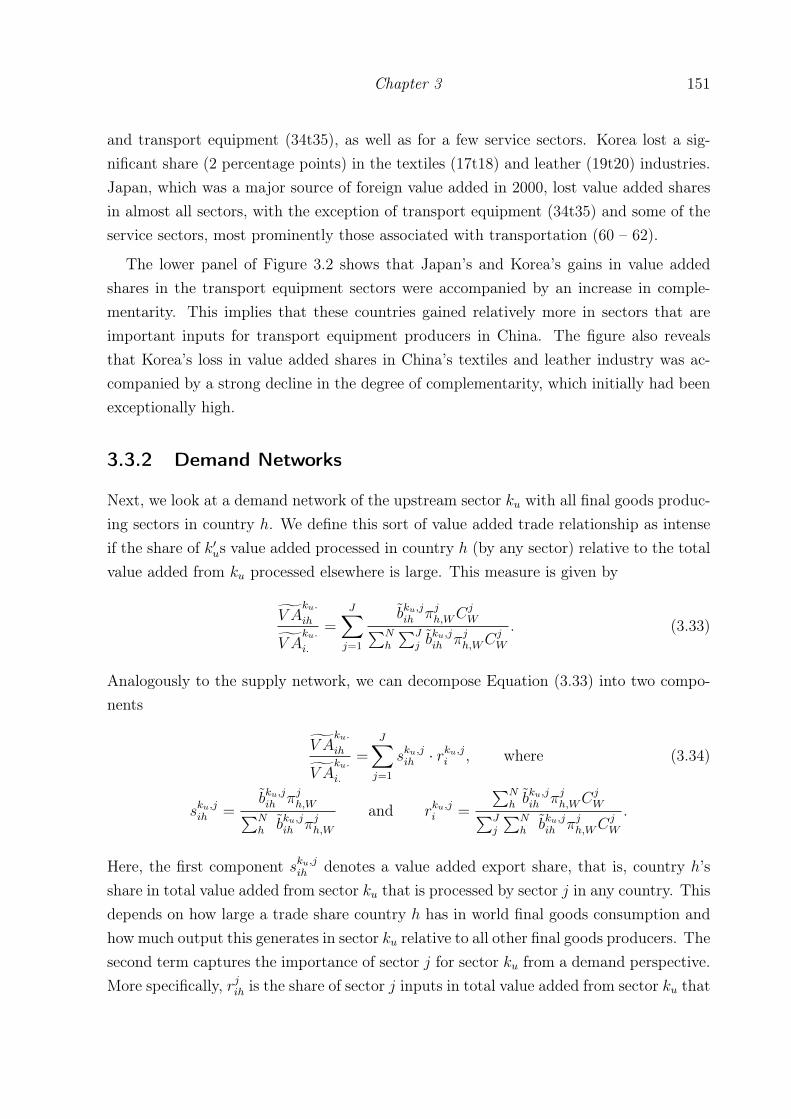
Chapter 3 151
and transport equipment (34t35), as well as for a few service sectors. Korea lost a sig-nificant share (2 percentage points) in the textiles (17t18) and leather (19t20) industries.Japan, which was a major source of foreign value added in 2000, lost value added sharesin almost all sectors, with the exception of transport equipment (34t35) and some of theservice sectors, most prominently those associated with transportation (60 – 62).
The lower panel of Figure 3.2 shows that Japan’s and Korea’s gains in value addedshares in the transport equipment sectors were accompanied by an increase in comple-mentarity. This implies that these countries gained relatively more in sectors that areimportant inputs for transport equipment producers in China. The figure also revealsthat Korea’s loss in value added shares in China’s textiles and leather industry was ac-companied by a strong decline in the degree of complementarity, which initially had beenexceptionally high.
3.3.2 Demand Networks
Next, we look at a demand network of the upstream sector ku with all final goods produc-ing sectors in country h. We define this sort of value added trade relationship as intenseif the share of k′us value added processed in country h (by any sector) relative to the totalvalue added from ku processed elsewhere is large. This measure is given by
V Aku.
ih
V Aku.
i.
=J∑j=1
bku,jih πjh,WCjW∑N
h
∑Jj b
ku,jih πjh,WC
jW
. (3.33)
Analogously to the supply network, we can decompose Equation (3.33) into two compo-nents
V Aku.
ih
V Aku.
i.
=J∑j=1
sku,jih · rku,ji , where (3.34)
sku,jih =bku,jih πjh,W∑Nh bku,jih πjh,W
and rku,ji =
∑Nh b
ku,jih πjh,WC
jW∑J
j
∑Nh bku,jih πjh,WC
jW
.
Here, the first component sku,jih denotes a value added export share, that is, country h’sshare in total value added from sector ku that is processed by sector j in any country. Thisdepends on how large a trade share country h has in world final goods consumption andhow much output this generates in sector ku relative to all other final goods producers. Thesecond term captures the importance of sector j for sector ku from a demand perspective.More specifically, rjih is the share of sector j inputs in total value added from sector ku that

152 Where is the Value Added? Trade Liberalization and Production Networks
Figure 3.3: Demand networks with China, 2000
010
2030
40sh
are
of C
hina
in V
A p
roce
ssed
(in
%)
-.4
-.2
0.2
.4co
rrel
atio
n co
effic
ient
AtB C 15t16 17t18 19 20 21t22 23 24 25 26 27t28 29 30t33 34t35 36t37 60 61 62 63 J 70 71t74
90 % of source countries JPN KOR USA CHN
Note: The figure plots demand networks as given in Equation (3.33) (upper panel) andthe correlation coefficient corresponding to the covariance in Equation (3.35) (lowerpanel). Calculations based on WIOD. Sectors on x-axis in Isic Rev. 3.
is processed in final goods consumption by all sectors in all countries. As for the supplynetwork, we can distinguish between two determinants of demand network strength basedon
V Aku.
ih
V Aku.
i.
=1
J
J∑j
sku,jih + J · Cov[sku,jih , rku,ji
]. (3.35)
This decomposition shows that the value added trade relationship is strong if country h isan important destination for country i on average, and particularly strong if, on average,country h captures a large share of sector ku’s value added in sectors that absorb a largeshare of value added from sector ku due to either technological reasons or to high demandfor this sector’s final goods.
We now describe demand networks with China. A demand network, as defined inEquation (3.33), captures the relative importance of a final goods producing country,here China, for an upstream sector in a specific source country. The upper panel ofFigure 3.3 shows that in 2000, for most countries, China was an important location forprocessing value added from the textiles (17t18) and leather (19t20) sectors, as well asfrom chemical products (24) and electronic and optical equipment (30t33), into finalgoods. It also shows the remarkable importance of China as a final goods producer for

Chapter 3 153
Figure 3.4: Demand networks with China, change 2000 – 2007
-10
010
20C
hang
e in
VA
sha
re (
in %
pts
)-.
20
.2.4
.6C
hang
e in
cor
rela
tion
coef
ficie
nt
AtB C 15t16 17t18 19 20 21t22 23 24 25 26 27t28 29 30t33 34t35 36t37 60 61 62 63 J 70 71t74
90 % of source countries JPN KOR USA CHN
Note: The figure plots changes in supply networks as given in Equation (3.33) (upper panel)and the correlation coefficient corresponding to the covariance in Equation (3.35) (in units,lower panel). Calculations based on WIOD. Sectors on x-axis in Isic Rev. 3.
Korean upstream sectors. With an average share of 5% across sectors, Korea was infact the country relying most heavily on processing in China, followed by Indonesia andAustralia, both having shares of about 2.5%. Japan is found in the middle or at the lowerend of the distribution of source countries in most sectors, except for textiles (17t18),metals (27t28) and electrical and optical equipment (30t33), in which sectors its relianceon China as a final goods producer was relatively strong.
The lower panel of Figure 3.3 reveals that the complementarities in demand networksare similar to those found for supply networks. Chinese upstream sectors exhibit strongcomplementarities with the sourcing structures of its downstream sectors, while for theupstream sectors in foreign countries, the correlation tends to be negative. This suggeststhat China’s reliance on domestic value added from the upstream sectors that are in-tensively used in important final goods industries was still relatively high. The limitedtradability of service sectors plays a crucial role here as well.

154 Where is the Value Added? Trade Liberalization and Production Networks
Figure 3.4 shows the changes in the demand networks and in complementarity. Between2000 and 2007, China’s importance as a processing location grew for almost all countriesand in almost all sectors. The electronic and optical equipment sector (30t33), as well asthe machinery sector (29), are particularly noteworthy in this regard. Furthermore, wefind that for both Japan and Korea, reliance on China increased particularly strongly formost sectors. China lost importance for Korea’s value added from the textiles (17t18)and leather (19t20) sectors. The figure’s lower panel shows increasing complementaritybetween foreign source sectors and the demand structure of China’s final goods sectors.This means, for example, that for the electrical and optimal equipment sector, strongerreliance on China as a processing location was particularly pronounced in sectors that userelatively more electrical and optical equipment as an input to production.
The deepening of networks with China suggests that China’s integration into the globaleconomy brought about a shift toward more foreign value in Chinese final goods andtowards all countries processing relatively more value added in China than elsewhere.Moreover, the increase in the complementarity measures indicates a change in the relativesupply structure toward more competitive sources and a change in the relative demandstructure toward more competitive final goods sectors. These findings highlight the scopefor gains achievable from specialization along the global value chain and, furthermore,illustrate that cross-sectoral dependencies play a crucial role in understanding how struc-tural changes affect countries’ relative competitiveness and how the effects of trade policyspread across all countries involved in global production sharing.
Before we evaluate China’s accession to the WTO by means of a counterfactual ex-periment, we first describe our data sources and how we identify the parameters of themodel.
3.4 Data and Parameter Identification
To simulate the effects of changes in tariffs, we need to identify the model parametersα, β, γ, and θ, and collect data on bilateral trade shares, tariff levels, countries’ totalvalue added, and trade surpluses. The expenditure shares α and the cost shares β andγ are obtained from input-output tables. θ is estimated as a trade cost elasticity basedon a structural equation that follows from the model. We obtain an alternative set ofestimates based on a standard gravity equation.

Chapter 3 155
3.4.1 Data Sources
Our main data source is the World Input-Output Database (WIOD), which providesharmonized international input-output tables as well as production values, final and in-termediate goods trade, and consumption by use categories. The database contains datafor 40 countries (mainly members of the OECD) and a rest-of-the-world aggregate (RoW)for the years 1995-2011, with a sectoral breakdown at roughtly the two-digit level of ISIC,resulting in 35 industries.15 The WIOD contains information on trade by sector, includingservices industries. The WIOD does not have information on actual bilateral input-outputcoefficients. These coefficients are imputed from national input-output tables based ona proportionality assumption. Accordingly, a sector’s usage of a certain intermediateinput is split between trade partners according to their respective shares in total inter-mediate goods imports. See Timmer (2012) for an in-depth description of methods andassumptions used to construct the WIOD.
Data on bilateral tariffs for manufacturing sectors are taken from UNCTAD’s TRAINSdatabase.16 We use effectively applied tariffs at the six-digit level of the HarmonizedSystem goods classification and aggregate them to the WIOD sectoral level using importvalues as weights. Other trade cost variables for our auxiliary gravity estimation, that is,bilateral distance and a dummy for contiguity, are obtained from the CEPII database. AFTA dummy is constructed based on the RTA database of the WTO.
3.4.2 Identification of Sectoral Productivity Dispersion
The sectoral productivity dispersion parameters are identified with the method proposedby Caliendo and Parro (2015). The estimation equation is based on a structural expressionfor gross trade flows derived from the model. By dividing a country-pair’s trade flow withtrade flows of other trade partners, importer, exporter, and pair-specific symmetric effectsare canceled out. The corresponding estimation equation is
lnXjinX
jhiX
jnh
XjniX
jihX
jhn
= − 1
θjln
(τ jinτ
jhiτ
jnh
τ jniτjihτ
jhn
)+ εjinh, (3.36)
15Due to lack of tariff data for Taiwan, we merge it with RoW and are thus left with 39 countries plusthe RoW aggregate.
16The database can be accessed via the World Bank’s World Integrated Trade Solution (WITS) project,https://wits.worldbank.org/WITS/WITS/Restricted/Login.aspx?AspxAutoDetectCookieSupport=1.

156 Where is the Value Added? Trade Liberalization and Production Networks
where εjinh is an i.i.d. error term. Identification rests on the assumption that unobservedtrade costs are exogenous to tariffs after differencing out all importer-sector-, exporter-sector-, and importer-exporter-specific effects.
Alternatively, we can identify θ from a standard gravity equation; the coefficient oftariffs in the gravity equation is 1/θj (see Equation (3.4)). Tariff data is directly observ-able, but iceberg trade costs are not. To estimate Equation (3.4), the gravity literaturetypically assumes a functional form for iceberg trade costs based on proxies such as bilat-eral distance and dummies for contiguity and joint membership in a free trade agreement(FTA). We proceed accordingly by assuming that djin = Din
ρj eδjZin , where Din is bilat-
eral distance and Zin is a vector collecting dichotomous trade cost proxies (contiguity andFTAs). Plugging this functional form into the trade share equation (3.4) and multiplyingby Xj
n, results in the following log-linearized estimable gravity equation for each sector j:
ln(πjinXjn) = − 1
θjln τ jin −
ρj
θjlnDin −
δj
θjZin + νji + µjn + εjin, (3.37)
where νji ≡ ln(λjicji ) is an exporter fixed effect, µjn ≡ ln(Xj
n/∑N
i=1 λji
[cjiκ
jin
]−1
θj ) is animporter fixed effect, and εjin an i.i.d. error term.
Table 5.1 displays the results from both estimation strategies. Each row corresponds toa separate estimation. Columns (1) and (2) show the estimates for the (inverse) produc-tivity dispersion, 1/θj, from the Caliendo and Parro (2015) methodology; in column (2)we drop from the sample the 0.5% of observations with the highest tariffs. Column (3)applies a gravity equation where importer and exporter fixed effects control for unob-served country-level heterogeneity and the log of distance and dummies for FTAs andfor contiguity proxy trade costs. Sectors are sorted in descending order of the estimatedcoefficient on tariffs. The higher 1/θj, the smaller the productivity dispersion in therespective sector. The coefficients are fairly stable across the different estimation proce-dures. Not surprisingly, “basic metals and fabricated metal,” “mining and quarrying,” and“coke, refined petroleum, and nuclear fuel” are at the top of the list. These sectors arecharacterized by more homogeneous products. At the lower end of the table are sectorssuch as “transport equipment” and “manufacturing nec.” which tend to produce more het-erogeneous goods. All in all, the sorting of sectors seems plausible.17 Also, the order ofmagnitude of the estimated coefficients seems plausible, except for three (two) estimatesthat are smaller than one in Column (1) (Column (2)). For our counterfactual analysis
17The estimates indicate that the agricultural sector has a rather high productivity dispersion. This isunexpected. However, given that this sector aggregates agriculture, hunting, forestry, and fishing, thisresult might be due to an aggregation bias.

Chapter 3 157
we use the estimates from Column (2), since Caliendo and Parro (2015)’s methodologyrelies on weaker identification assumptions. For "manufacturing nec." we use the gravityestimate.
Data on bilateral tariffs are not available for service sectors. Therefore, we cannotapply our estimation strategy for sectors listed in ISIC Chapters E-Q. Instead, we rely onan average value obtained by Egger et al. (2012), who estimate a trade cost elasticity forservices of 5.959.
3.4.3 Expenditure and Cost Shares
The remaining parameters, α, β, and γ, and the trade shares π, are obtained from WIODin conjunction with the tariff data described above. We match production values, thesectoral bilateral trade flows (aggregating intermediate and final goods trade), and thecost shares for intermediates from the WIOD as well as the tariff structure in 2000. Wecalculate value added, final goods expenditure, and the trade surplus by applying theequilibrium conditions of the model. We show below that deviations from the empiricalcounterparts are not substantial.
The WIOD data are valued in producer prices; we obtain bilateral imports in purchaserprices by applying the add-valorem tariffs to the reverse export flows so that Xk
in =
Zkin(1 + τ kin). Trade shares are then computed as
πkin =Xkin∑N
i=1Xkin
.
Sectoral value added for each country is obtained by subtracting the total cost ofintermediate usage from the sector’s production value. To that end, we first need toconvert sector j’s usage of intermediate inputs to purchaser prices by adding the expensesfor tariffs to the fob value. Tariff expenses can be calculated as follows:
TF jn =
∑i
∑k
πkinτ kin
τ kin + 1(1− βjn)γk,jn Y j
n
where (1− βjn)γk,jn =∑i ak,jin
Fknand the value of production observes Y j
n =∑N
i Zkni + ∆Invjn,
that is, it is given by the sum over exports plus changes in the stock of inventory. Value

158 Where is the Value Added? Trade Liberalization and Production Networks
Table 3.1: Gravity estimates of sectoral dispersion parameter
(1) (2) (3)ISIC Rev. 3 Sector Estimates of −1/θ
CP CP (99.5) FE27-28 Basic metals -12.3572*** -14.5695*** -12.7967***
(0.2050) (0.2232) (0.9444)C Mining, quarrying -12.0365*** -13.7911*** -12.2792***
(0.7800) (0.8951) (1.8261)23 Coke, petroleum -11.0537*** -11.4946*** -7.5495***
(1.4409) (1.6248) (2.5559)24 Chemicals -9.7762*** -11.2670*** -9.3409***
(0.2220) (0.2416) (0.8369)20 Wood -11.1967*** -10.7237*** -10.7012***
(0.2924) (0.3026) (0.9028)26 Non-metallic minerals -2.8295*** -6.1282*** -6.1251***
(0.2866) (0.2397) (1.5628)19 Leather -3.9975*** -5.5967*** -5.6334***
(0.1529) (0.1798) (0.7012)17-18 Textiles -5.2900*** -5.2978*** -5.1851***
(0.1191) (0.1205) (0.5769)21-22 Paper -4.4812*** -4.4347*** -5.3701***
(0.2177) (0.2333) (0.7306)29 Machinery nec. -4.6152*** -4.2234*** -4.5264***
(0.2201) (0.2365) (0.7764)15-16 Food -1.7676*** -2.8780*** -2.0467***
(0.0600) (0.0669) (0.3212)30-33 Electrical equip. -3.2876*** -2.5285*** -4.4546***
(0.1847) (0.1910) (0.7313)25 Rubber -1.5353*** -2.0934*** -2.6653***
(0.2094) (0.2286) (0.7344)A-B Agriculture -0.4081*** -1.4012*** -1.4457***
(0.0606) (0.1043) (0.3115)34-35 Transport equip. -0.8259*** -0.9790*** -1.9491***
(0.1831) (0.2190) (0.6332)36-37 Manufacturing nec. -0.7979*** -0.6021*** -2.7715***
(0.1579) (0.1621) (0.6876)# Observations 1,146,618 1,126,494 93,691# Exporters/ # Importers 212/120 212/120 212/120
Note: The table shows estimates for the (inverse) sectoral productivity dispersion 1/θ as identified bya cross-sectional gravity estimation for the year 2007. Columns (1) and (2) apply the Caliendo-Parro(CP) method as given in Equation (3.36), Column (3) applies the gravity equation with importerand exporter fixed effects (FE) and controls for bilateral trade costs as given in Equation (3.37).Column (2) drops from the sample the 0.5% highest tariffs. Sectors are sorted in descending orderof the estimated coefficient in Column (2). Standard errors (in parentheses) are heteroskedasticity-robust. *, ** and *** indicate statistical significance at the 10, 5, and 1% level, respectively.

Chapter 3 159
Figure 3.5: Model fit: Final goods trade
020
000
4000
060
000
8000
010
0000
Fin
al g
oods
trad
e W
IOD
(in
mio
usd
)
0 20000 40000 60000 80000 100000
Final goods trade model (in mio usd)
Note: The figure plots bilateral sectoral final goods expenditures in 2000 implied bythe model (x-axis) against their counterpart in the data (y-axis, WIOD).
added then results from subtracting the total cost of intermediate usage from the sector’sproduction value, that is,
V Ajn = Y jn −
J∑k
N∑i
ak,jin Yjn − TF j
n.
Value added shares β follow as βjn = V AjnY jn
. The cost shares for intermediate inputs,
γk,jn , can be backed out from (1− βjn)γk,jn =∑i ak,jin
Fknusing the βjn’s.
The share of expenditure on goods from sector k in total final goods consumption,αkn, is derived from the sectoral goods market clearing condition, which requires totalexpenditure on goods from sector k, Xk
n =∑N
i=1 Xkin, to be equal to the sum of expenditure
on intermediate and final goods and thus results as
αkn =Xkn −
∑Jj (1− βjn)γk,jn Y j
n
In.

160 Where is the Value Added? Trade Liberalization and Production Networks
Finally, income is pinned down by a macroeconomic closure condition that requires incometo be equal to final goods expenditure, In =
∑kX
kn −
∑k
∑j(1− βjn)γk,jn Y j
n , and followsas
In = V An +Rn − Sn −∆Invn,
where Sn is the aggregate trade surplus (net exports)∑N
i Zkni −
∑Ni Z
kin and ∆Invn is
the net change in inventories. Both terms appear as a mere transfer of income in ourone-period setting. The trade surplus is valued in producer prices, since tariff income iscaptured separately in Rn.
To compute final goods consumption and trade we imposed the assumption inherentto the model that bilateral trade shares are the same for final and intermediate goods.Figure 3.5 plots the model-based sectoral bilateral final goods expenditures versus theactual data from WIOD (56,000 observations).18 The deviations are minor, suggestingthat the assumption is not problematic.19
3.5 Counterfactual Analysis: China’s WTO Accession
3.5.1 Developments in China’s Export Composition and BilateralValue Added Trade Relationships in the 2000s
China’s accession to the World Trade Organization (WTO) in 2001 was a major tradeshock. It is widely believed that it significantly changed global sourcing structures andhas spurred formation of production networks with China. Most notable in the latterregard is the evolution of an Asian production network in which Japan and Korea andother Asian countries supply intermediates to China where they are assembled into finalgoods. China then exports the final goods, predominantly to the United States, but alsoto the European Union. Between 2000 and 2008, China’s real exports increased by afactor of 4.7, which implies an increase in the share in world exports from 4 to almost10 percent. This surge in exports was accompanied by an almost concurrent decline inthe domestic value added content. Figure 3.6 shows China’s total exports (right scale)and the value added composition (left scale). The share of value added contributed byChina to its own exports decreased steadily. In 2000, foreign value added accounted for14 percent of the value of Chinese exports; in 2008 its share was 22 percent. The increase
18The largest .01 percent of observations have been omitted from Figure 3.5 for display purposes.19The largest outlier is the U.S. domestic expenditure share for textiles, where the model overestimatesthe data by 35 percent. The other apparent outliers all involve RoW.

Chapter 3 161
Figure 3.6: China’s exports to the world and their value added composition
050
010
0015
00E
xpor
ts in
bill
. US
D (
cons
tant
, yea
r 20
00)
0.1
.2.3
VA
sha
re in
tota
l exp
orts
(cu
mul
ativ
e)
1996 1998 2000 2002 2004 2006 2008
Foreign VA Double counting
Returned dom. VA (sum) exp
Note: The figure shows the evolution of China’s export (dashed line, right scale) and thecumulated shares of returned domestic value added, double counted value added, and foreignvalue (left) scale. Shares were computed based on methodology developed by Koopman etal. (2014).
in the share of double-counted trade from 3 to 7.5 percent over the same period is furtherevidence of China’s deepening integration into the global value chain.20
The increase in the foreign value added content of China’s exports is reflected in largedeviations of bilateral trade balances from net value added trade flows. The left panel ofFigure 3.7 shows the U.S. trade balance with China. During the whole period 1995 to2009, the U.S. ran a trade deficit with China. With China’s accession to the WTO, thisdeficit greatly increased. Starting at about 0.5% of U.S. GDP in 2001, U.S. net importsfrom China almost quadrupled to 2% of U.S. GDP by 2007. However, the increase in netvalue added transfers from China to the United States was much smaller. In the same timeperiod, these increased from around 0.5% of U.S. GDP to only 1.5%. This implies thatthe U.S. trade deficit with China is considerably overstated when measured in gross termsinstead of value added terms. In 2007, the trade deficit was overestimated by about 25percent. Over the same period, Japan’s net direct export to the United States decreased,
20We use Koopman et al. (2014)’s methodology (described above) to compute those shares using datafrom the WIOD. The share of domestic value added in exports that is consumed abroad is given by oneminus the cumulated shares of foreign value added, double-counting, and domestic value that returnshome.

162 Where is the Value Added? Trade Liberalization and Production Networks
Figure 3.7: U.S. trade deficit with China and Japan
*
1520
2530
35D
iffer
ence
in %
-.8
-.6
-.4
-.2
Net
(V
A)
expo
rt in
% G
DP
1996 1998 2000 2002 2004 2006 2008
China
-50
-40
-30
-20
-10
Diff
eren
ce in
%
-.4
-.3
-.2
-.1
0N
et (
VA
) ex
port
in %
of G
DP
1996 1998 2000 2002 2004 2006 2008
Japan
VA export Exports Difference in %
Note: The figure shows the evolution of U.S. net exports (light gray bars) and net value added exports(dark gray bars) to China (left panel) and Japan (right panel) as a share of U.S. GDP for the period1995-2009. The figure also shows the adjustment of the deficit from value added terms to nominal exportsterms (dashed line, right scale).
while net value added transfers went up (see right panel of Figure 3.7). In value addedterms, the U.S. trade deficit with Japan was understated by around 35 percent in 2007.
As shown in our empirical section on networks, China was by far the most importantforeign destination for Japan and Korea in terms of processing their value added into finalgoods and, at the same time, these countries were among the most important sources offoreign value added for China. Korea also experienced disproportionally strong growthin the demand and supply networks, and even though Japan lost in terms of relativeimportance as a source country for China, the latter’s importance as a processing countryfor Japanese value added increased disproportionately.
3.5.2 China’s Accession to the WTO in 2001
To what extent can we attribute these observations to China’s accession to the WTO?Can the WTO entry explain the increase in production fragmentation, China’s rise as afinal goods exporter, and the network formation with its neighboring countries?
To answer these questions, we calibrate the model to the year prior to the accession(2000) and then simulate China’s entry by changing China’s inward and outward tariffrates with respect to all other countries to the level observed in 2007. Table 3.2 shows the

Chapter 3 163
Table 3.2: Inward and outward tariffs with China in 2000 and changes to 2007
Inward Outward Inward OutwardCountry Tariff % Cut Tariff % Cut Country Tariff % Cut Tariff % CutBRA 13.1 -2.7 35.7 -17.2 NLD 0.9 -0.1 6.0 -3.1USA 4.1 -0.4 15.4 -7.1 POL 2.5 -0.3 5.9 -3.0MEX 17.0 -6.4 11.7 -6.7 TUR 7.8 -4.5 10.2 -3.0IDN 4.7 -1.5 11.8 -6.6 GBR 2.3 -0.2 5.0 -2.8JPN 3.2 0.0 14.1 -6.5 AUT 2.2 -0.2 4.6 -2.5RoW 8.2 -5.2 11.9 -6.4 ITA 2.9 -0.2 5.0 -2.5KOR 5.8 -1.6 13.5 -6.0 RUS 11.1 -0.8 5.9 -2.5CAN 4.8 -0.3 11.3 -5.9 BEL 2.1 -0.2 5.3 -2.5DNK 2.4 -0.1 10.4 -5.5 CZE 2.9 -0.3 5.1 -2.0CYP 3.5 -0.2 10.8 -5.0 SVK 2.6 -0.2 4.9 -2.0LTU 2.8 -0.2 8.3 -4.2 LVA 2.9 -0.2 4.6 -1.9IND 26.6 -1.3 11.2 -3.9 BGR 1.8 -0.4 4.8 -1.9FIN 1.7 -0.3 5.8 -3.7 SVN 2.5 -0.3 3.0 -1.4IRL 1.5 -0.3 5.9 -3.5 ESP 2.8 -0.2 2.6 -1.3EST 2.1 -0.4 6.7 -3.3 GRC 2.9 -0.2 3.4 -1.2FRA 2.5 -0.3 5.9 -3.2 MLT 3.1 -0.2 1.5 -1.0HUN 1.7 -0.4 5.2 -3.2 ROU 3.1 -0.3 1.9 -0.8AUS 22.0 -5.1 12.9 -3.2 PRT 2.4 -0.2 1.2 -0.6SWE 3.0 -0.3 4.6 -3.1 LUX 1.0 0.0 0.4 -0.2DEU 2.5 -0.3 5.4 -3.1
Note: The table shows trade-weighted average tariffs and tariff changes for all countries with respectto China
magnitude of the tariff cuts for the countries in our sample. The cuts were substantial, butvery heterogeneous across countries; import tariffs on goods from China decreased mostfor Mexico and Australia, where initial levels were also very high. On the other hand,China had to drastically cut its tariffs on imports from the North American economies(the United States, Mexico, and Canada) and on those from its neighboring countriesJapan and Korea, as well as those from the emerging economies of Brazil, Indonesia, andIndia, and the mostly developing countries grouped in the RoW aggregate.
As regards sectoral heterogeneity, Table 3.3 shows that tariff cuts were particularlydeep in the “food, beverages and tobacco” sector and in agriculture, but also for “trans-port equipment,” “manufacturing, nec” and “electrical and optical equipment.” For thosesectors, the magnitude of tariff cuts also varied substantially across trade partners. Giventhe large heterogeneity across both sectors and countries, we do not expect all countriesto benefit equally from China’s WTO entry.

164 Where is the Value Added? Trade Liberalization and Production Networks
Table 3.3: Sectoral tariff changes, 2000-2007
ISIC Sector Tariff Cut Std.Dev.(in %)
15+16 Food, beverages and tobacco -21.1 66.1A+B Agriculture, hunting, forestry and fishing -11.6 25.734+35 Transport equipment -6.6 8.536+37 Manufacturing, nec; recycling -6.2 6.230-33 Electrical and optical equipment -5.1 3.517+18 Textiles and textile products -4.9 5.325 Rubber and plastics -4.6 3.8
21+22 Pulp, paper, printing and publishing -4.4 3.524 Chemicals and chemical products -4.0 4.129 Machinery, nec. -4.0 3.523 Coke, refined petroleum and nuclear fuel -3.8 11.120 Wood and products of wood and cork -3.6 4.219 Leather and footwear -3.3 3.126 Other non-metallic mineral -3.3 3.7
27+28 Basic metals and fabricated metal -3.0 2.9C Mining and quarrying -0.8 1.1
Note: The table shows average tariff changes by sector (in %) with respect to China between2000 and 2007 and the corresponding standard deviation.
3.5.3 Results: The Effect of China’s WTO Entry
3.5.3.1 Aggregate Trade and Welfare Effects
Our counterfactual analysis predicts that world real exports increased by 2.1% due toChina’s WTO entry and that world trade over world production went up by .23 percentagepoints, as we show in Table 3.4. The driving force behind this overall increase was, ofcourse, China itself, for which we find an increase in total exports of 28 %. A sizeable effectcan also be attributed to Australia (19%). Much smaller but still significant increaseswere experienced by China’s neighboring countries Korea, Indonesia, and Japan. Wefind positive but small trade effects for the United States and negligible or even slightlynegative effects for most of the European economies. Furthermore, the results show thatChina’s WTO entry did indeed spur production fragmentation. China’s value addedexports increased by much less than its total exports. This is indicated by China’s valueadded to export ratio, which decreased by 4 percentage points. On the world level, theVAX ratio decreased by 0.3 percentage points. We find decreasing ratios also for theother countries that had positive export changes. Interestingly, for many countries withnegative export effects, value added exports increased by less.
How big are these predicted changes in relation to the actual changes that occurredbetween 2000 and 2007? The answer to this question depends very strongly on the

Chapter 3 165
Table 3.4: Aggregate trade effects
Counterfactual Change Actual Change 2000-2007
Country Rank X X X/Y V AX/X X X/Y V AX/X% % pts % pts % % pts % pts
CHN 1 28.35 2.49 -3.87 307 3.55 -9.13AUS 2 19.28 2.47 -1.92 83 -0.83 -1.69KOR 3 3.34 0.44 -0.71 87 0.68 -4.04RoW 4 2.39 0.37 -0.60 100 3.04 -6.08IDN 5 1.73 0.30 -0.34 62 -4.44 2.93JPN 6 1.52 0.08 -0.20 28 3.19 -7.19BRA 7 1.38 0.08 -0.05 140 1.81 -0.37USA 8 0.42 0.02 0.01 32 0.57 0.32IND 9 0.39 0.04 -0.12 204 2.87 -5.63RUS 10 0.17 0.04 -0.04 182 -7.31 1.64
ROU 31 -0.18 -0.01 0.05 257 -0.67 -1.23EST 32 -0.19 -0.02 0.02 154 -4.04 5.50POL 33 -0.19 -0.01 0.01 218 5.87 -7.52CZE 34 -0.19 -0.02 0.02 236 5.18 -7.66MLT 35 -0.20 -0.01 0.03 58 -2.71 7.12ESP 36 -0.20 -0.01 0.00 101 -0.97 -3.03SVN 37 -0.22 -0.02 0.02 152 5.05 -4.69ITA 38 -0.23 -0.01 0.01 79 0.93 -4.46PRT 39 -0.34 -0.03 0.02 89 1.51 -2.09LTU 40 -0.58 -0.08 -0.03 237 2.60 1.59
WLD 2.10 0.23 -0.28 86 2.49 -3.81
Countries ranking 11-30 in terms of changes in exports not shown.
particular numbers at which we look. On the world level, we find that China’s WTOentry explains about 9% of the increase in world exports relative to world GDP andabout 7% of the decline in the world VAX ratio. These are sizeable effects if one takesinto account that the only difference between the baseline scenario and the counterfactualis the tariff schedule of one country. The scenario does not consider growth in worldGDP or growth in China due to anything other than the tariff changes, which explainswhy the counterfactual changes in total world exports or China’s exports explain only amarginal fraction of the actual change (about .25% for the world and 10% for China).As regards China’s growth in exports over GDP or value added exports over exports, thecontribution of the WTO entry is much larger. About 2.5 percentage points (70%) of the3.5 percentage point increase in exports over GDP and 4 percentage points (45%) of the 9percentage points decrease in the VAX ratio can be attributed to the change in the tariffstructure.

166 Where is the Value Added? Trade Liberalization and Production Networks
Table 3.5: Changes in export composition (in % pts)
Exporter VA Exports VA Reimports Foreign VA Double Counting TariffsCHN -3.87 0.31 1.26 3.08 -0.78AUS -1.92 0.11 0.40 1.70 -0.30KOR -0.71 0.03 0.52 0.21 -0.05RoW -0.60 0.08 0.32 0.29 -0.08IDN -0.34 0.00 0.20 0.16 -0.02JPN -0.20 0.05 0.10 0.06 -0.01IND -0.12 0.00 0.09 0.02 0.01WLD -0.28 0.01 0.15 0.18 -0.05
Note: The table shows the changes in the composition for the seven countries with the largest declinesin the VAX-ratio.
China’s WTO entry also explains a large share of the actual developments in Australia.About one-fourth of Australia’s increase in total exports and almost 90% of the declinein its VAX ratio can be explained by the WTO entry, although the fact that exportsover GDP actually declined implies that other significant changes were happening inAustralia that cannot be explained by China’s trade integration. For Japan’s and Korea’saggregate statistics we find that the changes implied by our counterfactual point in thesame direction as the actual changes, but the share explained by the counterfactual issmall, especially for Japan. Not surprisingly, the farther away we move from China,the less of the actual development is explained. However, as we show below, on a moredisaggregated level we find that China’s WTO entry significantly influenced the bilateraland sectoral pattern of trade in value added.
Next, we use the decomposition method outlined above to analyze how China’s WTOentry affected the composition of countries’ exports. In Table 3.5 we show the worldaggregate for comparison and the countries with the largest declines in their VAX ratios,which are, except for RoW, all countries geographically close to China. We find forChina that the largest part of the decline in the domestic value content was due toan increase in the share of double-counted value added, which increased by 3 percentagepoints. In comparison, the share of foreign value added increased by 1.7 percentage points.Australia’s exports experienced similar changes in composition; for the other countries,the increase in the share of foreign value added exceeded the increase in double-counting.
Figure 3.8 shows how the pattern of world wide value added sourcing changed between2000 and 2007 and what part of this can or cannot be explained by China’s WTO ac-cession. The dark gray bars show the actual changes and the light gray bars show thechanges to the counterfactual equilibrium. We group the countries that exhibited qual-

Chapter 3 167
Figure 3.8: Changes in world value export shares
-5-2
.50
2.5
5C
hang
e in
sha
re in
wor
ld V
A e
xpor
ts (
in %
pts
.)
AUS Asia BRIT CHN EEC EU1 EU2 NA RoW
Counterfactual change Actual change 2000-2007
Countries are grouped as follows: Asia: IDN, JPN, KOR; BRIT : BRA, RUS,IND, TUR; EEC : Eastern Europe; EU1 : AUT, DEU, LUX, IRL, ESP, POR;EU2 : BEL, DNK, FIN, FRA, GBR, ITA, NLD, SWE: NA: CAN, USA, MEX
itatively similar changes both in the counterfactual and in the actual data and we findthat this scheme is in good accordance with a grouping based solely on geography. Be-tween 2000 and 2007, China gained a significant share in total world value added exports,reaching 9.5% in 2007. Furthermore, Australia, a group of western European countries(EU1), and the central and eastern European countries (EEC), as well as the emergingcountries (BRIT) and the primarily developing countries in RoW, were able to increasetheir shares in world value added exports. This came at the expense of a second set ofwestern European countries and the North American and Asian industrialized economies.We find that China’s WTO entry can account for about 20% of its increase in the share ofworld value added. The country’s WTO entry did not significantly affect the shares of theother Asian economies, those of the emerging and eastern European countries, nor thoseof RoW. Apparently, the dynamics of those regions were due to something else. However,China’s WTO accession did contribute to the loss in value added export shares by thenorthern American and western European countries and the slight gains in Australia’sshare.

168 Where is the Value Added? Trade Liberalization and Production Networks
Table 3.6: Welfare changes (in %)
Country W (w/P ) P R Rank WAUS 2.62 3.18 -3.94 -28.23 1CHN 0.56 1.52 -1.27 -41.12 2KOR 0.24 0.23 0.31 -0.33 3IDN 0.13 0.14 -0.09 -1.65 4RoW 0.07 0.15 -0.08 -5.34 5JPN 0.04 0.03 0.11 2.71 6CYP 0.04 0.02 -0.07 -0.10 7MLT 0.04 0.02 -0.13 0.45 8BRA 0.03 0.03 0.09 0.39 9RUS 0.03 0.03 -0.05 0.11 10USA 0.02 0.02 -0.06 -0.50 13SVK 0.00 0.00 -0.11 -0.75 31FRA 0.00 0.01 -0.10 -0.69 32SVN 0.00 0.00 -0.12 -0.61 33ITA 0.00 0.00 -0.13 -0.09 34LUX -0.01 0.01 -0.09 -0.20 35BEL -0.01 0.00 -0.11 -0.66 36TUR -0.01 0.00 -0.22 -3.25 37IRL -0.01 0.02 -0.14 -1.28 38MEX -0.02 0.02 -0.11 -1.04 39LTU -0.04 -0.06 -0.20 -0.81 40
Note: The table shows counterfactual changes in welfare W (realincome), real wages (w/P ), the price level P , and tariff revenue Rfor the 10 most positively and most negatively affected countries interms of welfare as well as for the U.S..
To assess the welfare implications of China’s accession to the WTO we look at changesin real income as given in Equation (3.12). The two determinants of welfare changes arereal wages and tariff income. Due to global production linkages, real wages in all countriesare much more directly affected than just through the equilibrium price indices, as is thecase in the standard gravity model. Even countries that experienced little or no tariffchanges with respect to China can witness an increased demand for their labor if they arean important input supplier either for China or for some other country that experiencedsignificant changes in the tariff structure. Similarly, production linkages imply that othercountries’ production costs show up directly in a country’s own price index. Hence, weexpect that the welfare consequences are much more complex than in a standard generalequilibrium gravity framework without input-output linkages.
China’s WTO entry resulted in positive welfare gains in terms of a positive change inaggregate real income for China itself, and also for most other countries. Table 3.6 showswelfare changes for the 10 most and least positively affected countries and for the UnitedStates. Remarkably, Australia experienced the largest real income gain – 2.6 percentage

Chapter 3 169
points – more than four times the increase for China. Australia benefited from a strongdecrease in the price index, which compensated for the significant 28% decline in tariffrevenue. Similarly, China lost 41% of its tariff revenue, but also experienced a significantreduction in prices and higher demand for its labor, resulting in a net real income gainof .6%. The other countries with sizeable positive effects are China’s neighbors andthe mostly developing countries in the RoW aggregate. We find that in most countriesprices decreased, with the noteworthy exceptions of Japan and Korea, where the increaseddemand for labor drove up nominal wages and prices. Nevertheless, these two countriesstill experienced real wage gains. The increased demand for labor in Korea and Japansuggests that the relocation of production to China (which we document below for finalgoods production) was overcompensated by an increase in total demand. We also findpositive but small welfare effects for the United States, where the decline in the priceindex was sufficiently large to make up for the loss in nominal wages and tariff income.We find small negative welfare effects for only six countries, with Lithuania, the mostadversely affected country, experiencing a decline in real income of .04%.
A few comments are in order in regard to the welfare effects of our counterfactualexperiment. First, in our static framework trade deficits appear as one-time net incometransfers that are treated as exogenous and held constant when moving to the counter-factual equilibrium. Second, we assume perfect labor mobility across sectors within acountry. Since sectors were affected very differently, owing both to heterogeneous tariffcuts and different sourcing structures, the assumption of labor mobility clearly mattersfor whether countries could actually realize the real wage gains predicted by the model,and over what time horizon. And lastly, as mentioned before, the consequences of China’sWTO accession were much broader than those we discuss here. Our welfare effects reflectonly the changes induced by the tariff cuts.
3.5.3.2 Effects on Bilateral Trade in Value Added and Networks
Supply Networks. China’s WTO accession facilitated easier access to inputs for Chi-nese final goods producers. The sectoral and bilateral heterogeneity suggests that inputsuppliers were differentially affected, yet the sectoral and global interlinkages make it hardto ex-ante predict how value added flows change as a consequence of trade cost changes.We use our measure of supply networks to shed light on the question of which countriesand sectors intensified their production linkages with China.
Three features of value added trade relationships, when present, tended to make theserelationships particularly affected by China’s WTO entry. First, geographical proximity

170 Where is the Value Added? Trade Liberalization and Production Networks
Figure 3.9: Changes in the intensity of supply networks for selected countries
AUSAUS
AUSAUS
AUS
AUS
AUSAUS
AUS
AUSAUS
AUS
AUS
AUSAUS
AUS
JPN
JPNJPN
JPN
JPN
JPN
JPN
JPN
JPN
JPN
JPN
JPN
JPN
JPN
JPN
JPN
KOR
KOR
KOR
KOR
KOR
KOR
KOR
KORKOR
KOR
KOR
KOR
KOR
KOR
KOR
KOR
USAUSA
USA
USA
USA
USA USA
USA
USA
USA
USA
USAUSA
USA
USA
USA
0.5
11.
52
Cha
nge
in V
A s
hare
(in
% p
ts)
0 .02 .04 .06 .08
share in VA processed in China
AUSAUS
AUSAUS
AUS
AUS
AUS AUS
AUS
AUS AUS
AUS
AUS
AUSAUS
AUS
JPN
JPNJPN
JPN
JPN
JPN
JPN
JPN
JPN
JPN
JPN
JPN
JPN
JPN
JPN
JPN
KOR
KOR
KOR
KOR
KOR
KOR
KOR
KORKOR
KOR
KOR
KOR
KOR
KOR
KOR
KOR
USA USA
USA
USA
USA
USA USA
USA
USA
USA
USA
USAUSA
USA
USA
USA
0.5
11.
52
Cha
nge
in V
A s
hare
(in
% p
ts)
-.3 -.2 -.1 0 .1 .2
Correlation coefficient
Counterfactual change Fitted values
Note: The figure plots changes in supply network intensity as defined in Equation (3.30) againstvalues (left panel) and against the inital degree of complementarity (right panel), given by covari-ance term in Equation (3.32) standardized by the product of the standard deviations of πk,jd,V Aih
and γk,jd,V Ah .
was a major determinant. Following the RoW aggregate, Japan, Korea, Indonesia, andAustralia were the countries that on average experienced the strongest increases in theirshares of foreign value added processed by final goods sectors in China. Second, thescope and the depth of existing supply networks mattered. Figure 3.9 shows for China’sneighboring countries and the United States that the initial value added share was astrong predictor of the change in the share (left panel). Each dot is a supply networkbetween the country as labeled and one downstream sector in China. Likewise, a deepernetwork facilitated a stronger increase in the value added share (right panel), where thedepth of a supply network is measured by the correlation between the source country’srelative competitiveness in an upstream sector and the importance of that upstream sectorin general for the downstream sector in China.
Table 3.7 presents the correlations for all source countries and all downstream sectorsin China and compares the counterfactual changes to the actual changes. Columns (1)and (3) show the relationship of the change in the share with the initial level. Columns (2)and (4) display the relationship with each of the components of the supply network and

Chapter 3 171
Table 3.7: Determinants of changes in supply networks
Dep. var: ∆V A
.jdih
V A.jdi.
Counterfactual Actual Change
V A.jdih /V A.jdi. 26.46*** 17.72***
(0.354) (0.884)
πk,jd,V Aih 22.60*** 12.25***(0.307) (1.037)
ρ(πk,jd,V Aih , γk,jd,V Ah ) 0.289*** 0.480***(0.0397) (0.0740)
N 1287 1287 1287 1287R2 0.813 0.819 0.238 0.153
Note: The table shows OLS regression results for changes in supply networkintensity for all source countries with all downstream sectors in China. Stan-dard errors in parentheses. ∗ p < 0.1, ∗∗ p < 0.05, ∗∗∗ p < 0.01. ρ denotes thecorrelation coefficient; the other variables are as defined in Equation (3.35).
confirm that each has a separate effect on intensity of the network. The counterfactualchanges strongly resemble the pattern in the data. In terms of magnitudes, we find forthe counterfactual that a 1 percentage point higher initial value added share is associatedwith a .26 percentage point stronger increase. The actual data predict a .18 percentagepoint increase. An increase in the correlation coefficient by .01 units is associated witha .29 percentage point higher increase in the counterfactual and .48 in the data. It isnoteworthy that the initial strength of the network is a remarkably strong predictor ofthe counterfactual change, as indicated by an R2 larger than .8, and also has substantialexplanatory power for the changes that we observe in the data over a period of sevenyears.
We find a strong resemblance between the counterfactual changes and the actual datawithin sectors, too. Figure 3.10 plots for all source countries the changes in supplynetwork intensity with China’s manufacturing sectors (29-36) in the counterfactual againstthe change in the data. The majority of countries are clustered at zero both in ourcounterfactual and in the data. Countries that repeatedly stand out are Japan, Korea,Australia, the United States, Germany, and RoW. In many cases, the changes in thedata are very well explained by our counterfactual, especially so in the case of RoW,Australia, the United States, and Korea. These countries are aligned on or close to the45-degree line, which is the most challenging benchmark. Apparently, the counterfactualdoes not do well at explaining the developments in Japan, which lost value added sharesin those sectors or gained only a little, whereas our simulation suggests that China’s WTO
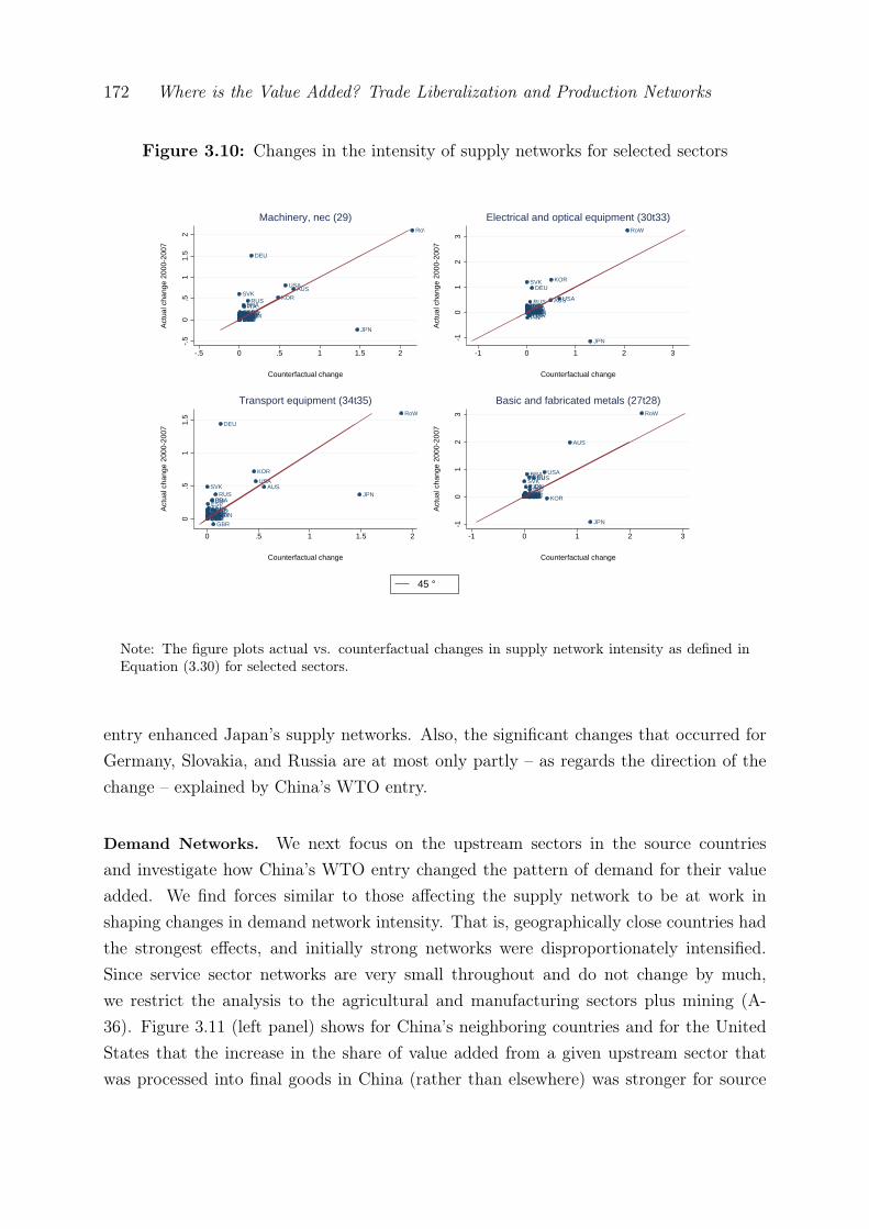
172 Where is the Value Added? Trade Liberalization and Production Networks
Figure 3.10: Changes in the intensity of supply networks for selected sectors
AUS
AUTBELBGR
BRACAN
CYPCZE
DEU
DNKESPESTFIN
FRAGBRGRCHUNIDNINDIRL
ITA
JPN
KOR
LTULUXLVAMEX
MLTNLDPOLPRTROU
RUS
RoW
SVK
SVNSWETUR
USA
-.5
0.5
11.
52
Act
ual c
hang
e 20
00-2
007
-.5 0 .5 1 1.5 2
Counterfactual change
Machinery, nec (29)
AUS
AUTBELBGRBRACANCYP
CZE
DEU
DNKESPESTFINFRAGBRGRCHUN
IDNINDIRLITA
JPN
KOR
LTULUXLVAMEXMLTNLDPOLPRTROU
RUS
RoW
SVK
SVNSWETUR
USA
-10
12
3
Act
ual c
hang
e 20
00-2
007
-1 0 1 2 3
Counterfactual change
Electrical and optical equipment (30t33)
AUS
AUTBELBGR
BRA
CANCYPCZE
DEU
DNK
ESP
ESTFINFRA
GBRGRCHUN
IDNIND
IRL
ITAJPN
KOR
LTULUXLVAMEX
MLT
NLDPOLPRTROU
RUS
RoW
SVK
SVNSWETUR
USA
0.5
11.
5
Act
ual c
hang
e 20
00-2
007
0 .5 1 1.5 2
Counterfactual change
Transport equipment (34t35)
AUS
AUTBELBGR
BRA
CAN
CYPCZE
DEU
DNKESPESTFINFRAGBRGRCHUNIDNIND
IRLITA
JPN
KORLTULUXLVAMEXMLTNLDPOLPRTROU
RUS
RoW
SVK
SVNSWETUR
USA
-10
12
3
Act
ual c
hang
e 20
00-2
007
-1 0 1 2 3
Counterfactual change
Basic and fabricated metals (27t28)
45 °
Note: The figure plots actual vs. counterfactual changes in supply network intensity as defined inEquation (3.30) for selected sectors.
entry enhanced Japan’s supply networks. Also, the significant changes that occurred forGermany, Slovakia, and Russia are at most only partly – as regards the direction of thechange – explained by China’s WTO entry.
Demand Networks. We next focus on the upstream sectors in the source countriesand investigate how China’s WTO entry changed the pattern of demand for their valueadded. We find forces similar to those affecting the supply network to be at work inshaping changes in demand network intensity. That is, geographically close countries hadthe strongest effects, and initially strong networks were disproportionately intensified.Since service sector networks are very small throughout and do not change by much,we restrict the analysis to the agricultural and manufacturing sectors plus mining (A-36). Figure 3.11 (left panel) shows for China’s neighboring countries and for the UnitedStates that the increase in the share of value added from a given upstream sector thatwas processed into final goods in China (rather than elsewhere) was stronger for source

Chapter 3 173
Figure 3.11: Changes in the intensity of demand networks for selected countries
AUS
AUS
AUSAUS
AUS
AUS
AUSAUSAUSAUS
AUS
AUS
AUSAUS
AUS
AUSJPN
JPNJPN
JPN
JPNJPNJPNJPN
JPNJPN
JPN
JPN
JPN
JPNJPNJPN
KOR
KOR
KOR
KOR
KOR
KOR
KOR
KOR
KOR
KOR
KOR
KOR
KOR
KOR
KOR
KOR
USA
USAUSAUSAUSAUSAUSAUSA
USA
USAUSAUSAUSA
USAUSAUSA02
46
810
Cha
nge
in V
A s
hare
(in
% p
ts)
0 5 10 15 20 25
share in VA processed in China
AUS
AUS
AUSAUS
AUS
AUS
AUSAUSAUSAUS
AUS
AUS
AUSAUS
AUS
AUSJPN
JPNJPN
JPN
JPNJPNJPN JPN
JPNJPN
JPN
JPN
JPN
JPNJPNJPN
KOR
KOR
KOR
KOR
KOR
KOR
KOR
KOR
KOR
KOR
KOR
KOR
KOR
KOR
KOR
KOR
USA
USAUSAUSAUSAUSA USAUSA
USA
USA USAUSAUSA
USAUSAUSA02
46
810
Cha
nge
in V
A s
hare
(in
% p
ts)
-.4 -.2 0 .2 .4
Correlation coefficient
Note: The figure plots changes in supply network intensity as defined in Equation (3.33) againstvalues (left panel) and against the inital degree of complementarity (right panel), given by covarianceterm in Equation (3.35) standardized by the product of the standard deviations of sku,jih and rku,ji .
countries/sectors where China’s share was initially high. The right panel shows that ahigher complementarity with the demand structure of China’s final goods producers wasalso associated with a stronger effect on China’s demand share. Table 3.8, Column (1)confirms that the correlation with the initial value added share holds for the full set ofcountries. The effect of the complementarity measure on the change in the value addedshare is small and not significant for the full sample (Column (3)); however, we find astrongly significant and positive coefficient when repeating the regression for the subsetof countries displayed in Figure 3.11.
Columns (5) and (6) of Table 3.8 show that the pattern of the counterfactual changesis well aligned with the actual pattern in the data once we exclude the textiles andleather industries (17t20). Comparing Column (4) to Column (5) shows that excludingtextiles and leather reverses the coefficient on the initial share, indicating that those twosectors underwent changes that were significantly different from those experienced by theother sectors. We also find that the developments in textiles and leather also cannot beexplained by our counterfactual experiment. Excluding these sectors in the regressionwith the counterfactual changes (Column (2)) hardly affects the coefficient on the initialshare. The magnitude of the effect of the initial share on the change is in a range similarto that seen for the supply networks. A 1 percentage point increase in the initial share

174 Where is the Value Added? Trade Liberalization and Production Networks
Figure 3.12: Changes in the intensity of demand networks for selected sectors
AUS
AUT
BEL
BGRBRA
CANCYP
CZE
DEU
DNK
ESPEST
FIN
FRAGBR
GRC
HUN
IDN
INDIRL
ITA
JPN
KOR
LTU
LUX
LVA
MEXMLT
NLD
POL
PRT
ROU
RUS
RoW
SVKSVN
SWE
TUR
USA
02
46
810
Act
ual c
hang
e 20
00-2
007
0 .5 1 1.5 2
Counterfactual change
Machinery, nec (29)
AUSAUT
BELBGR
BRA
CAN
CYP
CZEDEU
DNKESPEST
FIN
FRAGBR
GRC
HUN
IDNIND
IRL
ITA
JPN KOR
LTU
LUX
LVA
MEX
MLT
NLDPOLPRTROU
RUS
RoW
SVK
SVN SWETUR
USA
05
1015
20
Act
ual c
hang
e 20
00-2
007
0 .5 1 1.5
Counterfactual change
Electrical and optical equipment (30t33)
AUS
AUT
BELBGR
BRACAN
CYP
CZE
DEU DNK
ESP
EST
FIN
FRA
GBR
GRC
HUN
IDN
IND
IRL
ITA
JPN
KOR
LTU
LUX
LVA
MEX
MLTNLDPOL
PRT
ROU
RUS
RoW
SVK
SVN
SWE
TUR
USA
01
23
4
Act
ual c
hang
e 20
00-2
007
0 .1 .2 .3 .4
Counterfactual change
Transport equipment (34t35)
AUS
AUTBEL
BGR
BRACAN
CYP
CZEDEU
DNK
ESP
ESTFIN
FRA
GBRGRC
HUN
IDN
IND
IRL
ITA
JPN
KOR
LTU
LUXLVA
MEX
MLTNLD
POL
PRTROU
RUS
RoW
SVK
SVN
SWE
TUR
USA
01
23
45
Act
ual c
hang
e 20
00-2
007
0 2 4 6
Counterfactual change
Basic and fabricated metals (27t28)
Note: The figure plots actual vs. counterfactual changes in supply network intensity as definedin Equation (3.30) for selected sectors.
implies a .25 and .34 percentage point higher increase in the counterfactual and the data,respectively.
Figure 3.12 zooms in on four manufacturing sectors to show the extent to which China’sWTO entry explains the dynamics within sectors between 2000 and 2007. For all sectorsit holds that the actual changes exceed the counterfactual predictions, in some cases by afactor of 10. We attribute this to the exceptional growth taking place in China generally,most of which was unrelated to its WTO accession. The benchmark of the 45-degreeline is thus out of reach, but we still find that our counterfactual changes do a goodjob of predicting developments for the countries located close to China as well as forRoW and the United States, which are the countries that most often exhibit significantchanges in the data. In the machinery (29) and electrical and optical equipment (30t33)sectors, the relative changes are explained well for all countries except Indonesia andMalta. In transport equipment (34t45) and basic and fabricated metals (27t28), thenorthern American and European economies exhibit different dynamics, but for China’sneighbors and RoW, the counterfactual changes explain a substantial part of the actualdevelopments.

Chapter 3 175
Table 3.8: Determinants of changes in demand networks
Dep. var: ∆V Aku.ih
V Aku.i.
Counterfactual change Actual change
V Aku.ih /V Aku.i. 25.01*** 24.89*** -14.06*** 33.53***
(1.349) (1.584) (3.784) (6.182)
sku.ih 22.62*** 27.07***(1.425) (4.615)
ρ(sku,jih , rku,ji ) 0.0440 2.762*(0.361) (1.457)
N 622 545 545 621 544 544R2 0.357 0.313 0.332 0.0218 0.0515 0.0699
Note: The table shows OLS regression results for changes in demand network intensity for all the agricul-teral, mining and manufacturing sectors in the source countries with all downstream sectors in China.Columns 2 and 4 exclude textiles (17t18) and leather (19t20). Standard errors in parentheses. ∗ p < 0.1,∗∗ p < 0.05, ∗∗∗ p < 0.01. ρ denotes the correlation coefficient, the other variables are as defined inEquation (3.34).
3.6 Conclusion
In this paper, we analyze the effects of trade liberalization on production fragmentationand value added trade. To that end, we derive structural expressions for value added tradeflows and production networks from a multi-sector multi-country model of the Eaton andKortum (2002) type. This permits to analyze how the global pattern of value added tradeis affected by moving to a counterfactual equilibrium with liberalized trade. Our resultsstrongly suggest that counterfactual analysis in a structural model rather than reducedform gravity-type estimations should be used to assess the impact of trade cost, tradepolicy, and other variables typically appearing in standard gravity equations on valueadded trade.
We apply our methodology to the case of China’s entry into the WTO which constituteda major shock to global trade in 2001. We estimate the model’s structural parameters,calibrate it to the year 2000 using the World Input-Output Database, and then simulateChina’s WTO entry by changing its inward and outward tariffs to the post entry level of2007.
We find that China’s WTO entry accounts for about 45% of the decrease in China’svalue added exports to exports ratio and for about 7% of the decline in this figure onthe world level. Moreover, we find that China’s WTO accession was the driving forcebehind the strengthening of supply and demand networks with its neighbors and also

176 Where is the Value Added? Trade Liberalization and Production Networks
significantly shaped its value added trade relationship with the United States. Chinagained in importance as a location for processing value added into final goods for almostall countries and particularly so for the nearby Asian economies, which could, at thesame time, foster their positions as major sources of foreign value added in China’s finalgoods production. China and its neighboring countries experienced significant welfaregains, notwithstanding the substantial decrease in tariff income. We find no evidencefor negative welfare consequences for the United States; in fact, only a few countries,primarily European, appear to have been marginally adversely affected.

Chapter 4
Going Deep: The Trade and WelfareEffects of TTIP∗
4.1 Introduction
In July 2013, the EU and the United States began negotiations on the Transatlantic Tradeand Investment Partnership (TTIP). According to the High-Level Working Group on Jobsand Growth, set up by the so called Transatlantic Economic Council, the ambition is toeliminate all tariffs and to create “a comprehensive, ambitious agreement that addressesa broad range of bilateral trade and investment issues, including regulatory issues, andcontributes to the development of global rules” that “goes beyond what the United Statesand the EU have achieved in previous trade agreements.” In this paper, we attempt aquantification of the potential effects of this endeavor.
The TTIP is the first big trade agreement that tries to fill the “gap between 21st centurytrade and the 20th century trade rules” (Baldwin, 2011) that the relative stasis of theWorld Trade Organization (WTO) has left developed countries in. Our analysis capturesimportant aspects of modern trade, such as globally fragmented production chains, tradein services, and non-tariff barriers to trade (NTBs).
To that end, we augment the quantitative trade model by Caliendo and Parro (2015)with an explicit description of non-tariff barriers to trade. We analyze the effects of re-ductions in both tariffs and non-tariff barriers to trade between the EU and the UnitedStates on the global economy. Our empirical framework covers 38 industries from the
∗This chapter is based on joint work with Rahel Aichele and Gabriel Felbermayr and was also publishedas ifo Working Paper No. 219, 2016

178 Going Deep: The Trade and Welfare Effects of TTIP
services, manufacturing, and agriculture sectors, and 140 countries or regions. The modelfeatures cross-sectoral and international trade in intermediate inputs and thus allows tocaptures the economic effects on third countries that are integrated into the TTIP coun-tries’ value chain. In contrast to the conventional computable general equilibrium (CGE)trade models, the key parameters – the Frechet parameter governing the distribution ofproductivities within sectors and the coefficients of the trade cost function – are estimatedusing structural relationships that are implied by the theoretical setup. In contrast toother quantitative studies of trade policy experiments using estimated parameters formodel calibration, we explicitly acknowledge the uncertainty associated with our parame-ter estimates and show how it translates into measures of uncertainty, namely, confidenceintervals, for our model-based predictions.
We use data on sectoral trade flows and input-output linkages from the Global TradeAnalysis Project (GTAP) and employ an instrumental variables (IV) strategy to obtainestimates of the effects of existing preferential trade agreements (PTAs) on bilateral tradecost. The central assumption we make in the subsequent simulation analysis is that inaddition to eliminating all tariffs between the EU and the United States, the TTIP willreduce trade costs by the amount we have estimated as an average effect of existing deeptrade agreements. The key results are that the TTIP will yield a long-run increase inthe level of real per capita income of 0.4% and 0.5% in the EU and the United States,respectively. It will only marginally lower average real income in the rest of the world,leaving the world as a whole better off with a real income increase of about 0.2%.
We find that the TTIP would bring about a significant amount of trade creation amongthe insiders. For example, trade between the EU and the United States, as measured atcustoms, is predicted to increase by more than 50%. At the same time, trade amongEU countries and trade within the United States would fall by .4%, respectively .5%,reflecting trade diversion by preference erosion. Similarly, trade with most other countriesor regions would decrease. However, imports from suppliers of consumption goods, rawmaterials, or intermediates can go up due to growth of output and income in the TTIPcountries. Also, trade diversion can be attenuated by imported competitiveness: WhenTTIP partners supply intermediates at lower prices to third countries, changes in relativeprices of final goods are dampened. This latter effect, plus the restructuring of productionchains, imply that third countries’ value added exports to the TTIP parties may goup even if export values decrease. We find such effects, for example, for Mexico andCanada whose value added exports to the EU increase substantially even though directtrade decreases. Similarly, value added exports to the United States increase for non-TTIP countries that are closely integrated into the European production network, such

Chapter 4 179
as Turkey. Moreover, third countries gain competitiveness in each others’ markets, aswages in the TTIP countries go up. For example, we find that Mexico’s gross exports toChina, the ASEAN countries, and Brazil would increase with the TTIP.
The introduction of the TTIP would alter the composition of aggregate value added.It would lead to a slight reindustrialization in the EU and the United States, reflectingthe fact that the reduction in NTBs is larger in manufacturing than in services and thatmanufacturing sectors also benefit from the elimination of tariffs. Service sectors gainshares in total output in all non-TTIP countries, with the exception of a few Europeaneconomies.
The paper is closely related to three strands of literature. First, it builds on recent workin the field of “New Quantitative Trade Theory” (NQTT). Costinot and Rodriguez-Clare(2014) provide a comprehensive survey of the models and the methodology used in thisfield. The central element and (one) defining feature of NQTT models is the gravity equa-tion, a parsimonious structural relationship which allows estimation of trade elasiticititeswith respect to trade cost parameters with the help of relatively simple econometrics.Besides simplicity, the gravity equation derives its popularity from the excellent empiricalfit. However, the parsimony of the structure rests on relatively strong functional formassumptions. In our case, the Frechet productivity distribution and CES demand sys-tems. Nonetheless, the NQTT offers important advantages over the more conventionallarge-scale CGE approach. First, the parsimony allows getting relatively far with analyt-ical descriptions. This feature reduces (but does not undo) the black box nature of largegeneral equilibrium models. Second, the approach allows a tight link between the modeland the data. Estimates of unobserved parameters are chosen such as to best fit the dataused to calibrate the model’s observable moments and the structural relationships usedto conduct counterfactual experiments. Moreover, absent knowledge of the precise natureof the policy scenario, in our case, the outcome of the TTIP negotiations, the frameworklends itself to letting the data define the scenario. More precisely, the structural relation-ships, the observable moments, and the data on existing trade agreements together allowus to back out the average effect that trade agreements in the past have had on NTBs.Using this estimated average effect of deep PTAs on trade costs as a plausible guess forthe effect of the TTIP on the cost of trade between the EU and the United States, wecircumvent the challenge of coming up with bottom-up estimates of the cost equivalentsof existing NTBs and we do not need to develop conjectures about potential reductionsof these costs. Finally, in contrast to existing work on counterfactual experiments in theNQTT framework, we address the issue that the estimated unobserved parameters usedto calibrate the model are surrounded by uncertainty. We conduct a bootstrap to obtain

180 Going Deep: The Trade and Welfare Effects of TTIP
confidence intervals for our simulated effects, reflecting the degree of uncertainty that isintroduced by the use of estimated parameters in the calibration.
Second, our work builds on earlier quantitative evaluations of the TTIP. In a study forthe European Commission, Francois et al. (2013) employ a large scale CGE frameworkbased on the well-known GTAP model (Hertel, ed, 1997), extended with features of theFrancois et al. (2005) model. While their work is at the frontier of classical CGE modeling,it does not utilize the breakthroughs described in Costinot and Rodriguez-Clare (2014). Itrequires bottom-up estimates of NTBs which are only available for a small set of bilateraltrade links, and it defines the scenario on the basis of expert input rather than data. Eggeret al. (2015) use the same model, but they rely on a top-down, gravity-based approachto estimating NTBs. However, they do not derive the gravity equation from the modeland use ad hoc values to calibrate the model’s parameters (such as the trade elasticities).Moreover, these studies work with broad regional aggregates. Felbermayr et al. (2013)and Felbermayr et al. (2015a) apply the model and econometric approach of Egger etal. (2011) to simulate the effects of a TTIP. Their model is a single-sector frameworkbased on the Krugman (1980) model augmented with an extensive margin to capture theprevalence of zero-trade flows. Anderson et al. (2014) use a dynamic single-sector setupwith endogenous capital stocks. These latter three approaches all feature a tight linkbetween estimation and simulation. However, they miss out on the sectoral detail andthe role of the global value chain. Moreover, none of these papers addresses the issue ofparameter uncertainty.
Finally, our paper relates to a large empirical literature on the determinants and ef-fects of PTAs. Much of the earlier work, surveyed, for example, by Cipollina and Salvatici(2010), is based on reduced form equations and does not properly deal with the poten-tial endogeneity of trade agreements. More recent empirical studies provide a tight linkbetween theoretical model and estimation (see Head and Mayer, 2014), and devote muchattention to obtaining causal effects of PTAs on trade flows (see Egger et al., 2011, andthe discussion of literature therein). The critical step is to find exogenous drivers of PTAformation. Controlling for tariffs, the estimated treatment effect of PTAs can be used toquantify how PTAs have reduced the costs of NTBs. The literature suggests that OLStends to underestimate the true effects of PTAs and typically finds economically largeeffects when using IV strategies. In this paper we use the contagion index developed byBaldwin and Jaimovich (2012) as an instrument to obtain IV estimates of the PTA effectfor 37 sectors (including services). Moreover, we distinguish between “shallow” and “deep”PTAs, borrowing a classification provided by Dür et al. (2014).
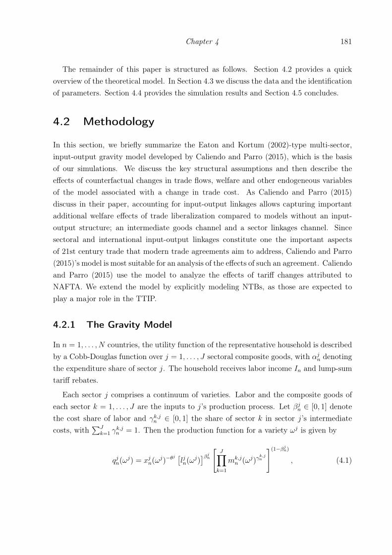
Chapter 4 181
The remainder of this paper is structured as follows. Section 4.2 provides a quickoverview of the theoretical model. In Section 4.3 we discuss the data and the identificationof parameters. Section 4.4 provides the simulation results and Section 4.5 concludes.
4.2 Methodology
In this section, we briefly summarize the Eaton and Kortum (2002)-type multi-sector,input-output gravity model developed by Caliendo and Parro (2015), which is the basisof our simulations. We discuss the key structural assumptions and then describe theeffects of counterfactual changes in trade flows, welfare and other endogeneous variablesof the model associated with a change in trade cost. As Caliendo and Parro (2015)discuss in their paper, accounting for input-output linkages allows capturing importantadditional welfare effects of trade liberalization compared to models without an input-output structure; an intermediate goods channel and a sector linkages channel. Sincesectoral and international input-output linkages constitute one the important aspectsof 21st century trade that modern trade agreements aim to address, Caliendo and Parro(2015)’s model is most suitable for an analysis of the effects of such an agreement. Caliendoand Parro (2015) use the model to analyze the effects of tariff changes attributed toNAFTA. We extend the model by explicitly modeling NTBs, as those are expected toplay a major role in the TTIP.
4.2.1 The Gravity Model
In n = 1, . . . , N countries, the utility function of the representative household is describedby a Cobb-Douglas function over j = 1, . . . , J sectoral composite goods, with αjn denotingthe expenditure share of sector j. The household receives labor income In and lump-sumtariff rebates.
Each sector j comprises a continuum of varieties. Labor and the composite goods ofeach sector k = 1, . . . , J are the inputs to j’s production process. Let βjn ∈ [0, 1] denotethe cost share of labor and γk,jn ∈ [0, 1] the share of sector k in sector j’s intermediatecosts, with
∑Jk=1 γ
k,jn = 1. Then the production function for a variety ωj is given by
qjn(ωj) = xjn(ωj)−θj [ljn(ωj)
]βjn [ J∏k=1
mk,jn (ωj)γ
k,jn
](1−βjn)
, (4.1)

182 Going Deep: The Trade and Welfare Effects of TTIP
where xjn(ωj) denotes the inverse efficiency of variety producer ωj. The dispersion of effi-ciencies across varieties is given by θj ∈ (0, 1). The higher θj, the greater the productivitydispersion in sector j. All varieties ωj are aggregated with a Dixit-Stiglitz-type CES tech-nology into sector j’s composite good. The sectoral composites are used for productionand consumption purposes.
A sector’s varieties are internationally traded and there is perfect competition amongvariety producers. Hence, prices equal marginal cost. Producers search across all countriesfor the lowest-cost supplier of a variety. When importing a variety from sector j in countryi, the importer n has to pay the unit costs cji times the trade costs κjin which consist of twoparts: ad-valorem tariffs τ jin ≥ 0 and iceberg trade costs djin ≥ 1, with djnn = 1. Followingother gravity applications, we model iceberg trade costs as a function of bilateral distance,PTAs, and other observable trade cost proxies such as a common border, a commonlanguage or a common colonial history. Accordingly, we assume djin = Din
ρj eδjZin , where
Din is bilateral distance, and Zin is a vector collecting dichotomous trade cost proxies.More explicitly, we allow for two types of PTAs: shallow and deep treaties. The respectivedummies are denoted by PTAshallow and PTAdeep. Since tariffs are an explicit part of tradecosts, the PTA dummies capture trade cost reductions that go beyond the reduction orelimination of tariffs. Thus, the PTA dummies capture the trade-enhancing effect ofreducing NTBs like sanitary and phytosanitary trade barriers and other technical barriersto trade like regulatory standards or labeling requirements.
The model gives rise to a gravity equation. Country n’s expenditure share πjin forsource country i’s goods in sector j depends on i’s price relative to the price index. It canbe written as
πjin =λji[cjiκ
jin
]−1
θj∑Ni=1 λ
ji
[cjiκ
jin
]−1
θj
. (4.2)
This trade share can be interpreted as the probability that, for country n, the lowest costsupplier of a variety in sector j is trade partner i. The model is closed with goods marketclearing and an income-equals-expenditure condition for each country n.
Besides “gross” trade flows, that is, the value of trade as measured at customs (towhich the trade shares in Equation (4.2) refer), we also consider trade in value added.Following Johnson and Noguera (2012b), we define value added exports as the amount ofvalue added from a source country absorbed (consumed or invested) in a foreign country.Johnson and Noguera (2012b) develop a methodology to compute bilateral sectoral valueadded trade flows based on trade data, value added shares in production, and internationalinput output tables. Aichele and Heiland (2015) (cp. Chapter 3 of this dissertation) showhow a structural equation for so-defined value added trade flows can be derived from
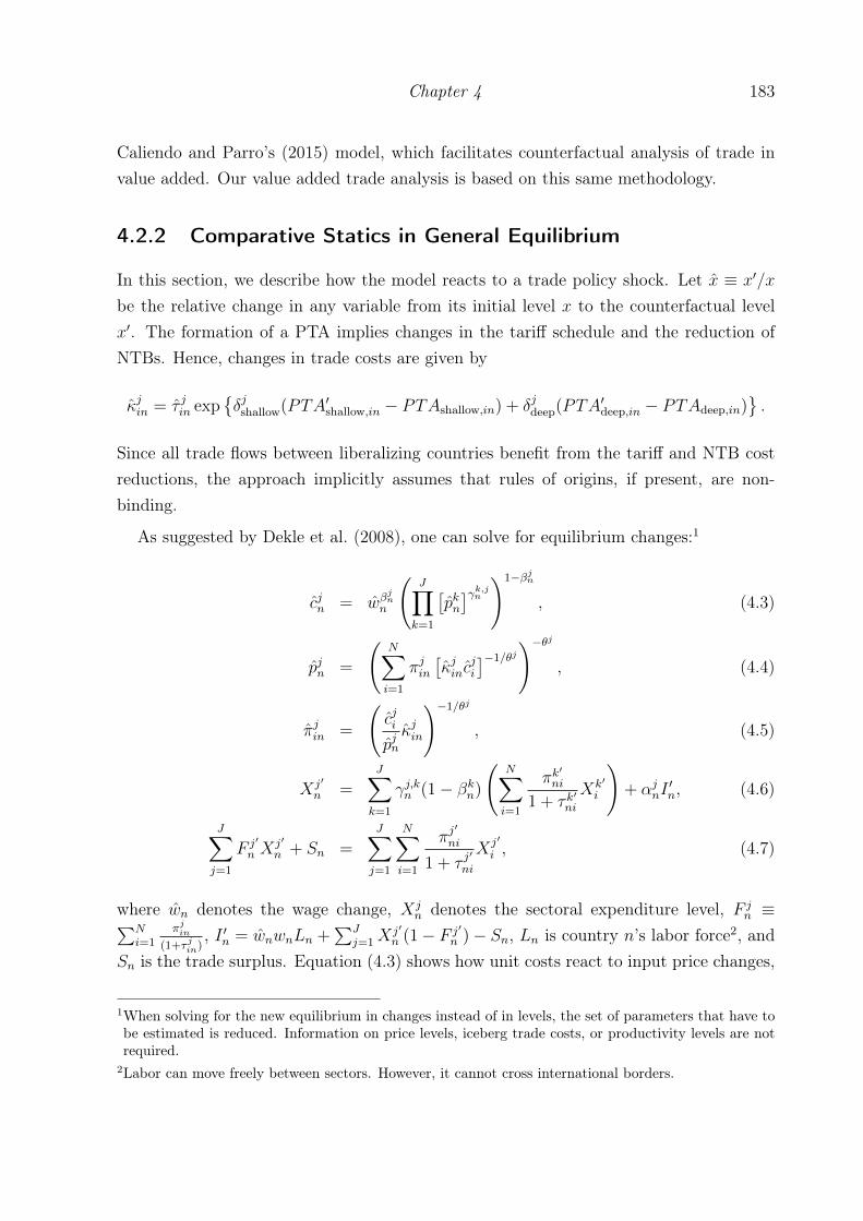
Chapter 4 183
Caliendo and Parro’s (2015) model, which facilitates counterfactual analysis of trade invalue added. Our value added trade analysis is based on this same methodology.
4.2.2 Comparative Statics in General Equilibrium
In this section, we describe how the model reacts to a trade policy shock. Let x ≡ x′/x
be the relative change in any variable from its initial level x to the counterfactual levelx′. The formation of a PTA implies changes in the tariff schedule and the reduction ofNTBs. Hence, changes in trade costs are given by
κjin = τ jin exp{δjshallow(PTA′shallow,in − PTAshallow,in) + δjdeep(PTA′deep,in − PTAdeep,in)
}.
Since all trade flows between liberalizing countries benefit from the tariff and NTB costreductions, the approach implicitly assumes that rules of origins, if present, are non-binding.
As suggested by Dekle et al. (2008), one can solve for equilibrium changes:1
cjn = wβjnn
(J∏k=1
[pkn]γk,jn )1−βjn
, (4.3)
pjn =
(N∑i=1
πjin[κjinc
ji
]−1/θj)−θj
, (4.4)
πjin =
(cjipjnκjin
)−1/θj
, (4.5)
Xj′n =
J∑k=1
γj,kn (1− βkn)
(N∑i=1
πk′ni
1 + τ k′
ni
Xk′i
)+ αjnI
′n, (4.6)
J∑j=1
F j′n X
j′n + Sn =
J∑j=1
N∑i=1
πj′ni
1 + τ j′ni
Xj′i , (4.7)
where wn denotes the wage change, Xjn denotes the sectoral expenditure level, F j
n ≡∑Ni=1
πjin(1+τ jin)
, I ′n = wnwnLn +∑J
j=1 Xj′n (1− F j′
n )− Sn, Ln is country n’s labor force2, andSn is the trade surplus. Equation (4.3) shows how unit costs react to input price changes,
1When solving for the new equilibrium in changes instead of in levels, the set of parameters that have tobe estimated is reduced. Information on price levels, iceberg trade costs, or productivity levels are notrequired.
2Labor can move freely between sectors. However, it cannot cross international borders.
184 Going Deep: The Trade and Welfare Effects of TTIP
i.e. to wage and intermediate price changes. Trade cost changes affect the sectoral priceindex pjn directly, and also indirectly by affecting unit costs (see Equation (4.4)). Changesin trade shares result from these trade cost, unit cost, and price changes. The strengthof the reaction is governed by the productivity dispersion θj. A small θj implies largetrade changes. Equation (4.6) ensures goods market clearing in the new equilibrium andEquation (4.7) corresponds to the counterfactual income-equals-expenditure or balancedtrade condition. The change in real income, which is given by
Wn =In
ΠJj=1(pjn)α
jn
, (4.8)
serves as our measure for the change in welfare.
Caliendo and Parro (2015) extend the single-sector solution algorithm proposed byAlvarez and Lucas (2007) to solve the system of equations given by (4.3)-(4.7). Thealgorithm starts with an initial guess of a vector of wage changes. With (4.3) and (4.4),it then computes price and trade share changes and the new expenditure levels based onthose wage changes, evaluates the trade balance condition (4.7), and then updates thewage change based on the error in the trade balance.
4.3 Data and Parameter Identification
To simulate the effects of the TTIP based on the model described in the previous section,we need to identify the parameters α, β, γ, θ, and δdeep and δshallow,3 and collect dataon bilateral trade shares π, tariff levels τ , countries’ total value added w · L, and tradesurpluses S. The expenditure shares α and the cost shares β and γ are obtained frominput-output tables. θ, δshallow and δdeep are estimated based on the gravity equationimplied by the model.
4.3.1 Data Sources
Our main data source is the Global Trade Analysis Project (GTAP) 9 database, whichprovides sectoral production values, sectoral value added information and bilateral finaland intermediate goods trade in producer and consumer prices, including service sectors.Based on this information, sectoral expenditures for final and intermediate goods, sectoral
3For the scenario considered later on this paper, we actually do not require estimates of δshallow. However,PTAshallow is certainly an important control variable in the estimation and will be needed if one definesthe scenario differently.

Chapter 4 185
bilateral tariffs, and bilateral input-output tables can be be constructed. The GTAPdatabase was chosen for its rich country detail.4 It contains data for 122 countries and18 aggregate regions (e.g. “Rest of Southeast Asia”). These 140 countries and regionsrepresent the world economy in the year 2011. GTAP distinguishes 57 sectors, which weaggregate to 38 following the sector groupings of GTAP in order to reduce the number ofparameters that need to be estimated.5
4.3.2 Expenditure and Cost Shares
Expenditure shares α, β, and γ, trade shares π, tariffs τ , and expenditure levels X areobtained from the GTAP database. We perfectly match final goods expenditure, sectoralbilateral trade flows (aggregating intermediate and final goods trade), and cost sharesfor intermediates and bilateral tariffs. Two adjustments to the data are necessary toalign it with the assumptions of the model. The first adjustment regards differences inbilateral trade shares between final and intermediate goods trade. The second adjustmentconcerns the international transport sector. In the model, the bilateral trade shares areassumed to be identical across use categories. In the GTAP data, however, bilateral tradeshares differ across final and intermediate usage. We match sectoral bilateral trade flows,final goods expenditure shares, and the cost shares for intermediates to their empiricalcounterparts and bilateralize final and intermediate goods trade with the common bilateraltrade share. Moreover, GTAP has a separate international transportation sector. Tomatch the iceberg trade cost assumption, we assign the international transport marginand its respective share of intermediate demand to the sectors demanding the internationaltransportation service. This increases the respective sector’s production value. Sectoralvalue added is then calculated as the difference between the so obtained production valuesand expenditures for intermediate goods, which also implies that we treat production taxesas part of domestic value added.
4.3.3 Identification of Trade Cost Parameters
A key element of our simulation is to distinguish shallow from deep PTAs and estimatetheir effect on bilateral NTBs. To that end, we classify existing PTAs as shallow or deep
4The World Input Output Database (WIOD) constitutes an alternative data source. It provides the sameinformation for a sample of 40 countries and the rest of the world for the years 1995-2011. Since we areinterested in trade creation and trade diversion and third country effects, we opted for GTAP in orderto maximize country coverage.
5An overview of the sectoral breakdown and the aggregation is provided in Table A4.11 in the appendix.

186 Going Deep: The Trade and Welfare Effects of TTIP
Figure 4.1: Status quo of depth of trade integration
0.1
.2.3
.4D
ensi
ty
0 1 2 3 4 5 6 7Depth index for PTAs
Note: The figure plots the index of depth of PTAs as classified by Dür et al. (2014) for country pairswith a PTA in 2011. The depth index counts the number of provisions and ranges from 0-7. Thedifferent provisions are: partial scope agreement, substantive provisions on services, investments,standards, public procurement, competition and intellectual property rights.
based on the number of provisions included in an agreement. Data on the number ofprovisions is obtained from the Design of Trade Agreements (DESTA) database (see Düret al., 2014). This database provides an index for the depth of PTAs, which is a countof the number of provisions (partial scope agreement, substantive provisions on services,investments, standards, public procurement, competition and intellectual property rights).The index ranges from 0 to 7, where 0 indicates a partial scope agreement and 7 is thedeepest level of integration. We recode this index of depth to obtain two classes of PTAs:shallow and deep agreements. The dummy indicating a shallow PTA switches to one ifthe depth index lies between 0 and 3. The dummy for a deep PTA takes the on valueone if the index lies between 4 and 7. Figure 4.1 shows the distribution of the depth ofexisting PTAs for the year 2011. About 16% of the PTAs (i.e., 2,522 bilateral relationsout of the 15,700 with a PTA in place) are classified as deep according to our definition;examples include NAFTA, the EU or USA-Korea agreement. The Andean Community,MERCOSUR or ASEAN are examples for shallow agreements.
The vectors of sectoral trade cost parameters θ, δdeep and δshallow can be identified fromthe gravity equation. Taking the trade share equation (4.2), plugging in the functional

Chapter 4 187
form for trade costs and multiplying by the total expenditure Xjn yields the following
log-linearized estimable gravity equation for each sector j:
ln(πjinXjn) = − 1
θjln τ jin −
ρj
θjlnDin −
δjshallowθj
PTAshallow,in −δjdeepθj
PTAdeep,in
− ζj
θjZin + νji + µjn + εjin, (4.9)
where νji ≡ ln(λjicji ) and µjn ≡ ln(Xj
n/∑N
i=1 λji
[cjiκ
jin
]−1
θj ) are importer and exporter fixedeffects, respectively, and εjin is an error term.
The coefficient on tariffs directly identifies the productivity dispersion, 1/θj. The higher1/θj, the stronger the response of trade flows to a cost shifter (here, bilateral tariffs).The coefficients of the PTA dummies, δdeep
j
θjand δshallow
j
θj, are expected to be positive,
since forming a PTA reduces non-tariff trade barriers, and thus increase bilateral trade.Naturally, we expect δdeep
j
θj> δshallow
j
θj. The change (in percent) in sectoral trade cost due
to a deep agreement for countries which previously did not have a shallow agreementimplied by the structural equation for trade cost is given by (eδ
jdeep−1)∗100. We estimate
Equation (4.9) sector by sector, thus allowing θj, δdeepj
θj, and δshallow
j
θjto be sector-specific.
The importer and exporter fixed effects take care of all, potentially unobserved, country-specific determinants of bilateral trade flows. However, the estimates of the PTA dummiesmight still suffer from an endogeneity bias if, for example, countries that trade more witheach other are also more likely to sign a PTA. In this case, the PTA dummy would over-estimate the trade enhancing effect of a PTA. To account for potential endogeneity, weuse an instrumental variables approach. A relevant and valid instrument influences theprobability to sign a PTA, but does not affect trade flows through any channel other thanthe PTA. Baldwin and Jaimovich (2012) propose a contagion index as an instrument.The contagion index rests on the idea that countries are more likely to form a PTA withpartners that already have many PTAs with third parties in place. Specifically, the indexmeasures the threat of trade diversion country i faces in a trade partner j’s market, bycounting j’s PTAs with third countries weighted with how important the third country’smarket is for i (i.e. with the third country’s share in i’s exports).6 We compute separatecontagion indices for shallow and deep PTAs.
Our estimations for the agricultural and manufacturing sectors are based on product-level (HS 6-digit) trade data from UN COMTRADE. The sample is restricted to the GTAPcountries. Data on bilateral tariffs for manufacturing sectors are taken from UNCTAD’s
6This instrument is, for example, also used by Martin et al. (2012).

188 Going Deep: The Trade and Welfare Effects of TTIP
TRAINS database. We use effectively applied tariffs including estimated ad-valoremequivalents of specific tariffs and quotas. We run separate regressions for our (partlyaggregated) GTAP sectors, using product fixed effects to absorb unobserved heterogeneity.Other trade cost proxies, i.e., bilateral distance and a dummy for contiguity, are obtainedfrom the CEPII distance database. We drop 0.5% of observations with the highest tariffsfrom the sample. Trade and tariff data are 5-year averages centered around 2011. For theservice sectors we use sector-level trade flows from the GTAP database.
Table 4.1 displays the IV gravity results for the productivity dispersion and the PTAeffects for the 4 agricultural and 18 manufacturing sectors. In general, our estimationscan explain between 25 and 55% of the variation in bilateral trade volumes. The coeffi-cients on tariffs satisfy the theoretical restriction 1/θj < −1 and are highly statisticallysignificant. Except for the “Mining (coal, oil and gas)” sector, where the number ofobservations is also quite small. The ranking of sectors in terms of their productivitydispersion seems sensible in most cases. Sectors like “Petroleum, coal products,” “Chemi-cal, rubber, plastic products,” or “Mining,” which produce fairly homogenous goods havea low θ, implying that trade flows react relatively strongly to cost changes. Sectors like“Wearing apparel,”“Electronic equipment,” or “Metal products,” on the other hand, havea relatively high θ which indicates that they provide more differentiated sectoral varieties.We find strong effects of deep PTAs on bilateral trade: Coefficients range between .16 inthe “Mineral products nec” industry and .9 in the “Motor vehicles and parts” industry.These estimates imply that deep PTAs increase trade by 17 to 145%, depending on thesector.7 We also find some evidence that shallow PTAs increase trade, at least in themanufacturing sectors. In other sectors, mostly the agricultural ones, the shallow PTAeffect is not statistically different from zero. For “Cattle, sheep, goats, horses” we actuallyfind a negative effect of shallow PTAs that is significant and in the Mining sector we findan implausible large effect of shallow PTAs. The coefficients on other trade cost proxies(as shown in Table (A4.12)) are as expected. Distance reduces bilateral trade volumes.A common border, common language and a shared colonial past tend to increase trade.
We also estimate the same specification with OLS. The resulting productivity dis-persion estimates and their ranking are fairly similar to the IV results, the PTA effectsobtained from OLS are smaller; see Table A4.14 in the Appendix. This result is well docu-mented in the literature; For example, Egger et al. (2011) also find that, counterintuitively,
7The trade-enhancing effect implied by a coefficient estimate of .16 is calculated as (e.16 − 1) ∗ 100.

Chapter 4 189
unobservable determinants of PTAs seem to be negatively correlated with bilateral tradevolumes. Consequently, OLS estimates of PTA dummies are downward biased.8
Table 4.2 provides IV gravity results for PTA effects in service sectors.9 In general,our specifications explain between 90 and 97% of the variation in bilateral service tradeflows. We find that both shallow and deep PTAs have large and significant effects on tradeflows. The magnitudes of the implied effects of deep agreements on trade range between13 and 79%, for the shallow agreements the range is 14 to 30%. Using OLS instead ofIV yields significantly smaller or insignificant effects for the PTA dummies, as shown inTable A4.15 in the Appendix. Since there are no tariffs levied on service trade, we cannotidentify θj in service industries. In the simulations, we use an average value from Eggeret al. (2012), who estimate a trade cost elasticity for services of 5.959. Moreover, we donot observe positive trade flows in the service industry “Dwellings;” hence, no PTA effectsare estimated for this sector. We set the change in trade cost in this sector to zero in thesimulations.
Remember that the structural interpretation of the coefficient for a deep PTA is − δdeepj
θj,
the combined effect of a deep PTA on non-tariff barriers and the effect of trade cost ontrade flows. With the estimated θs, we can thus back out the implied effect of PTAs ontrade cost. Figure 4.2 shows the reductions in NTBs implied by our IV estimates. Thegrey bars show equal-tailed 95% confidence intervals obtained by means of a bootstrapthat will be described in more detail below.
There is substantial heterogeneity across sectors: Trade cost reductions tend to belarger in manufacturing sectors, varying between 43% in the “Ferrous metals” industry and5% in “Machinery nec” and “Minerals.” In the agricultural sectors, we find significant tradecost reductions only for “Grains & Crops.” In the service sectors, trade cost reductionsrange between 4 and 9%, being largest in “Business services,” “Financial services,” and“Trade services.”
In our counterfactual analysis we assume that the TTIP will reduce the costs of non-tariff measures by the same amount that other PTAs have reduced trade barriers in thepast. Hence, we do not need to speculate about the changes in NTBs, and potentialsectoral heterogeneity therein, that may result from the implementation of the TTIP.
8For a brief survey on the size of existing PTA estimates in the literature see Felbermayr et al. (2015a).9Table A4.13 in the Appendix presents the complete results including the coefficient estimates for thecovariates. In stark contrast to goods flows, distance seems to be irrelevant as a trade cost indicator formost service sectors. A shared colonial past and a common border, on the other hand, strongly increasetrade in services.

190 Going Deep: The Trade and Welfare Effects of TTIP
Tab
le4.1:
IVgrav
ityestimates
man
ufacturing
sectors
(1)
(2)
(3)
(4)
(5)
(6)
(7)
(8)
(9)
(10)
Lntariff
Shallow
PTA
DeepPTA
Obs.
R2
Weak-ID
Und
er-ID
Sector
−1/θ
s.e.
−δ/θ
s.e.
−δ/θ
s.e.
F-stat
p-value
1Grains&
Crops
-2.310∗∗∗
0.148
0.249∗∗
0.106
0.401∗∗∗
0.118
243,624
0.29
346
0.00
2Cattle,
sheep,
goats,
horses
-2.441∗∗∗
0.163
-0.261∗∗
0.116
-0.204
0.125
90,274
0.34
458
0.00
3Fo
restry
-3.385∗∗∗
0.553
-0.024
0.156
0.086
0.150
22,304
0.32
347
0.00
4Fishing
-3.156∗∗∗
0.657
-0.182
0.210
0.076
0.209
28,274
0.30
148
0.00
5Mining(coal,oil,gas)
-6.021
4.199
1.269∗∗
0.591
0.830
0.542
6,669
0.41
980.00
6Mineralsnec
-3.695∗∗∗
0.690
0.357∗∗
0.144
0.364∗∗∗
0.129
85,350
0.25
244
0.00
7Livestock&
MeatProdu
cts
-2.498∗∗∗
0.093
0.188∗∗
0.082
0.289∗∗∗
0.091
531,429
0.30
471
0.00
8Textiles
-4.913∗∗∗
0.285
0.079
0.092
0.294∗∗∗
0.082
801,095
0.32
322
0.00
9Wearing
appa
rel
-1.613∗∗∗
0.398
-0.023
0.113
0.502∗∗∗
0.106
699,145
0.46
282
0.00
10Le
atherprod
ucts
-2.939∗∗∗
0.299
0.208∗∗
0.095
0.637∗∗∗
0.093
175,800
0.45
485
0.00
11Woo
dprod
ucts
-2.774∗∗∗
0.263
0.073
0.075
0.476∗∗∗
0.077
175,800
0.45
485
0.00
12Pap
erprod
ucts,p
ublishing
-4.697∗∗∗
0.241
0.146∗
0.079
0.526∗∗∗
0.078
223,734
0.45
672
0.00
13Petroleum
,coalp
rodu
cts
-5.463∗∗∗
1.220
0.807∗∗∗
0.186
0.672∗∗∗
0.205
317,824
0.42
636
0.00
14Chemical,rub
ber,plasticprod
s-4.743∗∗∗
0.218
0.201∗∗∗
0.071
0.317∗∗∗
0.072
22,745
0.39
480
0.00
15Mineral
prod
ucts
nec
-2.804∗∗∗
0.225
0.081
0.078
0.157∗∗
0.073
1,544,089
0.34
551
0.00
16Fe
rrou
smetals
-1.187∗∗∗
0.368
0.188∗
0.102
0.665∗∗∗
0.093
337,582
0.37
535
0.00
17Metalsnec
-3.691∗∗∗
0.452
0.611∗∗∗
0.121
0.752∗∗∗
0.102
302,429
0.32
355
0.00
18Metal
prod
ucts
-2.167∗∗∗
0.226
0.247∗∗∗
0.080
0.307∗∗∗
0.078
182,487
0.34
256
0.00
19Motor
vehicles
andpa
rts
-3.670∗∗∗
0.239
0.296∗∗∗
0.091
0.896∗∗∗
0.101
628,789
0.47
660
0.00
20Transpo
rtequipm
entnec
-2.315∗∗∗
0.287
0.136
0.089
0.409∗∗∗
0.086
157,463
0.54
650
0.00
21Electronicequipm
ent
-2.184∗∗∗
0.231
0.467∗∗∗
0.078
0.242∗∗∗
0.081
112,560
0.38
466
0.00
22Machinery
andequipm
entnec
-3.181∗∗∗
0.166
0.196∗∗∗
0.066
0.175∗∗∗
0.062
320,393
0.53
776
0.00
23Man
ufacturesnec
-2.275∗∗∗
0.204
0.169∗∗
0.077
0.251∗∗∗
0.076
2,212,282
0.46
720
0.00
Note:
The
tableshow
sgravityestimates
foragricultural
andman
ufacturing
sectorswithim
porter
andexpo
rter
dummiesan
dtheusua
lgravity
controls
(not
show
n).Stan
dard
errors
(inpa
rantheses)
arerobu
stto
clustering
oncoun
try-pa
irlevel.PTA
dummiesinstrumentedwithcontag
ion
indicesala
Martinet
al.(2012)or
Baldw
inan
dJa
imovich(2012)
fortherespective
depths.Sh
ea’sPartial
R2is0.19
forshallow
and0.23
fordeep
PTAs.
*,**
and***indicate
statisticals
ignifican
ceat
the10,5
and1%
level,respectively.

Chapter 4 191
Tab
le4.2:
IVgrav
ityestimates
servicesectors
(1)
(2)
(3)
(4)
(5)
(6)
(7)
(8)
Shallow
PTA
DeepPTA
Obs.
R2
Weak-ID
Und
er-ID
−δ/θ
s.e.
−δ/θ
s.e.
F-stat
p-value
25Gas
man
ufacture,d
istribution
0.141∗∗
0.062
0.389∗∗∗
0.089
13,546
0.97
877
0.00
26Water
0.229∗∗∗
0.031
0.377∗∗∗
0.053
11,368
0.95
673
0.00
27Con
struction
0.169∗∗∗
0.064
0.302∗∗∗
0.081
14,434
0.96
949
0.00
28Trade
0.129∗∗∗
0.037
0.580∗∗∗
0.056
14,518
0.90
927
0.00
29Transpo
rtnec
0.182∗∗∗
0.032
0.399∗∗∗
0.050
14,518
0.96
927
0.00
30Seatran
sport
0.024
0.055
0.413∗∗∗
0.075
14,518
0.95
927
0.00
31Airtran
sport
0.175∗∗∗
0.040
0.123∗∗
0.055
14,518
0.92
927
0.00
32Com
mun
ication
0.221∗∗∗
0.031
0.294∗∗∗
0.051
14,518
0.95
927
0.00
33Finan
cial
services
nec
0.160∗∗∗
0.040
0.490∗∗∗
0.060
14,518
0.95
927
0.00
34Insurance
0.152∗∗∗
0.033
0.338∗∗∗
0.054
14,518
0.95
927
0.00
35Businessservices
nec
0.267∗∗∗
0.035
0.559∗∗∗
0.054
14,518
0.96
927
0.00
36Recreationan
dotherservices
0.142∗∗∗
0.037
0.238∗∗∗
0.052
14,518
0.96
927
0.00
37Pub
Adm
in/D
efence/H
ealth/
Edu
cation
0.178∗∗∗
0.036
0.367∗∗∗
0.057
14,518
0.95
927
0.00
Note:
Allspecification
sinclud
eim
porter
andexpo
rter
fixed
effects
andtheusua
lgravity
controls(not
show
n).Stan
dard
errors
(inpa
renthe
ses)
areheteroskedasticity-rob
ustan
dclusteredat
thecoun
try-pa
irlevel.Sh
ea’s
Partial
R2is
0.11
4forshallow
and0.16
5fordeep
PTAs.
*,**
and
***indicate
statisticals
ignifican
ceat
the10,5
and1%
level,respectively.

192 Going Deep: The Trade and Welfare Effects of TTIP
Figure 4.2: Implied changes in NTBs-6
0-4
0-2
00
20C
hang
e in
NTB
s (in
%)
Gra
ins
& C
rops
Live
stoc
k fa
rmin
gFo
rest
ryFi
shin
gM
inin
gM
iner
als
nec
Mea
t Pro
duct
sTe
xtile
sW
earin
g ap
pare
lLe
athe
r pro
duct
sW
ood
prod
ucts
Pape
r pro
duct
sPe
trole
um, C
oal
Che
mic
als
Min
eral
sFe
rrous
met
als
Met
als
nec
Met
al p
rodu
cts
Mot
or v
ehic
les
Tran
spor
t equ
ipm
. nec
Elec
troni
csM
achi
nery
nec
Man
ufac
ture
s ne
cEl
ectri
city
Gas
Wat
erC
onst
ruct
ion
Trad
e se
rvic
esTr
ansp
ort n
ecSe
a tra
nspo
rtAi
r tra
nspo
rtC
omm
unic
atio
nFi
nanc
ial s
ervi
ces
Insu
ranc
eBu
sine
ss s
ervi
ces
Rec
reat
ion
Publ
ic s
ervi
ces
Dw
ellin
gs
equal-tailed 95% CI Mean
Note: The figure shows sectoral reductions in NTBs implied by the coefficient estimatesfrom the gravity equation (4.9) presented in Tables 4.1 and 4.2. (Equal-tailed) confidenceintervals are computed based on 425 bootstrap replications using Hall (1992)’s percentilemethod.
Moreover, we acknowledge in our simulation the fact that the trade cost changes and thesectoral productivity dispersion parameters are estimated. Uncertainty about parameterestimates θ, δshallow, δdeep derives from the fact, that the dataset based on which theyare estimated is itself just a random draw of the underlying data generating processcharacterized by the true values of θ0,ρ0shallow,ρ0deep. The trade cost changes displayedin Figure 4.2, and, in fact, all outcomes of our simulation, are more or less complicatedfunctions of the estimated parameters and hence, they are random variables as well. Toobtain measures of uncertainty, that is, confidence intervals, for the model outcomes, webootstrap an empirical distribution of the θ, δshallow, δdeep. That is, we draw 425 bootstrapsamples (independently for every sector), estimate θb, δb,shallow, δb,deep and collect the 425

Chapter 4 193
sets of estimates.10 For every set of parameters b = 1, ..., 425, we then simulate theeffects of the TTIP and collect the variables of interest, such as changes in trade flows,output, and welfare. Thereby, we obtain a distribution of every model outcome reflectingthe uncertainty present in our estimation stage, or, in fact, the uncertainty present inthe data. Throughout the analysis, we calculate confidence intervals according to thepercentile method proposed by Hall (1992).11
4.4 Simulation Results: Trade and Welfare Effects ofthe TTIP
We now have paved the way to simulate the effect of the TTIP. Our scenario of a “deepTTIP” assumes that NTBs to trade between EU countries and the United States fall bythe amount estimated in the previous section and that all tariffs between the EU andthe United States are set to zero. A slight complication regarding the calibration of themodel based on data from 2011 is caused by Croatia’s entry into EU in July 2013. In our2011 data, Croatia is not yet an EU member, however, it will be part of the TTIP. Inorder not to confound the effects of the TTIP with the effects of Croatia’s EU accession,we simulate a counterfactual baseline equilibrium describing the world in 2011 if Croatiahad been a member already at that time.12 Based on this counterfactual equilibrium, wethen evaluate the effects of the TTIP. Except for Croatia and its neighboring countries,the change from the 2011 equilibrium to the counterfactual baseline with Croatia in theEU has negligible effects on the status quo of the countries in our analysis.13
We start our discussion of the effects of the TTIP with a summary of the status quo.Then, we present the simulation results, starting with the effects on global and bilateraltrade in terms of gross flow and value added and analyze the role globally fragmented valuechains in spreading the TTIP’s effects across the globe. Next, we discuss how sectoralvalue added is affected in different parts of the world. Finally, we investigate the regionaland global welfare changes that the TTIP would bring about.
10Since we expect standard errors to be correlated within country pairs, we conduct a block bootstrapwithin each sector, drawing country pairs instead of individual observations.
11Hall’s percentile method uses the quantiles of the bootstrapped distribution of the θ − θb rather thanjust the quantiles θb to form confidence bounds, which ensures that the coverage probability is correctlycaptured if the distribution of the original estimate θ is asymmetric.
122011 is the most recent year for which input-output data for the 140 countries/regions is available. Wedo not predict baseline values for some future year, as Fontagne et al. (2013) or Francois et al. (2013),since this would introduce additional margins of error.
13Details are available from the authors upon request.

194 Going Deep: The Trade and Welfare Effects of TTIP
4.4.1 Cross-industry facts for the EU and the United States
Tables 4.3 and 4.4 provide information on the status quo of trade between the EU and theUnited States. All values are in US dollars and relate to the base year of 2011 includingthe model-based predicted adjustments for Croatia’s EU entry. Column (1) of Table4.3 reports, by sector, the value added generated in the EU. 72% of total value added(GDP) is generated in the service sectors, 25% in manufacturing, and 2% in agriculture.Columns (2) and (5) show that total EU exports to the United States amount to 521 bn.US dollars which equals about 8% of total exports (excluding trade among EU countries).However, in value added terms, exports of 448 bn. US dollars to the United States accountfor more than 10% of the total.14 This signals that EU exports to the United Statesincorporate relatively little reexports of foreign value added (including value added thatwas previously imported from the United States in the form of intermediates). Column(4) provides trade-weighted sector-level tariff rates that EU exporters face in the UnitedStates. These tariffs are low; the trade-weighted average rate (excluding services trade) isjust 1.3%. Exports to the world (Column 7) encounter very similar tariff rates; thus, earlierrounds of (multilateral) trade liberalization have not particularly favored EU exports tothe United States. Columns (5) and (6) report EU exports to the world. The comparisonwith Columns (2) and (3) shows that the United States is a particularly important marketfor EU services exporters: In the majority of service sectors the share of total exportsgoing to the United States exceeds the 10% average (in VA terms) by a wide margin. Theopposite is true in the agri-food sectors. The share of exports from manufacturing sectorsgoing to the United States is also below the 10% average in most case.
Table 4.4 provides similar descriptive statistics for the United States. It shows thatservices industries in the United States account for an even larger share in total valueadded than in the EU (82%). The share of the agri-food sectors in total value addedis comparable to the EU (2%). The United States is slightly smaller in terms of GDP(15,257 bn. vs. 16,186 bn.) and less open; domestic value added embodied in foreignabsorption relative to domestic GDP amounts to 9%; in the EU the ratio equals 27%. TheEU has a bilateral surplus with the United States of 31 bn. USD in gross terms and of62 bn. USD in value added terms. This signals that a lot of EU value added reaches theUnited States via third countries. Moreover, exports to the EU are much more importantfor the United States (26% of total) than exports to the United States are for the EU(10%). Average tariffs faced by US exporters in the EU are slightly larger than vice versa.The correlation between the two tariff schedules across sectors is relatively high (.3).
14Value added exports to the EU reflect European value added embodied in US.

Chapter 4 195
Table 4.3: Status quo summary statistics: EU28
(1) (2) (3) (4) (5) (6) (7)Sector Value Exports to U.S. Exports to World∗
added Gross VA Tariffs Gross VA Tariffs(in bn. USD) (in %) (in bn. USD) (in %)
Grains & Crops 172 1 3 2.97 99 75 0.68Cattle, sheep, goats, horses 169 1 2 1.20 85 49 1.18Forestry 32 0 1 0.48 6 17 0.26Fishing 17 0 0 0.36 8 6 0.06Mining (coal, oil, gas) 83 1 5 0.10 33 50 0.05Minerals nec 45 0 3 0.04 42 29 0.02Livestock & Meat Products 495 20 11 2.51 336 153 2.19Textiles 92 4 3 5.96 98 48 6.98Wearing apparel 93 3 1 10.32 71 32 10.37Leather products 47 3 2 7.30 54 25 12.40Wood products 89 4 4 0.34 103 50 0.36Paper products, publishing 284 5 9 0.01 154 115 0.00Petroleum, coal products 258 16 13 1.61 189 121 0.85Chemical, rubber, plastic prods 600 100 54 1.33 1,059 440 1.18Mineral products nec 149 5 4 4.11 80 54 2.93Ferrous metals 112 8 7 0.19 193 84 0.21Metals nec 68 8 5 1.73 173 56 0.53Metal products 285 7 13 1.77 169 146 1.57Motor vehicles and parts 289 42 16 1.15 676 194 0.56Transport equipment nec 106 24 9 0.12 184 64 0.46Electronic equipment 143 10 7 0.30 242 92 0.18Machinery and equipment nec 701 89 49 0.86 1,043 452 0.79Manufactures nec 133 14 6 0.92 92 46 1.03Electricity 294 0 8 0.00 35 95 0.00Gas manufacture, distribution 21 0 0 0.00 3 6 0.00Water 45 0 1 0.00 1 8 0.00Construction 1,053 1 4 0.00 53 62 0.00Trade services 1,123 7 15 0.00 162 158 0.00Transport nec 516 17 20 0.00 139 181 0.00Sea transport 32 1 2 0.00 66 24 0.00Air transport 84 19 8 0.00 141 53 0.00Communication 387 5 12 0.00 62 103 0.00Financial services nec 570 25 25 0.00 144 163 0.00Insurance 155 25 11 0.00 74 40 0.00Business services nec 2,421 31 85 0.00 493 830 0.00Recreation and other services 535 6 8 0.00 87 93 0.00PubAdmin/Defence/Health/Education 3,359 19 21 0.00 95 138 0.00Dwellings 1,127 0 0 0.00 0 2 0.00Total 16,186 521 448 1.33 6,744 4,351 1.37
Note: The table shows aggregate sectoral value added, exports and value added exports to the UnitedStates and the world in the baseline equilibrium (2011 with Croatia in the EU), and the respective tariffsfor the EU28; Average tariffs in the last row reflect trade-weighted averages of tariffs in manufacturingand agriculture. ∗ EU exports to World exclude intra-EU trade.

196 Going Deep: The Trade and Welfare Effects of TTIP
Table 4.4: Status quo summary statistics: United States
(1) (2) (3) (4) (5) (6) (7)Sector Value Exports to EU28 Exports to World
added Gross VA Tariffs Gross VA Tariffs(in bn. USD) (in %) (in bn. USD) (in %)
Grains & Crops 130 6 5 3.38 91 52 2.61Cattle, sheep, goats, horses 84 1 1 23.78 25 11 27.89Forestry 13 0 0 1.12 3 2 0.23Fishing 5 0 0 7.86 1 1 2.76Mining (coal, oil, gas) 229 6 21 0.00 19 72 0.00Minerals nec 29 2 3 0.02 12 11 0.01Livestock & Meat Products 230 6 4 11.09 58 26 7.73Textiles 62 2 2 6.01 17 10 5.32Wearing apparel 32 1 0 10.42 4 1 7.28Leather products 6 1 0 3.68 3 1 7.39Wood products 121 2 2 0.98 13 10 0.66Paper products, publishing 245 6 9 0.02 40 40 0.01Petroleum, coal products 42 35 4 1.78 137 13 0.51Chemical, rubber, plastic prods 422 75 40 2.13 282 151 1.57Mineral products nec 77 3 3 3.08 14 13 3.06Ferrous metals 75 2 5 0.42 30 25 0.18Metals nec 45 15 6 1.92 52 21 0.88Metal products 167 6 7 2.08 34 35 1.69Motor vehicles and parts 143 12 4 7.88 120 29 4.26Transport equipment nec 117 34 16 1.17 93 46 1.27Electronic equipment 77 18 5 0.56 97 20 0.94Machinery and equipment nec 536 63 37 1.29 314 172 1.19Manufactures nec 48 8 4 .91 25 11 1.20Electricity 195 0 5 0.00 1 18 0.00Gas manufacture, distribution 37 1 1 0.00 2 4 0.00Water 68 0 1 0.00 1 5 0.00Construction 923 2 6 0.00 8 24 0.00Trade services 1,971 7 30 0.00 21 122 0.00Transport nec 289 20 16 0.00 38 49 0.00Sea transport 32 1 1 0.00 2 5 0.00Air transport 86 15 6 0.00 34 17 0.00Communication 326 7 7 0.00 14 21 0.00Financial services nec 1,172 33 35 0.00 57 96 0.00Insurance 322 6 5 0.00 21 20 0.00Business services nec 1,534 60 69 0.00 115 202 0.00Recreation and other services 501 12 7 0.00 35 21 0.00PubAdmin/Defence/Health/Education 3,501 23 20 0.00 79 69 0.00Dwellings 1,367 0 0 0.00 0 0 0.00Total 15,257 490 386 2.17 1,912 1,448 1.87
Note: The table shows the United States’ sectoral value added, exports and value added exports to theEU28 and the world in the benchmark equilibrium (2011 with Croatia in the EU), and the respective tariffs.Average tariffs in the last row reflect trade-weighted averages of tariffs in manufacturing and agriculture.

Chapter 4 197
Table 4.5: Global trade effects of the TTIP by broad sector
Initial Exports Growth Initial share Change in share(in bn. USD) (in %) 95% CI (in %) (in %pts.) 95% CI
Agriculture 725 0.38 [0.10, 0.63] 3.60 -0.06 [-0.08, -0.05]Manufacturing 16,079 1.71 [1.32, 1.93] 79.77 -0.40 [-0.56, -0.23]Services 3,352 5.06 [3.84, 6.08] 16.63 0.46 [0.29, 0.63]
Total 20,157 2.22 [1.82, 2.45] 100 0.00 -
Note: Exports valued in fob-terms. (Equal-tailed) confidence intervals are computed based on 425bootstrap replications using Hall (1992)’s percentile method.
4.4.2 Global Trade Effects of the TTIP
Reflecting the official ambitions for the TTIP, our counterfactual scenario assumes that alltransatlantic tariffs are eliminated. Moreover, we assume that NTBs between the UnitedStates and the EU are reduced by the same amount as in existing deep PTAs. Table 4.5presents the changes in aggregate trade patterns implied by the model. World trade ispredicted to increase by about 2.2%.15 The model also predicts that the TTIP affectsthe sectoral composition of aggregate trade flows. The strongest trade growth occurs inthe service sector, where the predicted increase is 5%. This increases the share of servicetrade in total trade, which was initially at 17%, by .5 percentage points, at the expenseof the shares of manufacturing and agricultural goods. However, trade in manufacturingand agriculture also increases in absolute terms, by 1.7 and .4%, respectively. Irrespectiveof the considerable amount of uncertainty around the precise trade cost reduction impliedby the data as visualized in Figure 4.2, the changes in trade aggregate patterns predictedby the model are all significantly different from zero.
The predicted growth in gross trade, however, is not indicative of the growth in worldGDP (or value added) induced by the TTIP. Trade in intermediates – which are used toproduce traded goods in consecutive stages of production and might thus cross bordersmultiple times – drives a wedge between the trade volume registered at customs and thevalue added content of countries’ exports. More specifically, trade in intermediate goodsleads to double counting of value added from upstream stages of production. Table 4.6shows that in the baseline equilibrium value added worth 14.4 tn. US dollars (10% ofworld GDP) was exported, that is, absorbed (consumed or invested) in a country otherthan the country of origin. Comparing this number to the recorded trade volume of 20.2tn. US dollars (Column (1) in Table 4.5), we find a value added export to export (VAX)
15Note that intra-regional trade in GTAP’s “Rest of ...” regions is not included in this number.

198 Going Deep: The Trade and Welfare Effects of TTIP
Table 4.6: Global value added trade effects of the TTIP by broad sector
Value added exports VAX ratioInitial Share Growth w. TTIP Initial With TTIP
(in bn. USD) (in %) (in %) (in %) (in %)Agriculture 746 5.2 0.2 102.9 102.7Manufacturing 8,246 57.4 1.3 51.3 51.1Services 5,374 37.4 2.8 160.3 156.8Total 14,366 100.0 1.8 71.3 71.0
ratio of 71.3%. Thus, almost 30% of the trade volume measured at customs is double-counted value added. With the TTIP, our model predicts value added trade to increaseby 1.8%.16 Hence, growth in world value added trade induced by the TTIP falls behindgrowth in world gross exports; the VAX ratio declines slightly. Presumably, the TTIPincreases the extent of double-counting of value added in trade statistics, because it leadsto more back-and-forth trade of intermediates among the TTIP countries.
Decomposing total value added trade into manufacturing, services and agriculturalvalue added reveals that services trade is more important than recorded trade flows wouldsuggest. Even though manufacturing value added accounts for the largest part of exportedvalue added (57%), its share is much smaller than the share in recorded trade flows (80%).The VAX ratio of manufacturing is only 51%, indicating that manufacturing trade partlytakes place in the form of intermediates trade and that traded manufacturing goodsembody a significant amount of value added from the services industries. Indeed, whilethe recorded services trade is about 3.4 bn. USD, the value added from the servicessectors embodied in global trade amounts to 5.4 bn. USD. Services thus account for 37%of exported value added, but only for 17% of recorded trade volumes. Accordingly, theVAX ratio for services is very large (160%). Under the TTIP, agricultural, manufacturingand services value added trade all grow, but, especially in the case of services, at a muchsmaller rate than gross trade flows.
4.4.3 Bilateral Trade Effects of the TTIP
Table 4.7 looks into the TTIP’s effects on regional trade relationships. Again, we discusschanges in gross trade and trade in value added. Our model predicts a substantial amountof trade creation between the EU and the United States in the long run. EU exports tothe United States are expected to increase by 55%, US exports to the EU would go up
16We do not compute confidence intervals for the value added trade flows because the computationalburden is enormous. The computation of value added exports involves inverting a (140×38)×(140×38)matrix, which would have to be conducted for every bootstrap sample.

Chapter 4 199
Table 4.7: Aggregate trade effects of the TTIP
(1) (2) (3) (4) (5) (6) (7) (8) (9)Region ASEANb Brazil Canada China EU28 Mexico SACUa Turkey USAExport growth (in %) from ... toASEAN -0.3 -0.3 -0.7 -0.5 -0.2 -0.9 -0.6 -0.5 -0.7Brazil -0.3 -0.3 -2.0 -0.5 -0.3 -1.9 -0.7 -0.6 -0.5Canada -0.0 -0.1 -0.4 -0.3 -3.8 -1.2 -0.3 -0.4 -1.3China -0.3 -0.2 -0.6 -0.4 -0.2 -0.7 -0.4 -0.4 -1.0EU28 -0.7 -0.7 -1.3 -0.7 -0.4 -1.4 -0.8 -0.8 54.5Mexico 0.4 0.3 -1.3 0.2 -0.9 -0.6 -0.0 -0.2 -1.5SACU -0.3 -0.1 -1.4 -0.3 -0.4 -0.6 -0.4 -0.6 -2.6Turkey -0.2 -0.2 -1.6 -0.4 -0.3 -1.3 -0.4 -0.3 -1.2USA -1.1 -1.0 -1.6 -1.0 58.5 -1.4 -1.1 4.9 -0.5Growth of value added transfers (in %) from ... toASEAN -0.3 -0.4 -0.1 -0.2 -1.2 0.3 -0.3 -0.4 0.2Brazil -0.4 -0.3 0.2 -0.2 -1.3 0.6 -0.3 -0.5 0.4Canada -0.6 -0.8 -0.3 -0.5 2.1 -0.7 -0.6 -0.2 -1.7China -0.5 -0.5 -0.4 -0.3 -1.2 0.3 -0.3 -0.6 0.4EU28 -0.6 -0.4 4.8 -0.2 -0.4 11.9 -1.7 -1.1 46.9Mexico -1.0 -1.0 -1.3 -0.8 3.9 -0.5 -0.7 -0.2 -2.2SACU -0.6 -0.6 -0.0 -0.4 -1.8 0.9 -0.3 -0.9 3.5Turkey -0.6 -0.5 1.5 -0.4 -1.7 3.7 -0.6 -0.3 8.0USA 0.0 -0.1 -1.8 -0.6 40.5 -1.7 0.4 5.2 -0.3
Note: Diagonals describes changes in intra-national trade and/or in the trade volume withina region. a Southern African Customs Union, b Association of Southeast Asian Nations.
by 59%. However, trade statistics exaggerate the actual transfer of value added betweenthe two transatlantic regions. EU value added exports to the United States are predictedto increase only by 47%, US value added exports increase by 41% under the TTIP. Thisimplies that the VAX ratio of EU exports to the United States declines from 86% (asimplied by the last row of Table 4.3) to 78%. Similarly, the VAX ratio of US exports tothe EU declines from 79 to 61%. This suggests that the TTIP leads to a deepening oftransatlantic production chains. Intensified intermediate goods trade between the EU andthe United States will lead to a higher foreign value added content of production, increasethe extent of double-counting as well as the value added from either of the two partnersthat is processed by the other and sold to third parties. All these factors contribute tothe wedge between recorded trade volumes and actual value added transfers.
The fact that the TTIP countries engage in global production sharing along the valuechain implies that the economic consequences of trade diversion are only partially capturedby changes in the pattern of bilateral trade flows with non-TTIP countries. Table 4.7shows that the EU and the United States are predicted to export less to and import lessfrom non-TTIP countries. In value added terms, however, the picture is more nuanced. Inparticular, the predicted patterns show how the growing transatlantic production networkinteracts with the existing North American and European production network. Eventhough the EU exports less to Canada (-1.3%), Canadian absorption of European value

200 Going Deep: The Trade and Welfare Effects of TTIP
added increases by 4.8%. We find a similar pattern for the EU’s trade with Mexico. Thispattern emerges because, with the TTIP, relatively more value added from the EU entersproduction in the United States embodied in intermediates, that will then be absorbedin Canada and Mexico who trade intensively with the United States. Vice versa, the EUabsorbs more Canadian and Mexican value added, which reaches the EU embodied inUS exports. Canadian value added exports to the EU increase by 2.1%; compared to adecrease in Canadian exports of -3.8%.
The EU, on the other hand, has production networks, for example, with Turkey andSouth Africa. Even though exports from the Southern African Customs Union to theUnited States fall by 2.6%, the SACU value added exports to the United States increaseby 3.5%. Another interesting case is the United States’United States trade relationshipwith Turkey. Turkey is in a customs union with the EU, and so the Turkish import tariffson US products would also be eliminated under the TTIP. Thus, US exports to Turkeyare stimulated and increase by 4.9%. The asymmetric nature of the Turkish currencyunion with the EU becomes evident when looking at Turkey’s exports to the UnitedStates. The United States does not eliminate its import tariffs on Turkish products withthe TTIP, and hence, Turkish exporters suffer from trade diversion on the US market.Turkish exports to the United States fall by 1.2%. But indirectly (presumably due tostrong input-output linkages with the EU), Turkish value added exports to the UnitedStates still grow by 8%.
Table 4.7 also shows that the TTIP will lead to trade diversion within the EU. Intra-EUtrade both in gross terms and in terms of value added falls by .4%. The TTIP tends toreduce trade flows between third countries. But in some cases, it stimulates trade amongthird countries, such as, for example, Mexico’s export to Brazil, China, and the ASEANcountries are expected to increase. This ambiguity is due to three potentially opposingeffects: first, income in third countries can rise or fall and thus impact imports througha general demand effect; second, trade may rise as exports that went to the EU or theUnited States in the baseline situation are redirected; and third, wage increases in theTTIP countries enhance the relative competitiveness of other exporters in third markets.
Summarizing, trade and value added trade changes mostly follow similar patterns.However, there are some important exceptions where recorded and value added tradeflows change disproportionately or even go in different directions. This is the result ofnewly forming or existing international production chains. These findings highlight thatusing a model with input-output relationship that can capture the interconnectednessof countries and sectors in the global value chain is vital for an analysis of structuraleconomic changes such as the integration of regional markets.
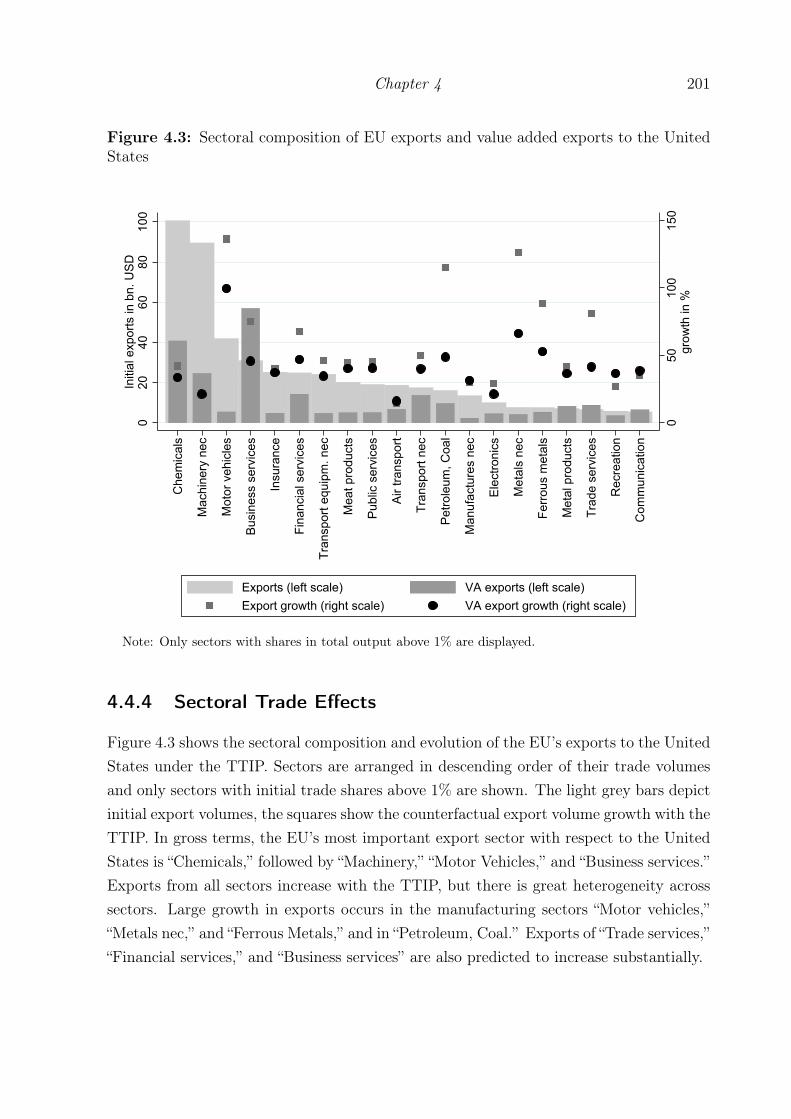
Chapter 4 201
Figure 4.3: Sectoral composition of EU exports and value added exports to the UnitedStates
050
100
150
grow
th in
%
020
4060
8010
0In
itial
exp
orts
in b
n. U
SD
Che
mic
als
Mac
hine
ry n
ec
Mot
or v
ehic
les
Busi
ness
ser
vice
s
Insu
ranc
e
Fina
ncia
l ser
vice
s
Tran
spor
t equ
ipm
. nec
Mea
t pro
duct
s
Publ
ic s
ervi
ces
Air t
rans
port
Tran
spor
t nec
Petro
leum
, Coa
l
Man
ufac
ture
s ne
c
Elec
troni
cs
Met
als
nec
Ferro
us m
etal
s
Met
al p
rodu
cts
Trad
e se
rvic
es
Rec
reat
ion
Com
mun
icat
ion
Exports (left scale) VA exports (left scale)Export growth (right scale) VA export growth (right scale)
Note: Only sectors with shares in total output above 1% are displayed.
4.4.4 Sectoral Trade Effects
Figure 4.3 shows the sectoral composition and evolution of the EU’s exports to the UnitedStates under the TTIP. Sectors are arranged in descending order of their trade volumesand only sectors with initial trade shares above 1% are shown. The light grey bars depictinitial export volumes, the squares show the counterfactual export volume growth with theTTIP. In gross terms, the EU’s most important export sector with respect to the UnitedStates is “Chemicals,” followed by “Machinery,” “Motor Vehicles,” and “Business services.”Exports from all sectors increase with the TTIP, but there is great heterogeneity acrosssectors. Large growth in exports occurs in the manufacturing sectors “Motor vehicles,”“Metals nec,” and “Ferrous Metals,” and in “Petroleum, Coal.” Exports of “Trade services,”“Financial services,” and “Business services” are also predicted to increase substantially.

202 Going Deep: The Trade and Welfare Effects of TTIP
Figure 4.4: Sectoral composition of US exports and value added exports to the EU
050
100
150
200
250
grow
th in
%
020
4060
80In
itial
exp
orts
in b
n. U
SD
Che
mic
als
Mac
hine
ry n
ec
Busi
ness
ser
vice
s
Petro
leum
, Coa
l
Tran
spor
t equ
ipm
. nec
Fina
ncia
l ser
vice
s
Publ
ic s
ervi
ces
Tran
spor
t nec
Elec
troni
cs
Met
als
nec
Air t
rans
port
Mot
or v
ehic
les
Rec
reat
ion
Man
ufac
ture
s ne
c
Com
mun
icat
ion
Trad
e se
rvic
es
Insu
ranc
e
Mea
t pro
duct
s
Met
al p
rodu
cts
Gra
ins
& C
rops
Min
ing
Pape
r pro
duct
s
Exports (left scale) VA exports (left scale)Export growth (right scale) VA export growth (right scale)
Note: Only sectors with shares in total output above 1% are displayed.
Figure 4.3 also shows the EU’s sectoral value added exports to the United States in theinitial situation (dark grey bar) and the counterfactual growth with the TTIP (black dot).Interestingly, in value added terms, the EU’s top export sector is no longer “Chemicals,”but rather “Business services.” As discussed earlier, a lot of service value added is tradedindirectly, embodied in the exports and imports of tradable goods. Accordingly, growthin value added exports is significantly smaller compared to growth in gross exports in themanufacturing sectors. In the service sectors the two are commensurate. Nevertheless,the manufacturing sectors “Motor vehicles,” “Metals nec,” and “Ferrous Metals,” as wellas “Petroleum, Coal” experience the highest growth rates also in valued added terms.
Figure 4.4 shows a similar graph for US exports to the EU. As for the EU, “Chemicals”is the United States’ most important export sector in gross terms, but “Business services”account for the largest part of US value added absorbed in the EU. Export growth is pre-dicted to be extremely large in the “Motor vehicles” sector (250%). Moreover, US exports

Chapter 4 203
are predicted to increase substantially in “Metals nec,” “Mining,” “Petroleum, Coal,”“Meatproducts,” “Trade services,” and “Grains & Crops.” These sectors also experience thelargest growth rates in terms of value added exports.
4.4.5 Effects on Sectoral Value Added
In this section, we investigate the effects of the TTIP on the sectoral production structure.Table 4.8 shows, by region, the share of agriculture, manufacturing and services in totalvalue added, the predicted change in value added due to the TTIP, and the predictedchange in the aggregate sector’s share in total value added of the region. Both in theEU and the United States, service industries make up by far the largest part of totalvalue added (73% in the EU and 81% in the United States). Manufacturing is thus moreimportant in the EU than in the United States. In Germany, for example, the share ofmanufacturing is 26.2% and higher than in most developed economies. Agricultural valueadded plays a minor role for both TTIP countries. Our simulations predict that the TTIPleads to a slight reindustrialization in the EU. The share of manufacturing value addedin total value added increases by 0.1 percentage points, on average. Service industriesand agriculture lose a small share in total value added. In the United States, the sectoraloutput structure changes very little.
Table 4.8 also shows that the TTIP leads to deindustrialization in the non-TTIP coun-tries. The share of services in total value added tends to increases to the detrimentof manufacturing in all non-TTIP regions with the exception of the countries in theAlianza del Pacifico, who experience a shift away from the manufacturing and servicestowards agriculture, and a few non-TTIP European countries, where both agricultureand manufacturing gain significant output shares. This pattern of deindustrializationversus reindustrialization is also supported by Figure 4.5, which shows distributions ofthe changes in sectoral shares (manufacturing and services only) across countries, fornon-TTIP and TTIP members. The distribution of changes in manufacturing shares fornon-TTIP countries (dark grey dashed line) lies to the left of the respective distributionof changes among the TTIP countries (dark grey solid line) and reaches much further intothe negative range. The opposite pattern is obtained for the distribution of changes inthe service sectors which tend to be positive for the non-TTIP countries (light grey lines).
Within the EU, however, the reindustrialization trend is not universal. Table 4.8 laysout the sectoral changes for the 28 EU countries. The shift towards manufacturing isdriven primarily by the Western European economies; Austria, Germany, Belgium, Ire-land, Finland, Great Britain, and Sweden. Some Central and Eastern European economies

204 Going Deep: The Trade and Welfare Effects of TTIP
Figure 4.5: Changes in manufacturing and services shares with the TTIP0
510
15D
ensi
ty
-1 -.5 0 .5 1Change in sector shares in total value added (in %pts.)
TTIP countries: Non-TTIP countries:Manufacturing ManufacturingServices Services
kernel = epanechnikov, bandwidth = 0.0577
Note: The figure shows the density of changes of the share of manufacturing (black lines) and services(grey lines) value added (in percentage points) for the TTIP scenario of deep trade integrationdistinguished by the TTIP (solid lines) and non-TTIP countries (dashed lines).
like Bulgaria, Cyprus, Slovenia as well as Luxembourg shift production away from man-ufacturing towards services and, in the case of Bulgaria, towards agriculture.
On the more disagreggated level, sectoral effects are very heterogeneous across coun-tries. Figure 4.6 plots sectoral value added changes for four exemplary countries, theUnited States, Germany, Canada, and Japan. In every panel, sectors are ordered by theirinitial shares in total value added of the respective countries, with shares decreasing fromleft to right. In the United States (upper left panel) all important sectors except for theinsurance industry gain. “Mining” value added is predicted to increase strongly, howevernot significantly so. The large margin of error owes to the fact, that the effect of deeptrade agreements on changes in this sector are estimated with low precision (cp. Table4.1). Germany experiences a huge value added increase in the “Motor vehicles” sector andsignificant gains in “Metal products,” but also small losses in important sectors such as“Transport (equipment) nec” and “Financial services.”

Chapter 4 205
Tab
le4.8:
The
effects
oftheTTIP
onsectoral
valuead
ded,
byregion
Agr
icult
ure
Man
ufa
cturi
ng
Ser
vice
sCha
nge
Cha
nge
Cha
nge
Cha
nge
Cha
nge
Cha
nge
Initials
hare
inshare
inVA
Initial s
hare
inshare
inVA
Initial s
hare
inshare
inVA
Region:
(in%)
(in%pts.)
(in%)
(in%)
(in%pts.)
(in%)
(in%)
(in%pts.)
(in%)
TT
IPco
untr
ies
EU28
2.4
-0.01?
-0.22
25.1
0.12?
0.77?
72.5
-0.11?
0.14?
USA
1.5
0.00
0.70?
17.7
0.02
0.53?
80.8
-0.02
0.43?
Non
-TT
IPre
gion
sASE
AN
12.2
0.00?
-0.26?
33.5
-0.05?
-0.45?
54.3
0.05?
-0.20?
Al.delP
acifico
5.3
0.02?
-0.05
29.8
-0.01
-0.47?
64.9
-0.01
-0.43?
AUS&
NZL
3.3
0.00?
-0.22?
19.8
-0.03?
-0.47?
76.9
0.03?
-0.26?
Can
ada
2.4
0.01?
-0.01
22.0
-0.07?
-0.68?
75.6
0.06?
-0.27?
Central
Asia
11.3
-0.00
-0.34?
31.1
-0.06
-0.51?
57.6
0.07
-0.19?
China
9.7
0.00
-0.35?
36.3
-0.02?
-0.40?
53.9
0.02?
-0.32?
EFTA
1.6
0.00
-0.14?
23.5
-0.09
-0.65
74.9
0.09
-0.17?
EastAsia
1.5
0.00?
-0.20?
20.8
-0.04?
-0.58?
77.6
0.04?
-0.34?
EurasianCU
4.6
0.00
-0.30?
30.4
-0.04?
-0.54?
65.0
0.04?
-0.35?
Central
America
9.3
-0.01?
-0.15?
25.5
-0.02?
-0.08
65.2
0.03?
0.04?
MERCOSU
R7.3
-0.00
-0.29?
21.9
-0.01
-0.30?
70.9
0.01?
-0.26?
Mid.East&
N.A
frica
8.7
0.00
-0.27?
37.0
-0.06?
-0.45?
54.3
0.06?
-0.17?
Ocean
ia5.6
-0.00
-0.31?
19.0
-0.10?
-0.80?
75.3
0.11?
-0.11?
Oilexpo
rters
0.9
-0.00
-0.27?
64.3
-0.05?
-0.33?
34.8
0.05?
-0.13?
Restof
Europ
e7.7
0.18?
2.79?
25.0
0.29?
1.57?
67.3
-0.47?
-0.29?
Restof
World
12.1
-0.00
-0.17?
13.6
-0.05?
-0.56?
74.3
0.05?
-0.10?
SouthAsia
18.5
-0.00?
-0.24?
19.6
-0.04?
-0.42?
61.9
0.04?
-0.17?
SouthAfrican
CU
3.4
0.00?
-0.26?
26.1
-0.05?
-0.53?
70.6
0.04?
-0.30?
Sub-Sa
haranAfrica
28.1
0.00
-0.14?
29.4
-0.01
-0.18
42.6
0.00
-0.14?
Turkey
7.6
0.01?
-0.21?
23.2
-0.03?
-0.42?
69.2
0.02?
-0.26?
Note:
?sign
ifican tly
diffe
rent
from
zero
atα
=5%
levelaccordingto
(equ
al-tailed)
confi
denceintervalsthat
werecompu
tedba
sedon
425bo
otstrapreplications
usingHall(1992)’spe
rcentile
metho
d.
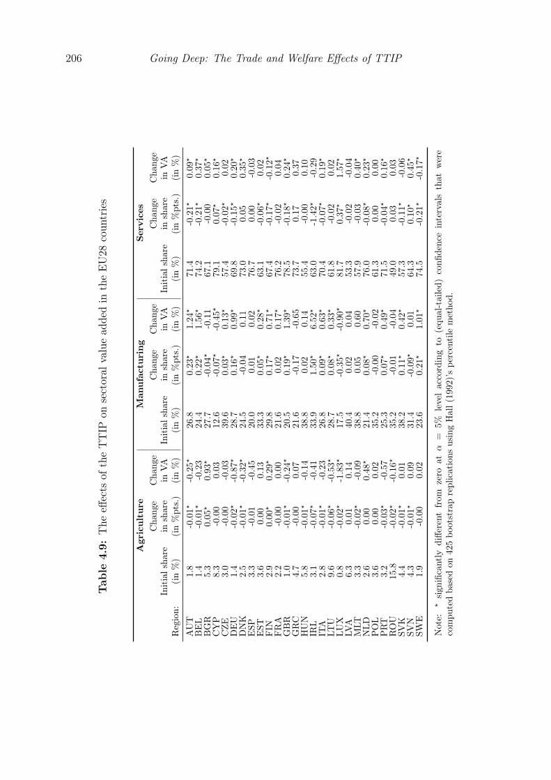
206 Going Deep: The Trade and Welfare Effects of TTIP
Tab
le4.9:
The
effects
oftheTTIP
onsectoral
valuead
dedin
theEU28
coun
tries
Agr
icult
ure
Man
ufa
cturi
ng
Ser
vice
sCha
nge
Cha
nge
Cha
nge
Cha
nge
Cha
nge
Cha
nge
Initials
hare
inshare
inVA
Initial s
hare
inshare
inVA
Initial s
hare
inshare
inVA
Region:
(in%)
(in%pts.)
(in%)
(in%)
(in%pts.)
(in%)
(in%)
(in%pts.)
(in%)
AUT
1.8
-0.01?
-0.25?
26.8
0.23?
1.24?
71.4
-0.21?
0.09?
BEL
1.4
-0.01?
-0.23
24.4
0.22?
1.56?
74.2
-0.21?
0.37?
BGR
5.3
0.05?
0.93?
27.7
-0.04?
-0.11
67.1
-0.00
0.05?
CYP
8.3
-0.00
0.03
12.6
-0.07?
-0.45?
79.1
0.07?
0.16?
CZE
3.0
-0.00
-0.03
39.6
0.03?
0.13?
57.4
-0.02?
0.02
DEU
1.4
-0.02?
-0.87?
28.7
0.16?
0.99?
69.8
-0.15?
0.20?
DNK
2.5
-0.01?
-0.32?
24.5
-0.04
0.11
73.0
0.05
0.35?
ESP
3.3
-0.01
-0.45
20.0
0.01
0.02
76.7
0.00
-0.03
EST
3.6
0.00
0.13
33.3
0.05?
0.28?
63.1
-0.06?
0.02
FIN
2.9
0.00?
0.29?
29.8
0.17?
0.71?
67.4
-0.17?
-0.12?
FRA
2.2
-0.00
0.00
21.6
0.02
0.17?
76.2
-0.02
0.04
GBR
1.0
-0.01?
-0.24?
20.5
0.19?
1.39?
78.5
-0.18?
0.24?
GRC
4.7
-0.00
0.07
21.6
-0.17
-0.65
73.7
0.17
0.37
HUN
5.8
-0.01?
-0.14
38.8
0.02
0.14
55.4
-0.00
0.10
IRL
3.1
-0.07?
-0.41
33.9
1.50?
6.52?
63.0
-1.42?
-0.29
ITA
2.8
-0.01?
-0.23
26.8
0.09?
0.63?
70.4
-0.07?
0.19?
LTU
9.6
-0.06?
-0.53?
28.7
0.08?
0.33?
61.8
-0.02
0.02
LUX
0.8
-0.02?
-1.83?
17.5
-0.35?
-0.90?
81.7
0.37?
1.57?
LVA
6.3
0.01
0.14
40.4
0.02
0.04
53.3
-0.02
-0.04
MLT
3.3
-0.02?
-0.09
38.8
0.05
0.60
57.9
-0.03
0.40?
NLD
2.6
0.00
0.48?
21.4
0.08?
0.70?
76.0
-0.08?
0.23?
POL
3.6
0.00
0.02
35.2
-0.00
-0.02
61.3
0.00
0.00
PRT
3.2
-0.03?
-0.57
25.3
0.07?
0.49?
71.5
-0.04?
0.16?
ROU
15.8
-0.02?
-0.16?
35.2
-0.01
-0.04
49.0
0.03
0.03
SVK
4.4
-0.01?
0.01
38.2
0.11?
0.42?
57.3
-0.11?
-0.06
SVN
4.3
-0.01?
0.09
31.4
-0.09?
0.01
64.3
0.10?
0.45?
SWE
1.9
-0.00
0.02
23.6
0.21?
1.01?
74.5
-0.21?
-0.17?
Note:
?sign
ificantly
diffe
rent
from
zero
atα
=5%
levelaccordingto
(equ
al-tailed)
confi
denceintervalsthat
were
compu
tedba
sedon
425bo
otstrapreplications
usingHall(1992)’spe
rcentile
metho
d.

Chapter 4 207
Figure 4.6: Sectoral value added: TTIP-induced changes-4
-20
24
68
in %
Publ
ic s
ervi
ces
Trad
e se
rvic
esBu
sine
ss s
ervi
ces
Dw
ellin
gsFi
nanc
ial s
ervi
ces
Con
stru
ctio
nM
achi
nery
nec
Rec
reat
ion
Che
mic
als
Com
mun
icat
ion
Insu
ranc
eTr
ansp
ort n
ecPa
per p
rodu
cts
Mea
t Pro
duct
sM
inin
gEl
ectri
city
Met
al p
rodu
cts
USA
-4-2
02
46
8in
%
Publ
ic s
ervi
ces
Busi
ness
ser
vice
sTr
ade
serv
ices
Dw
ellin
gsM
achi
nery
nec
Con
stru
ctio
nC
hem
ical
sR
ecre
atio
nFi
nanc
ial s
ervi
ces
Mot
or v
ehic
les
Tran
spor
t nec
Mea
t Pro
duct
sM
etal
pro
duct
sC
omm
unic
atio
nPe
trole
um, C
oal
Pape
r pro
duct
sEl
ectri
city
Elec
troni
cs
Germany
95% CI VA Growth
-8-6
-4-2
02
in %
Publ
ic s
ervi
ces
Trad
e se
rvic
esBu
sine
ss s
ervi
ces
Dw
ellin
gsC
onst
ruct
ion
Min
ing
Fina
ncia
l ser
vice
sC
omm
unic
atio
nC
hem
ical
sEl
ectri
city
Tran
spor
t nec
Mea
t Pro
duct
sR
ecre
atio
nPa
per p
rodu
cts
Mac
hine
ry n
ecM
otor
veh
icle
sIn
sura
nce
Met
al p
rodu
cts
Min
eral
s ne
c
Canada
-2.5
-2-1
.5-1
-.50
in %
Publ
ic s
ervi
ces
Trad
e se
rvic
esBu
sine
ss s
ervi
ces
Dw
ellin
gsC
onst
ruct
ion
Tran
spor
t nec
Fina
ncia
l ser
vice
sR
ecre
atio
nM
achi
nery
nec
Mea
t Pro
duct
sC
hem
ical
sC
omm
unic
atio
nEl
ectro
nics
Mot
or v
ehic
les
Insu
ranc
eEl
ectri
city
Petro
leum
, Coa
lFe
rrous
met
als
Pape
r pro
duct
s
Japan
95% CI VA Growth
Note: Equal-tailed confidence intervals based on 425 bootstrap samples and Hall (1992)’s percentilemethod. Sectors in every panel ordered along shares in total value added, in decreasing order fromleft to right. Sectors with initial shares in total value added < 1% not shown.

208 Going Deep: The Trade and Welfare Effects of TTIP
As exemplary TTIP outsiders we show sectoral value added changes for Canada andJapan. In Canada, most of the important sectors experience a decline in value added,most notably in “Motor Vehicles,” “Minerals nec,” “Machinery nec,” and “Metal products.”The sectors that gain, “Mining,” “Paper products,” and “Insurance,” tend to be locatedat early stages of the production chain. This is well in line with the argument laid outabove, that third countries gain from the increase in production in the TTIP countriesthrough an increase in the demand for intermediates. In Japan, which is not an importantsource country of intermediate inputs for the TTIP regions, value added declines in allimportant sectors.
4.4.6 Welfare Effects of the TTIP
Our simulation predicts that the TTIP will bring about significant real income gainsfor the EU countries and the United States, but also for many other countries. Figure4.7 presents welfare effects with confidence bands for all countries, Table 4.10 providesnumbers for selected individual countries and average effects for the world’s regions.17
In the EU, real income is predicted to go up by .43% on average, in the United Statesby .49%. Within the EU, Ireland stands out with a predicted real income increase by3.1%, followed by Luxembourg (1.1%). Moreover, welfare effects within the EU tend tobe larger for the Western and Northern European countries and smaller for the Centraland Southern European economies. With the exception of Greece, all TTIP countries’predicted gains are significantly different from zero at the 5% level.
Out of the 110 non-TTIP countries, 60 are predicted to gain, and for 50 of them thereal income effects are significant at the 5% level. For 33 non-TTIP countries, we findsignificantly negative predicted welfare effects. Among the non-TTIP winners are manydeveloping countries from Central America, Oceania, South Asia and Sub-Saharan Africaand the primarily developing countries grouped in the “Rest of World.” Also, countriesclose the EU, such as Turkey and the Balkans (collected in the “Rest of Europe”) gainfrom the TTIP. Arguably, the average gains for these regions are small (between .01 and.08), however, these make a strong case against the conjecture that the TTIP would beharmful to the developing world. Increased demand for final and intermediate goods in theTTIP countries counteracts negative trade diversion effects, benefitting countries that areintegrated into the TTIP partners production networks or which are important suppliersof raw materials. Trade diversion effects are less problematic for countries whose sectoral
17Regional effects are weighted averages using real GDP in 2011 as weights.

Chapter 4 209
Figure 4.7: Simulated changes on real income with the TTIP
LVA ROU POL BGR SVK CZE ESP PRT FIN FRA ITA CYP HUN EST SWE LTU AUT DNKGRC
NLDSVN USA DEU PRI GBR
BELMLT
HRV
LUX
IRL
0.5
11.
52
2.5
33.
5Pr
edic
ted
real
inco
me
chan
ge in
%
TTIP countries
NZLDOM
VEN
CMRISR
MDGRWA
MWI
URY
XEFIND
KHM
XSETURSLV
UGA
GTM
ARE
PHL
COLPRYTUNBGD
JAM
BLR
VNMLAOXCBPAKUKR
NGA
EGYLKAXER
MARETHALBGHA
ARMNPLTZAMUSHKG
XNASENXOC
JOR
BWA
PAN
ECU
KEN
GEO
GINXSA
MDA
ZWE
TGOXWF
KGZBEN
0.0
5.1
.15
.2Pr
edic
ted
real
inco
me
chan
ge in
%
Non-TTIP countries: Winners
TTO
QATKWT
AZE
KAZ
ZMB
OMNBRN
TWN
RUS
BFA
SAU
MEXCHLPERXSMIRN CIV
XSU
XACXNF
NOR
MNGBHR
MYSNICKORCHEXSC CRICHNHNDZAFNAMCANTHA IDN JPNSGPXTWBOLARGAUSMOZXEA
XCF
BRABLZ
XEC
XWS
-.6-.4
-.20
.2Pr
edic
ted
real
inco
me
chan
ge in
%
Non-TTIP countries: Losers
Real income change equal-tailed 95% CI
Note: The figure shows predicted real income changes (in %) for all 140 countries/regions included inour analysis. (Equal-tailed) confidence intervals are computed based on 425 bootstrap replicationsusing Hall (1992)’s percentile method.

210 Going Deep: The Trade and Welfare Effects of TTIP
Table 4.10: Welfare effects by regions
Real income change(in %) 95% CI
TTIP Countries 0.46 [0.354, 0.513]
EU28 0.43 [0.313, 0.478]USA 0.49 [0.396, 0.554]
Non-TTIP Regions -0.02 [-0.035, -0.004]
ASEAN -0.01 [-0.021, -0.007]AUS & NZL -0.01 [-0.014, 0.001]Alianza del Pacifico -0.06 [-0.081, -0.038]Canada -0.02 [-0.042, 0.002]Central America 0.01 [0.001, 0.022]Central Asia -0.03 [-0.058, 0.035]China -0.03 [-0.033, -0.020]EFTA -0.04 [-0.070, 0.018]East Asia -0.02 [-0.028, -0.015]Eurasian CU -0.11 [-0.195, 0.084]MERCOSUR -0.01 [-0.009, 0.002]Middle East & North Africa -0.02 [-0.034, 0.023]Oceania 0.08 [0.064, 0.094]Oil exporters -0.10 [-0.149, 0.011]Rest of Europe 0.06 [0.032, 0.074]Rest of World 0.05 [0.034, 0.059]SACU -0.02 [-0.029, -0.014]South Asia 0.02 [0.011, 0.031]Sub-Saharan Africa 0.02 [-0.008, 0.066]Turkey 0.02 [0.009, 0.033]
World 0.20 [0.155, 0.226]
Note: Regional changes are computed as real GDP-weighted averages of coun-try effects. (Equal-tailed) confidence intervals are computed based on 425 boot-strap replications using Hall (1992)’s percentile method.
production structure is complementary to those of TTIP regions, which tends to be truefor the less developed economies. This may also explain why welfare effects for Canadaare predicted to be negative even though Canada is closely integrated with the UnitedStates. The largest losses are expected to occur in the oil-producing countries in theMiddle East which compete directly with North American and Central Asian producersin supplying the TTIP regions. Moreover, countries far away from either of the two TTIPregions, such as the East and South East Asian economies including China, Korea, and

Chapter 4 211
Japan lose from the TTIP. The industrialized economies in the Far East are likely harmedbecause their production structure is relatively similar to the TTIP countries. Moreover,because of their remoteness, these countries are of less importance to the TTIP countriesas suppliers of intermediate and final goods and hence, benefit less from an increase indemand. Summing up all countries’ gains and losses, weighted by their shares in realworld GDP, we find that the world as whole gains from the TTIP in terms of an increasein real GDP by .2%.
4.5 Conclusion
A number of systemically relevant preferential trade agreements (PTAs) are under ne-gotiation. The largest of these mega-regionals is the proposed Transatlantic Trade andInvestment Partnership (TTIP). In this paper, we use the multi-country, multi-industryRicardian trade model of Caliendo and Parro (2015) extended to include non-tariff bar-riers to trade and trade in services to assess the potential effects of the TTIP on theglobal pattern of trade, production, and welfare. The framework features internationaland cross-sectoral production linkages and therefore allows taking into account globallyfragmented value chains and regional production networks. Hence, the model frameworkcombined with rich data on 38 sectors in 140 countries or regions from the GTAP databaseis well suited to analyze the effects of the TTIP, a deep trade agreement aimed at ad-dressing the important features of 21st century trade: fragmented value chains, trade inservices, and non-tariff barriers to trade.
The main assumption of our quantitative experiment is that, in addition to eliminatingall tariffs between the EU and the United States, the TTIP will lower the costs of non-tariffmeasures by the same amount as existing bilateral agreements have, on average, reducednon-tariff barriers. We use the gravity equation implied by the model to estimate the tradecost reductions achieved by existing shallow and deep PTAs, as well as the unobservedparameters of the model. We simulate the model to quantify the trade, production, andwelfare effects of the TTIP.
We find that the potential effects of the TTIP are quite substantial: real incomeis predicted to increase by .43% and .49% in the EU and United States, respectively.We find positive predicted effects for many other countries, including large parts of thedeveloping world, and for the world on average. Positive effects in third countries aredriven by the increase in income and demand in the TTIP regions, that benefits suppliersof consumption goods, intermediate goods, and raw materials. Some countries, including

212 Going Deep: The Trade and Welfare Effects of TTIP
the oil producers in the Middle East and the industrialized economies in East Asia, areexpected to lose from the TTIP.
Our framework is closely related to the “New Quantitative Trade Theory” literature.This literature (surveyed by Costinot and Rodriguez-Clare, 2014) uses parsimonious trademodels combined with structural estimation to conduct counterfactual analyses. For thetime being, the methodology has barely been used for the analysis of real trade policyinitiatives; most existing work still uses more traditional large-scale computable generalequilibrium (CGE) models. While the availability of industry-level trade and outputdata, the information on existing PTAs, and state-of-the-art of econometric tools hasmuch improved over the last years, there is particular need for further work in at leastfour areas: First, the unbiased econometric estimation of structural parameters requiresquasi-experimental variation and appropriate methods. This remains an important areafor future work. Second, top-down approaches to non-tariff trade barriers, as used in thispaper, differ from bottom-up assessments based on Francois et al. (2009). Understandingthis discrepancy is key if one wants to narrow the interval of welfare predictions found instudies with different approaches to non-tariff barriers to trade. Third, both traditionalCGE models as well as the frameworks surveyed by Costinot and Rodriguez-Clare (2014)neglect foreign direct investment. This is particularly important in the transatlanticcontext. Fourth, estimates presented in this paper may underestimate the true effects asthey do not account for effects of trade liberalization on the incentives to develop newproducts or engineer new processes. A tractable dynamic framework would thus be highlywelcome.

Appendix A.4
Table A4.11: Overview of sectors and aggregation levels
GTAP sectors Sector aggregates used in the analysis Broad classification1 Paddy rice 1 Grains & Crops Agriculture2 Wheat 1 Grains & Crops Agriculture3 Cereal grains nec 1 Grains & Crops Agriculture4 Vegetables, fruit, nuts 1 Grains & Crops Agriculture5 Oil seeds 1 Grains & Crops Agriculture6 Sugar cane, sugar beet 1 Grains & Crops Agriculture7 Plant-based fibers 1 Grains & Crops Agriculture8 Crops nec 1 Grains & Crops Agriculture9 Cattle, sheep, goats, horses 2 Cattle, sheep, goats, horses Agriculture10 Animal products nec 2 Livestock & Meat Products Agriculture11 Raw milk 2 Livestock & Meat Products Agriculture12 Wool, silk-worm cocoons 2 Livestock & Meat Products Agriculture13 Forestry 3 Forestry Agriculture14 Fishing 4 Fishing Agriculture15 Coal 5 Mining (coal, oil, gas) Manufacturing16 Oil 5 Mining (coal, oil, gas) Manufacturing17 Gas 5 Mining (coal, oil, gas) Manufacturing18 Minerals nec 6 Minerals nec Manufacturing19 Meat: cattle, sheep, goats, horses 2 Livestock & Meat Products Manufacturing20 Meat products nec 2 Livestock & Meat Products Manufacturing21 Vegetable oils and fats 7 Livestock & Meat Products Manufacturing22 Dairy products 7 Livestock & Meat Products Manufacturing23 Processed rice 1 Grains & Crops Manufacturing24 Sugar 7 Livestock & Meat Products Manufacturing25 Food products nec 7 Livestock & Meat Products Manufacturing26 Beverages and tobacco products 7 Livestock & Meat Products Manufacturing27 Textiles 8 Textiles Manufacturing28 Wearing apparel 9 Wearing apparel Manufacturing29 Leather products 10 Leather products Manufacturing30 Wood products 11 Wood products Manufacturing31 Paper products, publishing 12 Paper products, publishing Manufacturing32 Petroleum, coal products 13 Petroleum, coal products Manufacturing33 Chemical, rubber, plastic prods 14 Chemical, rubber, plastic prods Manufacturing34 Mineral products nec 15 Mineral products nec Manufacturing35 Ferrous metals 16 Ferrous metals Manufacturing36 Metals nec 17 Metals nec Manufacturing37 Metal products 18 Metal products Manufacturing38 Motor vehicles and parts 19 Motor vehicles and parts Manufacturing39 Transport equipment nec 20 Transport equipment nec Manufacturing40 Electronic equipment 21 Electronic equipment Manufacturing41 Machinery and equipment nec 22 Machinery and equipment nec Manufacturing42 Manufactures nec 23 Manufactures nec Manufacturing43 Electricity 24 Electricity Services44 Gas manufacture, distribution 25 Gas manufacture, distribution Services45 Water 26 Water Services46 Construction 27 Construction Services47 Trade 28 Trade Services48 Transport nec 29 Transport nec Services49 Sea transport 30 Sea transport Services50 Air transport 31 Air transport Services51 Communication 32 Communication Services52 Financial services nec 33 Financial services nec Services53 Insurance 34 Insurance Services54 Business services nec 35 Business services nec Services55 Recreation and other services 36 Recreation and other services Services56 PubAdmin/Defence/Health/Education 37 PubAdmin/Defence/Health/Education Services57 Dwellings 38 Dwellings Services

214 Going Deep: The Trade and Welfare Effects of TTIPTab
leA4.12:IV
Results
forAgriculterala
ndMan
ufacturing
Sectors
Sector:
(1)
(2)
(3)
(4)
(5)
(6)
(7)
(8)
(9)
(10)
(11)
(12)
lnτ
-2.310∗∗∗
-2.441∗∗∗
-3.385∗∗∗
-3.156∗∗∗
-6.021
-3.695∗∗∗
-2.498∗∗∗
-4.913∗∗∗
-1.613∗∗∗
-2.939∗∗∗
-2.774∗∗∗
-4.697∗∗∗
(0.148)
(0.163)
(0.553)
(0.657)
(4.199)
(0.690)
(0.093)
(0.285)
(0.398)
(0.299)
(0.263)
(0.241)
Shallow
0.249∗∗
-0.261∗∗
-0.024
-0.182
1.269∗∗
0.357∗∗
0.188∗∗
0.079
-0.023
0.208∗∗
0.073
0.146∗
(0.106)
(0.116)
(0.156)
(0.210)
(0.591)
(0.144)
(0.082)
(0.092)
(0.113)
(0.095)
(0.075)
(0.079)
Deep
0.401∗∗∗
-0.204
0.086
0.076
0.830
0.364∗∗∗
0.289∗∗∗
0.294∗∗∗
0.502∗∗∗
0.637∗∗∗
0.476∗∗∗
0.526∗∗∗
(0.118)
(0.125)
(0.150)
(0.209)
(0.542)
(0.129)
(0.091)
(0.082)
(0.106)
(0.093)
(0.077)
(0.078)
lnDist
-0.537∗∗∗
-0.561∗∗∗
-0.415∗∗∗
-0.670∗∗∗
-0.592∗∗∗
-0.439∗∗∗
-0.632∗∗∗
-0.562∗∗∗
-0.682∗∗∗
-0.648∗∗∗
-0.719∗∗∗
-0.928∗∗∗
(0.040)
(0.042)
(0.053)
(0.072)
(0.155)
(0.049)
(0.034)
(0.031)
(0.035)
(0.034)
(0.029)
(0.030)
Con
tiguity
0.831∗∗∗
0.695∗∗∗
0.942∗∗∗
0.725∗∗∗
0.457∗∗
0.607∗∗∗
0.762∗∗∗
0.451∗∗∗
0.638∗∗∗
0.786∗∗∗
0.775∗∗∗
0.675∗∗∗
(0.089)
(0.080)
(0.101)
(0.124)
(0.211)
(0.087)
(0.080)
(0.064)
(0.089)
(0.086)
(0.076)
(0.077)
Com
Lang
0.015
0.109∗
-0.086
-0.051
-0.552∗∗∗
0.025
0.206∗∗∗
0.201∗∗∗
0.375∗∗∗
0.294∗∗∗
0.280∗∗∗
0.422∗∗∗
(0.058)
(0.062)
(0.074)
(0.084)
(0.195)
(0.058)
(0.047)
(0.044)
(0.051)
(0.048)
(0.044)
(0.045)
Colon
y0.127
0.070
0.343∗∗∗
0.046
0.347
0.070
0.296∗∗∗
0.267∗∗∗
0.403∗∗∗
0.467∗∗∗
0.470∗∗∗
0.414∗∗∗
(0.086)
(0.088)
(0.097)
(0.109)
(0.242)
(0.078)
(0.074)
(0.065)
(0.092)
(0.084)
(0.070)
(0.073)
CurColon
y1.093∗∗
0.718
1.373∗∗∗
-0.115
-2.453∗
-0.140
0.666
0.808
0.698
0.806
0.803
0.639
(0.506)
(0.495)
(0.390)
(0.363)
(1.296)
(0.275)
(0.583)
(0.503)
(1.255)
(1.083)
(0.906)
(0.564)
Com
Col
0.302∗∗∗
0.435∗∗∗
0.138
0.339∗∗∗
0.221
0.323∗∗∗
0.604∗∗∗
0.162∗∗
0.102
0.335∗∗∗
0.364∗∗∗
0.630∗∗∗
(0.081)
(0.100)
(0.116)
(0.125)
(0.283)
(0.086)
(0.070)
(0.063)
(0.080)
(0.084)
(0.067)
(0.074)
Observation
s243624
90274
22304
28274
6669
85350
531429
801095
699145
175800
223734
317824
AdjustedR
20.292
0.337
0.318
0.302
0.413
0.251
0.300
0.325
0.464
0.445
0.450
0.417
Sector:
(13)
(14)
(15)
(16)
(17)
(18)
(19)
(20)
(21)
(22)
(23)
lnτ
-5.463∗∗∗
-4.743∗∗∗
-2.804∗∗∗
-1.187∗∗∗
-3.691∗∗∗
-2.167∗∗∗
-3.670∗∗∗
-2.315∗∗∗
-2.184∗∗∗
-3.181∗∗∗
-2.275∗∗∗
(1.220)
(0.218)
(0.225)
(0.368)
(0.452)
(0.226)
(0.239)
(0.287)
(0.231)
(0.166)
(0.204)
Shallow
0.807∗∗∗
0.201∗∗∗
0.081
0.188∗
0.611∗∗∗
0.247∗∗∗
0.296∗∗∗
0.136
0.467∗∗∗
0.196∗∗∗
0.169∗∗
(0.186)
(0.071)
(0.078)
(0.102)
(0.121)
(0.080)
(0.091)
(0.089)
(0.078)
(0.066)
(0.077)
Deep
0.672∗∗∗
0.317∗∗∗
0.157∗∗
0.665∗∗∗
0.752∗∗∗
0.307∗∗∗
0.896∗∗∗
0.409∗∗∗
0.242∗∗∗
0.175∗∗∗
0.251∗∗∗
(0.205)
(0.072)
(0.073)
(0.093)
(0.102)
(0.078)
(0.101)
(0.086)
(0.081)
(0.062)
(0.076)
lnDist
-1.120∗∗∗
-0.765∗∗∗
-0.730∗∗∗
-0.708∗∗∗
-0.529∗∗∗
-0.851∗∗∗
-0.802∗∗∗
-0.358∗∗∗
-0.748∗∗∗
-0.696∗∗∗
-0.581∗∗∗
(0.066)
(0.030)
(0.030)
(0.037)
(0.038)
(0.029)
(0.033)
(0.030)
(0.029)
(0.024)
(0.030)
Con
tiguity
0.717∗∗∗
0.551∗∗∗
0.790∗∗∗
0.648∗∗∗
0.422∗∗∗
0.654∗∗∗
0.581∗∗∗
0.531∗∗∗
0.431∗∗∗
0.470∗∗∗
0.662∗∗∗
(0.124)
(0.068)
(0.073)
(0.079)
(0.076)
(0.080)
(0.078)
(0.066)
(0.082)
(0.064)
(0.076)
Com
Lang
-0.248∗∗
0.173∗∗∗
0.231∗∗∗
0.121∗∗
0.134∗∗
0.383∗∗∗
0.224∗∗∗
0.155∗∗∗
0.299∗∗∗
0.241∗∗∗
0.302∗∗∗
(0.098)
(0.044)
(0.045)
(0.055)
(0.055)
(0.046)
(0.051)
(0.045)
(0.044)
(0.038)
(0.043)
Colon
y0.135
0.280∗∗∗
0.342∗∗∗
0.241∗∗∗
0.274∗∗∗
0.612∗∗∗
0.335∗∗∗
0.305∗∗∗
0.472∗∗∗
0.466∗∗∗
0.383∗∗∗
(0.139)
(0.065)
(0.071)
(0.073)
(0.079)
(0.080)
(0.088)
(0.066)
(0.077)
(0.064)
(0.074)
CurColon
y-1.053
1.252∗∗∗
0.921∗
1.006∗∗
0.344
0.731
0.453
0.381
2.041∗
1.366∗
1.247∗
(1.579)
(0.385)
(0.475)
(0.464)
(0.420)
(0.860)
(1.014)
(0.742)
(1.103)
(0.735)
(0.720)
Com
Col
0.140
0.505∗∗∗
0.514∗∗∗
0.264∗∗∗
0.430∗∗∗
0.560∗∗∗
0.974∗∗∗
0.512∗∗∗
0.555∗∗∗
0.633∗∗∗
0.436∗∗∗
(0.146)
(0.069)
(0.071)
(0.087)
(0.081)
(0.078)
(0.090)
(0.080)
(0.082)
(0.069)
(0.068)
Observ ation
s22745
1544089
337582
302429
182487
628789
157463
112560
320393
2212282
371077
AdjustedR
20.385
0.344
0.372
0.318
0.338
0.468
0.536
0.384
0.526
0.458
0.409
Note:
Estim
ates
ofim
porter,e
xporter,an
dHS6-digitprod
uctfix
edeff
ects
notshow
n.Stan
dard
errors
(inpa
renthe
ses)
areclusteredat
thecoun
try-pa
irlevel.Sh
ea’sPartial
R2is0.19
forshallow
and0.23
fordeep
PTAs.
*,**
and***indicate
statisticalsign
ificanceat
the10,5an
d1%
level,respectively.
PTA
dummiesinstrumentedwithcontagionindicesala
Martinet
al.(2012)
orBaldw
inan
dJa
imovich(2012).

Chapter 4 215
Tab
leA4.13:IV
Results
forServiceSectors
Sector:
(24)
(25)
(26)
(27)
(28)
(29)
(30)
(31)
(32)
(33)
(34)
(35)
(36)
(37)
Shallow
0.298∗∗∗
0.141∗∗
0.229∗∗∗
0.169∗∗∗
0.129∗∗∗
0.182∗∗∗
0.024
0.175∗∗∗
0.221∗∗∗
0.160∗∗∗
0.152∗∗∗
0.267∗∗∗
0.142∗∗∗
0.178∗∗∗
(0.051)
(0.062
)(0.031)
(0.064
)(0.037)
(0.032)
(0.055)
(0.040)
(0.031)
(0.040)
(0.033)
(0.035)
(0.037)
(0.036)
Deep
0.438∗∗∗
0.389∗∗∗
0.377∗∗∗
0.302∗∗∗
0.580∗∗∗
0.399∗∗∗
0.413∗∗∗
0.123∗∗
0.294∗∗∗
0.490∗∗∗
0.338∗∗∗
0.559∗∗∗
0.238∗∗∗
0.367∗∗∗
(0.076)
(0.089
)(0.053)
(0.081
)(0.056)
(0.050)
(0.075)
(0.055)
(0.051)
(0.060)
(0.054)
(0.054)
(0.052)
(0.057)
lnDist
-0.053∗∗
0.032
0.006
-0.036
-0.019
-0.007
0.012
0.004
-0.002
-0.036∗∗
-0.009
-0.017
-0.016
-0.044∗∗∗
(0.024)
(0.026
)(0.014)
(0.022
)(0.015)
(0.014)
(0.020)
(0.015)
(0.014)
(0.016)
(0.014)
(0.014)
(0.015)
(0.015)
Con
tiguity
2.104∗∗∗
0.573∗∗∗
0.492∗∗∗
0.347∗∗∗
0.414∗∗∗
0.432∗∗∗
0.491∗∗∗
0.319∗∗∗
0.359∗∗∗
0.317∗∗∗
0.418∗∗∗
0.250∗∗∗
0.424∗∗∗
0.407∗∗∗
(0.158)
(0.095
)(0.067)
(0.078
)(0.063)
(0.061)
(0.071)
(0.055)
(0.058)
(0.065)
(0.063)
(0.059)
(0.062)
(0.066)
Com
Lang
0.029
0.065∗
0.023
0.058∗
0.004
-0.022
0.018
-0.033
0.00
4-0.014
-0.013
-0.013
0.020
-0.016
(0.032)
(0.038
)(0.019)
(0.032
)(0.022)
(0.019)
(0.030)
(0.021)
(0.019)
(0.023)
(0.020)
(0.021)
(0.020)
(0.021)
Colon
y0.345∗∗∗
0.328∗∗∗
0.378∗∗∗
0.235∗∗∗
0.390∗∗∗
0.404∗∗∗
0.334∗∗∗
0.347∗∗∗
0.312∗∗∗
0.255∗∗∗
0.246∗∗∗
0.205∗∗∗
0.307∗∗∗
0.321∗∗∗
(0.088)
(0.079
)(0.064)
(0.073
)(0.058)
(0.060)
(0.069)
(0.055)
(0.057)
(0.072)
(0.062)
(0.051)
(0.058)
(0.066)
CurColon
y-0.258
0.106
-0.059
0.091
0.23
8-0.051
-0.289
0.777
0.427
0.943
0.689
0.383
0.443
0.258
(0.957)
(1.024
)(0.964)
(1.245
)(1.100)
(0.891)
(1.043)
(0.755)
(1.193)
(1.292)
(1.087)
(1.234)
(0.814)
(1.051)
Com
Col
-0.007
-0.107∗∗
-0.068∗∗∗
0.024
-0.023
-0.024
-0.102∗∗∗
-0.016
-0.053∗∗
-0.058∗
-0.037
-0.078∗∗∗
-0.093∗∗∗
0.012
(0.045)
(0.053
)(0.024)
(0.039
)(0.027)
(0.024)
(0.036)
(0.027)
(0.025)
(0.030)
(0.024)
(0.027)
(0.028)
(0.026)
Observation
s13546
11368
14434
14518
14518
14518
14518
14518
14518
14518
14518
14518
14518
1451
8AdjustedR
20.968
0.952
0.959
0.901
0.956
0.955
0.918
0.948
0.952
0.950
0.956
0.963
0.955
0.939
Note:
Estim
ates
ofim
porter
andexpo
rter
fixed
effects
notshow
n.Stan
dard
errors
(inpa
renthe
ses)
areclusteredat
thecoun
try-pa
irlevel.
Shea’s
Partial
R2is
0.19
forshallow
and0.23
fordeep
PTAs.
*,**
and***indicate
statisticalsign
ificanceat
the10,5an
d1%
level,respectively.PTA
dummiesinstrumentedwithcontagionindicesala
Martinet
al.(2012)
orBaldw
inan
dJa
imov
ich(2012).

216 Going Deep: The Trade and Welfare Effects of TTIP
Tab
leA4.14:OLS
Results
forAgriculterala
ndMan
ufacturing
Sectors
Sector:
(1)
(2)
(3)
(4)
(5)
(6)
(7)
(8)
(9)
(10)
(11)
(12)
lnτ
-2.329∗∗∗
-2.203∗∗∗
-3.452∗∗∗
-2.907∗∗∗
-11.126∗∗∗
-4.254∗∗∗
-2.439∗∗∗
-5.000∗∗∗
-1.727∗∗∗
-3.316∗∗∗
-2.899∗∗∗
-4.783∗∗∗
(0.143)
(0.154)
(0.540)
(0.586)
(3.834)
(0.643)
(0.085)
(0.234)
(0.312)
(0.280)
(0.254)
(0.235)
Shallow
0.093∗∗
-0.019
-0.085
-0.033
-0.344∗
0.034
0.113∗∗∗
0.073∗∗
0.067
-0.012
0.019
0.068∗
(0.042)
(0.054)
(0.067)
(0.072)
(0.184)
(0.052)
(0.039)
(0.037)
(0.042)
(0.042)
(0.036)
(0.039)
Deep
0.384∗∗∗
0.277∗∗∗
0.073
0.213∗∗∗
-0.025
0.422∗∗∗
0.429∗∗∗
0.234∗∗∗
0.372∗∗∗
0.389∗∗∗
0.349∗∗∗
0.450∗∗∗
(0.053)
(0.063)
(0.074)
(0.080)
(0.191)
(0.060)
(0.050)
(0.044)
(0.054)
(0.050)
(0.045
)(0.047)
lnDist
-0.555∗∗∗
-0.456∗∗∗
-0.425∗∗∗
-0.633∗∗∗
-0.900∗∗∗
-0.461∗∗∗
-0.613∗∗∗
-0.570∗∗∗
-0.689∗∗∗
-0.706∗∗∗
-0.747∗∗∗
-0.950∗∗∗
(0.027)
(0.030)
(0.037)
(0.043)
(0.093)
(0.030)
(0.026)
(0.025)
(0.026)
(0.026)
(0.023
)(0.024)
Con
tiguity
0.827∗∗∗
0.754∗∗∗
0.929∗∗∗
0.749∗∗∗
0.413∗∗
0.610∗∗∗
0.780∗∗∗
0.446∗∗∗
0.610∗∗∗
0.754∗∗∗
0.748∗∗∗
0.658∗∗∗
(0.087)
(0.078)
(0.100)
(0.119)
(0.204)
(0.086)
(0.078)
(0.064)
(0.088)
(0.084)
(0.075
)(0.076)
Com
Lang
0.028
0.100∗
-0.089
-0.059
-0.493∗∗∗
0.042
0.218∗∗∗
0.204∗∗∗
0.378∗∗∗
0.295∗∗∗
0.278∗∗∗
0.423∗∗∗
(0.057)
(0.061)
(0.074)
(0.083)
(0.186)
(0.057)
(0.046)
(0.043)
(0.051)
(0.048)
(0.044
)(0.045)
Colon
y0.141∗
0.095
0.344∗∗∗
0.049
0.444∗
0.106
0.306∗∗∗
0.246∗∗∗
0.349∗∗∗
0.436∗∗∗
0.448∗∗∗
0.403∗∗∗
(0.084)
(0.084)
(0.096)
(0.108)
(0.228)
(0.076)
(0.074)
(0.065)
(0.095)
(0.087)
(0.072
)(0.073)
CurColon
y1.057∗∗
0.810
1.366∗∗∗
-0.072
-2.657∗∗
-0.198
0.647
0.820
0.732
0.808
0.814
0.632
(0.505)
(0.498)
(0.388)
(0.360)
(1.275)
(0.261)
(0.584)
(0.506)
(1.273)
(1.089)
(0.913
)(0.564)
Com
Col
0.291∗∗∗
0.439∗∗∗
0.144
0.351∗∗∗
0.214
0.314∗∗∗
0.592∗∗∗
0.163∗∗∗
0.106
0.335∗∗∗
0.368∗∗∗
0.625∗∗∗
(0.080)
(0.099)
(0.116)
(0.121)
(0.281)
(0.085)
(0.070)
(0.063)
(0.080)
(0.083)
(0.067
)(0.073)
Observ ation
s244386
90501
22337
28326
6684
8551
0533495
802975
701957
176517
224570
318983
AdjustedR
20.292
0.339
0.318
0.304
0.421
0.252
0.30
00.326
0.465
0.446
0.450
0.417
Sector:
(13)
(14)
(15)
(16)
(17)
(18)
(19)
(20)
(21)
(22)
(23)
lnτ
-7.003∗∗∗
-4.815∗∗∗
-2.760∗∗∗
-1.527∗∗∗
-4.742∗∗∗
-2.266∗∗∗
-3.796∗∗∗
-2.352∗∗∗
-2.180∗∗∗
-3.142∗∗∗
-2.317∗∗∗
(1.156)
(0.205)
(0.205)
(0.356)
(0.415)
(0.207)
(0.225)
(0.283)
(0.227)
(0.157)
(0.191)
Shallow
-0.018
0.064∗
0.058
-0.056
0.084∗
0.119∗∗∗
0.253∗∗∗
0.123∗∗∗
0.249∗∗∗
0.169∗∗∗
0.087∗∗
(0.084)
(0.036)
(0.039)
(0.048)
(0.045)
(0.039)
(0.047)
(0.043)
(0.039)
(0.033)
(0.035)
Deep
0.250∗∗∗
0.354∗∗∗
0.278∗∗∗
0.504∗∗∗
0.371∗∗∗
0.333∗∗∗
0.708∗∗∗
0.297∗∗∗
0.397∗∗∗
0.302∗∗∗
0.278∗∗∗
(0.095)
(0.046)
(0.045)
(0.056)
(0.054)
(0.046)
(0.053)
(0.047)
(0.043)
(0.037)
(0.044)
lnDist
-1.265∗∗∗
-0.769∗∗∗
-0.709∗∗∗
-0.759∗∗∗
-0.644∗∗∗
-0.854∗∗∗
-0.838∗∗∗
-0.379∗∗∗
-0.735∗∗∗
-0.671∗∗∗
-0.581∗∗∗
(0.051)
(0.024)
(0.024)
(0.029)
(0.028)
(0.024)
(0.027)
(0.023)
(0.023)
(0.019)
(0.023)
Con
tiguity
0.707∗∗∗
0.556∗∗∗
0.799∗∗∗
0.632∗∗∗
0.397∗∗∗
0.656∗∗∗
0.550∗∗∗
0.517∗∗∗
0.462∗∗∗
0.486∗∗∗
0.662∗∗∗
(0.121)
(0.067)
(0.073)
(0.078)
(0.073)
(0.079)
(0.079)
(0.065)
(0.080)
(0.064)
(0.075)
Com
Lang
-0.207∗∗
0.181∗∗∗
0.236∗∗∗
0.129∗∗
0.154∗∗∗
0.391∗∗∗
0.214∗∗∗
0.155∗∗∗
0.311∗∗∗
0.247∗∗∗
0.311∗∗∗
(0.096)
(0.044)
(0.045)
(0.054)
(0.053)
(0.046)
(0.051)
(0.045)
(0.044)
(0.038)
(0.043)
Colon
y0.180
0.279∗∗∗
0.343∗∗∗
0.241∗∗∗
0.265∗∗∗
0.598∗∗∗
0.313∗∗∗
0.282∗∗∗
0.485∗∗∗
0.463∗∗∗
0.370∗∗∗
(0.133)
(0.067)
(0.072)
(0.072)
(0.074)
(0.083)
(0.089)
(0.065)
(0.079)
(0.065)
(0.076)
CurColon
y-1.198
1.235∗∗∗
0.921∗∗
0.975∗∗
0.248
0.730
0.460
0.401
2.006∗
1.369∗
1.246∗
(1.571)
(0.380)
(0.467)
(0.461)
(0.422)
(0.853)
(1.028)
(0.744)
(1.082)
(0.725)
(0.717)
Com
Col
0.109
0.498∗∗∗
0.513∗∗∗
0.272∗∗∗
0.408∗∗∗
0.557∗∗∗
0.980∗∗∗
0.515∗∗∗
0.530∗∗∗
0.629∗∗∗
0.430∗∗∗
(0.146)
(0.069)
(0.070)
(0.087)
(0.078)
(0.077)
(0.090)
(0.080)
(0.081)
(0.068)
(0.067)
Observ ation
s22815
1548959
338654
303154
182827
631455
158267
112875
321309
2221122
372259
AdjustedR
20.389
0.344
0.373
0.319
0.341
0.468
0.536
0.384
0.527
0.458
0.411
Note:
Estim
ates
ofim
porter,expo
rter,an
dHS
6-digitprod
uctfix
edeff
ects
notshow
n.Stan
dard
errors
(in
parentheses)
areclustered
atthe
coun
try-pa
irlevel.*,
**an
d**
*indicate
statisticalsign
ificanceat
the10,5an
d1%
level,respectively.

Chapter 4 217
Tab
leA4.15:OLS
Results
forServiceSectors
Sector:
(24)
(25)
(26)
(27)
(28)
(29)
(30)
(31)
(32)
(33)
(34)
(35)
(36)
(37)
Shallow
-0.022
-0.040
-0.032∗∗
-0.034
-0.003
-0.018
-0.010
-0.008
-0.016
-0.027
-0.032∗∗
0.007
-0.028∗
-0.069∗∗∗
(0.020)
(0.029
)(0.013)
(0.026)
(0.016)
(0.014)
(0.022)
(0.016)
(0.013)
(0.016)
(0.014)
(0.014)
(0.014)
(0.015)
Deep
0.017
0.055
0.029
0.003
0.222∗∗∗
0.060∗∗
0.208∗∗∗
-0.013
0.015
0.127∗∗∗
0.122∗∗∗
0.188∗∗∗
0.026
0.085∗∗∗
(0.035)
(0.043
)(0.026)
(0.037)
(0.026)
(0.024)
(0.036)
(0.026)
(0.025)
(0.029)
(0.026)
(0.024)
(0.026)
(0.026)
lnDist
-0.148∗∗∗
-0.033
-0.071∗∗∗
-0.101∗∗∗
-0.086∗∗∗
-0.075∗∗∗
-0.021
-0.034∗∗∗
-0.065∗∗∗
-0.104∗∗∗
-0.059∗∗∗
-0.097∗∗∗
-0.064∗∗∗
-0.109∗∗∗
(0.019)
(0.020
)(0.011)
(0.017)
(0.012)
(0.011)
(0.015)
(0.011)
(0.011)
(0.013)
(0.011)
(0.011)
(0.012)
(0.012)
Con
tiguity
2.110∗∗∗
0.573∗∗∗
0.489∗∗∗
0.342∗∗∗
0.391∗∗∗
0.425∗∗∗
0.476∗∗∗
0.327∗∗∗
0.362∗∗∗
0.312∗∗∗
0.420∗∗∗
0.242∗∗∗
0.423∗∗∗
0.412∗∗∗
(0.156)
(0.094
)(0.065)
(0.076)
(0.062)
(0.059)
(0.070)
(0.054)
(0.056)
(0.063)
(0.062)
(0.057)
(0.060)
(0.064)
Com
Lang
0.040
0.060
0.035∗
0.069∗∗
0.009
-0.016
0.016
-0.023
0.016
-0.013
-0.005
-0.005
0.031
-0.005
(0.031)
(0.038
)(0.018)
(0.032)
(0.021)
(0.019)
(0.029)
(0.020)
(0.018)
(0.023)
(0.020)
(0.020)
(0.020)
(0.021)
Colon
y0.327∗∗∗
0.312∗∗∗
0.362∗∗∗
0.224∗∗∗
0.359∗∗∗
0.386∗∗∗
0.322∗∗∗
0.345∗∗∗
0.302∗∗∗
0.240∗∗∗
0.239∗∗∗
0.196∗∗∗
0.295∗∗∗
0.306∗∗∗
(0.085)
(0.076
)(0.060)
(0.071)
(0.056)
(0.057)
(0.067)
(0.052)
(0.054)
(0.070)
(0.060)
(0.047)
(0.056)
(0.063)
CurColon
y-0.244
0.128
-0.050
0.091
0.258
-0.032
-0.274
0.783
0.434
0.958
0.690
0.393
0.448
0.271
(0.968)
(1.046
)(0.975)
(1.260)
(1.138)
(0.910)
(1.076)
(0.748)
(1.197)
(1.321)
(1.089)
(1.251)
(0.817)
(1.055)
Com
Col
-0.016
-0.109∗∗
-0.074∗∗∗
0.015
-0.028
-0.028
-0.101∗∗∗
-0.021
-0.060∗∗
-0.061∗∗
-0.043∗
-0.083∗∗∗
-0.097∗∗∗
0.003
(0.045)
(0.053
)(0.023)
(0.038)
(0.027)
(0.024)
(0.036)
(0.027)
(0.024)
(0.030)
(0.024)
(0.026)
(0.028)
(0.025)
Observation
s13780
11523
14674
14760
1476
014760
14760
14760
14760
14760
14760
14760
14760
14760
AdjustedR
20.969
0.952
0.960
0.902
0.956
0.956
0.918
0.949
0.953
0.951
0.956
0.964
0.955
0.94
0
Note:
Estim
ates
ofim
porter
andexpo
rter
fixed
effects
notshow
n.Stan
dard
errors
(inpa
rentheses)
areclusteredat
thecoun
try-pa
irlevel.*,
**an
d***indicate
statisticalsign
ificance
atthe10,5an
d1%
level,respectively.


Chapter 5
Parameter Uncertainty in NQTTModels∗
5.1 Introduction
One defining feature of the New Quantitative Trade Theory (NQTT) is the tight linkbetween theory and empirics. This link is created by structural estimation of unobservedmodel parameters based on the same model that is used for the counterfactual analysisand based on the same data that is used for calibration of the model’s observable moments.Hence, unobserved structural parameters are chosen in a way that is consistent with boththe model and the observable moments used in the subsequent analysis. However, theestimated parameters depend on the particular dataset we have at hand and, dependingon the precision of the estimation, provide only a more or less noisy measure of the trueparameters guiding the structural model. The estimates are random variables and so arethe model predictions based on these estimates. Moreover, expected values of non-linearfunctions of random variables, such as trade and welfare effects in NQTT models, divergefrom values at estimated means of parameters. Ignoring the random nature of estimatedparameters leads to biased predictions of model outcomes, with the bias depending onthe degree of non-linearity of the model and the degree of uncertainty surrounding theestimates.
The aim of this chapter is to draw attention to the issues of uncertainty and bias insimulation outcomes of models calibrated with estimated parameters. We propose that
∗This chapter is based on joint work with Rahel Aichele and Gabriel Felbermayr.

220 Parameter Uncertainty in NQTT Models
acknowledging uncertainty of model predictions caused by uncertainty about the model’sparameters is a natural step forward for counterfactual analyses based on NQTT models.
With few exceptions, the issue of parameter uncertainty has been overseen by thisliterature. Lai and Trefler (2002), Anderson and Yotov (2016), and Shapiro (2015) arenoteworthy exceptions. Lai and Trefler (2002) compute analytical standard errors forgains from trade estimates based on a structural gravity model, which is feasible onlyfor very parsimonious model structures. Anderson and Yotov (2016) bootstrap regressioncoefficients from a structural gravity equation to obtain standard errors for inference onthe general equilibrium effects of a gravity model. Shapiro (2015) conducts a bootstrapto obtain confidence intervals for model predictions based on the structural parameterestimates’ asymptotic normal distribution. We aim to contribute to this recent literatureby showing how the bootstrap can be used to estimate the bias caused by the non-linearity of the model. Moreover, we discuss different concepts of confidence intervals formodel outcomes that can be obtained from the bootstrap exercise. We also take a firststep towards understanding the relationship between the degree of parameter uncertaintyand the quantitative importance of the bias and the uncertainty surrounding the modelpredictions.
To that end, we conduct a bootstrap to quantify the bias and the extent of uncertaintyof the simulated effects of the policy scenario analyzed in the previous chapter, that is, theimplementation of the Transatlantic Trade and Investment Partnership (TTIP). Based on425 bootstrap samples drawn from our original dataset underlying the estimation of thestructural parameters, we find an average bias of 7% for the welfare effects predicted by themodel. The bias tends to be positive for positive welfare changes and negative otherwise,implying that the simulation results overestimate the true effects in absolute terms. Sinceour simulation outcomes were small to begin with, the estimated bias in absolute terms(for example, .013 percentage points for the EU, .017 percentage points for the US) israther small. In accordance with the theory, we find that the bias increases in the degreeof uncertainty surrounding the parameter estimates. We repeat the bootstrap and thesimulation exercise based on only 50% of the observations from the original sample, andfind that the average bias increases to 11%.
Our results show that even in an application characterized by very precisely estimatedparameters, accounting for uncertainty is important to tell apart model outcomes that arenot statistically significant from those that are. Our counterfactual analysis of the TTIPpredicts negative welfare effects for 50 out of 140 countries or regions, however, only in twothirds of these cases are the effects significantly different from zero at the 95% level. Someof the largest losses, predicted for the oil exporting countries from the Middle East and

Chapter 5 221
the countries forming the Eurasian Customs Union, turn out to be insignificant. On thewinning side, we find that 12% of the predicted positive effects fall victim to accountingfor uncertainty. The predicted positive effect for the TTIP countries, except for Greece,and for the world average are strongly significant. Hence, in the case of our application,accounting for parameter uncertainty does not impair the validity of the main results ofthe counterfactual analysis.
5.2 A Bootstrap of the Standard Error, ConfidenceInterval, and Bias of Model Predictions
In the previous chapter, we conducted a counterfactual experiment based on a generalequilibrium trade model to analyze the effects of the introduction of the TTIP. We usedobservable and estimated unobservable parameters to calibrate the model and then solvedthe model for the changes in endogenous outcomes, such as prices, wages, trade patterns,and welfare. From a more general point of view we may characterize the outcomes ofsuch a counterfactual analysis by a structural relationship W := W (X t,O, κ), relatingthe change in some endogeneous variable of interestW to the change in a policy variable κfor a given set of observable moments X t describing the current state of the economy. Thefunctional relationshipW (·) depends on the particular model structure chosen to describeproduction and consumption relationships in the economy, characterized by structuralparameters O.
In the TTIP scenario discussed in the previous chapter, Wi may denote, for example,the real income change of country i following the reduction of trade costs between theUnited States and the EU28 countries, captured by changes in the respective elementsof the bilateral trade cost matrix κ.1 The functional relationship W (·) is determined bythe set of equilibrium conditions and the functional form assumptions governing demandand supply. The set of observable moments X t is given by the matrix of trade shares πt,expenditure levels X t, and value added wLt. The structural parameters comprise theelasticities of the utility and production functions, α,β, and γ, the dispersion parametersof the sectoral productivity distributions θ, and the sectoral elasticities of the trade cost
1Note that for simplicitiy’s sake, we do not use the hat notation here to differentiate changes in variablesfrom their levels as we did in the previous chapter, but rather define symbols as levels or changes in thetext.

222 Parameter Uncertainty in NQTT Models
function ρdeep with respect to deep trade agreements.2 In this particular setup, someof the elements of O, namely, α,β, and γ, are observable. More precisely, they maybe replaced by observable moments, since according to the model’s agents’ first orderconditions, in equlibrium the elasticities of the utility and production functions are equalto expenditure shares for final goods and cost shares of inputs, respectively.
The remaining elements of O, which we collect in the vector Θ := [θ,ρdeep] need tobe estimated. We use ΘN to denote a consistent estimate of Θ obtained from one par-ticular sample of size N . Since the dataset is only one draw of the underlying datagenerating process characterized by the population moments Θ, ΘN is a random variable.Abstracting from other sources of uncertainty, for example uncertainty about the func-tional relationships summarized inW (·) or measurement error in the observable momentsX t, our outcome variable of interest from the simulation, W (ΘN) (as well as all otherendogenous variables of the model) can be viewed as a measurable function of the randomvariables ΘN . Therefore, our model-based predictions of the effects of the TTIP inheritthe uncertainty present in the data used to estimate the model’s parameters.
For many problems of this type, in particular for cases where the derivative of W (Θ)
with respect to Θ is simple to obtain, the Delta method can be used to approximate thevariance of a function of random variables. In our case, however, W (Θ) is the solutionto a complicated system of equations rendering analytical derivation of its derivativesinfeasible. For problems of this type, the bootstrap theory provides us with a computa-tionally burdensome but feasible alternative to estimate the standard error of a functionof random variables. In the following subsections we briefly discuss some results fromeconometrics theory on the estimation of standard errors, confidence intervals, and thebias of non-linear estimators by means of a bootstrap. This discussion follows Cameronand Trivedi (2005) and Horowitz (2001) to whom we refer the reader for details.
5.2.1 Some Results from the Bootstrapping Literature
The theory of the bootstrap builds on the fact that every independently drawn samplefrom the dataset used to estimate ΘN inherits some of the properties of the underlyingdata generating process and that we can draw any desired number B of such samples. Forevery sample b = 1, ..., B (of size N), we can calculate parameter estimates Θb
N to obtainan empirical distribution of Θb
Ns that approximates the distribution of ΘN . Moreover, for
2Note that X t and O are only subsets of the complete sets of observable moments and structural param-eters of the model. Which subsets are needed depends on the variable of interest W and the structureof the model.

Chapter 5 223
each of the B ΘbNs, we can compute the corresponding value ofW (Θb
N) and thereby obtainan empirical distribution ofW (Θb
N), which approximates the distribution ofW (ΘN). Thebootstrap works under mild conditions regarding the underlying data generating process,which we assume to be fulfilled.
5.2.1.1 Bootstrapping Standard Error
Based on B bootstrap samples (of size N) and the corresponding values of our modeloutcomes
{W (Θ1
N), ...,W (ΘbN), ...,W (ΘB
N)}, it is straightforward to compute an estimate
of the sampling variance as
s2W =
1
B − 1
B∑b=1
(W (Θb
N)−W (ΘbN))2 with W (Θb
N) =1
B
B∑b=1
W (ΘbN), (5.1)
which consistently estimates σ2W , the variance of W (ΘN).
5.2.1.2 Confidence Intervals
A confidence interval (CI) [Wlow,Whigh] of significance level α for W := W (Θ) is definedby
Prob [Wlow < W < Whigh] = 1− α. (5.2)
Let WN := W (ΘN) and let GN(·) denote the distribution of the sampling error WN −Wconditional on N , the size of the original sample. Then, for any α1, α2 satisfying α1, α2 > 0
and α1 + α2 = α, the confidence bounds [Wlow,Whigh] are given by
CI : [WN − w1−α2 ,WN − wα1 ], (5.3)
where wx denotes the xth percentile of GN(·), that is, GN(wα1) = α1 and GN(w1−α2) =
1−α2. The interpretation of the CI is as follows. Suppose a large number of samples of sizeN could be drawn from the true data generating process characterized by E[W (ΘN)] = W .Then, in (1− α)× 100 percent of all cases, confidence intervals computed in accordancewith Equation (5.3) above would contain the true value. In other words, the chance thata so-defined confidence interval includes the true parameter is (1− α)× 100 percent.
To compute the confidence bounds, one needs to know the sampling distribution GN(·)and choose α1, α2 subject to α1 + α2 = α. Typically, α1, α2 are chosen such as to obtaineither equal-tailed CIs by setting α1 = α2 = α/2 or symmetric CIs for which α1, α2 are

224 Parameter Uncertainty in NQTT Models
chosen to yield bounds which are centered around the estimate WN , so that | −w1−α2| =|−wα2|. If the sampling distribution is symmetric, equal-tailed and symmetric confidenceintervals for a given significance level are identical.
In general, the sampling distribution GN is neither symmetric nor known. Standardasymptotic theory, however, implies that GN converges to a normal distribution withmean zero and variance σ2
W as N goes to infinity.3 σ2W may be replaced by a consistent
estimator such as s2W (cp. Equation 5.1). Hence, for large enough values of N , the
standard CI
CIS : [WN − σW z1−α2 ,WN − σW zα1 ], (5.4)
where zx denotes the xth percentile of the standard normal distribution, well approximatesthe CI as defined in Equation (5.3).
An alternative estimate of the confidence bounds proposed by Efron (1981) can beobtained from the bootstrapping exercise. It uses the fact that the sampling distributionof the bootstrap estimates, W b
N −WN , converges to the distribution of WN −W , the sam-pling distribution of our original estimate, and hence, the percentiles of the distributionof the bootstrapped W b
N ’s are consistent estimates of the percentiles of the (unobserved)distribution of WN . This so-called bootstrap percentile method yields the confidence inter-val
CIBP1 : [W bα1, W b
1−α2] ⇔ [WN + wbα1
, WN + wb1−α2], (5.5)
where wbx is the xth percentile of the bootstrap distribution of W bN −WN . As discussed
by Hall (1992), CIBP1 is problematic if the distribution WN − W is asymmetric sincethe implied coverage probability as defined in Equation (5.2) generally does not equalα = α1 + α2, unless GN(·) is symmetric.4 To address this concern, Hall (1992) proposesanother bootstrap percentile method based CI
CIBP2 : [WN − wb1−α2, WN − wbα1
], (5.6)
3To be precise, we are considering the normal asymptotic distribution of√N(WN −W ) with mean 0 and
asymptotic variance Nσ2W , since the distribution of WN −W degenerates in the limit of N .
4CIBPI approximates W + wα1 , W + w1−α2 . Hence, the coverage probability implied by CIBP1 isProb[W + wα1
< W < W + w1−α2] = GN (−wα1
) − GN (−w1−α2) Q (1 − α1 − α2). GN (−wα1
) −GN (−w1−α2
) = (1−α) holds for symmetric distributions GN (·), but generally not in asymmetric cases.

Chapter 5 225
which is not quite as intuitive as CIBP1, but more appealing from a theoretical perspectiveand equally simple to obtain from the bootstrap replications ofW . The reason is that theconfidence bounds given in Equation (5.3) depend on the distribution of −(WN −W ) =
(W −WN) which has the opposite skewness of the distribution of (WN −W ). Therefore,being based on the quantiles of the distribution of W b
N − WN which converges to thedistribution of WN − W , CIBP1 gets the skewness wrong. CIBP2, instead, is based onthe quantiles of the distribution of −(W b
N −WN) which converges to the distribution ofW −WN and, therefore, gets the skewness right.
Neither of the percentile method based CIs, however, achieves asymptotic refinement.The validity of CIBP1 and CIBP2, alike the validity of CIS, relies on a sufficiently largesample size N (in addition to a sufficiently large number of bootstrap replications) sinceonly then do the bootstrapped percentiles wbx provide a good approximation to wx, the per-centiles of GN(·). CIs offering asymptotic refinement can be obtained with the percentile-tmethod or with adjustments for bias and acceleration as proposed by Efron (1987). Inour framework, however, both approaches are technically feasible but computationallyburdensome due to the fact that every bootstrap of W b
N requires numerically solving acomplex system of non-linear equations. To apply the percentile-t method, we would needa bootstrap within each bootstrap to obtain a standard error estimate for every replica-tion b, since an analytical solution even with the help of the delta method is not withinreach. In fact, we mainly resorted to bootstrapping in the first place exactly becauseof the difficulty to obtain a standard error for WN by conventional methods. Likewise,for the bias-corrected and accelerated CIs, a non-parametric estimate of the accelerationconstant would be equally burdensome to obtain.
5.2.1.3 The Bias
The non-linearity of W (·) implies that the expected value of W differs from the functionevaluated at the expected value of ΘN . The bias, E [W (ΘN)−W (Θ)], can be approxi-mated by a second-order Taylor expansion of W around the true value Θ. To convey theintuition, we consider first the case where W (·) is a scalar-valued function. The bias isthen approximated by
BN =∂W
∂θE [θN − θ] +
1
2
∂2W
∂θ2E [θN − θ]2 =
1
2
∂2W
∂θ2σ2θ , (5.7)
where we have used the fact that E [θN − θ] = 0 if θN is a consistent estimator of θ.The bias is larger the stronger the curvature of W and, in accordance with Jensen’sinequality, positive if W is convex and negative otherwise. Moreover, the bias increases

226 Parameter Uncertainty in NQTT Models
in the variance of the estimate, σ2θ . It vanishes as σ2
θ goes to zero; hence, W (θN) is aconsistent estimator for W (θ).
Naturally, these results carry over to the case of our vector-valued function W (Θ), forwhich we obtain
BN =1
2E[(ΘN −Θ)′
∂2W
∂ΘΘ′(ΘN −Θ)
](5.8)
as a second-order approximation to the bias E [W (ΘN)] −W (Θ). In practice, the mag-nitude of BN is unknown since it depends on the matrix of second derivatives of W (·)evaluated at the unknown population moments Θ. However, it can be estimated by meansof a bootstrap that makes use of the fact that the average of the bootstrapped quanti-ties W (Θb
N), b = 1, ..., B provides an estimator for W (ΘN) whose behaviour mimicks thebehaviour of W (ΘN) as an estimator for W (Θ). In other words, the bootstrap uses thedeviation of the E
[W (Θb
N)]fromW (ΘN) to approximate the deviation of E[W (ΘN)] from
W (Θ). A second-order approximation of E[W (Θb
N)]−W (ΘN), the bias of the bootstrap
estimate of W (ΘN), yields
BBN =
1
2E[(Θb
N −ΘN)′∂2W
∂ΘNΘ′N(Θb
N −ΘN)
]. (5.9)
Importantly, E[W (Θb
N)]−W (ΘN) can be approximated by 1
B
∑Bb=1 W (Θb
N) −W (ΘN)
with arbitrary precision by increasing the number of bootstrapped samples. Hence, thebootstrap provides us with a feasible estimate of BN , the bias caused by the non-linearityof W (·) Moreover, as detailed in Horowitz (2001), Bb
N converges to BN faster than BN
approaches zero; hence, we can use BbN to obtain a bias-corrected estimate of our quantity
of interest as
WBbc (ΘN) = W (ΘN)−BB
N . (5.10)
5.3 Application: Predicted Welfare Effects of the TTIP
We now apply the insights from the bootstrapping literature summarized in the previoussection to a simulation study of the welfare effects of the TTIP. The application is basedon the same model and the same dataset as the analysis in Chapter 4. Our model outcomeof interest is the welfare effect (change in real income, by country) as defined in Equation(4.8) in Chapter 4. We bootstrap 425 replications of the country-specific welfare effects

Chapter 5 227
to calculate confidence intervals and assess the magnitude of the bias for this particularapplication.
The dataset used to estimate the structural parameters consists of bilateral trade flowsfor 140 countries and 38 sectors in the year 2011 and proxies for bilateral trade costs typi-cally used in the gravity literature. In the agricultural and manufacturing sectors (sectors1-23) trade flows are disaggregated at the product level. The coefficients of interest arethe sectoral productivity dispersions θ, which equals the inverse of the elasticity of tradewith respect to trade costs and can be obtained as the coefficient on tariffs, and the elas-ticity of trade costs with respect to the incidence of a deep or shallow preferential tradeagreement (PTA), ρdeep, ρshallow.5 Since the latter are likely endogeneous to the level oftrade cost or other unobserved determinants of bilateral trade, we instrument the deepand shallow PTA dummies with a contagion index. Country-fixed effects control for thecountry-level determinants implied by the theory and potentially unobserved confound-ing factors. We run separate regressions for 37 sectors to obtain sector-specific estimatesof θj, ρjdeep, ρ
jshallow which we collect in the vectors θ, ρdeep, and ρshallow.6 By running
regressions sector by sector, we implicitly assume independence of errors across sectors.However, standard errors are expected to be correlated within country pairs. To accountfor clustering within country pairs in the bootstrap-based inference, we sample countrypairs rather that country-pair (-product) observations. That is, the bootstrap samplingrandomly chooses country pairs from the original dataset using all available product-levelobservations within the pair. The sampling is done with replacement to ensure inde-pendence of individual draws. Throughout this chapter we present results based on 425bootstrap replications of parameter estimates θb, ρbdeep and the corresponding simulationoutcomes W b.
To shed some light on the relationship between the degree of parameter uncertainty andthe degree of uncertainty surrounding the model outcomes, we repeat the whole exercisestarting out with a smaller sample, where we randomly dropped 50% of all observationsin the estimation stage. Moreover, we consider the case where in the simulation stageonly uncertainty of the estimates of θ is taken into account, holding fixed the values ofρdeep at the level of the original estimates.
5Note that our particular definition of the TTIP scenario does not need the estimates of ρshallow, however,they are clearly important as control variables in the estimation and would be needed in the simulationif alternative scenarios were considered.
6As detailed in Chapter 4, we set the PTA effect to zero in sector 38 (“Dwellings”), where we do notobserve positive trade flows, and we use θ = 5.9 for the services sector, where θ cannot be estimatedsince we do not observe tariffs.

228 Parameter Uncertainty in NQTT Models
Table 5.1: Parameter estimates: Sectoral productivity dispersion θ
(1) (2) (3) (4) (5) (6)
Full sample 50% sampleSector name Sector 1/θ t-stat N 1/θ t-stat N
Grains & Crops 1 -2.310∗∗∗ -15.85 243,624 -2.232∗∗∗ -12.99 122,027Livestock farming 2 -2.441∗∗∗ -13.99 90,274 -2.434∗∗∗ -13.25 45,114Forestry 3 -3.385∗∗∗ -6.42 22,304 -2.889∗∗∗ -3.79 11,140Fishing 4 -3.156∗∗∗ -4.70 28,274 -3.369∗∗∗ -3.99 14,218Mining 5 -6.021∗ -1.72 6,669 -10.275∗ -1.94 3,292Minerals nec 6 -3.695∗∗∗ -5.26 85,350 -4.082∗∗∗ -4.86 42,669Meat products 7 -2.498∗∗∗ -29.48 531,429 -2.542∗∗∗ -24.09 265,841Textiles 8 -4.913∗∗∗ -16.89 801,095 -4.826∗∗∗ -15.83 400,672Wearing apparel 9 -1.613∗∗∗ -4.95 699,145 -1.514∗∗∗ -4.77 349,963Leather products 10 -2.939∗∗∗ -9.80 175,800 -2.635∗∗∗ -8.03 87,824Wood products 11 -2.774∗∗∗ -10.35 175,800 -2.784∗∗∗ -9.29 87,824Paper products 12 -4.697∗∗∗ -20.50 223,734 -4.633∗∗∗ -17.29 111,859Petroleum, Coal 13 -5.463∗∗∗ -4.65 317,824 -5.163∗∗∗ -3.24 158,986Chemicals 14 -4.743∗∗∗ -22.18 22,745 -4.753∗∗∗ -21.22 11,281Minerals 15 -2.804∗∗∗ -12.81 1,544,089 -2.875∗∗∗ -11.35 772,538Ferrous metals 16 -1.187∗∗∗ -4.40 337,582 -1.000∗∗∗ -4.35 168,691Metals nec 17 -3.691∗∗∗ -8.30 302,429 -3.787∗∗∗ -7.24 151,291Metal products 18 -2.167∗∗∗ -9.59 182,487 -2.309∗∗∗ -9.53 91,364Motor vehicles 19 -3.670∗∗∗ -15.97 628,789 -3.892∗∗∗ -13.87 314,373Transport eqpm. nec 20 -2.315∗∗∗ -7.76 157,463 -2.434∗∗∗ -6.95 78,827Electronics 21 -2.184∗∗∗ -9.74 112,560 -2.235∗∗∗ -8.62 56,295Machinery nec 22 -3.181∗∗∗ -19.90 320,393 -3.176∗∗∗ -19.25 160,523Manufactures nec 23 -2.275∗∗∗ -11.03 2,212,282 -2.197∗∗∗ -9.78 1,106,528
Note: Estimates of ρdeep (ρshallow) are reported in Table 5.2 (A5.6). Estimates of importer, exporter, and HS 6-digit prod-uct fixed effects and the standard gravity controls (lnDist, Contiguity, Common Language, Former Colony, Current Colony,Common Colonizer) not shown. Standard errors obtained from 425 bootstrap replication accounting for clustering at country-pair level. *, ** and *** indicate statistical significance at the 10, 5 and 1% level, respectively. PTA dummies instrumentedwith contagion indices a la Martin et al. (2012) or Baldwin and Jaimovich (2012).
5.3.1 Data and Estimation Results
Tables 5.1 and 5.2 show the estimated parameters of interest obtained from the gravityspecification with instrumental variables as described in the previous chapter.7 Columns(1)-(3) display the result from the full sample (equaling the estimates used for the simula-tions in the previous chapter), Columns (4)-(6) show the results for the same specificationbased on a dataset where we have randomly dropped 50% of observations in every sec-tor.8 With few exceptions, the loss of information leads to less precise estimates (smallert-values). Generally, however, ρdeep and θ are very precisely estimated also with only halfof the data and their magnitudes are remarkably stable.
7For the sake of completeness, Table A5.6 reports the estimates for the shallow PTA effects, which donot feature in our simulations.
8The number of observations in Column (6) is some times more or less than half the number of observationsin Column (3) because a few observations are not used in the regressions because of missing data orcollinearity with fixed effects.
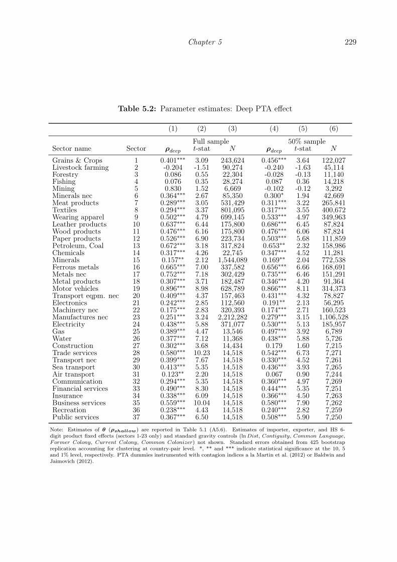
Chapter 5 229
Table 5.2: Parameter estimates: Deep PTA effect
(1) (2) (3) (4) (5) (6)
Full sample 50% sampleSector name Sector ρdeep t-stat N ρdeep t-stat N
Grains & Crops 1 0.401∗∗∗ 3.09 243,624 0.456∗∗∗ 3.64 122,027Livestock farming 2 -0.204 -1.51 90,274 -0.240 -1.63 45,114Forestry 3 0.086 0.55 22,304 -0.028 -0.13 11,140Fishing 4 0.076 0.35 28,274 0.087 0.36 14,218Mining 5 0.830 1.52 6,669 -0.102 -0.12 3,292Minerals nec 6 0.364∗∗∗ 2.67 85,350 0.300∗ 1.94 42,669Meat products 7 0.289∗∗∗ 3.05 531,429 0.311∗∗∗ 3.22 265,841Textiles 8 0.294∗∗∗ 3.37 801,095 0.317∗∗∗ 3.55 400,672Wearing apparel 9 0.502∗∗∗ 4.79 699,145 0.533∗∗∗ 4.97 349,963Leather products 10 0.637∗∗∗ 6.44 175,800 0.686∗∗∗ 6.45 87,824Wood products 11 0.476∗∗∗ 6.16 175,800 0.476∗∗∗ 6.06 87,824Paper products 12 0.526∗∗∗ 6.90 223,734 0.503∗∗∗ 5.68 111,859Petroleum, Coal 13 0.672∗∗∗ 3.18 317,824 0.653∗∗ 2.32 158,986Chemicals 14 0.317∗∗∗ 4.26 22,745 0.347∗∗∗ 4.52 11,281Minerals 15 0.157∗∗ 2.12 1,544,089 0.169∗∗ 2.04 772,538Ferrous metals 16 0.665∗∗∗ 7.00 337,582 0.656∗∗∗ 6.66 168,691Metals nec 17 0.752∗∗∗ 7.18 302,429 0.735∗∗∗ 6.46 151,291Metal products 18 0.307∗∗∗ 3.71 182,487 0.346∗∗∗ 4.20 91,364Motor vehicles 19 0.896∗∗∗ 8.98 628,789 0.866∗∗∗ 8.11 314,373Transport eqpm. nec 20 0.409∗∗∗ 4.37 157,463 0.431∗∗∗ 4.32 78,827Electronics 21 0.242∗∗∗ 2.85 112,560 0.191∗∗ 2.13 56,295Machinery nec 22 0.175∗∗∗ 2.83 320,393 0.174∗∗∗ 2.71 160,523Manufactures nec 23 0.251∗∗∗ 3.24 2,212,282 0.279∗∗∗ 3.15 1,106,528Electricity 24 0.438∗∗∗ 5.88 371,077 0.530∗∗∗ 5.13 185,957Gas 25 0.389∗∗∗ 4.47 13,546 0.497∗∗∗ 3.92 6,789Water 26 0.377∗∗∗ 7.12 11,368 0.438∗∗∗ 5.88 5,726Construction 27 0.302∗∗∗ 3.68 14,434 0.179 1.60 7,215Trade services 28 0.580∗∗∗ 10.23 14,518 0.542∗∗∗ 6.73 7,271Transport nec 29 0.399∗∗∗ 7.67 14,518 0.330∗∗∗ 4.52 7,261Sea transport 30 0.413∗∗∗ 5.35 14,518 0.436∗∗∗ 3.93 7,265Air transport 31 0.123∗∗ 2.20 14,518 0.067 0.90 7,244Communication 32 0.294∗∗∗ 5.35 14,518 0.360∗∗∗ 4.97 7,269Financial services 33 0.490∗∗∗ 8.30 14,518 0.444∗∗∗ 5.35 7,251Insurance 34 0.338∗∗∗ 6.09 14,518 0.366∗∗∗ 4.50 7,263Business services 35 0.559∗∗∗ 10.04 14,518 0.580∗∗∗ 7.90 7,262Recreation 36 0.238∗∗∗ 4.43 14,518 0.240∗∗∗ 2.82 7,259Public services 37 0.367∗∗∗ 6.50 14,518 0.508∗∗∗ 5.90 7,250
Note: Estimates of θ (ρshallow) are reported in Table 5.1 (A5.6). Estimates of importer, exporter, and HS 6-digit product fixed effects (sectors 1-23 only) and standard gravity controls (lnDist, Contiguity, Common Language,Former Colony, Current Colony, Common Colonizer) not shown. Standard errors obtained from 425 bootstrapreplication accounting for clustering at country-pair level. *, ** and *** indicate statistical significance at the 10, 5and 1% level, respectively. PTA dummies instrumented with contagion indices a la Martin et al. (2012) or Baldwin andJaimovich (2012).

230 Parameter Uncertainty in NQTT Models
5.3.2 Confidence Bounds for Welfare Effects
The main results from our bootstrapping exercise are summarized in Table 5.3 for 22countries or regions and the world. Table 5.4 presents disaggregated results for the 28EU countries, Table A5.7 has detailed results for the non-TTIP countries. Column (1) ofTables 5.3 and 5.4 shows the welfare effects obtained from solving the model for the originalparameter estimates ΘN .9 Columns (2)-(5) present the four different confidence intervalsdescribed in Section 5.2.1.2. The first result we want to highlight is that irrespectiveof the confidence interval we are looking, at most of the predicted welfare effects aresignificantly different from zero at the level of α = .05.10 With the exception of Greece,the predicted gains for all individual TTIP countries are strongly significant, and so is thepredicted gain for the world as a whole. Hence, in this particular application, accountingfor parameter uncertainty does not bring into question the qualitative results obtainedfrom the simulation study.
However, accounting for uncertainty allows to single out quantitative predictions,which, from a statistical point of view, cannot be differentiated from zero. Consider,for example, the welfare effect predicted for the Eurasian Customs Union (CU) in Table5.3, which is the largest negative effect among the 22 regions. According to three of thefour estimated confidence intervals, the effect is not statistically different from zero forα = .05. Similarly, the negative welfare effects for Central Asia and the EFTA are sur-rounded by a large degree of uncertainty, rendering the predictions insignificant. On thewinning side, we find that welfare gains predicted for Sub-Saharan Africa and CentralAmerica are not significant. In total, we find that the welfare effects for 17 out of 50countries who are predicted to lose from TTIP, and for 11 out of 90 countries who arepredicted to win, can, statistically, not be differentiated from zero.
Table 5.3 also shows that different concepts of confidence intervals may lead to differentconclusions regarding significance. Only in three cases do the four concepts consideredunanimously agree on insignificance for a given level of α (Sub-Saharan Africa, CentralAmerica, and Middle East & North Africa). The two symmetric confidence intervals,(CIS in Column (2), which relies on the normal approximation, and CIBP1 in Column(4), which uses the quantiles of the bootstrapped distribution of the welfare effects) arevery similar.
9The estimated welfare effects in Column (1) are equal to the results presented in Chapter 4.10Note that due to the fact that the choice of α = α1 + α2 does not always reflect a coverage probabilityof (1− α) ∗ 100, as discussed in Section 5.2.1.2, we do not generally refer to α as the significance level.

Chapter 5 231
Tab
le5.3:
Welfare
chan
ge,c
onfid
ence
intervals(α
=.0
5),a
ndbias:by
region
s
(1)
(2)
(3)
(4)
(5)
(6)
(7)
(8)
WN
CI S
CI BP
1CI BP
1CI BP
2B
ias
pwd
symm.(eq.-t.)
equa
l-tailed
symm.
equa
l-tailed
absolute
relative
(425,.0
5)Region/
Cou
ntry
(in%)
(in%)
(in%)
(in%)
(in%)
(in%pts.)
(in%)
(in%)
USA
0.49
3[0.416,0
.571]
[0.433,0
.592]
[0.408,0
.579]
[0.395,0
.553]
0.01
30.02
60.042
EU28
0.42
6[0.344,0
.508]
[0.372,0
.537]
[0.333,0
.519]
[0.314,0
.479]
0.01
70.04
00.075
Ocean
ia0.08
0[0.064,0
.096]
[0.068,0
.098]
[0.063,0
.097]
[0.062,0
.092]
0.00
20.02
00.010
Restof
Europ
e0.05
6[0.035,0
.077]
[0.044,0
.086]
[0.033,0
.080]
[0.026,0
.069]
0.00
30.05
00.064
Restof
World
0.04
4[0.031,0
.056]
[0.031,0
.056]
[0.031,0
.056]
[0.031,0
.057]
-0.001
0.01
60.013
SouthAsia
0.02
3[0.013,0
.034]
[0.015,0
.035]
[0.014,0
.033]
[0.012,0
.032]
0.00
00.02
00.022
Sub-Sa
haranAfrica
0.02
3[-0
.011,0
.057]
[-0.019,0
.054]
[-0.011,0
.057]
[-0.008,0
.065]
-0.001
0.06
30.371
Turkey
0.02
3[0.010,0
.035]
[0.014,0
.038]
[0.010,0
.035]
[0.007,0
.032]
0.00
10.04
70.051
Central
America
0.00
9[-0
.002,0
.020]
[-0.003,0
.019]
[-0.002,0
.019]
[-0.001,0
.020]
0.00
00.00
20.047
MERCOSU
R-0.005
[-0.011,-0.000]
[-0.012,-0.002]
[-0.011,-0.000]
[-0.009,0
.002]
-0.000
0.05
20.043
AUS&
NZL
-0.010
[-0.018,-0.003]
[-0.019,-0.004]
[-0.018,-0.003]
[-0.017,-0.001]
-0.000
0.00
20.023
ASE
AN
-0.014
[-0.021,-0.006]
[-0.021,-0.006]
[-0.021,-0.006]
[-0.021,-0.007]
-0.000
0.00
80.013
Mid.East&
N.A
frica
-0.016
[-0.045,0
.012]
[-0.056,0
.001]
[-0.043,0
.010]
[-0.034,0
.023]
-0.002
0.10
10.380
EastAsia
-0.019
[-0.026,-0.012]
[-0.025,-0.012]
[-0.026,-0.012]
[-0.026,-0.013]
0.00
00.00
30.010
SACU
-0.021
[-0.029,-0.014]
[-0.028,-0.013]
[-0.029,-0.013]
[-0.029,-0.014]
0.00
10.03
40.009
Can
ada
-0.024
[-0.046,-0.002]
[-0.044,-0.000]
[-0.046,-0.002]
[-0.048,-0.004]
0.00
10.05
80.069
China
-0.027
[-0.034,-0.021]
[-0.034,-0.022]
[-0.034,-0.021]
[-0.033,-0.021]
-0.000
0.00
90.006
Central
Asia
-0.030
[-0.078,0
.017]
[-0.095,-0.001]
[-0.078,0
.017]
[-0.060,0
.034]
-0.003
0.10
60.534
EFTA
-0.040
[-0.086,0
.006]
[-0.097,-0.010]
[-0.083,0
.004]
[-0.070,0
.018]
-0.002
0.05
20.354
Al.
delP
acifico
-0.064
[-0.086,-0.042]
[-0.084,-0.042]
[-0.086,-0.042]
[-0.086,-0.044]
0.00
10.01
60.025
Oilexpo
rters
-0.102
[-0.186,-0.018]
[-0.216,-0.056]
[-0.195,-0.008]
[-0.148,0
.013]
-0.007
0.06
50.626
EurasianCU
-0.104
[-0.245,0
.038]
[-0.297,-0.018]
[-0.237,0
.030]
[-0.189,0
.090]
-0.008
0.07
71.484
World
0.20
2[0.168,0
.236]
[0.178,0
.249]
[0.164,0
.240]
[0.156,0
.226]
0.00
70.03
30.022
Note:pwd(B,t
)deno
tesim
pliedpe
rcentage
deviationof
bias
estimateno
texceed
withprob
ability
(1−t)∗
100
=95%
givenB
=425bo
otstrapsamples.pwdis
calculated
usingtheap
prox
imatemetho
dprop
osed
byCam
eron
andTrivedi
(2005),Ch.
11.Con
fidence
intervalsin
Colum
ns(2)-(5)an
dbias
estimateas
defin
edin
thetext.Relative
bias
inpe
rcentofWN.

232 Parameter Uncertainty in NQTT ModelsTab
le5.4:
Welfare
chan
ge,c
onfid
ence
intervals(α
=.0
5),a
ndbias:EU28
coun
tries
(1)
(2)
(3)
(4)
(5)
(6)
(7)
(8)
WN
CI S
CI BP
1CI BP
1CI BP
2B
ias
pwd(4
25,.
05)
symm.(eq.-tailed)
equa
l-tailed
symm.
equa
l-tailed
absolute
relative
(in%)
(in%)
(in%)
(in%)
(in%)
(in%pts.)
(in%)
(in%)
IRL
3.11
5[2.502, 3
.727]
[2.593,3
.785]
[2.515,3
.715]
[2.445,3
.637]
0.06
82.18
20.405
LUX
1.08
7[0.857,1
.318]
[0.890,1
.356]
[0.857,1
.317]
[0.819,1
.284]
0.02
52.32
80.177
HRV
0.76
5[0.699,0
.832]
[0.711,0
.846]
[0.697,0
.834]
[0.685,0
.820]
0.00
30.43
30.026
MLT
0.75
7[0.551,0
.962]
[0.613,1
.014]
[0.543,0
.970]
[0.499,0
.900]
0.03
44.55
70.203
BEL
0.66
2[0.527,0
.798]
[0.570,0
.845]
[0.511,0
.813]
[0.480,0
.755]
0.02
53.71
90.101
GBR
0.54
9[0.456,0
.643]
[0.482,0
.667]
[0.440,0
.658]
[0.432,0
.617]
0.01
83.22
70.057
DEU
0.51
1[0.391,0
.630]
[0.445,0
.672]
[0.382,0
.639]
[0.349,0
.576]
0.02
44.69
20.207
SVN
0.44
2[0.188,0
.696]
[0.289,0
.791]
[0.200,0
.685]
[0.094,0
.595]
0.03
06.69
10.985
NLD
0.44
1[0.363,0
.520]
[0.385,0
.543]
[0.359,0
.524]
[0.340,0
.498]
0.01
32.88
20.051
GRC
0.40
7[0.114,0
.700]
[0.237,0
.821]
[0.123,0
.692]
[-0.006,0
.578]
0.03
48.26
11.567
DNK
0.37
0[0.303,0
.436]
[0.315,0
.449]
[0.301,0
.438]
[0.291,0
.425]
0.00
82.21
80.043
AUT
0.35
5[0.267,0
.444]
[0.308,0
.478]
[0.264,0
.447]
[0.233,0
.403]
0.01
64.63
50.196
LTU
0.34
2[0.270,0
.414]
[0.289,0
.434]
[0.262,0
.421]
[0.249,0
.395]
0.01
33.80
80.053
SWE
0.33
3[0.280,0
.387]
[0.293,0
.401]
[0.272,0
.394]
[0.266,0
.374]
0.01
13.19
10.034
EST
0.30
9[0.252,0
.365]
[0.266,0
.385]
[0.249,0
.368]
[0.232,0
.352]
0.01
03.19
50.036
HUN
0.29
3[0.154,0
.432]
[0.231,0
.513]
[0.154,0
.431]
[0.072,0
.354]
0.02
17.08
10.783
CYP
0.28
7[0.218,0
.357]
[0.238,0
.380]
[0.214,0
.360]
[0.194,0
.337]
0.01
24.23
70.062
ITA
0.28
3[0.224,0
.341]
[0.244,0
.368]
[0.223,0
.342]
[0.197,0
.322]
0.01
13.96
80.069
FRA
0.28
2[0.203,0
.360]
[0.229,0
.386]
[0.195,0
.368]
[0.178,0
.334]
0.01
55.35
90.098
FIN
0.27
8[0.222,0
.333]
[0.234,0
.348]
[0.221,0
.334]
[0.208,0
.322]
0.00
72.65
10.049
PRT
0.26
9[0.182,0
.357]
[0.215,0
.391]
[0.176,0
.362]
[0.147,0
.324]
0.01
55.63
60.165
ESP
0.25
3[0.168,0
.337]
[0.203,0
.373]
[0.163,0
.342]
[0.132,0
.302]
0.01
45.52
00.180
CZE
0.24
5[0.193,0
.296]
[0.211,0
.314]
[0.186,0
.303]
[0.175,0
.278]
0.00
93.80
30.054
SVK
0.24
0[0.159,0
.321]
[0.197,0
.348]
[0.163,0
.317]
[0.133,0
.283]
0.01
24.92
00.281
BGR
0.21
1[0.164,0
.258]
[0.178,0
.276]
[0.161,0
.261]
[0.147,0
.244]
0.00
83.59
40.052
POL
0.19
5[0.144,0
.247]
[0.168,0
.267]
[0.145,0
.245]
[0.123,0
.222]
0.00
94.54
80.126
ROU
0.17
4[0.106,0
.241]
[0.135,0
.277]
[0.104,0
.243]
[0.070,0
.212]
0.01
16.27
20.181
LVA
0.17
0[0.125,0
.216]
[0.137,0
.228]
[0.122,0
.219]
[0.113,0
.203]
0.00
95.11
00.047
Note:pwd(B,t
)deno
tesim
pliedpe
rcentage
deviationof
bias
estimateno
texceed
withprob
ability
(1−t)∗
100
=95%
givenB
=425bo
otstrapsamples.pwd
iscalculated
usingtheap
prox
imatemetho
dprop
osed
byCam
eron
andTrivedi
(2005),Ch.
11.Con
fidence
intervalsin
Colum
ns(2)-(5)an
dbias
estimateas
defin
edin
thetext.Relativebias
inpe
rcentofWN.

Chapter 5 233
Figure 5.1: Distribution of bootstrap estimates and confidence bounds0
1020
30D
ensi
ty
-.06 -.04 -.02 0 .02W
kernel = epanechnikov, bandwidth = 0.0029
Canada
01
23
Den
sity
0 .5 1 1.5W
kernel = epanechnikov, bandwidth = 0.0326
Greece
Bootstrap distribution of W W(ΘN)equal-tailed CI (BP1, alpha=.05) symmetric CI (BP1, alpha=.05) equal-tailed CI (BP2, alpha=.05)
Note: Bootstrap distribution of welfare effects for based on 425 bootstrap samples.
However, they differ vastly from the equal-tailed confidence intervals (CIBP1 in Column(3), which uses the quantiles of the bootstrapped distribution of the welfare effects, andCIBP2 (Column 4), which uses the reversed quantiles of the bootstrapped distribution).This suggests that the distribution of the original estimate, GN(ΘN) is skewed, and hence,neither the symmetric confidence intervals nor the equal-tailed confidence interval basedon the “raw” distribution of the bootstrapped welfare effects (CIBP1) lead to correct cov-erage probability (1−α) (except for special cases). Hence, CIBP2 (or a symmetric versionthereof) emerges as the most reliable interval to test for a given significance level. Notethat (CIBP1) tends to yield smaller lower bounds for positive values ofW and larger upperbounds for negative values of W than the other concepts, implying for the distribution ofW (ΘN) that large deviations into the negative range are less likely for winners and viceversa for losers.
Figure 5.1 plots the distribution of the bootstrapped welfare effects and the three differ-ent confidence intervals for Greece and Canada. For the case of Greece (right panel), thebootstrap distribution is strongly positively skewed, implying that the different conceptsfor confidence intervals lead to vastly different bounds. Likewise but to a smaller extentalso for Canada (left panel), where the (negative) skewness is less extreme. Moreover,

234 Parameter Uncertainty in NQTT Models
Figure 5.2: Distribution of bootstrap estimates and confidence bounds0
2040
60D
ensi
ty
.35 .4 .45 .5 .55 .6 .65W
Bootstrap distribution: Equal-tailed CI (BP2, alpha=.05):100% sample 100% sample50% sample 50% sampleTheta only Theta only
kernel = epanechikov, bandwidths = .0106,.0114,.0019
USA
Note: Bootstrap distribution of welfare effects based on 425 bootstrap samples.
it implies that in the case of Greece large positive deviations are likely.11 Accordingly,the CIBP2 (light grey dashed line) sets the lower bound far to the left, because observinga large estimate W (ΘN) is likely even if the true value is close to zero. Note that theother two confidence intervals do not capture this implication of the skewness, in fact,the bounds of the equal-tailed CIBP1, which simply uses the percentiles of the bootstrapdistribution (dark grey dashed lines), gets the effect of the skewness exactly wrong. Ar-guably, as Column (4) of Table 5.4 reveals, Greece is an extreme case. Nevertheless, itserves as a good example to highlight the importance of accounting for the skewness ofthe distribution of W .
To understand how the uncertainty surrounding our parameter estimates translatesinto uncertainty about the predicted welfare effects, we also computed confidence boundsbased on 425 bootstrap parameter estimates obtained from the small sample that containsonly 50% of the observations from the original dataset. Moreover, we computed confidence
11Remember that the distribution of the bootstrap estimates’ sampling error W bN − WN mimicks the
distribution of the original estimates sampling error, WN −W .

Chapter 5 235
Table 5.5: Summary statistics of bias estimates for 140 countries
Median Mean Std. Dev. Min MaxAbsolute bias 100% sample .001 .003 .01 -.018 .068(in %pts.) 50% sample .001 .004 .015 -.037 .107Relative bias 100% sample 3.71 7.39 25.2 .09 287(in % of WN ) 50% sample 4.64 11.9 30.9 .259 237pdw(B, t) (in %) 100% sample .066 .387 1.599 .003 17.0B=425,t=.05 50% sample .055 .319 .907 .003 7.28
Note: Bias estimate of welfare effects as defined in the text. Estimates based on B = 425 bootstrap samples.
bounds for the hypothetical case that there is no uncertainty about the value of ρdeep.To obtain the corresponding distribution of welfare effects, we repeated the simulationexercise for 425 bootstrap replications of θ, holding fixed the values of ρdeep at the levelof the original parameter estimates. Figure 5.2 shows the different distributions andconfidence bounds for the United States.
Comparing the bootstrap distributions based on 100% (black solid curve) and 50%(grey solid curve) of the data shows that the distribution obtained from the small samplehas a slightly larger dispersion and negative skewness, as it is indicated by the confidenceinterval extending much further to the left than to the right. However, in comparison tothe distribution of welfare effects obtained for the hypothetical case where θ is the onlysource of randomness (dashed grey line), these differences are marginal.
5.3.3 Estimated Bias of Predicted Welfare Effects
As described in Section 5.2.1.3, we can also use the bootstrap to obtain an estimate ofthe bias of WN = W (ΘN), that derives from the non-linearity of W (·); see Equation(5.8). The bias estimate is given by the difference between the mean of the bootstrappedquantities W b
N for b = 1, ..., B and WN , the original estimate. We compute the absolutebias for every country i as
Biasi =1
B
B∑b=1
(W bN,i −WN,i
)Moreover, we report the estimated relative bias which we define as
rBiasi =|Biasi||WN,i|
.

236 Parameter Uncertainty in NQTT Models
Figure 5.3: Distribution of absolute bias estimates: Negative vs. positive welfare effects
050
100
Den
sity
-.02 0 .02 .04 .06 .08Absolute bias (in %pts.)
Bias Distribution for WΘN>0Bias Distribution for WΘN<0
kernel = epanechnikov, bandwidth = 0.0020
Note: Bootstrap distribution of estimated biases across 140 countries/regions. Estimates based on425 bootstrap samples.
Columns (6) and (7) of Tables 5.3 and 5.4 present the results for individual countriesand regions, Table 5.5 provides summary statistics of the distribution across the 140countries and regions.12
We find that the bias is small in absolute terms, ranging between -.018 and .068 per-centage points. However, since the welfare changes were small to begin with, the relativeestimated biases range between .1 and 287.3% of the estimated welfare effect WN . Theaverage relative bias is 7.4%, the median equals 3.7%. Moreover, as Figure 5.3 shows, thebias tends to be positive for positive predicted welfare changes, and negative for negativepredictions. In accordance with Jensen’s inquality, this suggests that W (ΘN) is convexaround Θ and hence, we tend to overpredict the absolute magnitude of the welfare changesby not accounting for parameter uncertainty.
The comparison with our analysis based on the 50% sample shows that the degree ofparameter uncertainty matters for the bias, notwithstanding the fact that the parametersare still very precisely estimated with the smaller sample. Table 5.5 shows summary
12Table A5.7 has the details for those individual countries that do not appear in Tables 5.3 and 5.4.

Chapter 5 237
Figure 5.4: Distribution of relative bias estimates: Large vs. small sample
0.0
5.1
.15
Den
sity
0 10 20 30 40 50 60 70Relative bias (in %)
Bias Distribution (100% sample)Bias Distribution (50% sample)
kernel = epanechnikov, bandwidth = 2.0000
Note: Bootstrap distribution of estimated biases across 140 countries/regions. Estimates based on425 bootstrap samples.
statistics of the distribution of bias estimates also for the 50% sample, Figure 5.4 plotskernel densities of the distribution of estimated relative biases (across countries) obtainedwith the small sample (grey line) and the large sample (black line). The figure shows thatthe distribution of bias estimates based on the small dataset has more mass in the righttail, that is, large biases occur more often. Table 5.5 shows that the median, the mean,and the standard deviation of the relative bias estimates all increase as we lose precisionin the estimation stage. The range of absolute bias estimates based on the small sampleis -.037 to .107 percentage points, which is almost twice as large as the range we obtainedwith the full sample.
As regards the number of bootstrap samples used in the analysis, we use the approx-imation to Andrews and Buchinsky (2000)’s three step algorithm suggested by Cameronand Trivedi (2005) to calculate the implied percentage deviation of the bias corrected es-timate (5.10) from its ideal quantity (the limit for B →∞). Cameron and Trivedi (2005)suggest using (sW/WN)2 to approximate the ideal quantity (se∞/W
∞N )2, whereW∞
N is thelimit of the bias-corrected estimate (5.10) and se∞ is the limit of the bootstrap standard

238 Parameter Uncertainty in NQTT Models
error (5.1) for B → ∞. For a given number of bootstraps, we can then calculate thepercentage deviation from the ideal quantity
pdw(B, t) = z1−t/2
√sWWN
1
B
which will not be exceed with probability (1 − t). zx denotes the xth percentile of thestandard normal distribution. We calculate the (approximate) pdw implied by B = 425
and t = .05 for every country. Results are presented in Column (8) of Tables 5.3, 5.4,and A5.7, Table 5.5 provides summary statistics of the distribution across countries. Theimplied pwd’s range between .003 and 17%, the median values is below .1%. Hence, with425 bootstraps, we achieve a fair degree of precision of the bootstrapped quantities.
5.4 Conclusion
In this chapter we have discussed the implications of parameter uncertainty for simulationresults obtained from non-linear quantitative models calibrated with estimated parame-ters, as it is typical for studies applying the methodology summarized as “New Quantita-tive Trade Theory” (Costinot and Rodriguez-Clare, 2014). Building on well establishedresults from the econometrics literature, we discuss the issues of bias and uncertainty ofmodel predictions that arise in these frameworks once we acknowledge that the parame-ters used to calibrate the model are estimated with uncertainty. We show how a bootstrapcan be used to translate parameter uncertainty, deriving from the fact that we observeonly one realization of the data generating process, into measurable uncertainty of modelpredictions. Moreover, we show the bootstrap replications of model predictions can beused to estimate the bias deriving from the combination of parameter uncertainty and ofnon-linearity of the model.
We apply the methodology to a counterfactual analysis of the simulated welfare effectsof the “Transatlantic Trade and Investment Partnership” (TTIP), which was the subjectof Chapter 4. Our application shows, that even in a case of very precisely estimatedparameters, accounting for parameter uncertainty in the simulation stage is important totell apart predictions that are not statistically significant from those that are. Moreover,we find that the interaction of uncertainty with the non-linearity of the model leads toa systematic bias of model predictions, equaling 7% on average in our application. Inline with the theoretical results, we find that the degree of uncertainty matters: Usingestimates based on a dataset including only 50% of the observations from the originalsample increases the average bias to 11%. Quantitatively, our bias estimates are small.

Chapter 5 239
For example, we find an overestimation of the welfare gains for the EU countries of.013 percentage points and .017 percentage points for the United States. However, thesimulation outcomes were small to begin with. Moreover, our particular application ischaracterized by high precision in the estimation stage, even after dropping 50% of theobservations. We leave a more systematic analysis of the relationship between the degreeof uncertainty and the degree of non-linearity of model structures for future research.
Moreover, estimated structural parameters are certainly only one source of uncertaintysurrounding the simulated welfare effects of a policy change. In this study, we have takenas given the data used to calibrate the model’s observable moments, which might besubject to measurement error. More importantly, we have assumed a particular struc-tural model, implicitly shutting down uncertainty with regard to exact production andconsumption relationships in the economy. Therefore, we view our analysis of param-eter uncertainty as a first step of a greater endeavour into the issue of uncertainty incounterfactual analysis.
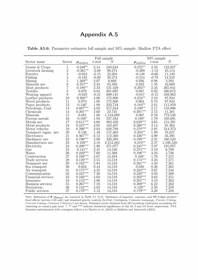
Appendix A.5
Table A5.6: Parameter estimates full sample and 50% sample: Shallow PTA effect
Full sample 50% sampleSector name Sector ρshallow t-stat N ρshallow t-stat N
Grains & Crops 1 0.249∗∗ 2.14 243,624 0.272∗∗ 2.33 122,027Livestock farming 2 -0.261∗∗ -2.08 90,274 -0.209 -1.53 45,114Forestry 3 -0.024 -0.15 22,304 -0.148 -0.66 11,140Fishing 4 -0.182 -0.80 28,274 -0.214 -0.78 14,218Mining 5 1.269∗∗ 2.07 6,669 0.936 0.98 3,292Minerals nec 6 0.357∗∗ 2.34 85,350 0.282 1.58 42,669Meat products 7 0.188∗∗ 2.33 531,429 0.203∗∗ 2.33 265,841Textiles 8 0.079 0.84 801,095 0.087 0.92 400,672Wearing apparel 9 -0.023 -0.21 699,145 -0.017 -0.15 349,963Leather products 10 0.208∗∗ 2.06 175,800 0.224∗∗ 2.10 87,824Wood products 11 0.073 1.00 175,800 0.063 0.73 87,824Paper products 12 0.146∗ 1.88 223,734 0.183∗∗ 2.01 111,859Petroleum, Coal 13 0.807∗∗∗ 4.02 317,824 0.530∗∗ 2.17 158,986Chemicals 14 0.201∗∗∗ 2.60 22,745 0.201∗∗∗ 2.72 11,281Minerals 15 0.081 1.00 1,544,089 0.067 0.76 772,538Ferrous metals 16 0.188∗ 1.94 337,582 0.189∗ 1.79 168,691Metals nec 17 0.611∗∗∗ 4.68 302,429 0.629∗∗∗ 4.65 151,291Metal products 18 0.247∗∗∗ 2.95 182,487 0.266∗∗∗ 3.14 91,364Motor vehicles 19 0.296∗∗∗ 3.04 628,789 0.278∗∗∗ 2.91 314,373Transport eqpm. nec 20 0.136 1.49 157,463 0.204∗∗ 1.99 78,827Electronics 21 0.467∗∗∗ 6.12 112,560 0.436∗∗∗ 4.90 56,295Machinery nec 22 0.196∗∗∗ 3.00 320,393 0.198∗∗∗ 2.91 160,523Manufactures nec 23 0.169∗∗ 2.10 2,212,282 0.219∗∗ 2.57 1,106,528Electricity 24 0.298∗∗∗ 5.96 371,077 0.245∗∗∗ 3.37 185,957Gas 25 0.141∗∗ 2.25 13,546 0.274∗∗∗ 3.19 6,789Water 26 0.229∗∗∗ 7.60 11,368 0.196∗∗∗ 4.33 5,726Construction 27 0.169∗∗∗ 2.67 14,434 0.168∗ 1.76 7,215Trade services 28 0.129∗∗∗ 3.55 14,518 0.174∗∗∗ 3.23 7,271Transport nec 29 0.182∗∗∗ 5.94 14,518 0.201∗∗∗ 4.50 7,261Sea transport 30 0.024 0.44 14,518 0.030 0.36 7,265Air transport 31 0.175∗∗∗ 4.35 14,518 0.224∗∗∗ 3.67 7,244Communication 32 0.221∗∗∗ 7.20 14,518 0.226∗∗∗ 4.93 7,269Financial services 33 0.160∗∗∗ 4.04 14,518 0.202∗∗∗ 3.62 7,251Insurance 34 0.152∗∗∗ 4.86 14,518 0.201∗∗∗ 4.10 7,263Business services 35 0.267∗∗∗ 7.58 14,518 0.309∗∗∗ 6.22 7,262Recreation 36 0.142∗∗∗ 4.02 14,518 0.129∗∗ 2.50 7,259Public services 37 0.178∗∗∗ 5.12 14,518 0.179∗∗∗ 3.20 7,250
Note: Estimates of θ (ρdeep) are reported in Table 5.1 (5.2). Estimates of importer, exporter, and HS 6-digit productfixed effects (sectors 1-23 only) and standard gravity controls (lnDist, Contiguity, Common Language, Former Colony,Current Colony, Common Colonizer) not shown. Standard errors obtained from 425 bootstrap replication accounting forclustering at country-pair level. *, ** and *** indicate statistical significance at the 10, 5 and 1% level, respectively. PTAdummies instrumented with contagion indices a la Martin et al. (2012) or Baldwin and Jaimovich (2012).

Chapter 5 241
Table A5.7: Welfare change, confidence intervals (α = .05), and bias: Non-TTIP coun-tries
(1) (2) (3) (4) (5) (6) (7) (8)
WN CIS CIBP1 CIBP1 CIBP2 Bias pwd(425, .05)symm. (eq.-t.) equal-tailed symm. equal-tailed abs. rel.
Country (in %) (in %) (in %) (in %) (in %) (in %pts.) (in %) (in %)
BEN 0.187 [0.133, 0.242] [0.154, 0.266] [0.125, 0.250] [0.108, 0.221] 0.008 4.230 0.132KGZ 0.177 [0.125, 0.230] [0.140, 0.250] [0.123, 0.231] [0.105, 0.214] 0.006 3.463 0.102XWF 0.156 [0.128, 0.184] [0.134, 0.190] [0.126, 0.186] [0.122, 0.178] 0.003 1.950 0.017TGO 0.149 [0.097, 0.200] [0.116, 0.215] [0.093, 0.205] [0.083, 0.181] 0.007 4.922 0.140ZWE 0.140 [0.115, 0.165] [0.119, 0.168] [0.115, 0.164] [0.111, 0.160] 0.002 1.203 0.016MDA 0.134 [0.069, 0.199] [0.094, 0.221] [0.065, 0.203] [0.047, 0.174] 0.008 5.854 0.256XSA 0.124 [0.102, 0.145] [0.107, 0.149] [0.102, 0.146] [0.099, 0.141] 0.002 1.282 0.013GIN 0.115 [0.086, 0.144] [0.093, 0.152] [0.084, 0.145] [0.078, 0.136] 0.004 3.724 0.027GEO 0.097 [0.059, 0.135] [0.073, 0.152] [0.057, 0.136] [0.042, 0.121] 0.004 4.207 0.115KEN 0.093 [0.072, 0.114] [0.077, 0.119] [0.072, 0.114] [0.067, 0.109] 0.002 2.534 0.019ECU 0.092 [0.045, 0.140] [0.056, 0.149] [0.045, 0.140] [0.036, 0.129] 0.002 1.714 0.118PAN 0.091 [0.065, 0.117] [0.070, 0.122] [0.067, 0.115] [0.060, 0.112] 0.002 1.974 0.041BWA 0.090 [0.024, 0.157] [0.027, 0.157] [0.025, 0.155] [0.023, 0.154] 0.001 1.236 0.172JOR 0.084 [0.054, 0.114] [0.064, 0.124] [0.054, 0.114] [0.044, 0.104] 0.004 4.586 0.094XOC 0.080 [0.064, 0.096] [0.068, 0.098] [0.063, 0.097] [0.062, 0.092] 0.002 2.030 0.010SEN 0.074 [0.046, 0.103] [0.058, 0.115] [0.043, 0.105] [0.034, 0.091] 0.004 5.894 0.109XNA 0.072 [0.040, 0.105] [0.045, 0.108] [0.039, 0.105] [0.036, 0.100] 0.003 4.474 0.052HKG 0.065 [0.047, 0.083] [0.050, 0.086] [0.047, 0.083] [0.043, 0.080] 0.002 2.725 0.021MUS 0.064 [0.047, 0.081] [0.051, 0.087] [0.048, 0.080] [0.041, 0.077] 0.002 3.115 0.022TZA 0.064 [0.048, 0.080] [0.052, 0.085] [0.048, 0.080] [0.043, 0.076] 0.002 2.979 0.022NPL 0.064 [0.049, 0.078] [0.053, 0.084] [0.049, 0.079] [0.043, 0.074] 0.002 3.017 0.017ARM 0.059 [0.034, 0.084] [0.042, 0.091] [0.033, 0.084] [0.027, 0.076] 0.003 4.623 0.070GHA 0.058 [0.042, 0.074] [0.045, 0.078] [0.042, 0.074] [0.038, 0.071] 0.002 2.851 0.020ALB 0.057 [0.030, 0.083] [0.042, 0.094] [0.028, 0.086] [0.020, 0.072] 0.003 5.205 0.114ETH 0.056 [0.041, 0.070] [0.045, 0.075] [0.041, 0.070] [0.036, 0.067] 0.002 3.382 0.021MAR 0.054 [0.030, 0.078] [0.040, 0.086] [0.028, 0.080] [0.022, 0.069] 0.003 5.530 0.094XER 0.050 [0.033, 0.066] [0.039, 0.073] [0.031, 0.068] [0.026, 0.060] 0.002 4.789 0.044LKA 0.047 [0.035, 0.059] [0.038, 0.062] [0.035, 0.059] [0.032, 0.056] 0.001 2.313 0.020EGY 0.042 [0.032, 0.052] [0.031, 0.051] [0.032, 0.053] [0.034, 0.054] -0.000 0.666 0.009NGA 0.041 [-0.008, 0.089] [-0.013, 0.092] [-0.010, 0.092] [-0.010, 0.094] -0.002 4.470 0.373UKR 0.039 [0.015, 0.064] [0.025, 0.072] [0.012, 0.066] [0.006, 0.053] 0.002 5.078 0.136PAK 0.039 [0.028, 0.050] [0.031, 0.052] [0.028, 0.050] [0.025, 0.047] 0.001 2.639 0.021XCB 0.037 [0.025, 0.049] [0.026, 0.049] [0.026, 0.049] [0.025, 0.048] -0.000 0.193 0.013LAO 0.036 [0.023, 0.048] [0.026, 0.051] [0.023, 0.048] [0.020, 0.045] 0.001 3.359 0.017VNM 0.035 [0.018, 0.051] [0.021, 0.056] [0.019, 0.050] [0.013, 0.049] 0.002 4.458 0.031BLR 0.034 [-0.002, 0.070] [0.008, 0.082] [-0.000, 0.067] [-0.015, 0.059] 0.002 5.515 0.311JAM 0.032 [0.016, 0.048] [0.018, 0.050] [0.016, 0.048] [0.014, 0.046] 0.001 3.375 0.032BGD 0.030 [0.016, 0.043] [0.018, 0.047] [0.017, 0.043] [0.013, 0.042] 0.001 1.908 0.032TUN 0.029 [0.015, 0.042] [0.018, 0.047] [0.015, 0.042] [0.010, 0.039] 0.001 3.719 0.037PRY 0.028 [0.012, 0.044] [0.010, 0.044] [0.011, 0.044] [0.012, 0.046] 0.000 0.462 0.034COL 0.028 [0.011, 0.045] [0.007, 0.041] [0.010, 0.045] [0.014, 0.048] -0.000 1.108 0.067PHL 0.027 [0.019, 0.035] [0.021, 0.038] [0.019, 0.035] [0.016, 0.033] 0.001 3.462 0.017ARE 0.026 [0.004, 0.048] [0.001, 0.047] [0.004, 0.049] [0.005, 0.051] 0.000 1.473 0.080GTM 0.026 [0.015, 0.037] [0.017, 0.040] [0.014, 0.037] [0.012, 0.034] 0.001 3.962 0.026UGA 0.025 [0.005, 0.046] [-0.000, 0.041] [0.006, 0.045] [0.010, 0.051] -0.000 1.801 0.091SLV 0.024 [0.013, 0.036] [0.016, 0.038] [0.013, 0.036] [0.011, 0.033] 0.001 4.237 0.026TUR 0.023 [0.010, 0.035] [0.014, 0.038] [0.010, 0.035] [0.007, 0.032] 0.001 4.745 0.051XSE 0.022 [0.018, 0.026] [0.018, 0.027] [0.018, 0.026] [0.017, 0.025] 0.000 1.373 0.003KHM 0.021 [-0.011, 0.053] [-0.012, 0.054] [-0.012, 0.054] [-0.012, 0.054] -0.001 5.034 0.186IND 0.020 [0.009, 0.031] [0.011, 0.032] [0.010, 0.031] [0.008, 0.029] 0.000 1.837 0.026XEF 0.018 [-0.009, 0.044] [-0.001, 0.056] [-0.008, 0.043] [-0.021, 0.036] 0.004 20.819 0.284URY 0.017 [0.012, 0.022] [0.013, 0.023] [0.012, 0.022] [0.011, 0.021] 0.000 1.965 0.006MWI 0.017 [-0.016, 0.049] [-0.025, 0.041] [-0.015, 0.049] [-0.007, 0.059] -0.001 5.422 0.364RWA 0.016 [0.003, 0.030] [-0.002, 0.025] [0.003, 0.030] [0.007, 0.035] -0.001 3.347 0.067MDG 0.015 [-0.003, 0.032] [-0.009, 0.027] [-0.003, 0.033] [0.003, 0.038] -0.001 5.083 0.130ISR 0.011 [-0.007, 0.030] [-0.003, 0.034] [-0.008, 0.031] [-0.011, 0.026] 0.001 11.712 0.159CMR 0.010 [-0.006, 0.025] [-0.009, 0.023] [-0.006, 0.026] [-0.003, 0.029] -0.001 8.065 0.102VEN 0.008 [-0.028, 0.045] [-0.043, 0.025] [-0.030, 0.047] [-0.009, 0.060] -0.004 45.613 1.773DOM 0.004 [-0.006, 0.014] [-0.006, 0.014] [-0.006, 0.014] [-0.006, 0.014] -0.000 10.833 0.103NZL 0.000 [-0.004, 0.005] [-0.004, 0.005] [-0.004, 0.005] [-0.005, 0.005] -0.000 28.479 0.253XWS -0.001 [-0.042, 0.040] [-0.053, 0.022] [-0.041, 0.039] [-0.024, 0.052] -0.003 287.308 17.011XEC -0.006 [-0.012, 0.000] [-0.014, -0.002] [-0.012, 0.001] [-0.010, 0.003] -0.000 7.763 0.032BLZ -0.006 [-0.048, 0.035] [-0.051, 0.034] [-0.049, 0.036] [-0.047, 0.039] -0.003 41.156 0.967
Note: pwd(B, t) denotes implied percentage deviation of bias estimate not exceed with probability (1− t)∗100 = 95% given B = 425bootstrap samples. pwd is calculated using the approximate method proposed by Cameron and Trivedi (2005), Ch. 11. Confidenceintervals in Columns (2)-(5) and bias estimate as defined in the text. Relative bias in percent of WN .

242 Parameter Uncertainty in NQTT Models
Welfare change, confidence intervals (α = .05), and bias: Non-TTIP countries, continued(1) (2) (3) (4) (5) (6) (7) (8)
WN CIS CIBP1 CIBP1 CIBP2 Bias pwd(425, .05)symm. (eq.-t.) equal-tailed symm. equal-tailed abs. rel.
Country (in %) (in %) (in %) (in %) (in %) (in %pts.) (in %) (in %)
BRA -0.007 [-0.009, -0.004] [-0.009, -0.004] [-0.009, -0.004] [-0.010, -0.004] 0.000 2.133 0.004XCF -0.008 [-0.091, 0.075] [-0.120, 0.047] [-0.089, 0.074] [-0.062, 0.105] -0.005 69.948 7.536XEA -0.008 [-0.026, 0.010] [-0.033, 0.004] [-0.028, 0.012] [-0.020, 0.016] -0.003 32.476 0.202MOZ -0.011 [-0.035, 0.012] [-0.035, 0.011] [-0.035, 0.012] [-0.034, 0.012] 0.002 17.646 0.184AUS -0.011 [-0.020, -0.003] [-0.021, -0.004] [-0.020, -0.003] [-0.019, -0.002] -0.000 0.135 0.025ARG -0.012 [-0.016, -0.007] [-0.018, -0.008] [-0.016, -0.007] [-0.015, -0.005] -0.000 2.234 0.011BOL -0.013 [-0.026, -0.000] [-0.029, -0.002] [-0.026, -0.001] [-0.024, 0.003] -0.000 1.396 0.048XTW -0.014 [-0.023, -0.005] [-0.025, -0.006] [-0.023, -0.005] [-0.023, -0.004] -0.000 1.035 0.025SGP -0.015 [-0.035, 0.005] [-0.035, 0.007] [-0.035, 0.005] [-0.036, 0.006] -0.000 1.263 0.099JPN -0.015 [-0.021, -0.009] [-0.021, -0.009] [-0.021, -0.010] [-0.021, -0.010] 0.000 0.243 0.010IDN -0.018 [-0.025, -0.010] [-0.026, -0.010] [-0.025, -0.010] [-0.025, -0.009] 0.000 0.255 0.011THA -0.022 [-0.031, -0.014] [-0.032, -0.015] [-0.031, -0.014] [-0.030, -0.013] -0.001 3.994 0.011CAN -0.024 [-0.046, -0.002] [-0.044, -0.000] [-0.046, -0.002] [-0.048, -0.004] 0.001 5.760 0.069NAM -0.025 [-0.045, -0.004] [-0.043, -0.004] [-0.044, -0.006] [-0.045, -0.006] 0.001 3.477 0.067ZAF -0.025 [-0.033, -0.017] [-0.032, -0.017] [-0.032, -0.018] [-0.033, -0.018] 0.001 2.897 0.008HND -0.030 [-0.048, -0.012] [-0.046, -0.009] [-0.048, -0.013] [-0.052, -0.014] -0.000 0.090 0.065CHN -0.031 [-0.038, -0.024] [-0.038, -0.024] [-0.037, -0.024] [-0.037, -0.023] -0.000 1.073 0.006CRI -0.032 [-0.051, -0.013] [-0.052, -0.015] [-0.051, -0.012] [-0.049, -0.011] -0.001 3.707 0.043XSC -0.033 [-0.057, -0.010] [-0.065, -0.016] [-0.057, -0.009] [-0.051, -0.002] -0.002 4.750 0.084CHE -0.033 [-0.051, -0.016] [-0.048, -0.015] [-0.049, -0.017] [-0.051, -0.018] 0.001 1.677 0.050KOR -0.038 [-0.050, -0.025] [-0.049, -0.025] [-0.050, -0.026] [-0.051, -0.026] 0.000 0.338 0.016NIC -0.041 [-0.066, -0.016] [-0.065, -0.016] [-0.065, -0.016] [-0.066, -0.016] -0.001 1.586 0.079MYS -0.042 [-0.058, -0.025] [-0.059, -0.027] [-0.058, -0.025] [-0.056, -0.024] -0.001 1.926 0.023BHR -0.045 [-0.083, -0.007] [-0.095, -0.017] [-0.082, -0.009] [-0.074, 0.005] -0.002 3.869 0.159MNG -0.047 [-0.061, -0.033] [-0.063, -0.034] [-0.062, -0.033] [-0.061, -0.031] 0.001 1.620 0.015NOR -0.050 [-0.170, 0.070] [-0.204, 0.020] [-0.169, 0.069] [-0.120, 0.104] -0.006 11.519 2.162XNF -0.052 [-0.148, 0.045] [-0.184, 0.004] [-0.145, 0.042] [-0.107, 0.080] -0.006 12.134 1.529XAC -0.054 [-0.136, 0.028] [-0.164, -0.002] [-0.134, 0.027] [-0.106, 0.056] -0.007 12.086 1.254XSU -0.057 [-0.106, -0.009] [-0.121, -0.024] [-0.108, -0.007] [-0.091, 0.006] -0.004 7.130 0.269CIV -0.058 [-0.086, -0.029] [-0.092, -0.036] [-0.086, -0.030] [-0.080, -0.023] -0.002 2.718 0.063IRN -0.071 [-0.113, -0.030] [-0.124, -0.042] [-0.115, -0.028] [-0.100, -0.018] -0.003 3.759 0.156XSM -0.075 [-0.106, -0.045] [-0.113, -0.048] [-0.106, -0.045] [-0.103, -0.038] 0.000 0.104 0.049PER -0.076 [-0.095, -0.056] [-0.097, -0.058] [-0.095, -0.057] [-0.094, -0.054] -0.000 0.133 0.018CHL -0.078 [-0.096, -0.059] [-0.098, -0.062] [-0.097, -0.059] [-0.094, -0.058] -0.000 0.168 0.016MEX -0.087 [-0.120, -0.053] [-0.120, -0.052] [-0.120, -0.053] [-0.122, -0.054] 0.002 2.129 0.043SAU -0.097 [-0.191, -0.003] [-0.228, -0.051] [-0.195, 0.001] [-0.142, 0.034] -0.008 7.789 0.879BFA -0.097 [-0.140, -0.054] [-0.147, -0.062] [-0.137, -0.057] [-0.132, -0.047] 0.001 0.908 0.074RUS -0.102 [-0.250, 0.046] [-0.303, -0.013] [-0.236, 0.032] [-0.191, 0.099] -0.008 8.154 1.654TWN -0.104 [-0.126, -0.083] [-0.128, -0.085] [-0.125, -0.083] [-0.124, -0.081] -0.002 1.705 0.016BRN -0.122 [-0.189, -0.056] [-0.215, -0.081] [-0.195, -0.049] [-0.163, -0.030] -0.006 4.705 0.261OMN -0.127 [-0.195, -0.058] [-0.217, -0.087] [-0.204, -0.050] [-0.166, -0.036] -0.006 4.941 0.296ZMB -0.162 [-0.204, -0.120] [-0.210, -0.126] [-0.205, -0.119] [-0.198, -0.113] -0.001 0.851 0.037KAZ -0.174 [-0.320, -0.027] [-0.371, -0.081] [-0.324, -0.023] [-0.266, 0.024] -0.009 4.961 0.874AZE -0.215 [-0.470, 0.039] [-0.580, -0.072] [-0.470, 0.039] [-0.359, 0.150] -0.018 8.403 2.411KWT -0.226 [-0.357, -0.095] [-0.408, -0.165] [-0.373, -0.080] [-0.288, -0.045] -0.015 6.448 0.789QAT -0.266 [-0.434, -0.098] [-0.488, -0.160] [-0.441, -0.092] [-0.373, -0.045] -0.011 4.077 0.735TTO -0.448 [-0.693, -0.204] [-0.768, -0.270] [-0.702, -0.195] [-0.627, -0.129] -0.009 2.052 0.612
Note: pwd(B, t) denotes implied percentage deviation of bias estimate not exceed with probability (1− t)∗100 = 95% given B = 425bootstrap samples. pwd is calculated using the approximate method proposed by Cameron and Trivedi (2005), Ch. 11. Confidenceintervals in Columns (2)-(5) and bias estimate as defined in the text. Relative bias in percent of WN .

Bibliography
Aichele, Rahel and Inga Heiland, “Where is the Value Added? Trade Liberalization andProduction Networks,” Technical Report, mimeo 2015.
Aizenman, Joshua, “Endogenous Pricing To Market and Financing Costs,” Journal ofMonetary Economics, 2004, 51 (4), 691–712.
Alessandria, George, Joseph P. Kaboski, and Virgiliu Midrigan, “Inventories, LumpyTrade, and Large Devaluations,” The American Economic Review, 2010, 100 (5), 2304–2339.
Alvarez, Fernando and Robert Jr. Lucas, “General Equilibrium Analysis of the Eaton-Kortum Model of International Trade,” Journal of Monetary Economics, 2007, 54 (6),1726–1768.
Amiti, Mary and Christopher A. Pissarides, “Trade and Industrial Location with Hetero-geneous Labor,” Journal of International Economics, 2005, 67 (2), 392–412.
Anderson, James E. and Eric van Wincoop, “Gravity with Gravitas: A Solution to theBorder Puzzle,” American Economic Review, 2003, 93 (1), 170–192.
and Yoto V. Yotov, “Terms of Trade and Global Efficiency Effects of Free TradeAgreements, 1990–2002,” Journal of International Economics, 2016, 99 (C), 279–298.
, Mario Larch, and Yoto V. Yotov, “On the Effects of the Transatlantic Trade andInvestment Partnership on Trade and Capital Accumulation,” Technical Report, BostonUniversity 2014.
Andrews, Donald W. K. and Moshe Buchinsky, “A Three-Step Method for Choosing theNumber of Bootstrap Repetitions,” Econometrica, 2000, 68 (1), 23–51.
Antrás, Pol and Davin Chor, “Organizing the Global Value Chain,” Econometrica, 2013,81 (6), 2127–2204.
Arkolakis, Costas, Arnaud Costinot, and Andres Rodríguez-Claire, “Gains From Tradeunder Monopolistic Competition: A Simple Example with Translog Expenditure Func-tions and Pareto Distributions of Firm-Level Productivity,” mimeo 2010.
, , and Andrés Rodríguez-Clare, “New Trade Models, Same Old Gains?,” AmericanEconomic Review, 2012, 102 (1), 94–130.

244 Bibliography
, , Dave Donaldson, and Andrés Rodríguez-Clare, “The Elusive Pro-CompetitiveEffects of Trade,” Working Paper 21370, National Bureau of Economic Research 2015.
Autor, David H., David Dorn, and Gordon H. Hanson, “The China Syndrome: LocalLabor Market Effects of Import Competition in the United States,” American EconomicReview, 2013, 103 (6), 2121–68.
Backus, David K. and Gregor W. Smith, “Consumption and Real Exchange Rates inDynamic Economies with Non-traded Goods,” Journal of International Economics,1993, 35 (3-4), 297 – 316.
Baldwin, Richard, “21st Century Regionalism: Filling the Gap between 21st CenturyTrade and 20th Century Trade Rules,” Technical Report, Center for Economic PolicyResearch 2011.
and Anthony J. Venables, “Spiders and Snakes: Offshoring and Agglomeration in theGlobal Economy,” Journal of International Economics, 2013, 90 (2), 245–254.
and Dany Jaimovich, “Are Free Trade Agreements Contagious?,” Journal of Interna-tional Economics, 2012, 88 (1), 1 – 16.
and Javier Lopez-Gonzalez, “Supply-chain Trade: A Portrait of Global Patterns andSeveral Testable Hypotheses,” The World Economy, 2015, 38 (11), 1682–1721.
Behrens, Kristian and Yasusada Murata, “Trade, Competition, and Efficiency,” Journalof International Economics, 2012, 87 (1), 1–17.
Beine, Michel, Frédéric Docquier, and Caglar Özden, “Diasporas,” Journal of DevelopmentEconomics, 2011, 95 (1), 30–41.
Bekaert, Geert, Campbell R. Harvey, Christian T. Lundblad, and Stephan Siegel, “WhatSegments Equity Markets?,” Review of Financial Studies, 2011, 24 (12), 3841–3890.
Belo, Frederico, “Production-based Measures of Risk for Asset Pricing,” Journal of Mon-etary Economics, 2010, 57 (2), 146 – 163.
Bems, Rudolfs and Robert C. Johnson, “Value-Added Exchange Rates,” NBER WorkingPaper No. 18498, National Bureau of Economic Research 2012.
, , and Kei-Mu Yi, “Vertical Linkages and the Collapse of Global Trade,” AmericanEconomic Review, Papers & Proceedings, 2011, 101 (3), 308–312.
Bénassy-Quéré, Agnès, Yvan Decreux, Lionel Fontagné, and David Khoudour-Casteras,“Economic Crisis and Global Supply Chains,” CEPII Working Paper No. 2009-15, Cen-tre d’Etudes Prospectives et d’Informations Internationales 2009.
Bergin, Paul R. and Robert C. Feenstra, “Staggered Price Setting and Endogenous Per-sistence,” Journal of Monetary Economics, 2000, 45 (3), 657–680.

Bibliography 245
Bergstrand, Jeffrey H., Peter Egger, and Mario Larch, “Gravity Redux: Estimation ofGravity-Equation Coefficients, Elasticities of Substitution, and General EquilibriumComparative Statics under Asymmetric Bilateral Trade Costs,” Journal of InternationalEconomics, 2013, 89 (1), 110–121.
Bilbiie, Florin O., Fabio Ghironi, and Marc J. Melitz, “Monopoly Power and EndogenousProduct Variety: Distortions and Remedies,” NBER Working Paper 14383 2008.
Black, Fischer, “Capital Market Equilibrium with Restricted Borrowing,” The Journal ofBusiness, 1972, 45 (3), 444–55.
Boldrin, Michele, Lawrence J. Christiano, and Jonas D. M. Fisher, “Habit Persistence,Asset Returns, and the Business Cycle,” The American Economic Review, 2001, 91 (1),149–166.
Caliendo, Lorenzo and Fernando Parro, “Estimates of the Trade and Welfare Effects ofNAFTA,” The Review of Economic Studies, 2015, 82 (1), 1–44.
Callen, Michael, Jean Imbs, and Paolo Mauro, “Pooling Risk among Countries,” Journalof International Economics, 2015, 96 (1), 88 – 99.
Cameron, A. C. and P. K. Trivedi, Microeconometrics: Methods and Applications, Cam-bridge University Press, New York, 2005.
Cameron, A. Colin, Jonah B. Gelbach, and Douglas L. Miller, “Robust Inference WithMultiway Clustering,” Journal of Business & Economic Statistics, 2011, 29 (2), 238–249.
Cipollina, Maria and Luca Salvatici, “Reciprocal Trade Agreements in Gravity Models:A Meta-Analysis,” Review of International Economics, 2010.
Cochrane, John H, “ Production-Based Asset Pricing and the Link between Stock Returnsand Economic Fluctuations,” Journal of Finance, 1991, 46 (1), 209–37.
, “A Cross-Sectional Test of an Investment-Based Asset Pricing Model,” Journal ofPolitical Economy, June 1996, 104 (3), 572–621.
Cochrane, John H., Asset Pricing, Princeton University Press, 2005.
Constantinides, George M., “Intertemporal Asset Pricing with Heterogeneous Consumersand Without Demand Aggregation,” Journal of Business, 1982, 2, 253–267.
Costinot, Arnaud and Andres Rodriguez-Clare, “Trade Theory with Numbers: Quanti-fying the Consequences of Globalization,” in Gita Gopinath, Elhanan Helpman, andKenneth Rogoff, eds., Handbook of International Economics, Vol. 4 2014, chapter 4,pp. 197–261.
and Jonathan Vogel, “Matching and Inequality in the World Economy,” Journal ofPolitical Economy, 2010, 118 (4), pp. 747–786.

246 Bibliography
, , and Su Wang, “An Elementary Theory of Global Supply Chains,” The Review ofEconomic Studies, 2013, 80 (1), 109–144.
Das, Sanghamitra, Mark J. Roberts, and James R. Tybout, “Market Entry Costs, Pro-ducer Heterogeneity, and Export Dynamics,” Econometrica, 2007, 75 (3), 837–873.
Daudin, Guillaume, Christine Rifflart, and Danielle Schweisguth, “Who Produces forWhom in the World Economy?,” Canadian Journal of Economics, 2011, 44 (4), 1403–1437.
Davidson, Carl, Fredrik Heyman, Steven Matusz, Fredrik Sjöholm, and Susan Chun Zhu,“Globalization and Imperfect Labor Market Sorting,” Journal of International Eco-nomics, 2014, 94 (2), 177 – 194.
, , , Fredrik Sjöholm, and Susan Chun Zhu, “Liberalized Trade and Worker-FirmMatching,” American Economic Review, 2012, 102 (3), 429–34.
, Steven J. Matusz, and Andrei Shevchenko, “Globalization and Firm Level Adjustmentwith Imperfect Labor Markets,” Journal of International Economics, 2008, 75 (2), 295–309.
Dekle, Robert, Jonathan Eaton, and Samuel Kortum, “Unbalanced Trade,” The AmericanEconomic Review, 2007, 97 (2), 351–355.
, , and , “Global Rebalancing with Gravity: Measuring the Burden of Adjustment,”IMF Staff Papers, 2008, 55 (3), 511–540.
di Giovanni, Julian and Andrei A. Levchenko, “Putting the Parts Together: Trade, VerticalLinkages, and Business Cycle Comovement,” American Economic Journal: Macroeco-nomics, 2010, 2 (2), 95–124.
di Giovanni, Julian, Andrei A. Levchenko, and Jing Zhang, “The Global Welfare Impactof China: Trade Integration and Technological Change,” American Economic Journal:Macroeconomics, 2014, 6 (3).
Dickstein, Michael J. and Eduardo Morales, “What do Exporters Know?,” Working Paper21351, National Bureau of Economic Research 2015.
Diewert, W. E., “Applications of Duality Theory,” in M. Intriligator and D. Kendrick,eds., Frontiers of Quantitative Economics, Vol. 2, North-Holland, 1974, pp. 106–171.
Dixit, Avinash K and Joseph E Stiglitz, “Monopolistic Competition and Optimum ProductDiversity,” American Economic Review, 1977, 67 (3), 297–308.
Djankov, Simeon, Caroline Freund, and Cong S. Pham, “Trading on Time,” The Reviewof Economics and Statistics, 2010, 92 (1), 166–173.
Docquier, F. and A. Marfouk, “International Migration by Educational Attainment (1990-2000) - Release 1.1,” in C. Özden and M. Schiff, eds., International Migration, Remit-tances and Development, Vol. 1, Palgrave Macmillan, New York, 2006, chapter 25.

Bibliography 247
Dür, Andreas, Leonardo Baccini, and Manfred Elsig, “The Design of International TradeAgreements: Introducing a New Database,” Review of International Organizations,2014, 9 (3), 353–375.
Dybvig, Philip H. and Jonathan E. Jr. Ingersoll, “Mean-Variance Theory in CompleteMarkets,” The Journal of Business, 1982, 55 (2), 233–251.
Eaton, Jonathan and Samuel Kortum, “Technology, Geography, and Trade,” Economet-rica, 2002, 70 (5), 1741–1779.
Eckel, Carsten, “Endogenous Sunk Costs, Flexible Manufacturing and the ProductivityEffects of International Trade,” Scandinavian Journal of Economics, 06 2009, 111 (2),369–386.
, “International Trade, Flexible Manufacturing, and Outsourcing,” Canadian Journalof Economics, 2009, 42 (4), 1449–1472.
Economides, Nicholas, “Symmetric Equilibrium Existence and Optimality in Differenti-ated Product Markets,” Journal of Economic Theory, 1989, 47 (1), 178–194.
Efron, Bradley, “Nonparametric Standard Errors and Confidence Intervals,” The Cana-dian Journal of Statistics / La Revue Canadienne de Statistique, 1981, 9 (2), 139–158.
, “Better Bootstrap Confidence Intervals,” Journal of the American Statistical Associa-tion, 1987, 82 (397), 171–185.
Egger, Harmut and Josef Falkinger, “International Trade and Financial Integration underTechnological Specialization and Uncertainty,” mimeo 2015.
Egger, Peter and Mario Larch, “An Assessment of the Europe Agreements’ Effects onBilateral Trade, GDP, and Welfare,” European Economic Review, 2011, 55 (2), 263–279.
, Joseph Francois, Miriam Manchin, and Douglas Nelson, “Non-Tariff Barriers, Integra-tion, and the Trans-Atlantic Economy,” Economic Policy, 2015, 30 (83).
, Mario Larch, and Kevin E Staub, “Trade Preferences and Bilateral Trade in Goodsand Services: A Structural Approach,” Technical Report, CEPR 2012.
, , Kevin E. Staub, and Rainer Winkelmann, “The Trade Effects of EndogenousPreferential Trade Agreements,” American Economic Journal: Economic Policy, 2011,3 (3), 113–43.
Fama, Eugene F., “Multiperiod Consumption-Investment Decisions,” The American Eco-nomic Review, 1970, 60 (1), 163–174.
and Kenneth R. French, “Common Risk Factors in the Returns on Stocks and Bonds,”Journal of Financial Economics, 1993, 33 (2), pp. 3–56.
and , “Size, Value, and Momentum in International Stock Returns,” Journal ofFinancial Economics, 2012, 105 (3), 457–472.
248 Bibliography
and , “A Five-factor Asset Pricing Model,” Journal of Financial Economics, 2015,116 (1), 1 – 22.
Fan, C. Simon and Oded Stark, “A Theory of Migration as Response to Economic Stigma,”International Economic Review, 2011, 52 (2), 549–571.
Feenstra, Robert C., “A Homothetic Utility Function for Monopolistic Competition Mod-els, without Constant Price Elasticity,” Economics Letters, 2003, 78 (1), 79–86.
and David E. Weinstein, “Globalization, Markups, and the U.S. Price Level,” NBERWorking Paper 15749 2010.
Felbermayr, Gabriel, Benedikt Heid, and Sybille Lehwald, “Transatlantic Free Trade:Winners, Losers, and Necessary Accompanying Measures,” Law and Business Reviewof the Americas, 2013, 19 (4), 445–484.
, , Mario Larch, and Erdal Yalcin, “Macroeconomic Potentials of Transatlantic FreeTrade: A High Resolution Perspective for Europe and the world,” Economic Policy,2015, 30 (83), 491–537.
, Volker Grossmann, and Wilhelm Kohler, “Chapter 18 - Migration, International Trade,and Capital Formation: Cause or Effect?,” in Barry R. Chiswick and Paul W. Miller,eds., Handbook of the Economics of International Migration, Vol. 1, North-Holland,2015, pp. 913 – 1025.
Fillat, José L. and Stefania Garetto, “Risk, Returns, and Multinational Production,” TheQuarterly Journal of Economics, 2015, 130 (4), 2027–2073.
, , and Lindsay Oldenski, “Diversification, Cost Structure, and the Risk Premium ofMultinational Corporations,” Journal of International Economics, 2015, 96 (1), 37–54.
Fitzgerald, Doireann, “Trade Costs, Asset Market Frictions, and Risk Sharing,” AmericanEconomic Review, 2012, 102 (6), 2700–2733.
Fontagne, Lionel, Julien Gourdon, and Sebastian Jean, “Transatlantic Trade: WhitherPartnership, Which Economic Consequences?,” Technical Report, CEPII 2013.
Francois, Joseph, Hans van Meijl, and Frank van Tongeren, “Trade liberalization in theDoha Development Round,” Economic Policy, 2005.
, Koen Berden, Saara Tamminen, Martin Thelle, and Paul Wymenga, “Nontariff Mea-sures in EU-US Trade and Investment – An Economic Analysis,” Technical Report 2009.Study commissioned by the European Commission, DG Trade, ECORYS NetherlandBV.
, Miriam Manchin, Hanna Norberg, Olga Pindyuk, and Patrick Tomberger, “ReducingTransatlantic Barriers to Trade and Investment. An Economic Assessment,” TechnicalReport, Centre for Economic Policy Research 2013.

Bibliography 249
Fukushima, Takashi, “Tariff Structure, Nontraded Goods and Theory of Piecemeal PolicyRecommendations,” International Economic Review, 1979, 20 (2), 427–35.
Ghosh, Madanmohan and Someshwar Rao, “Chinese Accession to the WTO: EconomicImplications for China, Other Asian and North American Economies,” Journal of PolicyModeling, 2010, 32 (3), 389–398.
Gomes, Joao F., Amir Yaron, and Lu Zhang, “Asset Prices and Business Cycles withCostly External Finance,” Review of Economic Dynamics, 2003, 6 (4), 767 – 788. Fi-nance and the Macroeconomy.
Graham, John and Campbell Harvey, “The Theory and Practice of Corporate Finance:Evidence from the Field,” Journal of Financial Economics, 2001, 60, 187–243.
Grossman, Gene M. and Assaf Razin, “International Capital Movements under Uncer-tainty,” Journal of Political Economy, 1984, 92 (2), 286–306.
and Elhanan Helpman, “Outsourcing in a Global Economy,” Review of EconomicStudies, 01 2005, 72 (1), 135–159.
and Esteban Rossi-Hansberg, “Trading Tasks: A Simple Theory of Offshoring,” Amer-ican Economic Review, 2008, 98 (5), 1978–97.
Hall, Peter, The Bootstrap and Edgeworth Expansion, Springer Verlag, New York, 1992.
Head, Keith and Thierry Mayer, “Gravity Equations: Workhorse,Toolkit, and Cookbook,”in G. Gopinath, E. Helpman, and K. Rogoff, eds., Handbook of International Economics,Vol. 4 2014, chapter 3, pp. 131–195.
Helpman, Elhanan, “International Trade in the Presence of Product Differentiation,Economies of Scale and Monopolistic Competition : A Chamberlin-Heckscher-OhlinApproach,” Journal of International Economics, 1981, 11 (3), 305–340.
, “Trade Patterns under Uncertainty with Country Specific Shocks,” Econometrica,1988, 56 (3), 645–659.
, “Trade, FDI, and the Organization of Firms,” Journal of Economic Literature, Septem-ber 2006, 44 (3), 589–630.
and Assaf Razin, “Uncertainty and International Trade in the Presence of Stock Mar-kets,” The Review of Economic Studies, 1978, 45 (2), 239–250.
, Oleg Itskhoki, and Stephen Redding, “Inequality and Unemployment in a GlobalEconomy,” Econometrica, 2010, 78 (4), 1239–1283.
Helsley, Robert W. and William C. Strange, “Matching and Agglomeration Economies ina System of Cities,” Regional Science and Urban Economics, 1990, 20 (2), 189–212.
Hertel, T.W., ed., Global Trade Analysis: Modeling and Applications, Cambridge Univer-sity Press, 1997.

250 Bibliography
Horowitz, Joel L., “The Bootstrap,” in J.J. Heckman and E.E. Leamer, eds., Handbook ofEconometrics, 1 ed., Vol. 5, Elsevier, 2001, chapter 52, pp. 3159–3228.
Hummels, David, Jun Ishii, and Kei-Mu Yi, “The Nature and Growth of Vertical Special-ization in World Trade,” Journal of International Economics, 2001.
Hummels, David L. and Georg Schaur, “Hedging Price Volatility Using Fast Transport,”Journal of International Economics, 2010, 82 (1), 15 – 25.
Jermann, Urban J., “Asset Pricing in Production Economies,” Journal of Monetary Eco-nomics, 1998, 41 (2), 257–275.
Johnson, Robert C. and Guillermo Noguera, “Accounting for intermediates: ProductionSharing and Trade in Value Added,” Journal of International Economics, 2012, 86 (2),224–236.
and , “Accounting for Intermediates: Production Sharing and Trade in value Added,”Journal of International Economics, 2012, 86 (2), 224–236.
and , “Fragmentation and Trade in Value Added over Four Decades,” NBERWorkingPaper No. 18186, National Bureau of Economic Research 2012.
and , “Proximity and Production Fragmentation,” American Economic Review, May2012, 102 (3), 407–411.
Keller, Wolfgang and Stephen Ross Yeaple, “The Gravity of Knowledge,” American Eco-nomic Review, 2013, 103 (4), 1414–44.
Khan, Aubhik and Julia K. Thomas, “Inventories and the Business Cycle: An EquilibriumAnalysis of (S, s) Policies,” The American Economic Review, 2007, 97 (4), 1165–1188.
Koopman, Robert, Zhi Wang, and Shang-Jin Wei, “Tracing Value-Added and DoubleCounting in Gross Exports,” American Economic Review, 2014, 104 (2), 459–94.
Kreickemeier, Udo and Jens Wrona, “Two-Way Migration between Similar Countries,”The World Economy, 2016, p. forthcoming.
Krugman, Paul, “Scale Economies, Product Differentiation, and the Pattern of Trade,”American Economic Review, December 1980, 70 (5), 950–59.
Krugman, Paul R., “Increasing Returns, Monopolistic Competition, and InternationalTrade,” Journal of International Economics, November 1979, 9 (4), 469–479.
Lai, Huiwen and Daniel Trefler, “The Gains from Trade with Monopolistic Competition:Specification, Estimation, and Mis-Specification,” Working Paper 9169, National Bu-reau of Economic Research 2002.
Lancaster, Kelvin J., “A New Approach to Consumer Theory,” The Journal of PoliticalEconomy, 1966, 74 (2), pp. 132–157.

Bibliography 251
Li, Qing, Maria Vassalou, and Yuhang Xing, “Sector Investment Growth Rates and theCross Section of Equity Returns,” The Journal of Business, 2006, 79 (3), 1637–1665.
Linden, Greg, Kenneth L. Kraemer, and Jason Dedrick, “Who Captures Value in a GlobalInnovation Network?: The Case of Apple’s iPod,” Communications of the ACM, 2009,52 (3), 140–144.
Lintner, John, The Review of Economics and Statistics.
Mankiw, N. Gregory and Michael D. Whinston, “Free Entry and Social Inefficiency,”RAND Journal of Economics, Spring 1986, 17 (1), 48–58.
Markusen, James R., “Factor Movements and Commodity Trade as Complements,” Jour-nal of International Economics, 1983, 14 (3-4), 341–356.
Martin, Philippe, Thierry Mayer, and Mathias Thoenig, “The Geography of Conflicts andRegional Trade Agreements,” American Economic Journal: Macroeconomics, 2012.
Mas-Colell, Andreu, Michael D. Whinston, and Jerry R. Green, Microeconomic Theory,New York, Oxford: Oxford University Press, 1995.
Mayda, Anna Maria, “International Migration: A Panel Data Analysis of the Determi-nants of Bilateral Flows,” Journal of Population Economics, 2010, 23 (4), 1249–1274.
Melitz, Marc J., “The Impact of Trade on Intra-Industry Reallocations and AggregateIndustry Productivity,” Econometrica, 2003, 71 (6), 1695–1725.
Morales, Eduardo, Gloria Sheu, and Andres Zahler, “Extended Gravity,” Working Paper21351, National Bureau of Economic Research 2015.
Mrázová, Monika and J. Peter Neary, “Not So Demanding: Preference Structure, Firm Be-havior, and Welfare,” University of Oxford, Department of Economics, Working Paper691, 2013.
and , “Together at Last: Trade Costs, Demand Structure, and Welfare,” AmericanEconomic Review, 2014, 104 (5), 298–303.
Noguera, Guillermo, “Trade Costs and Gravity for Gross and Value Added Trade,”manuscript, Columbia University 2012.
Obstfeld, Maurice and Kenneth Rogoff, “The Six Major Puzzles in International Macroeco-nomics: Is There a Common Cause?,” in “NBER Macroeconomics Annual 2000, Volume15,” MIT Press, 2001, pp. 339–412.
Ohnsorge, Franziska and Daniel Trefler, “Sorting It Out: International Trade and Pro-tection with Heterogeneous Workers,” Journal of Political Economy, 2007, 115 (5),868–892.
Ortega, Francesc and Giovanni Peri, “The effect of income and immigration policies oninternational migration,” Migration Studies, 2013, 1 (1), 47–74.

252 Bibliography
Ossa, Ralph, “Trade Wars and Trade Talks with Data,” American Economic Review, 2014,104 (12).
, “Quantitative Models in Commercial Policy,” Handbook of Commercial Policy, 2016,Forthcoming.
Pierce, J. and P. Schott, “Concording U.S. Harmonized System Codes over Time,” Journalof Official Statistics, 2012, 1, 53–68.
Rajan, Raghuram G. and Luigi Zingales, “Financial Dependence and Growth,” AmericanEconomic Review, 1998, 88 (3), 559–86.
Ramondo, Natalia and Veronica Rappoport, “The Role of Multinational Production in aRisky Environment,” Journal of International Economics, 2010, 81 (2), 240 – 252.
, , and Kim J. Ruhl, “The Proximity-Concentration Tradeoff under Uncertainty,” TheReview of Economic Studies, 2013.
Ravenstein, E.G., “The Laws of Migration,” Technical Report 2 1885.
Ródriguez-López, José Antonio, “Prices and Exchange Rates: A Theory of Disconnect,”The Review of Economic Studies, 2011.
Rowland, Patrick F. and Linda L. Tesar, “Multinationals and the Gains from InternationalDiversification,” Review of Economic Dynamics, 2004, 7 (4), 789 – 826.
Rubinstein, M., “An Aggregation Theorem for Securities Markets,” Journal of FinancialEconomics, 1974, 1, 225–44.
Salop, Steven C., “Monopolistic Competition with Outside Goods,” The Bell Journal ofEconomics, 1979, 10 (1), pp. 141–156.
Schmitt, Nicolas and Antoine Soubeyran, “A Simple Model of Brain Circulation,” Journalof International Economics, 2006, 69 (2), 296–309.
Shapiro, Joseph, “Trade Costs, CO2, and the Environment,” American Economic Journal:Economic Policy, fothcoming, 2015.
Sharpe, William F., “Capital Asset Prices: A Theory of Market Equilibrium under Con-ditions of Risk,” The Journal of Finance, 1964, 19 (3), 425–442.
Timmer, Marcel P., “The World Input-Output Database (WIOD): Contents, Sources andMethods,” WIOD working paper No. 10 2012.
Trefler, Daniel and Susan Chun Zhu, “The Structure of Factor Content Predictions,”Journal of International Economics, 2010.
Vickrey, William S., Simon P. Anderson, and Ralph M. Braid, “Spatial Competition,Monopolistic Competition, and Optimum Product Diversity,” International Journal ofIndustrial Organization, 1999, 17 (7), 953–963.

Bibliography 253
Vickrey, W.S., Microstatics, Harcourt, Brace and World, New York, 1964.
Vives, Xavier, Oligopoly Pricing: Old Ideas and New Tools, 1 ed., Vol. 1, The MIT Press,2001.
Vogel, Jonathan, “Spatial Competition with Heterogeneous Firms,” Journal of PoliticalEconomy, 2008, 116 (3), pp. 423–466.
Wang, Zhi, Shang-Jin Wei, and Kunfu Zhu, “Quantifying International Production Shar-ing at the Bilateral and Sector Levels,” Working Paper 19677, National Bureau ofEconomic Research November 2013.
Xing, Yuqing and Neal Detert, “How the iPhone Widens the United States Trade Deficitwith the People’s Republic of China,” ADBI Working Papers No. 257, Asian Develop-ment Bank Institute 2010.
Yi, Kei-Mu, “Can Vertical Specialization Explain the Growth of World Trade?,” Journalof Political Economy, 2003, 111 (1), 52–102.
, “Can Multistage Production Explain the Home Bias in Trade?,” The American Eco-nomic Review, 2010, 100 (1), 364–393.
Zhelobodko, Evgeny, Sergey Kokovin, Mathieu Parenti, and Jacques-François Thisse,“Monopolistic Competition: Beyond the Constant Elasticity of Substitution,” Econo-metrica, 2012, 80 (6), 2765–2784.


CURRICULUM VITAEInga Heiland
Born July 8th, 1986 in Ravensburg
10/2011 to present Junior Economistifo Institute - Leibniz Institute for Economic Researchat the University of Munich
Ph.D. Program in EconomicsMunich Graduate School of Economics,Ludwig-Maximilians-Universität, München
02/2015 to present Research AssistantDepartment of Economics,Eberhard Karls Universität Tübingen
10/2015 - 11/2015 Visiting ResearcherUniversity of Colorado, Boulder
01/2014 - 12/2014 Visiting ResearcherStanford University, Stanford
10/2009 - 06/2011 Studies in International Economics and Finance (M.Sc.)Eberhard Karls Universität, Tübingen andUniversity of Missouri, Columbia
10/2006 - 07/2009 Studies in International Economics (B.Sc.)Eberhard Karls Universität Tübingen
06/2005 AbiturFreie Waldorfschule Wangen, Wangen/Allgäu.