Embed Size (px)
Citation preview

Fixed-Bed Catalytic Reactors I
Copyright c© 2018 by Nob Hill Publishing, LLC
In a fixed-bed reactor the catalyst pellets are held in place and do not movewith respect to a fixed reference frame.
Material and energy balances are required for both the fluid, which occupiesthe interstitial region between catalyst particles, and the catalyst particles, inwhich the reactions occur.
The following figure presents several views of the fixed-bed reactor. Thespecies production rates in the bulk fluid are essentially zero. That is thereason we are using a catalyst.
1 / 160
Fixed-Bed Catalytic Reactors II
B
A cjs
D
C
cj
cj
T
R Tcj
Figure 7.1: Expanded views of a fixed-bed reactor.
2 / 160

The physical picture
Essentially all reaction occurs within the catalyst particles. The fluid in contactwith the external surface of the catalyst pellet is denoted with subscript s.
When we need to discuss both fluid and pellet concentrations andtemperatures, we use a tilde on the variables within the catalyst pellet.
3 / 160
The steps to consider
During any catalytic reaction the following steps occur:
1 transport of reactants and energy from the bulk fluid up to the catalyst pelletexterior surface,
2 transport of reactants and energy from the external surface into the porouspellet,
3 adsorption, chemical reaction, and desorption of products at the catalyticsites,
4 transport of products from the catalyst interior to the external surface of thepellet, and
5 transport of products into the bulk fluid.
The coupling of transport processes with chemical reaction can lead toconcentration and temperature gradients within the pellet, between the surfaceand the bulk, or both.
4 / 160

Some terminology and rate limiting steps
Usually one or at most two of the five steps are rate limiting and act toinfluence the overall rate of reaction in the pellet. The other steps areinherently faster than the slow step(s) and can accommodate any change inthe rate of the slow step.
The system is intraparticle transport controlled if step 2 is the slow process(sometimes referred to as diffusion limited).
For kinetic or reaction control, step 3 is the slowest process.
Finally, if step 1 is the slowest process, the reaction is said to be externallytransport controlled.
5 / 160
Effective catalyst properties
In this chapter, we model the system on the scale of Figure 7.1 C. Theproblem is solved for one pellet by averaging the microscopic processes thatoccur on the scale of level D over the volume of the pellet or over a solidsurface volume element.
This procedure requires an effective diffusion coefficient, Dj , to be identifiedthat contains information about the physical diffusion process and porestructure.
6 / 160
Catalyst Properties
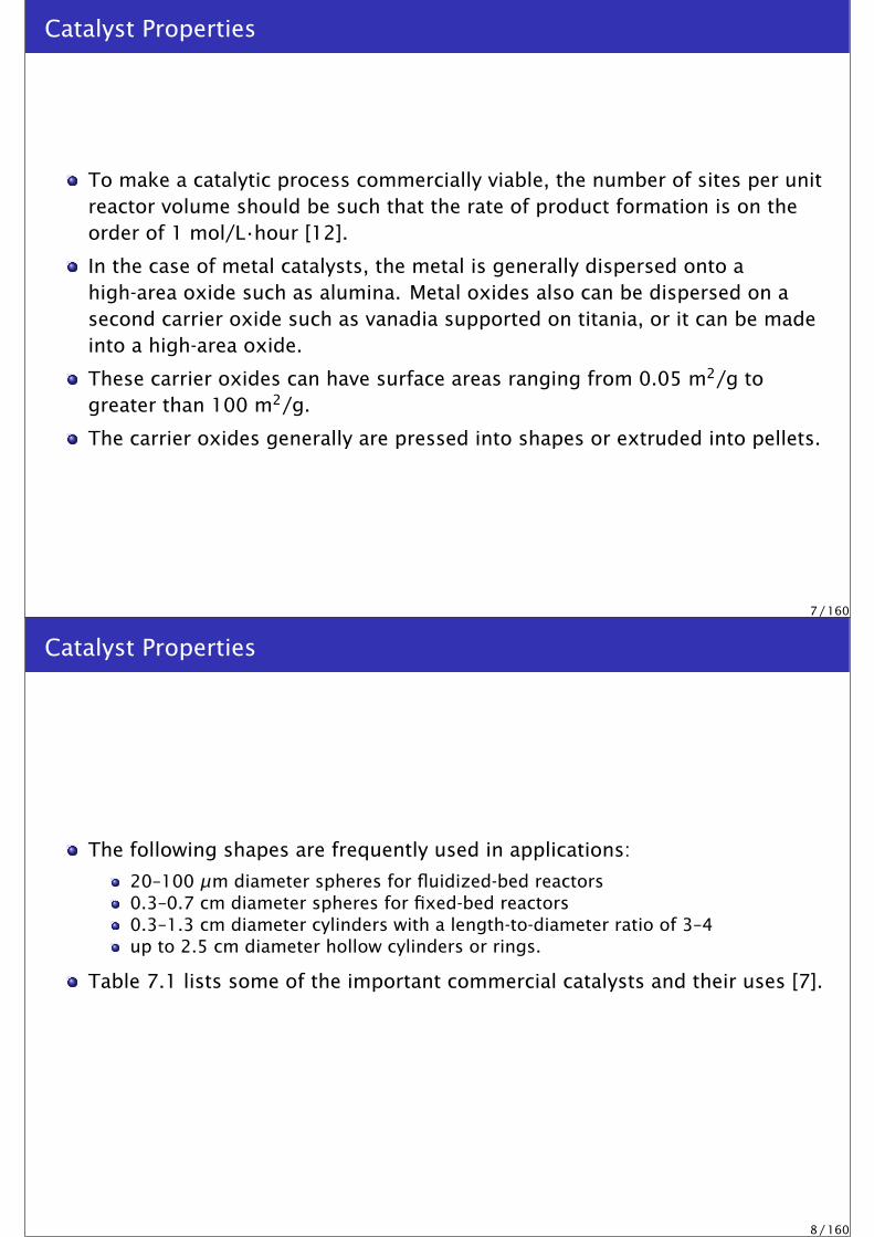
To make a catalytic process commercially viable, the number of sites per unitreactor volume should be such that the rate of product formation is on theorder of 1 mol/L·hour [12].
In the case of metal catalysts, the metal is generally dispersed onto ahigh-area oxide such as alumina. Metal oxides also can be dispersed on asecond carrier oxide such as vanadia supported on titania, or it can be madeinto a high-area oxide.
These carrier oxides can have surface areas ranging from 0.05 m2/g togreater than 100 m2/g.
The carrier oxides generally are pressed into shapes or extruded into pellets.
7 / 160
Catalyst Properties
The following shapes are frequently used in applications:
20–100 µm diameter spheres for fluidized-bed reactors0.3–0.7 cm diameter spheres for fixed-bed reactors0.3–1.3 cm diameter cylinders with a length-to-diameter ratio of 3–4up to 2.5 cm diameter hollow cylinders or rings.
Table 7.1 lists some of the important commercial catalysts and their uses [7].
8 / 160
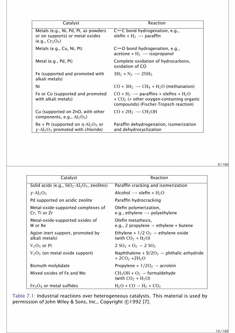
Catalyst Reaction
Metals (e.g., Ni, Pd, Pt, as powders C C bond hydrogenation, e.g.,or on supports) or metal oxides olefin + H2 -→ paraffin(e.g., Cr2O3)
Metals (e.g., Cu, Ni, Pt) C O bond hydrogenation, e.g.,acetone + H2 -→ isopropanol
Metal (e.g., Pd, Pt) Complete oxidation of hydrocarbons,oxidation of CO
Fe (supported and promoted with 3H2 + N2 -→ 2NH3alkali metals)
Ni CO + 3H2 -→ CH4 + H2O (methanation)
Fe or Co (supported and promoted CO + H2 -→ paraffins + olefins + H2Owith alkali metals) + CO2 (+ other oxygen-containing organic
compounds) (Fischer-Tropsch reaction)
Cu (supported on ZnO, with other CO + 2H2 -→ CH3OHcomponents, e.g., Al2O3)
Re + Pt (supported on η-Al2O3 or Paraffin dehydrogenation, isomerizationγ-Al2O3 promoted with chloride) and dehydrocyclization
9 / 160
Catalyst Reaction
Solid acids (e.g., SiO2-Al2O3, zeolites) Paraffin cracking and isomerization
γ-Al2O3 Alcohol -→ olefin + H2O
Pd supported on acidic zeolite Paraffin hydrocracking
Metal-oxide-supported complexes of Olefin polymerization,Cr, Ti or Zr e.g., ethylene -→ polyethylene
Metal-oxide-supported oxides of Olefin metathesis,W or Re e.g., 2 propylene → ethylene + butene
Ag(on inert support, promoted by Ethylene + 1/2 O2 → ethylene oxidealkali metals) (with CO2 + H2O)
V2O5 or Pt 2 SO2 + O2 → 2 SO3
V2O5 (on metal oxide support) Naphthalene + 9/2O2 → phthalic anhydride+ 2CO2 +2H2O
Bismuth molybdate Propylene + 1/2O2 → acrolein
Mixed oxides of Fe and Mo CH3OH + O2 → formaldehyde(with CO2 + H2O)
Fe3O4 or metal sulfides H2O + CO → H2 + CO2
Table 7.1: Industrial reactions over heterogeneous catalysts. This material is used bypermission of John Wiley & Sons, Inc., Copyright c©1992 [7].
10 / 160
Physical properties
Figure 7.1 D of shows a schematic representation of the cross section of asingle pellet.
The solid density is denoted ρs.
The pellet volume consists of both void and solid. The pellet void fraction (orporosity) is denoted by ε and
ε = ρpVg
in which ρp is the effective particle or pellet density and Vg is the pore volume.
The pore structure is a strong function of the preparation method, andcatalysts can have pore volumes (Vg) ranging from 0.1–1 cm3/g pellet.
11 / 160
Pore properties
The pores can be the same size or there can be a bimodal distribution withpores of two different sizes, a large size to facilitate transport and a smallsize to contain the active catalyst sites.
Pore sizes can be as small as molecular dimensions (several Angstroms) or aslarge as several millimeters.
Total catalyst area is generally determined using a physically adsorbedspecies, such as N2. The procedure was developed in the 1930s by Brunauer,Emmett and and Teller [5], and the isotherm they developed is referred to asthe BET isotherm.
12 / 160

B
A cjs
D
C
cj
cj
T
R Tcj
Figure: Expanded views of a fixed-bed reactor.
13 / 160
Effective Diffusivity
Catalyst ε τ100–110µm powder packed into a tube 0.416 1.56pelletized Cr2O3 supported on Al2O3 0.22 2.5pelletized boehmite alumina 0.34 2.7Girdler G-58 Pd on alumina 0.39 2.8Haldor-Topsøe MeOH synthesis catalyst 0.43 3.30.5% Pd on alumina 0.59 3.91.0% Pd on alumina 0.5 7.5pelletized Ag/8.5% Ca alloy 0.3 6.0pelletized Ag 0.3 10.0
Table 7.2: Porosity and tortuosity factors for diffusion in catalysts.
14 / 160

The General Balances in the Catalyst Particle
In this section we consider the mass and energy balances that arise with diffusionin the solid catalyst particle when considered at the scale of Figure 7.1 C.Consider the volume element depicted in the figure
e N j
E cj
15 / 160
Balances
Assume a fixed laboratory coordinate system in which the velocities are definedand let v j be the velocity of species j giving rise to molar flux N j
N j = cjv j , j = 1,2, . . . ,ns
Let E be the total energy within the volume element and e be the flux of totalenergy through the bounding surface due to all mechanisms of transport. Theconservation of mass and energy for the volume element implies
∂cj
∂t= −∇ ·N j + Rj , j = 1,2, . . . ,ns (7.10)
∂E∂t= −∇ · e
in which Rj accounts for the production of species j due to chemical reaction.
16 / 160

Fluxes
Next we consider the fluxes. Since we are considering the diffusion of mass in astationary, solid particle, we assume the mass flux is well approximated by
N j = −Dj∇cj , j = 1,2, . . . ,ns
in which Dj is an effective diffusivity for species j. We approximate the totalenergy flux by
e = −k∇T +∑
j
N jH j
This expression accounts for the transfer of heat by conduction, in which k is theeffective thermal conductivity of the solid, and transport of energy due to themass diffusion.
17 / 160
Steady state
In this chapter, we are concerned mostly with the steady state. Setting the timederivatives to zero and assuming constant thermodynamic properties produces
0 = Dj∇2cj + Rj , j = 1,2, . . . ,ns (7.14)
0 = k∇2T −∑
i
∆HRiri (7.15)
In multiple-reaction, noniosthermal problems, we must solve these equationsnumerically, so the assumption of constant transport and thermodynamicproperties is driven by the lack of data, and not analytical convenience.
18 / 160

Single Reaction in an Isothermal Particle
We start with the simplest cases and steadily remove restrictions and increasethe generality. We consider in this section a single reaction taking place in anisothermal particle.
First case: the spherical particle, first-order reaction, without externalmass-transfer resistance.
Next we consider other catalyst shapes, then other reaction orders, and thenother kinetic expressions such as the Hougen-Watson kinetics of Chapter 5.
We end the section by considering the effects of finite external mass transfer.
19 / 160
First-Order Reaction in a Spherical Particle
Ak-→ B, r = kcA
0 = Dj∇2cj + Rj , j = 1,2, . . . ,ns
Substituting the production rate into the mass balance, expressing the equation inspherical coordinates, and assuming pellet symmetry in θ and φ coordinates gives
DA1r2
ddr
(r2 dcA
dr
)− kcA = 0 (7.16)
in which DA is the effective diffusivity in the pellet for species A.
20 / 160

Units of rate constant
As written here, the first-order rate constant k has units of inverse time.Be aware that the units for a heterogeneous reaction rate constant are sometimesexpressed per mass or per area of catalyst.In these cases, the reaction rate expression includes the conversion factors,catalyst density or catalyst area, as illustrated in Example 7.1.
21 / 160
Boundary Conditions
We require two boundary conditions for Equation 7.16.
In this section we assume the concentration at the outer boundary of thepellet, cAs, is known
The symmetry of the spherical pellet implies the vanishing of the derivative atthe center of the pellet.
Therefore the two boundary conditions for Equation 7.16 are
cA = cAs , r = R
dcA
dr= 0 r = 0
22 / 160
Dimensionless form I
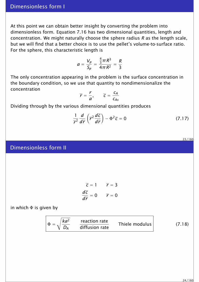
At this point we can obtain better insight by converting the problem intodimensionless form. Equation 7.16 has two dimensional quantities, length andconcentration. We might naturally choose the sphere radius R as the length scale,but we will find that a better choice is to use the pellet’s volume-to-surface ratio.For the sphere, this characteristic length is
a = Vp
Sp=
43πR3
4πR2= R
3
The only concentration appearing in the problem is the surface concentration inthe boundary condition, so we use that quantity to nondimensionalize theconcentration
r = ra, c = cA
cAs
Dividing through by the various dimensional quantities produces
1
r2
ddr
(r2 dc
dr
)− Φ2c = 0 (7.17)
23 / 160
Dimensionless form II
c = 1 r = 3
dcdr= 0 r = 0
in which Φ is given by
Φ =√
ka2
DA
reaction ratediffusion rate
Thiele modulus (7.18)
24 / 160

Thiele Modulus — Φ
The single dimensionless group appearing in the model is referred to as the Thielenumber or Thiele modulus in recognition of Thiele’s pioneering contribution inthis area [11].1 The Thiele modulus quantifies the ratio of the reaction rate to thediffusion rate in the pellet.
1In his original paper, Thiele used the term modulus to emphasize that this then unnameddimensionless group was positive. Later when Thiele’s name was assigned to this dimensionlessgroup, the term modulus was retained. Thiele number would seem a better choice, but the term Thielemodulus has become entrenched.
25 / 160
Solving the model
We now wish to solve Equation 7.17 with the given boundary conditions. Becausethe reaction is first order, the model is linear and we can derive an analyticalsolution.It is often convenient in spherical coordinates to consider the variabletransformation
c(r) = u(r)r
(7.20)
Substituting this relation into Equation 7.17 provides a simpler differentialequation for u(r),
d2u
dr2 − Φ2u = 0 (7.21)
with the transformed boundary conditions
u = 3 r = 3
u = 0 r = 0
The boundary condition u = 0 at r = 0 ensures that c is finite at the center of thepellet.
26 / 160
General solution – hyperbolic functions I
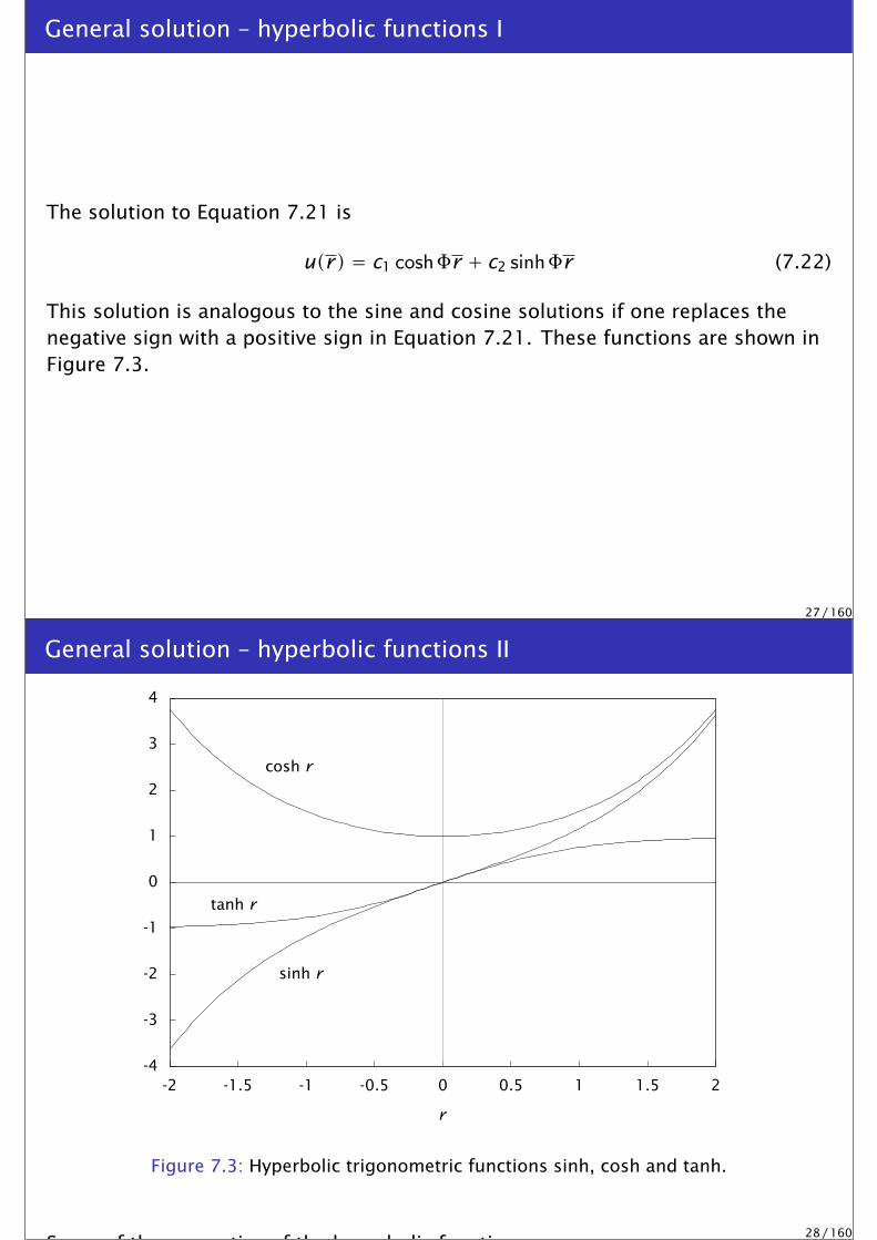
The solution to Equation 7.21 is
u(r) = c1 coshΦr + c2 sinhΦr (7.22)
This solution is analogous to the sine and cosine solutions if one replaces thenegative sign with a positive sign in Equation 7.21. These functions are shown inFigure 7.3.
27 / 160
General solution – hyperbolic functions II
-4
-3
-2
-1
0
1
2
3
4
-2 -1.5 -1 -0.5 0 0.5 1 1.5 2
sinh r
cosh r
tanh r
r
Figure 7.3: Hyperbolic trigonometric functions sinh, cosh and tanh.
Some of the properties of the hyperbolic functions are
cosh r = er + e−r
2d cosh r
dr= sinh r
sinh r = er − e−r
2d sinh r
dr= cosh r
tanh r = sinh rcosh r
28 / 160

Evaluating the unknown constants
The constants c1 and c2 are determined by the boundary conditions. SubstitutingEquation 7.22 into the boundary condition at r = 0 gives c1 = 0, and applying theboundary condition at r = 3 gives c2 = 3/ sinh3Φ.Substituting these results into Equations 7.22 and 7.20 gives the solution to themodel
c(r) = 3rsinhΦrsinh3Φ
(7.23)
29 / 160
Every picture tells a story
Figure 7.4 displays this solution for various values of the Thiele modulus.Note for small values of Thiele modulus, the reaction rate is small compared tothe diffusion rate, and the pellet concentration becomes nearly uniform. For largevalues of Thiele modulus, the reaction rate is large compared to the diffusion rate,and the reactant is converted to product before it can penetrate very far into thepellet.
30 / 160

0
0.2
0.4
0.6
0.8
1
0 0.5 1 1.5 2 2.5 3
Φ = 0.1
Φ = 0.5
Φ = 1.0
Φ = 2.0
c
r
Figure 7.4: Dimensionless concentration versus dimensionless radial position for differentvalues of the Thiele modulus.
31 / 160
Pellet total production rate
We now calculate the pellet’s overall production rate given this concentrationprofile. We can perform this calculation in two ways.The first and more direct method is to integrate the local production rate over thepellet volume. The second method is to use the fact that, at steady state, the rateof consumption of reactant within the pellet is equal to the rate at which materialfluxes through the pellet’s exterior surface.The two expressions are
RAp = 1Vp
∫ R
0RA(r)4πr2dr volume integral (7.24)
RAp = − Sp
VpDA
dcA
dr
∣∣∣∣r=R
surface flux(assumes steady state)
(7.25)
in which the local production rate is given by RA(r) = −kcA(r).We use the direct method here and leave the other method as an exercise.
32 / 160
Some integration
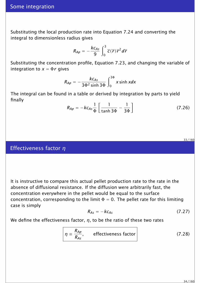
Substituting the local production rate into Equation 7.24 and converting theintegral to dimensionless radius gives
RAp = −kcAs
9
∫ 3
0c(r)r2dr
Substituting the concentration profile, Equation 7.23, and changing the variable ofintegration to x = Φr gives
RAp = − kcAs
3Φ2 sinh3Φ
∫ 3Φ
0x sinh xdx
The integral can be found in a table or derived by integration by parts to yieldfinally
RAp = −kcAs1Φ
[1
tanh3Φ− 1
3Φ
](7.26)
33 / 160
Effectiveness factor η
It is instructive to compare this actual pellet production rate to the rate in theabsence of diffusional resistance. If the diffusion were arbitrarily fast, theconcentration everywhere in the pellet would be equal to the surfaceconcentration, corresponding to the limit Φ = 0. The pellet rate for this limitingcase is simply
RAs = −kcAs (7.27)
We define the effectiveness factor, η, to be the ratio of these two rates
η ≡ RAp
RAs, effectiveness factor (7.28)
34 / 160
Effectiveness factor is the pellet production rate
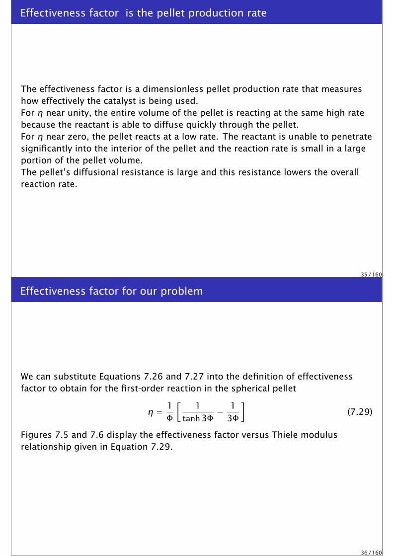
The effectiveness factor is a dimensionless pellet production rate that measureshow effectively the catalyst is being used.For η near unity, the entire volume of the pellet is reacting at the same high ratebecause the reactant is able to diffuse quickly through the pellet.For η near zero, the pellet reacts at a low rate. The reactant is unable to penetratesignificantly into the interior of the pellet and the reaction rate is small in a largeportion of the pellet volume.The pellet’s diffusional resistance is large and this resistance lowers the overallreaction rate.
35 / 160
Effectiveness factor for our problem
We can substitute Equations 7.26 and 7.27 into the definition of effectivenessfactor to obtain for the first-order reaction in the spherical pellet
η = 1Φ
[1
tanh3Φ− 1
3Φ
](7.29)
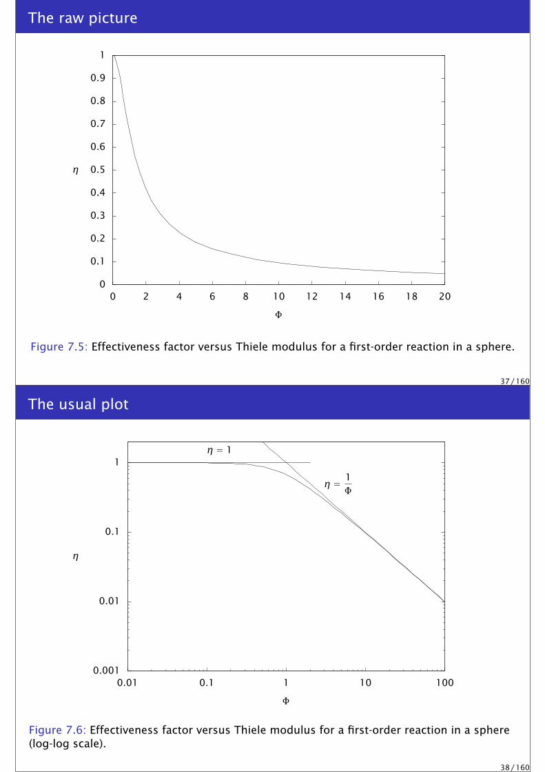
Figures 7.5 and 7.6 display the effectiveness factor versus Thiele modulusrelationship given in Equation 7.29.
36 / 160
The raw picture
0
0.1
0.2
0.3
0.4
0.5
0.6
0.7
0.8
0.9
1
0 2 4 6 8 10 12 14 16 18 20
η
Φ
Figure 7.5: Effectiveness factor versus Thiele modulus for a first-order reaction in a sphere.
37 / 160
The usual plot
0.001
0.01
0.1
1
0.01 0.1 1 10 100
η = 1Φ
η
η = 1
Φ
Figure 7.6: Effectiveness factor versus Thiele modulus for a first-order reaction in a sphere(log-log scale).
38 / 160
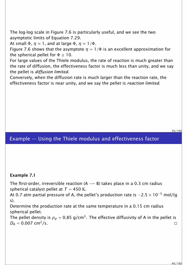
The log-log scale in Figure 7.6 is particularly useful, and we see the twoasymptotic limits of Equation 7.29.At small Φ, η ≈ 1, and at large Φ, η ≈ 1/Φ.Figure 7.6 shows that the asymptote η = 1/Φ is an excellent approximation forthe spherical pellet for Φ ≥ 10.For large values of the Thiele modulus, the rate of reaction is much greater thanthe rate of diffusion, the effectiveness factor is much less than unity, and we saythe pellet is diffusion limited.Conversely, when the diffusion rate is much larger than the reaction rate, theeffectiveness factor is near unity, and we say the pellet is reaction limited.
39 / 160
Example — Using the Thiele modulus and effectiveness factor
Example 7.1
The first-order, irreversible reaction (A -→ B) takes place in a 0.3 cm radiusspherical catalyst pellet at T = 450 K.At 0.7 atm partial pressure of A, the pellet’s production rate is −2.5× 10⁻⁵ mol/(gs).Determine the production rate at the same temperature in a 0.15 cm radiusspherical pellet.The pellet density is ρp = 0.85 g/cm3. The effective diffusivity of A in the pellet isDA = 0.007 cm2/s.
40 / 160
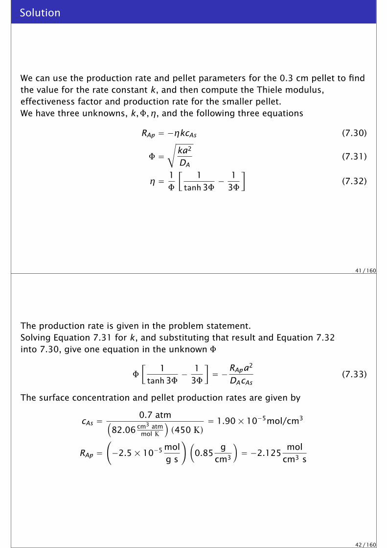
Solution
We can use the production rate and pellet parameters for the 0.3 cm pellet to findthe value for the rate constant k, and then compute the Thiele modulus,effectiveness factor and production rate for the smaller pellet.We have three unknowns, k,Φ, η, and the following three equations
RAp = −ηkcAs (7.30)
Φ =√
ka2
DA(7.31)
η = 1Φ
[1
tanh3Φ− 1
3Φ
](7.32)
41 / 160
The production rate is given in the problem statement.Solving Equation 7.31 for k, and substituting that result and Equation 7.32into 7.30, give one equation in the unknown Φ
Φ[
1tanh3Φ
− 13Φ
]= −RApa2
DAcAs(7.33)
The surface concentration and pellet production rates are given by
cAs = 0.7 atm(82.06 cm3 atm
mol K
)(450 K)
= 1.90× 10⁻⁵mol/cm3
RAp =(−2.5× 10⁻⁵ mol
g s
)(0.85
gcm3
)= −2.125
molcm3 s
42 / 160

Substituting these values into Equation 7.33 gives
Φ[
1tanh3Φ
− 13Φ
]= 1.60
This equation can be solved numerically yielding the Thiele modulus
Φ = 1.93
Using this result, Equation 7.31 gives the rate constant
k = 2.61 s−1
The smaller pellet is half the radius of the larger pellet, so the Thiele modulus ishalf as large or Φ = 0.964, which gives η = 0.685.
43 / 160
The production rate is therefore
RAp = −0.685(
2.6s−1)(
1.90× 10⁻⁵mol/cm3)= −3.38× 10⁻⁵ mol
cm3 s
We see that decreasing the pellet size increases the production rate by almost60%. Notice that this type of increase is possible only when the pellet is in thediffusion-limited regime.
44 / 160

Other Catalyst Shapes: Cylinders and Slabs
Here we consider the cylinder and slab geometries in addition to the spherecovered in the previous section.To have a simple analytical solution, we must neglect the end effects.We therefore consider in addition to the sphere of radius Rs, the semi-infinitecylinder of radius Rc , and the semi-infinite slab of thickness 2L, depicted inFigure 7.7.
45 / 160
Rs
Rc
L
a = Rc/2
a = L
a = Rs/3
Figure 7.7: Characteristic length a for sphere, semi-infinite cylinder and semi-infinite slab.
46 / 160

We can summarize the reaction-diffusion mass balance for these three geometriesby
DA1rq
ddr
(rq dcA
dr
)− kcA = 0 (7.34)
in whichq = 2 sphere
q = 1 cylinder
q = 0 slab
47 / 160
The associated boundary conditions are
cA = cAs
r = Rs spherer = Rc cylinderr = L slab
dcA
dr= 0 r = 0 all geometries
The characteristic length a is again best defined as the volume-to-surface ratio,which gives for these geometries
a = Rs
3sphere
a = Rc
2cylinder
a = L slab
48 / 160

The dimensionless form of Equation 7.34 is
1rq
ddr
(rq dc
dr
)− Φ2c = 0 (7.35)
c = 1 r = q + 1
dcdr= 0 r = 0
in which the boundary conditions for all three geometries can be compactlyexpressed in terms of q.
49 / 160
The effectiveness factor for the different geometries can be evaluated using theintegral and flux approaches, Equations 7.24–7.25, which lead to the twoexpressions
η = 1(q + 1)q
∫ q+1
0crqdr (7.36)
η = 1Φ2
dcdr
∣∣∣∣r=q+1
(7.37)
50 / 160
Effectiveness factor — Analytical
We have already solved Equations 7.35 and 7.36 (or 7.37) for the sphere, q = 2.Analytical solutions for the slab and cylinder geometries also can be derived. SeeExercise 7.1 for the slab geometry. The results are summarized in the followingtable.
Sphere η =1Φ
[1
tanh3Φ− 1
3Φ
](7.38)
Cylinder η =1Φ
I1(2Φ)I0(2Φ)
(7.39)
Slab η =tanhΦΦ
(7.40)
51 / 160
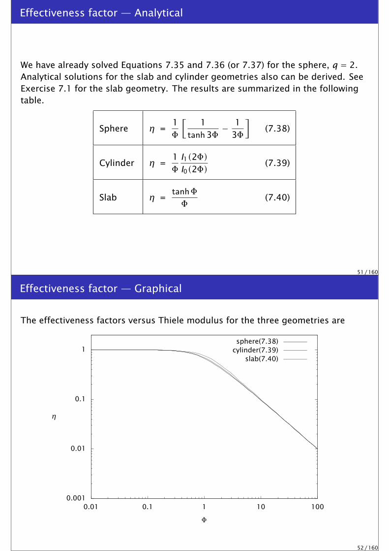
Effectiveness factor — Graphical
The effectiveness factors versus Thiele modulus for the three geometries are
0.001
0.01
0.1
1
0.01 0.1 1 10 100
η
Φ
sphere(7.38)cylinder(7.39)
slab(7.40)
52 / 160
Use the right Φ and ignore geometry!
Although the functional forms listed in the table appear quite different, we see inthe figure that these solutions are quite similar.The effectiveness factor for the slab is largest, the cylinder is intermediate, andthe sphere is the smallest at all values of Thiele modulus.The three curves have identical small Φ and large Φ asymptotes.The maximum difference between the effectiveness factors of the sphere and theslab η is about 16%, and occurs at Φ = 1.6. For Φ < 0.5 and Φ > 7, the differencebetween all three effectiveness factors is less than 5%.
53 / 160
Other Reaction Orders
For reactions other than first order, the reaction-diffusion equation is nonlinearand numerical solution is required.We will see, however, that many of the conclusions from the analysis of thefirst-order reaction case still apply for other reaction orders.We consider nth-order, irreversible reaction kinetics
Ak-→ B, r = kcn
A
The reaction-diffusion equation for this case is
DA1rq
ddr
(rq dcA
dr
)− kcn
A = 0 (7.41)
54 / 160

Thiele modulus for different reaction orders
The results for various reaction orders have a common asymptote if we insteaddefine
Φ =√
n + 12
kcn−1As a2
DA
Thiele modulusnth-order reaction
(7.42)
1rq
ddr
(rq dc
dr
)− 2
n + 1Φ2cn = 0
c = 1 r = q + 1
dcdr= 0 r = 0
η = 1(q + 1)q
∫ q+1
0cnrqdr
η = n + 12
1Φ2
dcdr
∣∣∣∣r=q+1
55 / 160
Reaction order greater than one
Figure 7.9 shows the effect of reaction order for n ≥ 1 in a spherical pellet.As the reaction order increases, the effectiveness factor decreases.Notice that the definition of Thiele modulus in Equation 7.42 has achieved thedesired goal of giving all reaction orders a common asymptote at high values of Φ.
56 / 160

Reaction order greater than one
0.1
1
0.1 1 10
η
Φ
n = 1n = 2n = 5n = 10
Figure 7.9: Effectiveness factor versus Thiele modulus in a spherical pellet; reaction ordersgreater than unity.
57 / 160
Reaction order less than one
Figure 7.10 shows the effectiveness factor versus Thiele modulus for reactionorders less than unity.Notice the discontinuity in slope of the effectiveness factor versus Thiele modulusthat occurs when the order is less than unity.
58 / 160

0.1
1
0.1 1 10
η
Φ
n = 0n = 1/4n = 1/2n = 3/4n = 1
Figure 7.10: Effectiveness factor versus Thiele modulus in a spherical pellet; reaction ordersless than unity.
59 / 160
Reaction order less than one I
Recall from the discussion in Chapter 4 that if the reaction order is less than unityin a batch reactor, the concentration of A reaches zero in finite time.In the reaction-diffusion problem in the pellet, the same kinetic effect causes thediscontinuity in η versus Φ.For large values of Thiele modulus, the diffusion is slow compared to reaction,and the A concentration reaches zero at some nonzero radius inside the pellet.For orders less than unity, an inner region of the pellet has identically zero Aconcentration.Figure 7.11 shows the reactant concentration versus radius for the zero-orderreaction case in a sphere at various values of Thiele modulus.
60 / 160

Reaction order less than one II
0
0.2
0.4
0.6
0.8
1
0 0.5 1 1.5 2 2.5 3
c
Φ = 0.4
Φ = 0.577
Φ = 0.8 Φ = 10
r
61 / 160
Reaction order less than one III
Figure 7.11: Dimensionless concentration versus radius for zero-order reaction (n = 0) in aspherical pellet (q = 2); for large Φ the inner region of the pellet has zero A concentration.
62 / 160
Use the right Φ and ignore reaction order!
Using the Thiele modulus
Φ =√
n + 12
kcn−1As a2
DA
allows us to approximate all orders with the analytical result derived for first order.The approximation is fairly accurate and we don’t have to solve the problemnumerically.
63 / 160
Hougen-Watson Kinetics
Given the discussion in Section 5.6 of adsorption and reactions on catalystsurfaces, it is reasonable to expect our best catalyst rate expressions may be ofthe Hougen-Watson form.Consider the following reaction and rate expression
A -→ products r = kcmKAcA
1+ KAcA
This expression arises when gas-phase A adsorbs onto the catalyst surface andthe reaction is first order in the adsorbed A concentration.
64 / 160

If we consider the slab catalyst geometry, the mass balance is
DAd2cA
dr2− kcm
KAcA
1+ KAcA= 0
and the boundary conditions are
cA = cAs r = L
dcA
dr= 0 r = 0
We would like to study the effectiveness factor for these kinetics.
65 / 160
First we define dimensionless concentration and length as before to arrive at thedimensionless reaction-diffusion model
d2c
dr2 − Φ2 c1+φc
= 0 (7.43)
c = 1 r = 1
dcdr= 0 r = 0 (7.44)
in which we now have two dimensionless groups
Φ =√
kcmKAa2
DA, φ = KAcAs (7.45)
66 / 160

We use the tilde to indicate Φ is a good first guess for a Thiele modulus for thisproblem, but we will find a better candidate subsequently.The new dimensionless group φ represents a dimensionless adsorption constant.The effectiveness factor is calculated from
η = RAp
RAs= −(Sp/Vp)DA dcA/dr|r=a
−kcmKAcAs/(1+ KAcAs)
which becomes upon definition of the dimensionless quantities
η = 1+φΦ2
dcdr
∣∣∣∣r=1
(7.46)
67 / 160
Rescaling the Thiele modulus
Now we wish to define a Thiele modulus so that η has a common asymptote atlarge Φ for all values of φ.This goal was accomplished for the nth-order reaction as shown in Figures 7.9and 7.10 by including the factor (n + 1)/2 in the definition of Φ given inEquation 7.42.The text shows how to do this analysis, which was developed independently byfour chemical engineers.
68 / 160

What did ChE professors work on in the 1960s?
This idea appears to have been discovered independently by three chemicalengineers in 1965.To quote from Aris [2, p. 113]
This is the essential idea in three papers published independently in March,May and June of 1965; see Bischoff [4], Aris [1] and Petersen [10]. A morelimited form was given as early as 1958 by Stewart in Bird, Stewart andLightfoot [3, p. 338].
69 / 160
Rescaling the Thiele modulus
The rescaling is accomplished by
Φ =(
φ1+φ
)1√
2 (φ− ln(1+φ)) Φ
So we have the following two dimensionless groups for this problem
Φ =(
φ1+φ
)√kcmKAa2
2DA (φ− ln(1+φ)) , φ = KAcAs (7.52)
The payoff for this analysis is shown in Figures 7.13 and 7.14.
70 / 160
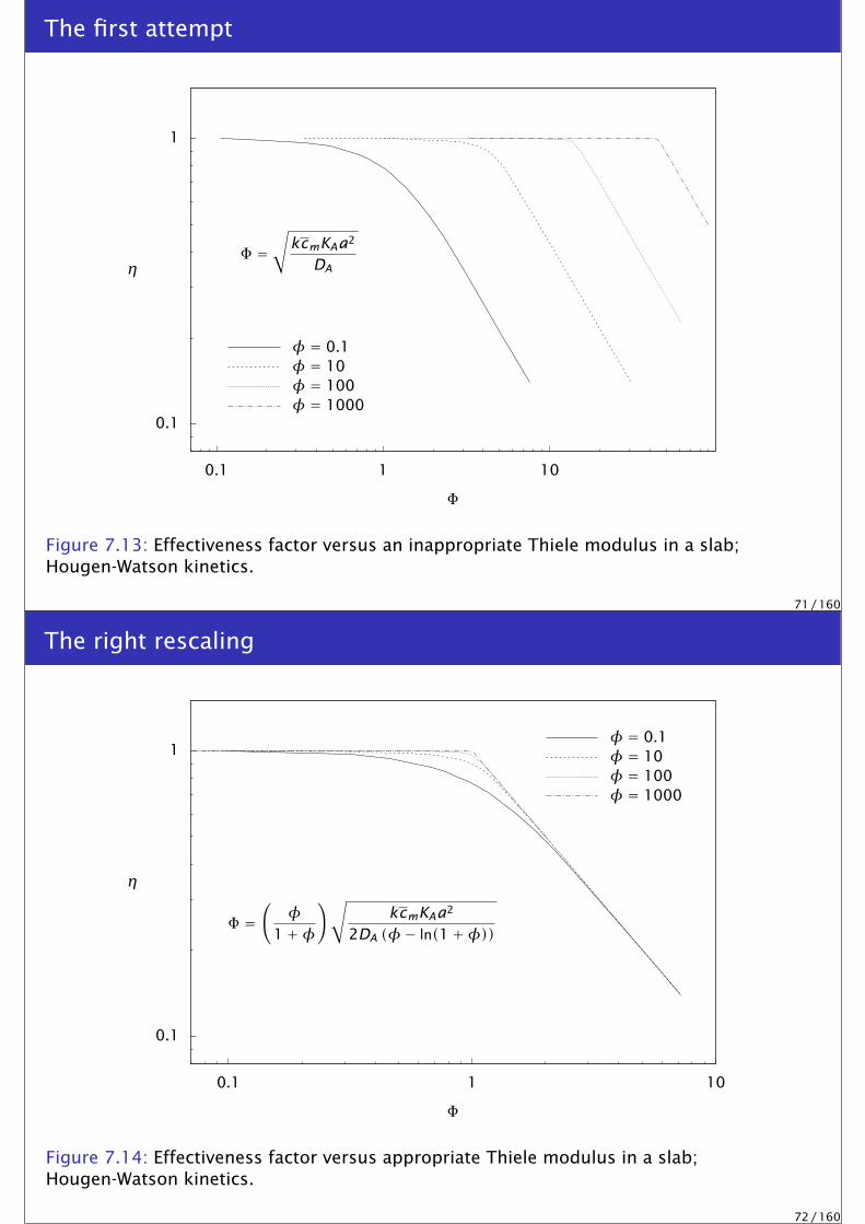
The first attempt
0.1
1
0.1 1 10
Φ =√
kcmKAa2
DAη
Φ
φ = 0.1φ = 10φ = 100φ = 1000
Figure 7.13: Effectiveness factor versus an inappropriate Thiele modulus in a slab;Hougen-Watson kinetics.
71 / 160
The right rescaling
0.1
1
0.1 1 10
Φ =(
φ1+φ
)√kcmKAa2
2DA (φ− ln(1+φ))
η
Φ
φ = 0.1φ = 10φ = 100φ = 1000
Figure 7.14: Effectiveness factor versus appropriate Thiele modulus in a slab;Hougen-Watson kinetics.
72 / 160

Use the right Φ and ignore the reaction form!
If we use our first guess for the Thiele modulus, Equation 7.45, we obtainFigure 7.13 in which the various values of φ have different asymptotes.Using the Thiele modulus defined in Equation 7.52, we obtain the results inFigure 7.14. Figure 7.14 displays things more clearly.Again we see that as long as we choose an appropriate Thiele modulus, we canapproximate the effectiveness factor for all values of φ with the first-orderreaction.The largest approximation error occurs near Φ = 1, and if Φ > 2 or Φ < 0.2, theapproximation error is negligible.
73 / 160
External Mass Transfer
If the mass-transfer rate from the bulk fluid to the exterior of the pellet is nothigh, then the boundary condition
cA(r = R) = cAf
is not satisfied.
0−R R
r
0−R R
r
cAf
cAs
cAf
cAcA
74 / 160

Mass transfer boundary condition
To obtain a simple model of the external mass transfer, we replace the boundarycondition above with a flux boundary condition
DAdcA
dr= km
(cAf − cA
), r = R (7.53)
in which km is the external mass-transfer coefficient.If we multiply Equation 7.53 by a/cAf DA, we obtain the dimensionless boundarycondition
dcdr= B (1− c) , r = 3 (7.54)
in which
B = kmaDA
(7.55)
is the Biot number or dimensionless mass-transfer coefficient.
75 / 160
Mass transfer model
Summarizing, for finite external mass transfer, the dimensionless model andboundary conditions are
1
r2
ddr
(r2 dc
dr
)− Φ2c = 0 (7.56)
dcdr= B (1− c) r = 3
dcdr= 0 r = 0
76 / 160

Solution
The solution to the differential equation satisfying the center boundary conditioncan be derived as in Section 7.4 to produce
c(r) = c2
rsinhΦr
in which c2 is the remaining unknown constant. Evaluating this constant using theexternal boundary condition gives
c(r) = 3r
sinhΦrsinh3Φ + (Φ cosh3Φ − (sinh3Φ)/3) /B
(7.57)
77 / 160
0
0.1
0.2
0.3
0.4
0.5
0.6
0.7
0.8
0.9
1
0 0.5 1 1.5 2 2.5 3
c
B = ∞
2.0
0.5
0.1
r
Figure 7.16: Dimensionless concentration versus radius for different values of the Biotnumber; first-order reaction in a spherical pellet with Φ = 1.
78 / 160

Effectiveness Factor
The effectiveness factor can again be derived by integrating the local reaction rateor computing the surface flux, and the result is
η = 1Φ
[1/ tanh3Φ − 1/(3Φ)
1+ Φ (1/ tanh3Φ − 1/(3Φ)) /B
](7.58)
in which
η = RAp
RAb
Notice we are comparing the pellet’s reaction rate to the rate that would beachieved if the pellet reacted at the bulk fluid concentration rather than the pelletexterior concentration as before.
79 / 160
10−5
10−4
10−3
10−2
10−1
100
0.01 0.1 1 10 100
B=∞
2.0
0.5
0.1
η
Φ
Figure 7.17: Effectiveness factor versus Thiele modulus for different values of the Biotnumber; first-order reaction in a spherical pellet.
80 / 160

Figure 7.17 shows the effect of the Biot number on the effectiveness factor or totalpellet reaction rate.Notice that the slope of the log-log plot of η versus Φ has a slope of negative tworather than negative one as in the case without external mass-transfer limitations(B = ∞).Figure 7.18 shows this effect in more detail.
81 / 160
10−6
10−5
10−4
10−3
10−2
10−1
100
10−2 10−1 100 101 102 103 104
B1 = 0.01
B2 = 100
√B1
√B2
η
Φ
Figure 7.18: Asymptotic behavior of the effectiveness factor versus Thiele modulus;first-order reaction in a spherical pellet.
82 / 160
Making a sketch of η versus Φ
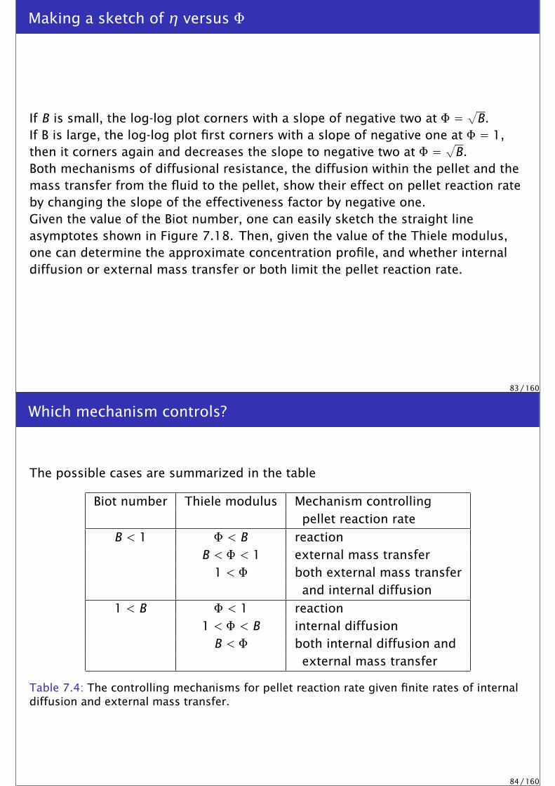
If B is small, the log-log plot corners with a slope of negative two at Φ = √B.If B is large, the log-log plot first corners with a slope of negative one at Φ = 1,then it corners again and decreases the slope to negative two at Φ = √B.Both mechanisms of diffusional resistance, the diffusion within the pellet and themass transfer from the fluid to the pellet, show their effect on pellet reaction rateby changing the slope of the effectiveness factor by negative one.Given the value of the Biot number, one can easily sketch the straight lineasymptotes shown in Figure 7.18. Then, given the value of the Thiele modulus,one can determine the approximate concentration profile, and whether internaldiffusion or external mass transfer or both limit the pellet reaction rate.
83 / 160
Which mechanism controls?
The possible cases are summarized in the table
Biot number Thiele modulus Mechanism controllingpellet reaction rate
B < 1 Φ < B reactionB < Φ < 1 external mass transfer
1 < Φ both external mass transferand internal diffusion
1 < B Φ < 1 reaction1 < Φ < B internal diffusion
B < Φ both internal diffusion andexternal mass transfer
Table 7.4: The controlling mechanisms for pellet reaction rate given finite rates of internaldiffusion and external mass transfer.
84 / 160

Observed versus Intrinsic Kinetic Parameters
We often need to determine a reaction order and rate constant for somecatalytic reaction of interest.
Assume the following nth-order reaction takes place in a catalyst particle
A -→ B, r1 = kcnA
We call the values of k and n the intrinsic rate constant and reaction order todistinguish them from what we may estimate from data.
The typical experiment is to change the value of cA in the bulk fluid, measurethe rate r1 as a function of cA, and then find the values of the parameters kand n that best fit the measurements.
85 / 160
Observed versus Intrinsic Kinetic Parameters
Here we show only that one should exercise caution with this estimation if we aremeasuring the rates with a solid catalyst. The effects of reaction, diffusion andexternal mass transfer may all manifest themselves in the measured rate.We express the reaction rate as
r1 = ηkcnAb (7.59)
We also know that at steady state, the rate is equal to the flux of A into thecatalyst particle
r1 = kmA(cAb − cAs) = DA
adcA
dr
∣∣∣∣r=R
(7.60)
We now study what happens to our experiment under different rate-limiting steps.
86 / 160

Reaction limited
First assume that both the external mass transfer and internal pellet diffusion arefast compared to the reaction. Then η = 1, and we would estimate the intrinsicparameters correctly in Equation 7.59
kob = k
nob = n
Everything goes according to plan when we are reaction limited.
87 / 160
Diffusion limited
Next assume that the external mass transfer and reaction are fast, but the internaldiffusion is slow. In this case we have η = 1/Φ, and using the definition of Thielemodulus and Equation 7.59
r1 = kobc(n+1)/2As (7.61)
kob = 1a
√2
n + 1DA
√k (7.62)
nob = (n + 1)/2 (7.63)
88 / 160

Diffusion limited
So we see two problems. The rate constant we estimate, kob, varies as the squareroot of the intrinsic rate constant, k. The diffusion has affected the measured rateof the reaction and disguised the rate constant.We even get an incorrect reaction order: a first-order reaction appears half-order,a second-order reaction appears first-order, and so on.
r1 = kobc(n+1)/2As
kob = 1a
√2
n + 1DA
√k
nob = (n + 1)/2
89 / 160
Diffusion limited
Also consider what happens if we vary the temperature and try to determine thereaction’s activation energy.Let the temperature dependence of the diffusivity, DA, be represented also inArrhenius form, with Ediff the activation energy of the diffusion coefficient.Let Erxn be the intrinsic activation energy of the reaction. The observed activationenergy from Equation 7.62 is
Eob = Ediff + Erxn
2
so both activation energies show up in our estimated activation energy.Normally the temperature dependence of the diffusivity is much smaller than thetemperature dependence of the reaction, Ediff Erxn, so we would estimate anactivation energy that is one-half the intrinsic value.
90 / 160

Mass transfer limited
Finally, assume the reaction and diffusion are fast compared to the external masstransfer. Then we have cAb cAs and Equation 7.60 gives
r1 = kmAcAb
If we vary cAb and measure r1, we would find the mass transfer coefficient insteadof the rate constant, and a first-order reaction instead of the true reaction order
kob = kmA
nob = 1
Normally, mass-transfer coefficients also have fairly small temperaturedependence compared to reaction rates, so the observed activation energy wouldbe almost zero, independent of the true reaction’s activation energy.
91 / 160
Moral to the story
Mass transfer and diffusion resistances disguise the reaction kinetics.We can solve this problem in two ways. First, we can arrange the experiment sothat mass transfer and diffusion are fast and do not affect the estimates of thekinetic parameters. How?If this approach is impractical or too expensive, we can alternatively model theeffects of the mass transfer and diffusion, and estimate the parameters DA andkmA simultaneously with k and n. We develop techniques in Chapter 9 to handlethis more complex estimation problem.
92 / 160

Nonisothermal Particle Considerations
We now consider situations in which the catalyst particle is not isothermal.
Given an exothermic reaction, for example, if the particle’s thermalconductivity is not large compared to the rate of heat release due to chemicalreaction, the temperature rises inside the particle.
We wish to explore the effects of this temperature rise on the catalystperformance.
93 / 160
Single, first-order reaction
We have already written the general mass and energy balances for the catalystparticle in Section 7.3.
0 = Dj∇2cj + Rj , j = 1,2, . . . ,ns
0 = k∇2T −∑
i
∆HRiri
Consider the single-reaction case, in which we have RA = −r andEquations 7.14 and 7.15 reduce to
DA∇2cA = r
k∇2T = ∆HRr
94 / 160

Reduce to one equation
We can eliminate the reaction term between the mass and energy balances toproduce
∇2T = ∆HRDA
k∇2cA
which relates the conversion of the reactant to the rise (or fall) in temperature.
Because we have assumed constant properties, we can integrate this equationtwice to give the relationship between temperature and A concentration
T − Ts = −∆HRDA
k(cAs − cA) (7.64)
95 / 160
Rate constant variation inside particle
We now consider a first-order reaction and assume the rate constant has anArrhenius form,
k(T ) = ks exp
[−E
(1T− 1
Ts
)]
in which Ts is the pellet exterior temperature, and we assume fast external masstransfer.Substituting Equation 7.64 into the rate constant expression gives
k(T ) = ks exp
[ETs
(1− Ts
Ts +∆HRDA(cA − cAs)/k
)]
96 / 160
Dimensionless parameters α, β, γ
We can simplify matters by defining three dimensionless variables
γ = ETs, β = −∆HRDAcAs
kTs, Φ2 = k(Ts)
DAa2
in which γ is a dimensionless activation energy, β is a dimensionless heat ofreaction, and Φ is the usual Thiele modulus. Again we use the tilde to indicate wewill find a better Thiele modulus subsequently.With these variables, we can express the rate constant as
k(T ) = ks exp
[γβ(1− c)
1+ β(1− c)
]
97 / 160
Nonisothermal model — Weisz-Hicks problem
We then substitute the rate constant into the mass balance, and assume aspherical particle to obtain the final dimensionless model
1
r2
ddr
(r2 dc
dr
)= Φ2c exp
(γβ(1− c)
1+ β(1− c)
)
dcdr= 0 r = 3
c = 1 r = 0 (7.65)
Equation 7.65 is sometimes called the Weisz-Hicks problem in honor of Weisz andHicks’s outstanding paper in which they computed accurate numerical solutions tothis problem [13].
98 / 160
Effectiveness factor for nonisothermal problem
Given the solution to Equation 7.65, we can compute the effectiveness factor forthe nonisothermal pellet using the usual relationship
η = 1Φ2
dcdr
∣∣∣∣r=3
If we perform the same asymptotic analysis of Section 7.4.4 on the Weisz-Hicksproblem, we find, however, that the appropriate Thiele modulus for this problem is
Φ = Φ/I(γ, β), I(γ, β) =[
2∫ 1
0c exp
(γβ(1− c)
1+ β(1− c)
)dc
]1/2
(7.66)
The normalizing integral I(γ, β) can be expressed as a sum of exponentialintegrals [2] or evaluated by quadrature.
99 / 160
10−1
100
101
102
103
10−4 10−3 10−2 10−1 100 101
β=0.60.4
0.3
0.2
0.1
β=0,−0.8
γ = 30
•
•
•
A
B
C
η
Φ
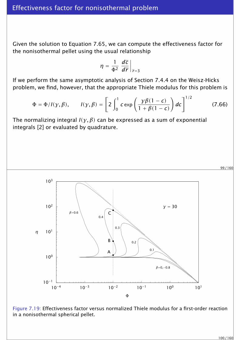
Figure 7.19: Effectiveness factor versus normalized Thiele modulus for a first-order reactionin a nonisothermal spherical pellet.
100 / 160

Note that Φ is well chosen in Equation 7.66 because the large Φ asymptotesare the same for all values of γ and β.
The first interesting feature of Figure 7.19 is that the effectiveness factor isgreater than unity for some values of the parameters.
Notice that feature is more pronounced as we increase the exothermic heat ofreaction.
For the highly exothermic case, the pellet’s interior temperature issignificantly higher than the exterior temperature Ts. The rate constant insidethe pellet is therefore much larger than the value at the exterior, ks. Thisleads to η greater than unity.
101 / 160
A second striking feature of the nonisothermal pellet is that multiple steadystates are possible.
Consider the case Φ = 0.01, β = 0.4 and γ = 30 shown in Figure 7.19.
The effectiveness factor has three possible values for this case.
We show in the next two figures the solution to Equation 7.65 for this case.
102 / 160

The concentration profile
0
0.2
0.4
0.6
0.8
1
1.2
0 0.5 1 1.5 2 2.5 3
c
C
B
A
γ = 30β = 0.4Φ = 0.01
r
103 / 160
And the temperature profile
0
0.1
0.2
0.3
0.4
0.5
0 0.5 1 1.5 2 2.5 3
T
A
B
C
γ = 30β = 0.4Φ = 0.01
r
104 / 160
MSS in nonisothermal pellet
The three temperature and concentration profiles correspond to an ignitedsteady state (C), an extinguished steady state (A), and an unstableintermediate steady state (B).
As we showed in Chapter 6, whether we achieve the ignited or extinguishedsteady state in the pellet depends on how the reactor is started.
For realistic values of the catalyst thermal conductivity, however, the pelletcan often be considered isothermal and the energy balance can beneglected [9].
Multiple steady-state solutions in the particle may still occur in practice,however, if there is a large external heat transfer resistance.
105 / 160
Multiple Reactions
As the next step up in complexity, we consider the case of multiple reactions.
Even numerical solution of some of these problems is challenging for tworeasons.
First, steep concentration profiles often occur for realistic parameter values,and we wish to compute these profiles accurately. It is not unusual for speciesconcentrations to change by 10 orders of magnitude within the pellet forrealistic reaction and diffusion rates.
Second, we are solving boundary-value problems because the boundaryconditions are provided at the center and exterior surface of the pellet.
We use the collocation method, which is described in more detail inAppendix A.
106 / 160
Multiple reaction example — Catalytic converter
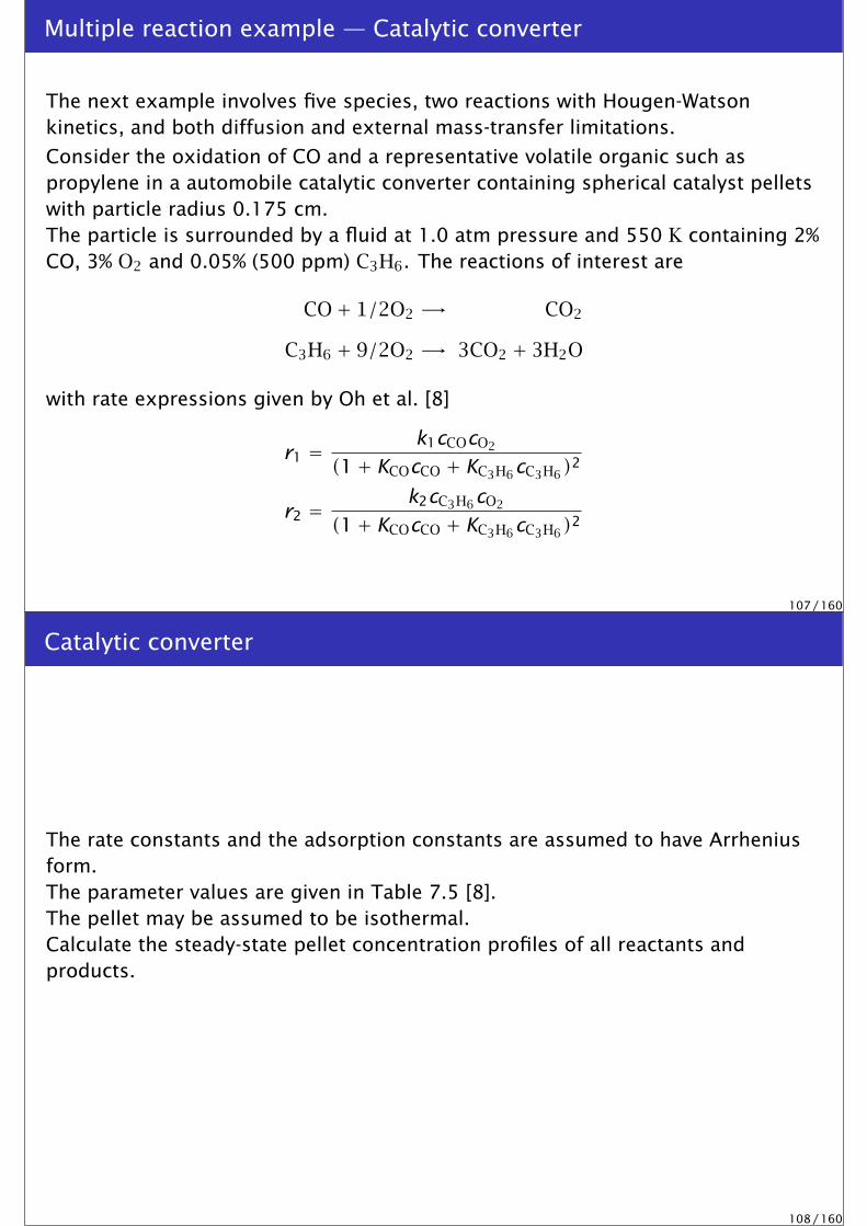
The next example involves five species, two reactions with Hougen-Watsonkinetics, and both diffusion and external mass-transfer limitations.
Consider the oxidation of CO and a representative volatile organic such aspropylene in a automobile catalytic converter containing spherical catalyst pelletswith particle radius 0.175 cm.The particle is surrounded by a fluid at 1.0 atm pressure and 550 K containing 2%CO, 3% O2 and 0.05% (500 ppm) C3H6. The reactions of interest are
CO+ 1/2O2 -→ CO2
C3H6 + 9/2O2 -→ 3CO2 + 3H2O
with rate expressions given by Oh et al. [8]
r1 =k1cCOcO2
(1+ KCOcCO + KC3H6 cC3H6)2
r2 =k2cC3H6 cO2
(1+ KCOcCO + KC3H6 cC3H6)2
107 / 160
Catalytic converter
The rate constants and the adsorption constants are assumed to have Arrheniusform.The parameter values are given in Table 7.5 [8].The pellet may be assumed to be isothermal.Calculate the steady-state pellet concentration profiles of all reactants andproducts.
108 / 160

Data
Parameter Value Units Parameter Value Units
P 1.013× 10⁵ N/m2 k10 7.07× 10¹⁹ mol/cm3· s
T 550 K k20 1.47× 10²¹ mol/cm3· s
R 0.175 cm KCO0 8.099× 106 cm3/mol
E1 13,108 K KC3H60 2.579× 108 cm3/mol
E2 15,109 K DCO 0.0487 cm2/s
ECO −409 K DO2 0.0469 cm2/s
EC3H6 191 K DC3H6 0.0487 cm2/s
cCOf 2.0 % kmCO 3.90 cm/s
cO2f 3.0 % kmO2 4.07 cm/s
cC3H6f 0.05 % kmC3H6 3.90 cm/s
Table 7.5: Kinetic and mass-transfer parameters for the catalytic converter example.
109 / 160
Solution
We solve the steady-state mass balances for the three reactant species,
Dj1r2
ddr
(r2 dcj
dr
)= −Rj
with the boundary conditions
dcj
dr= 0 r = 0
Djdcj
dr= kmj
(cjf − cj
)r = R
j = CO,O2,C3H6. The model is solved using the collocation method. Thereactant concentration profiles are shown in Figures 7.22 and 7.23.
110 / 160

0× 100
1× 10⁻⁷
2× 10⁻⁷
3× 10⁻⁷
4× 10⁻⁷
5× 10⁻⁷
6× 10⁻⁷
7× 10⁻⁷
0 0.02 0.04 0.06 0.08 0.1 0.12 0.14 0.16 0.18
O2
CO
C3H6
c(m
ol/
cm3)
r (cm)
Figure 7.22: Concentration profiles of reactants; fluid concentration of O2 (×), CO (+), C3H6(∗).
111 / 160
10−14
10−12
10−10
10−8
10−6
0 0.02 0.04 0.06 0.08 0.1 0.12 0.14 0.16 0.18
O2
CO
C3H6
c(m
ol/
cm3)
r (cm)
Figure 7.23: Concentration profiles of reactants (log scale); fluid concentration of O2 (×), CO(+), C3H6 (∗).
112 / 160
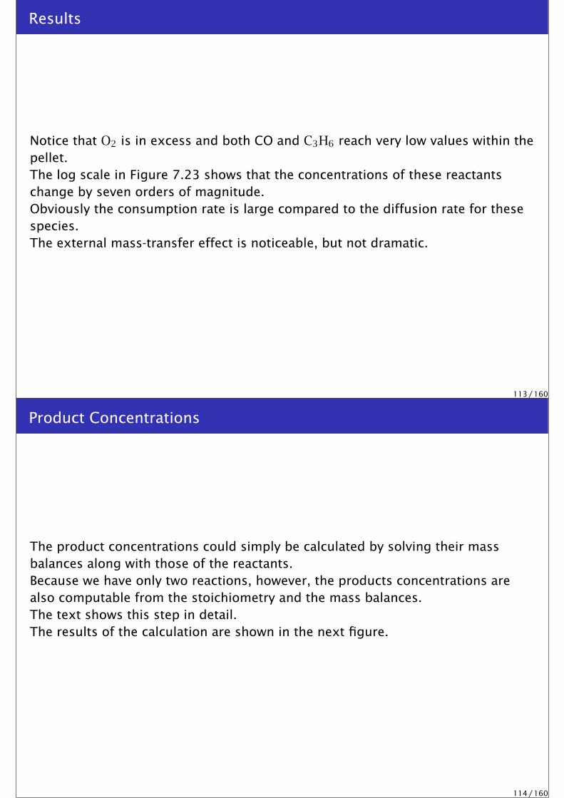
Results
Notice that O2 is in excess and both CO and C3H6 reach very low values within thepellet.The log scale in Figure 7.23 shows that the concentrations of these reactantschange by seven orders of magnitude.Obviously the consumption rate is large compared to the diffusion rate for thesespecies.The external mass-transfer effect is noticeable, but not dramatic.
113 / 160
Product Concentrations
The product concentrations could simply be calculated by solving their massbalances along with those of the reactants.Because we have only two reactions, however, the products concentrations arealso computable from the stoichiometry and the mass balances.The text shows this step in detail.The results of the calculation are shown in the next figure.
114 / 160
0× 100
1× 10⁻⁷
2× 10⁻⁷
3× 10⁻⁷
4× 10⁻⁷
5× 10⁻⁷
0 0.02 0.04 0.06 0.08 0.1 0.12 0.14 0.16 0.18
CO2
H2O
c(m
ol/
cm3)
r (cm)
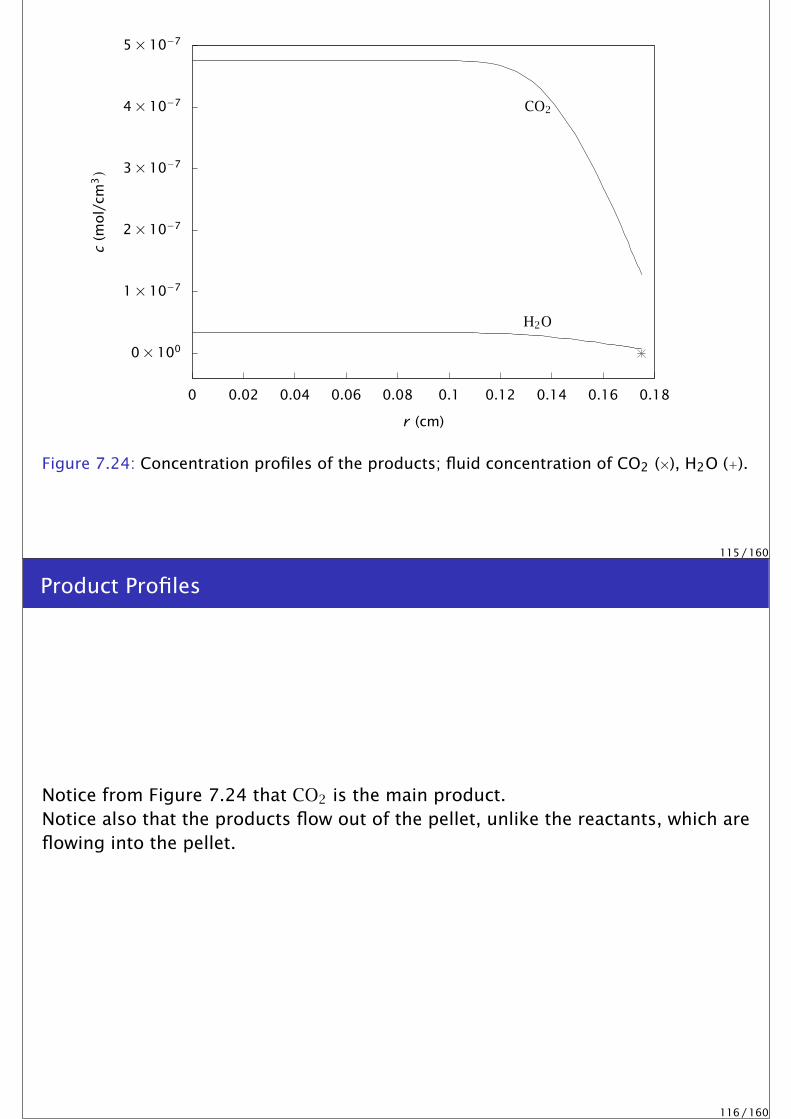
Figure 7.24: Concentration profiles of the products; fluid concentration of CO2 (×), H2O (+).
115 / 160
Product Profiles
Notice from Figure 7.24 that CO2 is the main product.Notice also that the products flow out of the pellet, unlike the reactants, which areflowing into the pellet.
116 / 160

Fixed-Bed Reactor Design
Given our detailed understanding of the behavior of a single catalyst particle,we now are prepared to pack a tube with a bed of these particles and solvethe fixed-bed reactor design problem.
In the fixed-bed reactor, we keep track of two phases. The fluid-phasestreams through the bed and transports the reactants and products throughthe reactor.
The reaction-diffusion processes take place in the solid-phase catalystparticles.
The two phases communicate to each other by exchanging mass and energyat the catalyst particle exterior surfaces.
We have constructed a detailed understanding of all these events, and now weassemble them together.
117 / 160
Coupling the Catalyst and Fluid
We make the following assumptions:
1 Uniform catalyst pellet exterior. Particles are small compared to the length ofthe reactor.
2 Plug flow in the bed, no radial profiles.
3 Neglect axial diffusion in the bed.
4 Steady state.
118 / 160

Fluid phase
In the fluid phase, we track the molar flows of all species, the temperature and thepressure.We can no longer neglect the pressure drop in the tube because of the catalystbed. We use an empirical correlation to describe the pressure drop in a packedtube, the well-known Ergun equation [6].
dNj
dV= Rj (7.67)
QρCpdTdV= −
∑
i
∆HRiri + 2R
Uo(Ta − T )
dPdV= − (1− εB)
Dpε3B
Q
A2c
[150
(1− εB)µf
Dp+ 7
4ρQAc
]
The fluid-phase boundary conditions are provided by the known feed conditions atthe tube entrance
Nj = Njf , z = 0
T = Tf , z = 0
P = Pf , z = 0
119 / 160
Catalyst particle
Inside the catalyst particle, we track the concentrations of all species and thetemperature.
Dj1r2
ddr
(r2 dc j
dr
)= −Rj
k1r2
ddr
(r2 dT
dr
)=∑
i
∆HRi r i
The boundary conditions are provided by the mass-transfer and heat-transfer ratesat the pellet exterior surface, and the zero slope conditions at the pellet center
dc j
dr= 0 r = 0
Djdc j
dr= kmj(cj − c j) r = R
dTdr= 0 r = 0
kdTdr= kT (T − T ) r = R
120 / 160
Coupling equations
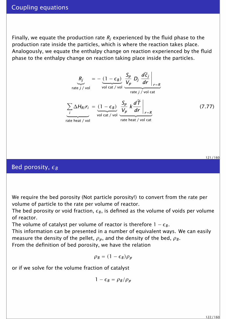
Finally, we equate the production rate Rj experienced by the fluid phase to theproduction rate inside the particles, which is where the reaction takes place.Analogously, we equate the enthalpy change on reaction experienced by the fluidphase to the enthalpy change on reaction taking place inside the particles.
Rj︸︷︷︸rate j / vol
= − (1− εB)︸ ︷︷ ︸vol cat / vol
Sp
VpDj
dc j
dr
∣∣∣∣∣r=R︸ ︷︷ ︸
rate j / vol cat
∑
i
∆HRiri
︸ ︷︷ ︸rate heat / vol
= (1− εB)︸ ︷︷ ︸vol cat / vol
Sp
Vpk
dTdr
∣∣∣∣∣r=R︸ ︷︷ ︸
rate heat / vol cat
(7.77)
121 / 160
Bed porosity, εB
We require the bed porosity (Not particle porosity!) to convert from the rate pervolume of particle to the rate per volume of reactor.The bed porosity or void fraction, εB , is defined as the volume of voids per volumeof reactor.The volume of catalyst per volume of reactor is therefore 1− εB .This information can be presented in a number of equivalent ways. We can easilymeasure the density of the pellet, ρp, and the density of the bed, ρB .From the definition of bed porosity, we have the relation
ρB = (1− εB)ρp
or if we solve for the volume fraction of catalyst
1− εB = ρB/ρp
122 / 160

In pictures
Rj
r i
Rj
ri
Mass
Rj = (1− εB)Rjp
Rjp = −Sp
VpDj
dcj
dr
∣∣∣∣∣r=R
Energy∑
i
∆HRi ri = (1− εB)∑
i
∆HRi r ip
∑
i
∆HRi r ip =Sp
Vpk
dTdr
∣∣∣∣∣r=R
Figure 7.25: Fixed-bed reactor volume element containing fluid and catalyst particles; theequations show the coupling between the catalyst particle balances and the overall reactorbalances.
123 / 160
Summary
Equations 7.67–7.77 provide the full packed-bed reactor model given ourassumptions.We next examine several packed-bed reactor problems that can be solved withoutsolving this full set of equations.Finally, we present an example that requires numerical solution of the full set ofequations.
124 / 160
First-order, isothermal fixed-bed reactor
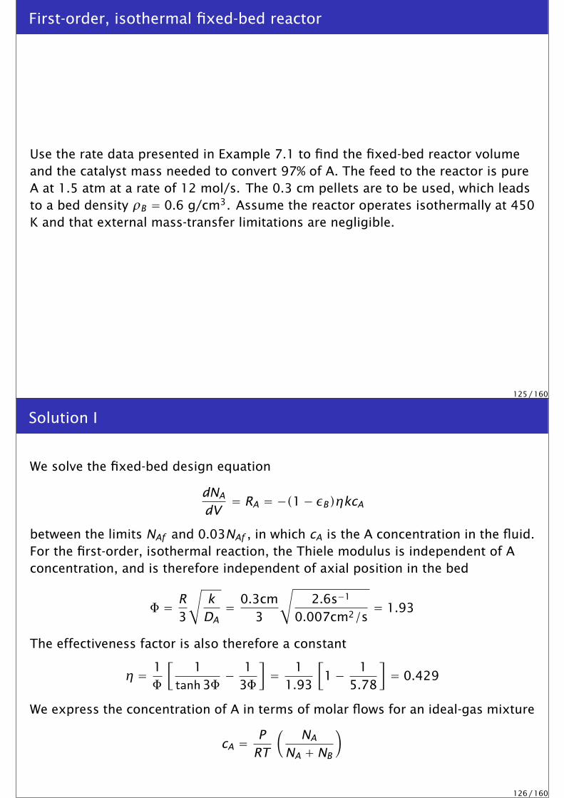
Use the rate data presented in Example 7.1 to find the fixed-bed reactor volumeand the catalyst mass needed to convert 97% of A. The feed to the reactor is pureA at 1.5 atm at a rate of 12 mol/s. The 0.3 cm pellets are to be used, which leadsto a bed density ρB = 0.6 g/cm3. Assume the reactor operates isothermally at 450K and that external mass-transfer limitations are negligible.
125 / 160
Solution I
We solve the fixed-bed design equation
dNA
dV= RA = −(1− εB)ηkcA
between the limits NAf and 0.03NAf , in which cA is the A concentration in the fluid.For the first-order, isothermal reaction, the Thiele modulus is independent of Aconcentration, and is therefore independent of axial position in the bed
Φ = R3
√k
DA= 0.3cm
3
√2.6s−1
0.007cm2/s= 1.93
The effectiveness factor is also therefore a constant
η = 1Φ
[1
tanh3Φ− 1
3Φ
]= 1
1.93
[1− 1
5.78
]= 0.429
We express the concentration of A in terms of molar flows for an ideal-gas mixture
cA = PRT
(NA
NA +NB
)
126 / 160
Solution II
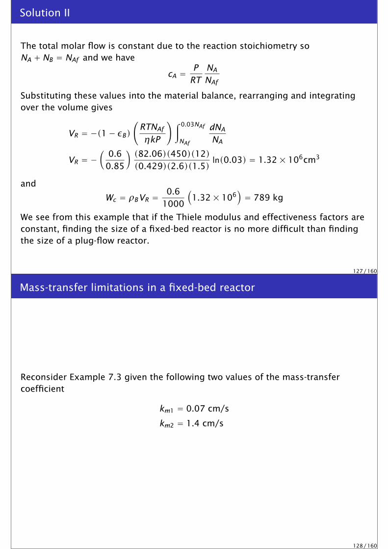
The total molar flow is constant due to the reaction stoichiometry soNA +NB = NAf and we have
cA = PRT
NA
NAf
Substituting these values into the material balance, rearranging and integratingover the volume gives
VR = −(1− εB)(
RTNAf
ηkP
)∫ 0.03NAf
NAf
dNA
NA
VR = −(
0.60.85
)(82.06)(450)(12)(0.429)(2.6)(1.5)
ln(0.03) = 1.32× 106cm3
and
Wc = ρBVR = 0.61000
(1.32× 10⁶
)= 789 kg
We see from this example that if the Thiele modulus and effectiveness factors areconstant, finding the size of a fixed-bed reactor is no more difficult than findingthe size of a plug-flow reactor.
127 / 160
Mass-transfer limitations in a fixed-bed reactor
Reconsider Example 7.3 given the following two values of the mass-transfercoefficient
km1 = 0.07 cm/s
km2 = 1.4 cm/s
128 / 160
Solution I
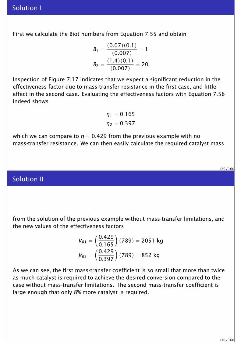
First we calculate the Biot numbers from Equation 7.55 and obtain
B1 = (0.07)(0.1)(0.007)
= 1
B2 = (1.4)(0.1)(0.007)= 20
Inspection of Figure 7.17 indicates that we expect a significant reduction in theeffectiveness factor due to mass-transfer resistance in the first case, and littleeffect in the second case. Evaluating the effectiveness factors with Equation 7.58indeed shows
η1 = 0.165
η2 = 0.397
which we can compare to η = 0.429 from the previous example with nomass-transfer resistance. We can then easily calculate the required catalyst mass
129 / 160
Solution II
from the solution of the previous example without mass-transfer limitations, andthe new values of the effectiveness factors
VR1 =(
0.4290.165
)(789) = 2051 kg
VR2 =(
0.4290.397
)(789) = 852 kg
As we can see, the first mass-transfer coefficient is so small that more than twiceas much catalyst is required to achieve the desired conversion compared to thecase without mass-transfer limitations. The second mass-transfer coefficient islarge enough that only 8% more catalyst is required.
130 / 160
Second-order, isothermal fixed-bed reactor
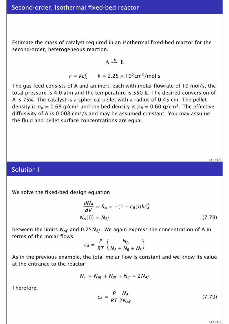
Estimate the mass of catalyst required in an isothermal fixed-bed reactor for thesecond-order, heterogeneous reaction.
Ak-→ B
r = kc2A k = 2.25× 105cm3/mol s
The gas feed consists of A and an inert, each with molar flowrate of 10 mol/s, thetotal pressure is 4.0 atm and the temperature is 550 K. The desired conversion ofA is 75%. The catalyst is a spherical pellet with a radius of 0.45 cm. The pelletdensity is ρp = 0.68 g/cm3 and the bed density is ρB = 0.60 g/cm3. The effectivediffusivity of A is 0.008 cm2/s and may be assumed constant. You may assumethe fluid and pellet surface concentrations are equal.
131 / 160
Solution I
We solve the fixed-bed design equation
dNA
dV= RA = −(1− εB)ηkc2
A
NA(0) = NAf (7.78)
between the limits NAf and 0.25NAf . We again express the concentration of A interms of the molar flows
cA = PRT
(NA
NA +NB +NI
)
As in the previous example, the total molar flow is constant and we know its valueat the entrance to the reactor
NT = NAf +NBf +NIf = 2NAf
Therefore,
cA = PRT
NA
2NAf(7.79)
132 / 160

Solution II
Next we use the definition of Φ for nth-order reactions given in Equation 7.42
Φ = R3
[(n + 1)kcn−1
A
2DA
]1/2
= R3
(n + 1)k
2DA
(P
RTNA
2NAf
)n−1
1/2
(7.80)
Substituting in the parameter values gives
Φ = 9.17
(NA
2NAf
)1/2
(7.81)
For the second-order reaction, Equation 7.81 shows that Φ varies with the molarflow, which means Φ and η vary along the length of the reactor as NA decreases.We are asked to estimate the catalyst mass needed to achieve a conversion of Aequal to 75%. So for this particular example, Φ decreases from 6.49 to 3.24. Asshown in Figure 7.9, we can approximate the effectiveness factor for thesecond-order reaction using the analytical result for the first-order reaction,Equation 7.38,
η = 1Φ
[1
tanh3Φ− 1
3Φ
](7.82)
133 / 160
Solution III
Summarizing so far, to compute NA versus VR, we solve one differential equation,Equation 7.78, in which we use Equation 7.79 for cA, and Equations 7.81 and 7.82for Φ and η. We march in VR until NA = 0.25NAf . The solution to the differentialequation is shown in Figure 7.26.
134 / 160

Solution IV
2
3
4
5
6
7
8
9
10
0 50 100 150 200 250 300 350 400
NA
(mo
l/s)
η = 1Φ
η = 1Φ
[1
tanh3Φ− 1
3Φ
]
VR (L)
135 / 160
Solution V
Figure 7.26: Molar flow of A versus reactor volume for second-order, isothermal reaction ina fixed-bed reactor.
The required reactor volume and mass of catalyst are:
VR = 361 L, Wc = ρBVR = 216 kg
As a final exercise, given that Φ ranges from 6.49 to 3.24, we can make the largeΦ approximation
η = 1Φ
(7.83)
to obtain a closed-form solution. If we substitute this approximation for η, andEquation 7.80 into Equation 7.78 and rearrange we obtain
dNA
dV= −(1− εB)
√k (P/RT )3/2
(R/3)√
3/DA(2NAf )3/2N3/2
A
136 / 160
Solution VI
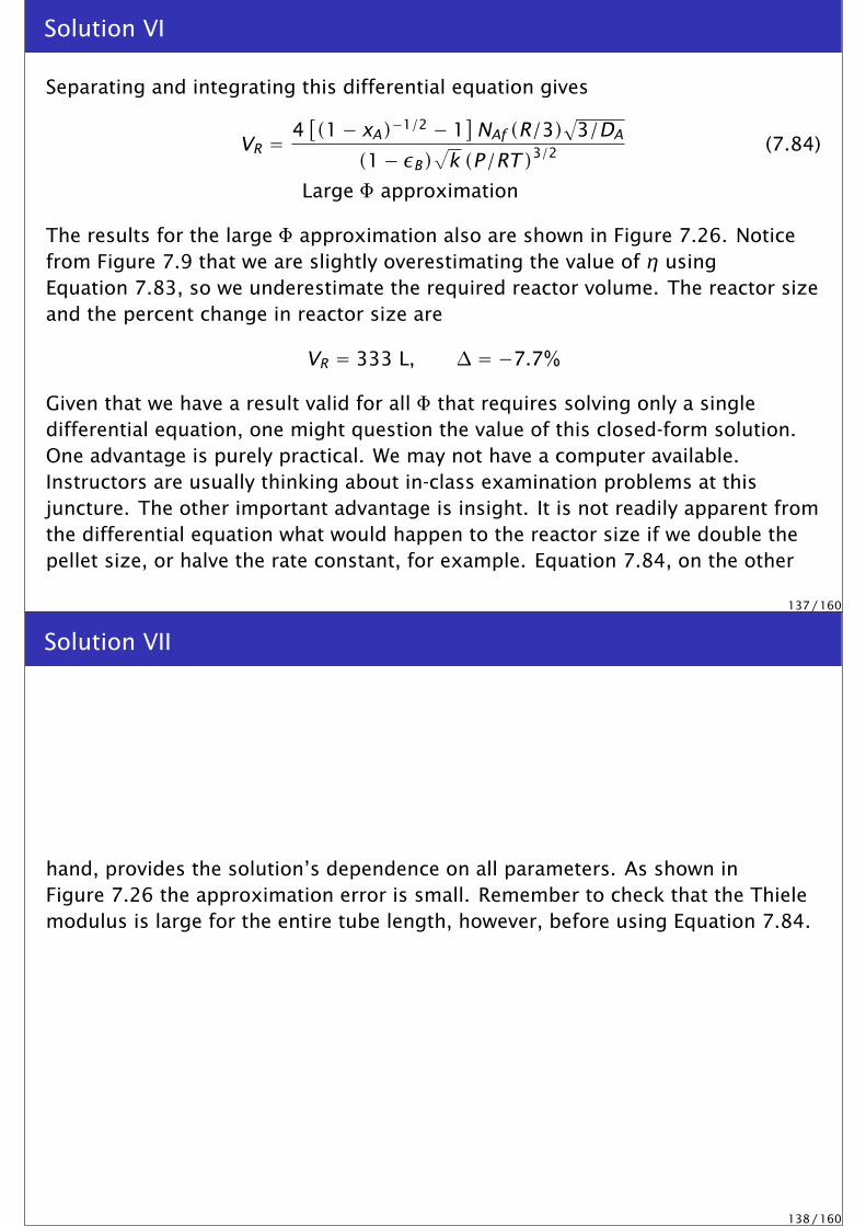
Separating and integrating this differential equation gives
VR = 4[(1− xA)−1/2 − 1
]NAf (R/3)
√3/DA
(1− εB)√
k (P/RT )3/2(7.84)
Large Φ approximation
The results for the large Φ approximation also are shown in Figure 7.26. Noticefrom Figure 7.9 that we are slightly overestimating the value of η usingEquation 7.83, so we underestimate the required reactor volume. The reactor sizeand the percent change in reactor size are
VR = 333 L, ∆ = −7.7%
Given that we have a result valid for all Φ that requires solving only a singledifferential equation, one might question the value of this closed-form solution.One advantage is purely practical. We may not have a computer available.Instructors are usually thinking about in-class examination problems at thisjuncture. The other important advantage is insight. It is not readily apparent fromthe differential equation what would happen to the reactor size if we double thepellet size, or halve the rate constant, for example. Equation 7.84, on the other
137 / 160
Solution VII
hand, provides the solution’s dependence on all parameters. As shown inFigure 7.26 the approximation error is small. Remember to check that the Thielemodulus is large for the entire tube length, however, before using Equation 7.84.
138 / 160

Hougen-Watson kinetics in a fixed-bed reactor
The following reaction converting CO to CO2 takes place in a catalytic, fixed-bedreactor operating isothermally at 838 K and 1.0 atm
CO+ 1/2O2 -→ CO2
The following rate expression and parameters are adapted from a different modelgiven by Oh et al. [8]. The rate expression is assumed to be of the Hougen-Watsonform
r = kcCOcO2
1+ KcCOmol/s cm3 pellet
The constants are provided below
k = 8.73× 10¹² exp(−13,500/T ) cm3/mol s
K = 8.099× 10⁶ exp(409/T ) cm3/mol
DCO = 0.0487 cm2/s
in which T is in Kelvin. The catalyst pellet radius is 0.1 cm. The feed to the reactorconsists of 2 mol% CO, 10 mol% O2, zero CO2 and the remainder inerts. Find thereactor volume required to achieve 95% conversion of the CO.
139 / 160
Solution
Given the reaction stoichiometry and the excess of O2, we can neglect the changein cO2 and approximate the reaction as pseudo-first order in CO
r = k′cCO
1+ KcCOmol/s cm3 pellet
k′ = kcO2f
which is of the form analyzed in Section 7.4.4. We can write the mass balance forthe molar flow of CO,
dNCO
dV= −(1− εB)ηr(cCO)
in which cCO is the fluid CO concentration. From the reaction stoichiometry, wecan express the remaining molar flows in terms of NCO
NO2 = NO2f + 1/2(NCO −NCOf )
NCO2 = NCOf −NCO
N = NO2f + 1/2(NCO +NCOf )
The concentrations follow from the molar flows assuming an ideal-gas mixture
cj = PRT
Nj
N
0.0× 100
2.0× 10⁻⁶
4.0× 10⁻⁶
6.0× 10⁻⁶
8.0× 10⁻⁶
1.0× 10⁻⁵
1.2× 10⁻⁵
1.4× 10⁻⁵
0 50 100 150 200 250
O2
CO2
CO
c j(m
ol/
cm3)
VR (cm3)
Figure 7.27: Molar concentrations versus reactor volume.
0
50
100
150
200
250
300
350
0 50 100 150 200 250
0
5
10
15
20
25
30
35
φ Φ
Φ φ
VR (cm3)
Figure 7.28: Dimensionless equilibrium constant and Thiele modulus versus reactorvolume. Values indicate η = 1/Φ is a good approximation for entire reactor.
To decide how to approximate the effectiveness factor shown in Figure 7.14, weevaluate φ = KC0cC0, at the entrance and exit of the fixed-bed reactor. With φevaluated, we compute the Thiele modulus given in Equation 7.52 and obtain
φ = 32.0 Φ= 79.8, entrance
φ = 1.74 Φ = 326, exit
It is clear from these values and Figure 7.14 that η = 1/Φ is an excellentapproximation for this reactor. Substituting this equation for η into the massbalance and solving the differential equation produces the results shown inFigure 7.27. The concentration of O2 is nearly constant, which justifies thepseudo-first-order rate expression. Reactor volume
VR = 233 L
is required to achieve 95% conversion of the CO. Recall that the volumetricflowrate varies in this reactor so conversion is based on molar flow, not molarconcentration. Figure 7.28 shows how Φ and φ vary with position in the reactor.In the previous examples, we have exploited the idea of an effectiveness factor toreduce fixed-bed reactor models to the same form as plug-flow reactor models.This approach is useful and solves several important cases, but this approach isalso limited and can take us only so far. In the general case, we must contend withmultiple reactions that are not first order, nonconstant thermochemicalproperties, and nonisothermal behavior in the pellet and the fluid. For thesecases, we have no alternative but to solve numerically for the temperature andspecies concentrations profiles in both the pellet and the bed. As a final example,we compute the numerical solution to a problem of this type.We use the collocation method to solve the next example, which involves fivespecies, two reactions with Hougen-Watson kinetics, both diffusion and externalmass-transfer limitations, and nonconstant fluid temperature, pressure andvolumetric flowrate.
140 / 160

Multiple-reaction, nonisothermal fixed-bed reactor
Evaluate the performance of the catalytic converter in converting CO andpropylene.Determine the amount of catalyst required to convert 99.6% of the CO andpropylene.The reaction chemistry and pellet mass-transfer parameters are given in Table 7.5.The feed conditions and heat-transfer parameters are given in Table 7.6.
141 / 160
Feed conditions and heat-transfer parameters
Parameter Value UnitsPf 2.02× 10⁵ N/m2
Tf 550 KRt 5.0 cmuf 75 cm/sTa 325 KUo 5.5× 10⁻³ cal/(cm2 Ks)∆HR1 −67.63× 10³ cal/(mol CO K)∆HR2 −460.4× 10³ cal/(mol C3H6 K)
Cp 0.25 cal/(g K)µf 0.028× 10⁻² g/(cm s)ρb 0.51 g/cm3
ρp 0.68 g/cm3
Table 7.6: Feed flowrate and heat-transfer parameters for the fixed-bed catalytic converter.
142 / 160

Solution
The fluid balances govern the change in the fluid concentrations, temperatureand pressure.
The pellet concentration profiles are solved with the collocation approach.
The pellet and fluid concentrations are coupled through the mass-transferboundary condition.
The fluid concentrations are shown in Figure 7.29.
A bed volume of 1098 cm3 is required to convert the CO and C3H6.Figure 7.29 also shows that oxygen is in slight excess.
143 / 160
10−11
10−10
10−9
10−8
10−7
10−6
10−5
0 200 400 600 800 1000 1200
cO2
cCO
cC3H6
c j(m
ol/
cm3)
VR (cm3)
Figure 7.29: Fluid molar concentrations versus reactor volume.
144 / 160

Solution I
The reactor temperature and pressure are shown in Figure 7.30.The feed enters at 550 K, and the reactor experiences about a 130 Ktemperature rise while the reaction essentially completes; the heat lossesthen reduce the temperature to less than 500 K by the exit.
The pressure drops from the feed value of 2.0 atm to 1.55 atm at the exit.Notice the catalytic converter exit pressure of 1.55 atm must be large enoughto account for the remaining pressure drops in the tail pipe and muffler.
145 / 160
Solution II
480
500
520
540
560
580
600
620
640
660
680
0 200 400 600 800 1000 12001.55
1.6
1.65
1.7
1.75
1.8
1.85
1.9
1.95
2
T(K
)
P(a
tm)T
P
VR (cm3)
Figure 7.30: Fluid temperature and pressure versus reactor volume.
146 / 160

Solution
In Figures 7.31 and 7.32, the pellet CO concentration profile at several reactorpositions is displayed.
We see that as the reactor heats up, the reaction rates become large and theCO is rapidly converted inside the pellet.
By 490 cm3 in the reactor, the pellet exterior CO concentration has droppedby two orders of magnitude, and the profile inside the pellet has become verysteep.
As the reactions go to completion and the heat losses cool the reactor, thereaction rates drop. At 890 cm3, the CO begins to diffuse back into the pellet.
Finally, the profiles become much flatter near the exit of the reactor.
147 / 160
490900 890 990 1098
VR (cm3)
40
Ã Ä Å ÆÂÁÀ
Figure 7.31: Reactor positions for pellet profiles.
148 / 160

10−15
10−14
10−13
10−12
10−11
10−10
10−9
10−8
10−7
10−6
0 0.05 0.1 0.15 0.175
À Á Â
ÃÄ
Å
Æ
c CO
(mo
l/cm
3)
r (cm)
Figure 7.32: Pellet CO profiles at several reactor positions.
149 / 160
It can be numerically challenging to calculate rapid changes and steep profilesinside the pellet.
The good news, however, is that accurate pellet profiles are generally notrequired for an accurate calculation of the overall pellet reaction rate. Thereason is that when steep profiles are present, essentially all of the reactionoccurs in a thin shell near the pellet exterior.
We can calculate accurately down to concentrations on the order of 10−15 asshown in Figure 7.32, and by that point, essentially zero reaction is occurring,and we can calculate an accurate overall pellet reaction rate.
It is always a good idea to vary the numerical approximation in the pelletprofile, by changing the number of collocation points, to ensure convergencein the fluid profiles.
Congratulations, we have finished the most difficult example in the text.
150 / 160

Summary
This chapter treated the fixed-bed reactor, a tubular reactor packed withcatalyst pellets.
We started with a general overview of the transport and reaction events thattake place in the fixed-bed reactor: transport by convection in the fluid;diffusion inside the catalyst pores; and adsorption, reaction and desorptionon the catalyst surface.
In order to simplify the model, we assumed an effective diffusivity could beused to describe diffusion in the catalyst particles.
We next presented the general mass and energy balances for the catalystparticle.
151 / 160
Summary
Next we solved a series of reaction-diffusion problems in a single catalystparticle. These included:
Single reaction in an isothermal pellet. This case was further divided into anumber of special cases.
First-order, irreversible reaction in a spherical particle.Reaction in a semi-infinite slab and cylindrical particle.nth order, irreversible reaction.Hougen-Watson rate expressions.Particle with significant external mass-transfer resistance.
Single reaction in a nonisothermal pellet.Multiple reactions.
152 / 160
Summary
For the single-reaction cases, we found a dimensionless number, the Thielemodulus (Φ), which measures the rate of production divided by the rate ofdiffusion of some component.
We summarized the production rate using the effectiveness factor (η), theratio of actual rate to rate evaluated at the pellet exterior surface conditions.
For the single-reaction, nonisothermal problem, we solved the so-calledWeisz-Hicks problem, and determined the temperature and concentrationprofiles within the pellet. We showed the effectiveness factor can be greaterthan unity for this case. Multiple steady-state solutions also are possible forthis problem.
For complex reactions involving many species, we must solve numerically thecomplete reaction-diffusion problem. These problems are challengingbecause of the steep pellet profiles that are possible.
153 / 160
Summary
Finally, we showed several ways to couple the mass and energy balances overthe fluid flowing through a fixed-bed reactor to the balances within the pellet.
For simple reaction mechanisms, we were still able to use the effectivenessfactor approach to solve the fixed-bed reactor problem.
For complex mechanisms, we solved numerically the full problem given inEquations 7.67–7.77.
We solved the reaction-diffusion problem in the pellet coupled to the massand energy balances for the fluid, and we used the Ergun equation tocalculate the pressure in the fluid.
154 / 160
Notation I
a characteristic pellet length, Vp/Sp
Ac reactor cross-sectional areaB Biot number for external mass transferc constant for the BET isothermcj concentration of species jcjs concentration of species j at the catalyst surfacec dimensionless pellet concentrationcm total number of active surface sitesDAB binary diffusion coefficientDj effective diffusion coefficient for species jDjK Knudsen diffusion coefficient for species jDjm diffusion coefficient for species j in the mixtureDp pellet diameterEdiff activation energy for diffusionEobs experimental activation energyErxn intrinsic activation energy for the reaction∆HRi heat of reaction iIj rate of transport of species j into a pelletI0 modified Bessel function of the first kind, zero orderI1 modified Bessel function of the first kind, first order
155 / 160
Notation II
ke effective thermal conductivity of the pelletkmj mass-transfer coefficient for species jkn nth-order reaction rate constantL pore lengthMj molecular weight of species jnr number of reactions in the reaction networkN total molar flow,
∑j Nj
Nj molar flow of species jP pressureQ volumetric flowrater radial coordinate in catalyst particlera average pore radiusri rate of reaction i per unit reactor volumerobs observed (or experimental) rate of reaction in the pelletrip total rate of reaction i per unit catalyst volumer dimensionless radial coordinateR spherical pellet radiusR gas constantRj production rate of species jRjf production rate of species j at bulk fluid conditions
156 / 160
Notation III
Rjp total production rate of species j per unit catalyst volumeRjs production rate of species j at the pellet surface conditionsSg BET area per gram of catalystSp external surface area of the catalyst pelletT temperatureTf bulk fluid temperatureTs pellet surface temperatureUo overall heat-transfer coefficientv volume of gas adsorbed in the BET isothermvm volume of gas corresponding to an adsorbed monolayerV reactor volume coordinateVg pellet void volume per gram of catalystVp volume of the catalyst pelletVR reactor volumeWc total mass of catalyst in the reactoryj mole fraction of species jz position coordinate in a slabε porosity of the catalyst pelletεB fixed-bed porosity or void fractionη effectiveness factor
157 / 160
Notation IV
λ mean free pathµf bulk fluid densityνij stoichiometric number for the jth species in the ith reactionξ integral of a diffusing species over a bounding surfaceρ bulk fluid densityρB reactor bed densityρp overall catalyst pellet densityρs catalyst solid-phase densityσ hard sphere collision radiusτ tortuosity factorΦ Thiele modulusΩD,AB dimensionless function of temperature and the intermolecular potential field for
one molecule of A and one molecule of B
158 / 160

References I
R. Aris.
A normalization for the Thiele modulus.Ind. Eng. Chem. Fundam., 4:227, 1965.
R. Aris.
The Mathematical Theory of Diffusion and Reaction in Permeable Catalysts. Volume I: The Theory of theSteady State.Clarendon Press, Oxford, 1975.
R. B. Bird, W. E. Stewart, and E. N. Lightfoot.
Notes on Transport Phenomena.John Wiley & Sons, New York, 1958.
K. B. Bischoff.
Effectiveness factors for general reaction rate forms.AIChE J., 11:351, 1965.
S. Brunauer, P. H. Emmett, and E. Teller.
Adsorption of gases in multimolecular layers.J. Am. Chem. Soc., 60:309–319, 1938.
S. Ergun.
Fluid flow through packed columns.Chem. Eng. Prog., 48(2):89–94, 1952.
B. C. Gates.
Catalytic Chemistry.John Wiley & Sons, New York, 1992.
159 / 160
References II
S. H. Oh, J. C. Cavendish, and L. L. Hegedus.
Mathematical modeling of catalytic converter lightoff: Single-pellet studies.AIChE J., 26(6):935–943, 1980.
C. J. Pereira, J. B. Wang, and A. Varma.
A justification of the internal isothermal model for gas-solid catalytic reactions.AIChE J., 25(6):1036–1043, 1979.
E. E. Petersen.
A general criterion for diffusion influenced chemical reactions in porous solids.Chem. Eng. Sci., 20:587–591, 1965.
E. W. Thiele.
Relation between catalytic activity and size of particle.Ind. Eng. Chem., 31(7):916–920, 1939.
P. B. Weisz.
Zeolites - new horizons in catalysts.Chem. Tech., 3:498, 1973.
P. B. Weisz and J. S. Hicks.
The behaviour of porous catalyst particles in view of internal mass and heat diffusion effects.Chem. Eng. Sci., 17:265–275, 1962.
160 / 160