Embed Size (px)
Citation preview
Econometrica, Vol. 76, No. 1 (January, 2008), 155-174
NOTES AND COMMENTS
HETEROSKEDASTICITY-ROBUST STANDARD ERRORS FOR FIXED EFFECTS PANEL DATA REGRESSION
BY JAMES H. STOCK AND MARK W. WATSON1
The conventional heteroskedasticity-robust (HR) variance matrix estimator for cross-sectional regression (with or without a degrees-of-freedom adjustment), applied to the fixed-effects estimator for panel data with serially uncorrelated errors, is incon- sistent if the number of time periods T is fixed (and greater than 2) as the number of entities n increases. We provide a bias-adjusted HR estimator that is NVn-T-consistent under any sequences (n, T) in which n and/or T increase to cc. This estimator can be extended to handle serial correlation of fixed order.
KEYWORDS: White standard errors, longitudinal data, clustered standard errors.
1. MODEL AND THEORETICAL RESULTS
CONSIDER THE FIXED-EFFECTS REGRESSION MODEL
(1) Yit = ai + •tXit
+ uit, i = 1, . . . , n, t = 1, . . . , T,
where Xit is a k x 1 vector of strictly exogenous regressors and the error, uit, is conditionally serially uncorrelated but possibly heteroskedastic. Let the tilde (-) over variables denote deviations from entity means (Xit = Xit -
T-1 CsT_ Xji, etc.). Suppose that (Xi,, ui,) satisfies the following assumptions:
ASSUMPTION 1: (Xil, . , Xi, uil, , . . . , uiT) are independent and identically distributed (i.i.d.) over i = 1, ..., n (i.i.d. over entities).
ASSUMPTION 2: E(uit Xil, ..., XiT) = 0 (strict exogeneity).
ASSUMPTION 3: Qek - ET-' ET=, XitXi, is nonsingular (no perfect multi-
collinearity).
ASSUMPTION 4: E(uitUisIXil, .. . , Xir) = Ofor t =A s (conditionally serially un- correlated errors).
For the asymptotic results we make a further assumption:
ASSUMPTION 5 -Stationarity and Moment Condition: (Xit, uit) is stationary and has absolutely summable cumulants up to order 12.
'We thank Alberto Abadie, Gary Chamberlain, Guido Imbens, Doug Staiger, Hal White, and the referees for helpful comments and/or discussions, Mitchell Peterson for providing the data in footnote 2, and Anna Mikusheva for research assistance. This research was supported in part by NSF Grant SBR-0617811.
155

156 J. H. STOCK AND M. W WATSON
The fixed-effects estimator is
A n T -1
(2) PFE = (Cfi ; X• L~ X~f' i=1 t=l i=1 t=l
The asymptotic distribution of pFE is (e.g., Arrelano (2003))
d- -1 (3) /-T(f3FE - p) -d N(0, Q
S•ZQ- '),
where -=7 E(Xitu)
t=1
The variance of the asymptotic distribution in (3) is estimated by Q~ -QjJ , where Qg = (nT)- i= z t=1,XitX
and 2 is a heteroskedasticity-robust (HR) covariance matrix estimator.
A frequently used HR estimator of , is
n T 1 - ^2
(4) HR-XS
=XitXituit nT -n-k
i=1 t=1
where { uit are the fixed-effects regression residuals, uit = iit - (/FE - 3)'Xit.2 Although VHR-XS is consistent in cross-section regression (White (1980)), it
turns out to be inconsistent in panel data regression with fixed T. Specifically, an implication of the results in the Appendix is that, under fixed-T asymptotics with T > 2,
P 1 (5) .HR-XS (B-),
(n---oo,T fixed) T - 1
where B=E E X it T [( T T
t= 1s=l J
The expression for B in (5) suggests the bias-adjusted estimator
(6) wHR-FE __
(HR-XS - B
T-2 T-1
2For example, at the time of writing, VHR-XS is the HR panel data variance estimator used in STATA and Eviews. Petersen (2007) reported a survey of 207 panel data papers published in the Journal of Finance, the Journal of Financial Economics, and the Review of Financial Studies between 2001 and 2004. Of these, 15% used XHR-XS, 23% used clustered standard errors, 26% used uncorrected ordinary least squares standard errors, and the remaining papers used other methods.
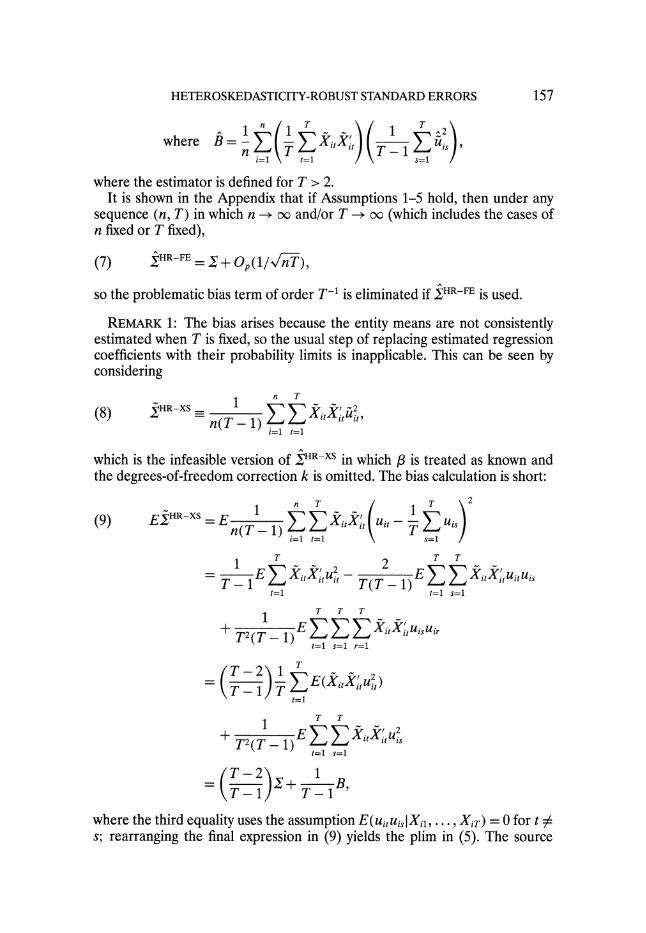
HETEROSKEDASTICITY-ROBUST STANDARD ERRORS 157
AA1 1 - 1 -~2 where B=- XitXj T - 1 uis , Si=1 Zt=
1 s=l
where the estimator is defined for T > 2. It is shown in the Appendix that if Assumptions 1-5 hold, then under any
sequence (n, T) in which n -+ oc and/or T - oo (which includes the cases of n fixed or T fixed),
(7) +HR-FE = + Op(1/ n-T),
so the problematic bias term of order T-1 is eliminated if XHR-FE is used.
REMARK 1: The bias arises because the entity means are not consistently estimated when T is fixed, so the usual step of replacing estimated regression coefficients with their probability limits is inapplicable. This can be seen by considering
n T
(8) HR-XS Xn(T1)Xiuit i=1
t=l
which is the infeasible version of ?HR-XS in which P is treated as known and the degrees-of-freedom correction k is omitted. The bias calculation is short:
1 RX11 (9) EHR-XS =
En(T-1) X (t Uit - T is
1 T2 T(T
__ XitXit
ittgis T - 1E XX
uit T(T - 1) t=1 t=l s=1
+ T2T-XitXitUisuir t=1 s=1 r=1
(TT-2)1 T 1 )T E(XitXitu) t=l
+ T2 (TI) 1)E XiXi-tU t=1 s=1
(T-2 + B
where the third equality uses the assumption E(uituis
Xil,..., Xir) = 0 for t / s; rearranging the final expression in (9) yields the plim in (5). The source
158 J. H. STOCK AND M. W WATSON
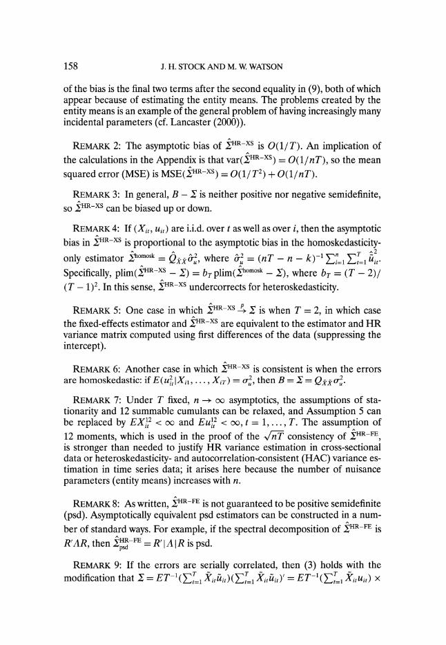
of the bias is the final two terms after the second equality in (9), both of which appear because of estimating the entity means. The problems created by the entity means is an example of the general problem of having increasingly many incidental parameters (cf. Lancaster (2000)).
REMARK 2: The asymptotic bias of 2HR-XS is 0(1/ T). An implication of the calculations in the Appendix is that var(~HR-XS) = O(1/nT), so the mean
squared error (MSE) is MSE(HR-XS) = 0(1/T2) + O(1/nT).
REMARK 3: In general, B - V is neither positive nor negative semidefinite, so SHR-XS can be biased up or down.
REMARK 4: If (Xit, Uit) are i.i.d. over t as well as over i, then the asymptotic bias in XHR-XS is proportional to the asymptotic bias in the homoskedasticity-
only estimator homosk = Q , where ur = (nT - n - k)-1 7=E,= T= Uit.
Specifically, plim(CHR-XS - I) = bT plim(Ihomosk - 1), where bT = (T - 2)/ (T - 1)2. In this sense, XHR-XS undercorrects for heteroskedasticity.
REMARK 5: One case in which VHR-XSP - is when T = 2, in which case the fixed-effects estimator and YHR-XS are equivalent to the estimator and HR variance matrix computed using first differences of the data (suppressing the intercept).
REMARK 6: Another case in which XHR-XS is consistent is when the errors are homoskedastic: if E(uIX,1, ... , XiT) = u2, then B = =
Q2o-,2u. REMARK 7: Under T fixed, n -- 00 asymptotics, the assumptions of sta-
tionarity and 12 summable cumulants can be relaxed, and Assumption 5 can be replaced by EX 12 < 00 and EU12 < 0o, t = 1, ..., T. The assumption of 12 moments, which is used in the proof of the , T consistency of HR-FE, is stronger than needed to justify HR variance estimation in cross-sectional data or heteroskedasticity- and autocorrelation-consistent (HAC) variance es- timation in time series data; it arises here because the number of nuisance parameters (entity means) increases with n.
REMARK 8: As written, iHR-FE is not guaranteed to be positive semidefinite (psd). Asymptotically equivalent psd estimators can be constructed in a num- ber of standard ways. For example, if the spectral decomposition of iHR-FE is
R'AR, then -HR-FE
= R' IARispsd
REMARK 9: If the errors are serially correlated, then (3) holds with the modification that Z =
ET-l(•r= Xitu)(UEtr Xii)' = ET-1(=>,=1 Xtut) x
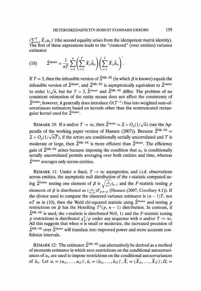
HETEROSKEDASTICITY-ROBUST STANDARD ERRORS 159
(ZT=1 SXiui,)'
(the second equality arises from the idempotent matrix identity). The first of these expressions leads to the "clustered" (over entities) variance estimator
(10)
•cYluster_= 1 i•itit Xis Uis
i=n 1 t=l s=l1
If T = 3, then the infeasible version of XHR-FE (in which P is known) equals the infeasible version of Xcluster, and XHR-FE is asymptotically equivalent to Xcluster
to order 11/1-n, but for T > 3, Xcluster and XHR-FE differ. The problem of no consistent estimation of the entity means does not affect the consistency of
Xcluster; however, it generally does introduce O(T-1) bias into weighted sum-of- covariances estimators based on kernels other than the nontruncated rectan- gular kernel used for
Xcluster.
REMARK 10: If n and/or T -+ 00, then Icluster = •
+ Op(1/-n)
(see the Ap-
pendix of the working paper version of Hansen (2007)). Because XHR-FE =
+ + O,(1/vfT), if the errors are conditionally serially uncorrelated and T is moderate or large, then sHR-FE is more efficient than Xcluster. The efficiency gain of .HR-FE arises because imposing the condition that
uit is conditionally
serially uncorrelated permits averaging over both entities and time, whereas Xcluster averages only across entities.
REMARK 11: Under n fixed, T -+ o0 asymptotics, and i.i.d. observations across entities, the asymptotic null distribution of the t-statistic computed us-
ing Icluster testing one element of 3 is tn-1
and the F-statistic testing p elements of p is distributed as (~n )Fp,n-p (Hansen (2007, Corollary 4.1)). If the divisor used to compute the clustered variance estimator is (n - 1) T, not nT as in (10), then the Wald chi-squared statistic using Xcluster and testing p restrictions on / has the Hotelling T2(p, n - 1) distribution. In contrast, if XHR-FE is used, the t-statistic is distributed N(0, 1) and the F-statistic testing p restrictions is distributed X,/lp under any sequence with n and/or T -- 00.
All this suggests that when n is small or moderate, the increased precision of 1HR-FE over .cluster will translate into improved power and more accurate con- fidence intervals.
REMARK 12: The estimator IHR-FE can alternatively be derived as a method of moments estimator in which zero restrictions on the conditional autocovari- ances of ui, are used to impose restrictions on the conditional autocovariances
of u;it"
Let ui =
(Uil, ..., Uir)', li
=
(/i/1, ".., /ir)',
Xi = (Xil,
... Xir)', "i
=
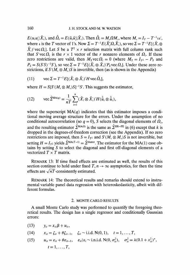
160 J. H. STOCK AND M. W WATSON
E(uiuj'Xi), and Qi =
E(&iiXiiiXi). Then Q i = MjQM,, where M, = IT - T-l ',
where t is the T vector of l's. Now I = T-1E(XjfljXi), so vec = = T-'E[(X) i Xi)'vecQl]. Let S be a T2 X r selection matrix with full column rank such that S'vec?2i is the r x 1 vector of the r nonzero elements of Q,. If these zero restrictions are valid, then Ms vec ni = 0 (where Ms = IT2 - Ps and Ps = S(S'S)-1S'), so vec
- = T-'E[(Xi 0 X)'Ps
veci/]. Under these zero re-
strictions, if S'(M, 0 M,)S is invertible, then (as is shown in the Appendix)
(11) vec = T-'E[(Xi 0 Xi)'H vec hi],
where H = S[S'(M, 0 M,)S]-'S'. This suggests the estimator,
(12) vec IMA(q) = (X, 0 Xi)'H(ui
0 ui),
i=1
where the superscript MA(q) indicates that this estimator imposes a condi- tional moving average structure for the errors. Under the assumption of no conditional autocorrelation (so q = 0), S selects the diagonal elements of Qi, and the resulting estimator 'MA(0) is the same as XHR-FE in (6) except that k is dropped in the degrees-of-freedom correction (see the Appendix). If no zero restrictions are imposed, then S = IT2 and S'(M, 0 M,)S is not invertible, but
setting H = IT2 yields =MA(T-1) ._ cluster. The estimator for the MA(1) case ob- tains by setting S to select the diagonal and first off-diagonal elements of a vectorized T x T matrix.
REMARK 13: If time fixed effects are estimated as well, the results of this section continue to hold under fixed T, n -+ *o asymptotics, for then the time effects are 1/HT-consistently estimated.
REMARK 14: The theoretical results and remarks should extend to instru- mental variable panel data regression with heteroskedasticity, albeit with dif- ferent formulas.
2. MONTE CARLO RESULTS
A small Monte Carlo study was performed to quantify the foregoing theo- retical results. The design has a single regressor and conditionally Gaussian errors:
(13) Yit = xit + Uit,
(14) xit = itj- +Oi1, it
~ i.i.d. N(0, 1) ,=, t = 1,..., T,
(15) Uit =
;it + Osit-1, fit[Xi x; i.n.i.d. N(0, 0,-), o-2
= A(0.1 + xt)K,
t=l,..., T,
HETEROSKEDASTICITY-ROBUST STANDARD ERRORS 161
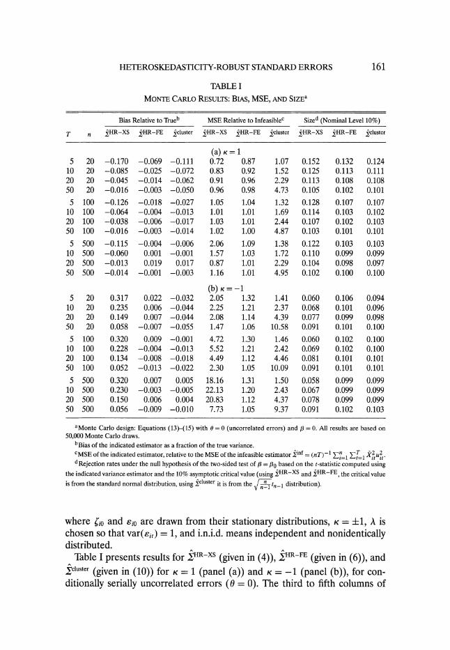
TABLE I MONTE CARLO RESULTS: BIAS, MSE, AND SIZEa
Bias Relative to Trueb MSE Relative to Infeasiblec Sized (Nominal Level 10%)
T n ?HR-XS ?HR-FE cluster HR-XS ?HR-FE cluster XHR-XS ?HR-FE cluster
(a) K = 1 5 20 -0.170 -0.069 -0.111 0.72 0.87 1.07 0.152 0.132 0.124
10 20 -0.085 -0.025 -0.072 0.83 0.92 1.52 0.125 0.113 0.111 20 20 -0.045 -0.014 -0.062 0.91 0.96 2.29 0.113 0.108 0.108 50 20 -0.016 -0.003 -0.050 0.96 0.98 4.73 0.105 0.102 0.101
5 100 -0.126 -0.018 -0.027 1.05 1.04 1.32 0.128 0.107 0.107 10 100 -0.064 -0.004 -0.013 1.01 1.01 1.69 0.114 0.103 0.102 20 100 -0.038 -0.006 -0.017 1.03 1.01 2.44 0.107 0.102 0.103 50 100 -0.016 -0.003 -0.014 1.02 1.00 4.87 0.103 0.101 0.101
5 500 -0.115 -0.004 -0.006 2.06 1.09 1.38 0.122 0.103 0.103 10 500 -0.060 0.001 -0.001 1.57 1.03 1.72 0.110 0.099 0.099 20 500 -0.013 0.019 0.017 0.87 1.01 2.29 0.104 0.098 0.097 50 500 -0.014 -0.001 -0.003 1.16 1.01 4.95 0.102 0.100 0.100
(b) K= --1 5 20 0.317 0.022 -0.032 2.05 1.32 1.41 0.060 0.106 0.094
10 20 0.235 0.006 -0.044 2.25 1.21 2.37 0.068 0.101 0.096 20 20 0.149 0.007 -0.044 2.08 1.14 4.39 0.077 0.099 0.098 50 20 0.058 -0.007 -0.055 1.47 1.06 10.58 0.091 0.101 0.100
5 100 0.320 0.009 -0.001 4.72 1.30 1.46 0.060 0.102 0.100 10 100 0.228 -0.004 -0.013 5.52 1.21 2.42 0.069 0.102 0.100 20 100 0.134 -0.008 -0.018 4.49 1.12 4.46 0.081 0.101 0.101 50 100 0.052 -0.013 -0.022 2.30 1.05 10.09 0.091 0.101 0.101
5 500 0.320 0.007 0.005 18.16 1.31 1.50 0.058 0.099 0.099 10 500 0.230 -0.003 -0.005 22.13 1.20 2.43 0.067 0.099 0.099 20 500 0.150 0.006 0.004 20.83 1.12 4.37 0.078 0.099 0.099 50 500 0.056 -0.009 -0.010 7.73 1.05 9.37 0.091 0.102 0.103
aMonte Carlo design: Equations (13)-(15) with 0 = 0 (uncorrelated errors) and / = 0. All results are based on 50,000 Monte Carlo draws.
bBias of the indicated estimator as a fraction of the true variance. cMSE of the indicated estimator, relative to the MSE of the infeasible estimator finf =(nT)-l
•i1 T=2- uj2 --t= it
it" dRejection rates under the null hypothesis of the two-sided test of P = Pg based on the t-statistic computed using the indicated variance estimator and the 10% asymptotic critical value (using XHR-XS and XHR-FE, the critical value
is from the standard normal distribution, using Xcluster it is from the ? tn-1 distribution).
where ?io and eio are drawn from their stationary distributions, K = +1, A is chosen so that var(Eit) = 1, and i.n.i.d. means independent and nonidentically distributed.
Table I presents results for iHR-XS (given in (4)), JHR-FE (given in (6)), and Icluster (given in (10)) for K = 1 (panel (a)) and K = -1 (panel (b)), for con- ditionally serially uncorrelated errors (0 = 0). The third to fifth columns of
162 J. H. STOCK AND M. W. WATSON
Table I report the bias of the three estimators, relative to the true value of X
(e.g., E(XHR-XS - )/I). The next three columns report their MSEs relative to the MSE of the infeasible HR estimator in'f = (nT)-1 in
%
zT=I XitX;tu, that could be computed were the entity means and 3 known. The final three columns report the size of the 10% two-sided tests of P = 3o based on the t-statistic using the indicated variance estimator and asymptotic critical value
(standard normal for HR-XS and XHR-FE n-
t- for cluster). Several results
are noteworthy. First, the bias in XHR-XS can be large, it persists as n increases with T fixed,
and it can be positive or negative depending on the design. For example, with T = 5 and n = 500, the relative bias of XHR-XS is -11.5% when K = 1 and is 32% when K = -1. This large bias of VHR-XS can produce a very large relative MSE. Interestingly, in some cases with small n and T, and K = 1, the MSE of
,HR-XS is less than the MSE of the infeasible estimator, apparently reflecting a
bias-variance trade-off. Second, the bias correction in XHR-FE does its job: the relative bias of XHR-FE
is less than 2% in all cases with n > 100, and in most cases the MSE of XHR-FE
is very close to the MSE of the infeasible HR estimator. Third, consistent with Remark 12, the ratio of the MSE of the cluster vari-
ance estimator to the infeasible estimator depends on T and does not converge to 1 as n gets large for fixed T. The MSE of Xcluster considerably exceeds the MSE of XHR-FE when T is moderate or large, regardless of n.
Fourth, although the focus of this note has been bias and MSE, in practice variance estimators are used mainly for inference on 3, and one would suspect that the variance estimators with less bias would produce tests of P = go with
better size. Table I is consistent with this conjecture: when IHR-XS is biased
up, the t-tests reject too infrequently, and when XHR-XS is biased down, the t- tests reject too often. When T is small, the magnitudes of these size distortions can be considerable: for T = 5 and n = 500, the size of the nominal 10% test is 12.2% for K = 1 and is 5.8% when K = -1. In contrast, in all cases with n = 500, tests based on CHR-FE and clCuster have sizes within Monte Carlo error of 10%. In unreported designs with greater heteroskedasticity, the size distortions of tests based on XHR-xs are even larger than reported in Table I.
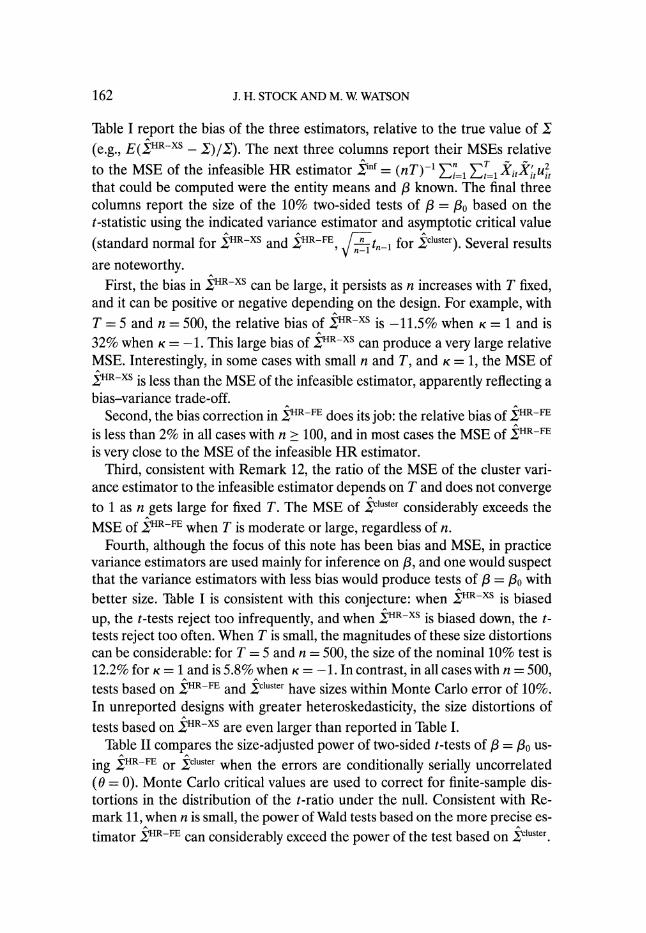
Table II compares the size-adjusted power of two-sided t-tests of /3 = /3o us-
ing 1HR-FE Or 1cluster when the errors are conditionally serially uncorrelated (6 = 0). Monte Carlo critical values are used to correct for finite-sample dis- tortions in the distribution of the t-ratio under the null. Consistent with Re- mark 11, when n is small, the power of Wald tests based on the more precise es- timator ?HR-FE can considerably exceed the power of the test based on
?cluster
HETEROSKEDASTICITY-ROBUST STANDARD ERRORS 163
TABLE II
SIZE-ADJUSTED POWER OF LEVEL-10% Two-SIDED WALD TESTS OF P = 0 AGAINST THE LOCAL ALTERNATIVE 3= b/V,/
a
Size-Adjusted Power of z-Test Based on:
n XjHR-FE cluster
(a) b =2 3 0.338 0.227 5 0.324 0.269
10 0.332 0.305 20 0.322 0.307
100 0.321 0.316
(b) b =4 3 0.758 0.504 5 0.750 0.629
10 0.760 0.710 20 0.760 0.731
100 0.761 0.756
aMonte Carlo design: Equations (13)-(15) with p = 0, K = 1, 0 = 0 (uncorrelated errors), and T = 20. Entries are Monte Carlo rejection rates of two-sided t-tests using the indicated variance estimator, with a critical value computed by Monte Carlo. Results are based on 50,000 Monte Carlo draws.
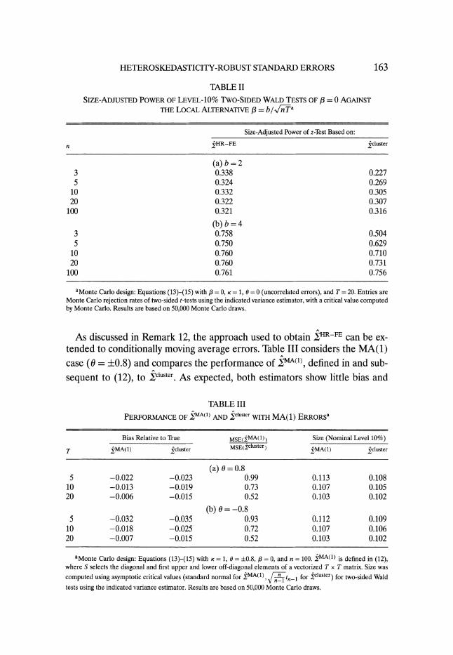
As discussed in Remark 12, the approach used to obtain ZHRFE can be ex- tended to conditionally moving average errors. Table III considers the MA(1) case (0 = ?0.8) and compares the performance of vMA1), defined in and sub-
sequent to (12), to Xcluster. As expected, both estimators show little bias and
TABLE III
PERFORMANCE OF MA(1) AND cluster WITH MA(1) ERRORSa
Bias Relative to True MSE(XMA(1)) Size (Nominal Level 10%)
T •MA(1)
?cluster MSE(cluster)
,MA(1)
cluster
(a) 6 = 0.8 5 -0.022 -0.023 0.99 0.113 0.108
10 -0.013 -0.019 0.73 0.107 0.105 20 -0.006 -0.015 0.52 0.103 0.102
(b) 0= -0.8 5 -0.032 -0.035 0.93 0.112 0.109
10 -0.018 -0.025 0.72 0.107 0.106 20 -0.007 -0.015 0.52 0.103 0.102
aMonte Carlo design: Equations (13)-(15) with K = 1, O = ?0.8,/3 = 0, and n = 100. ?^MA(1) is defined in (12), where S selects the diagonal and first upper and lower off-diagonal elements of a vectorized T x T matrix. Size was
computed using asymptotic critical values (standard normal for ,MA(1), _tn-1
for dcluster) for two-sided Wald tests using the indicated variance estimator. Results are based on 50,000 Monte Carlo draws.
164 J. H. STOCK AND M. W. WATSON
produce Wald tests with small or negligible size distortions. Because IMA(1)
in effect estimates fewer covariances than ?custer, however, XMA(1) has a lower MSE than Icluster, with its relative precision increasing as T increases.
3. CONCLUSIONS
Our theoretical results and Monte Carlo simulations, combined with the re- sults in Hansen (2007), suggest the following advice for empirical practice. The usual estimator 2HR-XS can be used if T = 2, but it should not be used if T > 2. If T = 3, JHR-FE and ?cluster are asymptotically equivalent and either can be used. If T > 3 and there are good reasons to believe that ui, is conditionally serially uncorrelated, then VHR-FE will be more efficient than 2cluster and tests based on XHR-FE will be more powerful than tests based on
acluster, so VHR-FE
should be used, especially if T is moderate or large. If the errors are well mod- eled as a low-order moving average and T is moderate or large, then 'MA(q) is an appropriate choice and is more efficient than Icluster. If, however, no restric- tions can be placed on the serial correlation structure of the errors, then ?cluster
should be used in conjunction with
_tn_1
or (n•-)Fp,n-p
critical values for
hypothesis tests on /3. Dept. of Economics, Harvard University, Littauer Center M-27, Cambridge, MA
02138, U.S.A., and NBER; james_stock@harvard. edu and
Dept. of Economics and Woodrow Wilson School, Princeton University, Fisher Hall, Prospect Street, Princeton, NJ 08544, U.S.A., and NBER; mwatson@ princeton.edu.
Manuscript received May, 2006; final revision received June, 2007.
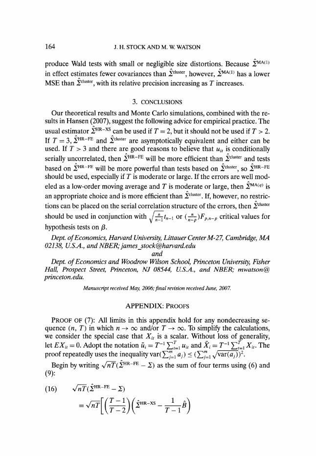
APPENDIX: PROOFS
PROOF OF (7): All limits in this appendix hold for any nondecreasing se- quence (n, T) in which n -- oo and/or T - o. To simplify the calculations, we consider the special case that Xi, is a scalar. Without loss of generality, let
EXit = O. Adopt the notation ui = T-1 =, ui and
_X
= T- Et X;,. The proof repeatedly uses the inequality
var(E='1 aj) < (E~j= v/ar(a1))2
Begin by writing ••(HR-FE
- ) as the sum of four terms using (6) and (9):
(16) 2/•(iHR-FE
_
,)
= -[(T- 2
IR T-1

HETEROSKEDASTICITY-ROBUST STANDARD ERRORS 165
T -12)(EHRxs
B)1 T-2 T-1
=
T•- 1 (HR-XS - EHR-XS) - T -2 B)
T-2) T-2
= T - 1) J(HR-XS - HR-XS) ( HR-XS - EIHR-XS)
T-2_ -(B - B) + N/:-(B
- B)
where XHR-XS is given in (8) and B is B given in (6) with ui, replaced by iit. The proof of (7) proceeds by showing that, under the stated moment condi-
tions, (a) ~/i-T(HR-XS
- EHR-XS) = Op(1),
(b) Vn/T(B - B) = OP(1/ /T),
(c) VT(~HR-XS - HR-XS) P 0, (d) vn/T(B^ - B) -4 0.
Substitution of (a)-(d) into (16) yields v/nT(XHR-FE - Z) = Op(1) and thus the result (7).
(a) From (8), we have that
var[,v/T (XHR-XS - EXHR-XS)]
[(
T -1AA-E(3- Ai2A~2Uit- ~2)
T-T var1 2
so (a) follows if it can be shown that var(T-1/2 t • tix
- -
1 1 X Ao 2AID3 + (AD2 + AD1
- 2A2A4
4 3 + A1AA2A3- 3
AIA2,
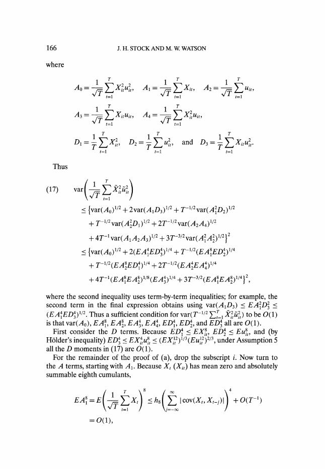
166 J. H. STOCK AND M. W. WATSON
where
1 T T1 rT1 T
jE Xlu 2 A =- EXi, A2=- ui
A?--- t=T
t1=1 t=1
1 1 T A3
-= vXituit, A4= -•
2it, t=1 t=l
1 1 1 D = T X"t, D2v DUitt2
and D3 =T XitA. t=l t=l t=l
Thus
(17) var 4T -2V
< {var(Ao)1/2 + 2var(A1D3)1/2 + T-1/2var(AD2 1/2
+ T-1/2var(A2D1 )1/2 + 2T-1/2var(A2A4)1/2
+ 4T-lvar(A1A2A3)1/2 + 3T-3/2var(AA 2)1/2}2
< {var(Ao)1/2 + 2(EAIED)1/4
+ T-1/2(EA ED)1/4
+ T-1/2(EA ED )1/4 + 2T-1/2(EA EA4 )1/4
? 4T-'(EA8EA)1/8 (EA4)1/4 + 3T-3/2 (EAEA8)1/4 }2
where the second inequality uses term-by-term inequalities; for example, the second term in the final expression obtains using var(AiD3) < EA2D <
(EAnED )1/2. Thus a sufficient condition for var(T-1/2 T=I
Xii) to be 0(1) is that var(Ao), EA8, EA 8, EA 4, EA 4, ED 4, ED 4, and ED4 all are 0(1).
First consider the D terms. Because ED4 < EXit,, ED4 < Eui, and (by
H5lder's inequality) ED 4< EXu4 8 < (EX t2)1/3(Eu1,2)2/3,
under Assumption 5 all the D moments in (17) are 0(1).
For the remainder of the proof of (a), drop the subscript i. Now turn to the A terms, starting with A1. Because Xt (Xit) has mean zero and absolutely summable eighth cumulants,
EA~= E -( X1 ) h,
cov(X/, Xt-)
+ O(T-1)
= O(1),
HETEROSKEDASTICITY-ROBUST STANDARD ERRORS 167
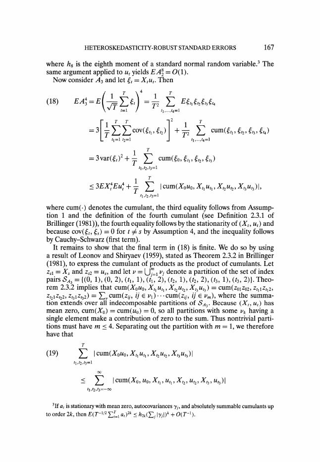
where h8 is the eighth moment of a standard normal random variable.3 The same argument applied to u, yields EA8 = 0(1).
Now consider A3 and let ,t
= Xu,. Then
(18) EA = E ,i
=T- E
Ett22t3
4
SE E t=1
tl,.... t4=1
=3COV( tl ,6+•t2 - c
t2, t3, t4
tl=1 t2=1 .t1,.....t4=l1
= 3var(,~)2 + cum(0, tl t2 )t3 tl,t2, t3=1
< 3EX4Eu4 + cum(X0u0, Xt1utl,
Xt2 Ut2, Ut3 )1, tl,t2,t3=1
where cum(.) denotes the cumulant, the third equality follows from Assump- tion 1 and the definition of the fourth cumulant (see Definition 2.3.1 of Brillinger (1981)), the fourth equality follows by the stationarity of (X,, u,) and because cov(:t, ,j) = 0 for t : s by Assumption 4, and the inequality follows by Cauchy-Schwarz (first term).
It remains to show that the final term in (18) is finite. We do so by using a result of Leonov and Shiryaev (1959), stated as Theorem 2.3.2 in Brillinger (1981), to express the cumulant of products as the product of cumulants. Let
Zs = Xs and Zs2 =
Us, and let v = UmI,
vj denote a partition of the set of index pairs SA3 = {(0, 1), (0, 2),
(tl, 1),
(tl, 2), (t2, 1), (t2, 2), (t3, 1), (t3, 2)}. Theo-
rem 2.3.2 implies that cum(Xo0u, Xt, ut, Xt2 Ut2, X3 Ut3) = cum(z01Z02, ZtllZtl2, z21lZt,2, Zt31Zt32) = Z.cum(zij, ij E V1)... cum(zij, ij E vm), where the summa- tion extends over all indecomposable partitions of SA3. Because (Xt, ut) has mean zero, cum(Xo) = cum(uo) = 0, so all partitions with some Vk having a single element make a contribution of zero to the sum. Thus nontrivial parti- tions must have m < 4. Separating out the partition with m = 1, we therefore have that
(19) I cum(X0u0, Xtu1lt, Xt2ut2, Xt3ut3) tl, t2, t3=1
SIcum(Xo, UO, Xtl u, UX, X 21, U ,t3],
Ut3) tl,t2, t3=-oo
3If at is stationary with mean zero, autocovariances yi, and absolutely summable cumulants up to order 2k, then E(T-1/2 tT=1 at)2k < h2k(Z] 1yj)k + O(T-1).
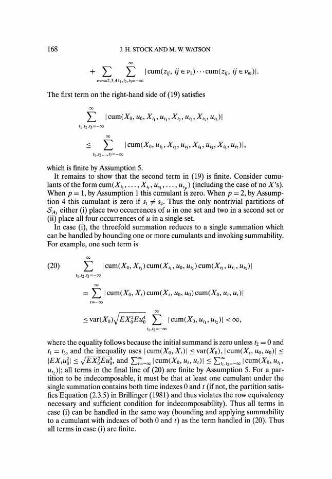
168 J. H. STOCK AND M. W. WATSON
+ Icum(zii, ij ev) ...cum(zi,
ij EiVm)I. v:m=2,3,4 tl, t2, t3=-oo
The first term on the right-hand side of (19) satisfies
E I cum(Xo, uO, XtUt, tu,,,
X2ut2, Xt3, u3) t1,t2,t3=-oo
00
< Y u Icum(Xo, ut, SX, uut3, S4X,4
ut5, X,6, uX,7 tl, t2,..., t7=-00
which is finite by Assumption 5. It remains to show that the second term in (19) is finite. Consider cumu-
lants of the form cum(Xt,,,..., Xtr, us, ..., us,) (including the case of no X's). When p = 1, by Assumption 1 this cumulant is zero. When p = 2, by Assump- tion 4 this cumulant is zero if sl 4 s2. Thus the only nontrivial partitions of SA3 either (i) place two occurrences of u in one set and two in a second set or (ii) place all four occurrences of u in a single set.
In case (i), the threefold summation reduces to a single summation which can be handled by bounding one or more cumulants and invoking summability. For example, one such term is
0O
(20) I cum(Xo, X3)cum(Xt1, uo, ut2) cum(Xt2, Utl, Ut3)I tl, t2, t3=-00
= Icum(Xo, Xt)cum(X,, U0, u0) cum(Xo, u0 , ut)1 t=-00
<var(Xo) EXgEu4
| Icum(Xo, ut, u'2)I <oc,
tl,t2=-00
where the equality follows because the initial summand is zero unless t2 = 0 and
tx = t3, and the inequality uses I cum(Xo, Xt)l < var(Xo), I cum(Xt, uo, uo) I
IEXtu _ /EX•Eu4, and
E=-o I cum(Xo, ut, u,)I
_ l
,2=- I cum(X0, ul, u,2)I; all terms in the final line of (20) are finite by Assumption 5. For a par-
tition to be indecomposable, it must be that at least one cumulant under the single summation contains both time indexes 0 and t (if not, the partition satis- fies Equation (2.3.5) in Brillinger (1981) and thus violates the row equivalency necessary and sufficient condition for indecomposability). Thus all terms in case (i) can be handled in the same way (bounding and applying summability to a cumulant with indexes of both 0 and t) as the term handled in (20). Thus all terms in case (i) are finite.
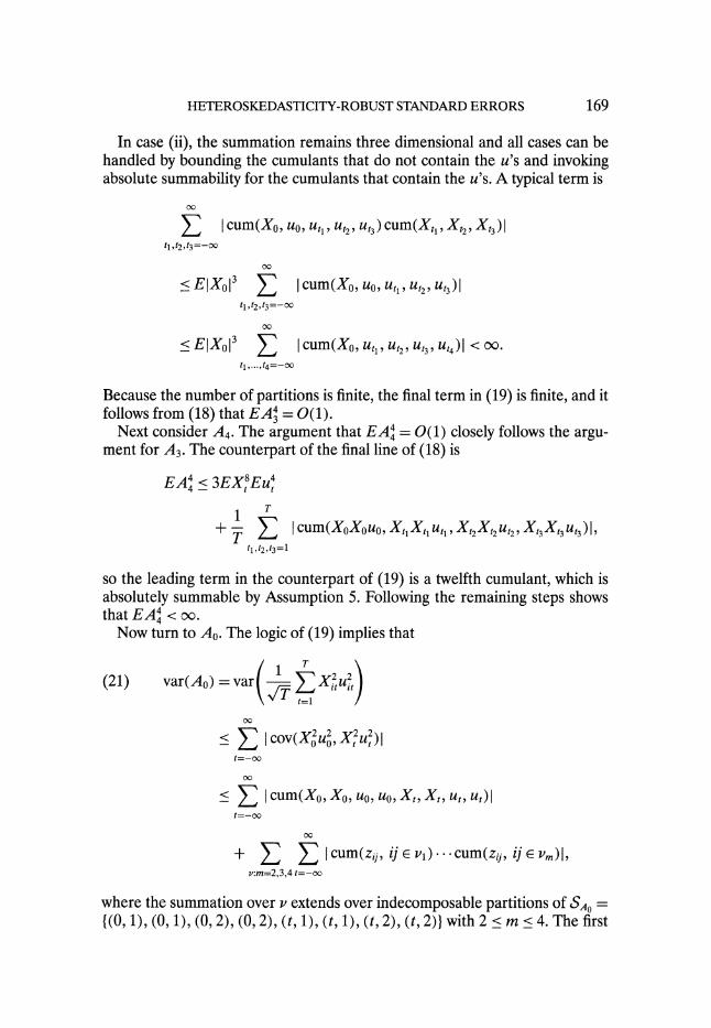
HETEROSKEDASTICITY-ROBUST STANDARD ERRORS 169
In case (ii), the summation remains three dimensional and all cases can be handled by bounding the cumulants that do not contain the u's and invoking absolute summability for the cumulants that contain the u's. A typical term is
L I cum(Xo, uo, ,,tl, u2,3)cum(Xtl,Xt2,9Xt3) tl, t2, t3= - o
< EXo?l3 | I cum(Xo, uo, ul, Ut2, t3)I
tl,t2, t3=-oo
0o
SEIXol3 | Icum(Xo, ut, ut2,ut3,u4)I <t00. tl,..., t4=-00
Because the number of partitions is finite, the final term in (19) is finite, and it follows from (18) that EA4 = 0(1).
Next consider A4. The argument that EA4 = 0(1) closely follows the argu- ment for A3. The counterpart of the final line of (18) is
EA4 < 3EXtEu4
+
T I cum(XoXouo, XtXt Ut,I, Xt2Xt2ut2,
Xt3Xt3ut3)I' t1,t2,t3=1
so the leading term in the counterpart of (19) is a twelfth cumulant, which is absolutely summable by Assumption 5. Following the remaining steps shows that EA 4< 00.
Now turn to A0. The logic of (19) implies that
(21) var(Ao) = vartjf X ui,
00
t=-00
00
< I cum(X0, X0, u0, u0, X,, X,, u,, u,)I t=-00oo
00
+ | Icum(z, ij v•v)--...cum(zi,
ij E vm), v:m=2,3,4 t=-00
where the summation over v extends over indecomposable partitions of SAo = {(0, 1), (0, 1), (0, 2), (0, 2), (t, 1), (t, 1), (t, 2), (t, 2)} with 2 < m < 4. The first
170 J. H. STOCK AND M. W. WATSON
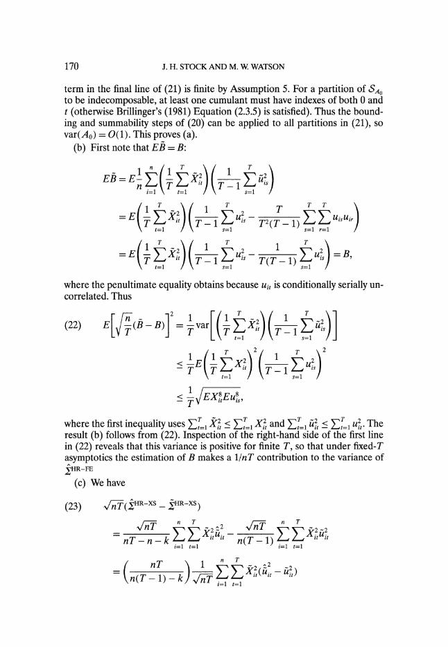
term in the final line of (21) is finite by Assumption 5. For a partition of SAo to be indecomposable, at least one cumulant must have indexes of both 0 and t (otherwise Brillinger's (1981) Equation (2.3.5) is satisfied). Thus the bound- ing and summability steps of (20) can be applied to all partitions in (21), so var(Ao) = 0(1). This proves (a).
(b) First note that EB = B:
1 n(! T1 Y U TT E_-) EB = E-X;Y s
ni=1 t=l s=l
T it
T-1 Uis T2(T-
1)
s il r
r ST2 (T ) UisUir
t=1 s= 1 r=1
( T T2 T 2
1 f,2 T- 1 Uis
T(T1- 1) Uis=B,
t=l s=l s=1
where the penultimate equality obtains because ui, is conditionally serially un- correlated. Thus
(22) E ( (B-B) -var X t) ( is t=1 1
<- EXfEu,
T- T T -'1
where the first inequality uses ET12 _
= Ei 1 X2t and T1, it - Et= uit. The
result (b) follows from (22). Inspection of the right-hand side of the first line in (22) reveals that this variance is positive for finite T, so that under fixed-T asymptotics the estimation of B makes a 1/nT contribution to the variance of JHR-FE
(c) We have
(23) /nT((HR-XS
_
,HR-XS) n T 2 n T
2 - T- - k n(T-1)
InT n T1 2 T k L2(TlEit i
n(T - 1) - k) • /=1 tl
HETEROSKEDASTICITY-ROBUST STANDARD ERRORS 171
n(T - 1) - k
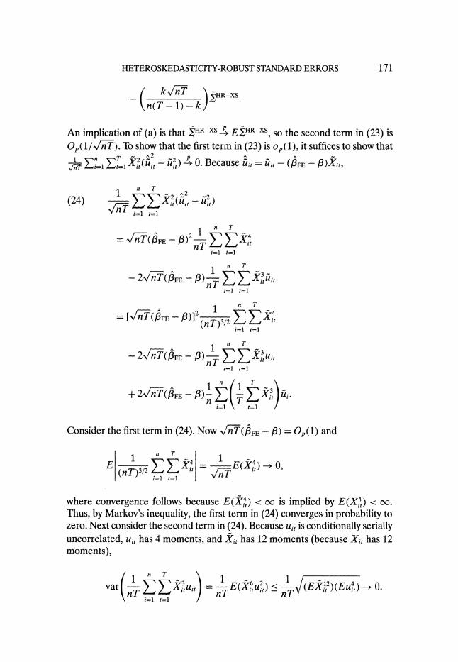
An implication of (a) is that XHR-XS 4 E•HR-XS, SO the second term in (23) is
O,(1/V1T). To show that the first term in (23) is o,(1), it suffices to show that 1
n ,2T 2,
nEi ET=1
X(~lit,
- i2-), 0. Because it = Ui - (FE -t )Xt,
n nT
(24) "2 E/
E i=
i t=l
(it -Ut
n T
"-- %-•(FE
-
9)2_.
nT
i=1 t= 1
2 In--T(FE --0•) •-T E ES3it i=1 t=1
-
2• (3FEp - 1 , "Tu,
i=1 t=1
1 n T
- 2•
(FFE - ) X1 itn t i=1 t=1
Consider the first term in (24). Now V/n(I3FE - -3)
= O,(1) and
1 1 E XF =
'- E(Xi)
-
? S(nT)3/2 i==1 t=
where convergence follows because E(Xit)
< c is implied by E(X4) < 0.
Thus, by Markov's inequality, the first term in (24) converges in probability to zero. Next consider the second term in (24). Because ui, is conditionally serially uncorrelated, ui, has 4 moments, and
Xit has 12 moments (because Xit has 12
moments),
var (••
1 tl
uit) E(=ut)
1 (E 2)(u) .
172 J. H. STOCK AND M. W. WATSON
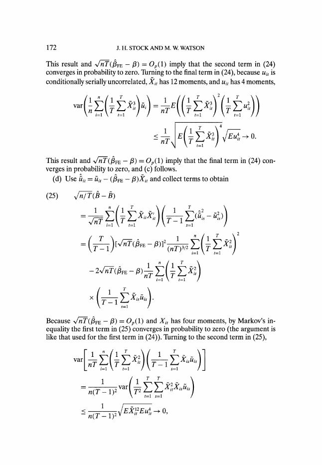
This result and (-nT(FE - P) = Op(1) imply that the second term in (24)
converges in probability to zero. Turning to the final term in (24), because ui, is
conditionally serially uncorrelated, Xi, has 12 moments, and ui, has 4 moments,
1( n 1 ) 1 (( Tt21 var X t u -- E X -
Uit i=1 t=l t=l t=l
< NE X -Eit
0. -nt=
This result and V/-T(IFE - /3) = Op(1) imply that the final term in (24) con-
verges in probability to zero, and (c) follows.
(d) Use uit = it- (IFE - P)Xi and collect terms to obtain
(25) \n-T( -3B)
1 t
1 A 1
i=1 t=1 s=1 1 )
n 1
T- 2Vn(3FE
- ) )/2i= t=l i=1
" t=l
1 1 x
1 E X is Uis s=-1
Because V-T(IFE - /3) = Op(1) and Xit has four moments, by Markov's in- equality the first term in (25) converges in probability to zero (the argument is like that used for the first term in (24)). Turning to the second term in (25),
1 1n2T
T
n(-va 1)2r ir itis Uis i=1T t= l s=l
1 EXE~12 -4
n(T-t=1)2 s=it
it 7 X' V'
~
HETEROSKEDASTICITY-ROBUST STANDARD ERRORS 173
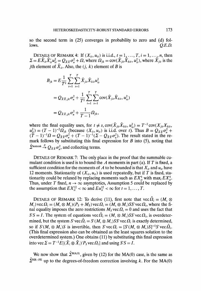
so the second term in (25) converges in probability to zero and (d) fol- lows. Q.E.D.
DETAILS OF REMARK 4: If (Xit, uit) is i.i.d., t = 1,..., T, i = 1,..., n, then = EX Xi,,u =
Qit- o-2 + f2, where f2jk = COv(XjitXkit, U2t), where Xjit is the
jth element of Xit. Also, the (j, k) element of B is
Bjk = T2 XjitXkitUis
t=1 s=1
= Qk,Ijko +COv(TXitXkitX uIs t=1 s=1
where the final equality uses, for t : s, cov(XitXkit u) T-2 COv(XjitXkit, u2) = (T - 1)-2 jk (because (Xi,, ui,) is i.i.d. over t). Thus B = Q eo2 + (T - 1)-1' = QXXko,2 + (T - 1)-1(, - Qf o-u2). The result stated in the re- mark follows by substituting this final expression for B into (5), noting that
Shomosk _4_ Qj o,2,
and collecting terms.
DETAILS OF REMARK 7: The only place in the proof that the summable cu- mulant condition is used is to bound the A moments in part (a). If T is fixed, a sufficient condition for the moments of A to be bounded is that Xit and uit have 12 moments. Stationarity of (Xit, uit) is used repeatedly, but if T is fixed, sta- tionarity could be relaxed by replacing moments such as EX4, with maxt EX4t,. Thus, under T fixed, n --+ o asymptotics, Assumption 5 could be replaced by the assumption that EXL12 < 00 and EU12 <00 cfor t = 1, ..., T.
DETAILS OF REMARK 12: To derive (11), first note that vecf2i = (M, 0
M,)vecif2 = (M, 0 M,)(Ps + Ms)vec;i = (M, 0 M,)SS'vec i, where the fi-
nal equality imposes the zero restrictions Ms vec i = 0 and uses the fact that S'S = I. The system of equations vecfi = (M, 0 M,)SS'vec;i, is overdeter- mined, but the system S'vec i = S'(M, 0 M,)SS'vec 2i is exactly determined, so if S'(M, 0 M,)S is invertible, then
S'vec2/i = [S'(M, 0 M,)S]-lS'vecf2i.
(This final expression also can be obtained as the least squares solution to the overdetermined system.) One obtains (11) by substituting this final expression into vec = T-1E[(Xi 0 Xi)'Psvec1i] and using S'S = I.
We now show that IMA(0), given by (12) for the MA(0) case, is the same as
?HR-FE up to the degrees-of-freedom correction involving k. For the MA(0)
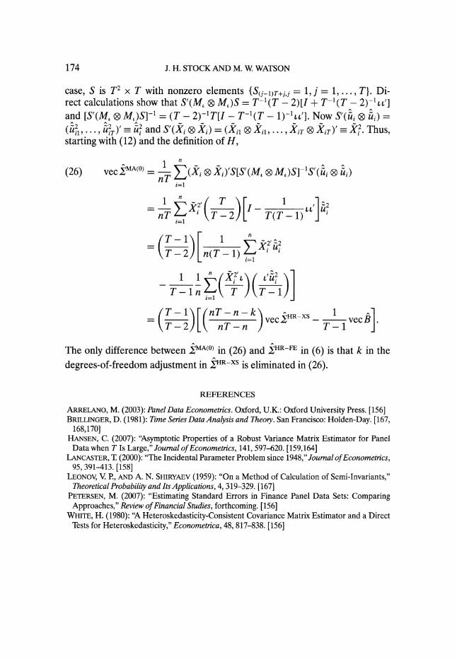
174 J. H. STOCK AND M. W WATSON
case, S is T2 x T with nonzero elements {S(j-1)T+j,j = 1, j = 1, ..., T}. Di- rect calculations show that S'(M, 0 M)S = T-1(T - 2)[I + T-I(T - 2)-1LL'] and [S'(M, 0 M,)S]-1 = (T - 2)-1'T[I - T-1(T - 1)-1~']. Now S'(ii 0 ii) =
(ui, ..., U\-. uf and S'(Xi 9 X) = ( 91 Xil, ... ,XiT 9 XiT) •
i2. Thus, starting with (12) and the definition of H,
(26) vec MA(0)
= i i (X X)'S[S'(M, M,)S]-ls'(ii, &i) i=1
1 T 1
nT 2 T -2)[ T(T - 1) c
2
( T - 1 1
n
ki U
T--2)
n(T- 1)(1
T-ln i T T -1)
/T-1 nT-n-kv -vec = -
2
InT
nT- )vecHR-XS 1vecBi T-2 nT-n T-1
The only difference between 1MA(0) in (26) and XHR-FE in (6) is that k in the
degrees-of-freedom adjustment in XHR-XS is eliminated in (26).
REFERENCES
ARRELANO, M. (2003): Panel Data Econometrics. Oxford, U.K.: Oxford University Press. [156] BRILLINGER, D. (1981): Time Series Data Analysis and Theory. San Francisco: Holden-Day. [167,
168,170] HANSEN, C. (2007): "Asymptotic Properties of a Robust Variance Matrix Estimator for Panel
Data when T Is Large," Journal of Econometrics, 141, 597-620. [159,164] LANCASTER, T. (2000): "The Incidental Parameter Problem since 1948," Journal ofEconometrics,
95, 391-413. [158] LEONOV, V. P., AND A. N. SHIRYAEV (1959): "On a Method of Calculation of Semi-Invariants,"
Theoretical Probability and Its Applications, 4, 319-329. [167] PETERSEN, M. (2007): "Estimating Standard Errors in Finance Panel Data Sets: Comparing
Approaches," Review of Financial Studies, forthcoming. [156] WHITE, H. (1980): 'A Heteroskedasticity-Consistent Covariance Matrix Estimator and a Direct
Tests for Heteroskedasticity," Econometrica, 48, 817-838. [156]