Flexible Monitoring of Storage I/O

Flexible Monitoringof Storage I/O

by

Tim Benke

A thesispresented to the University of Waterloo

in fulfillment of thethesis requirement for the degree of

Master of Mathematicsin

Computer Science

Waterloo, Ontario, Canada, 2009

c© Tim Benke 2009

I hereby declare that I am the sole author of this thesis. This is a true copy of thethesis, including any required final revisions, as accepted by my examiners.

I understand that my thesis may be made electronically available to the public.

ii

Abstract

For any computer system, monitoring its performance is vital to understandingand fixing problems and performance bottlenecks. In this work we present thearchitecture and implementation of a system for monitoring storage devices thatserve virtual machines. In contrast to existing approaches, our system is moreflexible because it employs a query language that can capture both specific anddetailed information on I/O transfers. Therefore our monitoring solution providesthe user with enough statistics to enable him or her to find and solve problems, butnot overwhelm them with too much information. Our system monitors I/O activityin virtual machines and supports basic distributed query processing. Experimentsshow the performance overhead of the prototype implementation to be acceptablein many realistic settings.

iii

Acknowledgements

I would like to thank my supervisors Professor Martin Karsten and ProfessorKenneth Salem for their patience and great support. I would also like to thankOguzhan Ozmen, Umar Farooq, Patrick Kling and Jeff Pound for having an openear for my problems. I thank Professor Ashraf Aboulnaga and Professor Johnny W.Wong for being my thesis readers. I also want to thank the staff of the Universityof Waterloo for making this possible.

iv

Dedication

This is dedicated to Maewen.

v

Contents

List of Tables viii

List of Figures ix

1 Introduction 1

2 Background 4

2.1 I/O Monitoring Tools . . . . . . . . . . . . . . . . . . . . . . . . . . 4

2.2 Virtual Machine Monitor . . . . . . . . . . . . . . . . . . . . . . . . 6

2.2.1 Operating System-level Virtualization . . . . . . . . . . . . . 7

2.2.2 Hardware Virtualization . . . . . . . . . . . . . . . . . . . . 8

2.2.3 Software-assisted Full Virtualization . . . . . . . . . . . . . . 8

2.2.4 Paravirtualization . . . . . . . . . . . . . . . . . . . . . . . . 8

2.2.5 Hardware-assisted Full Virtualization . . . . . . . . . . . . . 9

2.2.6 Hybrid Virtualization . . . . . . . . . . . . . . . . . . . . . . 9

2.2.7 The Xen VMM . . . . . . . . . . . . . . . . . . . . . . . . . 10

2.2.8 Xen Blocktap . . . . . . . . . . . . . . . . . . . . . . . . . . 10

2.3 Data Stream Management System . . . . . . . . . . . . . . . . . . . 14

2.3.1 DSMS Query Languages . . . . . . . . . . . . . . . . . . . . 15

2.3.2 DSMS Optimization/Plan Generation . . . . . . . . . . . . . 15

3 System Design 17

3.1 System Organization . . . . . . . . . . . . . . . . . . . . . . . . . . 17

3.2 Data Model . . . . . . . . . . . . . . . . . . . . . . . . . . . . . . . 20

3.2.1 Timestamps . . . . . . . . . . . . . . . . . . . . . . . . . . . 22

3.2.2 Request ID . . . . . . . . . . . . . . . . . . . . . . . . . . . 23

vi

3.2.3 Categorical Fields . . . . . . . . . . . . . . . . . . . . . . . . 23

3.2.4 Other Numerical Fields . . . . . . . . . . . . . . . . . . . . . 23

3.3 Extending Blocktap . . . . . . . . . . . . . . . . . . . . . . . . . . . 23

3.4 Extending STREAM . . . . . . . . . . . . . . . . . . . . . . . . . . 24

3.5 Monitoring Queries . . . . . . . . . . . . . . . . . . . . . . . . . . . 24

3.5.1 Query 0: Baseline Query . . . . . . . . . . . . . . . . . . . . 25

3.5.2 Query 1: Filter Specific I/O Requests . . . . . . . . . . . . . 25

3.5.3 Query 4: Response Times . . . . . . . . . . . . . . . . . . . 25

3.5.4 Query 8: Filter Tuples with High Response Time . . . . . . 27

4 Experimental Results 30

4.1 Overview of Experiments . . . . . . . . . . . . . . . . . . . . . . . . 30

4.2 Experimental Testbed . . . . . . . . . . . . . . . . . . . . . . . . . 30

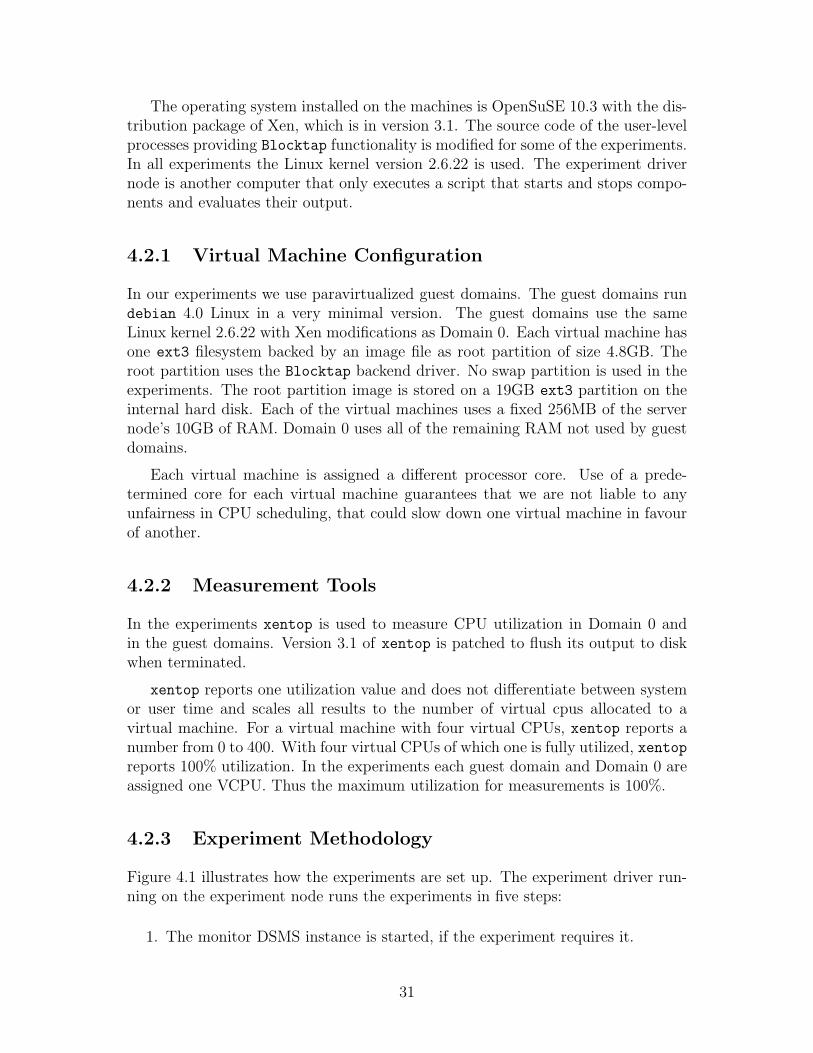
4.2.1 Virtual Machine Configuration . . . . . . . . . . . . . . . . . 31

4.2.2 Measurement Tools . . . . . . . . . . . . . . . . . . . . . . . 31

4.2.3 Experiment Methodology . . . . . . . . . . . . . . . . . . . . 31

4.3 Experiments . . . . . . . . . . . . . . . . . . . . . . . . . . . . . . . 32

4.3.1 Experiment 1: Overhead of Tracing I/O Tuples . . . . . . . 33

4.3.2 Experiment 2: Impact of Query Complexity . . . . . . . . . 34

4.3.3 Experiment 3: Parallel Query Execution Scalability . . . . . 36

4.3.4 Experiment 4: Impact of Offloading on Utilization . . . . . . 37

4.3.5 Experiment 5: Effect of Filtering . . . . . . . . . . . . . . . 39

4.3.6 Experiment 6: Virtual/Physical Machine Scalability . . . . . 40

5 Conclusions and Future Work 44

5.1 Conclusions . . . . . . . . . . . . . . . . . . . . . . . . . . . . . . . 44

5.2 Future Work . . . . . . . . . . . . . . . . . . . . . . . . . . . . . . . 44

Appendix 46

References 53

vii

List of Tables

3.1 Record Schemata at Various Points in the Monitoring System . . . 21

3.2 Filter STREAM input example . . . . . . . . . . . . . . . . . . . . . . 21

3.3 Query 1 Sample Input . . . . . . . . . . . . . . . . . . . . . . . . . 26

3.4 Query 1 Sample Output . . . . . . . . . . . . . . . . . . . . . . . . 26





viii

List of Figures

1.1 Problem Setting . . . . . . . . . . . . . . . . . . . . . . . . . . . . . 2

2.1 IO Ring . . . . . . . . . . . . . . . . . . . . . . . . . . . . . . . . . 11

2.2 Blocktap Modes [45] . . . . . . . . . . . . . . . . . . . . . . . . . . 13

3.1 I/O Monitoring Architecture . . . . . . . . . . . . . . . . . . . . . . 18

3.2 Guest Domain . . . . . . . . . . . . . . . . . . . . . . . . . . . . . . 18

3.3 Server Node Domain 0 . . . . . . . . . . . . . . . . . . . . . . . . . 19

3.4 Server and Monitor Node . . . . . . . . . . . . . . . . . . . . . . . . 20

3.5 Query 1 . . . . . . . . . . . . . . . . . . . . . . . . . . . . . . . . . 25

3.6 Query 4 . . . . . . . . . . . . . . . . . . . . . . . . . . . . . . . . . 26

3.7 Query 8 . . . . . . . . . . . . . . . . . . . . . . . . . . . . . . . . . 28

4.1 Execution of Experiments . . . . . . . . . . . . . . . . . . . . . . . 32

4.2 Results of Experiment 1 . . . . . . . . . . . . . . . . . . . . . . . . 34



4.5 Distributed Configurations . . . . . . . . . . . . . . . . . . . . . . . 38


4.7 Configuration with Filter Query . . . . . . . . . . . . . . . . . . . . 40

4.8 Filter Query . . . . . . . . . . . . . . . . . . . . . . . . . . . . . . . 40



1 Query 2: Sum of the Size of I/O Requests . . . . . . . . . . . . . . 46

2 Query 3: Interarrival Times . . . . . . . . . . . . . . . . . . . . . . 47

3 Query 5: Percentage of Sequential Requests . . . . . . . . . . . . . 48

ix

4 Query 6: Variance of Request Sizes . . . . . . . . . . . . . . . . . . 49

5 Query 7: Histogram of Starting Sectors . . . . . . . . . . . . . . . . 50

6 Query 9: Number of Unresolved Requests . . . . . . . . . . . . . . 50

7 Query 10: iostat for Xen . . . . . . . . . . . . . . . . . . . . . . . . 51

8 Query 10M: iostat for Xen on the monitor node . . . . . . . . . . . 52

x

Chapter 1

Introduction

System monitoring enables the user to find performance bottlenecks, detect failuresor anomalies, tune the system’s performance, automate resource allocation, char-acterize a workload, and build models of the system. The New Oxford AmericanDictionary [34] defines monitoring as:

1. observe[ing] and check[ing] the progress or quality [of a system]over a period of time

2. keep[ing] [a system] under systematic review

We are focussing on monitoring storage devices, such as disk drives. Computerstransfer data between disks and memory using requests and responses. Requeststell the disk where data should be written to or read from. Conversely, the disksignals completion of requests with responses. This work presents a system tomonitor requests and responses and measure performance statistics.

The objective of I/O monitoring is to keep track of I/O statistics for administra-tors or automated administrative tools. Examples of questions that administratorsmight ask are how high the throughput of a particular physical disk is, what themean and maximum response time of disk requests is, how many requests are reador write requests, or how the response times are distributed.

Existing approaches for I/O monitoring can be classified as event-driven orsampling [27] monitors. The former activate exactly when an I/O-related eventhappens while the latter only activate periodically. Relevant events are the issuanceand the completion of requests.

Similarly, Jain classifies the presentation of results in two categories: onlineand batch [27]. Online monitors either display the results continuously or at fre-quent intervals, while batch monitors amass data that another program can analyselater. Alternatively, the terms off-line or periodic are used for batch, and rolling issometimes used to mean online.

1

Another classification of monitors is based on whether a user can customizewhat is monitored and displayed for a particular use. Some monitors offer a rigidset of statistics to the user while customizable monitors enable a user to procure atheoretically infinite number of statistics.

The approach presented in this thesis is event-driven, online, and customizable.This is in contrast to existing monitoring solutions which are often sampling-based,online and rigid. The popular UNIX tool iostat is an example of such a monitorwhile approaches that use tracing capabilities in the kernel, such as DTrace [17],can be classified as event-driven and online monitors. DTrace also offers simplefilter capabilities and is thus customizable, but cannot directly aggregate resultsacross machines. DTrace is compared to our approach in more detail in Section2.1.

Another popular method is to trace events in an event-driven batch monitor toperform analysis later. Then the analysis can in principle compute any statisticon the data. For some monitoring tasks administrative tools require a real-timeanalysis, for instance to raise alarms or control available resources. This rendersbatch monitors useless for real-time monitoring.

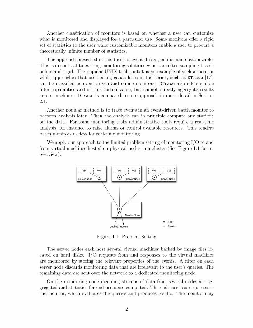
We apply our approach to the limited problem setting of monitoring I/O to andfrom virtual machines hosted on physical nodes in a cluster (See Figure 1.1 for anoverview).

Monitor Node

Server Node

VM VM

*

Server Node

VM VM

*

Server Node

VM VM

*

+

Queries Results +*FilterMonitor

Figure 1.1: Problem Setting

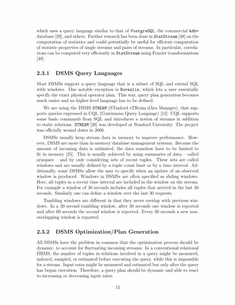
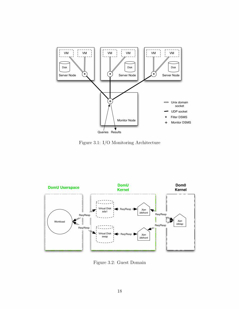
The server nodes each host several virtual machines backed by image files lo-cated on hard disks. I/O requests from and responses to the virtual machinesare monitored by storing the relevant properties of the events. A filter on eachserver node discards monitoring data that are irrelevant to the user’s queries. Theremaining data are sent over the network to a dedicated monitoring node.

On the monitoring node incoming streams of data from several nodes are ag-gregated and statistics for end-users are computed. The end-user issues queries tothe monitor, which evaluates the queries and produces results. The monitor may

2

split user queries into two parts: a filter query to be executed at one or more servernodes, and a residual query to execute at the monitor node.

The advantage of this architecture is that by using distributed aggregation fromseveral machines, we are able to centrally monitor groups of computers. The queryinterface presents the end-user with a flexible and easy to use access to monitoreddata. To implement this distributed architecture, we have had to answer severalquestions:

Where and how to measure request properties?

To trace I/O requests we have to use a hook in one of the software layers throughwhich I/O requests pass. The different layers are the application layer, operatingsystem layer, and the virtual machine layer. We are taking advantage of existinghooks in the I/O interface for virtual machines. Using a wrapper, requests areforwarded to a database on the server node.

We have chosen to trace at the virtual machine level because virtualization playsan important role in data centres as physical machines are migrated to virtual ma-chines to save energy and cooling costs. Resources are constrained and monitoringthe performance is essential, e.g., for testing new applications. Virtualization tech-nology is widely used. The Xen virtualization machine monitor (VMM), which weare using, already includes hooks for monitoring I/O events.

What statistics to measure?

Rather than producing predefined statistics, we provide customizability by al-lowing clients to define statistics of interest to them. As described in Section 2.3 weuse a data stream management system (DSMS) [13] to provide this customizability.

To summarize, this work contributes the following:

1. An architecture for distributed, customizable I/O monitoring, and a prototypeimplementation of that architecture.

2. Experimental analysis of the overhead associated with monitoring. It turnsout that the overhead of flexible statistics may be high, but by calculatingstatistics on a separate monitor node, the performance impact on the servernodes can be minimized.

3. Experimental analysis of filtering mechanisms at the server nodes. Thisdemonstrates that the volume of data sent to the monitor node can be reducedwith little impact on the server nodes.

In Chapter 2, background material for this work is given. Chapter 3 explains thesystem. Chapter 4 presents the experimental methodology and results. Conclusionsand future work are described in Chapter 5.

3

Chapter 2

Background

2.1 I/O Monitoring Tools

Tools that monitor I/O activity try to store the equivalent of the “header” of I/Orequests and the times at which they are issued, worked on and completed. Whichof these properties are recorded and the granularity at which they are recordeddepend on the specific tool. Currently there are several disk I/O monitoring toolsavailable for use in production systems.

iostat is a simple UNIX tool for basic disk I/O monitoring. In its Linuximplementation iostat is only about 500 lines of code. It is “monitoring deviceloading by observing the time the devices are active in relation to their averagetransfer rates” according to its manual page [30]. I/O statistics, such as the timethat a device is active and its transfer rates, are obtained through the kernel’spseudo-filesystem procfs.

procfs makes information from the kernel’s internals available to user programs.Available are counters for issued read and write requests, completed requests, andsmall requests merged into large requests. Other counters keep track of time spenton reading, writing, and performing I/O requests as well as the number of currentlyoutstanding requests. The values are updated when an I/O event occurs or aprogram reads the pseudo-file containing the counters. All of these counters areavailable per physical disk and some of the request counters are also available forindividual partitions.

iostat and other simple monitoring tools that compute statistics based on thesecounters have an insignificant performance impact because of their limited power.procfs and iostat do not provide information on individual requests, such as theirlocation on disk or size. Furthermore, it is not possible to obtain statistics, such asvariances or quantities other than averages.

Generally, the arithmetic mean may often not suffice as a statistic. As anexample consider a workload consisting of 50% very small write requests and 50%very large write requests. If the throughput of this workload were low it would not

4

be visible in the arithmetic mean of the requests sizes. In this case it would beuseful to look at a histogram of the request sizes to see this imbalance.

Many other tools offer the same limited I/O statistics and some have a moreaccessible or usable presentation of these statistics. collecti [21] is one of them. Itshows all of iostat’s statistics and uses the same information available in procfs.Aside from a command-line interface it can directly convert measured data to adiagram or csv-file.

If tools do not get information from procfs, they usually instrument the ker-nel themselves. Some tools like fs usage that is available for Mac OS X can tracefilesystem related system calls and page faults for specific processes [31]. A moregeneral version called sc usage traces all system calls [32]. For Linux, strace

does the same job. These tracing instruments record which system call was exe-cuted with what parameters, but not how the kernel fulfills the actual I/O request.Moreover, the data generated this way may become overwhelming very quicklyand a significant performance penalty may be incurred as the data are collected.Moreover strace only works on a per-process basis.

A more powerful and flexible tool is SUN’s DTrace [17]. DTrace instrumentsthe kernel and user programs with so-called probes. In contrast to strace, it canmonitor individual processes or the kernel or a whole system. It provides the userwith a query interface to specify what DTrace should do when a probe is activated.It can compute or print expressions based on the values collected by the probe whenit is activated. It features a C-like programming language with awk-like predicatesand it has the following built-in aggregation functions: sum, count, maximum,average, minimum and histograms.

DTrace scripts are compiled in user-space and transferred to the DTrace virtualmachine in the kernel. Probes belong to a so-called provider that registers withthe DTrace virtual machine. Examples of providers are io for I/O-related probesor syscall for system calls. A more fine-grained monitoring is available with thefunction boundary testing (fbt) provider; it offers probes for the entry and exit ofevery kernel function.

To monitor hard disk I/O, the io provider has access to most of the relevantinformation available. DTrace can relate an I/O request to the corresponding file,process, and device. For each request its file name, path, and offset are available.The process id and the process’s file and path can be procured as well as the majorand minor number of the used device. More detailed information like the request’sstart and completion time, if it is a read or write request and if it is synchronousor not, are available, too.

DTrace offers support for simple filtering. It is available for Solaris, Mac OSX and FreeBSD. An analogous project called SystemTap is under development forLinux, but not yet in a stable state.

DTrace is not trying to address all of the same issues as our approach is. It is alow-level source for monitoring data similar to our approach that logs information

5

from the I/O to and from virtual machines. In addition to that it is able to tracemany more different types of events and to perform some filtering on the collecteddata. It runs in a virtual machine in the kernel and while our source of information isthe VMM, most filtering and processing is performed on the user-level. In additionto DTrace’s capabilities, our approach can provide distributed aggregation of I/Otraces from several machines and can also perform potentially more complicatedprocessing without any concerns of decreasing the operating system performance.Within our architecture it would be possible to use DTrace as an alternative meansof collecting I/O event information from individual server nodes.

VMware has developed a similar service for monitoring virtual machines calledVProbes [42]. It is part of the current versions of VMware Workstation and VMwareFusion. Expressions and functions are written in a Lisp-like language, but moreconstrained than DTrace. It can record start and finish times of I/O requests aswell as the operation performed and their size and location on the virtual disk.

VProbes shares the essentially same source into I/O transfers as our approachbut not the same privilege level of filtering and processing. The database we areusing runs on the user-level as opposed to VProbes and DTrace that run in theVMM and the operating system kernel. Moreover expressions in VProbes are evenmore limited than in DTrace because of technical limitations of the VMM.

2.2 Virtual Machine Monitor

Virtualization is the abstraction of an operating system from its underlying physicalhardware. A familiar analogy is how operating systems offer abstraction from thehardware. Without this abstraction each process would have to directly commu-nicate with the hardware and only one process could run at a time. An operatingsystem allows processes to share the underlying hardware. In addition, it abstractsfrom the given hardware and offers a more general interface to the devices. Forexample, each different model of a network interface card uses different chips andcircuits but a driver in the operating system offers one general interface to the op-erating system that is used to present an even simpler socket interface to the user.Multiplexing and time-sharing of the hardware are other abilities of the operatingsystem. The scheduler allocates a share of the processor’s time to each process,so more than one process can be run on one processor concurrently. When severalprocesses want to use the same network interface card and send packets over thenetwork, the operating system multiplexes the packets and allocates each processa share of the network interface card’s bandwidth.

Similarly, adding virtualization between the hardware and the operating systemallows one to simultaneously run more than one operating system on the virtualizedresources. A virtual machine monitor (VMM), or hypervisor, is the component thatimplements this abstraction layer. Some of the reasons for virtualization are thesame as for operating systems, e.g., higher utilization of CPU and devices. In

6

addition, VMMs offer improved performance isolation, and the ability to migratevirtual machines between VMMs on different machines, which results in higheravailability and security. By using so-called virtual appliances – simple virtualmachines serving a single purpose – failures of user software and operating systemscan be isolated in a virtual machine and do not affect other services on the samephysical machine [14]. By replacing several under-utilized physical machines withvirtual machines managed by a VMM, maintenance costs and power consumptioncan be reduced. This is important because according to the US EnvironmentalProtection Agency the power consumption of data centres is increasing rapidly[10].

There are several VMMs available. Microsoft [3], Parallels [5], VMware [41],XenSource [14], Sun [7], IBM [8], and many others have developed virtualization so-lutions. Notable open-source VMMs are Bochs [1], KVM [39], OpenVZ [4], QEMU[15], User Mode Linux [22] and Xen [14]. We focus on the VMM Xen, because itis open-source and it provides software device drivers, which have direct access tothe I/O events. First we give an overview of different approaches to virtualization,and then we focus on Xen and how it handles disk I/O in particular.

2.2.1 Operating System-level Virtualization

Instead of virtualizing a whole machine, the operating system kernel usually staysthe same but different isolated user-spaces are made available. Each user-spaceinstance – sometimes called container – appears as an independent machine to theuser. In contrast to this, the OS-level virtualization solution Solaris Zones [38]offers the ability to host different Solaris kernels and Linux distributions.

Because it is less flexible, this solution only results in a small performance im-pact. For Linux, OpenVZ provides Operating System-level virtualization. OpenVZis the basis for Parallels commercial product Virtuozzo. Another example of OS-level virtualization is FreeBSD Jails [28]. Both approaches share the property thatthe original operating system’s kernel is serving multiple containers. Therefore thisapproach is limited to running only one type of operating system. The differentcontainers can be limited in their access to the hosting operating system. Addi-tionally some approaches allow the administrator to schedule the resources amongthe containers.

Because of the tight coupling between virtual machines and the hosting oper-ating system, these approaches can often offer high performance. One of the dis-advantages at least of OpenVZ’s solution is that it offers less performance isolationbetween the different operating system instances in comparison to software-assistedfull virtualization and paravirtualization approaches [33].

7

2.2.2 Hardware Virtualization

Before the x86 architecture became successful IBM had already produced virtu-alization solutions. This had been done on special versions of the S/360 andS/370 architecture [20]. Unfortunately the x86 architecture is not easily virtu-alizable. Popek and Goldberg [37] have put forward universal requirements forwhat is needed to virtualize any processor architecture. One of the requirementsis that any instruction that changes the configuration of the machine should beexecuted in privileged mode, or trap if it is not. Unfortunately the x86 architec-ture has 17 instructions that do not fulfill this requirement [20]. Several differentvirtualization approaches try to solve this problem in different ways. The solutionsinclude software-assisted full virtualization, hardware-assisted full virtualization,and paravirtualization. They are described in the following subsections.

2.2.3 Software-assisted Full Virtualization

This technique is also called binary translation or binary rewriting [20]. The se-quence of instructions until the next jump instruction is scanned for any of theunsafe instructions in the x86 instruction set. Each such instruction is marked andemulated when it is reached. After each jump the next sequence of instructions isscanned and marked if necessary [20].

This scanning and replacement of instructions often makes this approach slowerthan other approaches. An advantage of binary rewriting is that the VMM can rununmodified guest operating systems.

2.2.4 Paravirtualization

The term paravirtualization has been used first in connection with the operatingsystem Denali [46]. Denali and later Xen [14] use this technique to support virtu-alization even on the x86 architecture. Unlike Denali, which only hosts single-usersingle application operating systems, Xen hosts a general-purpose multi-user oper-ating system [14].

For paravirtualization, parts of the operating system have to be ported for thespecific VMM. One example is very simple generic drivers that replace device driversfor specific hardware models. This absolves the VMM from offering complicatedimplementation or emulation of these device drivers. Because the paravirtualizedoperating systems are aware that they are running in a virtual machine, they canbe specifically optimized for virtualization. The clock, for example, can be han-dled better, because the kernel can be modified to not continually expect timerinterrupts. This is useful if a virtual machine has to keep track of time even if itis not always running. In comparison to software-assisted and hardware-assistedfull virtualization, the performance of devices can be much better because those

8

approaches have to emulate devices. In this work we are exclusively using paravir-tualized guest domains.

2.2.5 Hardware-assisted Full Virtualization

Software-assisted full virtualization and paravirtualization solutions have increasedthe interest in x86 virtualization. Thus, AMD and Intel have recently begun toadd virtualization extensions and corrections to x86 processors. Some of the afore-mentioned virtualization software projects can take advantage of some of these newprocessor extensions although their original approach was purely software-assistedor paravirtual.

With support from these processor extensions, it is possible to support fullvirtualization without modifying the operating system or using binary rewriting.There are many performance advantages of this approach, but one disadvantagein comparison to paravirtualized machines is the more complicated emulation ofvirtual device drivers.

The drivers in a virtualization-unaware operating system have been writtenfor a specific hardware. Thus this hardware has to be emulated by the VMM. Toaccomplish this emulation, any communication from the actual driver that interactswith the hardware has to be first translated to an intermediate simple interface andthen back to the specific interface the driver in the guest domain expects. Thereforehardware-assisted solutions can sometimes not achieve the same I/O throughputas paravirtualized guest domains. Xen can switch from these emulated drivers todrivers that behave like paravirtual drivers after boot up [20].

An advantage of the new processor extensions is that they offer an additionalhigher processor priority level or so-called ring that can be used by a VMM to runin. An unvirtualized operating system runs in ring 0, which allows it to executeprivileged instructions. When using paravirtualization the VMM has to be able toperform the privileged instructions and the operating system has to run in a lowerpriority ring. When a virtualized operating system has to perform an action thatrequires a privileged instruction, it has to perform a so-called “hypercall” [20] to thehypervisor. With the newer processor extensions an additional processor prioritylevel is introduced. This lets the hypervisor run at the new priority level and theunmodified guest operating systems can continue running in its original ring. TheVMM can specify which privileged instructions should be trapped to the VMM.This absolves the VMM from providing the infrastructure to perform hypercalls.

2.2.6 Hybrid Virtualization

The combination of paravirtualization and hardware-assisted virtualization is calledhybrid virtualization [36]. Besides hardware-assisted full virtualization, the guestOS uses simple virtual block and network devices and makes use of the knowledgethat it runs in a virtual machine, e.g., when dealing with timer interrupts [36].

9

2.2.7 The Xen VMM

Xen originated from a research project at the University of Cambridge. Becauseit uses paravirtualization and leverages device support from the Linux kernel, Xencan offer high performance and support for many devices. Currently Xen supportsmany Unix-like operating systems as a privileged so-called Domain 0. Domain 0hosts device drivers for the actual hardware and user-space daemons to managethe virtual machines. With general availability of virtualization-aware processors,support for hardware-assisted full virtualization has been added to Xen [24].

In the context of I/O, Xen offers several mechanisms to access block devices ina virtual machine. Virtual storage devices can be implemented using physical diskpartitions or using files stored on the physical disk in Domain 0. File images canbe accessed using a so-called loop device or using an approach called Blocktap .The loop device can be used to mount a file as a filesystem. Any access to this loopdevice is then propagated to the filesystem containing the file.

2.2.8 Xen Blocktap

Blocktap is part of the current version of Xen as one of its user-level applica-tions (called “tools”). It allows for the implementation of a software layer betweenDomain 0’s Linux I/O subsystem and the guest domain’s I/O subsystem, i.e., akernel-level or user-level I/O interface [44].

Blocktap uses three mechanisms provided by Xen: Grant Tables, event channelsand XenStore. Grant Tables are used to share memory between domains. Eventchannels are used for asynchronous communication. XenStore saves configurationstate and can signal events.

Grant Tables support two operations at 4K-page granularity: mapping andtransferring. They are called tables because domains can write entries describingthe memory they want to share into the their Grant Table. When a page frame ismapped or transferred from one domain to another it is available in the receivingdomain’s address space. The difference between mapping and transferring is thatwhen mapping a page it remains in both domains’ address spaces, while a trans-ferred page is only available in the receiving domain’s address space. Xen transferspages to support dynamic memory resizing.

Blocktap uses Grant Tables to share memory between guest domains and par-avirtualized devices in their respective driver domain. The default driver domainis Domain 0. The data structure used to coordinate any transfer of data betweenthe drivers and the guest domains is an I/O ring (See Figure 2.1). Grant Tablesare used to map the pages – between the driver domain and the guest domain – onwhich I/O rings are stored.

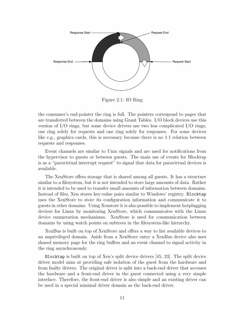
I/O rings have five components: the buffer itself and start- and end-pointersfor both the producer and consumer. The pointers are advanced when a re-quest/response is enqueued or completed. When the producer’s start-pointer reaches

10

Response Start Request End

Request StartResponse End

Figure 2.1: IO Ring

the consumer’s end-pointer the ring is full. The pointers correspond to pages thatare transferred between the domains using Grant Tables. I/O block devices use thisversion of I/O rings, but some device drivers use two less complicated I/O rings;one ring solely for requests and one ring solely for responses. For some deviceslike e.g., graphics cards, this is necessary because there is no 1:1 relation betweenrequests and responses.

Event channels are similar to Unix signals and are used for notifications fromthe hypervisor to guests or between guests. The main use of events for Blocktapis as a “paravirtual interrupt request” to signal that data for paravirtual devices isavailable.

The XenStore offers storage that is shared among all guests. It has a structuresimilar to a filesystem, but it is not intended to store large amounts of data. Ratherit is intended to be used to transfer small amounts of information between domains.Instead of files, Xen stores key-value pairs similar to Windows’ registry. Blocktapuses the XenStore to store its configuration information and communicate it toguests in other domains. Using Xenstore it is also possible to implement hotpluggingdevices for Linux by monitoring XenStore, which communicates with the Linuxdevice enumeration mechanisms. XenStore is used for communication betweendomains by using watch points on subtrees in the filesystem-like hierarchy.

XenBus is built on top of XenStore and offers a way to list available devices toan unprivileged domain. Aside from a XenStore entry a XenBus device also usesshared memory page for the ring buffers and an event channel to signal activity inthe ring asynchronously.

Blocktap is built on top of Xen’s split device drivers [45, 23]. The split devicedriver model aims at providing safe isolation of the guest from the hardware andfrom faulty drivers. The original driver is split into a back-end driver that accessesthe hardware and a front-end driver in the guest connected using a very simpleinterface. Therefore, the front-end driver is also simple and an existing driver canbe used in a special minimal driver domain as the back-end driver.

11

All of these data structures are used in the same way in Blocktap as in the splitdevice driver: data structures containing metadata about requests are enqueued inthe ring buffer and issued and responses are written to the same buffer. Data istransferred out-of-band using grant references, which makes fast DMA transferspossible [20]. Note that because of limited space in the I/O ring, the maximumrequest size is 44 KB [20].

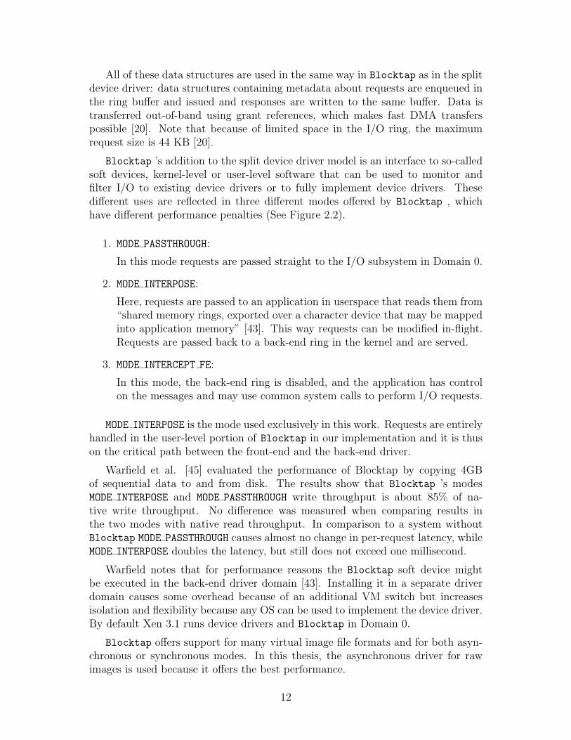
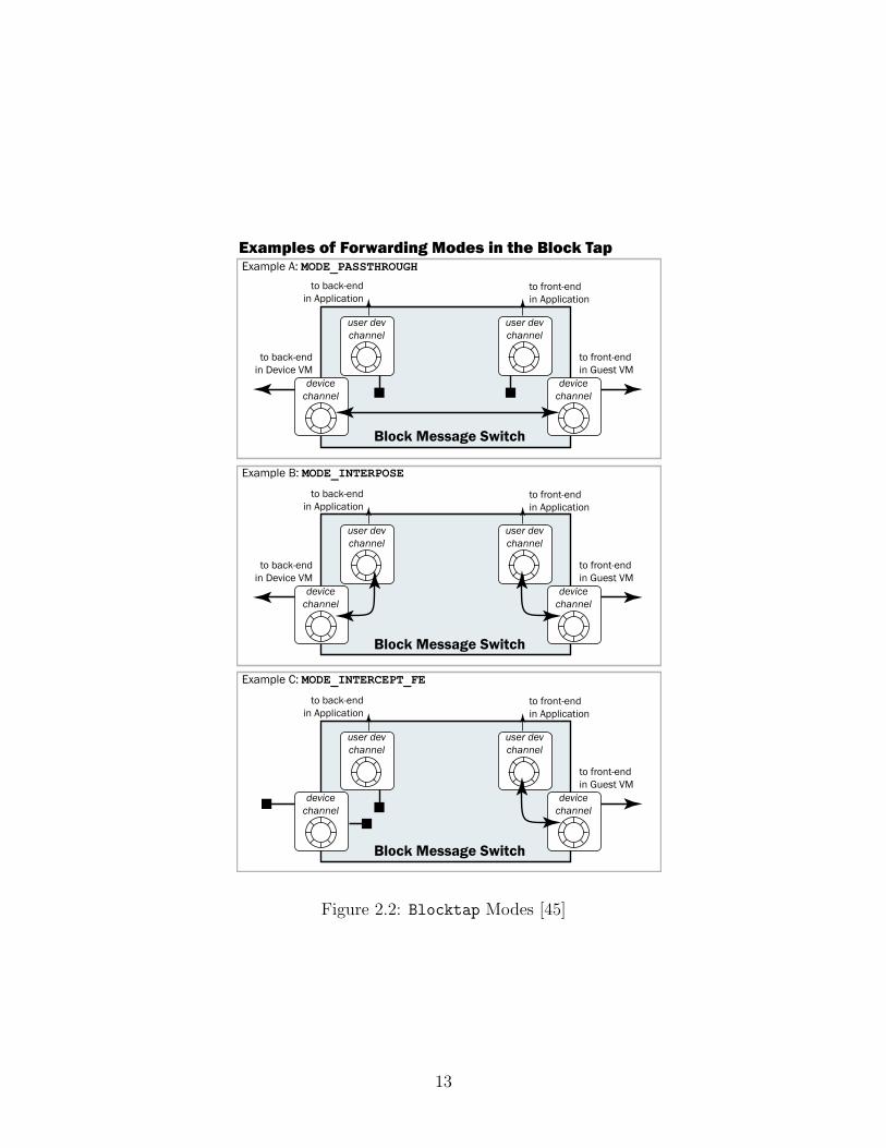
Blocktap ’s addition to the split device driver model is an interface to so-calledsoft devices, kernel-level or user-level software that can be used to monitor andfilter I/O to existing device drivers or to fully implement device drivers. Thesedifferent uses are reflected in three different modes offered by Blocktap , whichhave different performance penalties (See Figure 2.2).

1. MODE PASSTHROUGH:

In this mode requests are passed straight to the I/O subsystem in Domain 0.

2. MODE INTERPOSE:

Here, requests are passed to an application in userspace that reads them from“shared memory rings, exported over a character device that may be mappedinto application memory” [43]. This way requests can be modified in-flight.Requests are passed back to a back-end ring in the kernel and are served.

3. MODE INTERCEPT FE:

In this mode, the back-end ring is disabled, and the application has controlon the messages and may use common system calls to perform I/O requests.

MODE INTERPOSE is the mode used exclusively in this work. Requests are entirelyhandled in the user-level portion of Blocktap in our implementation and it is thuson the critical path between the front-end and the back-end driver.

Warfield et al. [45] evaluated the performance of Blocktap by copying 4GBof sequential data to and from disk. The results show that Blocktap ’s modesMODE INTERPOSE and MODE PASSTHROUGH write throughput is about 85% of na-tive write throughput. No difference was measured when comparing results inthe two modes with native read throughput. In comparison to a system withoutBlocktap MODE PASSTHROUGH causes almost no change in per-request latency, whileMODE INTERPOSE doubles the latency, but still does not exceed one millisecond.

Warfield notes that for performance reasons the Blocktap soft device mightbe executed in the back-end driver domain [43]. Installing it in a separate driverdomain causes some overhead because of an additional VM switch but increasesisolation and flexibility because any OS can be used to implement the device driver.By default Xen 3.1 runs device drivers and Blocktap in Domain 0.

Blocktap offers support for many virtual image file formats and for both asyn-chronous or synchronous modes. In this thesis, the asynchronous driver for rawimages is used because it offers the best performance.

12

Block Message Switch

devicechannel

devicechannel

user devchannel

user devchannel

Examples of Forwarding Modes in the Block Tap

to back-endin Device VM

to back-endin Application

to front-endin Guest VM

to front-endin Application

Example A: MODE_PASSTHROUGH


devicechannel

devicechannel

user devchannel

user devchannel

to back-endin Device VM




Example B: MODE_INTERPOSE


devicechannel

devicechannel

user devchannel

user devchannel




Example C: MODE_INTERCEPT_FE

Figure 3: Examples of forwarding modes.

bypass the user rings. Passthrough can be used to imple-ment kernel-level monitoring of block requests, or to im-plement soft devices in-kernel for improved performance.

MODE INTERPOSE routes all requests and replies acrossthe user rings. An application must attach to the block tapinterface and pass messages across the two rings, allow-ing complete monitoring and modification of the requeststream at the application level. This mode can be usedto modify in-flight requests, for instance to build a com-pressed or encrypted block store.

MODE INTERCEPT FE uses only the front-end rings onthe driver, disabling the back-end altogether. This mode al-lows the construction of full, application-level soft devices,using existing OS interfaces (such as memory, or mountedfile systems) as a backing store. This mode can be used toeasily prototype new functionality, or to forward block re-quests to a block device back-end on another physical host(after an OS migration, for instance1).

1OS migration is feature that we have recently added to Xen, allowinga running OS to move from one physical host to another while executing.One problem which managing migration is that local disks will be leftbehind.

3.2 The Application Interface

As shown in Figure 2, the user rings are exported to a char-acter device, which is mapped by a library allowing accessto the message rings and in-flight requests. Our currentimplementation allows chains of plugins to be attached tohandle block requests. We presently have plugins to pro-vide both copy-on-write and encrypted disks and to allowdirect access to image files and remote GNBD disks.

4 Evaluation

Figure 4 shows an analysis of the impact of soft devices onblock request performance with respect to both throughputand latency. Tests were performed on a Compaq ProliantDL360, which is a dual Pentium III 733MHz machine with72.8GB Ultra3 SCSI disks.

Throughput measurements aimed to test the maximumachievable read and write speeds to the local disk.The left graph in Figure 4 shows read and writethroughput moving four gigabytes of sequential data toand from disk. The three bars in the graph com-pare the throughput without using the block tap, usingthe block tap in MODE PASSTHROUGH, and finally inMODE INTERPOSE. As shown, our soft device interfaceresults in a minimal degradation of throughput. We are ca-pable of achieving 50MB/s read throughput, identical tothat achieved by Xen’s existing split drivers. On writes,we see about a 15% overhead; we are still investigating thesource of this loss of performance.

Latency measures the per-request overhead of synchronousrequests to disk. Given that disk requests are heavilybatched in general, this is a less meaningful measurementfor normal workloads. However, it does represent a worst-case overhead and also gives a clearer illustration of thecosts that our implementation imposes. The right graph inFigure 4 shows mean request times across 100,000 4-bytesynchronous writes. We see a small overhead in passingrequests through the kernel of the virtual device domainin MODE PASSTHROUGH, reflecting the cost of an addi-tional VM context switch and request/response copy2 ineach direction. MODE INTERPOSE is considerably moreexpensive as it adds two additional context switches andtwo message copies, in order to pass messages through auser-space application. There are additional costs in map-ping attached data pages to user space. However, even thisoverhead has insignificant impact given the length of av-erage disk seek times. We intend to explore the more de-manding performance requirements of network devices inthe coming months.

2Note that only the request and response structs (respectively 60 and7 bytes) are copied on the shared memory rings. Pages of data are refer-enced and mapped separately.

2005 USENIX Annual Technical Conference USENIX Association 381

Figure 2.2: Blocktap Modes [45]

13

Aside from the split device driver model, Blocktap has the following componentsin Domain 0 for devices:

character devices are used to communicate the issuance and completion of re-quests.

tapdisk is a user-level process, also called a tapdisk driver, that works with atleast one image file.

blktapctrl is a user-level daemon that controls the start and termination oftapdisk processes.

named pipes are used for communication between the tapdisk processes and theblktapctrl daemon for driver configuration and startup synchronization.

Meyer et al. [35] have redesigned Blocktap to use small reusable processingblocks to facilitate the development of soft devices. Instead of forcing the user tobuild his or her own user-level software device driver, they provide a set of reusableprocessing blocks that can be specified in a declarative language. This approachis also able to provide simple I/O request filtering, but no specific details of thepower of this language are given.

2.3 Data Stream Management System

Data stream management systems (DSMS) are a specialized type of database fordealing with streams of data. The problem of monitoring large amounts of datais well known. Monitoring financial data, e.g. stock market tickers, or detectingintrusions in a network system by monitoring all incoming network packets arepopular applications of DSMSs [13]. A data stream is a “real-time, continuous, or-dered (implicitly by arrival time or explicitly by timestamp) sequence of items”[25].Typically the size of the incoming data items is small, but the high arrival rate ofincoming items poses a challenging problem. Some of the requirements for a DSMSare listed by Golab et al. [25]: query semantics must allow time- and order-basedoperations, and no blocking operators that have to consume the whole input may beused. A side-effect of dynamic changes is that the database may encounter changesin the stream’s characteristics, e.g., its rate or burstiness.

Several projects have implemented DSMS prototypes. The most complete projectsavailable for academic purposes are STREAM [26] and Borealis [9]. Some technologyfrom the predecessor of Borealis, called Aurora, is used in a commercial productand is advertised as a monitoring solution for networks and financial stream data[40]. It is also used in surveillance and military operations. Another universityproject called PIPES follows a different idea [16]. Instead of offering a monolithicDSMS, it implements only a programming library that has to be customized fora particular use case. There are many other smaller projects: TelegraphCQ [18],

14

which uses a query language similar to that of PostgreSQL, the commercial kdb+database [29], and others. Further research has been done in StatStream [48] on thecomputation of statistics and could potentially be useful for efficient computationof statistic properties of single streams and pairs of streams. In particular, correla-tions can be computed very efficiently in StatStream using Fourier transformations[48].

2.3.1 DSMS Query Languages

Most DSMSs support a query language that is a subset of SQL and extend SQLwith windows. One notable exception is Borealis, which lets a user essentiallyspecify the exact physical operator plan. This way, query plan generation becomesmuch easier and no higher-level language has to be defined.

We are using the DSMS STREAM (STanford sTReam dAta Manager), that sup-ports queries expressed in CQL (Continuous Query Language) [12]. CQL supportssome basic commands from SQL and introduces a notion of streams in additionto static relations. STREAM [26] was developed at Stanford University. The projectwas officially wound down in 2006.

DSMSs usually keep stream data in memory to improve performance. How-ever, DSMS are more than in-memory database management systems. Because theamount of incoming data is unlimited, the data somehow have to be limited tofit in memory [25]. This is usually achieved by using summaries of data – calledsynopses – and by only considering sets of recent tuples. These sets are calledwindows and are usually defined by a tuple count limit or by a time interval. Ad-ditionally, some DSMSs allow the user to specify when an update of an observedwindow is produced. Windows in DSMSs are often specified as sliding windows.Here, all tuples in a recent time interval are included in the window on the stream.For example a window of 30 seconds includes all tuples that arrived in the last 30seconds. Similarly one can define a window over the last 30 requests.

Tumbling windows are different in that they never overlap with previous win-dows. In a 30 second tumbling window, after 30 seconds one window is reportedand after 60 seconds the second window is reported. Every 30 seconds a new non-overlapping window is reported.

2.3.2 DSMS Optimization/Plan Generation

All DSMSs have the problem in common that the optimization process should bedynamic, to account for fluctuating incoming streams. In a conventional relationalDBMS, the number of tuples in relations involved in a query might be measured,indexed, sampled, or estimated before executing the query, while this is impossiblefor a stream. Input rates might be measured and estimated but only after the queryhas begun execution. Therefore, a query plan should be dynamic and able to reactto increasing or decreasing input rates.

15

STREAM does optimizations to reduce the memory consumption when process-ing streams [13] but does not perform dynamic optimization of query plans. ForBorealis [11] dynamic query plan optimization can be performed using a plainload-balancing scheme or a scheme that is based on the correlation between streams[47]. These schemes aim to evenly balance the load on all machines in contrast toour goal of reducing the load on the server nodes.

Cheung and Madden [19] have done work in the area of DSMS, that addressesproblems similar to the ones we tackle in our work. They monitor the executionof user applications by activating certain probes in an application’s code. Thisis very similar to DTrace’s and VProbes’ aquisitional framework. The informa-tion gathered from these probes includes function invocations, variable values andmemory usage. Any such information is forwarded to a DSMS that performs queryprocessing, in much the same way as we use STREAM to process queries over I/Oevent records. For distributing the processing on several servers they have devisedoptimizations to reduce the load on the server nodes. Part of the processing of theDSMS is executed on the server nodes and some is performed on other nodes. Theyhave considered the trade-off between CPU utilization on the server node and thenetwork’s bandwidth.

In general it is more favourable to keep the CPU utilization on the server nodeas low as possible so as to not interfere with applications that are being monitored,but when network bandwidth is scarce it might be better to perform more filtering.We use the same rationale for optimizations in our approach.

The main differences between this work and the approach by Cheung and Mad-den, called EndoScope [19], is the different application domain, which also resultsin a very different optimization goal. EndoScope instruments an application withprobes and thus the focus of optimization is to determine the probes that incurthe least performance impact. In our work only one continuous data source at onefixed location is considered.

16

Chapter 3

System Design

3.1 System Organization

In this thesis we present a system for monitoring storage I/O activity in virtualmachines. The monitored statistics can be customized using a flexible query lan-guage. The data stream management system STREAM processes the logged dataon I/O requests by executing the user’s queries. The DSMS is distributed on theserver nodes that host the virtual machines and a central monitoring node.

Figure 3.1 illustrates our architecture. We monitor the storage I/O to and fromvirtual machines hosted on server nodes. Each of these server nodes hosts severalvirtual machines that are backed by image files on local hard disks. In each of theserver nodes an instance of a DSMS is running in Domain 0. Another DSMS isrunning on a central monitoring node that is receiving packets over the networkfrom the DSMS instances on the server nodes. We call a DSMS instance on a servernode a “filter” DSMS, because this instance mainly filters selected tuples from themonitored data. Conversely, the DSMS receiving tuples on the monitoring node iscalled the “monitor” DSMS. It performs any remaining processing on the tuples.

Inside the server nodes, the filter instances receive the data about I/O requestsfrom an extension to the normal mechanism that virtualizes disk I/O in Xen. Ontop of serving the I/O requests, it logs the properties of requests to a Unix domainsocket, which is read by the filter DSMS.

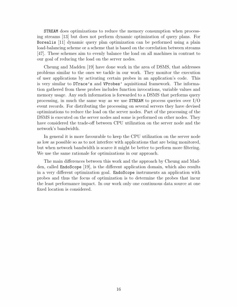
In order to explain the different components of our system, we look at whatevents occur in the virtual machines, the server’s Domain 0, and the monitoringnode. The active components of our system in the virtual machine – or user domainas opposed to Domain 0 – are described in Figure 3.2. The terms user domain andDomain 0 are abbreviated to DomU and Dom0. Any workload that performs I/Ooperations in the virtual machines can access several underlying virtual disks. Inthe example there is a virtual root partition /dev/sda1 and a virtual swap partition.In the virtual machine’s Linux kernel all of the requests are sent to a frontend driver(Xen blkfront) and are ultimately performed by a backend (Xen Blocktap ) inDomain 0. The interface in Domain 0’s kernel is called blktap.

17

Monitor Node

Server Node Server Node Server Node

+

Queries Results

+*Filter DSMSMonitor DSMS

Disk Disk Disk

Unix domain socket

UDP socket

** *

VM VM VM VM VMVM

Figure 3.1: I/O Monitoring Architecture

Xen blktap

Dom0Kernel

Xen blkfront

Xen blkfront

Req/Resp

Req/Resp

Workload

Req/Resp

Req/Resp

Virtual Diskswap

Virtual Disksda1

DomUKernelDomU Userspace

Req/Resp

Req/Resp

Figure 3.2: Guest Domain

18

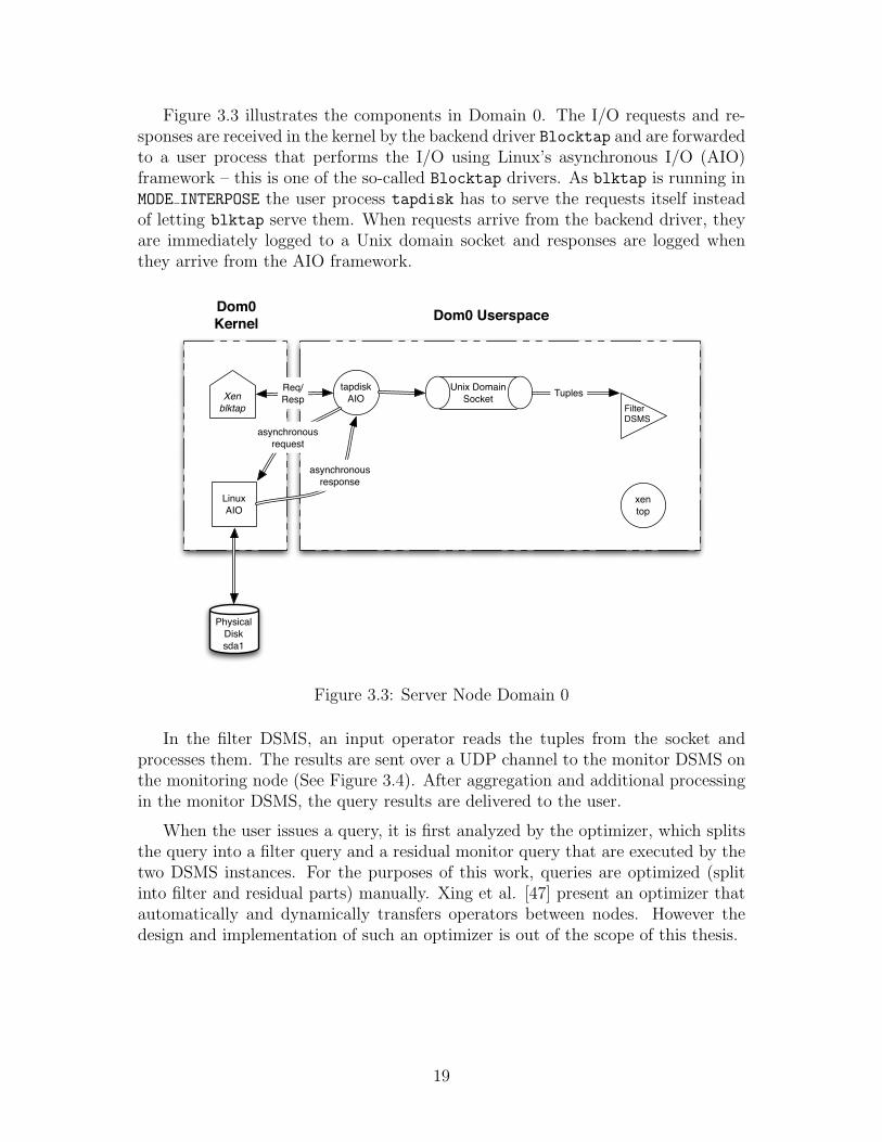
Figure 3.3 illustrates the components in Domain 0. The I/O requests and re-sponses are received in the kernel by the backend driver Blocktap and are forwardedto a user process that performs the I/O using Linux’s asynchronous I/O (AIO)framework – this is one of the so-called Blocktap drivers. As blktap is running inMODE INTERPOSE the user process tapdisk has to serve the requests itself insteadof letting blktap serve them. When requests arrive from the backend driver, theyare immediately logged to a Unix domain socket and responses are logged whenthey arrive from the AIO framework.

Unix DomainSocket Tuplestapdisk

AIO

Dom0 Userspace

Physical Disksda1

Linux AIO

Req/Resp

xentop

Xen blktap

Dom0Kernel

asynchronous request

asynchronousresponse

FilterDSMS

Figure 3.3: Server Node Domain 0

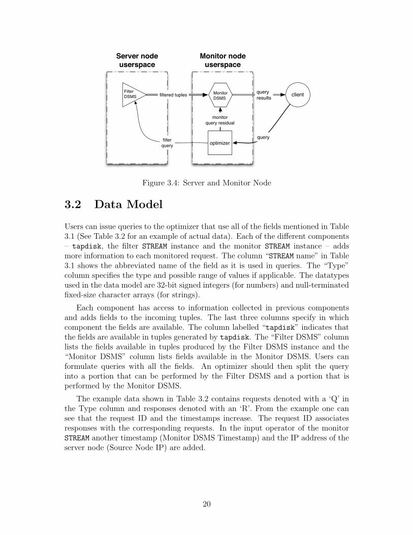
In the filter DSMS, an input operator reads the tuples from the socket andprocesses them. The results are sent over a UDP channel to the monitor DSMS onthe monitoring node (See Figure 3.4). After aggregation and additional processingin the monitor DSMS, the query results are delivered to the user.

When the user issues a query, it is first analyzed by the optimizer, which splitsthe query into a filter query and a residual monitor query that are executed by thetwo DSMS instances. For the purposes of this work, queries are optimized (splitinto filter and residual parts) manually. Xing et al. [47] present an optimizer thatautomatically and dynamically transfers operators between nodes. However thedesign and implementation of such an optimizer is out of the scope of this thesis.

19

optimizer

monitor query residual

query

queryresults

Monitor nodeuserspace

Server nodeuserspace

filterquery

filtered tuples clientFilterDSMS

MonitorDSMS

Figure 3.4: Server and Monitor Node

3.2 Data Model

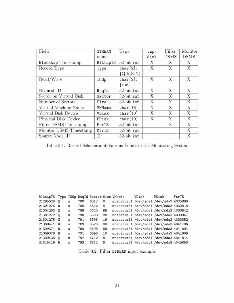
Users can issue queries to the optimizer that use all of the fields mentioned in Table3.1 (See Table 3.2 for an example of actual data). Each of the different components– tapdisk, the filter STREAM instance and the monitor STREAM instance – addsmore information to each monitored request. The column “STREAM name” in Table3.1 shows the abbreviated name of the field as it is used in queries. The “Type”column specifies the type and possible range of values if applicable. The datatypesused in the data model are 32-bit signed integers (for numbers) and null-terminatedfixed-size character arrays (for strings).

Each component has access to information collected in previous componentsand adds fields to the incoming tuples. The last three columns specify in whichcomponent the fields are available. The column labelled “tapdisk” indicates thatthe fields are available in tuples generated by tapdisk. The “Filter DSMS” columnlists the fields available in tuples produced by the Filter DSMS instance and the“Monitor DSMS” column lists fields available in the Monitor DSMS. Users canformulate queries with all the fields. An optimizer should then split the queryinto a portion that can be performed by the Filter DSMS and a portion that isperformed by the Monitor DSMS.

The example data shown in Table 3.2 contains requests denoted with a ‘Q’ inthe Type column and responses denoted with an ‘R’. From the example one cansee that the request ID and the timestamps increase. The request ID associatesresponses with the corresponding requests. In the input operator of the monitorSTREAM another timestamp (Monitor DSMS Timestamp) and the IP address of theserver node (Source Node IP) are added.

20

Field STREAM

nameType tap-

disk

FilterDSMS

MonitorDSMS

Blocktap Timestamp BlktapTS 32-bit int X X XRecord Type Type char[2]:

{Q,R,E,N}X X X

Read/Write IOOp char[2]:{r,w}

X X X

Request ID ReqId 32-bit int X X XSector on Virtual Disk Sector 32-bit int X X XNumber of Sectors Size 32-bit int X X XVirtual Machine Name VMName char[15] X X XVirtual Disk Device VDisk char[10] X X XPhysical Disk Device PDisk char[10] X X XFilter DSMS Timestamp FtrTS 32-bit int X XMonitor DSMS Timestamp MtrTS 32-bit int XSource Node IP IP 32-bit int X

Table 3.1: Record Schemata at Various Points in the Monitoring System

BlktapTS Type IOOp ReqId Sector Size VMName VDisk PDisk FtrTS21295029 Q w 788 6512 8 muscatvm51 /dev/sda1 /dev/sda3 402589021301076 R w 788 6512 8 muscatvm51 /dev/sda1 /dev/sda3 403381821301263 Q w 789 6520 88 muscatvm51 /dev/sda1 /dev/sda3 403384221301272 Q w 790 6608 88 muscatvm51 /dev/sda1 /dev/sda3 403384721301278 Q w 791 6696 16 muscatvm51 /dev/sda1 /dev/sda3 403385221308471 R w 789 6520 88 muscatvm51 /dev/sda1 /dev/sda3 404179621309371 R w 790 6608 88 muscatvm51 /dev/sda1 /dev/sda3 404180421309378 R w 791 6696 16 muscatvm51 /dev/sda1 /dev/sda3 404180921309438 Q w 792 6712 8 muscatvm51 /dev/sda1 /dev/sda3 404181421315419 R w 792 6712 8 muscatvm51 /dev/sda1 /dev/sda3 4045853

Table 3.2: Filter STREAM input example

21

3.2.1 Timestamps

Timestamps are collected at three logical components of the system:

1. At the tapdisk process, when the request is first queued and when it hasbeen completed (BlktapTS).

2. In the input operator of the Filter STREAM instance on the server node (FtrTS).

3. In the input operator of the Monitor STREAM instance on the monitor node(MtrTS).

The BlktapTS records the times when a request is actually queued and com-pleted. For technical reasons two other timestamps have to be recorded for STREAM.

STREAM internally uses timestamps, e.g., to calculate when a tuple is not con-tained in a time-based window anymore. STREAM requires tuples to arrive in non-decreasing timestamp order. Our monitoring system consists of several differentprocesses running on several physical machines. In this setting it would be difficultto guarantee perfect synchronization of clocks. Scheduling of different processes andnetwork congestion can modify the order the requests arrive in the DSMS. This is acommon problem in distributed DSMSs. STREAM does not address this problem andtreats out-of-order timestamps as fatal errors. An acceptable work-around to thisproblem would be to ensure synchronized clocks with another technique such as thenetwork time protocol (NTP) at regular intervals. Then the maximum differencein the clocks of the different virtual and physical machines could be specified. TheDSMS should then regard tuples arriving at different timestamps within the inter-val specified by this imprecision as arriving at the same time instant. To accomplishthis with STREAM , one would have to implement a notion of imprecision in all ofSTREAM’s operators, but this modification is out of the scope of this work. In oursimple work-around to this general problem, each STREAM instance collects a newtimestamp for a tuple when it is read in STREAM’s input filter. Thus the timestampwill never decrease.

Originally, timestamps in STREAM are measured in seconds, but disk access times,seek times and rotational latency are usually on the order of milliseconds. Microsec-ond granularity has been chosen for this work because it allows us to capture theseI/O related durations.

Timestamps are stored using signed 32-bit integers. Ideally, timestamps wouldbe recorded as unsigned 64-bit integers but this datatype is not supported bySTREAM. Adding this datatype would have required significant changes to STREAM’s

parser and operators. Instead we use the built-in 32-bit integer type. Due to thisvery limited size of timestamps we do not use timestamps relative to the Unixepoch. When we consider a granularity of microseconds, signed 32-bit integers canonly cover time periods of up to 35 minutes. Therefore the three timestamps referto the start of the respective component as a point of reference. For a more realis-tic scenario the problem of clock synchronization should be addressed and a more

22

flexible datatype for timestamps should be added to STREAM. These changes are outof the scope of this work.

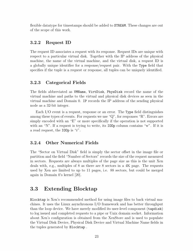
3.2.2 Request ID

The request ID associates a request with its response. Request IDs are unique withrespect to a particular virtual disk. Together with the IP address of the physicalmachine, the name of the virtual machine, and the virtual disk, a request ID isa globally unique identifier for a response/request pair. With the Type field thatspecifies if the tuple is a request or response, all tuples can be uniquely identified.

3.2.3 Categorical Fields

The fields abbreviated as VMName, VirtDisk, PhysDisk record the name of thevirtual machine and paths to the virtual and physical disk devices as seen in thevirtual machine and Domain 0. IP records the IP address of the sending physicalnode as a 32-bit integer.

Each I/O event is a request, response or an error. The Type field distinguishesamong these types of events. For requests we use “Q”, for responses “R”. Errors aresimply encoded with an “E” or more specifically if the operation is not supportedwith an “N”. If a request is trying to write, its IOOp column contains “w”. If it isa read request, the IOOp is “r”.

3.2.4 Other Numerical Fields

The “Sector on Virtual Disk” field is simply the sector offset in the image file orpartition and the field “Number of Sectors” records the size of the request measuredin sectors. Requests are always multiples of the page size as this is the unit Xendeals with, e.g., multiples of 8 as there are 8 sectors in a 4K page. The requestsused by Xen are limited to up to 11 pages, i.e. 88 sectors, but could be mergedagain in Domain 0’s kernel [20].

3.3 Extending Blocktap

Blocktap is Xen’s recommended method for using image files to back virtual ma-chines. It uses the Linux asynchronous I/O framework and has better throughputthan the loop device. We have merely modified its user-level component (tapdisk)to log issued and completed requests to a pipe or Unix domain socket. Informationabout Xen’s configuration is obtained from the XenStore and is used to populatethe Virtual Disk Device, Physical Disk Device and Virtual Machine Name fields inthe tuples generated by Blocktap .

23

3.4 Extending STREAM

STREAM is modified mainly in two areas: input and output operators and operatorscheduling. The last released version of STREAM (0.6.0) features a command lineinterface and a Java GUI client. Both assume that input tuples are read from a filein a CSV-like file format. Each tuple in this file defines a tuple in an input stream.One has to specify the timestamp at which the tuple can be read by STREAM atthe granularity of seconds. To measure significant numbers for I/O requests thisgranularity was changed to microseconds, which allows a maximum of 35 minutes ofexperiment runtime (See Section 3.2.1). Instead of using the script input operator,an input operator for UDP sockets was added.

In order to measure STREAM’s performance we are comparing the CPU uti-lization of different CQL queries, but STREAM is using a scheduler that essentiallybusy-waits on all the operators. When an operator is scheduled it processes a fixednumber of tuples before returning control to the scheduler. If operators have noinput to process, they simply return immediately to the scheduler, which handscontrol to another operator. If STREAM has no tuples to process, it effectively con-tinuously polls for new tuples. The effect of this is that STREAM always fully utilizesone processor of the computer. We have changed this by simply adding a sleep callfor the STREAM thread of 100 microseconds in case none of the operators have anytuples to process. As a result, STREAM will have higher CPU utilization when it hasmore tuples to process or more work per tuple, and we can use measurements ofCPU utilization to quantify the costs of monitoring I/O activity. We have imple-mented this simple approach, but an alternate solution would be to use the poll

system call in the input operator to find out when there is new data to process.

3.5 Monitoring Queries

To demonstrate the capabilities of our monitoring system we list some examplequeries. Some of the queries were chosen to show the greater flexibility of ourapproach compared with such tools as iostat while others show how differentqueries affect the performance differently. A subset of the queries is explainedbelow. The remaining queries that are used in the experiments are shown in theAppendix.

The queries are expressed in CQL. The semantics of CQL are described in theSTREAM manual [6], the CQL grammar specification [2] and the technical report onthe design of CQL [12]. For each query we provide a sample of the beginning of theinput to STREAM and the corresponding output according to the query. The inputstream from Blocktap is called IOstream and the names of the different fieldsare listed in Table 3.1. Sample input and output were given for a filter STREAM

instance that reads tuples directly from Blocktap . The data presented is from anexperiment as defined in Chapter 4.

24

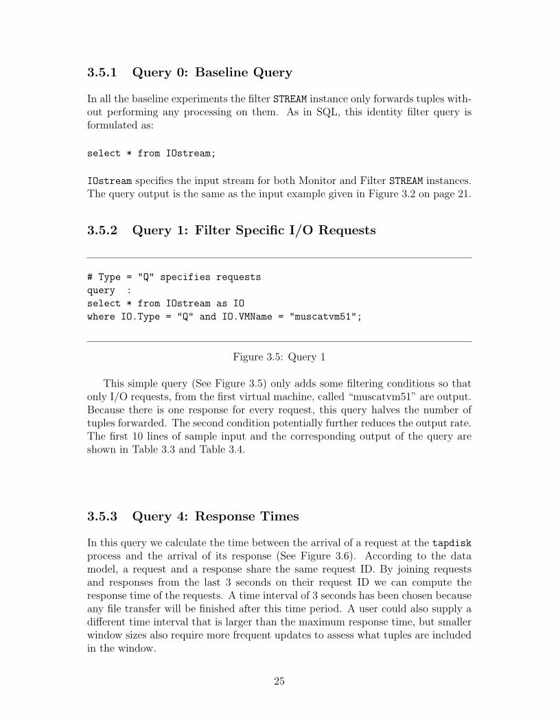
3.5.1 Query 0: Baseline Query

In all the baseline experiments the filter STREAM instance only forwards tuples with-out performing any processing on them. As in SQL, this identity filter query isformulated as:

select * from IOstream;

IOstream specifies the input stream for both Monitor and Filter STREAM instances.The query output is the same as the input example given in Figure 3.2 on page 21.

3.5.2 Query 1: Filter Specific I/O Requests

# Type = "Q" specifies requests

query :

select * from IOstream as IO

where IO.Type = "Q" and IO.VMName = "muscatvm51";

Figure 3.5: Query 1

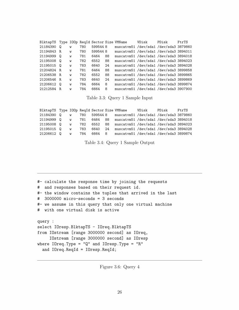
This simple query (See Figure 3.5) only adds some filtering conditions so thatonly I/O requests, from the first virtual machine, called “muscatvm51” are output.Because there is one response for every request, this query halves the number oftuples forwarded. The second condition potentially further reduces the output rate.The first 10 lines of sample input and the corresponding output of the query areshown in Table 3.3 and Table 3.4.

3.5.3 Query 4: Response Times

In this query we calculate the time between the arrival of a request at the tapdisk

process and the arrival of its response (See Figure 3.6). According to the datamodel, a request and a response share the same request ID. By joining requestsand responses from the last 3 seconds on their request ID we can compute theresponse time of the requests. A time interval of 3 seconds has been chosen becauseany file transfer will be finished after this time period. A user could also supply adifferent time interval that is larger than the maximum response time, but smallerwindow sizes also require more frequent updates to assess what tuples are includedin the window.

25


Table 3.3: Query 1 Sample Input

BlktapTS Type IOOp ReqId Sector Size VMName VDisk PDisk FtrTS21184390 Q w 780 599544 8 muscatvm51 /dev/sda1 /dev/sda3 387986021194999 Q w 781 6464 88 muscatvm51 /dev/sda1 /dev/sda3 389401821195008 Q w 782 6552 88 muscatvm51 /dev/sda1 /dev/sda3 389402321195015 Q w 783 6640 24 muscatvm51 /dev/sda1 /dev/sda3 389402821206612 Q w 784 6664 8 muscatvm51 /dev/sda1 /dev/sda3 3899874

Table 3.4: Query 1 Sample Output

#- calculate the response time by joining the requests

# and responses based on their request id.

#- the window contains the tuples that arrived in the last

# 3000000 micro-seconds = 3 seconds

#- we assume in this query that only one virtual machine

# with one virtual disk is active

query :

select IOresp.BlktapTS - IOreq.BlktapTS

from IOstream [range 3000000 second] as IOreq,

IOstream [range 3000000 second] as IOresp

where IOreq.Type = "Q" and IOresp.Type = "R"

and IOreq.ReqId = IOresp.ReqId;

Figure 3.6: Query 4

26

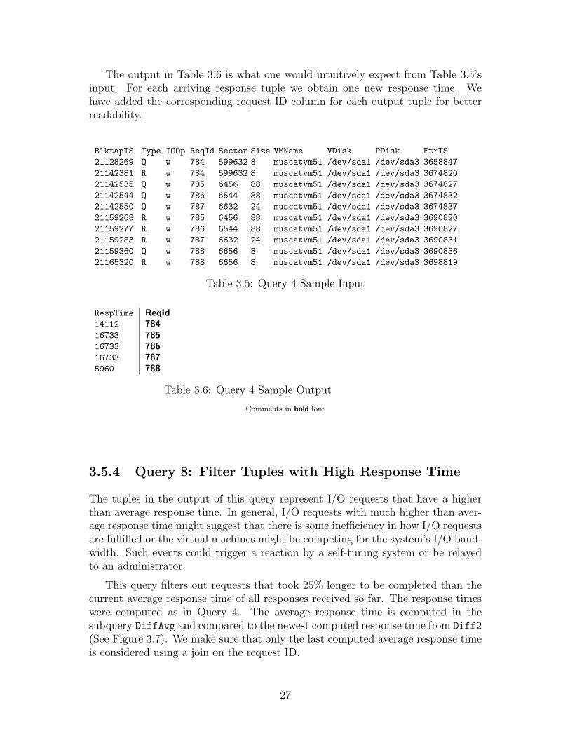
The output in Table 3.6 is what one would intuitively expect from Table 3.5’sinput. For each arriving response tuple we obtain one new response time. Wehave added the corresponding request ID column for each output tuple for betterreadability.



RespTime ReqId14112 78416733 78516733 78616733 7875960 788


Comments in bold font

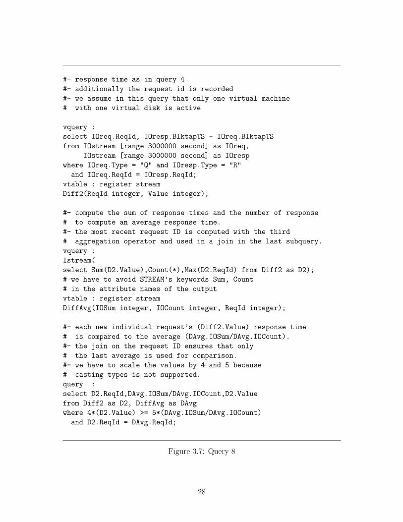
3.5.4 Query 8: Filter Tuples with High Response Time

The tuples in the output of this query represent I/O requests that have a higherthan average response time. In general, I/O requests with much higher than aver-age response time might suggest that there is some inefficiency in how I/O requestsare fulfilled or the virtual machines might be competing for the system’s I/O band-width. Such events could trigger a reaction by a self-tuning system or be relayedto an administrator.

This query filters out requests that took 25% longer to be completed than thecurrent average response time of all responses received so far. The response timeswere computed as in Query 4. The average response time is computed in thesubquery DiffAvg and compared to the newest computed response time from Diff2

(See Figure 3.7). We make sure that only the last computed average response timeis considered using a join on the request ID.

27

#- response time as in query 4

#- additionally the request id is recorded



vquery :

select IOreq.ReqId, IOresp.BlktapTS - IOreq.BlktapTS




and IOreq.ReqId = IOresp.ReqId;

vtable : register stream

Diff2(ReqId integer, Value integer);

#- compute the sum of response times and the number of response

# to compute an average response time.

#- the most recent request ID is computed with the third

# aggregation operator and used in a join in the last subquery.

vquery :

Istream(

select Sum(D2.Value),Count(*),Max(D2.ReqId) from Diff2 as D2);

# we have to avoid STREAM’s keywords Sum, Count

# in the attribute names of the output


DiffAvg(IOSum integer, IOCount integer, ReqId integer);

#- each new individual request’s (Diff2.Value) response time

# is compared to the average (DAvg.IOSum/DAvg.IOCount).

#- the join on the request ID ensures that only

# the last average is used for comparison.

#- we have to scale the values by 4 and 5 because

# casting types is not supported.

query :

select D2.ReqId,DAvg.IOSum/DAvg.IOCount,D2.Value

from Diff2 as D2, DiffAvg as DAvg

where 4*(D2.Value) >= 5*(DAvg.IOSum/DAvg.IOCount)

and D2.ReqId = DAvg.ReqId;

Figure 3.7: Query 8

28

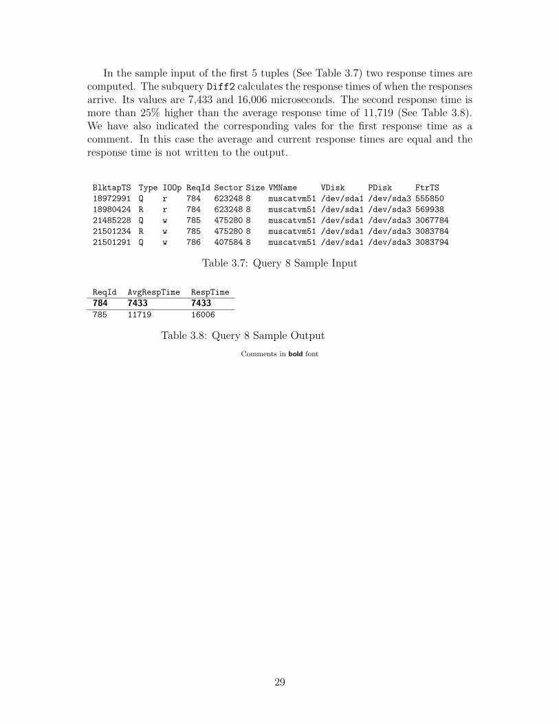
In the sample input of the first 5 tuples (See Table 3.7) two response times arecomputed. The subquery Diff2 calculates the response times of when the responsesarrive. Its values are 7,433 and 16,006 microseconds. The second response time ismore than 25% higher than the average response time of 11,719 (See Table 3.8).We have also indicated the corresponding vales for the first response time as acomment. In this case the average and current response times are equal and theresponse time is not written to the output.

BlktapTS Type IOOp ReqId Sector Size VMName VDisk PDisk FtrTS18972991 Q r 784 623248 8 muscatvm51 /dev/sda1 /dev/sda3 55585018980424 R r 784 623248 8 muscatvm51 /dev/sda1 /dev/sda3 56993821485228 Q w 785 475280 8 muscatvm51 /dev/sda1 /dev/sda3 306778421501234 R w 785 475280 8 muscatvm51 /dev/sda1 /dev/sda3 308378421501291 Q w 786 407584 8 muscatvm51 /dev/sda1 /dev/sda3 3083794


ReqId AvgRespTime RespTime784 7433 7433785 11719 16006


Comments in bold font

29

Chapter 4

Experimental Results

4.1 Overview of Experiments

We have conducted a series of experiments to show how the system performs incomparison to a baseline and how different circumstances modify these results. Inparticular we answer the following questions:

1. What is the overhead of collecting I/O event tuples?

2. How does the overhead vary with the complexity of the query?

3. How does the performance scale with the number of concurrently executedqueries?

4. Can we reduce the performance impact on the server node by offloading pro-cessing to the monitor node?

5. Does filtering of requests at the server node reduce load on the monitor node?

6. How does the system scale with the number of server nodes and virtual ma-chines?

4.2 Experimental Testbed

The equipment used for the experiments is an IBM Blade Center. The BladeCenter has a Model H chassis containing 28 blades, model number LS-21. Fromthese we used four of the blades, with up to three as the server node and one as themonitoring node. The blades used have two AMD dual-core 2212 HE CPUs at 2.0GHz, 10GB of RAM, and a single 67GB 10000 RPM internal hard disk. The disk’svendor is Fujitsu and the model used is a MBB2073RC. The virtual machines arebacked by image files on this local hard disk. The nodes are connected over aninternal network with 1Gb of bandwidth.

30

The operating system installed on the machines is OpenSuSE 10.3 with the dis-tribution package of Xen, which is in version 3.1. The source code of the user-levelprocesses providing Blocktap functionality is modified for some of the experiments.In all experiments the Linux kernel version 2.6.22 is used. The experiment drivernode is another computer that only executes a script that starts and stops compo-nents and evaluates their output.

4.2.1 Virtual Machine Configuration

In our experiments we use paravirtualized guest domains. The guest domains rundebian 4.0 Linux in a very minimal version. The guest domains use the sameLinux kernel 2.6.22 with Xen modifications as Domain 0. Each virtual machine hasone ext3 filesystem backed by an image file as root partition of size 4.8GB. Theroot partition uses the Blocktap backend driver. No swap partition is used in theexperiments. The root partition image is stored on a 19GB ext3 partition on theinternal hard disk. Each of the virtual machines uses a fixed 256MB of the servernode’s 10GB of RAM. Domain 0 uses all of the remaining RAM not used by guestdomains.

Each virtual machine is assigned a different processor core. Use of a prede-termined core for each virtual machine guarantees that we are not liable to anyunfairness in CPU scheduling, that could slow down one virtual machine in favourof another.

4.2.2 Measurement Tools

In the experiments xentop is used to measure CPU utilization in Domain 0 andin the guest domains. Version 3.1 of xentop is patched to flush its output to diskwhen terminated.

xentop reports one utilization value and does not differentiate between systemor user time and scales all results to the number of virtual cpus allocated to avirtual machine. For a virtual machine with four virtual CPUs, xentop reports anumber from 0 to 400. With four virtual CPUs of which one is fully utilized, xentopreports 100% utilization. In the experiments each guest domain and Domain 0 areassigned one VCPU. Thus the maximum utilization for measurements is 100%.

4.2.3 Experiment Methodology

Figure 4.1 illustrates how the experiments are set up. The experiment driver run-ning on the experiment node runs the experiments in five steps:

1. The monitor DSMS instance is started, if the experiment requires it.

31

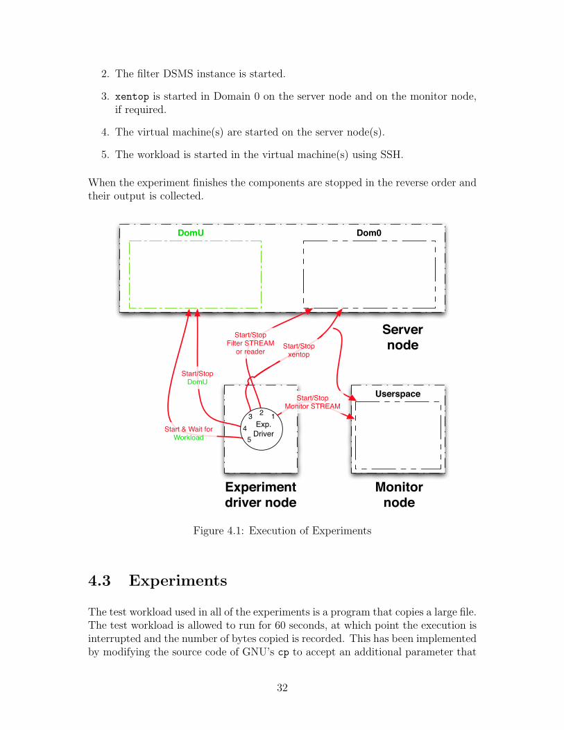
2. The filter DSMS instance is started.

3. xentop is started in Domain 0 on the server node and on the monitor node,if required.

4. The virtual machine(s) are started on the server node(s).

5. The workload is started in the virtual machine(s) using SSH.

When the experiment finishes the components are stopped in the reverse order andtheir output is collected.

DomU Dom0

Userspace

Start/Stop DomU

Start/Stopxentop

Start/StopMonitor STREAM

Start & Wait for Workload

Experiment driver node

Monitornode

Start/StopFilter STREAM

or reader

Servernode

Exp. Driver

123

54

Figure 4.1: Execution of Experiments

4.3 Experiments

The test workload used in all of the experiments is a program that copies a large file.The test workload is allowed to run for 60 seconds, at which point the execution isinterrupted and the number of bytes copied is recorded. This has been implementedby modifying the source code of GNU’s cp to accept an additional parameter that

32

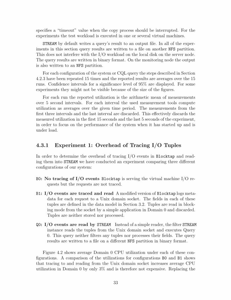
specifies a “timeout” value when the copy process should be interrupted. For theexperiments the test workload is executed in one or several virtual machines.

STREAM by default writes a query’s result to an output file. In all of the exper-iments in this section query results are written to a file on another NFS partition.This does not interfere with the I/O workload on the local disk on the server node.The query results are written in binary format. On the monitoring node the outputis also written to an NFS partition.

For each configuration of the system or CQL query the steps described in Section4.2.3 have been repeated 15 times and the reported results are averages over the 15runs. Confidence intervals for a significance level of 95% are displayed. For someexperiments they might not be visible because of the size of the figures.

For each run the reported utilization is the arithmetic mean of measurementsover 5 second intervals. For each interval the used measurement tools computeutilization as averages over the given time period. The measurements from thefirst three intervals and the last interval are discarded. This effectively discards themeasured utilization in the first 15 seconds and the last 5 seconds of the experiment,in order to focus on the performance of the system when it has started up and isunder load.

4.3.1 Experiment 1: Overhead of Tracing I/O Tuples

In order to determine the overhead of tracing I/O events in Blocktap and read-ing them into STREAM we have conducted an experiment comparing three differentconfigurations of our system:

B0: No tracing of I/O events Blocktap is serving the virtual machine I/O re-quests but the requests are not traced.

B1: I/O events are traced and read A modified version of Blocktap logs meta-data for each request to a Unix domain socket. The fields in each of thesetuples are defined in the data model in Section 3.2. Tuples are read in block-ing mode from the socket by a simple application in Domain 0 and discarded.Tuples are neither stored nor processed.

Q0: I/O events are read by STREAM Instead of a simple reader, the filter STREAMinstance reads the tuples from the Unix domain socket and executes Query0. This query neither filters any tuples nor processes their fields. The queryresults are written to a file on a different NFS partition in binary format.

Figure 4.2 shows average Domain 0 CPU utilization under each of these con-figurations. A comparison of the utilizations for configurations B0 and B1 showsthat tracing to and reading from the Unix domain socket increases average CPUutilization in Domain 0 by only 3% and is therefore not expensive. Replacing the

33

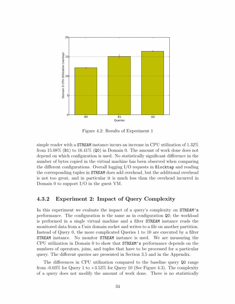
B0 B1 Q0Queries

0

5

10

15

20

Dom

ain

0 C

PU

Uti

lizati

on (

xento

p)

Figure 4.2: Results of Experiment 1

simple reader with a STREAM instance incurs an increase in CPU utilization of 1.32%from 15.08% (B1) to 16.41% (Q0) in Domain 0. The amount of work done does notdepend on which configuration is used. No statistically significant difference in thenumber of bytes copied in the virtual machine has been observed when comparingthe different configurations. Overall logging I/O requests in Blocktap and readingthe corresponding tuples in STREAM does add overhead, but the additional overheadis not too great, and in particular it is much less than the overhead incurred inDomain 0 to support I/O in the guest VM.

4.3.2 Experiment 2: Impact of Query Complexity

In this experiment we evaluate the impact of a query’s complexity on STREAM’s

performance. The configuration is the same as in configuration Q0; the workloadis performed in a single virtual machine and a filter STREAM instance reads themonitored data from a Unix domain socket and writes to a file on another partition.Instead of Query 0, the more complicated Queries 1 to 10 are executed by a filterSTREAM instance. No monitor STREAM instance is used. We are measuring theCPU utilization in Domain 0 to show that STREAM’s performance depends on thenumbers of operators, joins, and tuples that have to be processed for a particularquery. The different queries are presented in Section 3.5 and in the Appendix.

The differences in CPU utilization compared to the baseline query Q0 rangefrom -0.03% for Query 1 to +3.53% for Query 10 (See Figure 4.3). The complexityof a query does not modify the amount of work done. There is no statistically

34

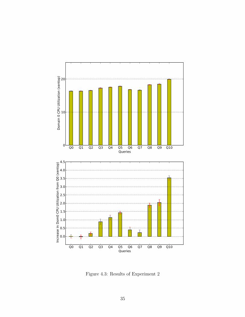
Q0 Q1 Q2 Q3 Q4 Q5 Q6 Q7 Q8 Q9 Q10Queries

0

10

20

Dom

ain

0 C

PU

Uti

lizati

on (

xento

p)

Q0 Q1 Q2 Q3 Q4 Q5 Q6 Q7 Q8 Q9 Q10Queries

0.0

0.5

1.0

1.5

2.0

2.5

3.0

3.5

4.0

4.5

Incr

ease

in D

om

0 C

PU

Uti

lizati

on f

rom

Q0 (

xento

p)


35

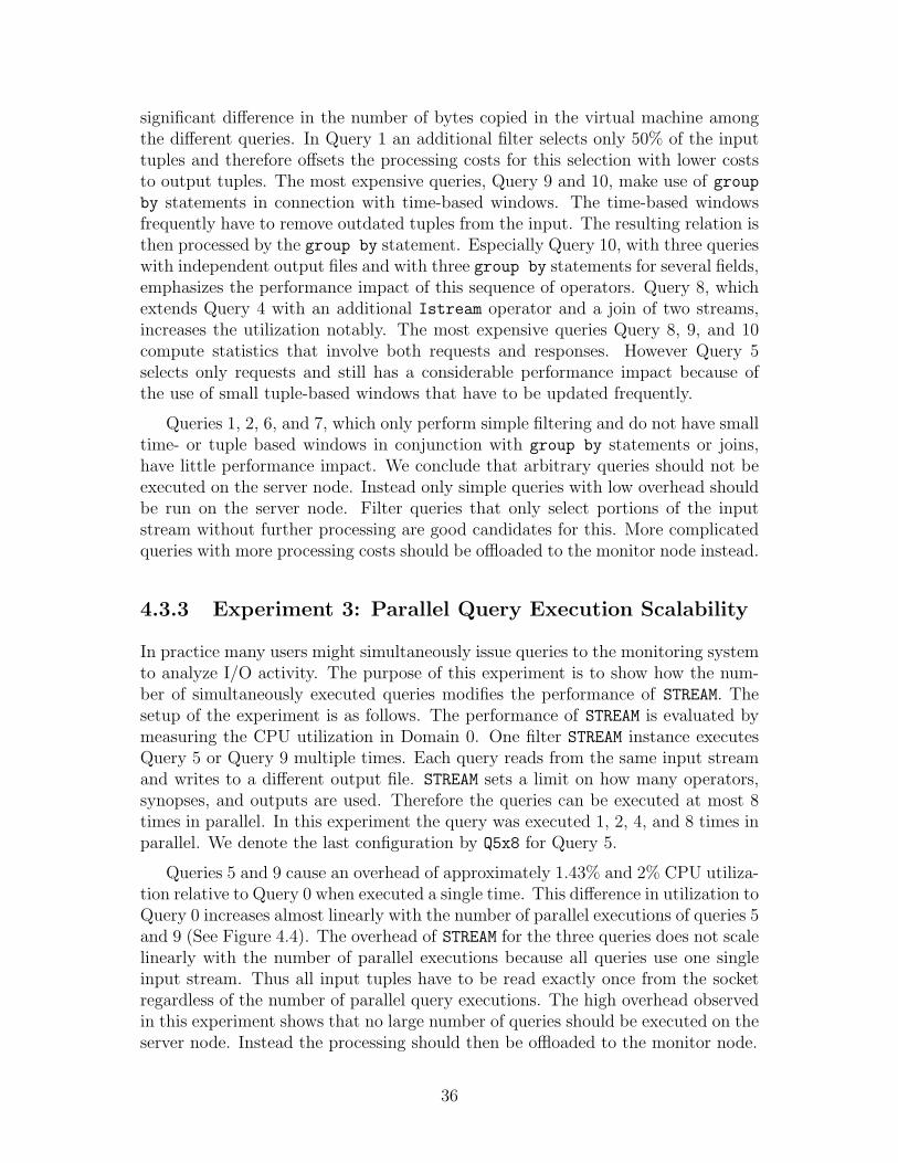
significant difference in the number of bytes copied in the virtual machine amongthe different queries. In Query 1 an additional filter selects only 50% of the inputtuples and therefore offsets the processing costs for this selection with lower coststo output tuples. The most expensive queries, Query 9 and 10, make use of groupby statements in connection with time-based windows. The time-based windowsfrequently have to remove outdated tuples from the input. The resulting relation isthen processed by the group by statement. Especially Query 10, with three querieswith independent output files and with three group by statements for several fields,emphasizes the performance impact of this sequence of operators. Query 8, whichextends Query 4 with an additional Istream operator and a join of two streams,increases the utilization notably. The most expensive queries Query 8, 9, and 10compute statistics that involve both requests and responses. However Query 5selects only requests and still has a considerable performance impact because ofthe use of small tuple-based windows that have to be updated frequently.

Queries 1, 2, 6, and 7, which only perform simple filtering and do not have smalltime- or tuple based windows in conjunction with group by statements or joins,have little performance impact. We conclude that arbitrary queries should not beexecuted on the server node. Instead only simple queries with low overhead shouldbe run on the server node. Filter queries that only select portions of the inputstream without further processing are good candidates for this. More complicatedqueries with more processing costs should be offloaded to the monitor node instead.

4.3.3 Experiment 3: Parallel Query Execution Scalability

In practice many users might simultaneously issue queries to the monitoring systemto analyze I/O activity. The purpose of this experiment is to show how the num-ber of simultaneously executed queries modifies the performance of STREAM. Thesetup of the experiment is as follows. The performance of STREAM is evaluated bymeasuring the CPU utilization in Domain 0. One filter STREAM instance executesQuery 5 or Query 9 multiple times. Each query reads from the same input streamand writes to a different output file. STREAM sets a limit on how many operators,synopses, and outputs are used. Therefore the queries can be executed at most 8times in parallel. In this experiment the query was executed 1, 2, 4, and 8 times inparallel. We denote the last configuration by Q5x8 for Query 5.

Queries 5 and 9 cause an overhead of approximately 1.43% and 2% CPU utiliza-tion relative to Query 0 when executed a single time. This difference in utilization toQuery 0 increases almost linearly with the number of parallel executions of queries 5and 9 (See Figure 4.4). The overhead of STREAM for the three queries does not scalelinearly with the number of parallel executions because all queries use one singleinput stream. Thus all input tuples have to be read exactly once from the socketregardless of the number of parallel query executions. The high overhead observedin this experiment shows that no large number of queries should be executed on theserver node. Instead the processing should then be offloaded to the monitor node.

36

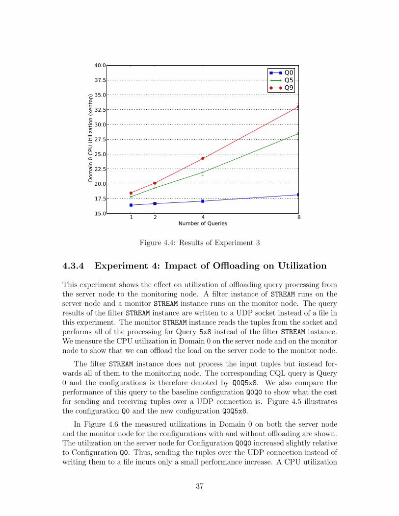
1 2 4 8Number of Queries

15.0

17.5

20.0

22.5

25.0

27.5

30.0

32.5

35.0

37.5

40.0

Dom

ain

0 C

PU

Uti

lizati

on (

xento

p)

Q0Q5Q9


4.3.4 Experiment 4: Impact of Offloading on Utilization

This experiment shows the effect on utilization of offloading query processing fromthe server node to the monitoring node. A filter instance of STREAM runs on theserver node and a monitor STREAM instance runs on the monitor node. The queryresults of the filter STREAM instance are written to a UDP socket instead of a file inthis experiment. The monitor STREAM instance reads the tuples from the socket andperforms all of the processing for Query 5x8 instead of the filter STREAM instance.We measure the CPU utilization in Domain 0 on the server node and on the monitornode to show that we can offload the load on the server node to the monitor node.

The filter STREAM instance does not process the input tuples but instead for-wards all of them to the monitoring node. The corresponding CQL query is Query0 and the configurations is therefore denoted by Q0Q5x8. We also compare theperformance of this query to the baseline configuration Q0Q0 to show what the costfor sending and receiving tuples over a UDP connection is. Figure 4.5 illustratesthe configuration Q0 and the new configuration Q0Q5x8.

In Figure 4.6 the measured utilizations in Domain 0 on both the server nodeand the monitor node for the configurations with and without offloading are shown.The utilization on the server node for Configuration Q0Q0 increased slightly relativeto Configuration Q0. Thus, sending the tuples over the UDP connection instead ofwriting them to a file incurs only a small performance increase. A CPU utilization

37

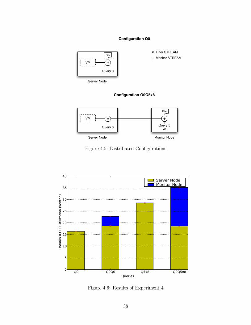
VM *

Query 0

Server Node

Configuration Q0

VM * +Query 0

Monitor NodeServer Node

Query 5x8

Configuration Q0Q5x8

+*Filter STREAMMonitor STREAM

File

File

Figure 4.5: Distributed Configurations

Q0 Q0Q0 Q5x8 Q0Q5x8Queries

0

5

10

15

20

25

30

35

40

Dom

ain

0 C

PU

Uti

lizati

on (

xento

p)

Server NodeMonitor Node


38

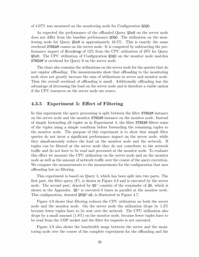
of 4.07% was measured on the monitoring node for Configuration Q0Q0.

As expected the performance of the offloaded Query Q5x8 on the server nodedoes not differ from the baseline performance Q0Q0. The utilization on the mon-itoring node for Query Q5x8 is approximately 16.5%. This is exactly the sameoverhead STREAM causes on the server node. It is computed by subtracting the per-formance impact of Blocktap of 12% from the CPU utilization of 28% for QueryQ5x8. The CPU utilization of Configuration Q0Q0 on the monitor node matchesSTREAM’s overhead for Query 0 on the server node.

The chart also contains the utilizations on the server node for the queries that donot employ offloading. The measurements show that offloading to the monitoringnode does not greatly increase the sum of utilizations in server and monitor node.Thus the overall overhead of offloading is small. Additionally offloading has theadvantage of decreasing the load on the server node and is therefore a viable optionif the CPU resources on the server node are scarce.

4.3.5 Experiment 5: Effect of Filtering

In this experiment the query processing is split between the filter STREAM instanceon the server node and the monitor STREAM instance on the monitor node. Insteadof simply forwarding all tuples as in Experiment 4, the filter STREAM filters someof the tuples using a simple condition before forwarding the remaining tuples tothe monitor node. The purpose of this experiment is to show that simple filterqueries do not incur a significant performance impact on the server node, whilethey simultaneously reduce the load on the monitor node and the network. Iftuples can be filtered at the server node they do not contribute to the networktraffic and do not have to be read and processed at the monitor node. To evaluatethis effect we measure the CPU utilization on the server node and on the monitornode as well as the amount of network traffic over the course of the query execution.We compare the measurements to the measurements for the configuration that usesoffloading but no filtering.

This experiment is based on Query 5, which has been split into two parts. Thefirst part, the filter query (F), is shown in Figure 4.8 and is executed by the servernode. The second part, denoted by Q5’ consists of the remainder of Q5, which isshown in the Appendix. Q5’ is executed 8 times in parallel at the monitor node.This configuration, denoted QFQ5’x8, is illustrated in Figure 4.7.

Figure 4.9 shows that filtering reduces the CPU utilization on both the servernode and the monitor node. On the server node the utilization drops by 1.2%because fewer tuples have to be sent over the network. The CPU utilization alsodrops by a small amount (1.8%) on the monitor node, because fewer tuples have tobe read from the UDP socket and the filter for requests is not executed.

Figure 4.9 also shows the bandwidth usage between the server and the moni-toring node over the course of the complete experiment for the offloading and the

39

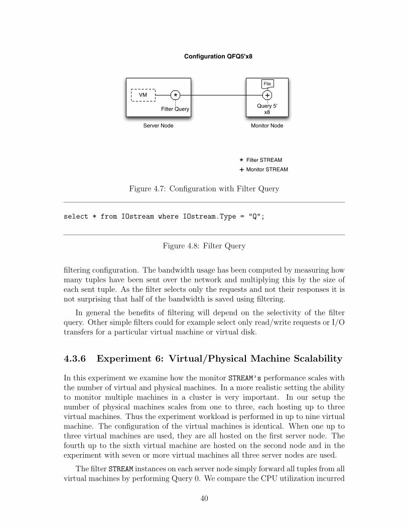
+*Filter STREAMMonitor STREAM

VM * +Filter Query

Monitor NodeServer Node

Query 5'x8

Configuration QFQ5'x8

File

Figure 4.7: Configuration with Filter Query

select * from IOstream where IOstream.Type = "Q";

Figure 4.8: Filter Query

filtering configuration. The bandwidth usage has been computed by measuring howmany tuples have been sent over the network and multiplying this by the size ofeach sent tuple. As the filter selects only the requests and not their responses it isnot surprising that half of the bandwidth is saved using filtering.

In general the benefits of filtering will depend on the selectivity of the filterquery. Other simple filters could for example select only read/write requests or I/Otransfers for a particular virtual machine or virtual disk.

4.3.6 Experiment 6: Virtual/Physical Machine Scalability

In this experiment we examine how the monitor STREAM’s performance scales withthe number of virtual and physical machines. In a more realistic setting the abilityto monitor multiple machines in a cluster is very important. In our setup thenumber of physical machines scales from one to three, each hosting up to threevirtual machines. Thus the experiment workload is performed in up to nine virtualmachine. The configuration of the virtual machines is identical. When one up tothree virtual machines are used, they are all hosted on the first server node. Thefourth up to the sixth virtual machine are hosted on the second node and in theexperiment with seven or more virtual machines all three server nodes are used.

The filter STREAM instances on each server node simply forward all tuples from allvirtual machines by performing Query 0. We compare the CPU utilization incurred

40

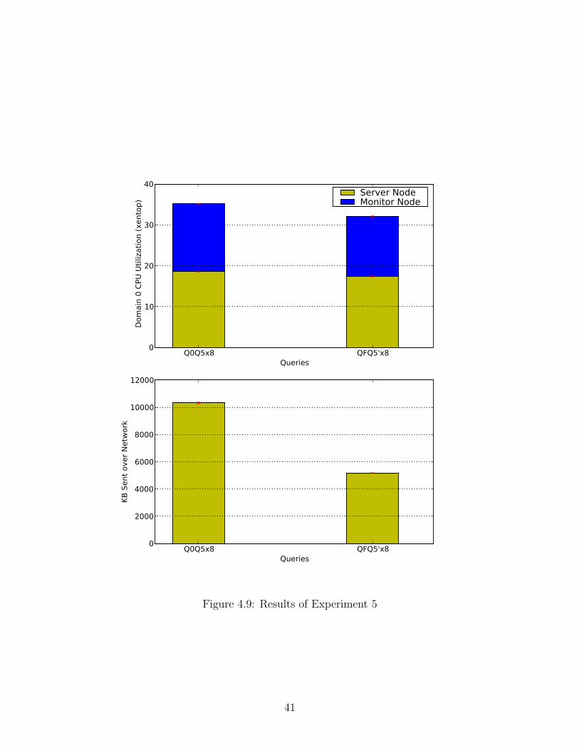
Q0Q5x8 QFQ5'x8Queries

0

10

20

30

40

Dom

ain

0 C

PU

Uti

lizati

on (

xento

p)

Server NodeMonitor Node

Q0Q5x8 QFQ5'x8Queries

0

2000

4000

6000

8000

10000

12000

KB

Sent

over

Netw

ork


41

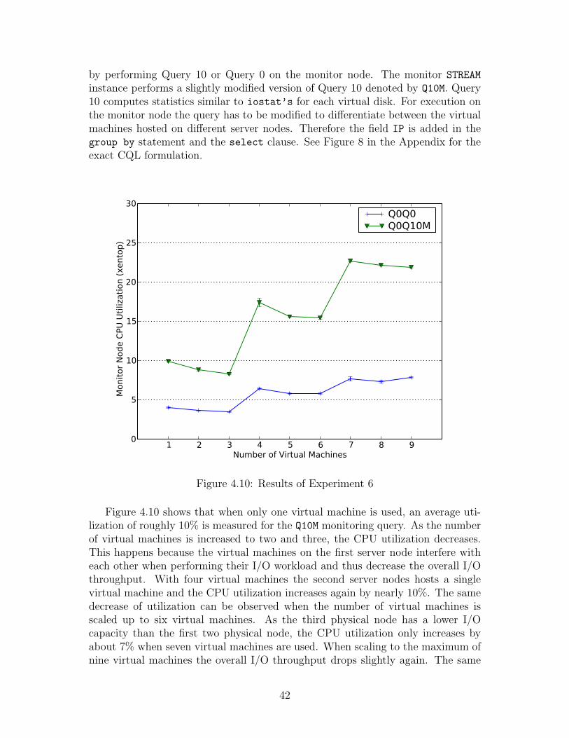
by performing Query 10 or Query 0 on the monitor node. The monitor STREAM

instance performs a slightly modified version of Query 10 denoted by Q10M. Query10 computes statistics similar to iostat’s for each virtual disk. For execution onthe monitor node the query has to be modified to differentiate between the virtualmachines hosted on different server nodes. Therefore the field IP is added in thegroup by statement and the select clause. See Figure 8 in the Appendix for theexact CQL formulation.

1 2 3 4 5 6 7 8 9Number of Virtual Machines

0

5

10

15

20

25

30

Monit

or

Node C

PU

Uti

lizati

on (

xento

p)

Q0Q0Q0Q10M


Figure 4.10 shows that when only one virtual machine is used, an average uti-lization of roughly 10% is measured for the Q10M monitoring query. As the numberof virtual machines is increased to two and three, the CPU utilization decreases.This happens because the virtual machines on the first server node interfere witheach other when performing their I/O workload and thus decrease the overall I/Othroughput. With four virtual machines the second server nodes hosts a singlevirtual machine and the CPU utilization increases again by nearly 10%. The samedecrease of utilization can be observed when the number of virtual machines isscaled up to six virtual machines. As the third physical node has a lower I/Ocapacity than the first two physical node, the CPU utilization only increases byabout 7% when seven virtual machines are used. When scaling to the maximum ofnine virtual machines the overall I/O throughput drops slightly again. The same

42

scaling behaviour can be observed when Query 0 is executed on the monitor nodeinstead of Query 10M.

We conclude that the performance of the monitoring system scales linearly withthe number of input tuples. The number of virtual machines does not affect theperformance negatively. When the workload is I/O-bound an increasing number ofvirtual machines interfere more and more and therefore the input rate to STREAM

decreases.

43

Chapter 5

Conclusions and Future Work

5.1 Conclusions

In this work we have contributed the following:

1. We designed a distributed, customizable I/O monitoring architecture. Tocreate a prototype implementation we have modified two existing pieces ofsoftware: Blocktap and STREAM. A facility for logging of I/O request metadatato Unix domain sockets has been added to Blocktap. For STREAM, input andoutput operators for UDP have been introduced. Example queries show thatthe architecture can be used for more flexible and detailed analysis of I/Otransfers.

2. We have performed experiments involving Blocktap and STREAM to analyzethe overhead of the prototype. For that, STREAM’s scheduler has been mod-ified to avoid busy-looping to make CPU utilization measurements possible.The results show that I/O monitoring can potentially cause significant over-head, but that by offloading query processing to a separate monitor node, theperformance impact on the server nodes can be minimized.

3. Additionally we have analyzed how simple filtering at the server nodes andperforming residual queries at the monitoring node can reduce the load onthe monitoring node and the volume of data sent over the network. Filteringdoes not require a significant amount of CPU resources.

5.2 Future Work

As a next step we would like to implement more data sources for I/O requests. Inthe course of the thesis we have determined that DTrace could probably be usedas an input source. Its current capabilities could thus be extended for distributed

44

and hopefully more flexible queries. With its probes in the Solaris kernel veryfine-grained analysis of I/O requests could be performed.

Another interesting project would be to improve the support for distributionin our system. A very interesting modification of STREAM would be support fordiffering schemata. Currently both DSMS instances share the same schema andno complicated queries that change the schema can be supported. A facility forchanging schemata would dramatically decrease the amount of data sent over thenetwork in some cases. We also would like to try to port our input sources to otherDSMSs with more support for distribution. For example Borealis would be onecandidate. It already has some notion of load-balancing and is perhaps able tosupport a more automated query optimization for our optimization goal.

Another goal is the design of an automated resource allocation mechanism usingqueries that signal poor performance. Currently Xen does not support fine-grainedscheduling of I/O resources, but we would like to build a basic mechanism forthis. Another approach to a self-tuning system could be to assign I/O intensiveworkloads to less utilized virtual machines. With the current system it might alsobe possible to devise a mechanism that analyzes a virtual machine workload andautomatically optimizes the storage configuration for this workload.

Some minor technical goals would be to improve the fault-tolerance and auton-omy of the system by introducing special control and error tuples to signal problemsto the STREAM instances.

45

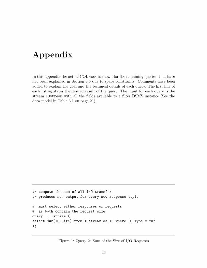
Appendix

In this appendix the actual CQL code is shown for the remaining queries, that havenot been explained in Section 3.5 due to space constraints. Comments have beenadded to explain the goal and the technical details of each query. The first line ofeach listing states the desired result of the query. The input for each query is thestream IOstream with all the fields available to a filter DSMS instance (See thedata model in Table 3.1 on page 21).

#- compute the sum of all I/O transfers

#- produces new output for every new response tuple

# must select either responses or requests

# as both contain the request size

query : Istream (

select Sum(IO.Size) from IOstream as IO where IO.Type = "R"

);

Figure 1: Query 2: Sum of the Size of I/O Requests

46

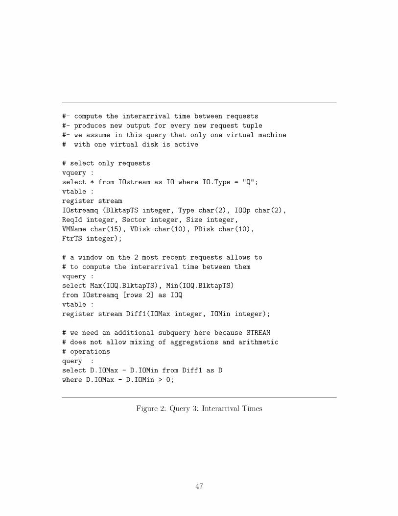
#- compute the interarrival time between requests

#- produces new output for every new request tuple



# select only requests

vquery :

select * from IOstream as IO where IO.Type = "Q";

vtable :

register stream

IOstreamq (BlktapTS integer, Type char(2), IOOp char(2),

ReqId integer, Sector integer, Size integer,

VMName char(15), VDisk char(10), PDisk char(10),

FtrTS integer);

# a window on the 2 most recent requests allows to

# to compute the interarrival time between them

vquery :

select Max(IOQ.BlktapTS), Min(IOQ.BlktapTS)

from IOstreamq [rows 2] as IOQ

vtable :

register stream Diff1(IOMax integer, IOMin integer);

# we need an additional subquery here because STREAM

# does not allow mixing of aggregations and arithmetic

# operations

query :

select D.IOMax - D.IOMin from Diff1 as D

where D.IOMax - D.IOMin > 0;

Figure 2: Query 3: Interarrival Times

47

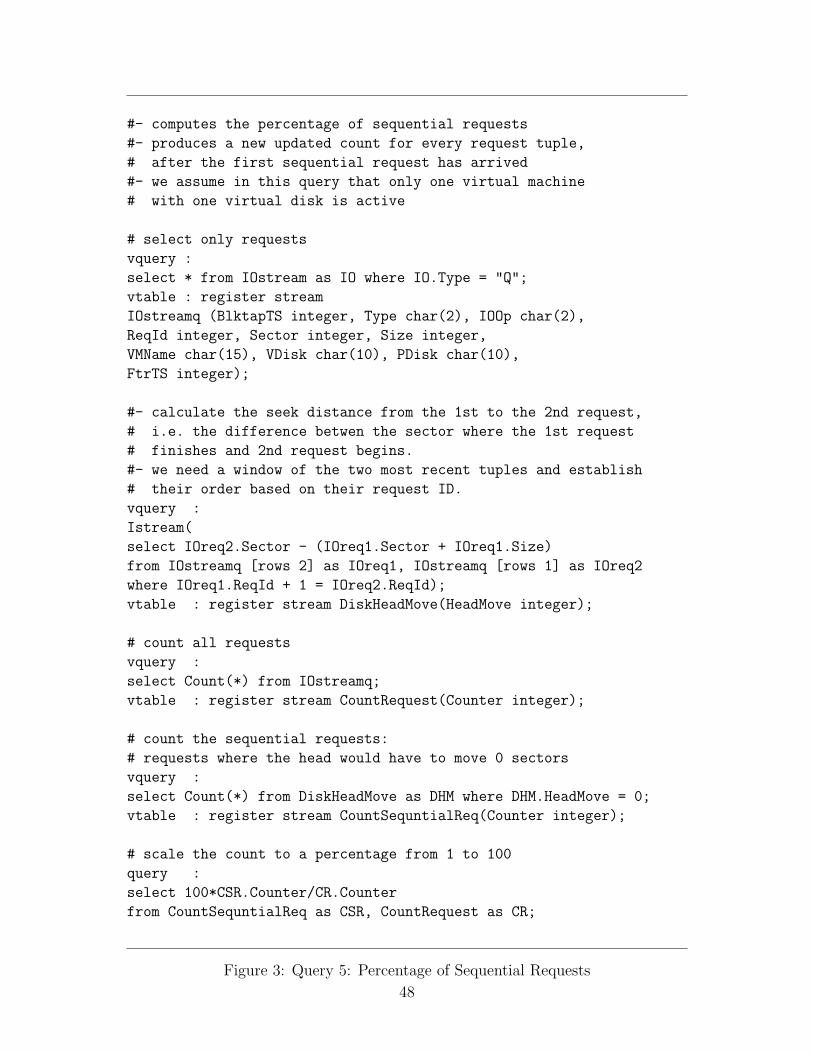
#- computes the percentage of sequential requests

#- produces a new updated count for every request tuple,

# after the first sequential request has arrived




vquery :






FtrTS integer);

#- calculate the seek distance from the 1st to the 2nd request,

# i.e. the difference betwen the sector where the 1st request

# finishes and 2nd request begins.

#- we need a window of the two most recent tuples and establish

# their order based on their request ID.

vquery :

Istream(

select IOreq2.Sector - (IOreq1.Sector + IOreq1.Size)

from IOstreamq [rows 2] as IOreq1, IOstreamq [rows 1] as IOreq2

where IOreq1.ReqId + 1 = IOreq2.ReqId);

vtable : register stream DiskHeadMove(HeadMove integer);

# count all requests

vquery :

select Count(*) from IOstreamq;

vtable : register stream CountRequest(Counter integer);

# count the sequential requests:

# requests where the head would have to move 0 sectors

vquery :

select Count(*) from DiskHeadMove as DHM where DHM.HeadMove = 0;

vtable : register stream CountSequntialReq(Counter integer);

# scale the count to a percentage from 1 to 100

query :

select 100*CSR.Counter/CR.Counter

from CountSequntialReq as CSR, CountRequest as CR;

Figure 3: Query 5: Percentage of Sequential Requests

48

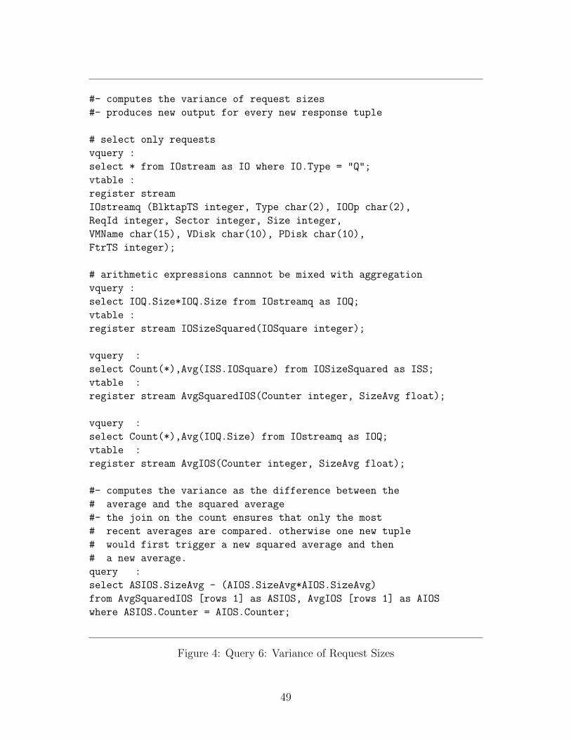
#- computes the variance of request sizes

#- produces new output for every new response tuple


vquery :


vtable :

register stream




FtrTS integer);

# arithmetic expressions cannnot be mixed with aggregation

vquery :

select IOQ.Size*IOQ.Size from IOstreamq as IOQ;

vtable :

register stream IOSizeSquared(IOSquare integer);

vquery :

select Count(*),Avg(ISS.IOSquare) from IOSizeSquared as ISS;

vtable :

register stream AvgSquaredIOS(Counter integer, SizeAvg float);

vquery :

select Count(*),Avg(IOQ.Size) from IOstreamq as IOQ;

vtable :

register stream AvgIOS(Counter integer, SizeAvg float);

#- computes the variance as the difference between the

# average and the squared average

#- the join on the count ensures that only the most

# recent averages are compared. otherwise one new tuple

# would first trigger a new squared average and then

# a new average.

query :

select ASIOS.SizeAvg - (AIOS.SizeAvg*AIOS.SizeAvg)

from AvgSquaredIOS [rows 1] as ASIOS, AvgIOS [rows 1] as AIOS

where ASIOS.Counter = AIOS.Counter;

Figure 4: Query 6: Variance of Request Sizes

49

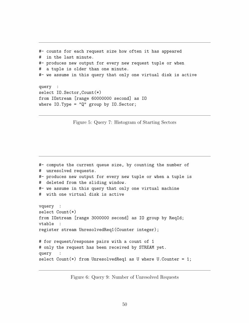
#- counts for each request size how often it has appeared

# in the last minute.

#- produces new output for every new request tuple or when

# a tuple is older than one minute.

#- we assume in this query that only one virtual disk is active

query :

select IO.Sector,Count(*)

from IOstream [range 60000000 second] as IO

where IO.Type = "Q" group by IO.Sector;

Figure 5: Query 7: Histogram of Starting Sectors

#- compute the current queue size, by counting the number of

# unresolved requests.

#- produces new output for every new tuple or when a tuple is

# deleted from the sliding window.



vquery :

select Count(*)

from IOstream [range 3000000 second] as IO group by ReqId;

vtable :

register stream UnresolvedReq1(Counter integer);

# for request/response pairs with a count of 1

# only the request has been received by STREAM yet.

query :

select Count(*) from UnresolvedReq1 as U where U.Counter = 1;

Figure 6: Query 9: Number of Unresolved Requests

50

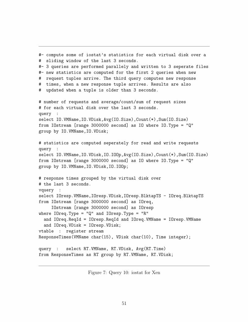
#- compute some of iostat’s statistics for each virtual disk over a

# sliding window of the last 3 seconds.

#- 3 queries are performed parallely and written to 3 seperate files

#- new statistics are computed for the first 2 queries when new

# request tuples arrive. The third query computes new response

# times, when a new response tuple arrives. Results are also

# updated when a tuple is older than 3 seconds.

# number of requests and average/count/sum of request sizes

# for each virtual disk over the last 3 seconds.

query :

select IO.VMName,IO.VDisk,Avg(IO.Size),Count(*),Sum(IO.Size)

from IOstream [range 3000000 second] as IO where IO.Type = "Q"

group by IO.VMName,IO.VDisk;

# statistics are computed seperately for read and write requests

query :

select IO.VMName,IO.VDisk,IO.IOOp,Avg(IO.Size),Count(*),Sum(IO.Size)


group by IO.VMName,IO.VDisk,IO.IOOp;

# response times grouped by the virtual disk over

# the last 3 seconds.

vquery :

select IOresp.VMName,IOresp.VDisk,IOresp.BlktapTS - IOreq.BlktapTS




and IOreq.ReqId = IOresp.ReqId and IOreq.VMName = IOresp.VMName

and IOreq.VDisk = IOresp.VDisk;


ResponseTimes(VMName char(15), VDisk char(10), Time integer);

query : select RT.VMName, RT.VDisk, Avg(RT.Time)

from ResponseTimes as RT group by RT.VMName, RT.VDisk;

Figure 7: Query 10: iostat for Xen

51

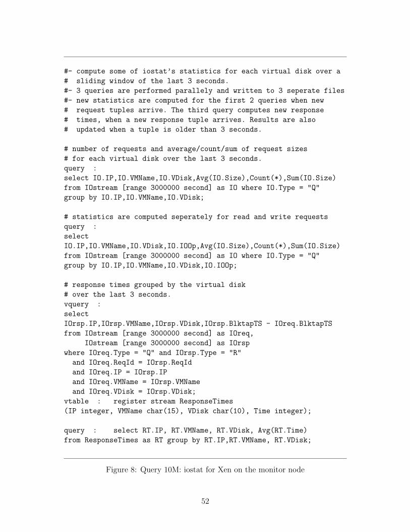
#- compute some of iostat’s statistics for each virtual disk over a

# sliding window of the last 3 seconds.

#- 3 queries are performed parallely and written to 3 seperate files

#- new statistics are computed for the first 2 queries when new

# request tuples arrive. The third query computes new response

# times, when a new response tuple arrives. Results are also

# updated when a tuple is older than 3 seconds.

# number of requests and average/count/sum of request sizes

# for each virtual disk over the last 3 seconds.

query :

select IO.IP,IO.VMName,IO.VDisk,Avg(IO.Size),Count(*),Sum(IO.Size)


group by IO.IP,IO.VMName,IO.VDisk;

# statistics are computed seperately for read and write requests

query :

select

IO.IP,IO.VMName,IO.VDisk,IO.IOOp,Avg(IO.Size),Count(*),Sum(IO.Size)


group by IO.IP,IO.VMName,IO.VDisk,IO.IOOp;

# response times grouped by the virtual disk

# over the last 3 seconds.

vquery :

select

IOrsp.IP,IOrsp.VMName,IOrsp.VDisk,IOrsp.BlktapTS - IOreq.BlktapTS


IOstream [range 3000000 second] as IOrsp

where IOreq.Type = "Q" and IOrsp.Type = "R"

and IOreq.ReqId = IOrsp.ReqId

and IOreq.IP = IOrsp.IP

and IOreq.VMName = IOrsp.VMName

and IOreq.VDisk = IOrsp.VDisk;

vtable : register stream ResponseTimes

(IP integer, VMName char(15), VDisk char(10), Time integer);

query : select RT.IP, RT.VMName, RT.VDisk, Avg(RT.Time)

from ResponseTimes as RT group by RT.IP,RT.VMName, RT.VDisk;

Figure 8: Query 10M: iostat for Xen on the monitor node

52

References

[1] Bochs project website. http://bochs.sourceforge.net/. Accessed on Jan29, 2009. 7

[2] CQL specification. http://infolab.stanford.edu/stream/code/

cql-spec.txt. Accessed on Mar 5, 2009. 24

[3] Hyper-v website. http://www.microsoft.com/windowsserver2008/en/us/

hyperv.aspx. Accessed on Jan 29, 2009. 7

[4] OpenVZ website. http://www.openvz.org. Accessed on Jan 29, 2009. 7

[5] Parallels website. http://www.parallels.com/. Accessed on Jan 29, 2009. 7

[6] STREAM manual. http://www-db.stanford.edu/stream/code/user.pdf.Accessed on Mar 5, 2009. 24

[7] VirtualBox website. http://www.virtualbox.org/. Accessed on Jan 29,2009. 7

[8] Website on IBM virtualization solutions. http://www.ibm.com/systems/

virtualization/. Accessed on Jan 29, 2009. 7

[9] Daniel J. Abadi, Yanif Ahmad, Magdalena Balazinska, Ugur Cetintemel, MitchCherniack, Jeong-Hyon Hwang, Wolfgang Lindner, Anurag Maskey, AlexRasin, Esther Ryvkina, Nesime Tatbul, Ying Xing, and Stanley B. Zdonik.The Design of the Borealis Stream Processing Engine. In Conference on In-novative Data Systems Research (CIDR), pages 277–289, 2005. 14

[10] U.S. Environmental Protection Agency. Report to congress on server and datacenter energy efficiency. Public Law 109-431, August 2007. 7

[11] Yanif Ahmad, Bradley Berg, Ugur Cetintemel, Mark Humphrey, Jeong-HyonHwang, Anjali Jhingran, Anurag Maskey, Olga Papaemmanouil, Alex Rasin,Nesime Tatbul, Wenjuan Xing, Ying Xing, and Stanley B. Zdonik. Distributedoperation in the Borealis stream processing engine. In ACM Special InterestGroup on Management of Data (SIGMOD) Conference, pages 882–884, 2005.16

53

http://bochs.sourceforge.net/

http://infolab.stanford.edu/stream/code/cql-spec.txt

http://infolab.stanford.edu/stream/code/cql-spec.txt

http://www.microsoft.com/windowsserver2008/en/us/hyperv.aspx

http://www.microsoft.com/windowsserver2008/en/us/hyperv.aspx

http://www.openvz.org

http://www.parallels.com/

http://www-db.stanford.edu/stream/code/user.pdf

http://www.virtualbox.org/

http://www.ibm.com/systems/virtualization/

http://www.ibm.com/systems/virtualization/

[12] Arvind Arasu, Shivnath Babu, and Jennifer Widom. The CQL continu-ous query language: semantic foundations and query execution. Very LargeDatabases (VLDB) Journal, 15(2):121–142, 2006. 15, 24

[13] Brian Babcock, Shivnath Babu, Mayur Datar, Rajeev Motwani, and JenniferWidom. Models and issues in data stream systems. In Symposium on Principlesof Database Systems (PODS), pages 1–16, 2002. 3, 14, 16

[14] Paul Barham, Boris Dragovic, Keir Fraser, Steven Hand, Timothy L. Harris,Alex Ho, Rolf Neugebauer, Ian Pratt, and Andrew Warfield. Xen and the art ofvirtualization. In ACM Symposium on Operating Systems Principles (SOSP),pages 164–177, 2003. 7, 8

[15] Fabrice Bellard. QEMU, a fast and portable dynamic translator. In USENIXAnnual Technical Conference, pages 41–46, 2005. 7

[16] Michael Cammert, Christoph Heinz, Jurgen Kramer, Alexander Markowetz,and Bernhard Seeger. PIPES: A multi-threaded publish-subscribe architecturefor continuous queries over streaming data. Technical Report 50, Philipps-University Marburg, 2003. 14

[17] Bryan Cantrill, Michael W. Shapiro, and Adam H. Leventhal. Dynamic instru-mentation of production systems. In USENIX Annual Technical Conference,pages 15–28, 2004. 2, 5

[18] Sirish Chandrasekaran, Owen Cooper, Amol Deshpande, Michael J. Franklin,Joseph M. Hellerstein, Wei Hong, Sailesh Krishnamurthy, Samuel Madden,Vijayshankar Raman, Frederick Reiss, and Mehul A. Shah. TelegraphCQ:Continuous dataflow processing for an uncertain world. In Conference onInnovative Data Systems Research (CIDR), 2003. 14

[19] Alvin Cheung and Samuel Madden. Performance profiling with EndoScope,an acquisitional software monitoring framework. Proceedings of the VLDBEndowment (PVLDB), 1(1):42–53, 2008. 16

[20] David Chisnall. The Definitive Guide to the Xen Hypervisor. Prentice Hall,2007. 8, 9, 12, 23

[21] collecti website. http://collecti.sourceforge.net. Accessed on Sep 1,2008. 5

[22] Jeff Dike. A user-mode port of the Linux kernel. In 4th Annual Linux Showcase& Conference, November 2000. 7

[23] Keir Fraser, Steven Hand, Rolf Neugebauer, Ian Pratt, Andrew Warfield, andMark Williamson. Safe hardware access with the Xen virtual machine monitor.In Workshop on Operating System and Architectural Support for the on demandIT InfraStructure (OASIS), 2004. 11

54

http://collecti.sourceforge.net

[24] Juan Garcia and David E. Williams. Virtualization with Xen. Syngress, May2007. 10

[25] Lukasz Golab and M. Tamer Ozsu. Issues in data stream management. SpecialInterest Group on the Management of Data (SIGMOD) Record, 32(2):5–14,2003. 14, 15

[26] The STREAM Group. STREAM: The Stanford Stream Data Manager. Tech-nical Report 2003-21, Stanford InfoLab, 2003. 14, 15

[27] Raj Jain. The Art of Computer Systems Performance Analysis. John Wiley& Sons, Inc, 2nd edition, April 1991. 1

[28] Poul-Henning Kamp and Robert N. M. Watson. Jails: Confining the omnipo-tent root. May 2000. 7

[29] KDB+ website. http://kx.com/products/database.php. Accessed on Sep1, 2008. 15

[30] Linux iostat Manpage, November 2005. Part of sysstat version 6.0.2. 4

[31] Mac OS X fs usage Manpage, November 2002. 5

[32] Mac OS X sc usage Manpage, October 2002. 5

[33] Jeanna Neefe Matthews, Wenjin Hu, Madhujith Hapuarachchi, Todd Deshane,Demetrios Dimatos, Gary Hamilton, Michael McCabe, and James Owens.Quantifying the performance isolation properties of virtualization systems. InExperimental Computer Science, page 6, 2007. 7

[34] Erin McKean, editor. The New Oxford American Dictionary. Oxford Univer-sity Press, USA, 2nd edition, May 2005. 1

[35] Dutch T. Meyer, Brendan Cully, Jake Wires, Norman C. Hutchinson, and An-drew Warfield. Block Mason. In Workshop on I/O Virtualization (WIOV’08),December 2008. 14

[36] Jun Nakajima and Asit K. Mallick. Hybrid Virtualization - Enhanced Virtu-alization for Linux. In Linux Symposium, June 2007. 9

[37] Gerald J. Popek and Robert P. Goldberg. Formal requirements for virtualizablethird generation architectures. Communications of the ACM, 17(7):412–421,1974. 8

[38] Daniel Price and Andrew Tucker. Solaris Zones: Operating System Supportfor Consolidating Commercial Workloads. In Large Installation System Ad-ministration Conference, pages 241–254, 2004. 7

[39] Qumranet. KVM – Kernel-based Virtualiztion Machine. 2006. 7

55

http://kx.com/products/database.php

[40] StreamBase website. http://www.streambase.com/. Accessed on Jan 29,2009. 14

[41] VMware. Understanding Full Virtualization, Paravirtualization, and HardwareAssist. 2007. 7

[42] VMware. VProbes Programming Reference, August 2008. http://www.

vmware.com/products/beta/ws/vprobes_reference.pdf. 6

[43] Andrew Warfield. Virtual Devices for Virtual Machines. PhD thesis, Universityof Cambridge, February 2006. 12

[44] Andrew Warfield and Julian Chesterfield. blktap readme, June 2006. http:

//lxr.xensource.com/lxr/source/tools/blktap/README. 10

[45] Andrew Warfield, Steven Hand, Keir Fraser, and Tim Deegan. Facilitating thedevelopment of soft devices. In USENIX Annual Technical Conference, pages379–382, 2005. ix, 11, 12, 13

[46] Andrew Whitaker, Marianne Shaw, and Steven D. Gribble. Denali: a scal-able isolation kernel. In ACM Special Interest Group on Operating Systems(SIGOPS) Conference, pages 10–15, 2002. 8

[47] Ying Xing, Stanley B. Zdonik, and Jeong-Hyon Hwang. Dynamic load distri-bution in the Borealis stream processor. In International Conference on DataEngineering (ICDE), pages 7910–802, 2005. 16, 19

[48] Yunyue Zhu and Dennis Shasha. StatStream: Statistical monitoring of thou-sands of data streams in real time. In International Conference on Very LargeData Bases (VLDB), pages 358–369, 2002. 15

56

http://www.streambase.com/

http://www.vmware.com/products/beta/ws/vprobes_reference.pdf

http://www.vmware.com/products/beta/ws/vprobes_reference.pdf

http://lxr.xensource.com/lxr/source/tools/blktap/README

http://lxr.xensource.com/lxr/source/tools/blktap/README

Documents

Flexible Monitoring of Storage I/O