AD-AO87 858 wILLIAMS COLL WILLIAMSTOWN MASS F/6 4/2COASTAL STORM MODEL.(U)

U ' RAPR 76 W T FOX, R A DAVIS N0001 69C--0151

| U N C L A S S F E D T R - 1 4 ml

'flfl/llflffllffllfElhhEEEEEElhEEmBhElhhElIEIII~lllElhEEEllI

lllEEE'....l{

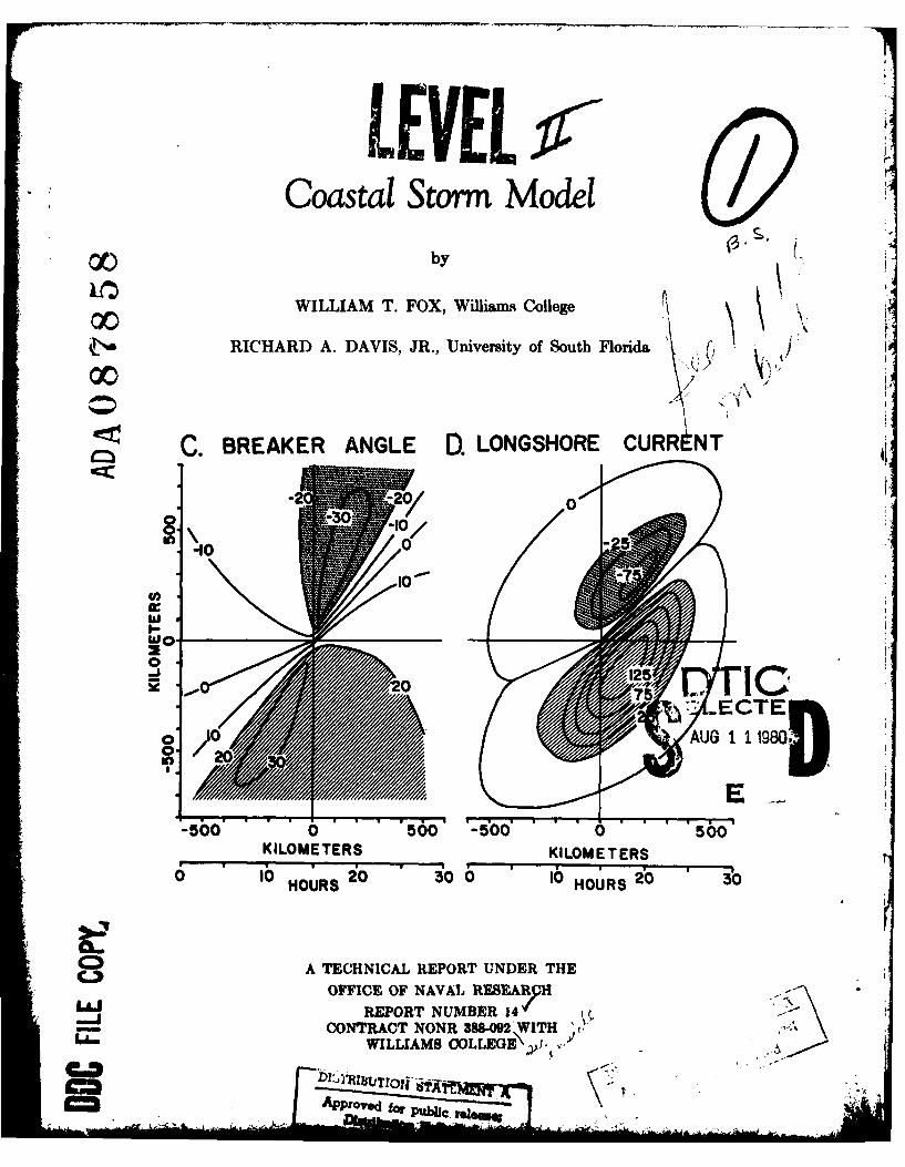
LEVELCoastal Storm Model

(Z) by

WILLIAM T. FOX, Williamm College

RICHARD A. DAVIS, JR., University of South Florida

C. BREAKER ANGLE D. LONGSHORE CURRENT

.1 -0 0 .

10

to0,

.. o'S,,. o ECTEh

-500 0 500 -500 0 500KILOMETERS KILOMETERS

ib o3 lbo i 'HOURS Io) HOURS 20

o A TECHNICAL REPORT UNDER THEC.>

OFFICE OF NAVAL RE8EARHLLJ REPORT NUMBER 14 VH

CONTrRACT NONR 388-092'WITHWILLIAMS 0OLLEGE\J ,...

. . .,, .ApprO. d fr .

II

COASTAL STORM MODEL

by

William T. Fox

and

Richard A. Davis, Jr.

Technical Report No. 14, April 30, 1976

of

ONR Task No. 388-092/10-18-68(414)

Contract N00014-69-C-0151 V

Office of Naval Research

ZfEL ~

Williams College

Will iamstown, Massachusetts

This report has been made possible through supportand sponsorship by the United States Department ofthe Navy, Office of Naval Research, under ONR TaskNumber 388-092, Contract N00014-69-C-0151. Repro-duction in whole or in part is permitted for anypurpose by the United States Government.

A . t fr public Tel al(3 ;

)' istilbution Unlimited

ABSTRACT

,A mathematical simulation model of a coastal storm has beenprogrammed to forecast or hindcast wave and longshore current con-ditions at a coastal site. Storm parameters for the model arebased on the size, shape intensity and path of the storm as de-rived from weather maps. An elliptical form is used to model thesize and shape of the storm which are controlled by varying thelength and orientation of the major and minor axes. Storm in-tensity is a function of the barometric pressure gradient whichis modeled by an inverted normal curve through the storm center.The storm path is based on actual storm positions for the hind-cast mode, and on projected positions assuming constant speedand direction for the forecast mode. The location, shorelineorientation and nearshore bottom slope provide input data foreach coastal site.

For each storm position, the geostrophic wind speed and di-rection are computed at the shore site as a function of baro-metric pressure gradient and latitude. The geostrophic wind isconverted into surface wind speed and direction by applyingcorrections for frictional effects over land and sea. IThe sur-face wind speed, fetch and duration are used to comput the waveperiod, breaker height and breaker angle at the shore ste. Thelongshore current velocity is computed as a function of waveperiod, breaker height and angle and nearshore bottom slope.

The model was tested by comparing hindcast output with ob-served data for several coastal locations. Forecasts were madefor actual storms and for hypothetical circular and ellipticalshaped storms.

Accession 'or

NTIS GFA&I£DC TAB

iU!]:I} t ri IC t t .JustiIic tion ___ '__

Ey

I :-t spcc Ial

". """°'v Code

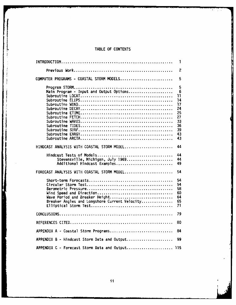
TABLE OF CONTENTS

INTRODUCTION ................................................ 1I

Previous Work........................................... 2

COMPUTER PROGRAMS - COASTAL STORM MODELS....................... 5

Program STORM........................................... 5Main Program - Input and Output Options .................... 6Subroutine LOCAT........................................ 11Subroutine ELIPS........................................ 14Subroutine WIND......................................... 17Subroutine DECAY........................................ 24Subroutine ETIME........................................ 25Subroutine FETCH........................................ 27ISubroutine WAVES........................................ 33Subroutine TIDES........................................ 36Subroutine SURF......................................... 39Subroutine ENRGY........................................ 43Subroutine ARCTA........................................ 43

HINDCAST ANALYSIS WITH COASTAL STORM MODEL..................... 44

Hindcast Tests of Models ................................ 44Stevensville, Michigan, July 1969.................... 44Additional Hindcast Examples ........................ 49

FORECAST ANALYSIS WITH COASTAL STORM MODEL..................... 54

Short-term Forecasts .................................... 54Circular Storm Test..................................... 54Barometric Pressure..................................... 58Wind Speed and Direction ................................ 60Wave Period and Breaker Height........................... 64Breaker Angles and Longshore Current Velocity .............. 65Elliptical Storm Test ................................... 71

CONCLUSIONS................................................. 79

REFERENCES CITED ............................................ 80

APPENDIX A - Coastal Storm Programs ........................... 84

APPENDIX B - Hindcast Storm Data and Output.................... 99

APPENDIX C - Forecast Storm Data and Output ................... 115

LIST OF FIGURES

Figure 1. Location map of field sites designated by project year ....... 3

2. A. Map coordinate system (X-Y) for locating stormcenter and shore site, and B. Storm coordinate system(Xl-Yl) with origin at storm center and X axis parallelto the shore ................................................. 13

3. Location of the shore site (X1,Y1) within a storm ellipse(AB) and on a minor ellipse (Al,Bl) .......................... 15

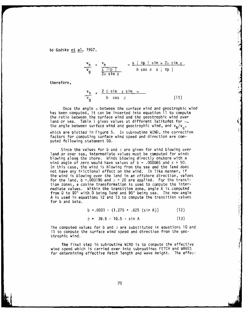
4. Orientation of the frictional force near the surface ofthe earth (Godske, et al, 1957, p. 453) ...................... 19

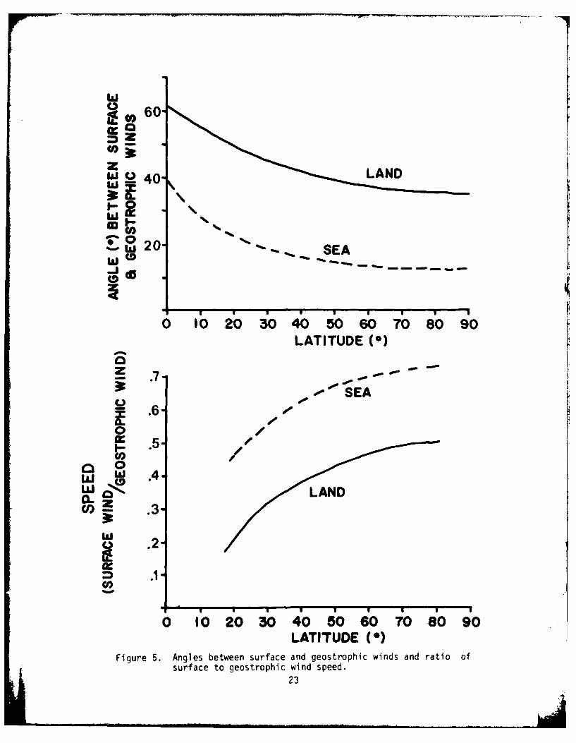
5. Angle between surface and geostrophic winds and ratio ofsurface to geostrophic wind speed ............................ 23

6. Case 1 - storm fetch when the distance from center of stormX is less than 1/3 storm radius, R ........................... 29

7. Case 2 - storm fetch when the distance from center of storm..30X is less than 0.4444 and greater than 1/3 storm radius, R.

8. Case 3 - storm fetch when the distance from center of stormX is greater than 0.4444 storm radius, R .................... 31

9. Deepwater wave forecasting curves as a function of windspeed, fetch length and wind duration based on the S.M.B.method ....................................................... 35

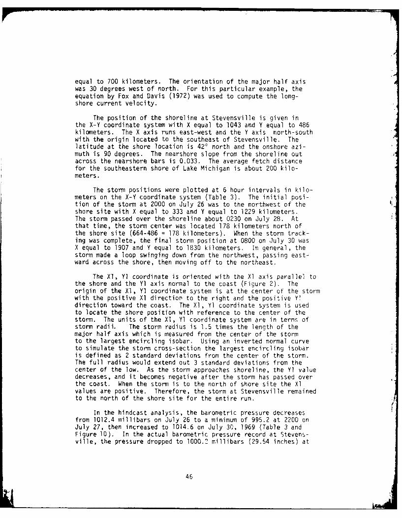
10. Observed and hindcast curves for barometric pressure, windvelocity, longshore current and breaker height at Stevens-ville, Michigan, July 26-30, 1969 ............................ 47

11. Observed and hindcast curves for Holland, Michigan, July3-5, 1970 .................................................... 50

12. Observed and hindcast curves for Holland, Michigan, July18-20, 1970 .................................................. 51

13. Observed and hindcast curves for Sheboygan, Wisconsin,July 16-18, 1972 ............................................. 52

14. Observed and hindcast curves for Sheboygan, Wisconsin,July 22-26, 1972 ............................................. 53

15. Map of storm tracks and time-distance plot of barometricpressure for a circular storm ................................ 57

ii

Figure 16. Time-distance plot of barometric pressure and pressureprofiles 200 km north, over the site, and 200 km southof the site ........................................... 59

17. Time-distance plot of surface wind speed and three pro-files of wind speed in a circular storm .................. 59

18. Time-distance plots of A - surface wind speed, B - winddirection, C - onshore wind, and D - alongshore wind ina circular storm....................................... 63

19. Time-distance plot of breaker height and three profilesof breaker height in a circular storm.................... 67

20. Time-distance plot of longshore current and three profilesof longshore current in a circular storm ................. 67

21. Time-distance plot of A -wave period, B - breaker height,C - breaker angle, and D -longshore current in a circularstorm................................................. 69

22. Time-distance plot of barometric pressure in an ellipticalstorm................................................. 73

23. Time-distance plot of A - surface wind speed, B - winddirection, C - onshore wind and D - alongshore wind inan elliptical storm .................................... 75

24. Time-distance plot of A - wave period, B - breaker height,C - breaker angle and D - longshore current in an ellip-tical storm ........................................... 77

iv

ACKNOWLEDGEMENTS

We would like to acknowledge the cooperation and financialassistance of the Geography Programs, Office of Naval Research.We would also like to express our appreciation to the 30 under-graduate and graduate students from Williams College, Universityof South Florida, Western Michigan University, University ofTexas and Oregon State University who participated in variousaspects of the field projects which provided a foundation forthe coastal stormi model.

Thomas Getz of Williams College deveioped some of the sub-outines and provided significant input in the theory and appli-

cation of the computer simulation model. Douglas Rosen of theUniversity of South Florida assisted in drafting several of theillustrations. Annie Laliberte typed and proofread the manu-script.

V

COASTAL STORM MODEL

INTRODUCTION

Coastal storms which provide a combination of high winds,pounding waves and rapid longshore currents are a major cause ofdistructive erosion along beaches and cliffs. Beaches which aregenerally composed of sand or cobbles are subject to sudden changesduring storms. During one storm at Chesil Bank near Abbotsbury,England, the crest of a shingle beach was cut back 1.53 meters in3 hours (Lewis, 1931). During a severe storm in July 1969 atStevensville, Michigan, the beach and bluff were eroded back over5.5 meters when the waves reached a height of 2 meters (Fox andDavis, 1970b). On the Oregon coast, a beach was stripped of a2 meter thick blanket of sand and the wave cut terrace was exposedwhen the waves reached heights of 8 meters during late Novemeberstorms (Fox and Davis, 1974).

For any operation involving the coastal zone, it is essentialto make predictions of wave and current conditions during a coastalstorm. General wave forecasts on a worldwide grid are availablefrom the National Weather Service and Fleet Numerical Weather Center.These forecasts provide accurate predictions of wave conditions onthe open ocean, but do not provide detailed enough predictions forthe coastal zone. Therefore, a computer simulation model was de-veloped to fill the gap between wave predictions on the open oceanand surf predictions along the coast.

The coastal storm model utilizes an ellipse to simulate a mapof barometric pressure. The shape of the storm can be modifiedby varying the length and orientation of the major and minor axesof the ellipse. The intensity of the storm is controlled by in-creasing or decreasing the range in barometric pressure. The actualstorm track and dimensions are read in as data for hindcasting waveand current conditions. For making forecasts, the size, shape andintensity of the storm are provided as input data for the model. Inforecasting, the storm path is plotted by assuming a constant azimuthand velocity.

One of the initial steps in developing a coastal storm model isdetermination of the barometric pressure gradient at any point on theground surface under the storm. The pressure gradient is then usedin conjunction with the latitude to calculate the geostrophic windspeed, which in turn is used to compute the surface wind speed, waveheight and longshore current velocity. in the model, it is assumedthat a profile of barometric pressure along the major or minor axisof the storm ellipse can be represented by an inverted normal curve,By rotating the normal curve around the ellipse and taking the deriv-ative, it is possible to calculate the pressure gradient at any pointon the ground. From that point on, conventional methods are employedfor determining the geostrophic wind speed, surface wind speed, waveheight and longshore current velocity.

PREVIOUS WORK

The coastal storm model is based on a series of detailed fieldstudies which extended from 1969 through 1975. The studies inclu-ded the analysis and synthesis time-series data on barometric pres-sure,wind speed and direction, wave period and height and longshorecurrent velocity for 15 days to 1 year. Topographic profiles acrossthe beach and nearshore area were used to construct topographic mapsand maps of erosion and deposition. The sites in the study areplotted by datein Figure I and included in the following list alongwith references for each study.

1969 Stevensville, Michigan Fox and Davis, 1970a, 1970b

1970 Holland, Michigan Fox and Davis, 1971aDavis and Fox, 1971

1971-2 Mustang Island, Texas Davis and Fox, 1972c

Davis and Fox, 1975

1972 Sheboygan, Wisconsin Fox and Davis, 1972

1973 Cedar Island, Virginia Davis and Fox, 1974a

1973-4 South Beach, Oregon Fox and Davis, 1974

1974 Zion, Illinois Davis and Fox, 1974b

1974 South Haven, Michigan Davis and Fox, 1974b

1975 Plum Island, Massachusetts

The models have evolved from a geometric model called thearea-time prism (Davis and Fox, 1972a) through a conceptual model(Davis and Fox,1972b) to a process-response model for Lake Michigan(Fox and Davis, 1971b and 1973 ). The simulation model developedfor Lake Michigan was limited to the local geographic area wherethe storms moved directly onshore to the north of the study area.The proposed coastal storm model is an outgrowth of the earliermodel but is more generalized with broader application under awider range of storm conditions and shoreline orientations.

Several different types of computer models have been proposedfor the coastal environment. Probablistic models were developed toreproduce gross coastal features such as a recurved spit on thesouth coast of England (McCallagh and King, 1970) and the MississippiRiver Delta (McCammon, 1971). A markov process was used to simu-late the sequence of bar formation and migration across a beach

2

125 120 115 110 105 100 95 50 65 s 70

-4 -- ---

117 974

303

rV

(Sonu and van Beek. 1971). A deterministic model resembling awave tank experiment was proposed to simulate the interactionbetween a prograding delta and waves (Komar, 1973). A statis-tical model with a relatively simple beach topography to computebreaker height, longshore current velocity and wave setup (Collins,1971) was followed by a more deterministic approach to model thenearshore circulation patterns employing monochromatic waves andmore complex beach topographies (Noda, et al, 1974). An explicitfinite difference model for predicting time-dependent, wave in-duced nearshore circulation was developed by Birkemeier andDalrymple (1976).

On a larger scale, Resio and Hayden (1973) proposed an inte-grated storm model which combines three scales of atmospheric mo-tion, large scale, synoptic scale and small scale into an estima-tion of a winter wave-surge climate for the mid-Atlantic coast.At a similar scale, Goldsmith, et al (1974) developed a wave cli-mate model for the mid-Atlantic coat by using Dobson's (1967)wave refraction program to project offshore waves into the coastalzone.

The coastal storm model proposed in this report provides alink between the large-scale, seasonal wave-climate models andthe dynamic surf zone models. By tracking a storm across a shore-line, the wave parameters which are output from the storm modelfurnish input for the surf zone models. Therefore, the proposedstorm model could be combined with other computer models to pro-vide an integrated process model for the coastal zone.

4

COMPUTER PROGRAMS -COASTAL STORM MODEL

Program STORM

Program STORM is a mathematical simulation model which has

been programmed for the computer to forecast or hindcast waveIconditions at a coastal site during a storm. The 6ctual stormas represented by the isobars on a weather map is modeled byan elliptical storm with major and minor axes at right anglesand passing through the center of the low. The size, shape,intensity and path of the storm as determined from weather mapsare used to generate the surface wind pattern, wave height andperiod, and longshore current velocity as the storm moves acrossthe coast.

The computer program is divided into a main program, STORM,and a series of 11 subroutines. The main program is used to read4in the data, call the various subroutines for computing the wind,wave and current conditions, print out the predictions at one hourintervals. All the input and output is handled by the main pro-gram while the calculations are carried out by the various sub-routines. In this way, any portion of the model can be indepen-dently tested by using a small main program to call each subrou-tine individually. Therefore, if any problem arises in the mainprogram, it can be narrowed down to a particular subroutine, andthat subroutine can be tested under a variety of conditions with-out using the main program. Also, if a portion of the simulationmodel is to be incorporated into another program, any of the indi-vidual subroutines can be removed and used separately with theappropriate calling arguments.

The theory and mechanics of the program will be explained indetail starting with the MAIN program and proceeding through eachof the subroutines as they are called by the MAIN program. Theprogram was written in FORTRAN IV for an 8k IBM 1130 at WilliamsCollege. A full listing of the programs with appropriate commentcards is included in Appendix A. A second version of the MAIN pro-gram was written for the Xerox 530 which includes a graphics pack-age for a 29 inch plotter. The graphics package is used to plotbarometric pressure, surface wind, onshore wind, alongshore wind,breaker height, wave period and longshore current.

5

Main Program - Input and Output Options

The main program is used to read the input data for the stormand shoreline conditions, call the various subroutines and printout the results at one hour intervals. A listing of the input cardsis included in Appendix I with a description of each of the inputvariables. The program is dimensioned to make predictions up to130 hours or 5 days and 10 hours. If a longer prediction is desired,it is necessary to increase the dimension of U(130) and V(130) tothe required number of hours. In the model, 130 hours was selectedbecause of core limitations on the 8k IBM 1130. For most of thestorms, the 130 hour limitation was not a serious constriction,however, a larger dimension statement would be helpful in some cases.

The first two data cards are used to read in the title, startingtime, date and input/output options. The title used for the locationof the shore site can be up to 80 spaces long filling card 1. Onthe second card, the starting hour, ISTRT, is included in columns 1and 2 followed by the date, DAY, in columns 3 to 22. The startingtime is read in as an interger and must be right justified. If ISTRTis read in as 0, the program will terminate. For the input option,INAUT, in column 23, a 0 is used for metric units and a 1 is usedfor nautical units including nautical miles, knots, and feet per sec-ond. The output option, NAUT, in column 24 is separate from the in-put option but uses the same code, 0 for metric units and 1 for nau-tical units. Although metric units are becoming the standard andare now required for scientific reports, it may be desirable at timesto have the input or output in nautical units. With separate inputand output options, it is possible to have the input in metric ornautical units and convert to the other units with the output.

The first 3 columns of card 3 are used to select the majoroptions for the program. For the first option, INOPT, a 1 in column1 will call the hindcasting mode, while a 2 in column 1 will callthe forecasting mode. The hindcasting mode is used when storm posi-tions are available at six hour intervals. The hourly positions ofthe storm are determined by a linear interpolation between the 6-hourpositions. For the forecasting mode, the initial position of the stormalong with a constant velocity and azimuth are used to calculatesuccessive positions at 1-hour intervals. The variables for thehindcasting and forecasting modes are read in on card 6. The secondoption on card 3 is the tide prediction option, IFTID. If a 0 ispunched in column 2, the tide prediction option is suppressed andcard 4 is not included in the data set. The tide option is omittedfor a non-tidal body of water, such as the Great Lakes. Where tidedata are available from the tide tables or from observations, a 1is punched in column 2, and the tide data are included on card 4.The longshore current equation for the simulation run is selectedin option 3, LSCOP. Four different longshore current equations areincluded, (1) Fox and Davis (1972), (2) Longuet-Higgins (1970), (3)

6

Coastal Engineering Research Center (1973), and (4) Komar andInman (1970). The longshore current equations are called insubroutines SURF and their differences will be discussed underthat subroutine.

The number of storm positions, NX, are punched in columns4 to 6 of card 3, for 6-hour intervals in the hindcasting mode,and for 1-hour intervals in the forecasting mode. For example,if the hindcasting mode is used, and 3 days of data are included,the initial position and 4 positions for each day would give atotal of 13 for NX. For the forecasting mode, a 3 day forecastwould use a 73 for NX, 1 for the initial position, and 72 for the72 hour forecast. The maximum value for NX is 22 for the hind-cast mode and 130 for the forecast mode.

The average basin fetch in kilometers, BNFCH, is punched incolumns 7 to 12 on card 3. The average basin fetch is used asthe limiting fetch in determining the wave height and period fromthe wind speed. Where the basin fetch is smaller than the maximumstorm axis, the waves are fetch limited. However, where the fetchis significantly larger than the storm size, the average basin fetchwill not be a limiting factor in determining the wave parameters.The basin fetch is considered in an offshore direction from the shoresite. In the case of a large ocean, the approximate width of theocean can be used as the basin fetch.

In columns 13 to 17 of card 3, the time interval between stormpositions TINT is normally set at 1.0. The time interval refers tothe printout spacing for the forecast modes. For the hindcast mode,the values are read in at 6-hour intervals, and the results areprinted out at 1-hour intervals.

The minimum barometric pressure in millibars, PMIN, taken atthe center of the low pressure cell is punched in columns 18 to 24on card 3. Usually, the minimum barometric pressure is interpolatedwithin the smallest isobar. Thus, if the smallest isobar is 1004,and the isobar spacing is 4 millibars, the minimum pressure wouldbe estimated at 1002 millibars. The pressure at the largest en-circling isobar, PMAXR, is used to determine the intensity of thestorm. If the storm is circular or oval shaped, the largest isobarwhich encloses the storm center is used for PMAXR and punched in co-lumns 25 to 31 of card 3. If, however, the storm has a wave formextending down from the north,a line is drawn along the storm paththrough the storm center to the margins of the storm. The largestisobar which the line crosses on both sides of the storm is thenconsidered the largest encircling isobar, PMAXR. In the program,the largest encircling isobar is defined as 2 standard deviationsaway from the center of the storm. Therefore, the total storm radiuswould be 1.5 times the radius of the largest encircling isobar. The

7

pressure range would be 1.145 times the range within the largestencircling isobar. The latitude at the shore site, SLAT, punchedin columns 32 to 36 is used in subroutine WIND to compute thegeostrophic wind speed.

The geographic size of the storm is defined in terms of anellipse with a major half-axis and minor half-axis correspondingto radius of a circle. The major half-axis, AR, of the stormellipse measured when the storm is closest to the study site ispunched in columns 37 to 42. If the storm ellipse is assymetrical,the longest half-axis on the side toward the shore location is usedas the major half-axis. The minor half-axis, BR, is measured atright angles to the major half-axis through the center of the low.The major and minor half-axes are measured from the center of thelow to the largest encircling isobar PMAXR. The minor half-axis,BR, is punched in columns 43 to 48 on card 3.

The orientation of the major half axis EAZ is punched in col-umns 49 to 54 of card 3. The orientation of the major axis ismeasured in degrees from true north to the northern end of themajor axis ranging from -900 on the west to 900 on the east. Fora front or trough related to a low pressure system, the major axisis usually several times longer than the minor axis and the orien-tation of the major axis lies along the line of the front. In acircular or oval storm, the major axis is usually 1 to 1.5 timesas long as the minor axis. The major and minor half axis are mea-sured when the center of the storm is at its nearest position tothe shore study site.

Variables for hourly tide prediction are contained on card 4.The spring tide range in meters, ST, is punched in columns 0 to 5and the neap tide range, TN, in columns 6 to 10. The spring andneap tide ranges and the time of the last spring high tide are a-vailable in the tide tables which are published annually by N.O.A.A.In making the hourly predictions for the model, it is necessary topunch the number of days since the last spring tide, TDAY, in col-umns 11 to 15. The hour of the last spring high tide, THR, precedingthe start of the run is punched in columns 16 to 20. The tidal formnumber, FN, punched in columns 12 to 25 is used to reproduce a semi-diurnal, mixed-semidiurnal, mixed-diurnal or diurnal tide with theright spacing and tidal beat. The nearshore bottom slope at lowtide, SLPLO, is punched in columns 26 to 32 and the slope at hightide, SLPHI, is punched in columns 33 to 39. The nearshore bottomslope which varies with tidal elevation is used for computing long-shore current velocity in subroutine SURF. The preferred method ofdetermining bottom slope is to fit a linear surface to the nearshoremap at low tide, and repeat the process at high tide. The linearslope should extend to a depth of at least twice the breaker height.For the high tide range, the foreshore slope and low tide terraceshould be included in the slope calculation. Where it is not pos-sible to fit a linear surface because of lack of data, it is possible

8

to get an approximation of the nearshore slope by measuring thedepth at some predetermined distance from the shore at low tideand at high tide. By dividing the depth by the distance, a goodapproximation of nearhsore slope can be estimated for low and hightides. The nearshore slope is an initial factor for the deter-mination of the longshore current velocity, so care should betaken in estimating nearshore slope at low and high tide. It alsoshould be pointed out that nearshore bars have a significant in-fluence on nearshore currents and must be considered in making anestimate of the nearshore slope. The final variable on the tideprediction card is the mean tide level, TMEAN, which is the dif-ference between mean sea level and mean low tide as reported in

the annual tide tables.

Data for the shore site location including geographic coor-dinates,onshore direction, average bottom slope and offshore is-land option are punched on card 5. The shore site location isgiven in a X and Y coordinate system where the X-axis runs east-west with positive X in the east direction, and the Y-axis north-south with positive Y in the north direction. The X-Y coordinatesystem is measured in kilometers with the origin located at thesouthwest of the study site. In practice, a piece of 10 to theinch rectangular grid graph paper is laid over the weather mapwith the Y axis parallel to the longitude line nearest the studysite. The origin of the graph paper is placed several inches tothe southwest of the shore location so that the X-axis runs east-west and the Y-axis runs north-south parallel to the latitude andlongitude lines through the study site. The X and Y coordinatesare read off the map in inches and converted to kilometers beforethey are used in the program. The X coordinate, ULOC, is punchedin columns 1 to 7 and the Y coordinate, VLOC, is punched in col-umns 8 to 14 on card 5.

The orientation of the shoreline given by the onshoreazimuth, SHAZ, and the average nearshore bottom slope, SLOPE, arepunched on columns 15 to 21 and 22 to 38 respectively. The onshoredirection measured in degrees in a clockwise direction from northis used to give the orientation of the shoreline. Since the stormis considered a regional feature, it is necessary to give the re-gional orientation for the shoreline. An east-west shoreline withland to the north would give a 0 azimuth. If a shoreline is runningnorth-south with the land to the east and water to the west, theshoreline azimuth would be 90 degrees. Similarily, if the shorelineis running north-south with the land on the west and the water onthe east, the onshore azimuth would be 270 degrees.

An option is available with the program for an offshore islandwhich is not influenced by a large continental land mass. When a 0is punched in column 30 of card 5, the offshore island option is sup-pressed and a normal continental coast or barrier island is assumed.

9

For a coast backed by land, land corrections are used in computingthe surface wind speed when the wind blows offshore. Therefore,when the island option is used and a 1 is punched in column 30 ofcard 5, the wind is assumed to be blowing from the sea in alldirections and the land correction is not used. For a barrierisland which lies roughly parallel to the coast, the island optionis not used because an offshore wind blows over land for a longdistance before it hits the lagoon and barrier island.

The storm positions for the hlndcasting and forecasting modesare punched on card 6. For option 1, the hindcastlng mode, the Xand Y coordinates are punched in columns 1 to 7 and 8 to 14 respec-tively. The X and Y coordinates are from the rectangular grid dis-cussed for the shore site location on card 5. The coordinates for 'the storm are given for the initial storm position and at successive6 hour intervals, with one pair of coordinates per card. The num-ber of pairs of coordinates is specified by NX, the number of stormpositions on card 3. For the forecasting mode, option 2, the stormpositions are determined at 1 hour intervals from the storm velocity,storm azimuth and initial X and Y coordinates. The storm velocity,SVEL, in columns 1 to 7, is given in kilometers per hour. Reason-able storm velocities would vary from about 25 to 75 kilometers perhour for a slow to fast moving storm. In the forecasting mode, itis not possible to vary the storm velocity, so the initial stormvelocity must be maintained for the entire forecast run. The stormazimuth or path is measured in degrees clockwise from north. Aswith the storm velocity, it is not possible to vary the storm azi-muth in the middle of a forecast run. An azimuth of 0 degrees wouldhave the storm moving due north, and a 90 degree azimuth would havethe storm heading east. In the forecast mode, the initial X and Ycoordinates for the storm are punched in columns 15 to 21 and 22 to28 respectively. It is possible to make a map for each predictedvariable by making a series of runs with different initial coordin-ates.

It is possible to run a series of models for different coastalsituations by including a new data set for each model starting withthe title card. To terminate the run, two blank cards are includedat the back of the data deck. Since the second card of the new dataset is blank, ISTRT is read in as 0 and the program will finish.

Different versions of the main program are used for making fore-casts directly from the console, and fur printing a map using theforecast mode. Listing of the programs are included in Appendix Aalong with explanations of the input options.

10

Subroutine LOCAT

As a storm moves across a coastline, subroutine LOCAT isused to determine the position of the coastal site relative tothe storm center for each increment of time. In preparing theinput data for the program, the location of the coastal site anda sequence of storm positions are plotted on a rectangular gridreferred to as the map coordinate system. For the map coordinatesystem, the X axis points east, the Y points heading north andthe origin is located to the southwest of the initial storm po-sition. When the shore location and storm positions are plottedon a weather map, the coordinates are measured in kilometers ornautical miles, whichever are the most convenient units for theproject.

In computing the geostrophic wind speed, it is necessary todetermine the gradient in barometric pressure at the coastal site.Therefore, a storm coordinate system is established with the ori-gin at the center of the storm, the XI axis parallel to the shore,the Yl axis perpendicular to the shore, and the positive Yl di-rection heading onshore. When facing the land from the sea, thepositive Xl direction is along the shore to the right, and thenegative Xl direction is to the left (Figure 2). Each time thestorm moves, the origin of the storm coordinate system is alsomoved to the new location for the center of the storm. However,the orientation of the Xl and Yl axes remains the same with theXl axis parallel to the shore and the Yl axis at right angles tothe coast.

In the storm model, the units for the Xl, Yl coordinate sys-tem are converted from kilometers or nautical miles to storm radiiby dividing by the radius of the storm. In an elliptical storm, thelength of the major half axis is used in place of the storm radius.

In subroutine LOCAT, ULOC and VLOC are the map coordinates forthe coastal site, and UST and VST are the map coordinates for thestorm center (Figure 2). Vectors are computed parallel to the Xaxis (U = UST-ULOC) and parallel to the Y axis (V = VLOC-VST). Theresultant vector (Z2= U2 + V') gives the map distance from the stormcenter to the coastal site. The counterclockwise angle (ANG) be-tween the positive X axis and the Z vector is computed by the arc-tangent subroutine ARCTA. The onshore azimuth (SHAZ) is the onshoredirection normal to the shoreline measured in a clockwise directionfrom north. The angle A (A = ANG - SHAZ) is used for convertingcoordinates from the map system to the storm system. The shoreposition is then determined In the storm coordinate system for dis-tances along the Xl axis (Xl = -Z * cos (A)) and along the Yl axis(Yl = Z * sin (A)).

A third coordinate system is set up for dealing with an ellip-tical storm. In the elliptical coordinate system, the P axis liesalong the major half-axis and the Q axis lies along the minor half-

11I

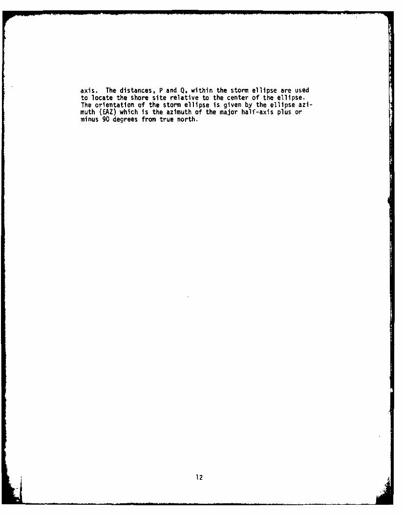
axis. The distances, P and Q, within the storm ellipse are usedto locate the shore site relative to the center of the ellipse.The orientation of the storm ellipse is given by the ellipse azi-muth (EAZ) which is the azimuth of the major half-axis plus orminus 90 degrees from true north.

12

Y N

AA.NoN

0ANG

Storm> Center ..... LAND

>**Site) Shr0

-II

B..:.....:.:: .

Figure 2. A. Map coordinate system (X-Y) for locating storm

center and shore site, and B. Storm coordiante system(Xl-Yl) with origin at storm center and X axis parallelto the shore.

13

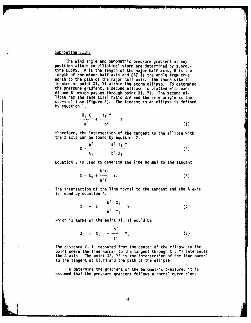
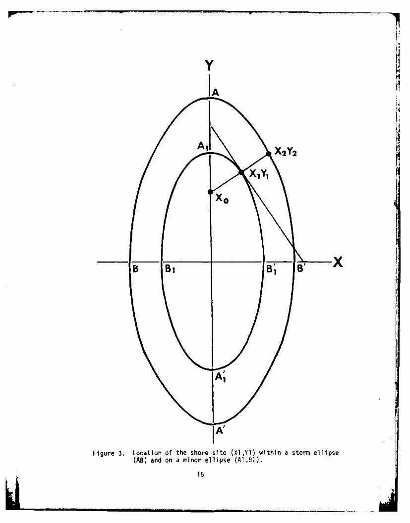
Subroutine ELIPS

The wind angle and barometric pressure gradient at anyposition within an elliptical storm are determined by subrou-tine ELIPS. A is the length of the major half axis, B is thelength of the minor half axis and EAZ is the angle from truenorth to the path of the major half axis. The shore site islocated at point Xl, Yl within the storm ellipse. To determinethe pressure gradient, a second ellipse is plotted with axesAl and Bl which passes through point Xl, Yl. The second el-lipse has the same axial ratio B/A and the same origin as thestorm ellipse (Figure 3). The tangent to an ellipse is definedby equation 1.

X, X Y1 Y+ =

a2 b2 (1)

therefore, the intersection of the tangent to the ellipse with

the X axis can be found by equation 2.

a2 a2 Y, Yx = - - (2)X, b2 X,

Equation 3 is used to generate the line normal to the tangent

b2X1X = X 0 + - Y. (3)

a2y1

The intersection of the line normal to the tangent and the A axisis found by equation 4.

b2 X,xo = x Y (4)

a2 Y1

which is terms of the point Xl, Yl would be

b2

X- = X, YJ (5)a,

The distance X, is measured from the center of the ellipse to thepoint where the line normal to the tangent through Xl, Yl intersectsthe A axis. The point X2, Y2 is the intersection of the line normalto the tangent at Xl,Y1 and the path of the ellipse.

To determine the gradient of the barometric pressure, it isassumed that the pressure gradient follows a normal curve along

14

IA'

Fiue .Loaio fth hoesie(X~)wihn tomelis(AB an o a inr elipe A1,l)

15Y

the major axis of the ellipse. P1 is the barometric pressureat point X0 along the A axis. The pressure at Xo is used indetermining the pressure gradient normal to the isobar at pointXl,Yl. The final pressure gradient calculation is made in sub-routine WIND. XA and YA are used to plot the tangent to theellipse at Xl,Yl for determining the wind direction. The winddirection is assumed to be parallel to the tangent to the el-lipse at Xl,Yl and in a counterclockwise direction around thecenter of the ellipse.

16

Subroutine WIND

The geostrophic wind speed and direction for each stormposition are computed in subroutine WIND. The equation for geo-strophic wind speed V is based on latitude and barometric pres-sure gradient. g

S A P (6Vg- 2 s sin AN (6)

where S is the specific volume, (779 cm3/gm), -6 is the angularvelocity, (7.29 x 10-5 rad./sec.), is the latitude in degrees,and AP/AN is the barometric pressure gradient normal to the iso-bar at the shore location (Godske et al, 1957, p. 370). The baro-metric pressure gradient is computed at right angles to the tan- 4gent of the ellipse through the shore site, (point Xl, Yl). Tocompute the gradient, a normal curve is constructed perpendicularto the tangent through point Xl, Yl. The derivative of the normalcurve is taken at point Xl, Yl to compute the barometric pressuregradient. The geostrophic wind direction is assumed to be parallelto the tangent of the ellipse at point Xl, Yl and heading in a coun-ter-clockwise direction around the center of the ellipse. It isassumed that the small ellipses within the storm ellipse are par-allel to isobars. Therefore, wind direction can be determined ifthe geostrophic wind is directed along the isobars with the highpressure to the right and low pressure to the left of the motionin the northern hemisphere. By means of geostrophic wind equations,the wind direction can be estimated with error of less than 100,and speed with an error of less than 20% (Cole, 1970, p. 185).

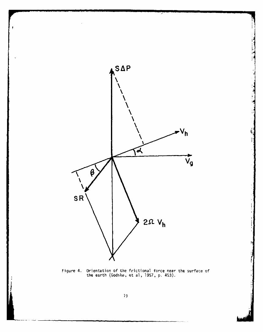
An approxiamte relationship exists between the speed and directionof the surface wind measured at anemometer level and the upper quasi-geostrophic wind. Owing to differences in surface roughness, thisrelationship varies from one station to another, and also varies ata single station with stability. Thus it is rather difficult to de-termine the surface wind accurately from the upper quasi-geostrophicwind. Under average conditions, a rough method may be applied whichmakes use of the horizontal friction force, SR, near the ground(Figure 4). The equation for horizontal motion can be used for com-puting the friction force at a given station (Godske, 1957, p. 453).

sR = Vh + SVhP+ 2,z k x vh (7)

17

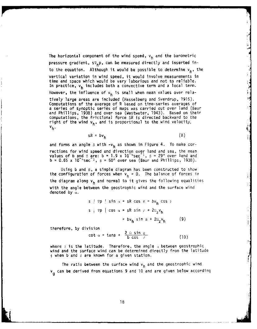
The horizontal component of the wind speed, vh and the barometric

pressure gradient, svhP, can be measured directly and inserted in-

to the equation. Although it would be possible to determine Vh, the

vertical variation in wind speed, it would involve measurements intime and space which would be vary laborious and not to reliable.In practice, vh includes both a convective term and a local term.

However, the influence of vh is small when mean values over rela-

tively large areas are included (Hasselberg and Sverdrup, 1915).Computations of the average of R based on time-series averages ofa series of synoptic series of maps was carried out over land (Baurand Phillips, 1938) and over sea (Westwater, 1943). Based on theircomputations, the frictional force SR is directed backward to theright of the wind vh, and is proportional to the wind velocity,vh,

sR = bvh (8)

and forms an angle B with -vh as shown in Figure 4. To make cor-

rections for wind speed and direction over land and sea, the meanvalues of b and are: b 1.9 x l0-4sec-1, i 290 over land andb = 0.65 x l04sec- 1, = 50' over sea (Baur and Phillips, 1938).

Using b and B, a simple diagram has been constructed to show

the configuration of forces when vh = 0. The balance of forces in

the diagram along vh and normal to it gives the following equalities

with the angle between the geostrophic wind and the surface winddenoted by c.

s vp sin a = sR cos P = bvh cos

s vp I cos o = sR sin f + 2 ,zvh

= bv sin h + 2s2v (9)bh h ~therefore, by division

cot = tana + b sin (

bcos (10)

where . is the latitude. Therefore, the angle . between geostrophicwind and the surface wind can be determined directly from the latitude,t when b and are known for a given station.

The ratio between the surface wind vh and the geostrophic wind

vg can be derived from equations 9 and 10 and are given below according

18

i

SAP

Vh

Vg

SR

2S'LVh

Figure 4. Orientation of the frictional force near the surface ofthe earth (Godske, et al, 1957, p. 453).

19

to Godske et al, 1957.

Vh = vh =s I vpI sina 2s sinVg s Ive b cos 6 s vp

therefore,

Vh _ 2 P sin sin

vg b cos (1l)

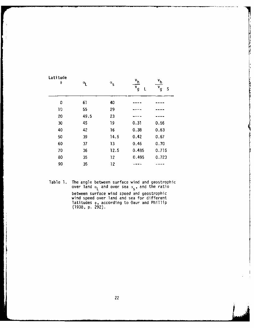
Once the angle c between the surface wind and geostrophic windhas been computed, it can be inserted into equation 11 to computethe ratio between the surface wind and the geostrophic wind overland or sea. Table 1 gives values at different latitudes for ,the angle between surface wind and geostrophic wind, and vh/vg,

which are plotted in Figure 5. In subroutine WIND, the correctionfactors for computing surface wind speed and direction are com-puted following statement 50.

Since the values for b and are given for wind blowing overland or over sea, intermediate values must be computed for windsblowing along the shore. Winds blowing directly onshore with awind angle of zero would have values of b = .000065 and = 50.In this case, the wind is blowing from the sea and the land doesnot have any frictional effect on the wind. In like manner, ifthe wind is blowing over the land in an offshore direction, valuesfor the land, b =.000190 and = 20 are applied. FQr the transi-tion zones, a cosine transformation is used to compute the inter-mediate values. Within the transition zone, angle A is computedfrom 0 to 90' with 0 being land and 900 being sea. The new angleA is used in equations 12 and 13 to compute the transition valuesfor b and beta.

b =.0001 • (1.275 + .625 (sin A)) (12)

39.5 - 10.5 • sin A (13)

The computed values for b and are substituted in equations 10 and11 to compute the surface wind speed and direction from the geo-strophic wind.

The final step in subroutine WIND is to compute the effectivewind speed which is carried over into subroutines FETCH and WAVESfor determining effective fetch length and wave height. The effec-

20

tive wind speed is that which will generate waves which will in turnhave an effect on the beach. If the wind is blowing directly on-shore, the full force of the wind is used in generating waves whichwill hit the coast. However, if the wind is blowing directly off-shore, small waves will be generated in the nearshore area (Resioand Hayden, 1973). Based on empirical observations, onshore windsare about three times as effective in generating local waves asoffshore wind (Davis and Fox, 1974 and Owens, 1975). Therefore,

fective wind speed from the surface wind speed and direction.

When the wind is blowing directly onshore, the effective wind isequal to the surface wind. On the other hand, when the wind is14blowing along the shore, the effective wind is equal to 2/3 ofthe surface wind, and when the surface wind is blowing directlyoffshore, the effective wind is 1/3 the surface wind. Althoughthe values for effective wind may be rough in some cases, theyseem to give good estimates where comparative wind and wave dataare available.

21

Latitude V V

L sh hV Vg L gS

0 61 40 ---- ----

10 55 29

20 49.5 23 ---- ----

30 45 19 0.31 0.56

40 42 16 0.38 0.63

50 39 14.5 0.42 0.67

60 37 13 0.46 0.70

70 36 12.5 0.485 0.715

80 35 12 0.495 0.723

90 35 12

Table 1. The angle between surface wind and geostrophicover land aL and over sea as , and the ratio

between surface wind speed and geostrophicwind speed over land and sea for differentlatitudes , according to -Baur and Phillip(1938, p. 292).

22

hi60,

ZF

W 20-SEA

W 0

010 20 30 40 5 60 70'i 8 0 9 0LATITUDE (0)

00*00 SEA.61e

0 4

Im .5-'4

C1 0

0

CO rt .3-

.23

Subroutine DECAY

Subroutine DECAY is used to determine the height of a givenwave after it has decayed for a specified length of time. Snod-grass, et al (1966) presented empirical data on the attenuationof selected frequencies which they observed in their study ofpropagation of ocean swell in the Pacific. In general, theyfound the attenuation to be large within the limits of the windarea of the storm, and small outside the storm area. The em-pirical attenuation data were logarithmic coefficients reportedin units of decibels per latitude degree of propagation distance.For the range of frequencies 0.06 to 0.08 Hertz, these data fitan attenuation function of the form

e-2ax (14)

-Iwhere a is the modulus of amplitude decay in degree- 0.1151 ~where is the logarithmic attenuation coefficient in decibels/degree, and where x is the propagation distance in degrees.The logarithmic attenuation coefficient versus frequency wasplotted on a graph (Kaufman, 1973), and equation (15) was de-rived from the line on the graph.

( -0.06~=0 034(15)

where F is the frequency of the wave being decayed.

The propagation distance x is found by multiplying the wavevelocity l.5606*T (where T is the wave period) times the timeinterval TINT. This distance is then reduced to degrees bymultiplying it by the constant value

360'/circle40074Wm/circ e

(using the circumference of the earth at the equator). To findthe decayed wave height then, the original wave height is miulti-plied by the attenuation function. This decay factor was testedwith several different wave heights, periods, and time intervals,giving very reasonable decay results, but there were no empirical

data against which to check the results.

24

Subroutine ETIME

Subroutine ETIME is used to determine the amount of time(referred to as effective duration) which would be required toproduce waves of a certain height by wind blowing at a given windspeed. A wave forecasting procedure developed by Sverdrup andMunk (1947), and revised by Bretschneider (1952, 1958) with ad-ditional empirical data is called the sverdrup-Munk-Bretschenider(SMB) method (C.E.R.C., 1973). The SMB curves for forecastingwave height are based on equation 16 from Bretschneider (1958).

-UM 0.283 Tanh [ 0.0125 IF ) 16

where g is the acceleration due to gravity, H is the wave height,F is the effective fetch length, and U is the wind speed. Solvingequation 16 for F gives

_U2 ARCTANH( H.83 U-)

xL 0.012 (17)

Therefore, F is the effective fetch that it would take to generatewaves of height H with a wind speed of U.

In terms of storm duration, the effective fetch equation is

F - S 0.72 00.3 )D.2510 x 1 D1 18

Where F is effective fetch, W is wind speed, and D is storm duration.Solving this for D, we have:

( F 0.8D= S 0.72 0

I0 x 10 " (19)

Therefore, D is the effective duration that it would take to buildwaves of a certain height (used to find the effective fetch) withwinds of a given speed. Then, this effective duration isadded to the current time increment of the storm to give a durationwhich takes into account the wave built in previous time increments.

Subroutine ETIME was tested by running the data from subroutineWAVES back through it to arrive at the original data. For example,

25

the following wave heights and wind speeds were tested usingthe C.E.R.C. charts and the subroutine (Table 2).

Effective Duration

Wave Height Wind Speed From SMB Curves Derived

14 ft 80 kts 1.1 hrs 1.05 hrs

1 ft 12 kts 1.4 hrs 1.38 hrs

45 ft 80 kts 9.9 hrs 10.23 hrs

3 ft 12 kts 21.0 hrs 21.40 hrs

14 ft 30 kts 21.0 hrs 21.76 hrs

Table 2. Test for subroutine ETIME comparing effectiveduration available from SMB curves with derivedduration for selected wave heights and windspeeds.

26

Subroutine FETCH

Subroutine FETCH is used to determine the maximum wind gen-erating area and the average wind speed within that area for acircular storm on the open ocean. Three cases are considered fordetermining the actual storm fetch as the storm passes across ashoreline.

For a storm on the open ocean, the wind speed varies withthe slope (first derivative) of a normal curve as one crossesthe storm. The area of the storm with wind speed greater thanone half of the maximum lies within a ring with an outside radiusof 1.92 standard deviations and an inner radius of 0.32 standarddeviations. This ring between 1.90 and 0.30 was divided into 13smaller rings. The area of each ring was found and multipliedby the wind speed at the midpoint of the ring. These products weresummied and then divided by the total area to give an average windspeed of 0.8847 of the maximum wind speeu. The total area wasfound to be 7.7598 square standard deviations. Since the wind isbeing generated in a circular pattern, approximately one quarterof the wind is blowing along each axis of a grid with its centerat the origin. Since the storm fetch area has a shape resemblingan ellipse, the fetch for winds blowing in any one direction canbe considered an ellipse with an area equal to one quarter of themaximum wind generating area (1.9400 square standard deviations)and centered on the maximum wind speed circle (1 standard devi-ations). The short half diameter was taken to be 0.7 standarddeviations (1.0-0.3).

Area 7x ax b

1.9400 =3.1415 x a x .7

a =0.8822 standard deviations (20)

Therefore, the maximum storm fetch length Is twice that, or 1.7644standard deviations. Converting to storm radii, the fetch is 0.5881radii.

Where the storm crosses the shoreline three cases must be con-sidered; Case 1, where 1/3 R -x > 0; Case 2, where 0.4444 R -x > 1/3R and Case 3, where x > 0.4444 R, where R is the storm radius and xis the distance from the center of the storm.

For Case 1, (1/3 R > x >0) (Figure 6), it is assumed that thefetch area, centered on the T/3 R circle, swings around so that thelong axis of the ellipse is always pointing at the beach. We havemaximum storm fetch in this case until Y is small enough that thefetch begins to cross the beach as it continues to swing. Thispoint is Y1. From the Case One diagram, D2 X2 + YV and D-

27

(1/3 R) 2 + (1/2 F) 2 so we have X2 + Y]b' (1/3 R)" + (1/2 F) 2 or

Y= (1/3 R)2 + (1/2 F)2 - X2 (21)

As the storm continues to cross the beach and rotate, the fetchdecreases. When the 1/3 R circle of the storm crosses the beach,the storm has swung so that the beach is in the center of the fetcharea. Therefore, the storm fetch is one half of maximum at thispoint (Y2). As the storm continues inland, the fetch length reachesa minimum as Y goes to zero (Y3). This minimum is determined bythe equation 22.

I X I

FMIN = FMAX. (22)

This gives a diminishing minimum as jx' goes to zero. The fetchthen increases to a high equal to 1/2-FMAX as the 1/3 R circle a-gain crosses the beach (Y4). The fetch then declines again, fin-ally dropping to zero at Y4, at which point the storm is completelyonshore. This gives the "eye of the storm" effect where the windsdrop to a minimum when the storm is at its closet point of approachand then increase again as the storm moves on, and finally drop asthe storm moves away. Cosine smoothing is used to smooth out theincreases and decreases in fetch.

For Case 2 (0.4444 R - x > 1/3 R)(Figure 7), again we have fullfetch until the fetch area comes into contact with the beach at Yl.The fetch then decreases as the storm moves onshore, hitting zeroat Y2. The reason that the fetch doesn't drop and then rise again,as in Case One, is that the eye of the storm (the part inside the1/3 R circle) never passes over the beach.

This case ends at X = 0.4444 R because D in the case two dia-gram = V'(1/2 R)&'+ (1/2 F)2 = 0.4444 R. When X D, then the geo-metric relationships that allow us to find Yl no longer hold, since0, the distance from the origin to the beach, can no longer equalboth A2 + Yl and (/3 R) + (1/2 F)". Again consine curvesare used to smooth out the changes in storm fetch.

For Case 3, ( x .0.4444 R)(Figure 8) the storm fetch area neveractually crosses the beach, but the fetch decreases as the storm pas-ses over the shore farther along the coast. Thus the storm fetch isat its maximum until the fetch area starts going onshore at Yl. Herethe fetch is perpendicular to the storm path. Yl is at zero sinceat that point, the whole half of the storm that is generating along-shore waves is still over the water, so we still have full fetch.As the entire storm passes onshore (Y2), the fetch drops to zero.Y2 Is -v/" - (0.4444R) . Y2 is frozen, using an X value of 0.4444R.

28

Y1.

Y, A

Ys- a jfT/ x' W

Figure 6. Case 1 - storm fetch when the distance from center of s~tormnX is less than 1/3 storm radius, R.

290

Ar

Y, '

Figure 7. Case 2 - stormo fetch when the distance from center of stormX is less than 0.4444 and qreater than 1/3 storm radius, P.

30

ye y4

x

0i~. 14 Y * 1

Figure 8. Case 3 -storm~ fetch when the distance from center of storm

X is qreater than 0.4444 storm radius, R.

31

The reason that this is valid, is that from X =0.4444 R on out,the fetch area never actually passes over the beach, so that allthese cases are essentially the same, as far as the size of theirstorm fetches goes. Only the distance from the storm fetch tothe beach changes.

Subroutine FETCH was tested in two ways. First X and Y werevaried independently, running Y from +R to -R for each value of X.This simulated storms with paths perpendicular to the shoreline.Second, X and Y were varied simultaneously by a constant amount,simulating storms crossing the shoreline at an angle. In bothcases, the program produced continuous curves of fetch varying withstorm location, with smooth transitions between all cases.

32

Subroutine WAVES

The equations for predicting significant wave height andperiod in subroutine WAVES are based on the Sverdrup-Munk-Bretschneider (SMB) method revised by Bretschneider (1958)and plotted as a series of curves by C.E.R.C. (1973). The SMBwave forecasting curves for fetches of I to 1000 miles are givenin Figure 9. The wave prediction curves use the wind speed inknots, storm duration in hours, and storm fetch to calculate thesignificant wave height and significant wave period.

In order to use the SMB method in the model, the first taskwas to find equations to approximate the effective fetch from thewave prediction curves. The effective fetch is the limiting fetchwhich corresponds to a given wind speed and duration. The effect-ive fetch is determined by moving to the left across the chart atthe level of the wind speed until you hit the appropriated stormduration line. Then drop straight down to the fetch length axisfrom the intersection of the wind speed line with the durationline. This value on the fetch length axis is the effective fetch,if it is less than the actual fetch.

To develop an equation for effective fetch, the first problemis to determine the intercept of the proper duration line. To dothis, the intercept of each line with the fetch length axis wasplotted against the storm duration. Log scales were used on bothaxes since the original fetch length axis had a log scale and theduration lines themselves were spaced logarithmically. Theseformed a nearly linear trend and the equation for the line wasfound, in terms of the log axes, to be:

I = 10 0.3 XD o1.25 (23)

where I is the intercept and 0 is the storm duration.

The next step was to determine the slope of the storm duration

lines given in the following equation.

0.7F(10) x I (24)

where F is the effective fetch, S is the wind speed, and I is theintercept of the duration line with the fetch length line. Coin-bining equations 23 and 24 we get equation 25 for the effectivefetch in terms of wind speed and storm duration:

F ( .2x (10 0.3 x D01.25) (25)

33

If this value is less than the actual storm fetch then it decreasesthe relevant fetch length which is used in the rest of the equations.

The SMB forecasting curves were constructed from equations 26and 27, which were empirically derived by Bretschneider (1958).

= 0.283 TANH ( 0.025(F)°' ) (26)

9T = 1.20 TANH 0.077( U )) (27)2pU

where g is the gravitational constant, p is PI (3.1459), H isthe significant wave height, U is the wind speed, F is the effectivefetch, and T is the significant wave period. Solving these equationsfor H and T, we get equations 28 and 29.

U2 x 0.283 x TANH( 0.125(J) )H= (28)g

T T 2pU x 1.20 x T)NH () °77 (29)g

The values for wind speed, storm duration, and effective fetch arethen inserted into equations 28 and 29 to yield the wave height andperiod. For example in the case of a storm with a duration of 10hours, a wind speed of 35 knots, and an actual fetch of 200 nauticalmiles, this gives us an effective fetch of 87.44 nautical miles, awave height of 12.78 feet, and a wave period of 7.85 seconds. Butsuppose that we have a storm the same as the last one, but with afetch of only 80 nautical miles. In this case the actual fetch issmaller than the computed fetch, so it remains as the effectivefetch. This gives us a wave height of 12.36 feet and a wave periodof 7.72 seconds.

The program has an option so that the results can either bemetric or, to facilitate checking the results against the SMB curves,the results can be in nautical miles and feet. The subprogram wastested with numerous combinations of wind speeds, durations, andfetch lengths, with the results agreeing very well with the SMBforecasting curves.

34

! ...

Al"O 1*d ge.. 1 4dS I...

V .8

z 06 2

/T t

Or 7r

.... . .

Figure 9. Deepwater wave forecasting curves as a function of windspeed, fetch length and wind druation based on the S.M.B.method.

35

Subroutine TIDE

Subroutine TIDE is used to determine the tide level at eachhour, the spring tide range (ST), the neap tide range (NT), thenumber of days since the last spring high tide (TDAY), the hourof the last high spring tide (THR), and the tidal form number(FN). Four principal tidal components, M2 - Principal lunar,

S2 - Principal solar, K1 - Lunar-solar diurnal, and 01 Prin-

cipal lunar diurnal are used for making a prediction of the hourlytide level. The periods of the semi-diurnal components (TM212.42 hours and TS2 = 12.00 hours) and the diurnal components(TKI = 23.93 hours and TOl = 25.82 hours) are constants in thesubroutine. The tidal form number FN is used to classify thetides of a locality according to equation 30 (Defant, 1960, p.306). F+

K1 + 0

FN = M2 + $2 (30)

The following classification based on Dietrich (1944, p. 69) isused to classify tides according to their form number.

FN = 0 - 0.25 Semi-diurnal tide

FN = 0.25 - 1.50 Mixed- mainly semi-diurnal tide

FN = 1.50 - 3.00 Mixed- mainly diurnal tide

FN = greater than 3.0 Diurnal tide

As examples of the different types of tides, Immingham, Englandhas a semi-diurnal tide with a form number of 0.11. San Francisco,California has a mixed, dominately semi-diurnal tide with a formnumber of 0.90. Manila has a mixed, dominately diurnal tide with aform number of 2.15, and Do San, Viet Nam on the Gulf of Tonkin hasa pronounced diurnal tide with a form number of 19.2. The four ma-jor components are responsible for the general form of the tidesand generallyaccount for about 70 percent of the total variance.If the next three most important tidal components, N2, K2 and P1

are included, the percentage of the total variance increases toabout 83% (Defant, 1960).

If some simplifying assumptions are made concerning the majortidal components, it is possible to make a good approximation ofthe hourly tide level from the maximum spring tide range, minimumneap tide range, and the tidal form number. First, it is necessaryto assume that the diurnal components, K1 and 01 are approximately

equal. Second, assume that the maximum spring tide range is equal

36

r2

to the sum of the four major components according to equation 31.

ST = M2 + S2 - (K1 + 01) (31)

Next it is assumed that the neap tide range is approximately equalto the lunar components minus the solar components.

TN = M2 + K1 - (S2 + 01 ) (32)

If K1 and 01 are approximately equal, it follows that

TN = M - S2 (33)

The form number is the diurnal components over the semidiurnalcomponents in equation 30, however, if K1 = 0l' then

FN K,2 K(M2+ S2

By combining the equations for the.form number (Equation 30),the spring tide range,and the neap tide range, it is possible tosolve for M, and S2 .

- ST + TN (35)

M 4 (l + FN)

and

ST - TN (36)$2 = 4 (I-FN)

If it is now assumed the lunar components are proportional,

an approximation of the K1 component can be derived from the M2

component

K1 = FN • M2 (37)

and the solar components are related in like manner, therefore,

01 = FN • S2 (38)

The amplitude of the maximum spring tide was taken at the lastprevious spring tide for each run, therefore, the phases for the fourmajor components are considered 0 at that time. By computing thetime differences from the last spring high tide to the hour for theprediction, the contribution for each tidal componcnt can be calcu-lated. The argument (ARG) is equal to 2 pi times the number of hourssince the last spring tide. The tide is computed by adding togetherthe contribution for each of the tidal components.

37

2 ( ARG )+ S2 SARG

TM22K cosAR + 0ARG

Kl 1 * °l cosV (39)

Although some rough approximations were made in deriving themajor tidal components from the spring tide range, neap tide rangeand form number, the resulting tide predictions work out quiteclosely with the tide tables. The tide tables give the time ofhigh and low tides for each day, and the predicted times of highand low tides fall within I hour using subroutine TIDE. The sub-routine was tested for Plum Island, Massachusetts, Cedar Island,Virginia, Sapelo Island, Georgia and Mustang Island, Texas, andgave satisfactory predictions for each of the areas.

One of the major reasons for making tidal predictions in themodel is to determine the effect that tides have on the nearshorebottom slope. The slope at low tide SLBOT, the slope at high tideSLTOP and the tide level are used to determine the intermediateslope between high and low tide.

SLOPE = SLBOT + TLOC *(SLOTP - SLBOT) (40)

The final tide level which is included with the output iscomputed by adding the relative tide level TIDX to the mean lowtide level TMEAN.

38

Subroutine SURF

Breaker height, angle and longshore current velocity arecomputed in Subroutine SURF. The critical value, Hb/hb = .78

where Hb and hb are breaker height and depth, are used for a

breaking criterion (Munk, 1949). Applying any wave theory andassuming conservation of energy flux, Komar and Gaughan (1972)derived the relationship

Hb = 0.73 cm + .383 g1/5 (T H2 )2/5 (41)

where Hb is the breaker height, g is gravity, T is wave period

and H_ is the deep water wave height.

The breaker angle ab is computed by first finding the shallow

water wave length and then taking the ratio of shallow water todeep water wave length using Snell's law to determine the breakerangle.

sin b sin a0 TANH(27Hb ) (42)

where is the deep water wave angle which is assumed to be the

same as the wind angle, Hb is the breaker height and Lb is the

breaker depth.

The refracted breaker height, HR, is obtained from the re-fraction coefficient, KR,

cos (U0 )KR - cos (ab) (43)

which is multiplied times the breaker height, Hb

HR = KR 0 Hb (44)

Four different options are available for computing the long-shore current velocity. The longshore current equations by Longuet-Higgins (1970), Komar and Inman (1970), Fox and Davis (1972) andCoastal Engineering Research Center (C.E.R.C., 1973) used basicdifferent assumptions with the same set of variables. The variation

39

in longshore current velocity across the surf zone and along theshore, as well as differences in nearshore topography brought aboutby bars and rip channels make any prediction of average longshorecurrent velocity very difficult. However, in making predictionsabout the surf zone, it is essential to at least have a good esti-mate of the maximum longshore current velocity.

The radiation stress theory of Longuet-Higgins (1970) hasbeen tested with laboratory data from Galvin and Eagleson (1965),and field data from Putman, Munk and Traylor (1949). The long-shore current velocity in the surf zone, Vb, is a function of thebottom slope, m, the breaker height, Hb, and breaker angle, d1b' 1between the wave crest and the shoreline (Longuet-Higgins, 1970).

Vb = Mlm (gHb) sin 2ab (45) 4where Ml, the friction factor is:

= 0.694 r (2)-1/2M l -ff(46)

ff

The longshore current, Vb is measured at the breaking position and

r is a mixing coefficient with a range of 0.17 (little mixing) to0.5 (complete mixing) with a mode at about 0.2. The depth toheight ratio in shallow waver, 3, is taken to be 1.2 and ff the

friction coefficient is set at 0.01. By inserting the above valuesin equation 46, the value for M1 becomes 9.0. Therefore, the long-

shore current equation according to Longuet-Higgins (1970) can bereduced to:

Vb = 9.0 m (gHb) 1/2 sin 2 b (47)

When equation 47 was applied to test sets of field and lab-oratory data by C.E.R.C. (1973), the data yields predictions thataverage about 0.43 of the measured values. The measured valueswere taken in the fastest field of flow shoreward of the breakerzone, whereas the predictions were made for longshore current atthe line of breakers. Therefore, it has been proposed by C.E.R.C.(1973) that the Longuet-Higgins equation be multiplied by 2.3 toyeild the C.E.R.C. equation:

V = 20.7 m (gHb)l/2 sin 2.,b (48)

40

Komar and Inman (1970) derived a longshore current equationbased on radiation stress. Where the radiation stress componentsdefined by Longuet-Higgins and Stewart (1964) is the excess flowof momentum due to the presence of waves. The Komar and Inman(1970) equation is:

V=CU Tan sin )cos1 m Cf 'b co 4b

where V is the longshore current velocity, Tan is the beachslope, Cf is the bottom frictional drag coefficient. Um is the

maximum horizontal component of the orbital velocity of the wavesand C1 is a dimensional coefficient of proportionality. However,

Komar (1969) suggested that: 4

(Tan 1 cos ab)/Cf = constant (50)

indicating that the variation in beach slope does not produce achange in longshore current velocity. Therefore, the Komar andInman (1970) longshore current equation becomes:

V = ClUm sin (51)

A fourth equation developed by Fox and Davis (1972) uses em-pirical data subjected to linear regression analysis to predictlongshore current velocity. The linear regression analysis isbased on 3 sets of data collected at Stevensville, Michigan (Foxand Davis, 1970), Holland, Michigan (Fox and Davis, 1971a) andSheboygan, Wisconsin (Fox and Davis, 1972). Each set of dataconsists of 360 observations taken at 2 hour intervals for 30 daysof longshore current speed and direction, breaker height, periodand breaker angle. Using a stepwise regression analysis, the con-tribution of each variable was tested separately, and then in var-ious combinations. The ratio, Hb/T is related to the mass flux on

volume of water which enters the surf zone and must be removed bythe longshore current. The breaker angle, ab, defines the anglebetween the breaker crest and the shoreline and is therefore re-lated to the momentum transfer in the longshore direction. Usingthe regression program, a series of combinations was tested forthe sin of the angle including sin A, sin 2A, sin 3A, sin 4A...sin 8A. The closest fit was obtained when sin 4A was used for theangles. For the 1969 set of data from Stevensville, Michigan, thefollowing equation,

41

V 5.42 Tb sin 4A (52)

gave the best fit and accounted for 83.5 percent of the total sumof squares. For the 1970 data from Holland, Michigan, the coef-ficient of proportionality was 3.47 and the equation accounted for78.8 percent of the total sum of squares. For the 1972 data fromSheboygan, Wisconsin, the coefficient was 2.98 and the equationaccounted for 77.8 percent of the total sum of squares.

The three areas differed in the nearshore bottom slope andthe occurrence of sand bars which influenced the coefficient ofproportionality. The coefficient for each case was approximatelyequal to 100 times the bottom slope. Therefore, the longshorecurrent velocity according to Fox and Davis (1973) is

V = 100 m( b sin 4 x b (53)

When the four longshore current equations were tested in themodel, the equation by Longuet-Higgins (1970) and Fox and Davis(1973) gave very similar results for breaker angles up to about20 degrees. For higher breaker angles, the predicted results fromthe Fox and Davis (1973a) equation were too low. The values forlongshore current predicted by Komar and Inman (1970) and C.E.R.C.(1973) were consistantly too high. Although the four equations areavailable as options, it is recommended that the Longuet-Higgins(1970) equation be used for making predictions. If possible, itis best to test predictions with hindcast data from the same area.

42

Subroutine ENRGY

Subroutine ENRGY is used to determine the wave energy duringeach hour of the storm which is summed to give the total waveenergy for the storm. The deep water wave energy E. (C.E.R.C.,1973) is given by

E p g HL 5.12 g (HL) (54)o 8 8

where , is the mass density of the water which is 1.94 slugs/cubicfoot for fresh water and 2.0 slugs/cubic foot for salt water, H isthe deep water wave height and T is the wave period. Conversionfactors are included to change from foot pounds/foot to Joules/meter. The subroutine was tested using wave energy calculationfrom previous studies (Fox and Davis, 1971b).

Subroutine ARCTA

Subroutine ARCTA is a customized arctangent subroutine forfinding the angle in radians from the arctangent of a function(Louden, 1967, p. 119). The library arctangent function ATANaccepts as an argument the tangent of an angle (sin/cos) and pro-duces as output the angle in radians. Since the tangent of anangle repeats itself every 180 degrees, it is not possible touse the library function ATAN to determine a full range of anglesfrom 0 to 360 degrees. To compute the correct angle for all pos-sible combinations of X and Y, it is necessary to test for positive,near zero and negative X, and positive near zero and negative Y.The IF statements accomplish these test and produce an angle inradians ranging from 0 to 2 pi.

43

HINDCAST ANALYSIS WITH COASTAL STORM MODEL

Hindcast Tests of Model

The coastal storm simulation model can be used to hindcastwind, wave and current conditions at a shore site during thepassage of a coastal storm. Hindcast analysis differs fromforecast analysis discussed in the previous section becauseexact storm positions are known in hindcasting, whereas a con-stant azimuth and storm velocity are used in forecasting. Tteresults of hindcast analysis at several sites are included inAppendix C. On the Great Lakes, the sites include Holland andStevensville, Michigan, and Sheboygan, Wisconsin. On the eastcoast of the United States and Canada, sites include the Mag-dalen Islands on the Gulf of Saint Lawrence; Plum Island, Mass-achusetts; Cedar Island, Virginia and Sapelo Island, Georgid.Mustang Island, Texas was studied on the Gulf Coast. (n thewest coast of the United States, hindcasts were made for Mon-terey, California and South Beach, Oregon.

Sites were selected for hindcast analysis which had weatherand wave data available for several storms. Several of the siteswere studied by Davis and Fox using time series analysis from 1969through 1975. Other sites were chosen in which there was good beachprofile data which could be correlated with wave and current condi-tions during a storm.

Stevensville, Michigan, July 1969

A storm which passed over Lake Michigan in late July 1969has been choosen as an example of hindcast analysis. When thestorm passed over, a 30 day time-series study was being conductedat Stevensville, Michigan by Fox and Davis (1970a and b). Stevens-ville is located on the southeastern shore of Lake Michigan about11 kilometers south of Benton Harbor, Michigan. The shoreline isoriented roughly north-south with an average nearshore slope ofabout 0.033.

The storm which affected the Stevensville area was trackedfrom 2000 on July 26, 1969 through 0800 on July 30 (Table 3).The size, shape, intensity and path of the storm were interpretedfrom weather maps for July 26 through 30, 1969. When the stormwas closest to the coastal site at Stevensville, the barometricpressure at the center of the low was estimated as 994 millibars.The pressure at the largest encircling isobar was 1012 millibars,and therefore, the maximum pressure included in the storm was 1014.6millibars. The storm had an elliptical shape with the length ofthe major half axis equal to 960 kilometers and the minor half axis

44

-'A.

* p A9

A * A - - . - ..........

- . . . . . p

.7

equal to 700 kilometers. The orientation of the major half axiswas 30 degrees west of north. For this particular example, theequation by Fox and Davis (1972) was used to compute the long-shore current velocity.

The position of the shoreline at Stevensville is given inthe X-Y coordinate system with X equal to 1043 and Y equal to 486kilometers. The X axis runs east-west and the Y axis north-southwith the origin located to the southeast of Stevensville. Thelatitude at the shore location is 420 north and the onshore azi-muth is 90 degrees. The nearshore slope from the shoreline outacross the nearshore bars is 0.033. The average fetch distancefor the southeastern shore of Lake Michigan is about 200 kilo-meters.

The storm positions were plotted at 6 hour intervals in kilo-meters on the X-Y coordinate system (Table 3). The initial posi-tion of the storm at 2000 on July 26 was to the northwest of theshore site with X equal to 333 and Y equal to 1229 kilometers.The storm passed over the shoreline about 0230 on July 28. Atthat time, the storm center was located 178 kilometers north ofthe shore site (664-486 =178 kilometers). When the storm track-ing was complete, the final storm position at 0800 on July 30 wasX equal to 1907 and Y equal to 1830 kilometers. In general, thestorm made a loop swinging down from the northwest, passing east-ward across the shore, then moving off to the northeast.

The Xl, Yl coordinate is oriented with the Xl axis parallel tothe shore and the Yl axis normal to the coast (Figure 2). Theorigin of the Xl, Yl coordinate system is at the center of the stormwith the positive Xl direction to the right and the positive YIdirection toward the coast. The Xl, Yl coordinate system is usedto locate the shore position with reference to the center of thestorm. The units of the Xl, Yl coordinate system are in terms ofstorm radii. The storm radius is 1.5 times the length of themajor half axis which is measured from the center of the stormto the largest encircling isobar. Using an inverted normal curveto simulate the storm cross-section the largest encircling isobaris defined as 2 standard deviations from the center of the storm.The full radius would extend out 3 standard deviations from thecenter of the low. As the storm approaches shoreline, the Yl valuedecreases, and it becomes negative after the storm has passed overthe coast. When the storm is to the north of shore site the Xlvalues are positive. Therefore, the storm at Stevensville remainedto the north of the shore site for the entire run.

In the hindcast analysis, the barometric pressure decreasesfrom 1012.4 millibars on July 26 to a minimum of 995.2 at 2200 onJuly 27, then increased to 1014.6 on July 30, 1969 (Table 3 andFigure 10). In the actual barometric pressure record at Stevens-ville, the pressure dropped to 1000.2 millibars (29.54 inches) at

46

STEVENSVILLE, MICHIGANJULY 25, 1969

,,.7-27..i 7-28,. .7-29 . ,7.-99 1

30.00. BAROMETRIC PRESSURE 1016

29.90" , /,, I11

29.80 1008

:29.70. ="o .1004

S 29.60 "00/,,, / .1000

29.50" ,

29.40 .996

29.30 992

301 WIND VELOCITYLI.d2o , -_. .." 3

0. .0

7 LONGSHORE 210

6 CURRENT .180

5. -150

4 120

3 /90

2- -I60

-30

-2 --60

-3 "-90

-4 -1202.0

6' BREAKER

5. HEIGHT "1.5

4.41.0

32 .0.5

0- 0

Figure 10. Observed and hindcast curves for barometric pressure, windvelocity, longshore current and breaker heicht at Stevens,ville, Michigan, July 26-30, 1969.

* 47

2000 on July 27. Since small scale weather maps were used fordetermining the storm position and pressure values, more accurateresults could be obtained by using large scale maps available at3 hour intervals. The plot for barometric pressure is a functionof accurate plotting of the storm positions and a careful estimateof the size and intensity of the storm. Therefore, a correspondenceof the observed and hindcast curves for barometric pressure is nota test of the predictive capabilities of the model, but is more atest of the accuracy of the weather maps and of the plotting abil-

ity of the operator.

In the wind observations at Stevensville, the maximum windspeed during the storm was 12.4 meters/second (28.4 knots) at 1600on July 28 (Fox and Davis, 1970a). For the hindcast, the maximumwind speed was 12.0 meters/second at 1400 on July 28. The overallpattern for the observed and hindcast winds are also quite similar(Figure 10).

The observed longshore current velocity at Stevensville reached-116 centimeters/second (northerly) at 2200 on July 27, and 215 centi-meters/second (southerly) at 1800 on July 28 (Fox and Davis, 1970a).The maximum hindcast values were -62.9 centimeters/second at 2100 onJuly 2! and 101.9 centimeters/second at 1700 on July 28 (Figure 10and Table 3). The instantaneous longshore current values were muchhigher in the observed than the hindcast values, however, the minimumand maximum values occurred within one hour of the hindcast values.The observed longshore current during the storm was exceptionallyhigh and may be accounted for by the well developed trough betweenthe nearshore bar and the shore which channeled the current alongthe coast. The value used for nearshore slope could also be toolow in the hindcast. When the longshore current curve was smoothedusing the 15 term Fourier plot, the hindcast more closely resemblesthe observed curve for longshore current (Fox and Davis, 1970a andb).

The observed and hindcast curves for breaker height are veryclose (Figure 10). For the observed curve, the maximum breakerhieght of 1.82 meters (6 feet) occurred at 1800 on July 28. Forthe hindcast, the maximum height was 1.83 meters, also at 1800 onJuly 28. The overall shapes of the observed and hindcast curvesfor breaker height are also very similar but the hindcast curvedrops off more rapidly than the observed curve (Figure 10).

48

Additional Hindcast Examples

Additional examples of the hindcast tests are presented inAppendix B and Figures 26, 27, 28 and 29. Since the input para-meters are given in Appendix B ad comparative plots are in Figure26 through 29, a full discussion will not be included for each ofthe examples.

The observed data for the Holland, Michigan examples was ex-tracted from a 30-day time series study during July 1970 (Fox andDavis, 1971a). Holland is located on the southeastern shore ofLake Michigan about 96 kilometers north of Stevensville. The hind-cast values for longshore current and breaker height were quiteclose for July 3, 1970 (Figure 11), but were somewhat low for July18, 1970 (Figure 12).

The observed data for the Sheboygan, Wisconsin examples comefrom a 30-day time series study conducted at Sheboygan during July1972 (Fox and Davis, 1973a). Sheboygan is located on the westernshore of Lake Michigan about 72 kilometers north of Milwaukee,Wisconsin. At this location, the storms moved in a northeast di-rection and generally offshore. Therefore, the characteristic re-versal of longshore current direction observed on the eastern shoreof Lake Michigan was not observed at Sheboygan. The curves for July16 show generally low observed and hindcast curves for longshorecurrent and breaker height with pronounced peaks on July 17, 1972(Figure 13). The curves for July 22 show a substantial drop inbarometric pressure, but very low values for longshore current andbreaker height (Figure 14). There is a reversal in longshore cur-rent direction on July 24 for both the observed and hindcast curves.Since the winds were blowing predominately offshore, the waves andlongshore currents are quite subdued.

Several additional tables of hindcast results are given inAppendix B. The output for the Atlantic, the Gulf and the Pacificcoasts of the United States includes a variety of conditions forstorms of varying sizes, shapes and intensities. Tidal predictionsare also included for the oceanic sites where the tide tables areavailable. Some of the hindcast results followed quite closelywith the observed data, while at other places, the fit was not asgood is expected.

49

*

LAk ,..J

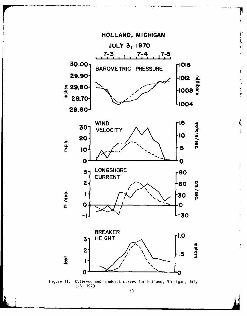
HOLLAND, MICHIGAN

JULY 39 1970T-3 7-4 7-5

30.00 BAROMETRIC PRESSURE 1016

29.90 11

.C lee1008

29.To % 100429.60j

30" WIND IS 4

100

0 00

3. LONGSHORE 90CURRENT

2- 60

1 -30 C

-0

BREAKER 1.0

2-O

Figure 11. Observed and hindcast curves for Holland, Michigan, July3-5, 1970.

50

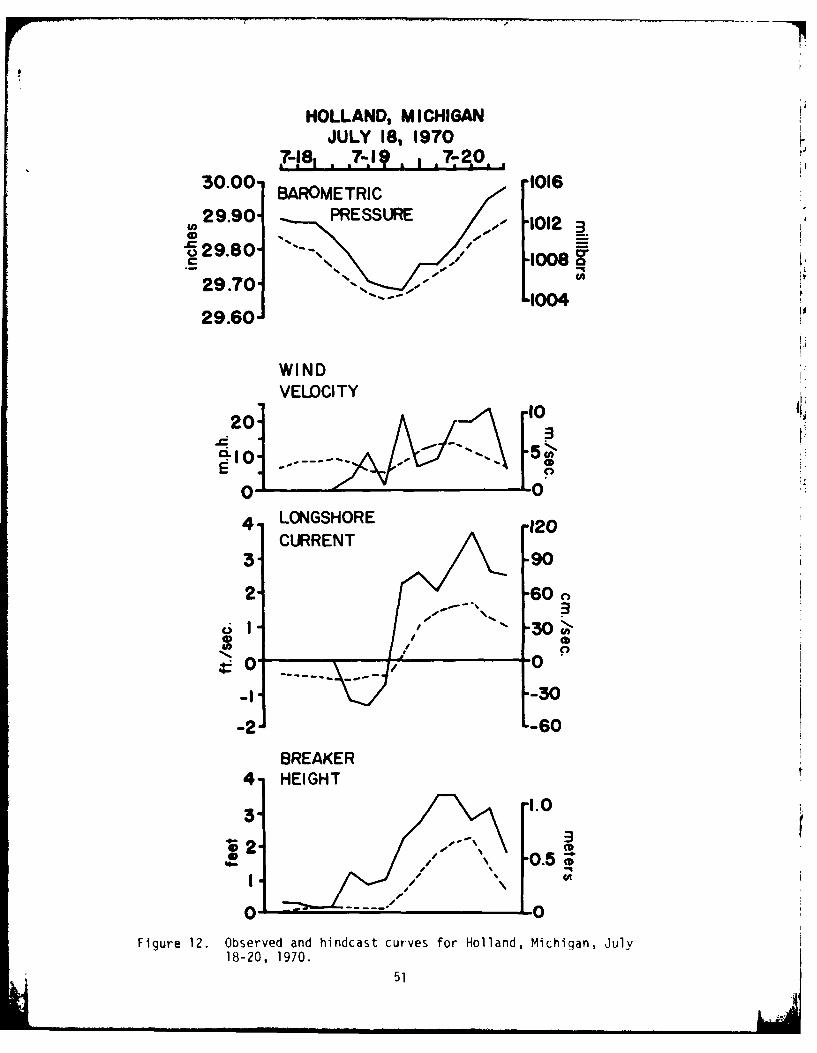
HOLLAND, MICHIGANJULY I81 1970

.7-18, 7-1I V *7-2*0. , *30.00- 1016

29.90-PESR

CM TRS RE'V 11

29.70-- 11004

29.60-

WINDVELOCITY

20-

4 LONGSHORE12CURRENT

3 .90

2 -601l .30

---- I 0oC

-1" -30

-2. -60

BREAKER4- HEIGHT

3 1.0

Z-

0-

Figure 12. Observed and hindcast curves for Holland, Michigan, July18-20, 1970.

51

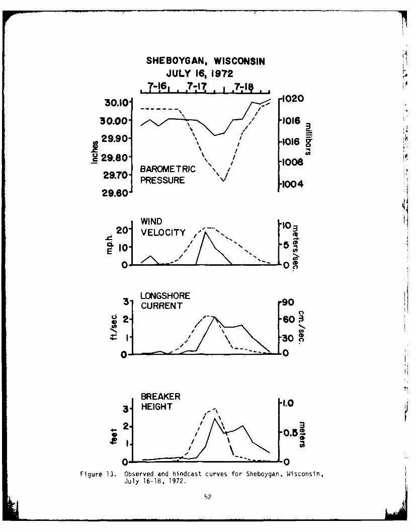
SHEBOYGAN, WISCONSIN KJULY 16, 1972

7-1, 7.17 . .7- ,

30.10 1020

30.00- "1016

29.90- % 1 /016

29.80" -1008

29.70 BAROMETRIC ' /

PRESSURE \ "00429.60

WIND *o020 VELOCITY

10-0. /-*x-"" -''"-o

LONGSHORE [

3- CURRENT 90

U 3 / 0

0 -0

BREAKER 1.0

3 HEIGHT I.0

* "0.b5

0 0Figure 13. Observed and hindcast curves for Sheboygan, Wisconsin,

July 16-18, 1972.

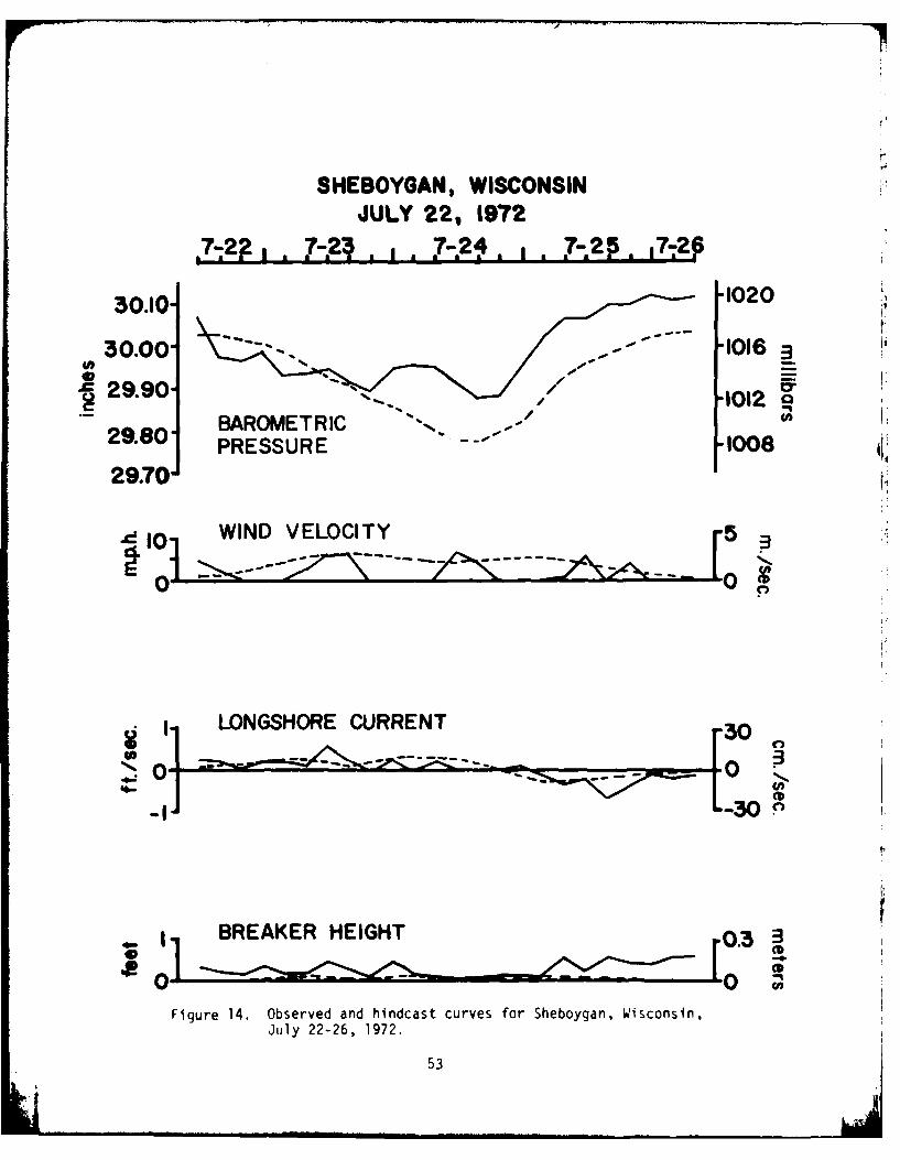
SHEBOYGAN, WISCONSINJULY 22, 1972

.7-2? 7-2 7-2 2 7-2 72

30.10 1020

3 0 0 0 " " " -,,, . ." "10 16

=29.90" C"--.. / "0 12BAROMETRIC - -2

29.80" PRESSURE -1008

29.70

, -/ - X--- - - - 5-- -

~ 01WIND VELOCITY5

Figure 14. Observed and hindcast curves for Sheboygan, Wisconsin,

July 22-26, 1972.

53

BREKE HEIGHT..0..

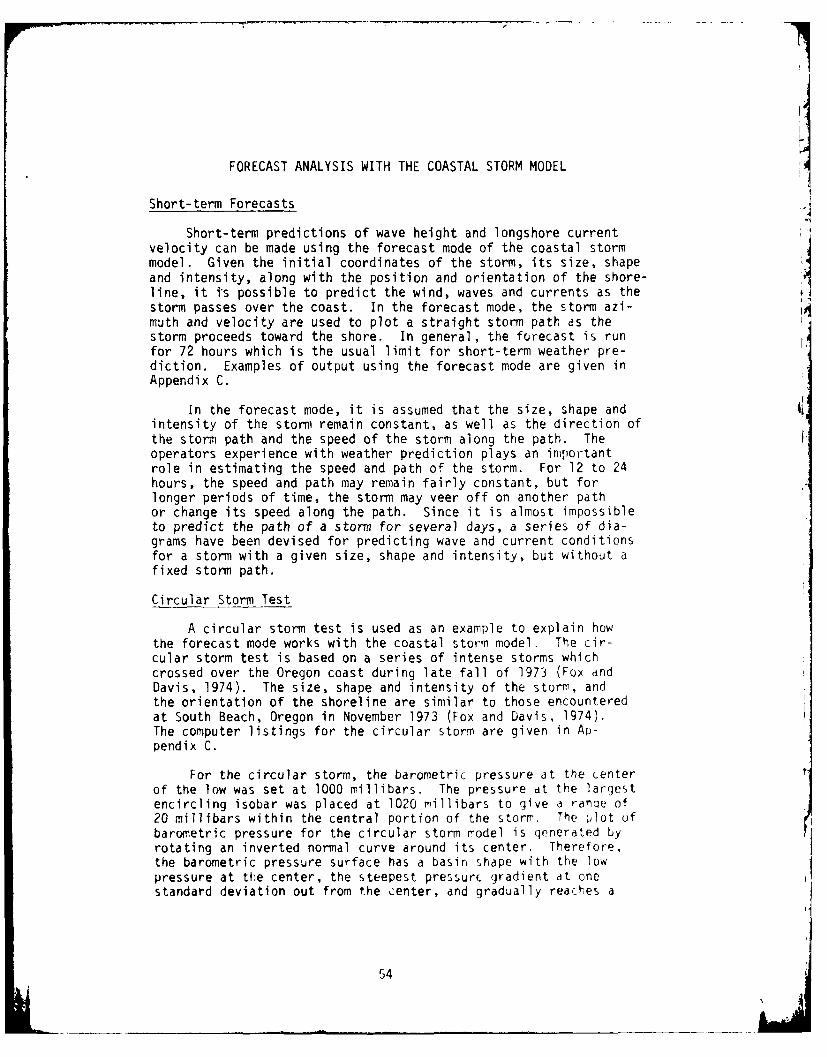
FORECAST ANALYSIS WITH THE COASTAL STORM MODEL

Short-term Forecasts4

Short-term predictions of wave height and longshore currentvelocity can be made using the forecast mode of the coastal stormmodel. Given the initial coordinates of the storm, its size, shape iand intensity, along with the position and orientation of the shore-line, it i's possible to predict the wind, waves and currents as thestorm passes over the coast. In the forecast mode, the storm azi-muth and velocity are used to plot a straight storm path as thestorm proceeds toward the shore. In general, the forecast is runfor 72 hours which is the usual limit for short-term weather pre-diction. Examples of output using the forecast mode are given inAppendix C.

In the forecast mode, it is assumed that the size, shape andintensity of the storm remain constant, as well as the direction ofthe storm path and the speed of the storm along the path. Theoperators experience with weather prediction plays an importantrole in estimating the speed and path of the storm. For 12 to 24hours, the speed and path may remain fairly constant, but forlonger periods of time, the storm may veer off on another pathor change its speed along the path. Since it is almost impossibleto predict the path of a storm for several days, a series of dia-grams have been devised for predicting wave and current conditionsfor a storm with a given size, shape and intensity, but without afixed storm path.

Circular Storm Test

A circular storm test is used as an example to explain howthe forecast mode works with the coastal storm model. The cir-cular storm test is based on a series of intense storms whichcrossed over the Oregon coast during late fall of 1973 (Fox andDavis, 1974). The size, shape and intensity of the storm, andthe orientation of the shoreline are similar to those encounteredat South Beach, Oregon in November 1973 (Fox and Davis, 1974).The computer listings for the circular storm are given in Ap-pendix C.

For the circular storm, the barometric pressure at the centerof the low was set at 1000 millibars. The pressure at the largestencircling isobar was placed at 1020 millibars to give a ranqe of20 millibars within the central portion of the storm. The plot ofbarometric pressure for the circular storm model is generated byrotating an inverted normal curve around its center. Therefore,the barometric pressure surface has a basin shape with the lowpressure at the center, the steepest pressurc gradient at onestandard deviation out from the center, and gradually reaches a

54

maximum pressure at 3 standard deviations away from the center.ISince the outer margin of a storm often interfers with other highor low pressure systems, it is assumed that the largest encirclingisobar occurs at 2 standard deviations away from the center, or2/3 of the total storm radius. Therefore, the total storm radiuswould be 1.5 times the radius measured at the largest encirclingisobar, and the maximum pressure at the margin of the storm wouldbe 1.145 times the pressure range from the center to the largestisobar. In the circular storm test, the pressure at the 2 stan-dard devidtions is 1020 and the maximum pressure included in thestorm is 1022.9 millibars at 3 standard deviations.

The size of the storm is determined by measuring the lengthsof the major and minor half axes of the storm For an ellipticalor wave-shaped storm, the length of the major half axis is mea-sured from the center of the low to the largest isobar, where itis farthest from the storm center. The length of the minor halfaxis is measured at right angles to the major half axis from thestorm center to the largest isobar. A circular storm exists whenthe major and minor half axes are equal. For the circular stormtest, lengths of the major and minor half axes are 300 kilometers.When the major and minor half axes have different lengths, theorientation of the major half axis is plotted in degrees fromnorth. Therefore, for the circular storm test, the orientation ofthe major half axis is 0 degrees.

For the circular storm model, the storm velocity is set at 40kilometers/hour with a storm azimuth of 90 degrees. This means thatthe storm will proceed from its initial position along a path 90degrees east of north at 40 kilometers/hour. Therefore, if thestorm is tracked for 30 hours, it will move a distance of 1200 kilo-meters.

For the shore position coordinates in the circular storm test,X is set at 1000 and Y is set at 0 kilometers. In the X-Y coor-dinate system used for plotting storm position and shore locationon a weather map, the shore site is located 1000 kilometers eastalong the X axis and 0 kilometers north along the Y axis. Theshore latitude for the test case is 43 degrees north, the approxi-mate latitude of the Oregon coast. The onshore azimuth is 90degrees which indicates that the coastline ru~ns north-south withland to the east and sea to the west, the same orientation as theOregon coast. The nearshore slope is at 0.033 which is close tothe average nearshore slope in the different areas studied. Avalue of 1000 kilometers was used for the average fetch which wouldindicate open ocean. If the average fetch is greater than thestorm radius , the fetch distance will not have an effect on thewave and current calculations. However, if the fetch distance issmadller than the storm radius, the waves will be fetch limited whenthe average fetch is less than the effective fetch.

In compiling the output for the circular storm test, the stormoutlined above was tracked along 12 paths normal to the shorelineand parallel to each other (Figure 15). The location of the shoresite, orientation of the shoreline, and three storm tracks aregiven in Figure 15A. The diagram extends 1200 kilometers in anorth-south direction, 600 kilometers to the north (positive) and600 kilometers to the south (negative) of the study site whichis located in the center of the diagram. The diagram also extends1200 kilometers in an east-west direction, 600 kilometers offshore(negative) and 600 kilometers onshore (positive) of the shore site.A time scale is included along the bottom of the diagram to indicatethe length of time in hours from the initial tracking of the stormto any position along the storm path. The speed of the storm wasset at 40 kilometers/hour, therefore, if the storm started at theleft edge of the diagram, its center would pass over the shorelineafter 15 hours and would move off the right side of the diagramafter 30 hours.

56

A.STORM TRACK ANO LOCATION MAP B.BAROMETRIC PRESSURE -MILL IBARS

I ~ 1022.8.0 SEA I LND 0'

100

A-STORM TRACK 200 :km. NORTH;

B-STORM TRACK 0_____. T%

WO - X00 SHORE SITEI

C-STORM TRACK 300 SOU

00

.)

-400 0 400IKILOMIETERSTER

010 HOURS 20 30 0 10 HOURS 20 3

Figure 15. Map of storm tracks and time-distance plot of barometricpressure for a circular stormI.

1)71

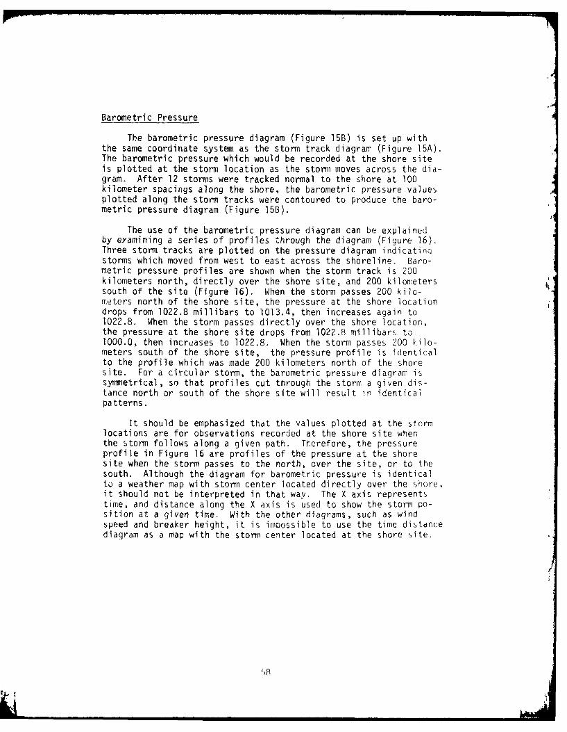
Barometric Pressure

The barometric pressure diagram (Figure 15B) is set up withthe same coordinate system as the storm track diagram (Figure 15A).The barometric pressure which would be recorded at the shore siteis plotted at the storm location as the storm moves across the dia-gram. After 12 storms were tracked normal to the shore at 100kilometer spacings along the shore, the barometric pressure valuesplotted along the storm tracks were contoured to produce the baro-metric pressure diagram (Figure 15B).

The use of the barometric pressure diagram can be explainedby examining a series of profiles through the diagram (Figure 16).Three storm tracks are plotted on the pressure diagram indicatioqstorms which moved from west to east across the shoreline. Baro-metric pressure profiles are shown when the storm track is 200kilometers north, directly over the shore site, and 200 kilometerssouth of the site (Figure 16). When the storm passes 200 kilo-meters north of the shore site, the pressure at the shore locationdrops from 1022.8 millibars to 1013.4, then increases again to1022.8. When the storm passes directly over the shore location,the pressure at the shore site drops from 1022.8 millibars tD1000.0, then increases to 1022.8. When the storm passes 200 kilo-meters south of the shore site, the pressure profile is identicalto the profile which was made 200 kilometers north of the shoresite. For a circular storm, the barometric pressure diagram, issymmnetrical, so that profiles cut through the storm a given dis-tance north or south of the shore site will result in identicalpatterns.

It should be emphasized that the values plotted at the stormlocations are for observations recorded at the shore site whenthe storm follows along a given path. Trorefore, the pressureprofile in Figure 16 are profiles of the pressure at the shoresite when the storm passes to the north, over the site, or to thesouth. Although the diagram for barometric pressure is identicalto a weather map with storm center located directly over the shore,it should not be interpreted in that way. The X axis representstime, and distance along the X axis is used to show the stormi po-sition at a given time. With the other diagrams, such as windspeed and breaker height, it is impossible to use the time distancediagram as a map with the storm center located at the shore site.

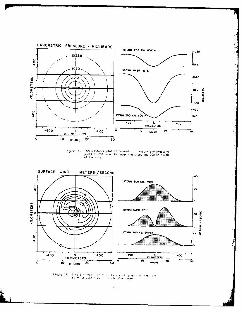
BAROMETRIC PRESSURE -MILLIBARS

I- STORM 200 KM. NORTH 1025

0 - ~- 1022.8 f/ 1110 1 20STORM OVER SITE

1 0 110000

n 1 020

0O STR 0 K.SU1010

-400 0400 HU1000

KKILOMETERS

0 0 HOURS 2'0 30

Figure 16. Time-distance plot of barometric pressure and pressureprofiles 200 km north, over the site, and 200 km southof the site.

SURFACE WIND -METERS /SECOND [40

STORM 200 KM. NORTH

0

00

KIOEER300 O3

1. HOR 200 OR

0lue1. h~-itveHto .l 'I~ed,~It'rfi2 fhn de ~a ''~-

0p

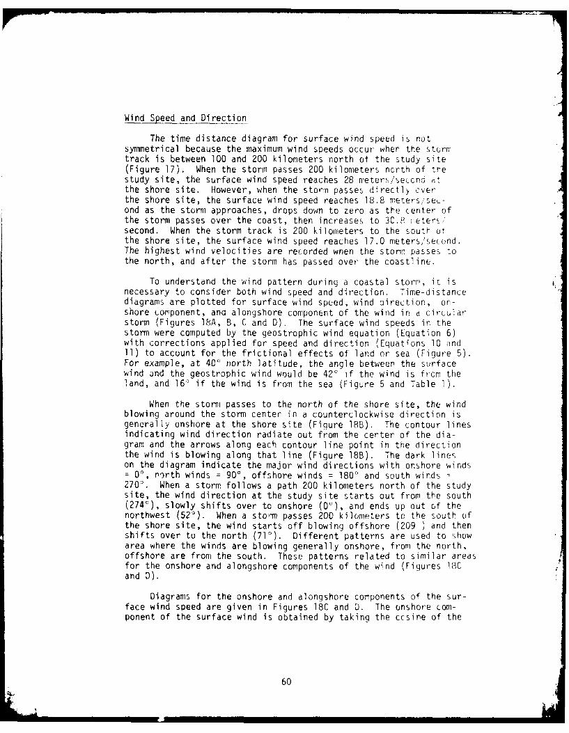
Wind Speed and Direction

The time distance diagram for surface wind speed is notsymmetrical because the maximum wind speeds occur when the stormtrack is between 100 and 200 kilometers north of the study site(Figure 17). When the storm passes 200 kilometers north of thestudy site, the surface wind speed reaches 28 meters/se(ono atthe shore site. However, when the storm passes directly cverthe shore site, the surface wind speed reaches 18.8 meters/seL-ond as the storm approaches, drops down to zero as the center ofthe storm passes over the coast, then increases to 30.8 -,eters/second. When the storm track is 200 kilometers to the south oithe shore site, the surface wind speed reaches 17.0 meters/second.The highest wind velocities are recorded when the storm passes *othe north, and after the storm has passed over the coastline.

To understand the wind pattern during a coastal storm, it isnecessary to consider both wind speed and direction. Time-distancediagrams are plotted for surface wind speed, wind direction, on-shore component, and alongshore component of the wind in d circularstorm (Figures 18A, B, C and D). The surface wind speeds in thestorm were computed by the geostrophic wind equation (Equation 6)with corrections applied for speed and direction (Equations 10 and11) to account for the frictional effects of land or sea (Figure 5).For example, at 40' north latitude, the angle between the surfacewind and the geostrophic wind would be 42' if the wind is from theland, and 16' if the wind is from the sea (Figure 5 and Table 1).

When the storm passes to the north of the shore site, the windblowing around the storm center in a counterclockwise direction isgenerally onshore at the shore site (Figure 18B). The contour linesindicating wind direction radiate out from the center of the dia-gram and the arrows along each contour line point in the directionthe wind is blowing along that line (Figure 18B). The dark lineson the diagram indicate the major wind directions with onshore winds= 0', north winds = 90', offshore winds = 180' and south winds =270'. When a storm follows a path 200 kilometers north of the studysite, the wind direction at the study site starts out from the south(2740), slowly shifts over to onshore (0°), and ends up out of thenorthwest (52°). When a sto,-m passes 200 kilometers to the south ofthe shore site, the wind starts off blowing offshore (209 ) and thenshifts over to the north (710). Different patterns are used to showarea where the winds are blowing generally onshore, from the north,offshore are from the south. These patterns related to similar areasfor the onshore and alongshore components of the wind (Figures 13Cand D).

Diagrams for the onshore and alongshore components of the sur-face wind speed are given in Figures 18C and D. The onshore com-ponent of the surface wind is obtained by taking the ccsine of the

60

wind direction times the wind speed, and the alongshore componentIis produced by taking the sine of the wind direction times thewind speed. Storms which follow a path to the north of the shoresite generally have a strong onshore wind component, while thosefollowing a path to the south of the shore site are predominatelyoffshore (Figure 18C). The dividing line between the onshore andoffshore components of the wind follows north-south wind directionlines (0' to l80')(Figure 18B). The onshore wind reaches a max-imum of 28.2 meters/second along a storm path 100 kilometers northof the shore ite. The offshore wind reaches 18.6 meters/secondwhet) the storm passes 100 kilometers south of the shore site andbefore its center moves across the coast. The onshore wind speedis greater than the offshore wind speed because the friction isless when the wind is blowing over the water.

The time distance diagram for alongshore wind component in-dicates that the winds are from the South as the storr approachesthe coast and shift over to the north after the storm passes (Fig-uire 18CD). To the north of the shore site, the shift in the alonQ-shore component from south to north takes Place after the stormhas pdssed over the coast, but to the south, the shift takes placebefore the sturm reaches the cuast. The boundary line between thenorth and south components of the longshore wind (Figure 18D) fol-lows the onshore-offshore line (90'-270') in the wind directiondiagram (Figure 18B). The reversal from south to north wind isvery abrupt near the center of the storm, and more gradual nearits margin. When the storm passes to the north, the low in baro-metric pressure reaches a minimum when the storm passes over thecoast (Figure 17), but the shift in wind direction f;-om south tonorth does not take place until several hours after the low haspassed. This lag in wind direction reversal behind the low inpressure was observed during storms at Holland and Stevensville,vhich passed to the north of the study areas (Fox and Davis, 1970and 1971a). Also, the maximum wind speeds were observed afterthe lows had passed and the wind shifted over to the north.

61

Figure 18. Time-distance plots of A - surface wind speed, B - winddirection, C - onshore wind, and D - alongshore wind ina circular storm.

62

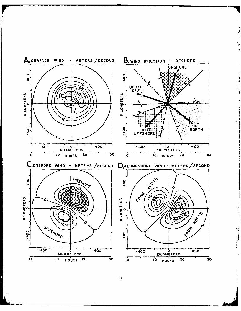
A-SURFACE WIND -METERS /SECOND B.WIND DIRECTION -DEGREES

~ NSHORE00

0 00

-- i

0' I-400 0460-io 6

i OS2030010 HOURS 20 30

CONSHORE WIND - METERS /SECOND D.ALONGSHORE WIND -METERS/SECOND

00400 0l

00

10,

ok4 -4

0

0.0 0.UR 20 0 3

_____ KILOMETERS___________ KILOMETERS

lbH'R 030 010) HOURS203

Wave Period and Breaker Height

The diagrams for wave period and breaker height are quitesimilar (Figures 21A and B), and both resemble the plots forsurface wind and onshore wind (Figures l8A and C). Three pro-files wiere plotted across the breaker height diagram to showwhat the height would be at the shore site as the storm movesacross (Figure 19). If the storm moves 200 kilometers northof the shore site, the breaker height will reach 5.30 meters3 hours after the storm crosses the coast. If the storm passesdirectly over the shore site, the breaker height will reach.86 meters as the storm approaches, drop down as the center ofthe storm passes, then reaches 3.63 meters 5 hours after thecenter passes over the coast. The decrease in wave height asthe storm center passes directly over the shore site correspondsto the zero wind velocity at the center of the storm. Whilewind velocity may drop to zero at the storm center, the zerowave height is probably an artifact of the computer model anddoes not occur in nature. Residual waves would most likely re-main in the area and could be built model if so desired.

The surface wind speed is not used directly for determiningbreaker height and wave period, because strong onshore wind iseffective in generating waves which will reach the coast, and astrong offshore wind tends to subdue existing waves. On the Texascoast during studies made at Mustang Island, offshore wind wasaccompanied by a sharp drop in breaker height (Davis and Fox, 1972c).On Lake Michigan, where a single storm system was studied as itmoved offshore at Zion, Illinois and onshore at South Haven, Mich-igan, breaker height was over 2 times as great where wind wasblowing onshore than where it was blowing offshore (Davis and Fox,1974b). Therefore, the effective wind speed was used in deter-mining wave height and period in place of the surface wind. Foran onshore wind, the effective wind is equal to the onshore wind.However, for an offshore wind, the effective wind is about onethird of the surface wind speed. For a wind blowing along theshore, the effective wind speed is two thirds of the surface windspeed. A cosine transformation was used to produce a smooth gra-dient in effective wind from onshore through alongshore to off-shore.

The plot for wave period closely resembles the plot for breakerheight with the maxima to the north of the shore site and displacedlandward of the shoreline (Figure 21A). The maximum wave period of9.5 seconds occurs at the same time as the maximum breaker heiqht,3 hours after the storm has passed over the coast. The plot forwave period has a broad relatively flat area surrounding the maxi-mum, while the plot for breaker height is much steeper, reaching apeak and rapidly dropping off after the peak has been passed. Thewave height and periods forecast in the model correspond closely tothose encountered on the Oregon coast during November 1973 (Fox andDavis, 1974).

64

Breaker Angle and Longshore Current Velocity

The plots of breaker angle and longshore current velocity(Figures 21C and D) are similar in many respects to the plot foralongshore wind (Figure 18D). The boundary line which separatesthe north and south components of the wind is the same as theboundary which separates the north and south breaker angles andlongshore currents. For field studies conducted at Holland andStevensville, Michigan, there was also a close correspondencebetween the longshore component of the wind and longshore currentvelocity (Fox and Davis, 1970a and b, and 1971a).

The breaker angle is defined as the acute angle between thewave crest and the shoreline as the wave passes over the nearshorebar. In deep water the wave direction is roughly parallel to thewind direction, and the wave crests are about normal to the wind.The dominate wind direction is often used in wave refraction com-puter programs to determine the deep water wave angle (Dobson,1967). As a wave enters shallow water, the celerity decreases andthe wave crest is refracted so that it becomes closer to parallelto the beach. Snell's Law of geometrical optics is used for com-puting the refraction coefficient and breaker angle in the surfzone.

In the breaker angle diagram, the area to the left of the zeroline has breaker angles open to tle north, and to the right of thezero line, the breaker angles are open to the south (Figure 21C).The largest breaker angles are about 32 degrees when the wind isblowing directly out of the north or the south. As the wind di-rection swings around from alongshore to onshore or offshore, thebreaker angles decreases from 30 degrees to zero (Figures 18B and21C). When the wind is blowing directly onshore or offshore, thebreakers are parallel to the beach and breaker angle is zero.

The plot for longshore current velocity is very similar tothe plot for the alongshore component of the wind (Figure 13D and21D). Three profiles are plotted when the storm passes 200 kilo-meters north, over the shore site and 200 kilometers south (Fiq-ure 20). When the storm path is 200 kilometers north, the Iong-shore current velocity reaches 97.4 centimeters/second to the north,reverses direction after the low has passed, and increases to 81.6centimeters/second to the south. When the storm passes directlyover the study site, the current reverses from 63.0 centimeters/second to the north to 129.7 centimeters/second to the south. How-ever, when the storm path is 200 kilometers south of the shcre JAte,the current to the north is only 4.8 centimeters/secund anu trcesouthward current is 58.1 centimeters/second. When the stc'r! passesto the south, the reversal in current direction takes place beforethe low in barometric pressure passes the shore. The maximum long-

65

let.

i

Figure 19. Time-distance plot of breaker height and three profilesof breaker height in a circular storm.

Figure 20. Time-distance plot of longshore current and three profilesof longshore current in a circular storm.

66

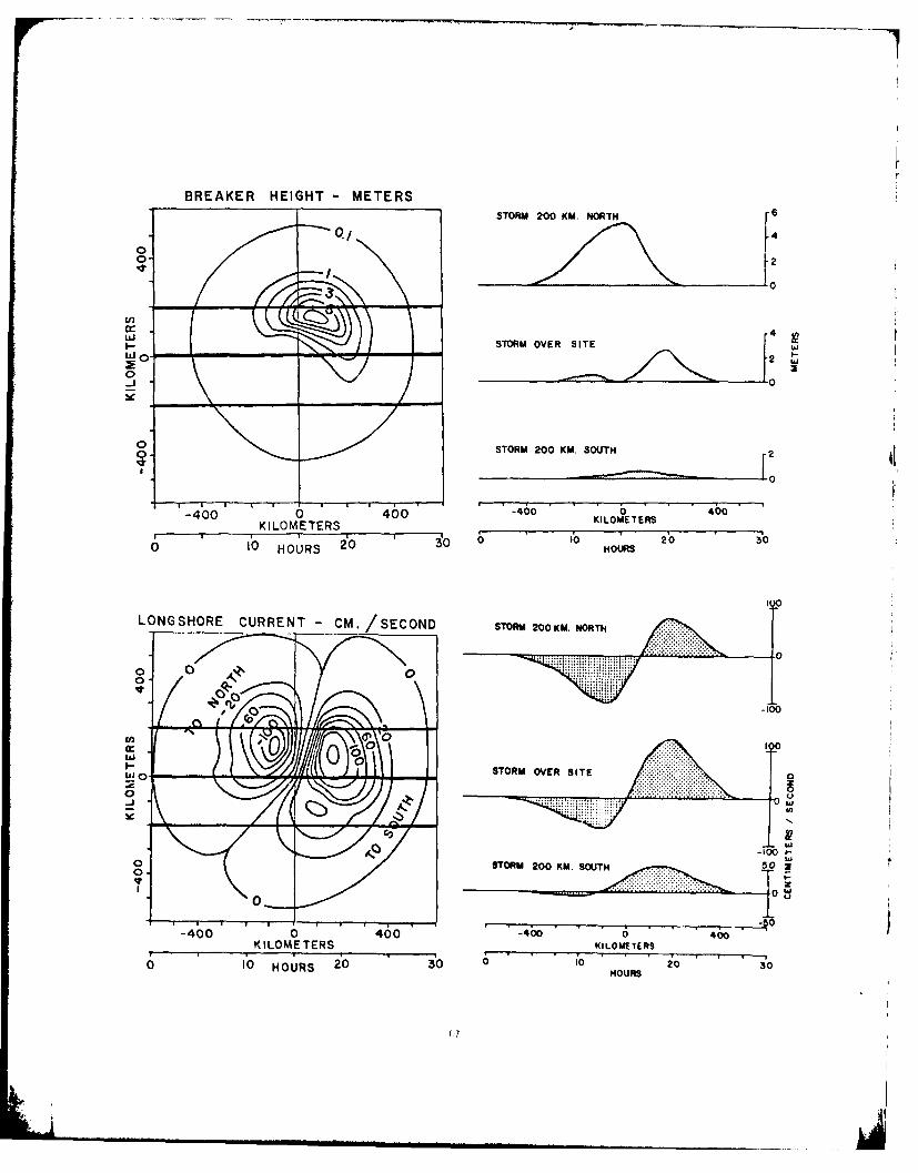
BREAKER HEIGHT -METERS

STORM 200 KMW NORTH6

cr -LUSTORM OVER SITE w

I- 1

0- STORM 200 KM. SOUTH2

-400 0 4b0-400 040KILOMETERS

KILOMETERS So ________b ______2__0 _____

lb HOURS iOHOURS

LONG SHORE CURRENT -CM. /SECOND STORM 200KM. NORTH

0)0

100

o~l STORM 200EK SUTH

00

040 400 -46 646

KILOMETERS KILOMETERS

0 0HOR 2 0 0 10 20 s00 10 OURS o ioHOURS

(7

Figure 21. Time-distance plot of A - wave period, B - breaker height,C - breaker angle, and D - longshore current in a circularstorm.

68

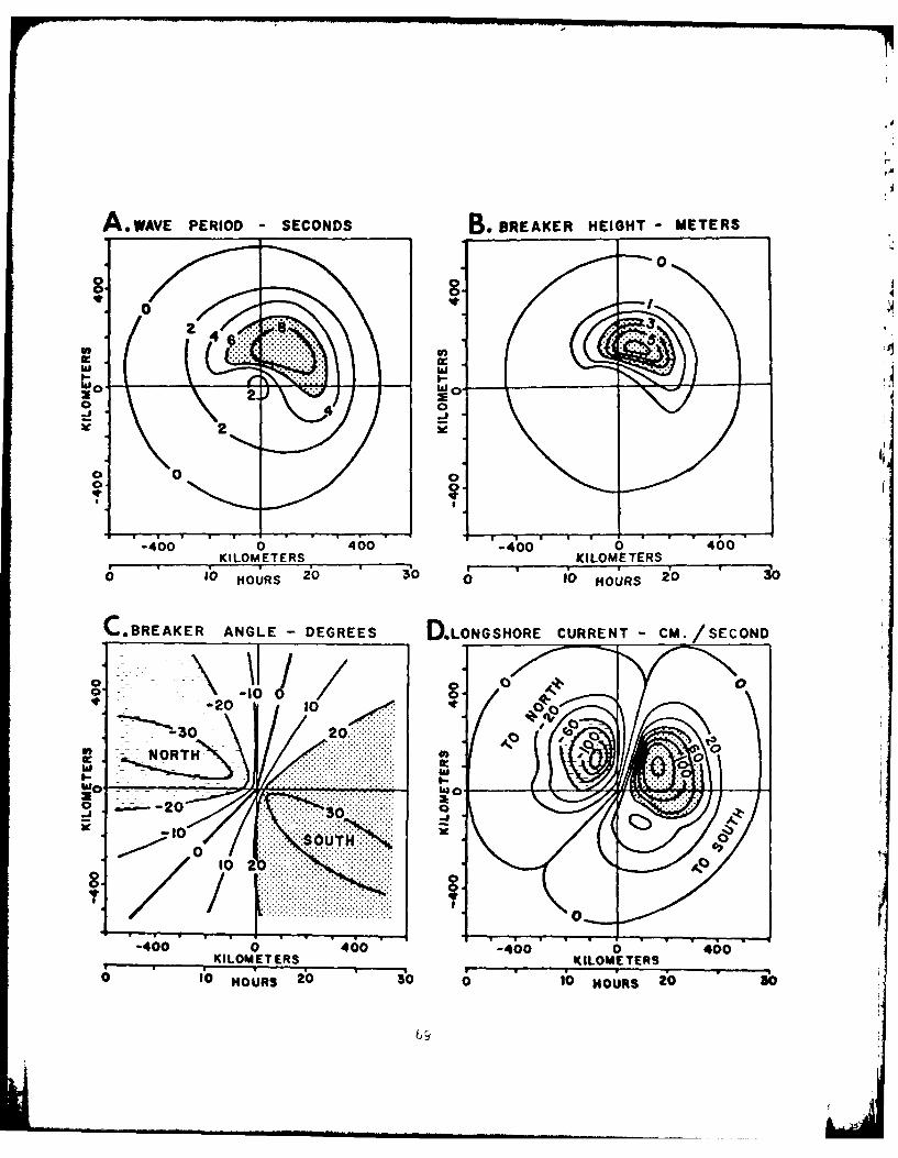
A.WAVE PERIOD- SECONDS B. BREAKER HEIGH4T- METERS

44

00

KILOMETERS KILOMETERSlb HOURS '0 -r 30 10 HOURS 20

C.BREAKER -ANGLE -DEGREES D.LONGSHORE CURRENT -CM. /SECOND

00N~ -100-20 10

-30 2

hi 0 -0

0 -- 20 . 0 . ...

-010

80

6 -00 KILOMETERAS KILOMETERS

otO HOURS 20 30 0 t0 HOURS 20 50

69

shore current was 144 centimeters/second to the south 4 hours afterthe storm passed over the shoreline on a path 100 kilometers northof the shore site (Figure 20).

The longshore current velocity is a function of nearshore slope,breaker height and breaker angle (Longuet-Higgins, 1970). The in-fluence of both breaker angle and breaker height can be seen in theplot for longshore current velocity (Figures 19B, C and 0). Otherlongshore current equations were tested which gave similar patterns,but different absolute velocities.

The circular storm test illustrates the general patterns whichemerge in barometric pressure, wind, waves and longshore currentsas a storm passes over a coast. If the shape and path of the storm,and the orientation of the shoreline are held constant while thesize or intensity of the storm are varied, the same patterns willpersist, but the absolute values will change for each of the vari-ables. However, if the shape or path of the storm are changed,the patterns as well as the absolute values will change for eachof the variables. In the next section an elliptical storm is usedto demonstrate the effect which a change in storm shape would haveon the wind, waves and currents.

70

Elliptical Storm Test

With the coastal storm model, it is possible to vary thesize and shape of the storm while holding the intensity constant.The elliptical storm test provides a good example of an oval shapedstorm which has its long axis extending to the north-northeast(Figure 22). In both the circular and elliptical tests, the shore-line orientation and nearshore bottom slope are the same.

In the circular and the elliptical storms, the minimum baro-metric pressure at the center is 1000 millibars, and the pressureat the largest encircling isobar is 1020 millibars (Figures 16 and22). In the circular storm, the major and minor axes are the same,300 kilometers. In the elliptical storm, however, the major axis(500 kilometers) is twice the length of the minor axis (250 kilo-meters). The major axis in the elliptical storm is oriented 30'east of north. Therefore, a low pressure trough extends in anorth-northeast direction with the lowest value at the stormcenter.

The time-distance plot of barometric pressure is identicalto a weather map made when the storm center is over the shoresite (Figure 22). When the storm track is located to the southof the shore site, the low pressure trough reaches the shore sitebefore the low pressure center passes over the coast. However,when the storm track is to the north of the shore site, the lowpressure center reaches the coast before the trough passes overthe shore site. Therefore, the long axis of the storm marks thetime when the low pressure trough passes over the shoreline.

Although the range in barometric pressure is the same in thecircular storm and the elliptical storm, the pressure gradient issteeper in the constricted part of the elliptical storm. The pres-sure gradient is a function of the size of the storm and the rangein barometric pressure. In the circular storm, both the major andminor axis have lengths of 300 kilometers, and therefore the pres-sure gradient is equal on all side of the storm. In the ellipticalstorm, the major axis is 500 kilometers and the minor axis is 250kilometers. Therefore, along the minor axis the pressure gradientis steeper, while it is more gentle along the major axis.

The time-distance plot of surface wind speed has an ellipticalshape with the high winds concentrated on the right side of thediagram (Figure 23A). The high wind speeds are a function of thesteeper pressure gradient along the minor axis and differences insurface friction over land and sea. With the higher pressure qTra-dient, the wind speed reaches 36.8 meters/second in the ellipticalstorm, while in the circular storm, it only reaches 30.9 meters/second. The winds greater than 20 meters/second are split into

71

two areas in the elliptical storm, a major area down the rightside of the storm, and a minor area in the northwest quadrant.At the center of the storm along the major axis, the surface windspeed drops down to zero.

The pattern for wind direction in the elliptical storm issignificantly different from the pattern in the circular storm(Figures 18B and 23B). In the circular storm, the wind directioncontours radiate out from the center and are rotated in a clock-wise direction from 140 to 450. The zero wind direction indicatesonshore wind and 180' is an offshore wind. The elliptical stormis constructed along the minor axis and extended along the majoraxis. Therefore, the wind direction contours are gathered aroundthe major axis which is pointed 30' east of north. Similarly,the contours are spread out from the minor axis. In the ellipticalstorm the zero contour extends 450 east of north, and the 180' con-tour extends 67' west of south . T he 2700 contour indicating southwinds points 17' east of north and the 900 contour for north windsextends 25' west of south.

The difference in wind direction pattern results in majorchanges in the onshore and alongshore wind patterns in the ellipticalstorm (Figures 23C and D). In the circular storm, the boundary linebetween onshore and offshore winds runs in a generally east-westdirection with onshore winds when the storm track is to the northand offshore winds when the storm track is to the south of the studysite. In the elliptical storm, on the other hand, the boundary be-tween onshore and offshore winds has shifted so that it runs general-ly north-south with onshore winds to the east and offshore winds tothe west (Figure 23C). As the storm approac.ries the coast the windsare offshore, and after the storm has passed over the shoreline thewinds shift to onshore. When the storm passes to the south of theshore site, the shift from offshore to onshore winds takes placeshortly after the low pressure trough passes over, but when thestorm track is to the north, the shift in wind direction shortlypreceeds the low pressure trough. The miaximumr offshore wind is21.4 meters/second as the storm approaches, and the maximum onshorewind is 30.2 meters/second after the storm has passed over the coast.

The boundary for the alongshore wind which separates the northwind from the south wind extends generally in a northwest-southeastdirection (Figure 23D). It resembles the alongshore wind diagramfor the circular storm, but the axes are rotated about 300 in aclockwise direction (Figures 18D3 and 23D3). The maximum south windof 21.1 meters/second occurs when the storm track is to the northof the shore site and after the storm has passed over the coast.For the north wind, the maximum of 28.1 meters/second occurs alonga storm track 200 kilometers south of the shore site after the stormhas passed the coast.

72

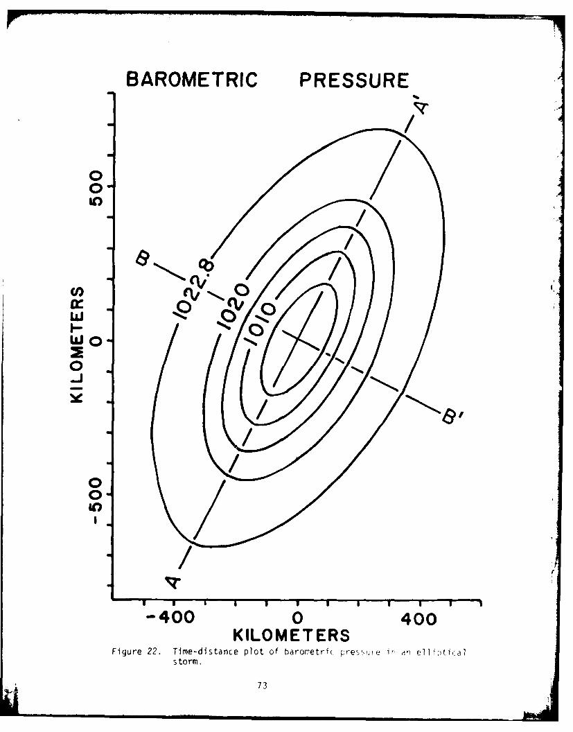
BAROMETRIC PRESSURE

00

SNO

Cl))wWo.

0

4-J

00

-400 0 400KILOMETERS

Figure 22. Time-distance plot of barometric pres iure iri an elliptic-alstorm.

73

Figure 23. Time-distance plot of A - surface wind speed, B - winddirection, C - onshore wind and D - alongshore wind inan elliptical storm.

74

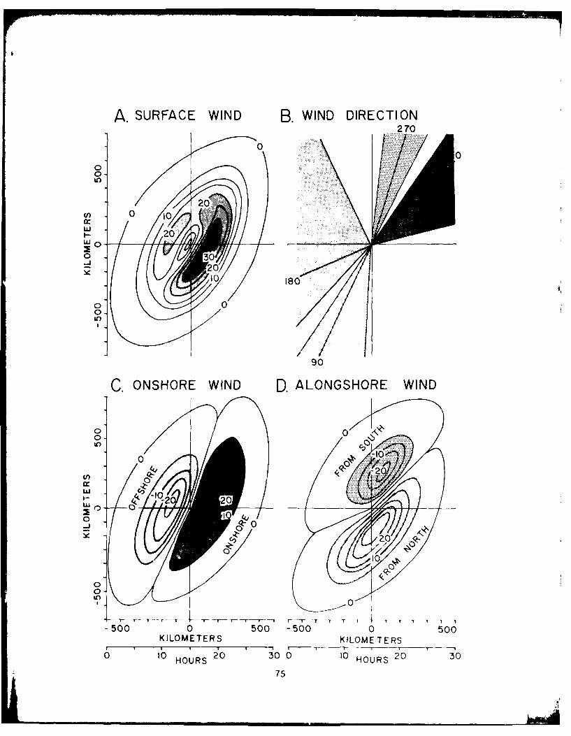
A. SURFACE WIND B.WIND DIRECTION

2.... 0.

200001

w

S0,

0

0.

C. ONSHORE WIND D.ALONGSHORE WIND

0

wF- 1

0-

~ T- I- -t r -T -- - ~ ri-- T r T I T 7 ---- 1

-500 0 500 -500 0 500KILOMETERS KILOME TERS

lbCHOR 20 30 10 H0UR5 2 0 30

75

IW

Figure 24. Time-distance plot of A - wave period, B - breaker height,C - breaker angle and D - longshore current in an ellip-tical storm.

76

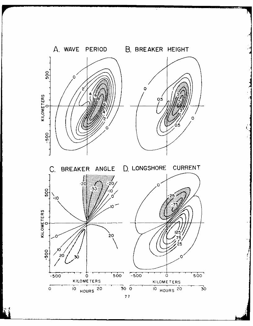
A. WAVE PERIOD B.BREAKER HEIGHT

01

0

-

00

0r0

wo

00

0-3

00

-10

KILMEERSKIOME0R

775

o"~ 10

2

The plots for wave period and wave height in the ellipticalstorm are very similar and closely resemble the plots for wind speedand onshore wind (Figures 23A and C, and 24A and B). Both waveperiod and breaker height reach their maxima after the storm troughhas passed over the coast and the wind has shifted from offshoreto onshore. In the elliptical storm, the maximum wave period is8.9 seconds and the greatest breaker height is 5.1 meters.

The greatest breaker angles for the elliptical storm occurwhen the wind is blowing out of the south (2700) or the north (90')(Figures 22B and 23C). When the storm track is to the north ofthe shore site, the greatest northerly breaker angles (32.3 ) arepresent just before the low pressure trough passes over the coast.However, when the Storm track is to the south of the study site,the largest southerly breaker angles (32.4') occur just after thestorm trough has passed the shore.

The plot for longshore current in an elliptical storm is verycrnmilar to the plot for alongshore wind (Figures 23D and 24D). Theboundaries between north and south winds and north and south currentsfollow the same line and the maxima are in the same position. Themaximum northward flowing longshore current (44 centimeters/second)occurs when the storm is on a track 300 kilometers north of the shoresite, while the maximum southward flowing current (143 centimeters/second) occurs on a storm track 700 kilometers south of the shoresite.

in summarizing the comparison between a circular stormr and anelliptical storm of the same intensity, the differences in baro-metric pressure and wind direction influence the other environmentalparameters. In the circular storm, the highest surface winds arefound when the storm track is to the north of the shore site whilein the elliptical storm, the maximum winds occur in a north-northeasttrending zone to the right of the low pressure trough. The boundarybetween offshore and onshore winds lies generally east-west for thecircular storm and north-south for the elliptical storm. For along-shore winds, the boundary between north and south winds is rotatedabout 30' in a clockwise direction in the elliptical storm. In boththe circular and elliptical storm, the wind direction contours radi-ate out from the center and are rotated clockwise due to surfacefriction, but in the elliptical storm, the contours are gatheredaround the major axis. Wave period and breaker height in the circ-ular storm resemble wind speed and form pods to the north of theshore site, while in the elliptical storm, period and breaker heightform linear trends to the east of the shore site. For both storms,the longshore current follows the same pattern as the alongshore wind.

78

CONCLUSIONS

A mathematical model has been developed and programmed for acomputer to forecast barometric pressure, wind, waves and longshorecurrents during passage of a storm across a coastal site. The fol-lowing set of conclusions can be drawn from the coastal storm model.

1. The shape of a coastal storm can be approximated with an ellip-tical model by specifying the lengths of the major and minor halfaxes and the orientation of the major axis.

2. The barometric pressure profiles along the major and minor axesof the ellipse are represented by a series of inverted normal curves.

3. Geostrophic wind speed and direction at any point on the earth'ssufrace under a storm are computed from the latitude and barometricpressure gradient.

4. Geostrophic wind speed and direction are used to compute surfacewind speed and direction over land or sea.

5. Wave period, height and direction are calculated from the windspeed, fetch and duration as the storm passes over the coast.

6. Longshore current speed and direction are computed from waveheight, period and direction, and nearshore bottom slope.

7. Wave and current hindcast data can be used to test the model whenthe size, shape,intensity and track of the storm are known.

8. If the storm azimuth and velocity are assumed to be constant, fore-casts of wind, wave and longshore currents can be made for a coastalstorm.

79

ZI

REFERENCES CITED

Baur, F. and Phillips, H., 1938, Untersuchungen der Reibung beiLuftstromungen uber dem Meer. Ann. Hydrogr. u. mar. Meteor.,vol. 66, no. 6, pp. 279-296 (cited in Godske et al, 1957).

Birkemeier, W.A., and Dalrymple, R.A., 1976, Numerical models forthe prediction of wave set-up and nearshore circulation: Tech.Rept. no. 1, ONR Contract N00014-76-C-0342, University of Del-aware, 127 p.

Bretschneider, C.L., 1952, Revised wave forcasting relationships,Proc. of 2nd Conf. on Coastal Engineering, A.S.C.E., Councilon Wave Research.

Bretschneider, C.L., 1958, Revisions in wave forecasting, deep and 4Ishallow water, Proc. of 6th Conf. on Coastal Engineering, A.S.C.E.Council on Wave Research.

C.E.R.C., 1973, U. S. Army Coastal Engineering Research Center, ShoreProtection Manual, TR 4, vol. 1, pp. 1-496.

Cole, F.W., 1970, Introduction to Meterology, John Wiley and Sons,New York, 388 p.

Collins, J.I., 1971, Longshore currents and wave statistics in thesurf zone: Tech. Rept. No. TC-149-2, ONR Contract N00014-64-C-0107, Tetra Tech, 46 p.

Davis, R.A., Jr., and Fox, W.T., 1971, Beach and nearshore dynamicsin eastern Lake Michigan: Tech. Rept. No. 4, ONR ContractN00014-69-C-0151, Williams College, 145 p.

Davis, R.A. Jr., and Fox W.T., 1972a, Four-dimensional model forbeach and inner nearshore sedimentation: Jour. of Geology,vol. 80, pp. 484-493.

Davis, R.A. Jr., and Fox, W.T., 1972b, Coastal processes and near-shore sand bars: Jour. Sed. Petrology, vol. 42, pp. 401-412.

Davis, R.A. Jr., and Fox, W.T., 1972c, Coastal dynamics along Mus-tang Island, Texas: Tech. Rept. no. 9, ONR Contract N00014-69-C-0151, Williams College, 69 p.

Davis, R.A. Jr., and Fox, W.T., 1974a, Coastal dynamics of CedarIsland, Virginia, Tech. Rept. no. 11, ONR Contract N00014-69-C-0151, 66 p.

80

Davis, R.A. Jr., and Fox, W.T., 1974, Simultaneous process-responsestudy on the east and west coasts of Lake Michigan: Tech. Rept.no. 13, Contract N00014-69-C-0151, 61 p.

Davis, R.A. Jr., and Fox, W.T., 1975, Process-response patterns inbeach and nearshore sedimentation: I, Mustang Island, Texas,Jour. Sed. Petrology, vol. 45, pp. 852-865.

Defant, A., 1961, Physical Oceanography, vol. 2, Pergamon Press,New York, 598 p.

Detrick, G., 1944, Die Gezeiten des Weltmeeres als geograph.Erscheinung Z d. ges. Erdkunde, p. 69. Berlin.

Dobson, R.S., 1967, Some applications of a digital computer tohydralic engineering problems: Tech. Rept. no. 8, ContractNONR 225 (85), Stanford Univ. 163 p.

Fox, W.T., and Davis, R.A. Jr., 1970a, Fourier analysis of weather

and wave data from Lake Michigan, Tech. Rept. no. 1, ONRContract N00014-69-C-0151, 47 p.

Fox, W.T., and Davis, R.A.Jr., 1970b, Profile of a storm-wind, wavesand erosion on the southeastern shore of Lake Michigan, Proc.13th Conf. on Great Lakes Research, p. 233-241.

Fox, W.T., and Davis, R.A. Jr., 1971a, Fourier analysis of weatherand wave data from Holland, Michigan, July 1970: Tech. Rept.no 3, Contract N00014-69-C-0151, 79 p.

Fqx, W.T., and Davis, R.A. Jr., 1971b, Computer simulation processesin eastern Lake Michigan: Tech. Rept. no. 5, ONR Contract N00014-69-C-0151, 114 p.

Fox, W.T., and Davis, R.A. Jr., 1972, Coastal processes and beachdynamics at Sheboygan, Wisconsin, July 1972: Tech Rept. no. 10,ONP Contract '100014-69-C-0151, 94 p.

Fox, W.T., and Davis, R.A. Jr., 1973, Simulation model for stormcycles and beach erosion on Lake Michigan: Geol. Soc. Nrer. Bull.,vol. 84, pp. 1769-1790.

Fox, W.T., and Davis, R.A. Jr., 1973, Beach processes on the OreionCoast: Tech. Rept. no. 12, ONR Contract N00014-69-C-0151, 81 p.

Galvin, C.J. Jr., jd Eagleson, P.S., 1965, Experimental study oflongshore currents on a plane beach, T M-10, U.S. Army CoastalEngineering Research Center, Washington, U.C., 80 p.

81

Godske, C.L, Bergeron, T., Bjerknes, J., and Bundgaard, R.C., 1957,Dynamic Meteorology and Weather Forecasting, Amer. MeteorologySociety, Boston, Mass., and Carnegie Inst. of Washington, 800 p.

Goldsmith, V., Morris, W.D., Byrne, R.J., and Whitlock, C.H., 1974,Wave climate model of mid-Atlantic and shoreline (Virginian Sea),NASA SP-358, V.I.M.S. SRAMSOE no. 38, 146 p.

Hesselberg, Th., and Sverdrup, H.U., 1915, Die Riebung in der Atmos-phare. Veroff. Geophys. Inst. Univ. Leipzig, ser. 2, vol. 1,pp. 241-301, (cited in Godske, et al, 1957).

Kauffman, C.F., 1973, Swell prediction by a multiple point-sourceswell generation model, M.S. Thesis, Naval Postgraduate School,Monterey, Calif., 73 p.

Komar, P.D., 1969, Longshore transport of sand on beaches, Ph. D.Thesis, San Diego, Univ. of California, 143 p.

Komar, P.D., 1973, Computer models of delta growth due to sedimentinput from rivers and longshore currents, Geol. Soc. Amer. Bull.vol. 84, pp. 2217-2226.

Komar, P.D., and Gaughan, M., 1973, Airy wave theory and breakerheight prediction, Proc. Thirteenth Conf. Coastal Engr.,1: 405-418.

Komar, P.D., and Inman, D.L., 1970, Longshore sand transport onbeaches, Jour. Geophys. Research, vol. 75, pp. 5915-5927.

Lewis, W.V., 1931, Effect of wave incidence on the configurationof a shingle beach, Geog. Jour., vol. 78, pp. 131-148.

Longuet-Higgins, M.S., 1970, Longshore currents generated by obli-quely incident sea waves: Jour. Geophys. Research, vol. 75,pp. 6778-6801.

Longuet-Higgins, M.S., and Stewart, 1964, Radiation stress in waterwaves: a physical discussion with application, Deep-Sea Research,vol. 11, pp. 529-562.

Louden, R.K., 1967, Programing the IBM 1130 and 1800, Prentice-Hall, Inc., Englewood Cliffs, N.J., 433 p.

McCammon, R.B., 1971, Environment pattern reconstruction fromsample data. L. Mississippi Delta Region, Tech. Rept. no. 1,ONR Contract N00014-69-A-0090, Univ. of Ill. at Chicago Circle,82 p.

82

McCallagh, M.J., and King, C.A.M., 1970, SPITSYM, a Fortran IVcomputer program for spit simulation, Kansas Geol. Surv.Computer Contr., 50, 20 p.

Munk, W.H., 1949, Solitary wave theory and its application to surfproblems, Annals of New York Academy of Sciences, vol. 51,pp. 376-424.

Noda, E.K., Sonu, C.J., Rupert, V.C., and Collins, J.I., 1974,Nearshore circulations undersea breeze conditions and wave-current interactions in the surf zone; Tech. Report TC-149-4,ONR Contract N00014-69-C-0107, Tetra Tech, Inc., Pasadena,Calif., 216 p.

Owens, E.H., and Frobel, D.H., 1975, Environmental, morphologicaland sediment size data from two barrier beaches in the Mag-dalen Islands, Quebec, G.S.C. Project 740009, Bedf6rd Insti-tute, Dartmouth, Nova Scotia, Canada, 447 p.

Putnam, J.A., Munk, W.H., and Traylor, M.A., 1949, The predictionof longshore currents, Trans, Amer. Geophys. Union, vol. 30,pp. 337-345.

Resio, D.T., and Hayden, B.P., 1973, An integrated model of storm-generated waves, Tech. Rept. no. 8, Contract N00014-69-A-0060,Univ. of Virginia, 288 p.

Snodgrass, F.E., and others, 1966, Propagation of ocean swell acrossthe Pacific. Philosophical Trans., Royal Soc. of London, vol.259, pp. 431-497,

Sonu, C.J., and van Beek, J.L., 1971, Systematic beach changes onthe Outer Banks, North Carolina, Jour. Geol., vol. 79, pp.416-425.

Sverdrup, H.U., and Munk, W.H., 1947, Wind, Sea and Swell; Theoryof Relations for forecasting, Publication No. 601, U.S. NavyHydrographic Office, Washington, D. C.

Westwater, F.L., 1943, Wind structure over the sea, Quart. Jour. R.Metero. Soc., vol. 69, pp. 207-213.

83

APPEND I A. WA ALC 5',M UPkpkMS

I'JOB//FOR

*IOCSICARD. 1132 PRINTER)

-ONIE WRD INTEGERS-LIST SOURCE PRZ-.GRDT.

COMMON U1130i.v1301DIMENSION TITLEIASI ,DAYITIDIMENSIONAIZ*A 2*A2iA421821.12*C11C12 CIIDATA Al/' 'A'. AU'/.A2,'DMET'.'TICA',.A3/'ERS '.'L MI'/.1 A4/' -*'LES '.1'MET'.' FEE' .B2 'CR5 *,T I ,2C1/' JOU'.' FOO'/.C2/'ES '.IT PO'',C3oI '.'oNDS-'

CC CARD 1 - TITLkCC CARD 2 - STARTING DATE, TIME AND INPUT-OUTPUT OPTIO NS

C COL$5. 1-2 ISTAT- STARTING HTOURC C065. 3-22 DAY - STARTING DATE

CCDL. 23 INAUT- INPUT OPTIONIC 0 METRIC iNITsC I NAUTICAL MILES AND FEETCC COL. 24 NAUT - UTPUT OPTIUNC 0 METRIC UNITSC I -NAUTICAL 'ILESl FtE' AND ONDTACC CARD 3 - STORM PARAMLTERSCC COL. I STORM INPUT OPTIONS - bLE CARDC I * INDCASTINQ, - TORM POSIT IN. AT A HOUR INTLC 2 * POECASTINS - INI'IAL POALTION. AZIMUTH ANDC V EL 1,0IT,

CCOL . 2 TIDE PREI.CTIoN OPT IONC 0 TIDE VELICT ION N-T INCLuDED - -,IT CARL 4C I *TIDE PREDICTfION INCLIOED - SEf CARD

C COL. 3 LJNSS'SORE CURRENT E,A'ION CPTIONC I * UX AND OAvIS. 19T2C 2 * NOLET'sIDjINS, 191CC 3 *L.E.A.C.. 191,C '. K -OMAR AND INMAN. 1970CC COLS. AAb NA - NuMBER OF STAM POSITIONSC IV H00R INTERVALS. F,. 'IGCSTNC ONE HOUR INTERVALS FUR FO)RECAITINMaCC COILS. 7-12 RNPCH- AVERIAGE RASIN FETCH IN &M. (NAUT. MI.,C CL.13-17 TI'-' - TIME INTERVAL bETAFIN STORM PLSI'II.NSC N/jAMAL SETTIN, Is, 1.) HOURS

(01$. Ir-AL LP'IN - MINIMUM PARLMETRIC PRESSURE IN MILLIBAMS,C .01. 5-jI I'HAAN PA

1SACU AT LARUEST ENCIRCLINQ ISobAR

C C 5, . 3JP-l tAT - L A TI .JOE AT I5 URE SI1TELC

c .. ST/sM SIZE *

CA-.. -5 S - sT'<N. "AF-ANIS, IN FETv k lbI

C AS. LALT - R L ' 'A ANGI L " 'ECT- X LIb0

-Ib 9A A RAT -I'" SPMI TUE

AR'- 4 - t UEIDINA TIDET-1 ~ wL14

-,'D kA E& INRFL~L'

L I''''R 'AS FV - LARST ~ILETO- AT .;,.HI. AT il'tIL

'-'AS-~; NA V,7I SILItFE

- - -. NA'sIN NAVA ll'A

NA 45; %A V.4,I ,F

N!I- Lk'~'- - HA-SAIE lSLANZ

- 'BN- "AI'.'4

6 M ',A ,A

S INAsWA. AIS

c C; .5. 1. l - 512AM A-l!, - CLJCIE F NW IyT",C, O.S. I5-41 1l - INITI'A'L ' X.C.DINATE IN N'AIICAL RIPS iC %K L.ULS. 2-M NI - NTIA( -OAJNT IN, NA,? IC LMIL4

** 925

(P." 26L * d

8031 HEAD :291,5, TITLI

915 PORMATIDOA..kITE 3. 91 : TITL.E

MiEA LI2,91 SI 1T!.1AyNAu,NAyT90' PORAATI 12.5A'..2!

IFP1NAAT 1.-2

2 '5! A L T 11.1 1.12

C CF.NI.C0

C ".MP * 'Ij L F IT T * u U . . T CU

91b ',RAT ZX.,N %'.N AT HCLII '.2. '.5A41MEACt2.901 )INQFT.IPTIU.LSCOP.NA'4NPCA,.T INTPMIN,PMHP5A7 AI.A.A.

NP CM NF C 1C A

iAl'-LLTkHI AANLaSAAN AT LAN(LLS ENCIkCLINu IS~bAk Is ASSLAHAL 1..UAv ,j ,TA'%D(&K- LLAIATNI. S P.'QM T. 17F' ~ T~..T.

C F IND Tl A T~A V, H"' 51-.', Tb t AAA.JH, ANLI MlU~AXI RET I.SI A T fl' LAI." '"SR Is M.I'1EOA

1 1'T '. S'yk A! I.E mARUIN TF $TV UTOM.

... 'A'TM..PC.HMI.T ME AI

P~~~~~Ul M'.7 I T.'- AM IC AAE!S..JH AT CENTS" CFALU. *.F .ILL 'MA'S 9''',tSC- AT tAAWGST LNCIAA...INU 508A R 0'1- AA' A" AIMM L'H1 I5Aj IN -.DE I N !,HA 'k

.LAI

IV. ' "CA CA'E. I EC.AT E.N FROM N AOD,l5.19

9I I' -Q T % H.F-'J DA J

A 7 '" ' SA,' "y "~P '0

AA[LN'. LA''I N FkyM . I .5,1913''~b. 73

' - ,A -,4. 4kt,'AIN .. 47~

A ., 1'A 1.b4N AH'g' FMAA ANLD I NMAN. H19 T,,I

AR A. %' A., .A..I S 41 51M VU , T.,y DTANUAAD (LtIATIIoNS .. .

IL' SCRA'Z I .CI2PF.

C.IA '' N"

AIL SASIR"AjTINES, FOR M1I4DCASTING AND0 IPVACASTI1N4, LIOtM

'A MNs'KA

-C

.0 DO. I1N

JLOCULO(.tA

v..OI>VLOX/A

L .V IA05

L . U DC ,AVL*VLOC.A

C

C wftIT

E 5MORE AND liDt DATAcAUL1*ULCCN.:05VL1 VL *Ck(N 05SNFC1.BNFCM.CKN17ITE97 lflLI.VL1,AUNNI.lA2(N.A3NN )A,NCSLATbAL.LOPE.

97L FCRtMATI 5S'1k( - PQS[T ION COORDITES F I, 7..I *T1I~~ RA C ArOE AILO -, "F .3' AO7 WS(JRL AZI..TI1

2 *:Ft.. D ELtCI'i,S'NEARbHORL SLQFL * ~.. ALAJ ~C F'

9 FQA' TI',C OFAIN TIJ AS. *~.: EL IL VN

'0 A I NA L c .IWr NUHI'.7'

A T I

'7'' .-I' 3.93:

AL T*''':.L*11.1 C~

t .. '.1 7..t .. '.',A ',',.'LA '. TE'Mb,'.K

B.14 T INLS.,'T.L ' I NE ,T' ... 'MAN '.TE, M I ND '5L..'

7 7'A 1EAZ- : ' A.1 ,

AN T TC AT -t ,AA, ,

TI

NA , tN'. .

U wAP.L.TT,.LAN

E 0

L A . -I - 411

N3A :, l '. 36

4"AN -IaN

Al 'A-S..' LS "76-

S. 7 7. A. .. ,5.7 .,.AE7 Nis,

EStJM.ESWM-E

UPT -U I It A C6N S

oSRF.ASLJRF*CKTS 'AL ALSM*CKTSEF.EF N ,.CKTSHI: .E IGT*CMF

T1D1.T [DX CMFV1*VLS*CCMF

11 TPCPU

1 IB1BRANG.V1

530 fORMATIX TL2*.;)2F?.G2F.2.4Fu.12,..F.po.FFhFlzfi, .*fIIF1ITIDT.QI WTE3

1 1 1401

sO: JMATI14,:.r.

Ie CDRIT:'E .11NT

C - sC T "w ENE

E !1CT:.ELSCT.SCUCUw,

E N" NE jOUL

R IYTEI354C) ESUM,QLI NN)I.CZI NN) *C3INN).ELSC T CI INN i CI NN I tA i NNI5.3 FOUM ATIIJ.// .ITsW AVE E NE Ry IN T4HE B REAKE R ZO0NE *E10. 3A8/,

1, TTTL LONC, _5HORE C URRENT ENERGY ,-E13. 3 .3A./IIW RIT EIt3.1 EP. V. *CNI *C3INN1,E,.oI " 155 *.CZN I *C3I 1.N G542 FO0RAT1..ZTL PO SI TIV .0G-SHORE CURRENT LNERt, ,ELG.3441/AT', TOTAL NEUATIVE LONUSHyORE CURRENT ENERGY 0EI.3,3A4)GO TO AS06C

'CO CALL EXITE ND

*SELETE 1: k,

JOB F18ORE 3-Ob-GO:IFOR

IOUCS1,.ARG.,132 PRINTER)

:ONE .08D :NT EGER SfLIST SOUVC E PRQGRA"

SUBROUTINE Ct(NA.A.NUTICOMMON I1,301.Vi1351

CC FGRECA5YINU - COJMPUTE STORM POSITIONS FROM INITlIAL POSITION.C VELOCITY AND AZIMUTH

TINT.1.0RAD5 1.29518

REFAD(2.90b) SVFL.AZI.VUII.V(903 FORMAT.LF 7.01

1 A8IEI3.G SVE..VAZI99X0 FOMA RA'TORM VEL IITY .F4P.0.' KILOMETERS/MUUR,

1 NA'STR AIUTH -',F4.o/IGO TO 0

R wITEi3.911 SRE.,AZI911 FORMA(AX, ST ORM IELOCIT, '.F4.0.' KWOS'

" IX.TRM Al - I. *-.F4.C/I5CONTIN UE

OIGT.-SVEO-T INT/RA IM.90 .-R II FIROZMI ,311.33

31 AZR .AZ7M. 3R5,32 00 35 1.NY.

UI' 1)-l *SIS SNAZM/RAGI

I5 CONTINUERETU U

8 N

END'2 UP

DEI.ETE FWE*STC&E * A 'Oki

"18 jO ING 3-86-0UIF, F5

-LIS' 5OPAC PROGA5j88., u T NE MIN1LOINIA I

7O~%Ut 1I301.1,1301

-33N1. %~j,1130)

4: CA 5T:3 - 7'U'L 5T1, R POSU5 1 NS A T HUwk I NTIE RVD0L 11 ?F6, 0U% P~IIN N EAHER AP

DO 15 '1.5AT' p

4EA>/N2 11

972j R ATI2FT.O

15 2- 111

D. vI -VII)tj/.

00 2O J. 1.

UImI.LJIM-1 .DIFUV(MVM. II.OIEV

IIM NUb-

vi YV NA

N11 iRETUR AN(NO

:DELETE W INDSATORE SA UA MIND

1i JOB0 LAT 3D6D01 A

11 FOR.lOC~l CARD, 1132, PR IN'TER)I-ONE WORD INTEU 1NA-LIAST SOURC E PkROGRAM

SUJBNOU JTIN E LOCATIlUATAVATAULOLA.LLICASHAIZ#XAYEAZAP,JI

CC U AND V COORDINATES APE LE AD INTO THE PAOGRAM IN KILOMETERS AM.C C ONVERTED TO0 UNI TS PRDPRTID0N AL TO ,H E WMAJOKA AXIS. THE U AND A

C CO0ORD INAT E SY STE M IS A RLICTANJ-JLAA C0 .JTI "U F0 POININ, LAST,.c v POINT I NG NORTH. A.'AU I. E UORILIN LOCATED TO THE SuuT;, EST OF V..E

c SHOV ,E LO0CAT :ON.

'" OuQTINE LOCAT.. Is USED TC EtSVTv..Iv '7E A ANDM ' Coo RDINAT Ec S'STEV W.1T V.E AIIS AT VHL LN IL" , VHL STRM AND~ UOS IVTIA.

'UI. F,' FAU' ~ E\~ N NE,A'IYE A Tc, THEPLEFT FA l'.,

RAG'. A-TA ANVY

AA.A _"'A RA.

A .SA,' CNA,

C ' -E 1 9 0.-v'AZ

AZLAR-DIF IWA

PDUP*DELETE LOLA?

'STORE AS 4A LOLA'

1P A E6 CSTA' 2-LOCALCSTRM.LOCAT,WIND.UELAV.EVIML.FETLH,.AES.UF .L*.AA'.TIDAt,INO.-L UC ALF "RECHOLLAND. YICHIGAN1IWULV 7. 1 97 0

101 21 150. 1.0 .1000 . 5. . .033

PP JOB [LI'S 1-86-L;&PP FOR.* ICSI CAMD 1 132 'A INTER I-ON' WOIRDRINTCEVS-LIST SOURCE P RILIAA

SQjB4,)uTI NE EL IPS ABAILIA"AIAEAADAA.A.,2A

C UBROUT INE (LIPS IS .SE I l 't 4 i"T VF IN ~ . U IASC. RAD IEN' XT ANY p-.I"T .1?'.' ANl L .IP'I(AC. ATLA'

.A0.%T.,95

A 'SpA

A- A

AAND1 AWLE THE VA. AN' MNOA4 ALE' 1, lTE SV..RM ELLIAEC , PINT Xl.I L I ES NASE. l LL!TI- ALE A, N~

'0''T~ A-IIA A 1.-i-Al

A '~ N~A( IN~iV4 AI AV LINE NORAA TC. 'HE

Vi-...I *.8 .Ln

C A AN. 2 Akt A' T.4 1NAS' 1N ,F ''E I NLAA, VT T"EkAC -'L,'' >' Vt DECAL, E~A, .C. A -L 'S.

2 , '7. ,

AiH,2 *D

FDA)A. ,T.A) .A-A

C ,Tt TEL TAN-N fIt TH5~E AT: , T CXITPANTD 11 % ~ MA C..AI,E

- , -I .eA ..

fAtN 11 T1. AL PA T lAN A DTH.S. T . , IN..

I ) II rOJAIY... 12 T12

LA.

-RXE *s a LPS

* !QCGCATJ,1;132EPRINTE.)

ADAt _vnDi IN ILGINSIS S ,JA PH STA"

GJTP .1 NA ,IN(AH,,'pHIN.PH AT,TAT,A,NF.A.SH*UNSH, GHAl-,LA.I AA.,YA.CHAZLAZ,DZA.ISN)E'NDI

7 IN -I -~ T1 DEP INE 7HA SL2 ,riIC .I NU SPLED

'N- :' : T , HANl IT 111 PKTE$j't bkAL)I E NT. T HE SLAFACL

Cl 1" C.1- 2 L E SVI-i,C nINO. THE ONSH.'II "Z",-N t )GGA CQP NT1 cC Ti . ND.

"A~I I ~ L.I 4C 1 ,-~ AT HEIGT, PLR.,

",l'L H, -'. 1 mcJET A..N., A NOIAA C.TAL IS, flLi; 1

L -L - 7~'I *..Gl

A * P' I: ) A - A

A L ' TA 'AN AA

- U * A N y A

AN T,2 ,ANA -&G

4V A A, TtTI:-N VA( V t GED - U DTLEkMINE GmA~I SI'.

G1 A'IH1LT F E T A PA:C. wI. i AN AND A

A. . . AN.A A

- A 'TI I C

AVIS e C PEA IAAAEA I THE SiP A-I L

2" . DO' ,5

N NS , - :

A - 75 AASI. ~ .5 E ' k DERE *A N .I

AO-AOB7 858 WILLIAMS COLL WILLIAMSTOWN MASS /RaCOASTAL STORM MODEL. (U) /42APR 76 W T FOX. R A DAVIS NOI-fi9-Co

UNCLASSIFIED TR-14 N01 C05

2,hEEhhEEE

C29 SINS-SINISAN6/RAO)

ZFISINS-.SI 35.30.3030 B;;00019

BEA;29.GO TO So

35 l:!91NS-;S) 36.40.403 6 B..0006

BETASOGO TO5 6;

40 ZFISANG-90.1 41.41.4241 SANA-SANG:3.,

GO TO 4842 1 F(SANG-10. 43,43.4443 SANA;I@O.-3.*1180.-SANG)

GO TO 484.4 !F,4SA7G;!70:!(4:4.!4.j45 SANA; So -3..SAG18I.

GO TO 4846 SANA 360:-3..1360.-SANG4(48 B=O0 $7..S5SIIAMA/RAO))

RETA*39.B-1O. B*SINISNARAD)

SJ SETR.BETA/RAOCOTA-SjNjBETR;lCOSjBET R ICOR/IB*CDSlBETR)ALPHAATN , ./COTA RAOIF(NX) , 1.5.52

51 SHAf4G.WANG*9.-A.PHASANG- SANG- AL PAN5.1GO TO 27

52 CONT4NUEVHCOR. COR*SINIALPHA/RADI/(B*CDSiBETRI)WSuRF .VHC OR*WSGEO

CC ONSHORE AND LONGSHORE COMPONENTS OF THE SURFACE WINDC

ONSH:"URF:COS ISHAN./RADIALSH WSURF SINI SHANG/RAD

CC EFWND IS ITHE EF ECTIVE WIN SPEED USED IN DE TERMININCG WAVESC AN "OFFS4MORE WIN IS ASSUMED TO BE .3 33 TI MES AS E FF CTIVE IC GENERATING AVS AS AN ONSHORE WINO.C

EFWND.W..JRF.( 6667+.3333.COSISHANG/RAD~ iIF(SHANGI 55,;0,60o

55 SHANG'SHANG+360.60 CONTINUE

IF(SHANG-36O.) 70.70,6965 SHANG-SHANG-360.70 CONTINUE

RETURNEND

II up*OELETE WIND*STORE WS UA WIND

IIJOB DECAY 3-86-001IIFOR

*IOCSICARD.2132 PRINTER)

:ONE WR INTEGERS*LISTWSOURCE PROGRAM

SUBROUTINE DECAY(TINT,PEROD.HEIGTICC SUBROUTINE DECAY IS USED 10 FIND THE DECAY IN WAVE HEIGHT ASC THE WAVES H OV E A WA Y FROM THE S TO RM CENTER.CCC ... FIND LOGARITHMIC ATTENUATION COEFFICIENTC

FREU.I./PERODATCOFZSO.*;!j!FREQ7O00611.O032,,1I-.)IF(ATCOF.G 01.D ATFlOIF4A TCOF.LT.O.1 ATCOFO.

CC ... FIND PROPAGATION DISTANCE IN DEGREESC

DIST-1.5607.PERQD*T INT*3SO./40074.CC ... FIND DECAYED WAVE HEIGHTC

HEIGT.HEIGT.I 2.71S3I*0I-2..IO.11Sl'ATCOFI*DIST I

R ETURNEND

*DELETE DECAY*STORE WS UA DECAY

i o8 ETIME 3-86-001IIFOR*IOCSICARD.1132 PRINTERI'ONE WORD INTEGERS*LIST SOURCE PROGRAM

SUsROUTINE ETIMEIWSNEW#DLDHHOURS.DRATNI

Cc SU9ROUTINt (TIME4 IS USED TO DETERMINE THE EFFECTIVE FETCH ANDC 3URATION FO TME NEW WIND SPEED FROM THE LAST PREVIOUS RIND SPEED.CC ... CONVERT M to FT AND M/SEC To FT/SEC

90

CH-OLDH/0. 1048WS-WSNEW/0.)OAB

CC... FIND EFFECTIVE FETCH USING MEW WIND SPEED AND OLD WAVE HEIGHTC

U.I (32.1OHI/IO.2830WS*.Il

DO 10 K.1.51.Z

SUM.SUM+U* I/ I10 CONTINUE

F.(WS**Z./32.1 ?'I5UH/O.012bIO'2.30CC... CONVERT FROM FT TO NM AND FT/SEC TO KTSC

F-F/6OTA.WSKTS.WS*3600. /AT76.

CC ... FIND EFFECTIVE DURATION USING DERIVED EFFECTIVE FETCHC

EFDUR-IF/I (WSKTS/1O.I**eO.TZ10.**0.3iI.*O.BDRAT N.HOU RS.EF DUNRETURNEND

IDUP-DELETE ETIME*STORE WS UA ETIME

/ JOB FETCH 3-86-001FOR

*IOCSiCARD.1132 PRINTER)-ONE WORD INTEGERS-LIST SOURCE PROGRAM

SUBROUTINE FETCH(A.B.XA.'vA.FlCC SUBROUTINE FETCH IS W4,S0 TO FIND THE EFFECTIVE FETCH AS A STORMC MOVES ONSHCRE OR OFFSHORE. THE FETCH LENGTH IS DETERMINED FROMC THE FETCH AREA WHERE THE WIND IS BLOWING TOWARD THE SHORE SITE.C THE EFFECTIVE FETCH$ AREA IS AN ELLIPSE WITHIN WHICH THE WIND ISC BLOWING AT GREATER THAN HALF THE MAXIMUM WINO SPEED. THE MAXIMUMC EFFECTIVE FETCH IS THE MAJOR AXIS OF THE ELLIPSE.C

FMAX.5$d8X1RP1.3.14159RAD.5T.2958

Y'YA*AIF IABS(X).GE.IO.).AND. AB5IXI.LT.(l..3.*R)I GO TO 100IF (ABS(Xl.GE.4I13,.Rl.AND. AOSIX).LY.10.44444-R)) GO TO 200IF (ABS(X),GE.(0.4414444.Rfl GO TO 300GO TO 4.00

CC ... X GREATER THAN OR EQ2UAL TO ZERO AND LESS THAN 1/3 NC100 Y1.SURT(4l./3.*R)**2.fl./2..FMAXI..2.-X..ZoI

'r3.0.0

YW-Y2R(*2.X-.

IF(Y.GE.Yll GO TO 110IFIY.LT.Yl.AND.Y.GE.Y2I GO TO 120I (Y.LT.YZ.AND.Y.GE.Y3) GO TO 130IFlY.LT.Y3.AND.Y.GE.YAI GO TO 140IFiY.LT.YW.ANO.y.GE.TSI GO TO 150IF.Y.LT.YbI GO TO 160'.C TO co

110 F.F'4AXGo TO :-0c

120 RATIO.IT-Y24,1yI-y2)

P.1 */2 ..FNAX.CURVE*I ./2.9FMAXGO TO BOO

130 RATIO.ABS4Ai /SQRTlA%.2.*Y2#*2. IFMIMRAT O10.2.-FMAXRANGE.I. /2.*FMAX-FMIN

F.CURVE-BANGE.PNINGO TL,. 5OD

CC ... NOTE ... THIS IS THE SAME RATIO AS 110 SINCE YZ -Y4C

PHI N.RAT 10.1.,21.FMAXRANGEl ./2..FMAx-rHI%

F .CURVEOR ANG.FM IN0) TO Boo

ISO 4AT I.).1YV94/IV.-y))

FCUR1L-I. /2 .fFAA

160 P .00

CC2.A0E0RTHNO QA O / N ES HNO4AW

C9

IFIY.GT.Y13 GO TO 210IF(Y.LE.Y1.AND.Y.GT.Y2I GO TO 220IF(Y.LE.Y21 GO TO 230GO TO 400

210 F.FMAXGO TO 100

220 RATIO.1Y1-Y)IY1-YZICURVE.(I .*COSIRATIO'PI I /2.F-FMAX'CURVE30 TO 100

230 F-0.0C.0 TO 100

CC... X GREATER THAN OR EQUAL TO 0.444444 RC

300 Y1.0.0Y2--SQRT(R*.2.-lO.4444'Rlf"2.IIFiY.GT.Yll GO TO 310IFlY.LE.Y1.AND.Y.GT.Y2l GO TO 320IFIY.LE.Y2) GO TO 330GO TO 400

310 F.FMAXGO TO 500

320 RATIO.3T1-TI/tY1-Y21CURVE.31.+COSlRATIO'PI 33/2.F.F MAXG0CUR yEGO TO 600

330 F.0.0GO TO 500

CC... ERROR CONDITIONC400 WRITEI3,410I410 FORMAT41X,.LOGIC ERROR ENCOUNTERED IN SUSROUTINF FETCH~')1

F-0.0RETURN

S00 IF(X.LT.IG.II F.0.50FRETURNEND

//DUP-DELETE FETCH-STORE WS UA FETCH

IJOB WAVES 3-86-001IIFOR

*IOCSICARD.1132 PRINTER)-ONE WORD INTEGERSLIST SOURCE PROGRAM

SUBROUTINE WAVESISPEED.TIME.FETCH,EFETC,MEIGT.PERODIOUT ICC SUBROUTINE WAVES IS USED TO DETERMINE WAVE PERIOD AND HEIGHT FROMC WINU SPEED. DURATION AND FETCH.CC ...* UNIT CONVERSION PACKAGE ... KM TO NM...M/SEC TO KNOTSC

FCHNM.5400*FETCHSPOKT.1.94.39'SPEEO

CC... EFFECTIVE FETCH PACKAGEC

EFETC.ISPDKT, 10.1 "0.72'10.0"G.3TIME*1.2SIF IFCHNM.LT.EFETC) EFETC.FCHNM

CC ... UNIT CONVERSION PACKAGE ... Nm To METERS ... KNOTS TO M/SECC

EFETC.EFETC/0.5400*1000.SPDMS.SPDKT/1.9439

CC ...* WAVE PARAMETER PACKAGEC

CORIT. T9.f62*EFETCI/SPDMSo&2.HEIGT.ISPDNS**Z.'0.2B3@TAN4MIO.0121'CONST*-0.421 1/9.862PEROD.12.-3.14159'SPDMS'I.20*TANMIO.077'CONST"G.251 3/9.6062EFETC.EFETC/1ODO.IFlIOUT.EQ.1 RETURNIF(IOUT.EU.2) GO TO 2OO

C... ERROR CONDITIONC

wRITE43.1001100 PORMAT11R.'ILLEGAL OUTPUT OPTION IN SUBROUTINE WAVES'3

RE TURNCC... NON-METRIC OUTPUT OPTION4C200 EFETC.EFETCOO.5400

ME IGT.ME OT*3. 2209RETURNEND

I/ DUP'DCLETE WAVES*STORE WS UA WAVES

Joe30F/ OR

*IOCSICARDPII22 PAIRTENI'ONE1 WORD INTEGERS*LIST SOURCE PROGRAM

92

SUBROUTINE T'IDE (ST.TN.FN.ISTRT.THR.TDAY.T1DISLTDP.SLBOT.SLOPE,.,I TMEANI

C PERIODS FOR THE MAJOR DIURNAL ANO SEMIDIURNAL TIDAL COMPONE14TSC

TM2-12.42752.12.00TK1.Z3o*93TOl 2.62HR.24.'TDAY*FLOATI ISTRT )+FLOATI I-11-THRAR6-6.2B32*HR

CC COMPUTE THE AMPLITUDE OF THE TIDAL COMPONENTS FROM THE SPRINGC AND NEAP TIDE RANGES AND THE TIDAL FORM4 NUMBER.C

F 2:!ST+TNl,14.*j!:*FNI I47- ST-TN)I .I .FNI)FKI. FM 'FM201.FN*52

CC TIDE LEVEL IS THE SUM OF THE FOUR M4AJOR TIDAL COMPONENTSC AT EACH HOUR.C

TIOXc - FM2*COSIARG/Tm2, - SZOCOSIARG/TS2I, FKI*COSIAR6/TKI)1 O1*COS (ARGiTO1I

CC BOTTOM SLOPE IS COMPUTED FROM THE9 TIDE LEVEL, AND THE SLOPEC AT HIGH AND LOW TIDES.C

TLOC * tIOx+$TtZ.1 ISTSLOPE S LBOT + TLOC * SLTOP-SLBOTIT IDOX.T I DX.TMEANRETURNEND

//DI.P*DELETE TIDE*STORE WS UA TIDE

IJOB SURF 3-86-001/1FOR

*IOCSICARD.1132 PRINTER)WORE WORD INTEGERS*LIS? SOURCE PROGRAM

C SUBROUTIN4E SURFISHAN6*PEROO.HEIGI.SLOPE.HB.BRANG.VLS.DEPTH.LSCOPI

C COMPUTE BREAKER HEIGHT. ANGLE AND LONGSHORE CURRENT VELOCITYC

P1.3.14159P 40. 57.29 RB

HTCM.100.*HEIGTHBCM-.383*G*G0.ZIPEROD*HTCM-21*0.*DEPT H.1.2 .HBCMWLO6G/(2.WPI I*PEROD*WLI.WLO

CC DISPERSION EQUATION USED TO DETERMINE SHALLOW WATER WAVE LENGTHC

DO 10 1-1.20WL1.WLOOYANM(2.*PI*DEPTM/WLXI)

10 CONTINUECC SNELL'$ LAW USED TO DETERMINE BREAKER ANGLE AND HEIGHTC DUE TO WAVE REFRACTION.C

SINA.SINISHANG/RADI*TANMI 2.*PI 'DEPTH/WL1I)COSA.SQRTI.-SINA*2CALL ANCTA IBANG.COSASI NA)%RANG.RAD*BANGREFRC.SURTICOSISHARG/RADI/COSIBANGINB.PEFRCOHBCM

CC OPTION OF FOUR DIFFERENT LONGSMORE CURRENT EQUATIONS.C

GO TO (1.2.3,4),LSCOP

C LONGBMORE CURRENT - FOX AND DAVIS. 1972

C

1 VLS10.-SLOPE6HBtPEROD@SINI4.#BRARGiRADIGo TO 5

CpC LONGSHORE CURRENT - LONGUETMHIGGINS, 1970

2 VLS * 9.COSLGDE*IQRTI GONG 1*51R12.9&RANGiRADlGO To05

C

, VLB *20.7*SLOPE-SQATI GOMG 151Nx(t.*l*ANG/4AOl

GO 10 BI C LONGSMORt CURRNfTf - OMAA A140 INMAN. 1970C

4GI.G# 100.

VLS.100.OGIOMEIGT *ZBe~PRg4ogsRa*R~~fA~I CGBIZ.96RANG/RAOI

RETURNDj END

93

*DELETE SURFWSORE WS UA SURF

/Joe 9NRGY 3-86-001IIFOR

9IOCSlCARDs1132 PRINTER)*ONE WORD INTEGERS*LIST &OURCE PROGRAM

SUBROUTINE ENRGYIHT.TIMEPISALT.E.IUNIT)CC SUBROUTINE ENERGY IS USED TO DETERMINE WAy'! ENERGY DURING EACHC HOUR- THIS ENERGY IS DERIVED FROM THE ENERGY WITHIN A SINGLE WAVEC AND SUMED TO FIND THE TOTAL ENERGY IN THE STORM.C

C ... FIND NUMBER OF WAVES IN GIVEN TIME PERIODC

WAVES'T IME*3600. /TCC ... FIND PROPER MASS DENSITY OF WATER IO.FRES4I.1.SALT)C

IFqISALT.EU.01 DENSE'1.94IFI ISALT.EQ.I I DENSE.2.oIF116ALT.GT.11 Go To S00

CC... CONVERT WAVE HEIGHT FROM METERS TO FEETC

HT'H/O. 3040CC.- FIND ENERGY FOR A SINGLE WAVEC

E.S.12*DENSEf32.I*lMTvTl*"2./B.CC ... FIND TOTAL ENERGYC

E-E*WAVESC

C... IF OUTPUT IS DESIRED IN FT-LBS/FT.RETYRNC

C

C

RETURN

C..ENRRCNDTO

*DELETE ENRGY*STORE WS UA ENRGY

/JOB ARCIA 3-66-001/1FOR

*ONE WORD INTEGERS*LIST SOURCE PROGRAM

SUBROUTINE ARCTAIANGLE.X.YICC ARCTANGENT ROUTINE IS USED TO DETERMINE THE ANGLE FROM X AND YC COORDINATES# OR SIN AND COSIN.C

ANGLE - 0.0IFIABSIXl-.001)2.9.9

9 IFIX) 1.3.33 IFlYl 4,11.5A ANGLE - 4.2831625

GO TO fI AN4GLE - 1.14159265 AN4GLE - ANGLE+ATANIY/Xi

RTURN2 IF ABsIYl).OO1) 6.10.10

10 IFfYlS.7.76 ANGLE'6.71236s9

7 ANGLE 1.9707963* RETURN

END

'DELIETE ANCTAWSORE WS UA ARCTA

24

iI Joe// FOR*IOCSiCARD.1132 PRINTER.TYPEWRITER.KEYBOARDI*ONE WORD INTEGERS

COM4MON U(13OIV11301DIMENSION TITLE(2OI.DAY(S)DIMENSION A112).A2I21,A3IZIA6I21.B112I .92121 C1121.CZ12ICIIIDATA AI/I IlL's' NAU-/.A2/-0MET'.'TICA-,.A3/-CRS *.IL MIl/.I A4/1 -0LES I/.B1/ MET'.' FEE'/.aZ,'ERS -.-T ./.ZC1/l IOU'.' FOOI/.C2/-LES -,IT PO-IC3/* *.'UNOS'/

CC STORM PROGRAM LIMITED TO FORECAST MO0DEC TYPEWRITER INPUT FOR THE STORM PARAMETERSCC CARD 1 - TITLECC CARD 2 - STARTING DATE. TIME AND INPUT-OUTPUT OPTIONSCC COLS. 1-2 ISTRT- STARTING HOURC COLS. 3-22 DAY - STARTING DATECC COL. 23 INAU7- INPUT OPTIONC 0 - METRIC UNITSC I - NAUTICAL MILES AND FEETCC COL. 24. NAVT - OUTPUT OPTIONC 1 - NAWTICAL MILES. FEET AND KNOTSC 0 - METRIC UNITSCC CARD 3 - STORM PARAMETERSCC COL. 2 TIDE PREDICTION OPTIONC 0 - TIDE PREDICTION NOT INCLUDED - OMIT CARD 4.C 1 - TIDE PREDICTION INCLUDED - SEE CARD 4CC COL. 3 LONGSHORE CURRENT EUUATION OPTIONC 1 -FOX AND DAVIS. 1972C 2 - LONGUET-HIGGINS. 1970C 3 - C.E.R.C.. 1973C 4 - KOMAR AND INMAN. 1970CC CDLS. 4-6 NX - NUMBER OF STORM POSITIONSC SIX HOUR INTERVALS FOR MINDCASTINGC ONE HOUR INTERVALS FOR FORECASTINGCC CDLS. 7-12 BNFCH- AVERAGE BASIN FETCH IN KM. 4NAUT. MI.)C COLS. 13-1T TINT - TIME INTERVAL BETWEEN STORM POSITIONSC NORMAL SETTING IS 1.0 HOURSCC COLS. 32-36 SLAT - LATITUDE AT $HORE SITECC CARD 4. - TIDE PREDICTION -OPTION FROM CARD 3CC COLS. 0-5 ST - SPRING TIDE RANGE IN FEETC CDL$. 6-10 TN - NEAP TIDE RANGE IN FEETC CDL$. 11-11 TDAY - NUMBER OF DAYS FROM LAST SPRING TIDEC COLS. 16-20 THR - HOUR OF LAST HIGH SPRING TIDECC COLS. 21-25 FN - TIDAL FORM NUMBERC 0.0 TO .25 SEMIDIURNAL TIDEC .Z5 TO 2.5 MIXED SEMIDIL~hAL TIDEC 1.1 TO 3.0 -MIXED DIURNAL TIDE

C GREATER THAN 3.0 - DIURNAL TIDECC COLS. 26-32 SLPLO- NEARSHORE BOTTOM SLOPE AT LOW TIDEC CDLS. 33-39 SLPHI- NEARSHORE BOTTOM SLOPE AT HIGH TIDEC CDL$. 40-46 TREAN- MEAN TIDE LEVEL IN FEETCC CARD 5 - SHORE SITE LOCATIONCC COL$. 1-7 ULOC - A-COORDINATE IN NAUTICAL RILESC COLS. 5-14 VLOC - Y-COORDINATE IN NAUTICAL RILESC COL$. 15-21 SHAZ - ONSHORE DIRECTION - CLOCKWISE FROM NORTHC CDLS. 22-2@ SLOPE- AVERAGE NEARSHORE BOT TUM SLUPEC COL. 30 15L40- 0 - CONTINENTAL COAST OR BANRIER ISLANDCC THE FOLLOWING INFORMATION IS TYPED IN FROM THE CONSOLE FOR EACHC STORM SIMULATION RUN.CC PMIN - MINIMUM BAROMETRIC PRESSURE IN MILLIBARSC PMAXR- PRESSURE RT LARGEST ENCIRCLING ISOBARC TYPE AR - MAJOR HALF-AXIS, tEFFECTIVE LONG RADIUS)C SR - MINOR *ALF-AXIS IEFFECTICE SHORT RADIUS1C INo EAZ - ORIENTATION OF MAJOR HALF AXIS PLUS 0RC MINUS 90 DEGREES FROM NORTH.C IVEL - STORM VELOCITY IN KNOTSC AZI - STORM AZIMUTH - CLOCKWISE FROM NORTHC X1I1 - INITIAL X-COORLINATE FOR THE STORM.C Y111 I NITIAL Y-COORDINATE FOR THE STORM.C

CRK1 1*66319CE NW * 3 961CFm..3046CMF.3.2 BOBCKTI1.1.9625CComF..032 6061CJOUL - .797961

95

C%AD.I7.2958

060 READ 12,91S) TITLE91, ORMA T ( 20AIh

READ(Z.91T1 ISYR7.DAY.INAUT.NAUT917 FORMATIIZ.SA6.2I11

NN.NAUT.1IF(INAJT) 1.1.2

I C NK.L.0CFM.1 .0

2 IFINAUTI 11.11,12It CKN.O

CMF..CKTS-. .CCNF* 1.0CJOUL* 1.0

12 IF 41ISTRT.Ei2.0.01 GO TO 1000READIZ.*901ITINOPT*IFT ID .LSCOP .N4X.BNFC1.T INT.*SLAT

901 FORMAT I311.13.FA.0.F5.1 .1AR.FS.1)BNFCH.BNFCL1 CNKIFtIFTIDI 5.5.4

4 READII.924) 51.T 1.TDAY .THR.FN.SLPLO.SLPHI ,TMEAI920 FORMATI5F5.2.3F7.21

ST.51*CFMSN. T 1C FMTMEAM.TMEAI*CFM

9 REA012.907) ULCI.VLCI.SHAZ.SLOPE.ISLND907 FORMATi*f7.0.121

ULCI.ULCI.CN.VLCI*VLCI.CN.

945 WRITEII.9471947 FORMAT[- TYPL IN THE MINU14UM AND MAXIMUM BAROMETRIC PRESSURE IN MI

ILLIOARS - FORMAT AAAA.BBBB.-)READI*.9401 PMIN.PMAXR

948 FORMATt2F5.01wRITE I I.951

951 FORMATI- TYPE IN THE LENGTH OF THE MAJOR AND MINOR HALF AXES OF TNIE ST ORM _ FOR MAT XXX.YYYY. IREAD1A.9501 AR1.BR1

956 FORMAT(2FS.OI

wRITE TI O.9*090 OMTI TP IN T..E ORIENTATION OF T'YE MAJOR HALF AXIS IN OEUREES1 FROM NORTH - FORMAT xxx.' IREADIR.96II EAZ

961 FDRMATIFS.0I

C BAROMETRIC PRESSURE AT LARGEST ENCIRCLING ISOBAR IS ASSUMED TO REC AT TWONSTANDARD DEVIATIONS FROM THE CENTER OF THE STORM. TOC FIND THE ACTUA L & TORM SIZE. THE MAJOR AND MINOR AXES AREC MULTIPLIED By 1.0 AN4D THE M4AXIMUM PRESSURE IS MUJLTIPLIED BYC 1.14SI TO DETERMINE THE PRESSURE AT THE MARGIN OF THE STORM.

RANGP.PMAXR -PM INPMAX.RANGP.1 '.IPMIN

CC AR AND OR ARE RADII OF THE STORM OUT TO TWO STANDARD DEVIATIONS...C MULTIPLY by 1,5 TO YIELD THE FULL LENGTHS.C

A. .IARO..I*BR11CALL FORE(INX.A.SVEL.AZIIDO 42 I.1.NXU III -wiII *CNK

*2 VIII.VlI2*CKULOC ULC 1/AVLOC.RLCI'A611.UI 1IWA.OOI

UL .ULOC-AVL.VLOC.A

CC WRITE SHORE AND TIDE DATAC

ULIUL*CKN*.05VL1 VL *CE N* *0BNFC 1.BNfCH*CKNWRIT113.9161 TITLE

916 FOR1MAT(IHII//*1Xo200.,lIWRI TE0 .9161 STRI .DAT

910 FORMAT(IX,'RN BEGINS AT HOUR 1.120' ON -. 5A41WAITIE13.90SI PMIN.PMAXR.PMAA

905 PORMATILMO05YTCRM - BAROMETRIC PRESSURE AT CENTER Of LOW .. T1V MILLIOARS'195.-PRSUJRE AT LARGEST ENCIRCLING ISOBAR *-07.1.2- MILLIBARS/9X.-MAXIMUM PRESSURE INCLUDED IN STORM *.07.1.3' MILLIBARS'/')

SRI .BR*CKNM.0

WRITE11.926I1.1IN.2NIAIMIAANI.RAXN AZN)I AJIRMI1.A&1NhI.EAZ

926 FORMATI9R.LENGTH oV MAJOR HALF AXIS *' 7..h4

lI.-LKNGTH Of MINOR HALF AXIS * .F7.I.4A419X.ORIENTATIOls OF MAJOR AlS$ *107.10 DEGREES FROM NORTH/I1i"IAUT1*O1.*01 .002

601 0011141.9101 SVEL.All910 FORNATIOX.-STORM VELOCITY .*-04.0,- KILOMETERSNOUR'.

I 9R.'sToRm AZIMUTH .06.0/100 to l602 WRlTEIL.91~BE.Z

911 F0RMAT191I.-IT00 VELOCITY .--06.00' KPOTS'.I 9101,7001 AlIMUTH

*09 COPOT

INUF

96

WRIIS.tGI;7ULI.VLI.AlNI.,)A2INIAINN.A4(NNI .SLATSHAZ.SLOPE.I BF I AINN1,A (NNI.AIN.A (NN

970 FORMATI' SHORE - POSITI ON COORDINATES - X .'.F7.1.' Y -'.F7.1.I 4A: //9X'SHORE LATITUDE .' .Fb.O.- ONSHORE AZIMUtH

r 'GF60 D6EES'/9X.-NEARSHORE SLOPE --.F6.3.. AVERAGE FETCH

IF (IFTIO) 59.59.5aSo Sl..,T*CMF

YITh*T~CMFWlI 1.97 ' TSS,T1BNN;;B21NN4..L-LO.;SLPI97 :OR IT , TIDES -PIN TIE RANGE *':F6.2:. NEAP.TIDE RANGE1F6.2 2A4 /9X,'SLOPE AT LOW TIDE '.6. SLOPE AT HIGH TIDE

IIN .!211 WRITE(3.9411 FN941 FORMAT19X.'SEMIDIURNAL TIDE - FORM NUMBER 1S',.F6.2/1

IFIFN.GT..25.AND.FN.LE.1.5J WRITE(3*94ZI FN942 FORMAT49X.'MIXED SEMIDIURNAL TIDE - FORM NUMBER 1S'.,F6.2/1

I, FlFN.GT.I.5.AND.FN.LE.3.O)WIT)394)F94 ORMAT(9X;:'MIXED DIURNAL TIDE - FORM NUIMBER lS-,F6.2/)IFI FN GT. 0G WR T E :. 94 FN

944 FORMAT!9X;'DIURNAL TIDE - FORM NUMBER IS' .F6.2/159 WRTEI.8301830 FORMAT,(',PLEASE CHECK TOSEE THAT THsE INFORMATION ON THE PRINTER I

15 CORRECT' / I IF THE PROGRAM IS ALL SET TO GO. PRESS THE I KEY. 0ZTHERWZSE. PRESS THE 2 KEY-)

.'READI16;8311 NNN83 ORMATI)IF'NN-1 59. .94S590 WR ITEN)3.50 9

500 FORMAT(IMO.' HOUR' *Tll.'X',TlB.'Y'.T24.'Xl'.T31,'Yl' .T37.'8ARO.',IT43.'WIND' .T32.'SURF.' .T59.'ONSH'.TE6.'ALSH' .T72.'EFFLCT.' .T91,2'WAVE':T88'AE .T98,:!.REAKER',T109.'LSC'./,1X.T36,'FRES.' .T'.SANGLE'TS;:'AVE;'.Tg .WND'.T66:3.4IN .T73.'WIND '0830H-0'.9J,

4'T T97.'N',T101.'ANGLE''Tl08'VELOC.'

9. F(IFTID.GT.01 WRITEI3.9S1)93 OAMAT)IH..T1170'IOE')IF(NAUT) 400.800.809

60 WORMAT1H.T1D .'LM'.Tl7.'KM' ,T04.'RAD',T31.'RAD'.T38.'MB',T45,1 ' DEG'.T53.MS.6O'/'Tb?,'M./S'.T74.'M/S'.T83.'M'.TR9.'SEC'2 .l9?.'M',TIOZ.'DEG'.TIQO.'CM/SEC'?

.,IF)IFTID.GT0 4RITE)3,602182FRAT IH I B.M-)GO To 015

809 WRITE I %82 0)820 F RMATt 1HO.-.NM'.Tl7. 'NM'.T24.'RAD',T31.'RAD' .T38.'MB'T.,

I'E'T53 'KTS'.T60.'XTS'.T67.'ETS'.T74.'KTS'.T2.'FT'.T9,'E.'2,.T96.'F:,T'.T12;'DEG'.T1O:;'FTSEC'

IF ITD .01.G RITE) 3822822 FORRAT;!H.T128. 'FT')815 WRITE3.9;2)952 FORMATIlOX)

CC CAL L SUBROUTINES TO DETERMINt LOCATION AND COMPUTE WINO. WAVES,C AND TIDES5 AT E AC H LOCATI ONC

DO 50 I-1.NxCALL LOCATj(II ).V)I .ULOC,.VLOC sA~.YEZP:QlCALL ELIPS A BFQPIN.PMAX .PERAO.AA.DZACALL WiNO.40Y;P.PMtlN.PAAXSLAT.WSURF.ALSH.0ONSH.SNANG.ERADPI .A.AA.IYASMA W.EA .D2A. ISLND.UWND)IF(.E1 GO TO 10LL DECAYITTPEROD.HEIGT)

KDECY.mE lOTCALL ETIME )EFWND.HEIGT.TINT.DRATNl

Go TO.320510 DRATN.TINT

E S.M. 0.0EN:0:0

320 AL'L FETCHRA.BO.Y.STFCHlT LFC H.* STFC HIF )8NFCH.;LT.STFCH) TLFCH.BNFCHCALL WAVEStEFWND.DRATN,?LFCH.EFETC .HE IGT.PEAOD.1IlIF (IFTID O .565'5

11 CALL TIDEIST.TN.FR.ISTRT.THR*TDAY.TIDXSLPMI .SLPLO.SLOPE.I .TMEAN)196 CALL SURF (SHANG.PEROD.HE IGT.SLOPE. HO.BRANG.VLS. DEPTH. LSCOP I

I116RAN-S.I4.9848 PRAN.SRNC 30

49 CONTINUEA

CC COMPUTE WAVE AND LO3SGSHORE CURRENT ENERGYC

ELS..0257*)0.-VLS I.@2.WOEPTH*.2./SLOPEIFIVLS) 4.46.47

45 E N.IN ELSGO TO ..

47 EP.EP.ELS43 CONT INUE

CALL ENRGVlm8.PAOD.TIT.1.9I1

UPT?: VI Il*A*CKN-.VPT;.V,4I I IA*CKN.S5WSRF.WURFOCKIIO.O.. SNC K T SAL-ALS14 C 'T

v I VLSOCCMF

97

WRIT9.5301 IHOVUR PT.VPT*X.Y.P.SI.ANG.WSRF.ON.AL.EF.HTl .PEROD.I NI .RANO.VS

33o FORMAT(3X. IZ.2F?.0.2F7.2.Fa.s .AF7.1,F?.1.FB.Z.F7.1 .F7.Z.2F7. 13IF(IFTIO.GT.0) WRITE13.5311 IDX

531 FORJ4AT()1H.,11X.FS.21INOUR.IHOURI.IFIX(TINT IIFlIMIOUR.GT.Z4lIHOUR.ImOUR-24

so CONTINUEEL SC T EN+*E PC SUM E SUM*C JOU LELSC T.ELSCTCJOLLEP'EP*CJOUL

EN'EN*CJOULwRITE(3.5401 ESUM.C1INNI.C2)NN),C3INN),ELSCT.Cl)NNI.C2ZINN),C3(NN)

540 FORMAT)1X,//.lX.TS-WAVE ENERGY IN THE BREAKER ZONE .,EIO.3.3A4.//1.11X.T5.TO0TAL LONG-SHORE CURRENT ENERGY *-EI0.3,3A../)WRITE(3.5421 EP.CIINN).C2)NN).C3INN).EN,C1INN),CZ)NN).C3(NN)

54.2 FORMATC1XT5.'TOTAL POSITIVE LONG-SHORE CURRENT ENERGY *-.EIO.3.13A4.//.IX.T5.'TOTAL NEGATIVE LONGSHORE CURRENT ENERGY -'.EI0.3,23A4)WRITE133,992)

992 FORMAT(I104)WRITE) 1.9901

990 FORMAT(- IF YOU WANT TO TRY ANOTHER SIMULATION RUN. TYPE IN A 1,IOTHERWISE TYPE IN A ZERO')READ16.9911 NEND

991 FORMATCI)IF(NET4D.EU4.11 GO TO 945GO TO 8000

1000 CALL EXITEND

//DUP-DELETE CSTRM-STORE WS UA CSTRM

/JCB FOREC 3-B6-001IIFOR

*IOCSICARD,1132 PRINTER.TYPEwRITERKEYBOARO)-ONE .060 INTEGERS-LIST SOURCE PROGRAM-LIST SOURCE PROGRAM

SUBROUTINE FORECINX.A.SVEL.AZI)COMMON U)130),V(1301

CC FORECAST:NG - COM4PUTE STORM POSITIONS FROM INITIAL POSITION,C VELOCITY AND AZIMUTHC

TIN * 1.*0RAD-57.295BWRITE) 1,975)

975 FORMAT40 TYPE IN THE STORM VELOCITY AND AZIMUTH - FORMAT VVV.AAA.'1)READ)6,9761 SVEL.AZI

976 FORMAT12F,.01WRITE(1,9701

970 FORVAT)' TYPE IN THE INITIAL X AND Y COORDINATES OF THE STORMI FORMAT XXXX.YYYY.'READ)6.971) Ul)) V(I)

Y71 FORMAI(2FS.O)U4IE)' (1)/AV I) V (1)/ADIST-SVEL'TINT/AAZM.90. -AZ IIFIAZP') 31.32.32

31 AZM.AZM.360.32 DO 35 I'2.N)

U()) 'U) 1+DI5T 'COS) AZM/RAD IV() VI I-i )4IST-SjNlAZMIRADI

35 CONTINUERETURNE ND

'/DUP-DELETE FOREC-STORE US UA FOREC

98

APPEND1X 8. HINOCAST STORM DATA ND OUTPUT

MAGDALN ISLANDS - EAS

T SIDE

2NOVEMBER 26, 197. 00

DATA LIST FOR HINOCAST CAA.PLE0 10 2O0. 0.0 9 6 1000. 48. 860. 860. 0.0

530.6 .33 0* 20.0 3.0 0.02* 0.030 .

STVNSV16LE* MICHIOANO :665. 1110.b 270. .02b

20'1)1. 2 6. 19 AD16 46

1 12. 960. 700. 30. 1310 388

1063. ! 6. 90. .033 1'99 966

333 1229 155,

47 960 1'53 116

723 T17 13 121598 646 1743 1274

1178 638 19.3 133

10 6 ' 646 183 136

1408 7.9 P408 ISLAND, MASSACHUSET

TS

10 10 1 APRIL 4' 1973

os0 1001 036000. 1.0 982. 1012. 42. 1200. 2600 15.13.0 2.10 7. 0. .11 .216 .032 1.231690 13 25

1980' 7;34 2$8 .30

1773 1090 111 139S3 IS$. Il 1

190T 1830 610 610

HOLLAO* MICHIGAN 129 6 0

0JULV 3. 1970 10 1,2 70

101 10 130. 1.0 0O03 1010. 42. S0. 200. 30. 1720 97

9015 060 90 .033 1961 923

960 1030 2072 a 810"8 869 2090 906

1102 761 2202 92

1102 741 2350 777

1163 709 2479 646

11, 682 2720 392

1371 683 3100 50

113 .66 33 00 500

162 686 CEDAR ISLAND- VIRGINIA

.. 016.D74UL7 14. 1903 00IOLTAND. 1970OA 1013 134300. 1.0 1010. 1016. 38. T68. 226. 63.

1JUY 7 1970 10 1.90

101 13 130. 1.0 1002. 1010. 42. 433. 24. 35 1.7 137 2 8 .037 0_

10135 30 90 .033 19 54

2 99 5 62 4

790 913 932 1113

78 913 1323 0323

864 4 5 1 7 6 112

1027 790 1T8 13 2

1102 69 ZOS 136

1131 67 2243 1361190 624 2619 1399

110 601 2552 1613

129 801 2621 1814

1297 667 2684 2068

134 64273 261339 6I l128 9 GEORGIA

.LLAND$ 8.C6 0 1FE0UARY 16. 1969 00

SJULY 3 10 10. 1 213 2 3000.1. 990. 1012. 33.

101 2 %30. 1.0 100 33 8 1.83 10 9. .1 .013 .019 1.1

016 73 90 .033 173. . 290. . 3

796 689 819 '08

831 69 37'938 686 1063 373

0006 646 127 3T3

1093 630 1386 '02

1095 650 1683 201160 643 1611 672

0300 66 0727 329

1300 036 182' 18116371 6 1890 633o567 91

1962 b79157 322000

702

S990O8GAN WISCONSIN MUSTANG ISLAND. TEXAS

7JUL13. 1370 0o 7j..

5 1972 a0

1 9 200. 1.0 990. L08. 62. 1730. 873. 25. .1 0000. l*O 904. 1019. 29. 2300 .u, 2*

1982 1112 270. .030 .95 .30 16. 06.6 2.3 .016 .02 ,26

3 1796 2105. 0.0 290* .018

80O 1?8 2381 1397

1033 1788 2714 1535

12.2 1800 2986 .53

069 1 839 2z1 1553

1686 1936 o30 1*8

1% 2083..1898 2200 3725 0027

8028 2334 6397 166

08.0769 8.1091 .023 16SPaBOYGAN. W: $ONs N I5 1

72 16. 18 2 00 830 1883

101 00 Z00. 1.0 1002. 1016. 62. 1030. 700. 20. MUTA33 ISLA

ND. TAS

793 *96 17'' 851

0079 633 2038 311

1 9 1198 2817 7.'

0833 13 356 861

2080 223 .2. 25. :

M.88076A9. 803(0860" 3521 99*

7866037 0. 1972 00 .o.'87. COLIF.ASIA

101 8 200. 1.0 0002. 0012. 62. 1600. 430. 12* .8Eeo*R' 13 099' 10

o9 02 0 . 030 0115, . 09. 12'll70.3)) 6

8679 120 so. 17 12- .

109 134 "13 1 71

033 13401 .188 11

2026 193

2*0 2203

m 8 S O Y . 0 4 A 8 D 0 -W I S C O N 0 0

29099 9 8 9209 008

1I 00 2 00. 1.0 90. 008. 68. 880. 860. 6 . . C)' )

.86:23 10. 2. 3.03028 0 3 .6 '012 '1'

1027 Ibist

168 00 9. .2 7li ;.1. 4..;. *7 .'

1587 1220

Is 1330963 0

062 1 0.92 0 ..086

1

11199 1699

HULLAND MICHIGAN

RUN bESINS AT MOOR I )h JULY 3. 1970

STORM - BAROMETRIC PRESSURE AT CENTER OF L0W * 1003:0 M1LLIBARSPRESSURE AT LARGEST ENCIRCLING ISOBAR * 1010.0 MILLIASMAXIMUM PRESSURE INCLUDED IN STORM " 1011.) MILLIBArS

LENGTH OF MAJOR HALF AXIS 350.0 K.ILOMETE7RSLENGTH OF MINOR HALF AXIS 2 00.0 K IONETERSORIENTATION OF MA.OR AXIS 30.0 DEGREES FROM NORTH

LONOSHORE CURRENT EXUATION FROM FOX AND DAVSS. 197d

SHORE - POSITION COORDINATES - A - 1015.0 Y - 50.0 KILOMETERS

SHORE LATITUDE : '2; ONSHORE AZIMUTM : 90. 0ECEE;NEA SMORE SLOPE .0.03 AVEkAGE FETCH 150. ..ILUME7ES,$

HOUR X Y X1 YI DARO. RINo SUR. 0N ALUM EFfLCT. WAVE WAVE BAEAER -SCPRE S ANL E INS IN5 RINu AIND N T N RNG7(E OELUL.

P.M K.M MAO MAD NB LE6 N/i M/5 M's 9/s M SEC M DEC, CN/561

1 68. 1030: 0.36 0:05 1010.98 210.9 0.2 -0.1 -0.1 0.7 0.00 *0 0.20 14:9 -0:942 984 1019. 0.55 0.03 1010.9: 211.9 0.4 -0.3 -0.2 (.1 0.00 0.1 0.00 -15.7 -1.3 1001. 1003. 0.03 0.01 1010.B9 2 3.1 0. -0.6 -0.3 0.2 0.00 0.1 0.00 -16.0 -2.244 1017. 989. 0.52 -0.00 1010.79 11 .5 1.2 -0.9 -2.6 -.. 2.j0 0.2 0.00 -17.3 -. 23B 1033. 976. 0.00 -0.0 I 010.63 216.3 1.9 -1.6 -1.1 0.7 0.01? .4 U.01 -18.2 -7.8S

0 50SO. 962. 0.4B -0.04 10 .40 219. 2. -2.1 -1., 1.0 .. 2 2.9 0.01 -19., -11.037 1066. 9.9. 0.47 0.06 100.08 21.3 3.A -2.7 -2.. 1.1 0.03 0.7 0 -10.5 -'.5B 1071. 932. 0.49 -0.06 100975 222.8 14 -3. -3:0 1.B U.0, 0.9 0.05 -2..1 -17.779 1077. 916. 3.42 -0.07 1009.36 224.6 5.4 1 37 -2.6 2* 0 0,U7 1.0 0.06 -21.9 -0.B.

10 1082. 197* 0.0 -0.G 1008.91 226.9 9.9 -'*O -4. 6 .6 0.09 1.4 u.08 -oo.b -23.,11 1097. 890. 0.39 -0.0B 1000.61 229.7 :.4 -. ,1 -4.9 0.14 1.. 0.11 -23.9 -23.6812 1093. 862. 3.36 -0.09 1007.87 233.4 6.7 -,0 45.4 3.1 0.13 1.9 0.12 -2S2 -6 & 813 1098. 845. 3.3' -0.10 10071 23.4 6.8 -1.S -5.8 3.3 0.17 1.6 W.14 -26.9 -26.61'4 1099. BlB. 2.32 -0.10 1006.94 242.0 6.7 -3.1 -5.9 3.4 0.19 1.7 0.15 -17.9 -06:1

1099. 810: 0. 0 -0.10 1006.37 246.6 6.3 -2.6 -6.0 3.3 0.21 1.8 0.13 -29.1 -. 3316 1100. 793. 10 -010 1 0 S.92 2352 .6 6.3 1 9 -26 0 3.6I 0.231 9 U.14 -30.3 -21.0017 1101. 776. 0.2 0.10 1005.49 260.7 6.1 -0.9 -6.0 3.7 0., 2.0 0.11 -31.3 -13.26IB 1101. 758. 0.24 -0.10 1005.10 271.4 .1 0.1 -6 1 6.1 07 2.1 0.03 -300 -62719 i102. ,41. 0.21 -0.10 1004.76 284.3 6.1 1.5 5.9 6 0.31 2.1 0.17 -30. -21.720 1112. 736. 0.21 -0.11 1004.70 306.3 6.0 3.3 -4.8 52 0.36 0.4 0.30 - _4. -61.3121 1022. 70. 0 .20 -C.13 0204.72 130.. 6.2 5 .4 -3.0 5.9 4.42 1.6 2.42i 12 -67.26'Z2 1132. 723. 2.70 - .14 0004.83 330.0 7.2 7.1 -1 2 7.2 0.32 .71 0.3- b.3 U2,9223 1163. 720. 0.19 -0.15 1003.02 3.1 8.7 .7 0.4 9.7 0.67 , .70 1.6 8,126 1153. 7 1. 0.18 -0.16 1003.28 11.7 10.2 10.0 2.0 1 01 0,9 3.6 0.8 6.2 36 . 1I 1163. 709. 0.18 -0.17 1005.61 17.5 11.5 11.0 3.5 11.4 1.05 4.0 1.08 9.3 53.710 1172. 706. 0.17 -0.19 100.92 40.9 12.4 11.6 4:1 1j:1 1.23 1:4 127 109 6 6.33 1191. 703. 0.17 -0.20 1006. 27 23.3 13.0 11.9 .1 12.7 1.63 6.7 4.65 12.2 76.674 1189. 700. 0.17 -0.21 1006.63 25.3 13.4 12.1 5.7 13.0 1.60 5. . 2 .6 2 1I.'0' .075 1198. 698. 0.16 -0.22 1007.00 26.9 13.3 12.1 6.1 13.0 1.74 3.2 1.75 14.0 91.60

1207. 693. 0.16 -0.23 1007.36 28.2 13.5 11.9 6.4 10.9 1.00 .6 1. 87 14.6 97..77 1216. 692. 0.16 -0.24 1007.73 29.4 13.2 11.5 6.: 12.6 1.96 3.5 1.90 13.7 101.066 1223. 691. 0.13 -0.23 1008.08 30.2 12.7 10.9 6.6 12.1 2.00 s.6 2.01 13.3 103.629 1234. 690. 0.I -0.26 1008.0 30.9 12.0 10.3 6.d 11.3 2.6 5.7 2:0. 15.8 105.23

10 1243. 699. 0.13 -0.27 1008.72 31.0 11.3 9 . 6 ,9 7.7 .92 5.5 1.90 18.0 002.3211 1253. 633. 2.13 -0.29 1009.01 32.0 10.5 8.9 5.? 9.9 1.71 3 10.70 16.3 97.1913 1262. 687. 0.15 -0.29 1009.28 32.3 9.6 .1 5.I 9.1 1.50 .9 1269 16., 91.3613 1271. 686. 0.15 -0.31 1009.33 32.9 9.7 7.3 .1 b.2 1.9 4. 1.28 16.7 63.0014 1278. 686. 0.13 -0.31 1008.70 33.2 0.0 6.7 4.' 7.6 1.16 4 .3 1.10 1.8 ".99013 1285. 663. 0.15 -0.32 1009.86 33.3 7.3 6. 6.0 6.9 0.99 6.0 0.9b 16.9 7.63.6 1292. 695. 0.15 -0.33 1010.00 33.7 6.7 95 3.7 6.3 0.5 3.7 0.64 17.0 69.2317 1299. 684. 0.13 -0.34 1010.13 34.0 6.0 50 3.3 9.7 0.72 .4 V.71 ;7.1 13..19 1306. 694. 0.04 -0.3 1O1.24 34.2 54 .5 3.0 5.1 0 *1 0.60 17.1 5.3719 1313. 693. 0.14 -0.36 0010.39 34.4 4.8 6.0 2,7 6.9 0.30 2.9 7.9 17.: 52.820 1321. 694 0 .1 4 -0.37 1 01 0.93 34.0 4.0 2 . 4. 4.b .4 0.4U 6 0J9 17.0 61.0621 1329. 694. 0.13 -0.38 1010.36 34.7 3.7 3.0 2.2 3.4 0.31 2.3 0.31 17.1 4 1.322 1337. 680. 0.13 -0.3 1010.62 34.8 3.1 2.6 1.8 3.0 0.06 2. 0.23 17.1 39.9023 1346. 685. .13 -0.40 1010.69 34.9 2.7 2 2 1.5 0. 0.19 1.7 U.17 11.2 J.8624 1334. 696. 0.15 -041 0010.7? 30.1 2.3 1.8 1.3 0.1 0.13 1.9 1 .13 17.7 2b191 1362. 686 0.13 -0.62 1010.79 35.2 1.9 1.9 1.0 1.8 0.09 1.3 0.0 I .,9 22.002 1369. 697. 0.13 -0. 2 1010.83 33.2 1.7 1.3 0.9 1.6 0.07 1.1 0.07 16.8 19.103 1373. 688. 0.15 -0.43 1210.83 33.3 1.4 1.0 0.8 1.3 2.09 1.0 0.03 16.7 06.166 1332. 689. 0.13 -1.4 1210.88 35. 1.2 1.0 0.7 1.1 0.04 0.8 U.0 16.6 06...3 1388. 690. 0.13 -C. 1o10.90 35.4 1.0 0.9 0.6 1.0 OO .7 0.03 16.6 16 1393. .91. 0.. -0.45 101U.92 35.5 0.9 0.7 0.5 0.8 0.02 .6 0.oz 16.3 1.277 1401. 692. 0.16 -0.46 1010.93 35.5 0.7 0.6 0.6 0.7 0.01 0.5 01 16.4 9.69

WAVE ENERGY IN THE BREAKER ZON - 0.133E 10 JOULES

TOTAL LONO-SHORE CRRENT ENERGY * 0.157E 10 .4ULES

TOTAL POSIT1VE LONG-SNORE CURRENT ENERGY * 0.1 6E 00 2'0ULES

TOTAL NEGATVE LONG-SHORE CUREVT 0 EERGY 0.438 07 JQ0L7E!

'SCt

IOLL4,D, YI1HCAN

RUN BEGINS AT HOUR I ON JULY 7, 1970

STORM - BAROMETRIC PRESSURE Al CENTER OF LUO * 1002.0 MILLIBARSPRLSSoKL AT LA.EST ENCIRCLING ISOBAR 1 1010.0 MILLIBARS

JAIMUM PRESSURE INCWDE0 1N STORM * 1011.1 MILLIBARS

LENGTH OF MAjOR MALF AXIS 4 455.0 (ILOMETERS

LENGTH OF MINOR HALF ARIS 244.0 KI.OMETERSORIENTATILN CF MAJOR AXIS 3 35.0 OEREES FROM NORTH

LONGSHURE CURRENT EUUATIUN FRuM FOX AND DAVIS, 1972

SHORE - POSITION COORDINATES - X • 1015.0 Y - 560.0 KILOMETERS

SHORE LATITUDE : 0. ONSHORE AZIMUTH - 90. DEGREES

NEARSHORE SLOPE * 0.03 AVERAGE FETCH . 150. KILOMETERS

HOUR X y I YI BAR .1 MIND SURF. 9NbH ALSH EFFECT. WAVE WAVE bREAKR LOC

PRESS. ANGLE WIND WIND WIND WIND H T H ANVLE VE,.2*

KM KM RAD RAD me DEG M/S M/S MIS M/S M SEC M DES CMISLC

1 452. 949. 0:06 0.82 1011.15 193:6 0.0 -0.0 -U.0 0.O 0.00 0Q X:U, 56:5 -. G*o2 475. 94 . 0.56 0,79 1011.15 193.9 0.0 -0.0 -0.0 0.0 0.00 0U U0U00 -6 -S,0I3 .97. 949. 0., 0.75 1011 15 194.0 0.0 -0.0 -0.0 0.U 0.00 0U 0.00 -b.8 -0.0.4 520. 948. 0.56 0.72 1011.15 194.6 0.0 0 0 0., 00 0.00 0.0 0.00 T0 -0o5 5,3 . 948. 0.56 3.69 1011.15 19N.0 0.0 -0.0 -0.0 0.0 0.00 0.0 u°0 -.0 -7. ,00

5 55. 948.. 0. 0.6I I011.15 195.4 0.0 -0.0 -0.0 0 .0 0. 0 0.0 4.00 -7.J -0.07 588. 948. 0.56 . 12 1011.15 195. 0.0 -0.0 -0.0 0.0 0.00 .0 0.0O -7.5 -. J8 610 942. 0.55 0.58 1011.15 19 62 0.0 -0.0 -0.0 0.0 0.00 0.0 0.O -7.7 -. OO9 6.2. 930 0.55 0.54 1011.15 196.7 0.0 -0.0 -0.0 0.0 0.00 0.U V.o -. v - Vi

10 669 93 0.0 0. 0 1011.0 5 297.2 0.0 -0.0 -0, 0 0 0 0.00 0.0 '.00 -. , 0.03

11 .97. 925. 0.53 0.46 1011.15 197.8 0.0 -0.0 -0.0 0.0 0.0O 0.0 0.0O -8.5 -4.3712 724, 919. 0 2 0.oo 011.15 196.' 0.0 -0.0 -0.0 0.0 0.00 0Q u.0O -8.8 -0.1013 751. 913. 0. 3.38 1011.14 199.1 21 -0.1 -0.0 0.0 0.00 0.0 0.00 -. -. 3114 773. 902. 0.50 0.35 1011.12 149.6 0.0 -0.1 -0.0 0.0 0.o0 4.0 U.0 R9A -. 9.is 795. 890. 0.4 0.32 1011.09 200 0.3 -0.3 -0.1 0.1 0.00 0.0 0.04 -10.1 -1.1

16 817. 879. 0.46 .28 1011.03 200.8 0.6 -0.5 -0.2 0.2 0.00 0.1 0.00 -1C -,917 840. 8680. 0.43 2.25 0010.94 201.6 1.0 -0.9 -0.3 0.3 0.00 0.0 U.Ou -,I., -0.0318 862 85. 0.43 2.22 1010.79 202.5 1.5 -1.4 -0.5 0.5 0.00 0.3 0.0S -11.6 -. gV19 884. 845. 0.41 0.19 1010.57 003.6 2.2 -2.1 -0.9 0.8 0.01 0.4 401 -10 -7.22

20 908. 836. 0.40 0.15 1010.27 0S.0 3.0 -2.9 -1.3 1 0.001 0.6 0.00 -b3.. -10.121 932. 827. 0.39 0.12 1009.85 2u7.2 4.0 3 .8 -1.9 1.5 0.03 V. 0.03 -U '... -13,6'22 955. 817. 037 0.08 1009.32 209.7 5.4 -4. 7 -0.6 2.0 0.06 0.9 0.Ob -15. -17.723 979. 800. 0.36 0.05 1008.67 03.1 6.5 -5.4 -3.5 2.b 0.08 1 1 0.U -1.9 -i0.0624 1003. 799. 0.35 0.01 1007.94 217.8 7.3 -5.8 -4.5 2.9 0.11 1.3 0.11 :19, -.. bSS

1 1027. 790. u.33 -0.01 1007.17 220.4 7.8 -5.' -5.5 3.3 0.15 1.0 0.14 -21.0 -i.M72 1039. 775. .31 -0.03 1006.43 229.5 8.0 -5.2 -6.1 3.6 0.18 1.7 __,M-,* .503 1052. 760. 0.09 -0.05 1005.73 236.5 7.9 4. 3 -6.6 3.8 0.0l 1.6 4.17 -,b.3 -3-ui

1064: 74. 0.27 -0.07 1005.03 0 6.b 7.5 -2.9 -6.8 4.0 0.14 1.9 0.1? -:.2 -oS.905 1077. 729. 0.24 -0.19 100..46 261.0 7.. -1.1 -7.3 4.5 0.i8 .I 0.I0 -01.5 -15.45O 1089. 714. 0.22 -010 100-.02 279.3 8.0 1.3 7.9 5*8 0.36 0.3 0.16 -3 17 -M. IV

1102 699. :.20 -0.12 .003.74 2900 0.'. 4.0 -7.3 6.9 0.47 0.1 U.3 -7.4 1- 28 1107. 692. 0.19 -0.13 1003.67 308.5 8.2 5.1 5.4' 7.1 0.56 0.9 .46 -24*b _, 3..9 1112. 685. 0.18 -0.14 1003..3 3 18.5 8.2 6.1 -0.4 7.0 0.6 14 3. .5 -20.4 -0b. lu

13 1127. 678. 0.1) -0.14 1003.62 328,3 7:. 1.1 -4,4 7.9 0.73 3.' 0.70 -15.0 -.. 2011 121. 671. 0.16 -0.10 1003.65 337.3 3.7 2.1 -3.3 8.8 0.82 3.8 0 -11.0 -M.5M10 1026. 6*64 0.15 -0.16 1303.71 345.4 9.3 9.0 -.0. 9.0 0,9 3.8 0.96 7.7 -4.o13 1131. 57. 0.-1 -0.16 1003.dO 352.3 9.9 9.8 -1.3 9.9 1.0' 4.0 1.09 . -25.0,1. 113k, .52. 0.13 -0.17 1003.88 3'6.8 10. 20.'. -U:5 12.'. 1:16 4., 1 -1.6 -11.0715 1138. 46. 0.12 -0.17 1003.98 0.8 10.9 10.9 0.1 10.9 1.08 4.5 1.- 5 0.4 04715 11i. 640. 0.11 -0.18 1004.10 '.2 11.5 1.I .8 11.5 1.4 1 .7 .. 4 . 156.51.7 1144. 635~. 0.10 -0.18 1004.23 7.3 12.0 11.9 1.0 11.9 1:53 4.9 1.c1 3.9 oV.2o.2 1141 629. 0.10 -0.19 1004.37 10.0 12.' 12.3 2.1 12.4 I.s6 5.1 1.73 6.3 4 1.VMi9 1051. 62. V.019 -0.19 1004.53 12.0 12.9 10.6 2.0 1.8 1.79 t.3 I.0b 0.5 51.7020 1157. 621. 0.08 -0.20 1004.80 14. 3 13.' 12. 9 3.3 13.2 1.91 5.5 1.99 3.b .. 4.21 1160. 61d. 0.08 -0.21 1005.08 15.9 13.7 23.2 3.7 13.s 2.06 5.b 2.11 4.1 '...

22 1170. 614. 0.07 -0.22 1005.36 17.3 14.0 13.4 4.1 13.8 2.1b 5.0 2.23 4.1 71.1103 1177. 611. 0.07 -0.23 I005.65 18.5 14.2 13.4 4.5 13.9 2.26 5.9 .33 9.7 .1724 1183. 608. 0.07 -0.24 1005.95 19.6 14.2 13.'. '.8 14.0 2.35 4.1 2.43 10.3 4 6.4

1 1190. 605. 0.06 -0.25 1006.25 20.6 14.0 13.3 5.0 13.9 2.4.5 b.0 0.51 10.8 91.092 1199. 63', 0.06 -0.26 100b.61 21.1 14.0 13.1 5.0 13.7 2.51 0.3 0.5 I:.0 93.933 1208. b04. 0.06 -C.28 1006.98 21.6 13.7 10.7 5.0 13,_ 2.55 ., 2.3 11.0 95.22

1217. 603. 0.06 -0.29 1007.33 2.0 13.3 12.3 5.0 13.0 2.50 6.3 2.05 i1. 96.105 1227. 60. 0.06 -0.31 1007.67 22.4 12.8 11.8 4.9 12.5 2.36 5.1 11.6 '.626 1236. 602. 0.0b -0.32 1307.99 22.7 10.0 11.3 4.7 1 .9 0.1 0.9 _.os 11.5 9b.30

7 1245. 601. 0.06 -0.33 1008.30 23.0 11.s 10.7 4.5 11.3 2.0 5.7 10. iO V.5i8 1354. 60.: 0.06 -0.4 1008.53 22.7 11.0 10.2 4.2 10.8 1.90 0.5 1.9' 11.6 80.449 1252. 610. 0.07 -0.36 1008.74 22.3 10.5 9.7 4.0 10.2 1.75 5. 1.U 11.b 61.30

10 1271. b14. 0.07 -0.37 1008.95 22.0 9.9 9.0 3.7 9.7 1.sI 5.0 1.5 11.4 77.0o11 1081. 618. 0.08 -3.38 1009.14 21.7 9.3 87 3.' 9.1 1.46 4.5 1.00 11.S 7..M.12 1288 b23. 0.09 -0.40 1009.33 21,5 8.7 8.1 3.2 0.0 1.32 4.s 1.35 11.0 6.5,

13 1297. 627. 0.09 -0.41 1009.50 21.2 9.2 7.b 0.9 8.0 1.iM 4.3 -,. 1 l 54.0.1' 130'. 530. 0.10 -0.42 i009.64 01.0 7.7 7.2 2.7 7.0 1.U7 4.1 *.1 1 '.,7.

15 1311. 634. 1 0 -0.43 1009.76 20.8 7.2 s,7 0.5 7.1 0.97 . 1Q00 0, 07.3616 1318. 637, 0.11 -0.44 1009.88 20:7 6:8 6.3 2.4 5.6 0.87 3,T u.9o 10.7 53.4617 1325. 640. 0.11 -0.40 1010.00 20.5 6.3 59 2.2 6.2 0. 78 5.5 0.5 o I . 00.55

18 1332. 64. 0.12 -0.460 1010.0 20.3 5.9 5.5 2.0 5.7 0.9 3.3 U, £.5 .7,3719 1339. s7. 0.12 -0.47 1013.20 20.2 5.4 5.1 1 9 0, 0.1 3.1 .b Iy.5 .. *1520 13,47. 650. 0.13 -0.48 1010.31 00.1 5.0 47 1.7 4 .9 0.5. .. .. - V..,21 139 '. 65. C.13 -0.49 1010,.40 20.0 4.6 4.3 1.5 .5 0.45 .,7 u.4 14.3 3T.5.21 1 361. 65 6 C0 -1.50 111110 .4 18".8 4 .0 3.9 1.4. 4.1 0.3 1 .b3 ~1 423 1369. 560. 0.1' -0.51 1310.56 19.7 3.8 7.0 1.0 3.? .*3 2.' 0.' 1.. 71.2. 176. 663. 0.15 -0.50 1010.63 19.6 7. 3.- I .1 3, 0.01. . ., I. 5.

1 138.. 666. 0.10 -.,5' c 120.69 19.6 7.2 4 1.0 3.;) 0Qo I. . . . . .

.AvE ENERGY IN THE BREAKER ZO.E . Q*417K IC 00WLL

T

OTAL LONG-SHORE CURRENT TEOGY 0.730 1, (Vfs

TOTAL PO:TIVE LCN--,H'm CURREPr fNfOGO - j-.6 I- JOQULE5

TCTA, 4EATIVE L0'I-CFE C.ARENT ESEQ5O * 0.439 )8 .4U4F

HOLLAND. MIC.HIAN

RUN BEGINS AT HOUR 13 ON JULY. 18, 1970

STORM- SAROMETRIC PRESSURE AT CENTER OF LOW - 1004.0 MILLIBARSPRESSURE AT LARGEST ENCIRCLING ISOBAR * 1012.0 MILLIRABSMAXIMUM PRESSURE INCLUDED IN STORM * 1013.1 MILLIBARS

LENGTH OF MAJOR HALF AXIS 1 380.0 KILOMETERSL CTM ' MINOR HALF AXIS 1 300.0 (1LJMETER5OkIENTATI3. OF MA OR AXIS * 28.0 DEGREES FROM NORTH

LONGSVOV& COIRLNT lUtATIOP FROM FOX AND DAVIS. 1972

SHORE - POSITION COORDINATES - X - 1013.0 Y * 560.0 KILOMETERS

5HLRE LATITUDE : 42. ONSHORE AZIMUTH - 90. DEAREESNEARS, OL SLOP ..0033 AVERAGE FETCH . 150. KILOMETERS

HOuR X Y X1 Y BARO MIND SURF. ONSH ALSH EFFECT. MAVE WAVE URLARLR LSCPRESS. ANGLE RIND WIND WIND WIND H T H ANGLE VELOC.

KM EM RAG RAD mR DEG /s MIS M/S M/S m SLC M DL CM/SEC

1I 796. 725. 0.17 0:26 1011.16 202.6 4.7 4.4 -1.8 1.7 0.0 5 .7 0.0; -11.8 -11.56IA T0. 704. 0.17 0.25 1010.95 202.9 5.1 -4.6 -1.9 1B 0.03 0.9 0.05 -11.9 -1:y!

15 815. 7Q3. 0.17 0.2'. 1010.73 203.3 53 . -. 9 -2.I 1.9 0.06 1.0 0.08 -13.1 -t. IAIA R2.. 702. 0.17 023 1010.50 203.7 3.7 -5.2 -2.2 I *0 0.07 1.1 0. 7 -12.3 1 7. TA17 833. 701. 0.17 2.22 10326 204.1 6.0 -9.5 -2.4 2.1 0.OB 1.1 0.09 -0,1 1V*a408 843. 700. 0.16 0.20 1010.00 206.5 4.3 -3.7 -2.6 2.2 0.09 1. 3.10 I2.7 -20I3019 852. 699. 7.16 0.19 1009.74 205.0 6.3 -5.9 -2.7 2.3 0.11 1.3 0.11 -13.1 -1 .0320 805. 697. 0.16 0.19 1009.62 200.1 6.6 -6.O -2.8 2.4 0.11 1.3 U.11 -12.9 -2g.7,21 R58. 696. 0.16 0.18 1009.31 223.2 6.7 -6.1 -2.8 0:4 0:12 1.6 0.I -.. 0 -43.4622 861, 694. 0.16 0.18 1709.79 20,.3 6. -6.2 -2.9 2.3 0.13 1.4 0.,3 - g0 _ ,12

23 863. 692. 0.16 0018 2009.27 205.4 6.9 -6.2 -0.9 2.1 0.16 1.3 5 *. s 0 -:4.7024 868. 691. 0.15 0.17 1039.15 2035. 7.0 -6.3 -3.0 2.3 0.16 1.5 0.13 -13,1 -3.2

1 871. 6. 0.15 0.17 1009.02 2056 7.1 -6.4 -3.0 2.4 0.13 I.b 3.25 -13.1 -23U762 885. 6B9. 0.15 0.15 1008.59 206.7 7.3 -6.3 -3.3 3.7 0.15 1.6 0.k6 -03.7 -27.043 899. 688. 0.15 0.14 1008.13 228.0 7.4 -6.6 -3.S 2.7 0.16 1.6 0.16 -14.3 -28.344 913. 6d8. 0.13 0.12 1007.70 009.3 7.5 -6.3 -3.7 0.8 0.17 1. 0.17 -15.3 -29. TA

728. 68' 0.13 0.10 1007.28 211,6 7.4 3 -3.9 2.8 0.IB 1:7 T 1.8 -. 5*9 -AI.OV 942. 6. 0.13 0.,08 1006.86 213.8 7.3 -60 -4.0 2.8 0a 1.7 U1I -17.0 :32:0D7 954. 687* 0.15 0.07 1006.46 216.7 7.0 -5.6 -4.2 2.8 0,Id 1.7 18 -I,2 D 2,8 4

H at. 683. 3.1. 0.0s 1006.1' 218.9 4.7 -3.0 -4.2 2.7 0.19 1.7 006 -19,0 -32.92

975. 19. 0.-4 3.04 1003.84 221.3 6.3 4.7 -4.3 2.6 0.19 1.8 0.18 -19.9 -12.910 985. 6'6. 0.14 0.03 1005.56 224.9 3.9 -4.2 -4.k 2.3 0.18 1.7 0.17 -31.1 -31.1311 995. 673. 0.13 0.02 1005.31 207.1 3.4 -3.3 -4.1 2.4 0.16 1.7 0.15 -22.6 -18.9'12 1 004. 669. 0.13 0.00 1005.08 234.7 4 .9 -2.8 -4.0 2.3 0.13 1.6 0.13 -44.5 -253y;3 101.. 666. 0.12 0.00 100.89 242.2 4.. -2.0 -3.9 2.2 0.14 1.6 3.10 -26.7 -21.8114 1028. 663. 3.12 -0,c1 1004.71 256.9 3.9 -0.8 -3.8 2.3 0.14 1.3 0.0T -13.3 -14.0715 104;. 661. 3.12 -0.03 100 4.59 276.3 4.1 0.4 -4.0 2.R 0.13 1.3 0.05 -3..7 -9,8E16 1033. 638. 0.01 -0.04 1004.5 296.5 4.3 1.9 -3.8 3.8 0.18 1.7 4.1I -28.3 -24'4617 1064. 633. 0.11 -0.06 1004.55 319.7 4.2 3.2 -2.7 3.9 0.1 1.R 0.20 -20.0 -34.2328 1081. 653. 2.11 -0.08 1004.63 340.5 4.8 4.5 -1.5 .7 0.27 2.0 028 -13.2 -9.1319 1091. 600. 3.10 -o.9 1034.78 355.3 5.7 5.7 -0.4 5.7 3.35 2.3 0.3b -o.- -6."20 1108. 649. 013 -0.11 1004.95 3.0 6.6 6.6 0.3 6 -0.4 2.b -.'6 1.6 b6:21 1117. 648. 0.13 -0.12 100316 8.7 7.5 7. : 1 7.4 0.35 2.9 0.37 .*. e0.6o22 1127. 648. 0.10 -0.13 1D03.39 02.9 8.3 8.0 1.8 8.3 0.67 3.2 0.6. 6.8 32.7923 .138. 643. 0.10 -0.1- 1305.66 16.2 9.1 0.7 2.5 9.0 0.79 3.5 0.82 8.3 43724 1149. 644. 0.10 -0.16 1003.95 18,6 9*8 9.3 3.1 9.6 0.92 3 0.93 9.9 I .,H

1 1160. 643. 3.10 -3.17 1306.27 20.8 13.. 9.7 3.7 10.2 1.05 1.U I.7 I3.9 62.4b2 1166. 646. 0.10 -0.18 1006.44 20.9 20.6 9.9 3.7 10.3 1.16 4.2 11v 10.9 63.''3 1172 633. 0.10 -0.19 I106.61 20.9 10.7 10.3 3. 12.3 1 4. 1 30 10.8 6.37

1178 53. 0.11 -0.19 1006.78 20.9 10.9 10.2 3.9 1?.6 1.36 . 1.40 10.9 58.9231184. 636 . 011 -0.26 1008.95 20.9 11.3 10.3 3.9 .2.8 1.43 4.8 I42 ;3. 710'6 1190. 660. 3.12 -0.21 107.13 20.9 1.1 10. 3.9 10.8 1.53 4.9 1.36 10.9 2.4

1196 663. 3.12 -0.21 1007.31 31.0 11., 10 0.9 1.60 3.0 1.6. .2.0 74.37

9 121. 667 0.12 -0.26 100783 22.0 1 .3 O .5 4 120. 1.6 3.2 1.75 12.0 62.49 1231. 671. 0.22 -0.262 . 2 1 2 105 4. 109 1.72 1 1570 11.5

10 124a8. 674. 0.13 -0.28 100.9 23.7 10.,9 100 4.4 10.4 1.76 3.3 1.79 12.3 H4.R2

10 1263. 678. 0.14 -0.30 1009.43 24.4 10.4 9.3 4.3 101 1.78 3.3 1.81 12.8 86.55

12 1283. 682. 0.1' -0.2 1009.94 24.9 9.8 8.4 4.1 9.5 164 3.1 1.67 .2*4 8'* 113 1300. 686. 0.1 -0.34 1010.40 25.4 9.1 8.2 3.9 8.8 1.47 4.8 1.49 i3.1 80,3.

04 1302. 694 0.16 -0.35 1010.07 25.0 8.5 7.7 3.6 8 '3 1.33 .6 1.37 12.9 T62613 132. 732. 0.17 -0.37 101.92 24.7 8.0 7.2 3.3 7.7 1.21 4.. 1.23 Io, 71.6016 1333. 710. 0.18 -0.38 1011.16 24.5 7.4 6.7 3.1 7.2 10.6 4.1 1.09 126 b.7317 13,4' 719. 0.19 -0.40 1011.39 24.2 6.9 6.2 2.8 6.6 0.93 J. 0.94 12.5 61.79IA 0399. 727. 3.20 -0.41 1010.80 24.0 6.3 3.7 2.3 h.1 0.79 3.6 o*nI i.3 568.19 1371. 735. 0.21 -0.43 1011.79 23.7 3.7 5.2 ..3 3.6 0.67 1.3 0.69 12.2 51.9220 1383. 749. 0.22 -0.44 1011.97 23.0 3.2 4.8 0 5.0 0.56 3.0 0.57 11.9 46.3721 1395. 762. 0.24 -0.46 1012.13 22.3 4.6 4.3 1.7 4.3 0.45 2.7 3.48 11.3 0.9'.22 1407. 776. 0.26 -0.47 1012.27 21.7 4.1 3.8 1.3 4.0 0.37 2.4 .-8 11.2 6.1623 1419. 789. 0.37 -0.48 1012.40 21.0 3.7 3.4 1.3 3.6 0.30 2.2 0.31 I0, 3i*3

24 1431. 803. 0.29 -0.50 1012.52 30.3 3.2 3.0 1.1 3.1 0.23 1.9 0.24 10.5 27.571 14.3. 816. 0.31 -0.51 1012.63 19.9 2.8 2.6 0.9 2.7 2.18 17 U.1 I0.. 23.642 1460. 839. 0.33 -0.53 1012.76 18.8 2.2 2.1 0.7 2.2 0.12 1.4 3.12 9.6 18.433 147R. R61, 0.36 -0.06 101287 17.8 1:7 1.6 0.3 1.7 0.CT 1.1 0.04 9*0 13.434 1493. AA4. 0.39 -0.08 1012.90 18.9 1.3 1.2 3.3 1.2 0.04 0.8 0.04 8.3 1.965 1512. 907. 2.42 -0.60 1013.02 16.0 0.9 0.9 0.2 0.9 0.02 0.6 0.02 2.0 .91N 1530. 929. 0.44 -0.62 1013.07 15.1 0.6 0.6 0.1 0.6 0.01 0.4 U0.1 7., 4.577 37. 932. 0.47 -0.64 13.10 34.3 0.4 0.4 0.1 0.2 0.00 08 O.3 0.0w 2.87

WAVE 4iRC.Y IN THE BREAKER LONE * 0.138E 10 JOULES

TOTAL LONG-SHORE CURRENT ENERGY * 0.965E 09 JOULES

TOTAL POSITIVE LONGS-SORE CURRENT ENERGY - 0.964E 09 JOULES

TOTAi NEGATIVE LONG-SHORE CURRENT ENERGY - 0.263E 07 JOULES

102

ShEbOUNGAN. WICONSIN

RUN bACINS AT HOUR 7 ON JULY 13. 1972

STORM - BAROMETRIC PRESSURE AT CENTER OF LO * 990.0 MILLIBARSPRESSURE AT LARGEST ENCIRCLING ISOBAR * 1000.0 MILLIBARSMAXIMUM PRESSURE INCLUDED IN STORM 1010.6 MILLIRARS

LENOTH OF MAJOR HALF AXIS * 1750.0 KILOMETERSLENGTH OF MINOR MHALF AXIS d 875O KILOMETERSORIENTATION OF MAJOR AXIS 25.0 DEGREES FROM NORTH

LONGSHORE CURRENT EWUATION FROM FOX AND DAVIS. 1972

SHORE - POSITION COORDINATES - X - 1892.0 Y . 1112.0 KILOMETERS

SHORE LATITUDE -4. ONSHORE AZIMUTH : 270. DEGREE6NEARSHORE SLOPE * 00D AVERAGE F ETCH 200 K ILOMETERS

HOUR X Y Xl Yi BARO. WIND SURF. ON$H ALSH EFFECT. WAVE AGE BNEAKER LSCPRESS. ANGLE WIND RIND WIND WIND M T H ANGLE VELOL.

KM KM RA0 MAD MR DEG M/S Mi M/S MIS M SEC M DEk. CM/SEC

7 58: 1794. -0.25 -0.49 1010.53 49.2 0.1 0:1 0:1 U:k 0.0k 0.1 0.00 22.9 1. 7R *21, 17T93. -0.25 -0.48 1010.k 49,3 0. 2 0 o*00 O.k 00 23.0 :17

6572. 1192. -0.25 .0 1010.4, 49.& 0.2 0 .1 0.2 0.2 0.00 0.1 0.0 20.1 2.610 692. 1791. -02 5 -0.45 1010.46 496 0.3 0.2 0.2 0.3 0.00 0.2 0.00 23.3 3.2711 728. 1790. -0.25 -044 1010.42 49.7 0.X 0.2 0.3 0.3 0.00 0.2 0.00 .24 3.9612 764. 1789. -0.29 -0:42 1010:37 49.8 0.5 0.3 0.4 0.4 0.00 0.2 0.00 20.6 ..713 800 : 1780. -0.25 -0.41 1010.32 50.0 0.6 0.4 0.4 0.5 0.00 0.3 0.00 23. 5.661 842. kTR8. -0.25 -0.39 1010.24 G72 0.8 0.5 0.6 0.7 0.01 0.4 0.00 23.9 6B05 4. 1788. -0.05 -0.38 1010.04 50... 0.9 0.6 6.7 0.0 0.01 0.5 0.0 24.0 R.k316 926. 1788. -0.25 -0.34 1010.00 50.6 1.0 0.7 0.9 1.0 0.02 0.S 0.01 24.1 9.6417 969. 178. -025 -0.35 1009.81 50.8 1.4 0.9 1.1 1.2 0.03 0.6 0.02 24.2 11.32OR 1011. 1788. -0.2 -0.33 1009.70 11 1.7 1.1 1.3 1.S 0.04 0.8 0.03 24.3 13.1b19 1053. 1788. -0.25 -0.,1 1009.49 51.3 2.0 1.3 1.6 1:8 0.0 0.9 0.04 24:4 1.2120 1005- 1790. -0.25 -0.30 1009.31 51.5 2.3 1.4 1.8 2.0 0.07 1.0 0.06 24.5 11.1021 116. 1792. -0.25 -0.29 100q.12 51:8 2.6 1.6 2.0 2.2 0.008 1.1 0.07 24.6 08.9622 1147. 1794. -0.25 -0.28 1008.91 52.0 ;.9 1.R 0.3 2. 0.10 1.3 0.09 d4. T 2.823 1179. 1796. -0.26 -0.27 1008.67 52.2 3.2 1.9 4 .5 2. 0.1 1. 0.10 2..8 22.7924 1210. 1798. -0.26 -0.25 1008.4 52.5 3.5 2.1 2.8 3.1 0.15 1.5 U.I 24.9 24.IT

1 1242. 1800. -0.26 -0.24 1000.12 52.7 3.9 2.3 3.1 3.4 0.17 1.6 0,1 5.0 26.8U2 120. 1806. -0.06 -0.23 1007.76 53.0 4.3 2.b 3.4 3.7 0.20 1. 0.17 26.1 0'.913 113 1813. -0.26 -0.21 0007.30 53.1 4.7 2.R 3.8 4.1 0.24 1.9 0.20 25.3 01.08

135. 1819. -0.26 -0.20 1006.96 53,8 5.2 2.0 4.2 4.4 0.28 2.0 u.4 25.4 33.275 1393. 1826. -0.27 -0.08 100651 54.3 5.6 3.2 4.S 4.8 0.32 2.2 U.2 1 0S5 35.6 1431. 1832. -0.27 -0.17 1006.04 54.7 6.0 3.4 4.9 5.2 0.37 2.4 U.31 2b.7 37.571 1469. 1839. -0.27 -0.16 1005.52 5.1 6.4 3:, 6.3 5. 0.41 2.6 V.36 25.8 39.638 150S. 1862. -3.20 -0.14 1006.22 55.7 6.6 3.7 5.5 5.7 0.4. 2.7 0t3. 26.0 41.309 0541. 1885. -0.29 -0.13 100492 56.2 6.0 3.8 5.7 5. 0.50 2.0 0.41 26., 42.7010 1576. 1907. -0.30 -V.12 1004.62 56.8 7. 0 3. 5.8 .9 0.54 2.9 0.44 26.3 43.8711 1612. 1930. -0.31 -. 010 1004.33 57.3 7.1 a8 *0 6.0 0.68 3.0 0"47 2.6 44 .8.12 164R. 1953. -0.32 -0.09 1004 .05 57.9 7.3 3.0 6.1 .1 0.61 3.1 .49 26.7 4. 6213 1684: 1976. -2.32 -0.07 1703.79 58:4 7.3 3.8063 6.2 0.64 3.2 0.6 26., 46.2214 1702. 199'. -0.33 -0.07 1003.74 58.0 7.3 3.0 61 3 b.1 0.67 3.2 0.53 24.9 46.8215 1721. 2013. -0.34 -0.06 1003.73 51.1 7.3 3.7 .3 6.1 0.69 3.3 U.55 27.0 47.2616 1739. 2031. -0.35 -0.05 1003.72 39.4 7.3 37 6.- b.1 0.70 -.3 0.6 21.1 41.5.17 1757. 0050. -0.35 -0.05 1003.71 9.7 7.2 3.6 6.2 6.0 0.72 3.4 0.57 27.1 477018 176. 0068. -0.06 -0.0 1003.71 60,0 7.2 3.6 6.2 6.0 0.13 3.4 0.5* 27.2 47.7519 1791. 2087. -0.37 -0.03 1003.72 bo04 7.1 J.5 6.2 5.9 0.74 3.4 0.58 27.2 47.7120 1811. 2108. -0.37 -0.03 1273.78 60.7 1.1 J.4 6.1 5.8 0.75 3.6 0.6 21.3 417.721 1829. 2128. -0.38 -0.02 1003.84 61.0 7.0 2.. 6.0 5.8 0.16 3.6 0.58 27 4 47.3422 1846. 2149. -0.39 -0.01 100392 61.3 6.9 3.3 6.0 1.7 0.5 0 .58 21. 47.0423 1863. 0169. -0.40 -0.01 1003.99 61.7 68 .2 6.2 6.6 0.75 3.6 2.58 21.4 44.6724 1881. 2190. -0.41 -0.00 1004o.0 60 6.7 3.1 5.9 5.5 0.75 3.5 0.6 27.4 46.22

1 858. 2210. -0.41 0.00 1 O04.17 62.3 6.6 3:0 6.8 5.4 0.14 3.5 0.57 27.5 45.662 1920. 2231. -0.42 0.01 104.22 62.8 6.5 2.9 5.8 5.3 0. 2 3.4 0.55 21.6 4.513 1941. 251. -0.Q3 0.01 100 4.29 63.3 6.4 2.9 5.7 5.2 0.70 3.4 0.53 21.7 43.414 1963. 2212. -0.44 0.02 1004.34 63.8 6.3 2.* 5.7 6.1 0.68 3.3 0.51 27.8 42.19

0 90S. 2293. -0.44 0.03 1004.40 64.3 6.2 2.7 5.6 5.0 2.45 3.3 v.49 2T.9 40.906 2006. Z313. -0.45 0.04 1004.50 69.9 6.1 2.5 5.5 4.9 0:63 3.2 046 20.0 39.57 2028. 2334. -0.46 0.05 1004.60 65.6 6.0 2.4 5.' .8 0.60 9.2 0.44 28.1 3.03

WAVE ENERGY IN THE BREAKER ZONE * 0.168E 09 JOULLS

TOTAL LONG-SHORE CURRENT ENERGY * 0.117( 09 JOULES

TOTAL POSITIVE LONG-SHORE CURRENT ENERGY - 0.117E 04 JOULES

TOTAL NEGATIVE LCNG-SHORE CUkNENT ENERGY * 0.000C JO JOULES

101

+L

SHEBOYGAN. WISCONSIN

RUN BEGINS AT HOUR 7 ON JULY Lo. 1972

STORM BAROMETRIC PRESSURE AT CENTER OF LOW * 1002.0 MILLIBARSPRESSURE AT LARGEST ENCIRCLING ISOBAR * 1016.0 MILLIBANSMAlt[Um PRESSURE INCLUDED IN STURM * 1018.0 MILLIARS

lENGTH OF MAJOR HALF AXIS * 1050.0 KILOMETERSLENGTH OF MINOR HAL.F AXIS * 700.0 KILOETER5SORIENTATION OF MAJOR AXIS " 200 DEGREES FROM NORTH

LONGSH.ORE CURRENT E1UATION 2FROM FOX AND DAVIS. 1972

SHORE - POSITION COOROINATES - X . 1892.0 Y - 1112.0 KILOMETERS

SHORE LATITUDE : .2. ONSHORE AZIMUTH : 270. DEGREESNEARSHRE SLOPE 0.030 AVERAGE FETCH * 200. KILOMETERS

HOUR A 2 A., 91 BARO WIND SURF. 0NAM ALSH EFFECT. WAVE WAVE bkEAOERK LSCPRESS. ANGLE WIND WIND WIND WIND H 7 H ANGLE VElOC.

KM KM AD RAD N DEG M/S M/S H/S H/S H SEC M DEG CM/SLC

7 176. 286. 0.02 -1.08 1018.02 29.6 3.0 0.0 0.0 0.0 0.00 0.0 0.00 0.. 0.0(8 212. 296: 0.1 -1:06 1018.00 29:5 0.0 0.0 0.0 2.0 0.00 0.0 0.00 0.0 0.009 217. 30 . 0 .1 -1.0 ' 1018:0 2 29 3 0.0 0.0 0.0 0.0 000 0 .1 0 00 0 0 0.00

10 283 . 3 0. 0 -1 0 0 0 8.02 29.1 0.0 .0 0.0. 0 0 0 0. 0 0 0.00 0.0 0.011 19 . 325. 0.19 -0.99 101 .02 29.0 0.0 0.0 0.0 0.0 0.00 0.0 000 0.0 00012 3 ' . 3 3 0 . 10 9 -0 9 7 0 1 80 2 2 8 8 0 .0 0 .0 .0 0 0 0 .0 0 0.0 0.0 0 .0 0 .0 013 39 . 3 4 . 0. 8 -0 9 0 10 8.02 28 6 0.0 0 0 0 .0 0.0 0.00 0.0 0 00 0.0 11O0

16 32 . 35 . 0.48 -0.93 1018.02 28.4 2.02 0.0 0.0 0.0 0.00 0.0 0.00 0.0 u.4

1D 5. 337. 0.47 -0.90 101.02 28.3 0.0 0.0 0.0 0.0 0.00 0.0 0.00 0.0 .0016 3.9.. 347. 0.48 -0.89 1018.02 28.0 0.0 0.0 0.0 0.0 0.00 00 000 0.0 U u 00

17 29. 388. 0.40 -0.96 1018.02 27.9 0.0 0.0 0.0 0.0 0.00 0.0 0.00 0. 0 .1.0218 563. 399. 0.40 -0.8 1018.02 2.7 0.0 0.0 0.0 0.0 0.00 0.0 0.00 0.0 Q.0219 9 9. 70 . 0.96 -0.82 1018.01 27.1 0.0 0.0 0.0 0.0 0.00 0. 0 .00 0.2 0.0070 63. 62. 0 . 3 -0. 8 10 1 .01 27 . '. 0 .0 0 .0 .0 0 .0 0 .00 0 .0 0 .00 1. . 0.01)21 663. 98. 0.90 -. 7 8 1018.00 73 0.0 0.0 0.0 0.0 0.00 0.0 0.00 0. 0.0022 95. 412 . 0.1 -. 70, 1 0 I 99 27 1 0.1 0. 0 0 2 0.0 0.00 0 0 0 00 0 0 0.002 10. 98'. 0.41 -0.73 101.97 027.0 0.2 0. 0 00 0.1 0.0U 0.1 0.00 13.7 *192

29 760. 80. 0.42 -0.71 1017.90 2.9 0. 02 0.1 0.2 0.00 0.1 0.00 10. 0.59

1 793. -99. 2.49 -0.69 1217.9 26.3 0.3 0.2 0.1 2.3 10.0 0.2 2.00 3.6 3049

2 61 508. 0.37 -0.66 1017.83 06.7 0.0 0.5 0.2 00 2.00 0.3 0.00 13.7 .093 R6 . 02. 0.3 6 -0.63 1017.72 26. 0 0.8 0.2 0.3 0 . 0.01 0. 6 0 01 3.7 7.131 '93. 95. 0.3'. -0.60 1 01 7.09# 20.9 1.23 .0 0 .0 0.2 .02 0 .6 0.0. 23.o'. 9

S 98 ' 89. 0.33 -0.57 1017.33 26., 1.7 1.5 0.7 1.0 0.0 4 0.6 2* 13.b 12.506 1031. 613. 0.31 -.. 10017.03 0b.1 2.2 2.0 1.0 2.2 0.06 1. 1.0 13.9 10.97

1079. 037. 0.30 -2.91 1006'. 20.0 2.9 2.0 2.3 2.8 0.20 1.2 11 13.0 19.761130. 689. 0.26 -0.60 1016.07 27.10 38 3.9 1.7 3.7 0.15 ,S 019 19.0 2*.B

9 1182. 790. 0.23 1.40 101.37 8.0 I .8 9.2 2.2 9.0 0.22 1.U 0.22 16.0 3.3510 1233. 792. 0.20 -0.41 101..5 29.0 5.7 0 2.0 55 0.30 2.2 0.30 15. J611 1286. 944. 0.17 -0.38 1013.08 31.0 6.7 0.7 3.6 b. 0.90 2.5 0.90 16.0 60.9812 1336. 890. 2.13 -3.35 1012.51 32.8 7.6 6.3 4. 1.2 0.51 2.0 0.00 16,8 99.1223 1387. 967. 0.0 -0.32 1011.38 3-.9 0.3 6.0 4.7 7.8 0.61 0.1 0.. 17.8 09.9216 1 "21. 909. 0.07 -0.29 1010.61 37.0 8.7 0.9 5.2 9.1 0.71 3.3 0.09 11.7 09.0915 1450 1030. 0.0" -0.27 1009.6K 39.4 9.2 6.9 0.7 0.3 0.:0 3.0 0.70 19.7 03. 12'.1290. 2072. 0.22 -0.2 2009.11 92.2 9.. '.8 0.1 0. 0.88 3.7 1.82 20.9 0.I10 1529. 1113. -0.)0 -0.23 1009.64 45.0 9.3 0.0 0.o 9.9 7.94 3.8 U,.8 22.1 67.210 1099. 159. -0.02 -. ,21 1007.77 98.0 91. 0.2 6.9 6.3 1.21, 3.9 U.89 23.3 67.3429 1093. 1196 -0.25 -0.10 I07.20 51.0 9.2 9.8 7.. 8.1 1.0' . 0.91 'b.3 06.3020 1636. 0233. -2.07 -0.16 100.64 53.8 a .2 .3 7.2 ':1 1.06 9.1 0.0 20.3 b.021 abuO. 12 0. -0.12 -0.13 1205.79 56.' 8. 4. 7.2 7.3 1.07 4.1 1.89 26.4.0*22 1723. 707. -0.12 -0.12 1005.2 59. 0 4.2 7.d 0.8 0.90 3.9 1.78 20.9 b.3323 1766. 1343. -0.1- -0.07 1006.92 01.6 ?.7 3.6 6.8 0.3 0.01 3. 0 .06 27.6 0.1926 1010. 130. -C.17 -0.00 1009.73 65.1 7.2 3.0 6.0 3.0 0.70 3. 0 20.9 43.16

1 10T3. 1417. -0.19 -0.02 1004.70 '2.9 0.6 2.1 0.0 9.1 2.63 3.2 0.60 b.3 33.362 1002. 1500. -0.26 -L.0 1005.00 77.3 6.6 1.4 6.5 6.3 0.01 3.2 2.32 30.9 o23 1911. 1590. -0.32 2.21 1007.09 03.1 6.5 0.7 6.4 4. 0.55 3.0 0.22 30.8 17.824 1960. 1677. -0.35 0.03 1008.52 87.0 6.0 0.2 6.2 9.2 0.68 2.8 u.11 30.9 9.9!N 1970. 1'66. -0.41 0.04 1000.00 90.9 "*E -0.0 0.8 3.8 0.'0 2.8 0.06 30.1 5. 66 1999. 1050. -0.46 0.06 1011.67 93.o 5.3 -0.3 5.2 3. 0.32 2.6 0.24 0 14,037 2029. 1937. -0.52 2.09 112.87 95.0 4.0 -0.4 4:6 2.9 0.24 2.1 2.09 0. 11,130 2037. 190. -0.99 0.09 01 !3.6 V 4,. -0.4 9.2 2.7 0.20 .a 9 07 29.9 20.3J9 20.5. 2039. -U5 0.09 1 1..37 95.9 3.8 -0.9 .8 2. 0.17 1.P I.u1 29.U V 4"

10 20S9. 2090. -0.62 0.10 1010.03 95.9 3.4 -0.3 3. 0.1 0.13 1.0 .2 29.0 61.'.11 2003. 211. -. 60 0.10 101.61 95.9 3.0 -0.3 3.0 0.9 0.10 1.. .. 03 29.3 7..12 7071. 2192. -0.68 0.11 1016.12 90.9 2.5 -0.2 2.0 1. 0.47 1.2 0 /,2 2. . 6.3913 2080. 2243. - ' 0.11 1016.90 96.0 0.1 -0.2 0.1 1.3 0.00 1.0 ,0 . 26b. 9 .3006 2099. 2299. -. 74 0.13 1016.89 97.0 0.7 -0.2 1.7 2.1 1203 0.0 0.21 20.7 9.?7

15 2117. 231.. -0.'1 2.1. 101 7.6 98.0 1.4 -2.1 1.6 0.8 0.02 0.6 0.00 20.0 4.016 2135. 2379. - .80 2.1 1017.39 90.9 1.1 -. 0.1 06 0.1 .1 OU 28.4 3.3

17 21.. 2 .29. 0.83 2.16 1017.59 99.7 0.8 -0.1 0.0 0.9 0.0o 0.4 .00 20.3 2.6119 212. 2470. -0.06 0.17 1017.72 100.9 0. -0 .1 0.0 0.3 0.00 0.2 1.00 2.2 1.9809 2191. 2515. -0.R9 0.18 1017.93 121.2 0. -0.0 0.6 0.2 0.00 1.2 2 .uo 28.2 I.-.

WAVE !NER ,' IN THE BREAKER 7O91 * 0.224 09 JOuLtS

'(,!AL oONt,-HUAE CURRENT ENEM.. - 0.19SE 09 JOWLES

?rTAL 'nS71TV[ ',.Nw-bOwE 0kRt9' ENERGy - 0.1951 JULE

TU .. 9096 708 029-SHORE --OVEN' 4EMEHO . 0.2F .LJLEz

RUN AGINS AT NOUN 7 6lh AUvu2T 1. 1972

3TURM - SARUqtR[. PkEb0 AT Ct 97 OF LO 12002.0 MILLIBARS5R56306t AT LAk.aST tNLI4 1R 41 iSoAR * 1012.0 MILk|BAR0

MA6IM18V PiSSIE INL10 IN. TORM 1013.6 -MILLIAN$

LENGTH OF MAJO MALF AXIS 1 |400:0 XILOMLTERS

LE N4 T OF N11ON HA.F A L X| .4.50.0 KLOMTER$OlENIX TION OF MAJOR AXIS * 12.0 OGRLE$ FROM NORTM

LON.SNORL 6RRENT EQUATIOM FROM FOX AND DAVIS. 1972

SAORt - POSIION COORDINATES - A - 168Z.0 Y 1112.0 A|LQ4MtTINS

SMORE LATITUDE * 42, ONSHORE AL1904T * 270. 0QR6E61

NEARSHONE SLOP * 0.0O0 AVEfAGE FETCH * 200. KILOMETERS

0HOU0R A y A RARO. wINO SURF. ONbM ALSN EFFECI. WAVE WAVL 66AK6 LLC

SPRSS. ANGLE RIND WIND WIND RIND I I M ANGLE VELO C

M AM RAD RAD Me DE /1 & M/S 5 M/AL M 0 19/16..

396. 1911. -3 -0.61 1013.A4 37.5 0.0 0.0 0. 0.0 0.00 0% 0:.00 0.0 0.006 639. 1793. -0.31 -0.59 1013,.l I7. 0.0 0.0 0.0 0.0 0. .U 0.00 0.0 0.00V 660. 1137. -0.26 -0.31 1013.45 37,0 0.0 0.0 0.0 0.0 0.00 0.0 0.00 3.9 00010 '.1. 1557. -0.21 -0.53 1013. A 57.0 0.0 0. 0 0.0 00 0.00 0.0 0.00 j2.a 0*0011 763. 1639. -0.15 -0.53 1013.66 6*R 4.0 0.0 0.0 .0 0.00 0.0 0.00 93.R 0.0012 80'. 1021. -0.09 -C.31 1013.AA 6.a 0.0 0.0 0.0 0. 0.00 0.0 0.00 23.7 0.013 66:. 1201. -0.:'. -0. 1 1013.' 36.3 0.0 0 0.0 0. 0 .0 0.1 0.00 03.6 0.01IA 673. 1273. -0.07 -0.69 101j.A 36.3 0.0 0.0 0.0 0.0 0.00 0.0 0.00 33.3 0.00

27 906. 03.. -0.01 -00., 1013. 06.7 0.0 0.0 0.0 0.0 0.00 0.0 0.00 23.7 0.00

1 6 936. 141 ... -0.1 -0.63 1013.4 6 56.T 0.0 0. 0 0 .0 0. 0 0 0 0 00 3.6 00

1 .96. 1 '.. _O4 -0.64 1013.66 15.1 0.0 0.0 0.0 0.0 0.00 0.0 0.00 23.6 0.0616 997. 1384. -0.1 -0 .42 1013.66 37 3 0.0 0.0 0.0 0.0 0.00 0.0 0.00 23:9 0:06

1 V 0 07. 16 3. -0. Z -0 .1 1013 64 57.) 0.0 0 0 0.0 0.0 0.00 0.0 0.00 0 60 0 0 3

10 1037. 1135 -0.03 -C.39 101314 57.5 0.0 0.0 .0 0.0 0.00 0.0 0.00 6.0 0.0921 1093. 101. -0.23 -0.39 1 03.' 7 5.5 0.0 0 0.0 0.0 0.0 0.0 0.00 a... 0.06

22 111. 139*. -0.23 -0.37 1013.4 37.3 0.0 0.0 0.0 0.0 0.00 0.6 0.00 1 1 0.0723 1.0. 036 -0.22 -0.25 1013.6' 31.6 2.0 2.0 0.0 0.0 0.00 0.0 0.00 06.1 0.632 6 1 1 6 6. 0 7 . -0 . 2 -0 .3 6 0 50 7 . 6 0 .0 0 .0 0 .0 0 .0 0 .00 0 .0 0 .0 0 7. 0 .6 0

O 2006. 0366. -2..0 -0.23 1203.40 37.6 0.1 0.0 0.1 0.0 0.00 0.0 0.00 03.3 1.07

02. 363. -. 20 -0.31 00103.6 7.6 0.0 0.0 0.0 0.0 000 0.0 000 03. 1.92 6 6 . 1 35 6 . - 0 ,. I - 0 3 0 1 1 3 . 3 9 7 . 7 0 . 0 0 .1 0 . 0 0 . 2 0 .0 0 0 . 0 0 . 0 0 a 3 .. .0 3

S10. 036. -0.21 -. 30 1013.37 77 03 0. 0 2 0.00 .0 0.00 041 0.72

3 1 2 9 3 . 1 3 6 0 . - 2 . 2 1 - 0 . 2 6 1 0 1 3 . 3 ' 3 7 . 6 0 . 6 0 . 2 0 . 6 0 . 6 0 .0 0 0 . 0 0 .0 0 .3 3 . 3 6

I I 3 2 0 . 1 5 6 1 . - 0 . 1 - 0 2 ' 1 0 1 3 . 3 0 3 1 9 0 . 6 0 . 3 0 . 0 . 6 0 . 0 0 0 3 0 .0 0 0 . 6 . 2

2 13. 1. 060. -0 .2 -. 26 1013. 2 37 9 0 .6 0 .9 0.? .7 0.01 0. 6 O.00 26 3 1. 6,

1396. 15 7. -0.2 -0 2. 3 1013.1 0 8. 0 1.3 0.7 0 1 1 1.1 0.00 0 . U.01 2 . .61

9 2!0. 153 . -0.2 0 -0.21 1012. 9 383 2 0 1.0 1.7 1.7 0.0 6 0. 6 0.03 2 .9 11. 2

10 1695. 1600. 0.21 -0.18 1012.97 5.4 2.4 0.3 2.3 2.6 0.03 3.3 0.06 07.0 13.90

711 1369. 1606. -0.26 -0.16 1012.11 36.9 6.0 2.1 0.5 3.6 0.10 1 *A 0.10 27.0 00.1600 1600. 1630. -0.26 -0.7' 1011. 1 93 .3 .1 66 .6 0.0 .1 0.06 7.3 333

8 3 1631. 1566. -0.03 -0.10 0103.75 9.7 .6 33 3.7 3.6 0.9 .1 0.3 7.3 30.306136. 1610. -0.2 -00581. 6.3 7.. 3.6 6.6 6.1 0.06 2.6 0.30 27.6 66

03 1 7 . 1,65 . -0 . 27 -0 .0 7 10 0 9 .30 1 .1 8 .0 3 . 0 ?0 . 6 0 . 6 3 0 .7 0 .3 6 2 7 .6 3 7 .7

1 6 7 9 0 . 7 2 2 - 0 . 2 9 - 0 6 0 0 6 . 3 4 0 1 . 0 3 0 3 2 6 . 7 0 . 3 6 2 . 9 0 . 6 1 2 8 . 1 3 . 2 9

1 1 15 3 . 1616 . -0 .3 ' -0 .0 2 I 0 0 *.6 6 3 7 .9 3 . 3 7 0 64 0 . 9 3 . 0 . 6 6 2 . 6 39 .3 6

28 1683. 1770. -0. -0.001 1 1 .0 2.6 6.3 3.7 0.61 3. 0.63 06.9 37.66

1 9 1 0 3 0 . 1 8 0 0 . -0 . 0 2 0 . 0 1 1 0 0 . 6 6 7 1 . 3 3 . 6 1. 0 5 . 3 . 6 0 . 3 3 . 0 0 . 3 6 9 . 3 3 0 . 1 622 0969. 1830. -0.36 0.33 1006.60 00.6 .,J 0.6 6.3 3.0 0.07 2.2 0.03 30.0 16 .0

2 1 10 0 7 . 1 6 1 . -0 . 3 1 0 .0 3 1 0 0 6 . 0 7 . 6 3 . 0 - 0 . 6 .0 0 . 0 0 .1 0 I 1 . 0 .0 6 .2 . 0O 20 206. 1671. -037 0.21 107.13 18.3 2.. -. 01 .1 1.2 0.06 0.9 0.03 3.3 00.06

3 2 0 . 1 9 2 2 . -0 .3 0 . 0 0 8 0 0 0 0 -. 1 .0 00 7 0 . 0 1 3 0 9 7

2 6 1 3 . 1 9 3 . -0 . 0 . 0 1 0 0 0 . 0 1 36 . 1 1 . 6 3 :* . 0 0 . 9 0 . 0 2 0 . 7 0 . 0 0 2 1 . .3 30 161. 193. -0.60 .10 0.0 17.9 1.9 -f.6 0.6 1.0 0.00 0.6 0. 6.0 3. 2

322 2036. -0.46 0.11. 2 0 1217 ' .. -3.1 -0.0 1.0 0.00 0.7 0.03 -.1 -0.06

292. 0093. -0.66 0.13 1010. 066. 2. -0.9 -0.7 0.9 0.00 0.7 0.0 -3.3 -0. 6

3 2336. 2130. -0.68 0.21 9011 160O0 1:4 -0 3 -. , 0. 0.02 0.4 Q.. V 3 3

2 Z 06 . 2 66 . -0 . 30 0 .2 3 0 0 01.0 6 10 0.' 1.1 -10 -0 . .7 0 .0 4 0 . 0 .0 0 - 3. U-. 3 . '

7 206 0. 22 . -0. 3 0 .25 0ID . 3 0 196 0 .4 .. -0 . . 1.' 00 * 0.01 - . 6 -3 . 9

RAVE ENERGY IN T..3 EAP.ER 0096 : 0.0046 18 0O0LEI

TOTAL LONG-SOORE CURRENT ENE0GY - 0.1166 06 JOULES

10T1 60I1116: 109- 01 06691 1 02 .- UJ...L UR . 0U.0E6

TOTA, NEGAIIVE LUNG3-HORL (RLNT ENERY - 0.96)t 1 JO.ULE'

MAGDALEN IbLANDS - EAST SIM

RLN BEWNS AT HOGR i ON NOVE48LA Z6, 1974

5TQkM - BAkOMETRIL PRESSWRt AT CENTER UF LO. 916:0 MILLIRBARSPkESS Rz AT AkGEST ENCINCL 1%(' 1 SCBAR 100,.0 MLL,,ARSMAXIMU kL SS 'w E IN , L Dt U Ih STOkM 1 01 t, M LL ARS

LtNGT OF MAdUp mALF AA S $660:0 A LOZJTTIER5LE N GT M 0 , INOR m ALF AX 5 a 0 C OME ENSORIENTATIC4 F MAJJR AXI 0.0 DEGREES FR.)P NORTH

')W SHCAE CWRRLNT Lj4ATION FRGM f- AND DAVIb. Iq7d

SmORE - &,GjION Cook IN&Tt - x . ibb5.0 V - 1110.0 KILOMETERS

S.C11E'L-TITLDt .1. ONSHOWI AIIMIT" 110: U11,RMEE%EARS J 'p L c Alf AG , FL , CH : 200 kIL0 tE l

TILES - SPRING NEAP TtC)E RANGE C:J70PETERS

, A;ICL. %,LE SLOP t AT M If, m T I;E . 0 03

DIORNAL TIDE FjkM N4MOtR IS .00

.'JLR PHARO: AM SUR, . CN D ALS" LFFLLI. Alf ATL b-tA-E-lass l, LE , I., IN 42NO FIND A , L' l' -1. I:Lt

K- KM RAL Au M13 DEG MS -s M's LL JL - tL

9:j ?:6 3:3 ::o o:J1'9 I 06 7. '3 8 121.: 3:: :'9 I. 1': 3: 0, " 0 11 J"L).46 -1.11 '00,:9 22.4) 1..' .6. 11.9 .1: .41, 3 2. 52'. 11 ' 1 00 '.. 1 2 1. 8 10. 9 1 0 1 u IC.' 0.91 1.6 _1

6 1251. 547. 43 .1 1 IF. 1.0 11. 1 .0 .2 11.5 , i.1b 1 .1;1 566. 0. .2 1 1.. io.2 12. 11.9 4.4 12.4 33

40 0 1 53 1., ".4,41 0 1 "113 588. 1 00 .. ' 6 19.4 13. 5 12.7 4 '4 13-2 1. 0 1 11341. 35 0 '2 7.02 ZU.3 15. 0 14.1 1 L4.7 1.

I 1373. 714. 0.3 L .2' 9"3.60 21.6 1..,; 1..9 s., 15.7 2.01 5.D i.J5 I.- U.'t04. 7". J.2 Z 9911:04 11:2 16 15.0 _ 1 .9 2. 'ba 0 986 53 2b.36. 9.0. J.2 14.1 11.1 '. 11 6 i d I

I_ 1 .4 Ii.6 b .9 13.8 1. 1. . 20:1 -: 9:': ' .2 11.1 10.0 .6 1J.4 2.3'

1 16 1' , 48 311-": 16, 0 1 1 2 9 5 6 G1,01. 9,. 1 _1 919. 1 39: 10:9 0:4 b,' 10.1 1.9 k) 5 1 :0.151 1 L 2 9 . 9 y 9 a 6 7 7.1 8.8 a 11152 6 1 C' 6 G 3 -0.1 7:.0801- 1 0 91. .Ql -0.1 9 77.65 6 1. ;:1 1

1. 15.5. 1 1 Zi. -J.()Q -0.0 17.41 61. 1 1. 1 7.Z 4 7155-. 115-- -0-03 -0.0 77.38 96. 1 1 1:1 .41

111: 1 161, -1,11 -,1,0: " 77.37 IJZ.: 7. -1. 11 2 0 7.5.5 1 7b. _11.Qs -C.L7 977.39 108.7 1.: _2.3 6. a .3

97;:45 114 7:3 :3:0 &:7 9 0-6 1 L': 3.

-C-C' 3-

15 . 111 . -J.06 -J.06 97 53 lil'.0 1 _.7 1 '.1 0:311. 1. 7 ') I';;:6' 110.1 ti.! -1.' 3. .1 1.'b

- 9 .IN- 12"16'. 17 1 2.1 7.5 -5.2 5., '.J1 -. 5 7.0

1615. 120 . J' 3 11. 1 1 1.1 6.5 -4.7 :4 :07 o I0 o" 9 1 ' 9 UU:'

1:'I U. l -4

:13'. '99: -Z:06 976.'l 1.4.1 1- I_ 9:41). 1 1.. 4 1:1.4

16,. i;',. 99,11 111: l 1:. 1:7 1:,

1-5. Z-'2 9".49 1',' 7 2 1.312 171 - .2 .3 9 9 5 163., 4

'.5 1161- 1 26 -11 - 7 919:6 IVI:,178 . 1 .4.17 179 . 13:- -11 991._

F " !. :111 1811: 91,:1, JO:l 3:1 1:.9 U:'IV3

1" 9 u 7

211 ;Ill. 131.. -1 I,,21 130h. 0. j .I'22 1:11. 1..'. :- 3 :ji: I13 111 1: 4: 11.; -1

I 111 -. 3; L-1'9 2.3. 154-':: :'I! -'.. 4.1

3 9 ll. Ib. 6 S 5 5 3.1

4 2013. 1 b .. 3 V.21 .19.22L 3. 1'3 -J--B 1,;4.77 .09.7 10. _':7 :b

6 2i.2- 1 -:i192. 1@5

'2.2. '92'. 1.01J.11 "U.,

.A0 :%t 4G1 1% T-1, U-t-t.' 1L 1).Il:k I )ULE

'A N- 5 .' I L E.11 5 , ; ,,, I

-'--J f -- F" Ft-G' .151E I- IIIQLt

-L-E L1--t

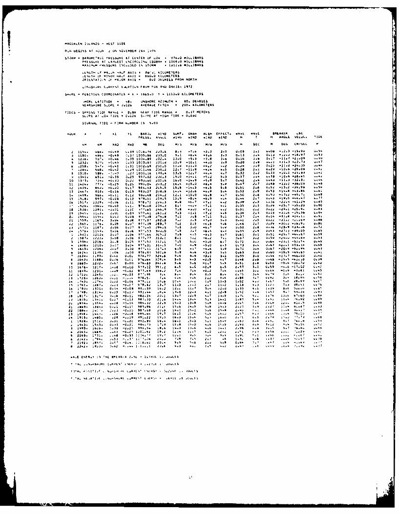
MAGDALEN J LANOS - WEST SIDE

:U1 I.:EGIN5 AT MC)jk d Up, OWL-B:k 26k IFYT 40.

BAROMETRIC PRt!obWR t T LNTE 0 976. 0 MILLIBARS

.Rt "WRE AT A4 f5T LNCIRCLIN [SUSAN IOUS.O MILLIBARS

.A INV. 1MtSSUkL JNC ,DLD IN TURM 1012.0 MILLIBARS

L% Tm F MA ,k MAF AAlb 06C- KILOMETERS,ES T, UF NINON "ALF AX15 960.0 KILOMETERS

JRILNIATIN J MAJOR AA:S 0.0 DtQNEES FROM NORTH

r0iktNT LpuATI N FROM FOX ASO DAVIS, 1972

SHURL - PU41TIQN COORDINATES - A - 1665.0 V - 1110.0 KILOMETERS

,mCRL LATITUDE - So. ONSHORE AZIMVT" - 90. DCUREE5

NEARbMONE SLOPE - J.026 AVERACA FETCH 200. KILOMETERS

TIUf$ - S-RtNG 110t RAN.E 0.56 NkAP TIDE RANQ.L 0.37 METERS

S- PE AT LON TIUL 0.02b SLOPE AT -1(,H TIDE - 0.040

UI RAL TIDE - FCRM N -EIER 15 5.00

.,)OR I Xl VI BARJ SURF. ONSH ALS" EFFECT. WAVE WAVE 6RLAKt a LSC-PRSS : A'N41LSO WINU WIND *INU WIND m I " AN, LL Vt6U1L. VIOL

K4 MAO HAD me DEr M/N M/b M/S. M/b SEC M DEC, CM1btc 01 115- .66. -0.49 -39 Ic".74 2V3.6 S.j -7.6 -3.3 J.U U.00 1.1 U.041 -11.3 -lb.vu U.'.

3 1180. 456. -0.48 0.37 1005.96 2J3.0 9.1 -8.4 -3.6 3.3 0.13 1.4 O.Ij -Id.,) -10.97 V.b3

A 1236. 5UT. -0-6 0.35 100..49 102.. 13.0 -9.3 -3.8 3.6 0.16 1.6 0.17 -11.7 -dl.QV 0.!,0

232. 517. -0.45 .33 1003.b- 201.8 10.9 -10.1 --. 0 3.9 0.40 1.4 U.il -11.3 -d2.7$ -. 7

2se. 5 7. -G..J 0.31 1002.69 201.0 Il.d -11.0 -.. z .. a 0.24 1.9 0.2!p -11.0 -j-.0b

7 i2s.. 566. -0-2 ).29 Iocl..6 2UU.2 12.7 -11.9 -4.4 4.5 0.28 2.1 U.29 -10.6 -25.00 11a 1 30. $68. .. 2T 100 .16 199.6 13.5 -Ii.7 -4.4 4.7 0.32 2.2 0.33 -10.1 -d5.dJ I.-,

, I 1.1. 651. -0.35 0.25 99?.02 dQU.3 15.0 -1..1 -.. a 5.3 0.37 2.4 U.38 -10.610 , 71.. -0.30 5.7 0.42 d.6 U,4j -11.) -ja,)A

.373. 0.12 993.60 dal.6 Ib.Q -14.9 -5.9

1, 404. 777. -0.25 0.2(, 990.0 dQ3.Z 16.4 -15.0 -6.4 5.v 0.47 ?.7 0.4a -14.1 -J6.0.

12 .36. O.J. -U.10 0.17 98b.53 2 ;5.5 15.8 -1..3 -6.8 5.8 0.51 2.0 .54 -13.2 -JV.9b

13 4.7. 903. -0.16 0.15 98 1.27 200.8 14.4 -12.6 -6.9 S.- 0.53 2.9 0.53 -1..*

1. L.99. 966. -0.11 0.12 98Q..6 214.2 Id.1 -10.0 -6.8 .. 7 Q.50 2.0 U.-5U -17,d -45.7 V.69

1: .5we. 997. -O.Qg 0.12 9?9.51 219.5 10.9 -@, -6,9 4. 0.44 2.7 U,%j -19.5 -. 41 -77

I SIT. 1019. -0.06 J.11 9?6.71 id6.3 9.0 -. 7 -7.1 4.2 O.. v d.b 0.36 -dd.. W.05

'526. 1060. -O.U3 .I. 978.Q8 23 .3 8.7 -. 9 -7.1 4.1 0.35 d.3 0.dv -95.7 -sb.dQ Q.90

is 1536. 1,191. -J.01 .IC Y77.65 246.9 7.4 -j.C -7.d 4.d 0.31 d.d U.dd -d9.1 -d5.9.

1, 1 5.5. 11,3. J.Uu 1:U1 911 1 161,1 1.1 -1.1 -1.1 1.1 .. )4 2,3 Ulb -JI.6 -15.36

2, , '':4

5''.. IIS- Q.,3 I. , '"1 7.2 J.6 -7.1 5.1 0.37 d.- U.14 -31.6 -1..11 V.Vj21 , '65. 1.5 -7.0

559. 1. O.U. C.JS 97?.37 d 6 2.8 7.1 S.j 0.41 d.5 U.id -$1.1

1 565. 1176. 0.05 0.0, 97?.39 Zee.? 7.1 2.3 -6.6 5.6 O..b 2.7 U.2v -ju., -db.91 V ::,6

I S?3. 1187. J.O6 Q. ? 29..5 7.3 3.0 -6.7 5.V U.50 2.0 U.36 -10.9 -jj.ub -11

2. 1 576. 11 9. 3." Q.ub 977.53 3 )V.O ?.5 3.7 -6.5 6.j U.5b J.9 U..j -97.j -19.05

Sl- 1210. J.06 97p.b. JC5.2 -5 -6.) b.7 0.61 3.1 U.51 -2S.7 -. 67

I SS?. "fl. O-US ).G* 9'7.77 310.1 8.1 5.d -6.1 1.1 0.b? J.i ul" :11:1 :;1:61.,3 iS96. 1216. 3-9 0.0t 977.53 312.1 1.5 b.0 -5.6 6.7 0.71 4.3 U.b.

, bus. 12io. u..1 0.04 97?.31 31-5 7.Q .. 9 -5.0 6.3 0.73 J.- 0.61 -.1-1 0.41,

1 61S. 12U.. 0.0 0.33 91p.11 317.) 6.% .. ? -... 5.9 0.71 1.. U.67 -90.v -51.9. U.-j

1 62.. 11 9. 1.06 -03 976.9J 310.6 S.9 4.6 -3.0 5.5 0.63 1.9 0.60 -19.1. -V.6!p - .1

16J.. 119). 0-6 0.0d! 976.77 32..6 5.4 4.6 -A.1 %.1 0.55 A.U V.54 -17.7 -. 6.92

8 164). 111@. 0.16 0.('' 976.64 329.4 9.0 4.3 -J.S .. 7 Q..6 a.# ''.40 -. I.uj .:110

v 1660. 1442. .1.0 0 00 VTO 6) 3.1 1.'' '.. U.'' -30.71)

10 1 .ws ':6 , :: -,,, ,, 01 : :11,

'' 1. 12,7. _C:c- §,?:Il 151:! , -0.9 6.5 0.51 S.0 0.59 -. 6 -17.02

1 1231. -9 -C.02 97?.49 350.2 7.4 -0.j 7.4 -65 3.d V.688.1 0.75 -, -':'' U:,

Id 16, .. I -u.03 911.95 J.. 3- a.. 9.5 3.- .. 79 I:v. . I,

1, 026. 126J. .. 11 -.- 916.5. Y.. 9- I.J V.4 0.so 3.7 .Vd J.V 18.96

I. ; I.J. 27.. 0.12 -0.06 9,9.1d 10.6 10. I-d I.y 10.3 1.02 I.L1 5. ea.yV

15 1161. lisp. J.1j -C.01 9,9.62 13.7 11.3 d.7 11.2 1,18 1: l 7*1 11.11 - 1o0al. 0.1. 98-59 16.2 la., 11.7 ).4 11.1)

I '79J. -0.00

a '98. 1114. Q.15 -0.10 951... at,.. 13.0 11.) -. 1 12.0

is I W - 11''. *16 :0 I'l 9 4 10.1 11.7 ,.1 1::5 I.Ju S.1 1.7 J I b1:6U 01, 1 C:l I I I V,

5)5. 131 . C.17 1.6 1..4 IJ.- .87 5.- 1. l

20 1 85.. 1)$.. 1..6 2 1'- ''.0 ).Ve

21 1 869. Ild.. G"! 16.6 1-5 S:t il:,", I:.. b-d? 1.vj

'' I so.. I.:,. 1.., 1'.1 -. o-'' L-

2, "Va. 1.... :10:110, '9.7 Ib.3 15.. :::6 79.1

:1 S., 1-u 1.71 t, 5 IV 11., '7.7$ -. 8

5.1 15.9 -S

19.). 15.3. 0.$3 -0.21 99- 73 iT.9 15.4 15.0

1991. 1 "b. .Jv I..$ lj.b , b 1. 1 %:.1I,9 9! ,, ig'', :Y6 11:11 11,

0.3. 1669. -) , : I a id. 11.7 :c i,:,

... 4 -001 19.1 1 .l .S .. 911.2. ;19 . -53 -L.)* jj '.J. d ., 7.9 ?.5 1., .8

091. 1')1- 1:91L142. INS'. 5:,s 0.8. 3.1 -1?

191Q. ).61 5

,A.E E%[Ry 1% TNE ONLACtR Z %t .1411. Ij JVULES

-211t I JQ-tS

I - -

'AL IE A'I t L %- S L-t Lf-ro - .6- t -b JIQLFS

J

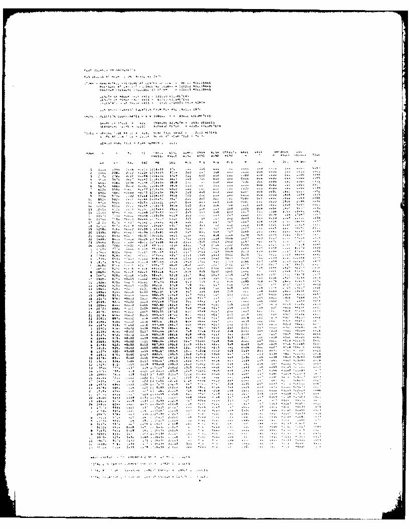
'-42 .4 1' .1 > 11.3 l .1 1 lollU.44043 ,,.

j,54 . '.. A. I, 1 1. 1..44 4> 21

*~~~~~~~ .. o 09 ', )o

1 118 .. 3 5 3'.. D-0 9.. A .. , 3- 9

Os 1.. 008. C..- - 9080432 3. 03 . .0 .. .00

to los: :-8 -. ,2 -. 8349o 3. .0 o2 ,0 . 0

c 507. 1&#. 0.4 -. . t 4 . 4 341.5 5. 0 ..

22 a6AL. 34.-Q-. -.314 .. 19j. . ~ . 01 90

1 .10 . 9. -. 9.. H . 9 ' ' .0 40 ..

26 21335 2.84'. . 2 G& 9 89 too.9 1.5 01.. 04.9 .v 0.d

0 j1449 . 801. . . 34,.3.84 2 .3'. . . .3 1.4 3.0' 2.1 W.; ..

23 150l. la3.. . . . 08 0. . . . . 4 . .

04. ~ ~ ~ ~ ~ ~ ~ 0 .a4 a4-'0 .4 . . . . ' 1;-. 0. . . ..

.30 -4 39 3.. '..1 24

82 3. 11 3' '9 .. 1. . . . .

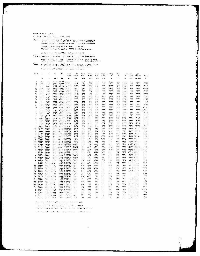
T- - -'t t- 11 -- Wt Al LLNTtK OP LQ.11 LA-L11 Llll"11.1 1 10kil I I- 11LIBARS

1 5TQkM I.A.b -ILLIB-NS

L '"L ''L

-N3S10kt -Rit'.1 L-ATI N L.L.R.C. i ')

t,-ORE ,,SIT!JN CD RCI% TLS 2287.0 l'37- &IL04LTERS

S 0.k AIIT. t . - 1 5. DE NEEI,NEARS-kL Lllt . Q., 37 FL!1. -5.). .1-ftff-b

-IN 'IDL ''A 1.7, ',LA 'j- R VL WtTLN5S- It A' IQ. I It' 35 SL- -* - 3: IV

-. bE Is

A l sL,

A Lu .,b -s -s M 5L, DL.

1-5 IjA.87 n.

"Am no1 1..'' '1.!

31.5

3"1 7111jo@ -1.1. "Am 32

'a W. IV- -'',I

1011 R23 1193. 125- -v -W "Am K

IV

111$5. 15c.. a.il 37 o

:.O 1-'': 11 o I., 3 'I " * 11 1*1 1,15 .s I.j I.. I" I..

117.. 1.13 -G.29 LQ16.11 1 - Io.e. ..&$. .. Ij n 7 w 12

1461. .is I2Q 3. I.S5. 0.13 -0.22 101,.51 3..Z O I

1:' ! a : a W a a a :j

.1 10". 1 36. .'j to a a 0 ; : a Q a a a : a R a 1 a any P, Ill. 1.2s. ''.1321 1138. 1.1 . ... :.,: 4 TON I A ! A A 1 A : A 2 2 11 29 t V=Z 21".11* *11: 1 11 -0.0 111-6 1 1.1 1 1:1 1 tI o -0'.

: I

I.o'1. . 11. !so.. .13 5.1 .Ub 1:11 1. 111.1:01 11 .1 11-1:'

di.j. ije.. c.i. -4 11

:111 13 1: ':13 1.1, 1-11.1V I:. it

T Lou 1 A 1 v 1 1 0 1^.I.

ON

.1,11-: :1o; ''I'

:Z:1 0:!

.11 Lis it 1 n I A 40

4.... Ile- -,.,eIjLj..' 's'..

o''3 V.'

ei 1-1,

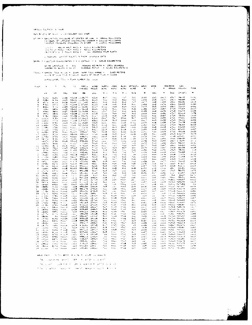
A... IjA2 I I..v.A

'4..'. ~ ~ ~ W '4; 01'. '.. .-. 3144 i. a

32 4.- 5 .~'.- ..-56 S.. t% It74 L 4 . 2. * 4.v 1..i5

Sb., .. a. A3t7. *% wIjs. ;...4t744

*i- A .'.. A.!.L .o ., 2454t 4..M 52

- .. 31- L .- 7. 4-'' 5 7 .* .L. 1fl31 ,

543, -~41.. j..%A745 I . -~. 525.0 6440436 7('4

I. ,4 .. 7.-4 * 14. .786424 A274.74 290. W04.Etb6

-. tbA .5 ,. 6-4 .. i 4.A MAv i 4 Fk .7 3 y 4o.L..v4614'

-74SS. AL..4 .II a!. I 2. s"L; SL ND 3' SN2 44. t . I7I 6

* '.'.. . 2.U . I:.' t. 7. 71 .. 1 I u. 7 dfl ,8~ *.s

3:2 S0:. 5.. 2'3 4' -7 . .0 ... 9

* 4 * . 7 - -'.1 ~ * ~ 4 1.7 .4 .. 2 4 4 3 3 . ' . 2 .. 4 .49 :. W

- 48. :. -. 2 -v42 '474 .' ~ 7 .3 77 .5 v5

4.73 f7.1 -.

.20.22. 1 . 41 1., 1.06 374 '. 4 v2

.3 243. 7').2322w 4.5 .. 7 4.. .v.4 .,. .. / 4. 2.' 3.3 7.A4 4.2

..- n. ,'3. , .. 4 ~39.3 :. 07~' .' .421 7.4.5 v4

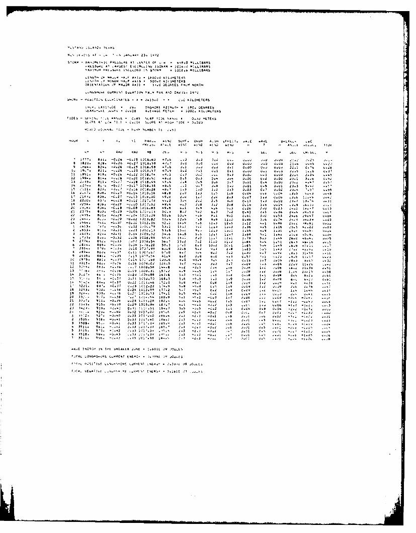
k.,. tiN '. .NS XN,.Vl 23 . 70?

STORM - AK2867'.IC FA'.OSuRE AT .6NTERGOF V9'.8.0 Rja.I8ARS6

AXIo Vt ~ I- L o L o2 0 D 76 1. 10180 R ILL.8As

.EN.5T 06 VIA...) 'A..F Aol.61 II : , 180. iLOME TtS5

'"O'. "10 . ... AXS 00.0 KILOMETERQAIENTAT1l05 FNMA4

038 AVIS 31.0 0(06665 PF'soM NORTH

,ONy75S"0'.k CVRNIN E.'.,ATION 60.9t FOX AND DAVIS. 191d

bHORt - VsOOI7I.N C0,.VINAIES - A - 0.16.0 Y - 0.0 KILOMETERS

Im.XL ATJT7C' 28. ONSHORE AZIRO T, 200: DEGREES, ELAR!'-..L .LO0 1 0 ;. AVE 48 FELa t000.) KI L 386TER5

TIDES - czl% :.!, %AL. .6 AP tI). .A%,I 0.30 678388

Ss26E A:" T2 . k s. .>'I S.086 AT IGi. 'I1 0 00

OV A ' 1 FARs. I11 SOVF. 0458 A,5" LEVEL!. oA.E SAVE 08.... ..aA3,5 A'.LE .17. .1"0 .151 ND2 H 7 a A0 ~ I..0. 10

6 120 BA. -026 -027106.9 '.. 0. 0. 00 . 0.00) 1.0 Q5 021. t, 4 00.'X. 8'. 0.6 023116.56 '.7.B 01 0. 0 01 0.00 o.s0 0.00 22.1 078 .A

1,. 111. 601 O -!.23 .136T~ .9 0.2 -1 0 . 0.1 0.0 .1 ii00. 1-. 0311 I I81 II.00o 2 101.5'. .8.1 0.3 . 0. D. 0.0 sal 0.0 u 0. o.' I ..12 '99.. 61. ' 6 -. 011.0 .. . . . . 000 V.0 03. 3 ..0013$ B lI.. -. 07 -C.20 1318.46 '.8.4 2 . 0.0 . 6 0. 0.01 0.'. 00,70 T 00I 211 1 80. 70. -0.1 1182 '.7 3 1 .0 1 .1 13 00 0.7 0.00 23..1)2.6

17 13, 80. 227 0.1 108.0 '..0 . .7 .. a 0.07.)0 1.0 0 .3.'. 1... oX

19 ~ : 0'Olda 02 2.011730 '84 . .3.8 01 1. 1o1' .0. IX. ,.

1 1037. 603. -00 00 Os. 3. . . . . 0 0a7 3.2.. s4.0o -5522 i'.7,. 901. -2.29 -<.34! 10 :9 6. 10 '6.6 8.1 4.1 0.01 3.0 V .U 0 .' 9.? 0013 ZI'... 8.0 .2 -0.00 1013.82D 31.' .1.6 1.8 9.8 10.0 0.8 3. 0.I 2'.' 3 .3 .3

1 05. 37 -. 3 10 1 719 63.1 163 30 1a 3 13 1. 1 206 '.0 00

3 8 3 . 3 2 . - 0 3 1 3 0 4 1 0 9 3 I' . b' . 8 ' 1 2 1 . 7 1 . 6 0 . 1 .4 .5 .A . . .

5 07'. 66. -. 33 2.0 133.6 667 1.2 . 1 1. 110 0.6 6.4 1 .61 06 '.8.6 .6 81 .66.c.' 001. 0 683 1', 10. 1:.1 1.6 2.4 1.49 26.8 -. 1 11.

9~~~~~ 0333 881 -263 a.1 l0'1 31. 6.1. 60 0.6 7. .f '.8 1.7 s11 305 88. -. 6 01 101380 50.6 32.7b 0. . 1 . 0 .83 1.3 0.8 0.' 1

d355.,. 0d. -2.76l -0.13 l12.31 1602 '.,9 -a.6o i, 1. 1.7 .0 1., 0.8 25.9 10.26 1.0810 3: ;* -. 7 02 007 18.3 6.6 -0.6 1 .1 1,.9 1.3b 1.5 0.06 6'. 5 4-22 0.'.

16 ~ 1 1>2 83'. -03 02 1 .. 17. 0. d0. 0. 1. 5 .. .v 1.31 .15- . 3' -4,

I 3 0 1 8 3 I -0 .3 7 0 . 1 0 :0 .2 1 7 . 5 . -0 . 0 . 1 9 0 .0 ' . : , 1. o .: 0 . 5 1 . 7 816 303. 40. .. 8 0 102 .99 7. . . . 1. 0.1 1.0 41 1.' ' ~ .i196,-. 0. -0.7 . 2 1.7 170. 6. -0. 0.2. 0.9 1, s. .. 0. .o20 33. 32 3-7 LC 012' 4 1 8. 1 II.1 -2.0 1. .4 1. , : .o

21 37 ' 1. -03Se826.9 1 0 '. -0 . 1.0 10 00 . s0 -.1..', .

2--.. 93-.. .32o 101.0 185 0. -0.31 -0. 0j b 20 0. 1.Q -2. -1.30 I

3S 36 5. -. 2 03 1d'. 16.:0 6.3:7 . -. .8 .1 II5 <.0 sIo -4 ~ ~ ~ ~ ~ ~ ~ ~ ~ ~ ~ b 351 96.1.0 08 073 87' 23 -. 00 o8 0 0.1 -l' -. ' a 5 .

7 32. 96 2. , 10 '.3 18. ':.7 -0. - . 3.s . U., -,'- . . .

02G.6 L0900.J'5 CsVRN (5060y 7.79 V s

T< IV6!l E 03 0 2A <00.5 LN'' *. -.39< 09. 1Loo'I

17. 3 fs.71. 0 3>-'0 1.884 75680 *U 2..61 022 -

11 1-,:1:6 1:5 :1 : I~b 1: ')" I :. "

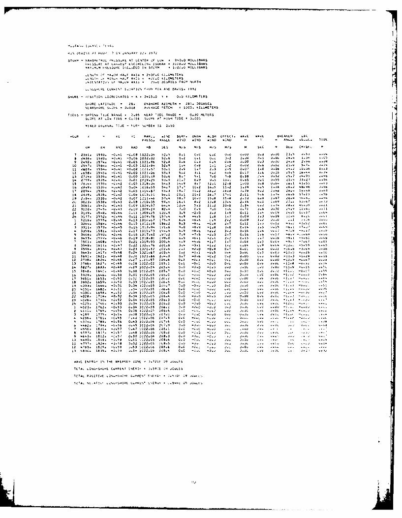
wi0% 4410I\S AT 00400 7 ON OANUARY 1.. 1'.10

STOQ. - 4ADtTNIC K,5S9L AT LENTER OF LU. . 940.0 MILLIBARSHLSSAE AT 4A',EST ENCIRLI. N ISOA8AX 1018.0 MILLI8ARS

'AXmIH L w4O I-LtODED IN STORM * 022. MILLIBARS

Lt kT" C' JAoOA HALF AXIS * 2500.0 KILOMETERS

NUT-' .F MI\'. 'ALF AX10 * 4Q'0 ILOMETERSRIt9ATJUI oF 'A )V. Ax1I s Z5.0 D E EES FROM NORTH

L.045(60RE L09L 71 EXAT ILN 190M FOX AND DAVIS. 1972

SHORE - POSITION OOR0IATES - X * 2X15.0 Y 0.0 KILOMETERS

SHORE LATITUDE * 28. ONSHORE AZIMUTH 280. DEGREESNEARS HRL SLO)PL * 0.018 AvERAE FETCH * 1000. KILOMETERS

TIOES - SPAINS TIlU RANGE * .85 NEAP TIDL RANGE 0.30C METERSSLOPE AT LO. TILE I t01E SLOPE AT HIGH TIDE . 3.D20

MIXED DIURNAL TIDE - 0Rl NUMBER 15 2.50

HOR X XI Y1 RARO, WIND SURF. ONNH ALSH EFFECT, WAVE WAVE AKLAk LbCPRES S ANGLE WIND WIND WIND MIND H T ANNL XEC. TIDE

M M RAO RAD MB DES MiS M/$ M/S M/ M SEC M DL. CM/tL H

7 2381. 1593. -0.41 -0.08 1022"04 52.5 01 0.0 X.0 0.0 0DOl V.A V00 03.0 o.57 X XN

8 2430. 1583. -0.41 -0.06 1022.02 52.6 3.0 0.1 0.. 0.2 3.00 3.1 V.OU jX,4 1.3 o.O5

9 2 4 . 15W. -0.41 -0,05 1001.96 52.8 0.6 0.2 0.5 0.b 2.0D 0.3 0.00 2'.b 2.Xt V eU.10 2547. 156'. -.2.X -0.03 1021.8' 52.9 1.4 0o. 1.1 1.2 0.02 0.6 0.02 05.v U.0. G.1III 2603. 1554. -0.41 -0.02 102151 53.1 2.9 1.7 2 3 2.5 0.01 1.D 0.26 '.,0 10.6 U.3

02 6R 155. U -041 D0 1D21.0o 53.3 5. 3.1 4. '.5 0.11 1.6 .1? 5 16. XA3

13 271. 1535. -0.41 .OD 1020.19 53.6 A.7 5.1 70 7.6 0.38 0. 0.32 5.7 oX.95 ,

1 2759. 1835. -0.01 0.1 29.25 53.9 11.7 4.9 9.5 10.1 0.65 1 .b 55 .5.9 33.2 T *.515 2 04. 1535. 0-2 0.03 1318.' 5.3 14.9 8.7 12.1 12.8 1.00 3.8 0.8.t (*,I 41.S5 '.6

16 Z8.9. 1535. -U.42 0 04T 10.2 1.S 1S.2 1.39 16. 5.5 1 AS 4.8.96 -X617 2894. 153S. -0.42 0.5 121 .8 55 . 1 9? 11.2 16.0 10.8 1 7A 5.2 24 2.- 5..b. '..3

I 2939. 1535. -0.42 0.06 1013.11 SX.1 20.1 11.0 16. 7 17.1 2.11 5.6 1.74 26.6 51.05 *St19 2)84. 1535. -0.42 01 1211.46 51.4 18.1 10.0 15. 15.8 2.3u .0 I.A 26.M 06.8. X.'.21 3023. 1538. -0.43 0.08 1010.35 59.X I.1 8.2 13.8 13.4 2.38 b.1 1.09 276 53.67 '. I21 3061. 15.2. -0.43 0.09 1009.57 64.4 12.4 5.3 11:2 10.0 2.34 6.0 1.7. , ,.0 21-22 3100. 1.5. D -0.43 0.Iu 1009.19 82.4 7. 0.9 70 5U 0.11 3.6 U.30 1., 12.b , '.23 3139. 15-8. -0.44 0.11 1309.25 12U.9 3.9 -2.0 3.3 1.9 0.11 1' V,09 .IS I..37 .. *0-

24 31T7. 1552. -0.44 0.12 1009.76 157.4 4.9 -4. 5 1.8 1.7 0.09 1.3 U0.9 ICt 8. 2. -11 3216. 1555. -0.44 0.13 1012.67 V75.8 6.6 -6.8 2.' 2.2 0.89 1.2 O. '..1 .O L*V.

2 126. 1564. -0.44 0.15 1012.19 166.2 8.3 '8.. -0.8 2.7 0.12 1.7 0.1 2 '. 2 3.50 :'.A3 3311. 1573. -0.45 0.16 1013.94 IVI.6 9.0 -d.9 -1.8 3.0 01 4 1.5 0.15 -.6. -71.. LL'

3358. 15,1. -2.'5 0.17 1015.13 15.9V 8.9 -8.6 -. 2 3.2 0.16 1*6 A? -7.8 -4..7 .1...5 3406. 1590. -).46 0.16 101710 .97:2 7.9 -7.5 -23 2.7 0.16 iI 1.6 -. ,.bH :616 3.51. 1599. -0.46 0.19 1018.81 199.0 1 -1 -2.1 2.2 0.15 1, * UIt -9.1 -_.6b U.b1 3501. 1608. -2.47 3.21 1019.93 200. ' -9 -4.6 -. 17 1.7 0.D 1.3 0.0 -.9.7 -7.6 _*V58 35'8. 1611. -0.47 2.22 1024.76 201.6 3. 4 -3. -1.2 1.2 UU, U.9 UA.0 -10- -5.S 4U.I

9 3596. 1614. -0:47 0.23 1021.32 0.6 2.1 -2.0 -0.8 0.7 0.01 0.6 .I -1.. -3.60 .,.7

ID 36.3. 1617. -0.48 0 2 : 1.7 ,03.4 1.2 -1.1 -. 5 U. OUO 0.3 UU -11.0 -6.26 '.Lj11 3691. 1621. -0.8 0.2b 1021.86 224.0 0.1 -0.6 -0.2 0.2 0.00 9.1 0 .0 -11.3 -1.26 U.,I12 3 38. 1626. -0.4 0.27 1 L21.97 234.6 0.3 -0.3 -0.1 0.0 a 2.00 -.A 0.00 11.5 -U.

7 .cX

13 3786. 1627. -0.49 0.28 1322.02 205.1 0.1 -0.1 '.0O 0.0 o 0. Ul -l -11 .8j

a' 3427. 1633. -0.46 0.39 1022.04 203.' 0.0 -2.0 -02 0 0 0.00 .00 -11 ..- 0*16 4,115 38,8. 1640. -1.48) 0.30 1022.0 005., 0 0 0-. - 0 D0 00 0 2.': u0 '.0. : .016 3909. 1646. -0.50 0.31 102305 200 0.0 -0 0 0 0 U . 04 a'Q- O 1i o .

17 3951. 1653. -0.50 0.30 1.22205 026.2 O. -0.0 -).0 0.0 0.00 . 0. 10- h.-. ,. '18 3992. 1659. -2.50 0.33 1020.05 206.5 7.0 -' , -0.0 0.2 0. . . .. . . ....

19 .033. 1666. -2.51 0.54 1022,OS 206.7 3.0 -0.0 -. 0 0.U c .vO20 4031. 1682. -2.51 C.3. 1022.05 206.6 0.. 0 -0. -u. U .0 2.0U U. . U . .- . .21 4030. 1698'. -52 0.4 1022.05 206.5 0.0 -0.0 -o.U - . .00 .j4.X0u 2.4.-.- o-.,7

22 '028. 1714. -0.52 0.36 1022.05 206.4 0.0 -0.0 -0.3 U.0 O.U 0.0 J,.. - 2.. -- ,23 4026. 1130. -2.52 0.34 1022.05 20 6. 3 0 -0.0 * 40 00 4.0 0,. --. s --L. I - 0)2' '. '5I .-2353 0.34 1022.05 206.0 0.0 -2.0 -0.3 0.0 .1 0- - - - -- - ,- - -

1 4023. 1762. -0.53 0.34 1022.05 206.1 0 -2.0 -0.0 0.2 0 .2 4.04 - , -0

2 4 111. 1769. -0.4 0.36 1322.0o 006.6 2.0 - - 2 U4. 2.00 ", L* -, . . . .3 4199 171. 0.5' 0.38 1022.05 201.0 0.0 0.0 "v.0 0.0 0 7. U -.. . . .I

4429'6. 1781. 0 -25 '.40 1022.06 2 07.3 0.01 U -0 '.o 14 0 . 44'.. 1.05 437. 18.. -0.56 0.43 1022.06 2o7

.6 0.0 -.0. . . .. 0.. .:.V .

A 4662 17 -0.6 0.' 1022.0 ,0. 30 '.2.4 -4.0 u- '~0 . 44 ,4 - -

1 4'580. 1831. -'..5 7 0.47 1322.06 1'A. 3.2 -0 -U. 0

L:, .4 .. . .

a 4597. 1837. -0.5' 0.48 1022.26 00 8.2 0.0 .0.3 .. 0.I I o9 4643. 1812. -2.57 0.50 1022.OM 208.3 0.01 -3.2 ..o .1 .0 2. . . . .

10 6690. I818. -0'.58 0.51 1222.06 206.4 0,0

-0., -0.o 0 .. 0.0- - - - - - - - - -. 411 .7317 2. -2.58 02122.06 @0.-1 0.0 -u '.2 02 004 2 ., 3,12 .783. j8@9. -0,9 .. 53 10222.0 200.6 0.0 -0.2 -. *. v.u 2.00 *

3 4830. 1835. -0.9 0.5. 1022.06 208. 0..0 u -3.0 0.4 0. -. 1.04 -,. 2. ,

WAVE ENERGY 1N THE bREAKER LONE ) 721t 09 JOULES

TOTAL LONG-SHONE CURRENT LNEAS' * 0.59JE 04 JOOLES

TOTAL PQSITIVE 42N-.E LCAENT ENEG3 * 2.Sq0t 29 9 ,

T0744 N A7

" 1 4N0.S,3RE .TE.E 05 2 S

27

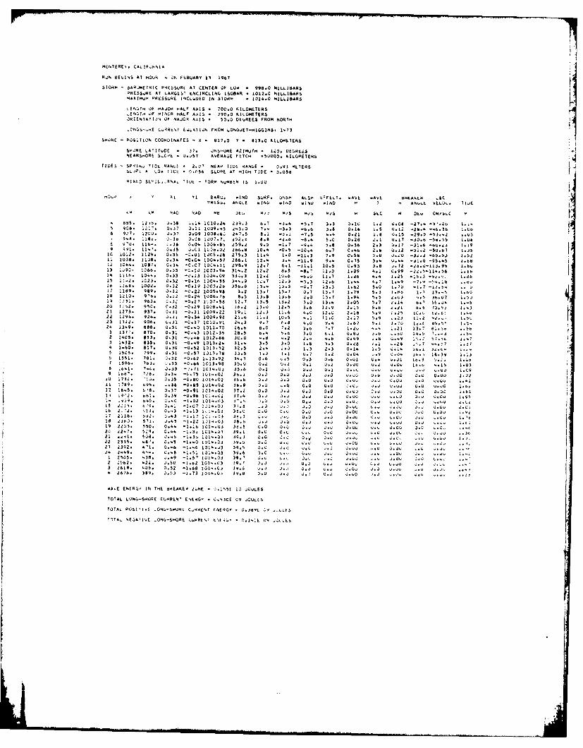
MONTEREY. CALIFO RNIA

RUN BEI S AT HOUR 4 ON FEBUARY 13 1967

STORM - BARJMETRIC PRESURE At CENTER OF LOW * 996.0 MILLIBARS

PRESSURE AT LARGEST ENCINRCLING ISOBAR * 1012.0 MILLIBARS

MAXIMUM PRESSUE INC41.EO IN STORM •1014.0 MILLIBARS

LENOTH OF -A2ON HALF AXIS * 700.0 KILOMETERSf70 TH ') F vINOR hALF AAIS * 390.0 AILOMETERS

ORIENTATIN OF MAJOR AXIS 50.0 DEGREES FROM NORTH I'

.DNG- o CORRLNT E UATION FROM LONGUET-HIGGINS 173

SmORE - POSITION COORDINATES - X * 817.0 Y * 613.0 KILOMETERS

SHORE LATITUDE - 3T. N0RE AZIMUTH * 1 O, DEGREESNEARSNORE GDL 0.057 AVERAOE FETCH .5000. KILOMETERS

TIDES SPRIN, TICE RAN~. * 2.07 NoAP TID RANGE * 0.91 METERS

SLOPE A' LO. TIDE * 0.75b SLOWE AT HIGH T;DE * 3.05b

MlXO SLIL,.RNAL TIDE - FORM NMB0R IS 1.20

H4 * 01 '1 BARD. HIND SURF. ONSH ALSI EFFEOT. WAVE *AVE dOtA.4 ,.CPRs . ANGLE wIND wINO W 140 h T H ANUL V EOL. IDE

KM OH AD HAD b7 072 ."3 9/5 47/b M/S A .C H DER CR/AoC H

1185. 1. 3.36 1 4 :1102 23.J3 6.7 -3.4 -5.7 3.3 3.Su 1:2 v.08~ -2'..:: 0 1.5 38* 131. 0.37 3.11 1009.45 2.3. 0 '' -3.3 -4. 3.8 0.16 1.5 0.12 -28.4 -'4.3 6 3 .& 927. 1200. J:37 0.09 1008.60 247.5 8.1 -3.0 -71 5 0.21 1.8 0.15 -29.5 -53.42 s.Uo

98. 1182. 0.34 0.08 5307.7. 192.4 8.2 b.4 -8.4 5.0 0.28 2.1 U.17 -30.6 -5 ..5 180'. 16. 23 0. 10345 259.21 9.0 -1. 7 -W:4 :.8 0.38 2.3 0:13 -1.6 60 , 119 59. 114'. 3.35 3.01 IC-36.8O 266.8 104 -0.5 -10.4 6.7 0.46 2.6 5.12 -30.2 -50.87 1.3

10 1012. 1129. 0.35 -3.01 1005.25 275.3 11.4 1.0 -11.3 7.9 0.58 3.. I. a -1..2 -85.51 1 °5212 1038. 1138. 0.34 ".04 1004.57 286.1 12.4 3.4 -11.9 9.4 0.76 3. 4.4 -W .0 -9.4 1._b12 1064. 1087. 0.3, -0.07 100 4.11 299.9 12.7 6.1 -11.1 10.6 0.93 3.8 U.72 -2I.b-113.99 1.6013 1490. 1066. 0.33 -0.J 1 003.94 314.2 12.2 8. -8. 1.0 1.09 4.2 I.99 -2.9-114.6 1.614 1116. 1044. 0.33 -0.13 1034.09 330.3 12.2 10.6 .U 11.7 1.26 a .4 1.25 -15.3 -I. 1.8615 11-2. 1C23. 0.32 0 1 0004.55 3 4.9 1z.7 12.3 3.3 12.6 1.44 .7 1.49 -7.9 -54.iR 1.9016 0108. 1002. 0.32 -0.19 1005.26 356.8 13.4 13.3 -2.7 13.3 1.62 5.0 1.70 -1.3 -1.54 1.1? 1189. 989. 0.32 L0.22 1005.98 3.2 13.7 13.7 0.7 13.7 1.79 5.3 1.58 1.7 13.-S 1.6018 I010. 97b. 3.-2 "0.24 10076.76 85 13.8 13.6 2.0 13.7 1.94 5.5 .U3 .S '.07 1.I09 :231. 963. 1. -0.27 I07.58 12.7 13.5 13.2 3.0 13.4 2.05 5. 7 .J4 L.41520 1.2. 953. 0.32 -0.29 1008.41 16.2 13.01 12. 3.6 12.9 2.13 5. 2.21 6 5 70.53 I.'21 1273. 937. 0.31 -0.30 1009.22 19.1 12.3 11. 12.0 2,18 59 25 1. 0 I.22 1294. 92. 0.3i -0.34 1009.98 21.6 11.3 15 '.1 11.0 2.17 S.9 0.23 11.2 .2 ; 1.-23 1322. 906. o.31 -0.37 1010.91 24.3 9.7 l8 4 0 9.' 1.67 1.1 1.70 1. v. 1.-24 1349. 888 0. 31 -0.40 1011.70 26.6 8.0 7.2 .0 717 1.2U 4.4 .21 13.7 b.4, 1.54

1 137 870. 0.31 -0.43 1012.35 26.5 6.4 9.6 3.0 4.1 Q 8U b. .H 14.5 7.-3 1.5.2 10. 833. 0.31 -. 46 1012.88 300 4.O. 2.4 '4.6 0.4 9 '.8 Q..9 15.2 00 14

3 1 4 30 35. 0:31 -0.9 10 13. 2 31.4:1 3. 3.0 1 . 3.3 2.28 2.1 -. 28 jo.] 4.57 . , I :4 14e6 817 0.30 -0.52 1013.52 32.5 2.' 2.3 1.3 2.3 0.14 1.5 0.14 14.1,. 1..

5 1505. 799. 0.31 -0.57 101'.78 32.5 I.3 1.1 0.71 1. 0.0 . 0.04 10, 18.39 1.136 1551. 781. 0.32 :0:62 1013.92 34.3 0.6 c.5 0 3 0.8 O.21 0.4 4.01 10.3 '..i I.o

1596. 763. 3.33 -0.66 1013.96 35.0 0.2 0.2 0.1 2.2 0.0 0 2.1 0,2 14.W 4.19 1:038 o 1 9 . 0.33 -' 71 1314.01 35.6 0.1 2.0 0. .u 0.44 2.04.02 !.09

10 1732. " 10 0.35 -0.8 1014.02 3b.6 0.0 o.0 0.0 2.0 U.4v ).v U.02 Q.0 O.. I.'111 189. .. . 0 ,: 1014,32 36,9 0.0 . 0 0. o .. 000 2.20 U , 1.4,

12 0845. S8. 0.37 -0.41 101402 37.2 00. 0 . 0 .0 0.20 .2, 0.00 0.0 0.00 0.1,iA-'2. T 6. 0.39 -0.96 101'.. 37.4 0 . 0 0. 0.2 .2 0.0 . O 0 . 01.02 ,.95

b' 4; 9. 44S. 2.40 -1.02 l1.0 03 r.S .1 0.0 0.0 .0 0.0 0.4 o.2, 0.20 .U I,IT 1219. 92q. 3 -1.07 11.03 37.9 .3 1.3 0.0 0.0 0.44 4., C.,L 0.- 0Ov Q-.0.

16 22. 431 0. ) -1. 241 .03 38.0 0.0 0U 0.0 0.0 0.00 0.. 0.00 .0 4.34 .42IT 1 211. S29. l.3 -0.1 .. 3U 9.3 0.4 0.0 0.0 0.0 3.04 2,4 v.21 o.0 0.04 1. 521 013. 57. 0.43 1.20 1314.43 38.0 3.4 0. . ,. 0.4,0.44.2 0.0 4.0,2.7219 203. 550. 0.43 -1.2 101.03 39.8 0.0 0.1 0.. 0.2 ,0. 0.L 2.01 0.0 4.0 .20 127 509 .4 -1 04. 03Q 39.e . ~ 0.4 0.0j 0.0,Q U.2 0.0L 0. 0.4 ,

21 321 0. 0 .4 1 1. 30 1314.0 39.3 0.0 30 0. 0.0 40 1.1 UU,. 0. ., 1-7.22 2395 1 *8'. 0.45 -1.*0 1014.13 39.9 0.0 2.0 0.0 4.3 2.04 4 . . 2..0 3.21 09. '1 .46 _I. 01.43 39. 0.0 0.4 40 2. .0 4 :.20. U .. L :,. .24 2335. 4 1 0.8 -15 1014.03 39.65 . .- 04 02 04o ,~12 . 42 24

13290. 431. 0.49 .5 1043 39 .' 3.0 o. U. Q .. 3 1.4 . 04, 2U U.4...2 2562. 2. 0.50 -1.62 101'.33 39.' 33 , u.30 .4 o.. .2 2. .6 2 .)3 2619. 43S. 0.52 -1.6 1014.03 39.9 0.2 3.u 0.0 4.4 0.0 -v.0 2.01

4287b 389. .53 -1.73 1014.0, 39.8 3.0 4.0 0.3 0.4 0.44 ).0 .W U ,. .u ,. .3,

WA.E ENEAGY IN THE dREAER ZONE * ').IS5E 10 34LE6

TOTAL LONG-SHORE CURRENT ENERGY * 0,530E 09 JOULES

TOIAL P OSITI, LONG-SmO00 CR9ENT ENErgY 0 .39 9L L9 -LtS

T7T NEGATIVE LONG-S9ORE L4RE OE'.L . 0.1NIE 04 JOUIES

tI

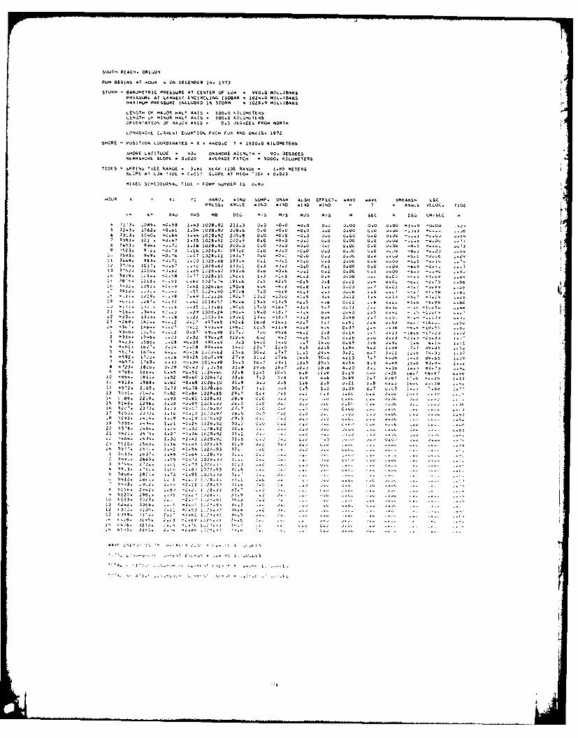
SOQTH BEACH. OREGON

RUN BECIA95 AT HOUR ON DECEMBER 14. 1973

STORM - BAROMETRIC PRESSURE AT CENTER OF LOW - 990.0 MILLIBARS itPRESSURLPAT LARGEST ENCIRCLING 1 508 AR : 1024:0 M LL BARSAXIMUM k IS, SURE IN C LUD E D I N STORM 1 028 9 M ILL BARS

Ir

LENGTH OF MAJOR HALF AXIS - 500:0 k LQM ETERSLENG 7 m L M I NOR HALF AXIS - 500 0 K LQ ETERS

4,A I, AJOR AXIS . 0.0 )LGNEES FROM NORTH

LONGS"OHL COR-RkNT EmUATION FROM FOX AND UAV15, 1972

SHORE - POSITION COORDINATES - A . 4400.0 y - 1520.0 KILOMETERS

.s"OR E LATITUDE - 43. ONSHORE A214UTH - 90. DEGREESNEARS H 0 , i SLOPE - 0.020 AVERAGE FETCH - 5000. KI LUMETERS

TIDES - SPRINU T I E.kANQE : 3*,"l NLAPIIOL.RAIIIE,;, 1:.11,11ETERSSLOPE AT LO TIUE " 7 SLOP T IQH T . 0 2

.IXEL SEMIDIIJRNAL TIDE - FORM NUMBER IS 0.90

.,)UR I y Ai YI SA SURF. DNS" ALSH EFFLCT. WAVE t1KEAKLk LSCRe- !No IND WIND WIN;) WIND H I ANVLL VLL(J(.PRLSS. A .LE H TILL

KM R-p RAD Ms DEG M/S M/S M/S M/S M SEC M otlo cml$kc m

I-3 1085: ,:4.1 101::91 211:1 0:0 :0:1) :0:1) O:U 0:01) 0:0 U:OQ : I::, :11: 1WJ21": 0

5 02 92 2U8 6 0 0 0 0 0 0 v 1) 0 uO

3 2 0 64

6 4 O ,.92 3,.a U.0 0.0 ).o U.0 O.Qu U.Q U )U U7 1381. 1 0 1 U .. 7 3 0. 92 0.0 0.0 ).a 0.0 0.00 0.0 -ow -11, :7 1a 3 , 53. , 9.. -,.7J 1. 2 6 1 02 @. 12 11 3 0 u u 0 1 0 1) ou 0 0 U .OU -9. _U. J. W 71. 6 1 8. 1 7.0 , .') I . -0.

23. - .') 9 0 0 C 0 u A) J Q .19 U 1 '2 ' ; . o -0 c o . Q u . u u . iv.9. - .76 1.07 1026.31 193.7 1., 1 -1.u63'.9. 63. -0.71 1. 0 1 ,.uVc J28:11 1133:4 : l 1.1. 1.0 O.U 1.11U U.11 1 -1:1 -1:11 :.7

!I 31o . 101'. -. 7 9 028 82 1 1 1 _U.. , , i 1 0 0 n 1 0 uO L) 0 -6 5 -Q1 2. 6 D C b u I U.D

1., 1.1 L.1 L . 4 Ou. 000 D'U,19 "1" 1 .!, , " 1. 2 ., 2 .5 _ 0 .5 U .8 V . j 7 ,U, 11 4. U.,

-2 1 .. , I .. 4 1 11 1 1 0 031% 393". 1.11 1"224.90 99-: 7.D 6 .9 _ I .3 1., 1) . 06 1.0 5.1 56: ,ji: 12Z9 -3 b.7

zv2 :2. 19J:? 1,):2 -10:0 3 0 12 1.-

I I 1 :1:9

13.0 :13.5

19 1 16 I 17 90 1 d 5 :b 0-1 1.0 U-1 -b,7 7 J . I5.7 2.1 u.j,

0.40 j:1 :,7

1 2 -23- 1 3j). -,.,b C.22 . 2.14 I U.j 11. -111.7 -,.j b.. 0 .8 2 72 '269. -l.12 .1? 49 7 ., 5 1 91 .1 1 6 U _I.3 1 4:,' C.,37

I

4 43 7. 1'643.6. -1: :L" 2V". I.G -1.96 -1 1 2.a U.11 I.1 U.132 43J- 15 6. :-'3 1: l 91, 311. 11.1 4 .3 1-3. .58- " :,1 4 0 L: " ':U J:'3.. C a L 99 19 1.0 14.1 14. 1. 1 14 U 0 a, 1 6 0 1.- 1. 1.2'. , - . 3 .. 1.. 22.' 2 1.9. 5.2 1.90 ;.1 1,J

45,1. Ib'- 3", ,, Ijo-ba Z3.6 30. i .o 14.1 11.4 3 2, 6 7 21 377 1 9 .27 31.2 27. 14. 30 1) 4 13 7:7 4:,)*b57 17": )4 IQUI:99 4,9 0:25 01. 811 1 31.V3 2t.? 1 13.6 5 5 4 54 8 3z ':'6 0:39 -C..3 .11.8 J9,& jb., 10.3 1 8.6 4.,eO 4.1 -7,

4 4 1 1.2b i52 1 61 0 L). I : : 2,13:1 17:, :, b:, ":9I J. 1966. J 0 a J 2 .1 I., 3 .u 1 .1 1. 6 1 .1 u 1 1.8 0.11 1- -3 1

I 1 1 9 6 6 U 19 1 1 712 4S 2. 2LGS. 0.72 -0.7 , Ic,24.66 0.7 1 .1 0.9 t.s 1 C 0.03 o.7 L.0 1,4. 1.6.13 5031. ' 42. C .8 2 0 . 1020:895 29:7 0:3 :3 1) J:OU o:2 v: , 1

14 ,, 89. 2219. _9 .:j ) 28 9 1) 0 Uu15 5118. 2 96. .J 1 2- 3 0:1 1:0 1:11 L.,1b 052c' 23?3. 1.1 C7 I U L 0 U, u17 5 5 Z 13. I.Jb 1 21.92 2,,. J -L,,.6 529 J. i 1 .,8.92 29.3 0 : ' ' - ,

5. ":: 1 1 2 i - u L L L19 533 ill I I'1 .91 :'9 '9 ': ' ':L -',

4 ,11'1: :1" !,.::12 3c. J: J: J.,: 1 7 :1:3

f _1 3b I I 1 31. , j -u1- 4 1. 1. , I.

3 1 . 41 1, 9;'20. 25,3. 1.36 -1.19 IJ28. ' 31.9 .1 Iui 55 ". ZS;_. I..Z _1.5 6 IV 2 a .93 32., -

1111: 1631: 1:11 1,11 3 3Z.1 1: J7 U

7

5 5666. 2821. 1.73 1 31

593J,. 9 j1- - 2

q12. 1.01

3 .931.1

12 ,3jw-1 1319: "I'li: 11.114 1 J.,u:111 L1 6. 2 , " .

15. 3i .. -2.6,

14- L 1'1'

T

T' I A, T

T A,

:14

C~~ ~ .',A U< t-

-b :'> 7 *,IN E

LM< -,4TU J '25 ,,i>. - .

3,<U Mb 22 ~ ' >

2.21 2 .5 .. . --. -. . .L

<5 0

18.. .1i 7 - ~ 2<

2 i . -

L L3

1 11

3L,2

12 321. 4'' <

0 282.). ~ .- 4

23 33. -U 9 2..s .,.,. . ..

38.

CIRCULAR SIJRM TEST

RUN bLGINS AT MOOR I ON JULY 4, 1776

STUR- BAR04ETRICIPRESSURE ATCCENTER OF L OR 1000:U M LLIBARb

PRESSURC A LARGEST LN IRC IN I SOBAR I L120 U M LL I BAR$

MAXI U P R CS S-"h IN C LUO U IN STOR IU?2.9 MILLIBARS

LEN T' 1,1 "A4011 ALI 4 l 1110: ', ILUHITTIRI

E" H L VINLk V4ALF AX $ K LOME ERS

DRIENTAT 1 ) N F 4 JOR AX I S u .L 0 t .EE S FROM NORTH

STOP" VELOCITY z 40. KILOMETt-,/HOUR STORM AZIMUTH 90.

SH-RE P 'SITI ,N C0,;RiNATE, - _JO.0 Y 0.0 KILOMLTERS

S CRk L.AtT ""L 43; :NSHORE AZTMT 90: DEGREES

NEA;S SLLIFL j3 AVLRAGE FE C 00 IILU M ETEks

HOUR Y X1 Y1 BARD *'ND SURF, UN IM ALIM EFIE11. A t AVL t5kLAKL R LSC

PH"": . GLL w INLI 1.11 D . INU ' NO M T M AINWIL - L.

AM KM HAD HAD tj DEG M/ M/S /b m1b M SLL M DE,

480 200: U:4 U I U 1 1 Uu U:1 J:UL, -30: :1:"

-c ")":' ';':9 :3 :32 - . 200. .44 I ID22 8 2 5 9 0 -U.7 I .Uu j.,-3 560 21jo L1 14 0.;7 1 Oll .I I I .2

. 200600 0 44 1.5

Y ':45 640. 200. Q 41 ".b -J:b 2:1 0:01 O:'l j:

'21 1 ' , .- " , I

7 .44 -l 10 I. J'. .O 1.4 :'.8 .1

11.9 . _I .zo 0 -2 2 9 1 7 5 b I -60 U:4 4 C: 3 102U: 299., 1 U.1 1) 6 u 7

i U I ell,). 0 4 L' 11 9

10 2 D 0 . 1.15 II. _I'. I'. I .. 1 14.1

11 loc. 1 0-4 0 1 1 11I .' 313.3 13.i I-' Z1., - 5 5.7

It),. 1.' 11. 7 3 7.Y

I

.6 33.Q0 3

2 0 1 13 27.. 14. 3:64 7:1 J: ', :56.lCo". 2 o 0 3 -12:5.44 C 1 1 13.4 344.1 11-1 21- 1 5 1;.b 4.11 1.1

15 2 j .14 .0 l,)13 8 355:1 17: 21.' -_1 I 1 164 -'b

1. Icso. 0 . '). 4 1011:7 6 1 26 - I_ _ '. ' :1 14:'17 1120. 1 0 .14 .2 ' 1 016 .0 1 5 .3 23 .7 22. 2 - 5.30 _1 1- b.; I.,-

1 11 j 0 7 5 1 11

Is 1,160. 2111. 0 .44 U .15 117 - 3.1 20.3 18 7. 1 19.7 4 51 8- 4. 1- 11.3

00. 1 , . 1 16.3 14.19 1230. 2 0 .44 1 .4 1 1 9 1) 9.3 1 2 9 lb.b U3 b.9 1-Z -:!"2jG: Q. ,3 DiO.2 ': 12., 1. '5

20 .24- .1 i l . 3 .1 11 9 11.4 .79 5.,

21 123L. 200 0 1 1 2 B B 8 6. 1. 1 .d -8 7 .9: 5-

2e .32- 2UO . G .11 0 .7 0 1'. 9 42.3 5 4. b -. 9 1. 2.4 _1 i G23 13'j. IOU . .44 .7 1 22. 45 .2 1. 9.9 .1d i.,2OU 1 1:1 C. : 1, 3

24 1400. C.14 -C..9 1'22.' 7 .5 3.7 1.2 1.0 6 . .9

141a. 20 .44 C .9 ' 1 22. 0.

0 7 9 ' 0 Q

1"0- 1 12 1 .7

1520. 1 C . IWI.6 51.8 1 J. ' j., ')L

JJ: OZ2.7 260.5 ;.5S; 7 1 Jde 6 2(,2 1 _O. 1

3 O 0 2E , . , . _ ).

100 0 D 8 022 4 2 2

5 6 3 . I L, '. i .22 0 .8 0 1 021 i Lb .2 ..I _0.

6 b a 1) 10- 0 .22 0.71 11 21.J 2" .8 6. -3. J.-

7 1) 9 . 12 1 2 1 11

a 'aw. Ijo. 1 1. 11 9

.- 015.3 bO.7 21.'

10 84 :21 :11 111:5 116:f 16:9 I:t 1:9"

11 eda: 1 0 C.2, CW9 1 4.' 10 1 -- II.u

2 920 00 J 22 17

13 9111: 1.22 16J- 31-t i8.1 2 -t

"'0 1 12 0 4 1 Z_

41 .23., 36- 2.

"9:1 14 1_ :l

16 1"0. 1 2 1 1 1 3 14"

'9 2*, 1015.3 17.5 i 11.

2, 24U CQ. if -53 5C.7 ii 3 11011*1

I 1 13"0: , 0: If - .71 ?,I, -

23 132U. '01). .'l 1,,, 8 55.1

21 14" . 1 i 2e:3 S 3:1 1:

U: 'J:,114 f 1-1 ' 'l;4a . 51. 1.4

20. 2 -1 It 2 j i u-

U:co 4

120 0 0 00 06 22 3 0 0 1

t

663. .U .17 _ I:' 4' 1:,3le U.L Z .

0 .0 . ." ":' "':' 4:'

10 Q.71 132 5 i4l I I I

7 'l . 0 . uo .62 1 14.9 41.4 jo_ .2

% -53 1 It.5 i'11 13:9 - :l

0. C.' jI-4 2u . ^09:9.1 C, 0, 1 1, 141.. I .

0 1 10,1 i 241:" 1 1:1 'I11 G

13 Y I- u-h I 1_8 2,1.1 o.u -t .1

14 10 0.J O:ul

15 104 13., 0 5-

i6 I'Z : 0: :u.UL 3: J.' 11.1 .7

17 112 . 0 U 24 1 29:5 14: 'I., d..'

Is .160. 0 3 5 1 9 3 d 7

11 1101): 1: - .44 'C13.4 61 11., 1 4 - :b 1 1 8

0 24C L L 5 9 'j.d

'32, 71

3 3b?.

.9

3

!-

1220..-.. . ';,:,, ,3.6 - . .. . ..

-.. :- : ' : : " t .... .3 3 A'.. . . . . . . .. . . .. . .

.. .. , . .. .. . . . . .... . 4:, ' . .'. . . . . .

, . 24

.,jr.......

.." ~ 3 " .2 ,. 4 , -

S . . . . .... .. ' .. . "'.. . . . . . . . . ... . . ... -..

* . c..422.2 4.1 ''.' 0'.~ '.2 ,.- -. -

2 .3 4.3 ... .

CIRCULoAR STORM TEST

A,.' SECA'.S AT MOOR I ON JULY 4, 1776

51093 - BAROMETR I' P RESS5URE AT CENTER OF L0. 1000.0 MILLIBARSRE SURE AT L ARGEST INC IkCLI NG IS5OBAR 1 1020.J M ILLIBARSMAXI 'UM PRESSURE IN CLUDED I N STO. m 1022 .9 MI LL ISBARS

L.ENGTH 0F MAJOR HALoF AXIS : 30.0 kILmETER5LENGTH OF MINOR .ALF AXIS Do 30. 8LURE

T RS

ORIENTATI.3 OF YAjOR AXVIS o .0 DEGREEt. FROM 40919

STORM VE..,C7.TY - '.. KIoOMETtRS/YOUA STORM AZIMUTH 9G.

S".-Rt - F00511107 . 02901500E$ - x . 1000.0 y - 0.0 KIL0.4ETERS

bYCOL L.A1IT40L 43 '. NSHQRE AZIMUOM : 90 . REE

L.A ~-CRE !,.OPE .3 VRG EO 1.000 kILOMETERb

YoUdR A y 31 'I BARD. RIN SURF. 035, AL53 LF6'.CT. .4.0 RAVL 8RELA6. ."CPRESS. 5 ANGLE AWO .IND R IND W r.N T A~ AN-.L VLL,.

AM AM RAD 990 MB DEG 8/A M,b M/5 M/5 9 SEC m 064 LM'50.

1 48,. -'.00. -0.89 1.1: 102.R: 191.4 0.0 -0.0 -0.'. 0..' 0.00 0.V O0. :5:: .2 3 20. -'0 - I0 1.0 122.8 u9. 1 0. -0. -0.0 o .0 0.00 0.0 0.00 4.,' 0.3 51.o. -00l. -0)..89 0.97 122.63 18. 00 0 0 -0. 0. o.0 0. u O o0 V.0 -2. -0.0

60. -'0. -0.88 0.8 10D 8 .9 0.0 -0. -0. o . 0.0 0. 0.0 -1. 0..o64. 40. -089 0.0 1.8 180.9 0. -0. -0o 0. V.0 0. 0.0 1

Do0 -. 0 90B 0.71 1022 .8 077. 6 0 .3 -0.3 0 .0Q 0.0I 0.02j 0.. 41 .00 1., 0.4720 -'2 -. 89 0.42 102.7 173.9 0 .3 -0.4 0. 0 o.1 0 .00v 0. I .0 3.0 .7. -0 .-. 9 0.33 1- 2.7 169. 0.7 -0.7 0.1 0.2 0 .0 0.o 0.4 *o.

I 80. -'.00. o..9 ...' 1l22. 163. 5 1.0 I -1. 0 o 0. U 1.0 V.1 0.0o0 7.5 1.'1I a'. . -600. -08 2.3 12.5 060.8 0.3 -1.3 0.4 0.3 0. , 2. U.0 3. 2I.1 0. -. 00. -0.89 0.26 10o22. 1335.7 0.7 -1.'. 0 .7 0 . jo 0.0 0.0 .00 12.4 3.7

.2 920. -0o. -0.08 0.11. 0022o.0 150.0 0.0 -1.8 1 .2 0.7 0).01 0.. - .0 13117 960. '.OV. -0.89 0.08 10012.0 14.4. 2.0 -1.8 1.05 0.. 0.01) 0.5 .0 17

13 1000. -300. -28 0.00 1022.2 139.0o 2.3 -1.7 1:5 0.9 0.01 0.5 ., 02. R'IN 104. -'.00 -08 -02 1002. 133).31 2 -1 1.6 0. 9 0.0 0 .6 o 0.0 2..06 180 -0 0.19 -01 1022.3 127.7 2 .0 -1.0 1.6 0.9 0.00 0. 0.2. 0.1 '.

' 1120. O. -0.89 -0.06 1022.4 122. 3 1.7 -. 9 .5 0 .8 0 .0u2 0 .6 o.0, 0.. 9.18 11.0. 0 0 .-. 8 -0.35 1 012.3 117.0: 1:4 -0. 6 12 0.7" 2.01 I. 0.0 o .I.13 1000 o '.00. -0.89 -0o 10o22.6 0.5 1. -0_.'. 1.0 o. 0.0 u 0 o23 1240 -40. -. 89 -. 33 1012.7 181 0.7 _0. 2 0.7 0.4 2).0o 2.3 U.0. *21 1280 -400 . -0.89 -o.62 1022.7 141 0. -01 0.5 0. , .o u U .. oO 7.V2z0 120. -400. -. 0 -07:02. 0. -0-0. 0. 0.2 0.0 , .1 0.0 .R.23 1360 .- A.o -89 -0.79 102.8 97.1 0.2 -00 0 . 0Q I.0 o. 01.0 .8. . 1.

-I.oD. -400 -08 .B 10.8 914.1 0.1 -0o.0 0.1 o. 0.002 o. - 02 1.:6

01440. -4.00 -. 68 -104 I'o22R8. 88.9 0. 0. .c o.0 . 4.1)00 o.. 0'0IsoD. -400. -. 69 -11 o 02. 86. 0.0 0.0 01.0 0.0 0.0 00 00 .. 0'

1 '00 Q-0o :1:11 1:15 0020.8 13b5.1 0.0 -0.0 -2.0 0.0 ):,)Q0~~~ ~~ I20 -10 -1*0 .0 220 lO0 . . 20 R . 0

1 3 60. 0. -1. 1 ,.9 7 1 0220.b 1 0 .3 3. 0 -0 .0 -0). o0.0o 0. j, 2.0 O.' -2.1 2'4 60. 302 -011 o.8 102.3 177. 0. -0. C.'o 2. '.. 1

4o 760 -0 -1.11 0.13 102.81 '.0.1 174 7. o j 0. 2'.',.o0

11~s 880 -30 . 11 .2 02. 3 0.0.2 -0. 1,' o'. 0.o0 .,0.. 07.12 920 300. -1.11 0.17 Io~ 1022. 18 .1 0.3 0o. o 2.1 0.1 7.2 0.0 0j0 303 76 -Q0. -1.11 2.08 1022.8 1643.06 . 0. . o . 0.0 u0 '.0

so 100 -300. -1.11 0.00 1022. 009. 0.3 -0.0 0.0 2. .0 U ,* j .U.3 1040. -300.o -1.11 -0.08 1022 .8 134.4 0 .3 -0.0 0 0 0.0 .0 .. 0 .04,,0711008 -300 -1.10 -2.26 1I2l.0 15. . 2 -0. .2 0.1 0.0 U. '. .12 9160 .- 500.-1.11- .17 1022.3 11.0 0, o.2 -. 7 .1 4. u. 2., . . .03 0240. -300 . -1.11 -0.4'. 1 022 .8 1%6 117. 0.1 -0 .3 V.1 1. 1.11 , 0 .o I472- 12'.0o -32Jo. -1.11 -0.33 1022 .8 13.' 0.1 -0 .0 o.0 0.,0 :0.o '.. . . .215 1040. -300. -1.11 -0.62 1022.9 109.8 0.0 0.0 2 0. .2Q

10 12. -300. -1.11 -0.7 102.8 106..9 1 0. -0. 2.. 0 . 0 . 0 :

17 1400. -300. -1.01 -. 8 10012.8 100.'. 0.0 -0.0 ,.. 1 ,.o o0o 0.10 20 6' .18 .'.30 -30. 01: -0.971 102. Y'. 0:0 -0.0 '1 ., 1. .o, U.0 :1.

2l '.90 -30. -1.11 -. 0 1 8 1 93.8 .0 0 12.. 0.) -. . . . .

S ~ o 2. -300. -1.11 -1. s13 020 .86 r 3.94 2.0 o. o ".u. . . . . . . . . . .0-

1 1 1: :110 -1- l 0: 1 I ll:: V': 11 1 1

Unclassified Distribution List _

AJ1FFICF-OF-NAVAL RLSeMfCH 7 LayPIE... ____________________r.EU(RAPHIY VRUGkAM.% IIRE"CTOR, NAVAL RESFARCH LAROkATOI4YCODE 4t? __2_ ATTN LIRRARY, CODE ?6?8ARLINGION, VIRGINIA 22717 WASHINGIINt n. C. 20375

LJ-f-ENSE DLICUMENIATION CENTER 12 COPIES CUMMANOLERCAM~lp 5~AT1N _______________________ NAVAL (ICEAN06RAPH[ _OF IC

ALLXANURIA, VIRGINIA 22314 AWTTN .- LI R RA-kY C(JOE 1600S- ------ ____ WASHI NGTONI_0. C.* 20374 ___

1)IRLC JUR, NAVAL RESEARCH LAR 6 COPIES

A~~~~i~~_ NI .rr L(HN CA F R~:I T O A W i~ NAVAL OCEANOGRAPH-IC OFFICEwAsitiIr~rON, 9). C,* 20375 CODE 300 1-

-iiiC 'T6- k_ -_WASHINGTON, D. C. 2 0374

1jf1FI(; OFp NAVAL RFSFA -R CH BRANCH OFFICE __CHIEF OF NA VAL OPE RAIJ11-ONS1030 1-ASI (GREEN STREET OP 987-PIPASADENAt CALIFORNIA 91101 OPA'RTMENT OF THENAVY_

01 rTRWASHINGTON, 0. C. ?0350l

(II-1-ICE Ut- NAVAL R -SEARCH BRANCH OFF ICE OCEANIJGRAPHER OF THE NAVY21') JrUIjH I)L Ai OYNj STRFET ____________ HOFF:MAN 11 BUILDING ____

CH ICAU 9 ILLINOIS 60604, 200 STOJVALL STREET

U I R FC T OR -- t AN 2&Ast.Y_9 --;!P?322~__

__ I IFr__ Ni "A VA1_ RESEARCH BRANCH OF-iCE NAVAL ACADEM-Y LJJRRARY495 SIJ"MER S IR~eT U. S. NAVAL ACADEMY

Hti~r~~. P~SAC~gSFTTS02210ANNAPOIS, MARYLAND 2140Z ____

COM.MANOII, OFF ICER------_____ __ COIMMANDING OFFICER__u-ICE OF- NAVAL RESEARCH BRANCH OFFICE - NiA V -, CObAST US Y STEM 64.ABRATORYfA(JY 39 _________________ PANAMA CITY, FLOIRIDA 3?401I-PD NW Y1ORK 09510

-- -- _______ _____ ____ ____ LIRRARIAN __CF1IIH OF NAVAL R-E-SEAR-CH NVLITLIECASST. FOR MARINE CORPS M4ATTERS NAPPOR ENTER _______

CODE loom 4301 SUITLANO ROAD_IFjI-CE__(I NAV4L_ REFRHWASHINGTON9 D. C. 20390WASHINGTOIN, 1), C. 22217

____________________ COMMA NDI NG _OFFICER ___

_61IFF OFNAVAL CIVIL_ ENGINEERING I-AIORATORYOCFAN SCIENCE AND TECHNOLOPGY GROUP PORT HUN-ME,~ALO~J9O1-COD~e 480 _VN _ALQNA90j_OF-FICL OiF NAVAY EERH .FIE I JAGL____

WASINTO, . C* 2P217 ENVIRONMENTAl. PREDICTIONOFFITCE OF F4VAru,_.KTJdj_ RESEARCH FACILITY_

UPFRTIOAL PPLCATINS IVIIONNAVAL POST GRADUATE SCH-OOLOP~rEATOL APLIATON DIISONNTNL-EY, CAL IFORNI A 93940 __

ARLINGION, VIRGINIA ???17 UR. WARREN C. TnOMPcONDEPT OFI Mt TI3OROLOCY f. OCEANOGRAPHY

OFFICF OF- NAVAL RES - ARCH U_____ .S.. NAVAL POST rGkAt). SCHOOL-_SCIL'411F-IC LIAISO1N (IFFICE6MNTEEY CALIFORNIA 93940SCRIPPS INSTITOTION (iF OCFEANOGRAPHYLA JULLA, CAL IFOI(NIi 9?03H_ DIRECTOR~-------------------

AMPHIITJIJIIS WARFARE_ HOARDU.S. ATL.ANTIC FLEETNAVAL t4MPHIRIOJS BASE _

NOIRFOLK* LITTLE CREEK, VIRGINIA 29526

119

CIIMMANr)ER, AiM-PlhitlS FORCE MINISTERIALOIREKTOR DR. F. WEVERU. %. PACIFIC FL.EET - __RUE/FJ___________________

Fo~ METEURUIOGIST RUNOESMINISTERIUIM DER VERTEIIDIGUNGCOMPHIPPAC CODE 25 5* _ HARTl]OEIr-SAN DItGU, CALIFORNIA 9250-5300 BONN, WEST GERMANY

C(IMMAINDING GENERAL OBERREGIERUNGSRAT OR, JAEGERMAR INE CORPS fDEVELO(PMENT AND R 1)Ell!)EUCATIONAL COMMAND BUNUESMINISTERIUM DER VERTEIDIGUNGQIANTICOf,_ VIRGINIA 2?,14 HAROTHOH ____________

-5300 BONN, WEST GERMANYDR._ A . L . SLAFKO SKYSCIENIFIIC ADVISOR MR. lAGE STRARUPCOMM.'ANDFANT O')F -THE4 -MARINE CORPS (COD)E AXI DE-FENCE- RESE-ARCH-E-STARL.ISHMENTYJASHING14N% D. C. 20380 OSTERBRLJGAr)ES KASERNE

L)K-2100 K'OBENHAVN 0, DENMARK _______

ULiFENSE INTEILLIG.NCE AGENCYDJ AP-IOAPROF, DR. RER.NAT1±H.6, GfEkLQFF-EMO)EN

WASHIN'GIUN9 D. r. 20301 INSTITUT F. GEOGRAPI1IJNIVERSITAET MtJENCHFN

DIRECTOR LUISENSTRASSE 37/111COA$STAI. ENGINFEURNGF-EA9RC FT 0-90O MUENCHEN 2.1 WEST GERMANYU.S. AR14Y CORPS OF ENGINEERS~1! -UAAOING PROF, DR. ElJGEN SEIROUO

FORT HELVUIR, VIRGINIA 22060 GEOL-PALAEUNTOLO.. INSTITUT

H qWV W UN! VERSITAET KIEL ______________

cH~~- wAVE DY ICS DIVISION (LSHAUSENSTRASSE 40-60UIS AE~-WE S D-2300 K-LEL WEST GERMANY _ ___ __

P. n. tiOX 631ViK.SRURG, MISSISSIPPI 39180 DR. R. KOESTER

GEUL.-PALAEUNIOLOG. INSTITUTCOMMA NOANT UN! VERSITAET KIEL _____

U.S. COjASfT UARD OLSHAUSENSTRASSE 40-60* ATT1,4 GECV/61 D-2300 KJEtI ___

WAHwrur46. . 25 1PROFj n R * FOFHRROETER*OFFICE OF RESEARCH AND DEVELOPMENT LEHRSTUHL V-. HYORCOMECHANIK U,

190%/62_________________ KUESTEN-WASSEHRAU __

U0.0s.-ciis fOS GUA RD TECHNI SCHE HOCHSCHULE BRAUNSCHWE IGWASHIfXGTON, D.C. 20591 BEETHUVENSTRASSE 51A__ ___

D-3300 BRAUNSCHWEIG, WEST GERMANYNATIONAL. OCEANOGRAPHIC DATACL-NTtFR X0764 PROF. DR. WALTER HANSENEFNVIRONME -NTA. DATASERVICES -DIREKTRD0. 1I-NST I TlT S F,. MEERESKUNDENOAA UN! VERSITAET HAMBURG_WASHINGTON, 0. C. 20235 HEtMHEIDERSTRASSE_ 71 __

0-;1000 HAMBURG 13, WEST GERMANY-ENATRAl.IIFf F. LCEA G FC

ATT-NrIN (ICR/On-PUMLICAT IONS PROF. DR. KLAUS HASSELM4ANNWASH N(._TON,. o. C. 20505 INTITUT F. r.EflP14YSIK_________

UNIVERSI TAET *4AMHIJR(-DR. DONALD0 SWIFT __ __________SCt1Lt~tETERSTRA5%SF .77MARINE: GEOCOGY AD GEO-PHYSICS LABORATORY 0-2000 HAMHUMG 13, WEST GERMANY-

AM_-N(JAA15 RI kENJACKER CAUSEWAY

!41AM!, _FLLIRIIA 33149- ______

120

IJR. ,IUHNN T. KfO PROF. DR. NILS JERLOVHENRY KR1IMIt SCHooL OF MINES INSTITUTE FUR PHYSICAL OCEANOGRAPHY

SEELFY W. MIJI)I) BUILDING KOBENHAVNS UNIVERSITET

CLUMt41IA UNIVERST__ __HARALDOSGAQE 6_ __NEW YORK. NEW YORK 107.1 DK-?200 KUENHAVN, DENMARK

OR. I)F0WAR|) 1. THORNTON DR, J. B. MATTHEWSDEPARTMENT_ UF OCEANO]GRAPHY COASTAL UCEANOGRAPHY GROUPNAVAL. PUSTrRArOATE SCHOOL BEDFORD INSTITUTE OF OCEANOGRAPHY

_MjfTLy, CAL. IF()RNIA 93940 DARTmOuTJ_t1 WVA SCOTIA

CANADA

PRUF. C. . A. M._KINGD PARTMENT IF GFOGRAPHY JR. H. J. SCHOEMAKER_1,NIVELSITY UF NOTT INGHAM . ... W ATFRLOUPKUNDIG LARIORATORIUM TE DELFTNUTTINLMiAM, ENGLAND 61 RAAM, DELFT

._--NETHERL S ANr)s

DR. DOUGLAS I., INMAN

CrR IPpSiitS fiTlIEf__i2CjANLRAbf - JR. M. W. VAN RATENRFRG

LA JOLLA, CALIFORNIA 92037 PHYSISCH LA11URATORIUM TNOOUIDE WAAI.SDORPER WEG 63 t DEN HAAG

OR . DONN S . -ORSLINE NETHERLANDS_DFP AR TMENT uF GFOLfGY.

UNIVERSITY Uk- SOUTf4ERN CALIFORNIA MR. H. G. TORNATORE

_LOS A(,iG'ELES, C FQIRNIA 90007 ITT AVIONICS9140 01-0 ANNAPOLIS ROAI)

DR. wII.LIAM W. WOOD COLUMBIA, MARYLAND 21043DEPARTMENT UF GEOSCIENrESPURI)IUL UNIVERSITY -DR. RURERT L. MILLER ___

LAFAYE-TTE, INDIANA 47901 DEPARTMENT OF GEOPHYSICAL SCIENCES

UNIVERSITY OIF CHICAGO

OR. ALAN W. NIEDORIODA CHICAGO, ILLINOIS 60637DIRFCTOR, CIASTA L RESEARCH CENTER

UNIVERSITY iF MASSACHUSFTIS CrASTAL STUDIES INSTITUTEAMHE14ST, MASSACHIJSETTS 01002 LOUISIANA STATE UNIVERSITY

BATON RoUGE, LOUISIANA 70803

_DFO, RFNNO M,_RPFNNINKMFYER, S. .1. _

DEPT. IhF GEOL.OG ,Y AND GEOPHYSICS DR. BERNARD IE MEHAJTEBHOSTON COLG_. EGE TETRA TEr.w , INC, _

CHESTNUT HILl., MASSACHUSETTS 02167 630 NORTH ROSEMEAD ROUILEVARD

PAS-A_UENA, _CAL IFOkNIA 91107 _

DR. O MAR SHEMOIN_JPL-CALECI_ DR. RICHARD) A. DAVIS JR.

MAIL STOP 183-501 I)EPARTMENT OF GFOLO;Y4800 OAK I,11VF ORIVE UNIVERSITY OF SOUTH FLORIDA

PASAI)ENA, CALIFORNIA 91103

-R. L-SIER A. GERHARDT DR.-wiLIAM . FOX_REN;'jSELAFR POI.YTFC HNIC INSTIT__IF_ _ FARjMEN

TF GFOLOGY

TRIOY, NEW YORK 1211 WILLIAMS COLLEGEWILLIAMSTOWN, MASSACHUSETTS 01267

MR. F-RIO THOMSONENVIRIINMENTAL RESEARCH INSTITUTE DR. WILLIAM S. GAITHERP.O1. POX 618 ----DEAN, COLLEGE UF MARINE STUDIESA!NN AR14ORI MIClIGAN 41107 RAIIN,|N ALL

UNIVI:RSITY OF DELAWARE

NEWARKt DELAWARE 19711-

121

ENVJR(JMN'NTAL DYNAM ItS, IN(. -

LUS ANC.LI.S, CAIFOHNN!A9Q24._____

OR . THO~MAS K. PEIICKERS I- _ .I(N FRASER UNIVERSITY

_UEPARTMEt4T OFGCEu;RAPHY ________

BURNAY ?, M. C., GANaA

DR. HRUC E HAYDENDE;ARTttNT -OF Er'-VJR(MjMFNTAL SCIFNCES

122

SECURITY CLASSIFICATION OF THIS PAGE ( hi Dw ntered) READ-INS

REPORT DOCUMENTATION PAGE READ INSTRUCTIOSBEFORE COMPLETING FORM

1. REPORT NUMBER GOVT ACCESSION No. 3. RECIPIENT'S CATALOG NUMBER

4. TITLE (and Subtitle) - - -COVERED'Technca e1lt6 o.1

Coastal Storm Model . ... .-- - 14

6. PERFORMING ORGPrE[ORT NUMBER

6. CONTRACT OR GRANT NUMBER()

WlimT. Fox NOP914-69-C- 51• + ON NAME AND ADDRESS 10. PROGRAM ELEMENT. PROJEC TAS

AREA & WORK UNIT NUMBERS

Williams CollegeWilliamstown, Massachusetts 01267 388-092

11. CONTROLLING OFFICE NAME AND ADDRESS

Geography Programs, Code 462 Apr 76Office of Naval Reserach 13,.)IUMe"PAGES

Ar n t n. " ? "I 122

14. MONITrING GENCY N ME & AtD. ersnt from Controllind Office) IS. SECURITY CLASS. (of thil report)

Unclassified

IS. DECL ASSI FI CATION/ DOWNGRADING

..... _SCHEDULE

1. DISTRIBUTION STATEMENT (of this Report)

Unl imi ted

17. DISTRiBUTION STATEMENT (of the abstract entered In Block 20, if different from Report)

IN SUPPLEMENTARY NOTES

i9. KEY WORDS (Continue on reverse side If neceeaary and Identify by block number)

Computer simulation models Coastal stormsWavesBeachesLongshore currentsFourier Analysis

20. ABSTRACT (Continue nn reverse aide if necessary end Identify by block number)

A mathematical simulation model of a coastal storm has been programmedto forecast or hindcast wave and longshore current conditions at a coastalsite. Storm parameters for the model are based on the size, shape intensityand path of the storm as derived from weather maps. An elliptical form isused to model the size and shape of the storm which are controlled by vary-ing the length and orientation of the major and minor axes. Storm intensityis a function of the barometric pressure gradient which is modeled by an

DoD F ,* 1473 EDITIOOfINOV*SISOBSOLETEUl iSECURITY CLASSIFICATION OF THIS PAGE (Who"n Bera Entsted)

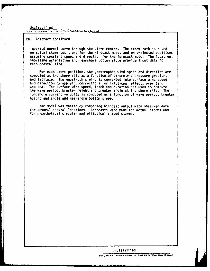
Unclassified.. lT' CLASSIFICATION OF THIS PAGE(Whof Dag Entered)

20. Abstract continued

inverted normal curve through the storm center. The storm path is basedon actual storm positions for the hindcast mode, and on projected positionsassuming constant speed and direction for the forecast mode. The location,shoreline orientation and nearshore bottom slope provide input data foreach coastal site.

For each storm position, the geostrophic wind speed and direction arecomputed at the shore site as a function of barometric pressure gradientand latitude. The geostrophic wind is converted into surface wind speedand direction by applying corrections for frictional effects over landand sea. The surface wind speed, fetch and duration are used to computethe wave period, breaker height and breaker angle at the shore site. Thelongshore current velocity is computed as a function of wave period, breakerheight and angle and nearshore bottom slope.

The model was tested by comparing hindcast output with observed datafor several coastal locations. Forecasts were made for actual storms andfor hypothetical circular and elliptical shaped storms.

Unclassifiled$6rUMITV CLASSIFICATION OF THIS PAGE"'n Dfle EnteRfod)