Flight Envelope Calculation of a Hypersonic Vehicle Using ...dalle/presentations/conferences/DalleISP... · 2D aerodynamic model ... Heating,” Aeronautical Engineering Review, Vol

Scramjet FlightEnvelope

Dalle et. al.

Motivation

Vehicle modelInlet

Combustor

Nozzle

Integration

Flight dynamicsTrim

Linearization

ResultsOperating maps

Linearized system

Future work

Conclusions

AppendixOperating maps

Validation

References

Flight Envelope Calculation of aHypersonic Vehicle Using a

First Principles-Derived Model17th AIAA International Space Planes and Hypersonic Systems and

Technologies Conference

Derek J. DalleUniversity of Michigan, Ann Arbor, MI 48109

Michael A. BolenderU.S. Air Force Research Laboratory, Ohio, 45433

Sean M. Torrez, James F. DriscollUniversity of Michigan, Ann Arbor, MI 48109

April 14, 2011

CCCS

Scramjet Flight Envelope, HYTASP 2011 1/39


Dalle et. al.

Motivation

Vehicle modelInlet

Combustor

Nozzle

Integration

Flight dynamicsTrim

Linearization


Linearized system

Future work

Conclusions


Validation

References

Motivation

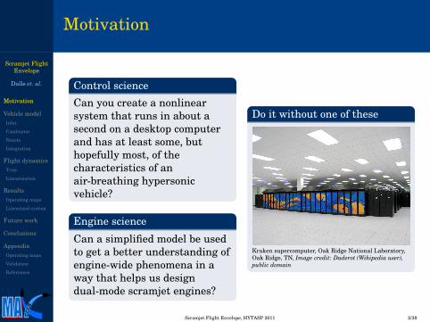
Control science

Can you create a nonlinearsystem that runs in about asecond on a desktop computerand has at least some, buthopefully most, of thecharacteristics of anair-breathing hypersonicvehicle?

Engine science

Can a simplified model be usedto get a better understanding ofengine-wide phenomena in away that helps us designdual-mode scramjet engines?

Do it without one of these

Kraken supercomputer, Oak Ridge National Laboratory,Oak Ridge, TN, Image credit: Daderot (Wikipedia user),public domain

CCCS



Dalle et. al.

Motivation

Vehicle modelInlet

Combustor

Nozzle

Integration

Flight dynamicsTrim

Linearization


Linearized system

Future work

Conclusions


Validation

References

Why dual-mode ram/scram again?

Competition

Space access: rocket

High-speed, long-range:rocket with glide

High-speed loiter: ?

Maximum practical Machnumber is about 12

We’ve all seen this one before.

Mach Number

Spe

cifi

c Im

puls

e [s

]

8,000

7,000

6,000

5,000

4,000

3,000

2,000

1,000

00 2 4 6 8 10

Turbofan

Turbofan with afterburner Ramjet

Scramjet

Rocket

Theoretical maximumHydrocarbon fuel in air

Theoretical maximumHydrogen fuel in air

For applications where we use lift, doubling the specific impulseis a big increase

Wide range of applications

Possibility of a large flight envelope

CCCS



Dalle et. al.

Motivation

Vehicle modelInlet

Combustor

Nozzle

Integration

Flight dynamicsTrim

Linearization


Linearized system

Future work

Conclusions


Validation

References

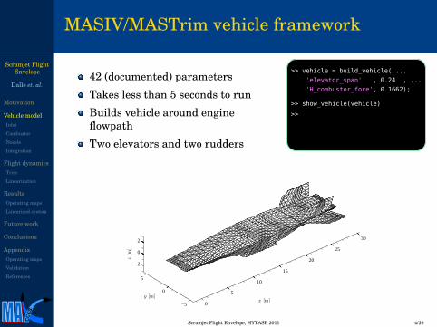
MASIV/MASTrim vehicle framework

42 (documented) parameters

Takes less than 5 seconds to run

Builds vehicle around engineflowpath

Two elevators and two rudders

>> vehicle = build_vehicle( ...

'elevator_span' , 0.24 , ...

'H_combustor_fore', 0.1662);

>> show_vehicle(vehicle)

>>

0

5

10

15

20

25

30

−5

0

5

−2

0

2

x [m]y [m]

z[m

]

CCCS



Dalle et. al.

Motivation

Vehicle modelInlet

Combustor

Nozzle

Integration

Flight dynamicsTrim

Linearization


Linearized system

Future work

Conclusions


Validation

References

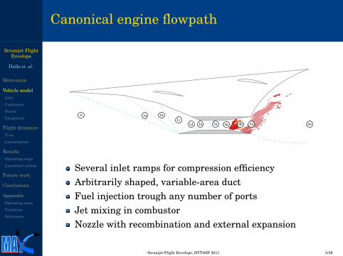
Canonical engine flowpath

8 1a 1b1c

1d 2a 3a 4a 4b 5a 6a

Several inlet ramps for compression efficiencyArbitrarily shaped, variable-area ductFuel injection trough any number of portsJet mixing in combustorNozzle with recombination and external expansion

CCCS



Dalle et. al.

Motivation

Vehicle modelInlet

Combustor

Nozzle

Integration

Flight dynamicsTrim

Linearization


Linearized system

Future work

Conclusions


Validation

References

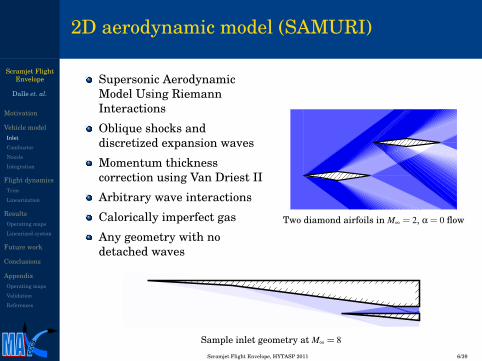
2D aerodynamic model (SAMURI)

Supersonic AerodynamicModel Using RiemannInteractions

Oblique shocks anddiscretized expansion waves

Momentum thicknesscorrection using Van Driest II

Arbitrary wave interactions

Calorically imperfect gas

Any geometry with nodetached waves

Two diamond airfoils in M∞ = 2, α = 0 flow

Sample inlet geometry at M∞ = 8

CCCS



Dalle et. al.

Motivation

Vehicle modelInlet

Combustor

Nozzle

Integration

Flight dynamicsTrim

Linearization


Linearized system

Future work

Conclusions


Validation

References

Riemann problem

Discontinuous regionscome in contact whenshocks intersectRegions B and C musthave the same pressureDensity and temperaturemay differFlow matches directionWaves separate regions Afrom B and D from CMain limiter of codeperformance

Zoom in on a generic flow

A

B

C

D

σA

βAθA

θB

θD

σC

σD

μC

μD

Sketch of two interacting waves.

CCCS



Dalle et. al.

Motivation

Vehicle modelInlet

Combustor

Nozzle

Integration

Flight dynamicsTrim

Linearization


Linearized system

Future work

Conclusions


Validation

References

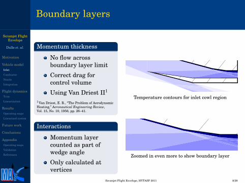
Boundary layers

Momentum thickness

No flow acrossboundary layer limit

Correct drag forcontrol volume

Using Van Driest II1

1Van Driest, E. R., “The Problem of AerodynamicHeating,” Aeronautical Engineering Review,Vol. 15, No. 10, 1956, pp. 26–41.

Interactions

Momentum layercounted as part ofwedge angle

Only calculated atvertices

Temperature contours for inlet cowl region

Zoomed in even more to show boundary layer

CCCS



Dalle et. al.

Motivation

Vehicle modelInlet

Combustor

Nozzle

Integration

Flight dynamicsTrim

Linearization


Linearized system

Future work

Conclusions


Validation

References

Comparison to CFD

Results from CFD++

Results from SAMURI

Darker colors represent higher pressures: maximum p/p∞ = 90

Maximum local error is about 6%Viscous CFD, no boundary layers in SAMURI

CCCS



Dalle et. al.

Motivation

Vehicle modelInlet

Combustor

Nozzle

Integration

Flight dynamicsTrim

Linearization


Linearized system

Future work

Conclusions


Validation

References

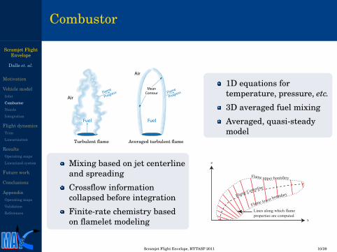
Combustor

Fuel

AirFlam

e

Progress

Fuel

Air

Flame

Progress

MeanContour

Turbulent flame Averaged turbulent flame

1D equations fortemperature, pressure, etc.

3D averaged fuel mixing

Averaged, quasi-steadymodel

Mixing based on jet centerlineand spreading

Crossflow informationcollapsed before integration

Finite-rate chemistry basedon flamelet modeling

Lines along which flameproperties are computed

z

x

Flame lower boundaryFlame Centerline

Flame upper boundary

CCCS



Dalle et. al.

Motivation

Vehicle modelInlet

Combustor

Nozzle

Integration

Flight dynamicsTrim

Linearization


Linearized system

Future work

Conclusions


Validation

References

Nozzle modelAlmost the same as the inlet

Results from CFD++

1200

700

200

400

400

Results from fundamental model

Pressure contours

This comparison included finite-rate chemistry

CFD model included viscosity

CCCS



Dalle et. al.

Motivation

Vehicle modelInlet

Combustor

Nozzle

Integration

Flight dynamicsTrim

Linearization


Linearized system

Future work

Conclusions


Validation

References

Forces on each panel

Include angular velocity of each panel

uk = ubes = ub

eb + ωbeb× rb

bs

Project velocity onto triangle and find deflection

uk = nk× uk sinδk =− nk ·uk

‖uk‖

Use Prandtl-Meyer theory if δk < 0 and shock if δk > 0

If 0 < δk ≤ δmax, use oblique shock relation

tanδk = 2cotβkM2

k sin2βk−1

M2k (γ + cos2βk) + 2

If shock is detached, interpolate the shock angle

β = βmax +δk−δmax

π/2−δmax(π/2−βmax)

Use momentum thickness from the upstream panels; use Van Driest II

Calculate momentum thickness on downstream edges

CCCS



Dalle et. al.

Motivation

Vehicle modelInlet

Combustor

Nozzle

Integration

Flight dynamicsTrim

Linearization


Linearized system

Future work

Conclusions


Validation

References

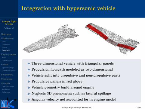
Integration with hypersonic vehicle

Three-dimensional vehicle with triangular panels

Propulsion flowpath modeled as two-dimensional

Vehicle split into propulsive and non-propulsive parts

Propulsive panels in red above

Vehicle geometry build around engine

Neglects 3D phenomena such as lateral spillage

Angular velocity not accounted for in engine model

CCCS



Dalle et. al.

Motivation

Vehicle modelInlet

Combustor

Nozzle

Integration

Flight dynamicsTrim

Linearization


Linearized system

Future work

Conclusions


Validation

References

Earth model

prime meridian

equatorxe

ye

ze

xn yn

zn

Equations of motion

Rotating, ellipsoidal Earthdefault (WGS84)

Options for flat or sphericalEarth

Rotation can be turned on oroff independently

Submodels

Somigliana gravity model

1976 standard atmosphere

Optional temperature offset

Optional wind and windderivatives

CCCS



Dalle et. al.

Motivation

Vehicle modelInlet

Combustor

Nozzle

Integration

Flight dynamicsTrim

Linearization


Linearized system

Future work

Conclusions


Validation

References

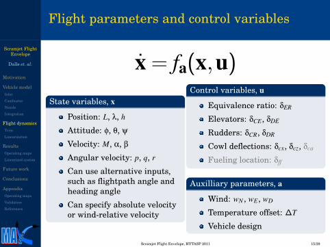
Flight parameters and control variables

x = fa(x,u)State variables, x

Position: L, λ, h

Attitude: φ, θ, ψ

Velocity: M, α, β

Angular velocity: p, q, r

Can use alternative inputs,such as flightpath angle andheading angle

Can specify absolute velocityor wind-relative velocity

Control variables, u

Equivalence ratio: δER

Elevators: δCE, δDE

Rudders: δCR, δDR

Cowl deflections: δcx, δcz, δca

Fueling location: δff

Auxilliary parameters, a

Wind: wN , wE, wD

Temperature offset: ∆T

Vehicle design

CCCS



Dalle et. al.

Motivation

Vehicle modelInlet

Combustor

Nozzle

Integration

Flight dynamicsTrim

Linearization


Linearized system

Future work

Conclusions


Validation

References

Vehicle trim

Problem statement:

Find x and u such thatx = f(x,u)

where we pick the value of x beforehand. Usually we want x = 0.

Independent variables and dependent variables

We want to pick some of the state variables beforehand, but not all.

ξ = T1x υ =

[T2xu

]Now ξ has independent variables, and υ has dependent variables.

Implementation

Technically that’s only an equality constraint.

min φ(ξ,υ) subject to υ = g(ξ, x)

CCCS



Dalle et. al.

Motivation

Vehicle modelInlet

Combustor

Nozzle

Integration

Flight dynamicsTrim

Linearization


Linearized system

Future work

Conclusions


Validation

References

Vehicle trim

Problem statement:





ξ = T1x υ =

[T2xu


Implementation



CCCS



Dalle et. al.

Motivation

Vehicle modelInlet

Combustor

Nozzle

Integration

Flight dynamicsTrim

Linearization


Linearized system

Future work

Conclusions


Validation

References

Vehicle trim

Problem statement:





ξ = T1x υ =

[T2xu


Implementation

Solving for υ gives us a trim function.

υ = g(ξ, x)

Implementation



CCCS



Dalle et. al.

Motivation

Vehicle modelInlet

Combustor

Nozzle

Integration

Flight dynamicsTrim

Linearization


Linearized system

Future work

Conclusions


Validation

References

Vehicle trim

Problem statement:





ξ = T1x υ =

[T2xu


Implementation



CCCS



Dalle et. al.

Motivation

Vehicle modelInlet

Combustor

Nozzle

Integration

Flight dynamicsTrim

Linearization


Linearized system

Future work

Conclusions


Validation

References

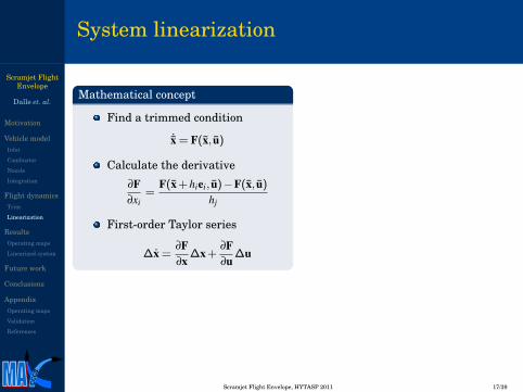
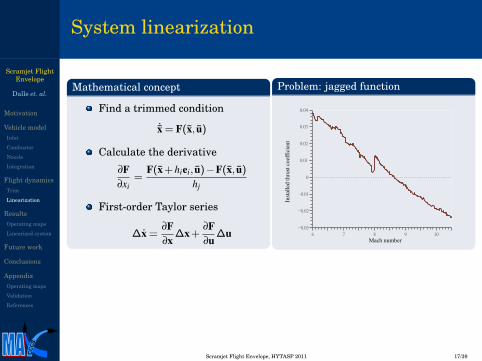
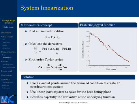
System linearization

Mathematical concept

Find a trimmed condition

˙x = F(x, u)

Calculate the derivative

∂F∂xi

=F(x + hiei, u)−F(x, u)

hj

First-order Taylor series

∆x =∂F∂x

∆x +∂F∂u

∆u

Problem: jagged function

6 7 8 9 10−0.03

−0.02

−0.01

0

0.01

0.02

0.03

0.04

Mach number

Inst

alle

d th

rust

coe

ffic

ient

Solution

Use a cloud of points around the trimmed condition to create anoverdetermined system

Use linear least squares to solve for the best-fitting plane

Result is hopefully the derivative of the underlying function

CCCS



Dalle et. al.

Motivation

Vehicle modelInlet

Combustor

Nozzle

Integration

Flight dynamicsTrim

Linearization


Linearized system

Future work

Conclusions


Validation

References




˙x = F(x, u)


∂F∂xi


hj


∆x =∂F∂x

∆x +∂F∂u

∆u


6 7 8 9 10−0.03

−0.02

−0.01

0

0.01

0.02

0.03

0.04

Mach number

Inst

alle

d th

rust

coe

ffic

ient

Solution




CCCS



Dalle et. al.

Motivation

Vehicle modelInlet

Combustor

Nozzle

Integration

Flight dynamicsTrim

Linearization


Linearized system

Future work

Conclusions


Validation

References




˙x = F(x, u)


∂F∂xi


hj


∆x =∂F∂x

∆x +∂F∂u

∆u


6 7 8 9 10−0.03

−0.02

−0.01

0

0.01

0.02

0.03

0.04

Mach number

Inst

alle

d th

rust

coe

ffic

ient

Solution




CCCS



Dalle et. al.

Motivation

Vehicle modelInlet

Combustor

Nozzle

Integration

Flight dynamicsTrim

Linearization


Linearized system

Future work

Conclusions


Validation

References

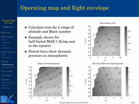
Operating map and flight envelope

Calculate trim for a range ofaltitude and Mach number

Example shown forhalf-fueled MAX-1 flying eastat the equator

Dotted lines show dynamicpressure in atmospheres

Equivalence ratio

0.4

0.4

0.6

0.6

0.6

0.8

0.8

0.8

1

1

1

1.2

1.2

1.4

1.4 1.6 1.8 2

M

h[km]

6 7 8 9 1024

25

26

27

28

29

30

31

32

0.3

0.4

0.5

0.6

Angle of attack [degrees]

0.4

0.4

0.6

0.6

0.6

0.8

0.8

0.8

1

1

1

1.2

1.2

1.4

1.4 1.6 1.8 2

M

h[km]

6 7 8 9 1024

25

26

27

28

29

30

31

32

0

0.5

1

1.5

2

Elevator deflection angle [degrees]

0.4

0.4

0.6

0.6

0.6

0.8

0.8

0.8

1

1

1

1.2

1.2

1.4

1.4 1.6 1.8 2

M

h[km]

6 7 8 9 1024

25

26

27

28

29

30

31

32

1

2

3

4

CCCS



Dalle et. al.

Motivation

Vehicle modelInlet

Combustor

Nozzle

Integration

Flight dynamicsTrim

Linearization


Linearized system

Future work

Conclusions


Validation

References

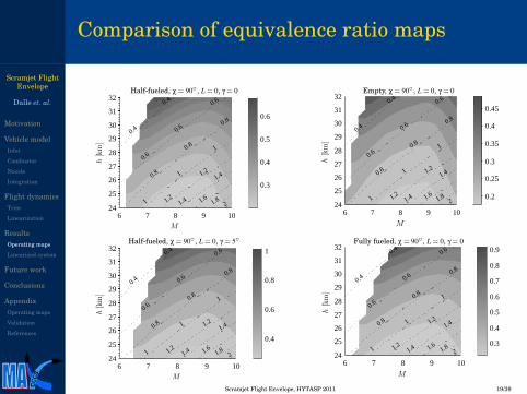
Comparison of equivalence ratio maps

Half-fueled, χ = 90◦ , L = 0, γ = 0

0.4

0.4

0.6

0.6

0.6

0.8

0.8

0.8

1

1

1

1.2

1.2

1.4

1.4 1.6 1.8 2

M

h[km]

6 7 8 9 1024

25

26

27

28

29

30

31

32

0.3

0.4

0.5

0.6

Half-fueled, χ = 90◦ , L = 0, γ = 5◦

0.4

0.4

0.6

0.6

0.6

0.8

0.8

0.8

1

1

1

1.2

1.2

1.4

1.4 1.6 1.8 2

M

h[km]

6 7 8 9 1024

25

26

27

28

29

30

31

32

0.4

0.6

0.8

1

Empty, χ = 90◦ , L = 0, γ = 0

0.4

0.4

0.6

0.6

0.6

0.8

0.8

0.8

1

1

1

1.2

1.2

1.4

1.4 1.6 1.8 2

M

h[km]

6 7 8 9 1024

25

26

27

28

29

30

31

32

0.2

0.25

0.3

0.35

0.4

0.45

Fully fueled, χ = 90◦ , L = 0, γ = 0

0.4

0.4

0.6

0.6

0.6

0.8

0.8

0.8

1

1

1

1.2

1.2

1.4

1.4 1.6 1.8 2

M

h[km]

6 7 8 9 1024

25

26

27

28

29

30

31

32

0.3

0.4

0.5

0.6

0.7

0.8

0.9

CCCS



Dalle et. al.

Motivation

Vehicle modelInlet

Combustor

Nozzle

Integration

Flight dynamicsTrim

Linearization


Linearized system

Future work

Conclusions


Validation

References

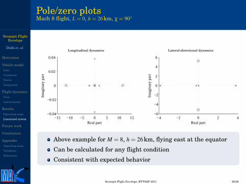
Pole/zero plotsMach 8 flight, L = 0, h = 26km, χ = 90◦

Longitudinal dynamics

−15 −10 −5 0 5 10 15−0.04

−0.02

0

0.02

0.04

Real part

Imag

inar

y pa

rt

Lateral-directional dynamics

−4 −2 0 2 4−6

−4

−2

0

2

4

6

Real part

Imag

inar

y pa

rt

Above example for M = 8, h = 26km, flying east at the equator

Can be calculated for any flight condition

Consistent with expected behavior

CCCS



Dalle et. al.

Motivation

Vehicle modelInlet

Combustor

Nozzle

Integration

Flight dynamicsTrim

Linearization


Linearized system

Future work

Conclusions


Validation

References

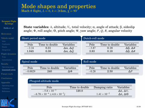
Mode shapes and propertiesMach 8 flight, L = 0, h = 26km, χ = 90◦

State variables: h, altitude; Vt, total velocity; α, angle of attack; β, sideslipangle; Φ, roll angle; Θ, pitch angle; Ψ, yaw angle; P, Q, R, angular velocity

Short period mode

Pole Time to double Variables−2.24 0.31 ∆α, ∆Q1.845 0.38 ∆α, ∆Q

Spiral mode

Pole Time to double Variables−0.0029 240 ∆Φ

Dutch-roll mode

Pole Time to double Variables−3.87 0.18 ∆β, ∆R3.83 0.18 ∆β, ∆R

Roll mode

Pole Time to double Variables−0.28 2.50 ∆P

Phugoid-altitude mode

Pole Time to double Damping ratio Variables−5.8×10−3 120.0 ∆h, ∆Vt

−6.78×10−4±4.8×10−2j 1.41×10−2 ∆h, ∆Θ

CCCS



Dalle et. al.

Motivation

Vehicle modelInlet

Combustor

Nozzle

Integration

Flight dynamicsTrim

Linearization


Linearized system

Future work

Conclusions


Validation

References

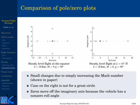
Comparison of pole/zero plots

−15 −10 −5 0 5 10 15−6

−4

−2

0

2

4

6

Real part

Imag

inar

y pa

rt

Steady, level flight at the equatorh = 26 km, M = 8 χ = 90◦

−5 0 5 10 15 20

−5

0

5

Real part

Imag

inar

y pa

rt

Steady, level flight at L = 45◦Nh = 26 km, M = 8, χ = 90◦

Small changes due to simply increasing the Mach number(shown in paper)

Case on the right is not for a great circle

Zeros move off the imaginary axis because the vehicle has anonzero roll angle

CCCS



Dalle et. al.

Motivation

Vehicle modelInlet

Combustor

Nozzle

Integration

Flight dynamicsTrim

Linearization


Linearized system

Future work

Conclusions


Validation

References

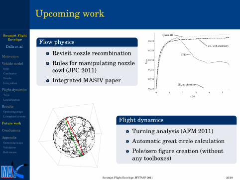
Upcoming work

Flow physics

Revisit nozzle recombination

Rules for manipulating nozzlecowl (JPC 2011)

Integrated MASIV paper

0 1 2 3 4 50.228

0.230

0.232

0.234

0.236

0.238

x [m]

Y H2O

Quasi-1D

CFD

2D, no chemistry

2D, with chemistry

Flight dynamics

Turning analysis (AFM 2011)

Automatic great circle calculation

Pole/zero figure creation (withoutany toolboxes)

CCCS



Dalle et. al.

Motivation

Vehicle modelInlet

Combustor

Nozzle

Integration

Flight dynamicsTrim

Linearization


Linearized system

Future work

Conclusions


Validation

References

Conclusions

Flight envelope

Approximately 1400 trimmedflight conditions

Initial estimation of operatingmap for altitude and Machnumber

Dynamics

Linearization about threeflight conditions

Stability and modal analysis

Rotating, ellipsoidal Earth

Does it mean anything?

Limited to medium fidelity for a limited class of vehicles

No proper upper bound on Mach number

Modeling physics directly gives some amount of predictive ability

Demonstrated ability to predict some non-obvious performance

CCCS



Dalle et. al.

Motivation

Vehicle modelInlet

Combustor

Nozzle

Integration

Flight dynamicsTrim

Linearization


Linearized system

Future work

Conclusions


Validation

References

Acknowledgments

This research was supported by U.S. Air Force ResearchLaboratory grant FA 8650-07-2-3744 for the Michigan AirForce Research Laboratory Collaborative Center forControl Science.Approved for Public Release; Distribution Unlimited. CaseNumber 88ABW-2011-1250Nicolas LamorteScott G. V. FrendreisThis research was completed as part of theMichigan/AFRL Collaborative Center for Control Science

CCCS



Dalle et. al.

Motivation

Vehicle modelInlet

Combustor

Nozzle

Integration

Flight dynamicsTrim

Linearization


Linearized system

Future work

Conclusions


Validation

References

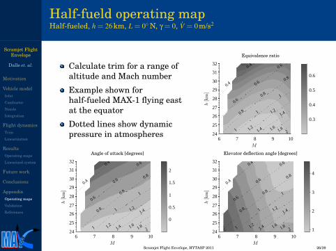
Half-fueld operating mapHalf-fueled, h = 26km, L = 0◦N, γ = 0, V = 0m/s2


Example shown forhalf-fueled MAX-1 flying eastat the equator


Equivalence ratio

0.4

0.4

0.6

0.6

0.6

0.8

0.8

0.8

1

1

1

1.2

1.2

1.4

1.4 1.6 1.8 2

M

h[km]

6 7 8 9 1024

25

26

27

28

29

30

31

32

0.3

0.4

0.5

0.6


0.4

0.4

0.6

0.6

0.6

0.8

0.8

0.8

1

1

1

1.2

1.2

1.4

1.4 1.6 1.8 2

M

h[km]

6 7 8 9 1024

25

26

27

28

29

30

31

32

0

0.5

1

1.5

2


0.4

0.4

0.6

0.6

0.6

0.8

0.8

0.8

1

1

1

1.2

1.2

1.4

1.4 1.6 1.8 2

M

h[km]

6 7 8 9 1024

25

26

27

28

29

30

31

32

1

2

3

4

CCCS



Dalle et. al.

Motivation

Vehicle modelInlet

Combustor

Nozzle

Integration

Flight dynamicsTrim

Linearization


Linearized system

Future work

Conclusions


Validation

References

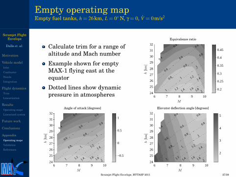
Empty operating mapEmpty fuel tanks, h = 26km, L = 0◦N, γ = 0, V = 0m/s2


Example shown for emptyMAX-1 flying east at theequator


Equivalence ratio

0.4

0.4

0.6

0.6

0.6

0.8

0.8

0.8

1

1

1

1.2

1.2

1.4

1.4 1.6 1.8 2

M

h[km]

6 7 8 9 1024

25

26

27

28

29

30

31

32

0.2

0.25

0.3

0.35

0.4

0.45


0.4

0.4

0.6

0.6

0.6

0.8

0.8

0.8

1

1

1

1.2

1.2

1.4

1.4 1.61.8

2

M

h[km]

6 7 8 9 1024

25

26

27

28

29

30

31

32

−0.5

0

0.5

1


0.4

0.4

0.6

0.6

0.6

0.8

0.8

0.8

1

1

1

1.2

1.2

1.4

1.4 1.6 1.8 2

M

h[km]

6 7 8 9 1024

25

26

27

28

29

30

31

32

2

3

4

5

CCCS



Dalle et. al.

Motivation

Vehicle modelInlet

Combustor

Nozzle

Integration

Flight dynamicsTrim

Linearization


Linearized system

Future work

Conclusions


Validation

References

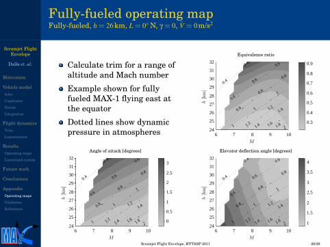
Fully-fueled operating mapFully-fueled, h = 26km, L = 0◦N, γ = 0, V = 0m/s2


Example shown for fullyfueled MAX-1 flying east atthe equator


Equivalence ratio

0.4

0.4

0.6

0.6

0.6

0.8

0.8

0.8

1

1

1

1.2

1.2

1.4

1.4 1.6 1.8 2

M

h[km]

6 7 8 9 1024

25

26

27

28

29

30

31

32

0.3

0.4

0.5

0.6

0.7

0.8

0.9


0.4

0.4

0.6

0.6

0.6

0.8

0.8

0.8

1

1

1

1.2

1.2

1.4

1.4 1.6 1.8 2

M

h[km]

6 7 8 9 1024

25

26

27

28

29

30

31

32

0

0.5

1

1.5

2

2.5

3


0.4

0.4

0.6

0.6

0.6

0.8

0.8

0.8

1

1

1

1.2

1.2

1.4

1.4 1.6 1.8 2

M

h[km]

6 7 8 9 1024

25

26

27

28

29

30

31

32

1

1.5

2

2.5

3

3.5

4

CCCS



Dalle et. al.

Motivation

Vehicle modelInlet

Combustor

Nozzle

Integration

Flight dynamicsTrim

Linearization


Linearized system

Future work

Conclusions


Validation

References

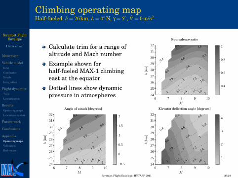
Climbing operating mapHalf-fueled, h = 26km, L = 0◦N, γ = 5◦, V = 0m/s2


Example shown forhalf-fueled MAX-1 climbingeast at the equator


Equivalence ratio

0.4

0.4

0.6

0.6

0.6

0.8

0.8

0.8

1

1

1

1.2

1.2

1.4

1.4 1.6 1.8 2

M

h[km]

6 7 8 9 1024

25

26

27

28

29

30

31

32

0.4

0.6

0.8

1


0.4

0.4

0.6

0.6

0.6

0.8

0.8

0.8

1

1

1

1.2

1.2

1.4

1.4 1.61.8

2

M

h[km]

6 7 8 9 1024

25

26

27

28

29

30

31

32

−0.5

0

0.5

1

1.5

2


0.4

0.4

0.6

0.6

0.6

0.8

0.8

0.8

1

1

1

1.2

1.2

1.4

1.4 1.6 1.8 2

M

h[km]

6 7 8 9 1024

25

26

27

28

29

30

31

32

1

2

3

4

CCCS



Dalle et. al.

Motivation

Vehicle modelInlet

Combustor

Nozzle

Integration

Flight dynamicsTrim

Linearization


Linearized system

Future work

Conclusions


Validation

References

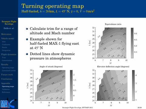
Turning operating mapHalf-fueled, h = 26km, L = 45◦N, γ = 0, V = 0m/s2


Example shown forhalf-fueled MAX-1 flying eastat 45◦N


Equivalence ratio

0.4

0.4

0.6

0.6

0.6

0.8

0.8

0.8

1

1

1

1.2

1.2

1.4

1.4 1.6 1.8 2

M

h[km]

6 7 8 9 1024

25

26

27

28

29

30

31

32

0.3

0.4

0.5

0.6


0.4

0.4

0.6

0.6

0.6

0.8

0.8

0.8

1

1

1

1.2

1.2

1.4

1.4 1.6 1.8 2

M

h[km]

6 7 8 9 1024

25

26

27

28

29

30

31

32

0

0.5

1

1.5

2


0.4

0.4

0.6

0.6

0.6

0.8

0.8

0.8

1

1

1

1.2

1.2

1.4

1.4 1.6 1.8 2

M

h[km]

6 7 8 9 1024

25

26

27

28

29

30

31

32

1

2

3

4

CCCS



Dalle et. al.

Motivation

Vehicle modelInlet

Combustor

Nozzle

Integration

Flight dynamicsTrim

Linearization


Linearized system

Future work

Conclusions


Validation

References

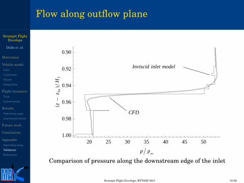
Flow along outflow plane

Inviscid inlet model

CFD

20 25 30 35 40 45 501.00

0.98

0.96

0.94

0.92

0.90

p � p¥

Hz -

z1a

L� H

1

Comparison of pressure along the downstream edge of the inlet

CCCS



Dalle et. al.

Motivation

Vehicle modelInlet

Combustor

Nozzle

Integration

Flight dynamicsTrim

Linearization


Linearized system

Future work

Conclusions


Validation

References

Experiment of Emami et. al.

Experimental apparatus schematica

aEmami, S., Trexler, C. A., Auslender, A. H., and Weidner, J. P., “Experimental Investigation of Inlet-Combustor Isolatorsfor a Dual-Mode Scramjet at a Mach Number of 4,” NASA Technical Paper 3502, May 1995

Inlet experiment, M∞ = 4.0

Movable cowl anglePressure taps along surfaceRelatively narrow inlet

CCCS



Dalle et. al.

Motivation

Vehicle modelInlet

Combustor

Nozzle

Integration

Flight dynamicsTrim

Linearization


Linearized system

Future work

Conclusions


Validation

References

Experiment of Emami et. al.

SAMURI solution for the Emami et. al.geometry with θcl = 6.5◦

DescriptionPrimary ramp angle is 11◦

Cowl angle range: 0◦ to 11◦

Three cowl lengthsAlso controls area ratioLength/width ratio 5.0

Coordinates

Surface LengthInlet ramp (horizontal) 24.816cmInlet ramp (vertical) 4.8260cmIsolator height 1.0160cmForward cowl length 11.176cmIsolator width 5.0800cm

CCCS



Dalle et. al.

Motivation

Vehicle modelInlet

Combustor

Nozzle

Integration

Flight dynamicsTrim

Linearization


Linearized system

Future work

Conclusions


Validation

References

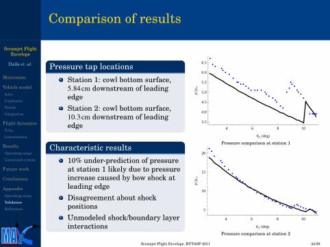
Comparison of results

Pressure tap locationsStation 1: cowl bottom surface,5.84cm downstream of leadingedgeStation 2: cowl bottom surface,10.3cm downstream of leadingedge

Characteristic results10% under-prediction of pressureat station 1 likely due to pressureincrease caused by bow shock atleading edgeDisagreement about shockpositionsUnmodeled shock/boundary layerinteractions

4 6 8 10

3.5

4.0

4.5

5.0

5.5

6.0

6.5

Θcl HdegL

p�p

¥

Pressure comparison at station 1

4 6 8 10

5

10

15

20

Θcl HdegL

p�p

¥

Pressure comparison at station 2

CCCS



Dalle et. al.

Motivation

Vehicle modelInlet

Combustor

Nozzle

Integration

Flight dynamicsTrim

Linearization


Linearized system

Future work

Conclusions


Validation

References

ReferencesWorks by other authors (1/2)

1 Anon., “Department of Defense World Geodetic System 1984,” Tech. Rep.TR 8350.2, 3rd ed., National Imagery and Mapping Agency (now NGA),1997.

2 Broyden, C. G., “A Class of Methods for Solving Nonlinear SimultaneousEquations,” Mathematics of Computation, Vol. 19, No. 92, October 1965,pp. 577-593

3 Chavez, F. R. and Schmidt, D. K., “Analytical Aeropropulsive/AeroelasticHypersonic-Vehicle Model with Dynamic Analysis,” Journal of Guidance,Control, and Dynamics, Vol. 17, No. 6, 1994, pp. 1308–1319.

4 Chudoba, B. “Aircraft Volume and Mass Guidelines,” National Instituteof Aerospace, June 2008, Hypersonic Educational Initiative HypersonicVehicle System Integration Short Course.

5 Durham, B., “Aircraft Dynamics & Control,”<http://www.aoe.vt.edu/durhamAOE5214>, accessed March 3, 2011.

6 Frendreis, S. G. V. and Cesnik, C. E. S., “3D Simulation of a FlexibleHypersonic Vehicle,” Atmospheric Flight Mechanics Conference &Exhibit, 2010, AIAA Paper 2010-8229.

CCCS



Dalle et. al.

Motivation

Vehicle modelInlet

Combustor

Nozzle

Integration

Flight dynamicsTrim

Linearization


Linearized system

Future work

Conclusions


Validation

References

ReferencesWorks by other authors (2/2)

7 Groves, P. D., Principles of GNSS, Inertial, and Multisensor IntegratedNavigations Systems, Artec House, 2008.

8 Hall, K. C., Thomas, J. P., and Dowell, E. H., “Proper OrthogonalDecomposition Technique for Transonic Unsteady Aerodynamic Flows,”AIAA Journal, Vol. 38, No. 10, 2000, pp. 1853–1862.

9 Savitzky, A. and Golay, M. J. E., “Smoothing and Differentiation of Databy Simplified Least Squares Procedures,” Analytical Chemistry, Vol. 36,No. 8, 1964, pp. 1627–1639.

10 Schöttle, U. M. and Hillesheimer, M., “Performance Optimization of anAirbreathing Launch Vehicle by a Sequential Trajectory Optimizationand Vehicle Design Scheme,” AIAA Guidance, Navigation, and ControlConference, 1991, AIAA Paper 91-2655.

11 Van Driest, E. R., “The Problem of Aerodynamic Heating,” AeronauticalEngineering Review, Vol. 15, No. 10, 1956, pp. 26–41.

12 White, F. M., Viscous Fluid Flow, McGraw-Hill, 3rd ed., 2006.13 Whittaker, S. E. and Robinson, G., The Calculus of Observations, Blackie

& Son, Limited, 1924.

CCCS



Dalle et. al.

Motivation

Vehicle modelInlet

Combustor

Nozzle

Integration

Flight dynamicsTrim

Linearization


Linearized system

Future work

Conclusions


Validation

References

ReferencesWorks by the authors (1/3)

1 Bolender, M. A. and Doman, D. B., “Nonlinear Longitudinal DynamicalModel of an Air-Breathing Hypersonic Vehicle,” Journal of Spacecraftand Rockets, Vol. 44, No. 2, 2007, pp. 274–387.

2 Dalle, D. J., Fotia, M. L., and Driscoll, J. F., “Reduced-Order Modeling ofTwo-Dimensional Supersonic Flows with Applications to ScramjetInlets,” Journal of Propulsion and Power, Vol. 26, No. 3, 2010,pp. 545–555.

3 Dalle, D. J., Frendreis, S. G. V., Driscoll, J. F., and Cesnik, C. E. S.,“Hypersonic Vehicle Flight Dynamics with Copuled Aerodynamics andReduced-order Propulsive Models,” AIAA Atmospheric Flight MechanicsConference & Exhibit, 2010, AIAA Paper 2010-7930.

CCCS



Dalle et. al.

Motivation

Vehicle modelInlet

Combustor

Nozzle

Integration

Flight dynamicsTrim

Linearization


Linearized system

Future work

Conclusions


Validation

References


4 Parker, J. T., Serrani, A., Yurkovich, S., Bolender, M. A., and Doman, D.B., “Control-Oriented Modeling of an Air-Breathing Hypersonic Vehicle,”Journal of Guidance, Control, and Dynamics, Vol. 30, No. 3, 2007, pp.856–869.

5 Torrez, S. M., Driscoll, J. F., Dalle, D. J., Bolender, M. A., and Doman, D.B., “Hypersonic Vehicle Thrust Sensitivity to Angle of Attack and MachNumber,” AIAA Atmospheric Flight Mechanics Conference & Exhibit,2010, AIAA Paper 2010-7930.

6 Torrez, S. M., Driscoll, J. F., Dalle, D. J., and Fotia, M. L., “PreliminaryDesign Methodology for Hypersonic Engine Flowpaths,” 16thAIAA/DLR/DGLR International Space Plances and Hypersonic Systemsand Technologies Conference, 2009, AIAA Paper 2009-7289.

CCCS



Dalle et. al.

Motivation

Vehicle modelInlet

Combustor

Nozzle

Integration

Flight dynamicsTrim

Linearization


Linearized system

Future work

Conclusions


Validation

References


7 Torrez, S. M., Driscoll, J. F., Ihme, M., and Fotia, M. L., “Reduced-OrderModeling of Turbulent Reacting Flows with Aplication to Scramjets,”Journal of Propulsion and Power, 2011.

8 Dalle, D. J., Torrez, S. M., and Driscoll, J. F., “Reduced-Order Modeling ofReacting Supersonic Flows in Scramjet Nozzles,” 46thAIAA/ASME/SAE/ASEE Joint Propulsion Conference and Exhibit,2010.

9 Torrez, S. M., Dalle, D. J., and Driscoll, J. F. “Dual Mode Scramjet Designto Achieve Improved Operational Stability,” 46thAIAA/ASME/SAE/ASEE Joint Propulsion Conference and Exhibit,2010.

10 Torrez, S. M., Driscoll, J. F., Dalle, D. J., and Micka, D. J. “ScramjetEngine Model MASIV: Role of Mixing, Chemistry, and Wave Interaction.”45th AIAA/ASME/SAE/ASEE Joint Propulsion Conference and Exhibit,2009.

CCCS


Documents

Flight Envelope Calculation of a Hypersonic Vehicle Using ...dalle/presentations/conferences/DalleISP... · 2D aerodynamic model ... Heating,” Aeronautical Engineering Review, Vol