Embed Size (px)
Citation preview
Flocking for Multi-Agent DynamicalSystems
by
Zhaoxin Wan
A thesispresented to the University of Waterloo
in fulfillment of thethesis requirement for the degree of
Master of Mathematicsin
Applied Mathematics
Waterloo, Ontario, Canada, 2012
c© Zhaoxin Wan 2012

I hereby declare that I am the sole author of this thesis. This is a true copy of the thesis,including any required final revisions, as accepted by my examiners.
I understand that my thesis may be made electronically available to the public.
ii
Abstract
In this thesis, we discuss models for multi-agent dynamical systems. We study thetracking/migration problem for flocks and a theoretical framework for design and analysisof flocking algorithm is presented. The interactions between agents in the systems aredenoted by potential functions that act as distance functions, hence, the design of properpotential functions are crucial in modelling and analyzing the flocking problem for multi-agent dynamical systems. Constructions for both non-smooth potential functions andsmooth potential functions with finite cut-off are investigated in detail.
The main contributions of this thesis are to extend the literature of continuous flockingmodels with impulsive control and delay. Lyapunov function techniques and techniques forstability of continuous and impulsive switching system are used, we study the asymptoticstability of the equilibrium of our models with impulsive control and discovery that byapplying impulsive control to Olfati-Saber’s continuous model, we can remove the dampingterm and improve the performance by avoiding the deficiency caused by time delay invelocity sensing.
Additionally, we discuss both free-flocking and constrained-flocking algorithm for multi-agent dynamical system, we extend literature results by applying velocity feedbacks whichare given by the dynamical obstacles in the environment to our impulsive control andsuccessfully lead to flocking with obstacle avoidance capability in a more energy-efficientway.
Simulations are given to support our results, some conclusions are made and futuredirections are given.
iii
Acknowledgements
First and foremost, I would like to thank my supervisor Xinzhi Liu and Wei-Chao Xie,whose guidance has been invaluable in my time as a graduate student. I would like to extenda great thanks to my examining committee, Matthew Scott and Sue Ann Campbell, bothof whom gave very helpful feedback, in the form of both corrections and suggestions. Iwould like to extend a thank you to the members of my research group: Mohamad Alwan,Jun Liu, Kexue Zhang, Hongtao Zhang, Shukai Li, Peter Stechlinski and Taghreed Subich,each of whom helped me either directly or indirectly with my research.
iv

Dedication
To my dear Parents and Brothers.
v
Table of Contents
List of Figures viii
1 Introduction 1
2 Muti-Agent Dynamical System Modelling 7
2.1 Basics of Graph Theory . . . . . . . . . . . . . . . . . . . . . . . . . . . . 8
2.1.1 Adjacency Matrix . . . . . . . . . . . . . . . . . . . . . . . . . . . . 10
2.1.2 Graph Laplacian . . . . . . . . . . . . . . . . . . . . . . . . . . . . 10
2.1.3 Particle-Based System . . . . . . . . . . . . . . . . . . . . . . . . . 12
2.2 Vicsek’s Discrete Model . . . . . . . . . . . . . . . . . . . . . . . . . . . . 14
2.3 Double Integrator Agents . . . . . . . . . . . . . . . . . . . . . . . . . . . . 15
2.3.1 Equation of Motion . . . . . . . . . . . . . . . . . . . . . . . . . . . 17
2.3.2 Potential Function Design . . . . . . . . . . . . . . . . . . . . . . . 17
3 Flocking via Continuous Control 25
3.1 α-Lattices and Quasi α-Lattices . . . . . . . . . . . . . . . . . . . . . . . . 26
3.2 Flocking Without Navigational Feedback . . . . . . . . . . . . . . . . . . . 27
3.2.1 Stable Flocking With Fixed Topology . . . . . . . . . . . . . . . . . 28
3.2.2 Stable Flocking With Switching Topologies . . . . . . . . . . . . . . 30
3.3 Flocking With Navigational Feeback . . . . . . . . . . . . . . . . . . . . . 31
3.3.1 Collective Dynamics . . . . . . . . . . . . . . . . . . . . . . . . . . 33
vi
3.3.2 Decomposition Dynamics . . . . . . . . . . . . . . . . . . . . . . . . 34
3.3.3 Stability Analysis . . . . . . . . . . . . . . . . . . . . . . . . . . . . 35
3.3.4 Simulation . . . . . . . . . . . . . . . . . . . . . . . . . . . . . . . . 40
3.4 Communication Time Delay . . . . . . . . . . . . . . . . . . . . . . . . . . 42
3.4.1 Without Navigational Feedback . . . . . . . . . . . . . . . . . . . . 43
3.4.2 With Navigational Feedback . . . . . . . . . . . . . . . . . . . . . . 46
3.5 Obstacle Avoidance Ability . . . . . . . . . . . . . . . . . . . . . . . . . . 49
3.5.1 Simulation . . . . . . . . . . . . . . . . . . . . . . . . . . . . . . . . 56
4 Flocking via Impulsive Control 58
4.1 Impulsive Consensus Problem . . . . . . . . . . . . . . . . . . . . . . . . . 58
4.2 Impulsive Flocking Problem . . . . . . . . . . . . . . . . . . . . . . . . . . 63
4.2.1 Without Damping . . . . . . . . . . . . . . . . . . . . . . . . . . . 64
4.2.2 Simulation . . . . . . . . . . . . . . . . . . . . . . . . . . . . . . . . 70
4.3 Coupling Time Delay . . . . . . . . . . . . . . . . . . . . . . . . . . . . . . 72
4.3.1 Simulation . . . . . . . . . . . . . . . . . . . . . . . . . . . . . . . . 76
4.4 Dynamic Obstacle Avoidance . . . . . . . . . . . . . . . . . . . . . . . . . 78
5 Conclusion and Future Direction 82
APPENDICES 85
A Convergent Analysis for Vicsek’s Model 86
References 92
vii
List of Figures
2.1 (a) A simple graph. (b) A graph with a loop . . . . . . . . . . . . . . . . 8
2.2 Graph (b) is a subgraph of graph (a) . . . . . . . . . . . . . . . . . . . . . 9
2.3 An agent and its neighbours in a spherical neighbourhood . . . . . . . . . 13
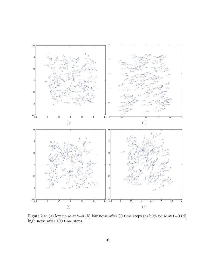
2.4 (a) low noise at t=0 (b) low noise after 30 time steps (c) high noise at t=0(d) high noise after 100 time steps . . . . . . . . . . . . . . . . . . . . . . 16
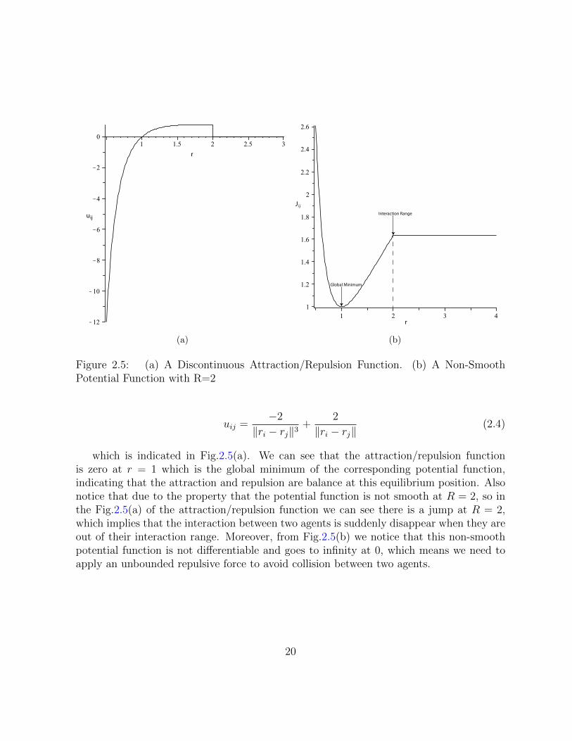
2.5 (a) A Discontinuous Attraction/Repulsion Function. (b) A Non-SmoothPotential Function with R=2 . . . . . . . . . . . . . . . . . . . . . . . . . 20
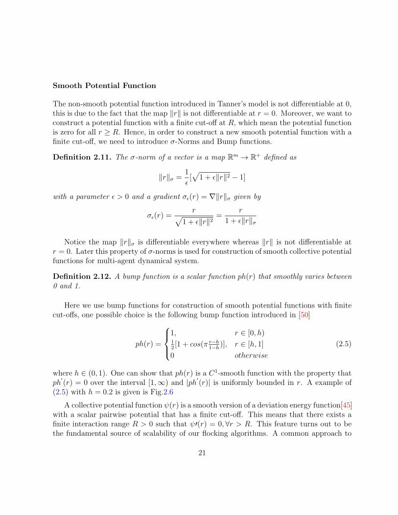
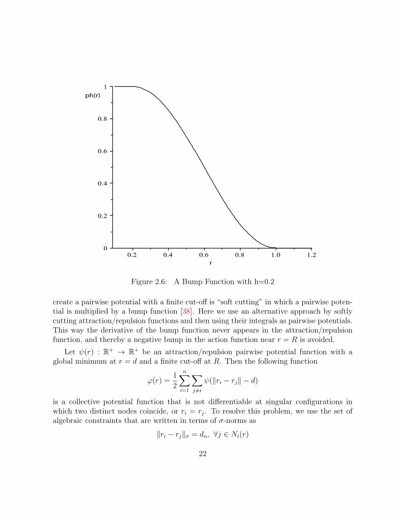
2.6 A Bump Function with h=0.2 . . . . . . . . . . . . . . . . . . . . . . . . . 22
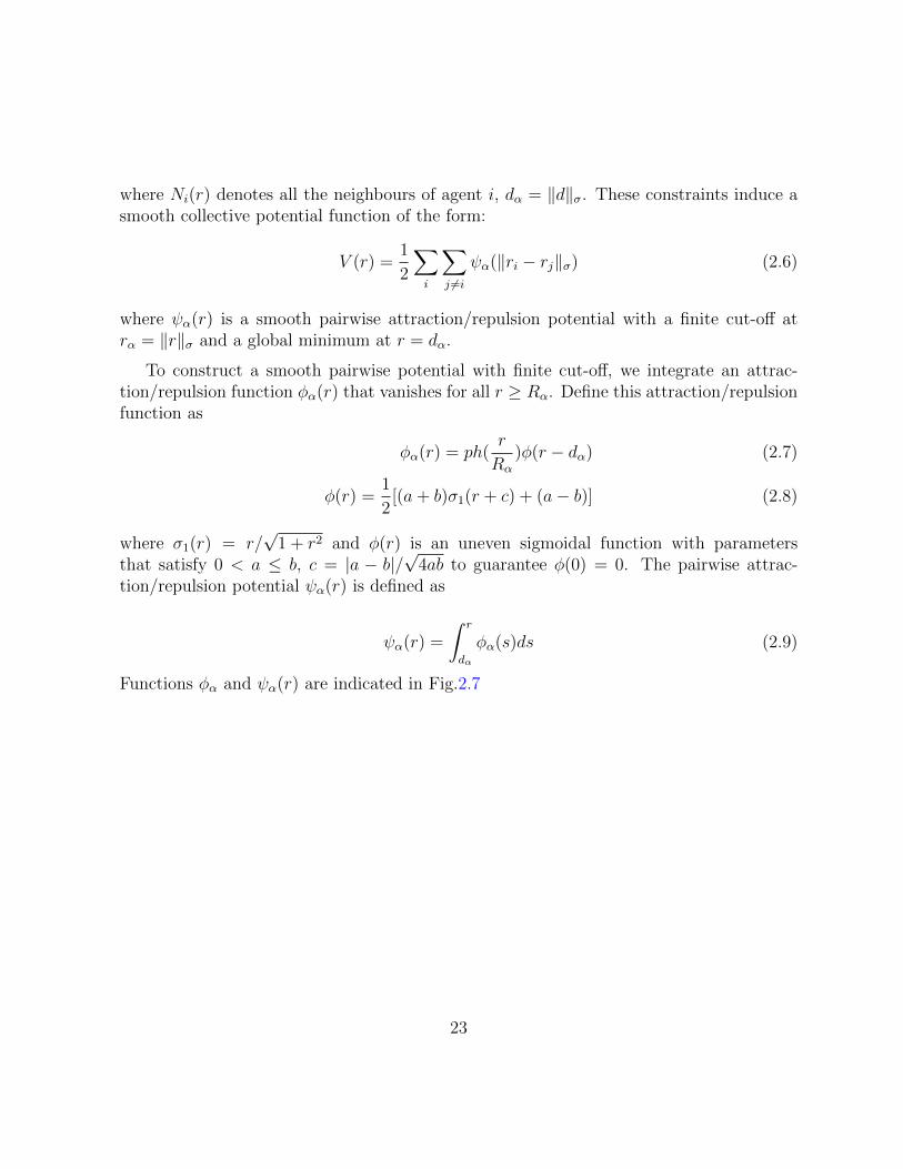
2.7 The Attraction/Repulsion an Potential Function with finite cut-offs : (a)φα(r), (b) ψα(r) . . . . . . . . . . . . . . . . . . . . . . . . . . . . . . . . . 24
3.1 Example of 2D α-lattices . . . . . . . . . . . . . . . . . . . . . . . . . . . . 26
3.2 Fragmentation Phenomenon . . . . . . . . . . . . . . . . . . . . . . . . . . 31
3.3 Flocking in Free-Space for n=50 agents. . . . . . . . . . . . . . . . . . . . 41
3.4 Velocity Mismatch . . . . . . . . . . . . . . . . . . . . . . . . . . . . . . . 42
3.5 β-agent representation of obstacles: (a) a wall and (b) a spherical obstacle. 50
3.6 A Repulsive Action Function with dβ = 6 . . . . . . . . . . . . . . . . . . . 52
3.7 Flocking in Presence of Obstacles for n=15 Agents and A Spherical Obstacle. 57
4.1 Flocking via Impulsive Control without Damping for n=50 agents. . . . . 71
4.2 Velocity Mismatch . . . . . . . . . . . . . . . . . . . . . . . . . . . . . . . 72
4.3 Flocking via Impulsive Control with Time Delay for n=50 agents. . . . . . 77
viii
4.4 Velocity Mismatch . . . . . . . . . . . . . . . . . . . . . . . . . . . . . . . 78
4.5 Flocking with dynamic obstacle avoidance . . . . . . . . . . . . . . . . . . 81
ix
Chapter 1
Introduction
The beautiful collective behaviour of swarming species such as some bacteria, ant colonies,bee colonies, flocks of birds, schools of fish and other have attracted and fascinated theinterest of researchers [19, 42, 41, 40, 37, 47, 59, 56, 52, 35, 27, 57, 39, 45] for manyyears. Collaborative flocking behaviour that we observe in these groups provides severaladvantages. The behaviour results in what is sometimes called “collective intelligence” or“swarm intelligence”, where groups of relatively simple and “unintelligent” individuals canaccomplish very complex tasks using only limited local information and simple rules ofbehaviour [23]. With the development of technology, including the technology on sensing,computation, information processing, power storage and others, it has become feasible todevelop engineered autonomous multi-agent dynamical systems such as systems composedof multi robots, satellites, or ground, air, surface, underwater or deep space vehicles.
The terminology of “swarms” has come to mean a set of agents possessing independentindividual dynamics but exhibiting intimately coupled behaviours and collectively perform-ing some tasks [23]. Another terminology to describe such system is the term “multi-agentdynamical systems”. Multi-agent dynamical systems have many potential commercial ap-plications such as pollution clear up, search and rescue operations, fire-fighter assistance,surveillance, demining operations and others. These applications range in many differentareas such as agriculture (for cultivation or applying pesticides for protection), forestry (forsurveillance and early detection of forest fires), in disaster areas (such as for search in ar-eas with radioactive release after a nuclear disaster), border patrol and homeland security,search and coverage in warehouses under fires, fire distinction, health care, etc [45].
In multi-agent dynamical systems, flocking is a form of collective behaviour of a largenumber of interacting agents with a common group objective [45]. In biology it is reserved
1
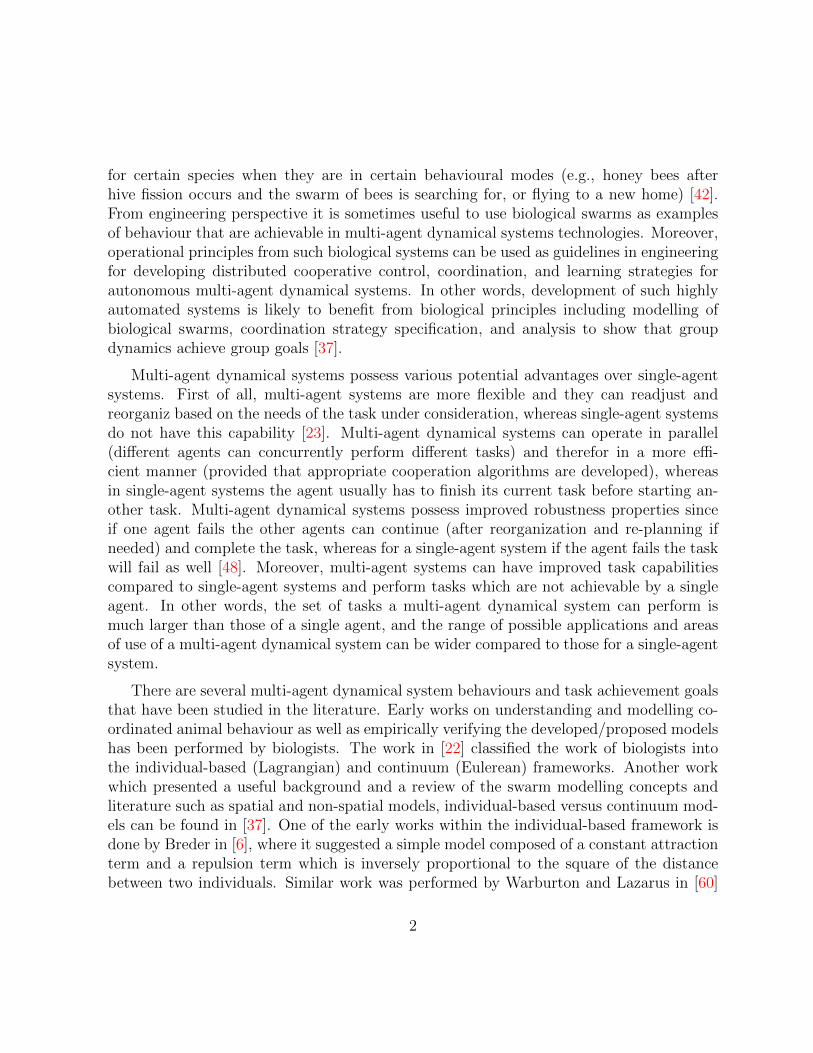
for certain species when they are in certain behavioural modes (e.g., honey bees afterhive fission occurs and the swarm of bees is searching for, or flying to a new home) [42].From engineering perspective it is sometimes useful to use biological swarms as examplesof behaviour that are achievable in multi-agent dynamical systems technologies. Moreover,operational principles from such biological systems can be used as guidelines in engineeringfor developing distributed cooperative control, coordination, and learning strategies forautonomous multi-agent dynamical systems. In other words, development of such highlyautomated systems is likely to benefit from biological principles including modelling ofbiological swarms, coordination strategy specification, and analysis to show that groupdynamics achieve group goals [37].
Multi-agent dynamical systems possess various potential advantages over single-agentsystems. First of all, multi-agent systems are more flexible and they can readjust andreorganiz based on the needs of the task under consideration, whereas single-agent systemsdo not have this capability [23]. Multi-agent dynamical systems can operate in parallel(different agents can concurrently perform different tasks) and therefor in a more effi-cient manner (provided that appropriate cooperation algorithms are developed), whereasin single-agent systems the agent usually has to finish its current task before starting an-other task. Multi-agent dynamical systems possess improved robustness properties sinceif one agent fails the other agents can continue (after reorganization and re-planning ifneeded) and complete the task, whereas for a single-agent system if the agent fails the taskwill fail as well [48]. Moreover, multi-agent systems can have improved task capabilitiescompared to single-agent systems and perform tasks which are not achievable by a singleagent. In other words, the set of tasks a multi-agent dynamical system can perform ismuch larger than those of a single agent, and the range of possible applications and areasof use of a multi-agent dynamical system can be wider compared to those for a single-agentsystem.
There are several multi-agent dynamical system behaviours and task achievement goalsthat have been studied in the literature. Early works on understanding and modelling co-ordinated animal behaviour as well as empirically verifying the developed/proposed modelshas been performed by biologists. The work in [22] classified the work of biologists intothe individual-based (Lagrangian) and continuum (Eulerean) frameworks. Another workwhich presented a useful background and a review of the swarm modelling concepts andliterature such as spatial and non-spatial models, individual-based versus continuum mod-els can be found in [37]. One of the early works within the individual-based framework isdone by Breder in [6], where it suggested a simple model composed of a constant attractionterm and a repulsion term which is inversely proportional to the square of the distancebetween two individuals. Similar work was performed by Warburton and Lazarus in [60]
2
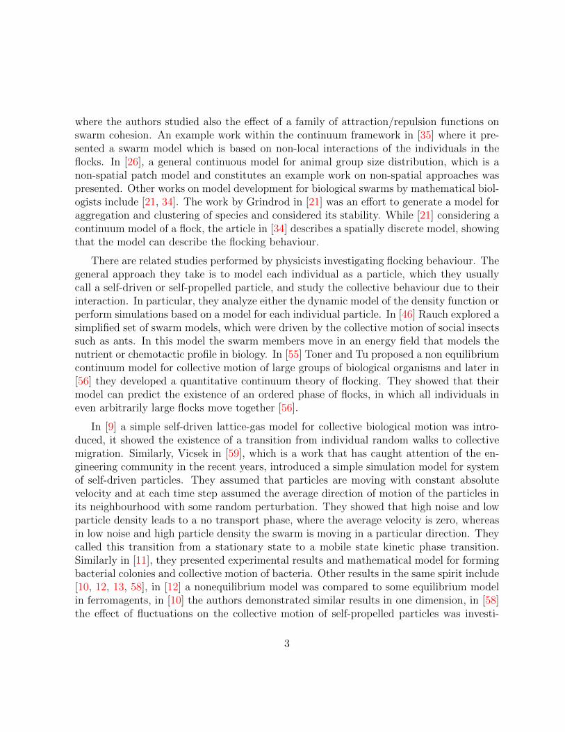
where the authors studied also the effect of a family of attraction/repulsion functions onswarm cohesion. An example work within the continuum framework in [35] where it pre-sented a swarm model which is based on non-local interactions of the individuals in theflocks. In [26], a general continuous model for animal group size distribution, which is anon-spatial patch model and constitutes an example work on non-spatial approaches waspresented. Other works on model development for biological swarms by mathematical biol-ogists include [21, 34]. The work by Grindrod in [21] was an effort to generate a model foraggregation and clustering of species and considered its stability. While [21] considering acontinuum model of a flock, the article in [34] describes a spatially discrete model, showingthat the model can describe the flocking behaviour.
There are related studies performed by physicists investigating flocking behaviour. Thegeneral approach they take is to model each individual as a particle, which they usuallycall a self-driven or self-propelled particle, and study the collective behaviour due to theirinteraction. In particular, they analyze either the dynamic model of the density function orperform simulations based on a model for each individual particle. In [46] Rauch explored asimplified set of swarm models, which were driven by the collective motion of social insectssuch as ants. In this model the swarm members move in an energy field that models thenutrient or chemotactic profile in biology. In [55] Toner and Tu proposed a non equilibriumcontinuum model for collective motion of large groups of biological organisms and later in[56] they developed a quantitative continuum theory of flocking. They showed that theirmodel can predict the existence of an ordered phase of flocks, in which all individuals ineven arbitrarily large flocks move together [56].
In [9] a simple self-driven lattice-gas model for collective biological motion was intro-duced, it showed the existence of a transition from individual random walks to collectivemigration. Similarly, Vicsek in [59], which is a work that has caught attention of the en-gineering community in the recent years, introduced a simple simulation model for systemof self-driven particles. They assumed that particles are moving with constant absolutevelocity and at each time step assumed the average direction of motion of the particles inits neighbourhood with some random perturbation. They showed that high noise and lowparticle density leads to a no transport phase, where the average velocity is zero, whereasin low noise and high particle density the swarm is moving in a particular direction. Theycalled this transition from a stationary state to a mobile state kinetic phase transition.Similarly in [11], they presented experimental results and mathematical model for formingbacterial colonies and collective motion of bacteria. Other results in the same spirit include[10, 12, 13, 58], in [12] a nonequilibrium model was compared to some equilibrium modelin ferromagents, in [10] the authors demonstrated similar results in one dimension, in [58]the effect of fluctuations on the collective motion of self-propelled particles was investi-
3
gated, and in [13] the effect of noise and dimensionality on the scaling behaviour of flocksof self-propelled particles was studied.
The field of coordinated multi-agent dynamical systems has become popular in the pastdecade in the engineering community as well. One of the earliest works in this field is thework by Reynolds [47] on simulation of a flock of birds in flight using a behavioural modelbased on few simple rules and only local interactions. Reynolds introduced three heuristicrules that led to flocking. here are three quotes from [47] that describe these rules:
1. Flock Centering: attempt to stay close to nearby flock mates.
2. Obstacle Avoidance: avoid collisions with nearby flock mates.
3. Velocity Matching: attempt to match velocity with nearby flock mates.
These three rules are also known as cohesion, separation and alignment rules in the liter-ature. The main problem with implementation or analysis of the above rules is that theyhave broad interpretations. The issue of how to interpret Reynolds rules was resolved afterpublication of more recent papers by Reynolds [48, 49].
Early work on swarm stability is given by Beni and coworkers in [31] and [4]. In [31]they considered a synchronous distributed control method for discrete one and two dimen-sional swarm structures and prove stability in the presence of disturbances using Lyapunovmethods. In [4] they considered a linear model and provided sufficient conditions for asyn-chronous convergence (without time delays) of the flocks to a synchronously achievableconfiguration.
Coordinated motion and distributed formation control of agents are important problemsin the multi-agent formation control literature. In systems under minimalistic assumptionsit might be difficult to achieve even simple formations. In [53] the authors consideredasynchronous distributed control and geometric pattern formation of multiple anonymousagents. Other important studies on cooperative control and coordination of swarms ofagents and in particular formation control of autonomous air or land vehicles using variousdifferent approaches can be found in [61, 43, 24, 3]. In [61] the authors considered coop-erative control and coordination of a group of holonomic mobile robots to capture/enclosea target by making group formations. Results of a similar nature using behaviour basedstrategy can be found also in [3], where they considered a strategy in which the formationbehaviour is integrated with other navigational behaviour and present both simulation andimplementation results for various types of formations and formation strategies. In [24],the authors described formation control strategies for autonomous air vehicles. They used
4
optimization and graph theory approach to find the best set of communication channelsthat will keep the aircraft in the desired formation.
Other work on formation control and coordination of multi-agent systems can be foundin [2, 14, 15, 17, 33, 36]. In [14, 15], a feedback linearization technique using only local in-formation for controller design to exponentially stabilize the relative distances of the robotsin the formation was proposed. Similarly, in [17, 36], the concept of control Lyapunov func-tions together with formation constraints was used to develop a formation control strategyand prove stability of the formation (formation maintenance). The results in [33], on theother hand, were based on using virtual leaders and artificial potentials for agent interac-tions in a group of agents for maintenance of a predefined group geometry. By using thesystem kinetic energy energy and the artificial potential energy as a Lyapunov functionclosed loop stability was shown. Moreover, a dissipative term was employed in order toachieve asymptotic stability of the formation. In [2], the results in [33] were extended tothe case in which the group is moving in a sampled gradient fields.
In comparison with continuous control which had been well studied before, there arenot many reports on the design of impulsive control for multi-agent systems with switchingtopologies. It has been proved that impulsive control approach is effective and robustin synchronization of chaotic systems and complex networks [63], and the advantage ofapplying impulsive control in a self-driven, communicating multi-agent systems is to reduceenergy and communication cost. We can imagine that a bird in a flock will not flap itswings all the time. Motivated by the above discussions, we consider the flocking/formationcontrol problem of multi-agent dynamical systems with switching topologies by hybridcontrol method, numerical examples and simulations are provided to illustrate the results.
The thesis is organized as follows:
Chapter 2 In this chapter, we give a general background to multi-agent system mod-elling, some basic concepts of graph theory are introduced and a particle-based frameworkis presented to describe our problem. Construction for potential functions is investigatedin detail.
Chapter 3 In this chapter, we discuss the continuous models for flocking for multi-agentdynamical systems. The concepts of fixed and switching topologies are introduced, a virtualleader is applied into our flocking algorithm and successfully leads to flocking. Stabilityproblem for free-flocking is discussed in detail, furthermore, models for constrained-flockingare also provided.
Chapter 4 In this chapter, we extend the existing continuous flocking models withimpulsive control and delay, techniques for stability of impulsive systems are used to analyze
5

the asymptotic stability of the equilibrium of our hybrid flocking models, additionallyalgorithms for flocking with dynamical obstacle avoidance capability are proposed.
Chapter 5 In this chapter, we give our conclusions and directions for future work.
6
Chapter 2
Muti-Agent Dynamical SystemModelling
In order to model multi-agent dynamical systems and study the flocking behaviour andinterconnection between agents in the model, one can begin by defining agents to havesensory capabilities (i.e., to sense position or velocity of other agents or sense environmen-tal characteristics), processing ability (a brain or an on-board computer), the ability tocommunicate or exchange information and the ability to take actions via actuators [23].Physical agent characteristics along with agent motion dynamics and its sensory and pro-cessing capabilities constrain how the agent can move in its environment and the rates atwhich it can sense and act in spatially distributed areas and interact with the other agents.
Regardless, it is useful to think of the agents as nodes, and arcs between nodes asrepresenting abilities to sense or communicate with other agents. The existence of an arcmay depend on sensing range of agents, the properties of the environment, communicationnetwork and link imperfections, along with local agent abilities and goals. One can view amulti-agent dynamical system as a set of such communicating agents that work collectivelyto solve a task.
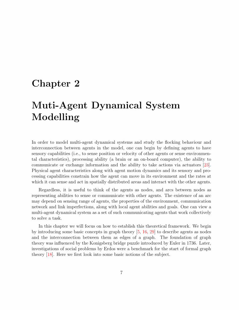
In this chapter we will focus on how to establish this theoretical framework. We beginby introducing some basic concepts in graph theory [5, 16, 29] to describe agents as nodesand the interconnection between them as edges of a graph. The foundation of graphtheory was influenced by the Konigsberg bridge puzzle introduced by Euler in 1736. Later,investigations of social problems by Erdos were a benchmark for the start of formal graphtheory [18]. Here we first look into some basic notions of the subject.
7
6
4 5
3 2
1
e1
e2
e5
e6
e4
e3
e7
(a)
6
4 5
3 2
1
e1
e2
e5
e6 e4
e3e7
e8
(b)
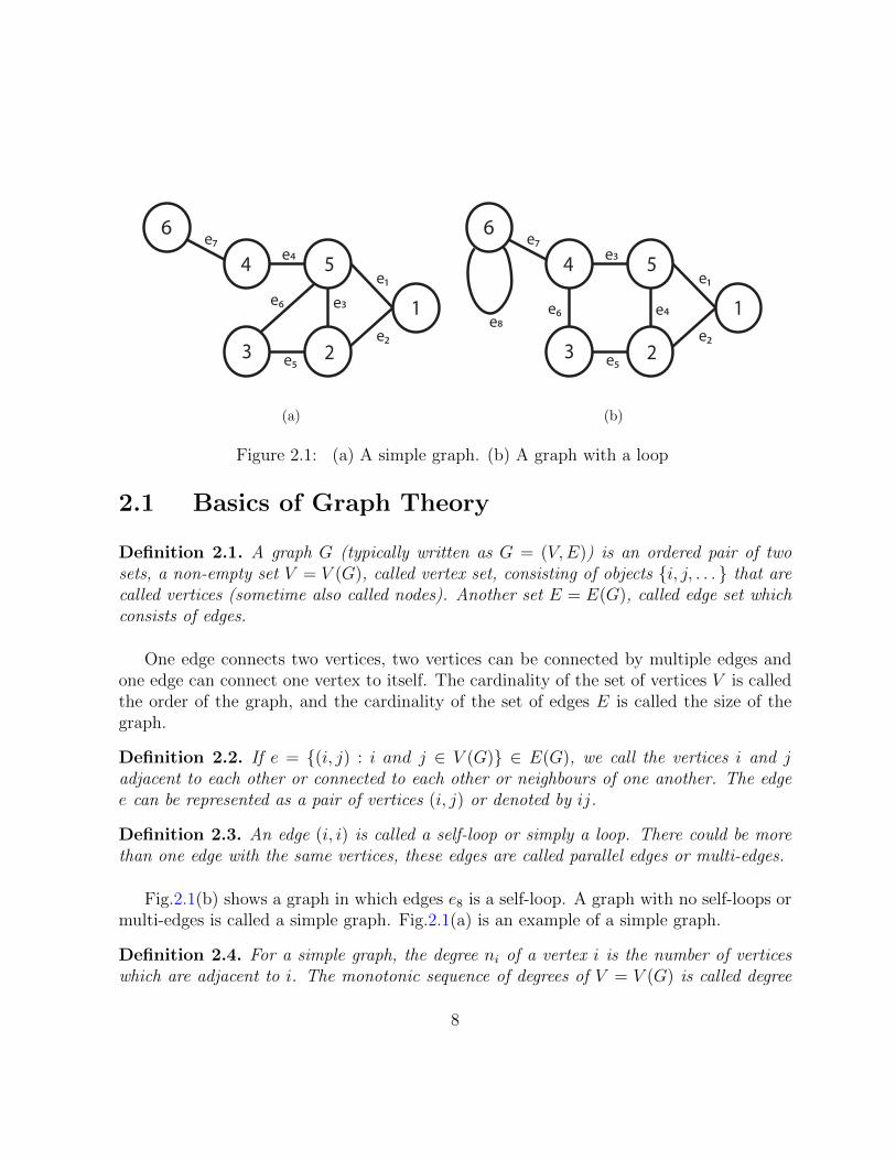
Figure 2.1: (a) A simple graph. (b) A graph with a loop
2.1 Basics of Graph Theory
Definition 2.1. A graph G (typically written as G = (V,E)) is an ordered pair of twosets, a non-empty set V = V (G), called vertex set, consisting of objects i, j, . . . that arecalled vertices (sometime also called nodes). Another set E = E(G), called edge set whichconsists of edges.
One edge connects two vertices, two vertices can be connected by multiple edges andone edge can connect one vertex to itself. The cardinality of the set of vertices V is calledthe order of the graph, and the cardinality of the set of edges E is called the size of thegraph.
Definition 2.2. If e = (i, j) : i and j ∈ V (G) ∈ E(G), we call the vertices i and jadjacent to each other or connected to each other or neighbours of one another. The edgee can be represented as a pair of vertices (i, j) or denoted by ij.
Definition 2.3. An edge (i, i) is called a self-loop or simply a loop. There could be morethan one edge with the same vertices, these edges are called parallel edges or multi-edges.
Fig.2.1(b) shows a graph in which edges e8 is a self-loop. A graph with no self-loops ormulti-edges is called a simple graph. Fig.2.1(a) is an example of a simple graph.
Definition 2.4. For a simple graph, the degree ni of a vertex i is the number of verticeswhich are adjacent to i. The monotonic sequence of degrees of V = V (G) is called degree
8
6
4 5
3 2
1
e1
e2
e5
e6
e4
e3
e7
(a)
6
4 5
2
1
e1
e2
e6
e4
e3
e7
(b)
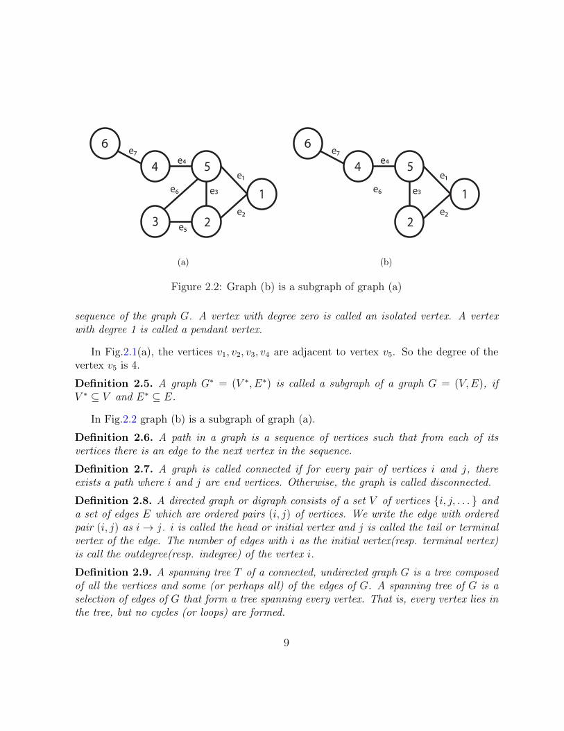
Figure 2.2: Graph (b) is a subgraph of graph (a)
sequence of the graph G. A vertex with degree zero is called an isolated vertex. A vertexwith degree 1 is called a pendant vertex.
In Fig.2.1(a), the vertices v1, v2, v3, v4 are adjacent to vertex v5. So the degree of thevertex v5 is 4.
Definition 2.5. A graph G∗ = (V ∗, E∗) is called a subgraph of a graph G = (V,E), ifV ∗ ⊆ V and E∗ ⊆ E.
In Fig.2.2 graph (b) is a subgraph of graph (a).
Definition 2.6. A path in a graph is a sequence of vertices such that from each of itsvertices there is an edge to the next vertex in the sequence.
Definition 2.7. A graph is called connected if for every pair of vertices i and j, thereexists a path where i and j are end vertices. Otherwise, the graph is called disconnected.
Definition 2.8. A directed graph or digraph consists of a set V of vertices i, j, . . . anda set of edges E which are ordered pairs (i, j) of vertices. We write the edge with orderedpair (i, j) as i→ j. i is called the head or initial vertex and j is called the tail or terminalvertex of the edge. The number of edges with i as the initial vertex(resp. terminal vertex)is call the outdegree(resp. indegree) of the vertex i.
Definition 2.9. A spanning tree T of a connected, undirected graph G is a tree composedof all the vertices and some (or perhaps all) of the edges of G. A spanning tree of G is aselection of edges of G that form a tree spanning every vertex. That is, every vertex lies inthe tree, but no cycles (or loops) are formed.
9
2.1.1 Adjacency Matrix
The adjacency matrix of a graph G of n vertices is a n× n matrix where the non-diagonalentry aij is the number of edges connecting from vertex i to vertex j, and the diagonalentry aii, depending on the convention, is either once or twice the number of edges(loops)from vertex i to itself. Undirected graphs often use the former convention of counting loopstwice, whereas directed graphs typically use the latter convention. If a graph is undirected,the adjacency matrix is symmetric, and therefore has a complete set of real eigenvaluesand an orthogonal eigenvector basis. The set of eigenvalues of the adjacency matrix of agraph is the spectrum of the graph.
Adjacency Matrix: The matrix A = [aij] with the form
aij =
1, if ij is an edge
0, otherwise
is the adjacency matrix of the most common simple undirected graph.
Following is the adjacency matrix of the graph in Fig.2.1(b)0 1 0 0 1 01 0 1 0 1 00 1 0 1 0 00 0 1 0 1 11 1 0 1 0 00 0 0 1 0 1
2.1.2 Graph Laplacian
The graph Laplacian matrix is important for analyzing the graph’s structure, (which laterwill be useful in analysis of velocity matching in multi-agent dynamical systems). It isdefined in the following way:
Laplacian Matrix: The matrix L = [aij] with the form
aij =
ni, if i = j
−1, if ij is an edge
0, otherwise
10
is called the Laplacian matrix of a graph, where ni denotes the degrees of the vertices i.Following is an example of the corresponding Laplacian of the graph in Fig.2.1(b)
2 −1 0 0 −1 0−1 3 −1 0 −1 00 −1 2 −1 0 00 0 −1 3 −1 −1−1 −1 0 −1 3 00 0 0 −1 0 1
Relationship between adjacency matrix and Laplacian martix
For a graph G, let D be the diagonal matrix with entries which are the degrees ofvertices, i.e.,
D(i, j) =
ni, if i = j
0, otherwise
where ni denotes the degrees of the vertices i. The relation between the adjacency matrixA and the graph Laplacian L is
L = D − A
Laplacian matrix L always has a right eigenvector of 1n = (1, . . . , 1)T associated witheigenvalue λ1 = 0. The following lemma from [38] summarizes the basic properties ofgraph Laplacians:
Lemma 2.1. Let G(V,E) be an undirected graph of order n with a non-negative adjacencymatrix A = AT . Then, the following statements hold:
1. L is a positive semidefinite matrix that satisfies the follow sum-of-squares (SOS)property:
zTLz =1
2
∑i,j∈E
aij(zj − zi)2, z ∈ Rn;
2. The graph G has c ≥ 1 connected components if and only if rank(L) = n − c.Particularly, G is connected if and only if rank(L) = n− 1;
3. Let G be a connected graph, then
λ2(L) = minz⊥1nzTLz
‖z‖2> 0,
11
Proof. All three results are well-known in the field of algebraic graph theory and theirproofs can be found in Godsil and Royle [25].
The quantity λ2(L) is known as algebraic connectivity of a graph [20]. Particularly, weuse m-dimensional graph Laplacians defined by
L = L⊗ 1m
where ⊗ denotes the Kronecker product. This multi-dimensional Laplacian satisfies thefollowing SOS property:
zT Lz =1
2
∑(i,j)∈E
aij‖zj − zi‖2, z ∈ Rmn
where z = (z1, z2, . . . , zn)T and zi ∈ R for all i. Matrix L can be viewed as the Laplacianof a graph with adjacency matrix A = A⊗ 1m.
We can use the graph Laplacian to evaluate the graph/network connectivity mainte-nance. We know that the link/connection between vertex i and vertex j is maintainedif ij ∈ e, otherwise this link is considered to be broken. For graph connectivity, a dy-namic graph G(V,E) is said to be connected at time t only if there exists a path betweenany two vertices at time t. To analyze the connectivity of the graph/network, we define
c(t) = Rank(L(t))n−1 ; if 0 ≤ c(t) < 1, the network is broken; if c(t) = 1, the network is con-
nected. This property of the Laplacian is very useful to analyze the flocking behaviour ofmulti-agent dynamical systems.
2.1.3 Particle-Based System
After introducing the basic knowledge of graph theory, now we need to set up a theoreticalmodel to analyze the flocking behaviour of multi-agent dynamical systems. We propose aparticle-based model assuming agents in the system are self-driven or self-propelled parti-cles, and possess sensing ability to perceive the position and velocity information of otheragents which are within their interaction/communication range. The concept of spatialneighbour of an agent is also introduced.
Let G = (V,E) be a graph and ri ∈ Rm denote the position of agent i for all i ∈ V .The vector r = (r1, . . . , rn) ∈ Rmn is called the configuration of all nodes of the graph. Aframework (or structure) is a pair (G,r) that consists of a graph and the configuration ofits nodes.
12
Interation Range
R
i
1
2
3
4
5
6
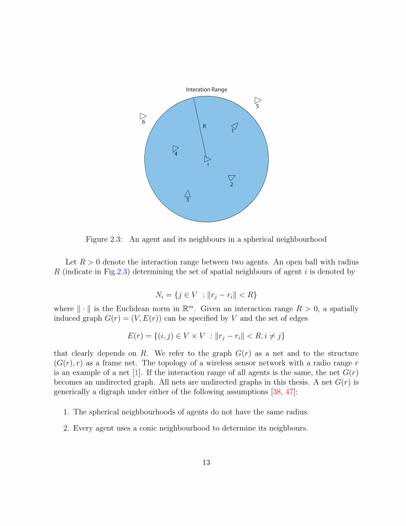
Figure 2.3: An agent and its neighbours in a spherical neighbourhood
Let R > 0 denote the interaction range between two agents. An open ball with radiusR (indicate in Fig.2.3) determining the set of spatial neighbours of agent i is denoted by
Ni = j ∈ V : ‖rj − ri‖ < R
where ‖ · ‖ is the Euclidean norm in Rm. Given an interaction range R > 0, a spatiallyinduced graph G(r) = (V,E(r)) can be specified by V and the set of edges
E(r) = (i, j) ∈ V × V : ‖rj − ri‖ < R, i 6= j
that clearly depends on R. We refer to the graph G(r) as a net and to the structure(G(r), r) as a frame net. The topology of a wireless sensor network with a radio range ris an example of a net [1]. If the interaction range of all agents is the same, the net G(r)becomes an undirected graph. All nets are undirected graphs in this thesis. A net G(r) isgenerically a digraph under either of the following assumptions [38, 47]:
1. The spherical neighbourhoods of agents do not have the same radius.
2. Every agent uses a conic neighbourhood to determine its neighbours.
13

2.2 Vicsek’s Discrete Model
Among the first groups of physicists who studied flocking from a theoretical perspectivewere Vicsek. In [57] Vicsek introduced a simple discrete time model with a novel typeof dynamics in order to investigate the emergence of self-ordered motion in systems ofparticles with biologically motivated interaction. In Vicsek’s model, particles were drivenwith a constant absolute velocity and at each time step assumed the average direction ofmotion of the particles in their neighbourhood with some random perturbation in analogywith the temperature. Numerical simulations were provided to indicate that this modelresults in rich, realistic dynamics, including a kinetic phase transition. Vicsek’s work has animportant influence on the later researches of flocking for multi-agent systems since flockingis the kind of coordinated behaviour which combines both position (phase) transition andvelocity alignment.
The model is carried out in a square shaped cell of linear size L with periodic boundaryconditions. The particles are represented by points moving continuously on this plane. Weuse the interaction range R as the unit to measure distances (R = 1), while the time unit∆t = 1 is the time interval between two updates of the velocity directions and positions.In most of the simulations we use the simplest initial conditions:
1. At time t = 0, all particles’ position are randomly distributed in the plane.
2. At time t = 0, all particles have the same absolute velocity v.
3. At time t = 0, the directions θ of all particles’ velocity are randomly distributed.
The velocities v of the particles are determined simultaneously at each time step, and theposition of the ith particle updates according to a simple rule which can be described asfollow:
xi(t+ 1) = xi(t) + vi(t)∆t
where the velocity of a particle vi(t + 1) is constructed to have an absolute value v and adirection given by the angle θ(t+ 1). This angle is given by the following expression:
θ(t+ 1) =< θ(t) >R +∆θ
where < θ(t)R > denotes the average direction of the velocities of particles (includingparticle i) which are in a circle of radius R centering at the given particle. The average
direction is given by the angle arctan[<sin(θ(t))>R<cos(θ(t))>R
] and ∆θ is a random number chosen with
14
a uniform probability from the interval [−η/2, η/2]. Thus the term ∆θ represents noisewhich we shall use as a temperaturelike variable. Correspondingly, there are three freeparameters for a given system size: η, ρ, and v where v is the distance a particle travelsbetween two updates, and ρ = v/L2 is the density.
We need to investigate the nontrivial behaviour of the transport properties as the twobasic parameters of the model, the noise η and the density ρ are varied. We use v = 0.2in the simulations, as v → 0 the particles do not move. For v → ∞ the particles becomecompletely mixed between two updates, and this limit corresponds to the so-called mean-field behaviour of a ferromagnet. We use v = 0.2 for which the particles always interactwith their actual neighbours and move fast enough to change the configuration after afew updates of the directions. According to the simulations, in a range of the interval(0.03 < v < 0.3), the actual value of v does not affect the results. Figures2.4(a)-(d)demonstrate the velocity fields during runs with various selections for the value of theparameter ρ and η. The actual velocity of a particle is indicated by a small arrow. (a) Att=0 the positions and the directions of velocities are distributed randomly. (b) For smallnoise the particles tend to form groups moving coherently in random directions. (c) Athigher noise the directions of velocities are distributed randomly at t=0 and (d) After 100time steps the particles still move randomly in random direction.
The emergence of cooperative motion in this model has analogies with the appearanceof spatial order in equilibrium systems. This fact and the simplicity of this model suggeststhat with appropriate modifications, the theoretical methods for describing critical phe-nomena may be applicable to other kind of equilibrium phase transition such as flockingbehaviour. A rigorous proof of convergence by Jadbabaie [30] for Vicseks model was givenin Appendix A.
2.3 Double Integrator Agents
In this section we consider a double integrator model for agents. As in the last section, wehave introduced some basic background of modelling and Vicsek’s discrete velocity con-sensus model, here we will propose the model of double integrator agents and a systematicmethod is provided for construction of inter-agent potential function to investigate theflocking behaviour for multi-agent dynamical systems.
15
−0.5 0 0.5 1 1.5 2 2.5−0.5
0
0.5
1
1.5
2
2.5
(a)
0 0.5 1 1.5 2 2.5 30
0.5
1
1.5
2
2.5
(b)
−0.5 0 0.5 1 1.5 2 2.5−0.5
0
0.5
1
1.5
2
2.5
(c)
2.5 3 3.5 4 4.5 5 5.5 62.5
3
3.5
4
4.5
5
5.5
(d)
Figure 2.4: (a) low noise at t=0 (b) low noise after 30 time steps (c) high noise at t=0 (d)high noise after 100 time steps
16
2.3.1 Equation of Motion
We consider a system consists of N interconnecting agents, each with point mass dynamicsgiven by
ri = vi
vi = 1Miui
(2.1)
where ri ∈ Rn is the position, vi ∈ Rn is the velocity, Mi is the mass and ui ∈ Rn is the(force) control input for the ith agent. The above equations imply that ui = Miri (forceis mass times acceleration). Integrating acceleration once we get velocity, twice and weget position; hence, we use the term “double integrator model.” It is assumed that allagents know their own dynamics. For some organisms like bacteria that move in highlyviscous environments it can be assumed that Mi = 0. If a velocity damping term is usedin ui, we obtain the model proposed by Olfati-Saber [45] which will be studied in Chapter3 (assuming that Mi = 1).
2.3.2 Potential Function Design
Given the agent dynamics in (2.3.1), in this section we will discuss developing controlalgorithms for obtaining coordinated behaviour for multi-agent dynamical systems. Wewill solve this problem by using a potential function based approach. We assume allindividuals in the system move simultaneously and know the exact relative position of theother individuals. Let rT = [rT1 , r
T2 . . . r
Tn ] ∈ Rnn denote the vector of concatenated states
of all the agents. In this section the control input ui of individual i will have the form
ui = −∇riJ(r)
where J : Rnn → R is a potential function which represents the interaction (i.e., theattraction and repulsion relationship) between the individual agents and needs to be chosenby the designer based on the flocking application under consideration and the desiredbehaviour from the system. We will discuss which properties the potential functions shouldsatisfy for different problems and present results for some potential functions.
Aggregation is one of the most basic behaviour seen in flocks in nature (such as insectcolonies) and is sometimes the initial phase in collective tasks performed by a flock. Below,we discuss how to achieve aggregation for the single integrator model in (2.3.1). If onlysimple aggregation is desired from the multi-agent dynamical system, then the potential
17
function J can be selected as J(r) = Jaggregation(r) where
Jaggregation =n−1∑i=1
n∑j=i+1
[Ja(‖ri − rj‖)− Jr(‖ri − rj‖)].
Here, Ja : R+ → R represents the attraction component, whereas Jr : R+ → R representsthe repulsion component of the potential function. Although not the only choice, the abovepotential function is very intuitive since it represents an interplay between attraction andrepulsion components. Note also that it is based only on the relative distances betweenthe agents and not the absolute agent positions.
Given the above type of potential function, the control input of individual i, j =1, . . . , N can be calculated as
ui = −n∑
j=1,j 6=i
[∇riJa(‖ri − rj‖)−∇riJr(‖ri − rj‖)]
Note that since vi = ui, the motion of the individual is along the negative gradient andleads to a descent motion towards a minimum of the potential function J . Moreover, sincethe function Ja(‖r‖) and Jr(‖r‖) create a potential field of attraction and repulsion, respec-tively, around each individual, the above property restricts the motion of the individualstoward each other along the gradient of these potentials (i.e., along the combined gradientfield of Ja(‖r‖) and Jr(‖r‖)).
One can show that, because of the chain rule and the definition of the functions Ja andJr, the equalities
∇rJa(‖r‖) = rga(‖r‖)∇rJr(‖r‖) = rgr(‖r‖)
are always satisfied for some some function ga : R+ → R and gr : R+ → R. Here ga : R+ →R+ represents the attraction term, whereas gr : R+ → R+ represents the repulsion term.Note also that the combined term −rga(‖r‖) represents the actual attraction whereasthe combined term rgr(‖r‖) represents the actual repulsion, and they both act on theline connecting the two interaction individuals, but in opposite directions. The vectorr determines the alignment, it guarantees that the interaction vector is along the lineon which r is located), and it also affects the magnitude of the attraction and repulsioncomponents. The terms ga(‖r‖) and gr(‖r‖), on the other hand, affect correspondingly
18
only the magnitude of the attraction and repulsion, whereas their difference determine thedirection of the interaction along vector r. Let’s define the function g(·) as
g(r) = −r[ga(‖r‖)− gr(‖r‖)]. (2.2)
We call the function g(·) an attraction/repulsion function and assume that on large dis-tances attraction dominates, while on short distances repulsion dominates, and that thereis a unique distance at which the attraction and the repulsion balance. In other words, weassume that g(·) satisfies the following assumptions.
Definition 2.10. The function g(·) in (2.2) and the corresponding ga(·) and gr(·) are suchthat there exist a unique distance d at which we have ga(d) = gr(d). Moreover, we havega(‖r‖) > gr(‖r‖) for ‖r‖ > d and gr(‖r‖) > ga(‖r‖) for ‖r‖ < d.
Moreover for the attraction/repulsion function g(·) defined as above we have g(r) =−g(−r), in other words, the above g(·) functions are odd. This is an important feature ofthe g(·) functions that lead to reciprocity in the inter-agent relations and interactions.
Non-smooth Potential Fucntion
In order to satisfy the above assumptions, the potential function designer should choosethe attraction and repulsion potential such that the minimum of Ja(‖ri − rj‖) occurs on‖ri − rj‖ = 0, whereas the minimum of −Jr(‖ri − rj‖) occurs on ‖ri − rj‖ → ∞, andthe minimum of the combined Ja(‖ri − rj‖) − Jr(‖ri − rj‖) occurs at ‖ri − rj‖ = d. Inother words, at ‖ri − rj‖ = d the attraction/repulsion potential between two interactingindividuals has a global minimum, however, when there are more than two individuals, theminimum of the combined potential does not necessarily occur at ‖ri−rj‖ = d for all j 6= i.Moreover, there exist a family of minima. So we can view J(r) as the potential average ofthe multi-agents system, whose value depends on the inter-individual distances (such thatit’s high when the agents are either far from each other or too close to each other) and themotion of all the agents is towards a unique global minimum energy configuration.
One potential function which satisfies the above conditions, including Assumption 2.10,and has been used in Tanner’s model [28] is:
Jij =
1
‖ri−rj‖2 + log‖ri − rj‖2, ‖ri − rj‖ < R
VR ‖ri − rj‖ ≥ R(2.3)
where R denotes the interaction range between two agents and VR = 1/R2 + logR2 is apositive constant. Its corresponding attraction/repulsion function can be calculates as
19
r
uij
(a)
J
r
Interaction Range
Global Minimum
ij
(b)
Figure 2.5: (a) A Discontinuous Attraction/Repulsion Function. (b) A Non-SmoothPotential Function with R=2
uij =−2
‖ri − rj‖3+
2
‖ri − rj‖(2.4)
which is indicated in Fig.2.5(a). We can see that the attraction/repulsion functionis zero at r = 1 which is the global minimum of the corresponding potential function,indicating that the attraction and repulsion are balance at this equilibrium position. Alsonotice that due to the property that the potential function is not smooth at R = 2, so inthe Fig.2.5(a) of the attraction/repulsion function we can see there is a jump at R = 2,which implies that the interaction between two agents is suddenly disappear when they areout of their interaction range. Moreover, from Fig.2.5(b) we notice that this non-smoothpotential function is not differentiable and goes to infinity at 0, which means we need toapply an unbounded repulsive force to avoid collision between two agents.
20
Smooth Potential Function
The non-smooth potential function introduced in Tanner’s model is not differentiable at 0,this is due to the fact that the map ‖r‖ is not differentiable at r = 0. Moreover, we want toconstruct a potential function with a finite cut-off at R, which mean the potential functionis zero for all r ≥ R. Hence, in order to construct a new smooth potential function with afinite cut-off, we need to introduce σ-Norms and Bump functions.
Definition 2.11. The σ-norm of a vector is a map Rm → R+ defined as
‖r‖σ =1
ε[√
1 + ε‖r‖2 − 1]
with a parameter ε > 0 and a gradient σε(r) = ∇‖r‖σ given by
σε(r) =r√
1 + ε‖r‖2=
r
1 + ε‖r‖σ
Notice the map ‖r‖σ is differentiable everywhere whereas ‖r‖ is not differentiable atr = 0. Later this property of σ-norms is used for construction of smooth collective potentialfunctions for multi-agent dynamical system.
Definition 2.12. A bump function is a scalar function ph(r) that smoothly varies between0 and 1.
Here we use bump functions for construction of smooth potential functions with finitecut-offs, one possible choice is the following bump function introduced in [50]
ph(r) =
1, r ∈ [0, h)12[1 + cos(π r−h
1−h)], r ∈ [h, 1]
0 otherwise
(2.5)
where h ∈ (0, 1). One can show that ph(r) is a C1-smooth function with the property thatph′(r) = 0 over the interval [1,∞) and |ph′(r)| is uniformly bounded in r. A example of
(2.5) with h = 0.2 is given is Fig.2.6
A collective potential function ψ(r) is a smooth version of a deviation energy function[45]with a scalar pairwise potential that has a finite cut-off. This means that there exists afinite interaction range R > 0 such that ψ′(r) = 0,∀r > R. This feature turns out to bethe fundamental source of scalability of our flocking algorithms. A common approach to
21
r
ph(r)
Figure 2.6: A Bump Function with h=0.2
create a pairwise potential with a finite cut-off is “soft cutting” in which a pairwise poten-tial is multiplied by a bump function [38]. Here we use an alternative approach by softlycutting attraction/repulsion functions and then using their integrals as pairwise potentials.This way the derivative of the bump function never appears in the attraction/repulsionfunction, and thereby a negative bump in the action function near r = R is avoided.
Let ψ(r) : R+ → R+ be an attraction/repulsion pairwise potential function with aglobal minimum at r = d and a finite cut-off at R. Then the following function
ϕ(r) =1
2
n∑i=1
∑j 6=i
ψ(‖ri − rj‖ − d)
is a collective potential function that is not differentiable at singular configurations inwhich two distinct nodes coincide, or ri = rj. To resolve this problem, we use the set ofalgebraic constraints that are written in terms of σ-norms as
‖ri − rj‖σ = dα, ∀j ∈ Ni(r)
22
where Ni(r) denotes all the neighbours of agent i, dα = ‖d‖σ. These constraints induce asmooth collective potential function of the form:
V (r) =1
2
∑i
∑j 6=i
ψα(‖ri − rj‖σ) (2.6)
where ψα(r) is a smooth pairwise attraction/repulsion potential with a finite cut-off atrα = ‖r‖σ and a global minimum at r = dα.
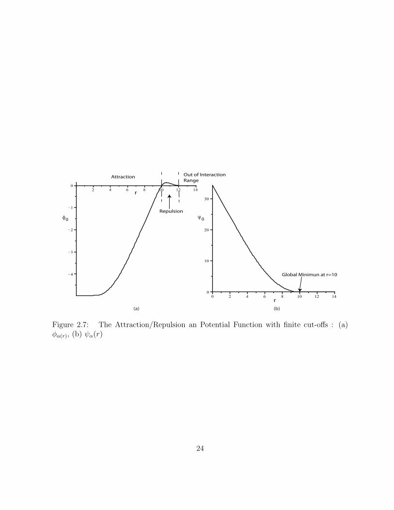
To construct a smooth pairwise potential with finite cut-off, we integrate an attrac-tion/repulsion function φα(r) that vanishes for all r ≥ Rα. Define this attraction/repulsionfunction as
φα(r) = ph(r
Rα
)φ(r − dα) (2.7)
φ(r) =1
2[(a+ b)σ1(r + c) + (a− b)] (2.8)
where σ1(r) = r/√
1 + r2 and φ(r) is an uneven sigmoidal function with parametersthat satisfy 0 < a ≤ b, c = |a − b|/
√4ab to guarantee φ(0) = 0. The pairwise attrac-
tion/repulsion potential ψα(r) is defined as
ψα(r) =
∫ r
dα
φα(s)ds (2.9)
Functions φα and ψα(r) are indicated in Fig.2.7
23
Global Minimun at r=10
r
Attraction
Repulsion
Out of Interaction
Range
r
(a) (b)
ф Ψα α
Figure 2.7: The Attraction/Repulsion an Potential Function with finite cut-offs : (a)φα(r), (b) ψα(r)
24
Chapter 3
Flocking via Continuous Control
In last chapter we propose a double integrator model, we consider a system consists of Ninteracting agents with point mass dynamics given by
ri = vi
vi = 1Miui
(3.1)
where ri ∈ Rn is the position, vi ∈ Rn is the velocity, here we assume the mass Mi of everyagent in the model to be 1. In this chapter we will focus on using the potential functionand navigational feedback(a global objective of all the agents) to design the term ui tocontrol the agents in order to achieve the flocking phenomenon. One essential rule whichleads to flocking is that our control algorithms have to maintain the network connectivityof the system, which means all agents in the system can interact with at least one of itsneighbours. Hence, in this chapter we will first give the definition of α-Lattices which isconvenient for us to analyze the formation of the flocks, then we will provide a control ruleui without any navigational feedback for both fixed topologies and switching topologies. Wewill show that navigational feedback is necessary to avoid fragmentation of the flock. Thenwe will investigate the model proposed by Olfati-Saber [45] which includes a navigationalfeedback in the control input term that successfully lead to flocking. Stability analysis forOlfati-Saber’s model is provided and time delay and obstacle avoidance ability of agentsare also considered.
25
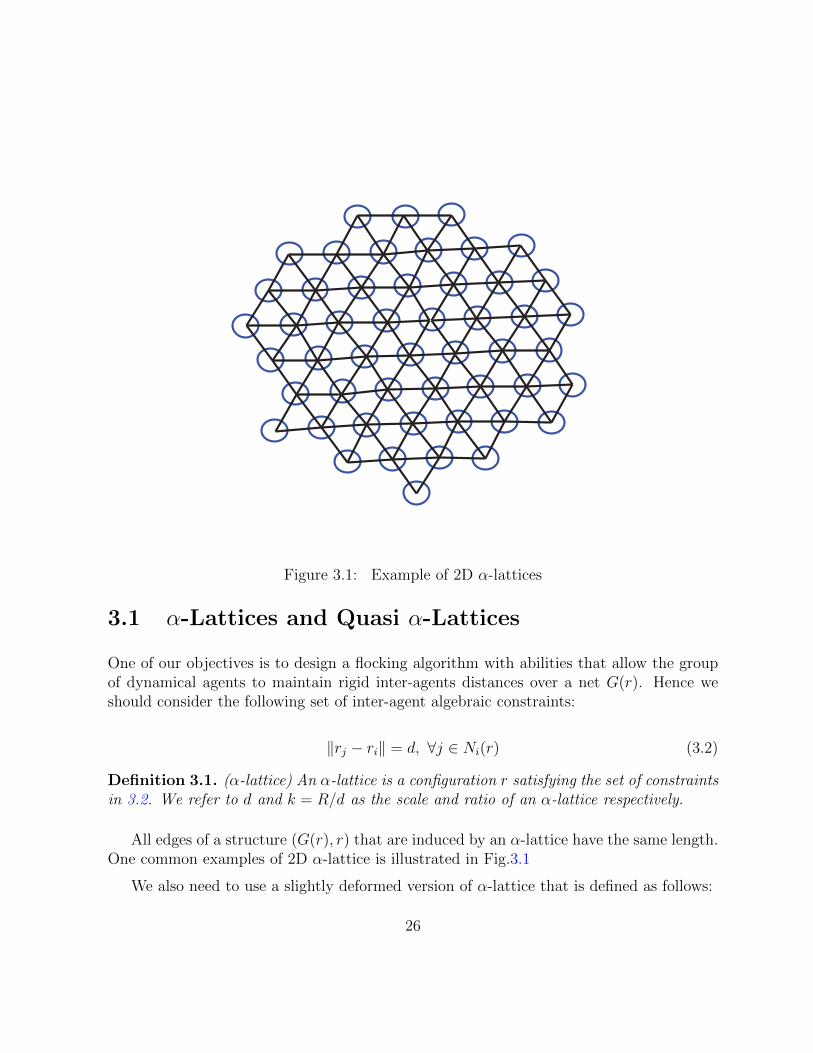
Figure 3.1: Example of 2D α-lattices
3.1 α-Lattices and Quasi α-Lattices
One of our objectives is to design a flocking algorithm with abilities that allow the groupof dynamical agents to maintain rigid inter-agents distances over a net G(r). Hence weshould consider the following set of inter-agent algebraic constraints:
‖rj − ri‖ = d, ∀j ∈ Ni(r) (3.2)
Definition 3.1. (α-lattice) An α-lattice is a configuration r satisfying the set of constraintsin 3.2. We refer to d and k = R/d as the scale and ratio of an α-lattice respectively.
All edges of a structure (G(r), r) that are induced by an α-lattice have the same length.One common examples of 2D α-lattice is illustrated in Fig.3.1
We also need to use a slightly deformed version of α-lattice that is defined as follows:
26
Definition 3.2. (quasi α-lattice) A quasi α-lattice is a configuration r satisfying the fol-lowing set of inequality constraints:
−δ ≤ ‖rj − ri‖ − d ≤ δ, ∀(i, j) ∈ E(r)
where δ << d is the edge-length uncertainty, d is the scale and k = r/d is the ratio of thequasi α-lattice.
3.2 Flocking Without Navigational Feedback
In this section we will study a well-known model without navigational feedback which isproposed by Tanner in [54] in 2003. In this model Tanner used a damping term and anartificial potential function which describes the attractive and repulsive behaviour betweenagents in the system. The motion of each agent is determined by two factors:
1. Attraction to the other agents over long distances.
2. Repulsion from the other agents over short distances.
Tanner’s model can be described as follows:ri = vi
vi = ui i = 1, . . . , N
The control input can be divided into two components:
ui = ai + αi.
The first component ai is attributed to an artificial potential function Vi, which dependson the relative position information between agent i and its neighbours. The second com-ponent αi regulates the velocity vectors of agent i to the average of that of its neighbours.
And the potential function is defined as follows:
Vij =
1
‖rij‖2 + log ‖rij‖2, ‖rij‖ < R
VR, ‖rij‖ ≥ R
27
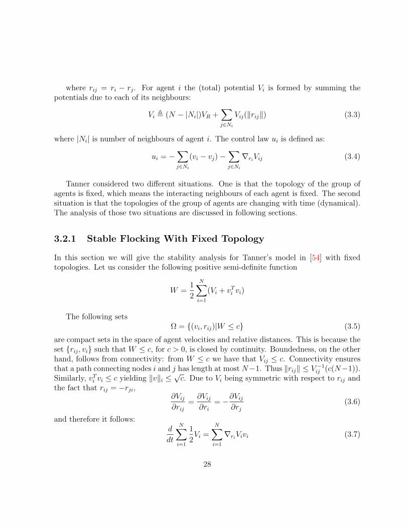
where rij = ri − rj. For agent i the (total) potential Vi is formed by summing thepotentials due to each of its neighbours:
Vi , (N − |Ni|)VR +∑j∈Ni
Vij(‖rij‖) (3.3)
where |Ni| is number of neighbours of agent i. The control law ui is defined as:
ui = −∑j∈Ni
(vi − vj)−∑j∈Ni
∇riVij (3.4)
Tanner considered two different situations. One is that the topology of the group ofagents is fixed, which means the interacting neighbours of each agent is fixed. The secondsituation is that the topologies of the group of agents are changing with time (dynamical).The analysis of those two situations are discussed in following sections.
3.2.1 Stable Flocking With Fixed Topology
In this section we will give the stability analysis for Tanner’s model in [54] with fixedtopologies. Let us consider the following positive semi-definite function
W =1
2
N∑i=1
(Vi + vTi vi)
The following setsΩ = (vi, rij)|W ≤ c (3.5)
are compact sets in the space of agent velocities and relative distances. This is because theset rij, vi such that W ≤ c, for c > 0, is closed by continuity. Boundedness, on the otherhand, follows from connectivity: from W ≤ c we have that Vij ≤ c. Connectivity ensuresthat a path connecting nodes i and j has length at most N−1. Thus ‖rij‖ ≤ V −1ij (c(N−1)).Similarly, vTi vi ≤ c yielding ‖v‖i ≤
√c. Due to Vi being symmetric with respect to rij and
the fact that rij = −rji,∂Vij∂rij
=∂Vij∂ri
= −∂Vij∂rj
(3.6)
and therefore it follows:d
dt
N∑i=1
1
2Vi =
N∑i=1
∇riVivi (3.7)
28
Theorem 3.1. (Tanner et al.(2003) [54]) Consider a system of N mobile agents withdynamics (3.2), each steered by control law (3.4) and assume that the graph is connected.Then all agent velocity vectors become asymptotically the same, collisions between inter-connected agents are avoided and the system approaches a configuration that minimizes allagent potentials.
Proof. Taking the time derivative of W , we have:
W =1
2
N∑i=1
Vi −N∑i=1
vTi (∑j∈Ni
(vi − vj) +∇riVi) (3.8)
due to the symmetric nature of Vij, this can be simplified to
W =N∑i=1
vTi ∇riVi −N∑i=1
vTi (∑j∈Ni
(vi − vj) +∇riVi)
= −N∑i=1
vTi∑j∈Ni
(vi − vj)
= −vT (L⊗ I2)v
where v is the state vector of all agent velocity vectors, L is the Laplacian of theneighbouring graph and ⊗ denotes the Kronecker matrix product. Writing the quadraticform explicitly,
W = −vTxLvx − vTy Lvy (3.9)
where vx and vy are the state vectors of the components of the agent velocities along xand y directions respectively. For a connected graph G, L is positive semidefinite andthe eigenvector associated with the single zero eigenvalue is 1. Thus W = 0 implies thatboth vx and vy belong to span1. This means that all agent velocities have the samecomponents and are therefore equal. It follows immediately that rij = 0, ∀(i, j) ∈ N ×N .Application of Lasalle’s invariance principle establishes convergence of system trajectoriesto S = v|W = 0. In S, the agent velocity dynamics become:
v = −
∇r1V1...
∇rNVN
= −(A⊗ I2)
...
∇rijVij...
(3.10)
29
where A is the adjacency matrix of the fixed graph. v can be expanded to
vx = −A[∇rijVij]x
vy = −A[∇rijVij]y
Thus, vx and vy belong in the range of the adjacency matrix A. For a connected graph,range(A) =span1⊥ and therefore
vx, vy ∈ span1⊥ (3.11)
In an invariant set within S,
vx, vy ∈ span1 ⇒ vx, vy ∈ span1. (3.12)
Combining (3.11) and (3.12), we have
vx, vy ∈ span1 ∩ span1⊥ = 0. (3.13)
Thus, in steady state agent velocities must not change. Furthermore, from (3.10) it followsthat in steady state the potential Vi of each agent i is minimized. Interconnected agentscannot collide since this will result in Vi → ∞ and the system departing Ω, which is acontradiction since Ω is positively invariant.
3.2.2 Stable Flocking With Switching Topologies
In this section, the topologies of the group of agents in the system are no longer fixed.We begin by proposing a similar theorem for flocking with switching topologies as in lastsection,
Theorem 3.2. (Tanner et al.(2003) [54]) Consider a system of N mobile agents withdynamics (3.2), each steered by control law (3.4) and assume that the neighbouring graph isconnected. Then all pairwise velocity differences converge asymptotically to zero, collisionsbetween the agents are avoided, and the system approaches a configuration that minimizesall agent potentials.
The proof for flocking with switching topologies is similar to the case of fixed topologyand is omitted here, a detailed proof given by Tanner can be found in [54].
One thing that needs to be mentioned is that in both cases of Tanner’s model, an im-portant assumption which must be satisfied for successful flocking is that the neighbouring
30
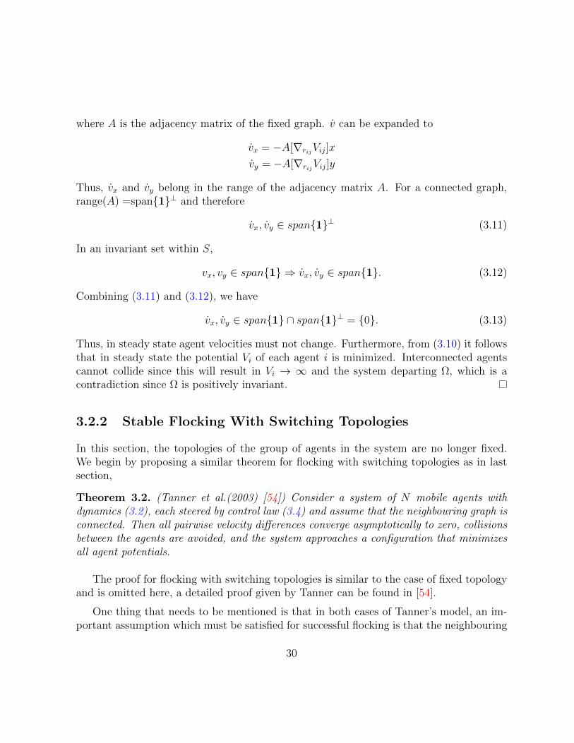
Figure 3.2: Fragmentation Phenomenon
graph G must remain connected. This guarantees that the network is always connectedin both cases. If this crucial assumption is not satisfied, one possible situation is thatthe initial positions of some agents are too far away from the rest, then the neighbour setof those agents are empty, which means they cannot interact with any other agents andleads to fragmentation of the flock. An example of fragmentation phenomenon is given inFig.3.2.
3.3 Flocking With Navigational Feeback
The model without navigational feedback can only lead to flocking for a very restrictedset of initial states, if the network connectivity assumption is not satisfied it may lead tofragmentation. In [45], Olfati-Saber introduced three kinds of agents based on Tanner’smodel: α− agents, β − agents and γ − agents. α− agent refer to a physical agent which
31
has the same meaning as previous model, while β−agent is introduced as a representationof all nearby obstacles whenever the α − agent is in close proximity of an obstacle , andγ−agent denotes a common group objective or virtual leader of the flock, which eliminatesthe fragmentation phenomenon. By applying these three new terms in the control inputs,Olfati-Saber’s algorithm has successfully led to flocking with obstacles avoidance ability.
One significant capability of Olfati-Saber’s algorithm is to allow a group of dynamicagents to maintain identical/quasi-identical inter-agent distances between interacting agents,i.e. group dynamics that satisfy the algebraic constrains in (3.2). We will present a dis-tributed algorithm for flocking in free-space, or free-flocking. (The flocking algorithm withobstacle avoidance capabilities is presented in section 3.5.) We refer to a physical agentwith equation of motion ri = ui as an α-agent. α-agents correspond to birds, or member ofa flock. An α-agent has a tendency to stay at a distance d > 0 from all of its neighbouringα-agents, this is the reason behind the name α-lattice. In free-flocking, each α-agent hasa control input that consists of three components:
ri = vi,
vi = ui, i = 1, . . . , N,(3.14)
ui = f gi + fdi + fγi (3.15)
where f gi = −∇riV (r) is a gradient-based term, fdi is a velocity consensus/alignment termthat acts as damping force, and fγi is a navigational feedback due to a group objective.Example of a group objective is a destination where a flock moves towards during migration.Olfati-Saber proposed an algorithm that can be used for creation of flocking motion in Rm
as follows:
ui = uαi + uγi , or
ui =∑j∈Ni
φα(‖rj − ri‖σ)nij +∑j∈Ni
aij(r)(vj − vi) + fγi (ri, vi) (3.16)
where nij is a vector along the line connecting ri to rj and is given by
nij =rj − ri√
1 + ε‖rj − ri‖2(3.17)
and φα is defined as in (2.8), [aij] is the adjacency matrix of the net G(r) and fγi is thenavigational feedback is given by:
fγi (ri, vi, rγ, vγ) = −c1(ri − rγ)− c2(vi − vγ), c1, c2 > 0. (3.18)
32
The pair (rγ, vγ) ∈ Rm×Rm is the state of a γ-agent. A γ-agent is a dynamic/static agentthat represents a group objective. Let (rd, vd) be a fixed pair of m-vectors that denote theinitial position and velocity of a γ-agent. A dynamic γ-agent has the following model
rγ = vγ
vγ = fγ(rγ, vγ)(3.19)
with (rγ(0), vγ(0)) = (rd, vd). A static γ-agent has a fixed state that is equal to (rd, vd) forall time. The design of fγ(rγ, vγ) for a dynamic γ-agent is part of tracking control designfor a group of agents. For example, the choice of fγ = 0 leads to a γ-agent that movesalong a straight line with a desired velocity vd.
3.3.1 Collective Dynamics
The collective dynamics of a group of α-agents applying protocol (3.16) is in the form:
collective dynamics :
r = v
v = −∇V (r)− L(r)v + fγ(r, v, rγ, vγ)(3.20)
where V (r) is a smooth collective potential function given in (2.6) and L(r) is the m-dimensional Laplacian of the net G(r) with a position-dependent adjacency matrix A(r) =[aij(r)], r, v are the state vector of ri, vi respectively.
The first expected result is that with fγ = 0, system (3.20) is a dissipative particlesystem with Hamiltonian:
H(r, v) = V (r) +N∑i=1
‖vi‖2 (3.21)
This is due to H = −vT L(r)v ≤ 0 and the fact that the multi-dimensional graph LaplacianL(r) is a positive semidefinite matrix for all r. The key in stability analysis of collective dy-namics is employing a correct coordinate system that allows the use of LaSalle’s invarianceprinciple. One naive approach is to use H(r, v) in the (r, v)-coordinates. The reason suchan approach does not work is that one cannot establish the boundedness of solutions. Dur-ing fragmentation, the solution cannot remain bounded. Therefore, Olfati-Saber proposedthe use of a moving frame to analyze the stability of flocking motion.
33
3.3.2 Decomposition Dynamics
Consider a moving frame that is centred at rc, the centre of mass of all agents. LetAve(z) = 1
n
∑ni=1 zi denote the average of the zi’s with z = col(z1, . . . , zn). Let rc = Ave(r)
and vc = Ave(v) denote the position and velocity of the origin of the moving frame. Thenrc(t) = vc(t) and vc(t) = Ave(u(t)). Our objective is to separate the analysis of the motionof the centre of the group with respect to the reference frame from the collective motion ofthe agents in the moving frame. The position and velocity of agent i in the moving frameare given by
ri = ri − rcvi = vi − vc
(3.22)
The relative position and velocities remain the same in the moving frame, i.e. rj−ri = rj−riand vj − vi = vj − vi. Thus, V (r) = V (r) and ∇V (r) = ∇V (r). The control input in themoving frame can be expressed as
uαi =∑j∈Ni
φα(‖rj − ri‖σ)nij +∑j∈Ni
aij(r)(vj − vi) (3.23)
with aij(r) = ph(‖rj − ri‖σ)/rα. Now we will present a decomposition lemma that is thebasis for posing a structural stability problem for “dynamic flocks” (a dynamic networkwith a topology that is a connected net and nodes that are particles).
Lemma 3.1. (Decomposition) (Olfati-Saber et al.(2004) [45]) Suppose that the naviga-tional feedback fγ(r, v) is linear, i.e. there exists a decomposition of fγ(r, v) of the followingform:
fγ(r, v, rγ, vγ) = g(r, v) + h(rc, vc, rγ, vγ). (3.24)
Then, the collective dynamics of a group of agents can be decomposed as n second-ordersystems in the moving frame:
structural dynamics :
˙r = v˙v = −∇V (r)− L(v) + g(r, v)
(3.25)
and one second-order system in the reference frame:
translational dynamics :
rc = vc
vc = h(rc, vc, rγ, vγ)(3.26)
34
where
g(r, v) =− c1r − c2v (3.27)
h(rc, vc, rγ, vγ) =− c1(rc − rγ)− c2(vc − vγ) (3.28)
and (rγ, vγ) is the state of γ-agent.
A detailed proof of this lemma is given by Olfati-Saber in [45].
3.3.3 Stability Analysis
According to the decomposition lemma, we are now at the position to define stable flockingmotion as the combination of the following forms of stability properties:
1. Stability of certain equilibria of the structural dynamics in the moving frame.
2. Stability of a desired equilibrium of the translational dynamics in the reference frame.
The challenging part of stability analysis for a flocking algorithm is to establish part 1.Analysis of part 2 is far more simple than part 1. As far as animal behaviour is concerned,the translational dynamics of a flock does not necessarily have to possess an equilibriumpoint that is stable or asymptotically stable. A flock of birds could circle an area overand over or move in a erratic and unpredictable manner. However, from an engineeringperspective, an overall control over the collective behaviour of a flock is highly desired. Infact, the reason to perform flocking for UAVs is to steer a group of vehicles from point Ato B as a whole. Thus, in robotics or engineering applications, performing the second taskbecomes very crucial. As a consequence, flocking protocols such as (3.16) that account forthe group objective are beneficial for engineering applications.
The significant differences between Tanner’s model and Olfati-Saber’s model are dueto the differences in their perspective structural dynamics. Given Tanner’s model whichhas no navigational feedback, one obtains the following structural dynamics:
Σ1 :
˙r = v˙v = −∇V (r)− L(r)v
(3.29)
with a positive semidefinite Laplacian matrix L(r). In comparison, the structural dynamicsof a group of agents with a γ-agent (navigational feedback) in Olfati-Saber’s model is inthe form:
35
Σ2 :
˙r = v˙v = −∇Uλ(r)−D(r)v
(3.30)
where Uλ is called the aggregate potential function and is defined by
Uλ(r) = V (r) + λJ(r). (3.31)
The map J(r) = 12
∑ni=1 ‖ri‖2 is the moment of inertia of all agents and λ = c1 > 0 is a
parameter of the navigational feedback, and the matrix D(r) = c2Im + L(r) is a positivedefinite matrix with c2 > 0.
Define the structural dynamics of system (3.29) and (3.30) as follows:
H(r, v) = V (r) +K(v) (3.32)
Hλ(r, v) = Uλ(r) +K(v) (3.33)
where K(v) = 12
∑ni ‖vi‖2 is the kinetic energy of the agents in the moving frame. We now
need to define “cohesion of a group” and “flocks”.
Definition 3.3. (a cohesive group) Let (r(t), v(t)) be the state trajectory of a group ofdynamic agents over the time interval [t0, tf ]. We say the group is cohesive for all t ∈ [t0, tf ]if there exists a ball of radius R > 0 centred at rc(t) = Ave(r(t)) that contains all the agentsfor all time t ∈ [t0, tf ], i.e. ∃R > 0 : ‖r‖ ≤ R, ∀t ∈ [t0, tf ].
Definition 3.4. (flocks, quasi-flocks, dynamic flocks) The configuration r of a set of pointsν is called a flock with interaction range R if the net G(r) is connected. r is called a quasi-flock if G(r) has a giant component (i.e. a connected subgraph with relatively large numberof nodes). A group of α-agents are called a dynamic flock over the time interval [t0, tf ) ifat every moment t ∈ [t0, tf ), they are a flock.
Theorem 3.3. (Olfati-Saber et al.(2004) [45]) Consider a group of α-agents with structuraldynamics Σ1 (3.29). Let ωc = (r, v)|H(r, v) ≤ c be a set of the Hamiltonian H(r, v) of(3.29) such that for any solution starting in ωc, the group of agents is cohesive for all t ≥ 0.Then, the follow statements hold:
1. Solution of the structural dynamics converges to an equilibrium (r∗, 0) with a config-uration r∗ that is an α-lattice.
2. The velocity of all agents asymptotically match in the reference frame.
36
3. Given c < c∗ = Ψα(0), no inter-agent collisions occur for all t ≤ 0.
Proof. Any solution (r(t), v(t)) of the collective dynamics of α-agents with structural dy-namics Σ1 is uniquely mapped to a solution (r(t), v(t)) of the structural dynamics. Wehave
H(r, v) = −vT L(r)v = −1
2
∑(i,j)∈ε(r)
aij(r)‖vj − vi‖2 ≤ 0 (3.34)
which means the structural energy H(r, v) is non-increasing for all t ≥ 0. In addition,H(r(t), v(t)) ≤ c for all t ≥ 0 implies Ωc is an invariant set. This guarantees that thevelocity mismatch is upper bounded by c because of
K(v(t)) ≤ H(r(t), v(t)) ≤ c, ∀t ≥ 0.
By assumption, for any solution starting in Ωc, the group is cohesive in all time t ≥0. Hence, there exists an R > 0 such that ‖r(t)‖ ≤ R, ∀t ≥ 0. The combination ofboundedness of velocity mismatch and group cohesion guarantees boundedness of solutionof Σ1 starting in Ωc. This fact is the result of the following inequality:
‖(r(t), v(t))‖2 = ‖r(t)‖2 + ‖v(t)‖2 ≤ R2 + 2c = C (3.35)
where C > 0 is a constant.
From LaSalle’s invariance principle, all the solutions of Σ1 starting in Ω1 converge tothe largest invariant set in E = (r, v) ∈ Ωc : H = 0. However since the group of α-agentsconstitutes a dynamic flock for all t ≥ 0, G(r(t)) is a connected graph for all t ≥ 0. Thus,based on equation (3.34), we know that the velocities of all agents match in the movingframe, i.e. v1 = · · · = vn. But
∑i vi = 0, therefor, vi = 0 for all i. This means that
the velocity of all agents asymptotically match in the reference frame, or v1 = · · · = vn,which proves part 2. Moreover, the configuration r asymptotically converges to a fixedconfiguration r∗ that is an extrema of V (x), which means ∇V (r∗) = 0.
Since any solution of the system starting at certain equilibria such as local maximaor saddle points remain in those equilibria for all time, not all solutions of the systemconverge to a local minima. However, anything but a local minima is an unstable equilibria.Thus, almost every solution of the system converges to an equilibrium (r∗, 0) where r∗ isa local minima of V (r). According to Theorem 3.4, every local minima of V (r) is an α-lattice. Therefore, r∗ is an α-lattice and asymptotically all inter-agent distances between
37
neighbouring α-agents become equal to d. This finishes the proof of parts 1 and 2. Weprove part 3 by contradiction. Assume there exists a time t = t1 > 0 so that two distinctagents k, l collide, or rk(t1) = rl(t1). for all t ≥ 0, we have
V (r(t)) =1
2
∑i
∑j 6=i
ψα(‖rj − ri‖σ)
= ψα(‖rk(t)− rl(t)‖σ) +1
2
∑i∈ν\k,l
∑j∈ν\i,k,l
ψα(‖rj − ri‖σ)
≥ ψα(‖rk(t)− rl(t)‖σ).
Hence, V (r(t1)) ≥ ψα(0) = c∗. But the velocity mismatch is a non-negative quantity andΩc is an invariant set of H. This yields:
V (r(t)) = H(r(t), v(t))−K(v(t)) ≤ H(r(t), v(t)) ≤ c ≤ c∗, ∀t ≥ 0
which is in contradiction with an earlier inequality V (r(t1)) ≥ c∗. Therefore, no two agentscollide at any time t ≥ 0.
Theorem 3.4. Every local minima of V (r) is an α-lattice and vice versa.
A detailed proof given by Olfati-Saber can be found in [45].
The following result provides a global stability analysis with structural dynamics Σ2
(3.30) that is useful for creation of flocking motion for generic sets of initial conditions. Incomparison to Theorem 3.3, no assumptions regarding group cohesion or connectivity ofthe net are made in the following theorem:
Theorem 3.5. (Olfati-Saber et al.(2004) [45]) Consider a group of α-agents with structuraldynamics Σ2 (3.30) and c1, c2 > 0. Assume that the initial kinetic function K(v(0)) andinertia J(r(0)) are finite. Then, the following statements hold:
1. The group of agents remain cohesive for all t ≥ 0.
2. Solution of Σ2 (3.30) asymptotically converges to an equilibrium (r∗λ, 0) where r∗λ is alocal minima of Uλ(r).
3. The velocity of all agents asymptotically match in the reference frame.
38
4. Assume the initial structural energy of the agents is less than (k+1)c∗ with c∗ = ψα(0)and k > 0. Then, at most k distinct pairs of α-agents could possibly collide (k = 0guarantees a collision-free motion).
Proof. First, note that the multi-agent system with structural dynamics Σ2 and Hamilto-nian Hλ(r, v) = Uλ(r) +K(v) is a strictly dissipative particle system in the moving framebecause it satisfies
Hλ(r, v) = −vT (c2Im + L(r))v = −c2(vT v)− vT L(r)v < 0, ∀v 6= 0. (3.36)
Hence, the structural energy H(r, v) is monotonically decreasing for all (r, v) and
Hλ(r(t), v(t)) ≤ H0 = Hλ(r(0), v(0)) <∞.
The finiteness of H0 = V (r(0)) +λJ(r(0)) +K(v(0)) follows from the assumption that thecollective potential, the inertia and the velocity mismatch are all initially finite. Thus forall t ≥ 0, we have
Uλ(r(t)) ≤ H0
K(v(t)) ≤ H0
But Uλ = V (r) + λ2rT r with λ > 0 and V (r) ≥ 0 for all r, therefore
rT (t)r(t) ≤ 2H0
λ, ∀t ≥ 0.
This guarantees the cohesion of the group of α-agents for all t ≥ 0 because the position ofall agents remains in a ball of radius R =
√2H0/λ centred at rc. This cohesion property
together with boundedness of velocity mismatch, or K(v(t)) ≤ H0, guarantees boundednessof solutions of the structural dynamics Σ2. To see this, let z = col(r, v), then
‖z(t)‖2 = rT (t)r(t) + vT (t)v(t) ≤ 2(1
λ+ 1)H0 = C(λ) <∞.
Part 2 follows from LaSalle’s invariance principle. Notice that Hλ(r, v) = 0 implies v = 0.Thus similar to the argument in the proof of Theorem 3.3, almost every solution of themulti-agent system asymptotically converges to an equilibrium point z∗λ = (r∗λ, 0) where r∗λis a local minima of the aggregate potential function Uλ(r).
39
Part 3 follows from the fact that v asymptotically vanishes. Thus, the velocities of allagents asymptotically match in the reference frame.
To prove part 4, suppose H0 < (k + 1)c∗ and there are more than k distinct pairs ofagents that collide at a given time t1 ≥ 0. Hence, there must be at least k + 1 distinctpairs of agents that collide at time t1. This implies the collective potential of the particlesystem at time t = t1 is at least (k + 1)ψα(0). However, we have
H0 = V (r(0)) + λJ(r(0)) +K(v(0)) ≥ V (r(0)) ≥ (k + 1)ψα(0).
This contradicts the assumption that H0 < (k+1)c∗. Hence, no more than k distinct pairsof agents can possibly collide at any time t ≥ 0. Finally, with k = 0, no two agents cancollide.
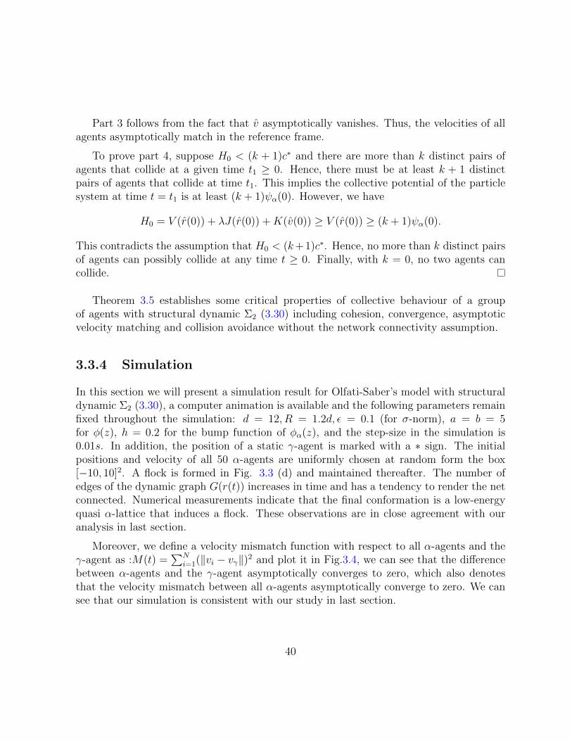
Theorem 3.5 establishes some critical properties of collective behaviour of a groupof agents with structural dynamic Σ2 (3.30) including cohesion, convergence, asymptoticvelocity matching and collision avoidance without the network connectivity assumption.
3.3.4 Simulation
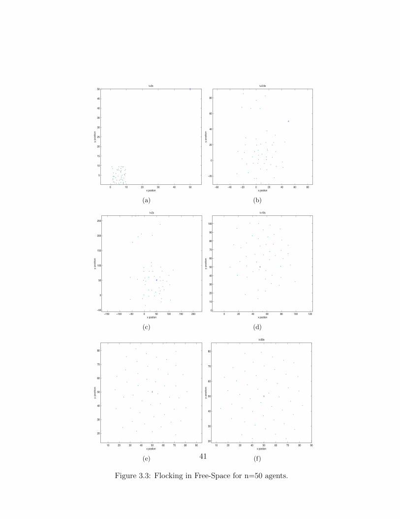
In this section we will present a simulation result for Olfati-Saber’s model with structuraldynamic Σ2 (3.30), a computer animation is available and the following parameters remainfixed throughout the simulation: d = 12, R = 1.2d, ε = 0.1 (for σ-norm), a = b = 5for φ(z), h = 0.2 for the bump function of φα(z), and the step-size in the simulation is0.01s. In addition, the position of a static γ-agent is marked with a ∗ sign. The initialpositions and velocity of all 50 α-agents are uniformly chosen at random form the box[−10, 10]2. A flock is formed in Fig. 3.3 (d) and maintained thereafter. The number ofedges of the dynamic graph G(r(t)) increases in time and has a tendency to render the netconnected. Numerical measurements indicate that the final conformation is a low-energyquasi α-lattice that induces a flock. These observations are in close agreement with ouranalysis in last section.
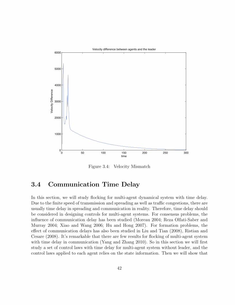
Moreover, we define a velocity mismatch function with respect to all α-agents and theγ-agent as :M(t) =
∑Ni=1(‖vi − vγ‖)2 and plot it in Fig.3.4, we can see that the difference
between α-agents and the γ-agent asymptotically converges to zero, which also denotesthat the velocity mismatch between all α-agents asymptotically converge to zero. We cansee that our simulation is consistent with our study in last section.
40
0 10 20 30 40 50
5
10
15
20
25
30
35
40
45
50
x postion
y p
ostion
t=0s
(a)
−60 −40 −20 0 20 40 60 80
−20
0
20
40
60
80
x postion
y p
ostion
t=0.6s
(b)
−150 −100 −50 0 50 100 150 200
−50
0
50
100
150
200
250
x postion
y p
ostion
t=2s
(c)
0 20 40 60 80 100 120
0
10
20
30
40
50
60
70
80
90
100
x postion
y p
ostion
t=10s
(d)
10 20 30 40 50 60 70 80 90
20
30
40
50
60
70
80
x postion
y p
ostio
n
(e)
10 20 30 40 50 60 70 80 90
20
30
40
50
60
70
80
x postion
y p
ostion
t=30s
(f)
Figure 3.3: Flocking in Free-Space for n=50 agents.
41
0 50 100 150 200 250 3000
1000
2000
3000
4000
5000
6000
time
Velocity difference between agents and the leaderV
elo
city D
iffe
ren
ce
Figure 3.4: Velocity Mismatch
3.4 Communication Time Delay
In this section, we will study flocking for multi-agent dynamical system with time delay.Due to the finite speed of transmission and spreading as well as traffic congestions, there areusually time delay in spreading and communication in reality. Therefore, time delay shouldbe considered in designing controls for multi-agent systems. For consensus problems, theinfluence of communication delay has been studied (Moreau 2004; Reza Olfati-Saber andMurray 2004; Xiao and Wang 2006; Hu and Hong 2007). For formation problems, theeffect of communication delays has also been studied in Liu and Tian (2008), Ristian andCesare (2008). It’s remarkable that there are few results for flocking of multi-agent systemwith time delay in communication (Yang and Zhang 2010). So in this section we will firststudy a set of control laws with time delay for multi-agent system without leader, and thecontrol laws applied to each agent relies on the state information. Then we will show that
42
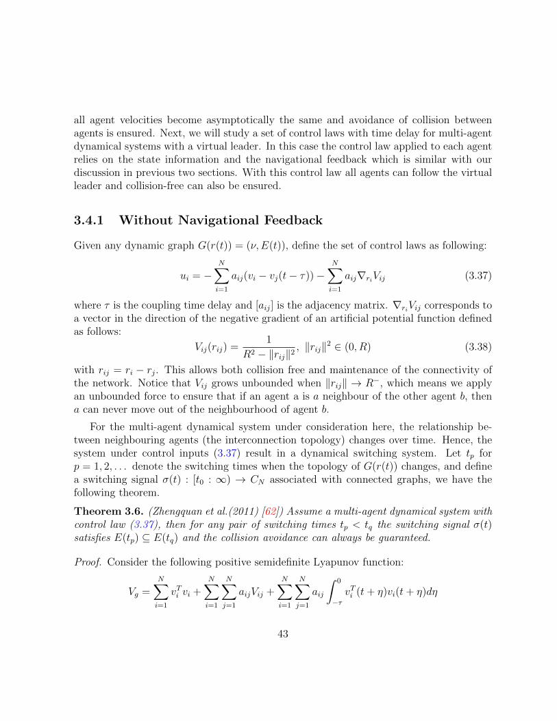
all agent velocities become asymptotically the same and avoidance of collision betweenagents is ensured. Next, we will study a set of control laws with time delay for multi-agentdynamical systems with a virtual leader. In this case the control law applied to each agentrelies on the state information and the navigational feedback which is similar with ourdiscussion in previous two sections. With this control law all agents can follow the virtualleader and collision-free can also be ensured.
3.4.1 Without Navigational Feedback
Given any dynamic graph G(r(t)) = (ν, E(t)), define the set of control laws as following:
ui = −N∑i=1
aij(vi − vj(t− τ))−N∑i=1
aij∇riVij (3.37)
where τ is the coupling time delay and [aij] is the adjacency matrix. ∇riVij corresponds toa vector in the direction of the negative gradient of an artificial potential function definedas follows:
Vij(rij) =1
R2 − ‖rij‖2, ‖rij‖2 ∈ (0, R) (3.38)
with rij = ri − rj. This allows both collision free and maintenance of the connectivity ofthe network. Notice that Vij grows unbounded when ‖rij‖ → R−, which means we applyan unbounded force to ensure that if an agent a is a neighbour of the other agent b, thena can never move out of the neighbourhood of agent b.
For the multi-agent dynamical system under consideration here, the relationship be-tween neighbouring agents (the interconnection topology) changes over time. Hence, thesystem under control inputs (3.37) result in a dynamical switching system. Let tp forp = 1, 2, . . . denote the switching times when the topology of G(r(t)) changes, and definea switching signal σ(t) : [t0 : ∞) → CN associated with connected graphs, we have thefollowing theorem.
Theorem 3.6. (Zhengquan et al.(2011) [62]) Assume a multi-agent dynamical system withcontrol law (3.37), then for any pair of switching times tp < tq the switching signal σ(t)satisfies E(tp) ⊆ E(tq) and the collision avoidance can always be guaranteed.
Proof. Consider the following positive semidefinite Lyapunov function:
Vg =N∑i=1
vTi vi +N∑i=1
N∑j=1
aijVij +N∑i=1
N∑j=1
aij
∫ 0
−τvTi (t+ η)vi(t+ η)dη
43
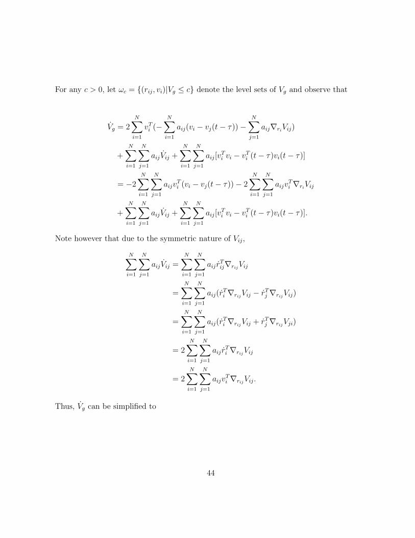
For any c > 0, let ωc = (rij, vi)|Vg ≤ c denote the level sets of Vg and observe that
Vg = 2N∑i=1
vTi (−N∑i=1
aij(vi − vj(t− τ))−N∑j=1
aij∇riVij)
+N∑i=1
N∑j=1
aijVij +N∑i=1
N∑j=1
aij[vTi vi − vTi (t− τ)vi(t− τ)]
= −2N∑i=1
N∑j=1
aijvTi (vi − vj(t− τ))− 2
N∑i=1
N∑j=1
aijvTi ∇riVij
+N∑i=1
N∑j=1
aijVij +N∑i=1
N∑j=1
aij[vTi vi − vTi (t− τ)vi(t− τ)].
Note however that due to the symmetric nature of Vij,
N∑i=1
N∑j=1
aijVij =N∑i=1
N∑j=1
aij rTij∇rijVij
=N∑i=1
N∑j=1
aij(rTi ∇rijVij − rTj ∇rijVij)
=N∑i=1
N∑j=1
aij(rTi ∇rijVij + rTj ∇rijVji)
= 2N∑i=1
N∑j=1
aij rTi ∇rijVij
= 2N∑i=1
N∑j=1
aijvTi ∇rijVij.
Thus, Vg can be simplified to
44
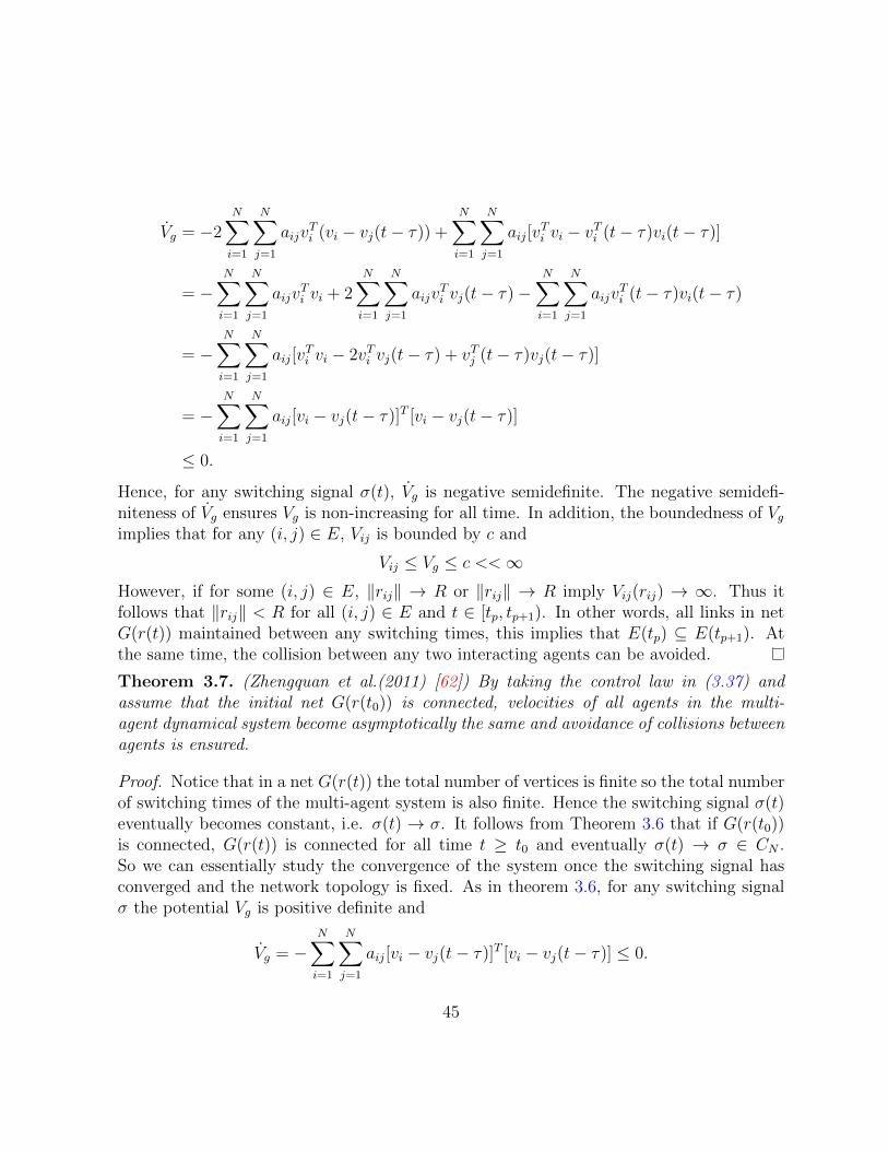
Vg = −2N∑i=1
N∑j=1
aijvTi (vi − vj(t− τ)) +
N∑i=1
N∑j=1
aij[vTi vi − vTi (t− τ)vi(t− τ)]
= −N∑i=1
N∑j=1
aijvTi vi + 2
N∑i=1
N∑j=1
aijvTi vj(t− τ)−
N∑i=1
N∑j=1
aijvTi (t− τ)vi(t− τ)
= −N∑i=1
N∑j=1
aij[vTi vi − 2vTi vj(t− τ) + vTj (t− τ)vj(t− τ)]
= −N∑i=1
N∑j=1
aij[vi − vj(t− τ)]T [vi − vj(t− τ)]
≤ 0.
Hence, for any switching signal σ(t), Vg is negative semidefinite. The negative semidefi-niteness of Vg ensures Vg is non-increasing for all time. In addition, the boundedness of Vgimplies that for any (i, j) ∈ E, Vij is bounded by c and
Vij ≤ Vg ≤ c <<∞However, if for some (i, j) ∈ E, ‖rij‖ → R or ‖rij‖ → R imply Vij(rij) → ∞. Thus itfollows that ‖rij‖ < R for all (i, j) ∈ E and t ∈ [tp, tp+1). In other words, all links in netG(r(t)) maintained between any switching times, this implies that E(tp) ⊆ E(tp+1). Atthe same time, the collision between any two interacting agents can be avoided.
Theorem 3.7. (Zhengquan et al.(2011) [62]) By taking the control law in (3.37) andassume that the initial net G(r(t0)) is connected, velocities of all agents in the multi-agent dynamical system become asymptotically the same and avoidance of collisions betweenagents is ensured.
Proof. Notice that in a net G(r(t)) the total number of vertices is finite so the total numberof switching times of the multi-agent system is also finite. Hence the switching signal σ(t)eventually becomes constant, i.e. σ(t) → σ. It follows from Theorem 3.6 that if G(r(t0))is connected, G(r(t)) is connected for all time t ≥ t0 and eventually σ(t) → σ ∈ CN .So we can essentially study the convergence of the system once the switching signal hasconverged and the network topology is fixed. As in theorem 3.6, for any switching signalσ the potential Vg is positive definite and
Vg = −N∑i=1
N∑j=1
aij[vi − vj(t− τ)]T [vi − vj(t− τ)] ≤ 0.
45
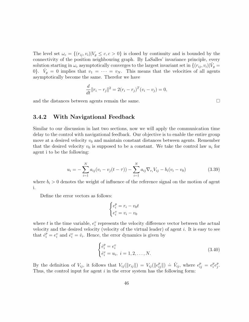
The level set ωc = (rij, vi)|Vg ≤ c, c > 0 is closed by continuity and is bounded by theconnectivity of the position neighbouring graph. By LaSalles’ invariance principle, everysolution starting in ωc asymptotically converges to the largest invariant set in (rij, vi)|Vg =0. Vg = 0 implies that v1 = · · · = vN . This means that the velocities of all agentsasymptotically become the same. Therefor we have
d
dt‖ri − rj‖2 = 2(ri − rj)T (vi − vj) = 0,
and the distances between agents remain the same.
3.4.2 With Navigational Feedback
Similar to our discussion in last two sections, now we will apply the communication timedelay to the control with navigational feedback. Our objective is to enable the entire groupmove at a desired velocity v0 and maintain constant distances between agents. Rememberthat the desired velocity v0 is supposed to be a constant. We take the control law ui foragent i to be the following:
ui = −N∑i=1
aij(vi − vj(t− τ))−N∑i=1
aij∇riVij − bi(vi − v0) (3.39)
where bi > 0 denotes the weight of influence of the reference signal on the motion of agenti.
Define the error vectors as follows:epi = ri − v0tevi = vi − v0
where t is the time variable, evi represents the velocity difference vector between the actualvelocity and the desired velocity (velocity of the virtual leader) of agent i. It is easy to seethat epi = evi and evi = vi. Hence, the error dynamics is given by
epi = evievi = ui, i = 1, 2, . . . , N.
(3.40)
By the definition of Vij, it follows that Vij(‖rij‖) = Vij(‖epij‖).= Vij, where epij = epi e
pj .
Thus, the control input for agent i in the error system has the following form:
46
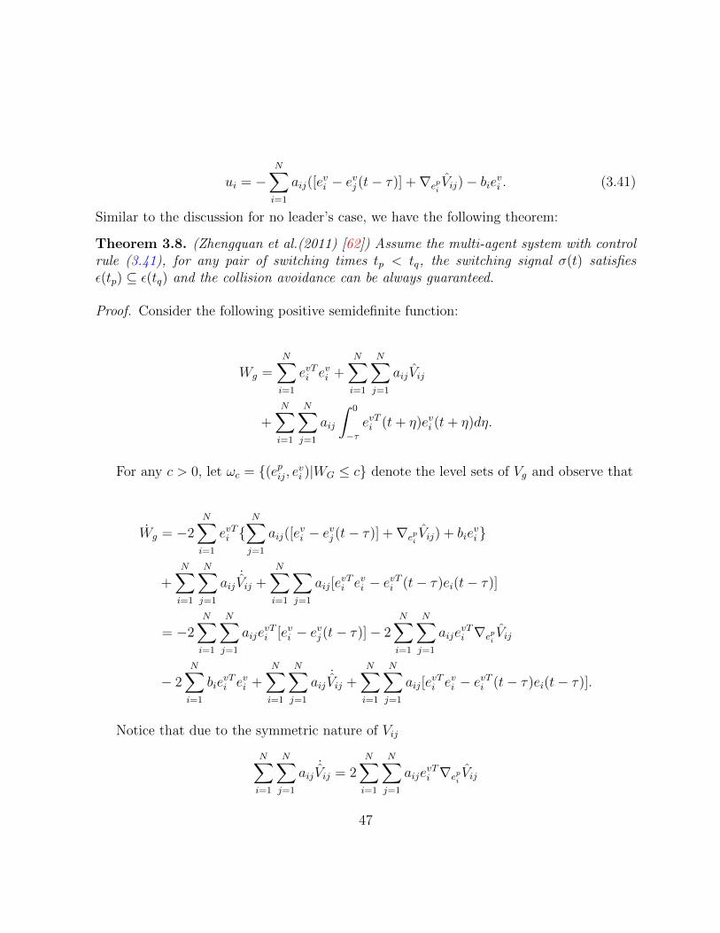
ui = −N∑i=1
aij([evi − evj (t− τ)] +∇epi
Vij)− bievi . (3.41)
Similar to the discussion for no leader’s case, we have the following theorem:
Theorem 3.8. (Zhengquan et al.(2011) [62]) Assume the multi-agent system with controlrule (3.41), for any pair of switching times tp < tq, the switching signal σ(t) satisfiesε(tp) ⊆ ε(tq) and the collision avoidance can be always guaranteed.
Proof. Consider the following positive semidefinite function:
Wg =N∑i=1
evTi evi +N∑i=1
N∑j=1
aijVij
+N∑i=1
N∑j=1
aij
∫ 0
−τevTi (t+ η)evi (t+ η)dη.
For any c > 0, let ωc = (epij, evi )|WG ≤ c denote the level sets of Vg and observe that
Wg = −2N∑i=1
evTi N∑j=1
aij([evi − evj (t− τ)] +∇epi
Vij) + bievi
+N∑i=1
N∑j=1
aij˙Vij +
N∑i=1
∑j=1
aij[evTi evi − evTi (t− τ)ei(t− τ)]
= −2N∑i=1
N∑j=1
aijevTi [evi − evj (t− τ)]− 2
N∑i=1
N∑j=1
aijevTi ∇epi
Vij
− 2N∑i=1
bievTi evi +
N∑i=1
N∑j=1
aij˙Vij +
N∑i=1
N∑j=1
aij[evTi evi − evTi (t− τ)ei(t− τ)].
Notice that due to the symmetric nature of Vij
N∑i=1
N∑j=1
aij˙Vij = 2
N∑i=1
N∑j=1
aijevTi ∇epi
Vij
47
Thus Wg can be simplified to
Wg = −2N∑i=1
N∑j=1
aijevTi [evi − evj (t− τ)]
+N∑i=1
N∑j=1
aij[evTi evi − evTi (t− τ)ei(t− τ)]− 2
N∑i=1
bievTi evi
= −N∑i=1
N∑j=1
aijevTi evi + 2
N∑i=1
N∑j=1
aijevTi evj (t− τ)
−N∑i=1
N∑j=1
aijevTi (t− τ)ei(t− τ)− 2
N∑i=1
bievTi evi
= −N∑i=1
N∑j=1
aij[evTi evi − 2evTi evj (t− τ) + evTj (t− τ)ej(t− τ)]− 2
N∑i=1
bievTi evi
= −N∑i=1
N∑j=1
aij[evi − evj (t− τ)]T [evi − evj (t− τ)]− 2
N∑i=1
bievTi evi
≤ 0
Hence, for any switching signal σ(t), Wg is negative semidefinite. The negative semidefi-niteness of Wg ensures Wg is non-increasing for all time. Moreover, the boundedness of Wg
implies that for any (i, j) ∈ E, Vij is bounded by c
Vij ≤ Wg ≤ c <<∞.
However, if for some (i, j) ∈ E, ‖rij‖ → R or ‖epij‖ → 0, then Vij(epij)→∞. Thus it follows
that ‖epij‖ < R for all (i, j) ∈ E and t ∈ [tp, tp+1). In other words, all links in G(r(t)) aremaintained between switching times, which implies that E(tp) ⊆ E(tp+1). At the sametime, the collision between any two interacting agents can be avoided.
Theorem 3.9. (Zhengquan et al.(2011) [62]) By taking the control law (3.41), assumethat the initial net G(r(t0)) is connected, velocities of all agents in the multi-agent systemapproach asymptotically the leader’s velocity and avoidance of collisions between agents isensured.
48

Proof. Notice that in a net G(r(t)) the total number of vertices is finite so the total numberof switching times of the multi-agent system is also finite. Hence the switching signal σ(t)eventually becomes constant, i.e. σ(t)→ σ. It follows from Theorem 3.8 that if G(r(t0)) isconnected, G(r(t)) is connected for all time t ≥ t0 and eventually σ(t) → σ ∈ CN . So wecan essentially study the convergence of the system once the switching signal has convergedand the network topology is fixed. As in theorem 3.8, for any switching signal σ(t) thepotential Wg is positive definite and
Wg = −N∑i=1
N∑j=1
aij[evi − evj (t− τ)]T [evi − evj (t− τ)]− 2
N∑i=1
bievTi evi
≤ 0.
The level set ωc = (epij, epi )|Wg ≤ c, c > 0 is closed by continuity and is bounded
by the connectivity of the position neighbouring graph. By LaSalle’s invariance princi-ple, every solution starting in ωc asymptotically converges to the largest invariant set in(epij, evi )|Wg = 0. Wg = 0 implies that ev1 = · · · = evN = 0. This occurs only whenv1 = · · · = vN = v0 for i = 1, 2, . . . , N . Thus all agents’ velocities in the error systemremain the same and all equal to zero in the steady-state. Moreover, we have
d
dt‖epi − e
pj‖2 = 2(epi − e
pj)T (evi − evj ) = 0,
which implies the distances between agents are invariant.
3.5 Obstacle Avoidance Ability
In this section, we will present a distributed flocking algorithm with multiple obstacle-avoidance capability. The main idea is to use agent-based representation of all nearbyobstacles by creating a new species of agents called β-agents [38]. A β-agent is a kinematicagent that is induced by an α-agent whenever the α-agent is in close proximity of anobstacle. In the following, we will define the notion of a β-agent and specify the interactionprotocol between an α-agent and a β-agent. Moreover, we restrict our study to obstaclesthat lie in a connected convex region of Rm with boundaries that are smooth manifolds.More explicitly we mainly focus on obstacles that are either spheres or infinite walls asshown in Fig.3.5. We can approach to obstacle avoidance by summarizing in the followingsteps:
49
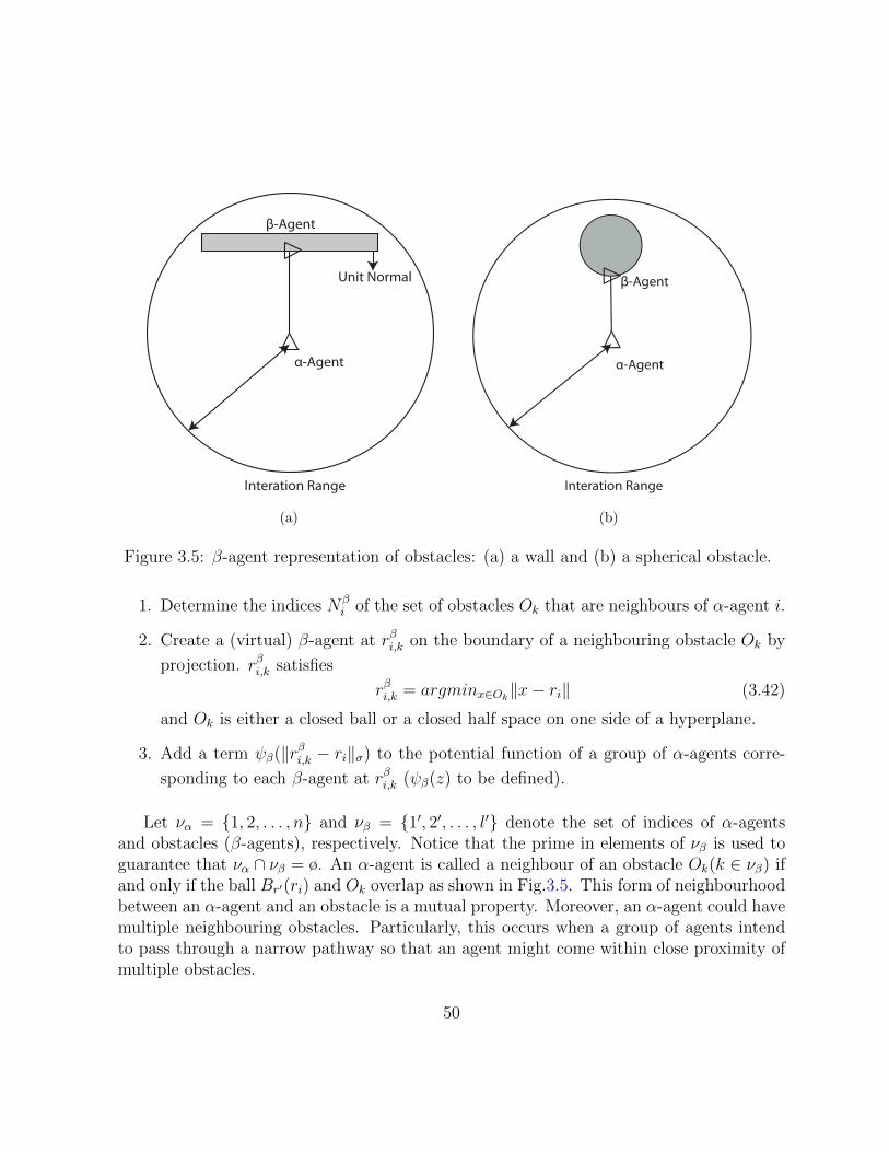
Unit Normal
Interation Range
β-Agent
α-Agent
(a)
α-Agent
Interation Range
β-Agent
(b)
Figure 3.5: β-agent representation of obstacles: (a) a wall and (b) a spherical obstacle.
1. Determine the indices Nβi of the set of obstacles Ok that are neighbours of α-agent i.
2. Create a (virtual) β-agent at rβi,k on the boundary of a neighbouring obstacle Ok by
projection. rβi,k satisfies
rβi,k = argminx∈Ok‖x− ri‖ (3.42)
and Ok is either a closed ball or a closed half space on one side of a hyperplane.
3. Add a term ψβ(‖rβi,k − ri‖σ) to the potential function of a group of α-agents corre-
sponding to each β-agent at rβi,k (ψβ(z) to be defined).
Let να = 1, 2, . . . , n and νβ = 1′, 2′, . . . , l′ denote the set of indices of α-agentsand obstacles (β-agents), respectively. Notice that the prime in elements of νβ is used toguarantee that να ∩ νβ = ø. An α-agent is called a neighbour of an obstacle Ok(k ∈ νβ) ifand only if the ball Br′(ri) and Ok overlap as shown in Fig.3.5. This form of neighbourhoodbetween an α-agent and an obstacle is a mutual property. Moreover, an α-agent could havemultiple neighbouring obstacles. Particularly, this occurs when a group of agents intendto pass through a narrow pathway so that an agent might come within close proximity ofmultiple obstacles.
50
We define the sets of α-neighbours and β-neighbours of an α-agent i ∈ να as follows:
Nαi = j ∈ να : ‖rj − ri‖ < R
Nβi = k ∈ νβ : ‖rβi,k − ri‖ < Rβ
where R,Rβ > 0 are interaction ranges of an α-agent with neighbouring α-agents andβ-agents, respectively. Here we choose Rβ < R.
The sets of α-neighbours and β-neighbours of an α-agent i ∈ να naturally define an(α, β)-net that is a spatially induced graph in the form
Gα,β(r) = Gα(r) +Gβ(r)
where Gα(r) = (να, εα(r)) is a net induced by configuration of all α-agents and Gβ(r) =(νβ, εβ(r)) is a directed bipartite graph induced by r and the set of obstacles O = Ok :k ∈ νβ where εβ(r) ⊆ να × νβ. The condition να ∩ νβ = ø guarantees well-posedness ofthe definition of the bipartite graph Gβ(r). More explicitly we have:
εα(r) = (i, j) : i ∈ να, j ∈ Nαi
εβ(r) = (i, k) : i ∈ να, k ∈ Nβi
and Gα,β(r) = (να ∪ νβ, εα(r) ∪ εβ(r)). Similarly, an (α, β)-frame net is a structure(Gα,β(r), r, r) where r denotes the configuration of all β-agents.
The new set of inter-agent and agent-to-obstacle algebraic constraints for an α-agent isspecifies as follows:
‖rj − ri‖ = d, ∀j ∈ Nαi
‖rβi,k − ri‖ = dβ, ∀k ∈ Nβi
(3.43)
A constrained α-lattice denoted by (r, O) consists of an α-lattice r and a set of obstacles Othat satisfy the set of constraints in (3.43). The relevant ratios of a constrained α-latticeare k = R/d and kβ = dβ/d = Rβ/R.
To achieve flocking in presence of obstacles, we use the following multi-species collectivepotential function for the multi-agent system:
V (r) = cα1Vα(r) + cβ1Vβ(r) + cγ1Vγ(r) (3.44)
51
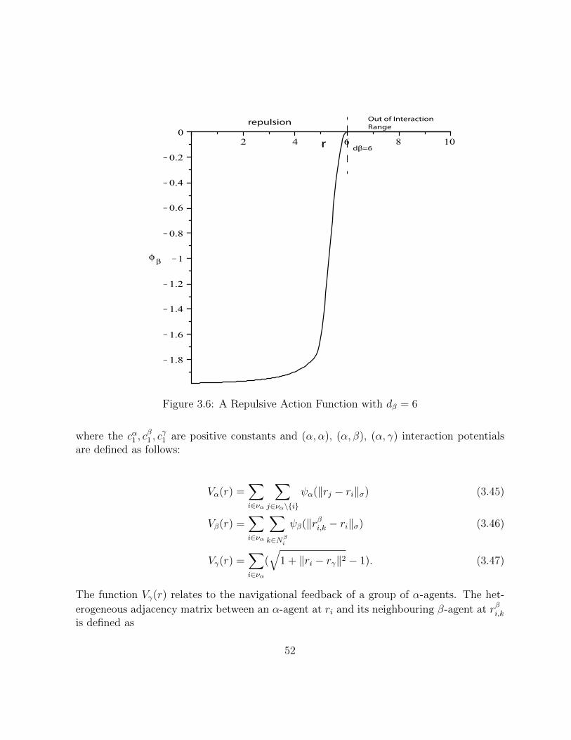
repulsion
dβ=6
Out of Interaction
Range
r
Figure 3.6: A Repulsive Action Function with dβ = 6
where the cα1 , cβ1 , c
γ1 are positive constants and (α, α), (α, β), (α, γ) interaction potentials
are defined as follows:
Vα(r) =∑i∈να
∑j∈να\i
ψα(‖rj − ri‖σ) (3.45)
Vβ(r) =∑i∈να
∑k∈Nβ
i
ψβ(‖rβi,k − ri‖σ) (3.46)
Vγ(r) =∑i∈να
(√
1 + ‖ri − rγ‖2 − 1). (3.47)
The function Vγ(r) relates to the navigational feedback of a group of α-agents. The het-
erogeneous adjacency matrix between an α-agent at ri and its neighbouring β-agent at rβi,kis defined as
52
bi,k(r) = ph(‖rβi,k − ri‖σ/dβ)
where dβ < Rβ with dβ = ‖dβ‖σ, Rβ = ‖Rβ‖σ. Define the repulsive action function asfollows:
φβ(z) = ρh(z/dβ)(σ1(z − dβ)− 1) (3.48)
with σ1(z) = z√1+z2
. Notice that φβ(z) vanishes smoothly to zero at z = dβ and remainszero for all z ≥ dβ as shown in Fig 3.6. Similarly define a repulsive pairwise potentialψβ(z) in the form
ψβ(z) =
∫ z
dβ
φβ(s)ds ≥ 0. (3.49)
From the point-of view of application, it is unreasonable to apply unbounded forcesto α-agents (vehicles/robots/animals). We avoid the use of repulsive potential functionswith unbounded derivatives such as 1/z or log(z) that are well-known examples of barrierfunctions. Clearly, −2 < ψ′β(z) ≤ 0 for all z ∈ R and thereby the derivative of ψβ(z) isuniformly bounded. Then we are ready to present the flocking algorithm with obstacle-avoidance capability:
We can divide the control input into three terms:
ui = uαi + uβi + uγi (3.50)
where uαi denotes the (α, α) interaction terms, uβi denotes the (α, β) interaction terms anduγi is a distributed navigational feedback. We explicitly specify each term as follows:
uαi =− cα1∇riVα(r) + cα2∑j∈Nα
i
aij(r)(vj − vi) (3.51)
=cα1∑j∈Nα
i
φα(‖rj − ri‖σ)nij + cα2∑j∈Nα
i
aij(vj − vi) (3.52)
uβi =− cβ1∇riVβ(r) + cβ2∑k∈Nβ
i
bi,k(r)(vβi,k − vi) (3.53)
=cβ1∑k∈Ni
φβ(‖rβi,k − ri‖σ)nβi,k + cβ2∑k∈Nβ
i
bi,k(r)(vβi,k − vi) (3.54)
uγi =− cγ1(ri − rγ)− cγ2(vi − vγ) (3.55)
53
where σ1(z) = z/√
1 + ‖z‖2 and cνη are positive constants for all η = 1, 2 and ν = α, β, γ.
The pair (rγ, vγ) is the state of a static/dynamic γ-agent. The vectors nij and nβi,k aregiven by
nij =rj − ri√
1 + ε‖rj − ri‖2
nβi,k =rβi,k − ri√
1 + ε‖rβi,k − ri‖2.
In terms of sensing requirements, we assume that every α-agent is equipped with rangesensors that allow the agent to measure the relative position between the closest point onan obstacle and itself. Both radars and laser radars can be used as range sensors, thereforethis assumption is feasible in practice. For the purpose of simulation of flocking motion,we use the projection of the position of an α-agent on the boundary of an obstacle.
Given an obstacle Ok and its neighbouring α-agent with state (ri, vi), the position andvelocity of a β-agent on a wall or a sphere is given by the following lemma:
Lemma 3.2. (Olfati-Saber et al.(2004) [45]) Let rβi,k, vβi,k with (i, k) ∈ να × νβ denote the
position and velocity of a β-agent generated by an α-agent with state (ri, vi) on an obstacleOk. Then
1. For an obstacle with a hyperplane boundary that has a unit normal ak and passesthrough the point yk, the position and velocity of the β-agent are determined by
rβi,k = Pri + (I − P )yk, vβi,k = Pvi
2. For a spherical obstacle with radius Rk centred at yk, the position and velocity of theβ-agent are given by
rβi,k = µri + (1− µ)yk, rβi,k = µPvi
where µ = Rk/‖ri − yk‖, ak = (ri − yk)/‖ri − yk‖, and P = I − akaTk
The following lemma demonstrates that the second term in uβi is in fact a valid dampingforce. This fact indicates that the overall particle system is dissipative.
54
Lemma 3.3. (Olfati-Saber et al.(2004) [45]) The force fβ between α-agents and β-agentswith elements fβi =
∑k∈Nβ
ibi,k(ri− rβi,k) is a valid damping force, i.e. Let Kr = 1
2
∑i ‖vi‖2
and suppose ri = fβi , the Kr ≤ 0.
Another question is whether the particle system obtained by applying control input(3.50) is dissipative. The answer in this case is not as predictable as the case of interactionsamong α-agents. The reason is that in free-flocking , every α-agent reciprocates the actionof its neighbouring α-agents, but in constrained flocking the (α, β)-net is a unidirectionalgraph.
Theorem 3.10. (Olfati-Saber et al.(2004) [45]) Consider a multi-agent system applyingcontrol input (3.50). Assume that the γ-agent is a static agent with a fixed state (rγ, vγ) =(rd, vd). Define the energy function H(r, v) = V (r) + T (r, v) with kinetic energy T (r, v) =12
∑Ni=1 ‖vi‖. Suppose there exists a finite time t0 ≥ 0 such that the average velocity of all
agents satisfies the following condition
n
2< vc(t), vd >≤ T (r(t), v(t)), ∀t ≥ t0. (3.56)
Then, the energy of the system is non-increasing (i.e. H(r(t), v(t)) ≤ 0) along the trajectoryof the collective dynamics of the multi-agent system for all t ≥ t0
Proof. By direct differentiation, we have
H(r, v) =< ∇Vα(r), v > + < ∇rVβ(r), v > + < ∇rβ , vβ > +
∑i∈να
< vi, uαi + uβi + uγi >
cβ1 < ∇rβVβ(r), vβ > +cα2∑
(i,j)∈εα(r)
aij(r) < vi, vj − vi >
+ cβ2∑i∈να
∑k∈Nβ
i
bi,k < vi, vβi,k − vi > −c
γ2
∑i∈να
< vi, vi − vd >
But
< ∇rβVβ(r), vβ > =∑i∈να
∑k∈Nβ
i
< ∇rβi,kVβ(r), vβi,k >
=∑i∈να
∑k∈Nβ
i
φβ(‖rj − ri‖σ) < nβi,k, vβi,k >
= 0
55
because vβi,k is tangent to the surface of the obstacle, whereas nβi,k is orthogonal to the
surface of the obstacle. Thus, H(r, v) satisfies
H(r, v) = −cα2 (vT L(r)v)+cβ2∑i∈να
∑k∈Nβ
i
bi,k < vi, vβi,k−vi > −2cγ2(T (r, v)−n
2(vTd vc)) ≤ 0, ∀t ≥ t0
where the second term in the last inequality is negative semidefinite based on Lemma. 3.3and the term T (r, v)− n
2(vTd vc) is by assumption non-negative for all t ≥ t0.
The interpretation of condition (3.56) for a group of particles with equal velocities isinteresting. In this case, vc = vi for all i, and therefore (3.56) reduces to the inequalityvTc vd ≤ ‖vc‖2. Let θc,d denote the misalignment angle between vectors vc and vd in Rm, i.e.cos(θc,d) =< vc, vd > /(‖vc‖‖vd‖). Suppose vc, vd 6= 0, then the group has to by sufficientlyagile, or ‖vc‖ ≥ v0 = ‖vd‖cos(θc,d). Intuitively, this can be interpreted as a collective effortby the group to keep up with the desired velocity vd. For a γ-agent with vd = 0, condition(3.56) trivially holds.
3.5.1 Simulation
In Fig.3.7 we present a simulation result for a multi-agent system with input control (3.50),a computer animation is available and the following parameters remain fixed throughoutthe simulation: d = 12, R = 1.2d, ε = 0.1 (for σ-norm), a = b = 5 for φ(z), h = 0.2 forthe bump function of φα(z) and h = 0.8 for φβ(z), and the step-size in the simulation is0.01s. In addition, the position of a static γ-agent is marked with a o sign, a sphericalobstacle which centred at (50, 50) with radius R = 20 is denoted by a red circle. Theinitial positions and velocity of all 15 α-agents are uniformly chosen at random form thebox [−20, 20]2. One can observe that the agents avoid collision with both other agents andthe spherical obstacle as moving forward, finally form an α-lattice shape around the γ-agent (navigational feedback). This has been numerically verified for the entire trajectoryof the agents and it is consistent with our analysis.
56
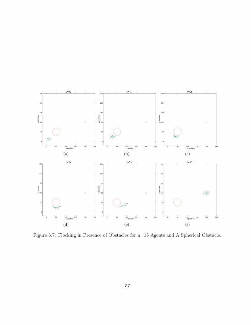
0 50 100 150 200 250
0
50
100
150
200
250
x position
y p
osi
tio
n
t=0s
(a)
0 50 100 150 200 250
0
50
100
150
200
250
y p
osi
tio
n
x position
t=1s
(b)
0 50 100 150 200 250
0
50
100
150
200
250
y p
osi
tio
n
x position
t=2s
(c)
0 50 100 150 200 250
0
50
100
150
200
250
y p
osi
tio
n
x position
t=3s
(d)
0 50 100 150 200 250
0
50
100
150
200
250
y p
osi
tio
n
x position
t=5s
(e)
0 50 100 150 200 250
0
50
100
150
200
250
x position
y p
osi
tio
n
t=15s
(f)
Figure 3.7: Flocking in Presence of Obstacles for n=15 Agents and A Spherical Obstacle.
57
Chapter 4
Flocking via Impulsive Control
In comparison with continuous control which had been studied in last two chapters, therehas been little work done on the design of impulsive control for multi-agent systems withswitching topologies. Impulsive control has some advantages compared with continuouscontrol, e.g., it is more flexible and energy-efficient than continuous control. Moreover, ithas been proved that impulsive control approach is effective and robust in synchronizationof chaotic systems and complex networks [63], and the controllers used in impulsive methodusually have relatively simple structure. The advantage of applying impulsive control ina self-driven, communicating multi-agent systems is to reduce energy and communicationcost. We can imagine that a bird in a flock is not flapping its wings all the time. Inspired bythis idea, we will propose a model which consists of both continuous and impulsive controlsin this chapter. For the continuous part, we will apply a smooth potential function whichguarantees cohesive and collision-free capabilities of agents in the system. Additionally, weapply impulsive controls to the system for the velocity alignment and consensus with thevirtual leader (navigational feedback).
4.1 Impulsive Consensus Problem
In this section we will start with studying the consensus problem for the multi-agentdynamical system. It can be described as multi-agent systems to develop distributedcontrol rules based on local information that enable all agents to reach a global agreementon certain interest [44], which can be understood as a special case of flocking problem formulti-agent dynamical systems.
58
We will consider the system with switching interconnection topologies in the prob-lem. Suppose that there is an infinite sequence of bounded, non-overlapping, contiguoustime-intervals [ti−1, ti), i = 1, 2, . . . , starting at t0 = 0. As we introduced in last chapter,G = G1, G2, . . . , Gn is a set of the graphs with all possible topologies, which includes allpossible interconnection graphs including n agents and a leader. Denote P = 1, 2, . . . , nas its index set. To describe the variable interconnection topology, we define a switchingsignal σ : [0,+∞) → P , which is piecewise-constant. Therefore, Ni(t), aij(t) are all timevarying, i = 1, 2, . . . , n, j = 1, 2, . . . , n. Moreover, in each time interval, Lp, p ∈ P associ-ated with the switching interconnection topology is also switching. However, in each timeinterval, Lp are time-invariant for some p ∈ P .
In this section, all the considered agents share a common state space Rm, which isri = (r1i , r
2i , . . . , r
mi )T and vi = (v1i , v
2i , . . . , v
mi )T . The leader of the multi-agent dynamical
system is assumed to be dynamic. Its underlying dynamics can be expressed as follows:r0 = v0
v0 = a(t) = a0(t) + δ(t)(4.1)
where a(t) is the input (accelaration). We assume that a0(t) is known and δ(t) is unknownbut bounded by a given upper bound L, i.e. ‖δ(t)‖ ≤ L.
The dynamics of each agent are described as follows:ri = vi + urivi = a0(t) + uvi
(4.2)
where uri , uvi ∈ Rm, i = 1, 2, . . . , n are control inputs.
Our object is to design appropriate control inputs of follower agents to track the leader.Applying impulsive control to (4.1), we have the following consensus algorithm for themulti-agent system,
59
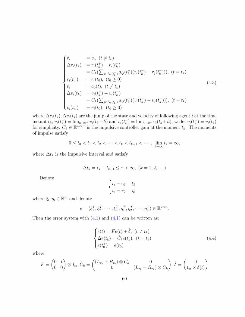
ri = vi, (t 6= tk)
∆ri(tk) = ri(t+k )− ri(t−k )
= Ck(∑
j∈Ni(t−k ) aij(t−k )(ri(t
−k )− rj(t−k ))), (t = tk)
ri(t+0 ) = ri(t0), (t0 ≥ 0)
vi = a0(t), (t 6= tk)
∆vi(tk) = vi(t+k )− vi(t−k )
= Ck(∑
j∈Ni(t−k ) aij(t−k )(vi(t
−k )− vj(t−k ))), (t = tk)
vi(t+0 ) = vi(t0), (t0 ≥ 0)
(4.3)
where ∆ri(tk),∆vi(tk) are the jump of the state and velocity of following agent i at the timeinstant tk, vi(t
+k ) = limh→0+ vi(tk+h) and vi(t
−k ) = limh→0− vi(tk+h), we let vi(t
−k ) = vi(tk)
for simplicity. Ck ∈ Rm×m is the impulsive controller gain at the moment tk. The momentsof impulse satisfy
0 ≤ t0 < t1 < t2 < · · · < tk < tk+1 < · · · , limk→∞
tk =∞,
where ∆tk is the impulsive interval and satisfy
∆tk = tk − tk−1 ≤ τ <∞, (k = 1, 2, . . . )
Denote ri − r0 = ξi
vi − v0 = ηi
where ξi, ηi ∈ Rm and denote
e = (ξT1 , ξT2 , · · · , ξTn , ηT1 , ηT2 , · · · , ηTn ) ∈ R2mn.
Then the error system with (4.1) and (4.1) can be written as:e(t) = Fe(t) + δ, (t 6= tk)
∆e(tk) = Cke(tk), (t = tk)
e(t+0 ) = e(t0)
(4.4)
where
F =
(0 I0 0
)⊗ Im, Ck =
((Lτk +Bτk)⊗ Ck 0
0 (Lτk +Bτk)⊗ Ck
), δ =
(0
1n × δ(t)
)60
and ∆e = (∆ξT1 , . . . ,∆ξTn ,∆η
T1 , . . . ,∆η
Tn )T , 1n = (1, 1, . . . , 1) ∈ Rm and ⊗ denotes the
Kronecker product. Lτk and Bτk are associated with the switching interconnection graphat time tk.
Lemma 4.1. Suppose that the directed graph G has a directed spanning tree and the rootof such tree has access to the leader. Then, all the eigenvalues of the matrix L + B havepositive real parts.
Now we are ready to provide the analysis of the impulsive consensus problem for multi-agent system with fixed and switching topologies. Firstly, we consider the graph with fixedtopology. Let βk be the maximum eigenvalue of matrix (I + Ck)
T (I + Ck), where Ck isassociated with the impulsive moment tk.
Theorem 4.1. (Qing et al.(2012) [44]) Assume that the interconnection graph among theagents is fixed and the graph G has a directed spanning tree. If βk and ∆tk satisfy thecondition that there exists ξ > 1 such that
η(tk − tk−1) + ln(ξ · βk) < 0
then the impulsive controlled multi-agent system (4.4) is asymptotically stable at origin.
Proof. Choose the candidate Lyapunov functional as
V (e(t)) = (e(t))T e(t)
For any t ∈ (tk−1, tk], the right and upper Dini’s derivative of V (e(t)) along the trajectoryof (4.4) is
D+V (e(t)) = (e(t))T e(t) + (e(t))T e(t)
= (e(t))T (F + F T )e(t) + 2δe(t)
= (e(t))T (F + F T )e(t) + 2L‖e(t)‖≤ (1 + 2L)V (e(t)) = ηV (e(t))
For L > 0, we have η > 1. Moreover, for any t ∈ (tk−1, tk],
V (e(t)) ≤ V (e(t+k−1))expη(t− tk−1) (4.5)
On the other hand, it follows from the second equation of system 4.4 that
V (e(t+k )) = e(tk)T e(tk)
= (e(tk))T (I + Cτk)
T (I + Cτk)e(tk)
≤ βkV (e(tk)), (k = 1, 2, . . . )
(4.6)
61
Let k = 1 in inequality (4.5), we have
V (e(t)) ≤ V (e(t0))expη(t− t0), t ∈ (t0, t1],
which lead toV (e(t1)) ≤ V (e(t0))expη(t1 − t0)
Let k = 1 in inequality (4.6), we have
V (e(t+1 )) ≤ β1V (e(t1)) ≤ β1V (e(t0))expη(t1 − t0)
Therefore, for t ∈ (t1, t2],
V (e(t)) ≤ V (e(t+1 ))expη(t− t1) ≤ β1V (e(t0))expη(t− t0),V (e(t2)) ≤ β1V (e(t0))expη(t2 − t0)V (e(t+2 )) ≤ β2V (e(t2)) ≤ β1β2V (e(t0))expη(t2 − t0)
Generally for t ∈ (tk, tk+1],
V (e(t)) ≤ β1 · · · βkV (e(t0))exp(η(t− t0))
From the condition η(tk − tk−1) + ln(ξ · βk) < 0, we have
βk · exp(η(tk − tk−1)) <1
ξ, (k = 1, 2, . . . ).
So we have
V (e(t)) ≤ β1 · · · βkV (e(t0)) · exp(η(t− tk)) · exp(η(tk − t0))
≤ 1
ξkV (e(t0)) · exp(η(t− tk)), t ∈ (tk, tk+1].
(4.7)
Notice that η > 0, ‖t− tk‖ is a finite constant, 1ξk→ 0 when k → ∞, hence, the origin is
globally asymptotically stable.
When the interconnection graph is switching, let βτk be the maximum eigenvalue of
matrix (I + Cτk)T (I + Cτk), where Cτk is associated with the impulsive gain Ck and ma-
trix Lτk + Bτk . Because there are finite possible interconnection graphs, we can takeβk =maxβτk : τk ∈ P. Following the similar proof of theorem 4.1, we can get thetheorem below.
62
Theorem 4.2. (Qing et al.(2012) [44]) Assume that the interconnection graph among theagents is switching and the graphs G1, G2, . . . , Gn all have directed spanning tree. If βk and∆tk satisfy the same condition as in theorem 4.1, then the impulsive controlled multi-agentsystem (4.4) is asymptotically stable at origin.
Remark 1. If ξ = 1, 4.7 can be written as
V (e(t)) ≤ V (e(t0)) · exp(η(t− tk))≤ V (e(t0))e
τ ·η
where τ is the maximum impulsive interval. So V (e(t)) < A as k → ∞, where A is aconstant. That is to say, the origin is stable but not asymptotically stable.
Remark 2. When the graphs G1, G2, . . . , Gn have spanning trees, from Lemma.4.1, alleigenvalues of matrix Lτk+Bτk have positive real part. Choose Ck = diagc1k, c2k, . . . , cmk , cik ∈(−1, 0), then the eigenvalues of matrix Ck have negative real part. By this means, the con-dition in theorem 4.1 will be satisfied.
4.2 Impulsive Flocking Problem
In last section we have studied the impulsive consensus problem for multi-agent systemand proven that with the impulsive controller under certain conditions, the error betweenthe following agents and the leader will asymptotically converged to zero. Notice thatthis kind of impulsive control will result in a jump of both the state and velocity of allfollower agents. For the flocking problem for multi-agent dynamical systems, it is notreasonable or applicable to apply a jump of the state of the agents from both engineeringand biological perspectives. Hence, what we can do is to apply such impulsive controlto only the velocities of agents in the systems as velocity pulses, which may be causedby a suddenly acceleration by a high-pressure jet engine of an unmanned vehicle from anengineering perspective, or a bird flapping its wings during a long-distant migration froman biological perspective.
Inspired by these ideas, in this section we will propose a hybrid system model, in whichwe apply continuous controls to the states of agents in the multi-agent dynamical systemin order to regulate the formation of the flock. Moreover, we apply impulsive controls tothe velocities of agents to achieve velocity alignment and consensus of all agents with thevirtual leader (navigational feedback). For the continuous control part, we will generatea smooth potential function and use the negative gradient of this potential function as
63
the acceleration inputs, which is similar with our discussion in Chapter 3, while at everymoment tk we apply a impulsive control to the velocity which is similar with our discussionin the impulsive consensus problem.
4.2.1 Without Damping
In this section, we will propose a hybrid system model without damping, the dynamics ofall agents in the multi-agent dynamical system can be described as follows,
ri = vi
vi = −∇riV (r)− c1(ri − r0) t 6= tk
∆vi(tk) = c2(vi(t−k )− v0(t−k )) t = tk
(4.8)
where ∆vi(tk) is the jump of the velocity of agent i at the time instant tk, for simplicitywe let vi(t
+k ) = vi(tk), c2 ∈ Rm×m is the impulsive controller gain at the moment tk. The
moments of impulse satisfy
0 ≤ t0 < t1 < t2 < · · · < tk < tk+1 < · · · , limk→∞
tk =∞,
where ∆tk is the impulsive interval and satisfy
∆tk = tk − tk−1 ≤ τ <∞, (k = 1, 2, . . . )
For the potential function V (r) we will use the same definition as in (2.6).
As our discussion for continuous control in Chapter 3, we can analyze stability bystudying the collective dynamics of the model, firstly we can write the collective dynamicsof system (4.8) in the following form:
r = v
v = −∇V (r) + f1(r, r0) t 6= tk
∆v = f2(v(t−k ), v0(t−k )) t = tk
(4.9)
where f1(r, r0) and f2(v, v0) are position and velocity feedback given by the virtual leaderrespectively.
Our objective is to separate the analysis of the motion of the centre of the group withrespect to the reference frame from the collective motion of the particles in the moving
64
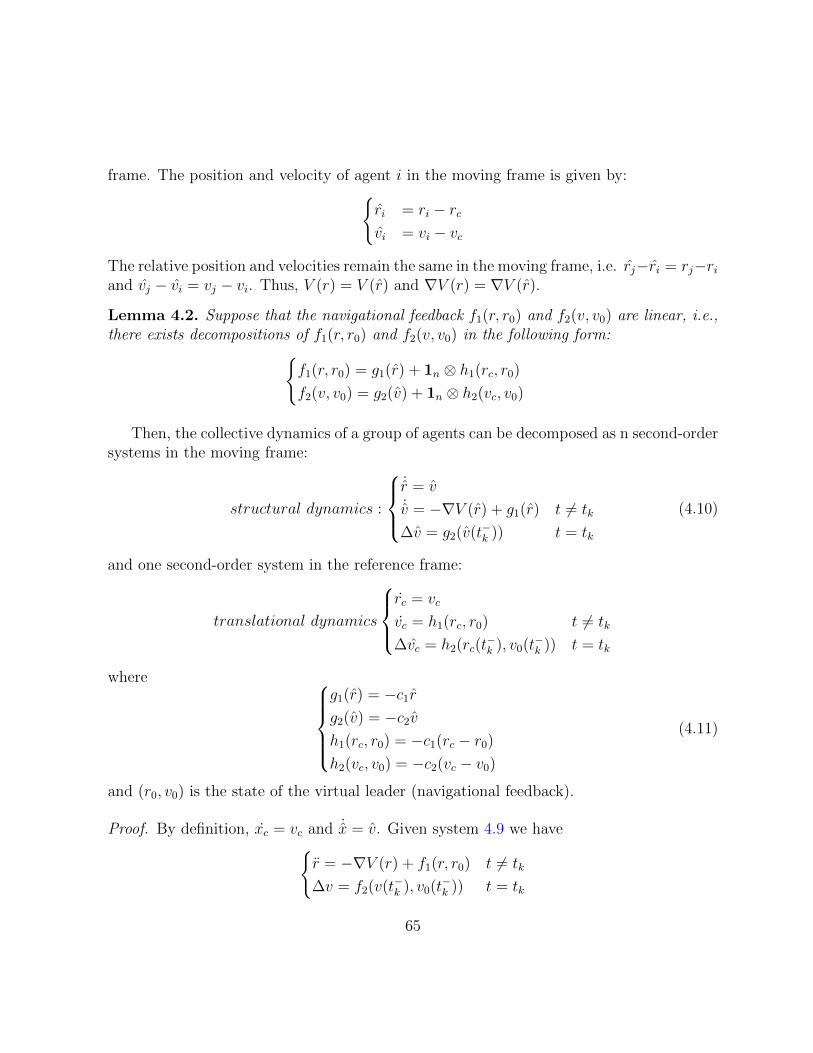
frame. The position and velocity of agent i in the moving frame is given by:ri = ri − rcvi = vi − vc
The relative position and velocities remain the same in the moving frame, i.e. rj−ri = rj−riand vj − vi = vj − vi. Thus, V (r) = V (r) and ∇V (r) = ∇V (r).
Lemma 4.2. Suppose that the navigational feedback f1(r, r0) and f2(v, v0) are linear, i.e.,there exists decompositions of f1(r, r0) and f2(v, v0) in the following form:
f1(r, r0) = g1(r) + 1n ⊗ h1(rc, r0)f2(v, v0) = g2(v) + 1n ⊗ h2(vc, v0)
Then, the collective dynamics of a group of agents can be decomposed as n second-ordersystems in the moving frame:
structural dynamics :
˙r = v˙v = −∇V (r) + g1(r) t 6= tk
∆v = g2(v(t−k )) t = tk
(4.10)
and one second-order system in the reference frame:
translational dynamics
rc = vc
vc = h1(rc, r0) t 6= tk
∆vc = h2(rc(t−k ), v0(t
−k )) t = tk
where g1(r) = −c1rg2(v) = −c2vh1(rc, r0) = −c1(rc − r0)h2(vc, v0) = −c2(vc − v0)
(4.11)
and (r0, v0) is the state of the virtual leader (navigational feedback).
Proof. By definition, xc = vc and ˙x = v. Given system 4.9 we haver = −∇V (r) + f1(r, r0) t 6= tk
∆v = f2(v(t−k ), v0(t−k )) t = tk
65
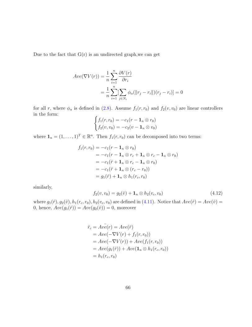
Due to the fact that G(r) is an undirected graph,we can get
Ave(∇V (r)) =1
n
n∑i=1
∂V (r)
∂ri
=1
n
n∑i=1
[∑j∈Ni
φα(‖rj − ri‖)(rj − ri)] = 0
for all r, where φα is defined in (2.8). Assume f1(r, r0) and f2(v, v0) are linear controllersin the form:
f1(r, r0) = −c1(r − 1n ⊗ r0)f2(v, v0) = −c2(v − 1n ⊗ v0)
where 1n = (1, . . . , 1)T ∈ Rn. Then f1(r, r0) can be decomposed into two terms:
f1(r, r0) = −c1(r − 1n ⊗ r0)= −c1(r − 1n ⊗ rc + 1n ⊗ rc − 1n ⊗ r0)= −c1(r + 1n ⊗ rc − 1n ⊗ r0)= −c1(r + 1n ⊗ (rc − r0))= g1(r) + 1n ⊗ h1(rc, r0)
similarly,f2(v, v0) = g2(v) + 1n ⊗ h2(vc, v0) (4.12)
where g1(r), g2(v), h1(rc, r0), h2(vc, v0) are defined in (4.11). Notice that Ave(r) = Ave(v) =0, hence, Ave(g1(r)) = Ave(g2(v)) = 0, moreover
rc = ¨Ave(r) = Ave(r)
= Ave(−∇V (r) + f1(r, r0))
= Ave(−∇V (r)) + Ave(f1(r, r0))
= Ave(g1(r)) + Ave(1n ⊗ h1(rc, r0))= h1(rc, r0)
66
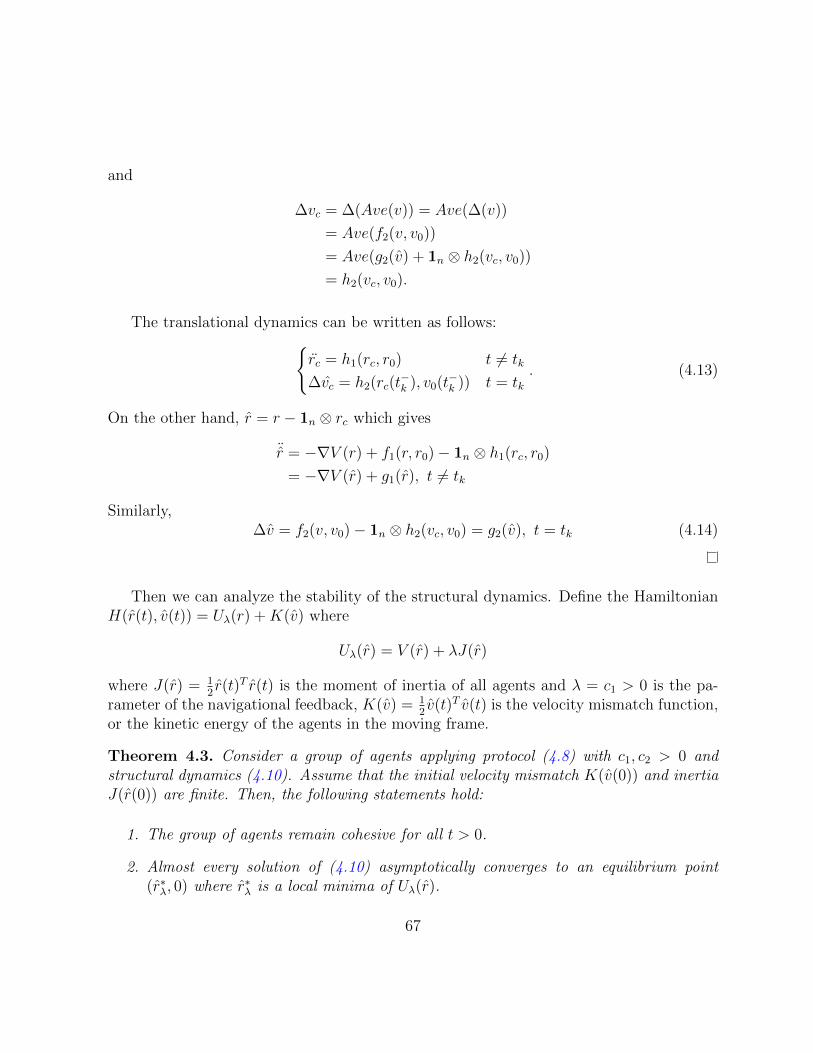
and
∆vc = ∆(Ave(v)) = Ave(∆(v))
= Ave(f2(v, v0))
= Ave(g2(v) + 1n ⊗ h2(vc, v0))= h2(vc, v0).
The translational dynamics can be written as follows:rc = h1(rc, r0) t 6= tk
∆vc = h2(rc(t−k ), v0(t
−k )) t = tk
. (4.13)
On the other hand, r = r − 1n ⊗ rc which gives
¨r = −∇V (r) + f1(r, r0)− 1n ⊗ h1(rc, r0)= −∇V (r) + g1(r), t 6= tk
Similarly,∆v = f2(v, v0)− 1n ⊗ h2(vc, v0) = g2(v), t = tk (4.14)
Then we can analyze the stability of the structural dynamics. Define the HamiltonianH(r(t), v(t)) = Uλ(r) +K(v) where
Uλ(r) = V (r) + λJ(r)
where J(r) = 12r(t)T r(t) is the moment of inertia of all agents and λ = c1 > 0 is the pa-
rameter of the navigational feedback, K(v) = 12v(t)T v(t) is the velocity mismatch function,
or the kinetic energy of the agents in the moving frame.
Theorem 4.3. Consider a group of agents applying protocol (4.8) with c1, c2 > 0 andstructural dynamics (4.10). Assume that the initial velocity mismatch K(v(0)) and inertiaJ(r(0)) are finite. Then, the following statements hold:
1. The group of agents remain cohesive for all t > 0.
2. Almost every solution of (4.10) asymptotically converges to an equilibrium point(r∗λ, 0) where r∗λ is a local minima of Uλ(r).
67
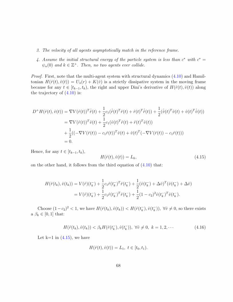
3. The velocity of all agents asymptotically match in the reference frame.
4. Assume the initial structural energy of the particle system is less than c∗ with c∗ =ψα(0) and k ∈ Z+. Then, no two agents ever collide.
Proof. First, note that the multi-agent system with structural dynamics (4.10) and Hamil-tonian H(r(t), v(t)) = Uλ(r) + K(v) is a strictly dissipative system in the moving framebecause for any t ∈ [tk−1, tk), the right and upper Dini’s derivative of H(r(t), v(t)) alongthe trajectory of (4.10) is:
D+H(r(t), v(t)) = ∇V (r(t))T ˙r(t) +1
2c1( ˙r(t)T r(t) + r(t)T ˙r(t)) +
1
2( ˙v(t)T v(t) + v(t)T ˙v(t))
= ∇V (r(t))T v(t) +1
2c1(v(t)T r(t) + r(t)T v(t))
+1
2((−∇V (r(t))− c1r(t))T v(t) + v(t)T (−∇V (r(t))− c1r(t)))
= 0.
Hence, for any t ∈ [tk−1, tk),H(r(t), v(t)) = Lk, (4.15)
on the other hand, it follows from the third equation of (4.10) that:
H(r(tk), v(tk)) = V (r)(t−k ) +1
2c1r(t
−k )T r(t−k ) +
1
2(v(t−k ) + ∆v)T (v(t−k ) + ∆v)
= V (r)(t−k ) +1
2c1r(t
−k )T r(t−k ) +
1
2(1− c2)2v(t−k )T v(t−k ).
Choose (1− c2)2 < 1, we have H(r(tk), v(tk)) < H(r(t−k ), v(t−k )), ∀v 6= 0, so there existsa βk ∈ [0, 1] that:
H(r(tk), v(tk)) < βkH(r(t−k ), v(t−k )), ∀v 6= 0, k = 1, 2, · · · (4.16)
Let k=1 in (4.15), we have
H(r(t), v(t)) = L1, t ∈ [t0, t1).
68
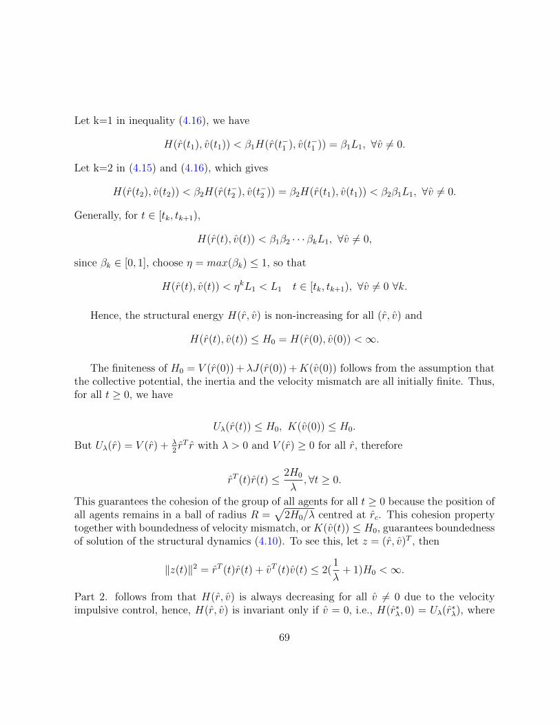
Let k=1 in inequality (4.16), we have
H(r(t1), v(t1)) < β1H(r(t−1 ), v(t−1 )) = β1L1, ∀v 6= 0.
Let k=2 in (4.15) and (4.16), which gives
H(r(t2), v(t2)) < β2H(r(t−2 ), v(t−2 )) = β2H(r(t1), v(t1)) < β2β1L1, ∀v 6= 0.
Generally, for t ∈ [tk, tk+1),
H(r(t), v(t)) < β1β2 · · · βkL1, ∀v 6= 0,
since βk ∈ [0, 1], choose η = max(βk) ≤ 1, so that
H(r(t), v(t)) < ηkL1 < L1 t ∈ [tk, tk+1), ∀v 6= 0 ∀k.
Hence, the structural energy H(r, v) is non-increasing for all (r, v) and
H(r(t), v(t)) ≤ H0 = H(r(0), v(0)) <∞.
The finiteness of H0 = V (r(0)) + λJ(r(0)) +K(v(0)) follows from the assumption thatthe collective potential, the inertia and the velocity mismatch are all initially finite. Thus,for all t ≥ 0, we have
Uλ(r(t)) ≤ H0, K(v(0)) ≤ H0.
But Uλ(r) = V (r) + λ2rT r with λ > 0 and V (r) ≥ 0 for all r, therefore
rT (t)r(t) ≤ 2H0
λ,∀t ≥ 0.
This guarantees the cohesion of the group of all agents for all t ≥ 0 because the position ofall agents remains in a ball of radius R =
√2H0/λ centred at rc. This cohesion property
together with boundedness of velocity mismatch, or K(v(t)) ≤ H0, guarantees boundednessof solution of the structural dynamics (4.10). To see this, let z = (r, v)T , then
‖z(t)‖2 = rT (t)r(t) + vT (t)v(t) ≤ 2(1
λ+ 1)H0 <∞.
Part 2. follows from that H(r, v) is always decreasing for all v 6= 0 due to the velocityimpulsive control, hence, H(r, v) is invariant only if v = 0, i.e., H(r∗λ, 0) = Uλ(r
∗λ), where
69
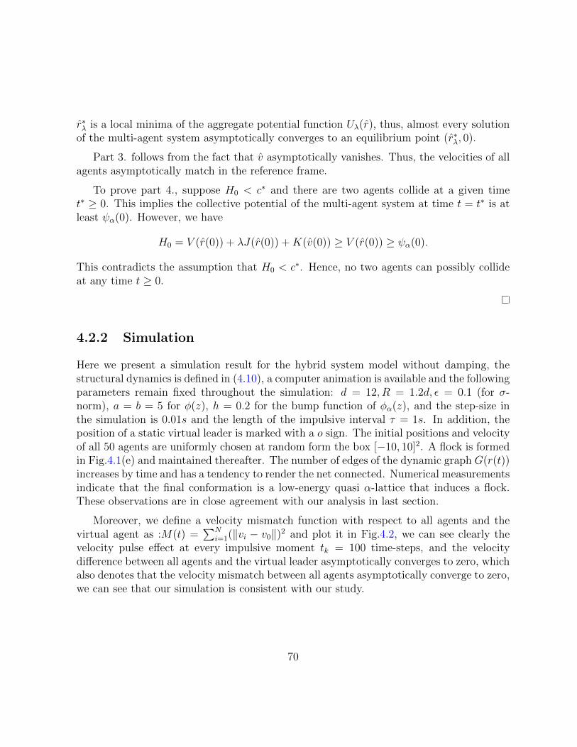
r∗λ is a local minima of the aggregate potential function Uλ(r), thus, almost every solutionof the multi-agent system asymptotically converges to an equilibrium point (r∗λ, 0).
Part 3. follows from the fact that v asymptotically vanishes. Thus, the velocities of allagents asymptotically match in the reference frame.
To prove part 4., suppose H0 < c∗ and there are two agents collide at a given timet∗ ≥ 0. This implies the collective potential of the multi-agent system at time t = t∗ is atleast ψα(0). However, we have
H0 = V (r(0)) + λJ(r(0)) +K(v(0)) ≥ V (r(0)) ≥ ψα(0).
This contradicts the assumption that H0 < c∗. Hence, no two agents can possibly collideat any time t ≥ 0.
4.2.2 Simulation
Here we present a simulation result for the hybrid system model without damping, thestructural dynamics is defined in (4.10), a computer animation is available and the followingparameters remain fixed throughout the simulation: d = 12, R = 1.2d, ε = 0.1 (for σ-norm), a = b = 5 for φ(z), h = 0.2 for the bump function of φα(z), and the step-size inthe simulation is 0.01s and the length of the impulsive interval τ = 1s. In addition, theposition of a static virtual leader is marked with a o sign. The initial positions and velocityof all 50 agents are uniformly chosen at random form the box [−10, 10]2. A flock is formedin Fig.4.1(e) and maintained thereafter. The number of edges of the dynamic graph G(r(t))increases by time and has a tendency to render the net connected. Numerical measurementsindicate that the final conformation is a low-energy quasi α-lattice that induces a flock.These observations are in close agreement with our analysis in last section.
Moreover, we define a velocity mismatch function with respect to all agents and thevirtual agent as :M(t) =
∑Ni=1(‖vi − v0‖)2 and plot it in Fig.4.2, we can see clearly the
velocity pulse effect at every impulsive moment tk = 100 time-steps, and the velocitydifference between all agents and the virtual leader asymptotically converges to zero, whichalso denotes that the velocity mismatch between all agents asymptotically converge to zero,we can see that our simulation is consistent with our study.
70
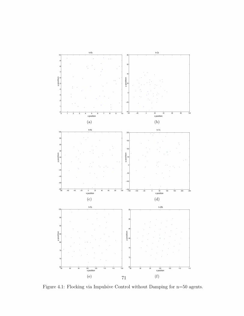
0 1 2 3 4 5 6 7 8 9 100
1
2
3
4
5
6
7
8
9
10
x position
y p
osit
ion
t=0s
(a)
−40 −20 0 20 40 60 80 100−40
−20
0
20
40
60
80
x position
y p
osit
ion
t=2s
(b)
−80 −60 −40 −20 0 20 40 60 80 100−80
−60
−40
−20
0
20
40
60
80
100
x position
y p
osit
ion
t=4s
(c)
−150 −100 −50 0 50 100 150 200 250−150
−100
−50
0
50
100
150
200
x position
y p
osit
ion
t=1s
(d)
85 90 95 100 105 110 115 12065
70
75
80
85
90
95
100
x position
y p
osit
ion
t=5s
(e)
85 90 95 100 105 110 11565
70
75
80
85
90
95
x position
y p
osit
ion
t=20s
(f)
Figure 4.1: Flocking via Impulsive Control without Damping for n=50 agents.
71
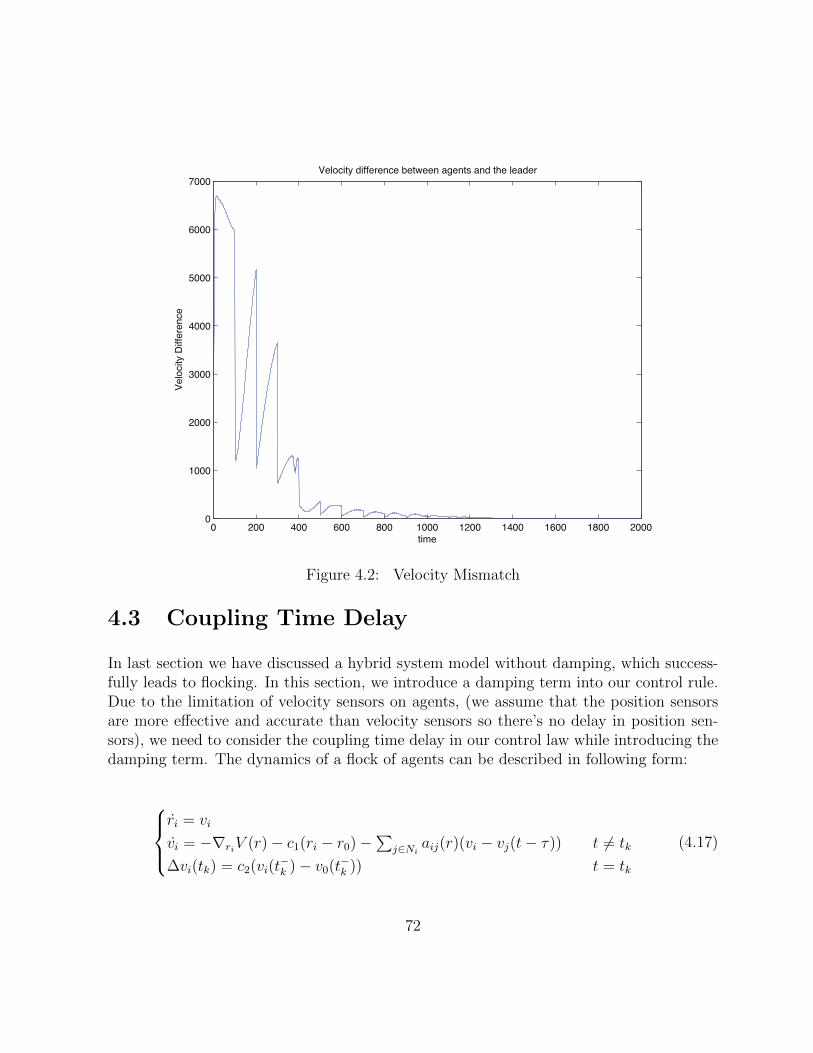
0 200 400 600 800 1000 1200 1400 1600 1800 20000
1000
2000
3000
4000
5000
6000
7000
time
Velocity difference between agents and the leaderV
elo
city D
iffe
ren
ce
Figure 4.2: Velocity Mismatch
4.3 Coupling Time Delay
In last section we have discussed a hybrid system model without damping, which success-fully leads to flocking. In this section, we introduce a damping term into our control rule.Due to the limitation of velocity sensors on agents, (we assume that the position sensorsare more effective and accurate than velocity sensors so there’s no delay in position sen-sors), we need to consider the coupling time delay in our control law while introducing thedamping term. The dynamics of a flock of agents can be described in following form:
ri = vi
vi = −∇riV (r)− c1(ri − r0)−∑
j∈Ni aij(r)(vi − vj(t− τ)) t 6= tk
∆vi(tk) = c2(vi(t−k )− v0(t−k )) t = tk
(4.17)
72
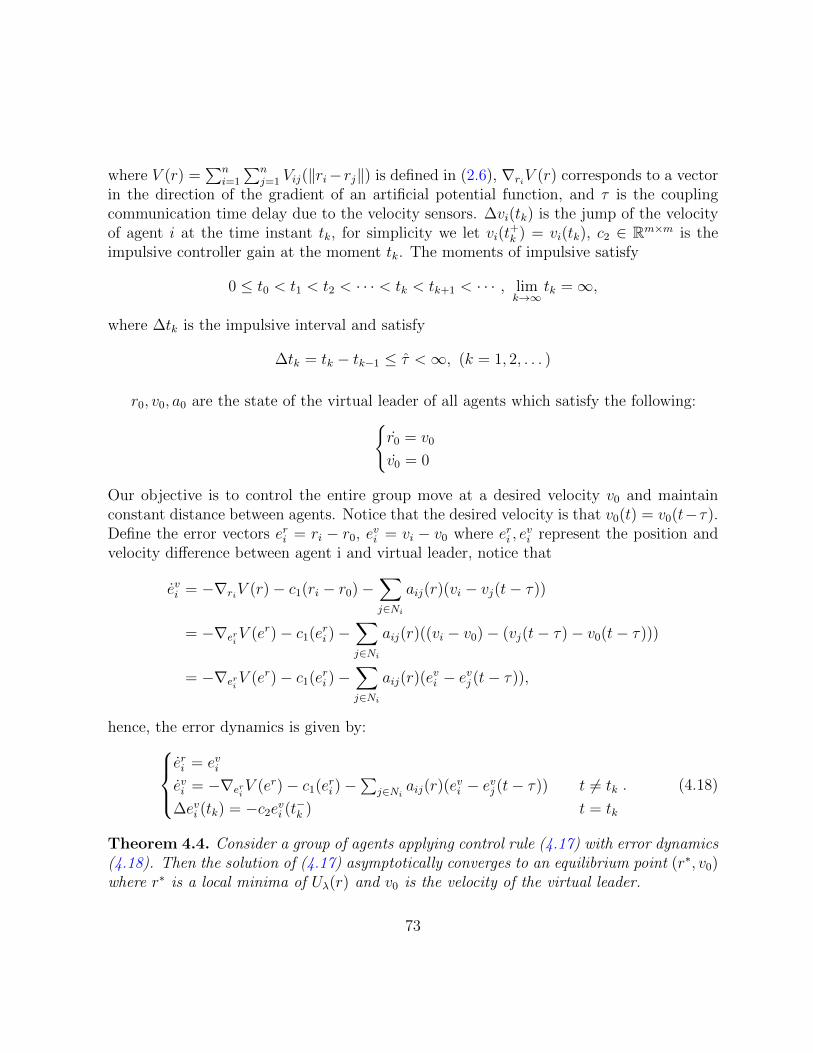
where V (r) =∑n
i=1
∑nj=1 Vij(‖ri− rj‖) is defined in (2.6), ∇riV (r) corresponds to a vector
in the direction of the gradient of an artificial potential function, and τ is the couplingcommunication time delay due to the velocity sensors. ∆vi(tk) is the jump of the velocityof agent i at the time instant tk, for simplicity we let vi(t
+k ) = vi(tk), c2 ∈ Rm×m is the
impulsive controller gain at the moment tk. The moments of impulsive satisfy
0 ≤ t0 < t1 < t2 < · · · < tk < tk+1 < · · · , limk→∞
tk =∞,
where ∆tk is the impulsive interval and satisfy
∆tk = tk − tk−1 ≤ τ <∞, (k = 1, 2, . . . )
r0, v0, a0 are the state of the virtual leader of all agents which satisfy the following:r0 = v0
v0 = 0
Our objective is to control the entire group move at a desired velocity v0 and maintainconstant distance between agents. Notice that the desired velocity is that v0(t) = v0(t−τ).Define the error vectors eri = ri − r0, evi = vi − v0 where eri , e
vi represent the position and
velocity difference between agent i and virtual leader, notice that
evi = −∇riV (r)− c1(ri − r0)−∑j∈Ni
aij(r)(vi − vj(t− τ))
= −∇eriV (er)− c1(eri )−
∑j∈Ni
aij(r)((vi − v0)− (vj(t− τ)− v0(t− τ)))
= −∇eriV (er)− c1(eri )−
∑j∈Ni
aij(r)(evi − evj (t− τ)),
hence, the error dynamics is given by:eri = evievi = −∇eri
V (er)− c1(eri )−∑
j∈Ni aij(r)(evi − evj (t− τ)) t 6= tk
∆evi (tk) = −c2evi (t−k ) t = tk
. (4.18)
Theorem 4.4. Consider a group of agents applying control rule (4.17) with error dynamics(4.18). Then the solution of (4.17) asymptotically converges to an equilibrium point (r∗, v0)where r∗ is a local minima of Uλ(r) and v0 is the velocity of the virtual leader.
73

Proof. For t ∈ [tk−1, tk), consider the following positive semi-definite Lyapunov function:
W =1
2
N∑i=1
(evi )T evi + V (er) +
c12
N∑i=1
(eri )T (eri ) +
1
2
N∑i=1
N∑j=1
aij(r)
∫ t
t−τ(evi (s))
T (evi (s))ds,
for any t ∈ [tk−1, tk), the right and upper Dini’s derivative of W along the trajectory of(4.18) is:
D+W =N∑i=1
(evi )T [−∇eri
V (er)− c1eri −∑j∈Ni
aij(r)(evi − evj (t− τ))] +
N∑i=1
(∇eriV (er))T evi
+ c1
N∑i=1
(eri )T evi +
1
2
N∑i=1
N∑j=1
aij(r)[(evi (t))
T evi (t)− (evi (t− τ))T evi (t− τ)]
=−N∑i=1
N∑j=1
aij(r)[(evi (t))
T (evi (t)− evj (t− τ))]
+1
2
N∑i=1
N∑j=1
aij(r)[(evi (t)
T )(evi (t))− (evi (t− τ))T (evi (t− τ))]
=N∑i=1
N∑j=1
aij(r)[−1
2(evi (t))
T (evi (t)) + (evi (t))T (evj (t− τ))− 1
2(evi (t− τ))T (evi (t− τ))]
= −1
2
N∑i=1
N∑j=1
aij(r)[evi (t)− evj (t− τ)]T [evi (t)− evj (t− τ)] ≤ 0.
Hence, for all t ∈ [tk−1, tk), W (t) < W (tk−1) for all evi (t) 6= evj (t − τ), moreover, it follows
74
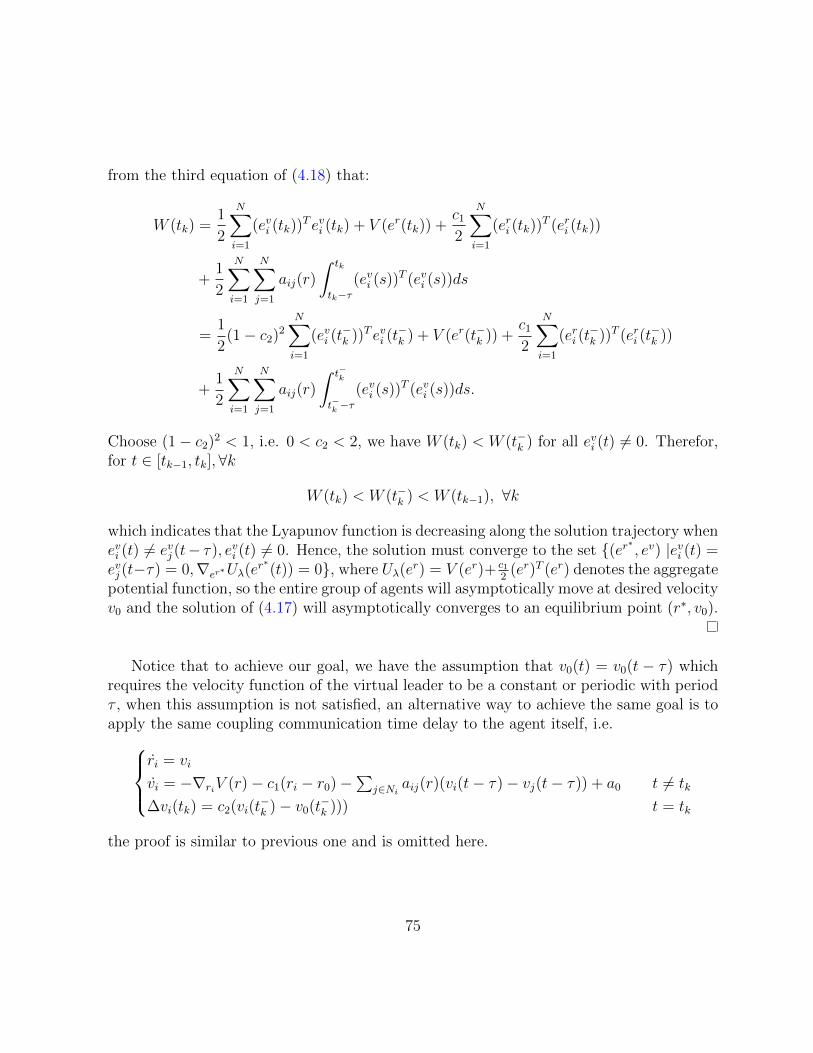
from the third equation of (4.18) that:
W (tk) =1
2
N∑i=1
(evi (tk))T evi (tk) + V (er(tk)) +
c12
N∑i=1
(eri (tk))T (eri (tk))
+1
2
N∑i=1
N∑j=1
aij(r)
∫ tk
tk−τ(evi (s))
T (evi (s))ds
=1
2(1− c2)2
N∑i=1
(evi (t−k ))T evi (t
−k ) + V (er(t−k )) +
c12
N∑i=1
(eri (t−k ))T (eri (t
−k ))
+1
2
N∑i=1
N∑j=1
aij(r)
∫ t−k
t−k −τ(evi (s))
T (evi (s))ds.
Choose (1− c2)2 < 1, i.e. 0 < c2 < 2, we have W (tk) < W (t−k ) for all evi (t) 6= 0. Therefor,for t ∈ [tk−1, tk],∀k
W (tk) < W (t−k ) < W (tk−1), ∀k
which indicates that the Lyapunov function is decreasing along the solution trajectory whenevi (t) 6= evj (t− τ), evi (t) 6= 0. Hence, the solution must converge to the set (er∗ , ev) |evi (t) =evj (t−τ) = 0,∇er∗Uλ(e
r∗(t)) = 0, where Uλ(er) = V (er)+ c1
2(er)T (er) denotes the aggregate
potential function, so the entire group of agents will asymptotically move at desired velocityv0 and the solution of (4.17) will asymptotically converges to an equilibrium point (r∗, v0).
Notice that to achieve our goal, we have the assumption that v0(t) = v0(t − τ) whichrequires the velocity function of the virtual leader to be a constant or periodic with periodτ , when this assumption is not satisfied, an alternative way to achieve the same goal is toapply the same coupling communication time delay to the agent itself, i.e.
ri = vi
vi = −∇riV (r)− c1(ri − r0)−∑
j∈Ni aij(r)(vi(t− τ)− vj(t− τ)) + a0 t 6= tk
∆vi(tk) = c2(vi(t−k )− v0(t−k ))) t = tk
the proof is similar to previous one and is omitted here.
75
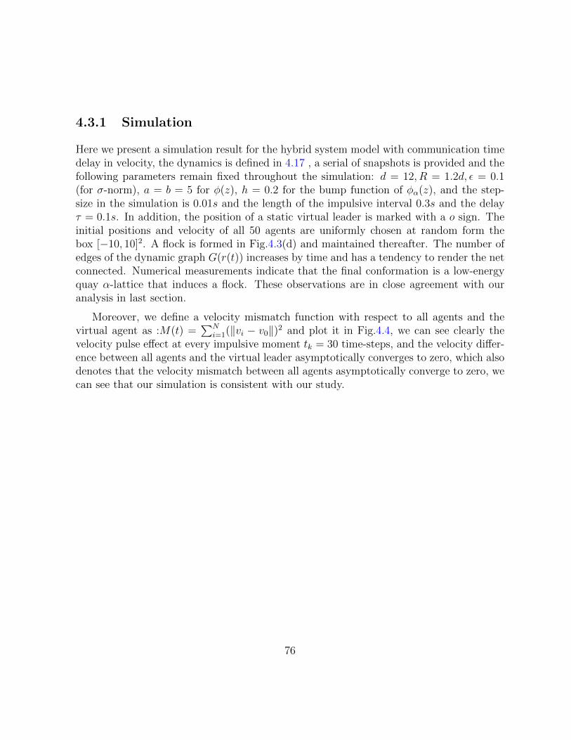
4.3.1 Simulation
Here we present a simulation result for the hybrid system model with communication timedelay in velocity, the dynamics is defined in 4.17 , a serial of snapshots is provided and thefollowing parameters remain fixed throughout the simulation: d = 12, R = 1.2d, ε = 0.1(for σ-norm), a = b = 5 for φ(z), h = 0.2 for the bump function of φα(z), and the step-size in the simulation is 0.01s and the length of the impulsive interval 0.3s and the delayτ = 0.1s. In addition, the position of a static virtual leader is marked with a o sign. Theinitial positions and velocity of all 50 agents are uniformly chosen at random form thebox [−10, 10]2. A flock is formed in Fig.4.3(d) and maintained thereafter. The number ofedges of the dynamic graph G(r(t)) increases by time and has a tendency to render the netconnected. Numerical measurements indicate that the final conformation is a low-energyquay α-lattice that induces a flock. These observations are in close agreement with ouranalysis in last section.
Moreover, we define a velocity mismatch function with respect to all agents and thevirtual agent as :M(t) =
∑Ni=1(‖vi − v0‖)2 and plot it in Fig.4.4, we can see clearly the
velocity pulse effect at every impulsive moment tk = 30 time-steps, and the velocity differ-ence between all agents and the virtual leader asymptotically converges to zero, which alsodenotes that the velocity mismatch between all agents asymptotically converge to zero, wecan see that our simulation is consistent with our study.
76
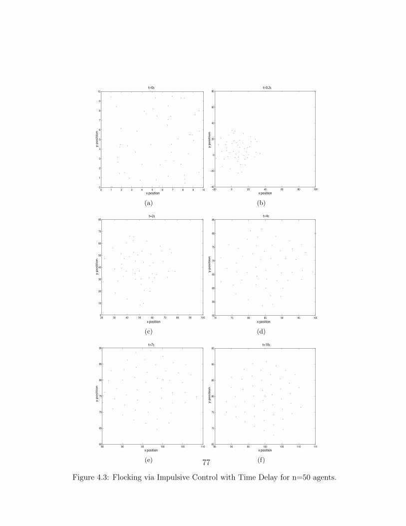
0 1 2 3 4 5 6 7 8 9 100
1
2
3
4
5
6
7
8
9
10
x position
y p
osit
ion
t=0s
(a)
−20 0 20 40 60 80 100−40
−20
0
20
40
60
80
x position
y p
osit
ion
t=0.2s
(b)
20 30 40 50 60 70 80 90 1000
10
20
30
40
50
60
70
80
x position
y p
osit
ion
t=2s
(c)
70 75 80 85 90 95 10050
55
60
65
70
75
80
85
x position
y p
osit
ion
t=4s
(d)
85 90 95 100 105 11060
65
70
75
80
85
90
x position
y p
osit
ion
t=7s
(e)
85 90 95 100 105 110 11565
70
75
80
85
90
95
x position
y p
osit
ion
t=10s
(f)
Figure 4.3: Flocking via Impulsive Control with Time Delay for n=50 agents.
77
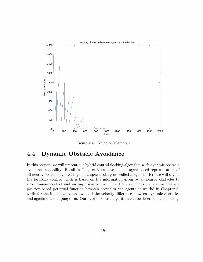
0 200 400 600 800 1000 1200 1400 1600 1800 20000
500
1000
1500
2000
2500
3000
3500
4000
4500
time
Velocity difference between agents and the leaderV
elo
city D
iffe
ren
ce
Figure 4.4: Velocity Mismatch
4.4 Dynamic Obstacle Avoidance
In this section, we will present our hybrid control flocking algorithm with dynamic obstacleavoidance capability. Recall in Chapter 3 we have defined agent-based representation ofall nearby obstacle by creating a new species of agents called β-agents. Here we will dividethe feedback control which is based on the information given by all nearby obstacles toa continuous control and an impulsive control. For the continuous control we create aposition-based potential function between obstacles and agents as we did in Chapter 3,while for the impulsive control we add the velocity difference between dynamic obstaclesand agents as a damping term. Our hybrid control algorithm can be described as following:
78
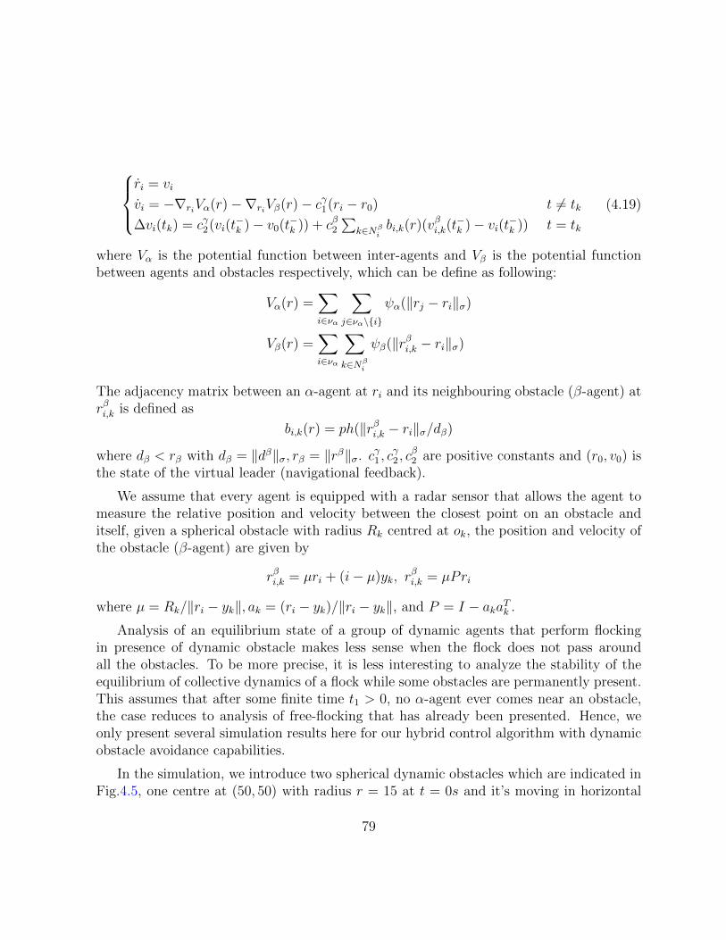
ri = vi
vi = −∇riVα(r)−∇riVβ(r)− cγ1(ri − r0) t 6= tk
∆vi(tk) = cγ2(vi(t−k )− v0(t−k )) + cβ2
∑k∈Nβ
ibi,k(r)(v
βi,k(t
−k )− vi(t−k )) t = tk
(4.19)
where Vα is the potential function between inter-agents and Vβ is the potential functionbetween agents and obstacles respectively, which can be define as following:
Vα(r) =∑i∈να
∑j∈να\i
ψα(‖rj − ri‖σ)
Vβ(r) =∑i∈να
∑k∈Nβ
i
ψβ(‖rβi,k − ri‖σ)
The adjacency matrix between an α-agent at ri and its neighbouring obstacle (β-agent) atrβi,k is defined as
bi,k(r) = ph(‖rβi,k − ri‖σ/dβ)
where dβ < rβ with dβ = ‖dβ‖σ, rβ = ‖rβ‖σ. cγ1 , cγ2 , c
β2 are positive constants and (r0, v0) is
the state of the virtual leader (navigational feedback).
We assume that every agent is equipped with a radar sensor that allows the agent tomeasure the relative position and velocity between the closest point on an obstacle anditself, given a spherical obstacle with radius Rk centred at ok, the position and velocity ofthe obstacle (β-agent) are given by
rβi,k = µri + (i− µ)yk, rβi,k = µPri
where µ = Rk/‖ri − yk‖, ak = (ri − yk)/‖ri − yk‖, and P = I − akaTk .
Analysis of an equilibrium state of a group of dynamic agents that perform flockingin presence of dynamic obstacle makes less sense when the flock does not pass aroundall the obstacles. To be more precise, it is less interesting to analyze the stability of theequilibrium of collective dynamics of a flock while some obstacles are permanently present.This assumes that after some finite time t1 > 0, no α-agent ever comes near an obstacle,the case reduces to analysis of free-flocking that has already been presented. Hence, weonly present several simulation results here for our hybrid control algorithm with dynamicobstacle avoidance capabilities.
In the simulation, we introduce two spherical dynamic obstacles which are indicated inFig.4.5, one centre at (50, 50) with radius r = 15 at t = 0s and it’s moving in horizontal
79
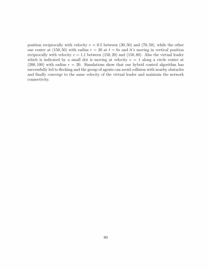
position reciprocally with velocity v = 0.5 between (30, 50) and (70, 50), while the otherone centre at (150, 50) with radius r = 20 at t = 0s and it’s moving in vertical positionreciprocally with velocity v = 1.1 between (150, 20) and (150, 80). Also the virtual leaderwhich is indicated by a small dot is moving at velocity v = 1 along a circle centre at(200, 100) with radius r = 20. Simulations show that our hybrid control algorithm hassuccessfully led to flocking and the group of agents can avoid collision with nearby obstaclesand finally converge to the same velocity of the virtual leader and maintain the networkconnectivity.
80
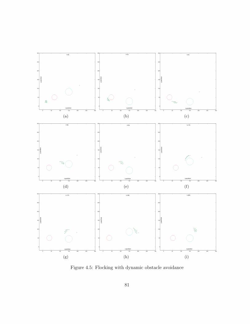
0 50 100 150 200 250 300
0
50
100
150
200
250
300
x position
y p
osi
tio
n
t=0s
(a)
0 50 100 150 200 250 300
0
50
100
150
200
250
300
x position
y p
osi
tio
n
t=3s
(b)
0 50 100 150 200 250 300
0
50
100
150
200
250
300
x position
y p
osi
tio
n
t=5s
(c)
0 50 100 150 200 250 300
0
50
100
150
200
250
300
x position
y p
osi
tio
n
t=8s
(d)
0 50 100 150 200 250 300
0
50
100
150
200
250
300
x position
y p
osi
tio
n
t=9s
(e)
0 50 100 150 200 250 300
0
50
100
150
200
250
300
x position
y p
osi
tio
n
t=13s
(f)
0 50 100 150 200 250 300
0
50
100
150
200
250
300
x position
y p
osi
tio
n
t=17s
(g)
0 50 100 150 200 250 300
0
50
100
150
200
250
300
x position
y p
osi
tio
n
t=30s
(h)
0 50 100 150 200 250 300
0
50
100
150
200
250
300
x position
y p
osi
tio
n
t=60s
(i)
Figure 4.5: Flocking with dynamic obstacle avoidance
81
Chapter 5
Conclusion and Future Direction
Flocking is a form of collective behaviour of large number of interacting agents with acommon group objective. For many decades, scientists from many diverse disciplines in-cluding animal behaviour, physics and biophysics, social sciences, and computer sciencehave been fascinated by the emergence of flocking in groups of agents via local interactions[19, 42, 41, 40, 37, 47, 59, 56, 52, 35, 27, 57, 39, 45]. Coordinated motion has receivedsignificant recent attention in cooperative robotics (i.e., to make the agents to aggregateand stay in a tight group, achieve a spatial pattern or a geometric formation, or tack amoving object [45]) and biology (i.e., formation of fruiting bodies by bacteria, foragingbehaviour of ants, or cohesive flight of warms of bees [41, 37]). Such problems are alsoclosely related to a group reaching a consensus or agreement (since often preference canbe linked to position[44]). The problem of distributed agreement is a problem which hasbeen popular in the multi-agent dynamical systems community.
Dynamics of multi-agent systems can exhibit rich and complex characteristics. Com-bining agent, sensing, and communication characteristics results in a multi-scale systemwith local spatio-temporal agent action dynamically combining into an “emergent” globalpattern of group behaviour [23]. There are other problems such as task allocation orscheduling, executing spatially distributed tasks, or task execution under time or energy orother constraints. For example, task allocation often raised in multi-agent dynamical sys-tem problems where the “tasks” arise via interactions with the environment, and the tasksmust be allocated across the agents and properly scheduled in time for efficient execution,methods from distributed scheduling, load balancing, and assignment are integrated intocoordinated motion methods to achieve a multi-objective method that mush balance tightgroup cohesion with the pressing need to complete tasks. This thesis is concerned withthe coordinated motion of the group of agents to migrate to certain destination, or track a
82
group leader,while network connectivity is maintained and both inter-agent and obstaclescollision avoidance capabilities are ensured, both continuous and impulsive control havebeen considered to achieve these goals.
In chapter 2, we firstly introduce some basic concepts in graph theory in order to estab-lish a theoretical framework for modelling the flocking problem for multi-agent dynamicalsystem, then we study the discrete model given by Vicsek [59], in which the agents of thesystem applying a very simple rule by averaging the velocity of their neighbouring agentsplus some random noise, simulation results show that under low noise and high densitysituation agents can achieve a global consensus of velocity by using only local informationof neighbours, this discrete model gives us a first impression of what consists flocking formulti-agent dynamical systems. Moreover, we present a continuous model of double inte-grator agents using the Newton’s law, and how to design the potential function betweenthe agents, which is main method we use to denote the inter-agent interactions in thisthesis. In chapter 3, we study the continuous model for flocking for multi-agent dynamicalsystems, by introducing a virtual leader into our model, we successfully eliminate the frag-mentation phenomenon and ensure network connectivity of the system at the same time.Lyapunov techniques for continuous system has been used to prove the asymptotic sta-bility of the equilibrium state of the system, communication time delay is also consideredin our model. At the end of chapter 2 we give a detailed investigation on how to modelthe obstacles in the environment and present an algorithm to allow the agents to possessobstacle avoidance capabilities. In chapter 4, we further extend the existing continuousmodel to a hybrid control model, which is a more general model for flocking problem formulti-agent dynamical systems, and this chapter is the main contribution of this thesis.We use the velocity feedbacks given by the virtual leader as impulsive controls while thepotential function between agents as the continuous controls, and our model successfullylead to flocking, by applying this hybrid control method we find out that we can removethe damping terms which appear in the continuous control model in chapter 3, hence, wecan effectively reduce the influence subjected to sensing time delay in velocity and reducethe cost as well. Lyapunov techniques for continuous and impulsive systems is used andstability analysis is also provided. At the end of this chapter we present a hybrid controlalgorithm to allow agents to possess dynamic obstacle avoidance capabilities, simulationresults illustrate our algorithm is in agreement with our analysis.
Further, we can study the stability criteria for our hybrid control model for flockingwith dynamic obstacle avoidance capabilities, and obstacles other than a stripe or sphericalcan be constructed in the future. It is not difficult to imagine that given a non-convexobstacle there might be multiple β-agents which are equally close to an agent. Assumingthat all of these β-agents repel an agent in the system, one might expect that in certain
83
situations there would be a conflict of tasks between obstacle avoidance by a group ofagents and achieving a group objective by a virtual leader. An example of this might bethe agent, obstacle (β-agent) and the virtual are located on a same line, or the agentsare trapped by a convex obstacle. In these cases, the agents can not pass through the“wall” and reach their destination. Hence, further study of using a more sophisticatedobstacle avoidance approach eliminates getting trapped behind an obstacle can be donein the future. A successful example of such approach is the use of gyroscopic forces forobstacle avoidance in [7, 8]. The influence of random perturbation in the environment canalso be considered in the future.
Study on flocking with predictive mechanisms can also be investigated in the future.In [32] the authors present a discrete-time MPC flocking protocol to estimated futureposition of neighbours. This model successfully improve the convergent speed comparedwith Olfati-Saber’s model and achieve a better quasi α-lattice structure. In [51] the authorsuse a game theory approach to multi-agent team cooperation to ensure team cooperationby considering a combination of individual costs as a team cost function. Optimizationalgorithms and formation controls other than α-lattice can also be considered.
84

APPENDICES
85
Appendix A
Convergent Analysis for Vicsek’sModel
Before studying the stability of Vicsek’s model, we need to introduce some concepts inmatrix analysis which will be very useful in the later on proof.
Definition A.1. Nonegative Matrix Let A = [aij]m×n, A is said to be a nonnegativematrix (A ≥ 0) if all aij ≥ 0, positive matrix (A > 0) if all aij > 0.
Definition A.2. Primitive Matrix A nonnegative matrix A ∈ Rn×n is said to beprimitive if and only if Am > 0 for some m ≥ 1.
Definition A.3. Stochastic Matrix A nonnegative matrix A ∈ Rn×n with the propertythat all its row sums are 1 is said to be a (row) stochastic matrix. (since each row may bethought of as a discrete probability distribution on a sample space with n points).
Definition A.4. Ergodic A stochastic matrix A ∈ Rn×n with the property that limi→∞Mi
is a matrix of rank 1 is called ergodic.
Theorem A.1. Primitive stochastic matrices are ergodic.
Theorem A.2. Let M1,M2, . . . ,Mm be a finite set of ergodic matrices with the propertythat for each sequence Mi1 ,Mi2 , . . . ,Mij of positive length, the matrix product MijMij−1
, . . . ,Mi1
is ergodic. Then for each infinite sequence, Mi1 ,Mi2 , . . . there exist a row vector c suchthat
limj→∞MijMij−1· · ·Mi1 = 1c
86
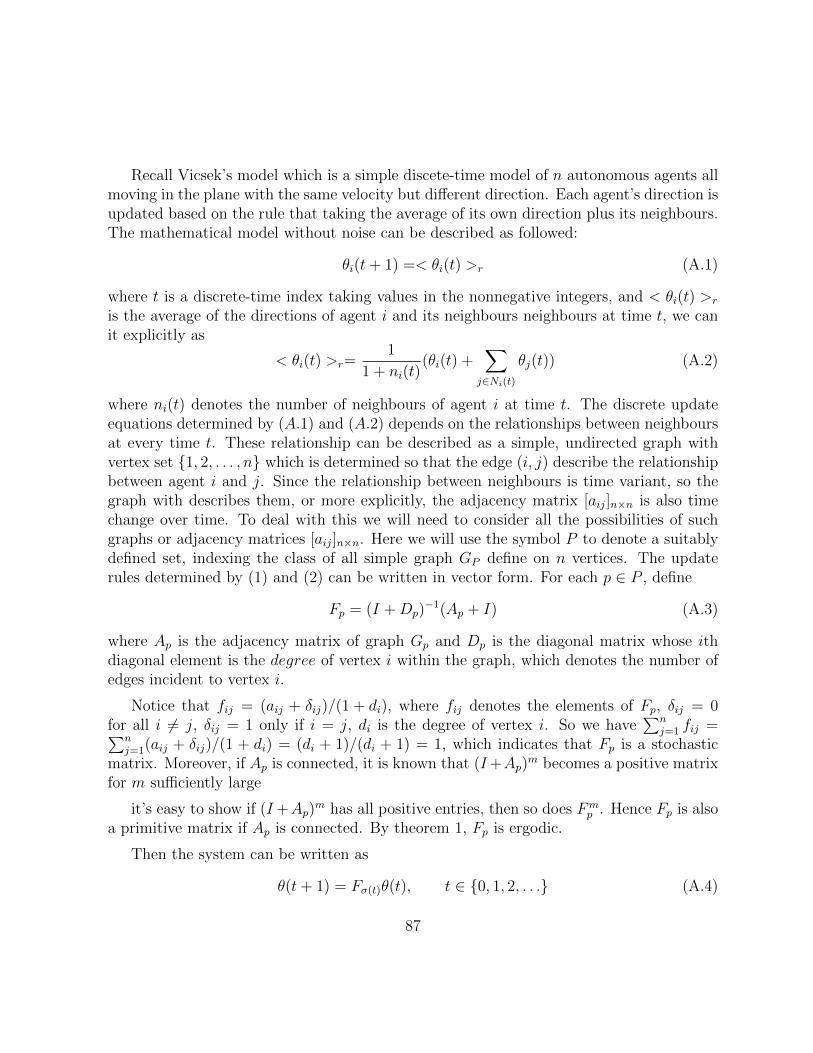
Recall Vicsek’s model which is a simple discete-time model of n autonomous agents allmoving in the plane with the same velocity but different direction. Each agent’s direction isupdated based on the rule that taking the average of its own direction plus its neighbours.The mathematical model without noise can be described as followed:
θi(t+ 1) =< θi(t) >r (A.1)
where t is a discrete-time index taking values in the nonnegative integers, and < θi(t) >r
is the average of the directions of agent i and its neighbours neighbours at time t, we canit explicitly as
< θi(t) >r=1
1 + ni(t)(θi(t) +
∑j∈Ni(t)
θj(t)) (A.2)
where ni(t) denotes the number of neighbours of agent i at time t. The discrete updateequations determined by (A.1) and (A.2) depends on the relationships between neighboursat every time t. These relationship can be described as a simple, undirected graph withvertex set 1, 2, . . . , n which is determined so that the edge (i, j) describe the relationshipbetween agent i and j. Since the relationship between neighbours is time variant, so thegraph with describes them, or more explicitly, the adjacency matrix [aij]n×n is also timechange over time. To deal with this we will need to consider all the possibilities of suchgraphs or adjacency matrices [aij]n×n. Here we will use the symbol P to denote a suitablydefined set, indexing the class of all simple graph GP define on n vertices. The updaterules determined by (1) and (2) can be written in vector form. For each p ∈ P , define
Fp = (I +Dp)−1(Ap + I) (A.3)
where Ap is the adjacency matrix of graph Gp and Dp is the diagonal matrix whose ithdiagonal element is the degree of vertex i within the graph, which denotes the number ofedges incident to vertex i.
Notice that fij = (aij + δij)/(1 + di), where fij denotes the elements of Fp, δij = 0for all i 6= j, δij = 1 only if i = j, di is the degree of vertex i. So we have
∑nj=1 fij =∑n
j=1(aij + δij)/(1 + di) = (di + 1)/(di + 1) = 1, which indicates that Fp is a stochasticmatrix. Moreover, if Ap is connected, it is known that (I+Ap)
m becomes a positive matrixfor m sufficiently large
it’s easy to show if (I+Ap)m has all positive entries, then so does Fm
p . Hence Fp is alsoa primitive matrix if Ap is connected. By theorem 1, Fp is ergodic.
Then the system can be written as
θ(t+ 1) = Fσ(t)θ(t), t ∈ 0, 1, 2, . . . (A.4)
87
where θ is the direction vector θ = [θ1 θ2 · · · θn]′and σ : 0, 1, . . . → P is a switching signalwhose value at time t denotes the index of the graph representing the agents’ relationshipat time t.
In our stability analysis we want to show that for a large class of switching signals, orany initial condition, the directions of all the agents in the systems will finally converge toa same steady state direction θss, which is equivalent to write
limt→∞
θ(t) = θss1 (A.5)
where 1 = [1 1 · · · 1]′n×1 . Intuitively this can not always be true unless we have someadditional conditions on the connectivity of the Graph Gσ(t) , to show this let’s considertwo extreme situations:
1. the interaction range r is very small so that there is at least one agent, say i, whichnever acquires any neighbours. Mathematically this means the graph Gσ(t) is neverconnected and vertex i is isolated for all t.
2. the interaction range r is large enough that it ensures every agent in the system caninteract with all other agents for all t. Mathematically this means the graph Gσ(t) isconnected and σ(t) is fixed for all t.
In situation 1, since there’s at least one agent can never interact with any other agents,such that the systems state θ can not converge to the steady state θss for certain initialconditions, in situation 2 convergence of of θ to θss1 can easily be established because withσ fixed, (A.5) is a linear, time-invariant, discrete-time system. So the most interestingsituation is between these two extremes when σ changes with time, Gσ(t) is not necessarilyconnected for all t, but no strictly proper subsets of Gσ(t)’s vertices is isolated from the restfor all t. Motivated by this idea, we will introduce a new concept called jointly connected,which is a weaker condition than connected of a graph.
Definition A.5. Jointly Connected Let G be the union of a collection of simply graphsGp1 , Gp2 , . . . , Gpm, which means G with vertex set V and edge set E equaling the union ofthe edge sets of all the graphs in the collection. We say that such a collection Gp1 , Gp2 , . . . , Gpmis jointly connected if the union G of its members is a connected graph.
Definition A.6. Linked Together N agents are called linked together across a time inter-val [t, τ ] if the collection of graph Gσ(t), Gσ(t+1), . . . , Gσ(τ) encountered along the intervalis jointly connected.
88
Notice that if n agents is jointly connected, then situation 1 is included while situation2 is eliminated, then we can establish the sufficient condition for the convergence of thesystem to a stead state.
Theorem A.3. Let θ(0) be fixed and let σ : 0, 1, 2, . . . → P be a switching signal forwhich there exists an infinite sequence of contiguous, nonempty, bounded, time-intervals[ti, ti+1), i ≥ 0, starting at t0 = 0, with the property that across each such interval, the nagents are linked together. Then
limt→∞
θ(t) = θss1 (A.6)
where θss is a number depending only on θ(0) and σ.
Before proving theorem 3, we need two more lemmas.
Lemma A.1. Let m ≥ 2 be a positive integer and let A1, A2, . . . , Am be nonnegative n×nmatrices. Suppose that the diagonal elements of all of the Ai are positive and let u and ρdenote the smallest and largest of these, respectively. Then
A1A2 · · ·Am ≥ (µ2
2ρ)m−1(A1 + A2 + · · ·+ Am). (A.7)
Proof. Let δ = µ2/2ρ. It will be shown by induction that
A1A2 · · ·Am ≥ δi−1(A1 + A2 + · · ·+ Ai) (A.8)
holds for i ∈ 2, 3, . . . ,m. Toward this end, note that it’s possible to write each Ai asAi = µI +Bi where Bi is nonnegative. Then, for any j, k ∈ 1, 2, . . . ,m
AjAk = (µI +Bj)(µI +Bk) = µ2I + µ(Bj +Bk) +BjBk.
Hence
AjAk ≥ µ2I + µ(Bj +Bk) ≥ µ2I + µ2
2ρ(BjBk) = δ((ρI +Bj) + (ρI +Bk))
Since (ρI +Bj) ≥ Aj and (ρI +Bk) ≥ Ak it follows that
AjAk ≥ δ(Aj + Ak) ∀j, k ∈ 1, 2, . . . ,m. (A.9)
89
Setting j = 1 and k = 2 proves that (A.8) holds for i = 2. Now suppose that m > 2and that (8) hold for i ∈ 2, 3, . . . , l where l is some integer in 2, 3, . . . ,m − 1. ThenA1A2 · · ·Al+1 = (A1, . . . , Al)Al+1 so by the inductive hypothesis
A1A2 · · ·Al+1 ≥ δl−1(A1 + A2 + · · ·+ Al)Al+1 (A.10)
However, using (A.9) l times, we can write
(A1 + A2 + · · ·+ Al)Al+1 ≥ δ((A1 + Al+1) + (A2 + Al+1) + · · ·+ (Al + Al+1)).
Thus
(A1 + A2 + · · ·+ Al)Al+1 ≥ δ(A1 + A2 + · · ·+ Al+1)
This and (A.10) imply that (A.8) holds for i = l+1. Therefore, by induction the statementis true for all i ∈ 2, 3, . . . ,m
Lemma A.2. Let p1, p2, . . . , pm be a set of indices in P for which Gp1 , Gp2 , . . . , Gpmis a jointly connected collection of graphs. Then the matrix product Fp1Fp2 , · · · , Fpm isergodic.
Proof. Let F = (I + D)−1(I + A) where A and D are respectively the adjacency ma-trix and diagonal degree matrix of the union of the collection of graphs P for whichGp1 , Gp2 , . . . , Gpm. Since the collection is jointly connected, its union is connected whichmeans F is connected, so F is primitive. By Lemma 1,
Fp1Fp2 · · ·Fpm ≥ γ(Fp1 + Fp2 + · · ·+ Fpm) (A.11)
where γ is a positive constant depending on the matrices in the product. Since for i ∈1, 2, . . . ,m, Fpi = (I + Dpi)
−1(I + Api) and D > Dpi , it must have that Fpi ≥ (I +D)−1(I + Api), i ∈ 1, 2, . . . ,m. From this and (A.11) it follows that
Fp1Fp1 · · ·Fpm ≥ γ(I +D)−1(mI + Ap1 + Ap2 + · · ·+ Apm) (A.12)
However, Ap1 + Ap2 + · · ·+ Apm ≥ A and mI ≥ I so
Fp1Fp1 · · ·Fpm ≥ γF
Since the product Fp1Fp1 · · ·Fpm is bounded below by a primitive matrix γF , the productmust be primitive as well, moreover, Fp1Fp1 · · ·Fpm is also a stochastic matrix, so it mustbe ergodic.
90

Then we can are ready to prove theorem 3 now,
Proof. Let T denote the least upper bound on the lengths of the intervals [ti, ti+1), i ≥ 0.By assumption T < ∞. Let Φ(t, t) = I, t ≥ 0, and Φ(t, τ) , Fσt−1 · · ·Fστ+1Fστ , t > τ ≥ 0.Clearly θ(t) = Φ(t, 0)θ(0). To complete the theorem’s proof, it’s enough to show that
limt→∞
Φ(t, 0) = 1c (A.13)
for some row vector c since this would imply (A.6) with θss , cθ(0). In view of Lemma2, the constraints on σ imply that each such matrix product Φ(tj+1, tj), j ≥ 0, is ergodic.Moreover the set of possible Φ(tj+1, tj), j ≥ 0, must be finite because each Φ(tj+1, tj) isa product of at most T matrices from Fp : p ∈ P which is a finite set. But Φ(tj, 0) =Φ(tj, tj−1)Φ(tj−1, tj−2), . . . ,Φ(t1, t0). Therefor by theorem 2
limj→∞
Φ(tj, 0) = 1c (A.14)
which is equivalent to (A.13).
91
References
[1] I. Akyildiz, W. Su, Y. Sankarasubramniam, and E. Cayirci. A survey on sensornetworks. IEEE Communications Magazine, pages 102–114, 2002.
[2] R. Bachmayer and N. E. Leonard. Vehicle networks for gradient descent in a sampledenvironment. In Conf. Decision Contr., pages 112–117, Las Vegas, Nevada, December2002.
[3] T. Balch and R. C. Arkin. Behaviour-based formation control for multirobot teams.IEEE Trans. on Robotics and Automation, 14(6):926–939, 1998.
[4] G. Beni and P. Liang. Pattern reconfiguration in swarms-convergence of a distributedasynchronous and bounded iterative algorithm. IEEE Trans. on Robotics and Au-tomation, 12(3):485–490, 1996.
[5] B. Bollobas. Modern Graph Theory, volume 184 of Fraduate Texts in Mathematics.Springer-Verlag, 1998.
[6] C. M. Breder. Equations descriptive of fish schools and other animal aggregations.Ecology, 35(3):361–370, 1954.
[7] D. E. Chang and J. Marsden. Gyroscopic forces and sollision avoidance. In Conferencein Honor of A. J. Krener’s 60th Birthday, 2002.
[8] D. E. Chang, S. Shadden, J. Marsden, and R. Olfati-Saber. Collision avoidance formultiple agent systems. In IEEE Conf. on Decision and Control, December 2003.
[9] Z. Csahok and T. Vicsek. Lattices-gas model for collective biological motion. PhysicalReveiw E, 52(5):5297–5303, 1995.
92
[10] A. Czirok, A. L. Barabasi, and T. Vicsek. Collective motion of self-propelled particles:Kinetic phase transition in one dimension. Physical Review Letters, 82(1):209–212,1999.
[11] A. Czirok, E. Ben-Jacob, I. Cohen, and T. Vicsek. Formation of complex bacterialcolonies via self-generated vortices. Physical Reveiw E, 54(2):1791–1801, 1996.
[12] A. Czirok, H. E. Stanley, and T. Vicsek. Spontaneously ordered motion of self-propelled particles. Journal of Physics A: Mathematical, Nuclear and General,30:1375–1385, 1997.
[13] A. Czirok and T. Vicsek. Collective behabiour of interacting self-propelled particles.Physica A, 281:17–29, 2000.
[14] J. P. Desai, J. Ostrowski, and V. Kumar. controlling formations of multiple mobilerobots. In IEEE International Conference on Robotics and Automation, pages 2864–2869, Leuven, Belgium, 1988.
[15] J. P. Desai, J. Ostrowski, and V. Kumar. Modelling and control of formations ofnonholonomic mobile robots. IEEE Trans. on Robotics and Automation, 17(6):905–908, 2001.
[16] R. Diestel. Graph Theory, volume 173 of Graduate Texts in Mathematics. Springer-Verlag, 2000.
[17] M. Egerstedt and X. Hu. Formation constrained multi-agent control. IEEE Trans. onRobotics and Automation, 17(6):947–951, 2001.
[18] P. Erdos and A. Hajnal. On chromatic number of infinite graphs. Theory of Graphs,pages 83–98, 1968.
[19] E.Shaw. Fish in schools. Natural History, 84(8):40–45, 1975.
[20] M. Fiedler. Algebraic connectivity of graphs. Czechoslovak Mathematical Journal,23(98):298–305, 1973.
[21] P. Frindrod. Models of individual aggregation or clustering in single and multi-speciescommunities. Journal of Mathematical Biology, 26:651–660, 1988.
[22] D. Frunbaum and A. Okubo. Modeling social animal aggregations In: Frontiers inTheoretical Biology., volume 100. Springer, New York, 1994.
93
[23] Veysel Gazi and Kevin M. Passino. Swarm stability and optimization. Springer, 2010.
[24] F. Giulietti, L. Pollini, and M. Innocenti. Autonomous formation flight. IEEE ControlSystems Magazine, 20(6):34–44, 2000.
[25] C. Godsil and G. Royle. Algebraic Graph Theory, volume 207 of Graduate Texts inMathematics. Springer, 2001.
[26] S. Gueron and S. A. Levin. The dynamics of group formation. Mathematical Bio-sciences, 128:243–264, 1995.
[27] D. Helbing, I. Farkas, and T. Vicsek. Simulation dynamical features of escape panic.Nature, 407:487–490, 2000.
[28] Tanner G. Herbert, Ali Jadbabaie, and J. G. Pappas. Flocking in fixed and switchingnetworks. IEEE Trans. on Automatic Control, 52(5):863–868, 2007.
[29] R. A. Horn and C. R. Johnson. Matrix Analysis. Cambridge University Press, 1987.
[30] A. Jadbabaie, J. Lin, and A. S. Morese. Coordination of groups of mobile agents usingnearest neighbor rules. IEEE Trans. on Automatic Control, 48(6):988–1001, 2003.
[31] K. Jin, P. Liang, and G. Beni. Stability of synchronized distributed control of discreteswarm structures. In IEEE International Conference on Robotics and Automation,pages 1033–1038, San Diego, California, May 1994.
[32] Zhan Jingyuan and Li Xiang. Flocking of multi-agent systems with predictive mech-anisms. In 18th IFAC World Congress, 2011.
[33] N. E. Leonard and E. Fiorelli. Virtual leaders, artificial potentials and coordinatedcontrol of groups. In Conf. Decision Contr., pages 2968–2973, Orlando, FL, December2001.
[34] M. Lizana and V. Padron. A specially discrete model for aggregating populations.Journal of Mathematical Biology, 38:79–102, 1999.
[35] A. Mogilner and L. Edelstein-Keshet. A non-local model for a swarm. J. Math.Biology, 38:534–570, 1999.
[36] P. Ogren, M. Egerstedt, and X. Hu. A control lyapunov function approach to multi-agent coordination. In Conf. Decision Contr., pages 1150–1155, Orlando, FL, Decem-ber 2001.
94
[37] A. Okubo. Dynamical aspects of animal grouping: Swarms, schools, flocks and herds.Adv. Biophysics, 22:1–94, 1986.
[38] R. Olfati-Saber. Flocking with obstacle avoidance. In Technical Report 2003-2006,Control and Dynamical Systems, Pasadena, California, February 2003. California In-stitute of Technology.
[39] J. K. Parrish, S. V. Viscido, and D. Grunbaum. Self-organized fish schools: andexamination of emergent properties. Biol. Bull, 202:296–305, 2002.
[40] B. L. Partridge. The structure and function of fish schools. Scientific American,246(6):114–123, 1982.
[41] B. L. Partridge. The chorus-line hypothesis of maneuver in avian flocks. Nature,309:344–345, 1984.
[42] T. J. Pitcher, B. L. Partridge, and C. S. Wardle. A blind fish can school. ScientificAmerican, 194(4268):963–965, 1976.
[43] M. M. Polycarpou, Y. Yang, and K. M. Passino. Cooperative control of distributedmulti-agent systems. IEEE Control Systems Magazine, 1999.
[44] Z. Qing, C. Shihua, and Y. Changchun. Impulsive consensus problem of second-ordermulti-agent systems with switching topologies. Communications in Nonlinear Scienceand Numerical Simulation, 17:9–16, 2012.
[45] Olfati-Saber R. Flocking for multi-agent dynamic systems: algorithms and theory.IEEE Trans. Automat. Control, 51:401–420, 2006.
[46] E. M. Rauch, M. M. Millonas, and D. R. Chialvo. Pattern formation and functionalityin swarm models. Physics Letters A, 207:185–193, 1995.
[47] C. W. Reynolds. Flocks, herds, and school: a distributed behavioural model. ComputerGraphics CACM SIGGRAPH’ 87, 21(4):25–34, 1987.
[48] C. W. Reynolds. Steering behaviours for autonomous characters. In Game DevelopersConference, pages 763–782, San Francisco, CA, 1999. Miller Freeman Game Group.
[49] C. W. Reynolds. Interaction with a group of autonomous characters. In Game De-velopers Conference, pages 449–460, San Francisco, CA, 2000. CMP Game MediaGroup.
95
[50] R. O. Saber and R. M. Murray. Flocking with obstacle avoidance: cooperation withlimited communication in mobile networks. In 42nd IEEE Conference on Decisionand Control, volume 2, pages 2022–2028, December 2003.
[51] E. Semsar-Kazerooni and K. Khorasani. A game theory approach to multi-agent teamcooperation. In 2009 American Control Conference, pages 4512–4518, Hyatt RegencyRiverfront, St. Louis, MO, USA, June 2009.
[52] N. Shimoyama, K. Sugawara, T. mizuguchi, Y. Hayakawa, and M. Sano. Collectivemotion in a system of motile elements. Physical Review Letters, 76(20):3870–3873,1996.
[53] I. Suzuki and M. Yamashita. Distributed anonymous mobile robots: Formation ofgeometric patterns. SIAM Journal on Computing, 28(4):1347–1363, 1999.
[54] H. G. Tanner. Stable flocking of mobile agents. In 42nd IEEE Conference on Decisionand Control, volume 2, pages 2016–2021, December 2003.
[55] J. Toner and Y. Tu. Long-range order in a two-dimensional dynamical xy model: Howbirds fly together. Physical Review Letters, 75(23):4326–4329, 1995.
[56] J. Toner and Y. Tu. Flocks, herds, and schools: A quantitative theory of flocking.Physical Reveiw E, 58(4):4828–4858, October 1998.
[57] T. Vicsek. A question of scal. Nature, 411:421–421, 2001.
[58] T. Vicsek, A. Czirok, I. J. Farkas, and D. Helbing. Application of statistical mechanicsto collective motion in biology. Physica A, 274:182–189, 1999.
[59] T. Vicsek, A. Czirook, E. Ben-Jacob, O. Cohen, and I. Shochet. Novel tiype of phasetransition in a system of self-driven particles. Physical Review Letters, 75(6):1226–1229, August 1995.
[60] K. Warburton and J. Lazarus. Tendency-distance models of social cohesion in animalgroups. Journal of Theoretical Biology, 150:473–488, 1991.
[61] H. Yamaguchi. A cooperative hunting behaviour by mobile-robot troops. The inter-national Journal of Robotics Research, 18(8):931–940, 1999.
[62] Zhengquan Yang, Qing Zhang, Zuolian Jiang, and Zengqiang Chen. Flocking of multi-agents with time delay. International Journal of Systems Science, 56:46–75, 2011.
96

[63] L. P. Zhang and H. B. Jiang. Impulsive generalized synchronization for a class of non-linear discrete chaotic systems. Communications in Nonlinear Science and NumericalSimulation, 16:2027–2032, 2011.
97