Embed Size (px)
Citation preview

International Journal of
Environmental Research
and Public Health
Article
Flood-Exposure Is Associated with Higher Prevalenceof Child Undernutrition in Rural Eastern IndiaJose Manuel Rodriguez-Llanes 1,*, Shishir Ranjan-Dash 2,3, Alok Mukhopadhyay 4 andDebarati Guha-Sapir 1
1 Centre for Research on the Epidemiology of Disasters, Institute of Health and Society,Université catholique de Louvain, Brussels 1200, Belgium; [email protected]
2 Department of Management, Siksha ‘O’ Anusandhan University, Bhubaneswar 751003, India;[email protected]
3 Tata Trusts, Mumbai 400001, India4 Voluntary Health Association of India, New Delhi 110016, India; [email protected]* Correspondence: [email protected]; Tel.: +32-2764-3372
Academic Editor: Jan C. SemenzaReceived: 22 December 2016; Accepted: 2 February 2016; Published: 15 February 2016
Abstract: Background: Child undernutrition and flooding are highly prevalent public health issues inAsia, yet epidemiological studies investigating this association are lacking. Methods: To investigateto what extent floods exacerbate poor nutritional status in children and identify most vulnerablegroups, we conducted a population-based survey of children aged 6–59 months inhabiting floodedand non-flooded communities of the Jagatsinghpur district, Odisha (India), one year after large floodsin 2008. Anthropometric measurements on 879 children and child, parental and household levelvariables were collected through face-to-face interviews in September 2009. The association betweenflooding and the prevalence of wasting, stunting and underweight was examined using weightedmultivariate logistic regression for children inhabiting communities exposed solely to floods in 2008and those communities repeatedly flooded (2006 and 2008) controlling for parental education andother relevant variables. We examined the influence of age on this association. Propensity scorematching was conducted to test the robustness of our findings. Results: The prevalence of wastingamong children flooded in 2006 and 2008 was 51.6%, 41.4% in those flooded only in 2008, and21.2% in children inhabiting non-flooded communities. Adjusting by confounders, the increasedprevalence relative to non-flooded children in the exposed groups were 2.30 (adjusted prevalenceratio (aPR); 95% CI: 1.86, 2.85) and 1.94 (95% CI: 1.43, 2.63), respectively. Among repeatedly floodedcommunities, cases of severe wasting in children were 3.37 times more prevalent than for childreninhabiting in those non-flooded (95% CI: 2.34, 4.86) and nearly twice more prevalent relative tothose flooded only once. Those children younger than one year during previous floods in 2006showed the largest difference in prevalence of wasting compared to their non-flooded counterparts(aPR: 4.01; 95% CI: 1.51, 10.63). Results were robust to alternative adjusted models and in propensityscore matching analyses. For similar analyses, no significant associations were found for childstunting, and more moderate effects were observed in the case of child underweight. Conclusions:Particularly in low-resource or subsistence-farming rural settings, long-lasting nutritional responsein the aftermath of floods should be seriously considered to counteract the long-term nutritionaleffects on children, particularly infants, and include their mothers on whom they are dependent.The systematic monitoring of nutritional status in these groups might help to tailor efficient responsesin each particular context.
Keywords: flood; disaster; malnutrition; vulnerability; climate change; child; infant; wasting
Int. J. Environ. Res. Public Health 2016, 13, 210; doi:10.3390/ijerph13020210 www.mdpi.com/journal/ijerph

Int. J. Environ. Res. Public Health 2016, 13, 210 2 of 20
1. Introduction
In the last decade alone, floods have affected nearly one billion people worldwide [1]. Despite theirpotential burden to society, the consequences of floods on human health remain rarely investigated, andthe few studies that do suggest increased short-term risks of mortality, injury, certain communicablediseases and psychosocial trauma [2–4]. Our understanding of the long-term health consequencesof flooding and recurrent floods is even more limited [2,3,5]. Moreover, the impacts of flooding onnutritional health are likely to be quite severe among young children in developing countries [6–8].Multiple mechanisms explaining how floods may lead to poor nutrition in these settings have beenproposed [9,10].
Floods can severely disrupt livelihoods, especially in low-resource settings [7,8]. Floodedhouseholds are affected by a plethora of adverse conditions including food insecurity due to cropfailure or food affordability due to sudden price changes [7,9]. Daily care of children and breastfeedingpractices is importantly challenged during floods as in worst scenarios all basic services becomedisrupted, including water and sanitation conditions, or the provision of community basic health andsocial services [7–11]. In addition, diarrhea or respiratory diseases, which occur at increased ratesduring or after flooding [2,3] have the potential to worsen child nutritional status [11].
Notably, most of the global burden of child undernutrition is clustered in south Asia andsub-Saharan Africa [11]. In Asia alone, Black et al., estimated 96 million cases of stunted children (thosepresenting growth failure) and additional 36 million of wasting cases (abnormal thinness indicating aprocess of weight loss) in children younger than five in 2011 [11]. Moreover, Asia is particularly proneto flood hazards [12]. In 2011 alone, nearly 130 million people were affected by flooding [1], of whichat least 11 million might be estimated children under five [13].
These nutritional problems in children might be seriously aggravated by the augmented likelihoodof extreme precipitation events and flooding due to climate change [14] but also by increasingsocial and physical vulnerability to flood hazards [15]. In particular, children’s higher susceptibilityto climate-related hazards [16] coupled with climate-related food insecurity in many developingeconomies [17] might increase the burden of disease due to flooding, jeopardizing human developmentof future generations [11].
Sound evidence on the association of flooding and child nutrition is still rare and population-basedstudies are lacking [2,3]. Despite national and international NGOs, and international healthorganizations have claimed for years the consequences of floods on nutritional health of the mostvulnerable, far-reaching change on both tailored prevention and response policies will require soundscientific evidence.
The state of Odisha, surrounding the Bay of Bengal, is prone to numerous hazards, such as floods,droughts or cyclones, but the floods that occurred in September 2008 were unprecedented in theirimpact [18]. Overall, 4.5 million people were affected by flooding, with severe losses and disruption offishing activities, livestock, silk and crop farming. Drinking water supplies were importantly affectedby the flood. Schools, front-line care and social services were challenged to operate normally [19].Anganwadi centres were also damaged. These are important community resources, as they areused as shelter in case of disaster and provide service to 0–6 year old children and pregnant andlactating mothers under the Integrated Child Development Scheme (ICDS). The government providedemergency relief packages among the affected populations, including food and basic utilities tochildren and adults, covering their basic needs for the first 15 days following the floods [18].
Here we sought to examine the association between flooding and child undernutrition in anepidemiological, controlled rural population-based study representative of 17,876 children aged 6 to59 months conducted in September 2009. We assessed children affected solely by the 2008 flood and byrepeated flooding in 2006 and 2008 and investigated the most vulnerable child cohorts through theinteraction of flood exposure with child’s age.
Int. J. Environ. Res. Public Health 2016, 13, 210 3 of 20
2. Materials and Methods
2.1. Analysis Plan
Our study focused on the differences in relevant anthropometric indicators (i.e., stunting andwasting) between flooded and non-flooded populations. Our second research objective reviewedthese differences for the prevalence of moderate and severe undernutrition indicators. We additionallyprovided population-weighted estimates of the prevalence of stunting, wasting and underweight inthe overall, flooded and non-flooded surveyed populations. We investigated the nutrition of childcohorts affected by floods in 2006 and 2008, and those children affected only by floods in 2008. An ageinteraction was examined to investigate the most vulnerable age groups to the effects of floods, as thisproved to be relevant on a previous study [7].
As our primary aim was to estimate the effect of flooding on child undernutrition, we excludedvariables (e.g., caregiving practices, food security, and access to health care, water and sanitation,diarrheal morbidities) which may have mediated this effect [20]. We supported this selection byexamining the data collected on these variables framed within the UNICEF conceptual malnutritionframework [21]. Overall, 51 variables were assessed. Out of these, 18 plausible mediators wereexcluded. The remaining 33 variables were assessed as possible confounders [22]. We also tested if thefrequencies of the 33 variables varied across flooded and non-flooded communities [23]. Two adjustedmodels were proposed, one controlling for confounders, another adjusting for confounders in additionto other variables which differed across exposure.
2.2. Exposure Data
The list of flooded villages during the 2006 and 2008 events in the four selected blocks wasobtained from the Odisha State Disaster Mitigation Authority, OSDMA [24]. The estimated percentageof affected population within each of the 122 villages was also provided. Exposure to flooding wasdefined as living in a village flooded in 2008. Overall, nearly 90% of the population was estimated asdirectly affected by the floods in these villages (mean = 92.5%; SEM = 1.5). An additional 143 villageswere unaffected by this flood and located in the same blocks, and were used as the comparison group.For the 2006 flood event, OSDMA reported 110 villages as flooded in the same four blocks, witha majority of these (n = 101, 92%) also affected in 2008. The data was provided as the estimatedpercentage of the population affected by the floods within each village. This was used in controlledanalyses but did not affect the study design.
2.3. Study Design and Participants
Jagatsinghpur is a coastal district located in the state of Odisha, eastern India. It has a populationof one million with around 90% residing in rural areas [25]. The region is located in a large floodplain which is part of the Himalayan system and is subject to heavy monsoons and recurrent flooding.The district has been severely hit by five major floods in the last decade, the one following the cycloneParadip (05B) in 1999, followed by heavy floods in 2001, 2003 and 2006. In our study area, villageshave been only affected by 1999 cyclone Paradip before the 2006 floods. The latest floods, starting inmid-September 2008, produced great devastation [1,18].
We used a population-based cross-sectional design to estimate the association of exposure toflooding in 2008 with the prevalence of child undernutrition one year later in rural Jagatsinghpurdistrict, Odisha, India. A two-stage cluster survey was required to obtain a probability sample of900 children aged 6 to 59 months representing children of this age in 265 villages located in fourseverely flood-affected blocks of the district (Kujang, Biridi, Balikuda, Tirtol). Of these, 122 have beenflooded and 143 non-flooded in September 2008. The percentage of households flooded in each villagewas obtained for 2006 and 2008 events from OSDMA.
At the first sampling stage, 30 clusters (29 villages) were selected with probability proportional totheir size. At the second sample stage we did a census on children living in each selected village which

Int. J. Environ. Res. Public Health 2016, 13, 210 4 of 20
allowed us to randomly select children. This design is useful if the population of interest is clustered invillages and the information on the population itself is limited [26]. The Primary Sampling Units (PSUs)were the villages and the Secondary Sampling Unit (SSU) were the children. We considered a 30 (PSU)by 30 (SSU) design, which should provide a probability sample of 900 children. We firstly listed all265 villages with their population size projected for 2009 from the available census [24]. Subsequentlywe selected 30 clusters (29 villages) out of the 265 listed with probability proportional to its population.Village population size ranged between 7 and 9430 inhabitants. Probability Proportionate to Size(PPS) sampling with replacement (e.g., one large village was selected twice) was used to select villageswith unequal size and give an equal probability to each child in the population of being selected [26].Second, within each selected village an updated list of eligible children (i.e., a 6 to 59 month old childliving in the surveyed village at time of interview) was obtained from the ICDS centers (1 ICDS centerfor every 1000 inhabitants) and validated with the ward members of each village. In all 3671 eligiblechildren were listed from 29 villages during the month preceding the training and piloting of thequestionnaire. Once the lists were compiled, it was detected that three flooded villages (Korana,Jamphar and Raghunathpur) and two non-flooded (Muthapada, Sureilo) did not have enough eligiblechildren (less than 30). We therefore created five new clusters by merging the list of children in eachof these five villages (n = 280) with those of the closest non-selected flooded or non-flooded village,respectively, of our list (Figure A1). At the second stage of the sampling, thirty children per clusterwere randomly selected.
At the time of planning this research in April–June 2009, the only available information on thechildren population was that of the Indian census of 2001 [27]. We estimated the total populationand number of children living in these 265 villages using state-level population projections for 2009available at the census [27]. The total population living in these villages was estimated at 228,550.Using this method, we initially calculated that the survey would represent a population of roughly17,876 children aged 6 to 59 months living in flood-prone areas of Odisha.
The sample size required to answer our research question was calculated a priori usingOpenEpi [28]. Based on results from a previous study [7] we set a 15% difference in prevalence ofundernutrition, considering the prevalence in flooded communities would be 50% (35% in non-flooded).Setting a prevalence to 50% in the power calculation provides the largest sample size possible for anycombinations given the prevalence difference is constant, and thus provides conservative samples.For a power of 80% with α (error) = 0.05 and approximately equal samples of the compared groups, asample of 340 children (170 in each group) was required. We used a conservative design effect of 2 toadjust for a complex survey design. Overall, 680 children (340 in each group) were required to safelyanswer our research question. Accounting for maximum attrition in our sample of 25%, we planned tosample 900 children.
2.4. Ethical Considerations
Ethical approval was provided by the Community Health Ethics Committee, Voluntary HealthAssociation of India, New Delhi. All the participants involved in the study were informed about thenature of the study, research objectives and about confidentiality of the data, with the assurance thatnon-participation would not lead to negative consequences. Persons eligible to participate in the studywere not offered a monetary incentive for participation. Written informed consent was obtained forevery head of household visited. In case the respondent was illiterate, we asked a literate personfrom the community to read out the consent form and explain it to the head of the family. Then weobtained the thumb impression of the respondent. In those cases, the person who read the consent formalso signed as a witness. Research procedures were consistent with the Declaration of Helsinki [29].Interviews were administered after obtaining informed consent. The protocol was reviewed by a smallgroup of scientists who had experience working with survivors of natural disasters and amendedbased on their recommendations.

Int. J. Environ. Res. Public Health 2016, 13, 210 5 of 20
2.5. Procedures
We used three anthropometric indicators to assess malnutrition: stunting or chronic malnutritionexpressed as height-for-age, underweight as weight-for-age and wasting or acute malnutrition asweight-for-height. Weight measurements were undertaken to the nearest 100 g by trained researchassistants using a beam balance (<10 kg; Raman Surgical Co., Delhi, India) and an electronic balancefor those children heavier than 10 kg. For children younger than 2 years of age, length was measured tothe nearest millimeter in the recumbent position using an infantometer (Narang Medical, Delhi, India).Children older than 2 years were measured in standing position using an adjustable board calibratedin millimeters. We measured and weighed each child twice to minimize measurement errors and usethe average value of both measurements to gain precision. All instruments were calibrated daily.
The survey questionnaire used in this study was adapted from the core one developedand approved by a multidisciplinary consortium of researchers (i.e., sociologists, psychologists,epidemiologists, economists and public health scientists) working as part of the MICRODIS project.The instrument development was based on interim literature reviews, and closely followed theUNICEF conceptual framework on child malnutrition [21]. A survey questionnaire equivalent to ourswas successfully used in another site in India. The questionnaire was used to collect backgroundinformation at the household level, and more specifically from mothers and fathers, covering basicsocio-demographic characteristics, wealth, child caring practices, healthcare access, maternal andpaternal education, income and credit practices, water and sanitation, food consumption patterns;demographics, nutrition and health status data at the child level.
The questionnaires were administered by the Voluntary Health Association of India (VHAI),a non-profit organization which supports social and health-related country-wide initiatives. Twelveexperienced research assistants [7] received a three-day training on anthropometry and interviewprocedures in late August 2009. The questionnaire was piloted in 12 households (six in floodedvillages and six in non-flooded) and revised based on the pilot exercise. The final questionnaire wastranslated to the local language in Odisha (Oriya) and then back translated into English by differentprofessional translators and a researcher checked agreement between both versions. All interviewslasted 45–60 min. Field work was carried out between the 6th and 24th of September 2009.
2.6. Statistical Methods
ENA for SMART software (version November 2008) was used to calculate nutritional indicatorswith the 2006 World Health Organization Standard [30]. Missing data was rare: ten children withages out of range were excluded as well as two children with missing values for weight-for-height.Children from five additional villages not in the original PPS selection were not included in the finalanalysis as our study sample provided enough power to answer our main research question.
We examined the relationship between flood exposure and undernutrition in unadjustedand multiple adjusted logistic regression models with a quasi-binomial distribution to control foroverdispersion [23]. Confounders were variables associated with child nutrition statistically, having ap-value equal or lower than 0.2 starting with a full model using 33 relevant variables [22]. Backwardselection was used to get the final list of confounders for each nutritional indicator. At each stepthe non-significant variable with the largest p value was excluded to obtain a final model includingsignificant variables (i.e., p ď 0.2). Weighted Wald tests and t-tests (in the particular case of testingmean differences) were used to compare each variable distribution across flooded and non-floodedpopulations [23], with a significance level alpha of 0.2.
Results were provided as prevalence ratios, crude (PR) or adjusted (aPR) with 95% confidenceintervals. The two-way interaction of flood-exposure with the variable child age was examined.All tests were two-tailed with α = 0.05. All analyses were weighted. Weights were calculated as theinverse of the selection probabilities. Statistical analyses were conducted in R (Version 3.0.2) [31] withthe survey package [23]. To check for population differences across exposure or potential selectionbias, propensity score analysis was carried out with the package MatchIt [32]. The nearest neighbor
Int. J. Environ. Res. Public Health 2016, 13, 210 6 of 20
method was performed to match samples in flooded and non-flooded cohorts by similar covariatesdistributions as indicated by calculated propensity scores [32]. Reporting of the study followed theSTROBE guidelines (Table B1).
2.7. Estimates of Population Size
Through our survey data, we assessed the total children population aged 6 to 59 months livingin these 265 villages of Odisha. A total 16,791 children (95% CI: 15,979, 17,602) were estimated, with6810 children in the 122 flooded villages (95% CI: 6128, 7493) and 9,980 inhabiting the 143 non-floodedvillages (95% CI: 9043, 10,917). These estimates provide an idea of the population size to which thesubsequently presented findings apply.
3. Results
3.1. Sample and Determinants of Child Undernutrition in Flooded and Non-Flooded Communities
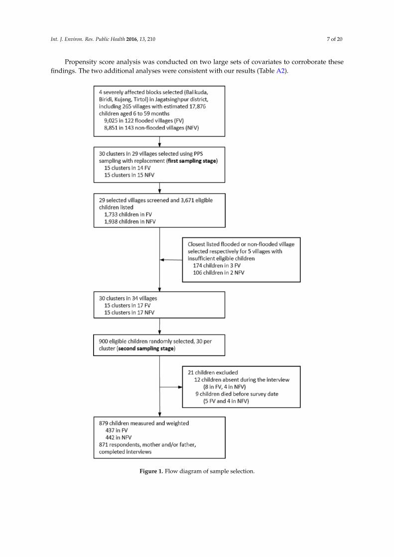
Out of 900 selected children, 21 could not be measured and were not replaced. Out of these,12 were not present at the time of the interview and were not found in the two additional visits totheir households. Of these cases, eight occurred in the flooded villages and the other four in thenon-flooded. In addition, nine children died within the period between the collection of the lists andthe day they were surveyed. Out of these children, five lived in flooded villages and the remainingfour in non-flooded (Figure 1). The overall response rate was 97.7% and consistent across flooded(97.1%) and non-flooded (98.2%) children’s parents.
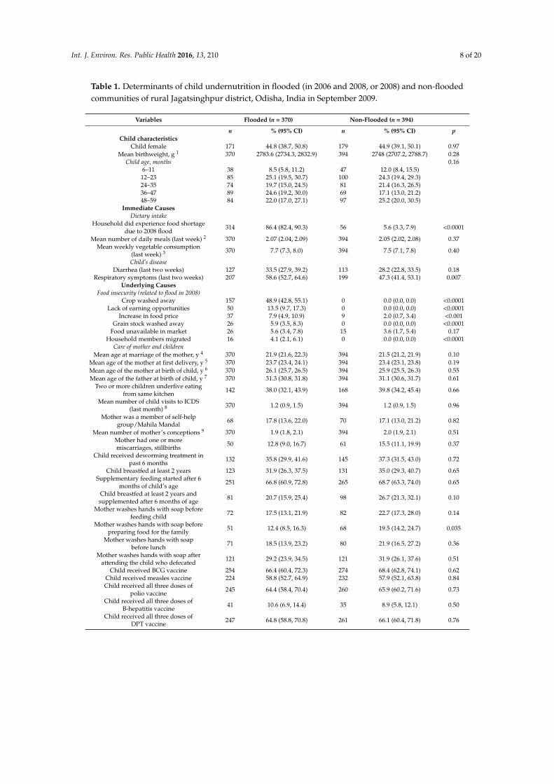
Baseline characteristics of mothers, fathers, children and households are presented in Table 1 andare classified according to broad categories in the UNICEF conceptual malnutrition framework [21].Overall, the distributions of a child’s age, the mother’s age at marriage and at first delivery,breastfeeding and complementary food practices, mother hand washing practices (i.e., before feedingthe child and before preparing food for the family), improved latrine, improved toilet, maternaleducation, paternal education, caste and owned land, all differed across flooded and non-floodedchildren populations.
3.2. Effect of Floods on Child Undernutrition
Overall, the prevalence of wasting was slightly higher in children of flooded communities in 2006and 2008 (Prev: 51.6; 95% CI: 45.0, 58.2) compared to those living in villages flooded in 2008 (Prev:41.4; 95% CI: 26.4, 56.4) but especially relative to those non-flooded (Prev: 21.2; 95% CI 15.8, 26.6).Crude and adjusted models showed consistent effect sizes for the associations (Table 2). Flooding wasmost significantly associated with wasting indicators, not with stunting and smaller effects, althoughstatistically significant, were observed for its association with underweight.
In models adjusted by confounders (Table A1), children repeatedly exposed to flooding in 2006and 2008 showed slightly larger aPRs for total wasting (2.30; 95% CI: 1.86, 2.85) but comparable to1.94 (95% CI: 1.43, 2.63) observed in those flooded exclusively in 2008. However, children additionallyexposed to floods in 2006 had more than a 3-times higher prevalence of severe wasting relative tothose non-flooded (aPR: 3.37; 95% CI: 2.34, 4.86) and nearly doubled that of those only exposed to 2008floods. The prevalence of moderate wasting was similar across the two exposed groups (Table 2).
3.3. Effect of Age on Undernutrition
Table 3 shows that age is an important covariate to consider in the final model, but only to modelthe children in communities repeatedly flooded. For those children, our analyses revealed specific agevulnerabilities related to previous flood experience. In particular, the cohort of children younger thanone year at times of previous floods in 2006 (in our study aged 36–47 months) were those presentingthe largest difference in prevalence of wasting compared to their non-flooded counterparts (aPR: 4.01;95% CI: 1.51, 10.63; p = 0.005).
Int. J. Environ. Res. Public Health 2016, 13, 210 7 of 20
Propensity score analysis was conducted on two large sets of covariates to corroborate thesefindings. The two additional analyses were consistent with our results (Table A2).
Figure 1. Flow diagram of sample selection.
Int. J. Environ. Res. Public Health 2016, 13, 210 8 of 20
Table 1. Determinants of child undernutrition in flooded (in 2006 and 2008, or 2008) and non-floodedcommunities of rural Jagatsinghpur district, Odisha, India in September 2009.
Variables Flooded (n = 370) Non-Flooded (n = 394)
n % (95% CI) n % (95% CI) pChild characteristics
Child female 171 44.8 (38.7, 50.8) 179 44.9 (39.1, 50.1) 0.97Mean birthweight, g 1 370 2783.6 (2734.3, 2832.9) 394 2748 (2707.2, 2788.7) 0.28
Child age, months 0.166–11 38 8.5 (5.8, 11.2) 47 12.0 (8.4, 15.5)
12–23 85 25.1 (19.5, 30.7) 100 24.3 (19.4, 29.3)24–35 74 19.7 (15.0, 24.5) 81 21.4 (16.3, 26.5)36–47 89 24.6 (19.2, 30.0) 69 17.1 (13.0, 21.2)48–59 84 22.0 (17.0, 27.1) 97 25.2 (20.0, 30.5)
Immediate CausesDietary intake
Household did experience food shortagedue to 2008 flood 314 86.4 (82.4, 90.3) 56 5.6 (3.3, 7.9) <0.0001
Mean number of daily meals (last week) 2 370 2.07 (2.04, 2.09) 394 2.05 (2.02, 2.08) 0.37Mean weekly vegetable consumption
(last week) 3 370 7.7 (7.3, 8.0) 394 7.5 (7.1, 7.8) 0.40
Child’s diseaseDiarrhea (last two weeks) 127 33.5 (27.9, 39.2) 113 28.2 (22.8, 33.5) 0.18
Respiratory symptoms (last two weeks) 207 58.6 (52.7, 64.6) 199 47.3 (41.4, 53.1) 0.007Underlying Causes
Food insecurity (related to flood in 2008)Crop washed away 157 48.9 (42.8, 55.1) 0 0.0 (0.0, 0.0) <0.0001
Lack of earning opportunities 50 13.5 (9.7, 17.3) 0 0.0 (0.0, 0.0) <0.0001Increase in food price 37 7.9 (4.9, 10.9) 9 2.0 (0.7, 3.4) <0.001
Grain stock washed away 26 5.9 (3.5, 8.3) 0 0.0 (0.0, 0.0) <0.0001Food unavailable in market 26 5.6 (3.4, 7.8) 15 3.6 (1.7, 5.4) 0.17
Household members migrated 16 4.1 (2.1, 6.1) 0 0.0 (0.0, 0.0) <0.0001Care of mother and children
Mean age at marriage of the mother, y 4 370 21.9 (21.6, 22.3) 394 21.5 (21.2, 21.9) 0.10Mean age of the mother at first delivery, y 5 370 23.7 (23.4, 24.1) 394 23.4 (23.1, 23.8) 0.19Mean age of the mother at birth of child, y 6 370 26.1 (25.7, 26.5) 394 25.9 (25.5, 26.3) 0.55Mean age of the father at birth of child, y 7 370 31.3 (30.8, 31.8) 394 31.1 (30.6, 31.7) 0.61
Two or more children underfive eatingfrom same kitchen 142 38.0 (32.1, 43.9) 168 39.8 (34.2, 45.4) 0.66
Mean number of child visits to ICDS(last month) 8 370 1.2 (0.9, 1.5) 394 1.2 (0.9, 1.5) 0.96
Mother was a member of self-helpgroup/Mahila Mandal 68 17.8 (13.6, 22.0) 70 17.1 (13.0, 21.2) 0.82
Mean number of mother’s conceptions 9 370 1.9 (1.8, 2.1) 394 2.0 (1.9, 2.1) 0.51Mother had one or moremiscarriages, stillbirths 50 12.8 (9.0, 16.7) 61 15.5 (11.1, 19.9) 0.37
Child received deworming treatment inpast 6 months 132 35.8 (29.9, 41.6) 145 37.3 (31.5, 43.0) 0.72
Child breastfed at least 2 years 123 31.9 (26.3, 37.5) 131 35.0 (29.3, 40.7) 0.65Supplementary feeding started after 6
months of child’s age 251 66.8 (60.9, 72.8) 265 68.7 (63.3, 74.0) 0.65
Child breastfed at least 2 years andsupplemented after 6 months of age 81 20.7 (15.9, 25.4) 98 26.7 (21.3, 32.1) 0.10
Mother washes hands with soap beforefeeding child 72 17.5 (13.1, 21.9) 82 22.7 (17.3, 28.0) 0.14
Mother washes hands with soap beforepreparing food for the family 51 12.4 (8.5, 16.3) 68 19.5 (14.2, 24.7) 0.035
Mother washes hands with soapbefore lunch 71 18.5 (13.9, 23.2) 80 21.9 (16.5, 27.2) 0.36
Mother washes hands with soap afterattending the child who defecated 121 29.2 (23.9, 34.5) 121 31.9 (26.1, 37.6) 0.51
Child received BCG vaccine 254 66.4 (60.4, 72.3) 274 68.4 (62.8, 74.1) 0.62Child received measles vaccine 224 58.8 (52.7, 64.9) 232 57.9 (52.1, 63.8) 0.84Child received all three doses of
polio vaccine 245 64.4 (58.4, 70.4) 260 65.9 (60.2, 71.6) 0.73
Child received all three doses ofB-hepatitis vaccine 41 10.6 (6.9, 14.4) 35 8.9 (5.8, 12.1) 0.50
Child received all three doses ofDPT vaccine 247 64.8 (58.8, 70.8) 261 66.1 (60.4, 71.8) 0.76
Int. J. Environ. Res. Public Health 2016, 13, 210 9 of 20
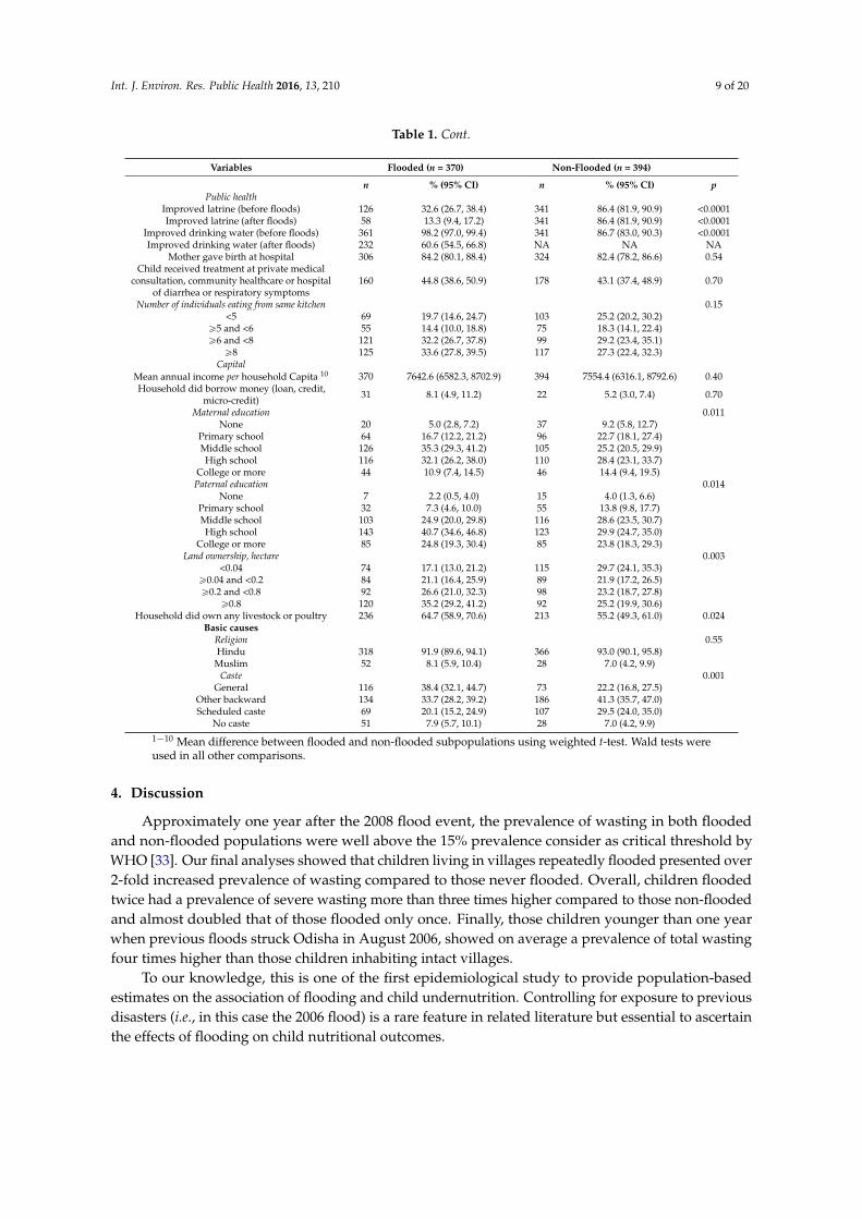
Table 1. Cont.
Variables Flooded (n = 370) Non-Flooded (n = 394)
n % (95% CI) n % (95% CI) pPublic health
Improved latrine (before floods) 126 32.6 (26.7, 38.4) 341 86.4 (81.9, 90.9) <0.0001Improved latrine (after floods) 58 13.3 (9.4, 17.2) 341 86.4 (81.9, 90.9) <0.0001
Improved drinking water (before floods) 361 98.2 (97.0, 99.4) 341 86.7 (83.0, 90.3) <0.0001Improved drinking water (after floods) 232 60.6 (54.5, 66.8) NA NA NA
Mother gave birth at hospital 306 84.2 (80.1, 88.4) 324 82.4 (78.2, 86.6) 0.54Child received treatment at private medical
consultation, community healthcare or hospitalof diarrhea or respiratory symptoms
160 44.8 (38.6, 50.9) 178 43.1 (37.4, 48.9) 0.70
Number of individuals eating from same kitchen 0.15<5 69 19.7 (14.6, 24.7) 103 25.2 (20.2, 30.2)
ě5 and <6 55 14.4 (10.0, 18.8) 75 18.3 (14.1, 22.4)ě6 and <8 121 32.2 (26.7, 37.8) 99 29.2 (23.4, 35.1)
ě8 125 33.6 (27.8, 39.5) 117 27.3 (22.4, 32.3)Capital
Mean annual income per household Capita 10 370 7642.6 (6582.3, 8702.9) 394 7554.4 (6316.1, 8792.6) 0.40Household did borrow money (loan, credit,
micro-credit) 31 8.1 (4.9, 11.2) 22 5.2 (3.0, 7.4) 0.70
Maternal education 0.011None 20 5.0 (2.8, 7.2) 37 9.2 (5.8, 12.7)
Primary school 64 16.7 (12.2, 21.2) 96 22.7 (18.1, 27.4)Middle school 126 35.3 (29.3, 41.2) 105 25.2 (20.5, 29.9)High school 116 32.1 (26.2, 38.0) 110 28.4 (23.1, 33.7)
College or more 44 10.9 (7.4, 14.5) 46 14.4 (9.4, 19.5)Paternal education 0.014
None 7 2.2 (0.5, 4.0) 15 4.0 (1.3, 6.6)Primary school 32 7.3 (4.6, 10.0) 55 13.8 (9.8, 17.7)Middle school 103 24.9 (20.0, 29.8) 116 28.6 (23.5, 30.7)High school 143 40.7 (34.6, 46.8) 123 29.9 (24.7, 35.0)
College or more 85 24.8 (19.3, 30.4) 85 23.8 (18.3, 29.3)Land ownership, hectare 0.003
<0.04 74 17.1 (13.0, 21.2) 115 29.7 (24.1, 35.3)ě0.04 and <0.2 84 21.1 (16.4, 25.9) 89 21.9 (17.2, 26.5)ě0.2 and <0.8 92 26.6 (21.0, 32.3) 98 23.2 (18.7, 27.8)
ě0.8 120 35.2 (29.2, 41.2) 92 25.2 (19.9, 30.6)Household did own any livestock or poultry 236 64.7 (58.9, 70.6) 213 55.2 (49.3, 61.0) 0.024
Basic causesReligion 0.55Hindu 318 91.9 (89.6, 94.1) 366 93.0 (90.1, 95.8)
Muslim 52 8.1 (5.9, 10.4) 28 7.0 (4.2, 9.9)Caste 0.001
General 116 38.4 (32.1, 44.7) 73 22.2 (16.8, 27.5)Other backward 134 33.7 (28.2, 39.2) 186 41.3 (35.7, 47.0)Scheduled caste 69 20.1 (15.2, 24.9) 107 29.5 (24.0, 35.0)
No caste 51 7.9 (5.7, 10.1) 28 7.0 (4.2, 9.9)1´10 Mean difference between flooded and non-flooded subpopulations using weighted t-test. Wald tests wereused in all other comparisons.
4. Discussion
Approximately one year after the 2008 flood event, the prevalence of wasting in both floodedand non-flooded populations were well above the 15% prevalence consider as critical threshold byWHO [33]. Our final analyses showed that children living in villages repeatedly flooded presented over2-fold increased prevalence of wasting compared to those never flooded. Overall, children floodedtwice had a prevalence of severe wasting more than three times higher compared to those non-floodedand almost doubled that of those flooded only once. Finally, those children younger than one yearwhen previous floods struck Odisha in August 2006, showed on average a prevalence of total wastingfour times higher than those children inhabiting intact villages.
To our knowledge, this is one of the first epidemiological study to provide population-basedestimates on the association of flooding and child undernutrition. Controlling for exposure to previousdisasters (i.e., in this case the 2006 flood) is a rare feature in related literature but essential to ascertainthe effects of flooding on child nutritional outcomes.

Int. J. Environ. Res. Public Health 2016, 13, 210 10 of 20
Table 2. Adjusted and crude associations of repeated exposure to flooding (2006 and 2008) and single exposure in September 2008 with the prevalence of wasting,stunting and underweight as at September 2009 amongst 6 to 59 months children in rural Jagatsinghpur district, Odisha, India.
Flooded Twice (n = 303) Flooded Once (n = 67) Non-Flooded (n = 394) Adjusted Model 1 Adjusted Model 2 Unadjusted model
Indicator Variable n % (95% CI) n % (95% CI) n % (95% CI) Twice vs. NoneaPR (95% CI)
Once vs. NoneaPR (95% CI)
Twice vs. NoneaPR (95% CI)
Once vs. NoneaPR (95% CI)
Twice vs. NonePR (95% CI)
Once vs. NonePR (95% CI)
Wasting (weight-for-height, WHZ)Moderate 93 30.5 (24.5, 36.6) 22 31.3 (17.0, 45.6) 42 14.3 (9.2, 19.4) 2.06 (1.43, 2.97) 2.22 (1.42, 3.48) 2.04 (1.29, 3.24) 2.23 (1.39, 3.57) 2.14 (1.42, 3.21) 2.19 (1.23, 3.91)
Severe 63 21.1 (15.9, 26.3) 9 10.1 (3.3, 16.8) 28 6.9 (4.2, 9.6) 3.37 (2.34, 4.86) 1.76 (0.83, 3.72) 3.06 (1.79, 5.21) 1.46 (0.64, 3.33) 3.04 (1.92, 4.81) 1.45 (0.67, 3.13)Total 156 51.6 (45.0, 58.2) 31 41.4 (26.4, 56.4) 70 21.2 (15.8, 26.6) 2.30 (1.86, 2.85) 1.94 (1.43, 2.63) 2.36 (1.73, 3.20) 1.93 (1.32, 2.82) 2.43 (1.83, 3.23) 1.95 (1.25, 3.04)
Stunting (height-for-age, HAZ)Moderate 58 20.1 (14.6, 25.6) 9 9.4 (3.1, 15.8) 75 17.2 (13.0, 21.4) 1.03 (0.73, 1.47) 0.47 (0.29, 1.09) 0.92 (0.57, 1.47) 0.45 (0.20, 1.04) 1.17 (0.81, 1.69) 0.55 (0.27, 1.12)
Severe 27 10.0 (5.8, 14.1) 3 7.3 (0.0, 17.3) 44 11.2 (7.5, 15.0) 1.66 (0.81, 3.40) 1.83 (0.54, 6.17) 1.72 (0.85, 3.47) 2.00 (0.63, 6.37) 0.89 (0.52, 1.51) 0.65 (0.16, 2.66)Total 85 30.0 (23.8, 36.3) 12 16.7 (10.9, 30.3) 119 28.4 (23.3, 33.6) 0.90 (0.72, 1.14) 0.63 (0.31, 1.29) 1.00 (0.70, 1.42) 0.67 (0.31, 1.43) 1.06 (0.80, 1.39) 0.59 (0.29, 1.18)
Underweight (weight-for-age, WAZ)Moderate 81 29.4 (23.1, 35.8) 20 33.1 (17.8, 48.4) 76 20.6 (15.6, 25.7) 1.77 (1.22, 2.58) 2.12 (1.35, 3.33) 1.73 (1.20, 2.49) 2.21 (1.43, 3.43) 1.43 (1.03, 1.98) 1.60 (0.95, 2.71)
Severe 65 22.4 (16.9, 28.0) 7 8.0 (2.0, 13.9) 40 10.4 (6.8, 14.0) 2.48 (1.77, 3.49) 1.09 (0.61, 1.97) 2.73 (1.68, 4.43) 1.18 (0.55, 2.54) 2.17 (1.42, 3.32) 0.76 (0.33, 1.75)Total 146 51.9 (45.3, 58.4) 27 41.0 (25.6, 56.5) 116 31.0 (25.4, 36.6) 1.48 (1.21, 1.81) 1.53 (1.09, 2.13) 1.76 (1.36, 2.29) 1.89 (1.31, 2.72) 1.67 (1.34, 2.09) 1.32 (0.87, 2.01)
aPR, adjusted prevalence ratio; PR, unadjusted prevalence ratio. Model 1 adjusted by confounders (see the detailed list of confounders by indicator in Table A1). Model 2 adjusted byconfounders and population characteristics which differ across flooded and non-flooded communities (Table A1).
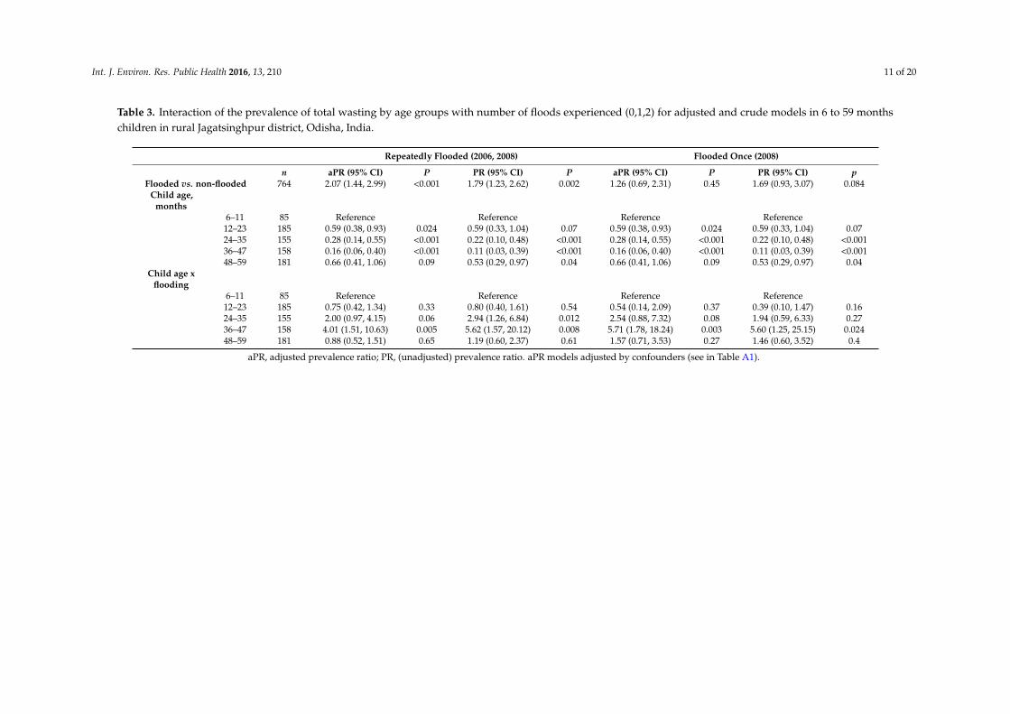
Int. J. Environ. Res. Public Health 2016, 13, 210 11 of 20
Table 3. Interaction of the prevalence of total wasting by age groups with number of floods experienced (0,1,2) for adjusted and crude models in 6 to 59 monthschildren in rural Jagatsinghpur district, Odisha, India.
Repeatedly Flooded (2006, 2008) Flooded Once (2008)
n aPR (95% CI) P PR (95% CI) P aPR (95% CI) P PR (95% CI) pFlooded vs. non-flooded 764 2.07 (1.44, 2.99) <0.001 1.79 (1.23, 2.62) 0.002 1.26 (0.69, 2.31) 0.45 1.69 (0.93, 3.07) 0.084
Child age,months
6–11 85 Reference Reference Reference Reference12–23 185 0.59 (0.38, 0.93) 0.024 0.59 (0.33, 1.04) 0.07 0.59 (0.38, 0.93) 0.024 0.59 (0.33, 1.04) 0.0724–35 155 0.28 (0.14, 0.55) <0.001 0.22 (0.10, 0.48) <0.001 0.28 (0.14, 0.55) <0.001 0.22 (0.10, 0.48) <0.00136–47 158 0.16 (0.06, 0.40) <0.001 0.11 (0.03, 0.39) <0.001 0.16 (0.06, 0.40) <0.001 0.11 (0.03, 0.39) <0.00148–59 181 0.66 (0.41, 1.06) 0.09 0.53 (0.29, 0.97) 0.04 0.66 (0.41, 1.06) 0.09 0.53 (0.29, 0.97) 0.04
Child age xflooding
6–11 85 Reference Reference Reference Reference12–23 185 0.75 (0.42, 1.34) 0.33 0.80 (0.40, 1.61) 0.54 0.54 (0.14, 2.09) 0.37 0.39 (0.10, 1.47) 0.1624–35 155 2.00 (0.97, 4.15) 0.06 2.94 (1.26, 6.84) 0.012 2.54 (0.88, 7.32) 0.08 1.94 (0.59, 6.33) 0.2736–47 158 4.01 (1.51, 10.63) 0.005 5.62 (1.57, 20.12) 0.008 5.71 (1.78, 18.24) 0.003 5.60 (1.25, 25.15) 0.02448–59 181 0.88 (0.52, 1.51) 0.65 1.19 (0.60, 2.37) 0.61 1.57 (0.71, 3.53) 0.27 1.46 (0.60, 3.52) 0.4
aPR, adjusted prevalence ratio; PR, (unadjusted) prevalence ratio. aPR models adjusted by confounders (see in Table A1).
Int. J. Environ. Res. Public Health 2016, 13, 210 12 of 20
Our findings show that in both exposure groups, communities flooded once or twice, theprevalence of child wasting was substantially increased (relative to those non-flooded). In contrast,being repeatedly exposed to floods proved to have additionally negative effects on these children. Thisstudy makes novel contributions to virtually unexplored aspects of the impacts on nutritional healthof the children living in flood prone rural areas. First, this evidence improves the understanding of therole of repeated flooding on children’s nutritional status, mainly by showing an increased likelihoodof severe wasting in recurrently flooded children. Second, we showed that the youngest children(0–12 months) are particularly vulnerable to the nutritional impacts of floods, which supports previousfindings from studies in India, Peru and Ecuador [7,34,35].
Overall, the available literature has pointed to growth failure as the dominant problem inpost-flood settings [6,7,34,36]. One study on 180 children after 1998 floods in rural Bangladeshfound reductions in the prevalence of wasting from the crisis period (17%) to the onset of theemergency response (12%) [37] but did not investigate the impacts on children’s health after fourmonths. In another study researching the same flood event in Bangladesh, Del Ninno and Lundberg [6]investigated 237 children in three waves up to 15 month post-flood but only found a worsening inheight-for-age, where effects were more severe and lasted longer in the youngest cohort (0–12 months),which is consistent with our findings. The same report however proposed that most children haverecovered by 15 months. This was not the case in Odisha by far. Whether weight-for-height orheight-for-age are more prevalent after flooding depend on the flood experience of the children’spopulation. Although a higher prevalence of weight-for-height often express a recent process of acuteweight loss, it can also reflects chronic unfavorable conditions [33], which was likely the case here.Typically, a rise in the prevalence of wasting might occur if food is suddenly not available. However,our results suggest that situations in which severe crop losses occur in vulnerable populations mightset chronic adverse conditions to access food in sufficient quantity. This food deprivation, combinedwith other factors, may contribute to weight losses among the affected children and eventually triggera protracted nutritional crisis [33].
In rural India, a previous community-based survey we conducted in the same study area showedthat the prevalence of child wasting one month after 2008 floods were 12.2% and 11.9%, respectivelyin flooded and non-flooded rural communities. This is additional evidence supporting that theobserved differences in the prevalence of wasting are due to the effect of flooding and not to baselinedifferences in child wasting among populations. In a previous study, growth failure proved to bethe dominant problem and was attributed to flooding approximately two years earlier, in August2006 [7]. One plausible explanation for the difference between indicators is the larger magnitude ofthe 2008 floods compared to those occurring in 2006, which was corroborated with survey householddata [7]. Supporting evidence on this aspect is the lower number of villages affected by floods in2006 compared to 2008 floods. The exceptional severity of the 2008 floods in our study area mighthave worsened the living conditions of these communities, with more manifest repercussions on thechildren’ nutritional status.
In this study, we found the highest prevalence of severe wasting in children exposed to repeatedflood, which showcases an important gap in current knowledge. Given that a nearly two-fold differencein the prevalence of severe wasting was observed in those communities repeatedly flooded relative tothose flooded in 2008 (aPR: 1.92; 95% CI: 0.95, 3.86), could repeated exposure to floods increase a child’ssusceptibility to severe forms of malnutrition? We did not find much evidence on if and how repeatedflooding can impact children’s physical health [5]. Some evidence suggest that the likelihood of mentalhealth problems in children affected by disasters (i.e., tsunamis) is also enhanced by previous traumaticexperiences, including exposure to war [38]. However, noting that the risk of death is substantiallyhigher in severely wasted children [39], more focused studies addressing this specific question areurgently needed.
This is the first study showing that flood events can produce protracted nutritional crises, even incommunities where floods are commonplace. Our study uses a sound epidemiological design, and
Int. J. Environ. Res. Public Health 2016, 13, 210 13 of 20
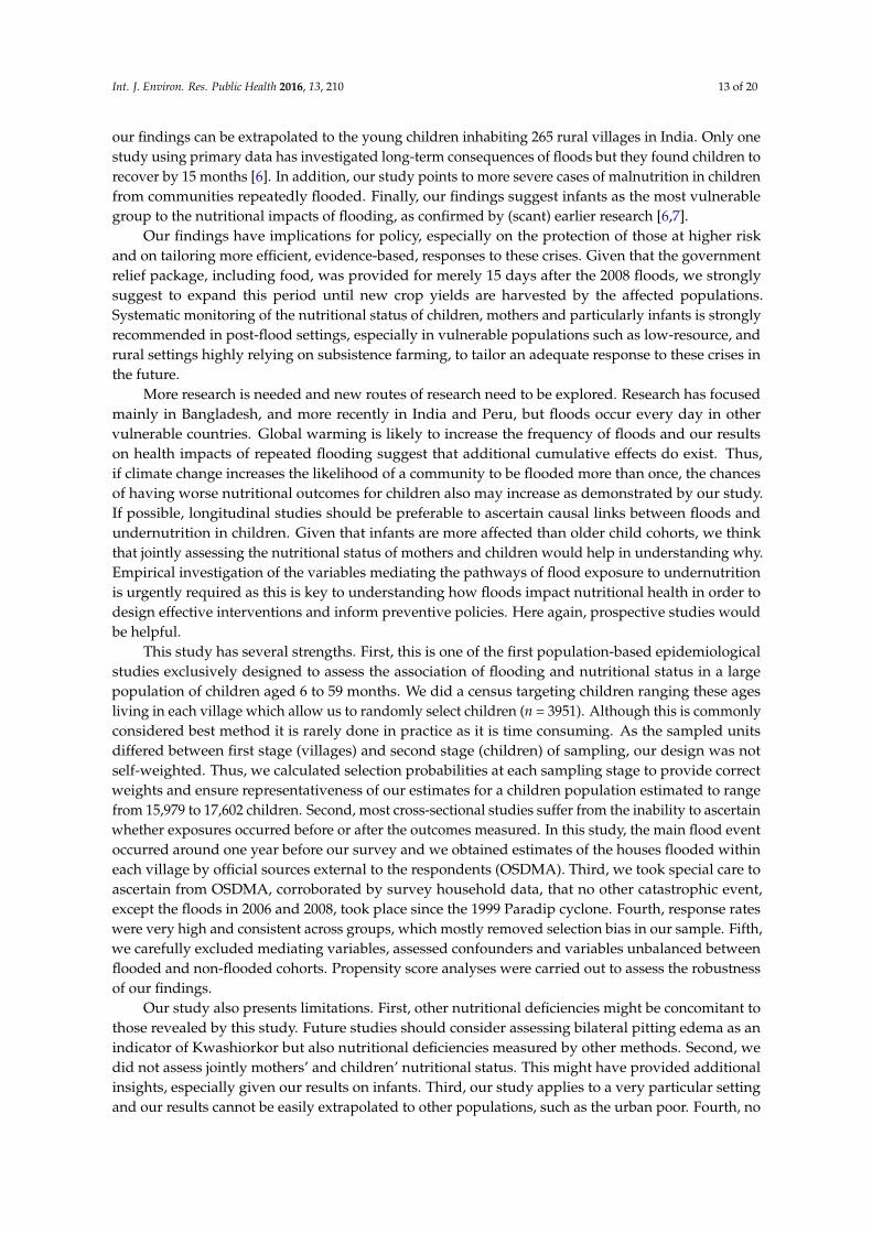
our findings can be extrapolated to the young children inhabiting 265 rural villages in India. Only onestudy using primary data has investigated long-term consequences of floods but they found children torecover by 15 months [6]. In addition, our study points to more severe cases of malnutrition in childrenfrom communities repeatedly flooded. Finally, our findings suggest infants as the most vulnerablegroup to the nutritional impacts of flooding, as confirmed by (scant) earlier research [6,7].
Our findings have implications for policy, especially on the protection of those at higher riskand on tailoring more efficient, evidence-based, responses to these crises. Given that the governmentrelief package, including food, was provided for merely 15 days after the 2008 floods, we stronglysuggest to expand this period until new crop yields are harvested by the affected populations.Systematic monitoring of the nutritional status of children, mothers and particularly infants is stronglyrecommended in post-flood settings, especially in vulnerable populations such as low-resource, andrural settings highly relying on subsistence farming, to tailor an adequate response to these crises inthe future.
More research is needed and new routes of research need to be explored. Research has focusedmainly in Bangladesh, and more recently in India and Peru, but floods occur every day in othervulnerable countries. Global warming is likely to increase the frequency of floods and our resultson health impacts of repeated flooding suggest that additional cumulative effects do exist. Thus,if climate change increases the likelihood of a community to be flooded more than once, the chancesof having worse nutritional outcomes for children also may increase as demonstrated by our study.If possible, longitudinal studies should be preferable to ascertain causal links between floods andundernutrition in children. Given that infants are more affected than older child cohorts, we thinkthat jointly assessing the nutritional status of mothers and children would help in understanding why.Empirical investigation of the variables mediating the pathways of flood exposure to undernutritionis urgently required as this is key to understanding how floods impact nutritional health in order todesign effective interventions and inform preventive policies. Here again, prospective studies wouldbe helpful.
This study has several strengths. First, this is one of the first population-based epidemiologicalstudies exclusively designed to assess the association of flooding and nutritional status in a largepopulation of children aged 6 to 59 months. We did a census targeting children ranging these agesliving in each village which allow us to randomly select children (n = 3951). Although this is commonlyconsidered best method it is rarely done in practice as it is time consuming. As the sampled unitsdiffered between first stage (villages) and second stage (children) of sampling, our design was notself-weighted. Thus, we calculated selection probabilities at each sampling stage to provide correctweights and ensure representativeness of our estimates for a children population estimated to rangefrom 15,979 to 17,602 children. Second, most cross-sectional studies suffer from the inability to ascertainwhether exposures occurred before or after the outcomes measured. In this study, the main flood eventoccurred around one year before our survey and we obtained estimates of the houses flooded withineach village by official sources external to the respondents (OSDMA). Third, we took special care toascertain from OSDMA, corroborated by survey household data, that no other catastrophic event,except the floods in 2006 and 2008, took place since the 1999 Paradip cyclone. Fourth, response rateswere very high and consistent across groups, which mostly removed selection bias in our sample. Fifth,we carefully excluded mediating variables, assessed confounders and variables unbalanced betweenflooded and non-flooded cohorts. Propensity score analyses were carried out to assess the robustnessof our findings.
Our study also presents limitations. First, other nutritional deficiencies might be concomitant tothose revealed by this study. Future studies should consider assessing bilateral pitting edema as anindicator of Kwashiorkor but also nutritional deficiencies measured by other methods. Second, wedid not assess jointly mothers’ and children’ nutritional status. This might have provided additionalinsights, especially given our results on infants. Third, our study applies to a very particular settingand our results cannot be easily extrapolated to other populations, such as the urban poor. Fourth, no

Int. J. Environ. Res. Public Health 2016, 13, 210 14 of 20
baseline but a comparison group was provided in this study and given its design a causal link is difficultto establish. However, the inclusion of children from nearby non-flooded villages likely contributed tocontrol for unobserved variables (see Figure A1). Fifth, out-migration could be a potential source ofbias if out-migrants are different from those who remain. However, we analyzed unpublished data ona survey conducted two years after the 2008 floods representing similar communities and found thatout-migration rates within households was very low in flood-affected areas (2.3%), and also relativeto non-flooded areas (1.0%). This is consistent with 15-year record showing modest migration afterflooding in Bangladesh [40].
5. Conclusions
In these Indian communities, flood-related undernutition persisted well beyond the typical periodof emergency relief. In our specific setting, wasting was more prominent than underweight or stuntingto indicate the nutritional stresses experienced by the affected child populations. In addition, wefound that not only is the burden of undernutrition greater among the flood-affected children andparticularly among infants, but the severity of this condition is significantly higher in repeatedlyflooded children. Global climate changes are set to increase flooding both in frequency and severitywhich will further aggravate this situation, particularly in low-resource settings or rural populationswhere susbsistence farming is very common [41]. In these contexts, we recommend the followingactions. Protracted nutritional response after floods should be seriously considered to counteract thelong-term nutritional effects on children. In areas where flooding is a recurrent occurrence, policies forrelief should be reviewed to ensure a longer period of support and proper take up by developmentprograms. Particularly attention should be paid to the nutritional health of mothers as the effects areworst amongst infants. Most importantly, preventive action should be put in place to protect mothersand children in flood prone areas. Systematic and long-lasting monitoring of the nutritional status ofvulnerable groups in the aftermath of floods (but also pre-flood if possible) might be helpful to tailorthe response and food supply in each particular context. Further stringent epidemiological studiesthat bring evidence on floods and nutrition to inform public health policies within the climate changeframework are urgently required.
Acknowledgments: We are grateful to Jean Macq, Niko Speybroeck, Sophie Vanwambeke and Philippe Donnenfor comments and guidance. We are thankful to Pascaline Wallemacq for preparing the map. This research wasfunded by the European FP6 6th Framework Programme under The MICRODIS Project—Integrated Health, Socialand Economic Impacts of Extreme Events: Evidence, Methods and Tools (Contract No GOCE-CT-2007-036877).
Author Contributions: Jose Manuel Rodriguez-Llanes, Shishir Ranjan-Dash and Debarati Guha-Sapir conceivedand designed the experiments; Shishir Ranjan-Dash and Alok Mukhopadhyay performed the experiments; JoseManuel Rodriguez-Llanes analyzed the data; Jose Manuel Rodriguez-Llanes and Shishir Ranjan-Dash contributedreagents/materials/analysis tools; Jose Manuel Rodriguez-Llanes wrote the paper.
Conflicts of Interest: The authors declare no conflict of interest. The founding sponsors had no role in the designof the study; in the collection, analyses, or interpretation of data; in the writing of the manuscript, and in thedecision to publish the results.
Abbreviations
The following abbreviations are used in this manuscript:
aPR adjusted prevalence ratioENA emergency nutrition assessmentICDS Integrated Child Development SchemeOSDMA Odisha state disaster mitigation authorityPR prevalence ratioPSU primary sampling unitSSU secondary sampling unitSMART standardized monitoring and assessment of relief and transitions
Int. J. Environ. Res. Public Health 2016, 13, 210 15 of 20
UNICEF United Nations children’s fund
Appendix A
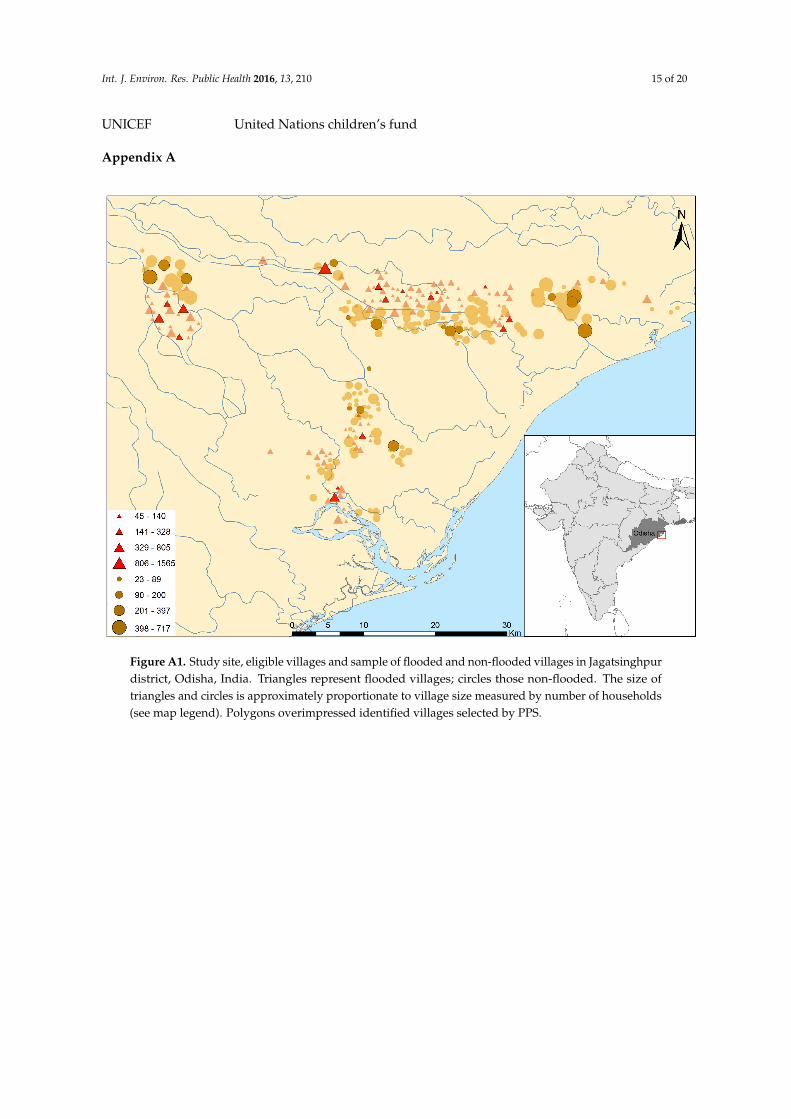
Figure A1. Study site, eligible villages and sample of flooded and non-flooded villages in Jagatsinghpurdistrict, Odisha, India. Triangles represent flooded villages; circles those non-flooded. The size oftriangles and circles is approximately proportionate to village size measured by number of households(see map legend). Polygons overimpressed identified villages selected by PPS.

Int. J. Environ. Res. Public Health 2016, 13, 210 16 of 20
Table A1. Overview of variables with frequencies differing across exposure and plausible confounders of undernutrition indicators in children of rural Jagatsinghpurdistrict, Odisha, India.
Flooded vs.Non-Flooded Confounders (p ď 0.2)
Variables Wasting Stunting UnderweightChild characteristics Moderate Severe Total Moderate Severe Total Moderate Severe Total
Child female NS No Yes Yes Yes No Yes No No NoMean birthweight, g NS Yes Yes Yes No Yes Yes No Yes YesChild age, months p ď 0.2 Yes Yes Yes Yes Yes Yes Yes Yes No
Underlying CausesCare of mother and children
Mean age at marriage of the mother, y p ď 0.2 No No No No No No Yes Yes YesMean age of the mother at first delivery, y p ď 0.2 Yes Yes Yes Yes No Yes No Yes NoMean age of the mother at birth of child, y NS Yes Yes No No No Yes Yes No YesMean age of the father at birth of child, y NS No Yes Yes Yes No No No Yes No
Two or more children underfive eating from same kitchen NS No No No No No No No No NoMother was a member of self-help group/Mahila Mandal NS Yes Yes No No No No No No No
Mean number of mother‘s conceptions NS Yes Yes No Yes No Yes Yes No YesMother had one or more miscarriages, stillbirths NS No No Yes Yes Yes Yes No No No
Child breastfed at least 2 years NS No No No No No No No Yes NoSupplementary feeding started after 6 months of child‘s age NS Yes Yes No No Yes Yes No Yes No
Child breastfed at least 2 years and supplemented after 6 months of age p ď 0.2 Yes No Yes No No No No No NoMother washes hands with soap before feeding child p ď 0.2 No No No No No No No No No
Mother washes hands with soap before preparing food for the family p ď 0.2 Yes No Yes No No No No No NoMother washes hands with soap before lunch NS No Yes Yes Yes Yes No No No No
Mother washes hands with soap after attending the child who defecated NS Yes No Yes Yes Yes Yes Yes No YesChild received BCG vaccine NS No Yes Yes No Yes No Yes Yes Yes
Child received measles vaccine NS No Yes No No Yes Yes No Yes YesChild received all three doses of polio vaccine NS Yes Yes Yes Yes No Yes No No No
Child received all three doses of B-hepatitis vaccine NS No Yes No No Yes No Yes No YesChild received all three doses of DPT vaccine NS Yes Yes No Yes Yes Yes Yes Yes No
Public healthImproved latrine (before floods) p ď 0.2 No No No No Yes No Yes No No
Improved drinking water (before floods) p ď 0.2 No No No No No No No Yes NoMother gave birth at hospital NS No No No No No No Yes No Yes
Number of individuals eating from same kitchen p ď 0.2 Yes Yes Yes Yes No Yes No Yes YesCapital
Household did borrow money (loan, credit, micro-credit) NS No No No Yes No Yes Yes Yes NoMaternal education p ď 0.2 Yes Yes Yes Yes Yes Yes No 1 Yes YesPaternal education p ď 0.2 Yes Yes Yes No Yes Yes Yes Yes Yes
Land ownership, hectare p ď 0.2 No Yes No Yes Yes Yes No Yes YesBasic causes
Religion NS Yes Yes Yes Yes Yes Yes Yes Yes YesCaste p ď 0.2 Yes Yes Yes Yes Yes Yes Yes Yes Yes
1 Model did not converge using mother education and this variable was excluded. NS, non-significant (i.e., p > 0.2).
Int. J. Environ. Res. Public Health 2016, 13, 210 17 of 20
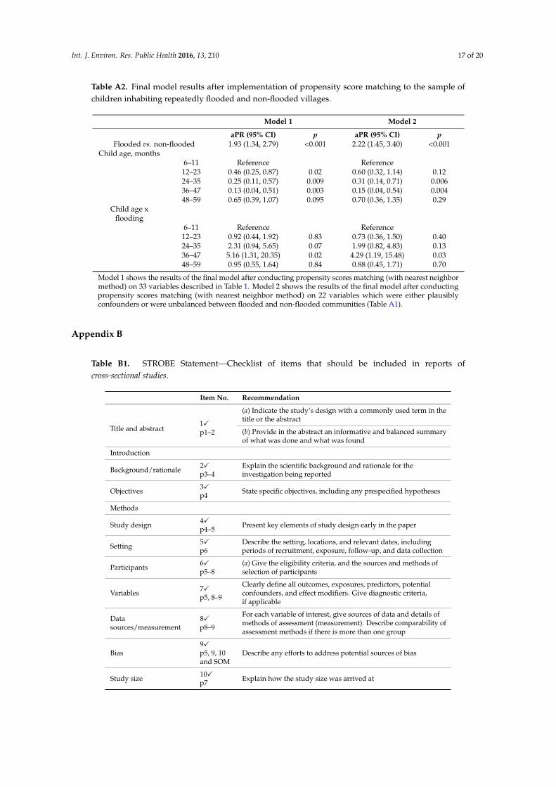
Table A2. Final model results after implementation of propensity score matching to the sample ofchildren inhabiting repeatedly flooded and non-flooded villages.
Model 1 Model 2
aPR (95% CI) p aPR (95% CI) pFlooded vs. non-flooded 1.93 (1.34, 2.79) <0.001 2.22 (1.45, 3.40) <0.001
Child age, months6–11 Reference Reference
12–23 0.46 (0.25, 0.87) 0.02 0.60 (0.32, 1.14) 0.1224–35 0.25 (0.11, 0.57) 0.009 0.31 (0.14, 0.71) 0.00636–47 0.13 (0.04, 0.51) 0.003 0.15 (0.04, 0.54) 0.00448–59 0.65 (0.39, 1.07) 0.095 0.70 (0.36, 1.35) 0.29
Child age xflooding
6–11 Reference Reference12–23 0.92 (0.44, 1.92) 0.83 0.73 (0.36, 1.50) 0.4024–35 2.31 (0.94, 5.65) 0.07 1.99 (0.82, 4.83) 0.1336–47 5.16 (1.31, 20.35) 0.02 4.29 (1.19, 15.48) 0.0348–59 0.95 (0.55, 1.64) 0.84 0.88 (0.45, 1.71) 0.70
Model 1 shows the results of the final model after conducting propensity scores matching (with nearest neighbormethod) on 33 variables described in Table 1. Model 2 shows the results of the final model after conductingpropensity scores matching (with nearest neighbor method) on 22 variables which were either plausiblyconfounders or were unbalanced between flooded and non-flooded communities (Table A1).
Appendix B
Table B1. STROBE Statement—Checklist of items that should be included in reports ofcross-sectional studies.
Item No. Recommendation
Title and abstract1
Int. J. Environ. Res. Public Health 2016, 13, 210 18 of 22
Table A2. Final model results after implementation of propensity score matching to the sample of children inhabiting repeatedly flooded and non-flooded villages.
Model 1 Model 2
aPR (95% CI) p aPR (95% CI) p
Flooded vs. non-flooded 1.93 (1.34, 2.79) <0.001 2.22 (1.45, 3.40) <0.001
Child age, months
6–11 Reference Reference
12–23 0.46 (0.25, 0.87) 0.02 0.60 (0.32, 1.14) 0.12
24–35 0.25 (0.11, 0.57) 0.009 0.31 (0.14, 0.71) 0.006
36–47 0.13 (0.04, 0.51) 0.003 0.15 (0.04, 0.54) 0.004
48–59 0.65 (0.39, 1.07) 0.095 0.70 (0.36, 1.35) 0.29
Child age x flooding
6–11 Reference Reference
12–23 0.92 (0.44, 1.92) 0.83 0.73 (0.36, 1.50) 0.40
24–35 2.31 (0.94, 5.65) 0.07 1.99 (0.82, 4.83) 0.13
36–47 5.16 (1.31, 20.35) 0.02 4.29 (1.19, 15.48) 0.03
48–59 0.95 (0.55, 1.64) 0.84 0.88 (0.45, 1.71) 0.70
Model 1 shows the results of the final model after conducting propensity scores matching (with nearest neighbor method) on 33 variables described in Table 1. Model 2 shows the results of the final model after conducting propensity scores matching (with nearest neighbor method) on 22 variables which were either plausibly confounders or were unbalanced between flooded and non-flooded communities (Table A1).
Appendix B
Table B1. STROBE Statement—Checklist of items that should be included in reports of cross-sectional studies.
Item No. Recommendation
Title and abstract 1 p1–2
(a) Indicate the study’s design with a commonly used term in the title or the abstract (b) Provide in the abstract an informative and balanced summary of what was done and what was found
Introduction
Background/rationale 2 p3–4
Explain the scientific background and rationale for the investigation being reported
Objectives 3 p4
State specific objectives, including any prespecified hypotheses
Methods
Study design 4 p4–5
Present key elements of study design early in the paper
Setting 5 p6
Describe the setting, locations, and relevant dates, including periods of recruitment, exposure, follow-up, and data collection
Participants 6 p5–8
(a) Give the eligibility criteria, and the sources and methods of selection of participants
p1–2
(a) Indicate the study’s design with a commonly used term in thetitle or the abstract
(b) Provide in the abstract an informative and balanced summaryof what was done and what was found
Introduction
Background/rationale 2
Int. J. Environ. Res. Public Health 2016, 13, 210 18 of 22
Table A2. Final model results after implementation of propensity score matching to the sample of children inhabiting repeatedly flooded and non-flooded villages.
Model 1 Model 2
aPR (95% CI) p aPR (95% CI) p
Flooded vs. non-flooded 1.93 (1.34, 2.79) <0.001 2.22 (1.45, 3.40) <0.001
Child age, months
6–11 Reference Reference
12–23 0.46 (0.25, 0.87) 0.02 0.60 (0.32, 1.14) 0.12
24–35 0.25 (0.11, 0.57) 0.009 0.31 (0.14, 0.71) 0.006
36–47 0.13 (0.04, 0.51) 0.003 0.15 (0.04, 0.54) 0.004
48–59 0.65 (0.39, 1.07) 0.095 0.70 (0.36, 1.35) 0.29
Child age x flooding
6–11 Reference Reference
12–23 0.92 (0.44, 1.92) 0.83 0.73 (0.36, 1.50) 0.40
24–35 2.31 (0.94, 5.65) 0.07 1.99 (0.82, 4.83) 0.13
36–47 5.16 (1.31, 20.35) 0.02 4.29 (1.19, 15.48) 0.03
48–59 0.95 (0.55, 1.64) 0.84 0.88 (0.45, 1.71) 0.70
Model 1 shows the results of the final model after conducting propensity scores matching (with nearest neighbor method) on 33 variables described in Table 1. Model 2 shows the results of the final model after conducting propensity scores matching (with nearest neighbor method) on 22 variables which were either plausibly confounders or were unbalanced between flooded and non-flooded communities (Table A1).
Appendix B
Table B1. STROBE Statement—Checklist of items that should be included in reports of cross-sectional studies.
Item No. Recommendation
Title and abstract 1 p1–2
(a) Indicate the study’s design with a commonly used term in the title or the abstract (b) Provide in the abstract an informative and balanced summary of what was done and what was found
Introduction
Background/rationale 2 p3–4
Explain the scientific background and rationale for the investigation being reported
Objectives 3 p4
State specific objectives, including any prespecified hypotheses
Methods
Study design 4 p4–5
Present key elements of study design early in the paper
Setting 5 p6
Describe the setting, locations, and relevant dates, including periods of recruitment, exposure, follow-up, and data collection
Participants 6 p5–8
(a) Give the eligibility criteria, and the sources and methods of selection of participants
p3–4Explain the scientific background and rationale for theinvestigation being reported
Objectives 3
Int. J. Environ. Res. Public Health 2016, 13, 210 18 of 22
Table A2. Final model results after implementation of propensity score matching to the sample of children inhabiting repeatedly flooded and non-flooded villages.
Model 1 Model 2
aPR (95% CI) p aPR (95% CI) p
Flooded vs. non-flooded 1.93 (1.34, 2.79) <0.001 2.22 (1.45, 3.40) <0.001
Child age, months
6–11 Reference Reference
12–23 0.46 (0.25, 0.87) 0.02 0.60 (0.32, 1.14) 0.12
24–35 0.25 (0.11, 0.57) 0.009 0.31 (0.14, 0.71) 0.006
36–47 0.13 (0.04, 0.51) 0.003 0.15 (0.04, 0.54) 0.004
48–59 0.65 (0.39, 1.07) 0.095 0.70 (0.36, 1.35) 0.29
Child age x flooding
6–11 Reference Reference
12–23 0.92 (0.44, 1.92) 0.83 0.73 (0.36, 1.50) 0.40
24–35 2.31 (0.94, 5.65) 0.07 1.99 (0.82, 4.83) 0.13
36–47 5.16 (1.31, 20.35) 0.02 4.29 (1.19, 15.48) 0.03
48–59 0.95 (0.55, 1.64) 0.84 0.88 (0.45, 1.71) 0.70
Model 1 shows the results of the final model after conducting propensity scores matching (with nearest neighbor method) on 33 variables described in Table 1. Model 2 shows the results of the final model after conducting propensity scores matching (with nearest neighbor method) on 22 variables which were either plausibly confounders or were unbalanced between flooded and non-flooded communities (Table A1).
Appendix B
Table B1. STROBE Statement—Checklist of items that should be included in reports of cross-sectional studies.
Item No. Recommendation
Title and abstract 1 p1–2
(a) Indicate the study’s design with a commonly used term in the title or the abstract (b) Provide in the abstract an informative and balanced summary of what was done and what was found
Introduction
Background/rationale 2 p3–4
Explain the scientific background and rationale for the investigation being reported
Objectives 3 p4
State specific objectives, including any prespecified hypotheses
Methods
Study design 4 p4–5
Present key elements of study design early in the paper
Setting 5 p6
Describe the setting, locations, and relevant dates, including periods of recruitment, exposure, follow-up, and data collection
Participants 6 p5–8
(a) Give the eligibility criteria, and the sources and methods of selection of participants
p4 State specific objectives, including any prespecified hypotheses
Methods
Study design 4
Int. J. Environ. Res. Public Health 2016, 13, 210 18 of 22
Table A2. Final model results after implementation of propensity score matching to the sample of children inhabiting repeatedly flooded and non-flooded villages.
Model 1 Model 2
aPR (95% CI) p aPR (95% CI) p
Flooded vs. non-flooded 1.93 (1.34, 2.79) <0.001 2.22 (1.45, 3.40) <0.001
Child age, months
6–11 Reference Reference
12–23 0.46 (0.25, 0.87) 0.02 0.60 (0.32, 1.14) 0.12
24–35 0.25 (0.11, 0.57) 0.009 0.31 (0.14, 0.71) 0.006
36–47 0.13 (0.04, 0.51) 0.003 0.15 (0.04, 0.54) 0.004
48–59 0.65 (0.39, 1.07) 0.095 0.70 (0.36, 1.35) 0.29
Child age x flooding
6–11 Reference Reference
12–23 0.92 (0.44, 1.92) 0.83 0.73 (0.36, 1.50) 0.40
24–35 2.31 (0.94, 5.65) 0.07 1.99 (0.82, 4.83) 0.13
36–47 5.16 (1.31, 20.35) 0.02 4.29 (1.19, 15.48) 0.03
48–59 0.95 (0.55, 1.64) 0.84 0.88 (0.45, 1.71) 0.70
Model 1 shows the results of the final model after conducting propensity scores matching (with nearest neighbor method) on 33 variables described in Table 1. Model 2 shows the results of the final model after conducting propensity scores matching (with nearest neighbor method) on 22 variables which were either plausibly confounders or were unbalanced between flooded and non-flooded communities (Table A1).
Appendix B
Table B1. STROBE Statement—Checklist of items that should be included in reports of cross-sectional studies.
Item No. Recommendation
Title and abstract 1 p1–2
(a) Indicate the study’s design with a commonly used term in the title or the abstract (b) Provide in the abstract an informative and balanced summary of what was done and what was found
Introduction
Background/rationale 2 p3–4
Explain the scientific background and rationale for the investigation being reported
Objectives 3 p4
State specific objectives, including any prespecified hypotheses
Methods
Study design 4 p4–5
Present key elements of study design early in the paper
Setting 5 p6
Describe the setting, locations, and relevant dates, including periods of recruitment, exposure, follow-up, and data collection
Participants 6 p5–8
(a) Give the eligibility criteria, and the sources and methods of selection of participants
p4–5 Present key elements of study design early in the paper
Setting 5
Int. J. Environ. Res. Public Health 2016, 13, 210 18 of 22
Table A2. Final model results after implementation of propensity score matching to the sample of children inhabiting repeatedly flooded and non-flooded villages.
Model 1 Model 2
aPR (95% CI) p aPR (95% CI) p
Flooded vs. non-flooded 1.93 (1.34, 2.79) <0.001 2.22 (1.45, 3.40) <0.001
Child age, months
6–11 Reference Reference
12–23 0.46 (0.25, 0.87) 0.02 0.60 (0.32, 1.14) 0.12
24–35 0.25 (0.11, 0.57) 0.009 0.31 (0.14, 0.71) 0.006
36–47 0.13 (0.04, 0.51) 0.003 0.15 (0.04, 0.54) 0.004
48–59 0.65 (0.39, 1.07) 0.095 0.70 (0.36, 1.35) 0.29
Child age x flooding
6–11 Reference Reference
12–23 0.92 (0.44, 1.92) 0.83 0.73 (0.36, 1.50) 0.40
24–35 2.31 (0.94, 5.65) 0.07 1.99 (0.82, 4.83) 0.13
36–47 5.16 (1.31, 20.35) 0.02 4.29 (1.19, 15.48) 0.03
48–59 0.95 (0.55, 1.64) 0.84 0.88 (0.45, 1.71) 0.70
Model 1 shows the results of the final model after conducting propensity scores matching (with nearest neighbor method) on 33 variables described in Table 1. Model 2 shows the results of the final model after conducting propensity scores matching (with nearest neighbor method) on 22 variables which were either plausibly confounders or were unbalanced between flooded and non-flooded communities (Table A1).
Appendix B
Table B1. STROBE Statement—Checklist of items that should be included in reports of cross-sectional studies.
Item No. Recommendation
Title and abstract 1 p1–2
(a) Indicate the study’s design with a commonly used term in the title or the abstract (b) Provide in the abstract an informative and balanced summary of what was done and what was found
Introduction
Background/rationale 2 p3–4
Explain the scientific background and rationale for the investigation being reported
Objectives 3 p4
State specific objectives, including any prespecified hypotheses
Methods
Study design 4 p4–5
Present key elements of study design early in the paper
Setting 5 p6
Describe the setting, locations, and relevant dates, including periods of recruitment, exposure, follow-up, and data collection
Participants 6 p5–8
(a) Give the eligibility criteria, and the sources and methods of selection of participants
p6Describe the setting, locations, and relevant dates, includingperiods of recruitment, exposure, follow-up, and data collection
Participants 6
Int. J. Environ. Res. Public Health 2016, 13, 210 18 of 22
Table A2. Final model results after implementation of propensity score matching to the sample of children inhabiting repeatedly flooded and non-flooded villages.
Model 1 Model 2
aPR (95% CI) p aPR (95% CI) p
Flooded vs. non-flooded 1.93 (1.34, 2.79) <0.001 2.22 (1.45, 3.40) <0.001
Child age, months
6–11 Reference Reference
12–23 0.46 (0.25, 0.87) 0.02 0.60 (0.32, 1.14) 0.12
24–35 0.25 (0.11, 0.57) 0.009 0.31 (0.14, 0.71) 0.006
36–47 0.13 (0.04, 0.51) 0.003 0.15 (0.04, 0.54) 0.004
48–59 0.65 (0.39, 1.07) 0.095 0.70 (0.36, 1.35) 0.29
Child age x flooding
6–11 Reference Reference
12–23 0.92 (0.44, 1.92) 0.83 0.73 (0.36, 1.50) 0.40
24–35 2.31 (0.94, 5.65) 0.07 1.99 (0.82, 4.83) 0.13
36–47 5.16 (1.31, 20.35) 0.02 4.29 (1.19, 15.48) 0.03
48–59 0.95 (0.55, 1.64) 0.84 0.88 (0.45, 1.71) 0.70
Model 1 shows the results of the final model after conducting propensity scores matching (with nearest neighbor method) on 33 variables described in Table 1. Model 2 shows the results of the final model after conducting propensity scores matching (with nearest neighbor method) on 22 variables which were either plausibly confounders or were unbalanced between flooded and non-flooded communities (Table A1).
Appendix B
Table B1. STROBE Statement—Checklist of items that should be included in reports of cross-sectional studies.
Item No. Recommendation
Title and abstract 1 p1–2
(a) Indicate the study’s design with a commonly used term in the title or the abstract (b) Provide in the abstract an informative and balanced summary of what was done and what was found
Introduction
Background/rationale 2 p3–4
Explain the scientific background and rationale for the investigation being reported
Objectives 3 p4
State specific objectives, including any prespecified hypotheses
Methods
Study design 4 p4–5
Present key elements of study design early in the paper
Setting 5 p6
Describe the setting, locations, and relevant dates, including periods of recruitment, exposure, follow-up, and data collection
Participants 6 p5–8
(a) Give the eligibility criteria, and the sources and methods of selection of participants
p5–8(a) Give the eligibility criteria, and the sources and methods ofselection of participants
Variables 7
Int. J. Environ. Res. Public Health 2016, 13, 210 18 of 22
Table A2. Final model results after implementation of propensity score matching to the sample of children inhabiting repeatedly flooded and non-flooded villages.
Model 1 Model 2
aPR (95% CI) p aPR (95% CI) p
Flooded vs. non-flooded 1.93 (1.34, 2.79) <0.001 2.22 (1.45, 3.40) <0.001
Child age, months
6–11 Reference Reference
12–23 0.46 (0.25, 0.87) 0.02 0.60 (0.32, 1.14) 0.12
24–35 0.25 (0.11, 0.57) 0.009 0.31 (0.14, 0.71) 0.006
36–47 0.13 (0.04, 0.51) 0.003 0.15 (0.04, 0.54) 0.004
48–59 0.65 (0.39, 1.07) 0.095 0.70 (0.36, 1.35) 0.29
Child age x flooding
6–11 Reference Reference
12–23 0.92 (0.44, 1.92) 0.83 0.73 (0.36, 1.50) 0.40
24–35 2.31 (0.94, 5.65) 0.07 1.99 (0.82, 4.83) 0.13
36–47 5.16 (1.31, 20.35) 0.02 4.29 (1.19, 15.48) 0.03
48–59 0.95 (0.55, 1.64) 0.84 0.88 (0.45, 1.71) 0.70
Model 1 shows the results of the final model after conducting propensity scores matching (with nearest neighbor method) on 33 variables described in Table 1. Model 2 shows the results of the final model after conducting propensity scores matching (with nearest neighbor method) on 22 variables which were either plausibly confounders or were unbalanced between flooded and non-flooded communities (Table A1).
Appendix B
Table B1. STROBE Statement—Checklist of items that should be included in reports of cross-sectional studies.
Item No. Recommendation
Title and abstract 1 p1–2
(a) Indicate the study’s design with a commonly used term in the title or the abstract (b) Provide in the abstract an informative and balanced summary of what was done and what was found
Introduction
Background/rationale 2 p3–4
Explain the scientific background and rationale for the investigation being reported
Objectives 3 p4
State specific objectives, including any prespecified hypotheses
Methods
Study design 4 p4–5
Present key elements of study design early in the paper
Setting 5 p6
Describe the setting, locations, and relevant dates, including periods of recruitment, exposure, follow-up, and data collection
Participants 6 p5–8
(a) Give the eligibility criteria, and the sources and methods of selection of participants
p5, 8–9
Clearly define all outcomes, exposures, predictors, potentialconfounders, and effect modifiers. Give diagnostic criteria,if applicable
Datasources/measurement
8
Int. J. Environ. Res. Public Health 2016, 13, 210 18 of 22
Table A2. Final model results after implementation of propensity score matching to the sample of children inhabiting repeatedly flooded and non-flooded villages.
Model 1 Model 2
aPR (95% CI) p aPR (95% CI) p
Flooded vs. non-flooded 1.93 (1.34, 2.79) <0.001 2.22 (1.45, 3.40) <0.001
Child age, months
6–11 Reference Reference
12–23 0.46 (0.25, 0.87) 0.02 0.60 (0.32, 1.14) 0.12
24–35 0.25 (0.11, 0.57) 0.009 0.31 (0.14, 0.71) 0.006
36–47 0.13 (0.04, 0.51) 0.003 0.15 (0.04, 0.54) 0.004
48–59 0.65 (0.39, 1.07) 0.095 0.70 (0.36, 1.35) 0.29
Child age x flooding
6–11 Reference Reference
12–23 0.92 (0.44, 1.92) 0.83 0.73 (0.36, 1.50) 0.40
24–35 2.31 (0.94, 5.65) 0.07 1.99 (0.82, 4.83) 0.13
36–47 5.16 (1.31, 20.35) 0.02 4.29 (1.19, 15.48) 0.03
48–59 0.95 (0.55, 1.64) 0.84 0.88 (0.45, 1.71) 0.70
Model 1 shows the results of the final model after conducting propensity scores matching (with nearest neighbor method) on 33 variables described in Table 1. Model 2 shows the results of the final model after conducting propensity scores matching (with nearest neighbor method) on 22 variables which were either plausibly confounders or were unbalanced between flooded and non-flooded communities (Table A1).
Appendix B
Table B1. STROBE Statement—Checklist of items that should be included in reports of cross-sectional studies.
Item No. Recommendation
Title and abstract 1 p1–2
(a) Indicate the study’s design with a commonly used term in the title or the abstract (b) Provide in the abstract an informative and balanced summary of what was done and what was found
Introduction
Background/rationale 2 p3–4
Explain the scientific background and rationale for the investigation being reported
Objectives 3 p4
State specific objectives, including any prespecified hypotheses
Methods
Study design 4 p4–5
Present key elements of study design early in the paper
Setting 5 p6
Describe the setting, locations, and relevant dates, including periods of recruitment, exposure, follow-up, and data collection
Participants 6 p5–8
(a) Give the eligibility criteria, and the sources and methods of selection of participants
p8–9
For each variable of interest, give sources of data and details ofmethods of assessment (measurement). Describe comparability ofassessment methods if there is more than one group
Bias9
Int. J. Environ. Res. Public Health 2016, 13, 210 18 of 22
Table A2. Final model results after implementation of propensity score matching to the sample of children inhabiting repeatedly flooded and non-flooded villages.
Model 1 Model 2
aPR (95% CI) p aPR (95% CI) p
Flooded vs. non-flooded 1.93 (1.34, 2.79) <0.001 2.22 (1.45, 3.40) <0.001
Child age, months
6–11 Reference Reference
12–23 0.46 (0.25, 0.87) 0.02 0.60 (0.32, 1.14) 0.12
24–35 0.25 (0.11, 0.57) 0.009 0.31 (0.14, 0.71) 0.006
36–47 0.13 (0.04, 0.51) 0.003 0.15 (0.04, 0.54) 0.004
48–59 0.65 (0.39, 1.07) 0.095 0.70 (0.36, 1.35) 0.29
Child age x flooding
6–11 Reference Reference
12–23 0.92 (0.44, 1.92) 0.83 0.73 (0.36, 1.50) 0.40
24–35 2.31 (0.94, 5.65) 0.07 1.99 (0.82, 4.83) 0.13
36–47 5.16 (1.31, 20.35) 0.02 4.29 (1.19, 15.48) 0.03
48–59 0.95 (0.55, 1.64) 0.84 0.88 (0.45, 1.71) 0.70
Model 1 shows the results of the final model after conducting propensity scores matching (with nearest neighbor method) on 33 variables described in Table 1. Model 2 shows the results of the final model after conducting propensity scores matching (with nearest neighbor method) on 22 variables which were either plausibly confounders or were unbalanced between flooded and non-flooded communities (Table A1).
Appendix B
Table B1. STROBE Statement—Checklist of items that should be included in reports of cross-sectional studies.
Item No. Recommendation
Title and abstract 1 p1–2
(a) Indicate the study’s design with a commonly used term in the title or the abstract (b) Provide in the abstract an informative and balanced summary of what was done and what was found
Introduction
Background/rationale 2 p3–4
Explain the scientific background and rationale for the investigation being reported
Objectives 3 p4
State specific objectives, including any prespecified hypotheses
Methods
Study design 4 p4–5
Present key elements of study design early in the paper
Setting 5 p6
Describe the setting, locations, and relevant dates, including periods of recruitment, exposure, follow-up, and data collection
Participants 6 p5–8
(a) Give the eligibility criteria, and the sources and methods of selection of participants
p5, 9, 10and SOM
Describe any efforts to address potential sources of bias
Study size 10
Int. J. Environ. Res. Public Health 2016, 13, 210 18 of 22
Table A2. Final model results after implementation of propensity score matching to the sample of children inhabiting repeatedly flooded and non-flooded villages.
Model 1 Model 2
aPR (95% CI) p aPR (95% CI) p
Flooded vs. non-flooded 1.93 (1.34, 2.79) <0.001 2.22 (1.45, 3.40) <0.001
Child age, months
6–11 Reference Reference
12–23 0.46 (0.25, 0.87) 0.02 0.60 (0.32, 1.14) 0.12
24–35 0.25 (0.11, 0.57) 0.009 0.31 (0.14, 0.71) 0.006
36–47 0.13 (0.04, 0.51) 0.003 0.15 (0.04, 0.54) 0.004
48–59 0.65 (0.39, 1.07) 0.095 0.70 (0.36, 1.35) 0.29
Child age x flooding
6–11 Reference Reference
12–23 0.92 (0.44, 1.92) 0.83 0.73 (0.36, 1.50) 0.40
24–35 2.31 (0.94, 5.65) 0.07 1.99 (0.82, 4.83) 0.13
36–47 5.16 (1.31, 20.35) 0.02 4.29 (1.19, 15.48) 0.03
48–59 0.95 (0.55, 1.64) 0.84 0.88 (0.45, 1.71) 0.70
Model 1 shows the results of the final model after conducting propensity scores matching (with nearest neighbor method) on 33 variables described in Table 1. Model 2 shows the results of the final model after conducting propensity scores matching (with nearest neighbor method) on 22 variables which were either plausibly confounders or were unbalanced between flooded and non-flooded communities (Table A1).
Appendix B
Table B1. STROBE Statement—Checklist of items that should be included in reports of cross-sectional studies.
Item No. Recommendation
Title and abstract 1 p1–2
(a) Indicate the study’s design with a commonly used term in the title or the abstract (b) Provide in the abstract an informative and balanced summary of what was done and what was found
Introduction
Background/rationale 2 p3–4
Explain the scientific background and rationale for the investigation being reported
Objectives 3 p4
State specific objectives, including any prespecified hypotheses
Methods
Study design 4 p4–5
Present key elements of study design early in the paper
Setting 5 p6
Describe the setting, locations, and relevant dates, including periods of recruitment, exposure, follow-up, and data collection
Participants 6 p5–8
(a) Give the eligibility criteria, and the sources and methods of selection of participants
p7 Explain how the study size was arrived at

Int. J. Environ. Res. Public Health 2016, 13, 210 18 of 20
Table B1. Cont.
Item No. Recommendation
Quantitative variables 11
Int. J. Environ. Res. Public Health 2016, 13, 210 18 of 22
Table A2. Final model results after implementation of propensity score matching to the sample of children inhabiting repeatedly flooded and non-flooded villages.
Model 1 Model 2
aPR (95% CI) p aPR (95% CI) p
Flooded vs. non-flooded 1.93 (1.34, 2.79) <0.001 2.22 (1.45, 3.40) <0.001
Child age, months
6–11 Reference Reference
12–23 0.46 (0.25, 0.87) 0.02 0.60 (0.32, 1.14) 0.12
24–35 0.25 (0.11, 0.57) 0.009 0.31 (0.14, 0.71) 0.006
36–47 0.13 (0.04, 0.51) 0.003 0.15 (0.04, 0.54) 0.004
48–59 0.65 (0.39, 1.07) 0.095 0.70 (0.36, 1.35) 0.29
Child age x flooding
6–11 Reference Reference
12–23 0.92 (0.44, 1.92) 0.83 0.73 (0.36, 1.50) 0.40
24–35 2.31 (0.94, 5.65) 0.07 1.99 (0.82, 4.83) 0.13
36–47 5.16 (1.31, 20.35) 0.02 4.29 (1.19, 15.48) 0.03
48–59 0.95 (0.55, 1.64) 0.84 0.88 (0.45, 1.71) 0.70
Model 1 shows the results of the final model after conducting propensity scores matching (with nearest neighbor method) on 33 variables described in Table 1. Model 2 shows the results of the final model after conducting propensity scores matching (with nearest neighbor method) on 22 variables which were either plausibly confounders or were unbalanced between flooded and non-flooded communities (Table A1).
Appendix B
Table B1. STROBE Statement—Checklist of items that should be included in reports of cross-sectional studies.
Item No. Recommendation
Title and abstract 1 p1–2
(a) Indicate the study’s design with a commonly used term in the title or the abstract (b) Provide in the abstract an informative and balanced summary of what was done and what was found
Introduction
Background/rationale 2 p3–4
Explain the scientific background and rationale for the investigation being reported
Objectives 3 p4
State specific objectives, including any prespecified hypotheses
Methods
Study design 4 p4–5
Present key elements of study design early in the paper
Setting 5 p6
Describe the setting, locations, and relevant dates, including periods of recruitment, exposure, follow-up, and data collection
Participants 6 p5–8
(a) Give the eligibility criteria, and the sources and methods of selection of participants
p5, 8 and tablesExplain how quantitative variables were handled in the analyses.If applicable, describe which groupings were chosen and why
Statistical methods12
Int. J. Environ. Res. Public Health 2016, 13, 210 18 of 22
Table A2. Final model results after implementation of propensity score matching to the sample of children inhabiting repeatedly flooded and non-flooded villages.
Model 1 Model 2
aPR (95% CI) p aPR (95% CI) p
Flooded vs. non-flooded 1.93 (1.34, 2.79) <0.001 2.22 (1.45, 3.40) <0.001
Child age, months
6–11 Reference Reference
12–23 0.46 (0.25, 0.87) 0.02 0.60 (0.32, 1.14) 0.12
24–35 0.25 (0.11, 0.57) 0.009 0.31 (0.14, 0.71) 0.006
36–47 0.13 (0.04, 0.51) 0.003 0.15 (0.04, 0.54) 0.004
48–59 0.65 (0.39, 1.07) 0.095 0.70 (0.36, 1.35) 0.29
Child age x flooding
6–11 Reference Reference
12–23 0.92 (0.44, 1.92) 0.83 0.73 (0.36, 1.50) 0.40
24–35 2.31 (0.94, 5.65) 0.07 1.99 (0.82, 4.83) 0.13
36–47 5.16 (1.31, 20.35) 0.02 4.29 (1.19, 15.48) 0.03
48–59 0.95 (0.55, 1.64) 0.84 0.88 (0.45, 1.71) 0.70
Model 1 shows the results of the final model after conducting propensity scores matching (with nearest neighbor method) on 33 variables described in Table 1. Model 2 shows the results of the final model after conducting propensity scores matching (with nearest neighbor method) on 22 variables which were either plausibly confounders or were unbalanced between flooded and non-flooded communities (Table A1).
Appendix B
Table B1. STROBE Statement—Checklist of items that should be included in reports of cross-sectional studies.
Item No. Recommendation
Title and abstract 1 p1–2
(a) Indicate the study’s design with a commonly used term in the title or the abstract (b) Provide in the abstract an informative and balanced summary of what was done and what was found
Introduction
Background/rationale 2 p3–4
Explain the scientific background and rationale for the investigation being reported
Objectives 3 p4
State specific objectives, including any prespecified hypotheses
Methods
Study design 4 p4–5
Present key elements of study design early in the paper
Setting 5 p6
Describe the setting, locations, and relevant dates, including periods of recruitment, exposure, follow-up, and data collection
Participants 6 p5–8
(a) Give the eligibility criteria, and the sources and methods of selection of participants
p9–10
(a) Describe all statistical methods, including those used to controlfor confounding
(b) Describe any methods used to examine subgroups and interactions
(c) Explain how missing data were addressed
(d) If applicable, describe analytical methods taking account ofsampling strategy
(e) Describe any sensitivity analyses
Results
Participants 13
Int. J. Environ. Res. Public Health 2016, 13, 210 18 of 22
Table A2. Final model results after implementation of propensity score matching to the sample of children inhabiting repeatedly flooded and non-flooded villages.
Model 1 Model 2
aPR (95% CI) p aPR (95% CI) p
Flooded vs. non-flooded 1.93 (1.34, 2.79) <0.001 2.22 (1.45, 3.40) <0.001
Child age, months
6–11 Reference Reference
12–23 0.46 (0.25, 0.87) 0.02 0.60 (0.32, 1.14) 0.12
24–35 0.25 (0.11, 0.57) 0.009 0.31 (0.14, 0.71) 0.006
36–47 0.13 (0.04, 0.51) 0.003 0.15 (0.04, 0.54) 0.004
48–59 0.65 (0.39, 1.07) 0.095 0.70 (0.36, 1.35) 0.29
Child age x flooding
6–11 Reference Reference
12–23 0.92 (0.44, 1.92) 0.83 0.73 (0.36, 1.50) 0.40
24–35 2.31 (0.94, 5.65) 0.07 1.99 (0.82, 4.83) 0.13
36–47 5.16 (1.31, 20.35) 0.02 4.29 (1.19, 15.48) 0.03
48–59 0.95 (0.55, 1.64) 0.84 0.88 (0.45, 1.71) 0.70
Model 1 shows the results of the final model after conducting propensity scores matching (with nearest neighbor method) on 33 variables described in Table 1. Model 2 shows the results of the final model after conducting propensity scores matching (with nearest neighbor method) on 22 variables which were either plausibly confounders or were unbalanced between flooded and non-flooded communities (Table A1).
Appendix B
Table B1. STROBE Statement—Checklist of items that should be included in reports of cross-sectional studies.
Item No. Recommendation
Title and abstract 1 p1–2
(a) Indicate the study’s design with a commonly used term in the title or the abstract (b) Provide in the abstract an informative and balanced summary of what was done and what was found
Introduction
Background/rationale 2 p3–4
Explain the scientific background and rationale for the investigation being reported
Objectives 3 p4
State specific objectives, including any prespecified hypotheses
Methods
Study design 4 p4–5
Present key elements of study design early in the paper
Setting 5 p6
Describe the setting, locations, and relevant dates, including periods of recruitment, exposure, follow-up, and data collection
Participants 6 p5–8
(a) Give the eligibility criteria, and the sources and methods of selection of participants
p10
(a) Report numbers of individuals at each stage of study—e.g.,numbers potentially eligible, examined for eligibility, confirmedeligible, included in the study, completing follow-up, and analysed
(b) Give reasons for non-participation at each stage
Int. J. Environ. Res. Public Health 2016, 13, 210 18 of 22
Table A2. Final model results after implementation of propensity score matching to the sample of children inhabiting repeatedly flooded and non-flooded villages.
Model 1 Model 2
aPR (95% CI) p aPR (95% CI) p
Flooded vs. non-flooded 1.93 (1.34, 2.79) <0.001 2.22 (1.45, 3.40) <0.001
Child age, months
6–11 Reference Reference
12–23 0.46 (0.25, 0.87) 0.02 0.60 (0.32, 1.14) 0.12
24–35 0.25 (0.11, 0.57) 0.009 0.31 (0.14, 0.71) 0.006
36–47 0.13 (0.04, 0.51) 0.003 0.15 (0.04, 0.54) 0.004
48–59 0.65 (0.39, 1.07) 0.095 0.70 (0.36, 1.35) 0.29
Child age x flooding
6–11 Reference Reference
12–23 0.92 (0.44, 1.92) 0.83 0.73 (0.36, 1.50) 0.40
24–35 2.31 (0.94, 5.65) 0.07 1.99 (0.82, 4.83) 0.13
36–47 5.16 (1.31, 20.35) 0.02 4.29 (1.19, 15.48) 0.03
48–59 0.95 (0.55, 1.64) 0.84 0.88 (0.45, 1.71) 0.70
Model 1 shows the results of the final model after conducting propensity scores matching (with nearest neighbor method) on 33 variables described in Table 1. Model 2 shows the results of the final model after conducting propensity scores matching (with nearest neighbor method) on 22 variables which were either plausibly confounders or were unbalanced between flooded and non-flooded communities (Table A1).
Appendix B
Table B1. STROBE Statement—Checklist of items that should be included in reports of cross-sectional studies.
Item No. Recommendation
Title and abstract 1 p1–2
(a) Indicate the study’s design with a commonly used term in the title or the abstract (b) Provide in the abstract an informative and balanced summary of what was done and what was found
Introduction
Background/rationale 2 p3–4
Explain the scientific background and rationale for the investigation being reported
Objectives 3 p4
State specific objectives, including any prespecified hypotheses
Methods
Study design 4 p4–5
Present key elements of study design early in the paper
Setting 5 p6
Describe the setting, locations, and relevant dates, including periods of recruitment, exposure, follow-up, and data collection
Participants 6 p5–8
(a) Give the eligibility criteria, and the sources and methods of selection of participants
Figure 1
(c) Consider use of a flow diagram
Int. J. Environ. Res. Public Health 2016, 13, 210 18 of 22
Table A2. Final model results after implementation of propensity score matching to the sample of children inhabiting repeatedly flooded and non-flooded villages.
Model 1 Model 2
aPR (95% CI) p aPR (95% CI) p
Flooded vs. non-flooded 1.93 (1.34, 2.79) <0.001 2.22 (1.45, 3.40) <0.001
Child age, months
6–11 Reference Reference
12–23 0.46 (0.25, 0.87) 0.02 0.60 (0.32, 1.14) 0.12
24–35 0.25 (0.11, 0.57) 0.009 0.31 (0.14, 0.71) 0.006
36–47 0.13 (0.04, 0.51) 0.003 0.15 (0.04, 0.54) 0.004
48–59 0.65 (0.39, 1.07) 0.095 0.70 (0.36, 1.35) 0.29
Child age x flooding
6–11 Reference Reference
12–23 0.92 (0.44, 1.92) 0.83 0.73 (0.36, 1.50) 0.40
24–35 2.31 (0.94, 5.65) 0.07 1.99 (0.82, 4.83) 0.13
36–47 5.16 (1.31, 20.35) 0.02 4.29 (1.19, 15.48) 0.03
48–59 0.95 (0.55, 1.64) 0.84 0.88 (0.45, 1.71) 0.70
Model 1 shows the results of the final model after conducting propensity scores matching (with nearest neighbor method) on 33 variables described in Table 1. Model 2 shows the results of the final model after conducting propensity scores matching (with nearest neighbor method) on 22 variables which were either plausibly confounders or were unbalanced between flooded and non-flooded communities (Table A1).
Appendix B
Table B1. STROBE Statement—Checklist of items that should be included in reports of cross-sectional studies.
Item No. Recommendation
Title and abstract 1 p1–2
(a) Indicate the study’s design with a commonly used term in the title or the abstract (b) Provide in the abstract an informative and balanced summary of what was done and what was found
Introduction
Background/rationale 2 p3–4
Explain the scientific background and rationale for the investigation being reported
Objectives 3 p4
State specific objectives, including any prespecified hypotheses
Methods
Study design 4 p4–5
Present key elements of study design early in the paper
Setting 5 p6
Describe the setting, locations, and relevant dates, including periods of recruitment, exposure, follow-up, and data collection
Participants 6 p5–8
(a) Give the eligibility criteria, and the sources and methods of selection of participants
Figure 1
Descriptive data 14
Int. J. Environ. Res. Public Health 2016, 13, 210 18 of 22
Table A2. Final model results after implementation of propensity score matching to the sample of children inhabiting repeatedly flooded and non-flooded villages.
Model 1 Model 2
aPR (95% CI) p aPR (95% CI) p
Flooded vs. non-flooded 1.93 (1.34, 2.79) <0.001 2.22 (1.45, 3.40) <0.001
Child age, months
6–11 Reference Reference
12–23 0.46 (0.25, 0.87) 0.02 0.60 (0.32, 1.14) 0.12
24–35 0.25 (0.11, 0.57) 0.009 0.31 (0.14, 0.71) 0.006
36–47 0.13 (0.04, 0.51) 0.003 0.15 (0.04, 0.54) 0.004
48–59 0.65 (0.39, 1.07) 0.095 0.70 (0.36, 1.35) 0.29
Child age x flooding
6–11 Reference Reference
12–23 0.92 (0.44, 1.92) 0.83 0.73 (0.36, 1.50) 0.40
24–35 2.31 (0.94, 5.65) 0.07 1.99 (0.82, 4.83) 0.13
36–47 5.16 (1.31, 20.35) 0.02 4.29 (1.19, 15.48) 0.03
48–59 0.95 (0.55, 1.64) 0.84 0.88 (0.45, 1.71) 0.70
Model 1 shows the results of the final model after conducting propensity scores matching (with nearest neighbor method) on 33 variables described in Table 1. Model 2 shows the results of the final model after conducting propensity scores matching (with nearest neighbor method) on 22 variables which were either plausibly confounders or were unbalanced between flooded and non-flooded communities (Table A1).
Appendix B
Table B1. STROBE Statement—Checklist of items that should be included in reports of cross-sectional studies.
Item No. Recommendation
Title and abstract 1 p1–2
(a) Indicate the study’s design with a commonly used term in the title or the abstract (b) Provide in the abstract an informative and balanced summary of what was done and what was found
Introduction
Background/rationale 2 p3–4
Explain the scientific background and rationale for the investigation being reported
Objectives 3 p4
State specific objectives, including any prespecified hypotheses
Methods
Study design 4 p4–5
Present key elements of study design early in the paper
Setting 5 p6
Describe the setting, locations, and relevant dates, including periods of recruitment, exposure, follow-up, and data collection
Participants 6 p5–8
(a) Give the eligibility criteria, and the sources and methods of selection of participants
p10, table 1
(a) Give characteristics of study participants (e.g., demographic, clinical,social) and information on exposures and potential confounders
(b) Indicate number of participants with missing data for each variableof interest
Outcome data 15
Int. J. Environ. Res. Public Health 2016, 13, 210 18 of 22
Table A2. Final model results after implementation of propensity score matching to the sample of children inhabiting repeatedly flooded and non-flooded villages.
Model 1 Model 2
aPR (95% CI) p aPR (95% CI) p
Flooded vs. non-flooded 1.93 (1.34, 2.79) <0.001 2.22 (1.45, 3.40) <0.001
Child age, months
6–11 Reference Reference
12–23 0.46 (0.25, 0.87) 0.02 0.60 (0.32, 1.14) 0.12
24–35 0.25 (0.11, 0.57) 0.009 0.31 (0.14, 0.71) 0.006
36–47 0.13 (0.04, 0.51) 0.003 0.15 (0.04, 0.54) 0.004
48–59 0.65 (0.39, 1.07) 0.095 0.70 (0.36, 1.35) 0.29
Child age x flooding
6–11 Reference Reference
12–23 0.92 (0.44, 1.92) 0.83 0.73 (0.36, 1.50) 0.40
24–35 2.31 (0.94, 5.65) 0.07 1.99 (0.82, 4.83) 0.13
36–47 5.16 (1.31, 20.35) 0.02 4.29 (1.19, 15.48) 0.03
48–59 0.95 (0.55, 1.64) 0.84 0.88 (0.45, 1.71) 0.70
Model 1 shows the results of the final model after conducting propensity scores matching (with nearest neighbor method) on 33 variables described in Table 1. Model 2 shows the results of the final model after conducting propensity scores matching (with nearest neighbor method) on 22 variables which were either plausibly confounders or were unbalanced between flooded and non-flooded communities (Table A1).
Appendix B
Table B1. STROBE Statement—Checklist of items that should be included in reports of cross-sectional studies.
Item No. Recommendation
Title and abstract 1 p1–2
(a) Indicate the study’s design with a commonly used term in the title or the abstract (b) Provide in the abstract an informative and balanced summary of what was done and what was found
Introduction
Background/rationale 2 p3–4
Explain the scientific background and rationale for the investigation being reported
Objectives 3 p4
State specific objectives, including any prespecified hypotheses
Methods
Study design 4 p4–5
Present key elements of study design early in the paper
Setting 5 p6
Describe the setting, locations, and relevant dates, including periods of recruitment, exposure, follow-up, and data collection
Participants 6 p5–8
(a) Give the eligibility criteria, and the sources and methods of selection of participants
p10, table 2 Report numbers of outcome events or summary measures
Main results
16
Int. J. Environ. Res. Public Health 2016, 13, 210 18 of 22
Table A2. Final model results after implementation of propensity score matching to the sample of children inhabiting repeatedly flooded and non-flooded villages.
Model 1 Model 2
aPR (95% CI) p aPR (95% CI) p
Flooded vs. non-flooded 1.93 (1.34, 2.79) <0.001 2.22 (1.45, 3.40) <0.001
Child age, months
6–11 Reference Reference
12–23 0.46 (0.25, 0.87) 0.02 0.60 (0.32, 1.14) 0.12
24–35 0.25 (0.11, 0.57) 0.009 0.31 (0.14, 0.71) 0.006
36–47 0.13 (0.04, 0.51) 0.003 0.15 (0.04, 0.54) 0.004
48–59 0.65 (0.39, 1.07) 0.095 0.70 (0.36, 1.35) 0.29
Child age x flooding
6–11 Reference Reference
12–23 0.92 (0.44, 1.92) 0.83 0.73 (0.36, 1.50) 0.40
24–35 2.31 (0.94, 5.65) 0.07 1.99 (0.82, 4.83) 0.13
36–47 5.16 (1.31, 20.35) 0.02 4.29 (1.19, 15.48) 0.03
48–59 0.95 (0.55, 1.64) 0.84 0.88 (0.45, 1.71) 0.70
Model 1 shows the results of the final model after conducting propensity scores matching (with nearest neighbor method) on 33 variables described in Table 1. Model 2 shows the results of the final model after conducting propensity scores matching (with nearest neighbor method) on 22 variables which were either plausibly confounders or were unbalanced between flooded and non-flooded communities (Table A1).
Appendix B
Table B1. STROBE Statement—Checklist of items that should be included in reports of cross-sectional studies.
Item No. Recommendation
Title and abstract 1 p1–2
(a) Indicate the study’s design with a commonly used term in the title or the abstract (b) Provide in the abstract an informative and balanced summary of what was done and what was found
Introduction
Background/rationale 2 p3–4
Explain the scientific background and rationale for the investigation being reported
Objectives 3 p4
State specific objectives, including any prespecified hypotheses
Methods
Study design 4 p4–5
Present key elements of study design early in the paper
Setting 5 p6
Describe the setting, locations, and relevant dates, including periods of recruitment, exposure, follow-up, and data collection
Participants 6 p5–8
(a) Give the eligibility criteria, and the sources and methods of selection of participants
p10–11, tables2–3 tables 1–3p5 n/a
(a) Give unadjusted estimates and, if applicable, confounder-adjustedestimates and their precision (eg, 95% confidence interval). Make clearwhich confounders were adjusted for and why they were included
Int. J. Environ. Res. Public Health 2016, 13, 210 18 of 22
Table A2. Final model results after implementation of propensity score matching to the sample of children inhabiting repeatedly flooded and non-flooded villages.
Model 1 Model 2
aPR (95% CI) p aPR (95% CI) p
Flooded vs. non-flooded 1.93 (1.34, 2.79) <0.001 2.22 (1.45, 3.40) <0.001
Child age, months
6–11 Reference Reference
12–23 0.46 (0.25, 0.87) 0.02 0.60 (0.32, 1.14) 0.12
24–35 0.25 (0.11, 0.57) 0.009 0.31 (0.14, 0.71) 0.006
36–47 0.13 (0.04, 0.51) 0.003 0.15 (0.04, 0.54) 0.004
48–59 0.65 (0.39, 1.07) 0.095 0.70 (0.36, 1.35) 0.29
Child age x flooding
6–11 Reference Reference
12–23 0.92 (0.44, 1.92) 0.83 0.73 (0.36, 1.50) 0.40
24–35 2.31 (0.94, 5.65) 0.07 1.99 (0.82, 4.83) 0.13
36–47 5.16 (1.31, 20.35) 0.02 4.29 (1.19, 15.48) 0.03
48–59 0.95 (0.55, 1.64) 0.84 0.88 (0.45, 1.71) 0.70
Model 1 shows the results of the final model after conducting propensity scores matching (with nearest neighbor method) on 33 variables described in Table 1. Model 2 shows the results of the final model after conducting propensity scores matching (with nearest neighbor method) on 22 variables which were either plausibly confounders or were unbalanced between flooded and non-flooded communities (Table A1).
Appendix B
Table B1. STROBE Statement—Checklist of items that should be included in reports of cross-sectional studies.
Item No. Recommendation
Title and abstract 1 p1–2
(a) Indicate the study’s design with a commonly used term in the title or the abstract (b) Provide in the abstract an informative and balanced summary of what was done and what was found
Introduction
Background/rationale 2 p3–4
Explain the scientific background and rationale for the investigation being reported
Objectives 3 p4
State specific objectives, including any prespecified hypotheses
Methods
Study design 4 p4–5
Present key elements of study design early in the paper
Setting 5 p6
Describe the setting, locations, and relevant dates, including periods of recruitment, exposure, follow-up, and data collection
Participants 6 p5–8
(a) Give the eligibility criteria, and the sources and methods of selection of participants
(p10)
(b) Report category boundaries when continuous variableswere categorized
(c) If relevant, consider translating estimates of relative risk intoabsolute risk for a meaningful time period
Other analyses 11
Int. J. Environ. Res. Public Health 2016, 13, 210 18 of 22
Table A2. Final model results after implementation of propensity score matching to the sample of children inhabiting repeatedly flooded and non-flooded villages.
Model 1 Model 2
aPR (95% CI) p aPR (95% CI) p
Flooded vs. non-flooded 1.93 (1.34, 2.79) <0.001 2.22 (1.45, 3.40) <0.001
Child age, months
6–11 Reference Reference
12–23 0.46 (0.25, 0.87) 0.02 0.60 (0.32, 1.14) 0.12
24–35 0.25 (0.11, 0.57) 0.009 0.31 (0.14, 0.71) 0.006
36–47 0.13 (0.04, 0.51) 0.003 0.15 (0.04, 0.54) 0.004
48–59 0.65 (0.39, 1.07) 0.095 0.70 (0.36, 1.35) 0.29
Child age x flooding
6–11 Reference Reference
12–23 0.92 (0.44, 1.92) 0.83 0.73 (0.36, 1.50) 0.40
24–35 2.31 (0.94, 5.65) 0.07 1.99 (0.82, 4.83) 0.13
36–47 5.16 (1.31, 20.35) 0.02 4.29 (1.19, 15.48) 0.03
48–59 0.95 (0.55, 1.64) 0.84 0.88 (0.45, 1.71) 0.70
Model 1 shows the results of the final model after conducting propensity scores matching (with nearest neighbor method) on 33 variables described in Table 1. Model 2 shows the results of the final model after conducting propensity scores matching (with nearest neighbor method) on 22 variables which were either plausibly confounders or were unbalanced between flooded and non-flooded communities (Table A1).
Appendix B
Table B1. STROBE Statement—Checklist of items that should be included in reports of cross-sectional studies.
Item No. Recommendation
Title and abstract 1 p1–2
(a) Indicate the study’s design with a commonly used term in the title or the abstract (b) Provide in the abstract an informative and balanced summary of what was done and what was found
Introduction
Background/rationale 2 p3–4
Explain the scientific background and rationale for the investigation being reported
Objectives 3 p4
State specific objectives, including any prespecified hypotheses
Methods
Study design 4 p4–5
Present key elements of study design early in the paper
Setting 5 p6
Describe the setting, locations, and relevant dates, including periods of recruitment, exposure, follow-up, and data collection
Participants 6 p5–8
(a) Give the eligibility criteria, and the sources and methods of selection of participants
p7Report other analyses done—e.g., analyses of subgroups andinteractions, and sensitivity analyses
Discussion
Key results 18
Int. J. Environ. Res. Public Health 2016, 13, 210 18 of 22
Table A2. Final model results after implementation of propensity score matching to the sample of children inhabiting repeatedly flooded and non-flooded villages.
Model 1 Model 2
aPR (95% CI) p aPR (95% CI) p
Flooded vs. non-flooded 1.93 (1.34, 2.79) <0.001 2.22 (1.45, 3.40) <0.001
Child age, months
6–11 Reference Reference
12–23 0.46 (0.25, 0.87) 0.02 0.60 (0.32, 1.14) 0.12
24–35 0.25 (0.11, 0.57) 0.009 0.31 (0.14, 0.71) 0.006
36–47 0.13 (0.04, 0.51) 0.003 0.15 (0.04, 0.54) 0.004
48–59 0.65 (0.39, 1.07) 0.095 0.70 (0.36, 1.35) 0.29
Child age x flooding
6–11 Reference Reference
12–23 0.92 (0.44, 1.92) 0.83 0.73 (0.36, 1.50) 0.40
24–35 2.31 (0.94, 5.65) 0.07 1.99 (0.82, 4.83) 0.13
36–47 5.16 (1.31, 20.35) 0.02 4.29 (1.19, 15.48) 0.03
48–59 0.95 (0.55, 1.64) 0.84 0.88 (0.45, 1.71) 0.70
Model 1 shows the results of the final model after conducting propensity scores matching (with nearest neighbor method) on 33 variables described in Table 1. Model 2 shows the results of the final model after conducting propensity scores matching (with nearest neighbor method) on 22 variables which were either plausibly confounders or were unbalanced between flooded and non-flooded communities (Table A1).
Appendix B
Table B1. STROBE Statement—Checklist of items that should be included in reports of cross-sectional studies.
Item No. Recommendation
Title and abstract 1 p1–2
(a) Indicate the study’s design with a commonly used term in the title or the abstract (b) Provide in the abstract an informative and balanced summary of what was done and what was found
Introduction
Background/rationale 2 p3–4
Explain the scientific background and rationale for the investigation being reported
Objectives 3 p4
State specific objectives, including any prespecified hypotheses
Methods
Study design 4 p4–5
Present key elements of study design early in the paper
Setting 5 p6
Describe the setting, locations, and relevant dates, including periods of recruitment, exposure, follow-up, and data collection
Participants 6 p5–8
(a) Give the eligibility criteria, and the sources and methods of selection of participants
p12 Summarise key results with reference to study objectives
Limitations 19
Int. J. Environ. Res. Public Health 2016, 13, 210 18 of 22
Table A2. Final model results after implementation of propensity score matching to the sample of children inhabiting repeatedly flooded and non-flooded villages.
Model 1 Model 2
aPR (95% CI) p aPR (95% CI) p
Flooded vs. non-flooded 1.93 (1.34, 2.79) <0.001 2.22 (1.45, 3.40) <0.001
Child age, months
6–11 Reference Reference
12–23 0.46 (0.25, 0.87) 0.02 0.60 (0.32, 1.14) 0.12
24–35 0.25 (0.11, 0.57) 0.009 0.31 (0.14, 0.71) 0.006
36–47 0.13 (0.04, 0.51) 0.003 0.15 (0.04, 0.54) 0.004
48–59 0.65 (0.39, 1.07) 0.095 0.70 (0.36, 1.35) 0.29
Child age x flooding
6–11 Reference Reference
12–23 0.92 (0.44, 1.92) 0.83 0.73 (0.36, 1.50) 0.40
24–35 2.31 (0.94, 5.65) 0.07 1.99 (0.82, 4.83) 0.13
36–47 5.16 (1.31, 20.35) 0.02 4.29 (1.19, 15.48) 0.03
48–59 0.95 (0.55, 1.64) 0.84 0.88 (0.45, 1.71) 0.70
Model 1 shows the results of the final model after conducting propensity scores matching (with nearest neighbor method) on 33 variables described in Table 1. Model 2 shows the results of the final model after conducting propensity scores matching (with nearest neighbor method) on 22 variables which were either plausibly confounders or were unbalanced between flooded and non-flooded communities (Table A1).
Appendix B
Table B1. STROBE Statement—Checklist of items that should be included in reports of cross-sectional studies.
Item No. Recommendation
Title and abstract 1 p1–2
(a) Indicate the study’s design with a commonly used term in the title or the abstract (b) Provide in the abstract an informative and balanced summary of what was done and what was found
Introduction
Background/rationale 2 p3–4
Explain the scientific background and rationale for the investigation being reported
Objectives 3 p4
State specific objectives, including any prespecified hypotheses
Methods
Study design 4 p4–5
Present key elements of study design early in the paper
Setting 5 p6
Describe the setting, locations, and relevant dates, including periods of recruitment, exposure, follow-up, and data collection
Participants 6 p5–8
(a) Give the eligibility criteria, and the sources and methods of selection of participants
p14–15
Discuss limitations of the study, taking into account sources of potentialbias or imprecision. Discuss both direction and magnitude of anypotential bias
Interpretation 20
Int. J. Environ. Res. Public Health 2016, 13, 210 18 of 22
Table A2. Final model results after implementation of propensity score matching to the sample of children inhabiting repeatedly flooded and non-flooded villages.
Model 1 Model 2
aPR (95% CI) p aPR (95% CI) p
Flooded vs. non-flooded 1.93 (1.34, 2.79) <0.001 2.22 (1.45, 3.40) <0.001
Child age, months
6–11 Reference Reference
12–23 0.46 (0.25, 0.87) 0.02 0.60 (0.32, 1.14) 0.12
24–35 0.25 (0.11, 0.57) 0.009 0.31 (0.14, 0.71) 0.006
36–47 0.13 (0.04, 0.51) 0.003 0.15 (0.04, 0.54) 0.004
48–59 0.65 (0.39, 1.07) 0.095 0.70 (0.36, 1.35) 0.29
Child age x flooding
6–11 Reference Reference
12–23 0.92 (0.44, 1.92) 0.83 0.73 (0.36, 1.50) 0.40
24–35 2.31 (0.94, 5.65) 0.07 1.99 (0.82, 4.83) 0.13
36–47 5.16 (1.31, 20.35) 0.02 4.29 (1.19, 15.48) 0.03
48–59 0.95 (0.55, 1.64) 0.84 0.88 (0.45, 1.71) 0.70
Model 1 shows the results of the final model after conducting propensity scores matching (with nearest neighbor method) on 33 variables described in Table 1. Model 2 shows the results of the final model after conducting propensity scores matching (with nearest neighbor method) on 22 variables which were either plausibly confounders or were unbalanced between flooded and non-flooded communities (Table A1).
Appendix B
Table B1. STROBE Statement—Checklist of items that should be included in reports of cross-sectional studies.
Item No. Recommendation
Title and abstract 1 p1–2
(a) Indicate the study’s design with a commonly used term in the title or the abstract (b) Provide in the abstract an informative and balanced summary of what was done and what was found
Introduction
Background/rationale 2 p3–4
Explain the scientific background and rationale for the investigation being reported
Objectives 3 p4
State specific objectives, including any prespecified hypotheses
Methods
Study design 4 p4–5
Present key elements of study design early in the paper
Setting 5 p6
Describe the setting, locations, and relevant dates, including periods of recruitment, exposure, follow-up, and data collection
Participants 6 p5–8
(a) Give the eligibility criteria, and the sources and methods of selection of participants
p14–16
Give a cautious overall interpretation of results considering objectives,limitations, multiplicity of analyses, results from similar studies, andother relevant evidence
Generalisability 21
Int. J. Environ. Res. Public Health 2016, 13, 210 18 of 22
Table A2. Final model results after implementation of propensity score matching to the sample of children inhabiting repeatedly flooded and non-flooded villages.
Model 1 Model 2
aPR (95% CI) p aPR (95% CI) p
Flooded vs. non-flooded 1.93 (1.34, 2.79) <0.001 2.22 (1.45, 3.40) <0.001
Child age, months
6–11 Reference Reference
12–23 0.46 (0.25, 0.87) 0.02 0.60 (0.32, 1.14) 0.12
24–35 0.25 (0.11, 0.57) 0.009 0.31 (0.14, 0.71) 0.006
36–47 0.13 (0.04, 0.51) 0.003 0.15 (0.04, 0.54) 0.004
48–59 0.65 (0.39, 1.07) 0.095 0.70 (0.36, 1.35) 0.29
Child age x flooding
6–11 Reference Reference
12–23 0.92 (0.44, 1.92) 0.83 0.73 (0.36, 1.50) 0.40
24–35 2.31 (0.94, 5.65) 0.07 1.99 (0.82, 4.83) 0.13
36–47 5.16 (1.31, 20.35) 0.02 4.29 (1.19, 15.48) 0.03
48–59 0.95 (0.55, 1.64) 0.84 0.88 (0.45, 1.71) 0.70
Model 1 shows the results of the final model after conducting propensity scores matching (with nearest neighbor method) on 33 variables described in Table 1. Model 2 shows the results of the final model after conducting propensity scores matching (with nearest neighbor method) on 22 variables which were either plausibly confounders or were unbalanced between flooded and non-flooded communities (Table A1).
Appendix B
Table B1. STROBE Statement—Checklist of items that should be included in reports of cross-sectional studies.
Item No. Recommendation
Title and abstract 1 p1–2
(a) Indicate the study’s design with a commonly used term in the title or the abstract (b) Provide in the abstract an informative and balanced summary of what was done and what was found
Introduction
Background/rationale 2 p3–4
Explain the scientific background and rationale for the investigation being reported
Objectives 3 p4
State specific objectives, including any prespecified hypotheses
Methods
Study design 4 p4–5
Present key elements of study design early in the paper
Setting 5 p6
Describe the setting, locations, and relevant dates, including periods of recruitment, exposure, follow-up, and data collection
Participants 6 p5–8
(a) Give the eligibility criteria, and the sources and methods of selection of participants
p15–16 Discuss the generalisability (external validity) of the study results
Other information
Funding 22
Int. J. Environ. Res. Public Health 2016, 13, 210 18 of 22
Table A2. Final model results after implementation of propensity score matching to the sample of children inhabiting repeatedly flooded and non-flooded villages.
Model 1 Model 2
aPR (95% CI) p aPR (95% CI) p
Flooded vs. non-flooded 1.93 (1.34, 2.79) <0.001 2.22 (1.45, 3.40) <0.001
Child age, months
6–11 Reference Reference
12–23 0.46 (0.25, 0.87) 0.02 0.60 (0.32, 1.14) 0.12
24–35 0.25 (0.11, 0.57) 0.009 0.31 (0.14, 0.71) 0.006
36–47 0.13 (0.04, 0.51) 0.003 0.15 (0.04, 0.54) 0.004
48–59 0.65 (0.39, 1.07) 0.095 0.70 (0.36, 1.35) 0.29
Child age x flooding
6–11 Reference Reference
12–23 0.92 (0.44, 1.92) 0.83 0.73 (0.36, 1.50) 0.40
24–35 2.31 (0.94, 5.65) 0.07 1.99 (0.82, 4.83) 0.13
36–47 5.16 (1.31, 20.35) 0.02 4.29 (1.19, 15.48) 0.03
48–59 0.95 (0.55, 1.64) 0.84 0.88 (0.45, 1.71) 0.70
Model 1 shows the results of the final model after conducting propensity scores matching (with nearest neighbor method) on 33 variables described in Table 1. Model 2 shows the results of the final model after conducting propensity scores matching (with nearest neighbor method) on 22 variables which were either plausibly confounders or were unbalanced between flooded and non-flooded communities (Table A1).
Appendix B
Table B1. STROBE Statement—Checklist of items that should be included in reports of cross-sectional studies.
Item No. Recommendation
Title and abstract 1 p1–2
(a) Indicate the study’s design with a commonly used term in the title or the abstract (b) Provide in the abstract an informative and balanced summary of what was done and what was found
Introduction
Background/rationale 2 p3–4
Explain the scientific background and rationale for the investigation being reported
Objectives 3 p4
State specific objectives, including any prespecified hypotheses
Methods
Study design 4 p4–5
Present key elements of study design early in the paper
Setting 5 p6
Describe the setting, locations, and relevant dates, including periods of recruitment, exposure, follow-up, and data collection
Participants 6 p5–8
(a) Give the eligibility criteria, and the sources and methods of selection of participants
p1
Give the source of funding and the role of the funders for the presentstudy and, if applicable, for the original study on which the presentarticle is based
References
1. EM-DAT. The OFDA/CRED International Disaster Database. Available online: http://www.emdat.be/database (accessed on 1 November 2014).
2. Ahern, M.; Kovats, R.S.; Wilkinson, P.; Few, R.; Matthies, F. Global health impacts of floods: Epidemiologicevidence. Epidemiol. Rev. 2005, 27, 36–46. [CrossRef] [PubMed]
3. Alderman, K.; Turner, L.R.; Tong, S. Floods and human health: A systematic review. Environ. Int. 2012, 47,37–47. [CrossRef] [PubMed]

Int. J. Environ. Res. Public Health 2016, 13, 210 19 of 20
4. Milojevic, A.; Armstrong, B.; Hashizume, M.; McAllister, K.; Faruque, A.; Yunus, M.; Kim, S.P.; Moji, K.;Wilkinson, P. Health effects of flooding in rural Bangladesh. Epidemiology 2011, 23, 107–115. [CrossRef][PubMed]
5. Stephenson, J.; Vaganay, M.; Cameron, R.; Joseph, P. The long-term health impacts of repeated flood events.In Flood Recovery, Innovation and Response IV; Proverbs, D., Brebbia, C.A., Eds.; WITpress: Southampton, UK,2014; pp. 201–215.
6. Del Ninno, C.; Lundberg, M. Treading water. The long-term impact of the 1998 flood on nutrition inBangladesh. Econ. Hum. Biol. 2005, 3, 67–96. [CrossRef] [PubMed]
7. Rodriguez-Llanes, J.M.; Ranjan-Dash, S.; Degomme, O.; Mukhopadhyay, A.; Guha-Sapir, D. Childmalnutrition and recurrent flooding in rural eastern India: A community-based survey. BMJ Open 2011, 1,e000109. [CrossRef] [PubMed]
8. Goudet, S.M.; Faiz, S.; Bogin, B.A.; Griffiths, P.L. Pregnant women’s and community health workers’perceptions of root causes of malnutrition among infants and young children in the slums of Dhaka,Bangladesh. Am. J. Public Health 2011, 101, 1225–1233. [CrossRef] [PubMed]
9. Haines, A.; Kovats, R.S.; Campbell-Lendrum, D.; Corvalan, C. Climate change and human health: impacts,vulnerability and public health. Public Health 2006, 120, 585–596. [CrossRef] [PubMed]
10. Few, R. Health and climatic hazards: Framing social research on vulnerability, response and adaptation.Glob. Environ. Chang. 2007, 17, 281–295. [CrossRef]
11. Black, R.E.; Victora, C.G.; Walker, S.P.; Bhutta, Z.A.; Christian, P.; De Onis, M.; Ezzati, M.;Grantham-McGregor, S.; Katz, J.; Martorell, R.; et al. Maternal and child undernutrition and overweight inlow-income and middle-income countries. Lancet 2013, 382, 427–451. [CrossRef]
12. Dilley, M.; Chen, R.S.; Deichmann, U.; Lerner-Lam, A.L.; Arnold, M.; Agwe, J.; Buys, P.; Kjevstad, O.; Lyon, B.;Yetman, G. Natural Disaster Hotspots: A Global Risk Analysis; The World Bank and Columbia University:Washington, DC, USA, 2005.
13. Department of Economic and Social Affairs, United Nations. Population Division. Availableonline: http://www.un.org/en/development/desa/population/publications/database (accessed on 1November 2014).
14. Coumou, D.; Rahmstorf, S. A decade of weather extremes. Nature Clim. Chang. 2012, 2, 491–496. [CrossRef]15. Mechler, R.; Bouwer, L.M. Understanding trends and projections of disaster losses and climate change:
Is vulnerability the missing link? Clim. Chang. 2015, 133, 23–35. [CrossRef]16. Bunyavanich, S.; Landrigan, C.P.; McMichael, A.J.; Epstein, P.R. The impact of climate change on child health.
Ambul. Pediatr. 2003, 3, 44–52. [CrossRef]17. Krishnamurthy, P.K.; Lewis, K.; Choularton, R.J. A methodological framework for rapidly assessing the
impacts of climate risk on national-level food security through a vulnerability index. Glob. Environ. Chang.2014, 25, 121–132. [CrossRef]
18. Government of Orissa. Memorandum on Floods 2008; Special Relief Commissioner, Orissa Revenue andDisaster Management Department: Odisha, India, 2008.
19. Phalkey, R.; Dash, S.R.; Mukhopadhyay, A.; Runge-Ranzinger, S.; Marx, M. Prepared to react? Assessing thefunctional capacity of the primary health care system in rural Orissa, India to respond to the devastatingflood of September 2008. Glob. Health Action 2012, 5, 10964.
20. Schisterman, E.; Cole, S.; Platt, R. Overadjustment bias and unnecessary adjustment in epidemiologic studies.Epidemiology 2009, 20, 488–495. [CrossRef] [PubMed]
21. United Nations Children’s Fund. The State of the World’s Children 1998; Oxford University Press for UNICEF:New York, NY, USA, 1997.
22. Vittinghoff, E.; Glidden, D.V.; Shiboski, S.C.; McCulloch, C.E. Regression Methods in Biostatistics: Linear,Logistic, Survival, and Repeated Measures Models; Springer: New York, NY, USA, 2005.
23. Lumley, T. Complex Surveys: A Guide to Analysis Using R; John Wiley & Sons: Hoboken, NJ, USA, 2010.24. Odisha State Disaster Mitigation Authority (OSDMA). Available online: http://www.osdma.org (accessed
on 3 April 2009).25. The Census of India 2011. Available online: http://www.censusindia.gov.in (accessed on 9 September 2014).26. Groves, R.M.; Fowler, F.J.; Couper, M.P.; Lepkowski, J.M.; Singer, E.; Tourangeau, R. Survey Methodology;
Wiley-Blackwell: Oxford, UK, 2009.27. The Census of India 2001. Available online: http://www.censusindia.gov.in (accessed on 3 April 2009).

Int. J. Environ. Res. Public Health 2016, 13, 210 20 of 20
28. Sullivan, K.M.; Dean, A.; Soe, M.M. OpenEpi: A web-based epidemiologic and statistical calculator forpublic health. Public Health Rep. 2009, 124, 471–474. [PubMed]
29. World Medical Association. Declaration of Helsinki: Recommendations guiding physicians in biomedicalresearch involving human subjects. JAMA 1997, 277, 925–926.
30. Emergency Nutrition Assessment (ENA) Software for Standardized Monitoring and Assessment of Relief andTransitions (SMART), Version November 2008. Available online: http://www.nutrisurvey.de/ena/ena.html(accessed on November 2010).
31. R: A Language and Environment for Statistical Computing. Available online: http://www.R-project.org(accessed on 25 September 2013).
32. Ho, D.; Imai, K.; King, G.; Stuart, E. MatchIt: Nonparametric Preprocessing for Parametric CausalInference. Available online: https://cran.r-project.org/web/packages/MatchIt/MatchIt.pdf (accessedon 19 February 2015).
33. De Onis, M.; Blössner, M. WHO Global Database on Child Growth and Malnutrition; World Health Organization:Geneva, Switzerland, 1997.
34. Danysh, H.E.; Gilman, R.H.; Wells, J.C.; Pan, W.; Zaitchik, B.; Gonzalvez, G.; Alvarez, M.; Checkley, W.El Niño adversely affected childhood stature and lean mass in northern Peru. Clim. Chang. Resp. 2014, 1,10–20. [CrossRef]
35. Rosales, M.F. Impact of Early Life Shocks on Human Capital Formation: El Nino Floods in Ecuador. Availableonline: http://dx.doi.org/10.2139/ssrn.2559634 (accessed on 1 June 2015).
36. Pörtner, C.C. Natural Hazards and Child Health, 2010. Available online: http://dx.doi.org/ 10.2139/ssrn.1599432 (accessed on 1 June 2015).
37. Hossain, S.M.; Kolsteren, P. The 1998 flood in Bangladesh: Is different targeting needed during emergenciesand recovery to tackle malnutrition? Disasters 2003, 27, 172–184. [CrossRef] [PubMed]
38. Catani, C.; Jacob, N.; Schauer, E.; Kohila, M.; Neuner, F. Family violence, war, and natural disasters: A studyof the effect of extreme stress on children’s mental health in Sri Lanka. BMC Psychiat. 2008, 8, 33. [CrossRef][PubMed]
39. Black, R.E.; Allen, L.H.; Bhutta, Z.A.; Caulfield, L.E.; De Onis, M.; Ezzati, M.; Mathers, C.; Rivera, J. Maternaland child undernutrition: Global and regional exposures and health consequences. Lancet 2008, 371, 243–260.[CrossRef]
40. Gray, C.; Mueller, V. Natural disasters and population mobility in Bangladesh. Proc. Natl. Acad. Sci. USA2012, 109, 6000–6005. [CrossRef] [PubMed]
41. UNICEF Office of Research. The Challenges of Climate Change: Children on the Front Line; Innocenti Insight:Florence, Italy, 2014.
© 2016 by the authors; licensee MDPI, Basel, Switzerland. This article is an open accessarticle distributed under the terms and conditions of the Creative Commons by Attribution(CC-BY) license (http://creativecommons.org/licenses/by/4.0/).


![Auditory Neural Plasticity in Tinnitus Mechanisms and ...downloads.hindawi.com/journals/np/2020/7438461.pdf · prevalence increased with aging and noise exposure [1]. ... counseling](https://img.pdfslide.net/doc/110x75/5f60e5eb8d6bd0546a15ec2d/auditory-neural-plasticity-in-tinnitus-mechanisms-and-prevalence-increased-with.jpg)