Florida Atlantic UniversityBarry Kaye College of Business

Choice under uncertainty:

Problems solved and unsolved

Mark J. Machina (1989)

2

Introduction

3

� General equilibrium theory introduces risk in economies through (state)-contingent commodities.

� These are very abstract constructions. In the examples, we show that risk can be alternatively represented by a more concrete measure: probabilities.

� So far we have not made the connection between probabilities and contingent commodities explicit.

� That is our goal now. We discuss the classical model of choice under uncertainty.

4

Problem

5

� The classical theory of choice under uncertainty rests on solid axiomatic foundations. It had made important contributions to finance, insurance, and information economics.

� The classical theory has been challenged on several grounds both from within and outside the field of economics.

6

Goal and Contribution

7

� Illustrate the most important challenges to the standard model and discuss plausible solutions if any.

� Introduction of a “new analytical tool” to describe the model and address its problems, if any.

� Report the impact of these challenges on the way we view and model economic behavior under uncertainty as financial economists.

8

Choice under Uncertainty- Classical Approach -

9

Lotteries� Assets can be represented as a list of plausible

payoffs with their respective probabilities.

� We call such list a lottery or gamble i.e.,L := [ x1,π1 ; … ; xS,πS ] (a random variable).

� A riskless asset is a degenerate lottery L = [x,1].

10

Expected value

� XVII century - Blaise Pascal and Pierre de Fermat: Choice over gambles can be determined by their expected value .

11

The St. Petersburg Paradox

12

A hypothetical gamble� Suppose this gamble:

� “Toss a fair coin repeatedly. If it is head in the first toss I will pay you $1 and the gamble is over. If it takes two tosses to land a head then I will pay you $2, $4 if it takes three tosses, $8 if it takes four tosses, etc."

� Sounds like a good deal. After all, you can't loose. So here is the million dollar question:

� How much are you willing to pay for this gamble?

13

The expected value of the gamble is:

� Paradox: There is a huge discrepancy between most individuals’ valuations and its expected value.

� With probability 1/2 you get $1 -� With probability 1/4 you get $2 -� With probability 1/8 you get $4 -� etc.

{∑

∞

=

−⋅

1

122

1

t

payoff

t

prob

t

321∑

∞

=

=1 2

1

t

∞=

( ) 01

21 2 times

( ) 12

21 2 times

( ) 23

21 2 times

14

� We note that even though the expected payoff is infinite, the distribution of payoffs is not attractive…

0

0.1

0.2

0.3

0.4

0.5

0 20 40 60

probability

$The cdf tells us that with 93% probability we get $8 or less, with 99% probability we get $64 or less.

The reason for the paradox is that the payoff increases at the same rate that the probability decreases.

15

� Bernoulli suggested that large gains should be weighted less as the gain of $x was not necessarily worth twice as much as the gain of $(1/2)x (Law of diminishing returns) . He suggested to use the natural logarithm. [Cramer suggested the square root.]

{∑∞

=

−⋅

1

1)2ln(2

1

t

payoffofutility

t

yprobabilit

t

43421

∞<==gamble of

utility expected)2ln(

Resolution of the paradox: You pay at most eln(2) = $2 to participate in this gamble. Payoffs increase at a lower rate than probabilities decrease.

16

The Super St. Petersburg Paradox

17

Another hypothetical gamble� Suppose this gamble:

� “Toss a fair coin repeatedly. If it is head in the first toss I will pay you $e and the gamble is over. If it takes two tosses to land a head then I will pay you $e2, $e4 if it takes three tosses, $e8

if it takes four tosses, etc."� Sounds like another good deal.

18

The expected utility of the gamble is:

� Paradox: There is a huge discrepancy between most of individuals’ valuations and its expected utility.

� As long as probabilities decline at a lower rate than the payoff increases, we can always construct a gamble where the expected utility is infinite.

19

The Expected Utility Representation

20

Cardinal utility function

von Neumann-Morgenstern preferences:

� The ordinal utility function u is a cumbersome object because its domain is a large set L, the set of all lotteries.

� So we look for a representation of the formU([w1,π1; …; wS,πS]) = ∑s πs u(ws).

21

Risk Premium� The shape of the vNM-utility

function contains a lot of information.

E[U(w)]

w

U(w)Consider a lottery with two prizes…

w0=w+ε0 w1=w+ε1

U(w0)

U(w1)

E[w]

22

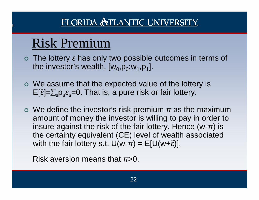
Risk Premium� The lottery ε has only two possible outcomes in terms of

the investor’s wealth, [w0,p0;w1,p1].

� We assume that the expected value of the lottery is E[ε]=∑spsεs=0. That is, a pure risk or fair lottery.

� We define the investor’s risk premium π as the maximum amount of money the investor is willing to pay in order to insure against the risk of the fair lottery. Hence (w-π) is the certainty equivalent (CE) level of wealth associated with the fair lottery s.t. U(w-π) = E[U(w+ε)].

Risk aversion means that π>0.

~

~

23

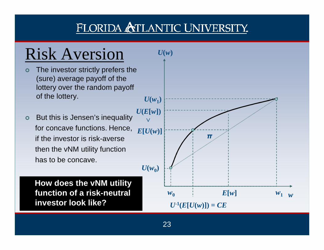
Risk Aversion� The investor strictly prefers the

(sure) average payoff of the lottery over the random payoff of the lottery.

� But this is Jensen’s inequalityfor concave functions. Hence,if the investor is risk-aversethen the vNM utility functionhas to be concave.

E[U(w)]

U(E[w])

w

U(w)

w0 w1

U(w0)

U(w1)

E[w]

U-1(E[U(w)]) = CE

>How does the vNM utility function of a risk-neutral investor look like?

π

24

� Note that U’’(w) < 0 if concave (risk aversion).

� Otherwise U’’(w) > 0 (risk preference).

� This is a property of the preference ordering.

Measures of risk-aversion:

A = -U’’(w)/U’(w) (Arrow-Pratt coefficient of absolute risk aversion)

R = -w·U’’(w)/U’(w) (Arrow-Pratt coefficient of relative risk aversion)

w

U(w)

w

U(w)Risk Aversion Risk Preference

25

Pratt’s (1964) Risk Premium:

We assume ε sufficiently small, so we can use a Taylor series approximation of U(w-π) = E[U(w+ε)] around ε = 0 and π = 0.

Expanding the left-hand side around π = 0 gives:

U(w-π) ≈ U(w) – πU’(w) + o(w)

Expanding the right-hand side around ε = 0 gives:

E[U(w+ε)] ≈ E[U(w) + εU’(w)+1/2ε2U’’(w)+o(w) ] = U(w)+1/2σ2U’’(w)

Where σ2= E[ε2] is the variance of the lottery. Equating both results and solving for the risk premium:

U(w) – πU’(w) = U(w)+1/2σ2U’’(w) → π = -1/2σ2U’’(w)/U’(w) = 1/2σ2A(w)

~ ~

~

~ ~ ~

~

26

Arrow’s (1971) Risk Premium:

We assume now that p0 = p1 = 1/2. How much it has to change the probability of winning to make the investor indifferent to the lottery?

π = p1 – p0 = p1 – (1 – p1) = 2p1 – 1 → p1 = 1/2 (1+π) and p1 = 1/2 (1-π)

These are risk-adjusted (neutral) probabilities. The expected utility of the lottery is:

U(w) = 1/2(1+π)U(w1)+1/2(1-π)U(w0). Taking a Taylor series approximation around ε = 0 gives:

U(w) =1/2(1+π)[U(w)+εU’(w)+1/2ε2U’’(w)+o(w)]+1/2(1-π)[U(w)-εU’(w)+1/2ε2U’’(w)+o(w)] = U(w)+επU’(w)+1/2ε2U’’(w)+o(w)

Rearranging terms and solving for π = -1/2εU’’(w)/U’(w) = 1/2εA(w)

Note that if we multiply π ε = 1/2ε2A(w) = Pratt’s measure.

~

~ ~

~ ~ ~ ~

~ ~

~ ~

27

-e-aw (Negative exponential)U’(w) =ae-aw

U’’(w) =-a2e-aw

A = -(-a2e-aw / ae-aw) = aR = wa

CARA Utility Functions

CRRA Utility Functions1/δ·wδ (Power)U’(w) =wδ-1

U’’(w) =(δ-1)wδ-2

A = - (δ-1)wδ-2 / wδ-1 = (1-δ)/wR = w (1-δ)/w = α

28

We note that constant relative risk aversion with decreasing absolute risk aversion seems to be more plausible than constant absolute risk aversion.Arrow on the other hand favored CARA + IRRA as evidence that money is a luxury good.

log w (Log) – Myopic utility function –U’(w) =1/wU’’(w) =-1/w2

A = -(-1/w2 / 1/w) = 1/wR = w / w = 1

If α < 1 then power preferences less risk averse than log preferences.

If α = 1 then power utility function collapses to log utility function.

If α > 1 then power preferences more risk averse than log preferences.

29

Name Function A R

Affine a+bw 0 0

Quadraticaw – 1/2bw2

w<a/bIncreasing Increasing

Exponential –e–aw a Increasing

Power w1–α /(1–α) Decreasing α

Bernoulli log w Decreasing 1

30

� All the utility functions in the previous table belong to the hyperbolic absolute risk aversion or HARA class (Alternatively affine risk tolerance functions or ART).

� Let absolute risk tolerance be defined as the reciprocal of absolute risk aversion T = A-1.

HARA Class of Utility Functions

U is HARA if T is an affine function T(w) = a + bw.

The slope b is sometimes called cautiousness.

31

General Form� Robert Merton show the general form of a HARA utility

function as:

DARA iff b > 0 (power & log),

CARA iff b = 0 (negative exponential), and

IARA iff b < 0 (quadratic), and

If one can prove a result for CARA and CRRA then one can prove a general result in the HARA class.

otherwise.

0,0 if

,1 if

,)()1(

,

),log(

)(/)1(1

/ >==

+−−

+=

−−

− ab

b

bwab

ae

wa

wUbb

aw

32

Choice under Uncertainty- Modern Approach -

33

� The strongest implication of the expected utility hypothesis comes from the form of the preference function: Is linear in probabilities.

� Assume the set of lotteries over the fixed wealth levels w1< w2< w3 represented by the set of all probability triples of the form: P=(p1, p2, p3), where pi = prob(wi), and Σpi = 1.

34

Marschak-Machina Triangle

� Since p2 = 1 – p1 - p3, we can represent the lotteries as points in the unit triangle.

� Note that northwest movements lead to stochastically dominating lotteries (they shift probability from w2 to w3 and from w1 to w2).

1

1

0 p1

p3

35

Risk Averse� The solid lines are indifference

curves.

� The dashed lines are iso-expected value lines, where going north-east implies mean preserving spread (pure increase in risk) over the average outcome w2 .

1

1

0 p1

p3

� For a risk-averse investor U(*) is concave and her indifference curves will be steeper than the iso-expected value lines.

36

Risk Lover

1

1

0 p1

p3

� For a risk-lover investor U(*) is convex and her indifference curves will be flatter than the iso-expected value lines.

37

vN-M Axioms(A1) Completeness

> For all P*, P either P* ffff P or P ffff P*.

(A2) Transitivity

> If P* ffff P and P ffff P** then P* ffff P**.

(A3) Continuity (Solvability)

> If P** ffff P* ffff P, then there exists some λ [0,1] s.t.

P* ~ λP** + (1-λ)P where the latter is a compound lottery.

~ ~

~ ~ ~

~ ~

38

P*

P**

αααα

1-αααα

P

P**1111−−−−αααα

αααα

(A4) Independence

> If P* ffff P then αααα P*+ (1- αααα) P** ffff αααα P+ (1- αααα) P**.

> Toss a fair coin with probability (1- αααα) of landing tails with prize equal to lottery P**, and be asked before the flip whether you would have rather P* or P in the event of a head. If it land tails the choice does not matter, otherwise you are in effect back to the choice P* or P and it would be rational to make the same choice than before (No regret).

Probability mixtures over a common outcome set

(A5) Stochastic Dominance> Let P1, P2 be two compound lotteries with parameters λ1, λ2 [0,1].

Then P1 ffff P2 iff λ1 > λ2 .

~ ~

39

The Allais Paradox

40

� Allais 1953, 1979.

A1: 1 chance of $ 1,000,000

versus

A2: 0.10 chance of $ 5,000,000

0.89 chance of $ 1,000,000

0.01 chance of $ 0

and

A3: 0.10 chance of $ 5,000,000

0.90 chance of $ 0

A4: 0.11 chance of $ 1,000,000

0.89 chance of $ 0

WHAT IS YOUR CHOICE?

Well it depends on your attitude towards risk…

1

1

0 p1

p3

A1

A2 A3

A4

41

� Paradox: Majority of subjects picked A1 in the first pair and A3 in the second pair.

� This implies that indifference curves are not parallel but fan out.

� This is a special case of a general pattern known as the common consequence effect.

1

1

0 p1

p3

A1

A2 A3

A4

42

� Intuitively the common consequence effect means that if the distribution of one of the lotteries involves very high outcomes, the investor prefers not to bear the extra risk in the unlucky event and consequently chooses the sure outcome.

� But if one distribution involves very low outcomes, the investor will be willing to bear the extra risk in the lucky event, and chooses the risky outcome.

The Common Consequence Effect

43

� The violation of the linear property in probabilities led researchers to generalize the expected utility model by deriving non-linear functionals for the preference function (Chew (1983), Fishburn (1983), Quiggin (1982) Machina (1982), Hey (1984), Segal (1984), Yaari (1987)).

� These are flexible specifications able to exhibit stochastic dominance, risk aversion, risk preference, and fanning out.

Non Expected Utility Models

44

Preference Reversal

45

� Slovic and Lichtenstein 1971.

P-bet: p chance of $ X

1-p chance of $ x

versus

$-bet: q chance of $ Y

1-q chance of $ y

where X and Y are respectively greater than x and y, p is greater than q, and Y is greater than X. The choice is between better probability of winning versus greater possible gain.

Any EU or N-EU model will imply that the chosen bet is the one with the higher CE or value.

Slovic an Lichtenstein and numerous authors after them found that subjects pick the P-bet although the $-bet has the largest value.

� Psychologists Interpretation

There is no common mechanism generating both choice and valuation (they are distinct processes).

Individuals exhibit response mode

effects or framing.

1) Context dependence (Duplex gambles, state dependent preferences).

2) Reference point (Markowitz, 1952, and Kahneman and Tversky, 1979).

46

� Kahneman and Tversky ‘s(1979) Prospect Theory.

The vNM utility should be a function of gains and losses in wealth with respect to some reference point (e.g., current wealth) instead of final wealth.

� Two problems with framing:

� Are experimental observations on framing effects for real?

� Is the reference point observable?

% change in Value

Utility

+100

-100

Reference point

47

Empirical Weighting Functions

48

� Economists Interpretation

Violation of transitivity axiom. Old issue in economics i.e., the existence of demand functions and general equilibrium are robust to intransitivity.

Expected regret model:

r(x,y) = -r(y,x)

Note that if r(x,y) = U(x)-U(y)

the model reduces to the EU model.

Graphically these preferences give indifference curves that cross forming an intransitive cycle.

Note though that near the origin they shouldn’t cross and transitivity holds. 1

1

0 p1

p3 p*

p

p**

49

50

51

Ellsberg’s Paradox

52

� Ellsberg 1961.

Which game would you choose?

Game 1 – Win $1,000 if you pick a red ball.

Game 2 – Win $1,000 if you pick a blue ball.

What about these?

Game 3 – Win $1,000 if you pick a red or yellow ball.

Game 4 – Win $1,000 if you pick a blue or yellow ball.

53

� The modal of subjects choose games 1 and 4. But yellow should not matter! So it seems that people prefer events with known probabilities.

� Ambiguity is uncertainty about probability created by missing information that is relevant and could be known.

� Does “weight of evidence”/ambiguity matters?� Longstanding debate:

� Savage: No.• Logic overrides discomfort of not knowing.

� Keynes, Knight, Ellsberg, experiments: Yes, agents are uncertainty averse.

� A New Paradigm (Gilboa-Schmeidler et al.)• Pessimism over sets of beliefs – Wald’s Maximin theory..• Non-additive beliefs.• Robust control theory.

54

Evidence: Neuroeconomics

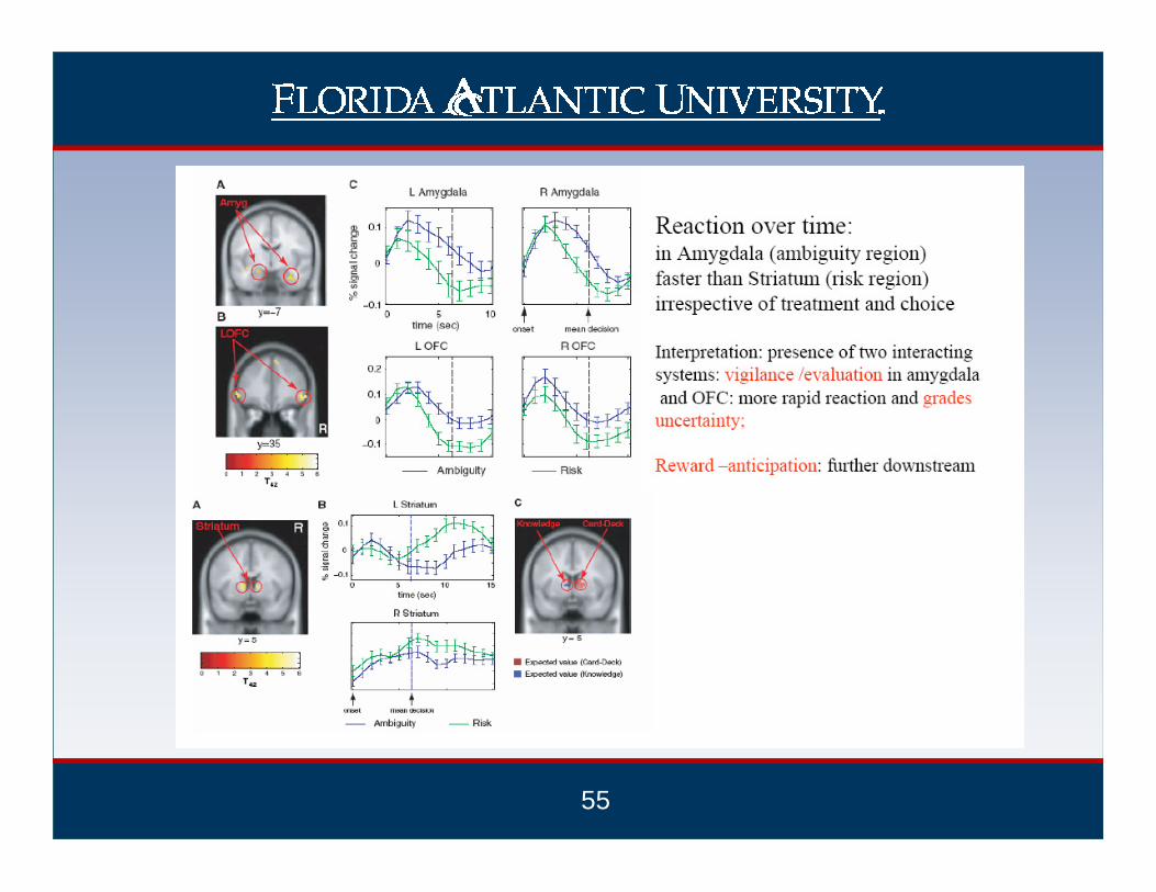
55

56

57

58

Conclusion

59

� The evidence and theories reported show the weaknesses of the standard paradigm.

� To what extent these new models will be incorporated into mainstream economic thought?

� The answer will depend on their capacity to address the issues better than the SEU model.