Ecological Modelling, 42 (1988) 199-215 199 Elsevier Science Publishers B.V., Amsterdam - Printed in The Netherlands

A M O D E L F O R THE R E L A T I O N S H I P BETWEEN LIGHT. I N T E N S I T Y A N D THE RATE OF P H O T O S Y N T H E S I S IN P H Y T O P L A N K T O N

P.H.C. EILERS 1 and J.C.H. PEETERS 2

Environmental Division, Delta Department, Rijkswaterstaat, P.O. Box 8039, 4330 EA Middelburg (The Netherlands)

(Accepted 20 January 1988)

ABSTRACT

Eilers, P.H.C. and Peeters, J.C.H., 1988. A model for the relationship between light intensity and the rate of photosynthesis in phytoplankton. Ecol. Modelling, 42: 199-215.

A dynamic model of the relationship between light intensity and the rate of photosynthe- sis in phytoplankton has been developed. The model describes the photosynthetic processes and those connected with photoinhibition and recovery from photoinhibition. In this paper, the steady-state properties of the model are studied and a production curve is derived from it. Simple expressions are derived for the maximum production rate Pm, the optimal and characteristic intensities I m and lk, and the initial slope of the curve. A new dimensionless parameter is introduced that measures the degree of photoinhibition. An iterative least-squares algorithm provides an easy method for fitting the parameters of the curve. It is proposed to present production curves in a dimensionless form (p /pm VS. I / Im) on logarithmic scales. This is especially useful in comparing different photosynthetic models. Comparison of the curve with those of Vollenweider and Platt et al. shows that they all behave similarly, except at high light intensities. The main advantage of this model compared to empirical curves is its foundation on physiological mechanisms. This makes it possible to derive effects of tempera- ture in a mechanistic way. A procedure is presented to integrate the phytoplankton produc- tion of a water column analytically.

INTRODUCTION

The influence of light intensity on the production and respiration of phytoplankton is the subject of extensive research. A large part of this

i Present address: Rijnmond Central Environmental Agency, 's-Gravenlandseweg 565, 3119 XT Schiedam, The Netherlands.

2 Present address: Section Biology, General Research, Tidal Waters Division, Rijkswa- terstaat, P.O. Box 8039, 4330 EA Middelburg, The Netherlands

0304-3800/88/$03.50 © 1988 Elsevier Science Publishers B.V.

200

research is aimed at a precise description of photosynthetic processes. Another part considers practical application to the description and analysis of ecological processes. This paper limits itself to the latter.

Measured production rates vs. intensities are often presented as points in a graph, together with a sketched (smooth) curve. Sometimes the datapoints are connected by straight line segments; see e.g. Fee (1973), for the compu- tation of production in a water column.

An improvement is the use of a parametric curve. If it fits well to the data and can be described by a few parameters, several advantages are obtained: the description is compact, the influence of random errors is reduced, characteristic parameters like the optimal intensity and maximal production rate can be calculated easily, and integration of production in a column of water may be performed analytically.

A number of proposals for production curves can be found in the literature, e.g. Smith (1936), Steele (1962), Vollenweider (1965) and P la t t e t al. (1980). They have been applied to experimental data more or less successfully; a recent systematic comparison was made by Iwakuma and Yasuno (1983). A common characteristic of most applications is that pro- duction curves are merely seen as mathematical equations that give a static picture of the dependence of the production rate on light intensity. A simple dynamic model for the essential processes of photoproduction and photoin- hibition can be far more useful to explain experimental results.

We present a model that is an improvement on one by Crill (1977). It also has strong connections to a proposal by Kok (1965). In Crill's model, hypothetical 'photosynthetic factories' (PSF) are used. The 'light' and 'dark' reactions are modeled by changes of the states of PSF's. Three states are possible and the dependences of the transition rates on light intensity and enzymatic activity determine the production curve that results from the model.

Crill proposed rather restricted and unrealistic transition probabilities, which forced him to introduce a hypothetical 'unit of light' (not a photon). Some simple modifications give a more realistic model that does not need such a construct.

From the model follows a system of three linear differential equations. The steady-state solution is a rational function with three parameters. Characteristics like optimal intensity and maximal production rate are easily derived. Together with a third derived parameter, which measures the peakedness of the production curve, a useful dimensionless formulation is obtained. This suggests the use of logarithmic scales. These scales are used for a comparison with other production curves.

The production curve that follows from the model was first published by Peeters and Eilers (1978). The same curve is used by Aiba (1982), who

201

presents it without derivation, by analogy with inhibition in enzyme kinetics. Megard et al. (1984) presented an essentially identical model.

We present an exact formula to calculate the integrated production in a water column, with constant extinction coefficient from the parameters of the production curve. The model gives valuable insights into the influence of temperature on the production curve.

For practical applications it is important that a curve can be fitted easily to experimental data. A special technique for rational functions (Wittmeyer, 1962) is simple to implement and gives good results.

METHODS

Photosynthesis measurements were conducted in Lund-type experimental reservoirs situated in a drinking-water basin (Van der Vlugt, 1976). Samples of the entire water column were incubated with 14C in an incubator by a procedure described by Birnbaum (1978). The amount of fixed carbon was measured by a technique described by Wessels and Birnbaum (1978).

MODEL DESCRIPTION

Structure of the model

Crill (1977) proposed a simple two-stage model. The first stage is light-de- pendent; it is represented by so-called photosynthetic factories (PSF) that can be imagined as a combination of Photosystems I and II (PSI and PSII). The second (dark) stage contains enzymatic reactions. We will only consider the first stage; there will be no second stage in the proposed model.

In Crill's model, a PSF processes one 'unit ' of light to give one 'uni t of photosynthetic product', in an interval At. The probability that a unit of light hits a PSF in At is denoted by p. The number of units per time is proportional to the intensity I, say f/ . If in At more than one hit occurs, the PSF gets inactivated and remains so until the end of the interval.

From these assumptions it follows that the production rate per PSF is proportional to the probability P of one and only one hit in At. From the binomial distribution it follows, with q = 1 - p :

( f I ) ! P - l!(f-I--- 1)! pqfl-1 (1)

If the number of PSF's is N, the total production rate will be proportional to:

NP = ( f N p / q ) I exp( f I ln(q)) (2)

202

If we introduce a = f N p / q and b = - f ln(q), it is easy to see that:

U P = aI e x p ( - b I ) (3)

This is identical to the production curve of Steele (1962). The behaviour of Crill's PSF can be represented by a graph as in Fig. la.

A unit of light hitting the PSF causes a transition from the resting state x 1 to the activated state x 2. The probabili ty of this transition is proportional to the intensity: this is indicated by a I along the arrow from x I to x 2. After an interval At, a unit of photosynthetic product is delivered and a transition to the resting state occurs. The curved arrow and the symbols (At) indicate this.

If the PSF is hit by another unit of light while it is in the activated state (x z), it goes into the inactivated state (x3). The probabil i ty of this transition is the same as for the transition from x a to x 2, as indicated by a I along the arrow from x 2 to x 3. While the PSF is in the inactivated state, more hits do not change the situation. After an interval At from the first hit, the PSF goes back into the resting state. This means that the symbols (At) along the arrow from x 3 to xa should not be read as At after the transition from x 2 to

X 3 •

The states and the transitions in Fig. l a give a useful basis for the representation of the three processes that are prominent in the behaviour of phytoplankton: no production (in the dark), photoproduct ion (in light) and photoinhibition (after some time, at higher intensities). However, the prob- abilities of the transitions, as proposed by Crill, do not seem to be very realistic. Some simple improvements will be presented now.

The transition from x2 to x 3 models photoinhibition. It is known (Kok, 1956; Jones and Kok, 1966) that photoinhibition develops slowly, compared to the nearly instantaneous changes in photoproduction, when light is switched on. This means that the probabili ty of inactivation has to be much smaller than aI . We introduce f lI for it.

It also seems improbable that both transitions back to x a occur after an exact interval At after the first hit, therefore we connect probabilities 3' and 6 to them, as in Fig. lb. The numerical value of 6 will be much smaller than that of y, because 7 corresponds to the photosynthetic dark reactions and 6 to repair from inhibition.

Photoproduct ion stops nearly directly after the light is switched off, while the recovery from photoinhibition can take a long time (see Myers and Burr, 1940; Kok, 1956; Belay and Fogg, 1978; Belay, 1981).

The probabilities in Fig. l b are per unit of time; see the derivation of differential equations which follows. We note that the modified PSF makes no use of the problematic processing interval At and the 'units ' of light and photosynthetic product.

203

Fig. 1. States and transition rates of a photosynthet ic factory (PSF) (a) in Crill 's model, (b) in the new model. The three states of a PSF are: x 1 resting state; x 2 activated state, x 3 inhibited.

We now derive the differential equations. Let the probabilities that a PSF is in one of the states x 1, x z or x 3 be represented by P1, Pz and/}3. The PSF can only be in one of these states, so:

PI + P2 + P3= I (4)

From the possible transitions follows:

P l ( t + d t ) = P l ( t ) - a I Pa(t) d t + y P2( t ) d t + 8 P3(t) dt

o r :

dPx - a l P I + y P 2 + S P 3 (5)

d t

In the same way we obtain:

dP2 d t - a l P 1 - ( f l I + Y)P2 (6)

d P 3 d t - f l i P 2 - ~P3 (7)

For given values of the parameters and I, this is a system of linear differential equations with constant - at a given value of I - coefficients,

204

that can be solved explicitly by classical means. In this paper we will restrict ourselves to the steady-state solution, when a constant intensity is main- tained long enough so that P1,P2 and P3 do not change anymore. Their steady-state values P1, P2 and P3 follow if we put the left-hand sides of the equations (5)-(7) to zero. The result is:

P1 = (/331-4- a 3 ) / F (8)

P z = a 3 I / F (9)

P, = a /312/F (10)

where

F = af l I 2 + (a + / 3 ) 8 1 + 73 (11)

The rate of photosynthetic production (p ) is proportional to the number of PSF's (N) and the number of transitions from x 2 to Xa:

p = kUfi2 = k a y 3 U I (12) af l I 2 + (a + f l ) 3 I + 3'3

Characteristics of the production curve

Equation (12) gives the relation between intensity and production rate in the steady state. It is expressed in the fundamental parameters k, N, a, /3, 3' and 6. Their values are generally unknown. For practical applications it is necessary to introduce a smaller set of parameters; their values have to be estimated from experimental data.

If we introduce:

/3 1 a - - - b c = ( 1 3 )

k y 3 N ' a k y N ' k a N

the result is:

I (14) P = aI 2 q_ bI + c

This is the equation for the production curve that was proposed by Peeters and Eilers (1978) and, independently, by Aiba (1982) and Megard et al. (1984).

Figure 2a shows the general shape of (14) and some characteristics of the curve. Equation (14) is easily interpreted algebraically: at low intensities, bI and aI 2 can be neglected and so the production rate increases approxi- mately linearly with intensity, while at high intensities aI 2 dominates and thus the production rate is inversely proportional to the intensity. Between

205

these extremes there is an optimum. As all the parameters in (14) are positive, p will be positive for every positive value of I. The characteristics in Fig. 2a are: s = tan(q~) initial slope; Pm maximal production rate; I m optimal intensity; and I k = Pm/S characteristic intensity. By differentiating (14), these characteristics can be expressed in the parameters a, b and c:

~ a 1 .

s = 1 / c ; Im = ; Pm b + 2 V r ~ '

The reverse equations are:

1 1 2 1 ;

a = slZm b = - - - , C = - - Pm SIm S

i k _ c ( 1 5 ) b +

(16)

The values of I m and Pm give the position and the height of the peak of the curve. A useful derived parameter that measures the sharpness of the peak is:

b I m w - - - - 2 (17)

t .

g

g o

o_

P .

I.

. 8 '

. 6 '

. 4 '

, 2 '

@ @

I I

I

I I

I n t e n s i t y

8

E

4

2

8 0

b

w-@

w--2

w-5 w-l@

Inten~ I ty

~ ~ C w-18 Wl5 Wl2

Intens I ty

m L

g

I n t e n s i t y

Fig. 2. Characteristics of the steady-state production curve. (a) Characteristic parameters. (b) Influence of the inhibition-parameter w when Pm and I m are fixed. (c) Idem, with I m and s fixed. (d) Influence of r , the probability of inhibition; a, y, 8 fixed.

206

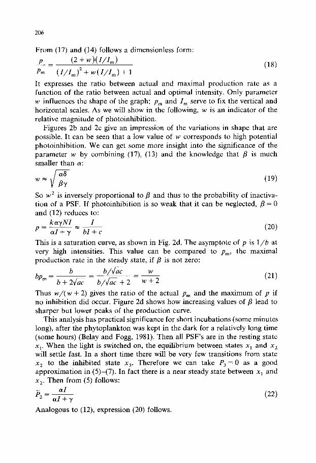
From (17) and (14) follows a dimensionless form:

p = (2 + w ) ( I / I m ) (18)

Pm ( U I m ) 2 + W ( I / I m ) + 1

It expresses the ratio between actual and maximal production rate as a function of the ratio between actual and optimal intensity. Only parameter w influences the shape of the graph; Pm and I m s e r v e to fix the vertical and horizontal scales. As we will show in the following, w is an indicator of the relative magnitude of photoinhibition.

Figures 2b and 2c give an impression of the variations in shape that are possible. It can be seen that a low value of w corresponds to high potential photoinhibition. We can get some more insight into the significance of the parameter w by combining (17), (13) and the knowledge that fl is much smaller than a:

~ / a 6 (19) w = 13~,

So w 2 is inversely proportional to 13 and thus to the probability of inactiva- tion of a PSF. If photoinhibition is so weak that it can be neglected, 13 = 0 and (12) reduces to:

k a g N I I (20) P - a I + y b I + c

This is a saturation curve, as shown in Fig. 2d. The asymptote of p is 1 / b at very high intensities. This value can be compared to Pm, the maximal production rate in the steady state, if 13 is not zero:

bp m _ b _ b/vra7 _ w (21) b + 27'a7 b / v / ~ + 2 w + 2

Thus w / ( w + 2) gives the ratio of the actual Pm and the maximum of p if no inhibition did occur. Figure 2d shows how increasing values of 13 lead to sharper but lower peaks of the production curve.

This analysis has practical significance for short incubations (some minutes long), after the phytoplankton was kept in the dark for a relatively long time (some hours) (Belay and Fogg, 1981). Then all PSF's are in the resting state x a. When the fight is switched on, the equilibrium between states x I and x 2 will settle fast. In a short time there will be very few transitions from state x 2 to the inhibited state x 3. Therefore we can take P3 = 0 as a good approximation in (5)-(7). In fact there is a near steady state between x I and x z. Then from (5) follows:

a I (22) P2-- ~ i + y

Analogous to (12), expression (20) follows.

207

Thus, short incubations lead to a saturation curve instead of an inhibition curve. Photoinhibition needs time to develop and become measurable. This has been reported by Myers and Burr (1940), Kok (1956), Harris and Piccinin (1977), Harris (1978), Marra (1978), Belay (1981) and Whitelam and Codd (1983).

The relatively slow development of - and recovery from - photoinhibi- tion is probably the basis of hysteresis phenomena that are reported in the literature (Cosby et al., 1984; Denman and Marra, 1986; Neale and Richer- son, 1987).

Logarithmic scales and compar&on to other production curves

A further simplification of the shapes of production curves is obtained when logarithmic scales are used for graphs. If we put:

q = l n ( p / p m ) , u = In (U/m) (23)

the result is:

q = l n ( w + 2 ) + l n e x p ( u ) + w + e x p ( - u )

Figure 3a shows graphs of production curves for some values of w with identical initial slopes. The optimal intensity is 1 (arbitrary units). Sharper peaks correspond to smaller values of w. It is seen that the graphs are symmetric with respect to Im. That follows easily from (24) as u and - u give the same value for q.

At both very low and very high intensities, the graphs approach straight lines. At very low intensities exp ( -u ) dominates e x p ( u ) + w , thus (24) simplifies to:

(11 q ~ l n ( w + 2 ) + l n e x p ( - u ) = u + l n ( w + 2 ) (25)

By analogous reasoning we find at very high intensities:

q = - u + l n ( w + 2 ) (26)

Every curve of equation (14) will, on logarithmic scales, be shaped like the curves in Fig. 3a; different values of I m will give a horizontal displacement and different values of Pm will give a vertical displacement.

Logarithmic scales are useful for a comparison with different production curves from the literature. Figure 3b illustrates the equation from Vol- lenweider (1965):

a / ( 1 )" (27) P - ~1 + b2I 2 (1 + c2I 2

208

L

8

o

| -

- | -

- 2 -

- 3 -

- 4 -

- 5 -3

1-

NEN MODEL

a

I

I I I I I ! - 2 - I B 1 2 3

LOG( I n t e n = I t y )

V O L L E N N E I D E R (N-2)

c

B-

_:a_

- 4 -

--S I I I I I I - 3 - 2 - t B I 2 3

L O G ( l n t a n = I t y )

L

8

:J

o

o ..I

V O L L E N N E I D E R (N- l )

b 0-

- 2 - /

- 4 -

--S I I I I I - 3 - 2 - 1 B 1 2

L O G ( Z n t e n = l t y )

PLRTT,GRLLEGOS L HRRRZSON

l - d

8 -

- 1 - ~

- 2 -

- 4 -

- 5 I - 3 - 2 - 1 9 I 2 3

L O G ( I n t e n = l t y )

Fig. 3. Comparison of four types of production curves on logarithmic scales: (a) new model (equation 18); (b) Vollenweider's model (equation 27), n =1; (c) idem, n = 2; (d) model of Platt, Gallegos and Harrison (equation 28).

for n = 1. The initial slope is chosen the same for every curve, as is I m. The differences with Fig. 3a are very small. The curves are symmetric and the asymptotes are straight lines. The peaks are somewhat flatter.

Other curves show greater differences. If we choose n = 2 in (27), Fig. 3c results. To the left of the peak the shape is practically the same as in the Figs. 3a and 3b. At high intensities, however, the inhibition increases more rapidly. From (27) it follows that p is inversely proportional to 12. Iwakuma and Yasuno (1983) proposed a four-parameter generalization of Vol- lenweider's curve that can give any slope - n / m for the right asymptote.

An even faster decrease of p with 1 is shown by the curve of Platt et al. (1980):

p = a ( e - b l - - e -C') (28)

209

It is graphed in Fig. 3d. At high intensities, p decreases exponentially with I and there is no asymptote.

The curve with the sharpest peak in Figure 3d is the graph of Steele's curve (Steele, 1962). It is the limit of (28) if b and c are nearly equal: then

p = a ( c - b ) I e -bl (29)

From the comparison above it follows that the equations only differ essentially at higher intensities, in the way in which they model photoinhibi- tion. This means that a clear experimental discrimination can only be made by precise measurements at intensities 5 or 10 times Im.

F I T T I N G T H E C U R V E TO E X P E R I M E N T A L D A T A

For practical applications of the model in (14), the parameters a, b and c are to be estimated in such a way that the curve conforms as well as possible to pairs of measurements (Ii, p,, i = 1, . . . , n). A simple approach is to fit 1/p:

1 - - = a I 2 + b I + c (30) P

This method is used by Megard et al. (1984) but is not to be recommended. Small values of p give high values of 1/p that have a large influence on the parameter estimates. But small values of p have a large relative error and so 1/p has a large relative and absolute error. Thus the most influential data points are the most unreliable ones. This gives unnecessarily large errors in the estimated parameters (Roberts, 1977).

There exist numerous general minimization techniques that can be used to solve this curve-fitting problem. Good computer programs, however, are not generally available. Therefore it is attractive to use a simpler technique that exploits the special structure of the problem.

An efficient and robust method for fitting rational functions like (14) was proposed by Wittmeyer (1962); the idea is to transform a nonlinear regres- sion problem in a sequence of weighted linear regression problems. Let:

= 1, ( 3 1 ) aI,2 + +

be the estimated production rate at intensity Is, for estimated parameter values d, b and g. According to the principle of least squares, we seek parameter values that minimize:

n

s = (p , (32) i = 1

210

Substitute (31) in (32):

( ,/ t S = i=]Y: Pi-- ali2 + ~ii + ~

This can be written as:

(33)

Minimize:

S= L l~i2(pi(ali2+bli+c)-l i) 2 i = 1

(34)

5-

4-

3-

2-

l-

O ol

: m g ( C ) / m g ( C h l ) / h )

4-

3-

2-

l -

g IB t~e 2ee 3ee 4ae

(H/m2]

5 - ( m g ( C ) / m g ( C h l ) / h ]

5-

4-

3-

2-

! -

O~

tea z~e 3~e 4ee (Him2')

5 -1 [mg(C) /mg(Ch l ) / h )

4-

3-

2-

1-

8 . t~e a~e 3~e 4.e

[N/m2)

[ m g ( C ) / m g ( C h l ) / h )

t~e 2ee 380 4~e (N/m2)

5 - [ m g ( C ) / m g ( C h l ) / h ]

4-

2-

L-

5°

4,

3-

2-

1-

8

~mg(C) Img(Ch l ) l h3

f 8 e l~e 2ee 3~e 4~e e lee 2ee 3ee 4~e

(N/m2 ] (N#m2 ]

Fig. 4. Examples of measured data and fitted curves. These examples were selected as representative for different situations (weak/strong photoinhibition; good/moderate fit of curve).

211

where

1 (35) wi = aL 2 + [,Ii +

Minimization of (34) specifies a weighted linear regression problem that can easily be solved if the weights W~ are known. These, however, are to be computed from the parameters that are to be estimated! To break this vicious circle, Wittmeyer proposes to start with rough estimates for a, /~ and

in (35). From the solution of (34), improved estimates follow that are used in the next iteration, etc.

In general, Wittmeyer 's method works well. After four or five iterations the values of the parameters do not change more than 1%o. To start the iterations, very crude estimates (fi = 0, b = 0 and ~ = 1) suffice. In a few cases slow convergence or oscillations were observed. Figure 4 gives results for some typical data sets.

APPLICATIONS

Integrated production in a column of water

An important application of production curves is the computat ion of integrated production at steady state in a column of water. If the concentra- tion of phytoplankton and the extinction coefficient (c) are constant be- tween depths z 1 and z2, the integrated rate of production per unit of biomass will be:

= fZ2p ( l ( z ) ) dz (36) P Z 1

If we put:

I o = I ( 0 ) , 11 = I ( z l ) , 12=I ( z2 ) (37)

it follows that

I ( z ) = 11 e x p ( - , ( z - Z1) ) = I 0 e x p ( - , z ) (38)

The integral to solve is:

rz2 I o e x p ( - c z ) dz

P = J-zl aI 2 e x p ( - z c z ) + bI o e x p ( - ~ z ) + c (39)

From (38) follows:

d I = - I 0 e x p ( - c z ) dz (40)

212

and also

p = _ _1 f12 d I E ,]111 a I 2 + b I + c

The analytic solution is known:

dz _ 2 arctan ax2 + bx + c v / - D

- 2

a x + b

= 1 l n ( 2 a x + b - v r ~ )

V ~ 2ax + b + ~/-D

where

D = b 2 - 4ac

If we put:

B 1 = 2aI 1 + b, B 2 = 2aI 2 + b

the final result for P is:

_ 2 arctan( B1 - P e~/-Z~ , - - ~ - ) arctan( _ ~ D )

1) p = -

E B 2 B 1

1 ( (B1 - fD)(B2 + v ~ ) P = c v ~ In (B1 + v ~ ) ( B 2 - - ~/~)

(41)

if D < 0

if D = 0 (42)

if D > O

(43)

(44)

if D < 0

if D = 0 (45)

if D > 0

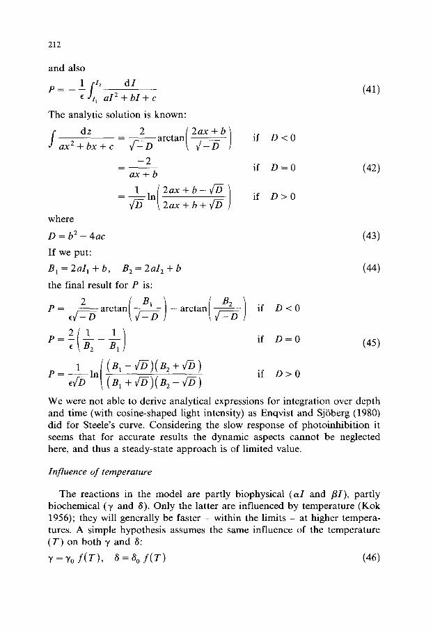
We were not able to derive analytical expressions for integration over depth and time (with cosine-shaped light intensity) as Enqvist and SjSberg (1980) did for Steele's curve. Considering the slow response of photoinhibition it seems that for accurate results the dynamic aspects cannot be neglected here, and thus a steady-state approach is of limited value.

Influence of temperature

The reactions in the model are partly biophysical ( a I and i l l ) , partly biochemical (V and 8). Only the latter are influenced by temperature (Kok 1956); they will generally be faster - within the limits - at higher tempera- tures. A simple hypothesis assumes the same influence of the temperature (T) on both 3' and 3:

3 ' = Y o f ( T ) , 8 = 3 o f ( T ) (46)

213

1 - -

-2--

-] _

/ / /

-5 I

- ] -2

f ~ / \ p t - . . . \

.// .. \ \ i " ", ", \

~ \ \ N \ \ T3

\

, T2

T 1< T 2 <T 3 " .

I I I I I -1 0 1 2 3

LOG ( intensi ty)

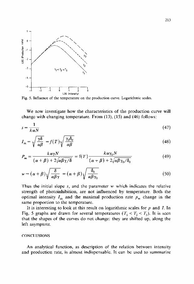
Fig. 5. Influence of the temperature on the production curve. Logarithmic scales.

We now investigate how the characteristics of the production curve will change with changing temperature. From (13), (15) and (46) follows:

1 s - kerN (47)

~/-£Y+ 7 y°8° (48) im= y3 = f ( T ) aft

Pm = k a v N _ _ = f (T) kay°N (49) ( a + fl) + 2 ~ / 3 (a + fl) + 2~/aflVo/3o

7- 7 8 - (~ + B) 80 (5o) w = (~ + B) ~Bv ~Bv0

Thus the initial slope s, and the parameter w which indicates the relative strength of photoinhibition, are not influenced by temperature. Both the optimal intensity I m and the maximal production rate Pm change in the same proportion to the temperature.

It is interesting to look at this result on logarithmic scales for p and I. In Fig. 5 graphs are drawn for several temperatures (T 1 < T 2 < T3). It is seen that the shapes of the curves do not change: they are shifted up, along the left asymptote.

CONCLUSIONS

An analytical function, as description of the relation between intensity and production rate, is almost indispensable. It can be used to summarize

214

experimental data, to reduce the effects of random errors in the measure- ments, and to compute integrated production in a column of water.

The new curve we propose in this paper does not show many differences to the curves proposed by Vollenweider and Platt c.s. Only at very high intensities a clear discrimination is possible. Often measurements will not cover a large enough range of intensities to make the distinction clear.

However, an important advantage of our results is that they are based on a simple model that gives a dynamic description of photosynthesis and photoinhibition. By extending Crill's model, a plausible mechanism resulted that gives explicit equations for both processes.

Even if one only investigates the steady state, the advantages of a model are clear. This was illustrated by the analysis of the effect of temperature changes on the characteristics of the production curve, and by the discussion of the difference between long and short incubations.

Wittmeyer's algorithm provides a rapid and practical method for fitting the three parameters of the curve to measured data of intensity and production rate.

Presentation of production curves on logarithmic scales has certain ad- vantages, because changes in two of the three parameters of the production curve correspond only to a shift in the curve, without a change in shape.

ACKNOWLEDGEMENTS

The measurements which have been presented were processed by Eli Birnbaum and Peter Havermans. Wim Bil made most programs. We greatly appreciated their help. We thank O. Klepper and L.P.M.J. Wetsteyn for reading the manuscript.

REFERENCES

Aiba, S., 1982. Growth kinetics of photosynthetic micro-organisms. In: A. Fiechter (Editor), Microbial Reactions. Adv. Biochem. Eng., 23: 85-156.

Belay, A., 1981. An experimental investigation of inhibition of phytoplankton photosynthesis at lake surfaces. New Phytol., 89: 61-74.

Belay, A. and Fogg, G.E., 1978. Photoinhibition of photosynthesis in Asterionella formosa (Bacillariophyceae). J. Phycol., 14: 341-347.

Birnbaum, E.L., 1978. Estimating in situ algal production rates with the help of light measurements and experimentally measured production rates. Hydrobiol. Bull., 12: 127-133.

Cosby, B.J., Hornberger, G.M. and Kelly, M.G., 1984. Identification of photosynthesis-light models for aquatic systems. II. Application to a macrophyte dominated stream. Ecol. Modelling, 23: 25-51.

Crill, P.A., 1977. The photosynthesis-light curve: a simple analog model. J. Theor. Biol., 6: 503-516.

215

Denman, K.L. and Marra, J., 1986. Modelling the time dependent photoadaptation of phytoplankton to fluctuating light. In: J.C.J. Nihoul (Editor), Marine Interfaces Ecohydrodynamics. Elsevier, Amsterdam, pp. 341-349.

Enqvist, A. and Sj~berg, S., 1980. An analytical integration method of computing diurnal primary production from Steele's light response curve. Ecol. Modelling, 8 :219 232.

Fee, E.J., 1973. Modelling primary production in water bodies: a numerical approach that allows vertical inhomogeneities. J. Fish. Res. Board Can., 30: 1469-1473.

Harris, G.P., 1978. Photosynthesis, productivity and growth. The physiological ecology of phytoplankton. Ergebn. Limnol., 10: 1-171.

Harris, G.P. and Piccinin, B.B., 1977. Photosynthesis by natural phytoplankton populations. Arch. Hydrobiol., 80: 405-457.

Iwakuma, T. and Yasuno, M., 1983. A comparison of several mathematical equations describing photosynthesis-light curve for natural phytoplankton populations. Arch. Hy- drobiol., 97: 208-226.

Jones, L.W. and Kok, B., 1966. Photoinhibition of chloroplast reactions. I. Kinetics and action spectra. Plant Physiol., 41: 1037-1043.

Kok, B., 1956. On the inhibition of photosynthesis by intense light. Biochem. Biophys. Acta, 21: 234-244.

Marra, J., 1978. Phytoplankton photosynthetic response to vertical movement in a mixed layer. Mar. Biol., 46: 203-208.

Megard, R.O., Tonkyn, D.W. and Senft, W.H., 1984. Kinetics of oxygenic photosynthesis in planktonic algae. J. Plankton Res., 6: 325-337.

Myers, J. and Burr, G.O., 1940. Studies on photosynthesis. Some effects of light of high intensity on Chlorella. J. Gen. Physiol., 24: 45-67.

Neale, P.J. and Richerson, P.J., 1987. Photoinhibition and diurnal variation of phytoplankton photosynthesis - I. Development of a photosynthesis irradiance model from studies of in situ responses. J. Plankton Res., 9: 167-193.

Peeters, J.C.H. and Eilers, P., 1978. The relationship between light intensity and photosynthe- sis. A simple mathematical model. Hydrobiol. Bull., 12: 134-136.

Platt, T., Gallegos, C.L. and Harrison, W.G., 1980. Photoinhibition and photosynthesis in natural assemblages of marine phytoplankton. J. Mar. Res., 38:687 701.

Roberts, D.V., 1977. Enzyme Kinetics. Cambridge University Press, Cambridge, 326 pp. Smith, E.L., 1936. Photosynthesis in relation to light and carbon dioxide. Proc. Nat. Acad.

Sci., 22: 504-511. Smith, R.A., 1980. The theoretical basis for estimating phytoplankton production and specific

growth rate from chlorophyll, light and temperature data. Ecol. Modelling, 10: 243-264. Steele, J.H., 1962. Environmental control of photosynthesis in the sea. Limnol. Oceanogr., 7:

137-150. Van der Vlugt, J.C., 1976. Comparative limnological research in the 'Grote Rug' and model

reservoirs. Hydrobiol. Bull., 10: 136-144. Vollenweider, R.A., 1965. Calculation models of photosynthesis-depth curves and some

implications regarding daily rate estimates in primary production measurements. Mem. Ist. Ital. Idrobiol., 18 (Suppl.): 425-457.

Wessels, Ch. and Birnbaum, E.L., 1979. An improved apparatus for use with the 14C acid-bubbling method for measuring primary production. Limnol. Oceanogr., 14: 187-188.

Whitelam, G.C. and Codd, G.A., 1983. Photoinhibition of photosynthesis in the cyanobac- terium Microcystis aeroginosa. Planta, 157: 561-566.

Wittmeyer, L., 1962. Rational approximations of empirical functions. BIT, 2: 53-60.